2 Upper bound on $\pi _2(x)$

To calculate B, we require an upper bound on the twin prime counting function $\pi _2(x) := \#\{p \text { prime}: p+2 \text { also prime}\}$ . We derive this bound using Selberg’s sieve by sieving on the set of odd numbers n such that $n-2$ is prime. If n is removed by the sieve (that is, n is not prime), then $(n-2,n)$ cannot form a twin prime pair.

2.1 Preliminaries

For an introduction to Selberg’s sieve, see [Reference Halberstam and Richert5]. We begin by defining some preliminary notation. Our set of twin prime candidates is given by

$$ \begin{align*} \mathcal{A} = \{n \leq x+2: n\text{ odd with }n-2 \text{ prime}\} \end{align*} $$

and our set of sieving primes by

$$ \begin{align*} \mathcal{P}=\{p>2:p\text{ prime}\}. \end{align*} $$

We will be sieving using odd primes less than or equal to z, and so we set

$$ \begin{align*} P_z= \prod_{\substack{p \in\mathcal{P}\\ p\leq z}}{p}. \end{align*} $$

Next, $\mathcal {A}_d$ is the set of twin prime candidates that are divisible by a specific prime d, and

$$ \begin{align*} A_d= |\{n \leq x+2:d \mid n \text{ and } n-2 \text{ is prime}\}| = \pi(x;d,-2). \end{align*} $$

By the prime number theorem in arithmetic progressions, we can estimate $\pi (x;d,-2)$ by ${\text {li}(x)}/{\varphi (d)}$ , and so we define the error in our estimation to be

$$ \begin{align*} E(x;d):= \pi(x;d,-2) - \frac{\text{li}(x)}{\varphi(d)}, \end{align*} $$

where

$$ \begin{align*} \text{li}(x) := \int_2^x\,\frac{dt}{\log{t}}. \end{align*} $$

As we take li to be truncated at 2, it will be useful to define the offset as

$$ \begin{align*} \text{li}_2:=\int_0^2\,\frac{dt}{\log{t}}. \end{align*} $$

The twin prime constant is

$$ \begin{align*} \pi_2 := \prod_{p>2}\frac{p(p-2)}{(p-1)^2}. \end{align*} $$

Following Klyve [Reference Klyve7, page 128], we take

$$ \begin{align*} V(z) = \sum_{\substack{d \leq z \\ d|P_z}}{\frac{1}{\prod_{p|d}{(p-2)}}}. \end{align*} $$

And finally, we set

$$ \begin{align*} [d_1,d_2]:=\text{lcm}(d_1,d_2). \end{align*} $$

Theorem 2.1 [Reference Klyve7, Theorem 5.7].

For $0<z<x$ ,

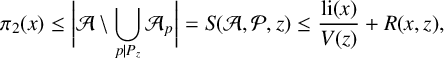$$ \begin{align*} \pi_2(x) \leq \bigg|\mathcal{A} \setminus \bigcup_{p|P_z} \mathcal{A}_p\bigg| = S(\mathcal{A},\mathcal{P}, z) \leq \frac{\mathrm{li}(x)}{V(z)}+ R(x,z), \end{align*} $$

where we have defined

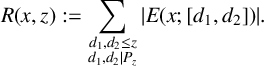$$ \begin{align*} R(x,z):= \sum_{\substack{d_1, d_2 \leq z \\ d_1,d_2 | P_z}}{|E(x;[d_1,d_2])|}. \end{align*} $$

2.2 Bounding $V^{-1}(z)$

We need to provide an upper bound on $V^{-1}(z)$ for all z. As z increases, computing $V(z)$ directly becomes infeasible, requiring a trade-off between accuracy and efficiency. To address this, we will consider three separate intervals (separated by values $L_1$ and $L_2$ ), with different bounds on $V(z)$ for each interval. For our calculations, we set $L_1 = 10^8$ and $L_2 = 10^{10}$ .

For the first interval ( $z < L_1$ ), we compute $V(z)$ exactly. For the second interval ( $L_1 < z \leq L_2$ ), we compute $V(z')$ exactly, where $z' \in \{L_1<z\leq L_2: z=k\cdot 10^4, k \in \mathbb {N}\}$ (that is, every $10^4$ th number). For the values of z such that $10^4 \nmid z$ , we can round z down to the nearest $z'$ to give an upper bound on $V^{-1}(z)$ . For the third interval, we will use the approximation of $V(z)$ derived in [Reference Klyve7, Section 5.5.2], namely

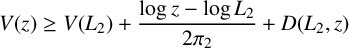$$ \begin{align*} V(z) \geq V(L_2) + \frac{\log{z}-\log{L_2}}{2\pi_2} + D(L_2,z) \end{align*} $$

where

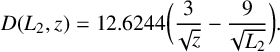$$ \begin{align*} D(L_2,z) = 12.6244\bigg(\frac{3}{\sqrt{z}} - \frac{9}{\sqrt{L_2}}\bigg). \end{align*} $$

The following lemma summarises these arrangements.

Lemma 2.2. For any z, we have

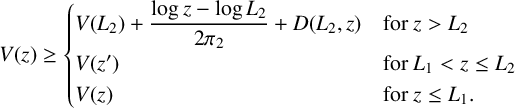$$ \begin{align*}V(z) \geq \begin{cases} V(L_2) + \dfrac{\log{z}-\log{L_2}}{2\pi_2} + D(L_2,z) & \mbox{for }z> L_2\\ V(z') & \mbox{for }L_1 <z \leq L_2 \\ V(z) & \mbox{for } z\leq L_1. \end{cases}\end{align*} $$

2.3 Bounding $R(x,z)$

Next, we need an upper bound on $R(x,z)$ for all x and z. We will start by proving an inequality that will allow us to bound one of the terms of $R(x,z)$ . This inequality holds for any fixed prime p, but becomes less useful as the size of p increases relative to the size of z. We have excluded some slight optimisations on the order of $z^{1/2}$ for the sake of readability, and the range of permissible values of z can be lowered at a similar cost. For our case, we will be setting $p=2$ .

Proposition 2.3. Let p be a prime and $z \geq 2\,768\,896$ . Then

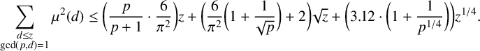$$ \begin{align*} \sum_{\substack{d \leq z \\ \mathrm{gcd}(p,d)=1}}{\mu^2(d)} \leq \bigg(\frac{p}{p+1}\cdot \frac{6}{\pi^2}\bigg)z + \bigg( \frac{6}{\pi^2}\bigg(1+\frac{1}{\sqrt{p}}\bigg)+2\bigg)\sqrt{z} + \bigg(3.12 \cdot\bigg(1+\frac{1}{p^{1/4}}\bigg)\bigg)z^{1/4}. \end{align*} $$

Proof. To start, note that we can write

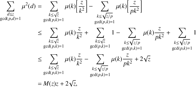$$ \begin{align*} \sum_{\substack{d \leq z \\ \mathrm{gcd}(p,d)=1}}{\mu^2(d)} &= \sum_{\substack{k \leq \sqrt{z} \\ \mathrm{gcd}(p,k)=1}}\mu(k)\bigg[\frac{z}{k^2}\bigg] - \sum_{\substack{k \leq \sqrt{{z}/{p}} \\ \mathrm{gcd}(p,k)=1}}\mu(k)\bigg[\frac{z}{pk^2}\bigg] \\ &\leq \sum_{\substack{k \leq \sqrt{z} \\ \mathrm{gcd}(p,k)=1}}\mu(k)\frac{z}{k^2} + \sum_{\substack{k \leq \sqrt{z} \\ \mathrm{gcd}(p,k)=1}}1 - \sum_{\substack{k \leq \sqrt{{z}/{p}} \\ \mathrm{gcd}(p,k)=1}}\mu(k)\frac{z}{pk^2} +\sum_{\substack{k \leq \sqrt{{z}/{p}} \\ \mathrm{gcd}(p,k)=1}}1\\ &\leq \sum_{\substack{k \leq \sqrt{z} \\ \mathrm{gcd}(p,k)=1}}\mu(k)\frac{z}{k^2} - \sum_{\substack{k \leq \sqrt{{z}/{p}} \\ \mathrm{gcd}(p,k)=1}}\mu(k)\frac{z}{pk^2} + 2 \sqrt{z}\\ &= M(z)z + 2 \sqrt{z}, \end{align*} $$

where we have taken

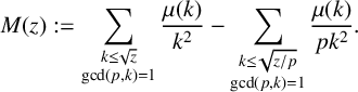$$ \begin{align*} M(z) :=\sum_{\substack{k \leq \sqrt{z} \\ \mathrm{gcd}(p,k)=1}}\frac{\mu(k)}{k^2} - \sum_{\substack{k \leq \sqrt{{z}/{p}} \\ \mathrm{gcd}(p,k)=1}}\frac{\mu(k)}{pk^2}. \end{align*} $$

Also, for $p'$ any prime number,

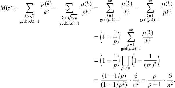$$ \begin{align*} M(z) + \sum_{\substack{k> \sqrt{z} \\ \mathrm{gcd}(p,k)=1}}\frac{\mu(k)}{k^2} - \sum_{\substack{k > \sqrt{{z}/{p}} \\ \mathrm{gcd}(p,k)=1}}\frac{\mu(k)}{pk^2} &= \sum_{\substack{k=1 \\ \mathrm{gcd}(p,k)=1}}^{\infty}\frac{\mu(k)}{k^2} - \sum_{\substack{k =1 \\ \mathrm{gcd}(p,k)=1}}^{\infty}\frac{\mu(k)}{pk^2} \\ &=\bigg(1-\frac{1}{p}\bigg)\sum_{\substack{k=1 \\ \mathrm{gcd}(p,k)=1}}^{\infty}\frac{\mu(k)}{k^2} \\ &=\bigg(1-\frac{1}{p}\bigg)\prod_{p' \neq p}\bigg(1-\frac{1}{(p')^2}\bigg)\\ &=\frac{(1-{1}/{p})}{(1-{1}/{p^2})} \cdot \frac{6}{\pi^2} =\frac{p}{p+1} \cdot \frac{6}{\pi^2}. \end{align*} $$

Now we can bound the difference

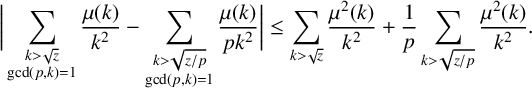$$ \begin{align*} \bigg|\sum_{\substack{k> \sqrt{z} \\ \mathrm{gcd}(p,k)=1}}\frac{\mu(k)}{k^2} - \sum_{\substack{k > \sqrt{{z}/{p}} \\ \mathrm{gcd}(p,k)=1}}\frac{\mu(k)}{pk^2} \bigg| \leq \sum_{k > \sqrt{z}}\frac{\mu^2(k)}{k^2} + \frac{1}{p}\sum_{k > \sqrt{{z}/{p}} }\frac{\mu^2(k)}{k^2}. \end{align*} $$

We now apply explicit bounds on the square-free summation function provided in [Reference Cohen, Dress, Daboussi, Deshouillers and Liardet2], in conjunction with partial summation, to note that

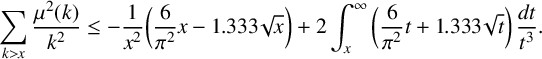$$ \begin{align*} \sum_{k> x}\frac{\mu^2(k)}{k^2} \leq -\frac{1}{x^2}\bigg(\frac{6}{\pi^2}x - 1.333\sqrt{x}\bigg) + 2\int_{x}^{\infty} \bigg(\frac{6}{\pi^2}t + 1.333\sqrt{t}\bigg) \,\frac{dt}{t^3}. \end{align*} $$

Applying this substitution, and simplifying terms, we conclude that

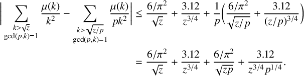$$ \begin{align*} \bigg|\sum_{\substack{k> \sqrt{z} \\ \mathrm{gcd}(p,k)=1}}\frac{\mu(k)}{k^2}- \sum_{\substack{k > \sqrt{{z}/{p}} \\ \mathrm{gcd}(p,k)=1}}\frac{\mu(k)}{pk^2} \bigg| &\leq \frac{{6}/{\pi^2}}{\sqrt{z}} + \frac{3.12}{z^{3/4}} + \frac{1}{p}\bigg(\frac{{6}/{\pi^2}}{\sqrt{{z}/{p}}} + \frac{3.12}{({z}/{p})^{3/4}} \bigg)\\ &= \frac{{6}/{\pi^2}}{\sqrt{z}} + \frac{3.12}{z^{3/4}} + \frac{{6}/{\pi^2}}{\sqrt{zp}} + \frac{3.12}{z^{3/4}p^{1/4}}. \end{align*} $$

Combining this result with the first inequality proves the lemma.

In a similar manner to $V(z)$ , the sum $\sum _{ {d \leq z,\, \mathrm {gcd}(2,d)=1}}{\mu ^2(d)}$ becomes infeasible to compute for large values of z. We employ a similar technique of approximating $\sum _{{d \leq z, \,\mathrm {gcd}(2,d)=1}}{\mu ^2(d)}$ for z larger than a specific cut-off value $L_3$ (using Proposition 2.3), and calculating it exactly for the remaining values. We take $L_3=10^7$ for our calculations.

Lemma 2.4. For any z,

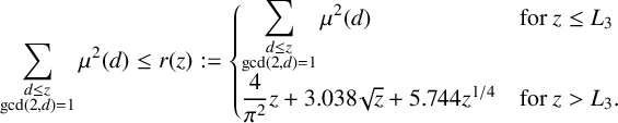$$ \begin{align*} &\sum_{\substack{d \leq z \\ \mathrm{gcd}(2,d)=1}}{\mu^2(d)} \leq r(z):= \begin{cases} \displaystyle\sum_{\substack{d \leq z \\ \mathrm{gcd}(2,d)=1}}{\mu^2(d)} & \mbox{for } z \leq L_3 \\ \dfrac{4}{\pi^2}z + 3.038\sqrt{z} + 5.744z^{1/4} & \mbox{for } z>L_3. \end{cases} \end{align*} $$

Theorem 2.5. Assuming GRH, for $x \geq 4\cdot 10^{18}$ and $z<x^{{1}/{4}}$ ,

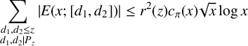$$ \begin{align*} \sum_{\substack{d_1, d_2 \leq z \\ d_1,d_2 | P_z}}{|E(x;[d_1,d_2])|} \leq r^2(z)c_\pi(x)\sqrt{x}\log{x} \end{align*} $$

where

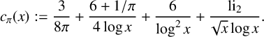$$ \begin{align*} &c_\pi(x) := \frac{3}{8\pi} + \frac{6+1/\pi}{4\log{x}} + \frac{6}{\log^2{x}} + \frac{\mathrm{li}_2}{\sqrt{x}\log{x}}. \end{align*} $$

Proof. We will use [Reference Johnston and Starichkova6, Lemma 5.1] to bound under GRH, noting that for $z<x^{{1}/{4}}$ , $[d_1,d_2]<d_1d_2 < z^2 < \sqrt {x}$ . Thus, for $x \geq 4\cdot 10^{18}$ and $z<x^{{1}/{4}}$ ,

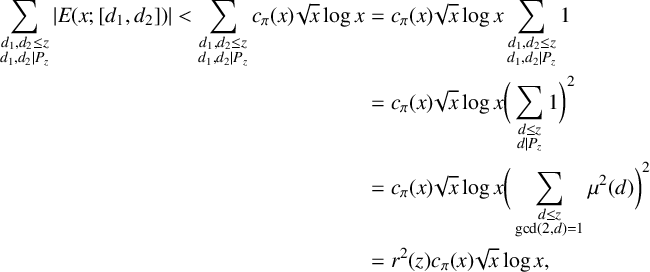$$ \begin{align*} \sum_{\substack{d_1, d_2 \leq z \\ d_1,d_2 | P_z}}{|E(x;[d_1,d_2])|} < \sum_{\substack{d_1, d_2 \leq z \\ d_1,d_2 | P_z}}{c_\pi(x)\sqrt{x}\log{x}}&= c_\pi(x)\sqrt{x}\log{x}\sum_{\substack{d_1, d_2 \leq z \\ d_1,d_2 | P_z}}{1} \\ &=c_\pi(x)\sqrt{x}\log{x}\bigg(\sum_{\substack{d \leq z \\ d| P_z}}{1}\bigg)^2 \\ &=c_\pi(x)\sqrt{x}\log{x}\bigg(\sum_{\substack{d \leq z \\ \gcd(2,d)=1}}{\mu^2(d)}\bigg)^2 \\ &=r^2(z)c_\pi(x)\sqrt{x}\log{x}, \end{align*} $$

by applying Lemma 2.4 on the second last line.

3 Upper bound on B

From [Reference Platt, Trudgian, Bailey, Borwein, Brent, Burachik, Osborn, Sims and Zhu11, Lemma 6],

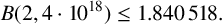$$ \begin{align*} B(2,4\cdot 10^{18})\leq 1.840\,518. \end{align*} $$

Now, using our bound on $\pi _2(x)$ , we can apply partial summation to calculate $B(m_1,\infty )$ . Let $z_i$ be fixed for each interval $[m_i,m_{i+1}]$ (the values of each $z_i$ and the intervals $[m_i,m_{i+1}]$ will be determined later).

Lemma 3.1. Assuming GRH, for $m_1 \geq 4\cdot 10^{18}$ and $z_i<m_i^{{1}/{4}}$ ,

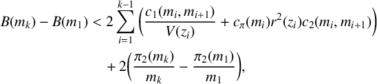$$ \begin{align*} B(m_k)-B(m_1) &< 2 \sum_{i=1}^{k-1}\bigg(\frac{c_1(m_i,m_{i+1})}{V(z_i)} + c_\pi(m_i)r^2(z_i)c_2(m_i,m_{i+1}) \bigg) \\ &\quad +2\bigg(\frac{\pi_2(m_k)}{m_k} -\frac{\pi_2(m_1)}{m_1} \bigg), \end{align*} $$

where

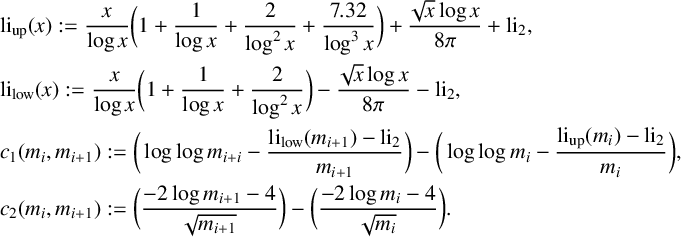$$ \begin{align*} &\mathrm{li}_{\mathrm{up}}(x) := \frac{x}{\log{x}}\bigg(1 + \frac{1}{\log{x}} + \frac{2}{\log^2{x}} + \frac{7.32}{\log^3{x}} \bigg) + \frac{\sqrt{x}\log{x}}{8\pi} + \mathrm{li}_2, \\ &\mathrm{li}_{\mathrm{low}}(x) := \frac{x}{\log{x}}\bigg(1 + \frac{1}{\log{x}} + \frac{2}{\log^2{x}} \bigg) - \frac{\sqrt{x}\log{x}}{8\pi} - \mathrm{li}_2, \\ & c_1(m_i,m_{i+1}) := \bigg(\log{\log{m_{i+i}}}- \frac{\mathrm{li}_{\mathrm{low}}(m_{i+1}) - \mathrm{li}_2}{m_{i+1}}\bigg) -\bigg(\log{\log{m_{i}}}- \frac{\mathrm{li}_{\mathrm{up}}(m_{i}) - \mathrm{li}_2}{m_{i}}\bigg),\\ & c_2(m_i,m_{i+1}) := \bigg( \frac{-2\log{m_{i+1}}-4}{\sqrt{m_{i+1}}} \bigg) - \bigg( \frac{-2\log{m_i}-4}{\sqrt{m_i}} \bigg). \end{align*} $$

Proof. We have

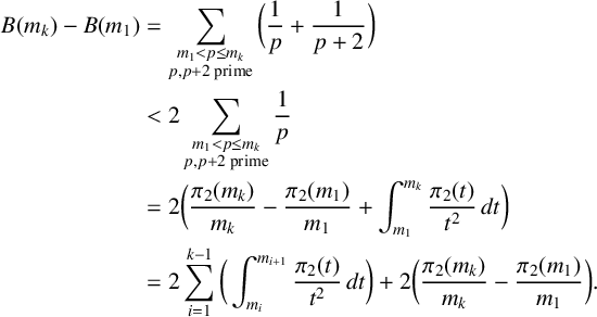$$ \begin{align*} B(m_k)-B(m_1) &= \sum_{\substack{m_1<p\leq m_k \\ p,p+2 \text{ prime}}}{\bigg(\frac{1}{p} + \frac{1}{p+2}\bigg)}\\ &< 2\sum_{\substack{m_1<p\leq m_k \\ p,p+2 \text{ prime}}}{\frac{1}{p}} \\ &=2\bigg(\frac{\pi_2(m_k)}{m_k} -\frac{\pi_2(m_1)}{m_1} + \int_{m_1}^{m_k}{\frac{\pi_2(t)}{t^2}}\,dt\bigg) \\ &=2\sum_{i=1}^{k-1}\bigg( \int_{m_i}^{m_{i+1}}{\frac{\pi_2(t)}{t^2}}\,dt \bigg) + 2\bigg(\frac{\pi_2(m_k)}{m_k} -\frac{\pi_2(m_1)}{m_1} \bigg). \end{align*} $$

The value of ${\pi _2(m_k)}/{m_k}$ will cancel in a further calculation, and the value of ${\pi _2(m_1)}/{m_1}$ can be calculated exactly using the computations performed by Oliveira e Silva [Reference Oliveira e Silva10]. For the remaining term, we proceed by

$$ \begin{align*} 2 \sum_{i=1}^{k-1}&\bigg( \int_{m_i}^{m_{i+1}}{\frac{\pi_2(t)}{t^2}} \,dt\bigg) < 2 \sum_{i=1}^{k-1}\bigg( \int_{m_i}^{m_{i+1}}{\frac{\mathrm{li}(t)}{V(z_i)\cdot t^2}}\,dt + \int_{m_i}^{m_{i+1}}{\frac{ r^2(z_i)c_\pi(t)\sqrt{t}\log{t}}{t^2}}\,dt \bigg). \end{align*} $$

We now apply some simplifications to these integrals to allow us to compute them analytically. Firstly, note that $V(z_i)$ and $r(z_i)$ are fixed for each interval $[m_i,m_{i+1}]$ . Also, note that $c_{\pi }(t)$ is monotonically decreasing and so $c_{\pi }(t) \leq c_{\pi }(m_i)$ for $x \in [m_i,m_{i+1}]$ . Consequently,

$$ \begin{align*} B(m_k)-B(m_i)<2 \sum_{i=1}^{k-1}\bigg( V(z_i)^{-1}\int_{m_i}^{m_{i+1}}{\frac{\mathrm{li}(t)}{t^2}}\,dt+ c_\pi(m_i)r^2(z_i)\int_{m_i}^{m_{i+1}}{\frac{ \sqrt{t}\log{t}}{t^2}}\,dt \bigg). \end{align*} $$

In computing the integral we note that

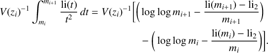$$ \begin{align*} V(z_i)^{-1}\int_{m_i}^{m_{i+1}}{\frac{\text{li}(t)}{t^2}}\,dt = V(z_i)^{-1}\bigg[\bigg(&\log{\log{m_{i+1}}}- \frac{\text{li}(m_{i+1}) - \text{li}_2}{m_{i+1}}\bigg)\\ & - \bigg(\log{\log{m_{i}}}- \frac{\text{li}(m_{i}) - \text{li}_2}{m_{i}}\bigg)\bigg]. \end{align*} $$

To avoid computing li $(x)$ directly, we use Schoenfeld’s bound on $|\pi (x)-\text {li}(x)|$ assuming the Riemann hypothesis [Reference Schoenfeld13, (6.18)], and Dusart’s bounds on $\pi (x)$ [Reference Dusart4, Theorem 5.1 and Corollary 5.2], to find (for $x \geq 4 \cdot 10^9$ ) that

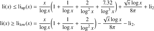$$ \begin{align*} \text{li}(x) \leq \text{li}_{\text{up}}(x) & = \frac{x}{\log{x}}\bigg(1 + \frac{1}{\log{x}} + \frac{2}{\log^2{x}} + \frac{7.32}{\log^3{x}} \bigg) + \frac{\sqrt{x}\log{x}}{8\pi} + \text{li}_2 \\ \text{li}(x) \geq \text{li}_{\text{low}}(x) & = \frac{x}{\log{x}}\bigg(1 + \frac{1}{\log{x}} + \frac{2}{\log^2{x}} \bigg) - \frac{\sqrt{x}\log{x}}{8\pi} - \text{li}_2. \end{align*} $$

And so

$$ \begin{align*} \int_{m_i}^{m_{i+1}}{\frac{\text{li}(t)}{t^2}}\,dt \leq &\bigg(\log{\log{m_{i+i}}}- \frac{\text{li}_{\text{low}}(m_{i+1}) - \text{li}_2}{m_{i+1}}\bigg) - \bigg(\log{\log{m_{i}}}- \frac{\text{li}_{\text{up}}(m_{i}) - \text{li}_2}{m_{i}}\bigg) \end{align*} $$

and finally,

$$ \begin{align*} c_\pi(m_i)r^2(z_i)\int_{m_i}^{m_{i+1}}{\frac{ \sqrt{t}\log{t}}{t^2}}\,dt = c_\pi(m_i)r^2(z_i) \bigg[\bigg( \frac{-2\log{m_{i+1}}-4}{\sqrt{m_{i+1}}} \bigg) - \bigg( \frac{-2\log{m_i}-4}{\sqrt{m_i}} \bigg)\bigg]. \end{align*} $$

Combining the above equations gives the desired result.

Lemma 3.2. We have

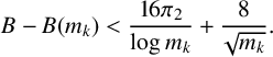(3.1) $$ \begin{align} B - B(m_k) < \frac{16 \pi_2}{\log{m_k}} + \frac{8}{\sqrt{m_k}}. \end{align} $$

Proof. We use [Reference Platt, Trudgian, Bailey, Borwein, Brent, Burachik, Osborn, Sims and Zhu11, Lemma 3] to bound the tail end of B, so that

$$ \begin{align*} B - B(m_k) \leq -2 \frac{\pi_2(m_k)}{m_k} + \int_{m_k}^{\infty}{\bigg(\frac{32 \pi_2}{t\log^2{t}} + 4t^{-{3}/{2}}\bigg)\,dt}=-2 \frac{\pi_2(m_k)}{m_k} +\frac{32 \pi_2}{\log{m_k}} + \frac{8}{\sqrt{m_k}}. \end{align*} $$

Combining the above two lemmas with [Reference Platt, Trudgian, Bailey, Borwein, Brent, Burachik, Osborn, Sims and Zhu11, Lemma 6] gives the following result.

Theorem 3.3. We have

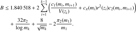$$ \begin{align*} B &\leq 1.840\,518 + 2 \sum_{i=1}^{k-1}\bigg(\frac{c_1(m_i,m_{i+1})}{V(z_i)} + c_\pi(m_i)r^2(z_i)c_2(m_i,m_{i+1}) \bigg) \\ &\quad + \frac{32 \pi_2}{\log{m_k}} + \frac{8}{\sqrt{m_k}} -2\frac{\pi_2(m_1)}{m_1}. \end{align*} $$

4 Calculating B

The final step is to determine the optimal parameters for the theorem. This involves selecting appropriate intervals $[m_i,m_{i+1}]$ and choosing corresponding values of $z_i$ for each interval. Generally, increasing the number of intervals reduces the overall error, though with diminishing returns as the interval size decreases. Based on this principle, we set $m_i \in \{4 \cdot 10^{18}\} \cup \{10^i: i = 19, 19.2, \ldots , 1999.8, 2000\}$ . To determine $z_i$ , we employ the Optim package in Julia [Reference Mogensen and Riseth8] to optimise $z_i$ within a specified domain. Since the optimal value of $z_i$ increases with i, we can restrict the search domain accordingly. Finally, all of the computations for B were performed using the IntervalArithmetic package in Julia [Reference Sanders and Benet12], ensuring rigorous explicit bounds.

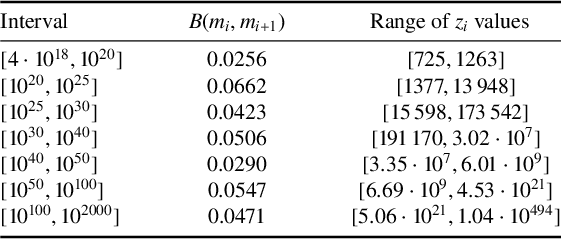
A subset of the optimised parameter ranges is presented in Table 1. The full set of intermediate calculations, along with the optimised values of $z_i$ for each interval, is available in the linked GitHub repository (https://github.com/LachlanJDunn/B_Under_GRH). This repository also includes the functions used to compute B and perform the parameter sweep. Additionally, it provides a method for estimating bounds on $B(a,b)$ for $4\cdot 10^{18} \leq m_1 \leq a < b \leq m_k$ , by computing $B(m_i,m_j)$ for the smallest interval that fully contains $[a,b]$ .

Table 1 $B(m_i,m_{i+1})$ for chosen intervals (rounded to 4 significant figures).

5 Potential improvements

We conclude by discussing several potential improvements to the presented method of bounding B.

• • As discussed earlier, splicing together different bounds for B over disjoint intervals could provide stronger estimates than restricting to only one method. The intermediate sums computed in this paper have been made available to facilitate this.

• • Computing $B(x_0)$ for a larger $x_0$ would reduce approximation errors, leading to a more precise bound.

• • Refining the choices of parameters $\{m_i\}$ and $\{z_i\}$ could potentially yield a more accurate result.