


1. Introduction
In shallow areas of the ocean, the seafloor may be subject to large oscillating pressure gradients and strong shear forces. This causes sediment to become suspended and transported to new locations, where it is deposited as the shear force oscillates. A model flow often used to investigate this process is the oscillatory boundary layer (OBL) problem. Stokes (Reference Stokes1855) was amongst the first to address this problem, specifically in the limit where viscous effects dominate and where the bottom surface is represented as a smooth flat wall. Under these assumptions, Stokes (Reference Stokes1855) derived analytical solutions that show the establishment of a boundary layer with characteristic thickness
 $\delta =\sqrt {2\nu /\omega }$
, where
$\delta =\sqrt {2\nu /\omega }$
, where
 $\nu$
is the fluid kinematic viscosity, and
$\nu$
is the fluid kinematic viscosity, and
 $\omega$
is the angular frequency of the oscillations. Due to the assumption of dominating viscous effects, these solutions apply only in the limit of very small Reynolds numbers
$\omega$
is the angular frequency of the oscillations. Due to the assumption of dominating viscous effects, these solutions apply only in the limit of very small Reynolds numbers
 ${\textit{Re}}_\delta =U_0 \delta /\nu$
, where
${\textit{Re}}_\delta =U_0 \delta /\nu$
, where
 $U_0$
is the velocity amplitude of the oscillations. Later, many researchers investigated the dynamics of OBLs over smooth and rough walls at larger Reynolds numbers, including when the Reynolds number is sufficiently high for turbulence to emerge (Hino, Sawamoto & Takasu Reference Hino, Sawamoto and Takasu1976; Akhavan et al. Reference Akhavan, Kamm and Shapiro1991b
; Sarpkaya Reference Sarpkaya1993; Vittori & Verzicco Reference Vittori and Verzicco1998; Costamagna, Vittori & Blondeaux Reference Costamagna, Vittori and Blondeaux2003; Salon, Armenio & Crise Reference Salon, Armenio and Crise2007; Carstensen et al. Reference Carstensen, Sumer and Fredsøe2010, Reference Carstensen, Sumer and Fredsøe2012; Pedocchi, Cantero & García Reference Pedocchi, Cantero and García2011; Ozdemir, Hsu & Balachandar Reference Ozdemir, Hsu and Balachandar2014; Ghodke & Apte Reference Ghodke and Apte2016, Reference Ghodke and Apte2018; Mazzuoli et al. Reference Mazzuoli, Kidanemariam, Blondeaux, Vittori and Uhlmann2016, Reference Mazzuoli, Blondeaux, Vittori, Uhlmann, Simeonov and Calantoni2020; Mazzuoli & Vittori Reference Mazzuoli and Vittori2019; Vittori et al. Reference Vittori, Blondeaux, Mazzuoli, Simeonov and Calantoni2020; Fytanidis, García & Fischer Reference Fytanidis, García and Fischer2021). However, it is unclear whether these results are applicable to seafloors. Unlike the previously studied configurations with impermeable and fixed smooth or rough walls, seafloors are made of sediment particles that together form a porous bed. Depending on the details of the flow over it, the bed may be static, with or without bedforms, and may even evolve dynamically as sediment particles saltate or become suspended by the flow (Finn, Li & Apte Reference Finn, Li and Apte2016). In this paper, we investigate how the dynamics of an OBL couple with those of a bottom collisional and freely evolving sediment bed at increasingly large Reynolds numbers.
$U_0$
is the velocity amplitude of the oscillations. Later, many researchers investigated the dynamics of OBLs over smooth and rough walls at larger Reynolds numbers, including when the Reynolds number is sufficiently high for turbulence to emerge (Hino, Sawamoto & Takasu Reference Hino, Sawamoto and Takasu1976; Akhavan et al. Reference Akhavan, Kamm and Shapiro1991b
; Sarpkaya Reference Sarpkaya1993; Vittori & Verzicco Reference Vittori and Verzicco1998; Costamagna, Vittori & Blondeaux Reference Costamagna, Vittori and Blondeaux2003; Salon, Armenio & Crise Reference Salon, Armenio and Crise2007; Carstensen et al. Reference Carstensen, Sumer and Fredsøe2010, Reference Carstensen, Sumer and Fredsøe2012; Pedocchi, Cantero & García Reference Pedocchi, Cantero and García2011; Ozdemir, Hsu & Balachandar Reference Ozdemir, Hsu and Balachandar2014; Ghodke & Apte Reference Ghodke and Apte2016, Reference Ghodke and Apte2018; Mazzuoli et al. Reference Mazzuoli, Kidanemariam, Blondeaux, Vittori and Uhlmann2016, Reference Mazzuoli, Blondeaux, Vittori, Uhlmann, Simeonov and Calantoni2020; Mazzuoli & Vittori Reference Mazzuoli and Vittori2019; Vittori et al. Reference Vittori, Blondeaux, Mazzuoli, Simeonov and Calantoni2020; Fytanidis, García & Fischer Reference Fytanidis, García and Fischer2021). However, it is unclear whether these results are applicable to seafloors. Unlike the previously studied configurations with impermeable and fixed smooth or rough walls, seafloors are made of sediment particles that together form a porous bed. Depending on the details of the flow over it, the bed may be static, with or without bedforms, and may even evolve dynamically as sediment particles saltate or become suspended by the flow (Finn, Li & Apte Reference Finn, Li and Apte2016). In this paper, we investigate how the dynamics of an OBL couple with those of a bottom collisional and freely evolving sediment bed at increasingly large Reynolds numbers.
There has been significant effort devoted to the characterisation of the boundary layer that develops over a smooth or rough wall under the action of an oscillatory forcing. Depending on the Reynolds number
 ${\textit{Re}}_{\delta }$
, different regimes have been identified (as detailed in Akhavan et al. Reference Akhavan, Kamm and Shapiro1991a
; Vittori & Verzicco Reference Vittori and Verzicco1998; Pedocchi et al. Reference Pedocchi, Cantero and García2011; Ozdemir et al. Reference Ozdemir, Hsu and Balachandar2014; Fytanidis et al. Reference Fytanidis, García and Fischer2021). To summarise, an OBL developing over an impermeable wall may exhibit four different regimes. The laminar regime occurs in smooth, rough and wavy wall OBLs at
${\textit{Re}}_{\delta }$
, different regimes have been identified (as detailed in Akhavan et al. Reference Akhavan, Kamm and Shapiro1991a
; Vittori & Verzicco Reference Vittori and Verzicco1998; Pedocchi et al. Reference Pedocchi, Cantero and García2011; Ozdemir et al. Reference Ozdemir, Hsu and Balachandar2014; Fytanidis et al. Reference Fytanidis, García and Fischer2021). To summarise, an OBL developing over an impermeable wall may exhibit four different regimes. The laminar regime occurs in smooth, rough and wavy wall OBLs at
 ${\textit{Re}}_\delta \lesssim 85$
. In this regime, the flow is laminar throughout the oscillation cycle (Blondeaux & Seminara Reference Blondeaux and Seminara1979; Akhavan et al. Reference Akhavan, Kamm and Shapiro1991a
; Vittori & Verzicco Reference Vittori and Verzicco1998), and is well described by the analytical solutions of Stokes (Reference Stokes1855). For
${\textit{Re}}_\delta \lesssim 85$
. In this regime, the flow is laminar throughout the oscillation cycle (Blondeaux & Seminara Reference Blondeaux and Seminara1979; Akhavan et al. Reference Akhavan, Kamm and Shapiro1991a
; Vittori & Verzicco Reference Vittori and Verzicco1998), and is well described by the analytical solutions of Stokes (Reference Stokes1855). For
 $85\lesssim {\textit{Re}}_\delta \lesssim 550$
, the flow is in the disturbed laminar regime (Hino et al. Reference Hino, Sawamoto and Takasu1976; Jensen, Sumer & Fredsøe Reference Jensen, Sumer and Fredsøe1989). The latter is characterised by the appearance of small-amplitude perturbations superimposed upon the Stokes flow (Vittori & Verzicco Reference Vittori and Verzicco1998). Fytanidis et al. (Reference Fytanidis, García and Fischer2021) found that the Reynolds number thresholds for this regime depend strongly on background disturbances. For
$85\lesssim {\textit{Re}}_\delta \lesssim 550$
, the flow is in the disturbed laminar regime (Hino et al. Reference Hino, Sawamoto and Takasu1976; Jensen, Sumer & Fredsøe Reference Jensen, Sumer and Fredsøe1989). The latter is characterised by the appearance of small-amplitude perturbations superimposed upon the Stokes flow (Vittori & Verzicco Reference Vittori and Verzicco1998). Fytanidis et al. (Reference Fytanidis, García and Fischer2021) found that the Reynolds number thresholds for this regime depend strongly on background disturbances. For
 $550\lesssim {\textit{Re}}_\delta \lesssim 3460$
, the flow enters the intermittent turbulent regime, and is characterised by sudden turbulence eruption during the decelerating portion of the oscillatory period before relaminarising again. Finally, the turbulent regime occurs for
$550\lesssim {\textit{Re}}_\delta \lesssim 3460$
, the flow enters the intermittent turbulent regime, and is characterised by sudden turbulence eruption during the decelerating portion of the oscillatory period before relaminarising again. Finally, the turbulent regime occurs for
 ${\textit{Re}}_\delta \gtrsim 3460$
. In this regime, Jensen et al. (Reference Jensen, Sumer and Fredsøe1989) show that the OBL presents sustained velocity fluctuations and a logarithmic layer for at least 90 % of the cycle.
${\textit{Re}}_\delta \gtrsim 3460$
. In this regime, Jensen et al. (Reference Jensen, Sumer and Fredsøe1989) show that the OBL presents sustained velocity fluctuations and a logarithmic layer for at least 90 % of the cycle.
Note that with a bottom rough wall, the Reynolds number thresholds between the different regimes may vary considerably, as the flow characteristics depend on additional roughness parameters, such as the Keulegan–Carpenter number
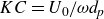
 $KC = U_0/(\omega d_{\!p})$
, where
$KC = U_0/(\omega d_{\!p})$
, where
 $d_{\!p}$
represents the roughness size. Jensen et al. (Reference Jensen, Sumer and Fredsøe1989) showed that disturbances caused by fixed sandpaper roughness lead to a thicker boundary layer and increased turbulence intensity. Similarly, Xiong et al. (Reference Xiong, Qi, Gao, Xu, Ren and Cheng2020) found that a flow disturbance created by a wall-mounted obstacle leads to earlier transition to turbulence, thereby lowering the threshold
$d_{\!p}$
represents the roughness size. Jensen et al. (Reference Jensen, Sumer and Fredsøe1989) showed that disturbances caused by fixed sandpaper roughness lead to a thicker boundary layer and increased turbulence intensity. Similarly, Xiong et al. (Reference Xiong, Qi, Gao, Xu, Ren and Cheng2020) found that a flow disturbance created by a wall-mounted obstacle leads to earlier transition to turbulence, thereby lowering the threshold
 ${\textit{Re}}_\delta$
compared to that found for a smooth wall OBL. Additional studies of roughness effects can be found in Ghodke & Apte (Reference Ghodke and Apte2016, Reference Ghodke and Apte2018) and Mazzuoli & Vittori (Reference Mazzuoli and Vittori2019).
${\textit{Re}}_\delta$
compared to that found for a smooth wall OBL. Additional studies of roughness effects can be found in Ghodke & Apte (Reference Ghodke and Apte2016, Reference Ghodke and Apte2018) and Mazzuoli & Vittori (Reference Mazzuoli and Vittori2019).
Permeability may also have a significant effect on the structure of an OBL developing over a particle bed. Conley & Inman (Reference Conley and Inman1994) performed experiments with a ventilated OBL, i.e. an OBL with periodic transpiration over a permeable wall. They found that the wall shear stress decreases during suction and increases during injection. For a permeable wall, the no-slip condition may no longer hold, as observed by Liu, Davis & Downing (Reference Liu, Davis and Downing1996) and Breugem, Boersma & Uittenbogaard (Reference Breugem, Boersma and Uittenbogaard2006). By comparing simulations of an OBL with experimental data, Meza-Valle & Pujara (Reference Meza-Valle and Pujara2022) showed that a mixed boundary condition at the surface best captures the flow over a permeable wall. A permeable bed allows flow penetration, which in turn creates a Kelvin–Helmholtz instability and an inflection point in the fluid velocity within the boundary layer (Sparrow et al. Reference Sparrow and Pokrajac2012; Voermans, Ghisalberti & Ivey Reference Voermans, Ghisalberti and Ivey2017). All these modifications caused by the bed permeability make it difficult to estimate the bed shear stress beforehand (Yuan & Madsen Reference Yuan and Madsen2014).
The studies discussed thus far considered fixed porous beds. In the case of mobile beds, particle transport may further alter the bed–fluid interface. Particle motion leads to the emergence of new regimes, as discussed by Finn & Li (Reference Finn and Li2016), who proposed a regime map for sediment–turbulent interactions. In the no-motion regime, the bed remains stationary and acts as previously described. In the bedform regime, ripples emerge in the particle bed as particles saltate over the surface. The study of Mazzuoli, Kidanemariam & Uhlmann (Reference Mazzuoli, Kidanemariam and Uhlmann2019), by means of particle-resolved direct numerical simulations (PR-DNS), illustrates this regime. The authors showed the emergence of rolling-grain ripples in an OBL developing over a sediment bed at
 ${\textit{Re}}_\delta \sim 100$
, density ratio
${\textit{Re}}_\delta \sim 100$
, density ratio
 $\rho _{\!p}/\rho _{\!f}\sim 2.5$
, and Galileo number
$\rho _{\!p}/\rho _{\!f}\sim 2.5$
, and Galileo number
 ${\textit{Ga}}\sim 10$
. The latter represents the relative effect of gravitational and viscous forces exerted on sediment grains. An earlier study showed that ripples emerge from the interaction between particle rows and recirculation zones in the OBL (Mazzuoli et al. Reference Mazzuoli, Kidanemariam, Blondeaux, Vittori and Uhlmann2016). In the sheet flow regime, the bed–fluid interface recedes due to the formation of a layer of suspended particles (Hsu, Jenkins & Liu Reference Hsu, Jenkins and Liu2004; O’Donoghue & Wright Reference O’Donoghue and Wright2004). Mazzuoli et al. (Reference Mazzuoli, Blondeaux, Vittori, Uhlmann, Simeonov and Calantoni2020) showed that the eruption of turbulence plays a role in the sediment resuspension. Further, at relatively low values of the Shields number, sediment transport may depend on both Shields number and flow acceleration.
${\textit{Ga}}\sim 10$
. The latter represents the relative effect of gravitational and viscous forces exerted on sediment grains. An earlier study showed that ripples emerge from the interaction between particle rows and recirculation zones in the OBL (Mazzuoli et al. Reference Mazzuoli, Kidanemariam, Blondeaux, Vittori and Uhlmann2016). In the sheet flow regime, the bed–fluid interface recedes due to the formation of a layer of suspended particles (Hsu, Jenkins & Liu Reference Hsu, Jenkins and Liu2004; O’Donoghue & Wright Reference O’Donoghue and Wright2004). Mazzuoli et al. (Reference Mazzuoli, Blondeaux, Vittori, Uhlmann, Simeonov and Calantoni2020) showed that the eruption of turbulence plays a role in the sediment resuspension. Further, at relatively low values of the Shields number, sediment transport may depend on both Shields number and flow acceleration.
Several computational methods can be leveraged to study the dynamics of an OBL over a sediment bed. The PR-DNS, in which the boundary layer around each sediment grain is fully resolved, provides the highest fidelity since it requires little to no modelling (Uhlmann Reference Uhlmann2005; Apte, Martin & Patankar Reference Apte, Martin and Patankar2009; Breugem Reference Breugem2012; Kempe & Fröhlich Reference Kempe and Fröhlich2012; Kasbaoui & Herrmann Reference Kasbaoui and Herrmann2025). However, this results in very high computational cost, as seen from the PR-DNS of Mazzuoli et al. (Reference Mazzuoli, Kidanemariam and Uhlmann2019). While using smaller computational domains and shorter integration times may reduce computational cost, it also introduces numerical artefacts. For example, the domain considered in the PR-DNS of Mazzuoli et al. (Reference Mazzuoli, Blondeaux, Vittori, Uhlmann, Simeonov and Calantoni2020) was too small to allow the natural formation of ripples in the sediment bed. Even with this restrictive domain size, the high cost of the PR-DNS of Mazzuoli et al. (Reference Mazzuoli, Blondeaux, Vittori, Uhlmann, Simeonov and Calantoni2020) limited the integration time to the first 1–4 cycles of the OBL, which may not be enough to reach a statistically quasi-periodic state. In contrast, the Euler–Lagrange method provides a good balance between computational cost and fidelity (Capecelatro & Desjardins Reference Capecelatro and Desjardins2013a ; Finn et al. Reference Finn, Li and Apte2016). In this approach, flow features and bed dynamics on scales larger than the particle size are well resolved, while the flow on the scale of the particle is modelled. This makes it possible to simulate the dynamics on length and time scales much larger than those accessible in PR-DNS. Earlier studies showed that this approach can reproduce with high fidelity the dynamics of dense fluidised beds (Capecelatro & Desjardins Reference Capecelatro and Desjardins2013a ) and dense slurries (Capecelatro & Desjardins Reference Capecelatro and Desjardins2013b ; Arolla & Desjardins Reference Arolla and Desjardins2015), including in sheet flow and bedform regimes. More recently, Rao & Capecelatro (Reference Rao and Capecelatro2019) showed that predictions with the Euler–Lagrange method for the evolution of sediment bed under both laminar and turbulent shear flow match very well with PR-DNS (Kidanemariam & Uhlmann Reference Kidanemariam and Uhlmann2014) and experiments (Aussillous et al. Reference Aussillous, Chauchat, Pailha, Médale and Guazzelli2013).
In this paper, we study the interplay between an OBL and a sediment bed made of collisional and freely evolving particles from the laminar regime to the onset of turbulence using Euler–Lagrange simulations. The structure of the paper is as follows. In § 2, we provide the governing equations that dictate the evolution of the flow and sediment particles. In § 3, we provide details on the computations and parameters used in this study. Next, we analyse statistics of the fluid and solid phases in § 4, highlighting how sediment bed dynamics couple with those of the OBL. Finally, we give concluding remarks in § 5.
2. Governing equations
We use the volume-filtering approach of Anderson & Jackson (Reference Anderson and Jackson1967) and the Euler–Lagrange methodology of Capecelatro & Desjardins (Reference Capecelatro and Desjardins2013a
) to describe the dynamics of the sediment-laden flow. The carrier phase is an incompressible fluid with density
 $\rho _{\!f}$
and viscosity
$\rho _{\!f}$
and viscosity
 $\mu _{\!f}$
. The volume-filtered Navier–Stokes equations read
$\mu _{\!f}$
. The volume-filtered Navier–Stokes equations read
 \begin{align} \frac {\partial }{\partial t} (\alpha _{\!f} \rho _{\!f})+\boldsymbol{\nabla }\boldsymbol{\cdot }(\alpha _{\!f} \rho _{\!f} \boldsymbol{u}_{\!f}) &= 0 , \end{align}
 \begin{align} \frac {\partial }{\partial t}(\alpha _{\!f} {\rho _{\!f}} \boldsymbol{u}_{\!f})+\boldsymbol{\nabla }\boldsymbol{\cdot }(\alpha _{\!f} {\rho _{\!f}} \boldsymbol{u}_{\!f} \boldsymbol{u}_{\!f}) &= \boldsymbol{\nabla }\boldsymbol{\cdot }\left (\boldsymbol{\tau } + \boldsymbol{R}_{\mu }\right )+\alpha _{\!f} {\rho _{\!f}} \boldsymbol{g} - \boldsymbol{F}_{\!p}+ \boldsymbol{A}, \end{align}
where
 $\alpha _{\!f}$
is the fluid volume fraction,
$\alpha _{\!f}$
is the fluid volume fraction,
 $\boldsymbol{u}_{\!f}$
is the volume-filtered fluid velocity,
$\boldsymbol{u}_{\!f}$
is the volume-filtered fluid velocity,
 ${\boldsymbol{\tau }}=-p\boldsymbol{I}+\mu [\boldsymbol{\nabla }\boldsymbol{u}_{\!f}+\boldsymbol{\nabla }\boldsymbol{u}_{\!f}^{\rm T}-( {2}/{3})(\boldsymbol{\nabla }\boldsymbol{\cdot }\boldsymbol{u}_{\!f})\boldsymbol{I}]$
is the resolved fluid stress tensor (Capecelatro & Desjardins Reference Capecelatro and Desjardins2013a
),
${\boldsymbol{\tau }}=-p\boldsymbol{I}+\mu [\boldsymbol{\nabla }\boldsymbol{u}_{\!f}+\boldsymbol{\nabla }\boldsymbol{u}_{\!f}^{\rm T}-( {2}/{3})(\boldsymbol{\nabla }\boldsymbol{\cdot }\boldsymbol{u}_{\!f})\boldsymbol{I}]$
is the resolved fluid stress tensor (Capecelatro & Desjardins Reference Capecelatro and Desjardins2013a
),
 $p$
is pressure, which includes the hydrostatic contribution,
$p$
is pressure, which includes the hydrostatic contribution,
 $\boldsymbol{g}$
is the gravitational acceleration, and
$\boldsymbol{g}$
is the gravitational acceleration, and
 $\boldsymbol{F}_{\!p}$
is the momentum exchange between the particles and the fluid. The tensor
$\boldsymbol{F}_{\!p}$
is the momentum exchange between the particles and the fluid. The tensor
 $\boldsymbol{R}_{\mu }$
represents the so-called residual viscous stress tensor. This term arises from filtering the pointwise stress tensor. It includes sub-filter scale terms that require closure. This term is believed to be responsible for the apparent enhanced viscosity observed in viscous fluids containing suspended solid particles. For this reason, Capecelatro & Desjardins (Reference Capecelatro and Desjardins2013a
) proposed a closure using an effective viscosity, which, when combined with the effective viscosity model of Gibilaro et al. (Reference Gibilaro, Gallucci, Di Felice and Pagliai2007), leads to an expression for the residual viscous stress tensor:
$\boldsymbol{R}_{\mu }$
represents the so-called residual viscous stress tensor. This term arises from filtering the pointwise stress tensor. It includes sub-filter scale terms that require closure. This term is believed to be responsible for the apparent enhanced viscosity observed in viscous fluids containing suspended solid particles. For this reason, Capecelatro & Desjardins (Reference Capecelatro and Desjardins2013a
) proposed a closure using an effective viscosity, which, when combined with the effective viscosity model of Gibilaro et al. (Reference Gibilaro, Gallucci, Di Felice and Pagliai2007), leads to an expression for the residual viscous stress tensor:
 \begin{equation} \boldsymbol{R}_{\mu } = \mu _{\!f}(\alpha _{\!f}^{-2.8}-1)\bigg[\boldsymbol{\nabla }\boldsymbol{u}_{\!f}+\boldsymbol{\nabla }\boldsymbol{u}_{\!f}^{\rm T}-\dfrac {2}{3}(\boldsymbol{\nabla }\boldsymbol{\cdot }\boldsymbol{u}_{\!f})\boldsymbol{I}\bigg]. \end{equation}
We do not use an eddy viscosity model since none of the cases that we discuss here leads to fully developed turbulence.
In order to study the dynamics of an OBL, we drive the flow using the last term in (2.2), expressed as
 \begin{equation} \boldsymbol{A} = \alpha _{\!f} \rho _{\!f} U_0 \omega \cos (\omega t)\,\boldsymbol{e}_x. \end{equation}
This represents a harmonic pressure gradient forcing with angular frequency
 $\omega$
and velocity amplitude
$\omega$
and velocity amplitude
 $U_0$
. Here,
$U_0$
. Here,
 $x$
is the coordinate in the streamwise direction along the unitary vector
$x$
is the coordinate in the streamwise direction along the unitary vector
 $\boldsymbol{e}_x$
,
$\boldsymbol{e}_x$
,
 $y$
is the coordinate in the wall-normal direction, and
$y$
is the coordinate in the wall-normal direction, and
 $z$
is the coordinate in the spanwise direction.
$z$
is the coordinate in the spanwise direction.
The particles are described in the Lagrangian frame. Following Maxey & Riley (Reference Maxey and Riley1983), the equations of motion of a particle
 $i$
are given by
$i$
are given by
 \begin{align} \frac {{\rm d} \boldsymbol{x}^i_{\!p}}{{\rm d} t}(t) &= \boldsymbol{u}^i_{\!p}(t), \end{align}
 \begin{align} m_{\!p} \frac {{\rm d} \boldsymbol{u}^i_{\!p}}{{\rm d} t}(t) &= {\boldsymbol{f}^{h,i}_{\!p} + \boldsymbol{f}^{c,i}_{\!p}}, \end{align}
 \begin{align} {I_{\!p} \frac {{\rm d} \boldsymbol{\omega }^i_{\!p}}{{\rm d} t}(t)} &= {\boldsymbol{T}_{\!p}^{c,i}}, \end{align}
where
 $\boldsymbol{x}^{i}_{\!p}$
,
$\boldsymbol{x}^{i}_{\!p}$
,
 $\boldsymbol{u}^{i}_{\!p}$
,
$\boldsymbol{u}^{i}_{\!p}$
,
 $\boldsymbol{\omega }^{i}_{\!p}$
,
$\boldsymbol{\omega }^{i}_{\!p}$
,
 $m_{\!p}$
and
$m_{\!p}$
and
 $I_{\!p}$
are the particle position, velocity, angular velocity, mass and moment of inertia, respectively. Here,
$I_{\!p}$
are the particle position, velocity, angular velocity, mass and moment of inertia, respectively. Here,
 $\boldsymbol{f}^{h,i}_{\!p}$
represents the hydrodynamic force, which is modelled as (Van Doren & Kasbaoui Reference Van Doren and Kasbaoui2024)
$\boldsymbol{f}^{h,i}_{\!p}$
represents the hydrodynamic force, which is modelled as (Van Doren & Kasbaoui Reference Van Doren and Kasbaoui2024)
 \begin{equation} {\boldsymbol{f}^{h,i}_{\!p}(t) = V_{\!p} \left .\boldsymbol{\nabla }\boldsymbol{\cdot }\boldsymbol{\tau }\right |_{\boldsymbol{x}_{\!p}^i} + m_{\!p} f_d\frac {\boldsymbol{u}_{\!f}(\boldsymbol{x}^i_{\!p},t)-\boldsymbol{u}^i_{\!p}}{\tau _{\!p}} + \boldsymbol{f}_{\!p}^{{am},i} + \boldsymbol{f}_{\!p}^{{lift}, i}, } \end{equation}
where
 $V_{\!p} = \pi d^{3}_{\!p}/6$
is the particle volume. The first term on the right-hand side of (2.8) represents the effect of the undisturbed flow field (Maxey & Riley Reference Maxey and Riley1983). The second term represents the drag force exerted on a particle. Note that
$V_{\!p} = \pi d^{3}_{\!p}/6$
is the particle volume. The first term on the right-hand side of (2.8) represents the effect of the undisturbed flow field (Maxey & Riley Reference Maxey and Riley1983). The second term represents the drag force exerted on a particle. Note that
 $\tau _{\!p}=\rho _{\!p} d_{\!p}^2/(18\mu )$
is the particle response time, and
$\tau _{\!p}=\rho _{\!p} d_{\!p}^2/(18\mu )$
is the particle response time, and
 $f_d$
is a drag correction factor. We use the one by Tenneti, Garg & Subramaniam (Reference Tenneti, Garg and Subramaniam2011), derived from PR-DNS, which accounts for both inertial and high particle volume fraction effects. The last two terms on the right-hand side of (2.8) represent the added mass and Saffman lift (Saffman Reference Saffman1965) forces,
$f_d$
is a drag correction factor. We use the one by Tenneti, Garg & Subramaniam (Reference Tenneti, Garg and Subramaniam2011), derived from PR-DNS, which accounts for both inertial and high particle volume fraction effects. The last two terms on the right-hand side of (2.8) represent the added mass and Saffman lift (Saffman Reference Saffman1965) forces,
 \begin{align} \boldsymbol{f}_{\!p}^{ {am},i}&=\frac {1}{2} \alpha _{\!f} \rho _{\!f} V_{\!p} \left (\frac {{\rm D} \boldsymbol{u}_{\!f}(\boldsymbol{x}^i_{\!p},t)}{{\rm D}t} -\frac {{\rm d} \boldsymbol{u}_{\!p}^i}{{\rm d}t}\right ), \end{align}
 \begin{align} \boldsymbol{f}_{\!p}^{ {lift},i} &= 1.615 J \mu _{\!f} d_{\!p}\, |\boldsymbol{u}^i_{s}|\,\sqrt {\frac {d_{\!p}^2\, |\boldsymbol{\omega }^i|\, \alpha _{\!f}\rho _{\!f} }{\mu _{\!f}}} \frac { \boldsymbol{u}^i_{s}\times \boldsymbol{\omega }^i}{|\boldsymbol{u}^i_{s}|\, |\boldsymbol{\omega }^i|}, \end{align}
where
 $\boldsymbol{\omega }^i = \boldsymbol{\omega }_{\!f}(\boldsymbol{x^i_{\!p}},t)$
is the fluid vorticity at the particle location,
$\boldsymbol{\omega }^i = \boldsymbol{\omega }_{\!f}(\boldsymbol{x^i_{\!p}},t)$
is the fluid vorticity at the particle location,
 $\boldsymbol{u}^i_{s} = \boldsymbol{u}_{\!f}(\boldsymbol{x}^i_{\!p},t) - \boldsymbol{u}^i_{\!p}$
is the slip velocity, and
$\boldsymbol{u}^i_{s} = \boldsymbol{u}_{\!f}(\boldsymbol{x}^i_{\!p},t) - \boldsymbol{u}^i_{\!p}$
is the slip velocity, and
 $J$
is a lift correction, which is equal to 1 in the model from Saffman (Reference Saffman1965).
$J$
is a lift correction, which is equal to 1 in the model from Saffman (Reference Saffman1965).
The term
 $\boldsymbol{f}_{\!p}^{c,i}$
represents the collisional force exerted on the particle due to particle–particle and particle–wall collisions. These collisions are modelled using the soft-sphere model, as detailed in Capecelatro & Desjardins (Reference Capecelatro and Desjardins2013a
). Briefly, the force exerted on particle
$\boldsymbol{f}_{\!p}^{c,i}$
represents the collisional force exerted on the particle due to particle–particle and particle–wall collisions. These collisions are modelled using the soft-sphere model, as detailed in Capecelatro & Desjardins (Reference Capecelatro and Desjardins2013a
). Briefly, the force exerted on particle
 $a$
due to a collision with particle
$a$
due to a collision with particle
 $b$
, denoted
$b$
, denoted
 $\boldsymbol{f}_{\!p}^{{c,b\rightarrow a}}$
, is decomposed into normal and tangential components. The normal component
$\boldsymbol{f}_{\!p}^{{c,b\rightarrow a}}$
, is decomposed into normal and tangential components. The normal component
 $\boldsymbol{f}_{p,n}^{{c,b\rightarrow a}}$
is modelled as a linearised spring–dashpot system, i.e.
$\boldsymbol{f}_{p,n}^{{c,b\rightarrow a}}$
is modelled as a linearised spring–dashpot system, i.e.
 \begin{equation} \boldsymbol{f}_{p,n}^{{c,b\rightarrow a}} = \begin{cases} -k\delta _{ab} \boldsymbol{n}_{ab}-\eta \boldsymbol{u}_{ab,n} & \text{if } \left|\boldsymbol{x}_{\!p}^a-\boldsymbol{x}_{\!p}^b\right| \lt 0.5\left(d_{\!p}^a+d_{\!p}^b\right)+\lambda, \\[6pt] 0 & \textrm {otherwise}, \end{cases} \end{equation}
where
 $\delta _{ab}= 0.5(d_{\!p}^a+d_{\!p}^b)-|\boldsymbol{x}_{\!p}^a-\boldsymbol{x}_{\!p}^b|$
is the overlap between particles
$\delta _{ab}= 0.5(d_{\!p}^a+d_{\!p}^b)-|\boldsymbol{x}_{\!p}^a-\boldsymbol{x}_{\!p}^b|$
is the overlap between particles
 $a$
and
$a$
and
 $b$
,
$b$
,
 $\boldsymbol{n}_{ab}$
is the unit normal vector between the particles, and
$\boldsymbol{n}_{ab}$
is the unit normal vector between the particles, and
 $\boldsymbol{u}_{ab,n}$
is the normal relative velocity. The parameters
$\boldsymbol{u}_{ab,n}$
is the normal relative velocity. The parameters
 $k$
and the
$k$
and the
 $\eta$
are the spring stiffness and damping factor, respectively.
$\eta$
are the spring stiffness and damping factor, respectively.
Note that the governing equations (2.1) and (2.2) for the fluid phase are solved in both simulations with particles and without. In the latter case,
 $\alpha _{\!f}=1$
throughout the domain, which recovers the standard Navier–Stokes equations.
$\alpha _{\!f}=1$
throughout the domain, which recovers the standard Navier–Stokes equations.
The solid phase dynamics is coupled with the fluid phase dynamics through the momentum exchange field
 $\boldsymbol{F}_{\!p}$
, and the volume fraction fields,
$\boldsymbol{F}_{\!p}$
, and the volume fraction fields,
 $\alpha _{\!f}$
and
$\alpha _{\!f}$
and
 $\alpha _{\!p}$
. We calculate these fields using
$\alpha _{\!p}$
. We calculate these fields using
 \begin{align} \boldsymbol{F}_{\!p}(\boldsymbol{x},t) &= \sum _{i=1}^N \boldsymbol{f}^{h,i}_{\!p}(t)\, g(\|\boldsymbol{x}-\boldsymbol{x}^i_{\!p}\|), \end{align}
 \begin{align} \alpha _{\!p}(\boldsymbol{x},t) &= \sum _{i=1}^{N} V_{\!p}\, g(\|\boldsymbol{x}-\boldsymbol{x}^i_{\!p}\|), \end{align}
 \begin{align} \alpha _{\!f}(\boldsymbol{x},t) &= 1 - \alpha _{\!p}(\boldsymbol{x},t). \end{align}
In these equations,
 $g$
represents a Gaussian filter with width
$g$
represents a Gaussian filter with width
 $\delta _{\!f} = 5 d_{\!p}$
. We study the influence of filter width on fluid statistics in Appendix A, and show that the statistics are converged with respect to filter width at
$\delta _{\!f} = 5 d_{\!p}$
. We study the influence of filter width on fluid statistics in Appendix A, and show that the statistics are converged with respect to filter width at
 $\delta _{\!f} = 5 d_{\!p}$
. Additional details on the computation of these terms and validation of the computational strategy, can be found in Capecelatro & Desjardins (Reference Capecelatro and Desjardins2013a
,
Reference Capecelatro and Desjardinsb
), Capecelatro, Pepiot & Desjardins (Reference Capecelatro, Pepiot and Desjardins2014) and Rao & Capecelatro (Reference Rao and Capecelatro2019), and in our recent work (Kasbaoui Reference Kasbaoui2019; Kasbaoui, Koch & Desjardins Reference Kasbaoui, Koch and Desjardins2019; Shuai & Kasbaoui Reference Shuai and Kasbaoui2022; Shuai et al. Reference Shuai, Dhas, Roy and Kasbaoui2022; Dave & Kasbaoui Reference Dave and Kasbaoui2023; Shuai, Roy & Kasbaoui Reference Shuai, Roy and Kasbaoui2024; Van Doren & Kasbaoui Reference Van Doren and Kasbaoui2024). In Appendix D, we further demonstrate the ability of this approach to capture sediment transport accurately. This is done by comparing sediment flow rates obtained with this method in laminar channel flows at varying Shields numbers with those obtained from PR-DNS (Kidanemariam & Uhlmann Reference Kidanemariam and Uhlmann2014) and laboratory experiments (Aussillous et al. Reference Aussillous, Chauchat, Pailha, Médale and Guazzelli2013). Based on the excellent agreement shown in Appendix D, we conclude that this Euler–Lagrange method is well suited for this study.
$\delta _{\!f} = 5 d_{\!p}$
. Additional details on the computation of these terms and validation of the computational strategy, can be found in Capecelatro & Desjardins (Reference Capecelatro and Desjardins2013a
,
Reference Capecelatro and Desjardinsb
), Capecelatro, Pepiot & Desjardins (Reference Capecelatro, Pepiot and Desjardins2014) and Rao & Capecelatro (Reference Rao and Capecelatro2019), and in our recent work (Kasbaoui Reference Kasbaoui2019; Kasbaoui, Koch & Desjardins Reference Kasbaoui, Koch and Desjardins2019; Shuai & Kasbaoui Reference Shuai and Kasbaoui2022; Shuai et al. Reference Shuai, Dhas, Roy and Kasbaoui2022; Dave & Kasbaoui Reference Dave and Kasbaoui2023; Shuai, Roy & Kasbaoui Reference Shuai, Roy and Kasbaoui2024; Van Doren & Kasbaoui Reference Van Doren and Kasbaoui2024). In Appendix D, we further demonstrate the ability of this approach to capture sediment transport accurately. This is done by comparing sediment flow rates obtained with this method in laminar channel flows at varying Shields numbers with those obtained from PR-DNS (Kidanemariam & Uhlmann Reference Kidanemariam and Uhlmann2014) and laboratory experiments (Aussillous et al. Reference Aussillous, Chauchat, Pailha, Médale and Guazzelli2013). Based on the excellent agreement shown in Appendix D, we conclude that this Euler–Lagrange method is well suited for this study.
3. Numerical experiments
3.1. Configuration
We consider the dynamics of an OBL over a cohesionless particle bed at three Reynolds numbers,
 ${\textit{Re}}_\delta =200$
, 400 and 800. A summary of the relevant non-dimensional parameters for each run is given in table 1. In order to provide a baseline for comparisons with the sediment-laden cases, we also carry out companion simulations at the same Reynolds numbers but with a bottom smooth and impermeable wall instead of a particle bed (see Appendix A). Note that without the particle bed, the flow at
${\textit{Re}}_\delta =200$
, 400 and 800. A summary of the relevant non-dimensional parameters for each run is given in table 1. In order to provide a baseline for comparisons with the sediment-laden cases, we also carry out companion simulations at the same Reynolds numbers but with a bottom smooth and impermeable wall instead of a particle bed (see Appendix A). Note that without the particle bed, the flow at
 ${\textit{Re}}_\delta =200$
and 400 is in the laminar regime (see Appendix A). We do not observe a disturbed laminar regime in these simulations due to the wall being smooth and flat, and the absence of any external disturbances. Without small pertubations, the disturbed laminar regime would take much longer to emerge than the simulations that we performed. The flow at
${\textit{Re}}_\delta =200$
and 400 is in the laminar regime (see Appendix A). We do not observe a disturbed laminar regime in these simulations due to the wall being smooth and flat, and the absence of any external disturbances. Without small pertubations, the disturbed laminar regime would take much longer to emerge than the simulations that we performed. The flow at
 ${\textit{Re}}_\delta =800$
falls in the intermittent turbulent regime. Comparing the simulations with and without a bottom particle bed helps to elucidate the impact of sediment motion, bedforms and bed permeability on the flow statistics.
${\textit{Re}}_\delta =800$
falls in the intermittent turbulent regime. Comparing the simulations with and without a bottom particle bed helps to elucidate the impact of sediment motion, bedforms and bed permeability on the flow statistics.
Table 1. Summary of the non-dimensional parameters for the present runs of an OBL over a sediment bed. The maximum Shields number is determined a priori from the smooth wall shear stress as described in § 4.2.

In addition to the Reynolds number
 ${\textit{Re}}_\delta$
, the presence of particles introduces additional dimensionless parameters. These are:
${\textit{Re}}_\delta$
, the presence of particles introduces additional dimensionless parameters. These are:
-
(i) the density ratio
 $\rho _{\!p}/\rho _{\!f}$
,
$\rho _{\!p}/\rho _{\!f}$
, -
(ii) the Galileo number
${\textit{Ga}}=d_{\!p}\sqrt {(\rho _{\!p}/\rho _{\!f}-1)gd_{\!p}}/\nu$
, -
(iii) the Keulegan–Carpenter number
$KC=U_{0}/\omega d_{\!p}$
.

Although not an independent number, the Shields number
 $\theta _{\textit{max}}=\tau _{b,{\textit{max}}}/((\rho _{\!p}-\rho _{\!f})g d_{\!p})$
, where
$\theta _{\textit{max}}=\tau _{b,{\textit{max}}}/((\rho _{\!p}-\rho _{\!f})g d_{\!p})$
, where
 $\tau _{b,{\textit{max}}}$
is the maximum bed shear stress, is also an important non-dimensional number to consider. The values for each case are shown in table 1. From a dimensional perspective, these cases may correspond to an oscillating flow with period
$\tau _{b,{\textit{max}}}$
is the maximum bed shear stress, is also an important non-dimensional number to consider. The values for each case are shown in table 1. From a dimensional perspective, these cases may correspond to an oscillating flow with period
 $T=1.75$
s, velocity amplitude varying from
$T=1.75$
s, velocity amplitude varying from
 $U_0=0.134$
m s–1 to
$U_0=0.134$
m s–1 to
 $U_0=0.536$
m s–1, and sand particles with diameter 550
$U_0=0.536$
m s–1, and sand particles with diameter 550
 $\unicode{x03BC}$
m.
$\unicode{x03BC}$
m.
Finn et al. (Reference Finn, Li and Apte2016) suggest that the regimes of particle transport are determined by the combination of Shields numbers and Galileo numbers. Based on their work and the combination of the present parameters, case 1 (
 ${\textit{Re}}_\delta =200$
) falls into the ‘no-motion regime’. Cases 2 (
${\textit{Re}}_\delta =200$
) falls into the ‘no-motion regime’. Cases 2 (
 ${\textit{Re}}_\delta =400$
) and 3 (
${\textit{Re}}_\delta =400$
) and 3 (
 ${\textit{Re}}_\delta =800$
) fall in the gravitational settling regime. We expect particle motion in both of these cases, with notably higher suspended sediment concentration in case 3 compared to case 2. In all these cases, the Keulegan–Carpenter number is very large, which suggests that inertial forces on particles caused by the unsteady flow oscillations are negligible compared to the drag force due to the instantaneous slip.
${\textit{Re}}_\delta =800$
) fall in the gravitational settling regime. We expect particle motion in both of these cases, with notably higher suspended sediment concentration in case 3 compared to case 2. In all these cases, the Keulegan–Carpenter number is very large, which suggests that inertial forces on particles caused by the unsteady flow oscillations are negligible compared to the drag force due to the instantaneous slip.
Figure 1 shows a schematic of the computational domain that we use for the present simulations. Table 2 gives a summary of the computational parameters. The domain has length
 $250\delta$
in the streamwise direction, and
$250\delta$
in the streamwise direction, and
 $50\delta$
in the spanwise direction. The domain height in the normal direction is
$50\delta$
in the spanwise direction. The domain height in the normal direction is
 $H_{\!f}+H_b$
, where
$H_{\!f}+H_b$
, where
 $H_{\!f}=61.9\delta$
is the height of the clear fluid column, and
$H_{\!f}=61.9\delta$
is the height of the clear fluid column, and
 $H_b=16.7\delta$
is the initial bed height. We chose the latter sufficiently deep (
$H_b=16.7\delta$
is the initial bed height. We chose the latter sufficiently deep (
 $H_b\sim 22d_{\!p}$
) to accurately account for the flow intrusion within the bed. This gives a total number of particles
$H_b\sim 22d_{\!p}$
) to accurately account for the flow intrusion within the bed. This gives a total number of particles
 $N = 6.09\times 10^{5}$
.
$N = 6.09\times 10^{5}$
.

Figure 1. Schematic of the configuration with a bottom sediment bed. The latter is generated in precursor runs where the particles are seeded towards the middle of the domain and allowed to settle on the bottom boundary.
Table 2. Summary of domain parameters.

To discretise the governing equations, we use a uniform grid with spacing
 $\Delta x=d_{\!p}/2$
, which provides a high resolution of the momentum coupling between particles and fluid. This results in a grid of size
$\Delta x=d_{\!p}/2$
, which provides a high resolution of the momentum coupling between particles and fluid. This results in a grid of size
 $672\times 211\times 134$
. In Appendix C, we conduct a grid convergence study and show that this discretisation is sufficient for
$672\times 211\times 134$
. In Appendix C, we conduct a grid convergence study and show that this discretisation is sufficient for
 ${\textit{Re}}_\delta = 800$
. The time step
${\textit{Re}}_\delta = 800$
. The time step
 $\Delta t$
is such that
$\Delta t$
is such that
 $\Delta t/T = 1.79 \times 10^{-5}$
. This restrictive time step is imposed by the requirement in the soft-sphere collision model that the bottom layer of the particles must support the weight of the particle bed above it. This is satisfied by ensuring that the spring stiffness in the collision model is sufficiently large to maintain a realistic volume fraction
$\Delta t/T = 1.79 \times 10^{-5}$
. This restrictive time step is imposed by the requirement in the soft-sphere collision model that the bottom layer of the particles must support the weight of the particle bed above it. This is satisfied by ensuring that the spring stiffness in the collision model is sufficiently large to maintain a realistic volume fraction
 $0.63$
for a poured bed (Scott & Kilgour Reference Scott and Kilgour1969; more details in Capecelatro & Desjardins Reference Capecelatro and Desjardins2013a
). We use periodic boundary conditions in the streamwise and spanwise directions. In the wall-normal direction, we use far-field boundary conditions at the top, and a no-slip condition at the bottom. Note that the bottom layer of particles is held fixed, whereas all other particles are free to move according to the evolution equations (2.5)–(2.7). Following Charru et al. (Reference Charru, Bouteloup, Bonometti and Lacaze2016), the particle restitution coefficient is maintained at 0.8, and the particle friction coefficient at 0.4. Note that Kidanemariam & Uhlmann (Reference Kidanemariam and Uhlmann2014) showed that the precise value of the friction coefficient does not have a significant impact on sediment transport.
$0.63$
for a poured bed (Scott & Kilgour Reference Scott and Kilgour1969; more details in Capecelatro & Desjardins Reference Capecelatro and Desjardins2013a
). We use periodic boundary conditions in the streamwise and spanwise directions. In the wall-normal direction, we use far-field boundary conditions at the top, and a no-slip condition at the bottom. Note that the bottom layer of particles is held fixed, whereas all other particles are free to move according to the evolution equations (2.5)–(2.7). Following Charru et al. (Reference Charru, Bouteloup, Bonometti and Lacaze2016), the particle restitution coefficient is maintained at 0.8, and the particle friction coefficient at 0.4. Note that Kidanemariam & Uhlmann (Reference Kidanemariam and Uhlmann2014) showed that the precise value of the friction coefficient does not have a significant impact on sediment transport.
The protocol to initialise the simulations and gathering statistics is as follows. We perform precursor simulations to generate a realistic poured bed as described in § 3.2. Then we carry out simulations initialised from quiescent flow. We run the simulations for several periods until the flow reaches a periodic state and loses the effect of the initial conditions. This takes approximately two periods. After this, we run the simulations for additional eight periods to collect and compute phase-averaged statistics. We ensure that the statistics are converged by confirming that adding data from additional periods does not change the phase-averaged statistics.
While the computational cost of these Euler–Lagrange simulations is high, nevertheless they remain achievable with today’s supercomputing resources. Each case requires approximately 400 000 CPU-hours on AMD EPYC 7742 CPUs. This is equivalent to approximately 15 days of run time on 1152 CPUs. The total cost is 1.2M CPU-hours for the three cases with sediment beds.
In contrast, the cost of doing PR-DNS of these cases largely exceeds computing resources afforded to most academic researchers, if not being completely intractable. Taking a typical discretisation of 16 grid points per diameter (
 $\Delta x = d_{\!p}/16$
) (Kidanemariam & Uhlmann Reference Kidanemariam and Uhlmann2014; Mazzuoli et al. Reference Mazzuoli, Kidanemariam and Uhlmann2019; Kasbaoui & Herrmann Reference Kasbaoui and Herrmann2025), PR-DNS require 512 times more grid points than an Euler–Lagrange simulation of the same case. Thus we estimate the computational cost to be 614.4M CPU-hours to complete all three cases. This puts the simulation run time at approximately 21 years per case on 1152 CPUs.
$\Delta x = d_{\!p}/16$
) (Kidanemariam & Uhlmann Reference Kidanemariam and Uhlmann2014; Mazzuoli et al. Reference Mazzuoli, Kidanemariam and Uhlmann2019; Kasbaoui & Herrmann Reference Kasbaoui and Herrmann2025), PR-DNS require 512 times more grid points than an Euler–Lagrange simulation of the same case. Thus we estimate the computational cost to be 614.4M CPU-hours to complete all three cases. This puts the simulation run time at approximately 21 years per case on 1152 CPUs.
3.2. Bed formation and the bed–fluid interface
To form the sediment bed, we perform precursor simulations that serve to generate a realistic bed volume fraction that matches the volume fraction of a poured bed, approximately
 $63\,\%$
(Scott & Kilgour Reference Scott and Kilgour1969). In these runs, the oscillatory forcing is turned off, and the particles are initially uniformly distributed towards the middle of the domain at average volume fraction 40 % and with small random velocity fluctuations. We then integrate the governing equations (2.1), (2.2), (2.5), (2.6) and (2.7) until the particles fully settle down. Particle–particle collisions and fluid-mediated particle–particle interactions lead to the formation of the poured bed in figure 1.
$63\,\%$
(Scott & Kilgour Reference Scott and Kilgour1969). In these runs, the oscillatory forcing is turned off, and the particles are initially uniformly distributed towards the middle of the domain at average volume fraction 40 % and with small random velocity fluctuations. We then integrate the governing equations (2.1), (2.2), (2.5), (2.6) and (2.7) until the particles fully settle down. Particle–particle collisions and fluid-mediated particle–particle interactions lead to the formation of the poured bed in figure 1.

Figure 2. The particle bed is initialised by letting particles settle onto the bottom wall. (a) This procedure results in a volume fraction profile that is consistent with that of a poured bed. (b,c) The isosurface
 $\alpha _{\!p}=0.2$
represents a good indicator of the location of the bed–fluid interface.
$\alpha _{\!p}=0.2$
represents a good indicator of the location of the bed–fluid interface.
Figure 2(a) shows the average particle volume fraction
 $\langle \alpha _{\!p}\rangle _{xz}$
profile as a function of the wall-normal distance. Note that here and hereafter, the notation
$\langle \alpha _{\!p}\rangle _{xz}$
profile as a function of the wall-normal distance. Note that here and hereafter, the notation
 $\langle {\cdot }\rangle _{xz}$
refers to ensemble and spatial averaging over the streamwise (
$\langle {\cdot }\rangle _{xz}$
refers to ensemble and spatial averaging over the streamwise (
 $x$
) and spanwise (
$x$
) and spanwise (
 $z$
) directions. As anticipated, the volume fraction within the bed matches the random poured packing (Scott & Kilgour Reference Scott and Kilgour1969). It smoothly transitions to zero away from the bed. Further, we conduct the simulations with particle beds that are sufficiently deep to ensure that the interaction between the particle bed and the turbulent flow above is captured without interference from the bottom boundary. In the present study, the sediment bed has thickness approximately 22 particle diameters, which corresponds to
$z$
) directions. As anticipated, the volume fraction within the bed matches the random poured packing (Scott & Kilgour Reference Scott and Kilgour1969). It smoothly transitions to zero away from the bed. Further, we conduct the simulations with particle beds that are sufficiently deep to ensure that the interaction between the particle bed and the turbulent flow above is captured without interference from the bottom boundary. In the present study, the sediment bed has thickness approximately 22 particle diameters, which corresponds to
 ${\sim}16.7 \delta$
.
${\sim}16.7 \delta$
.
At this point, we must address the way in which we define the bed–fluid interface. We follow the approach of Kidanemariam & Uhlmann (Reference Kidanemariam and Uhlmann2014), and define the bed–fluid interface using an isosurface of the particle volume fraction
 $\alpha _{\!p}=\alpha _{p,b}\lt 0.63$
. This is also similar to the experimental approach of Aussillous et al. (Reference Aussillous, Chauchat, Pailha, Médale and Guazzelli2013), where black/white thresholding of side view frames of the bed are used to detect the bed interface. However, it is important to recognise that the choice of the isosurface
$\alpha _{\!p}=\alpha _{p,b}\lt 0.63$
. This is also similar to the experimental approach of Aussillous et al. (Reference Aussillous, Chauchat, Pailha, Médale and Guazzelli2013), where black/white thresholding of side view frames of the bed are used to detect the bed interface. However, it is important to recognise that the choice of the isosurface
 $\alpha _{p,b}$
demarcating the bed–fluid interface is somewhat arbitrary since the computation of the volume fraction field
$\alpha _{p,b}$
demarcating the bed–fluid interface is somewhat arbitrary since the computation of the volume fraction field
 $\alpha _{\!p}$
depends on numerical choices. For example, the shape and size of the filter kernel used to compute
$\alpha _{\!p}$
depends on numerical choices. For example, the shape and size of the filter kernel used to compute
 $\alpha _{\!p}$
control the width of the transition region in figure 2(a). With the filtering described in § 2, the isosurface
$\alpha _{\!p}$
control the width of the transition region in figure 2(a). With the filtering described in § 2, the isosurface
 $\alpha _{p,b}=0.2$
provides a good indicator of the approximate location of the bed–fluid interface. We determine this by verifying that this surface lies right on top of the particles, as shown in figures 2(b,c).
$\alpha _{p,b}=0.2$
provides a good indicator of the approximate location of the bed–fluid interface. We determine this by verifying that this surface lies right on top of the particles, as shown in figures 2(b,c).
4. Characteristics of an OBL over a cohesionless particle bed
Before proceeding further, we refer the reader to Appendix A for a review of the flow features observed when the OBL develops over a smooth and impermeable wall at
 ${\textit{Re}}_\delta = 200$
, 400 and 800. These characteristics provide a benchmark for comparison in what follows. Having reviewed these dynamics, we now analyse the changes that occur when the OBL develops over a cohesionless particle bed.
${\textit{Re}}_\delta = 200$
, 400 and 800. These characteristics provide a benchmark for comparison in what follows. Having reviewed these dynamics, we now analyse the changes that occur when the OBL develops over a cohesionless particle bed.
4.1. Overview of the dynamics
The presence of a sediment bed leads to notable flow disturbances, even at low
 ${\textit{Re}}_\delta$
for which DNS of OBLs over smooth and impermeable walls show flow fields devoid of any fluctuations. At
${\textit{Re}}_\delta$
for which DNS of OBLs over smooth and impermeable walls show flow fields devoid of any fluctuations. At
 ${\textit{Re}}_\delta =200$
, small imperfections in the bed–fluid interface are responsible for flow disturbances. This is shown in figure 3, depicting the instantaneous spanwise vorticity in a wall-normal plane at different phases of the cycle. To highlight the bedform, figure 3 also shows the volume fraction contour
${\textit{Re}}_\delta =200$
, small imperfections in the bed–fluid interface are responsible for flow disturbances. This is shown in figure 3, depicting the instantaneous spanwise vorticity in a wall-normal plane at different phases of the cycle. To highlight the bedform, figure 3 also shows the volume fraction contour
 $\alpha _{\!p}=\alpha _{p,b}=0.2$
that demarcates the sediment bed–fluid interface. The small imperfections in the bed–fluid interface are the result of the initial bed generation as described in § 3.2. At
$\alpha _{\!p}=\alpha _{p,b}=0.2$
that demarcates the sediment bed–fluid interface. The small imperfections in the bed–fluid interface are the result of the initial bed generation as described in § 3.2. At
 ${\textit{Re}}_\delta =200$
, the bed shear stress is too low to induce any significant motion of the particles. Thus the initial bedform persists throughout the simulation. The resulting flow fluctuations are reminiscent of the fluctuations described by Vittori & Verzicco (Reference Vittori and Verzicco1998) in the disturbed laminar regime, where the bottom wall has small waviness. Since a smooth and impermeable wall does not generate such fluctuations at
${\textit{Re}}_\delta =200$
, the bed shear stress is too low to induce any significant motion of the particles. Thus the initial bedform persists throughout the simulation. The resulting flow fluctuations are reminiscent of the fluctuations described by Vittori & Verzicco (Reference Vittori and Verzicco1998) in the disturbed laminar regime, where the bottom wall has small waviness. Since a smooth and impermeable wall does not generate such fluctuations at
 ${\textit{Re}}_\delta =200$
(see Appendix A), this suggests that flow disturbances induced by asperities in the bed–fluid interface are the driving mechanics at this Reynolds number.
${\textit{Re}}_\delta =200$
(see Appendix A), this suggests that flow disturbances induced by asperities in the bed–fluid interface are the driving mechanics at this Reynolds number.
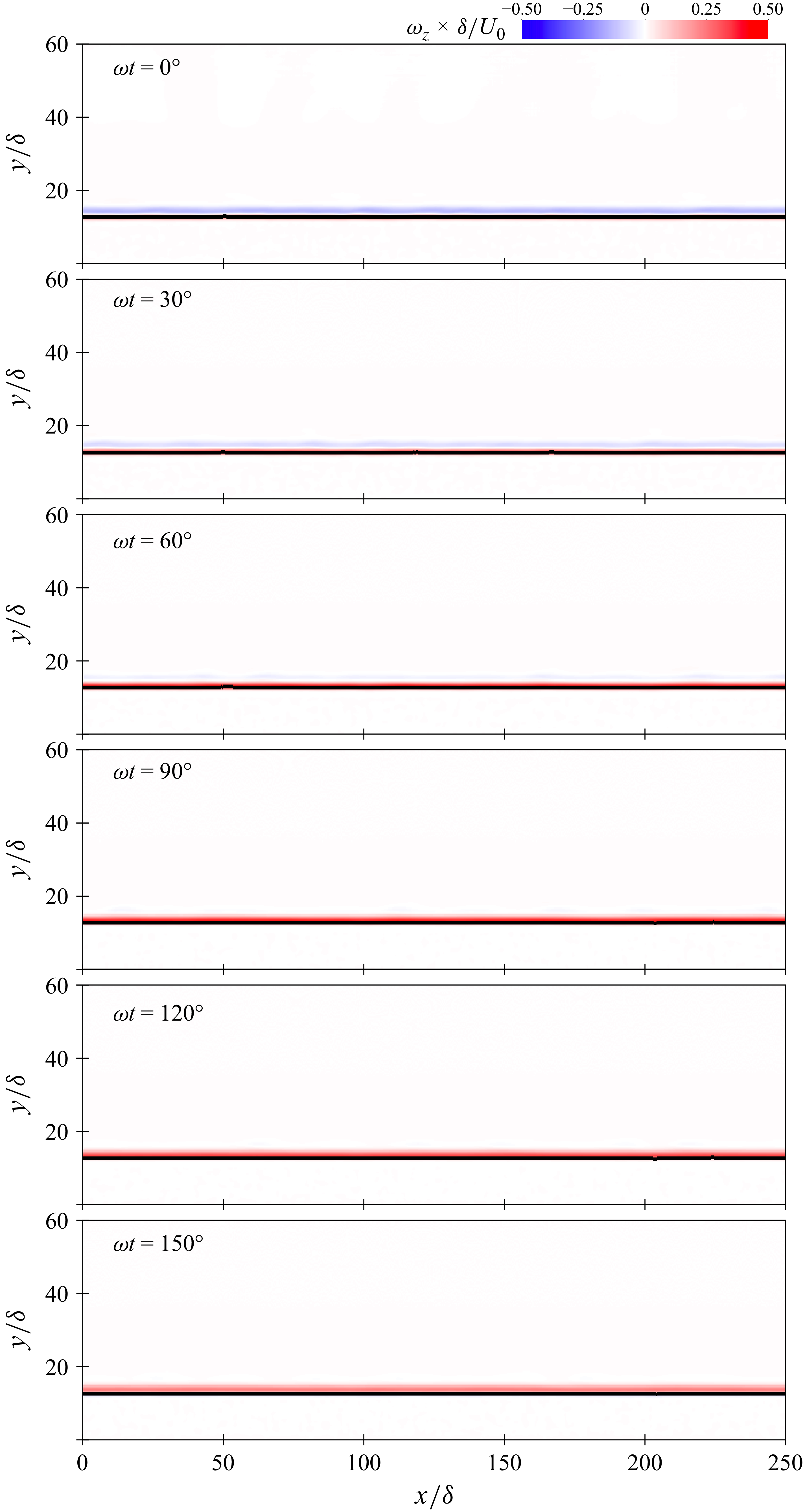
Figure 3. Zoomed-in views of the instantaneous spanwise vorticity and bed–fluid interface (solid line) at
 ${\textit{Re}}_{\delta }=200$
. Small ripples in the bedform cause flow disturbances and fluctuations associated with the disturbed laminar regime.
${\textit{Re}}_{\delta }=200$
. Small ripples in the bedform cause flow disturbances and fluctuations associated with the disturbed laminar regime.

Figure 4. Zoomed-in views of the instantaneous spanwise vorticity and bed–fluid interface (solid line) at
 ${\textit{Re}}_{\delta }=400$
. Increasing Reynolds number leads to greater flow disturbances and a dynamically evolving bed–fluid interface.
${\textit{Re}}_{\delta }=400$
. Increasing Reynolds number leads to greater flow disturbances and a dynamically evolving bed–fluid interface.
At
 ${\textit{Re}}_\delta =400$
, the particles in the bed’s top layers become mobile. This leads to a dynamically evolving bed–fluid interface and greater flow disturbances, as shown in figure 4. Flow disturbances are strongest around phases
${\textit{Re}}_\delta =400$
, the particles in the bed’s top layers become mobile. This leads to a dynamically evolving bed–fluid interface and greater flow disturbances, as shown in figure 4. Flow disturbances are strongest around phases
 $90^{\circ }$
and
$90^{\circ }$
and
 $120^{\circ }$
, i.e. from the maximum fluid velocity, and into the decelerating portion of the period. The vortex structures observed at these phases show chaotic behaviour, whereby larger structures spin off and break down into smaller ones. However, the range of scales is limited compared to what may be expected for a fully turbulent flow. The bed–fluid interface, marked by the black line in figure 4, changes dynamically with phase. This is due to particles being transported in the top layers of the bed, which couples the bedform dynamics to that of the flow over it.
$120^{\circ }$
, i.e. from the maximum fluid velocity, and into the decelerating portion of the period. The vortex structures observed at these phases show chaotic behaviour, whereby larger structures spin off and break down into smaller ones. However, the range of scales is limited compared to what may be expected for a fully turbulent flow. The bed–fluid interface, marked by the black line in figure 4, changes dynamically with phase. This is due to particles being transported in the top layers of the bed, which couples the bedform dynamics to that of the flow over it.
We also note that bed permeability is significant at
 ${\textit{Re}}_\delta =400$
. Whereas the extent of the flow intrusion below the bed–fluid interface is of the order of one Stokes thickness
${\textit{Re}}_\delta =400$
. Whereas the extent of the flow intrusion below the bed–fluid interface is of the order of one Stokes thickness
 $\delta$
at
$\delta$
at
 ${\textit{Re}}_\delta =200$
, the vortices generated at
${\textit{Re}}_\delta =200$
, the vortices generated at
 ${\textit{Re}}_\delta =400$
penetrate down by up to
${\textit{Re}}_\delta =400$
penetrate down by up to
 $4\delta$
, judging from figures 3 and 4. Owing to the bed permeability, these vortices push fluid into and out of the bed. This plays an important role in the dynamic evolution of the bed–fluid interface, as flow exiting the bed exerts an upward drag force on the particles that helps to suspend or set into motion particles in the bed’s top layers (Jewel, Fujisawa & Murakami Reference Jewel, Fujisawa and Murakami2019).
$4\delta$
, judging from figures 3 and 4. Owing to the bed permeability, these vortices push fluid into and out of the bed. This plays an important role in the dynamic evolution of the bed–fluid interface, as flow exiting the bed exerts an upward drag force on the particles that helps to suspend or set into motion particles in the bed’s top layers (Jewel, Fujisawa & Murakami Reference Jewel, Fujisawa and Murakami2019).
At
 ${\textit{Re}}_\delta = 800$
, figure 5 shows significant increase in flow disturbances over the bed, bed–fluid interface corrugations, and flow intrusion within the bed. The fluctuations’ intensity and spatial extent largely exceed those due to intermittent turbulence in the case of an OBL over a smooth and impermeable wall. The flow intrusion within the particle bed is also much greater at
${\textit{Re}}_\delta = 800$
, figure 5 shows significant increase in flow disturbances over the bed, bed–fluid interface corrugations, and flow intrusion within the bed. The fluctuations’ intensity and spatial extent largely exceed those due to intermittent turbulence in the case of an OBL over a smooth and impermeable wall. The flow intrusion within the particle bed is also much greater at
 ${\textit{Re}}_\delta =800$
compared to
${\textit{Re}}_\delta =800$
compared to
 ${\textit{Re}}_\delta =400$
. This likely contributes to the increased corrugation of the bed–fluid interface at this Reynolds number. Further, the bed–fluid interface is most corrugated around phases
${\textit{Re}}_\delta =400$
. This likely contributes to the increased corrugation of the bed–fluid interface at this Reynolds number. Further, the bed–fluid interface is most corrugated around phases
 $60^{\circ }$
,
$60^{\circ }$
,
 $90^{\circ }$
and
$90^{\circ }$
and
 $120^{\circ }$
, which correspond to the phases with largest flow intrusion.
$120^{\circ }$
, which correspond to the phases with largest flow intrusion.
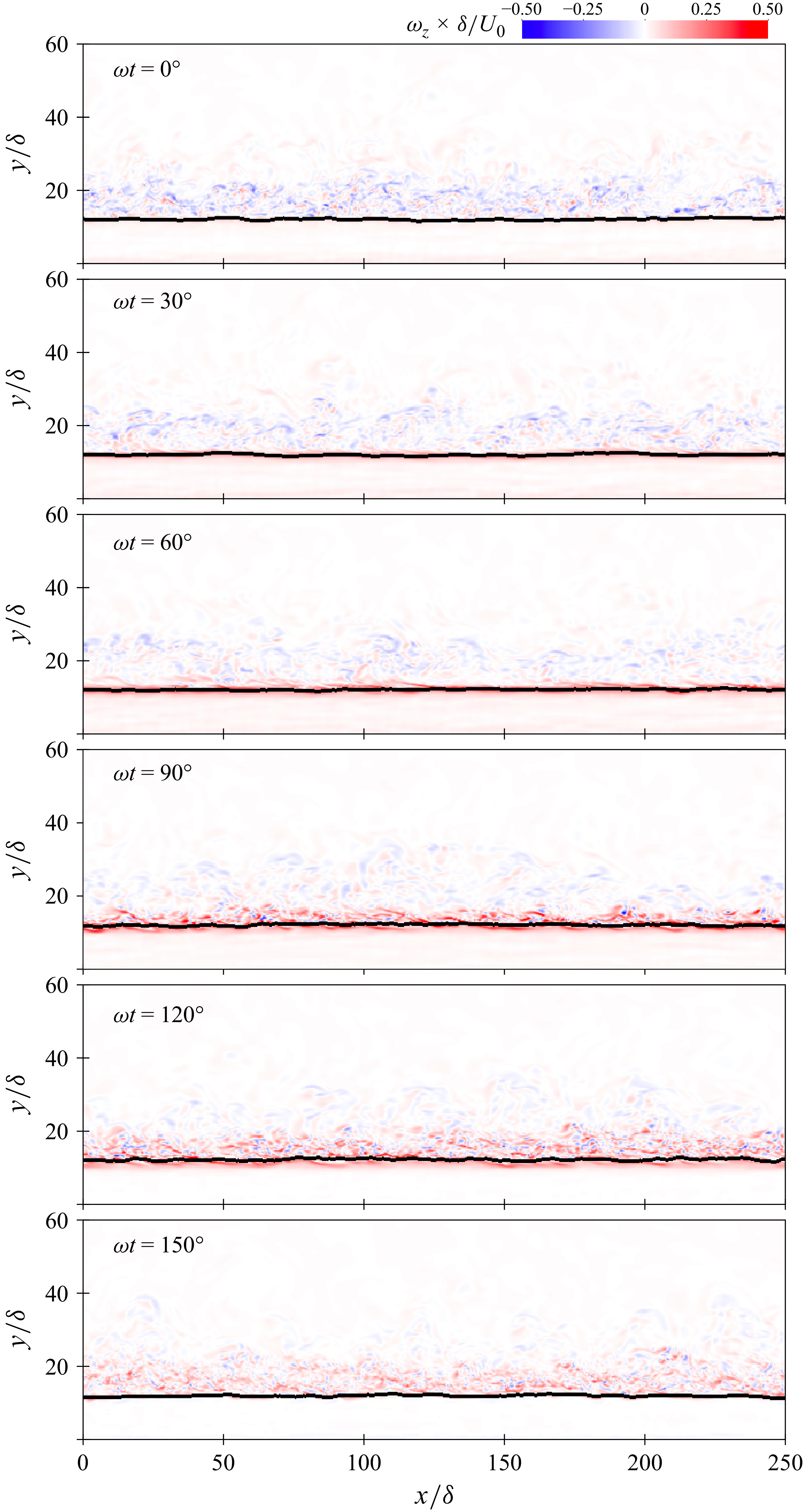
Figure 5. Zoomed-in views of the instantaneous spanwise vorticity and bed–fluid interface (solid line) at
 ${\textit{Re}}_{\delta }=800$
. The bedform shifts into ripples at various phases. The shedding vortices create a large range of scales. The eddies penetrate the bed interface.
${\textit{Re}}_{\delta }=800$
. The bedform shifts into ripples at various phases. The shedding vortices create a large range of scales. The eddies penetrate the bed interface.
4.2. Fluid statistics
Having established the qualitative dynamics of these flows in § 4.1, we now characterise the fluid phase with quantitative measures.
Figures 6(a), 6(c) and 6(e) show vertical profiles of phase-averaged mean streamwise fluid velocity
 $\langle u_{\!f}\rangle _{xz}$
from the cases with particle bed at
$\langle u_{\!f}\rangle _{xz}$
from the cases with particle bed at
 ${\textit{Re}}_\delta =200$
, 400 and 800. To better appreciate the change caused by the particle bed, we also report data from the companion runs with a bottom smooth and impermeable wall discussed in Appendix A. In this figure,
${\textit{Re}}_\delta =200$
, 400 and 800. To better appreciate the change caused by the particle bed, we also report data from the companion runs with a bottom smooth and impermeable wall discussed in Appendix A. In this figure,
 $y_b$
denotes the average bed height. We determine the latter by computing the average
$y_b$
denotes the average bed height. We determine the latter by computing the average
 $y$
location of the isovolume
$y$
location of the isovolume
 $\alpha =\alpha _b=0.2$
, which represents the bed–fluid interface.
$\alpha =\alpha _b=0.2$
, which represents the bed–fluid interface.

Figure 6. Statistics of the phase-averaged mean streamwise velocity at (a,b)
 ${\textit{Re}}_\delta =200$
, (c,d)
${\textit{Re}}_\delta =200$
, (c,d)
 ${\textit{Re}}_\delta =400$
, and (e,f)
${\textit{Re}}_\delta =400$
, and (e,f)
 ${\textit{Re}}_\delta =800$
. The lines correspond to phases
${\textit{Re}}_\delta =800$
. The lines correspond to phases
 $\omega t =0^\circ$
(
$\omega t =0^\circ$
(
![]() ),
),
 $\omega t =30^\circ$
(
$\omega t =30^\circ$
(
![]() ),
),
 $\omega t =60^\circ$
(
$\omega t =60^\circ$
(
![]() ),
),
 $\omega t =90^\circ$
(
$\omega t =90^\circ$
(
![]() ),
),
 $\omega t =120^\circ$
(
$\omega t =120^\circ$
(
![]() ), and
), and
 $\omega t =150^\circ$
(
$\omega t =150^\circ$
(
![]() ). The dashed lines correspond to the smooth wall simulations from Appendix A.
). The dashed lines correspond to the smooth wall simulations from Appendix A.
At
 ${\textit{Re}}_\delta =200$
, the average streamwise fluid velocity from the cases with a particle bed and smooth impermeable wall are sensibly close and follow the laminar Stokes solution. The notable differences include a marginally thicker boundary layer, a significant slip velocity
${\textit{Re}}_\delta =200$
, the average streamwise fluid velocity from the cases with a particle bed and smooth impermeable wall are sensibly close and follow the laminar Stokes solution. The notable differences include a marginally thicker boundary layer, a significant slip velocity
 $u_{f,I}$
at the bed–fluid interface
$u_{f,I}$
at the bed–fluid interface
 $y=y_b$
, which reaches up to
$y=y_b$
, which reaches up to
 $u_{f,I}\simeq 0.1\,U_0$
at phase
$u_{f,I}\simeq 0.1\,U_0$
at phase
 $60^\circ$
, and interstitial flow that decays quickly within
$60^\circ$
, and interstitial flow that decays quickly within
 $1.5\delta$
of depth. These features are characteristic of permeable interfaces (Voermans et al. Reference Voermans, Ghisalberti and Ivey2017), although their net effect on the average streamwise fluid velocity profiles at
$1.5\delta$
of depth. These features are characteristic of permeable interfaces (Voermans et al. Reference Voermans, Ghisalberti and Ivey2017), although their net effect on the average streamwise fluid velocity profiles at
 ${\textit{Re}}_\delta =200$
is limited.
${\textit{Re}}_\delta =200$
is limited.
With increasing
 ${\textit{Re}}_\delta$
, the differences between cases with particle bed and cases with a smooth and impermeable wall accentuate as effects due to bed permeability effects increase. Most notably, we note the increase of the boundary layer thickness, interfacial slip velocity, and depth of the interstitial flow. At
${\textit{Re}}_\delta$
, the differences between cases with particle bed and cases with a smooth and impermeable wall accentuate as effects due to bed permeability effects increase. Most notably, we note the increase of the boundary layer thickness, interfacial slip velocity, and depth of the interstitial flow. At
 ${\textit{Re}}_\delta =400$
, the interfacial slip velocity peaks at
${\textit{Re}}_\delta =400$
, the interfacial slip velocity peaks at
 $u_{f,I}\simeq 0.17\,U_0$
at phase
$u_{f,I}\simeq 0.17\,U_0$
at phase
 $60^\circ$
, while the flow extends below the bed–fluid interface by up to
$60^\circ$
, while the flow extends below the bed–fluid interface by up to
 $9\delta$
. At
$9\delta$
. At
 ${\textit{Re}}_\delta =800$
, the maximum slip velocity increases to
${\textit{Re}}_\delta =800$
, the maximum slip velocity increases to
 $u_{f,I}\simeq 0.52\, U_0$
, and the flow extends below the bed–fluid interface by up to
$u_{f,I}\simeq 0.52\, U_0$
, and the flow extends below the bed–fluid interface by up to
 $14\, \delta$
.
$14\, \delta$
.
In addition to altering the mean velocity profiles, the presence of a particle bed leads to greater velocity fluctuations than in the smooth wall cases. Figures 6(b), 6(d) and 6(f) show the streamwise velocity fluctuations for each Reynolds number. While the root mean square (rms) of the streamwise velocity fluctuations
 $u_{f,rms}$
in cases with a smooth and impermeable wall at
$u_{f,rms}$
in cases with a smooth and impermeable wall at
 ${\textit{Re}}_\delta = 200$
and 400 are identically zero, we note the existence of significant fluctuations in the cases with particle bed and at matching Reynolds numbers. For
${\textit{Re}}_\delta = 200$
and 400 are identically zero, we note the existence of significant fluctuations in the cases with particle bed and at matching Reynolds numbers. For
 ${\textit{Re}}_\delta = 200$
,
${\textit{Re}}_\delta = 200$
,
 $u_{f,rms}$
peaks at approximately 13 % of the velocity amplitude and approximately
$u_{f,rms}$
peaks at approximately 13 % of the velocity amplitude and approximately
 $1.4\delta$
above the bed. At
$1.4\delta$
above the bed. At
 ${\textit{Re}}_\delta = 400$
,
${\textit{Re}}_\delta = 400$
,
 $u_{f,rms}$
peaks at 13 % of the velocity amplitude
$u_{f,rms}$
peaks at 13 % of the velocity amplitude
 $U_0$
at phase
$U_0$
at phase
 $90^\circ$
and approximately
$90^\circ$
and approximately
 $1.5 \delta$
above the bed. At
$1.5 \delta$
above the bed. At
 ${\textit{Re}}_\delta = 800$
, the
${\textit{Re}}_\delta = 800$
, the
 $u_{f,rms}$
profiles are widest, indicating that the flow disturbances extend to approximately
$u_{f,rms}$
profiles are widest, indicating that the flow disturbances extend to approximately
 $20\delta$
–
$20\delta$
–
 $30\delta$
above the bed. The highest fluctuations occur at phase
$30\delta$
above the bed. The highest fluctuations occur at phase
 $90^\circ$
and reach approximately 6.9 % of the velocity amplitude. It is important to note that at
$90^\circ$
and reach approximately 6.9 % of the velocity amplitude. It is important to note that at
 ${\textit{Re}}_\delta = 400$
and
${\textit{Re}}_\delta = 400$
and
 $800$
, velocity fluctuations are no longer homogeneous in the streamwise direction due to the waviness of the bed–fluid interface. For
$800$
, velocity fluctuations are no longer homogeneous in the streamwise direction due to the waviness of the bed–fluid interface. For
 ${\textit{Re}}_\delta = 400$
and
${\textit{Re}}_\delta = 400$
and
 $800$
, the velocity fluctuations drop to below 0.1 % of the velocity amplitude (
$800$
, the velocity fluctuations drop to below 0.1 % of the velocity amplitude (
 $U_0$
) at
$U_0$
) at
 $60\delta$
from the bed–fluid interface.
$60\delta$
from the bed–fluid interface.
The particle bed leads to a different condition at the bed–fluid interface as compared to a smooth wall. In the smooth wall case, no-slip applies at the wall, while the particle bed is porous, which leads to a slip velocity at the bed–fluid interface. This causes the bed shear stress to drop compared to the smooth wall case. Predicting the sediment transport is dependent upon accurate values of the bed shear stress, or non-dimensionally, the Shields number
 $\theta$
. The Shields number can be estimated a priori using the single-phase wall shear stress, i.e.
$\theta$
. The Shields number can be estimated a priori using the single-phase wall shear stress, i.e.
 $\tau _w=\mu\, \left .({\partial u}/{\partial y})\right |_{y=0}$
. We denote this Shields number as
$\tau _w=\mu\, \left .({\partial u}/{\partial y})\right |_{y=0}$
. We denote this Shields number as
 $\theta _{{wall}}=\tau _w/((\rho _{\!p}-\rho _{\!f})g d_{\!p})$
. Alternatively, the bed shear stress can be defined using the shear stress conditioned on an isosurface corresponding to the bed–fluid interface
$\theta _{{wall}}=\tau _w/((\rho _{\!p}-\rho _{\!f})g d_{\!p})$
. Alternatively, the bed shear stress can be defined using the shear stress conditioned on an isosurface corresponding to the bed–fluid interface
 $\alpha _{\!p} = \alpha _{p,b}$
(Arolla & Desjardins Reference Arolla and Desjardins2015). We evaluate this in two ways. The first way follows the calculation of Arolla & Desjardins (Reference Arolla and Desjardins2015), i.e.
$\alpha _{\!p} = \alpha _{p,b}$
(Arolla & Desjardins Reference Arolla and Desjardins2015). We evaluate this in two ways. The first way follows the calculation of Arolla & Desjardins (Reference Arolla and Desjardins2015), i.e.
 \begin{equation} \tau _b = (\mu +\mu ^\star ) \left . \left\langle \frac {\overline {\partial u}}{\partial y} \right\rangle \right |_{y_b}=\mu \alpha ^{-2.8} \left . \left\langle \frac {\overline {\partial u}}{\partial y} \right\rangle \right |_{y_b}. \end{equation}
We denote the Shields number based on the expression above as
 $\theta _{{bed}}^{(1)}$
. Note that this evaluation does not account for the waviness of the bedform. To deal with this, we carry out an alternative computation of the bed shear stress by interpolating the deviatoric stress tensor to the bed–fluid interface. Figure 7 shows an example of instantaneous isosurface
$\theta _{{bed}}^{(1)}$
. Note that this evaluation does not account for the waviness of the bedform. To deal with this, we carry out an alternative computation of the bed shear stress by interpolating the deviatoric stress tensor to the bed–fluid interface. Figure 7 shows an example of instantaneous isosurface
 $\alpha =\alpha _b$
representing the bed–fluid interface. In this second approach, we determine the bed shear
$\alpha =\alpha _b$
representing the bed–fluid interface. In this second approach, we determine the bed shear
 $\tau _b$
using
$\tau _b$
using
 \begin{equation} \tau _b = \left \|\frac {1}{A_I}\iint _{S_I} \boldsymbol{n}\boldsymbol{\cdot }\boldsymbol{\tau '}\,{\rm d}S\right \|, \end{equation}
where
 $S_I$
represents the bed–fluid interface,
$S_I$
represents the bed–fluid interface,
 $A_I$
is the total interfacial area,
$A_I$
is the total interfacial area,
 $\boldsymbol{n}$
is the normal vector on the isosurface
$\boldsymbol{n}$
is the normal vector on the isosurface
 $\alpha _{\!p}=\alpha _{p,b}$
, and
$\alpha _{\!p}=\alpha _{p,b}$
, and
 $\boldsymbol{\tau}'=\mu [\boldsymbol{\nabla }\boldsymbol{u} +\boldsymbol{\nabla }\boldsymbol{u}^{\rm T}- (2/3)(\boldsymbol{\nabla }\boldsymbol{\cdot }\boldsymbol{u})\boldsymbol{I}]+\boldsymbol{R}_\mu $
is the deviatoric stress tensor. With the closure of Gibilaro et al. (Reference Gibilaro, Gallucci, Di Felice and Pagliai2007), this tensor reads
$\boldsymbol{\tau}'=\mu [\boldsymbol{\nabla }\boldsymbol{u} +\boldsymbol{\nabla }\boldsymbol{u}^{\rm T}- (2/3)(\boldsymbol{\nabla }\boldsymbol{\cdot }\boldsymbol{u})\boldsymbol{I}]+\boldsymbol{R}_\mu $
is the deviatoric stress tensor. With the closure of Gibilaro et al. (Reference Gibilaro, Gallucci, Di Felice and Pagliai2007), this tensor reads
 \begin{equation} \boldsymbol{\tau}'=\mu \alpha _{\!f}^{-2.8} \left (\boldsymbol{\nabla }\boldsymbol{u} +\boldsymbol{\nabla }\boldsymbol{u}^{\rm T}- (2/3)(\boldsymbol{\nabla }\boldsymbol{\cdot }\boldsymbol{u})\boldsymbol{I}\right ). \end{equation}
We denote the resulting Shields number as
 $\theta _{{bed}}^{(2)}$
.
$\theta _{{bed}}^{(2)}$
.

Figure 7. The
 ${\textit{Re}}_\delta = 400$
bedform height deviations. Small ripples rise and fall below the average bed height.
${\textit{Re}}_\delta = 400$
bedform height deviations. Small ripples rise and fall below the average bed height.
Figure 8 shows the evolution of
 $\theta _{{wall}}$
,
$\theta _{{wall}}$
,
 $\theta _{{bed}}^{(1)}$
and
$\theta _{{bed}}^{(1)}$
and
 $\theta _{{bed}}^{(2)}$
during a full cycle. We also report the maximum Shields number obtained with each method in table 3. We note close agreement between
$\theta _{{bed}}^{(2)}$
during a full cycle. We also report the maximum Shields number obtained with each method in table 3. We note close agreement between
 $\theta _{{bed}}^{(1)}$
and
$\theta _{{bed}}^{(1)}$
and
 $\theta _{{bed}}^{(2)}$
at all Reynolds numbers. This indicates that the bed waviness does not have a significant effect on the bed shear stress in these cases. Regardless of the method used, the Shields number estimated using the bed shear stress (
$\theta _{{bed}}^{(2)}$
at all Reynolds numbers. This indicates that the bed waviness does not have a significant effect on the bed shear stress in these cases. Regardless of the method used, the Shields number estimated using the bed shear stress (
 $\theta _{{bed}}^{(1)}$
and
$\theta _{{bed}}^{(1)}$
and
 $\theta _{{bed}}^{(2)}$
) is much lower than the Shields number based on single-phase wall shear stress
$\theta _{{bed}}^{(2)}$
) is much lower than the Shields number based on single-phase wall shear stress
 $\theta _{{wall}}$
, even at
$\theta _{{wall}}$
, even at
 ${\textit{Re}}_\delta =200$
. This was also noted by Kidanemariam & Uhlmann (Reference Kidanemariam and Uhlmann2014) in PR-DNS of laminar channel flow with a sediment bed. They observed a progressive departure of the Shields number from the Poiseuille predictions with increasing fluid flow rate, caused by the departure of the flow profile from a strictly parabolic profile at the bed interface. Likewise, flow intrusion through the sediment bed leads to lower gradients at the bed as shown in figure 6, which in turn leads to lower bed shear stress.
${\textit{Re}}_\delta =200$
. This was also noted by Kidanemariam & Uhlmann (Reference Kidanemariam and Uhlmann2014) in PR-DNS of laminar channel flow with a sediment bed. They observed a progressive departure of the Shields number from the Poiseuille predictions with increasing fluid flow rate, caused by the departure of the flow profile from a strictly parabolic profile at the bed interface. Likewise, flow intrusion through the sediment bed leads to lower gradients at the bed as shown in figure 6, which in turn leads to lower bed shear stress.

Figure 8. Variation of the Shields number with the phase: squares indicate
 $\theta _{{wall}}$
; pentagons indicate
$\theta _{{wall}}$
; pentagons indicate
 $\theta _{{bed}}^{(1)}$
; diamonds indicate
$\theta _{{bed}}^{(1)}$
; diamonds indicate
 $\theta _{{bed}}^{(2)}$
. (a)
$\theta _{{bed}}^{(2)}$
. (a)
 ${\textit{Re}}_\delta = 200$
, (b)
${\textit{Re}}_\delta = 200$
, (b)
 ${\textit{Re}}_\delta = 400$
and (c)
${\textit{Re}}_\delta = 400$
and (c)
 ${\textit{Re}}_\delta = 800$
.
${\textit{Re}}_\delta = 800$
.
Table 3. Maximum values of the Shields number by method of computation.

4.3. Particle statistics
Next, we analyse the characteristics of the particulate phase and how these relate to those of the fluid phase.
At
 ${\textit{Re}}_\delta =400$
, the particle bed is characterised by the periodic particle transport at the ripple crests. This can be seen in figure 9(a), which depicts a top-down view of the particle bed between
${\textit{Re}}_\delta =400$
, the particle bed is characterised by the periodic particle transport at the ripple crests. This can be seen in figure 9(a), which depicts a top-down view of the particle bed between
 $\omega t=0^\circ$
and
$\omega t=0^\circ$
and
 $\omega t=150^\circ$
, and where the particles are coloured by their normalised streamwise velocities. At phase
$\omega t=150^\circ$
, and where the particles are coloured by their normalised streamwise velocities. At phase
 $0^\circ$
, most particles are immobile and within the bed. From there, the rising fluid velocity initiates particle saltation at the ripple crests, which are well visible at phase
$0^\circ$
, most particles are immobile and within the bed. From there, the rising fluid velocity initiates particle saltation at the ripple crests, which are well visible at phase
 $60^\circ$
. These ripples are quasi-two-dimensional and display wavelength approximately
$60^\circ$
. These ripples are quasi-two-dimensional and display wavelength approximately
 $\sim 60\delta$
. The rolling ripples continue intensifying until phase
$\sim 60\delta$
. The rolling ripples continue intensifying until phase
 $90^\circ$
. After that, the decrease in fluid velocity leads to a slow down of the particles until all are immobile again by phase
$90^\circ$
. After that, the decrease in fluid velocity leads to a slow down of the particles until all are immobile again by phase
 $150^\circ$
. This process occurs again, albeit in the reverse direction, between phases
$150^\circ$
. This process occurs again, albeit in the reverse direction, between phases
 $180^\circ$
and
$180^\circ$
and
 $360^\circ$
.
$360^\circ$
.

Figure 9. Top-down views of the particle bed at phases
 $0^\circ$
,
$0^\circ$
,
 $30^\circ$
,
$30^\circ$
,
 $60^\circ$
,
$60^\circ$
,
 $90^\circ$
,
$90^\circ$
,
 $120^\circ$
,
$120^\circ$
,
 $150^\circ$
for (a)
$150^\circ$
for (a)
 ${\textit{Re}}_\delta = 400$
and (b)
${\textit{Re}}_\delta = 400$
and (b)
 ${\textit{Re}}_\delta = 800$
. The particles are coloured by their normalised streamwise velocity. The case at
${\textit{Re}}_\delta = 800$
. The particles are coloured by their normalised streamwise velocity. The case at
 ${\textit{Re}}_\delta =400$
shows periodic rolling ripples, whereas the case at
${\textit{Re}}_\delta =400$
shows periodic rolling ripples, whereas the case at
 ${\textit{Re}}_\delta =800$
exhibits a particle suspension layer, and may be evolving towards a new bedform.
${\textit{Re}}_\delta =800$
exhibits a particle suspension layer, and may be evolving towards a new bedform.
With increasing
 ${\textit{Re}}_\delta$
to 800, the bed may be evolving towards a new bedform with wavelength greater than
${\textit{Re}}_\delta$
to 800, the bed may be evolving towards a new bedform with wavelength greater than
 $L_x$
. As shown in figure 9(b), the rolling ripples noted at
$L_x$
. As shown in figure 9(b), the rolling ripples noted at
 ${\textit{Re}}_\delta =400$
are no longer present at
${\textit{Re}}_\delta =400$
are no longer present at
 ${\textit{Re}}_\delta =800$
. Instead, we note the periodic emergence and collapse of a layer of suspended particles over the bed. At phase
${\textit{Re}}_\delta =800$
. Instead, we note the periodic emergence and collapse of a layer of suspended particles over the bed. At phase
 $0^\circ$
, most particles start at rest in the bed. As the flow accelerates, particles in the top layer of the bed start saltating, which can be seen at phase
$0^\circ$
, most particles start at rest in the bed. As the flow accelerates, particles in the top layer of the bed start saltating, which can be seen at phase
 $30^{\circ }$
. As the fluid velocity continues increasing, more particles are set in motion. At phase
$30^{\circ }$
. As the fluid velocity continues increasing, more particles are set in motion. At phase
 $60^\circ$
, we note that a large number of particles are suspended within the fluid column. The layer of suspended particles continues growing up to phase
$60^\circ$
, we note that a large number of particles are suspended within the fluid column. The layer of suspended particles continues growing up to phase
 $120^{\circ }$
, by which point the fluid velocity has begun decreasing. With the continued slowing down of the flow, most particles redeposit in the bed by phase
$120^{\circ }$
, by which point the fluid velocity has begun decreasing. With the continued slowing down of the flow, most particles redeposit in the bed by phase
 $150^\circ$
, while only few remain suspended.
$150^\circ$
, while only few remain suspended.
Note that we do not present figures similar to figures 9(a) and 9(b) for the case at
 ${\textit{Re}}_\delta =200$
because particle motion is negligible in that case.
${\textit{Re}}_\delta =200$
because particle motion is negligible in that case.
Figure 10 shows the bed surface interface averaged over the spanwise direction, for
 ${\textit{Re}}_\delta = 400$
and 800. The different lines correspond to the interface locations from periods 2–10. At
${\textit{Re}}_\delta = 400$
and 800. The different lines correspond to the interface locations from periods 2–10. At
 ${\textit{Re}}_\delta = 400$
, the bed–fluid interface in figure 10(a) develops into a clear bedform as the simulation progress. The wavelength associated with the ripples is
${\textit{Re}}_\delta = 400$
, the bed–fluid interface in figure 10(a) develops into a clear bedform as the simulation progress. The wavelength associated with the ripples is
 $\lambda /\delta = 62.6$
. The typical height of the ripples, measured from depression to peak, is approximately
$\lambda /\delta = 62.6$
. The typical height of the ripples, measured from depression to peak, is approximately
 $4\delta$
at phase
$4\delta$
at phase
 $90^\circ$
. While sediment particles move along the bed at significant velocities, as seen from figure 9(a), the bedform evolves on a much slower periodic time scale. At
$90^\circ$
. While sediment particles move along the bed at significant velocities, as seen from figure 9(a), the bedform evolves on a much slower periodic time scale. At
 ${\textit{Re}}_\delta = 800$
, the bed surface displays a range of small-scale corrugations. However, the large-scale ripples disappear. Figure 10(b) shows that the bed height deviations drop below
${\textit{Re}}_\delta = 800$
, the bed surface displays a range of small-scale corrugations. However, the large-scale ripples disappear. Figure 10(b) shows that the bed height deviations drop below
 $2\delta$
. This is because particle transport takes place primarily in a suspension layer.
$2\delta$
. This is because particle transport takes place primarily in a suspension layer.

Figure 10. Bed interfaces for (a)
 ${\textit{Re}}_\delta = 400$
and (b)
${\textit{Re}}_\delta = 400$
and (b)
 ${\textit{Re}}_\delta = 800$
. Darker lines indicate later periods. For
${\textit{Re}}_\delta = 800$
. Darker lines indicate later periods. For
 ${\textit{Re}}_\delta = 400$
, rolling-grain ripples emerge and move through the domain, but the dominant wavelength does not change. At
${\textit{Re}}_\delta = 400$
, rolling-grain ripples emerge and move through the domain, but the dominant wavelength does not change. At
 ${\textit{Re}}_\delta = 800$
, the bed height becomes highly corrugated, and the bed–fluid interface breaks down.
${\textit{Re}}_\delta = 800$
, the bed height becomes highly corrugated, and the bed–fluid interface breaks down.
Next, we report the vertical profiles of normalised particle velocity in figures 11(a) and 11(b). At
 ${\textit{Re}}_\delta =400$
, the normalised particle velocity is small, as
${\textit{Re}}_\delta =400$
, the normalised particle velocity is small, as
 $\langle \alpha _{\!p} u_{\!p}\rangle _{xz}/U_0\lt 0.025$
for all phases. This indicates that the rolling ripples move at a velocity much smaller than the fluid velocity amplitude
$\langle \alpha _{\!p} u_{\!p}\rangle _{xz}/U_0\lt 0.025$
for all phases. This indicates that the rolling ripples move at a velocity much smaller than the fluid velocity amplitude
 $U_0$
. The largest particle velocity occurs at phase
$U_0$
. The largest particle velocity occurs at phase
 $30^\circ$
, in agreement with the qualitative observations from figure 9(a). We note that the particle velocity is non-zero only in a region of width
$30^\circ$
, in agreement with the qualitative observations from figure 9(a). We note that the particle velocity is non-zero only in a region of width
 $\sim 8\delta$
around the average bed height
$\sim 8\delta$
around the average bed height
 $y_b$
. The width of this region is controlled by the height of the ripples, noted in figure 10(a), and is not due to suspended particles, as the latter are negligible at
$y_b$
. The width of this region is controlled by the height of the ripples, noted in figure 10(a), and is not due to suspended particles, as the latter are negligible at
 ${\textit{Re}}_\delta =400$
. In contrast, the normalised particle velocity reaches significantly higher values and displays wider distribution at
${\textit{Re}}_\delta =400$
. In contrast, the normalised particle velocity reaches significantly higher values and displays wider distribution at
 ${\textit{Re}}_\delta =800$
. At phase
${\textit{Re}}_\delta =800$
. At phase
 $150^\circ$
, the region of non-zero particle momentum is approximately
$150^\circ$
, the region of non-zero particle momentum is approximately
 $18\delta$
thick and peaks at approximately
$18\delta$
thick and peaks at approximately
 $0.08\rho _{\!p} U_0$
. The widening of the profile and the absence of large-scale deformations of the bed–fluid interface indicate that the amount of suspended particles is significantly larger at
$0.08\rho _{\!p} U_0$
. The widening of the profile and the absence of large-scale deformations of the bed–fluid interface indicate that the amount of suspended particles is significantly larger at
 ${\textit{Re}}_\delta =800$
compared to
${\textit{Re}}_\delta =800$
compared to
 ${\textit{Re}}_\delta =400$
. This is also in agreement with the qualitative observations from figure 9(b).
${\textit{Re}}_\delta =400$
. This is also in agreement with the qualitative observations from figure 9(b).

Figure 11. Normalised particle momentum profiles and mass fluxes at (a,c)
 ${\textit{Re}}_\delta =400$
and (b,d)
${\textit{Re}}_\delta =400$
and (b,d)
 ${\textit{Re}}_\delta =800$
. The lines in (a,b) correspond to phases
${\textit{Re}}_\delta =800$
. The lines in (a,b) correspond to phases
 $\omega t =0^\circ$
(
$\omega t =0^\circ$
(
![]() ),
),
 $\omega t =30^\circ$
(
$\omega t =30^\circ$
(
![]() ),
),
 $\omega t =60^\circ$
(
$\omega t =60^\circ$
(
![]() ),
),
 $\omega t =90^\circ$
(
$\omega t =90^\circ$
(
![]() ),
),
 $\omega t =120^\circ$
(
$\omega t =120^\circ$
(
![]() ), and
), and
 $\omega t =150^\circ$
(
$\omega t =150^\circ$
(
![]() ). Significant particle momentum is seen near the bed interface, indicating particle motion at approximately the bed interface.
). Significant particle momentum is seen near the bed interface, indicating particle motion at approximately the bed interface.
With regards to the computational aspects, we note that the particle velocity is negligible at approximately
 $\sim 10\delta$
below the bed–fluid interface
$\sim 10\delta$
below the bed–fluid interface
 $y_b$
at all phases and
$y_b$
at all phases and
 ${\textit{Re}}_\delta$
considered. This shows that the particle bed in our simulations, which has initial height
${\textit{Re}}_\delta$
considered. This shows that the particle bed in our simulations, which has initial height
 $H_b=16.7\delta$
, is sufficiently tall to capture the dynamics near the bed–fluid interface without interference from boundary conditions at the bottom of the domain.
$H_b=16.7\delta$
, is sufficiently tall to capture the dynamics near the bed–fluid interface without interference from boundary conditions at the bottom of the domain.
Figures 11(c) and 11(d) show the evolution of the normalised sediment flow rate
 $q_s$
over a half-period, for
$q_s$
over a half-period, for
 ${\textit{Re}}_\delta = 400$
and
${\textit{Re}}_\delta = 400$
and
 $800$
. We compute
$800$
. We compute
 $q_s$
by integrating the particle velocity profiles over the vertical direction, i.e.
$q_s$
by integrating the particle velocity profiles over the vertical direction, i.e.
 \begin{equation} q_s = \int _{0}^{L_y} \langle \alpha _{\!p} u_{\!p} \rangle _{xz}\, {\rm d}y. \end{equation}
At
 ${\textit{Re}}_\delta = 400$
, the sediment volumetric flux peaks at
${\textit{Re}}_\delta = 400$
, the sediment volumetric flux peaks at
 $1.76$
at phase
$1.76$
at phase
 $\omega t = 30^\circ$
. Notably, the sediment transport is not symmetric for the accelerating and decelerating portions of the periods. At
$\omega t = 30^\circ$
. Notably, the sediment transport is not symmetric for the accelerating and decelerating portions of the periods. At
 ${\textit{Re}}_\delta = 800$
, the sediment flux is more than 12 times greater than at
${\textit{Re}}_\delta = 800$
, the sediment flux is more than 12 times greater than at
 ${\textit{Re}}_\delta =400$
. The maximum normalised flux is
${\textit{Re}}_\delta =400$
. The maximum normalised flux is
 $25.8$
at phase
$25.8$
at phase
 $60^\circ$
. Here, too, we note an asymmetry between the acceleration and deceleration portions of the period.
$60^\circ$
. Here, too, we note an asymmetry between the acceleration and deceleration portions of the period.
5. Discussion and conclusions
In this study, we analyse data obtained from Euler–Lagrange simulations of an oscillatory boundary layer (OBL) developing over a bed of collisional and freely moving sediment grains with density ratio
 $\rho _{\!p}/\rho _{\!f}=2.65$
and Galileo number
$\rho _{\!p}/\rho _{\!f}=2.65$
and Galileo number
 ${\textit{Ga}}=51.9$
. In these simulations, we vary the velocity amplitude to yield Reynolds numbers
${\textit{Ga}}=51.9$
. In these simulations, we vary the velocity amplitude to yield Reynolds numbers
 ${\textit{Re}}_\delta =200{-}800$
. The maximum Shields number based on the smooth wall case also varies from
${\textit{Re}}_\delta =200{-}800$
. The maximum Shields number based on the smooth wall case also varies from
 $5.60\times10^{-2}$
to
$5.60\times10^{-2}$
to
 $2.43\times10^{-1}$
, and the Keulegan–Carpenter number varies from
$2.43\times10^{-1}$
, and the Keulegan–Carpenter number varies from
 $134.5$
to
$134.5$
to
 $538.0$
. Companion simulations of an OBL over a smooth and impermeable wall show that the boundary layer follows the laminar Stokes solution at
$538.0$
. Companion simulations of an OBL over a smooth and impermeable wall show that the boundary layer follows the laminar Stokes solution at
 ${\textit{Re}}_\delta =200$
and
${\textit{Re}}_\delta =200$
and
 ${\textit{Re}}_\delta =400$
, and displays intermittent turbulence at
${\textit{Re}}_\delta =400$
, and displays intermittent turbulence at
 ${\textit{Re}}_\delta =800$
. However, the presence of a mobile bed alters the flow characteristics and leads to a coupling of the dynamics of the OBL with that of the sediment bed.
${\textit{Re}}_\delta =800$
. However, the presence of a mobile bed alters the flow characteristics and leads to a coupling of the dynamics of the OBL with that of the sediment bed.
The coupled dynamics arise from two fundamental mechanisms. The first one relates to the bed permeability. This is due to the porosity of the bed, which allows the flow to penetrate within the sediment layers. The extent of the flow penetration depends on the Reynolds number. In the case
 ${\textit{Re}}_\delta =200$
, the flow penetration is of the order of the Stokes thickness
${\textit{Re}}_\delta =200$
, the flow penetration is of the order of the Stokes thickness
 $\delta$
. With increasing
$\delta$
. With increasing
 ${\textit{Re}}_\delta$
, the flow penetration increases to approximately
${\textit{Re}}_\delta$
, the flow penetration increases to approximately
 $9\delta$
and
$9\delta$
and
 $14\delta$
at
$14\delta$
at
 ${\textit{Re}}_\delta =400$
and
${\textit{Re}}_\delta =400$
and
 ${\textit{Re}}_\delta =800$
, respectively. Another consequence of the bed permeability is the emergence of a slip velocity at the bed–fluid interface. At phase
${\textit{Re}}_\delta =800$
, respectively. Another consequence of the bed permeability is the emergence of a slip velocity at the bed–fluid interface. At phase
 $30^\circ$
of the cycle, the interfacial slip velocity peaks at approximately
$30^\circ$
of the cycle, the interfacial slip velocity peaks at approximately
 $0.12U_0$
at
$0.12U_0$
at
 ${\textit{Re}}_\delta =200$
,
${\textit{Re}}_\delta =200$
,
 $0.17U_0$
at phase
$0.17U_0$
at phase
 $60^\circ$
for
$60^\circ$
for
 ${\textit{Re}}_\delta =400$
, and
${\textit{Re}}_\delta =400$
, and
 $0.52U_0$
at phase
$0.52U_0$
at phase
 $90^\circ$
for
$90^\circ$
for
 ${\textit{Re}}_\delta =800$
. This significant slip leads to a thickening of the boundary layer and reduction of the bed shear stress.
${\textit{Re}}_\delta =800$
. This significant slip leads to a thickening of the boundary layer and reduction of the bed shear stress.
The second fundamental mechanism that couples the dynamics of the particle bed and the OBL relates to particle motion. In the case
 ${\textit{Re}}_\delta =200$
, the particles remain immobile during the entire cycle. This is expected because the maximum Shields number based on the shear stress at the bed–fluid interface in this case (
${\textit{Re}}_\delta =200$
, the particles remain immobile during the entire cycle. This is expected because the maximum Shields number based on the shear stress at the bed–fluid interface in this case (
 $\theta _{\textit{max}}=1.21\times 10^{-2}$
) is below the critical Shields number for incipient motion. Thus the only changes to the OBL in this case are those due to permeability. At
$\theta _{\textit{max}}=1.21\times 10^{-2}$
) is below the critical Shields number for incipient motion. Thus the only changes to the OBL in this case are those due to permeability. At
 ${\textit{Re}}_\delta =400$
and 800, the particles become mobile and lead to a dynamic evolution of the sediment bed. At
${\textit{Re}}_\delta =400$
and 800, the particles become mobile and lead to a dynamic evolution of the sediment bed. At
 ${\textit{Re}}_\delta =400$
, the particles form rolling-grain ripples. The latter emerge from small-scale corrugations in the bed–fluid interface. These corrugations coarsen very quickly and lead to a bedform with height
${\textit{Re}}_\delta =400$
, the particles form rolling-grain ripples. The latter emerge from small-scale corrugations in the bed–fluid interface. These corrugations coarsen very quickly and lead to a bedform with height
 $4\delta$
and wavelength approximately
$4\delta$
and wavelength approximately
 $\sim 60\delta$
. Analysing the vorticity dynamics shows that these ripples cause enhanced vortex shedding in the flow, which leads to fluid velocity disturbances similar to those observed in the disturbed laminar regime. At
$\sim 60\delta$
. Analysing the vorticity dynamics shows that these ripples cause enhanced vortex shedding in the flow, which leads to fluid velocity disturbances similar to those observed in the disturbed laminar regime. At
 ${\textit{Re}}_\delta =800$
, the intermittent turbulence leads to the formation of a particle transport layer. Between phases
${\textit{Re}}_\delta =800$
, the intermittent turbulence leads to the formation of a particle transport layer. Between phases
 $60^\circ$
and
$60^\circ$
and
 $120^\circ$
of the half-cycle, the bed–fluid interface recedes slightly and a layer of suspended particles forms. During the rest of the half-cycle, the suspended particles settle into the bed and become nearly motionless at phase
$120^\circ$
of the half-cycle, the bed–fluid interface recedes slightly and a layer of suspended particles forms. During the rest of the half-cycle, the suspended particles settle into the bed and become nearly motionless at phase
 $0^\circ$
. Because of their large momentum and their feedback force on the fluid, the suspended particles induce significant fluctuations in the flow. This leads to further widening of the boundary layer and greater fluctuations than is observed in the corresponding particle-free case.
$0^\circ$
. Because of their large momentum and their feedback force on the fluid, the suspended particles induce significant fluctuations in the flow. This leads to further widening of the boundary layer and greater fluctuations than is observed in the corresponding particle-free case.
In this work, we have also shown that the dynamics of sediment beds under a wide range of oscillatory and unsteady flow conditions can be predicted at reasonable computational cost using carefully designed Euler–Lagrange simulations. While PR-DNS require few to no models, their large computational cost often makes them too restrictive. In comparison with the PR-DNS of Mazzuoli et al. (Reference Mazzuoli, Blondeaux, Vittori, Uhlmann, Simeonov and Calantoni2020), our simulations have domains 100 times larger: approximately 10 times longer in the streamwise direction, approximately 4 times wider in the spanwise direction, and about twice as tall. This allows us to capture bedforms, which was not possible in Mazzuoli et al. (Reference Mazzuoli, Blondeaux, Vittori, Uhlmann, Simeonov and Calantoni2020). Further, we were able to simulate 10 cycles for each of our cases, compared to 1–4 cycles in Mazzuoli et al. (Reference Mazzuoli, Blondeaux, Vittori, Uhlmann, Simeonov and Calantoni2020). The computational cost of these simulations is approximately 400 000 CPU-hours per case (equivalent to about 15 days of run time on 1152 CPUs), which is attainable for many researchers with today’s computational resources.
Acknowledgements
Computing resources through ACCESS award EES230041 and Research Computing at Arizona State University are gratefully acknowledged.
Funding
This research received no specific grant from any funding agency, commercial or not-for-profit sectors.
Declaration of interests
The authors report no conflict of interest.
Appendix A. Structure of an OBL over a smooth wall
In this appendix, we present a detailed description of the flow characteristics at
 ${\textit{Re}}_\delta =200$
, 400 and 800, where the bottom boundary is an impermeable smooth wall rather than a sediment bed. The reasons for this are twofold. First, analytical solutions exist for the laminar regime, which allows the validation of the computational approach. Second, these runs serve as a benchmark to elucidate the changes to the flow in the presence of a sediment bed.
${\textit{Re}}_\delta =200$
, 400 and 800, where the bottom boundary is an impermeable smooth wall rather than a sediment bed. The reasons for this are twofold. First, analytical solutions exist for the laminar regime, which allows the validation of the computational approach. Second, these runs serve as a benchmark to elucidate the changes to the flow in the presence of a sediment bed.

Figure 12. Normalised spanwise vorticity fields at
 ${\textit{Re}}_{\delta }=400$
for a smooth, impermeable wall, at phases
${\textit{Re}}_{\delta }=400$
for a smooth, impermeable wall, at phases
 $0^\circ$
,
$0^\circ$
,
 $30^\circ$
,
$30^\circ$
,
 $60^\circ$
,
$60^\circ$
,
 $90^\circ$
,
$90^\circ$
,
 $120^\circ$
,
$120^\circ$
,
 $150^\circ$
. The vorticity is arranged in laminae at all phases. (a)
$150^\circ$
. The vorticity is arranged in laminae at all phases. (a)
 $\omega t = 0^{\circ} $
, (b)
$\omega t = 0^{\circ} $
, (b)
 $\omega t = 30^{\circ} $
, (c)
$\omega t = 30^{\circ} $
, (c)
 $\omega t = 60^{\circ} $
, (d)
$\omega t = 60^{\circ} $
, (d)
 $\omega t = 90^{\circ} $
, (e)
$\omega t = 90^{\circ} $
, (e)
 $\omega t = 120^{\circ} $
and (f)
$\omega t = 120^{\circ} $
and (f)
 $\omega t = 150^{\circ} $
.
$\omega t = 150^{\circ} $
.

Figure 13. Normalised streamwise velocity for the case of an OBL over an impermeable smooth wall at
 ${\textit{Re}}_\delta =400$
. Filled symbols correspond to the Stokes solution, while open symbols correspond to smooth wall simulations. To differentiate the positive and negative portions of the period, we plot the positive half-cycle in red, and the negative half-cycle in blue. The symbols indicate the phase:
${\textit{Re}}_\delta =400$
. Filled symbols correspond to the Stokes solution, while open symbols correspond to smooth wall simulations. To differentiate the positive and negative portions of the period, we plot the positive half-cycle in red, and the negative half-cycle in blue. The symbols indicate the phase:
![]() for
for
 $\omega t = 0^{\circ },180^\circ$
,
$\omega t = 0^{\circ },180^\circ$
,
![]() for
for
 $\omega t = 45^{\circ },225^\circ$
,
$\omega t = 45^{\circ },225^\circ$
,
![]() for
for
 $\omega t = 90^{\circ },270^\circ$
,
$\omega t = 90^{\circ },270^\circ$
,
![]() for
for
 $\omega t = 135^{\circ },315^\circ$
. The strong agreement between the simulated data and the Stokes solution indicates that the flow is fully laminar in this case.
$\omega t = 135^{\circ },315^\circ$
. The strong agreement between the simulated data and the Stokes solution indicates that the flow is fully laminar in this case.

Figure 14. Scaled coefficient of friction over one period at
 ${\textit{Re}}_{\delta } = 200$
and 400, for a smooth, impermeable wall. The black line correspond to the Stokes solution. Symbols correspond to the numerical solution:
${\textit{Re}}_{\delta } = 200$
and 400, for a smooth, impermeable wall. The black line correspond to the Stokes solution. Symbols correspond to the numerical solution:
![]() for
for
 ${\textit{Re}}_{\delta } = 200$
, and
${\textit{Re}}_{\delta } = 200$
, and
![]() for
for
 ${\textit{Re}}_{\delta } = 400$
. All cases collapse onto the Stokes solution.
${\textit{Re}}_{\delta } = 400$
. All cases collapse onto the Stokes solution.
Figure 12 shows the normalised spanwise vorticity field at phases
 $\omega t = 0, 30, 60, 90, 120$
, and 150 degree for the case
$\omega t = 0, 30, 60, 90, 120$
, and 150 degree for the case
 ${\textit{Re}}_\delta = 400$
. The solution for
${\textit{Re}}_\delta = 400$
. The solution for
 ${\textit{Re}}_\delta = 200$
shows vorticity structure similar to that of the
${\textit{Re}}_\delta = 200$
shows vorticity structure similar to that of the
 ${\textit{Re}}_\delta = 400$
solution, thus is not included here. The vorticity in these low Reynolds number cases is organised into sheets in the near-wall region. This indicates laminar flow, so the flow at
${\textit{Re}}_\delta = 400$
solution, thus is not included here. The vorticity in these low Reynolds number cases is organised into sheets in the near-wall region. This indicates laminar flow, so the flow at
 ${\textit{Re}}_\delta = 200, 400$
should obey the Stokes solution
${\textit{Re}}_\delta = 200, 400$
should obey the Stokes solution
 \begin{align} u_{f,x}/U_0 &= \cos (\omega t)-{\rm e}^{-y/\delta }\cos ({\omega t - y/\delta }), \end{align}
 \begin{align} u_{f,y}/U_0 &= 0. \end{align}
To verify this, we compare the Stokes solution to vertical profiles of the phase-averaged fluid velocity from the simulation at
 ${\textit{Re}}_\delta =400$
in figure 13. The agreement between the simulated data and the analytical solution is excellent, showing that the flow is indeed laminar at these Reynolds numbers. This also validates the computational approach for an impermeable smooth wall OBL at low Reynolds numbers.
${\textit{Re}}_\delta =400$
in figure 13. The agreement between the simulated data and the analytical solution is excellent, showing that the flow is indeed laminar at these Reynolds numbers. This also validates the computational approach for an impermeable smooth wall OBL at low Reynolds numbers.
As an additional comparison, we compute the coefficient of friction
 $C_{\!f}$
defined as
$C_{\!f}$
defined as
 \begin{equation} C_{\!f}=\frac {|\tau _w|}{(1/2)\rho _{\!f} U_0^{2}}, \end{equation}
where
 $\tau _w$
is the wall shear stress. Figure 14 shows the variation of the coefficient of friction scaled by
$\tau _w$
is the wall shear stress. Figure 14 shows the variation of the coefficient of friction scaled by
 ${\textit{Re}}_{\delta }$
to cancel the Reynolds number dependence of the coefficient of friction. The scaled coefficient is plotted over a period for the cases of an OBL over an impermeable smooth wall at
${\textit{Re}}_{\delta }$
to cancel the Reynolds number dependence of the coefficient of friction. The scaled coefficient is plotted over a period for the cases of an OBL over an impermeable smooth wall at
 ${\textit{Re}}_\delta = 200$
and 400, alongside the Stokes solution. Here, too, the agreement between numerical and Stokes solution is excellent, which further demonstrates that the OBL at these Reynolds numbers is fully laminar.
${\textit{Re}}_\delta = 200$
and 400, alongside the Stokes solution. Here, too, the agreement between numerical and Stokes solution is excellent, which further demonstrates that the OBL at these Reynolds numbers is fully laminar.
Unlike the lower Reynolds number cases, figure 15 shows significant vorticity throughout the cycle for the case at
 ${\textit{Re}}_{\delta }=800$
. Of particular interest is the range of scales seen at phase
${\textit{Re}}_{\delta }=800$
. Of particular interest is the range of scales seen at phase
 $120^{\circ }$
, which is in the decelerating portion of the cycle. This eruption of velocity fluctuations, followed by partial relaminarisation, is characteristic of the intermittent turbulence regime. Similar observations were made by Jensen et al. (Reference Jensen, Sumer and Fredsøe1989), Vittori & Verzicco (Reference Vittori and Verzicco1998) and Salon et al. (Reference Salon, Armenio and Crise2007).
$120^{\circ }$
, which is in the decelerating portion of the cycle. This eruption of velocity fluctuations, followed by partial relaminarisation, is characteristic of the intermittent turbulence regime. Similar observations were made by Jensen et al. (Reference Jensen, Sumer and Fredsøe1989), Vittori & Verzicco (Reference Vittori and Verzicco1998) and Salon et al. (Reference Salon, Armenio and Crise2007).

Figure 15. Normalised spanwise vorticity field in DNS of an OBL over an impermeable smooth wall at
 ${\textit{Re}}_{\delta }=800$
, for a smooth, impermeable wall. The eruption of velocity fluctuations during the decelerating portion of the cycle (
${\textit{Re}}_{\delta }=800$
, for a smooth, impermeable wall. The eruption of velocity fluctuations during the decelerating portion of the cycle (
 $120^{\circ }$
and
$120^{\circ }$
and
 $150^{\circ }$
) indicates that this flow is in the intermittent turbulent regime. (a)
$150^{\circ }$
) indicates that this flow is in the intermittent turbulent regime. (a)
 $\omega t = 0^{\circ} $
, (b)
$\omega t = 0^{\circ} $
, (b)
 $\omega t = 30^{\circ} $
, (c)
$\omega t = 30^{\circ} $
, (c)
 $\omega t = 60^{\circ} $
, (d)
$\omega t = 60^{\circ} $
, (d)
 $\omega t = 90^{\circ} $
, (e)
$\omega t = 90^{\circ} $
, (e)
 $\omega t = 120^{\circ} $
and (f)
$\omega t = 120^{\circ} $
and (f)
 $\omega t = 150^{\circ} $
.
$\omega t = 150^{\circ} $
.

Figure 16. Wall scaled mean velocity profiles for
 ${\textit{Re}}_{\delta } = 800$
, for a smooth, impermeable wall. No logarithmic layer is observed. (a)
${\textit{Re}}_{\delta } = 800$
, for a smooth, impermeable wall. No logarithmic layer is observed. (a)
 $\omega t = 0^{\circ} $
, (b)
$\omega t = 0^{\circ} $
, (b)
 $\omega t = 30^{\circ} $
, (c)
$\omega t = 30^{\circ} $
, (c)
 $\omega t = 60^{\circ} $
, (d)
$\omega t = 60^{\circ} $
, (d)
 $\omega t = 90^{\circ} $
, (e)
$\omega t = 90^{\circ} $
, (e)
 $\omega t = 120^{\circ} $
and (f)
$\omega t = 120^{\circ} $
and (f)
 $\omega t = 150^{\circ} $
.
$\omega t = 150^{\circ} $
.
While the vorticity field for
 ${\textit{Re}}_\delta = 800$
shows a range of eddies, strict wall-bounded turbulence requires the existence of a logarithmic layer. To this end, we report in figure 16 vertical profiles of the spatially averaged streamwise velocity normalised using wall units, i.e. the friction velocity
${\textit{Re}}_\delta = 800$
shows a range of eddies, strict wall-bounded turbulence requires the existence of a logarithmic layer. To this end, we report in figure 16 vertical profiles of the spatially averaged streamwise velocity normalised using wall units, i.e. the friction velocity
 $u_{\tau } = \sqrt {\tau _{w}/\rho _{\!f}}$
as velocity scale, and
$u_{\tau } = \sqrt {\tau _{w}/\rho _{\!f}}$
as velocity scale, and
 $\nu /u_{\tau }$
as length scale. Since none of the phases shows a strict logarithmic layer, we conclude that the flow at
$\nu /u_{\tau }$
as length scale. Since none of the phases shows a strict logarithmic layer, we conclude that the flow at
 ${\textit{Re}}_\delta = 800$
is not fully turbulent, despite presenting significant fluctuations.
${\textit{Re}}_\delta = 800$
is not fully turbulent, despite presenting significant fluctuations.
In Euler–Lagrange simulations, the choice of filter width
 $\delta _{\!f}$
is an important modelling consideration. To justify the point-particle approximation,
$\delta _{\!f}$
is an important modelling consideration. To justify the point-particle approximation,
 $\delta _{\!f}$
must be much larger than the particle size
$\delta _{\!f}$
must be much larger than the particle size
 $d_{\!p}$
. Yet resolving the vortical structures requires
$d_{\!p}$
. Yet resolving the vortical structures requires
 $\delta _{\!f}$
to also be as small as possible. For the present study, we chose
$\delta _{\!f}$
to also be as small as possible. For the present study, we chose
 $\delta _{\!f}=5d_{\!p}$
. As recently shown in Hausmann et al. (Reference Hausmann, Chéron, Evrard and van Wachem2024), this filter size reduces errors associated with the point-particle approximation, while providing adequate resolution.
$\delta _{\!f}=5d_{\!p}$
. As recently shown in Hausmann et al. (Reference Hausmann, Chéron, Evrard and van Wachem2024), this filter size reduces errors associated with the point-particle approximation, while providing adequate resolution.

Figure 17. Statistics of the streamwise fluid velocity for filter widths
 $\delta _{\!f} = 3d_{\!p}$
(
$\delta _{\!f} = 3d_{\!p}$
(
![]() ),
),
 $5d_{\!p}$
(
$5d_{\!p}$
(
![]() ) and
) and
 $7d_{\!p}$
(
$7d_{\!p}$
(
![]() ): (a,c,e) mean and (b,d,f) rms fluctuations. There is little difference between results with
): (a,c,e) mean and (b,d,f) rms fluctuations. There is little difference between results with
 $\delta _{\!f}=5d_{\!p}$
and
$\delta _{\!f}=5d_{\!p}$
and
 $\delta _{\!f}=7d_{\!p}$
, which indicates that either value isa good choice in Euler–Lagrange simulations. (a)
$\delta _{\!f}=7d_{\!p}$
, which indicates that either value isa good choice in Euler–Lagrange simulations. (a)
 $\omega t = 0^{\circ} $
, (b)
$\omega t = 0^{\circ} $
, (b)
 $\omega t = 30^{\circ} $
, (c)
$\omega t = 30^{\circ} $
, (c)
 $\omega t = 60^{\circ} $
, (d)
$\omega t = 60^{\circ} $
, (d)
 $\omega t = 90^{\circ} $
, (e)
$\omega t = 90^{\circ} $
, (e)
 $\omega t = 120^{\circ} $
and (f)
$\omega t = 120^{\circ} $
and (f)
 $\omega t = 150^{\circ} $
.
$\omega t = 150^{\circ} $
.
To show the impact of filter size on the fluid statistics, we performed additional simulations of the case at
 ${\textit{Re}}_\delta = 800$
with filter sizes
${\textit{Re}}_\delta = 800$
with filter sizes
 $\delta _{\!f} = 3d_{\!p}$
,
$\delta _{\!f} = 3d_{\!p}$
,
 $5d_{\!p}$
and
$5d_{\!p}$
and
 $7d_{\!p}$
. Note that
$7d_{\!p}$
. Note that
 $\delta _{\!f} = 3d_{\!p}$
is generally considered to be too small to justify the point-particle approximation, while
$\delta _{\!f} = 3d_{\!p}$
is generally considered to be too small to justify the point-particle approximation, while
 $\delta _{\!f} = 5d_{\!p}$
and
$\delta _{\!f} = 5d_{\!p}$
and
 $\delta _{\!f} = 7d_{\!p}$
are values commonly used in the literature (Capecelatro & Desjardins Reference Capecelatro and Desjardins2013a
; Hausmann et al. Reference Hausmann, Chéron, Evrard and van Wachem2024).
$\delta _{\!f} = 7d_{\!p}$
are values commonly used in the literature (Capecelatro & Desjardins Reference Capecelatro and Desjardins2013a
; Hausmann et al. Reference Hausmann, Chéron, Evrard and van Wachem2024).
Figure 17 shows the impact of varying the filter size on mean and rms fluctuations of the streamwise velocity at phases
 $0^\circ$
,
$0^\circ$
,
 $90^\circ$
and
$90^\circ$
and
 $150^\circ$
. We note that, as expected,
$150^\circ$
. We note that, as expected,
 $\delta _{\!f} = 3d_{\!p}$
shows the largest deviation. The results at
$\delta _{\!f} = 3d_{\!p}$
shows the largest deviation. The results at
 $\delta _{\!f} = 5d_{\!p}$
and
$\delta _{\!f} = 5d_{\!p}$
and
 $\delta _{\!f} = 7d_{\!p}$
are sensibly similar, which justifies our choice of
$\delta _{\!f} = 7d_{\!p}$
are sensibly similar, which justifies our choice of
 $\delta _{\!f} = 5d_{\!p}$
for the remaining simulations.
$\delta _{\!f} = 5d_{\!p}$
for the remaining simulations.
The reader interested in further details on the role of filter size in Euler–Langrange modelling is referred to Hausmann et al. (Reference Hausmann, Chéron, Evrard and van Wachem2024).
Appendix B. Review of the soft-sphere collision model
The soft-sphere collision model is dependent upon the parameters
 $k$
and
$k$
and
 $\eta$
, which are the spring stiffness and damping factor, respectively. They are related to the reduced mass
$\eta$
, which are the spring stiffness and damping factor, respectively. They are related to the reduced mass
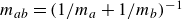 $m_{ab} = (1/m_a + 1/m_b)^{-1}$
, collision time
$m_{ab} = (1/m_a + 1/m_b)^{-1}$
, collision time
 $\tau _{{col}}$
, and coefficient of restitution
$\tau _{{col}}$
, and coefficient of restitution
 $e$
, as
$e$
, as
 \begin{align} k &= \frac {m_{ab}}{\tau _{{col}}^2}(\pi ^2+\ln(e)^2), \end{align}
 \begin{align} \eta &= -2 \ln(e) \frac {\sqrt {m_{ab}k}}{\sqrt {\pi ^2+\ln(e)^2}}. \end{align}

Figure 18. Profiles of mean fluid velocity and rms velocity fluctuations at
 ${\textit{Re}}_\delta = 800$
. Solid lines correspond to the grid described in the main text, while dashed lines correspond to the refined grid. Lines colours correspond to phases
${\textit{Re}}_\delta = 800$
. Solid lines correspond to the grid described in the main text, while dashed lines correspond to the refined grid. Lines colours correspond to phases
 $\omega t =0^\circ$
(
$\omega t =0^\circ$
(
![]() ),
),
 $\omega t =30^\circ$
(
$\omega t =30^\circ$
(
![]() ),
),
 $\omega t =60^\circ$
(
$\omega t =60^\circ$
(
![]() ),
),
 $\omega t =90^\circ$
(
$\omega t =90^\circ$
(
![]() ),
),
 $\omega t =120^\circ$
(
$\omega t =120^\circ$
(
![]() ), and
), and
 $\omega t =150^\circ$
(
$\omega t =150^\circ$
(
![]() ). The agreement is close, showing that the simulation is grid converged.
). The agreement is close, showing that the simulation is grid converged.
The radius of influence
 $\lambda$
allows us to robustly handle high-speed collisions by initiating the collision of high-speed particle pairs just before contact. Following Finn et al. (Reference Finn, Li and Apte2016),
$\lambda$
allows us to robustly handle high-speed collisions by initiating the collision of high-speed particle pairs just before contact. Following Finn et al. (Reference Finn, Li and Apte2016),
 $\lambda$
is calculated as
$\lambda$
is calculated as
 \begin{equation} \lambda = \frac {\lambda _0}{2}(d_{p,a}+d_{p,b})\left ( \frac {\textrm {CFL}^c_{ab}}{\textrm {CFL}^c_{\textit{max}}} \right ), \end{equation}
where the collisional CFL number is
 $\textrm {CFL}^c_{ab} = (2\, |\boldsymbol{u}_{ab,n}|\, \Delta t)/(d_{\!p}^a+d_{\!p}^b)$
, and
$\textrm {CFL}^c_{ab} = (2\, |\boldsymbol{u}_{ab,n}|\, \Delta t)/(d_{\!p}^a+d_{\!p}^b)$
, and
 $\lambda _0$
is the maximum radius of influence permitted when the collision occurs at the maximum collision CFL number,
$\lambda _0$
is the maximum radius of influence permitted when the collision occurs at the maximum collision CFL number,
 $\textrm {CFL}^c_{\textit{max}}$
. The tangential collision force is modelled according to a static friction model
$\textrm {CFL}^c_{\textit{max}}$
. The tangential collision force is modelled according to a static friction model
 \begin{equation} \boldsymbol{f}_{p,t}^{{c,b\rightarrow a}} = -\mu _s\, |\boldsymbol{f}_{p,t}^{{c,b\rightarrow a}} |\, \boldsymbol{t}_{ab}, \end{equation}
where
 $\boldsymbol{t}_{ab}$
is the tangential direction, and
$\boldsymbol{t}_{ab}$
is the tangential direction, and
 $\mu _s$
is the static friction coefficient. Collisions with walls are treated in the same way as above, but with the wall having infinite mass.
$\mu _s$
is the static friction coefficient. Collisions with walls are treated in the same way as above, but with the wall having infinite mass.
Appendix C. Grid convergence study
In order to demonstrate grid independence, we conduct a simulation at
 ${\textit{Re}}_\delta = 800$
with grid resolution
${\textit{Re}}_\delta = 800$
with grid resolution
 $N_x \times N_y \times N_z = 672 \times 422 \times 134$
, and compare the results to the simulation with resolution
$N_x \times N_y \times N_z = 672 \times 422 \times 134$
, and compare the results to the simulation with resolution
 $N_x \times N_y \times N_z = 672 \times 211 \times 134$
, for one period. Thus the wall-normal resolution is twice that in the coarser grid. Note that we do not refine the grid in the streamwise and spanwise directions because the gradients are primarily in the wall-normal direction, and the resolution in the streamwise and spanwise directions already exceeds the requirements for an OBL over a smooth wall. That is, the resolutions in the smooth wall case described in Appendix A are
$N_x \times N_y \times N_z = 672 \times 211 \times 134$
, for one period. Thus the wall-normal resolution is twice that in the coarser grid. Note that we do not refine the grid in the streamwise and spanwise directions because the gradients are primarily in the wall-normal direction, and the resolution in the streamwise and spanwise directions already exceeds the requirements for an OBL over a smooth wall. That is, the resolutions in the smooth wall case described in Appendix A are
 $0.78 \delta$
and
$0.78 \delta$
and
 $0.39 \delta$
in the streamwise and spanwise directions, respectively, while the resolution is
$0.39 \delta$
in the streamwise and spanwise directions, respectively, while the resolution is
 $0.37 \delta$
in all directions for the bed cases.
$0.37 \delta$
in all directions for the bed cases.
In figure 18, we compare the fluid streamwise velocity profile, streamwise velocity fluctuations, and streamwise particle velocity. Increasing the resolution does not lead to significant change in these statistics. This indicates that our resolution choice in this study is adequate up to
 ${\textit{Re}}_\delta =800$
.
${\textit{Re}}_\delta =800$
.
Appendix D. Validation of the present Euler–Lagrange method for sediment transport
To demonstrate the capability of the present model to capture accurate sediment transport, we reproduce numerically the experiments of Aussillous et al. (Reference Aussillous, Chauchat, Pailha, Médale and Guazzelli2013) of bedload transport in a channel flow.
Following earlier numerical effort in Kidanemariam & Uhlmann (Reference Kidanemariam and Uhlmann2014), Charru et al. (Reference Charru, Bouteloup, Bonometti and Lacaze2016) and Rao & Capecelatro (Reference Rao and Capecelatro2019), we set up our numerical analogue as shown in figure 19(a). The sediment grains are monodisperse with diameter
 $d_{\!p}$
, restitution coefficient
$d_{\!p}$
, restitution coefficient
 $e=0.3$
, and friction coefficient
$e=0.3$
, and friction coefficient
 $\mu _c=0.4$
(Kidanemariam & Uhlmann Reference Kidanemariam and Uhlmann2014). The domain dimensions are
$\mu _c=0.4$
(Kidanemariam & Uhlmann Reference Kidanemariam and Uhlmann2014). The domain dimensions are
 $32d_{\!p}$
in the streamwise direction,
$32d_{\!p}$
in the streamwise direction,
 $32d_{\!p}$
in the vertical direction, and
$32d_{\!p}$
in the vertical direction, and
 $16d_{\!p}$
in the spanwise direction. We use a uniform grid with spacing
$16d_{\!p}$
in the spanwise direction. We use a uniform grid with spacing
 $\Delta x=d_{\!p}/2$
, the same as in the main study.
$\Delta x=d_{\!p}/2$
, the same as in the main study.

Figure 19. Sediment transport in a laminar channel flow: (a) schematic of the configuration in our simulations, and (b) variation of the normalised sediment flow rate with Shields number. The PR-DNS data are from Kidanemariam & Uhlmann (Reference Kidanemariam and Uhlmann2014). The experimental data are from Aussillous et al. (Reference Aussillous, Chauchat, Pailha, Médale and Guazzelli2013). Despite not capturing flow features at the particle scale, our method captures the variation of sediment transport with Shields number very well.
The main non-dimensional numbers that control this problem are the bulk Reynolds number
 ${\textit{Re}}=q_{\!f}/\nu$
, where
${\textit{Re}}=q_{\!f}/\nu$
, where
 $q_{\!f}$
is the fluid flow rate, Galileo number
$q_{\!f}$
is the fluid flow rate, Galileo number
 ${\textit{Ga}}$
, density ratio
${\textit{Ga}}$
, density ratio
 $\rho _{\!p}/\rho _{\!f}$
, and Shields number
$\rho _{\!p}/\rho _{\!f}$
, and Shields number
 $\theta$
. Following Kidanemariam & Uhlmann (Reference Kidanemariam and Uhlmann2014), Charru et al. (Reference Charru, Bouteloup, Bonometti and Lacaze2016) and Rao & Capecelatro (Reference Rao and Capecelatro2019), and to enable comparisons with Aussillous et al. (Reference Aussillous, Chauchat, Pailha, Médale and Guazzelli2013), we define the Shields number based on the wall shear stress from a laminar Poiseuille flow. As discussed by Kidanemariam & Uhlmann (Reference Kidanemariam and Uhlmann2014), this results in the following expression for the Shields number:
$\theta$
. Following Kidanemariam & Uhlmann (Reference Kidanemariam and Uhlmann2014), Charru et al. (Reference Charru, Bouteloup, Bonometti and Lacaze2016) and Rao & Capecelatro (Reference Rao and Capecelatro2019), and to enable comparisons with Aussillous et al. (Reference Aussillous, Chauchat, Pailha, Médale and Guazzelli2013), we define the Shields number based on the wall shear stress from a laminar Poiseuille flow. As discussed by Kidanemariam & Uhlmann (Reference Kidanemariam and Uhlmann2014), this results in the following expression for the Shields number:
 \begin{equation} \theta =\frac {6\,{\textit{Re}}}{{\textit{Ga}}^2}\left (\frac {d_{\!p}}{H_{\!f}}\right )^2. \end{equation}
Note that we determine the fluid column height
 $H_{\!f}$
using the same approach outlined in Kidanemariam & Uhlmann (Reference Kidanemariam and Uhlmann2014) and Rao & Capecelatro (Reference Rao and Capecelatro2019).
$H_{\!f}$
using the same approach outlined in Kidanemariam & Uhlmann (Reference Kidanemariam and Uhlmann2014) and Rao & Capecelatro (Reference Rao and Capecelatro2019).
Following Kidanemariam & Uhlmann (Reference Kidanemariam and Uhlmann2014), we fix the bulk Reynolds number at
 ${\textit{Re}}=375$
, density ratio at
${\textit{Re}}=375$
, density ratio at
 $\rho _{\!p}/\rho _{\!f}=2.5$
, and Galileo number at
$\rho _{\!p}/\rho _{\!f}=2.5$
, and Galileo number at
 ${\textit{Ga}}=8.56$
. We vary the Shields number from
${\textit{Ga}}=8.56$
. We vary the Shields number from
 $0.05$
to
$0.05$
to
 $0.35$
by varying the bed height
$0.35$
by varying the bed height
 $H_b$
. Similar to the main study, we drive the flow using a pressure gradient forcing, which is constant here. The flow reaches a steady state after approximately
$H_b$
. Similar to the main study, we drive the flow using a pressure gradient forcing, which is constant here. The flow reaches a steady state after approximately
 $200 H_b/U_b$
, where
$200 H_b/U_b$
, where
 $U_b$
is the bulk velocity, at which point we start collecting data.
$U_b$
is the bulk velocity, at which point we start collecting data.
Despite not resolving flow features at the particle scale, the methodology and computational methods outlined in this paper are well capable of reproducing meso-scale dynamics, including bedload sediment transport. This is well evidenced in figure 19(b), which shows the variation of the normalised sediment
 $q_s/({\textit{Ga}}^2\nu )$
flux with Shields number. The figure shows our data alongside data from the experiments of Aussillous et al. (Reference Aussillous, Chauchat, Pailha, Médale and Guazzelli2013), PR-DNS of Kidanemariam & Uhlmann (Reference Kidanemariam and Uhlmann2014), and their correlation
$q_s/({\textit{Ga}}^2\nu )$
flux with Shields number. The figure shows our data alongside data from the experiments of Aussillous et al. (Reference Aussillous, Chauchat, Pailha, Médale and Guazzelli2013), PR-DNS of Kidanemariam & Uhlmann (Reference Kidanemariam and Uhlmann2014), and their correlation
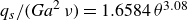 $q_s/({\textit{Ga}}^2\,\nu ) = 1.6584\, \theta ^{3.08}$
. As is clearly shown in figure 19(b), the present methodology yields good agreement with experimental and PR-DNS data. The variation of the normalised sediment flow rate is well captured across three orders of magnitude. It follows a cubic law, similar to the one determined by Kidanemariam & Uhlmann (Reference Kidanemariam and Uhlmann2014) and noted in other studies (Leighton & Acrivos Reference Leighton and Acrivos1986; Charru & Mouilleron-Arnould Reference Charru and Mouilleron-Arnould2002; Charru et al. Reference Charru, Bouteloup, Bonometti and Lacaze2016). This validates our approach for the problem in this study.
$q_s/({\textit{Ga}}^2\,\nu ) = 1.6584\, \theta ^{3.08}$
. As is clearly shown in figure 19(b), the present methodology yields good agreement with experimental and PR-DNS data. The variation of the normalised sediment flow rate is well captured across three orders of magnitude. It follows a cubic law, similar to the one determined by Kidanemariam & Uhlmann (Reference Kidanemariam and Uhlmann2014) and noted in other studies (Leighton & Acrivos Reference Leighton and Acrivos1986; Charru & Mouilleron-Arnould Reference Charru and Mouilleron-Arnould2002; Charru et al. Reference Charru, Bouteloup, Bonometti and Lacaze2016). This validates our approach for the problem in this study.


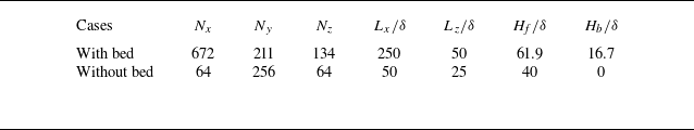


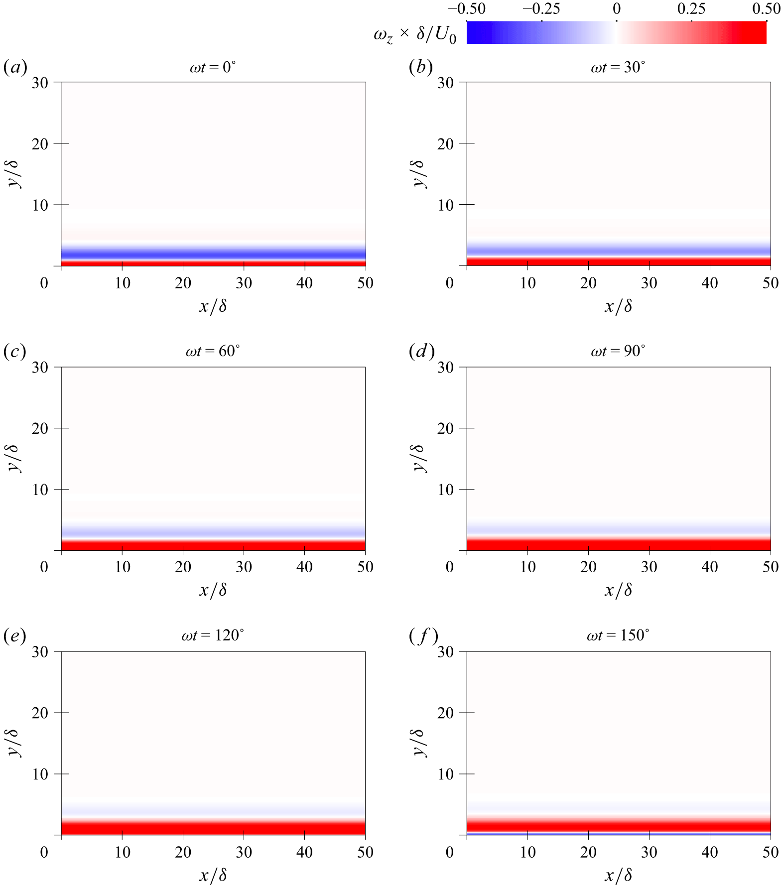


 Open access