


1 Introduction
Let n be a positive integer and let $G=GL_n({\mathbb {C}})$
. Given positive integers
$G=GL_n({\mathbb {C}})$
. Given positive integers $p,q$
such that
$p,q$
such that $p+q=n$
, let K be a Levi subgroup of the stabilizer in G of a p-dimensional subspace of
$p+q=n$
, let K be a Levi subgroup of the stabilizer in G of a p-dimensional subspace of ${\mathbb {C}}^n$
. So,
${\mathbb {C}}^n$
. So, $K \cong GL_p({\mathbb {C}}) \times GL_q({\mathbb {C}})$
. Then K is spherical. We examine coincidences between two well-studied classes of subvarieties in the type A flag variety: Hessenberg varieties and K-orbit closures. We identify a collection of Hessenberg varieties, each equal to the closure of a single K-orbit. Leveraging the theory of K-orbits, we answer, for this particular collection, questions that are difficult to settle for arbitrary Hessenberg varieties.
$K \cong GL_p({\mathbb {C}}) \times GL_q({\mathbb {C}})$
. Then K is spherical. We examine coincidences between two well-studied classes of subvarieties in the type A flag variety: Hessenberg varieties and K-orbit closures. We identify a collection of Hessenberg varieties, each equal to the closure of a single K-orbit. Leveraging the theory of K-orbits, we answer, for this particular collection, questions that are difficult to settle for arbitrary Hessenberg varieties.
Let B be the Borel subgroup of G consisting of upper triangular matrices. The flag variety $\mathcal {B}=G/B$
has been studied extensively since the 1950s. More recently, Hessenberg varieties in
$\mathcal {B}=G/B$
has been studied extensively since the 1950s. More recently, Hessenberg varieties in $\mathcal {B}$
, which were first studied due to their connection with numerical linear algebra, have been of interest to geometers, representation theorists and combinatorialists.
$\mathcal {B}$
, which were first studied due to their connection with numerical linear algebra, have been of interest to geometers, representation theorists and combinatorialists.
We identify $\mathcal {B}$
with the collection of full flags
$\mathcal {B}$
with the collection of full flags
 $$ \begin{align*}V_\bullet=0<V_1<\ldots<V_{n-1}<V_n={\mathbb{C}}^n \end{align*} $$
with $\dim V_i=i$
for all
$\dim V_i=i$
for all $i \in [n]:=\{1,\dots , n\}$
. A Hessenberg vector is a weakly increasing sequence
$i \in [n]:=\{1,\dots , n\}$
. A Hessenberg vector is a weakly increasing sequence ${\mathbf m}=(m_1,\ldots ,m_n)$
of integers satisfying
${\mathbf m}=(m_1,\ldots ,m_n)$
of integers satisfying $i \leq m_i \leq n$
for each
$i \leq m_i \leq n$
for each $i \in [n]$
. Given such
$i \in [n]$
. Given such ${\mathbf m}$
and any
${\mathbf m}$
and any $n \times n$
matrix
$n \times n$
matrix $\mathsf {x}$
, the associated Hessenberg variety is
$\mathsf {x}$
, the associated Hessenberg variety is
 $$ \begin{align*}\mathrm{Hess}(\mathsf{x},{\mathbf m}):=\{V_\bullet \in \mathcal{B} \mid \mathsf{x} V_i \leq V_{m_i} \mbox{ for all } i \in [n]\}. \end{align*} $$
While there have been more recent developments, the survey [Reference Abe and HoriguchiAH20] by Abe and Horiguchi gives a nice summary of the work on Hessenberg varieties and connections to various fields.
Despite their elementary definition, some basic questions about the structure of Hessenberg varieties remain wide open. The ones of interest herein follow.
-
(A) What is the dimension of $\mathrm {Hess}(\mathsf {x},{\mathbf m})$
?
$\mathrm {Hess}(\mathsf {x},{\mathbf m})$
? -
(B) For which matrices
$\mathsf {x}$
and Hessenberg vectors
${\mathbf m}$
is
$\mathrm {Hess}(\mathsf {x},{\mathbf m})$
irreducible? -
(C) If
$\mathrm {Hess}(\mathsf {x},{\mathbf m})$
is irreducible, can we describe cohomology class in
$H^\ast (\mathcal {B}; {\mathbb {Z}})$
it represents?


Let us give an example illustrating that Questions (A) and (B) are subtle, in that their answers can depend on the choice of matrix $\mathsf {x}$
when
$\mathsf {x}$
when ${\mathbf m}$
is fixed.
${\mathbf m}$
is fixed.
Example 1. Consider the Hessenberg vector ${\mathbf m}=(2,3,4,\ldots ,n,n)$
. If
${\mathbf m}=(2,3,4,\ldots ,n,n)$
. If ${\mathsf s}$
is a regular semisimple matrix, then by the work of De Mari, Procesi and Shayman in [Reference De Mari, Procesi and ShaymanMPS92],
${\mathsf s}$
is a regular semisimple matrix, then by the work of De Mari, Procesi and Shayman in [Reference De Mari, Procesi and ShaymanMPS92], $\mathrm {Hess}({\mathsf s},{\mathbf m})$
is isomorphic to the toric variety associated to the fan of type
$\mathrm {Hess}({\mathsf s},{\mathbf m})$
is isomorphic to the toric variety associated to the fan of type $A_{n-1}$
Weyl chambers. In particular,
$A_{n-1}$
Weyl chambers. In particular, $\mathrm {Hess}({\mathsf s},{\mathbf m})$
is irreducible of dimension
$\mathrm {Hess}({\mathsf s},{\mathbf m})$
is irreducible of dimension $n-1$
.
$n-1$
.
Example 2. Let ${\mathbf m} = (2,3,4,\ldots ,n,n)$
as in Example 1. For
${\mathbf m} = (2,3,4,\ldots ,n,n)$
as in Example 1. For $i \in [n-1]$
, let
$i \in [n-1]$
, let $w^i \in {\mathbf {S}}_n$
be the unique permutation satisfying
$w^i \in {\mathbf {S}}_n$
be the unique permutation satisfying
-
•
$w^i(1)=i+1$
, -
•
$w^i(n)=i$
, and -
•
$w^i(j)>w^i(j+1)$
for
$2 \leq j \leq n-2$
.


We write $E_{1n}$
for the
$E_{1n}$
for the $n \times n$
elementary matrix whose only nonzero entry is in its first row and last column. As shown by Tymoczko in [Reference TymoczkoTym06],
$n \times n$
elementary matrix whose only nonzero entry is in its first row and last column. As shown by Tymoczko in [Reference TymoczkoTym06], $\mathrm {Hess}(E_{1n},{\mathbf m})$
is the union of the Schubert varieties
$\mathrm {Hess}(E_{1n},{\mathbf m})$
is the union of the Schubert varieties $X_{w^i}$
, from which it follows that
$X_{w^i}$
, from which it follows that $\mathrm {Hess}(E_{1n},{\mathbf m})$
has
$\mathrm {Hess}(E_{1n},{\mathbf m})$
has $n-1$
irreducible components, each of dimension
$n-1$
irreducible components, each of dimension $1+{{n-1} \choose {2}}.$
Remark 3. For a fixed Hessenberg vector ${\mathbf m}$
, there can be irreducible varieties
${\mathbf m}$
, there can be irreducible varieties $\mathrm {Hess}(\mathsf {x},{\mathbf m})$
and
$\mathrm {Hess}(\mathsf {x},{\mathbf m})$
and $\mathrm {Hess}({\mathsf y},{\mathbf m})$
of differing dimensions. For example, if
$\mathrm {Hess}({\mathsf y},{\mathbf m})$
of differing dimensions. For example, if $m_1<n$
and
$m_1<n$
and $m_j=n$
for
$m_j=n$
for $j>1$
, then
$j>1$
, then $\mathrm {Hess}(\mathsf {x},{\mathbf m})=\mathcal {B}$
if and only if
$\mathrm {Hess}(\mathsf {x},{\mathbf m})=\mathcal {B}$
if and only if $\mathsf {x}$
is scalar, while
$\mathsf {x}$
is scalar, while $\mathrm {Hess}({\mathsf y},{\mathbf m})$
is irreducible of dimension
$\mathrm {Hess}({\mathsf y},{\mathbf m})$
is irreducible of dimension $\dim (\mathcal {B}) - (n-m_1)$
whenever
$\dim (\mathcal {B}) - (n-m_1)$
whenever ${\mathsf y}$
is regular.
${\mathsf y}$
is regular.
The results on $\mathrm {Hess}(E_{1n},(2,3,\ldots ,n,n))$
discussed in Example 2 are worth further consideration. The key point is that for each
$\mathrm {Hess}(E_{1n},(2,3,\ldots ,n,n))$
discussed in Example 2 are worth further consideration. The key point is that for each $g \in B$
,
$g \in B$
, $E_{1n}g=\lambda gE_{1n}$
for some
$E_{1n}g=\lambda gE_{1n}$
for some $\lambda \in {\mathbb {C}}$
. That is, the Borel subgroup B stabilizes the subspace spanned by
$\lambda \in {\mathbb {C}}$
. That is, the Borel subgroup B stabilizes the subspace spanned by $ E_{1n}$
under the adjoint action. It follows directly that for every Hessenberg vector
$ E_{1n}$
under the adjoint action. It follows directly that for every Hessenberg vector ${\mathbf m}$
,
${\mathbf m}$
, $\mathrm {Hess}(E_{1n},{\mathbf m})$
is B-invariant and therefore a union of B-orbits. Thus, every irreducible component of
$\mathrm {Hess}(E_{1n},{\mathbf m})$
is B-invariant and therefore a union of B-orbits. Thus, every irreducible component of $\mathrm {Hess}(E_{1n},{\mathbf m})$
is a Schubert variety
$\mathrm {Hess}(E_{1n},{\mathbf m})$
is a Schubert variety $X_w$
for some
$X_w$
for some $w \in {\mathbf {S}}_n$
. One can determine which
$w \in {\mathbf {S}}_n$
. One can determine which $X_w$
appear as such components for any given
$X_w$
appear as such components for any given ${\mathbf m}$
; see [Reference TymoczkoTym06, Reference Abe and CrooksAC16].
${\mathbf m}$
; see [Reference TymoczkoTym06, Reference Abe and CrooksAC16].
We use the approach described in the previous paragraph to study $\mathrm {Hess}(\mathsf {x},{\mathbf m})$
when
$\mathrm {Hess}(\mathsf {x},{\mathbf m})$
when $\mathsf {x}$
is semisimple with exactly two distinct eigenvalues. Given such
$\mathsf {x}$
is semisimple with exactly two distinct eigenvalues. Given such $\mathsf {x}$
with eigenvalues
$\mathsf {x}$
with eigenvalues $\lambda ,\mu $
of respective multiplicities
$\lambda ,\mu $
of respective multiplicities $p,q$
(hence
$p,q$
(hence $p+q=n$
), let
$p+q=n$
), let $Y,Z$
be the associated eigenspaces. Thus,
$Y,Z$
be the associated eigenspaces. Thus, ${\mathbb {C}}^n=Y \oplus Z$
. The simultaneous stabilizer K of Y and Z in G is isomorphic to
${\mathbb {C}}^n=Y \oplus Z$
. The simultaneous stabilizer K of Y and Z in G is isomorphic to $GL_p({\mathbb {C}}) \times GL_q({\mathbb {C}})$
, and it is straightforward to see that
$GL_p({\mathbb {C}}) \times GL_q({\mathbb {C}})$
, and it is straightforward to see that $\mathrm {Hess}(\mathsf {x},{\mathbf m})$
is a union of K-orbits. It is well known (see, for example, [Reference WolfWol69]) that K is spherical; that is, K has finitely many orbits on
$\mathrm {Hess}(\mathsf {x},{\mathbf m})$
is a union of K-orbits. It is well known (see, for example, [Reference WolfWol69]) that K is spherical; that is, K has finitely many orbits on $\mathcal {B}$
. We will use the classification and theory of K-orbits on
$\mathcal {B}$
. We will use the classification and theory of K-orbits on $\mathcal {B}$
due to Yamamoto [Reference YamamotoYam97] and many others [Reference Matsuki and ŌshimaMO90, Reference WyserWys16, Reference Can and UğurluCU19] to address Questions (A), (B), (C) above for Hessenberg varieties defined using such
$\mathcal {B}$
due to Yamamoto [Reference YamamotoYam97] and many others [Reference Matsuki and ŌshimaMO90, Reference WyserWys16, Reference Can and UğurluCU19] to address Questions (A), (B), (C) above for Hessenberg varieties defined using such $\mathsf {x}$
.
$\mathsf {x}$
.
Assume as above that the semisimple matrix $\mathsf {x}$
has exactly two distinct eigenvalues
$\mathsf {x}$
has exactly two distinct eigenvalues $\lambda ,\mu $
with respective multiplicities
$\lambda ,\mu $
with respective multiplicities $p,q$
, and fix a Hessenberg vector
$p,q$
, and fix a Hessenberg vector ${\mathbf m}$
. We observe that the isomorphism type of
${\mathbf m}$
. We observe that the isomorphism type of $\mathrm {Hess}(\mathsf {x},{\mathbf m})$
depends only on p and q. Indeed, since
$\mathrm {Hess}(\mathsf {x},{\mathbf m})$
depends only on p and q. Indeed, since $\mathrm {Hess}(g^{-1}\mathsf {x} g,{\mathbf m})=g\mathrm {Hess}(\mathsf {x},{\mathbf m})$
for every
$\mathrm {Hess}(g^{-1}\mathsf {x} g,{\mathbf m})=g\mathrm {Hess}(\mathsf {x},{\mathbf m})$
for every $g \in G$
, we may assume that
$g \in G$
, we may assume that $\mathsf {x}=(x_{ij})$
is diagonal with
$\mathsf {x}=(x_{ij})$
is diagonal with $x_{ii}=\lambda $
for
$x_{ii}=\lambda $
for $i \in [p]$
and
$i \in [p]$
and $x_{ii}=\mu $
for
$x_{ii}=\mu $
for $p<i \leq n$
. Moreover, it is straightforward to show that for scalars
$p<i \leq n$
. Moreover, it is straightforward to show that for scalars $\alpha \neq 0$
and
$\alpha \neq 0$
and $\beta $
,
$\beta $
,
 $$ \begin{align*}\mathrm{Hess}(\alpha\mathsf{x}+\beta I,{\mathbf m})=\mathrm{Hess}(\mathsf{x},{\mathbf m}); \end{align*} $$
hence, $\lambda $
and
$\lambda $
and $\mu $
are irrelevant and our observation follows. So, there is no harm in writing
$\mu $
are irrelevant and our observation follows. So, there is no harm in writing $\mathsf {x}_{p,q}$
to denote any such semisimple matrix
$\mathsf {x}_{p,q}$
to denote any such semisimple matrix $\mathsf {x}$
.
$\mathsf {x}$
.
We summarize now our results on $\mathrm {Hess}(\mathsf {x}_{p,q},{\mathbf m})$
. Our first result addresses Question (B).
$\mathrm {Hess}(\mathsf {x}_{p,q},{\mathbf m})$
. Our first result addresses Question (B).
Theorem 4 (See Corollaries 3.7 and 3.9 and Theorem 3.11 below).
The following conditions on the Hessenberg variety $\mathrm {Hess}(\mathsf {x}_{p,q},{\mathbf m})$
are equivalent.
$\mathrm {Hess}(\mathsf {x}_{p,q},{\mathbf m})$
are equivalent.
-
1.
$\mathrm {Hess}(\mathsf {x}_{p,q},{\mathbf m})$
is irreducible. -
2. There is a Hessenberg vector
$(\ell _1,\ldots ,\ell _q)$
of length q such that
$m_i=\ell _i+p$
for
$i \leq q$
and
$m_i=n$
for
$q<i \leq n$
. -
3.
$\mathrm {Hess}(\mathsf {x}_{p,q}, {\mathbf m})$
is the closure of one of
$\frac {1}{q+1}{{2q} \choose {q}}$
orbits of K on
$\mathcal {B}$
. This collection of orbits is naturally parameterized by
$231$
-free permutations in
${\mathbf {S}}_q$
.


There is a formula for the dimensions of K-orbits in a flag variety (see [Reference YamamotoYam97, Section 2.3]). This formula allows us to compute and write a nice formula for the dimension of any irreducible $\mathrm {Hess}(\mathsf {x}_{p,q},{\mathbf m})$
, thereby addressing Question (A) for this collection.
$\mathrm {Hess}(\mathsf {x}_{p,q},{\mathbf m})$
, thereby addressing Question (A) for this collection.
Corollary 5 (See Corollary 3.14 below).
If ${\mathbf m}=(m_1,\ldots ,m_n)$
is a Hessenberg vector such that
${\mathbf m}=(m_1,\ldots ,m_n)$
is a Hessenberg vector such that $\mathrm {Hess}(\mathsf {x}_{p,q},{\mathbf m})$
is irreducible, then
$\mathrm {Hess}(\mathsf {x}_{p,q},{\mathbf m})$
is irreducible, then
 $$ \begin{align*}\dim\mathrm{Hess}(\mathsf{x}_{p,q},{\mathbf m})=\sum_{i=1}^n(m_i-i). \end{align*} $$
Previous work on Question (C) addresses cases where $\mathsf {x}$
is regular. It is known that the class of any regular Hessenberg variety depends only on the underlying Hessenberg vector [Reference Abe, Fujita and ZengAFZ20]. Polynomial representatives for the classes of regular Hessenberg varieties were first identified as specializations of certain double Schubert polynomials [Reference Anderson and TymoczkoAT10, Reference Insko, Tymoczko and WooITW20]. Even more recently, Nadeau and Tewari [Reference Nadeau and TewariNT21] gave a combinatorial formula expressing each as a sum of Schubert polynomials in the special case of
$\mathsf {x}$
is regular. It is known that the class of any regular Hessenberg variety depends only on the underlying Hessenberg vector [Reference Abe, Fujita and ZengAFZ20]. Polynomial representatives for the classes of regular Hessenberg varieties were first identified as specializations of certain double Schubert polynomials [Reference Anderson and TymoczkoAT10, Reference Insko, Tymoczko and WooITW20]. Even more recently, Nadeau and Tewari [Reference Nadeau and TewariNT21] gave a combinatorial formula expressing each as a sum of Schubert polynomials in the special case of ${\mathbf m}=(2,3,\ldots ,n,n)$
. Here, we consider certain cases in which
${\mathbf m}=(2,3,\ldots ,n,n)$
. Here, we consider certain cases in which $\mathsf {x}$
is not regular.
$\mathsf {x}$
is not regular.
Let us state a more specific version of Question (C). The cohomology classes associated with the Schubert varieties $X_w$
(
$X_w$
( $w \in {\mathbf {S}}_n$
) form a basis for
$w \in {\mathbf {S}}_n$
) form a basis for $H^\ast (\mathcal {B};{\mathbb {Z}})$
. Let I be the ideal in
$H^\ast (\mathcal {B};{\mathbb {Z}})$
. Let I be the ideal in $R:={\mathbb {Z}}[x_1,\ldots ,x_n]$
generated by constant-free symmetric polynomials. There is an isomorphism
$R:={\mathbb {Z}}[x_1,\ldots ,x_n]$
generated by constant-free symmetric polynomials. There is an isomorphism $\phi $
from
$\phi $
from $H^\ast (\mathcal {B};{\mathbb {Z}})$
to
$H^\ast (\mathcal {B};{\mathbb {Z}})$
to $R/I$
mapping the class associated to
$R/I$
mapping the class associated to $X_w$
to the Schubert polynomial
$X_w$
to the Schubert polynomial $\mathfrak {S}_w$
. (This presentation of
$\mathfrak {S}_w$
. (This presentation of $H^\ast (\mathcal {B};{\mathbb {Z}})$
is due to Borel; see [Reference BorelBor53] or [Reference ManivelMan01].) Given any irreducible subvariety
$H^\ast (\mathcal {B};{\mathbb {Z}})$
is due to Borel; see [Reference BorelBor53] or [Reference ManivelMan01].) Given any irreducible subvariety ${\mathcal V}$
of
${\mathcal V}$
of $\mathcal {B}$
, one can ask how to expand the image
$\mathcal {B}$
, one can ask how to expand the image $\mathfrak {S}({\mathcal V})$
under
$\mathfrak {S}({\mathcal V})$
under $\phi $
of the class associated to
$\phi $
of the class associated to ${\mathcal V}$
as a linear combination of Schubert polynomials. We obtain the following result for the collection of irreducible Hessenberg varieties introduced in the statement of Theorem 4.
${\mathcal V}$
as a linear combination of Schubert polynomials. We obtain the following result for the collection of irreducible Hessenberg varieties introduced in the statement of Theorem 4.
Theorem 6 (See Corollary 4.15).
Let $X:=\mathrm {Hess}(\mathsf {x}_{p,q},{\mathbf m})$
be an irreducible Hessenberg variety indexed by a
$X:=\mathrm {Hess}(\mathsf {x}_{p,q},{\mathbf m})$
be an irreducible Hessenberg variety indexed by a $231$
-free permutation
$231$
-free permutation $w\in {\mathbf {S}}_q$
. A polynomial representative of the class
$w\in {\mathbf {S}}_q$
. A polynomial representative of the class $\mathfrak {S}(X)$
of
$\mathfrak {S}(X)$
of $\mathrm {Hess}(\mathsf {x}_{p,q},{\mathbf m})$
in the integral cohomology ring of the flag variety is given by the following sum of Schubert polynomials
$\mathrm {Hess}(\mathsf {x}_{p,q},{\mathbf m})$
in the integral cohomology ring of the flag variety is given by the following sum of Schubert polynomials
 $$ \begin{align*} \mathfrak{S}(X)=\sum_{(u,v)} \mathfrak{S}_{uw_0v^{-1}w_0}, \end{align*} $$
where $w_0$
is the longest element of
$w_0$
is the longest element of $\mathbf{S}_n$
,
$\mathbf{S}_n$
, $y_0$
is the longest element of
$y_0$
is the longest element of $\mathbf{S}_q$
, and the sum is taken over all pairs
$\mathbf{S}_q$
, and the sum is taken over all pairs $(u,v)\in {\mathbf {S}}_q\times {\mathbf {S}}_q$
such that
$(u,v)\in {\mathbf {S}}_q\times {\mathbf {S}}_q$
such that $wy_0 = uv$
and
$wy_0 = uv$
and $\ell (wy_0) = \ell (u)+\ell (v)$
.
$\ell (wy_0) = \ell (u)+\ell (v)$
.
A key ingredient in our computations for Theorem 6 is the useful notion of the W-set associated with a K-orbit $\mathcal {O}=KV_\bullet $
in the flag variety. Loosely speaking, the W-set of
$\mathcal {O}=KV_\bullet $
in the flag variety. Loosely speaking, the W-set of $\mathcal {O}$
consists of permutations that are obtained by multiplying the simple reflections that label the edges of certain saturated paths in the weak order on the spherical variety
$\mathcal {O}$
consists of permutations that are obtained by multiplying the simple reflections that label the edges of certain saturated paths in the weak order on the spherical variety $G/K$
; see Section 2.3 for more. The origins of W-sets go back to the influential work of Richardson and Springer in [Reference Richardson and SpringerRS90], where the authors initiated a systematic study of the (weak) Bruhat orders on the Borel orbit closures in symmetric varieties. This development is generalized by Knop to all spherical homogeneous varieties in [Reference KnopKno95]. Brion’s work [Reference BrionBri01] has brought to light a multitude of fascinating applications of W-sets to the geometry of K-orbits. In particular, Brion used W-sets to describe certain deformations of K-orbits in flag varieties to the unions of Schubert varieties; the results of Theorem 6 rest heavily on this work. More recently, combinatorialists have used W-sets to develop Schubert calculus for (classical) symmetric spaces. There is currently a fast-growing literature on this subject [Reference Wyser and YongWY17, Reference Wyser and YongWY14, Reference Hamaker, Marberg and PawlowskiHMP18, Reference Hamaker and MarbergHM21, Reference Hamaker, Marberg and PawlowskiHMP22].
$G/K$
; see Section 2.3 for more. The origins of W-sets go back to the influential work of Richardson and Springer in [Reference Richardson and SpringerRS90], where the authors initiated a systematic study of the (weak) Bruhat orders on the Borel orbit closures in symmetric varieties. This development is generalized by Knop to all spherical homogeneous varieties in [Reference KnopKno95]. Brion’s work [Reference BrionBri01] has brought to light a multitude of fascinating applications of W-sets to the geometry of K-orbits. In particular, Brion used W-sets to describe certain deformations of K-orbits in flag varieties to the unions of Schubert varieties; the results of Theorem 6 rest heavily on this work. More recently, combinatorialists have used W-sets to develop Schubert calculus for (classical) symmetric spaces. There is currently a fast-growing literature on this subject [Reference Wyser and YongWY17, Reference Wyser and YongWY14, Reference Hamaker, Marberg and PawlowskiHMP18, Reference Hamaker and MarbergHM21, Reference Hamaker, Marberg and PawlowskiHMP22].
It follows directly from Theorem 6 that if $\mathrm {Hess}(\mathsf {x}_{p,q}, {\mathbf m})$
is irreducible, then the polynomial
$\mathrm {Hess}(\mathsf {x}_{p,q}, {\mathbf m})$
is irreducible, then the polynomial $\mathfrak {S}(\mathrm {Hess}(\mathsf {x}_{p,q},{\mathbf m}))$
is a
$\mathfrak {S}(\mathrm {Hess}(\mathsf {x}_{p,q},{\mathbf m}))$
is a $0-1$
sum of Schubert polynomials. In other words, when we express
$0-1$
sum of Schubert polynomials. In other words, when we express $\mathfrak {S}(\mathrm {Hess}(\mathsf {x}_{p,q},{\mathbf m}))$
as a linear combination of Schubert polynomials, all coefficients lie in
$\mathfrak {S}(\mathrm {Hess}(\mathsf {x}_{p,q},{\mathbf m}))$
as a linear combination of Schubert polynomials, all coefficients lie in $\{0,1\}$
. Whenever a polynomial is a
$\{0,1\}$
. Whenever a polynomial is a $0-1$
sum of Schubert polynomials, we say the sum is multiplicity-free. Something stronger is true. For
$0-1$
sum of Schubert polynomials, we say the sum is multiplicity-free. Something stronger is true. For $i \in [n-1]$
, we write
$i \in [n-1]$
, we write $s_i$
for the transposition
$s_i$
for the transposition $(i,i+1) \in {\mathbf {S}}_n$
.
$(i,i+1) \in {\mathbf {S}}_n$
.
Theorem 7 (See Theorem 4.20 below).
If $i \in [n-1]$
and
$i \in [n-1]$
and $\mathrm {Hess}(\mathsf {x}_{p,q}, {\mathbf m})$
is irreducible, then the product
$\mathrm {Hess}(\mathsf {x}_{p,q}, {\mathbf m})$
is irreducible, then the product $\mathfrak {S}_{s_i}\mathfrak {S}(\mathrm {Hess}(\mathsf {x}_{p,q},{\mathbf m}))$
is a multiplicity-free sum of Schubert polynomials.
$\mathfrak {S}_{s_i}\mathfrak {S}(\mathrm {Hess}(\mathsf {x}_{p,q},{\mathbf m}))$
is a multiplicity-free sum of Schubert polynomials.
Theorem 7, which is a consequence of Theorem 6 and Monk’s formula, gives insight into how $\mathrm {Hess}(\mathsf {x}_{p,q},{\mathbf m})$
intersects certain Schubert varieties of codimension one in
$\mathrm {Hess}(\mathsf {x}_{p,q},{\mathbf m})$
intersects certain Schubert varieties of codimension one in $\mathcal {B}$
.
$\mathcal {B}$
.
Geometrically speaking, at the cycle level, the classical Monk’s formula ([Reference MonkMon59, Theorem 3]) says that the intersection of a Schubert variety $X\subseteq G/B$
with a Schubert divisor
$X\subseteq G/B$
with a Schubert divisor $Z \subset G/B$
is a multiplicity-free sum of Schubert divisors of X. Although
$Z \subset G/B$
is a multiplicity-free sum of Schubert divisors of X. Although $\mathrm {Hess}(\mathsf {x}_{p,q},{\mathbf m})$
has a flat degeneration to a union Y of (many) Schubert varieties, it is not a B-stable subvariety of
$\mathrm {Hess}(\mathsf {x}_{p,q},{\mathbf m})$
has a flat degeneration to a union Y of (many) Schubert varieties, it is not a B-stable subvariety of $G/B$
. In light of this fact, we find it rather surprising that the cohomology class of the intersection of
$G/B$
. In light of this fact, we find it rather surprising that the cohomology class of the intersection of $\mathrm {Hess}(\mathsf {x}_{p,q},{\mathbf m})$
with Z is a
$\mathrm {Hess}(\mathsf {x}_{p,q},{\mathbf m})$
with Z is a $0-1$
sum of the classes of Schubert divisors in Y. It is unknown to us if this multiplicity-free phenomenon persists in all cases of the intersection between Z and any K-orbit closure or any irreducible semisimple Hessenberg variety in the flag variety.
$0-1$
sum of the classes of Schubert divisors in Y. It is unknown to us if this multiplicity-free phenomenon persists in all cases of the intersection between Z and any K-orbit closure or any irreducible semisimple Hessenberg variety in the flag variety.
It is natural to ask whether the methods used here and illustrated in Example 2 are more widely applicable. The key idea is that if $\mathrm {Hess}(\mathsf {x},{\mathbf m})$
is invariant under the action of a spherical group H, then known combinatorial descriptions of H-orbits allow for a detailed analysis of
$\mathrm {Hess}(\mathsf {x},{\mathbf m})$
is invariant under the action of a spherical group H, then known combinatorial descriptions of H-orbits allow for a detailed analysis of $\mathrm {Hess}(\mathsf {x},{\mathbf m})$
that is difficult to carry out for arbitrary Hessenberg varieties. If a spherical subgroup H of G centralizes
$\mathrm {Hess}(\mathsf {x},{\mathbf m})$
that is difficult to carry out for arbitrary Hessenberg varieties. If a spherical subgroup H of G centralizes $\mathsf {x}$
(up to multiplication by a scalar), then H indeed acts on
$\mathsf {x}$
(up to multiplication by a scalar), then H indeed acts on $\mathrm {Hess}(\mathsf {x},{\mathbf m})$
for all
$\mathrm {Hess}(\mathsf {x},{\mathbf m})$
for all ${\mathbf m}$
. However, this situation is rare. If
${\mathbf m}$
. However, this situation is rare. If $\mathsf {x}$
is semisimple, then
$\mathsf {x}$
is semisimple, then $C_G(\mathsf {x})$
is reductive. The reductive spherical subgroups of G are known (see [Reference KrämerKrä79],[Reference BrionBri87],[Reference MikityukMik86]). These are the centralizers of the matrices
$C_G(\mathsf {x})$
is reductive. The reductive spherical subgroups of G are known (see [Reference KrämerKrä79],[Reference BrionBri87],[Reference MikityukMik86]). These are the centralizers of the matrices $\mathsf {x}_{p,q}$
studied herein along with the classical groups that act irreducibly on
$\mathsf {x}_{p,q}$
studied herein along with the classical groups that act irreducibly on ${\mathbb {C}}^n$
. In the second case, the centralizer of every such classical group consists of the scalar matrices, and if
${\mathbb {C}}^n$
. In the second case, the centralizer of every such classical group consists of the scalar matrices, and if $\mathsf {x}$
is scalar, then
$\mathsf {x}$
is scalar, then $\mathrm {Hess}(\mathsf {x},{\mathbf m})=\mathcal {B}$
for all
$\mathrm {Hess}(\mathsf {x},{\mathbf m})=\mathcal {B}$
for all ${\mathbf m}$
. There are nilpotent matrices other than conjugates of
${\mathbf m}$
. There are nilpotent matrices other than conjugates of $E_{1n}$
with spherical centralizers in G, but these are also rare. The automorphism group of
$E_{1n}$
with spherical centralizers in G, but these are also rare. The automorphism group of $\mathrm {Hess}(\mathsf {x},{\mathbf m})$
can be much larger than
$\mathrm {Hess}(\mathsf {x},{\mathbf m})$
can be much larger than $C_G(\mathsf {x})$
, but it seems challenging to give a comprehensive and useful analysis of this phenomenon. On the other hand, in [Reference De Mari, Procesi and ShaymanMPS92], De Mari, Procesi and Shayman define Hessenberg varieties for arbitrary reductive groups. In Lie types other than A, there are additional examples of reductive spherical subgroups centralizing nonscalar elements. We will examine these examples in future work.
$C_G(\mathsf {x})$
, but it seems challenging to give a comprehensive and useful analysis of this phenomenon. On the other hand, in [Reference De Mari, Procesi and ShaymanMPS92], De Mari, Procesi and Shayman define Hessenberg varieties for arbitrary reductive groups. In Lie types other than A, there are additional examples of reductive spherical subgroups centralizing nonscalar elements. We will examine these examples in future work.
2 Notation and preliminaries
We review here various results and definitions that we will use below. We denote by ${\mathbb {Z}}_+$
the set of positive integers. Let
${\mathbb {Z}}_+$
the set of positive integers. Let $n\in {\mathbb {Z}}_+$
. Let
$n\in {\mathbb {Z}}_+$
. Let $G=GL_n({\mathbb {C}})$
and let
$G=GL_n({\mathbb {C}})$
and let $B \leq G$
be the Borel subgroup consisting of upper triangular matrices. The flag variety
$B \leq G$
be the Borel subgroup consisting of upper triangular matrices. The flag variety $G/B$
will be denoted by
$G/B$
will be denoted by $\mathcal {B}$
. We identify each coset
$\mathcal {B}$
. We identify each coset $gB \in \mathcal {B}$
with the flag
$gB \in \mathcal {B}$
with the flag
 $$ \begin{align*}V_\bullet=0<V_1<\ldots <V_{n-1}<V_n={\mathbb{C}}^n \end{align*} $$
in which each $V_i$
is spanned by the first i columns of g.
$V_i$
is spanned by the first i columns of g.
Denote the symmetric group on $[n]$
by
$[n]$
by ${\mathbf {S}}_n$
. Let p and q be positive integers such that
${\mathbf {S}}_n$
. Let p and q be positive integers such that $n=p+q$
. We frequently consider below the smaller symmetric group
$n=p+q$
. We frequently consider below the smaller symmetric group ${\mathbf {S}}_q$
, which we identify with the subgroup of
${\mathbf {S}}_q$
, which we identify with the subgroup of ${\mathbf {S}}_n$
stabilizing
${\mathbf {S}}_n$
stabilizing $[n] \setminus [q]$
pointwise. For
$[n] \setminus [q]$
pointwise. For $i \in [n-1]$
, we write
$i \in [n-1]$
, we write $s_i$
for the simple reflection
$s_i$
for the simple reflection $(i,i+1) \in {\mathbf {S}}_n$
. A reduced word for
$(i,i+1) \in {\mathbf {S}}_n$
. A reduced word for $w \in {\mathbf {S}}_n$
is any shortest possible representation
$w \in {\mathbf {S}}_n$
is any shortest possible representation
 $$ \begin{align*}w=s_{i_1}s_{i_2} \ldots s_{i_\ell} \end{align*} $$
of w as a product of simple reflections. We call the set of simple reflections that appear in any reduced expression of w the support of w and denote it by $\mathrm {Supp}(w)$
. For example,
$\mathrm {Supp}(w)$
. For example, $\mathrm {Supp}(2143) = \mathrm {Supp}(s_1s_3) = \{s_1, s_3\}$
.
$\mathrm {Supp}(2143) = \mathrm {Supp}(s_1s_3) = \{s_1, s_3\}$
.
The length $\ell (w)$
of
$\ell (w)$
of $w\in {\mathbf {S}}_n$
is the number of simple reflections appearing in any reduced word for w. It is well known that
$w\in {\mathbf {S}}_n$
is the number of simple reflections appearing in any reduced word for w. It is well known that
 $$ \begin{align*}\ell(w)=\mid\{i<j \mid 1\leq i<j \leq n,\, w(i)>w(j)\}\mid\end{align*} $$
for all $w\in {\mathbf {S}}_n$
. The longest elements of both
$w\in {\mathbf {S}}_n$
. The longest elements of both ${\mathbf {S}}_n$
and
${\mathbf {S}}_n$
and ${\mathbf {S}}_q$
play a role below; to avoid confusion, we write
${\mathbf {S}}_q$
play a role below; to avoid confusion, we write $w_0$
for the longest element of
$w_0$
for the longest element of ${\mathbf {S}}_n$
and
${\mathbf {S}}_n$
and $y_0$
for the longest element of
$y_0$
for the longest element of ${\mathbf {S}}_q$
.
${\mathbf {S}}_q$
.
We say that $w \in {\mathbf {S}}_n$
avoids
$w \in {\mathbf {S}}_n$
avoids $312$
(or is
$312$
(or is $312$
-free) if there do not exist
$312$
-free) if there do not exist $1 \leq i<j<k \leq n$
such that
$1 \leq i<j<k \leq n$
such that $w(j)<w(k)<w(i)$
and define avoidance of
$w(j)<w(k)<w(i)$
and define avoidance of $231$
similarly. It is straightforward to show that w avoids
$231$
similarly. It is straightforward to show that w avoids $231$
if and only if
$231$
if and only if $w^{-1}$
avoids
$w^{-1}$
avoids $312$
.
$312$
.
2.1 Hessenberg varieties
A Hessenberg vector is a weakly increasing sequence
 $$ \begin{align*}{\mathbf m}=(m_1,\ldots,m_n) \end{align*} $$
of integers satisfying $i \leq m_i \leq n$
for each
$i \leq m_i \leq n$
for each $i \in [n]$
. Given a matrix
$i \in [n]$
. Given a matrix $\mathsf {x}\in \mathfrak {g}:=\mathfrak {gl}_n({\mathbb {C}})$
and Hessenberg vector
$\mathsf {x}\in \mathfrak {g}:=\mathfrak {gl}_n({\mathbb {C}})$
and Hessenberg vector ${\mathbf m}$
, we define the corresponding Hessenberg variety by
${\mathbf m}$
, we define the corresponding Hessenberg variety by
 $$ \begin{align*}\mathrm{Hess}(\mathsf{x},{\mathbf m}) :=\{V_\bullet \in \mathcal{B}\mid \mathsf{x} V_i \leq V_{m_i} \mbox{ for all } i \in [n]\}. \end{align*} $$
Given a Hessenberg vector ${\mathbf m}$
, we define
${\mathbf m}$
, we define $\pi _{\mathbf m}$
to be the lattice path from the upper left corner to the lower right corner of an
$\pi _{\mathbf m}$
to be the lattice path from the upper left corner to the lower right corner of an $n \times n$
grid in which the vertical step in row i occurs in column
$n \times n$
grid in which the vertical step in row i occurs in column $m_i$
. Since
$m_i$
. Since $m_i \geq i$
,
$m_i \geq i$
, $\pi _{\mathbf m}$
is a Dyck path; that is, the lattice path
$\pi _{\mathbf m}$
is a Dyck path; that is, the lattice path $\pi _{\mathbf m}$
never crosses the diagonal connecting the two corners. We write
$\pi _{\mathbf m}$
never crosses the diagonal connecting the two corners. We write $\mathrm {area}(\pi _{\mathbf m})$
for the number of squares in the grid that lie below
$\mathrm {area}(\pi _{\mathbf m})$
for the number of squares in the grid that lie below $\pi _m$
and strictly above the diagonal and observe that
$\pi _m$
and strictly above the diagonal and observe that
 $$ \begin{align*}\mathrm{area}(\pi_{\mathbf m})=\sum_{i=1}^n(m_i-i). \end{align*} $$
Herein, we examine Hessenberg varieties $\mathrm {Hess}(\mathsf {x}_{p,q},{\mathbf m})$
where
$\mathrm {Hess}(\mathsf {x}_{p,q},{\mathbf m})$
where $\mathsf {x}_{\mathfrak {p},q} \in \mathfrak {g}$
is semisimple with exactly two distinct eigenvalues, one of multiplicity p and one of multiplicity q (so
$\mathsf {x}_{\mathfrak {p},q} \in \mathfrak {g}$
is semisimple with exactly two distinct eigenvalues, one of multiplicity p and one of multiplicity q (so $p+q=n$
). Since
$p+q=n$
). Since $\mathrm {Hess}(g^{-1}\mathsf {x} g,{\mathbf m})=g\mathrm {Hess}(\mathsf {x},m)$
for all
$\mathrm {Hess}(g^{-1}\mathsf {x} g,{\mathbf m})=g\mathrm {Hess}(\mathsf {x},m)$
for all $g \in G$
and all
$g \in G$
and all $\mathsf {x} \in \mathfrak {g}$
, we assume without loss of generality that
$\mathsf {x} \in \mathfrak {g}$
, we assume without loss of generality that
 $$ \begin{align*} \mathsf{x}_{p,q} = \text{diag}(\underbrace{\lambda_1,\dots, \lambda_1}_{p \text{ times}}, \underbrace{\lambda_2,\dots, \lambda_2}_{q \text{ times}}), \end{align*} $$
for distinct $\lambda _1,\lambda _2 \in {\mathbb {C}}$
.
$\lambda _1,\lambda _2 \in {\mathbb {C}}$
.
The centralizer of $\mathsf {x}_{p,q}$
in G is the subgroup
$\mathsf {x}_{p,q}$
in G is the subgroup $K \cong GL_p({\mathbb {C}})\times GL_q({\mathbb {C}})$
consisting of all
$K \cong GL_p({\mathbb {C}})\times GL_q({\mathbb {C}})$
consisting of all $g=(g_{ij}) \in G$
such that
$g=(g_{ij}) \in G$
such that $g_{ij}=0$
if either
$g_{ij}=0$
if either $i \leq p<j$
or
$i \leq p<j$
or $j \leq p<i$
. It is straightforward to confirm that if
$j \leq p<i$
. It is straightforward to confirm that if $V_\bullet \in \mathrm {Hess}(\mathsf {x}_{p,q},{\mathbf m})$
and
$V_\bullet \in \mathrm {Hess}(\mathsf {x}_{p,q},{\mathbf m})$
and $g \in K$
, then
$g \in K$
, then
 $$ \begin{align*}gV_\bullet:=0<gV_1<\ldots <gV_{n-1}<{\mathbb{C}}^n \in \mathrm{Hess}(\mathsf{x}_{p,q},{\mathbf m}).\end{align*} $$
Thus, $\mathrm {Hess}(\mathsf {x}_{p,q},{\mathbf m})$
is a union of K-orbits on
$\mathrm {Hess}(\mathsf {x}_{p,q},{\mathbf m})$
is a union of K-orbits on $\mathcal {B}$
.
$\mathcal {B}$
.
2.2 K-orbits on the flag variety
The group K is known to have finitely many orbits on the flag variety $\mathcal {B}$
. These orbits are parameterized by combinatorial objects called clans. Clans originated in work of Matsuki and Ōshima [Reference Matsuki and ŌshimaMO90] to parameterize symmetric subgroup orbits on complex flag manifolds of classical type. Their notation has morphed with developments through subsequent works, notably by Yamamoto [Reference YamamotoYam97] and then Wyser [Reference WyserWys16].
$\mathcal {B}$
. These orbits are parameterized by combinatorial objects called clans. Clans originated in work of Matsuki and Ōshima [Reference Matsuki and ŌshimaMO90] to parameterize symmetric subgroup orbits on complex flag manifolds of classical type. Their notation has morphed with developments through subsequent works, notably by Yamamoto [Reference YamamotoYam97] and then Wyser [Reference WyserWys16].
We define the set of clans as follows. Consider the set of all sequences
 $$ \begin{align*}\gamma=c_1c_2\cdots c_n \end{align*} $$
such that
-
1. each
$c_i$
lies in
$\{+,-\} \cup {\mathbb {Z}}_+$
, -
2. each element of
${\mathbb {Z}}_+$
appearing in
$\gamma $
appears exactly twice, and -
3. if
$+$
and
$-$
appear, respectively, exactly s times and t times in
$\gamma $
, then
$s-t=p-q$
.


We define an equivalence relation on this set by identifying sequences $\gamma =c_1\ldots c_n$
and
$\gamma =c_1\ldots c_n$
and $\delta =d_1\ldots d_n$
if
$\delta =d_1\ldots d_n$
if
-
•
$d_i=d_j \in {\mathbb {Z}}_+$
whenever
$c_i=c_j \in {\mathbb {Z}}_+$
, and -
•
$d_i=c_i$
whenever
$c_i \in \{+,-\}.$


A $(p,q)$
-clan (or clan if
$(p,q)$
-clan (or clan if $p,q$
are fixed) is an equivalence class of this relation. We identify a clan with its unique representative
$p,q$
are fixed) is an equivalence class of this relation. We identify a clan with its unique representative $\gamma $
satisfying
$\gamma $
satisfying
-
• if
$j>1 \in {\mathbb {Z}}_+$
appears in
$\gamma $
, then
$j-1$
appears in
$\gamma $
and the first occurrence of
$j-1$
is to the left of the first occurrence of j,


and write $\mathbf {Clan}_{p,q}$
for the set of all such representatives. So, for example,
$\mathbf {Clan}_{p,q}$
for the set of all such representatives. So, for example, $5++3-+35+$
and
$5++3-+35+$
and $1++2-+21+$
lie in the same
$1++2-+21+$
lie in the same $(6,3)$
-clan, and the second of these is our fixed representative for the equivalence class. In general, if
$(6,3)$
-clan, and the second of these is our fixed representative for the equivalence class. In general, if $\gamma \in \mathbf {Clan}_{p,q}$
, then there is some
$\gamma \in \mathbf {Clan}_{p,q}$
, then there is some $\ell \in {\mathbb {Z}}_{\geq 0}$
such that the integers appearing in
$\ell \in {\mathbb {Z}}_{\geq 0}$
such that the integers appearing in $\gamma $
are exactly those in
$\gamma $
are exactly those in $[\ell ]$
, and if s entries of
$[\ell ]$
, and if s entries of $\gamma $
are plus signs and t entries are minus signs, then
$\gamma $
are plus signs and t entries are minus signs, then $p=\ell +s$
and
$p=\ell +s$
and $q=\ell +t$
.
$q=\ell +t$
.
A flag $V(\gamma )_\bullet $
in
$V(\gamma )_\bullet $
in $\mathcal {B}$
is associated with each clan
$\mathcal {B}$
is associated with each clan $\gamma $
in the next definition.
$\gamma $
in the next definition.
Definition 2.1. Let $e_1,\ldots ,e_n$
be the standard basis for
$e_1,\ldots ,e_n$
be the standard basis for ${\mathbb {C}}^n$
. Given
${\mathbb {C}}^n$
. Given $(p,q)$
-clan
$(p,q)$
-clan $\gamma =c_1\ldots c_n$
, define
$\gamma =c_1\ldots c_n$
, define $v_1,\ldots ,v_n \in {\mathbb {C}}^n$
as follows.
$v_1,\ldots ,v_n \in {\mathbb {C}}^n$
as follows.
-
• If
$c_i$
is the
$k^{th}$
occurrence of
$+$
in
$\gamma $
and exactly
$\ell $
elements of
$[q]$
have appeared at least once among
$c_1, \ldots , c_{i-1}$
, set
$v_i=e_{k+\ell }$
. -
• If
$c_i$
is the
$k^{th}$
occurrence of
$-$
in
$\gamma $
and exactly
$\ell $
elements of
$[q]$
have appeared twice among
$c_1, \ldots , c_{i-1}$
, set
$v_i=e_{p+k+\ell }$
. -
• Say
$c_i=c_j=k \in [q]$
for some
$i<j$
, with exactly r occurrences of
$+$
appearing in
$c_1 \cdots c_{i-1}$
, exactly s occurrences of
$-$
appearing in
$c_1 \cdots c_{j-1}$
, and exactly u elements of
$[q]$
appearing twice in
$c_1\cdots c_{j}$
. Then set
$v_i=e_{k+r}+e_{p+s+u}$
and
$v_j=e_{k+r}-e_{p+s+u}$
.


For $i \in [n]$
, set
$i \in [n]$
, set
 $$ \begin{align*}V(\gamma)_i:={\mathbb{C}}\{v_j \mid j \leq i\}\end{align*} $$
and define
 $$ \begin{align*}V(\gamma)_\bullet:=0<V(\gamma)_1< \ldots < V(\gamma)_{n-1}<{\mathbb{C}}^n \in \mathcal{B}.\end{align*} $$
We observe that, for arbitrary $\gamma $
, each vector
$\gamma $
, each vector $v_i$
used to construct
$v_i$
used to construct $V(\gamma )_\bullet $
is either a standard basis vector or of the form
$V(\gamma )_\bullet $
is either a standard basis vector or of the form $e_r \pm e_s$
with
$e_r \pm e_s$
with $r \in [p]$
and
$r \in [p]$
and $p<s \leq n$
.
$p<s \leq n$
.
Example 2.2. Say $p=5$
,
$p=5$
, $q=3$
, and
$q=3$
, and $\gamma =+1+-2+21$
. Then
$\gamma =+1+-2+21$
. Then $v_1=e_1$
,
$v_1=e_1$
, $v_2=e_2+e_8$
,
$v_2=e_2+e_8$
, $v_3=e_3$
,
$v_3=e_3$
, $v_4=e_6$
,
$v_4=e_6$
, $v_5=e_4+e_7$
,
$v_5=e_4+e_7$
, $v_6=e_5$
,
$v_6=e_5$
, $v_7=e_4-e_7$
, and
$v_7=e_4-e_7$
, and $v_8=e_2-e_8$
.
$v_8=e_2-e_8$
.
Definition 2.3. Given a $(p,q)$
-clan
$(p,q)$
-clan $\gamma $
, we set
$\gamma $
, we set
 $$ \begin{align*}{{\mathcal O}}_\gamma:=KV(\gamma)_\bullet,\end{align*} $$
so ${{\mathcal O}}_\gamma $
is the K-orbit on
${{\mathcal O}}_\gamma $
is the K-orbit on $\mathcal {B}$
containing
$\mathcal {B}$
containing $V(\gamma )_\bullet $
.
$V(\gamma )_\bullet $
.
Lemma 2.4 (Matsuki–Ōshima [Reference Matsuki and ŌshimaMO90]).
Each K-orbit on $\mathcal {B}$
contains a unique flag
$\mathcal {B}$
contains a unique flag $V(\gamma )_\bullet $
; therefore, each K-orbit on
$V(\gamma )_\bullet $
; therefore, each K-orbit on $\mathcal {B}$
is of the form
$\mathcal {B}$
is of the form ${{\mathcal O}}_\gamma $
for some
${{\mathcal O}}_\gamma $
for some $\gamma \in \mathbf {Clan}_{p,q}$
. Furthermore,
$\gamma \in \mathbf {Clan}_{p,q}$
. Furthermore, ${{\mathcal O}}_\gamma ={{\mathcal O}}_\delta $
for
${{\mathcal O}}_\gamma ={{\mathcal O}}_\delta $
for $\gamma ,\delta \in \mathbf {Clan}_{p,q}$
if and only if
$\gamma ,\delta \in \mathbf {Clan}_{p,q}$
if and only if $\gamma =\delta $
.
$\gamma =\delta $
.
Definition 2.5. Given $\gamma , \tau \in \mathbf {Clan}_{p,q}$
we write
$\gamma , \tau \in \mathbf {Clan}_{p,q}$
we write $\gamma \leq \tau $
whenever
$\gamma \leq \tau $
whenever ${{\mathcal O}}_\gamma \subseteq \overline {{{\mathcal O}}_\tau }$
. We call the partial order
${{\mathcal O}}_\gamma \subseteq \overline {{{\mathcal O}}_\tau }$
. We call the partial order $\leq $
the inclusion order on
$\leq $
the inclusion order on $\mathbf {Clan}_{p,q}$
.
$\mathbf {Clan}_{p,q}$
.
We now present a result of Wyser [Reference WyserWys16] characterizing the inclusion order. Given a clan $\gamma =c_1c_2\cdots c_n$
, we define
$\gamma =c_1c_2\cdots c_n$
, we define
-
1.
$\gamma (i;+)$
to be the total number of plus signs and pairs of equal natural numbers occurring among
$c_1\cdots c_i$
, -
2.
$\gamma (i;-)$
to be the total number of minus signs and pairs of equal natural numbers occurring among
$c_1\cdots c_i$
, and -
3.
$\gamma (i,j)$
to be the number of pairs of equal numbers
$c_s=c_t\in {\mathbb {Z}}_+$
with
$s\leq i<j<t$
.


Example 2.6. If $\gamma =+1+-2+21$
as in Example 2.2 above, then
$\gamma =+1+-2+21$
as in Example 2.2 above, then
 $$ \begin{align*}(\gamma(i;+))_{i=1}^n=(1,1,2,2,2,3,4,5), \end{align*} $$
 $$ \begin{align*}(\gamma(i;-))_{i=1}^n=(0,0,0,1,1,1,2,3), \end{align*} $$
and
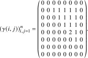 $$ \begin{align*}(\gamma(i,j))_{i,j=1}^n=\left( \begin{array}{cccccccc} 0 & 0 & 0 & 0 & 0 & 0 & 0 & 0 \\ 0 & 0 & 1 & 1 & 1 & 1 & 1 & 0 \\ 0 & 0 & 0 & 1 & 1 & 1 & 1 & 0 \\ 0 & 0 & 0 & 0 & 1 & 1 & 1 & 0 \\ 0 & 0 & 0 & 0 & 0 & 2 & 1 & 0 \\ 0 & 0 & 0 & 0 & 0 & 0 & 1 & 0 \\ 0 & 0 & 0 & 0 & 0 & 0 & 0 & 0 \\ 0 & 0 & 0 & 0 & 0 & 0 & 0 & 0 \end{array} \right). \end{align*} $$
Theorem 2.7 (Wyser).
Let $\gamma $
and
$\gamma $
and $\tau $
be
$\tau $
be $(p,q)$
-clans. Then
$(p,q)$
-clans. Then $\gamma \leq \tau $
if and only if all three inequalities
$\gamma \leq \tau $
if and only if all three inequalities
-
1.
$\gamma (i;+) \geq \tau (i;+)$
, -
2.
$\gamma (i;-) \geq \tau (i; -)$
, and -
3.
$\gamma (i,j) \leq \tau (i,j)$


hold for all $1 \leq i<j \leq n$
.
$1 \leq i<j \leq n$
.
The unique maximum element of $\mathbf {Clan}_{p,q}$
in the inclusion order is
$\mathbf {Clan}_{p,q}$
in the inclusion order is
 $$ \begin{align*}\gamma_0:= 12\cdots q + \cdots + q \cdots 21.\end{align*} $$
(There are $p-q$
plus signs appearing in
$p-q$
plus signs appearing in $\gamma _0$
.) The K-orbit
$\gamma _0$
.) The K-orbit ${{\mathcal O}}_{\gamma _0}$
is open and dense in
${{\mathcal O}}_{\gamma _0}$
is open and dense in $\mathcal {B}$
.
$\mathcal {B}$
.
Example 2.8. We have
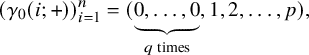 $$\begin{align*}\left(\gamma_0(i;+)\right)_{i=1}^n = (\underbrace{0,\ldots, 0}_{q \text{ times}},1,2,\ldots, p), \end{align*}$$
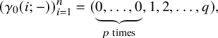 $$\begin{align*}\left(\gamma_0(i;-)\right)_{i=1}^n = (\underbrace{0,\ldots, 0}_{p \text{ times}},1,2,\ldots, q), \end{align*}$$
and
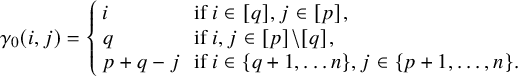 $$ \begin{align*} \gamma_0(i, j)= \left\{\begin{array}{ll}i & \text { if } i \in [q], j \in [p], \\ q & \text { if } i, j \in [p]\backslash[q],\\ p+q-j & \text{ if } i \in\{q+1, \ldots n\}, j \in\{p+1, \ldots, n\}. \\ \end{array} \quad\right. \end{align*} $$
Finally, if $i\in [q]$
and
$i\in [q]$
and $j\in \{p+1, \ldots , n\}$
, then
$j\in \{p+1, \ldots , n\}$
, then $\gamma _0(i,j) = \min \{n-j, i\}$
.
$\gamma _0(i,j) = \min \{n-j, i\}$
.
The following statement, which we record here for use in the next section, follows directly from the definition of the statistic $\gamma (i,j)$
.
$\gamma (i,j)$
.
Lemma 2.9. Let $\gamma \in \mathbf {Clan}_{p,q}$
. For all
$\gamma \in \mathbf {Clan}_{p,q}$
. For all $i>1$
,
$i>1$
, $\gamma (i, j)-\gamma (i-1, j) \in \{0,1\}$
with
$\gamma (i, j)-\gamma (i-1, j) \in \{0,1\}$
with $\gamma (i, j)-\gamma (i-1, j)=1$
if and only if there exists
$\gamma (i, j)-\gamma (i-1, j)=1$
if and only if there exists $t>j$
such that
$t>j$
such that $c_i=c_t$
.
$c_i=c_t$
.
2.3 The weak order
We now recall a formula of Brion for the cohomology class of a K-orbit closure $\overline {{{\mathcal O}}_\gamma }$
from [Reference BrionBri01]. While there is a version of Brion’s result for orbits of arbitrary spherical subgroups, we state here the result for the special case of the spherical subgroup
$\overline {{{\mathcal O}}_\gamma }$
from [Reference BrionBri01]. While there is a version of Brion’s result for orbits of arbitrary spherical subgroups, we state here the result for the special case of the spherical subgroup $K=GL_p({\mathbb {C}})\times GL_q({\mathbb {C}})$
in
$K=GL_p({\mathbb {C}})\times GL_q({\mathbb {C}})$
in $GL_n({\mathbb {C}})$
.
$GL_n({\mathbb {C}})$
.
First, we require some terminology. Let $\Delta $
denote the subset of simple roots in the root system of
$\Delta $
denote the subset of simple roots in the root system of $\mathfrak {gl}_n({\mathbb {C}})$
specified by our choice of Borel subgroup B. In particular, we have
$\mathfrak {gl}_n({\mathbb {C}})$
specified by our choice of Borel subgroup B. In particular, we have
 $$\begin{align*}\Delta = \{\epsilon_i-\epsilon_{i+1} \mid i\in [n-1]\}, \end{align*}$$
where $\epsilon _i: \mathfrak {gl}_n({\mathbb {C}})\to {\mathbb {C}}$
is defined by
$\epsilon _i: \mathfrak {gl}_n({\mathbb {C}})\to {\mathbb {C}}$
is defined by $\epsilon _i(\mathsf {x})=\mathsf {x}_{i,i}$
. For each
$\epsilon _i(\mathsf {x})=\mathsf {x}_{i,i}$
. For each $\alpha _i:= \epsilon _i - \epsilon _{i+1}\in \Delta $
, let
$\alpha _i:= \epsilon _i - \epsilon _{i+1}\in \Delta $
, let $P_i$
be the minimal parabolic subgroup defined by
$P_i$
be the minimal parabolic subgroup defined by $P_i:= B \sqcup B s_iB$
. Consider the canonical projection map
$P_i:= B \sqcup B s_iB$
. Consider the canonical projection map $\pi _i: G/B \to G/P_i$
. For each
$\pi _i: G/B \to G/P_i$
. For each $\gamma \in \mathbf {Clan}_{p,q}$
, the pull-back
$\gamma \in \mathbf {Clan}_{p,q}$
, the pull-back $\overline {\pi _i^{-1}(\pi _i({{\mathcal O}}_\gamma ))}$
contains a unique dense K-orbit, which we denote by
$\overline {\pi _i^{-1}(\pi _i({{\mathcal O}}_\gamma ))}$
contains a unique dense K-orbit, which we denote by $s_i\cdot {{\mathcal O}}_\gamma $
. Notice that there might be more than one simple transposition giving the same K-orbit. Although this is not essential for the definition of our weak order, it will be important for us to keep track of these different simple transpositions. The weak order on the set of K-orbits is the transitive closure of the relation defined by
$s_i\cdot {{\mathcal O}}_\gamma $
. Notice that there might be more than one simple transposition giving the same K-orbit. Although this is not essential for the definition of our weak order, it will be important for us to keep track of these different simple transpositions. The weak order on the set of K-orbits is the transitive closure of the relation defined by
 $$ \begin{align} {{\mathcal O}}_\gamma \prec {{\mathcal O}}_\tau \Leftrightarrow \tau\neq \gamma \text{ and } {{\mathcal O}}_\tau = s_i\cdot {{\mathcal O}}_\gamma \;\text{for some}\; i\in [n-1]. \end{align} $$
We also write $\gamma \preceq \tau $
to denote the weak order on the set
$\gamma \preceq \tau $
to denote the weak order on the set $\mathbf {Clan}_{p,q}$
. We claim that
$\mathbf {Clan}_{p,q}$
. We claim that $\gamma \leq \tau $
whenever
$\gamma \leq \tau $
whenever $\gamma \preceq \tau $
. Indeed, it suffices to show this claim under the assumption that
$\gamma \preceq \tau $
. Indeed, it suffices to show this claim under the assumption that $\gamma \preceq \tau $
is a cover relation. We observe that if
$\gamma \preceq \tau $
is a cover relation. We observe that if ${\mathcal O}_\gamma \prec {\mathcal O}_\tau $
, then there is some
${\mathcal O}_\gamma \prec {\mathcal O}_\tau $
, then there is some $i\in [n-1]$
such that
$i\in [n-1]$
such that
 $$ \begin{align*}{\mathcal O}_\gamma \subseteq \overline{\pi_i^{-1}(\pi_i({\mathcal O}_\gamma))} = \overline{{\mathcal O}_\tau}.\end{align*} $$
The claim follows. The clan $\gamma _0$
is the unique maximal element of
$\gamma _0$
is the unique maximal element of $\mathbf {Clan}_{p,q}$
with respect to both the weak order and inclusion order.
$\mathbf {Clan}_{p,q}$
with respect to both the weak order and inclusion order.
We form an (oriented) graph on the vertex set $\mathbf {Clan}_{p,q}$
with edges
$\mathbf {Clan}_{p,q}$
with edges $\gamma \to \tau $
whenever (1) holds for some
$\gamma \to \tau $
whenever (1) holds for some $s_i$
,
$s_i$
, $i\in [n-1]$
. In this case, we label the edge as follows:
$i\in [n-1]$
. In this case, we label the edge as follows:
 $$\begin{align*}\gamma\xrightarrow{\;s_i\;} \tau. \end{align*}$$
As we mentioned before, there can be more than one simple transposition $s_i$
with
$s_i$
with $i\in [n-1]$
giving the same cover relation in (1). Hence, an edge of our directed graph may have multiple labels. We will use these labels in Section 4.
$i\in [n-1]$
giving the same cover relation in (1). Hence, an edge of our directed graph may have multiple labels. We will use these labels in Section 4.
Given a directed path
 $$\begin{align*}P: \gamma=\gamma_1 \xrightarrow{\;s_{i_1}\;} \gamma_2 \xrightarrow{\;s_{i_2}\;} \gamma_3 \cdots \xrightarrow{\;s_{i_\ell}\;} \gamma_{\ell+1} = \gamma_0 \end{align*}$$
from $\gamma $
to
$\gamma $
to $\gamma _0$
, we define
$\gamma _0$
, we define $w(P) := s_{i_1}s_{i_2}\cdots s_{i_\ell }\in {\mathbf {S}}_n$
.
$w(P) := s_{i_1}s_{i_2}\cdots s_{i_\ell }\in {\mathbf {S}}_n$
.
Definition 2.10. For each $\gamma \in \mathbf {Clan}_{p,q}$
, the W-set of the K-orbit
$\gamma \in \mathbf {Clan}_{p,q}$
, the W-set of the K-orbit ${{\mathcal O}}_\gamma $
is
${{\mathcal O}}_\gamma $
is
 $$\begin{align*}W(\gamma):= \{w(P) \mid P \text{ a labeled directed path from } \gamma \text{ to } \gamma_0\}\subseteq {\mathbf{S}}_n. \end{align*}$$
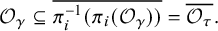
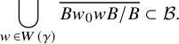
We can now state Brion’s formula [Reference BrionBri01, Theorem 6].
Theorem 2.11 (Brion).
Let $\gamma \in \mathbf {Clan}_{p,q}$
. The K-orbit closure
$\gamma \in \mathbf {Clan}_{p,q}$
. The K-orbit closure $\overline {{{\mathcal O}}_\gamma }$
has rational singularities and admits a flat degeneration to the reduced subscheme
$\overline {{{\mathcal O}}_\gamma }$
has rational singularities and admits a flat degeneration to the reduced subscheme
 $$ \begin{align*} \bigcup_{w\in W(\gamma) } \overline{Bw_0 w B/B} \subset \mathcal{B}. \end{align*} $$
In particular, we have
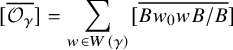 $$ \begin{align} [\overline{{{\mathcal O}}_\gamma}] = \sum_{w\in W(\gamma) } [\overline{Bw_0 w B/B}] \end{align} $$
in the integral cohomology ring of $\mathcal {B}$
.
$\mathcal {B}$
.
Remark 2.12. Let us denote by $\mathcal {B}(G/K)$
the set of all B-orbit closures in a spherical homogeneous space
$\mathcal {B}(G/K)$
the set of all B-orbit closures in a spherical homogeneous space $G/K$
, where G is a complex connected reductive algebraic group, and K is a spherical subgroup of G. (As usual, T, B and W stand for a maximal torus in G, a Borel subgroup containing T in G, and the Weyl group of G, respectively.) For
$G/K$
, where G is a complex connected reductive algebraic group, and K is a spherical subgroup of G. (As usual, T, B and W stand for a maximal torus in G, a Borel subgroup containing T in G, and the Weyl group of G, respectively.) For $Y\in \mathcal {B}(G/K)$
, the W-set of Y consists of
$Y\in \mathcal {B}(G/K)$
, the W-set of Y consists of $w\in W$
such that the natural quotient morphism
$w\in W$
such that the natural quotient morphism $\pi _{Y,w} : \overline {BwB}\times _B Y\to G/K$
is surjective and generically finite. It turns out that, by [Reference BrionBri01, Lemma 5], this definition is equivalent to a generalization of our Definition 2.10 to the setup of spherical homogeneous spaces.
$\pi _{Y,w} : \overline {BwB}\times _B Y\to G/K$
is surjective and generically finite. It turns out that, by [Reference BrionBri01, Lemma 5], this definition is equivalent to a generalization of our Definition 2.10 to the setup of spherical homogeneous spaces.
Let $d(Y,w)$
denote the degree of
$d(Y,w)$
denote the degree of $\pi _{Y,w}$
. It turns out that this number is always a power of 2, [Reference BrionBri01, Lemma 5 (iii)]. The real geometric usefulness of this integer is explained by Brion in [Reference BrionBri01, Theorem 6]. In particular, the cohomology class corresponding to Y in
$\pi _{Y,w}$
. It turns out that this number is always a power of 2, [Reference BrionBri01, Lemma 5 (iii)]. The real geometric usefulness of this integer is explained by Brion in [Reference BrionBri01, Theorem 6]. In particular, the cohomology class corresponding to Y in $H^*(G/B,{\mathbb {Z}})$
is given by
$H^*(G/B,{\mathbb {Z}})$
is given by
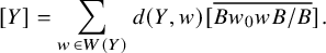 $$\begin{align*}[Y] = \sum_{w\in W(Y)} d(Y,w)[\overline{Bw_0 wB/B}]. \end{align*}$$
In our special case, where $K=GL_p({\mathbb {C}})\times GL_q({\mathbb {C}})$
, the work of Vust [Reference VustVus90] implies that each of these degrees is equal to
$K=GL_p({\mathbb {C}})\times GL_q({\mathbb {C}})$
, the work of Vust [Reference VustVus90] implies that each of these degrees is equal to $1$
, implying our identity (13). It also implies the vanishing of all higher cohomology spaces for the restrictions of effective line bundles from
$1$
, implying our identity (13). It also implies the vanishing of all higher cohomology spaces for the restrictions of effective line bundles from $G/B$
to Y.
$G/B$
to Y.
We now recall a combinatorial description for the weak order on $\mathbf {Clan}_{p,q}$
used in the work of the first author, Joyce and Wyser [Reference Can, Joyce and WyserCJW16]. This description is most easily stated in terms of charged matchings. A matching on
$\mathbf {Clan}_{p,q}$
used in the work of the first author, Joyce and Wyser [Reference Can, Joyce and WyserCJW16]. This description is most easily stated in terms of charged matchings. A matching on $[n]$
is a finite graph on the vertex set
$[n]$
is a finite graph on the vertex set $[n]$
such that each vertex is either isolated or adjacent to precisely one other vertex. A charged matching is a matching with an assignment of a
$[n]$
such that each vertex is either isolated or adjacent to precisely one other vertex. A charged matching is a matching with an assignment of a $+$
or
$+$
or $-$
charge to each isolated vertex.
$-$
charge to each isolated vertex.
The set of $(p,q)$
-clans is in bijection with the set of all charged matchings on
$(p,q)$
-clans is in bijection with the set of all charged matchings on $[n]$
having
$[n]$
having $p-q$
more
$p-q$
more $+$
’s than
$+$
’s than $-$
’s. Explicitly, we obtain a matching from a clan
$-$
’s. Explicitly, we obtain a matching from a clan $\gamma =c_1c_2\cdots c_n$
by connecting i and j by an arc whenever
$\gamma =c_1c_2\cdots c_n$
by connecting i and j by an arc whenever $c_i=c_j\in {\mathbb {Z}}_+$
and recording all signed entries as charges on isolated vertices. We identify the set of
$c_i=c_j\in {\mathbb {Z}}_+$
and recording all signed entries as charges on isolated vertices. We identify the set of $(p,q)$
-clans with charged matchings throughout, but particularly in Section 4 below.
$(p,q)$
-clans with charged matchings throughout, but particularly in Section 4 below.
Example 2.13. The matching associated to the (5,3)-clan $\gamma =+1+-2+21$
appears in Figure 1.
$\gamma =+1+-2+21$
appears in Figure 1.
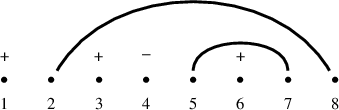
Figure 1 The matching for clan $\gamma =+1+-2+21$
.
$\gamma =+1+-2+21$
.
From [Reference Can, Joyce and WyserCJW16, Section 2.5], we get that the weak order on clans is the transitive closure of the covering relations
 $$\begin{align*}\gamma \xrightarrow{\; s_i \;} \gamma', \end{align*}$$
where we obtain $\gamma '$
from
$\gamma '$
from $\gamma $
according to one of the following moves on the corresponding charged matchings, each of which is illustrated in Figure 2 below.
$\gamma $
according to one of the following moves on the corresponding charged matchings, each of which is illustrated in Figure 2 below.
-
• Types IA1 and IA2: Switch the endpoint of a strand with an adjacent sign so as to lengthen the strand.
-
• Type IB: Create a crossing from two disjoint strands at consecutive vertices.
-
• Types IC1 and IC2: Create a nested pair of strands by uncrossing the ends of two crossing strands at consecutive vertices.
-
• Type II: Replace a pair of consecutive, opposite charges with a strand of length 1.
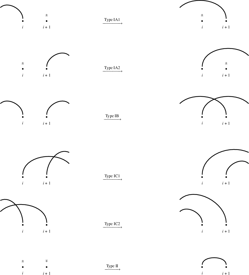
Figure 2 Cover relations of the weak order on $\mathbf {Clan}_{p,q}$
.
$\mathbf {Clan}_{p,q}$
.
An astute reader will note that [Reference Can, Joyce and WyserCJW16] actually studies the opposite weak order on $\mathbf {Clan}_{p,q}$
, so our Figure 2 reverses the covering relations as presented in Figure 2.5 of that reference.
$\mathbf {Clan}_{p,q}$
, so our Figure 2 reverses the covering relations as presented in Figure 2.5 of that reference.
3 Irreducible Hessenberg varieties
$\mathrm {Hess}(\mathsf {x}_{p,q},{\mathbf m})$

In this section, we classify all irreducible Hessenberg varieties of the form $\mathrm {Hess}(\mathsf {x}_{p,q},{\mathbf m})$
and prove Theorem 4 from the Introduction. To begin, we identify the K-orbits that are contained in
$\mathrm {Hess}(\mathsf {x}_{p,q},{\mathbf m})$
and prove Theorem 4 from the Introduction. To begin, we identify the K-orbits that are contained in $\mathrm {Hess}(\mathsf {x}_{p,q},{\mathbf m})$
.
$\mathrm {Hess}(\mathsf {x}_{p,q},{\mathbf m})$
.
Proposition 3.1. The K-orbit ${{\mathcal O}}_\gamma $
associated to the
${{\mathcal O}}_\gamma $
associated to the $(p,q)$
-clan
$(p,q)$
-clan $\gamma =c_1c_2\cdots c_n$
lies in
$\gamma =c_1c_2\cdots c_n$
lies in $\mathrm {Hess}(\mathsf {x}_{p,q},{\mathbf m})$
if and only if
$\mathrm {Hess}(\mathsf {x}_{p,q},{\mathbf m})$
if and only if $m_i \geq j$
whenever
$m_i \geq j$
whenever $c_i=c_j \in {\mathbb {Z}}_+$
with
$c_i=c_j \in {\mathbb {Z}}_+$
with $i<j$
.
$i<j$
.
Proof. It suffices to determine which clans $\gamma $
satisfy
$\gamma $
satisfy $V(\gamma )_\bullet \in \mathrm {Hess}(\mathsf {x}_{p,q},{\mathbf m})$
, where
$V(\gamma )_\bullet \in \mathrm {Hess}(\mathsf {x}_{p,q},{\mathbf m})$
, where $V(\gamma )$
is the flag representative of
$V(\gamma )$
is the flag representative of ${{\mathcal O}}_\gamma $
specified in Definition 2.1 above. We observe first that each
${{\mathcal O}}_\gamma $
specified in Definition 2.1 above. We observe first that each $e_i$
is an eigenvector for
$e_i$
is an eigenvector for $\mathsf {x}_{p,q}$
and that if
$\mathsf {x}_{p,q}$
and that if $v_i \in \{e_r+e_s,e_r-e_s\}$
with
$v_i \in \{e_r+e_s,e_r-e_s\}$
with $r \in [p]$
and
$r \in [p]$
and $p<s \leq n$
, then
$p<s \leq n$
, then ${\mathbb {C}}\{v_i,\mathsf {x}_{p,q} v_i\}={\mathbb {C}}\{e_r,e_s\}$
. Thus,
${\mathbb {C}}\{v_i,\mathsf {x}_{p,q} v_i\}={\mathbb {C}}\{e_r,e_s\}$
. Thus, $V(\gamma )_i+\mathsf {x}_{p,q} V(\gamma )_i$
is spanned by those standard basis vectors
$V(\gamma )_i+\mathsf {x}_{p,q} V(\gamma )_i$
is spanned by those standard basis vectors $e_k$
such that one of
$e_k$
such that one of
-
(A) there is some
$j \in [i]$
with
$v_j=e_k$
, or -
(B) there is some
$a \in [i]$
with
$v_a=e_r+e_s$
and
$k \in \{r,s\}$


holds. On the other hand, the standard basis vector $e_k$
is an element of
$e_k$
is an element of $V(\gamma )_{m_i}$
if and only if one of
$V(\gamma )_{m_i}$
if and only if one of
-
(A’) there is some
$j \in [m_i]$
with
$v_j=e_k$
, or -
(B’) there is some
$b \in [m_i]$
with
$v_b=e_r-e_s$
and
$k \in \{r,s\}$


holds. Indeed, if there is no $j \in [m_i]$
with
$j \in [m_i]$
with $v_j=e_k$
, then
$v_j=e_k$
, then $e_k \in V(\gamma )_{m_i}$
if and only if there are
$e_k \in V(\gamma )_{m_i}$
if and only if there are $a,b \in [m_i]$
with
$a,b \in [m_i]$
with $v_a=e_r+e_s$
,
$v_a=e_r+e_s$
, $v_b=e_r-e_s$
and
$v_b=e_r-e_s$
and $k \in \{r,s\}$
. In this case,
$k \in \{r,s\}$
. In this case, $a<b$
and
$a<b$
and $c_a=c_b$
by definition of the flag
$c_a=c_b$
by definition of the flag $V(\gamma )_\bullet $
.
$V(\gamma )_\bullet $
.
For each i, we have $V(\gamma )_i\leq V(\gamma )_{m_i}$
since
$V(\gamma )_i\leq V(\gamma )_{m_i}$
since $m_i\geq i$
. Thus,
$m_i\geq i$
. Thus, $V(\gamma )\in \mathrm {Hess}(\mathsf {x}_{p,q},{\mathbf m})$
if and only if
$V(\gamma )\in \mathrm {Hess}(\mathsf {x}_{p,q},{\mathbf m})$
if and only if $V(\gamma )_i+\mathsf {x}_{p,q}V(\gamma )_i \leq V(\gamma )_{m_i}$
for all i. Suppose
$V(\gamma )_i+\mathsf {x}_{p,q}V(\gamma )_i \leq V(\gamma )_{m_i}$
for all i. Suppose $e_k\in V(\gamma )_i +\mathsf {x}_{p,q}V(\gamma _i)$
, so we are in either Case (A) or Case (B) from above. In Case (A), the vector
$e_k\in V(\gamma )_i +\mathsf {x}_{p,q}V(\gamma _i)$
, so we are in either Case (A) or Case (B) from above. In Case (A), the vector $e_k$
is also an element of
$e_k$
is also an element of $V(\gamma )_{m_i}$
by (A’) since
$V(\gamma )_{m_i}$
by (A’) since $i\leq m_i$
.
$i\leq m_i$
.
In Case (B), there exists $a\in [i]$
such that
$a\in [i]$
such that $v_a=e_r+e_s$
, and we have
$v_a=e_r+e_s$
, and we have ${\mathbb {C}}\{e_r,e_s\}\leq V(\gamma )_i +\mathsf {x}_{p,q}V(\gamma _i)$
with
${\mathbb {C}}\{e_r,e_s\}\leq V(\gamma )_i +\mathsf {x}_{p,q}V(\gamma _i)$
with $k\in \{r,s\}$
. By definition of the flag
$k\in \{r,s\}$
. By definition of the flag $V(\gamma )$
, there exists some
$V(\gamma )$
, there exists some $b>a$
such that
$b>a$
such that $c_a=c_b$
and
$c_a=c_b$
and $v_b= e_r-e_s$
. By (B’),
$v_b= e_r-e_s$
. By (B’), ${\mathbb {C}}\{e_r,e_s\}\leq V(\gamma )_{m_i}$
if and only if
${\mathbb {C}}\{e_r,e_s\}\leq V(\gamma )_{m_i}$
if and only if $b\in [m_i]$
– that is, if
$b\in [m_i]$
– that is, if $b\leq m_i$
. The proposition follows.
$b\leq m_i$
. The proposition follows.
As any $\mathrm {Hess}(\mathsf {x}_{p,q},{\mathbf m})$
is a union of K-orbits, the next proposition follows immediately from the definitions.
$\mathrm {Hess}(\mathsf {x}_{p,q},{\mathbf m})$
is a union of K-orbits, the next proposition follows immediately from the definitions.
Proposition 3.2. The Hessenberg variety $\mathrm {Hess}(\mathsf {x}_{p,q},{\mathbf m})$
is irreducible if and only if, among the clans corresponding to K-orbits contained in
$\mathrm {Hess}(\mathsf {x}_{p,q},{\mathbf m})$
is irreducible if and only if, among the clans corresponding to K-orbits contained in $\mathrm {Hess}(\mathsf {x}_{p,q}, {\mathbf m})$
, there is a unique maximal one with respect to the inclusion order.
$\mathrm {Hess}(\mathsf {x}_{p,q}, {\mathbf m})$
, there is a unique maximal one with respect to the inclusion order.
Let us specify two particular clans $\sigma $
and
$\sigma $
and $\tau $
in
$\tau $
in $\mathbf {Clan}_{p,q}$
by
$\mathbf {Clan}_{p,q}$
by
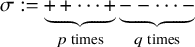 $$\begin{align*}\sigma:= \underbrace{++ \cdots +}_{p \text{ times}}\underbrace{--\cdots -}_{q \text{ times}} \end{align*}$$
and
 $$\begin{align*}\tau:= \underbrace{-- \cdots -}_{q \text{ times}}\underbrace{++\cdots +}_{p \text{ times}}. \end{align*}$$
Observe that $\sigma (i;-)=0$
for
$\sigma (i;-)=0$
for $i \leq p$
and
$i \leq p$
and $\tau (i;+)=0$
for
$\tau (i;+)=0$
for $i \leq q$
. Under our assumption that
$i \leq q$
. Under our assumption that $p \geq q$
, the next claim follows.
$p \geq q$
, the next claim follows.
Lemma 3.3. If $\gamma =c_1c_2\cdots c_n\in \mathbf {Clan}_{p,q}$
such that
$\gamma =c_1c_2\cdots c_n\in \mathbf {Clan}_{p,q}$
such that $\sigma \leq \gamma $
and
$\sigma \leq \gamma $
and $\tau \leq \gamma $
, then all of
$\tau \leq \gamma $
, then all of
-
(a)
$c_i=i$
for each
$i \in [q]$
, -
(b)
$c_i=+$
for
$q<i \leq p$
, and -
(c)
$\{c_i \mid p<i \leq p+q\}=[q]$


hold. In particular, if $\overline {{{\mathcal O}}_\gamma }=\mathrm {Hess}(\mathsf {x}_{p,q},{\mathbf m})$
for some Hessenberg vector
$\overline {{{\mathcal O}}_\gamma }=\mathrm {Hess}(\mathsf {x}_{p,q},{\mathbf m})$
for some Hessenberg vector ${\mathbf m}$
, then
${\mathbf m}$
, then $\gamma $
satisfies all three conditions.
$\gamma $
satisfies all three conditions.
Proof. As each of ${{\mathcal O}}_\sigma $
and
${{\mathcal O}}_\sigma $
and ${{\mathcal O}}_\tau $
lies in
${{\mathcal O}}_\tau $
lies in $\overline {{{\mathcal O}}_\gamma }$
, we have
$\overline {{{\mathcal O}}_\gamma }$
, we have
-
•
$\gamma (i;-) \leq \sigma (i;-)=0$
for
$i \leq p$
and -
•
$\gamma (i;+) \leq \tau (i;+)=0$
for
$i \leq q$


by Theorem 2.7. These conditions imply that $\gamma $
cannot contain any signs or pairs of positive integers within the first q entries and cannot contain any minus signs or pairs of positive integers within the first p entries. Since
$\gamma $
cannot contain any signs or pairs of positive integers within the first q entries and cannot contain any minus signs or pairs of positive integers within the first p entries. Since $\gamma $
contains at most q natural number pairs, conditions (a) and (b) now follow. Condition (c) follows from (a) and (b) and the fact that
$\gamma $
contains at most q natural number pairs, conditions (a) and (b) now follow. Condition (c) follows from (a) and (b) and the fact that $\gamma $
is a clan. The last statement of the lemma follows immediately, as both
$\gamma $
is a clan. The last statement of the lemma follows immediately, as both ${{\mathcal O}}_\sigma $
and
${{\mathcal O}}_\sigma $
and ${{\mathcal O}}_\tau $
lie in
${{\mathcal O}}_\tau $
lie in $\mathrm {Hess}(\mathsf {x}_{p,q},{\mathbf m})$
for every Hessenberg vector
$\mathrm {Hess}(\mathsf {x}_{p,q},{\mathbf m})$
for every Hessenberg vector ${\mathbf m}$
by Proposition 3.1.
${\mathbf m}$
by Proposition 3.1.
We can rewrite condition (c) from Lemma 3.3 as
-
(c’) there is some
$w \in {\mathbf {S}}_q$
such that
$c_{p+i}=w(i)$
for each
$i \in [q]$
.


Given a clan $\gamma $
satisfying (a),(b) and (c’), we write
$\gamma $
satisfying (a),(b) and (c’), we write $\gamma _w$
for
$\gamma _w$
for $\gamma $
. Thus, for each
$\gamma $
. Thus, for each $w\in {\mathbf {S}}_q$
, we obtain a unique clan
$w\in {\mathbf {S}}_q$
, we obtain a unique clan $\gamma _w=c_1^wc_2^w \cdots c_n^w$
defined by
$\gamma _w=c_1^wc_2^w \cdots c_n^w$
defined by
-
•
$c_i^w= +$
for all
$q<i \leq p$
, and -
•
$c_i^w=c_{p+w^{-1}(i)}^w=i$
for all
$i\in [q]$
.


Note that $\gamma _0=\gamma _{y_0}$
where
$\gamma _0=\gamma _{y_0}$
where $y_0$
is the longest permutation in
$y_0$
is the longest permutation in ${\mathbf {S}}_q$
. In fact, the collection of all such
${\mathbf {S}}_q$
. In fact, the collection of all such $(p,q)$
-clans forms is precisely the inclusion-interval
$(p,q)$
-clans forms is precisely the inclusion-interval $[\gamma _e, \gamma _0]$
in
$[\gamma _e, \gamma _0]$
in $\mathbf {Clan}_{p,q}$
.
$\mathbf {Clan}_{p,q}$
.
Lemma 3.4. Let $\gamma _e = 12\cdots q + \cdots +12\cdots q$
be the clan corresponding to the identity in
$\gamma _e = 12\cdots q + \cdots +12\cdots q$
be the clan corresponding to the identity in ${\mathbf {S}}_q$
. If
${\mathbf {S}}_q$
. If $\gamma _e \leq \gamma $
, then
$\gamma _e \leq \gamma $
, then $\gamma =\gamma _w$
for some
$\gamma =\gamma _w$
for some $w\in {\mathbf {S}}_q$
. In particular,
$w\in {\mathbf {S}}_q$
. In particular, $\gamma _w(i;+)=\gamma _0(i;+)$
and
$\gamma _w(i;+)=\gamma _0(i;+)$
and $\gamma _w(i;-)=\gamma _0(i;-)$
for all i, and
$\gamma _w(i;-)=\gamma _0(i;-)$
for all i, and $\gamma _w(i,j) = \gamma _0(i,j)$
whenever
$\gamma _w(i,j) = \gamma _0(i,j)$
whenever $i, j \in [p]$
or
$i, j \in [p]$
or $i, j \in \{p+1, \ldots , n\}$
.
$i, j \in \{p+1, \ldots , n\}$
.
Proof. We observe that both $\sigma \leq \gamma _e$
and
$\sigma \leq \gamma _e$
and $\tau \leq \gamma _e$
. Thus,
$\tau \leq \gamma _e$
. Thus, $\gamma $
satisfies each of the conditions (a), (b) and (c’) by Lemma 3.3, and the first assertion of the lemma is proved. To prove the second, we observe that the equality of the various statistics holds in the case of
$\gamma $
satisfies each of the conditions (a), (b) and (c’) by Lemma 3.3, and the first assertion of the lemma is proved. To prove the second, we observe that the equality of the various statistics holds in the case of $w=e$
; cf. Example 2.8. The general case now follows since
$w=e$
; cf. Example 2.8. The general case now follows since $\gamma _0(i;-)\leq \gamma _w(i;-)\leq \gamma _e(i;-)$
,
$\gamma _0(i;-)\leq \gamma _w(i;-)\leq \gamma _e(i;-)$
, $\gamma _0(i;+)\leq \gamma _w(i;-)\leq \gamma _e(i;+)$
, and
$\gamma _0(i;+)\leq \gamma _w(i;-)\leq \gamma _e(i;+)$
, and $\gamma _e(i,j)\leq \gamma _w(i,j)\leq \gamma _0(i,j)$
by Theorem 2.7 in all cases.
$\gamma _e(i,j)\leq \gamma _w(i,j)\leq \gamma _0(i,j)$
by Theorem 2.7 in all cases.
The inclusion order on the clans in the interval $[\gamma _e, \gamma _0]$
is greatly simplified. Indeed, the only case in which the statistics appearing in Theorem 2.7 can differ is when considering
$[\gamma _e, \gamma _0]$
is greatly simplified. Indeed, the only case in which the statistics appearing in Theorem 2.7 can differ is when considering $\gamma _w(i,j)$
with
$\gamma _w(i,j)$
with $i\in [q]$
and
$i\in [q]$
and $j\in \{p+1,p+2,\ldots , n\}$
. In that situation, we obtain the following.
$j\in \{p+1,p+2,\ldots , n\}$
. In that situation, we obtain the following.
Lemma 3.5. For all $w\in {\mathbf {S}}_q$
and all
$w\in {\mathbf {S}}_q$
and all $i \in [q], j \in \{p+1, \ldots , n\}$
,
$i \in [q], j \in \{p+1, \ldots , n\}$
,
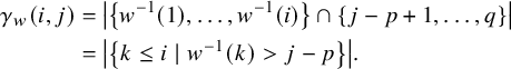 $$ \begin{align*}\begin{aligned} \gamma_w(i, j) & =\left|\left\{w^{-1}(1), \ldots, w^{-1}(i)\right\} \cap\{j-p+1, \ldots, q\}\right| \\ & =\left|\left\{k \leq i \mid w^{-1}(k)>j-p\right\}\right|. \end{aligned} \end{align*} $$
Proof. We have a pair $s<t$
such that
$s<t$
such that $s \leq i<j<t$
and
$s \leq i<j<t$
and $c_s^w=c_t^w$
if and only if
$c_s^w=c_t^w$
if and only if $t=w^{-1}(s)+p$
by definition of
$t=w^{-1}(s)+p$
by definition of $\gamma _w$
.
$\gamma _w$
.
Example 3.6. Consider $(5,3)$
-clans
$(5,3)$
-clans $\gamma _w = 123++213$
and
$\gamma _w = 123++213$
and $\gamma _{w'} = 123++132$
. For the clan
$\gamma _{w'} = 123++132$
. For the clan $\gamma _w$
,
$\gamma _w$
, $w(1)=2, w(2)=1,$
and
$w(1)=2, w(2)=1,$
and $w(3)=3$
, while for
$w(3)=3$
, while for $\gamma _{w'}$
, we have
$\gamma _{w'}$
, we have $w'(1)=1, w'(2)=3,$
and
$w'(1)=1, w'(2)=3,$
and $w'(3)=2$
. The definition of
$w'(3)=2$
. The definition of $\gamma (i;j)$
and straightforward calculation give us that
$\gamma (i;j)$
and straightforward calculation give us that
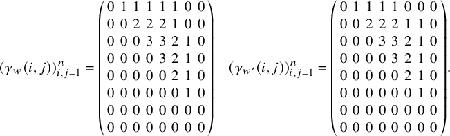 $$ \begin{align*}(\gamma_w(i,j))_{i,j=1}^n=\left( \begin{array}{cccccccc} 0 & 1 & 1 & 1 & 1 & 1 & 0 & 0 \\ 0 & 0 & 2 & 2 & 2 & 1 & 0 & 0 \\ 0 & 0 & 0 & 3 & 3 & 2 & 1 & 0 \\ 0 & 0 & 0 & 0 & 3 & 2 & 1 & 0 \\ 0 & 0 & 0 & 0 & 0 & 2 & 1 & 0 \\ 0 & 0 & 0 & 0 & 0 & 0 & 1 & 0 \\ 0 & 0 & 0 & 0 & 0 & 0 & 0 & 0 \\ 0 & 0 & 0 & 0 & 0 & 0 & 0 & 0 \end{array} \right) \quad (\gamma_{w'}(i,j))_{i,j=1}^n=\left( \begin{array}{cccccccc} 0 & 1 & 1 & 1 & 1 & 0 & 0 & 0 \\ 0 & 0 & 2 & 2 & 2 & 1 & 1 & 0 \\ 0 & 0 & 0 & 3 & 3 & 2 & 1 & 0 \\ 0 & 0 & 0 & 0 & 3 & 2 & 1 & 0 \\ 0 & 0 & 0 & 0 & 0 & 2 & 1 & 0 \\ 0 & 0 & 0 & 0 & 0 & 0 & 1 & 0 \\ 0 & 0 & 0 & 0 & 0 & 0 & 0 & 0 \\ 0 & 0 & 0 & 0 & 0 & 0 & 0 & 0 \end{array} \right). \end{align*} $$
Moreover, it also follows from Lemma 3.5 that
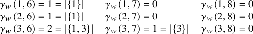 $$\begin{align*}\begin{array}{lclcl} \gamma_w(1,6)=1=|\{1\}| &\;\;& \gamma_w(1,7)=0 &\;\;& \gamma_w(1,8)=0 \\ \gamma_w(2,6)=1=|\{1\}| &\;\;& \gamma_w(2,7)=0 &\;\;& \gamma_w(2,8)=0 \\ \gamma_w(3,6)=2=|\{1, 3\}| &\;\;& \gamma_w(3,7)=1=|\{3\}| &\;\;& \gamma_w(3,8)=0 \end{array}\end{align*}$$
and,
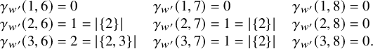 $$\begin{align*}\begin{array}{lclcl} \gamma_{w'}(1,6)=0 &\;\;& \gamma_{w'}(1,7)=0 &\;\;& \gamma_{w'}(1,8)=0 \\ \gamma_{w'}(2,6)=1=|\{2\}| &\;\;& \gamma_{w'}(2,7)=1=|\{2\}| &\;\;& \gamma_{w'}(2,8)=0 \\ \gamma_{w'}(3,6)=2=|\{2, 3\}| &\;\;& \gamma_{w'}(3,7)=1=|\{2\}| &\;\;& \gamma_{w'}(3,8)=0. \end{array}\end{align*}$$
Therefore, the statistics from Theorem 2.7 only differ for these clans when $(i,j)$
is either
$(i,j)$
is either $(1,6)$
or
$(1,6)$
or $(2,7)$
.
$(2,7)$
.
Our work above tells us that if $\mathrm {Hess}(\mathsf {x}_{p,q},{\mathbf m})$
is the closure of a single K-orbit, then that K-orbit is equal to
$\mathrm {Hess}(\mathsf {x}_{p,q},{\mathbf m})$
is the closure of a single K-orbit, then that K-orbit is equal to ${{\mathcal O}}_{\gamma _w}$
for some
${{\mathcal O}}_{\gamma _w}$
for some $w\in {\mathbf {S}}_q$
.
$w\in {\mathbf {S}}_q$
.
Corollary 3.7. Let ${\mathbf m}=(m_1,\ldots ,m_n)$
be a Hessenberg vector. If there is some clan
${\mathbf m}=(m_1,\ldots ,m_n)$
be a Hessenberg vector. If there is some clan $\gamma $
such that
$\gamma $
such that $\mathrm {Hess}(\mathsf {x}_{p,q},{\mathbf m})=\overline {{{\mathcal O}}_\gamma }$
, then
$\mathrm {Hess}(\mathsf {x}_{p,q},{\mathbf m})=\overline {{{\mathcal O}}_\gamma }$
, then $\gamma =\gamma _w$
for some
$\gamma =\gamma _w$
for some $w \in {\mathbf {S}}_q$
. Furthermore,
$w \in {\mathbf {S}}_q$
. Furthermore, $(m_1-p,m_2-p,\ldots ,m_q-p)$
is a Hessenberg vector of length q and
$(m_1-p,m_2-p,\ldots ,m_q-p)$
is a Hessenberg vector of length q and $m_i=n$
for all
$m_i=n$
for all $i\geq q$
.
$i\geq q$
.
Proof. It follows immediately from Lemma 3.3 that $\gamma =\gamma _w$
for some
$\gamma =\gamma _w$
for some $w \in {\mathbf {S}}_q$
. By Proposition 3.1, for each
$w \in {\mathbf {S}}_q$
. By Proposition 3.1, for each $i \in [q]$
, we have
$i \in [q]$
, we have $m_i \geq p+w^{-1}(i)$
. Thus, for each
$m_i \geq p+w^{-1}(i)$
. Thus, for each $i\in [q]$
,
$i\in [q]$
,
 $$\begin{align*}p+w^{-1}(i)\leq m_i \leq p+q \Leftrightarrow w^{-1}(i) \leq m_i -p \leq q. \end{align*}$$
It follows that $(m_1-p,m_2-p,\ldots ,m_q-p)$
is a sequence of positive integers satisfying
$(m_1-p,m_2-p,\ldots ,m_q-p)$
is a sequence of positive integers satisfying $m_i-p \leq q$
; it is also weakly increasing since
$m_i-p \leq q$
; it is also weakly increasing since ${\mathbf m}$
is. Moreover, for each
${\mathbf m}$
is. Moreover, for each $i \in [q]$
,
$i \in [q]$
,
 $$ \begin{align*}m_i-p \geq \max\{w^{-1}(j) \mid j \leq i\} \geq i. \end{align*} $$
This concludes the proof.
It follows from Corollary 3.7 that there are at most $\mathsf {Cat}_q=\frac {1}{q+1}{{2q} \choose {q}}$
Hessenberg vectors
$\mathsf {Cat}_q=\frac {1}{q+1}{{2q} \choose {q}}$
Hessenberg vectors ${\mathbf m}$
of length
${\mathbf m}$
of length $p+q$
such that
$p+q$
such that $\mathrm {Hess}(\mathsf {x}_{p,q},{\mathbf m})$
is a K-orbit closure as there are
$\mathrm {Hess}(\mathsf {x}_{p,q},{\mathbf m})$
is a K-orbit closure as there are $\mathsf {Cat}_q$
Hessenberg vectors of length q. We aim to show that there are exactly
$\mathsf {Cat}_q$
Hessenberg vectors of length q. We aim to show that there are exactly $\mathsf {Cat}_q$
such
$\mathsf {Cat}_q$
such ${\mathbf m}$
, and classify the set of
${\mathbf m}$
, and classify the set of $\mathsf {Cat}_q$
clans
$\mathsf {Cat}_q$
clans $\gamma $
such that
$\gamma $
such that $\mathrm {Hess}(\mathsf {x}_{p,q},{\mathbf m})=\overline {{{\mathcal O}}_\gamma }$
.
$\mathrm {Hess}(\mathsf {x}_{p,q},{\mathbf m})=\overline {{{\mathcal O}}_\gamma }$
.
Lemma 3.8. Assume $u \in {\mathbf {S}}_q$
and
$u \in {\mathbf {S}}_q$
and ${\mathbf m}$
is a Hessenberg vector such that
${\mathbf m}$
is a Hessenberg vector such that ${{\mathcal O}}_{\gamma _u} \subseteq \mathrm {Hess}(\mathsf {x}_{p,q},{\mathbf m})$
. If there exist
${{\mathcal O}}_{\gamma _u} \subseteq \mathrm {Hess}(\mathsf {x}_{p,q},{\mathbf m})$
. If there exist $i<j<k$
such that
$i<j<k$
such that $u^{-1}(i)>u^{-1}(k)>u^{-1}(j)$
, then there is some
$u^{-1}(i)>u^{-1}(k)>u^{-1}(j)$
, then there is some $w \in {\mathbf {S}}_q$
such that
$w \in {\mathbf {S}}_q$
such that $\gamma _u \leq \gamma _w$
and
$\gamma _u \leq \gamma _w$
and ${{\mathcal O}}_{\gamma _w} \subseteq \mathrm {Hess}(\mathsf {x}_{p,q},{\mathbf m})$
.
${{\mathcal O}}_{\gamma _w} \subseteq \mathrm {Hess}(\mathsf {x}_{p,q},{\mathbf m})$
.
Proof. Let w be obtained from u by switching j and k. Direct examination shows that for all $a,b \in [n]$
, all of
$a,b \in [n]$
, all of $\gamma _w(a;+) \leq \gamma _u(a;+)$
,
$\gamma _w(a;+) \leq \gamma _u(a;+)$
, $\gamma _w(a;-) \leq \gamma _u(a;-)$
and
$\gamma _w(a;-) \leq \gamma _u(a;-)$
and $\gamma _w(a,b) \geq \gamma _u(a,b)$
hold. Thus,
$\gamma _w(a,b) \geq \gamma _u(a,b)$
hold. Thus, $\gamma _u \leq \gamma _w$
by Theorem 2.7. Assume for contradiction that there exist
$\gamma _u \leq \gamma _w$
by Theorem 2.7. Assume for contradiction that there exist $a,b \in [n]$
with
$a,b \in [n]$
with $a<b$
and
$a<b$
and $s \in [q]$
such that
$s \in [q]$
such that $c^w_a=c^w_b=s$
and
$c^w_a=c^w_b=s$
and $b>m_a$
. By the definition of the clan
$b>m_a$
. By the definition of the clan $\gamma _w$
,
$\gamma _w$
, $a \in [q]$
and
$a \in [q]$
and $b=p+w^{-1}(a)$
. Since
$b=p+w^{-1}(a)$
. Since ${{\mathcal O}}_{\gamma _u} \subseteq \mathrm {Hess}(\mathsf {x}_{p,q},{\mathbf m})$
, it must be that
${{\mathcal O}}_{\gamma _u} \subseteq \mathrm {Hess}(\mathsf {x}_{p,q},{\mathbf m})$
, it must be that $a \in \{j,k\}$
and so
$a \in \{j,k\}$
and so $b \in \{p+w(j),p+w(k)\}$
. However,
$b \in \{p+w(j),p+w(k)\}$
. However,
 $$ \begin{align*}m_a>m_i \geq p+u^{-1}(i)=p+w^{-1}(i)>p+\max\{w^{-1}(j),w^{-1}(k)\} \geq b, \end{align*} $$
giving the desired contradiction.
Corollary 3.9. Let $w \in {\mathbf {S}}_q$
. If there is some Hessenberg vector
$w \in {\mathbf {S}}_q$
. If there is some Hessenberg vector ${\mathbf m}$
such that
${\mathbf m}$
such that $\mathrm {Hess}(\mathsf {x}_{p,q},{\mathbf m})=\overline {{{\mathcal O}}_{\gamma _w}}$
, then
$\mathrm {Hess}(\mathsf {x}_{p,q},{\mathbf m})=\overline {{{\mathcal O}}_{\gamma _w}}$
, then $w^{-1}$
avoids the pattern
$w^{-1}$
avoids the pattern $312$
; hence, w avoids
$312$
; hence, w avoids $231$
.
$231$
.
There are $\mathsf {Cat}_q$
elements
$\mathsf {Cat}_q$
elements $w \in {\mathbf {S}}_q$
avoiding
$w \in {\mathbf {S}}_q$
avoiding $231$
. Let
$231$
. Let
 $$\begin{align*}\mathbf{Clan}_{p,q}^{231}:= \{ \gamma_w\mid w\in {\mathbf{S}}_q,\, w \text{ avoids } 231 \}. \end{align*}$$
We prove below that this set of clans parameterizes irreducible semisimple Hessenberg varieties of the form $\mathrm {Hess}(\mathsf {x}_{p,q}, {\mathbf m})$
. For each
$\mathrm {Hess}(\mathsf {x}_{p,q}, {\mathbf m})$
. For each $w\in {\mathbf {S}}_q$
avoiding the pattern
$w\in {\mathbf {S}}_q$
avoiding the pattern $231$
, define a length
$231$
, define a length $n=p+q$
Hessenberg vector
$n=p+q$
Hessenberg vector ${\mathbf m}(w)$
by
${\mathbf m}(w)$
by
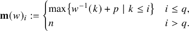 $$ \begin{align*}{\mathbf m}(w)_i:=\begin{cases}\max \left\{w^{-1}(k)+p \mid k \leq i\right\} & i \leq q, \\ n & i>q .\end{cases} \end{align*} $$
Example 3.10. Consider the $(5,3)$
-clan
$(5,3)$
-clan $\gamma _w = 123++213$
from
$\gamma _w = 123++213$
from $\mathbf {Clan}_{p,q}^{231}$
. Then for
$\mathbf {Clan}_{p,q}^{231}$
. Then for $i \leq 3$
, we have
$i \leq 3$
, we have
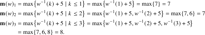 $$ \begin{align*}\begin{aligned} {\mathbf m}(w)_1 &= \max \left\{w^{-1}(k)+5 \mid k \leq 1\right\} = \max \left\{w^{-1}(1)+5\right\} = \max\{7\} = 7 \\ {\mathbf m}(w)_2 &= \max \left\{w^{-1}(k)+5 \mid k \leq 2\right\} = \max \left\{w^{-1}(1)+5, w^{-1}(2)+5 \right\} = \max\{7,6\}= 7\\ {\mathbf m}(w)_3 &= \max \left\{w^{-1}(k)+5 \mid k \leq 3\right\} =\max \left\{w^{-1}(1)+5, w^{-1}(2)+5, w^{-1}(3)+5 \right\}\\ &= \max \left\{7, 6, 8\right\} =8. \end{aligned}\end{align*} $$
For all $i> 3$
,
$i> 3$
, ${\mathbf m}(w)_i = 8$
. Thus, the associated Hessenberg vector is
${\mathbf m}(w)_i = 8$
. Thus, the associated Hessenberg vector is
 $$\begin{align*}{\mathbf m}(w)= (7, 7, 8, 8, 8, 8, 8, 8). \end{align*}$$
Consider the $(5,3)$
-clan
$(5,3)$
-clan $\gamma _{w'} = 123++132$
from
$\gamma _{w'} = 123++132$
from $\mathbf {Clan}_{p,q}^{231}$
. Then for
$\mathbf {Clan}_{p,q}^{231}$
. Then for $i \leq 3$
, we have
$i \leq 3$
, we have
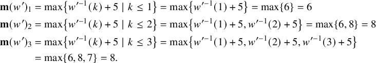 $$ \begin{align*}\begin{aligned} {\mathbf m}(w')_1 &= \max \left\{w^{\prime -1}(k)+5 \mid k \leq 1\right\} = \max \left\{w^{\prime -1}(1)+5\right\} = \max \left\{6\right\} = 6 \\ {\mathbf m}(w')_2 &= \max \left\{w^{\prime -1}(k)+5 \mid k \leq 2\right\} = \max \left\{w^{\prime -1}(1)+5, w^{\prime -1}(2)+5 \right\}= \max \left\{6, 8\right\} = 8\\ {\mathbf m}(w')_3 &= \max \left\{w^{\prime -1}(k)+5 \mid k \leq 3\right\} =\max \left\{w^{\prime -1}(1)+5, w^{\prime -1}(2)+5, w^{\prime -1}(3)+5 \right\}\\ &= \max \left\{6, 8, 7\right\} =8. \end{aligned}\end{align*} $$
For all $i> 3$
,
$i> 3$
, ${\mathbf m}(w')_i = 8$
. Thus, the associated Hessenberg vector is
${\mathbf m}(w')_i = 8$
. Thus, the associated Hessenberg vector is
 $$\begin{align*}{\mathbf m}(w')= (6, 8, 8, 8, 8, 8, 8, 8). \end{align*}$$
We can now state the main theorem of this section.
Theorem 3.11. For each $w\in {\mathbf {S}}_q$
avoiding the pattern
$w\in {\mathbf {S}}_q$
avoiding the pattern $231$
, the Hessenberg variety
$231$
, the Hessenberg variety $\mathrm {Hess}(\mathsf {x}_{p,q},{\mathbf m}(w))$
is irreducible and equal to the closure of the K-orbit
$\mathrm {Hess}(\mathsf {x}_{p,q},{\mathbf m}(w))$
is irreducible and equal to the closure of the K-orbit ${{\mathcal O}}_{\gamma _w}$
. Furthermore, every irreducible Hessenberg variety defined using the semisimple matrix
${{\mathcal O}}_{\gamma _w}$
. Furthermore, every irreducible Hessenberg variety defined using the semisimple matrix $\mathsf {x}_{p,q}$
is of this form.
$\mathsf {x}_{p,q}$
is of this form.
Our proof of Theorem 3.11 requires the following technical lemma.
Lemma 3.12. Let $w\in {\mathbf {S}}_q$
be
$w\in {\mathbf {S}}_q$
be $231$
-free and
$231$
-free and ${\mathbf m}={\mathbf m}(w)$
the associated Hessenberg vector defined above. Let
${\mathbf m}={\mathbf m}(w)$
the associated Hessenberg vector defined above. Let $i \in [q]$
such that
$i \in [q]$
such that $w^{-1}(i)+p< m_i$
. Then for all j with
$w^{-1}(i)+p< m_i$
. Then for all j with $w^{-1}(i)+p \leq j< m_i$
,
$w^{-1}(i)+p \leq j< m_i$
, $\gamma _w(i-1, j)= m_i-j$
.
$\gamma _w(i-1, j)= m_i-j$
.
Proof. By Lemma 3.5, $\gamma _w(i-1, j)=\left |\left \{k<i \mid w^{-1}(k)>j-p\right \}\right |$
. By definition of the Hessenberg vector
$\gamma _w(i-1, j)=\left |\left \{k<i \mid w^{-1}(k)>j-p\right \}\right |$
. By definition of the Hessenberg vector ${\mathbf m}$
, there exists
${\mathbf m}$
, there exists $a<i$
such that
$a<i$
such that $m_i=w^{-1}(a)+p$
. Our assumptions imply that
$m_i=w^{-1}(a)+p$
. Our assumptions imply that
 $$ \begin{align*}j<m_i=w^{-1}(a)+p \Rightarrow j-p<w^{-1}(a)\quad \text{and} \quad w^{-1}(i)<w^{-1}(a). \end{align*} $$
Let $k \in \{1,2, \ldots , q\}$
such that
$k \in \{1,2, \ldots , q\}$
such that $j-p<w^{-1}(k) \leq w^{-1}(a)$
. Note that
$j-p<w^{-1}(k) \leq w^{-1}(a)$
. Note that $j-p<w^{-1}(k)$
implies
$j-p<w^{-1}(k)$
implies $w^{-1}(i)<w^{-1}(k)$
and
$w^{-1}(i)<w^{-1}(k)$
and $k \neq i$
.
$k \neq i$
.
If $k>i$
, then
$k>i$
, then $w^{-1}(k)<w^{-1}(a) $
and
$w^{-1}(k)<w^{-1}(a) $
and $w^{-1}$
contains
$w^{-1}$
contains $w^{-1}(a) w^{-1}(i) w^{-1}(k)$
as a subsequence, contradicting the fact that
$w^{-1}(a) w^{-1}(i) w^{-1}(k)$
as a subsequence, contradicting the fact that $w^{-1}$
is
$w^{-1}$
is $312$
-free. Thus, we must have
$312$
-free. Thus, we must have $k<i$
. This shows that
$k<i$
. This shows that
 $$ \begin{align*}\left\{k \in[q] \mid {j-p}<w^{-1}(k) \leq w^{-1}(a)\right\} \subseteq\left\{k<i \mid w^{-1}(k)>j-p\right\}. \end{align*} $$
The sets are actually equal, since
 $$ \begin{align*}w^{-1}(a)=\max \left\{w^{-1}(1), \ldots, w^{-1}(i)\right\}.\end{align*} $$
We conclude $\gamma _w(i-1, j)=w^{-1}(a)-(j-p)=m_i-j$
, as desired.
$\gamma _w(i-1, j)=w^{-1}(a)-(j-p)=m_i-j$
, as desired.
Proof of Theorem 3.11.
By Proposition 3.2, Corollary 3.7 and Corollary 3.9, every irreducible Hessenberg variety defined using $\mathsf {x}_{p,q}$
is equal to
$\mathsf {x}_{p,q}$
is equal to $\overline {{{\mathcal O}}_{\gamma _w}}$
for some
$\overline {{{\mathcal O}}_{\gamma _w}}$
for some $\gamma _w\in \mathbf {Clan}_{p,q}^{231}$
. To complete the proof, we show that
$\gamma _w\in \mathbf {Clan}_{p,q}^{231}$
. To complete the proof, we show that $\mathrm {Hess}(\mathsf {x}_{p,q}, {\mathbf m}(w)) = \overline {{{\mathcal O}}_{\gamma _w}}$
. It follows immediately from the definition of the Hessenberg vector
$\mathrm {Hess}(\mathsf {x}_{p,q}, {\mathbf m}(w)) = \overline {{{\mathcal O}}_{\gamma _w}}$
. It follows immediately from the definition of the Hessenberg vector ${\mathbf m}(w)$
and Proposition 3.1 that
${\mathbf m}(w)$
and Proposition 3.1 that ${{\mathcal O}}_{\gamma _w} \subset \mathrm {Hess}(\mathsf {x}_{p,q},{\mathbf m}(w))$
. It therefore suffices to show that if
${{\mathcal O}}_{\gamma _w} \subset \mathrm {Hess}(\mathsf {x}_{p,q},{\mathbf m}(w))$
. It therefore suffices to show that if ${{\mathcal O}}_\gamma \subset \mathrm {Hess}(\mathsf {x}_{p,q},{\mathbf m}(w))$
for some
${{\mathcal O}}_\gamma \subset \mathrm {Hess}(\mathsf {x}_{p,q},{\mathbf m}(w))$
for some $\gamma =c_1c_2\cdots c_n\in \mathbf {Clan}_{p,q}$
, then
$\gamma =c_1c_2\cdots c_n\in \mathbf {Clan}_{p,q}$
, then $\gamma \leq \gamma _w$
.
$\gamma \leq \gamma _w$
.
By Theorem 2.7 and Lemma 3.4, we must prove $\gamma (i, j) \leq \gamma _w(i, j)$
for all
$\gamma (i, j) \leq \gamma _w(i, j)$
for all $i \in [q]$
and
$i \in [q]$
and $j \in \{p+1, \ldots , n\}$
. Seeking a contradiction, suppose
$j \in \{p+1, \ldots , n\}$
. Seeking a contradiction, suppose $\gamma (i, j)>\gamma _w(i, j)$
. We may assume i is minimal with respect to this property. We write
$\gamma (i, j)>\gamma _w(i, j)$
. We may assume i is minimal with respect to this property. We write ${\mathbf m}={\mathbf m}(w)$
throughout to simplify notation.
${\mathbf m}={\mathbf m}(w)$
throughout to simplify notation.
Consider first the case $i=1$
. Note that
$i=1$
. Note that $\gamma (1, j), \gamma _w(1, j) \in \{0,1\}$
, so we must have
$\gamma (1, j), \gamma _w(1, j) \in \{0,1\}$
, so we must have $\gamma (1, j)=1$
and
$\gamma (1, j)=1$
and $\gamma _w(1, j)=0$
. The latter implies
$\gamma _w(1, j)=0$
. The latter implies $w^{-1}(1)+p \leq j$
by Lemma 3.5. On the other hand,
$w^{-1}(1)+p \leq j$
by Lemma 3.5. On the other hand, $\gamma (1, j)=1$
implies by Lemma 2.9 that there exists
$\gamma (1, j)=1$
implies by Lemma 2.9 that there exists $t>j$
such that
$t>j$
such that $c_1=c_t$
. Now
$c_1=c_t$
. Now $m_1=w^{-1}(1)+p<t$
, contradicting the assumption that
$m_1=w^{-1}(1)+p<t$
, contradicting the assumption that ${{\mathcal O}}_\gamma \subset \mathrm {Hess}(\mathsf {x}_{p, q}, {\mathbf m})$
.
${{\mathcal O}}_\gamma \subset \mathrm {Hess}(\mathsf {x}_{p, q}, {\mathbf m})$
.
Now, assume $i>1$
. We have both
$i>1$
. We have both $\gamma (i-1, j) \leq \gamma _w(i-1, j)$
and
$\gamma (i-1, j) \leq \gamma _w(i-1, j)$
and $\gamma (i, j)>\gamma _w(i, j)$
. By Lemma 2.9, this can only be the case if
$\gamma (i, j)>\gamma _w(i, j)$
. By Lemma 2.9, this can only be the case if
 $$ \begin{align} \gamma(i, j)-\gamma(i-1, j)=1, \end{align} $$
and
 $$ \begin{align} \gamma_w(i, j)-\gamma_w(i-1, j)=0. \end{align} $$
We may furthermore conclude that
 $$ \begin{align} \gamma(i-1, j)=\gamma_w(i-1, j) \end{align} $$
since otherwise, $\gamma (i-1, j)<\gamma _w(i-1, j)$
and
$\gamma (i-1, j)<\gamma _w(i-1, j)$
and
 $$ \begin{align*}\gamma(i, j)=\gamma(i-1, j)+1 \leq \gamma_w(i-1, j)=\gamma_w(i, j)_{,} \end{align*} $$
contradicting our assumption that $\gamma (i, j)>\gamma _w(i, j)$
.
$\gamma (i, j)>\gamma _w(i, j)$
.
By Lemma 2.9, equation (3) implies that there exists $t>j$
such that
$t>j$
such that $c_i=c_t$
. From equation (4), we get that
$c_i=c_t$
. From equation (4), we get that
 $$ \begin{align*} &\left|\left\{w^{-1}(1), \ldots, w^{-1}(i)\right\} \cap\{j-p+1, \ldots, q\}\right| = \\ & \quad \quad \quad\quad\quad\quad\quad \left|\left\{w^{-1}(1), \ldots, w^{-1}(i-1)\right\} \cap\{j-p+1, \ldots, q\}\right| \end{align*} $$
so $w^{-1}(i) \leq j-p$
, implying
$w^{-1}(i) \leq j-p$
, implying $w^{-1}(i)+p \leq j$
.
$w^{-1}(i)+p \leq j$
.
If $m_i=w^{-1}(i)+p$
, then we have
$m_i=w^{-1}(i)+p$
, then we have $m_i<t$
, a contradiction to
$m_i<t$
, a contradiction to ${{\mathcal O}}_\gamma \subset \mathrm {Hess}(\mathsf {x}_{p, q}, {\mathbf m})$
. We obtain the same contradiction if
${{\mathcal O}}_\gamma \subset \mathrm {Hess}(\mathsf {x}_{p, q}, {\mathbf m})$
. We obtain the same contradiction if $j \geq m_i$
so we may now assume both
$j \geq m_i$
so we may now assume both $m_i>w^{-1}(i)+p$
and
$m_i>w^{-1}(i)+p$
and $j<m_i$
. By Lemma 3.12 and equation (5),
$j<m_i$
. By Lemma 3.12 and equation (5), $\gamma (i-1, j)=m_i-j$
. This implies there are precisely
$\gamma (i-1, j)=m_i-j$
. This implies there are precisely $m_i-j$
pairs
$m_i-j$
pairs $(a<b)$
such that
$(a<b)$
such that $a \leq i-1<j<b$
and
$a \leq i-1<j<b$
and $c_a=c_b$
. As
$c_a=c_b$
. As ${{\mathcal O}}_{\gamma } \subseteq \mathrm {Hess}(\mathsf {x}_{p, q}, {\mathbf m})$
, we have
${{\mathcal O}}_{\gamma } \subseteq \mathrm {Hess}(\mathsf {x}_{p, q}, {\mathbf m})$
, we have $b \leq m_a \leq m_i$
in each case. There are only
$b \leq m_a \leq m_i$
in each case. There are only $m_i-j$
values b such that
$m_i-j$
values b such that $j<b \leq m_i$
, and each such position in the clan
$j<b \leq m_i$
, and each such position in the clan $\gamma $
is occupied by
$\gamma $
is occupied by $c_b$
for one of the pairs counted by
$c_b$
for one of the pairs counted by $\gamma (i-1, j)$
. This forces
$\gamma (i-1, j)$
. This forces $t>m_i$
, another contradiction. We conclude
$t>m_i$
, another contradiction. We conclude $\mathrm {Hess}(\mathsf {x}_{p,q},{\mathbf m})=\overline {{{\mathcal O}}_{\gamma _w}}$
, as desired.
$\mathrm {Hess}(\mathsf {x}_{p,q},{\mathbf m})=\overline {{{\mathcal O}}_{\gamma _w}}$
, as desired.
The dimension of the K-orbit ${{\mathcal O}}_\gamma $
associated to
${{\mathcal O}}_\gamma $
associated to $\gamma =c_1c_2\cdots c_n\in \mathbf {Clan}_{p,q}$
is
$\gamma =c_1c_2\cdots c_n\in \mathbf {Clan}_{p,q}$
is
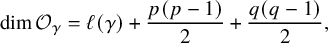 $$ \begin{align*}\dim {{\mathcal O}}_\gamma = \ell(\gamma)+\frac{p(p-1)}{2}+\frac{q(q-1)}{2}, \end{align*} $$
where
 $$ \begin{align*}\ell(\gamma): = \sum_{\substack{c_i=c_j\in {\mathbb{N}} \\ i<j}} \left(\, j-i-|\{ k\in {\mathbb{N}} \mid c_s=c_t=k \text{ for } s<i<t<j \}|\, \right) \end{align*} $$
by [Reference YamamotoYam97]. We apply this formula to compute the dimension of the irreducible Hessenberg variety $\mathrm {Hess}(\mathsf {x}_{p,q}, {\mathbf m}(w))$
. We require the following technical lemma.
$\mathrm {Hess}(\mathsf {x}_{p,q}, {\mathbf m}(w))$
. We require the following technical lemma.
Lemma 3.13. Given $w \in {\mathbf {S}}_n$
, define a sequence
$w \in {\mathbf {S}}_n$
, define a sequence ${\mathbf h}={\mathbf h}(w):=(h_1,\ldots ,h_n)$
by
${\mathbf h}={\mathbf h}(w):=(h_1,\ldots ,h_n)$
by
 $$ \begin{align*}h_i:=\max\{w(k) \mid k \leq i\}. \end{align*} $$
If w is $312$
-free, then
$312$
-free, then
 $$ \begin{align*}\ell(w)=\sum_{i=1}^n (h_i-i). \end{align*} $$
Proof. Write $w=w(1)\ldots w(n)$
in one-line notation and find k such that
$w=w(1)\ldots w(n)$
in one-line notation and find k such that $w(k)=n$
. If
$w(k)=n$
. If $n>1$
, let
$n>1$
, let $w^\prime $
be obtained from w by erasing n from the given one-line representation and let
$w^\prime $
be obtained from w by erasing n from the given one-line representation and let ${\mathbf h}^\prime $
be obtained from
${\mathbf h}^\prime $
be obtained from $w^\prime $
as
$w^\prime $
as ${\mathbf h}$
was obtained from w. For
${\mathbf h}$
was obtained from w. For $i \in [n]$
, set
$i \in [n]$
, set
 $$ \begin{align*}\mathsf{i}\mathsf{n}\mathsf{v}_i(w):=\mid \{j>i\mid w(j)<w(i)\} \mid, \end{align*} $$
and define $\mathsf {i}\mathsf {n}\mathsf {v}_i(w^\prime )$
similarly.
$\mathsf {i}\mathsf {n}\mathsf {v}_i(w^\prime )$
similarly.
We will show by induction on n that $\mathsf {i}\mathsf {n}\mathsf {v}_i(w)=h_i-i$
for every i, from which the lemma follows. The case
$\mathsf {i}\mathsf {n}\mathsf {v}_i(w)=h_i-i$
for every i, from which the lemma follows. The case $n=1$
is trivial. Assume
$n=1$
is trivial. Assume $n>1$
. We observe that if
$n>1$
. We observe that if $i \geq k$
, then
$i \geq k$
, then $w_j<w_i$
for all
$w_j<w_i$
for all $j>i$
(since w is
$j>i$
(since w is $312$
-free); hence,
$312$
-free); hence, $\mathsf {i}\mathsf {n}\mathsf {v}_i(w)=n-i=h_i-i$
. If
$\mathsf {i}\mathsf {n}\mathsf {v}_i(w)=n-i=h_i-i$
. If $i<k$
, then
$i<k$
, then
 $$ \begin{align*}\mathsf{i}\mathsf{n}\mathsf{v}_i(w)=\mathsf{i}\mathsf{n}\mathsf{v}_i(w^\prime)=h^\prime_i-i=h_i-i, \end{align*} $$
the second equality following from the inductive hypothesis.
Recall that $\pi _{{\mathbf m}(w)}$
denotes the Dyck path associated with the Hessenberg vector
$\pi _{{\mathbf m}(w)}$
denotes the Dyck path associated with the Hessenberg vector ${\mathbf m}(w)$
as in Section 2. Our work above shows that
${\mathbf m}(w)$
as in Section 2. Our work above shows that $\dim \mathrm {Hess}(\mathsf {x}_{pq}, {\mathbf m}(w))$
is given by the area of
$\dim \mathrm {Hess}(\mathsf {x}_{pq}, {\mathbf m}(w))$
is given by the area of $\pi _{{\mathbf m}(w)}$
.
$\pi _{{\mathbf m}(w)}$
.
Corollary 3.14. For each $w\in {\mathbf {S}}_q$
avoiding the pattern
$w\in {\mathbf {S}}_q$
avoiding the pattern $231$
, the Hessenberg variety
$231$
, the Hessenberg variety $\mathrm {Hess}(\mathsf {x}_{p,q}, {\mathbf m}(w))$
is irreducible of dimension
$\mathrm {Hess}(\mathsf {x}_{p,q}, {\mathbf m}(w))$
is irreducible of dimension
 $$ \begin{align} \dim \mathrm{Hess}(\mathsf{x}_{p,q},{\mathbf m}(w)) = \ell(w) + pq+ \frac{p(p-1)}{2} = \mathrm{area}(\pi_{{\mathbf m}(w)}). \end{align} $$
Proof. Recall $c_i^w=c_j^w\in {\mathbb {N}}$
if and only if
$c_i^w=c_j^w\in {\mathbb {N}}$
if and only if $j=w^{-1}(i)+p$
. Keeping also in mind that
$j=w^{-1}(i)+p$
. Keeping also in mind that $\ell (w)=\ell (w^{-1})$
, we therefore have
$\ell (w)=\ell (w^{-1})$
, we therefore have
 $$\begin{align*}|\{k\in {\mathbb{N}} \mid c_s=c_t=k \text{ for } s<i<t<w^{-1}(i)+p \}| = |\{ s<i \mid w^{-1}(s)<w^{-1}(i) \}|, \end{align*}$$
and thus,
 $$ \begin{align*} \sum_{i\in [q]} |\{k\in {\mathbb{N}} \mid c_s=c_t=k \text{ for } s<i<t<j \}| = \ell(w_0) - \ell(w^{-1})=\frac{q(q-1)}{2}-\ell(w). \end{align*} $$
We now obtain
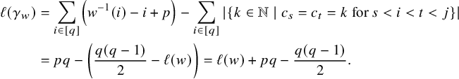 $$ \begin{align*} \ell(\gamma_w) &= \sum_{i\in [q]} \left( w^{-1}(i)-i +p \right) - \sum_{i\in [q]} |\{k\in {\mathbb{N}} \mid c_s=c_t=k \text{ for } s<i<t<j \}|\\ &= pq - \left( \frac{q(q-1)}{2}-\ell(w)\right) = \ell(w)+ pq - \frac{q(q-1)}{2}. \end{align*} $$
As $\dim \mathrm {Hess}(\mathsf {x}_{p,q},{\mathbf m}(w)) = \dim {{\mathcal O}}_{\gamma _w}$
by Theorem 3.11, this proves the first equality in (6).
$\dim \mathrm {Hess}(\mathsf {x}_{p,q},{\mathbf m}(w)) = \dim {{\mathcal O}}_{\gamma _w}$
by Theorem 3.11, this proves the first equality in (6).
To prove the second, we observe first that if ${\mathbf m}(w)=(m_1,\ldots ,m_n)$
, then
${\mathbf m}(w)=(m_1,\ldots ,m_n)$
, then
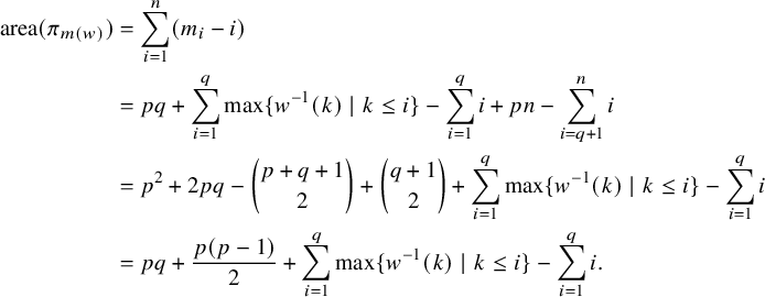 $$ \begin{align*} \mathrm{area}(\pi_{m(w)}) & = \sum_{i=1}^n (m_i-i) \\ & = pq+\sum_{i=1}^q \max\{w^{-1}(k) \mid k \leq i\}- \sum_{i=1}^q i+pn-\sum_{i=q+1}^n i \\ & = p^2+2pq-{{p+q+1} \choose {2}}+{{q+1} \choose {2}}+\sum_{i=1}^q \max\{w^{-1}(k) \mid k \leq i\}-\sum_{i=1}^q i \\ & = pq+\frac{p(p-1)}{2}+\sum_{i=1}^q \max\{w^{-1}(k) \mid k \leq i\}- \sum_{i=1}^q i. \end{align*} $$
We complete the proof by applying Lemma 3.13 to $w^{-1}$
.
$w^{-1}$
.
Remark 3.15. It follows from Corollary 3.14 and the seminal work [Reference De Mari, Procesi and ShaymanMPS92] of De Mari, Procesi and Shayman on Hessenberg varieties that if $\mathrm {Hess}(\mathsf {x}_{p,q},{\mathbf m})$
is irreducible and
$\mathrm {Hess}(\mathsf {x}_{p,q},{\mathbf m})$
is irreducible and ${\mathsf s}$
is an
${\mathsf s}$
is an $n \times n$
regular semisimple matrix, then
$n \times n$
regular semisimple matrix, then
 $$ \begin{align*}\dim\mathrm{Hess}(\mathsf{x}_{p,q},{\mathbf m})=\dim\mathrm{Hess}({\mathsf s},{\mathbf m}). \end{align*} $$
Indeed, in the case of a regular semisimple element ${\mathsf s}$
, it is easy to see from [Reference De Mari, Procesi and ShaymanMPS92, Theorem 6] that the dimension of
${\mathsf s}$
, it is easy to see from [Reference De Mari, Procesi and ShaymanMPS92, Theorem 6] that the dimension of $\mathrm {Hess}({\mathsf s},{\mathbf m})$
is precisely the area of
$\mathrm {Hess}({\mathsf s},{\mathbf m})$
is precisely the area of $\pi _{\mathbf m}$
.
$\pi _{\mathbf m}$
.
4 W-sets and cohomology classes
We turn our attention to computing the W-sets introduced in Section 2.3 above for the clans $\gamma _w$
with
$\gamma _w$
with $w\in {\mathbf {S}}_q$
. Our work below shows that the restriction of the weak order to the interval
$w\in {\mathbf {S}}_q$
. Our work below shows that the restriction of the weak order to the interval $[\gamma _e, \gamma _0]$
in
$[\gamma _e, \gamma _0]$
in $\mathbf {Clan}_{p,q}$
can be identified with the two-sided weak order on
$\mathbf {Clan}_{p,q}$
can be identified with the two-sided weak order on ${\mathbf {S}}_q$
(see Theorem 4.2 below). As a result, we give a concrete formula for the class
${\mathbf {S}}_q$
(see Theorem 4.2 below). As a result, we give a concrete formula for the class $[\overline {{{\mathcal O}}}_{\gamma _w}]$
and, in particular, the class of any Hessenberg variety
$[\overline {{{\mathcal O}}}_{\gamma _w}]$
and, in particular, the class of any Hessenberg variety $\mathrm {Hess}(\mathsf {x}_{p,q}, {\mathbf m}(w))$
. Finally, as an application of our results, we prove that the product of
$\mathrm {Hess}(\mathsf {x}_{p,q}, {\mathbf m}(w))$
. Finally, as an application of our results, we prove that the product of $[\overline {{{\mathcal O}}}_{\gamma _w}]$
with any Schubert divisor is a multiplicity-free sum of Schubert polynomials.
$[\overline {{{\mathcal O}}}_{\gamma _w}]$
with any Schubert divisor is a multiplicity-free sum of Schubert polynomials.
Recall that left weak order $\leq _L$
on the symmetric group
$\leq _L$
on the symmetric group ${\mathbf {S}}_q$
is the partial order defined by the covering relations
${\mathbf {S}}_q$
is the partial order defined by the covering relations
 $$\begin{align*}w <_L s_iw \text{ where } i\in [n-1] \text{ is such that } w^{-1}(i)<w^{-1}(i+1). \end{align*}$$
The left multiplication by $s_i$
interchanges the order of i and
$s_i$
interchanges the order of i and $i+1$
in the one-line notation for w. For example,
$i+1$
in the one-line notation for w. For example, $51324 <_L 52314$
. Similarly, the right weak order
$51324 <_L 52314$
. Similarly, the right weak order $\leq _R$
on
$\leq _R$
on ${\mathbf {S}}_q$
is the partial order defined by the covering relations
${\mathbf {S}}_q$
is the partial order defined by the covering relations
 $$\begin{align*}w <_R ws_i \text{ where } i\in [n-1] \text{ is such that } w(i)<w(i+1). \end{align*}$$
The right multiplication by $s_i$
interchanges the entries in positions i and
$s_i$
interchanges the entries in positions i and $i+1$
of the one-line notation for w. For example,
$i+1$
of the one-line notation for w. For example, $51324 <_R 53124$
.
$51324 <_R 53124$
.
We call the partial order $\preceq $
on
$\preceq $
on ${\mathbf {S}}_q$
that is generated by the covering relations of both of the left and the right weak orders the two-sided weak order on
${\mathbf {S}}_q$
that is generated by the covering relations of both of the left and the right weak orders the two-sided weak order on ${\mathbf {S}}_q$
.
${\mathbf {S}}_q$
.
Example 4.1. In Figure 3, we depict the two-sided weak order on ${\mathbf {S}}_4$
. The blue (double) edges correspond to the cover relations that are admitted by both of the orders
${\mathbf {S}}_4$
. The blue (double) edges correspond to the cover relations that are admitted by both of the orders $\leq _L$
and
$\leq _L$
and $\leq _R$
. The ordinary edges correspond to a covering relation of either
$\leq _R$
. The ordinary edges correspond to a covering relation of either $\leq _R$
or
$\leq _R$
or $\leq _L$
, but not both. Our figure shows that the two-sided weak order on
$\leq _L$
, but not both. Our figure shows that the two-sided weak order on ${\mathbf {S}}_4$
is not isomorphic to the Bruhat (i.e., inclusion) order; for example,
${\mathbf {S}}_4$
is not isomorphic to the Bruhat (i.e., inclusion) order; for example, $s_1s_2s_1 = 3214 \leq s_2s_1s_3s_2 = 3412$
in Bruhat order, but Figure 3 shows that
$s_1s_2s_1 = 3214 \leq s_2s_1s_3s_2 = 3412$
in Bruhat order, but Figure 3 shows that $3214$
is not below
$3214$
is not below $3412$
in the two-sided weak order.
$3412$
in the two-sided weak order.
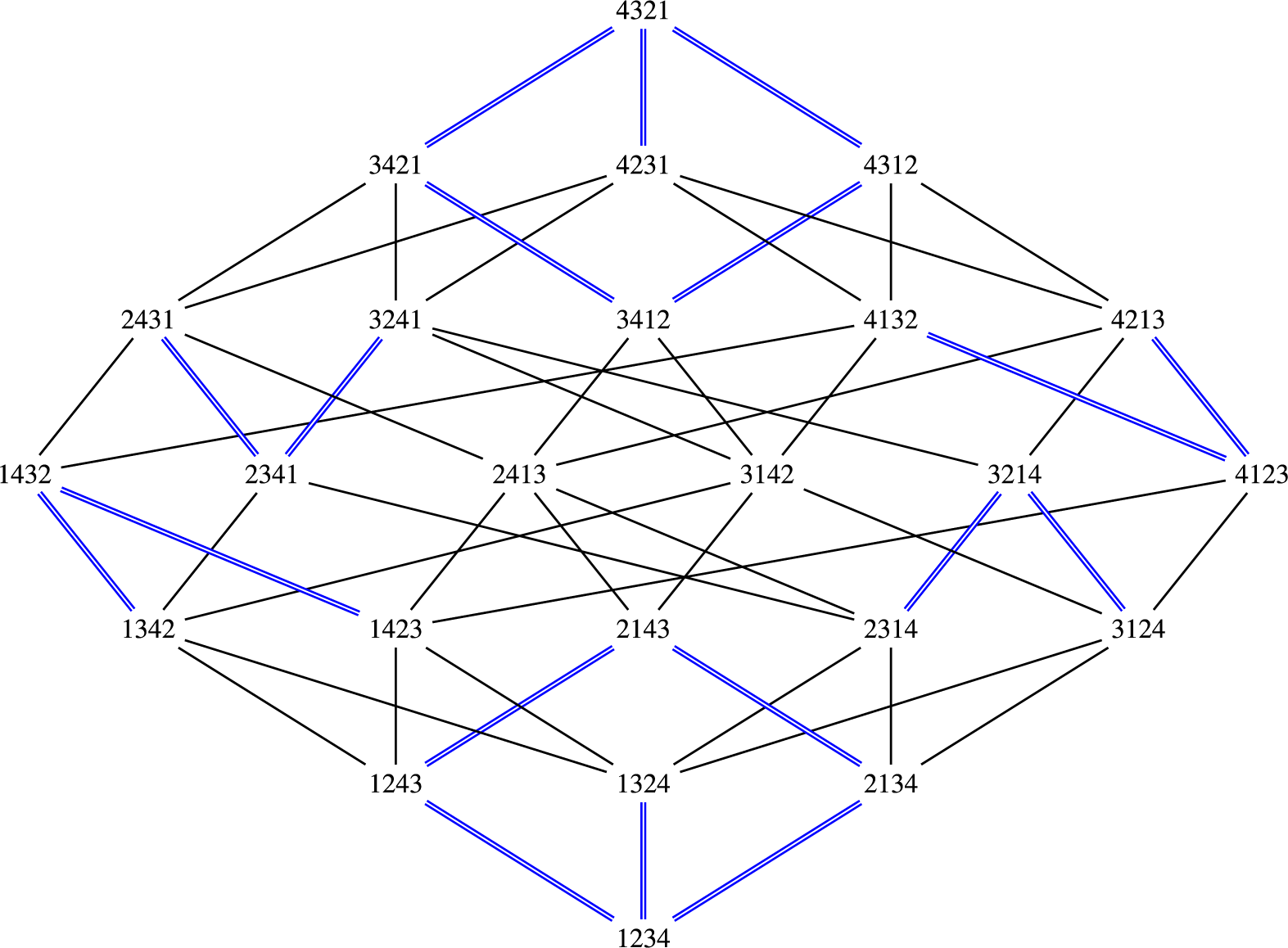
Figure 3 The two-sided weak order on ${\mathbf {S}}_4$
.
${\mathbf {S}}_4$
.
The first main result of this section is the following theorem.
Theorem 4.2. The restriction of the weak order on the interval of clans
 $$\begin{align*}[\gamma_e, \gamma_0]= \{\gamma_w \mid w\in {\mathbf{S}}_q\} \end{align*}$$
is isomorphic to the two-sided weak order on ${\mathbf {S}}_q$
.
${\mathbf {S}}_q$
.
To begin, we prove that the restriction of the weak order to the interval $[\gamma _e, \gamma _0]$
is generated by only two of the cover relations described in Section 2.3 (cf. Figure 2).
$[\gamma _e, \gamma _0]$
is generated by only two of the cover relations described in Section 2.3 (cf. Figure 2).
Lemma 4.3. Every cover relation of the weak order in the interval $[\gamma _e, \gamma _0]$
is of type IC1 or IC2.
$[\gamma _e, \gamma _0]$
is of type IC1 or IC2.
Proof. Let $\gamma _w=c_1c_2\cdots c_n \in \mathbf {Clan}_{p,q}$
for some
$\gamma _w=c_1c_2\cdots c_n \in \mathbf {Clan}_{p,q}$
for some $w\in {\mathbf {S}}_q$
. We have by definition that
$w\in {\mathbf {S}}_q$
. We have by definition that
 $$\begin{align*}c_1\cdots c_p = 12\cdots q+\cdots +, \end{align*}$$
and furthermore that no $-$
signs occur in
$-$
signs occur in $\gamma _w$
. This implies that the cover relations of types IA1, IA2 and II do not occur in the restriction of the weak order on
$\gamma _w$
. This implies that the cover relations of types IA1, IA2 and II do not occur in the restriction of the weak order on $\mathbf {Clan}_{p,q}$
to
$\mathbf {Clan}_{p,q}$
to $[\gamma _e, \gamma _0]$
. Note also that no cover relation of type IB can occur among the clans in
$[\gamma _e, \gamma _0]$
. Note also that no cover relation of type IB can occur among the clans in $[\gamma _e, \gamma _0]$
since all arcs are either nested or crossing as there is an arc connecting
$[\gamma _e, \gamma _0]$
since all arcs are either nested or crossing as there is an arc connecting $i<j$
if and only if
$i<j$
if and only if $j=w^{-1}(i)+p$
. This finishes the proof of our assertion.
$j=w^{-1}(i)+p$
. This finishes the proof of our assertion.
By the lemma, to analyze the weak order on $[\gamma _e, \gamma _0]$
, it is enough to consider cover relations of type IC1 and IC2. The following example illustrates a cover relation of each type.
$[\gamma _e, \gamma _0]$
, it is enough to consider cover relations of type IC1 and IC2. The following example illustrates a cover relation of each type.
Example 4.4. Let $p=6$
and
$p=6$
and $q=5$
. Let
$q=5$
. Let $w=51324\in {\mathbf {S}}_5$
. Figure 4 depicts the cover relation of type IC2 obtained by uncrossing the (dashed) arcs in the charged matching for
$w=51324\in {\mathbf {S}}_5$
. Figure 4 depicts the cover relation of type IC2 obtained by uncrossing the (dashed) arcs in the charged matching for $\gamma _w$
with right endpoints
$\gamma _w$
with right endpoints $8$
and
$8$
and $9$
, creating a nested pair. Note that the resulting matching corresponds to the clan
$9$
, creating a nested pair. Note that the resulting matching corresponds to the clan $\gamma _{w s_2}$
, and we have
$\gamma _{w s_2}$
, and we have $w = 51324 <_R ws_2=53124$
.
$w = 51324 <_R ws_2=53124$
.
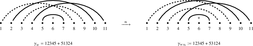
Figure 4 A cover relation of type IC2.
Similarly, we may apply a cover relation of type IC1 to $\gamma _w$
by swapping the (dashed) arcs with left endpoints
$\gamma _w$
by swapping the (dashed) arcs with left endpoints $1$
and
$1$
and $2$
, creating a nested pair. This is depicted in Figure 5. The resulting matching corresponds to clan
$2$
, creating a nested pair. This is depicted in Figure 5. The resulting matching corresponds to clan $\gamma _{s_1w}$
, and we have
$\gamma _{s_1w}$
, and we have $w=51324<_L s_1w = 52314$
.
$w=51324<_L s_1w = 52314$
.
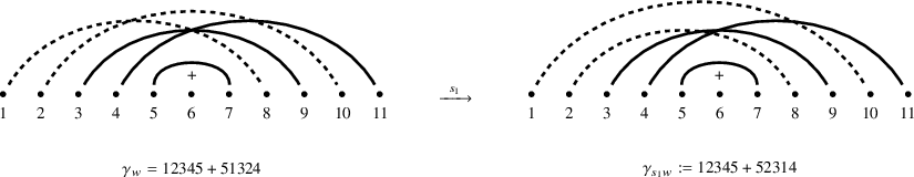
Figure 5 A cover relation of type IC1.
In the example above, we saw that each covering relation was of the form $\gamma _w \prec \gamma _{w'}$
for
$\gamma _w \prec \gamma _{w'}$
for $w,w'\in {\mathbf {S}}_5$
such that
$w,w'\in {\mathbf {S}}_5$
such that $w \prec w'$
in the two-sided weak order on
$w \prec w'$
in the two-sided weak order on ${\mathbf {S}}_5$
. This holds in greater generality and brings us to the proof of Theorem 4.2.
${\mathbf {S}}_5$
. This holds in greater generality and brings us to the proof of Theorem 4.2.
Proof of Theorem 4.2.
By Lemma 4.3, the covering relations of the weak order on $[\gamma _e,\gamma _0]$
are given by either a Type IC1 covering relation or by a Type IC2 covering relation.
$[\gamma _e,\gamma _0]$
are given by either a Type IC1 covering relation or by a Type IC2 covering relation.
Now, a covering relation of Type IC1 on clans in $[\gamma _e, \gamma _0]$
is of the form
$[\gamma _e, \gamma _0]$
is of the form
 $$ \begin{align} \gamma_w = c_1 \cdots c_{w^{-1}(i)+p} \cdots c_{w^{-1}(i+1)+p} \cdots c_n \xrightarrow{\; s_i \;} \gamma' = c_1 \cdots c_{w^{-1}(i+1)+p} \cdots c_{w^{-1}(i)+p} \cdots c_n, \end{align} $$
for some $i\in [q-1]$
such that
$i\in [q-1]$
such that $w^{-1}(i) < w^{-1}(i+1)$
. Since the resulting clan is obtained from
$w^{-1}(i) < w^{-1}(i+1)$
. Since the resulting clan is obtained from $\gamma _w$
by interchanging i and
$\gamma _w$
by interchanging i and $i+1$
in the one-line notation for w, we see that
$i+1$
in the one-line notation for w, we see that $\gamma ' = \gamma _{s_i w}$
. Similarly, a covering relation of type IC2 on clans in
$\gamma ' = \gamma _{s_i w}$
. Similarly, a covering relation of type IC2 on clans in $[\gamma _e, \gamma _0]$
is of the form
$[\gamma _e, \gamma _0]$
is of the form
 $$ \begin{align} \gamma_w = c_1 \cdots c_ic_{i+1} \cdots c_n \xrightarrow{\;s_i\;} \gamma'=c_1 \cdots c_{i+1} c_i \cdots c_n, \end{align} $$
for some $i\in \{p+1,\dots , n-1\}$
such that
$i\in \{p+1,\dots , n-1\}$
such that $w(i-p)<w(i-p+1)$
. In this case, we have
$w(i-p)<w(i-p+1)$
. In this case, we have $\gamma ' = \gamma _{ ws_{i-p}}$
since the resulting clan is obtained by interchanging the entries in the positions
$\gamma ' = \gamma _{ ws_{i-p}}$
since the resulting clan is obtained by interchanging the entries in the positions $i-p$
and
$i-p$
and $i-p+1$
in the one-line notation for w. In conclusion, we see that, for
$i-p+1$
in the one-line notation for w. In conclusion, we see that, for $w,v\in {\mathbf {S}}_q$
, if the clan
$w,v\in {\mathbf {S}}_q$
, if the clan $\gamma _w$
is covered by the clan
$\gamma _w$
is covered by the clan $\gamma _v$
in the weak order, then w is covered by v in either the right weak order or the left weak order on
$\gamma _v$
in the weak order, then w is covered by v in either the right weak order or the left weak order on ${\mathbf {S}}_q$
.
${\mathbf {S}}_q$
.
We proceed to prove the converse statement. Let $w,v\in {\mathbf {S}}_q$
be two permutations. Let
$w,v\in {\mathbf {S}}_q$
be two permutations. Let $\gamma _w=c_1^wc_2^w \cdots c_n^w$
denote the (unique) clan corresponding to w, which is defined by
$\gamma _w=c_1^wc_2^w \cdots c_n^w$
denote the (unique) clan corresponding to w, which is defined by
-
•
$c_i^w= +$
for all
$q<i \leq p$
, and -
•
$c_i^w=c_{p+w^{-1}(i)}^w=i$
for all
$i\in [q]$
.


Let $\gamma _v$
denote the unique clan corresponding to v, defined in a similar manner. Now, we assume that w is covered by v in the left weak order on
$\gamma _v$
denote the unique clan corresponding to v, defined in a similar manner. Now, we assume that w is covered by v in the left weak order on ${\mathbf {S}}_q$
. Hence,
${\mathbf {S}}_q$
. Hence, $s_iw= v$
holds for some
$s_iw= v$
holds for some $i\in [q-1]$
. After writing w and
$i\in [q-1]$
. After writing w and $s_iw$
in their one-line notations, we see that the covering relation
$s_iw$
in their one-line notations, we see that the covering relation $w\leq _L v$
corresponds to the covering relation in (7). Likewise, if w is covered by v in the right weak order in such a way that
$w\leq _L v$
corresponds to the covering relation in (7). Likewise, if w is covered by v in the right weak order in such a way that $ws_i= v$
for some
$ws_i= v$
for some $i\in [q-1]$
, then the covering relation in (8) holds. Hence, we proved that
$i\in [q-1]$
, then the covering relation in (8) holds. Hence, we proved that $\gamma _w \preceq \gamma _v$
if and only if
$\gamma _w \preceq \gamma _v$
if and only if $w\leq _L v$
or
$w\leq _L v$
or $w\leq _R v$
, as desired.
$w\leq _R v$
, as desired.
Corollary 4.5. The restriction of the weak order to $\mathbf {Clan}_{p,q}^{231}$
is isomorphic to the restriction of the two-sided weak order on
$\mathbf {Clan}_{p,q}^{231}$
is isomorphic to the restriction of the two-sided weak order on ${\mathbf {S}}_q$
to all
${\mathbf {S}}_q$
to all $231$
-free permutations.
$231$
-free permutations.
Remark 4.6. It is well known that the right weak order on the set of $231$
-free permutations is isomorphic to the Tamari lattice [Reference DrakeDra14, Theorem 1.2]. It is also well known that the Bruhat (i.e., inclusion) order on the set of
$231$
-free permutations is isomorphic to the Tamari lattice [Reference DrakeDra14, Theorem 1.2]. It is also well known that the Bruhat (i.e., inclusion) order on the set of $231$
-free permutations is isomorphic to the opposite of the Dyck path lattice [Reference Barcucci, Bernini, Ferrari and PonetiBBFP05].
$231$
-free permutations is isomorphic to the opposite of the Dyck path lattice [Reference Barcucci, Bernini, Ferrari and PonetiBBFP05].
Example 4.7. Let $p=q=3$
. Figure 6 shows the weak order on
$p=q=3$
. Figure 6 shows the weak order on $[\gamma _{123}, \gamma _{321}] \subset \mathbf {Clan}_{3,3}$
with all covering relations and corresponding clan written underneath each charged matching. The circled matching corresponds to the clan
$[\gamma _{123}, \gamma _{321}] \subset \mathbf {Clan}_{3,3}$
with all covering relations and corresponding clan written underneath each charged matching. The circled matching corresponds to the clan $\gamma _{231}$
. By removing this matching, we obtain the Hasse diagram of the two-sided weak order on
$\gamma _{231}$
. By removing this matching, we obtain the Hasse diagram of the two-sided weak order on $\mathbf {Clan}^{231}_{3,3}$
.
$\mathbf {Clan}^{231}_{3,3}$
.
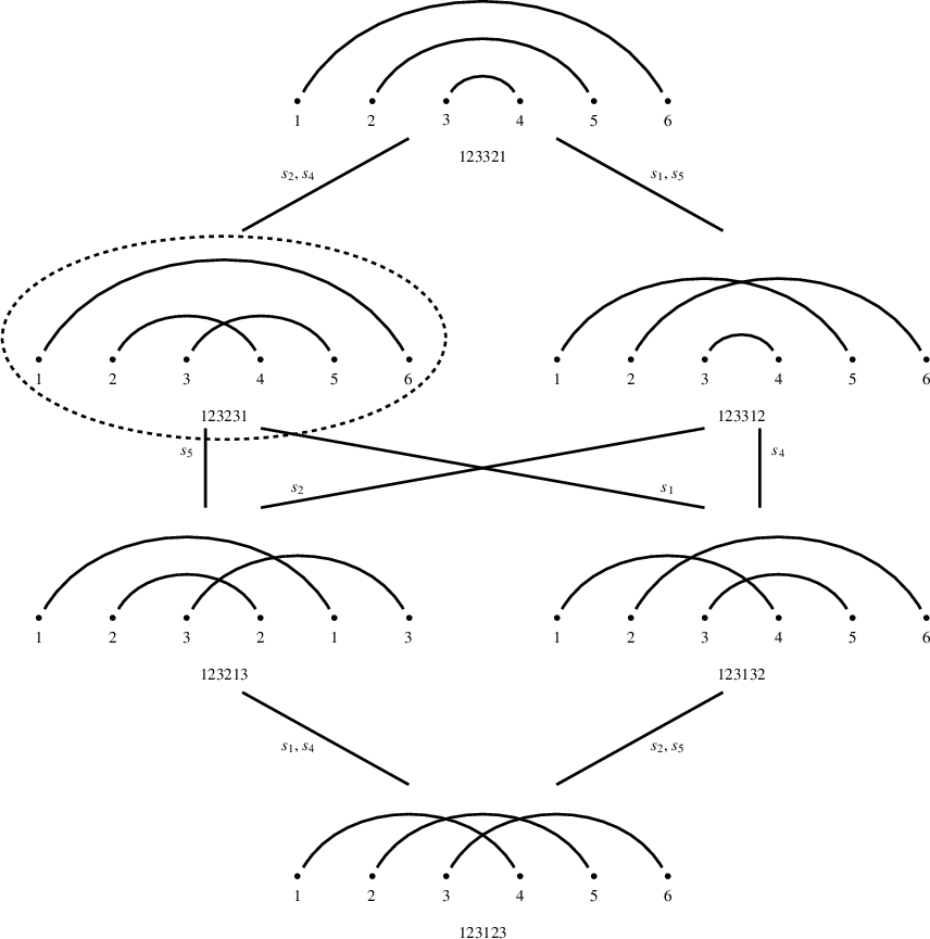
Figure 6 Weak order graph on $[\gamma _{123}, \gamma _{321}] \subset \mathbf {Clan}_{3,3}$
.
$[\gamma _{123}, \gamma _{321}] \subset \mathbf {Clan}_{3,3}$
.
With a precise description of the weak order on $[\gamma _e, \gamma _0] \subset \mathbf {Clan}_{p,q}$
in hand, we turn our attention to computing the W-sets
$[\gamma _e, \gamma _0] \subset \mathbf {Clan}_{p,q}$
in hand, we turn our attention to computing the W-sets $W(\gamma _w)$
for each
$W(\gamma _w)$
for each $w\in {\mathbf {S}}_q$
. Using Brion’s Theorem 2.11, we can use this set to obtain polynomial representatives of the cohomology classes
$w\in {\mathbf {S}}_q$
. Using Brion’s Theorem 2.11, we can use this set to obtain polynomial representatives of the cohomology classes $[\overline {{{\mathcal O}}_{\gamma _w}}]$
for each
$[\overline {{{\mathcal O}}_{\gamma _w}}]$
for each $w\in {\mathbf {S}}_q$
. If w avoids
$w\in {\mathbf {S}}_q$
. If w avoids $231$
, then we obtain, by our work in the previous section, a polynomial representative for the cohomology class of the semisimple Hessenberg variety
$231$
, then we obtain, by our work in the previous section, a polynomial representative for the cohomology class of the semisimple Hessenberg variety $\mathrm {Hess}(\mathsf {x}_{p,q}, {\mathbf m}_w)$
.
$\mathrm {Hess}(\mathsf {x}_{p,q}, {\mathbf m}_w)$
.
We begin with a lemma whose proof is evident.
Lemma 4.8. The map $\varphi : \mathbf {S}_{n}\to \mathbf {S}_{n}$
defined by
$\varphi : \mathbf {S}_{n}\to \mathbf {S}_{n}$
defined by $\varphi (v) = w_0 v^{-1} w_0$
for all
$\varphi (v) = w_0 v^{-1} w_0$
for all $v\in \mathbf {S}_{n}$
is an anti-involution. In other words, we have
$v\in \mathbf {S}_{n}$
is an anti-involution. In other words, we have $\varphi ^2 = id$
, and for all
$\varphi ^2 = id$
, and for all $v, w\in \mathbf {S}_{n}$
we have
$v, w\in \mathbf {S}_{n}$
we have $\varphi (vw) = \varphi (w)\varphi (v)$
.
$\varphi (vw) = \varphi (w)\varphi (v)$
.
Since the map $\varphi $
defined in Lemma 4.8 is an anti-involution, it is a bijection. We are interested in the restriction of
$\varphi $
defined in Lemma 4.8 is an anti-involution, it is a bijection. We are interested in the restriction of $\varphi $
to the subgroup
$\varphi $
to the subgroup $\mathbf {S}_q:= \langle s_1,\dots , s_{q-1}\rangle \hookrightarrow \mathbf {S}_{n}$
. Recall that the support
$\mathbf {S}_q:= \langle s_1,\dots , s_{q-1}\rangle \hookrightarrow \mathbf {S}_{n}$
. Recall that the support $\mathrm {Supp}(w)$
of w is the set of all simple reflections that arise in any reduced word for w.
$\mathrm {Supp}(w)$
of w is the set of all simple reflections that arise in any reduced word for w.
Lemma 4.9. The restriction of $\varphi $
to
$\varphi $
to ${\mathbf {S}}_q$
induces a bijection
${\mathbf {S}}_q$
induces a bijection $\varphi : {\mathbf {S}}_q \to \left < s_{p+1}, \ldots , s_{n-1} \right>$
. Furthermore,
$\varphi : {\mathbf {S}}_q \to \left < s_{p+1}, \ldots , s_{n-1} \right>$
. Furthermore, $\ell (v) = \ell (\varphi (v))$
for all
$\ell (v) = \ell (\varphi (v))$
for all $v\in S_q$
and
$v\in S_q$
and $\mathrm {Supp}(u)\cap \mathrm {Supp}(\varphi (v)) = \emptyset $
for all
$\mathrm {Supp}(u)\cap \mathrm {Supp}(\varphi (v)) = \emptyset $
for all $u,v\in {\mathbf {S}}_q$
.
$u,v\in {\mathbf {S}}_q$
.
Proof. Since $\varphi (s_i) = w_0 s_i w_0 = s_{n-i}$
for all
$\varphi (s_i) = w_0 s_i w_0 = s_{n-i}$
for all $i\in [n-1]$
, the first assertion of the lemma is obvious. Next, if
$i\in [n-1]$
, the first assertion of the lemma is obvious. Next, if $s_{i_1}\cdots s_{i_r}$
is a reduced expression for
$s_{i_1}\cdots s_{i_r}$
is a reduced expression for $v\in \mathbf {S}_{q}$
, then
$v\in \mathbf {S}_{q}$
, then $s_{n-i_1}\cdots s_{n-i_r}$
is a reduced expression of
$s_{n-i_1}\cdots s_{n-i_r}$
is a reduced expression of $w_0 v w_0$
. In particular,
$w_0 v w_0$
. In particular,
 $$\begin{align*}v = s_{i_1}\cdots s_{i_r} \Rightarrow \varphi(v) = s_{n-i_{r}}s_{n-i_{r-1}}\cdots s_{n-i_1}, \end{align*}$$
so $\ell (\varphi (v))=\ell (v)$
. Finally,
$\ell (\varphi (v))=\ell (v)$
. Finally, $\mathrm {Supp}(u)\subseteq \{s_1, \ldots , s_{{q-1}}\}$
and
$\mathrm {Supp}(u)\subseteq \{s_1, \ldots , s_{{q-1}}\}$
and $\mathrm {Supp}(\varphi (v)) \subseteq \{s_{p+1}, \ldots , s_{n-1}\}$
. Since
$\mathrm {Supp}(\varphi (v)) \subseteq \{s_{p+1}, \ldots , s_{n-1}\}$
. Since $q\leq p$
, we obtain the final assertion.
$q\leq p$
, we obtain the final assertion.
With these observations in place, we define a map that will allow us to compute $W(\gamma _w)$
in Theorem 4.12 below.
$W(\gamma _w)$
in Theorem 4.12 below.
Lemma 4.10. The map
 $$ \begin{align} {\mathbf{S}}_q \times {\mathbf{S}}_q \to {\mathbf{S}}_n ,\; (u,v) \mapsto u\varphi(v) \end{align} $$
is injective. Furthermore, $\ell (u\varphi (v)) = \ell (u)+ \ell (v)$
for all
$\ell (u\varphi (v)) = \ell (u)+ \ell (v)$
for all $u,v\in {\mathbf {S}}_q$
.
$u,v\in {\mathbf {S}}_q$
.
Proof. Recall from Lemma 4.9 that $\varphi $
maps
$\varphi $
maps ${\mathbf {S}}_q = \left < s_1, \ldots , s_{q-1} \right>$
to
${\mathbf {S}}_q = \left < s_1, \ldots , s_{q-1} \right>$
to $\left < s_{p+1}, \ldots , s_{n-1} \right>$
and note that the intersection of these subgroups is the trivial group since
$\left < s_{p+1}, \ldots , s_{n-1} \right>$
and note that the intersection of these subgroups is the trivial group since $q\leq p$
. Thus, if
$q\leq p$
. Thus, if $u_1,u_2,v_1,v_2\in {\mathbf {S}}_q$
such that
$u_1,u_2,v_1,v_2\in {\mathbf {S}}_q$
such that $u_1\varphi (v_1) = u_2\varphi (v_2)$
, then
$u_1\varphi (v_1) = u_2\varphi (v_2)$
, then
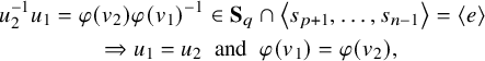 $$ \begin{align*} u_2^{-1}u_1 &= \varphi(v_2)\varphi(v_1)^{-1} \in {\mathbf{S}}_q \cap \left< s_{p+1}, \ldots, s_{n-1} \right> = \left<e\right>\\ & \quad\quad\Rightarrow u_1=u_2 \;\text{ and }\; \varphi(v_1)=\varphi(v_2), \end{align*} $$
and injectivity of the map follows. Since $\mathrm {Supp}(u)\cap \mathrm {Supp}(\varphi (v))=\emptyset $
, any reduced word for
$\mathrm {Supp}(u)\cap \mathrm {Supp}(\varphi (v))=\emptyset $
, any reduced word for $u\varphi (v)$
is the product of a reduced word of u in
$u\varphi (v)$
is the product of a reduced word of u in ${\mathbf {S}}_q$
and a reduced word for
${\mathbf {S}}_q$
and a reduced word for $\varphi (v)$
in
$\varphi (v)$
in $\left < s_{p+1}, \ldots , s_{n-1} \right>$
. Thus,
$\left < s_{p+1}, \ldots , s_{n-1} \right>$
. Thus, $\ell (u\varphi (v)) = \ell (u)+\ell (\varphi (v)) = \ell (u)+\ell (v)$
, as desired.
$\ell (u\varphi (v)) = \ell (u)+\ell (\varphi (v)) = \ell (u)+\ell (v)$
, as desired.
For each $w\in {\mathbf {S}}_q$
we define the set
$w\in {\mathbf {S}}_q$
we define the set
 $$\begin{align*}\mathcal{S}(w):= \{ (u,v)\in \mathbf{S}_q \times \mathbf{S}_q \mid\ w=uv \text{ and } \ell(w) = \ell(u)+\ell(v) \}. \end{align*}$$
Note that $\mathcal {S}(e)=\{(e,e)\}$
and
$\mathcal {S}(e)=\{(e,e)\}$
and $\mathcal {S}(s_i) = \{(e,s_i), (s_i, e)\}$
.
$\mathcal {S}(s_i) = \{(e,s_i), (s_i, e)\}$
.
Example 4.11. If $q=3$
and
$q=3$
and $w=312 = s_2s_1$
, then
$w=312 = s_2s_1$
, then $\mathcal {S}(w) = \{ (e, s_2s_1), (s_2, s_1), (s_2s_1, e) \}$
.
$\mathcal {S}(w) = \{ (e, s_2s_1), (s_2, s_1), (s_2s_1, e) \}$
.
Recall that $y_0\in {\mathbf {S}}_q$
denotes the longest element. The second main theorem of this section describes the W-sets of clans
$y_0\in {\mathbf {S}}_q$
denotes the longest element. The second main theorem of this section describes the W-sets of clans $\gamma _w$
concretely using the set
$\gamma _w$
concretely using the set $\mathcal {S}(wy_0)$
.
$\mathcal {S}(wy_0)$
.
Theorem 4.12. For all $w\in {\mathbf {S}}_q$
, the restriction of the map (9) from Lemma 4.10 to
$w\in {\mathbf {S}}_q$
, the restriction of the map (9) from Lemma 4.10 to $\mathcal {S}(wy_0)\subseteq {\mathbf {S}}_q\times {\mathbf {S}}_q$
induces a bijection
$\mathcal {S}(wy_0)\subseteq {\mathbf {S}}_q\times {\mathbf {S}}_q$
induces a bijection
 $$\begin{align*}\psi_w: \mathcal{S}(wy_0) \to W(\gamma_w) ,\; \psi_w(u,v) := u\varphi(v). \end{align*}$$
In particular, the W-set of the clan $\gamma _w$
is
$\gamma _w$
is $W(\gamma _w) = \{ u\varphi (v) \mid (u,v)\in \mathcal {S}(wy_0)\}$
.
$W(\gamma _w) = \{ u\varphi (v) \mid (u,v)\in \mathcal {S}(wy_0)\}$
.
Proof. We argue first that $\psi _w(u,v) \in W(\gamma _w)$
for all
$\psi _w(u,v) \in W(\gamma _w)$
for all $(u,v)\in \mathcal {S}(w y_0)$
. Given
$(u,v)\in \mathcal {S}(w y_0)$
. Given $(u,v)\in \mathcal {S}(w y_0)$
, let
$(u,v)\in \mathcal {S}(w y_0)$
, let $u=s_{a_1}s_{a_2}\cdots s_{a_r}$
and
$u=s_{a_1}s_{a_2}\cdots s_{a_r}$
and $v=s_{b_1}s_{b_2}\cdots s_{b_t}$
be reduced words for u and v, respectively. By assumption,
$v=s_{b_1}s_{b_2}\cdots s_{b_t}$
be reduced words for u and v, respectively. By assumption,
 $$\begin{align*}wy_0 =s_{a_1}s_{a_2}\cdots s_{a_r} s_{b_1}s_{b_2}\cdots s_{b_t} \end{align*}$$
is a reduced word for $wy_0$
. Manipulating this expression and using the fact that
$wy_0$
. Manipulating this expression and using the fact that $y_0 s_i y_0 = s_{q-i}$
for all i implies
$y_0 s_i y_0 = s_{q-i}$
for all i implies
 $$\begin{align*}s_{a_r} \cdots s_{a_2}s_{a_1} w s_{q-b_t}\cdots s_{q-b_2}s_{q-b_1} = y_0 \end{align*}$$
with $\ell (y_0) = \ell (w) + r+t$
. In particular, this expression yields a chain of length
$\ell (y_0) = \ell (w) + r+t$
. In particular, this expression yields a chain of length $r+t$
in the two-sided weak order on
$r+t$
in the two-sided weak order on ${\mathbf {S}}_q$
:
${\mathbf {S}}_q$
:
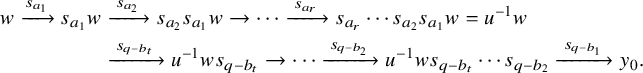 $$ \begin{align*} w \xrightarrow{ s_{a_1} } s_{a_1} w &\xrightarrow{\; s_{a_2} \; } s_{a_2}s_{a_1} w \rightarrow \cdots \xrightarrow{\; s_{a_r}\;} s_{a_r} \cdots s_{a_2}s_{a_1} w = u^{-1}w \\ & \xrightarrow{\; s_{q-b_t} \;} u^{-1}w s_{q-b_t} \rightarrow \cdots \xrightarrow{\; s_{q-b_2} \;} u^{-1}w s_{q-b_t}\cdots s_{q-b_2} \xrightarrow{\; s_{q-b_1} \;} y_0. \end{align*} $$
In this chain, left multiplication by $s_{a_k}$
is a cover in the left weak order on
$s_{a_k}$
is a cover in the left weak order on ${\mathbf {S}}_q$
and corresponds to a cover of type IC1 on clans. This cover of type IC1 on clans is labeled by the simple reflection
${\mathbf {S}}_q$
and corresponds to a cover of type IC1 on clans. This cover of type IC1 on clans is labeled by the simple reflection $s_{a_k}\in {\mathbf {S}}_n$
. Right multiplication by
$s_{a_k}\in {\mathbf {S}}_n$
. Right multiplication by $s_{b_k}$
is a cover in the right weak order on
$s_{b_k}$
is a cover in the right weak order on ${\mathbf {S}}_q$
and corresponds to a cover of type IC2 on clans. This cover of type IC2 on clans is labeled by the simple reflection
${\mathbf {S}}_q$
and corresponds to a cover of type IC2 on clans. This cover of type IC2 on clans is labeled by the simple reflection $s_{n-b_k}= \varphi (s_{b_k}) \in {\mathbf {S}}_n$
. By Theorem 4.2 and definition of the W-set, it follows that
$s_{n-b_k}= \varphi (s_{b_k}) \in {\mathbf {S}}_n$
. By Theorem 4.2 and definition of the W-set, it follows that
 $$\begin{align*}u\varphi(v) = s_{a_1} s_{a_2 } \cdots s_{a_r} s_{n-b_t} \cdots s_{n-b_2}s_{n-b_1} \in W(\gamma_w), \end{align*}$$
as desired.
To complete the proof, it suffices by Lemma 4.10 to show that $\psi _w$
is surjective. We proceed by induction on the nonnegative integer
$\psi _w$
is surjective. We proceed by induction on the nonnegative integer $\ell (wy_0)=\ell (y_0)- \ell (w)$
. If
$\ell (wy_0)=\ell (y_0)- \ell (w)$
. If $\ell (wy_0)=0$
, then
$\ell (wy_0)=0$
, then $w=y_0$
,
$w=y_0$
, $W(\gamma _w) = W(\gamma _0) = \{e\}$
, and
$W(\gamma _w) = W(\gamma _0) = \{e\}$
, and $\mathcal {S}(wy_0) = \mathcal {S}(e) = \{(e,e)\}$
. Thus, our claim holds trivially in this case.
$\mathcal {S}(wy_0) = \mathcal {S}(e) = \{(e,e)\}$
. Thus, our claim holds trivially in this case.
Suppose now that $w\in {\mathbf {S}}_q$
such that
$w\in {\mathbf {S}}_q$
such that $\ell = \ell (wy_0)>0$
and
$\ell = \ell (wy_0)>0$
and $\psi _{w'}$
is surjective for all
$\psi _{w'}$
is surjective for all $w'\in {\mathbf {S}}_q$
such that
$w'\in {\mathbf {S}}_q$
such that $\ell (w'y_0) = \ell -1$
. Since the W-set of
$\ell (w'y_0) = \ell -1$
. Since the W-set of $\gamma _w$
is obtained by multiplying the labels of the weak order cover relations along a saturated path from
$\gamma _w$
is obtained by multiplying the labels of the weak order cover relations along a saturated path from $\gamma _w$
to
$\gamma _w$
to $\gamma _0$
, if
$\gamma _0$
, if $x\in W(\gamma _w)$
, there exists
$x\in W(\gamma _w)$
, there exists $w' \in {\mathbf {S}}_q$
and
$w' \in {\mathbf {S}}_q$
and $x'\in W(\gamma _{w'})$
such that
$x'\in W(\gamma _{w'})$
such that $\gamma _w \xrightarrow {\;s_i\;} \gamma _{w'}$
and
$\gamma _w \xrightarrow {\;s_i\;} \gamma _{w'}$
and $x=s_i x'$
. By Theorem 4.2,
$x=s_i x'$
. By Theorem 4.2, $w'$
is a cover of w in the two-sided weak order on
$w'$
is a cover of w in the two-sided weak order on ${\mathbf {S}}_q$
, so
${\mathbf {S}}_q$
, so $\ell (w') = \ell (w)+1$
. This in turn implies
$\ell (w') = \ell (w)+1$
. This in turn implies $\ell (w'y_0) = \ell (wy_0)-1 = \ell -1$
, and the induction hypothesis implies that there exists
$\ell (w'y_0) = \ell (wy_0)-1 = \ell -1$
, and the induction hypothesis implies that there exists $(u,v)\in \mathcal {S}(w'y_0)$
such that
$(u,v)\in \mathcal {S}(w'y_0)$
such that $x'=u\varphi (v)$
.
$x'=u\varphi (v)$
.
There are two possible cases to consider: the cover $\gamma _w \prec \gamma _{w'}$
is either of type IC1 or IC2. If
$\gamma _w \prec \gamma _{w'}$
is either of type IC1 or IC2. If $\gamma _w \xrightarrow {\;s_i \;} \gamma _{w'}$
is a cover in the weak order on clans of type IC1, then the proof of Theorem 4.2 implies
$\gamma _w \xrightarrow {\;s_i \;} \gamma _{w'}$
is a cover in the weak order on clans of type IC1, then the proof of Theorem 4.2 implies $i\in [q-1]$
and
$i\in [q-1]$
and $w'=s_iw$
. Our assumptions also yield
$w'=s_iw$
. Our assumptions also yield
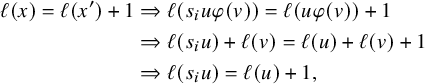 $$ \begin{align} \ell(x) = \ell(x')+1 &\Rightarrow \ell(s_iu\varphi(v) ) = \ell(u\varphi(v))+1\notag \\ &\Rightarrow \ell(s_i u) + \ell(v) = \ell(u) + \ell(v)+1\notag \\ &\Rightarrow \ell(s_i u) = \ell(u)+1, \end{align} $$
where the second implication follows from Lemma 4.10. This shows $(s_iu,v)\in \mathcal {S}(wy_0)$
since
$(s_iu,v)\in \mathcal {S}(wy_0)$
since $s_i u v= s_i w'y_0 = wy_0$
and
$s_i u v= s_i w'y_0 = wy_0$
and
 $$\begin{align*}\ell(w'y_0) = \ell(u)+\ell(v) \Rightarrow \ell (y_0) - \ell(w) -1 = \ell(u)+\ell(v) \Rightarrow \ell(wy_0) = \ell(s_iu) + \ell(v) \end{align*}$$
by (10) above. Now $x= s_i u \varphi (v) = \psi _w (s_i u,v)$
, so
$x= s_i u \varphi (v) = \psi _w (s_i u,v)$
, so $\psi _w$
is surjective in this case.
$\psi _w$
is surjective in this case.
If $\gamma _w \xrightarrow {\;s_i \;} \gamma _{w'}$
is a cover in the weak order on clans of type IC2, then the proof of Theorem 4.2 implies
$\gamma _w \xrightarrow {\;s_i \;} \gamma _{w'}$
is a cover in the weak order on clans of type IC2, then the proof of Theorem 4.2 implies $i\in \{p+1, \ldots , n-1\}$
and
$i\in \{p+1, \ldots , n-1\}$
and $w' = w s_{i-p}$
with
$w' = w s_{i-p}$
with $\ell (w')$
. Note that
$\ell (w')$
. Note that $s_i$
commutes with
$s_i$
commutes with $u\in {\mathbf {S}}_q$
and recall that
$u\in {\mathbf {S}}_q$
and recall that $s_{i} = \varphi (s_{n-i})$
. Thus,
$s_{i} = \varphi (s_{n-i})$
. Thus,
 $$ \begin{align} x = s_i x'=s_i u \varphi(v) = u s_i \varphi(v) = u \varphi(s_{n-i}) \varphi(v) = u \varphi(vs_{n-i}) \end{align} $$
by Lemma 4.8. Our assumptions also imply
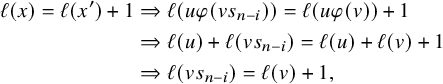 $$ \begin{align} \nonumber\ell(x) = \ell(x')+1 &\Rightarrow \ell(u \varphi(vs_{n-i})) = \ell(u\varphi(v))+1 \\ \nonumber&\Rightarrow \ell(u) + \ell(vs_{n-i}) = \ell(u) + \ell(v)+1 \\ &\Rightarrow \ell(vs_{n-i}) = \ell(v)+1, \end{align} $$
where the first implication follows from (11) and the second from Lemma 4.10. This shows $(u,vs_{n-i})\in \mathcal {S}(wy_0)$
since
$(u,vs_{n-i})\in \mathcal {S}(wy_0)$
since $uvs_{n-i} = w' y_0 s_{n-i} = w' s_{i-p} y_0 = wy_0$
and
$uvs_{n-i} = w' y_0 s_{n-i} = w' s_{i-p} y_0 = wy_0$
and
 $$\begin{align*}\ell(w'y_0)= \ell(u)+\ell(v) \Rightarrow \ell(y_0)-\ell(w)-1 = \ell(u)+\ell(v) \Rightarrow \ell(wy_0) = \ell(u) + \ell(vs_{n-i}) \end{align*}$$
by (12) above. Using (11), we conclude $x=\psi _w(u, vs_{n-1})$
so
$x=\psi _w(u, vs_{n-1})$
so $\psi _w$
is indeed surjective.
$\psi _w$
is indeed surjective.
Example 4.13. Let $q=4$
and
$q=4$
and $w=3214 = s_1s_2s_1\in {\mathbf {S}}_4$
. Then
$w=3214 = s_1s_2s_1\in {\mathbf {S}}_4$
. Then $wy_0 = 4123 = s_3s_2s_1$
and
$wy_0 = 4123 = s_3s_2s_1$
and
 $$\begin{align*}\mathcal{S}(wy_0) = \mathcal{S}(s_3s_2s_1) = \{ (s_3s_2s_1,e), (s_3s_2, s_1),(s_3, s_2s_1), (e,s_3s_2s_1) \}, \end{align*}$$
so, according to Theorem 4.12, the W-set of $\gamma _{3214}$
is
$\gamma _{3214}$
is
 $$\begin{align*}\{s_3s_2s_1, s_3s_2 s_{3+p}, s_3s_{3+p}s_{2+p}, s_{3+p}s_{2+p}s_{1+p}\}. \end{align*}$$
The interested reader can also confirm this using Theorem 4.2 and the poset pictured in Figure 3. Each element of the W-set is obtained from a saturated chain in the poset connecting $3214$
to
$3214$
to $y_0=4321$
. Covers arising from the right weak order (respectively, left weak order) on
$y_0=4321$
. Covers arising from the right weak order (respectively, left weak order) on ${\mathbf {S}}_q$
labeled by
${\mathbf {S}}_q$
labeled by $s_i$
correspond to covers in the weak order on clans labeled by
$s_i$
correspond to covers in the weak order on clans labeled by $s_{i+p}$
(respectively
$s_{i+p}$
(respectively $s_i$
). Note that there are more chains than elements of the W-set, as two chains can yield the same reduced word.
$s_i$
). Note that there are more chains than elements of the W-set, as two chains can yield the same reduced word.
We apply the results of Theorem 4.12 to compute the cohomology class of each K-orbit closure $\overline {{{\mathcal O}}}_{\gamma _w}$
. We make use of Borel’s description of the integral cohomology ring
$\overline {{{\mathcal O}}}_{\gamma _w}$
. We make use of Borel’s description of the integral cohomology ring $H^*(GL_n/B,{\mathbb {Z}})$
as the ring of coinvariants; that is,
$H^*(GL_n/B,{\mathbb {Z}})$
as the ring of coinvariants; that is,
 $$\begin{align*}H^*(GL_n/B,{\mathbb{Z}}) \simeq {\mathbb{Z}}[ x_1,\dots, x_{n}]/I, \end{align*}$$
where I is the ideal generated by the symmetric polynomials without a constant term. It is a well-known fact that the Schubert polynomial $\mathfrak {S}_w$
is a polynomial representative for the cohomology class
$\mathfrak {S}_w$
is a polynomial representative for the cohomology class $[\overline {Bw_0wB/B}]$
. For a more detailed definition of Schubert polynomials, see [Reference Lascoux and SchützenbergerLS82, Reference ManivelMan01]. Combining Theorem 4.12 with Brion’s Theorem 2.11 now yields the following.
$[\overline {Bw_0wB/B}]$
. For a more detailed definition of Schubert polynomials, see [Reference Lascoux and SchützenbergerLS82, Reference ManivelMan01]. Combining Theorem 4.12 with Brion’s Theorem 2.11 now yields the following.
Proposition 4.14. For all $w\in {\mathbf {S}}_q$
, the cohomology class of the closure of the K-orbit
$w\in {\mathbf {S}}_q$
, the cohomology class of the closure of the K-orbit ${{\mathcal O}}_{\gamma _w}$
is represented by the polynomial
${{\mathcal O}}_{\gamma _w}$
is represented by the polynomial
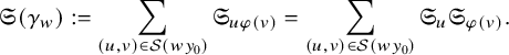 $$\begin{align*}\mathfrak{S}(\gamma_w):= \sum_{(u,v)\in \mathcal{S}(wy_0)} \mathfrak{S}_{u\varphi(v)} = \sum_{(u,v)\in \mathcal{S}(wy_0)} \mathfrak{S}_{u}\mathfrak{S}_{\varphi(v)}. \end{align*}$$
Proof. By Theorem 2.11, the polynomial representative of the cohomology class of $\overline {{{\mathcal O}}_{\gamma _w}}$
is given by the formula
$\overline {{{\mathcal O}}_{\gamma _w}}$
is given by the formula
 $$ \begin{align*} \mathfrak{S}(\gamma_w) := \sum_{x\in W(\gamma_w)} \mathfrak{S}_x, \end{align*} $$
where $\mathfrak {S}_x$
is the Schubert polynomial indexed by the permutation
$\mathfrak {S}_x$
is the Schubert polynomial indexed by the permutation $x\in {\mathbf {S}}_{n}$
. By Theorem 4.12, each
$x\in {\mathbf {S}}_{n}$
. By Theorem 4.12, each $x\in W(\gamma _w)$
can be written
$x\in W(\gamma _w)$
can be written $x = u \varphi (v)$
for a unique
$x = u \varphi (v)$
for a unique $(u,v)\in \mathcal {S}(wy_0)$
. The result now follows immediately, as u and
$(u,v)\in \mathcal {S}(wy_0)$
. The result now follows immediately, as u and $\varphi (v)$
have disjoint supports by Lemma 4.9, so
$\varphi (v)$
have disjoint supports by Lemma 4.9, so $\mathfrak {S}_{u\varphi (v)} = \mathfrak {S}_u \mathfrak {S}_{\varphi (v)}$
(see, for example, [Reference ManivelMan01, Corollary 2.4.6].)
$\mathfrak {S}_{u\varphi (v)} = \mathfrak {S}_u \mathfrak {S}_{\varphi (v)}$
(see, for example, [Reference ManivelMan01, Corollary 2.4.6].)
The following is now immediate from Theorem 3.11.
Corollary 4.15. For all $w\in {\mathbf {S}}_q$
avoiding the pattern
$w\in {\mathbf {S}}_q$
avoiding the pattern $231$
, the polynomial representative of the cohomology class of Hessenberg variety
$231$
, the polynomial representative of the cohomology class of Hessenberg variety $\mathrm {Hess}(\mathsf {x}_{p,q},{\mathbf m}(w))$
is given by
$\mathrm {Hess}(\mathsf {x}_{p,q},{\mathbf m}(w))$
is given by
 $$\begin{align*}\mathfrak{S}(\mathrm{Hess}(\mathsf{x}_{p,q}, {\mathbf m}(w)))= \sum_{(u,v)\in \mathcal{S}(wy_0)} \mathfrak{S}_{u}\mathfrak{S}_{\varphi(v)}. \end{align*}$$
Example 4.16. Let $q=3$
. For the permutation
$q=3$
. For the permutation $w=123 \in {\mathbf {S}}_3$
, the W-set of
$w=123 \in {\mathbf {S}}_3$
, the W-set of $\gamma _{123}$
is
$\gamma _{123}$
is
 $$\begin{align*}\{s_1s_2s_1, s_{p+1}s_{p+2}s_{p+1}, s_1s_2s_{p+2}, s_2s_1s_{p+1}, s_1s_{p+2}s_{p+1}, s_2s_{p+1}s_{p+2} \}.\end{align*}$$
It follows from Corollary 4.15 that the polynomial representative of the cohomology class for the Hessenberg variety $\mathrm {Hess}(\mathsf {x}_{p,3}, {\mathbf m}(123))$
is
$\mathrm {Hess}(\mathsf {x}_{p,3}, {\mathbf m}(123))$
is
 $$\begin{align*}\mathfrak{S}_{s_1s_2s_1} + \mathfrak{S}_{s_{p+1}s_{p+2}s_{p+1}} + \mathfrak{S}_{s_1s_2s_{p+2}} + \mathfrak{S}_{s_2s_1s_{p+1}} + \mathfrak{S}_{s_1s_{p+2}s_{p+1}} + \mathfrak{S}_{s_2s_{p+1}s_{p+2}}. \end{align*}$$
Applying a similar calculation to the permutation $w= 213 \in {\mathbf {S}}_3$
gives us the polynomial
$w= 213 \in {\mathbf {S}}_3$
gives us the polynomial
 $$\begin{align*}\mathfrak{S}_{s_2s_1} + \mathfrak{S}_{s_2s_{p+2}} + \mathfrak{S}_{s_{p+2}s_{p+1}}, \end{align*}$$
representing the cohomology class for the Hesseberg variety $\mathrm {Hess}(\mathsf {x}_{p,3}, {\mathbf m}(213))$
, as the W-set of
$\mathrm {Hess}(\mathsf {x}_{p,3}, {\mathbf m}(213))$
, as the W-set of $\gamma _{213}$
is
$\gamma _{213}$
is $\{s_2s_1, s_2s_{p+2}, s_{p+2}s_{p+1}\}$
.
$\{s_2s_1, s_2s_{p+2}, s_{p+2}s_{p+1}\}$
.
Our final goal is to understand the intersection of the closure of the orbit corresponding to the clan $\gamma _w$
with a ‘basic hyperplane of
$\gamma _w$
with a ‘basic hyperplane of $G L_n / B$
’. Here, by a basic hyperplane of
$G L_n / B$
’. Here, by a basic hyperplane of $G L_n / B$
, we mean the Schubert divisor
$G L_n / B$
, we mean the Schubert divisor $X_{s_iw_{0}}$
, and
$X_{s_iw_{0}}$
, and $i \in [n-1]$
. Such an intersection is succinctly expressed in the cohomology ring by Monk’s formula [Reference ManivelMan01, Theorem 2.7.1].
$i \in [n-1]$
. Such an intersection is succinctly expressed in the cohomology ring by Monk’s formula [Reference ManivelMan01, Theorem 2.7.1].
Lemma 4.17 (Monk’s formula).
For all $u \in \mathbf {S}_n$
and all
$u \in \mathbf {S}_n$
and all $m \in [n-1]$
,
$m \in [n-1]$
,
 $$ \begin{align*}\mathfrak{S}_{s_m} \mathfrak{S}_u =\sum_{\substack{j \leq m<k \\ \ell\left(u t_{j k}\right)=\ell(u)+1}} \mathfrak{S}_{u t_{j k}}, \end{align*} $$
where $t_{j k}$
is the transposition in
$t_{j k}$
is the transposition in $\mathbf {S}_n$
that interchanges j and k and leaves every other number fixed.
$\mathbf {S}_n$
that interchanges j and k and leaves every other number fixed.
Example 4.18. Let $q=3$
. We know from Example 4.16 that the cohomology class for the Hessenberg variety
$q=3$
. We know from Example 4.16 that the cohomology class for the Hessenberg variety $\mathrm {Hess}(\mathsf {x}_{p,3}, {\mathbf m}(123))$
is represented by
$\mathrm {Hess}(\mathsf {x}_{p,3}, {\mathbf m}(123))$
is represented by
 $$ \begin{align} \mathfrak{S}_{s_1s_2s_1} + \mathfrak{S}_{s_{p+1}s_{p+2}s_{p+1}} + \mathfrak{S}_{s_1s_2s_{p+2}} + \mathfrak{S}_{s_2s_1s_{p+1}} + \mathfrak{S}_{s_1s_{p+2}s_{p+1}} + \mathfrak{S}_{s_2s_{p+1}s_{p+2}}. \end{align} $$
Now, let us use Monk’s formula to understand the product $\mathfrak {S}_{s_m}\mathfrak {S}({\gamma _{123}})$
for all
$\mathfrak {S}_{s_m}\mathfrak {S}({\gamma _{123}})$
for all $m< n=6$
.
$m< n=6$
.
Monk’s formula tells us that the product of $\mathfrak {S}_{s_m}$
with each term appearing in (13) is a
$\mathfrak {S}_{s_m}$
with each term appearing in (13) is a $0-1$
sum of Schubert polynomials. Moreover, we note that the sum of these products (which constitutes the product
$0-1$
sum of Schubert polynomials. Moreover, we note that the sum of these products (which constitutes the product $\mathfrak {S}_{s_m}\mathfrak {S}({\gamma _{123}})$
) remains a
$\mathfrak {S}_{s_m}\mathfrak {S}({\gamma _{123}})$
) remains a $0-1$
sum of Schubert polynomials.
$0-1$
sum of Schubert polynomials.
Multiplying by $\mathfrak {S}_{s_1}$
gives us
$\mathfrak {S}_{s_1}$
gives us
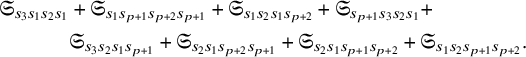 $$ \begin{align*} \mathfrak{S}_{s_3s_1s_2s_1} &+ \mathfrak{S}_{s_1s_{p+1}s_{p+2}s_{p+1}} + \mathfrak{S}_{s_1s_2s_1s_{p+2}} + \mathfrak{S}_{s_{p+1}s_3s_2s_1} +\\ &\mathfrak{S}_{s_3s_2s_1s_{p+1}} + \mathfrak{S}_{s_2s_1s_{p+2}s_{p+1}} +\mathfrak{S}_{s_2s_1s_{p+1}s_{p+2}} + \mathfrak{S}_{s_1s_2s_{p+1}s_{p+2}}. \end{align*} $$
Multiplying by $\mathfrak {S}_{s_2}$
gives us
$\mathfrak {S}_{s_2}$
gives us
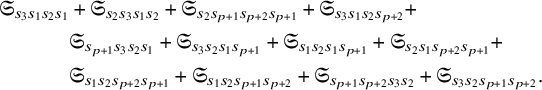 $$ \begin{align*} \mathfrak{S}_{s_3s_1s_2s_1} &+ \mathfrak{S}_{s_2s_3s_1s_2} + \mathfrak{S}_{s_2s_{p+1}s_{p+2}s_{p+1}} + \mathfrak{S}_{s_3s_1s_2s_{p+2}} + \\ &\mathfrak{S}_{s_{p+1}s_3s_2s_1} + \mathfrak{S}_{s_3s_2s_1s_{p+1}} + \mathfrak{S}_{s_1s_2s_1s_{p+1}} +\mathfrak{S}_{s_2s_1s_{p+2}s_{p+1}} +\\ &\mathfrak{S}_{s_1s_2s_{p+2}s_{p+1}} + \mathfrak{S}_{s_1s_2s_{p+1}s_{p+2}} + \mathfrak{S}_{s_{p+1}s_{p+2}s_3s_2} + \mathfrak{S}_{s_3s_2s_{p+1}s_{p+2}}. \end{align*} $$
Multiplying by $\mathfrak {S}_{s_3}$
gives us
$\mathfrak {S}_{s_3}$
gives us
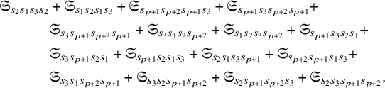 $$ \begin{align*} \mathfrak{S}_{s_2s_1s_3s_2} &+\mathfrak{S}_{s_1s_2s_1s_3} + \mathfrak{S}_{s_{p+1}s_{p+2}s_{p+1}s_3} + \mathfrak{S}_{s_{p+1}s_3s_{p+2}s_{p+1}} + \\ &\mathfrak{S}_{s_3s_{p+1}s_{p+2}s_{p+1}} + \mathfrak{S}_{s_3s_1s_2s_{p+2}} + \mathfrak{S}_{s_1s_2s_3s_{p+2}} + \mathfrak{S}_{s_{p+1}s_3s_2s_1} +\\ &\mathfrak{S}_{s_3s_{p+1}s_2s_1} + \mathfrak{S}_{s_{p+1}s_2s_1s_3} + \mathfrak{S}_{s_2s_1s_3s_{p+1}} + \mathfrak{S}_{s_{p+2}s_{p+1}s_1s_3} + \\ &\mathfrak{S}_{s_3s_1s_{p+2}s_{p+1}} + \mathfrak{S}_{s_3s_2s_{p+1}s_{p+2}} + \mathfrak{S}_{s_2s_{p+1}s_{p+2}s_3} + \mathfrak{S}_{s_2s_3s_{p+1}s_{p+2}}. \end{align*} $$
Multiplying by $\mathfrak {S}_{s_4}$
gives us
$\mathfrak {S}_{s_4}$
gives us
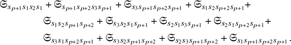 $$ \begin{align*} \mathfrak{S}_{s_{p+1}s_1s_2s_1} &+ \mathfrak{S}_{s_{p+1}s_{p+2}s_3s_{p+1}} + \mathfrak{S}_{s_3s_{p+1}s_{p+2}s_{p+1}} + \mathfrak{S}_{s_1s_2s_{p+2}s_{p+1}} + \\ &\mathfrak{S}_{s_1s_2s_{p+1}s_{p+2}} + \mathfrak{S}_{s_3s_2s_1s_{p+1}} + \mathfrak{S}_{s_2s_1s_3s_{p+1}} +\mathfrak{S}_{s_2s_1s_{p+2}s_{p+1}} +\\ &\mathfrak{S}_{s_3s_1s_{p+2}s_{p+1}} + \mathfrak{S}_{s_3s_2s_{p+1}s_{p+2}} + \mathfrak{S}_{s_2s_3s_{p+1}s_{p+2}} + \mathfrak{S}_{s_1s_{p+1}s_{p+2}s_{p+1}}. \end{align*} $$
Multiplying by $\mathfrak {S}_{s_5}$
gives us
$\mathfrak {S}_{s_5}$
gives us
 $$ \begin{align*} \mathfrak{S}_{s_3s_{p+1}s_{p+2}s_{p+1}} &+ \mathfrak{S}_{s_{p+2}s_1s_2s_1} + \mathfrak{S}_{s_1s_2s_{p+1}s_{p+2}} + \mathfrak{S}_{s_2s_1s_{p+2}s_{p+1}} +\\ &\mathfrak{S}_{s_2s_1s_{p+1}s_{p+2}} + \mathfrak{S}_{s_1s_{p+1}s_{p+2}s_{p+1}} +\mathfrak{S}_{s_3s_2s_{p+1}s_{p+2}} + \mathfrak{S}_{s_2s_3s_{p+1}s_{p+2}}. \end{align*} $$
We can use Monk’s formula to understand the product $\mathfrak {S}_{s_m}\mathfrak {S}({\gamma _w})$
in general. In particular, we show that the product
$\mathfrak {S}_{s_m}\mathfrak {S}({\gamma _w})$
in general. In particular, we show that the product $\mathfrak {S}_{s_m}\mathfrak {S}({\gamma _w})$
is always
$\mathfrak {S}_{s_m}\mathfrak {S}({\gamma _w})$
is always $0-1$
sum of Schubert polynomials for all
$0-1$
sum of Schubert polynomials for all $m < n$
.
$m < n$
.
Remark 4.19. It is shown in [Reference BrionBri05, Lemma 3.2.2] that a subvariety V of $G/B$
whose cohomology class is a 0-1 sum of Schubert classes gives a ‘multiplicity-free variety of G’ in the sense of Section 3.2 of the same reference. In turn, this property is useful for understanding the singularities (normality) of the underlying variety; see [Reference BrionBri05, Theorem 3.2.1]. Theorem 4.20 below tells us that the intersection of
$G/B$
whose cohomology class is a 0-1 sum of Schubert classes gives a ‘multiplicity-free variety of G’ in the sense of Section 3.2 of the same reference. In turn, this property is useful for understanding the singularities (normality) of the underlying variety; see [Reference BrionBri05, Theorem 3.2.1]. Theorem 4.20 below tells us that the intersection of $\mathrm {Hess}(\mathsf {x}_{p,q},{\mathbf m}(w))$
with any Schubert divisor is multiplicity free.
$\mathrm {Hess}(\mathsf {x}_{p,q},{\mathbf m}(w))$
with any Schubert divisor is multiplicity free.
Theorem 4.20. If $m \in [n-1]$
and
$m \in [n-1]$
and $w\in {\mathbf {S}}_q$
, then the product
$w\in {\mathbf {S}}_q$
, then the product $\mathfrak {S}_{s_m}\mathfrak {S}({\gamma _w})$
is a multiplicity-free sum of Schubert polynomials.
$\mathfrak {S}_{s_m}\mathfrak {S}({\gamma _w})$
is a multiplicity-free sum of Schubert polynomials.
Proof. It follows from Proposition 4.14 that
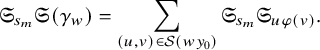 $$ \begin{align*} \mathfrak{S}_{s_m} \mathfrak{S}({\gamma_w})= \sum_{(u,v) \in \mathcal{S}(wy_0)} \mathfrak{S}_{s_m} \mathfrak{S}_{u\varphi(v)}. \end{align*} $$
We apply Monk’s formula to each product $\mathfrak {S}_{s_m}\mathfrak {S}_{u \varphi (v)}$
and obtain
$\mathfrak {S}_{s_m}\mathfrak {S}_{u \varphi (v)}$
and obtain
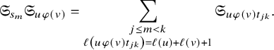 $$ \begin{align*} \mathfrak{S}_{s_m}\mathfrak{S}_{u\varphi(v)} =\displaystyle \sum_{\substack{j \leq m<k \\ \ell\left(u\varphi(v) t_{j k}\right)=\ell(u)+\ell(v)+1}} \mathfrak{S}_{u\varphi(v)t_{j k}}. \end{align*} $$
We aim to show each summand appearing on the RHS above will not appear in the corresponding sum for another pair from $\mathcal {S}(wy_0)$
.
$\mathcal {S}(wy_0)$
.
Suppose there exist pairs $(u_1,v_1)$
and
$(u_1,v_1)$
and $(u_2,v_2)$
in
$(u_2,v_2)$
in $\mathcal {S}(w)$
such that
$\mathcal {S}(w)$
such that
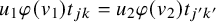 $$ \begin{align} u_1\varphi(v_1)t_{jk} = u_2\varphi(v_2)t_{j'k'} \end{align} $$
for some $j,k,j',k'$
such that
$j,k,j',k'$
such that $j\leq m<k$
and
$j\leq m<k$
and $j'\leq m<k'$
. To complete the proof, we show that (14) implies
$j'\leq m<k'$
. To complete the proof, we show that (14) implies $u_1=u_2$
and
$u_1=u_2$
and $v_1=v_2$
.
$v_1=v_2$
.
Write $x_1=u_1\varphi (v_1)$
and
$x_1=u_1\varphi (v_1)$
and $x_2=u_2\varphi (v_2)$
for the remainder of the proof. We begin with a few observations. By construction, each permutation
$x_2=u_2\varphi (v_2)$
for the remainder of the proof. We begin with a few observations. By construction, each permutation $x_i=u_i\varphi (v_i)$
with
$x_i=u_i\varphi (v_i)$
with $ i\in \{1,2\}$
satisfies
$ i\in \{1,2\}$
satisfies
 $$ \begin{align} [ q] =\{x_i(1), \ldots, x_i(q)\} \end{align} $$
and
 $$ \begin{align} x_i(a)=a \text{ for all } q+1\leq a \leq p, \end{align} $$
and
 $$ \begin{align} [n]\setminus [p] = \{x_i(p+1), \ldots, x_i(n)\}. \end{align} $$
We obtain the one-line notation of $x_1t_{jk}$
from that of
$x_1t_{jk}$
from that of $x_1$
by exchanging the entries in positions j and k and similarly for
$x_1$
by exchanging the entries in positions j and k and similarly for $x_2t_{j'k'}$
. These observations imply that pairs
$x_2t_{j'k'}$
. These observations imply that pairs $j<k$
and
$j<k$
and $j'<k'$
satisfying (14) must fall into one of the following cases:
$j'<k'$
satisfying (14) must fall into one of the following cases:
-
1.
$j,j'\in [q]$
,
$k,k'\in [n]\setminus [q]$
, -
2.
$j,j',k,k'\in [q]$
, -
3.
$j,j',k,k'\in \{q+1, \ldots , p\}$
, -
4.
$j,j'\in \{q+1, \ldots , p\}$
and
$k,k'\in [n]\setminus [p]$
, and -
5.
$j,j',k,k'\in [n]\setminus [p] $
.


Note that cases (3) and (4) do not arise when $p=q$
.
$p=q$
.
We begin with Case (1). In this case, the equality (14) and equation (15) imply
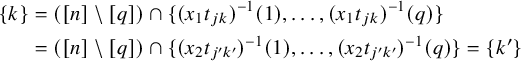 $$ \begin{align*} \{k\} &= ([n]\setminus [q]) \cap \{(x_1t_{jk})^{-1}(1), \ldots, (x_1t_{jk})^{-1}(q)\}\\ &=([n]\setminus [q]) \cap \{(x_2t_{j'k'})^{-1}(1), \ldots, (x_2t_{j'k'})^{-1}(q)\} = \{k'\} \end{align*} $$
so $k= k'$
. Similarly, using (14), (16) and (17), we have
$k= k'$
. Similarly, using (14), (16) and (17), we have
 $$ \begin{align*} \{j\} &= [q] \cap \{(x_1t_{jk})^{-1}(q+1), \ldots, (x_1t_{jk})^{-1}(n)\}\\ &=[q] \cap \{(x_2t_{j'k'})^{-1}(q+1), \ldots, (x_2t_{j'k'})^{-1}(n)\} = \{j'\} \end{align*} $$
so $j=j'$
. Now (14) implies
$j=j'$
. Now (14) implies $x_1=x_2$
, and thus,
$x_1=x_2$
, and thus, $u_1=u_2$
and
$u_1=u_2$
and $v_1=v_2$
by Lemma 4.10. Case (4) follows by similar reasoning, so we omit it to avoid repetition.
$v_1=v_2$
by Lemma 4.10. Case (4) follows by similar reasoning, so we omit it to avoid repetition.
Now suppose we are in the setting of Case (2). Then (14) becomes $u_1t_{jk}\varphi (v_1) = u_2t_{j'k'}\varphi (v_2)$
since
$u_1t_{jk}\varphi (v_1) = u_2t_{j'k'}\varphi (v_2)$
since $t_{jk}$
and
$t_{jk}$
and $t_{j'k'}$
commute with
$t_{j'k'}$
commute with $\varphi (v_1)$
and
$\varphi (v_1)$
and $\varphi (v_2)$
. By Lemma 4.9, we also know that both of the following sets
$\varphi (v_2)$
. By Lemma 4.9, we also know that both of the following sets
 $$\begin{align*}\operatorname{Supp}(u_1t_{jk}) \cap \operatorname{Supp}(\varphi(v_1))\quad\text{and}\quad \operatorname{Supp}(u_2t_{j'k'})\cap \operatorname{Supp}(\varphi(v_2)) \end{align*}$$
are empty. Consequently, $\operatorname {Supp}(\varphi (v_1)) = \operatorname {Supp}(\varphi (v_2)) $
implying that
$\operatorname {Supp}(\varphi (v_1)) = \operatorname {Supp}(\varphi (v_2)) $
implying that $\varphi (v_1)= \varphi (v_2)$
, and hence,
$\varphi (v_1)= \varphi (v_2)$
, and hence, $v_1 = v_2$
by Lemma 4.8. It now follows from the definition of the set
$v_1 = v_2$
by Lemma 4.8. It now follows from the definition of the set $\mathcal {S}(wy_0)$
that
$\mathcal {S}(wy_0)$
that $u_1=u_2$
. Indeed, we have
$u_1=u_2$
. Indeed, we have
 $$ \begin{align*}u_1v_1 = wy_0 = u_2v_2 \text{ and } v_1=v_2 \Rightarrow u_1v_1 = u_2v_1 \Rightarrow u_1=u_2.\end{align*} $$
The proof of Case (5) is almost identical to that of (2), so we omit it to avoid repetition.
Finally, we consider Case (3). The equality (14) and equation (16) immediately imply that $j=j'$
and
$j=j'$
and $k=k'$
. Thus,
$k=k'$
. Thus, $x_1=x_2$
, and we conclude
$x_1=x_2$
, and we conclude $u_1=u_2$
and
$u_1=u_2$
and $v_1=v_2$
as before. This finishes the proof of our theorem.
$v_1=v_2$
as before. This finishes the proof of our theorem.
Competing interest
The authors have no competing interests to declare.
Financial support
The first author is partially supported by a grant from the Louisiana Board of Regents (contract no. LEQSF(2021-22)-ENH-DE-26). The second author is partially supported by NSF Grant DMS-1954001 and NSF CAREER grant DMS-2237057.


 Open access