


1. Introduction
Given a graph G, a cut in G is a partition of the vertices into two parts, together with all the edges having exactly one vertex in each of the parts. The size of the cut is the number of its edges. The MaxCut problem asks for the maximum size of a cut, denoted by $\mathrm{mc}(G)$
, and it is a central problem both in discrete mathematics and theoretical computer science [Reference Alon1, Reference Alon, Krivelevich and Sudakov2, Reference Balla, Janzer and Sudakov4, Reference Edwards7, Reference Edwards8, Reference Glock, Janzer and Sudakov11, Reference Goemans and Williamson12]. If G has m edges, a simple probabilistic argument shows that the maximum cut is always at least
$\mathrm{mc}(G)$
, and it is a central problem both in discrete mathematics and theoretical computer science [Reference Alon1, Reference Alon, Krivelevich and Sudakov2, Reference Balla, Janzer and Sudakov4, Reference Edwards7, Reference Edwards8, Reference Glock, Janzer and Sudakov11, Reference Goemans and Williamson12]. If G has m edges, a simple probabilistic argument shows that the maximum cut is always at least $m/2$
, so it is natural to study the surplus, defined as
$m/2$
, so it is natural to study the surplus, defined as $\mathrm{sp}(G)=\mathrm{mc}(G)-m/2$
. A fundamental result in the area is due to Edwards [Reference Edwards7, Reference Edwards8] stating that every graph G with m edges satisfies
$\mathrm{sp}(G)=\mathrm{mc}(G)-m/2$
. A fundamental result in the area is due to Edwards [Reference Edwards7, Reference Edwards8] stating that every graph G with m edges satisfies $\mathrm{sp}(G)\geq ({\sqrt{8m+1}-1})/{8}=\Omega(m^{1/2})$
and this is tight when G is the complete graph on an odd number of vertices. The study of MaxCut in graphs avoiding a fixed graph H as a subgraph was initiated by Erdős and Lovász (see [Reference Erdős9]) in the 70’s, and substantial amount of research was devoted to this problem since then, see e.g. [Reference Alon1, Reference Alon, Krivelevich and Sudakov2, Reference Balla, Janzer and Sudakov4, Reference Glock, Janzer and Sudakov11, Reference Goemans and Williamson12].
$\mathrm{sp}(G)\geq ({\sqrt{8m+1}-1})/{8}=\Omega(m^{1/2})$
and this is tight when G is the complete graph on an odd number of vertices. The study of MaxCut in graphs avoiding a fixed graph H as a subgraph was initiated by Erdős and Lovász (see [Reference Erdős9]) in the 70’s, and substantial amount of research was devoted to this problem since then, see e.g. [Reference Alon1, Reference Alon, Krivelevich and Sudakov2, Reference Balla, Janzer and Sudakov4, Reference Glock, Janzer and Sudakov11, Reference Goemans and Williamson12].
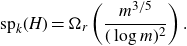
The MaxCut problem can be naturally extended to hypergraphs. If H is an r-uniform hypergraph (or r-graph, for short), a k-cut in H is a partition of the vertex set into k parts, together with all the edges having at least one vertex in each part. Similarly as before, $\mathrm{mc}_k(H)$
denotes the maximum number of edges in a k-cut. This notion was first considered by Erdös and Kleitman [Reference Erdős and Kleitman10] in 1968, and they observed that if H has m edges, then a random k-cut (i.e., where every vertex is assigned to any of the parts independently with probability
$\mathrm{mc}_k(H)$
denotes the maximum number of edges in a k-cut. This notion was first considered by Erdös and Kleitman [Reference Erdős and Kleitman10] in 1968, and they observed that if H has m edges, then a random k-cut (i.e., where every vertex is assigned to any of the parts independently with probability $1/k$
) has
$1/k$
) has $({S(r,k)k!}/{k^r})m$
edges in expectation, where S(r, k) is the Stirling number of the second kind, i.e. the number of unlabelled partitions of
$({S(r,k)k!}/{k^r})m$
edges in expectation, where S(r, k) is the Stirling number of the second kind, i.e. the number of unlabelled partitions of $\{1,\dots,r\}$
into k non-empty parts. In computer science, the problem of computing the 2-cut is known as max set splitting, or Er-set splitting if the hypergraph is r-uniform, see e.g. [Reference Guruswami14, Reference Håstad15].
$\{1,\dots,r\}$
into k non-empty parts. In computer science, the problem of computing the 2-cut is known as max set splitting, or Er-set splitting if the hypergraph is r-uniform, see e.g. [Reference Guruswami14, Reference Håstad15].
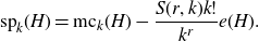
Similarly as before, we define the k-surplus of an r-graph H as
 \begin{align*}\mathrm{sp}_k(H):=\mathrm{mc}_k(H)-\frac{S(r,k)k!}{k^r}m,\end{align*}
that is, the size of the maximum k-cut of H above the expectation of the random cut. A simple extension of the methods used for graphs shows that Edwards’ lower bound holds for hypergraphs as well, that is, $\mathrm{sp}_k(H)=\Omega_r(m^{1/2})$
. However, as proved by Conlon, Fox, Kwan and Sudakov [Reference Conlon, Fox, Kwan and Sudakov6], this can be significantly improved, unless
$\mathrm{sp}_k(H)=\Omega_r(m^{1/2})$
. However, as proved by Conlon, Fox, Kwan and Sudakov [Reference Conlon, Fox, Kwan and Sudakov6], this can be significantly improved, unless $(r,k)=(3,2)$
.
$(r,k)=(3,2)$
.
Consider the case $r=3$
and
$r=3$
and $k=2$
. Let H be a 3-graph and let G be the underlying multi-graph of H, that is, we connect every pair of vertices in G by an edge as many times as it appears in an edge of H. It is easy to see that if
$k=2$
. Let H be a 3-graph and let G be the underlying multi-graph of H, that is, we connect every pair of vertices in G by an edge as many times as it appears in an edge of H. It is easy to see that if $X\cup Y$
is a partition of V(H), then H has half the number of edges in the 2-cut (X, Y) as G. Hence, the problem of 2-cuts in 3-graphs reduces to a problem about cuts in multi-graphs, and thus not much of an interest from the perspective of hypergraphs. In particular, in case H is a Steiner triple system, then G is the complete graph, thus
$X\cup Y$
is a partition of V(H), then H has half the number of edges in the 2-cut (X, Y) as G. Hence, the problem of 2-cuts in 3-graphs reduces to a problem about cuts in multi-graphs, and thus not much of an interest from the perspective of hypergraphs. In particular, in case H is a Steiner triple system, then G is the complete graph, thus $\mathrm{sp}_2(H)=\Theta(\sqrt{m})$
. Therefore, the bound of Edwards is sharp in this case. However, as it was proved by Conlon, Fox, Kwan and Sudakov [Reference Conlon, Fox, Kwan and Sudakov6], in the case of 3-cuts, we are guaranteed much larger surplus, in particular
$\mathrm{sp}_2(H)=\Theta(\sqrt{m})$
. Therefore, the bound of Edwards is sharp in this case. However, as it was proved by Conlon, Fox, Kwan and Sudakov [Reference Conlon, Fox, Kwan and Sudakov6], in the case of 3-cuts, we are guaranteed much larger surplus, in particular $\mathrm{sp}_3(H)=\Omega_r(m^{5/9})$
. We further improve this in the following theorem.
$\mathrm{sp}_3(H)=\Omega_r(m^{5/9})$
. We further improve this in the following theorem.
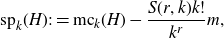
Theorem 1·1. Let H be a 3-graph with m edges. Then H has a 3-cut of size at least
 \begin{align*}\frac{2}{9}m+\Omega\left(\frac{m^{3/5}}{(\log m)^2}\right).\end{align*}
If H is the complete 3-graph on n vertices, then $m=\binom{n}{3}$
and
$m=\binom{n}{3}$
and $\mathrm{sp}_3(H)=O(n^2)$
, so
$\mathrm{sp}_3(H)=O(n^2)$
, so $\mathrm{sp}_3(H)$
might be as small as
$\mathrm{sp}_3(H)$
might be as small as $O(m^{2/3})$
. It is conjectured by Conlon, Fox, Kwan, and Sudakov [Reference Conlon, Fox, Kwan and Sudakov6] that this upper bound is sharp. A hypergraph is linear if any two of its edges intersect in at most one vertex. We prove the following stronger bound for linear 3-graphs.
$O(m^{2/3})$
. It is conjectured by Conlon, Fox, Kwan, and Sudakov [Reference Conlon, Fox, Kwan and Sudakov6] that this upper bound is sharp. A hypergraph is linear if any two of its edges intersect in at most one vertex. We prove the following stronger bound for linear 3-graphs.
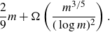
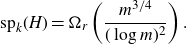
Theorem 1·2. Let H be a linear 3-graph with m edges. Then H has a 3-cut of size at least
 \begin{align*}\frac{2}{9}m+\Omega\left(\frac{m^{3/4}}{(\log m)^2}\right).\end{align*}
In case the edges of the n vertex 3-graph H are included independently with probability $n^{-1}$
, then H is close to being linear in the sense that no pair of vertices is contained in more than
$n^{-1}$
, then H is close to being linear in the sense that no pair of vertices is contained in more than $O(\log n)$
edges with positive probability. Also, it is not hard to show that
$O(\log n)$
edges with positive probability. Also, it is not hard to show that $\mathrm{sp}(H)=O(m^{3/4})$
with high probability, see Section 2·2 for a detailed argument. We believe that more sophisticated random 3-graph models can produce linear hypergraphs with similar parameters, however, we do not pursue this direction.
$\mathrm{sp}(H)=O(m^{3/4})$
with high probability, see Section 2·2 for a detailed argument. We believe that more sophisticated random 3-graph models can produce linear hypergraphs with similar parameters, however, we do not pursue this direction.
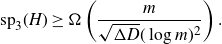
Theorems 1·1 and 1·2 can be deduced, after a bit of work, from the following general bound on the surplus of 3-graphs, which takes into account the maximum degree, and maximum co-degree.
Theorem 1·3. Let H be a 3-uniform multi-hypergraph. If H contains an induced subhypergraph with m edges, maximum degree $\Delta$
and maximum co-degree D, then
$\Delta$
and maximum co-degree D, then
 \begin{align*}\mathrm{sp}_3(H)\geq \Omega\left(\frac{m}{\sqrt{\Delta D}(\log m)^2}\right).\end{align*}
Consider the random 3-graph on n vertices, in which each edge is chosen independently with probability p, where $\log n/n^2\ll p\ll 1/n$
. With positive probability, this hypergraph satisfies
$\log n/n^2\ll p\ll 1/n$
. With positive probability, this hypergraph satisfies $\Delta=\Theta(pn^2)$
,
$\Delta=\Theta(pn^2)$
, $D=O(\log n)$
,
$D=O(\log n)$
, $m=\Theta(pn^3)$
and
$m=\Theta(pn^3)$
and $\mathrm{sp}_3(H)=O(\sqrt{p}n^2)$
, see Section 2·2 for a detailed argument. The upper bound on the surplus of this 3-graph coincides with the lower bound of Theorem 1·3 up to logarithmic factors, showing that our theorem is tight for a large family of parameters.
$\mathrm{sp}_3(H)=O(\sqrt{p}n^2)$
, see Section 2·2 for a detailed argument. The upper bound on the surplus of this 3-graph coincides with the lower bound of Theorem 1·3 up to logarithmic factors, showing that our theorem is tight for a large family of parameters.
Now let us consider k-cuts in r-graphs for $r\geq 4$
and
$r\geq 4$
and $2\leq k\leq r$
. In this case, Conlon, Fox, Kwan, and Sudakov [Reference Conlon, Fox, Kwan and Sudakov6] established the same lower bound
$2\leq k\leq r$
. In this case, Conlon, Fox, Kwan, and Sudakov [Reference Conlon, Fox, Kwan and Sudakov6] established the same lower bound $\mathrm{sp}_k(H)=\Omega_r(m^{5/9})$
. From above, they showed that if H is the random r-graph on n vertices, where each edge is included with probability
$\mathrm{sp}_k(H)=\Omega_r(m^{5/9})$
. From above, they showed that if H is the random r-graph on n vertices, where each edge is included with probability $p=\frac{1}{2}n^{-(r-3)}$
, then
$p=\frac{1}{2}n^{-(r-3)}$
, then $\mathrm{sp}_k(H)=O_r(m^{2/3})$
with high probability. This disproved the conjecture of Scott [Reference Scott18] that complete r-graphs minimize the maximum 2-cut. Moreover, it is shown in [Reference Conlon, Fox, Kwan and Sudakov6] that any general lower bound one gets for the 3-cut problem for 3-graphs extends for the k-cut problem for r-graphs if
$\mathrm{sp}_k(H)=O_r(m^{2/3})$
with high probability. This disproved the conjecture of Scott [Reference Scott18] that complete r-graphs minimize the maximum 2-cut. Moreover, it is shown in [Reference Conlon, Fox, Kwan and Sudakov6] that any general lower bound one gets for the 3-cut problem for 3-graphs extends for the k-cut problem for r-graphs if $k=r-1$
or r. In particular, we achieve the following improvements in these cases.
$k=r-1$
or r. In particular, we achieve the following improvements in these cases.
Theorem 1·4. Let $r\geq 4$
and
$r\geq 4$
and $k\in \{r-1,r\}$
. Let H be an r-graph with m edges. Then
$k\in \{r-1,r\}$
. Let H be an r-graph with m edges. Then
 \begin{align*}\mathrm{sp}_k(H)=\Omega_r\left(\frac{m^{3/5}}{(\log m)^2}\right).\end{align*}
Moreover, if H is linear, then
 \begin{align*}\mathrm{sp}_k(H)=\Omega_r\left(\frac{m^{3/4}}{(\log m)^2}\right).\end{align*}
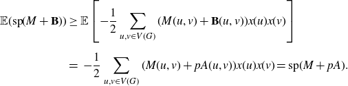
Proof overview. Let us give a brief outline of the proof of Theorem 1·3, from which all other theorems are deduced. Our approach is fairly different from that of Conlon, Fox, Kwan and Sudakov [Reference Conlon, Fox, Kwan and Sudakov6], which is based on probabilistic and combinatorial ideas. We use a combination of probabilistic and spectral techniques to bound the surplus.
First, we show that the surplus in a (multi-)graph can be lower bounded by the energy of the graph, i.e. the sum of absolute values of eigenvalues of the adjacency matrix. This quantity is extensively studied in spectral graph theory, originally introduced in theoretical chemistry. We follow the ideas of Räty, Sudakov and Tomon [Reference Räty, Sudakov and Tomon17] to relate the surplus to the energy of the graph. Then, we construct a positive semidefinite matrix based on the spectral decomposition of the adjacency matrix of the graph to show that the energy is a lower bound for the corresponding program. This can be found in Section 3. See also the recent result of Sudakov and Tomon [Reference Sudakov and Tomon19] on the Log-rank conjecture for a similar idea executed.
Now let H be a 3-uniform hypergraph for which we wish to find a large 3-cut. First, we sample a third of the vertices randomly, and write $\textbf{X}$
for the set of sampled vertices. For each
$\textbf{X}$
for the set of sampled vertices. For each $e\in E(H)$
that contains exactly one element of
$e\in E(H)$
that contains exactly one element of $\textbf{X}$
, we remove this one element, and set
$\textbf{X}$
, we remove this one element, and set $G^*$
to be the multi-graph on the vertex-set
$G^*$
to be the multi-graph on the vertex-set $V(H)\setminus \textbf{X}$
of such edges. We argue that the expected energy of
$V(H)\setminus \textbf{X}$
of such edges. We argue that the expected energy of $G^*$
is large. In order to do this, we view H as a coloured multi-graph G, in which each pair of vertices
$G^*$
is large. In order to do this, we view H as a coloured multi-graph G, in which each pair of vertices $\{u,v\}$
is included as many times as it appears in an edge
$\{u,v\}$
is included as many times as it appears in an edge $\{u,v,w\}$
of H, and whose colour is the third vertex w. Let
$\{u,v,w\}$
of H, and whose colour is the third vertex w. Let $G_1^*$
be the subgraph of G in which we keep those edges whose colour is in
$G_1^*$
be the subgraph of G in which we keep those edges whose colour is in $\textbf{X}$
. Then
$\textbf{X}$
. Then $G^*$
is an induced subgraph of
$G^*$
is an induced subgraph of $G_1^*$
, so by interlacing, it inherits certain spectral properties of
$G_1^*$
, so by interlacing, it inherits certain spectral properties of $G^*_1$
. Using matrix concentration inequalities, we show that if we randomly sample the colours in a coloured multi-graph G, the resulting graph
$G^*_1$
. Using matrix concentration inequalities, we show that if we randomly sample the colours in a coloured multi-graph G, the resulting graph $G_1^*$
is a good spectral approximation of the original graph, assuming each colour class is a low-degree graph. This, surprisingly, ensures that the energy of
$G_1^*$
is a good spectral approximation of the original graph, assuming each colour class is a low-degree graph. This, surprisingly, ensures that the energy of $G^*_1$
is large with high probability, even if G had small energy. An explanation for this and the detailed argument can be found in Section 4.
$G^*_1$
is large with high probability, even if G had small energy. An explanation for this and the detailed argument can be found in Section 4.
Now if $G^*$
has large energy, it has a large cut
$G^*$
has large energy, it has a large cut $\textbf{Y}\cup \textbf{Z}$
as well. We conclude that
$\textbf{Y}\cup \textbf{Z}$
as well. We conclude that $\textbf{X}\cup\textbf{Y}\cup \textbf{Z}$
is a partition of the vertex set of H with the required number of edges. We unite all parts of our argument and prove Theorems 1·1, 1·2, 1·3 and 1·4 in Section 5.
$\textbf{X}\cup\textbf{Y}\cup \textbf{Z}$
is a partition of the vertex set of H with the required number of edges. We unite all parts of our argument and prove Theorems 1·1, 1·2, 1·3 and 1·4 in Section 5.
2. Preliminaries
In this section, we introduce the notation used throughout our paper, which is mostly conventional, and present some basic results.
Given a vector $x\in \mathbb{R}^n$
, we write
$x\in \mathbb{R}^n$
, we write $||x||=||x||_2$
for the Euclidean norm. If
$||x||=||x||_2$
for the Euclidean norm. If $A\in \mathbb{R}^{n\times n}$
is a symmetric matrix, let
$A\in \mathbb{R}^{n\times n}$
is a symmetric matrix, let $\lambda_i(A)$
denote the i-th largest eigenvalue of A. The spectral radius of A is denoted by
$\lambda_i(A)$
denote the i-th largest eigenvalue of A. The spectral radius of A is denoted by $||A||$
, and it can be defined in a number of equivalent ways:
$||A||$
, and it can be defined in a number of equivalent ways:
 \begin{align*}||A||=\max\{|\lambda_1(A)|,|\lambda_n(A)|\}=\max_{x\in \mathbb{R}^n, ||x||=1} ||Ax||.\end{align*}
The Frobenius norm of A is defined as
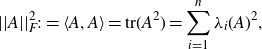 \begin{align*}||A||_F^2:=\langle A,A\rangle=\mathrm{tr}(A^2)=\sum_{i=1}^{n}\lambda_i(A)^2,\end{align*}
where $\langle A,B\rangle=\sum_{i,j}A(i,j)B(i,j)$
is the entrywise scalar product on the space of matrices.
$\langle A,B\rangle=\sum_{i,j}A(i,j)B(i,j)$
is the entrywise scalar product on the space of matrices.
2·1. Basics of cuts
In this section, we present some basic results and definitions about cuts.
It will be convenient to work with r-uniform multi-hypergraphs H (or r-multigraph for short). That is, we allow multiple edges on the same r vertices. A k-cut in H is partition of V(H) into k parts $V_1,\dots,V_k$
, together with all the edges that have at least one vertex in each of the parts. We denote by
$V_1,\dots,V_k$
, together with all the edges that have at least one vertex in each of the parts. We denote by $e(V_1,\dots,V_k)$
the number of such edges.
$e(V_1,\dots,V_k)$
the number of such edges.
Definition 2·1. The Max-k-Cut of H is the maximum size of a k-cut, and it is denoted by $\mathrm{mc}_k(H)$
.
$\mathrm{mc}_k(H)$
.
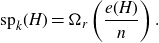
In case we consider a random partition, i.e. when each vertex of H is assigned to one of $V_i$
independently with probability
$V_i$
independently with probability $1/k$
, the expected size of a cut is
$1/k$
, the expected size of a cut is $({S(r,k)k!}/{k^r})e(H)$
, where S(r, k) is the number of unlabelled partitions of
$({S(r,k)k!}/{k^r})e(H)$
, where S(r, k) is the number of unlabelled partitions of $\{1,\dots,r\}$
into k non-empty parts.
$\{1,\dots,r\}$
into k non-empty parts.
Definition 2·2. The k-surplus of H is
 \begin{align*}\mathrm{sp}_k(H)=\mathrm{mc}_k(H)-\frac{S(r,k)k!}{k^r}e(H).\end{align*}
Clearly, $\mathrm{sp}_k(H)$
is always nonnegative. Next, we recall several basic facts from [Reference Conlon, Fox, Kwan and Sudakov6].
$\mathrm{sp}_k(H)$
is always nonnegative. Next, we recall several basic facts from [Reference Conlon, Fox, Kwan and Sudakov6].
Lemma 2·3 (Corollary 3·2 in [Reference Conlon, Fox, Kwan and Sudakov6]). Let H be an r-multigraph on n vertices. Then for every $2\leq k\leq r$
,
$2\leq k\leq r$
,
 \begin{align*}\mathrm{sp}_k(H)=\Omega_r\left(\frac{e(H)}{n}\right).\end{align*}
Lemma 2·4 (Theorem 1·4 in [Reference Conlon, Fox, Kwan and Sudakov6]). Let H be an r-multigraph on n vertices with no isolated vertices. Then for every $2\leq k\leq r$
,
$2\leq k\leq r$
,
 \begin{align*}\mathrm{sp}_{k}(H)=\Omega_r(n).\end{align*}
In the case of multi-graphs G, we write simply $\mathrm{mc}(G)$
and
$\mathrm{mc}(G)$
and $\mathrm{sp}(G)$
instead of
$\mathrm{sp}(G)$
instead of $\mathrm{mc}_2(G)$
and
$\mathrm{mc}_2(G)$
and $\mathrm{sp}_2(G)$
. We also need the following multi-graph analogue of a well-known observation, which together with its variants has been used extensively, see e.g. [Reference Alon, Krivelevich and Sudakov2, Reference Glock, Janzer and Sudakov11].
$\mathrm{sp}_2(G)$
. We also need the following multi-graph analogue of a well-known observation, which together with its variants has been used extensively, see e.g. [Reference Alon, Krivelevich and Sudakov2, Reference Glock, Janzer and Sudakov11].
Lemma 2·5. Let G be a multi-graph and let $V_1,\dots,V_k\subset V(G)$
be disjoint sets. Then
$V_1,\dots,V_k\subset V(G)$
be disjoint sets. Then
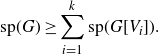 \begin{align*}\mathrm{sp}(G)\geq \sum_{i=1}^k \mathrm{sp}(G[V_i]).\end{align*}
Proof. By adding singleton sets, we may assume that the sets $V_i$
partition V(G). Let
$V_i$
partition V(G). Let $(A_i,B_i)$
be a partition of
$(A_i,B_i)$
be a partition of $V_i$
such that the number of edges between
$V_i$
such that the number of edges between $A_i$
and
$A_i$
and $B_i$
is
$B_i$
is $e(G[V_i])/2+\mathrm{sp}(G[V_i])$
. Define the random partition (X, Y) of V(G) as follows: for
$e(G[V_i])/2+\mathrm{sp}(G[V_i])$
. Define the random partition (X, Y) of V(G) as follows: for $i\in [k]$
, let either
$i\in [k]$
, let either $(X_i,Y_i)=(A_i,B_i)$
or
$(X_i,Y_i)=(A_i,B_i)$
or $(X_i,Y_i)=(B_i,A_i)$
independently with probability
$(X_i,Y_i)=(B_i,A_i)$
independently with probability $1/2$
, and let
$1/2$
, and let $X=\bigcup_{i=1}^kX_i$
and
$X=\bigcup_{i=1}^kX_i$
and $Y=\bigcup_{i=1}^k Y_i$
. It is straightforward to show that the expected number of edges in the cut given by (X, Y) is exactly
$Y=\bigcup_{i=1}^k Y_i$
. It is straightforward to show that the expected number of edges in the cut given by (X, Y) is exactly $e(G)/2+\sum_{i=1}^k\mathrm{sp}(G[V_i])$
, finishing the proof.
$e(G)/2+\sum_{i=1}^k\mathrm{sp}(G[V_i])$
, finishing the proof.
Given an r-multigraph H, for every $q\leq r$
, the underlying q-multigraph is the q-multigraph on vertex set V(H), in which each q-tuple is added as an edge as many times as it is contained in an edge of H. The final lemma in this section is used to deduce Theorem 1·4 from our results about 3-graphs.
$q\leq r$
, the underlying q-multigraph is the q-multigraph on vertex set V(H), in which each q-tuple is added as an edge as many times as it is contained in an edge of H. The final lemma in this section is used to deduce Theorem 1·4 from our results about 3-graphs.
Lemma 2·6. Let H be an r-multigraph, and let H’ be the underlying $(r-1)$
-multigraph. Then
$(r-1)$
-multigraph. Then
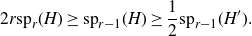 \begin{align*}2r\mathrm{sp}_{r}(H)\geq \mathrm{sp}_{r-1}(H)\geq \frac{1}{2}\mathrm{sp}_{r-1}(H').\end{align*}
Proof. We start with the first inequality. Let $U_1,\dots,U_{r-1}$
be a partition of V(H) such that
$U_1,\dots,U_{r-1}$
be a partition of V(H) such that $e_{H}(U_1,\dots,U_{r-1})=\mathrm{mc}_{r-1}(H)$
. Let
$e_{H}(U_1,\dots,U_{r-1})=\mathrm{mc}_{r-1}(H)$
. Let $V_{r}$
be a random subset of V(H), each element chosen independently with probability
$V_{r}$
be a random subset of V(H), each element chosen independently with probability $1/r$
, and let
$1/r$
, and let $V_i=U_i\setminus V_r$
for
$V_i=U_i\setminus V_r$
for $i=1,\dots,r-1$
. Note that if an edge e of H contains at least one element of each
$i=1,\dots,r-1$
. Note that if an edge e of H contains at least one element of each $U_1,\dots,U_{r-1}$
, then exactly one of these sets contains two vertices of e. Hence, the probability that e is cut by
$U_1,\dots,U_{r-1}$
, then exactly one of these sets contains two vertices of e. Hence, the probability that e is cut by $V_1,\dots,V_{r}$
is
$V_1,\dots,V_{r}$
is $c_r=2(1-\frac{1}{r})^{r-1}({1}/{r})\geq ({1}/{2r})$
. Hence,
$c_r=2(1-\frac{1}{r})^{r-1}({1}/{r})\geq ({1}/{2r})$
. Hence,
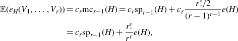 \begin{align*}\mathbb{E}(e_H(V_1,\dots,V_r))&= c_r\mathrm{mc}_{r-1}(H)=c_r\mathrm{sp}_{r-1}(H)+c_r\frac{r!/2}{(r-1)^{r-1}}e(H)\\&=c_r\mathrm{sp}_{r-1}(H)+\frac{r!}{r^r}e(H),\end{align*}
so $\mathrm{sp}_{r}(H)\geq c_r \mathrm{sp}_{r-1}(H)$
.
$\mathrm{sp}_{r}(H)\geq c_r \mathrm{sp}_{r-1}(H)$
.
Now let us prove the second inequality. Let $V_1,\dots,V_{r-1}$
be a partition of V(H) such that
$V_1,\dots,V_{r-1}$
be a partition of V(H) such that $e_{H'}(V_1,\dots,V_{r-1})=\mathrm{mc}_{r-1}(H')$
. If e is an edge of H cut by
$e_{H'}(V_1,\dots,V_{r-1})=\mathrm{mc}_{r-1}(H')$
. If e is an edge of H cut by $V_1,\dots,V_{r-1}$
, then among the
$V_1,\dots,V_{r-1}$
, then among the $(r-1)$
-element subsets of e, exactly two are cut by
$(r-1)$
-element subsets of e, exactly two are cut by $V_1,\dots,V_{r-1}$
. Thus,
$V_1,\dots,V_{r-1}$
. Thus, $e_H(V_1,\dots,V_{r-1})=({1}/{2})e_{H'}(V_1,\dots,V_{r-1})$
. Therefore,
$e_H(V_1,\dots,V_{r-1})=({1}/{2})e_{H'}(V_1,\dots,V_{r-1})$
. Therefore,
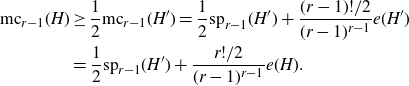 \begin{align*}\mathrm{mc}_{r-1}(H)&\geq \frac{1}{2}\mathrm{mc}_{r-1}(H')=\frac{1}{2}\mathrm{sp}_{r-1}(H')+\frac{(r-1)!/2}{(r-1)^{r-1}}e(H')\\&=\frac{1}{2}\mathrm{sp}_{r-1}(H')+\frac{r!/2}{(r-1)^{r-1}}e(H).\end{align*}
Hence, $\mathrm{sp}_{r-1}(H)\geq ({1}/{2})\mathrm{sp}_{r-1}(H').$
2·2. Probabilistic constructions
In this section, we verify our claims about the surplus of random 3-graphs.
Lemma 2·7. For every ${10\log n}/{n^2}\leq p\leq {1}/{n}$
, there exists a 3-graph H on n vertices such that H has
${10\log n}/{n^2}\leq p\leq {1}/{n}$
, there exists a 3-graph H on n vertices such that H has $\Theta(pn^3)$
edges, the maximum degree of H is
$\Theta(pn^3)$
edges, the maximum degree of H is $O(pn^2)$
, the maximum co-degree of H is
$O(pn^2)$
, the maximum co-degree of H is $O(\log n)$
, and
$O(\log n)$
, and $\mathrm{sp}_3(H)=O(\sqrt{p}n^2)$
.
$\mathrm{sp}_3(H)=O(\sqrt{p}n^2)$
.
Proof. Let p be such that ${10\log n}/{n^2}\leq p\leq {1}/{n}$
, and let H be the 3-graph on n vertices, in which each of the
${10\log n}/{n^2}\leq p\leq {1}/{n}$
, and let H be the 3-graph on n vertices, in which each of the $\binom{n}{3}$
potential edges are included independently with probability p. We assume that n is sufficiently large. By the Chernoff–Hoeffding theorem, for every
$\binom{n}{3}$
potential edges are included independently with probability p. We assume that n is sufficiently large. By the Chernoff–Hoeffding theorem, for every $x\in (0,1/2)$
, we have
$x\in (0,1/2)$
, we have
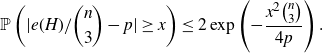 \begin{align*}\mathbb{P}\left(|e(H)/\binom{n}{3}-p|\geq x\right)\leq 2\exp\left(-\frac{x^2\binom{n}{3}}{4p}\right).\end{align*}
Hence, setting $x=20\sqrt{p}n^{-3/2}$
,
$x=20\sqrt{p}n^{-3/2}$
,
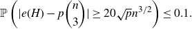 \begin{align*}\mathbb{P}\left(|e(H)-p\binom{n}{3}|\geq 20\sqrt{p}n^{3/2}\right)\leq 0.1.\end{align*}
Also, by similar concentration arguments, the maximum degree of H is at most $2p\binom{n}{2}$
with probability
$2p\binom{n}{2}$
with probability $0.9$
by our assumption
$0.9$
by our assumption $pn^2\geq 10\log n$
. Moreover, the maximum co-degree is at most
$pn^2\geq 10\log n$
. Moreover, the maximum co-degree is at most $10\log n$
with probability
$10\log n$
with probability $0.9$
by our assumption that
$0.9$
by our assumption that $p\leq 1/n$
.
$p\leq 1/n$
.
Let X, Y, Z be a partition of the vertex set into three parts, and let $N=(n/3)^3\geq |X||Y||Z|=T$
. For every
$N=(n/3)^3\geq |X||Y||Z|=T$
. For every $x\gt 0$
,
$x\gt 0$
,
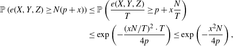 \begin{align*}\mathbb{P}\left(e(X,Y,Z)\geq N(p+x)\right)&\leq \mathbb{P}\left(\frac{e(X,Y,Z)}{T}\geq p+x\frac{N}{T}\right)\\&\leq \exp\left(-\frac{(xN/T)^2\cdot T}{4p}\right)\leq \exp\left(-\frac{x^2 N}{4p}\right),\end{align*}
where the second inequality is due to the Chernoff-Hoeffding theorem. Set $x={20\sqrt{p}}/{n}$
. The number of partitions of V(H) into three sets is at most
$x={20\sqrt{p}}/{n}$
. The number of partitions of V(H) into three sets is at most $3^n$
, so
$3^n$
, so
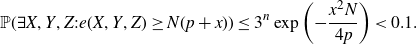 \begin{align*}\mathbb{P}(\exists X,Y,Z: e(X,Y,Z)\geq N(p+x))\leq 3^n\exp\left(-\frac{x^2 N}{4p}\right)\lt 0.1.\end{align*}
Hence, with probability 0.9, $\mathrm{mc}_3(H)\leq N(p+x)\leq pN+3\sqrt{p}n^2$
.
$\mathrm{mc}_3(H)\leq N(p+x)\leq pN+3\sqrt{p}n^2$
.
In conclusion, with positive probability, there exists a 3-graph H on n vertices such that $|e(H)-p\binom{n}{3}|\leq O(\sqrt{p}n^{3/2})$
, the maximum degree of H is at most
$|e(H)-p\binom{n}{3}|\leq O(\sqrt{p}n^{3/2})$
, the maximum degree of H is at most $pn^2$
, the maximum co-degree is at most
$pn^2$
, the maximum co-degree is at most $10\log n$
, and
$10\log n$
, and $\mathrm{mc}_3(H)\leq p({n^3}/{27})+O(\sqrt{p}n^2)$
. For such a 3-graph H, we have
$\mathrm{mc}_3(H)\leq p({n^3}/{27})+O(\sqrt{p}n^2)$
. For such a 3-graph H, we have
 \begin{align*}\mathrm{sp}_3(H)=\mathrm{mc}_3(H)-\frac{2}{9}e(H)\leq p\frac{n^3}{27}+O(\sqrt{p}n^2)-\frac{2}{9}p\binom{n}{3}+O(\sqrt{p}n^{3/2})=O(\sqrt{p}n^2).\end{align*}
In the last equality, we used that $p\cdot \frac{n^3}{27}-\frac{2}{9}p\binom{n}{3}=O(pn^2)$
.
$p\cdot \frac{n^3}{27}-\frac{2}{9}p\binom{n}{3}=O(pn^2)$
.
If one chooses $p=1/n$
, we have
$p=1/n$
, we have $m=e(H)=\Theta(n^2)$
, every co-degree in H is
$m=e(H)=\Theta(n^2)$
, every co-degree in H is $O(\log n)$
, and
$O(\log n)$
, and $\mathrm{sp}_3(H)=O(n^{3/2})=O(m^{3/4})$
, showing the almost tightness of Theorem 1·2.
$\mathrm{sp}_3(H)=O(n^{3/2})=O(m^{3/4})$
, showing the almost tightness of Theorem 1·2.
3. Surplus and Energy
In this section, we prove a lower bound on the surplus in terms of the energy of the graph. Let G be a multi-graph on vertex set V, and let $|V|=n$
. The adjacency matrix of G is the matrix
$|V|=n$
. The adjacency matrix of G is the matrix $A\in \mathbb{R}^{V\times V}$
defined as
$A\in \mathbb{R}^{V\times V}$
defined as $A(u,v)=k$
, where k is the number of edges between u and v.
$A(u,v)=k$
, where k is the number of edges between u and v.
Recall that $\mathrm{mc}(G)={e(G)}/{2}+\mathrm{sp}(G)$
. Next, we claim that
$\mathrm{mc}(G)={e(G)}/{2}+\mathrm{sp}(G)$
. Next, we claim that
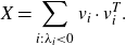
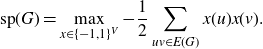 \begin{equation*} \mathrm{sp}(G)=\max_{x\in \{-1,1\}^{V}} -\frac{1}{2}\sum_{uv\in E(G)}x(u)x(v). \end{equation*}
Indeed, every $x\in \{-1,1\}^{V}$
corresponds to a partition X, Y of V(G), where
$x\in \{-1,1\}^{V}$
corresponds to a partition X, Y of V(G), where $X=\{v\in V(G):x(v)=1\}$
, and then
$X=\{v\in V(G):x(v)=1\}$
, and then
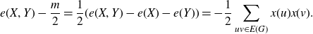 \begin{align*}e(X,Y)-\frac{m}{2}=\frac{1}{2}(e(X,Y)-e(X)-e(Y))=-\frac{1}{2}\sum_{uv\in E(G)}x(u)x(v).\end{align*}
We define the surplus of arbitrary symmetric matrices $A\in\mathbb{R}^{n\times n}$
as well. We restrict our attention to symmetric matrices, whose every diagonal entry is 0. Let
$A\in\mathbb{R}^{n\times n}$
as well. We restrict our attention to symmetric matrices, whose every diagonal entry is 0. Let
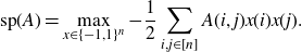 \begin{equation} \mathrm{sp}(A)=\max_{x\in \{-1,1\}^{n}} -\frac{1}{2}\sum_{i,j\in [n]}A(i,j)x(i)x(j). \end{equation}
Then $\mathrm{sp}(G)=\mathrm{sp}(A)$
if A is the adjacency matrix of G. Observe that by the condition that every diagonal entry of A is zero,
$\mathrm{sp}(G)=\mathrm{sp}(A)$
if A is the adjacency matrix of G. Observe that by the condition that every diagonal entry of A is zero, $\sum_{i,j}A(i,j)x(i)x(j)$
is a multilinear function, so its minimum on
$\sum_{i,j}A(i,j)x(i)x(j)$
is a multilinear function, so its minimum on $[{-}1,1]^n$
is attained by one of the extremal points. Therefore, (3·1) remains true if the maximum is taken over all
$[{-}1,1]^n$
is attained by one of the extremal points. Therefore, (3·1) remains true if the maximum is taken over all $x\in [{-}1,1]^{n}$
. We introduce the semidefinite relaxation of
$x\in [{-}1,1]^{n}$
. We introduce the semidefinite relaxation of $\mathrm{sp}(A)$
. Let
$\mathrm{sp}(A)$
. Let
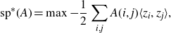 \begin{equation} \mathrm{sp}^*(A)=\max-\frac{1}{2}\sum_{i,j}A(i,j)\langle z_i,z_j\rangle,\end{equation}
where the maximum is taken over all $z_1,\dots,z_n\in\mathbb{R}^{n}$
such that
$z_1,\dots,z_n\in\mathbb{R}^{n}$
such that $||z_i||\leq 1$
for
$||z_i||\leq 1$
for $i\in [n]$
. Clearly,
$i\in [n]$
. Clearly, $\mathrm{sp}^*(A)\geq \mathrm{sp}(A).$
On the other hand, we can use the following symmetric analogue of Grothendieck’s inequality [Reference Grothendieck13] to show that
$\mathrm{sp}^*(A)\geq \mathrm{sp}(A).$
On the other hand, we can use the following symmetric analogue of Grothendieck’s inequality [Reference Grothendieck13] to show that $\mathrm{sp}^{*}(A)$
also cannot be much larger than
$\mathrm{sp}^{*}(A)$
also cannot be much larger than $\mathrm{sp}(A)$
.
$\mathrm{sp}(A)$
.
Lemma 3·1 ([Reference Alon, Makarychev, Makarychev and Naor3, Reference Charikar and Wirth5]). There exists a universal constant $C\gt 0$
such that the following holds. Let
$C\gt 0$
such that the following holds. Let $M\in \mathbb{R}^{n\times n}$
be symmetric. Let
$M\in \mathbb{R}^{n\times n}$
be symmetric. Let
 \begin{align*}\beta=\sup_{x\in [{-}1,1]^{n}}\sum M_{i,j}x(i)x(j),\end{align*}
and let
 \begin{align*}\beta^{*}=\sup_{v_1,\dots,v_n\in \mathbb{R}^{n},||v_i||\leq 1}\sum M_{i,j}\langle v_i,v_j\rangle.\end{align*}
Then $\beta\leq \beta^{*}\leq C\beta \log n$
.
$\beta\leq \beta^{*}\leq C\beta \log n$
.
Applying this lemma with the matrix $M=-({1}/{2})A$
, we get that
$M=-({1}/{2})A$
, we get that
 \begin{align*}\mathrm{sp}^*(A)\leq C\ \mathrm{sp}(A)\log n.\end{align*}
Finally, it is convenient to rewrite equation (3·2) as
 \begin{equation} \mathrm{sp}^*(A)=\max-\frac{1}{2}\langle A,X\rangle, \end{equation}
where the maximum is taken over all positive semidefinite symmetric matrices $X\in \mathbb{R}^{n\times n}$
which satisfy
$X\in \mathbb{R}^{n\times n}$
which satisfy $X(i,i)\leq 1$
for every
$X(i,i)\leq 1$
for every $i\in [n]$
. Indeed, (3·2) and (3·3) are equivalent, as if
$i\in [n]$
. Indeed, (3·2) and (3·3) are equivalent, as if $z_1,\dots,z_n\in\mathbb{R}^n$
such that
$z_1,\dots,z_n\in\mathbb{R}^n$
such that $||z_i||\leq 1$
, then the matrix X defined as
$||z_i||\leq 1$
, then the matrix X defined as $X(i,j)=\langle z_i,z_j\rangle$
is positive semidefinite and satisfies
$X(i,j)=\langle z_i,z_j\rangle$
is positive semidefinite and satisfies $X(i,i)=||z_i||^2\leq 1$
. Also, every positive semidefinite matrix X such that
$X(i,i)=||z_i||^2\leq 1$
. Also, every positive semidefinite matrix X such that $X(i,i)\leq 1$
is the Gram matrix of some vectors
$X(i,i)\leq 1$
is the Gram matrix of some vectors $z_1,\dots,z_n\in \mathbb{R}^n$
satisfying
$z_1,\dots,z_n\in \mathbb{R}^n$
satisfying $||z_i||\leq 1$
.
$||z_i||\leq 1$
.
In the next lemma, we connect the spectral properties of A to the surplus. Let $\lambda_1\geq \dots\geq \lambda_n$
be the eigenvalues of A.
$\lambda_1\geq \dots\geq \lambda_n$
be the eigenvalues of A.
Definition 3·2. The energy of $A\in \mathbb{R}^{n\times n}$
is defined as
$A\in \mathbb{R}^{n\times n}$
is defined as
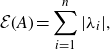 \begin{align*}\mathcal{E}(A)=\sum_{i=1}^{n}|\lambda_i|,\end{align*}
and if A is the adjacency matrix of a graph G, then the energy of G is $\mathcal{E}(G)=\mathcal{E}(A)$
.
$\mathcal{E}(G)=\mathcal{E}(A)$
.
Usually, the energy of G is denoted by E(G), but we use the notation $\mathcal{E}(G)$
to not confuse with the edge set of G, or with the expectation
$\mathcal{E}(G)$
to not confuse with the edge set of G, or with the expectation $\mathbb{E}$
. In a certain weak sense, the energy measures how random-like a graph is. Indeed, if G is a d-regular graph on n vertices, then the energy of G is at most
$\mathbb{E}$
. In a certain weak sense, the energy measures how random-like a graph is. Indeed, if G is a d-regular graph on n vertices, then the energy of G is at most $O(\sqrt{d} n)$
, and this bound is attained by the random d-regular graph. Next, we show that the energy is a lower bound (up to a constant factor) for
$O(\sqrt{d} n)$
, and this bound is attained by the random d-regular graph. Next, we show that the energy is a lower bound (up to a constant factor) for $\mathrm{sp}^*(G)$
.
$\mathrm{sp}^*(G)$
.
Lemma 3·3. If $\mathrm{tr}(A)=0$
, then
$\mathrm{tr}(A)=0$
, then $\mathrm{sp}^*(A)\geq ({1}/{4})\mathcal{E}(A).$
Proof. Let $v_1,\dots,v_n$
be an orthonormal set of eigenvectors of A such that
$v_1,\dots,v_n$
be an orthonormal set of eigenvectors of A such that $\lambda_i$
is the eigenvalue corresponding to
$\lambda_i$
is the eigenvalue corresponding to $v_i$
. Let
$v_i$
. Let
 \begin{align*}X=\sum_{i:\lambda_i\lt 0}v_i\cdot v_i^T.\end{align*}
Then X is positive semidefinite. Also, for $j=1,\dots,n$
,
$j=1,\dots,n$
,
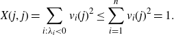 \begin{align*}X(j,j)=\sum_{i:\lambda_i\lt 0}v_i(j)^2\leq \sum_{i=1}^n v_i(j)^2=1.\end{align*}
Hence, by (3·3),
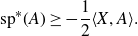 \begin{align*}\mathrm{sp}^{*}(A)\geq -\frac{1}{2}\langle X,A\rangle.\end{align*}
Observe that $A=\sum_{i=1}^{n}\lambda_i (v_i\cdot v_i^T)$
. Hence,
$A=\sum_{i=1}^{n}\lambda_i (v_i\cdot v_i^T)$
. Hence,
 \begin{align*}-\frac{1}{2}\langle X,A\rangle&=-\frac{1}{2}\left\langle \sum_{i:\lambda_i\lt 0}v_i v_i^T,\sum_{i=1}^n\lambda_iv_i v_i^T\right\rangle\\&=-\frac{1}{2}\sum_{i:\lambda_i\lt 0}\sum_{j=1}^{n}\lambda_j\langle v_i,v_j\rangle^2=-\frac{1}{2}\sum_{i:\lambda_i\lt 0}\lambda_i.\end{align*}
As $\sum_{i=1}^{n}\lambda_i=\mbox{tr}(A)=0$
, we have
$\sum_{i=1}^{n}\lambda_i=\mbox{tr}(A)=0$
, we have $\sum_{i:\lambda_i\lt 0}\lambda_i=-\frac{1}{2}\mathcal{E}(A)$
. This finishes the proof.
$\sum_{i:\lambda_i\lt 0}\lambda_i=-\frac{1}{2}\mathcal{E}(A)$
. This finishes the proof.
Corollary 3·4. If A has only zeros in the diagonal, then $\mathrm{sp}(A)=\Omega({\mathcal{E}(A)}/{\log n}).$
Finally, we note that the energy is a norm on the space of $n\times n$
symmetric matrices. On this space, the energy coincides with the Schatten 1-norm, also known as trace norm, or nuclear norm. In particular, it follows that the energy is subadditive.
$n\times n$
symmetric matrices. On this space, the energy coincides with the Schatten 1-norm, also known as trace norm, or nuclear norm. In particular, it follows that the energy is subadditive.
Lemma 3·5. Let $A,B\in \mathbb{R}^{n\times n}$
be symmetric matrices. Then
$A,B\in \mathbb{R}^{n\times n}$
be symmetric matrices. Then
 \begin{align*}\mathcal{E}(A+B)\leq \mathcal{E}(A)+\mathcal{E}(B).\end{align*}
4. Sampling coloured multi-graphs
This section is concerned with edge-coloured multi-graphs. Our goal is to show that if one randomly samples the colours in such a graph, then the resulting graph has large cuts. We use bold letters to distinguish random variables from deterministic ones. In the rest of this section, we work with the following setup.
Setup. Let G be a multi-graph with n vertices and m edges, and let $\phi:E(G)\rightarrow \mathbb{N}$
be a colouring of its edges. Let A be the adjacency matrix of G. Let
$\phi:E(G)\rightarrow \mathbb{N}$
be a colouring of its edges. Let A be the adjacency matrix of G. Let $\Delta$
be the maximum degree of G, and assume that every colour appears at most D times at every vertex for some
$\Delta$
be the maximum degree of G, and assume that every colour appears at most D times at every vertex for some $D\leq \Delta$
. Let
$D\leq \Delta$
. Let $p\in ({100}/{m},0.9)$
, and sample the colours appearing in G independently with probability p. Let
$p\in ({100}/{m},0.9)$
, and sample the colours appearing in G independently with probability p. Let $\textbf{H}$
be the sub-multi-graph of G of the sampled colours, and let
$\textbf{H}$
be the sub-multi-graph of G of the sampled colours, and let $\textbf{B}$
be the adjacency matrix of
$\textbf{B}$
be the adjacency matrix of $\textbf{H}$
.
$\textbf{H}$
.
In our first lemma, we show that pA is a good spectral approximation of $\textbf{B}$
. In order to do this, we use a result of Oliviera [Reference Oliveira16] on the concentration of matrix martingales. More precisely, we use the following direct consequence of Theorem 1·2 in [Reference Oliveira16].
$\textbf{B}$
. In order to do this, we use a result of Oliviera [Reference Oliveira16] on the concentration of matrix martingales. More precisely, we use the following direct consequence of Theorem 1·2 in [Reference Oliveira16].
Lemma 4·1 (Theorem 1·2 in [Reference Oliveira16]). Let $\textbf{M}_1,\dots,\textbf{M}_m$
be independent random
$\textbf{M}_1,\dots,\textbf{M}_m$
be independent random $n\times n$
symmetric matrices, and let
$n\times n$
symmetric matrices, and let $\textbf{P}=\textbf{M}_1+\dots+\textbf{M}_m$
. Assume that
$\textbf{P}=\textbf{M}_1+\dots+\textbf{M}_m$
. Assume that $||\textbf{M}_i||\leq D$
for
$||\textbf{M}_i||\leq D$
for $i=1,\dots,m$
, and define
$i=1,\dots,m$
, and define
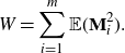 \begin{align*}W=\sum_{i=1}^m\mathbb{E}(\textbf{M}_i^2).\end{align*}
Then for all $t\gt 0$
,
$t\gt 0$
,
 \begin{align*}\mathbb{P}(||\textbf{P}-\mathbb{E}(\textbf{P})||\geq t)\leq 2n\exp\left(-\frac{t^2}{8||W||+4Dt}\right).\end{align*}
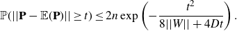
Lemma 4·2. For every $t\geq 0$
,
$t\geq 0$
,
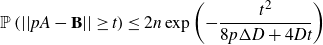
 \begin{align*}\mathbb{P}\left(||pA-\textbf{B}||\geq t\right)\leq 2n\exp\left(-\frac{t^2}{8p\Delta D+4Dt}\right).\end{align*}
Proof. Let $1,\dots,m$
be the colours of G, let
$1,\dots,m$
be the colours of G, let $A_i$
be the adjacency matrix of colour i, and let
$A_i$
be the adjacency matrix of colour i, and let $\textbf{I}_i\in \{0,1\}$
be the indicator random variable that colour i is sampled. Then setting
$\textbf{I}_i\in \{0,1\}$
be the indicator random variable that colour i is sampled. Then setting $\textbf{M}_i=\textbf{I}_i A_i$
, we have
$\textbf{M}_i=\textbf{I}_i A_i$
, we have $\textbf{B}=\textbf{M}_1+\dots+\textbf{M}_n$
. Moreover,
$\textbf{B}=\textbf{M}_1+\dots+\textbf{M}_n$
. Moreover, $||\textbf{M}_i||\leq ||A_i||\leq D$
, as the spectral radius is upper bounded by the maximum
$||\textbf{M}_i||\leq ||A_i||\leq D$
, as the spectral radius is upper bounded by the maximum $\ell_1$
-norm of the row vectors, which in turn is the maximum degree of the graph of colour i. Now let us bound
$\ell_1$
-norm of the row vectors, which in turn is the maximum degree of the graph of colour i. Now let us bound $||W||$
, where
$||W||$
, where
 \begin{align*}W=\sum_{i=1}^{m}\mathbb{E}(\textbf{M}_i^2)=p\sum_{i=1}^m A_i^2.\end{align*}
Let $\mu_1\geq \dots\geq \mu_n\geq 0$
be the eigenvalues of W. Then for every k,
$\mu_1\geq \dots\geq \mu_n\geq 0$
be the eigenvalues of W. Then for every k,
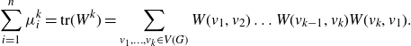 \begin{align*}\sum_{i=1}^n \mu_i^k=\mathrm{tr}(W^k)=\sum_{v_1,\dots,v_k\in V(G)}W(v_1,v_2)\dots W(v_{k-1},v_k)W(v_k,v_1).\end{align*}
Observe that $A_i^2(a,b)$
is the number of walks of length 2 between a and b using edges of colour i, so
$A_i^2(a,b)$
is the number of walks of length 2 between a and b using edges of colour i, so $W(a,b)/p=\sum_{i=1}^m A_i^2(a,b)$
is the number of monochromatic walks of length 2 between a and b in G. Hence,
$W(a,b)/p=\sum_{i=1}^m A_i^2(a,b)$
is the number of monochromatic walks of length 2 between a and b in G. Hence, $\mathrm{tr}(W^k/p^k)$
is the number of closed walks
$\mathrm{tr}(W^k/p^k)$
is the number of closed walks $(v_i,e_i,w_i,f_i)_{i=1,\dots,k}$
, where
$(v_i,e_i,w_i,f_i)_{i=1,\dots,k}$
, where $v_i,w_i$
are vertices,
$v_i,w_i$
are vertices, $e_i,f_i$
are edges,
$e_i,f_i$
are edges, $v_i,w_i$
are endpoints of
$v_i,w_i$
are endpoints of $e_i$
,
$e_i$
, $w_i,v_{i+1}$
are endpoints of
$w_i,v_{i+1}$
are endpoints of $f_i$
(where the indices are meant modulo k), and
$f_i$
(where the indices are meant modulo k), and $e_i$
and
$e_i$
and $f_i$
has the same colour. The total number of such closed walks is upper bounded by
$f_i$
has the same colour. The total number of such closed walks is upper bounded by $n\Delta^k D^k$
, as there are n choices for
$n\Delta^k D^k$
, as there are n choices for $v_1$
, if
$v_1$
, if $v_i$
is already known there are at most
$v_i$
is already known there are at most $\Delta$
choices for
$\Delta$
choices for $e_i$
and
$e_i$
and $w_i$
, and as the colour of
$w_i$
, and as the colour of $f_i$
is the same as of
$f_i$
is the same as of $e_i$
, there are at most D choices for
$e_i$
, there are at most D choices for $f_i$
and
$f_i$
and $v_{i+1}$
. Hence, we get
$v_{i+1}$
. Hence, we get
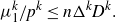 \begin{align*}\mu_1^k/p^k\leq n\Delta^k D^k.\end{align*}
As this holds for every k, we deduce that $||W||=\mu_1\leq p\Delta D$
. But then the inequality
$||W||=\mu_1\leq p\Delta D$
. But then the inequality
 \begin{align*}\mathbb{P}\left(||pA-\textbf{B}||\geq t\right)\leq 2n\exp\left(-\frac{t^2}{8p\Delta D+4Dt}\right)\end{align*}
is a straightforward consequence of Lemma 4·1.
Next, we use the previous lemma to show that the expected energy of $pA-\textbf{B}$
is large. This is somewhat counter-intuitive, as the previous lemma implies that none of the eigenvalues of
$pA-\textbf{B}$
is large. This is somewhat counter-intuitive, as the previous lemma implies that none of the eigenvalues of $pA-\textbf{B}$
is large. However, we show that the Frobenius norm of
$pA-\textbf{B}$
is large. However, we show that the Frobenius norm of $pA-\textbf{B}$
must be large in expectation, which tells us that the sum of the squares of the eigenvalues is large. Given none of the eigenvalues is large, this is only possible if the energy of
$pA-\textbf{B}$
must be large in expectation, which tells us that the sum of the squares of the eigenvalues is large. Given none of the eigenvalues is large, this is only possible if the energy of $pA-\textbf{B}$
is large as well.
$pA-\textbf{B}$
is large as well.
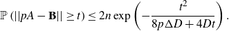
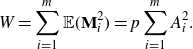
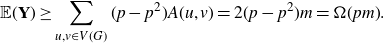
Lemma 4·3.
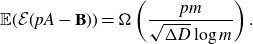 \begin{align*}\mathbb{E}(\mathcal{E}(pA-\textbf{B}))=\Omega\left(\frac{pm}{\sqrt{\Delta D}\log m}\right).\end{align*}
Proof. Let $\lambda_1\geq\dots\geq\lambda_n$
be the eigenvalues of
$\lambda_1\geq\dots\geq\lambda_n$
be the eigenvalues of $pA-\textbf{B}$
, let
$pA-\textbf{B}$
, let $\lambda=||pA-\textbf{B}||$
, and
$\lambda=||pA-\textbf{B}||$
, and $t=20\log m \sqrt{\Delta D}$
. Without loss of generality, we may assume that G has no isolated vertices, so
$t=20\log m \sqrt{\Delta D}$
. Without loss of generality, we may assume that G has no isolated vertices, so $m\geq 2n$
. But then, by the previous lemma,
$m\geq 2n$
. But then, by the previous lemma, $|\lambda_i|\leq \lambda\leq t$
with probability at least
$|\lambda_i|\leq \lambda\leq t$
with probability at least
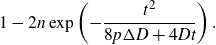 \begin{align*}1-2n\exp\left(-\frac{t^2}{8p\Delta D+4Dt}\right).\end{align*}
Here,
 \begin{align*}\frac{t^2}{8p\Delta D+4Dt}=\frac{400(\log m)^2 \Delta D}{8p\Delta D+80 D (\log m)\sqrt{\Delta D}}\geq \frac{400(\log m)^2 \Delta D}{8p\Delta D+80(\log m) \Delta D}\gt 4\log m.\end{align*}
Thus, we conclude
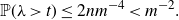 \begin{align*}\mathbb{P}(\lambda\gt t)\leq 2nm^{-4}\lt m^{-2}.\end{align*}
Consider the Frobenius norm of $pA-\textbf{B}$
. We have
$pA-\textbf{B}$
. We have
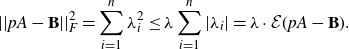 \begin{equation} ||pA-\textbf{B}||_F^2=\sum_{i=1}^{n}\lambda_i^2\leq \lambda\sum_{i=1}^{n}|\lambda_i|=\lambda\cdot \mathcal{E}(pA-\textbf{B}).\end{equation}
Let $\textbf{Y}=||pA-\textbf{B}||_F^2$
. If
$\textbf{Y}=||pA-\textbf{B}||_F^2$
. If $u,v\in V(G)$
, then
$u,v\in V(G)$
, then $\textbf{B}(u,v)=z_1\textbf{I}_1+\dots+z_r\textbf{I}_r$
, where
$\textbf{B}(u,v)=z_1\textbf{I}_1+\dots+z_r\textbf{I}_r$
, where $\textbf{I}_1,\dots,\textbf{I}_r$
are the independent indicator random variables of colours appearing between u and v in G, and
$\textbf{I}_1,\dots,\textbf{I}_r$
are the independent indicator random variables of colours appearing between u and v in G, and $z_1,\dots,z_r$
are the multiplicities of colours. Note that
$z_1,\dots,z_r$
are the multiplicities of colours. Note that $z_i\geq 1$
and
$z_i\geq 1$
and $z_1+\dots+z_r=A(u,v)$
. Hence,
$z_1+\dots+z_r=A(u,v)$
. Hence,
 \begin{align*}\mathbb{E}((pA(u,v)-\textbf{B}(u,v))^2)&=\mbox{Var}(\textbf{B}(u,v))=\sum_{i=1}^{r}\mbox{Var}(z_i\textbf{I}_r)\\&=\sum_{i=1}^{r}(p-p^2)z_i^2\geq (p-p^2)A(u,v).\end{align*}
Therefore,
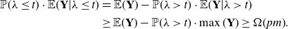
 \begin{align*}\mathbb{E}(\textbf{Y})\geq \sum_{u,v\in V(G)}(p-p^2) A(u,v)=2(p-p^2)m=\Omega(pm).\end{align*}
By (4·4), we can write
 \begin{align*}\mathbb{E}(\mathcal{E}(pA-\textbf{B}))\geq \mathbb{E}\left(\frac{\textbf{Y}}{\lambda}\right).\end{align*}
In order to bound the right-hand side, we condition on the event $(\lambda\leq t)$
:
$(\lambda\leq t)$
:
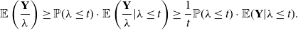 \begin{align*}\mathbb{E}\left(\frac{\textbf{Y}}{\lambda}\right)\geq \mathbb{P}(\lambda\leq t)\cdot \mathbb{E}\left(\frac{\textbf{Y}}{\lambda}| \lambda\leq t\right)\geq \frac{1}{t}\mathbb{P}(\lambda\leq t)\cdot \mathbb{E}(\textbf{Y}|\lambda\leq t).\end{align*}
Here, using that $\mathbb{P}(\lambda\gt t)\leq m^{-2}$
and
$\mathbb{P}(\lambda\gt t)\leq m^{-2}$
and $\max(\textbf{Y})\leq m^2$
, we can further write
$\max(\textbf{Y})\leq m^2$
, we can further write
 \begin{align*}\mathbb{P}(\lambda\leq t)\cdot \mathbb{E}(\textbf{Y}|\lambda\leq t)&=\mathbb{E}(\textbf{Y})-\mathbb{P}(\lambda\gt t)\cdot\mathbb{E}(\textbf{Y}|\lambda\gt t)\\&\geq \mathbb{E}(\textbf{Y})-\mathbb{P}(\lambda\gt t)\cdot\max(\textbf{Y})\geq \Omega(pm).\end{align*}
Thus, $\mathbb{E}(\mathcal{E}(pA-\textbf{B}))\geq \Omega({pm}/{t})$
, finishing the proof.
$\mathbb{E}(\mathcal{E}(pA-\textbf{B}))\geq \Omega({pm}/{t})$
, finishing the proof.
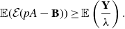
Our final technical lemma shows that $M+\textbf{B}$
has large expected surplus for any fixed matrix M.
$M+\textbf{B}$
has large expected surplus for any fixed matrix M.
Lemma 4·4. Let $M\in \mathbb{R}^{V(G)\times V(G)}$
be symmetric with only zeros in the diagonal. Then
$M\in \mathbb{R}^{V(G)\times V(G)}$
be symmetric with only zeros in the diagonal. Then
 \begin{align*}\mathbb{E}(\mathrm{sp}(M+\textbf{B}))=\Omega\left(\frac{pm}{\sqrt{\Delta D}(\log m)^2}\right).\end{align*}
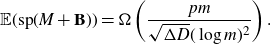
Proof. Again, we may assume that G does not contain isolated vertices. Let
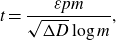 \begin{align*}t=\frac{\varepsilon pm}{\sqrt{\Delta D}\log m},\end{align*}
where $\varepsilon\gt 0$
is the constant hidden by the
$\varepsilon\gt 0$
is the constant hidden by the $\Omega(.)$
notation in Lemma 4·3. Thus,
$\Omega(.)$
notation in Lemma 4·3. Thus,
 \begin{align*}\mathbb{E}(\mathcal{E}(\textbf{B}-pA))\geq t.\end{align*}
First, assume that $\mathcal{E}(M+pA)\gt {t}/{8}$
. Then by Corollary 3·4, we have
$\mathcal{E}(M+pA)\gt {t}/{8}$
. Then by Corollary 3·4, we have $\mathrm{sp}(M+pA)=\Omega({t}/{\log n})$
. This means that there exists a vector
$\mathrm{sp}(M+pA)=\Omega({t}/{\log n})$
. This means that there exists a vector $x\in \{-1,1\}^{V(G)}$
such that
$x\in \{-1,1\}^{V(G)}$
such that
 \begin{align*}\mathrm{sp}(M+pA)=-\frac{1}{2}\sum_{u,v\in V(G)}(M(u,v)+pA(u,v))x(u)x(v)=\Omega\left(\frac{t}{\log n}\right).\end{align*}
But then
 \begin{align*} \mathbb{E}(\mathrm{sp}(M+\textbf{B}))&\geq \mathbb{E}\left[{-}\frac{1}{2}\sum_{u,v\in V(G)}(M(u,v)+\textbf{B}(u,v))x(u)x(v)\right] \\[5pt] &= \,-\frac{1}{2}\sum_{u,v\in V(G)}(M(u,v)+pA(u,v))x(u)x(v)=\mathrm{sp}(M+pA).\end{align*}
so we are done.
Hence, we may assume that $\mathcal{E}(M+pA)\leq {t}/{8}$
. Writing
$\mathcal{E}(M+pA)\leq {t}/{8}$
. Writing $(\textbf{B}-pA)=(M+\textbf{B})+(-pA-M)$
, we can use the additivity of the energy (Lemma 3·3) to deduce that
$(\textbf{B}-pA)=(M+\textbf{B})+(-pA-M)$
, we can use the additivity of the energy (Lemma 3·3) to deduce that $\mathcal{E}(\textbf{B}-pA)\leq \mathcal{E}(M+\textbf{B})+\mathcal{E}(M+pA)$
. From this,
$\mathcal{E}(\textbf{B}-pA)\leq \mathcal{E}(M+\textbf{B})+\mathcal{E}(M+pA)$
. From this,
 \begin{align*}\mathbb{E}(\mathcal{E}(M+\textbf{B}))\geq \mathbb{E}\left(\mathcal{E}(\textbf{B}-pA)-\mathcal{E}(M+pA)\right)\geq \frac{t}{2}.\end{align*}
Therefore, by Corollary 3·4,
 \begin{align*}\mathbb{E}(\mathrm{sp}(M+\textbf{B}))\geq \Omega\left(\mathbb{E}\left(\frac{\mathcal{E}(M+\textbf{B})}{\log n}\right)\right)=\Omega\left(\frac{pm}{\sqrt{\Delta D}(\log m)^2}\right).\end{align*}
In the last step, we are also using the fact that G does not contain isolated vertices, whence $m = \Omega(n)$
.
$m = \Omega(n)$
.
5. MaxCut in 3-graphs
In this section, we prove our main theorems. We start with the proof of Theorem 1·3, which we restate here for the reader’s convenience.
Theorem 5·1. Let H be a 3-multigraph. Assume that H contains an induced subghypergraph with m edges, maximum degree $\Delta$
and maximum co-degree D. Then
$\Delta$
and maximum co-degree D. Then
 \begin{align*}\mathrm{sp}_3(H)\geq \Omega\left(\frac{m}{\sqrt{\Delta D}(\log m)^2}\right).\end{align*}
Proof. Let G be the underlying multi-graph of H. For every edge $\{u,v,w\}\in E(H)$
, colour the copy of
$\{u,v,w\}\in E(H)$
, colour the copy of $\{u,v\}\in E(G)$
coming from
$\{u,v\}\in E(G)$
coming from $\{u,v,w\}$
with colour w. Let
$\{u,v,w\}$
with colour w. Let $S_0\subset V(H)$
be such that
$S_0\subset V(H)$
be such that $H[S_0]$
has m edges, maximum degree
$H[S_0]$
has m edges, maximum degree $\Delta$
, and maximum co-degree D. Let
$\Delta$
, and maximum co-degree D. Let $Q\subset S_0$
be an arbitrary set such that there are at least
$Q\subset S_0$
be an arbitrary set such that there are at least $m/3$
edges of
$m/3$
edges of $H[S_0]$
containing exactly one vertex of Q. There exists such a Q, as for a random set of vertices of
$H[S_0]$
containing exactly one vertex of Q. There exists such a Q, as for a random set of vertices of $S_0$
, sampled with probability
$S_0$
, sampled with probability $1/3$
, there are
$1/3$
, there are $4m/9$
such edges in expectation. Let
$4m/9$
such edges in expectation. Let $S=S_0\setminus Q$
.
$S=S_0\setminus Q$
.
Sample the vertices of H independently with probability $p=1/3$
, and let
$p=1/3$
, and let $\textbf{X}$
be the set of sampled vertices. First, we condition on
$\textbf{X}$
be the set of sampled vertices. First, we condition on $\textbf{X}\setminus Q$
, that is, we reveal
$\textbf{X}\setminus Q$
, that is, we reveal $\textbf{X}$
outside of Q, and treat
$\textbf{X}$
outside of Q, and treat $\textbf{X}\cap Q$
as the source of randomness. We use bold letters to denote those random variables that depend on
$\textbf{X}\cap Q$
as the source of randomness. We use bold letters to denote those random variables that depend on $\textbf{X}\cap Q$
. Let us introduce some notation, see also Figure 1 for an illustration:
$\textbf{X}\cap Q$
. Let us introduce some notation, see also Figure 1 for an illustration:
-
(1) $V=S\setminus \textbf{X}$
;
$V=S\setminus \textbf{X}$
; -
(2)
$G_0$
is the graph on vertex set V which contains those edges of G, whose colour is in Q, -
$A\in \mathbb{R}^{V\times V}$
is the adjacency matrix of
$G_0$
;
-
(3)
$\textbf{G}_0^*$
is the subgraph of
$G_0$
in which we keep those edges, whose colour is in
$ \textbf{X}\cap Q$
, -
$\textbf{B}\in \mathbb{R}^{V\times V}$
is the adjacency matrix of
$G_0^*$
;
-
(4)
$G_1^*$
is the graph on vertex set V which contains those edges of G, whose colour is in
$\textbf{X}\setminus Q$
; -
$M\in \mathbb{R}^{V\times V}$
is the adjacency matrix of
$G_1^*$
,
-
(5)
$\textbf{G}^*$
is the subgraph of
$G[\textbf{X}^c]$
, whose edges have colour in
$\textbf{X}$
. (Here,
$\textbf{X}^c=V(H)\setminus \textbf{X}$
.)


Figure 1. An illustration of the different subsets of the vertex set used in the proof of Theorem 5·1.
Note that $G_0$
has maximum degree at most
$G_0$
has maximum degree at most $2\Delta$
, as the degree of every vertex in
$2\Delta$
, as the degree of every vertex in $G_0$
is at most two times its degree in
$G_0$
is at most two times its degree in $H[S_0]$
. Also, every colour in
$H[S_0]$
. Also, every colour in $G_0$
appears at most D times at every vertex. Indeed, if some colour
$G_0$
appears at most D times at every vertex. Indeed, if some colour $q\in Q$
appears more than D times at some vertex
$q\in Q$
appears more than D times at some vertex $v\in V$
, then the co-degree of qv in
$v\in V$
, then the co-degree of qv in $H[S_0]$
is more than D, contradicting our choice of
$H[S_0]$
is more than D, contradicting our choice of $S_0$
. Thus, the matrices A and
$S_0$
. Thus, the matrices A and $\textbf{B}$
fit the Setup of Section 4.
$\textbf{B}$
fit the Setup of Section 4.
Also, $\textbf{G}^*[V]$
is the edge-disjoint union of
$\textbf{G}^*[V]$
is the edge-disjoint union of $\textbf{G}_0^*$
and
$\textbf{G}_0^*$
and $G_1^*$
, so the adjacency matrix of
$G_1^*$
, so the adjacency matrix of $\textbf{G}^*[V]$
is
$\textbf{G}^*[V]$
is $M+\textbf{B}$
. Hence,
$M+\textbf{B}$
. Hence,
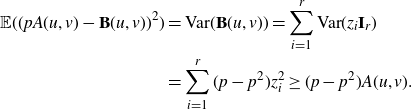
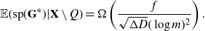
 $\mathrm{sp}(\textbf{G}^*)\geq \mathrm{sp}(\textbf{G}^*[V])=\mathrm{sp}(M+\textbf{B})$
, where the first inequality follows from Lemma 2·5. Thus, writing
$\mathrm{sp}(\textbf{G}^*)\geq \mathrm{sp}(\textbf{G}^*[V])=\mathrm{sp}(M+\textbf{B})$
, where the first inequality follows from Lemma 2·5. Thus, writing $f=e(G_0)$
, we can apply Lemma 4·4 to get
$f=e(G_0)$
, we can apply Lemma 4·4 to get
 \begin{align*}\mathbb{E}(\mathrm{sp}(\textbf{G}^*)|\textbf{X}\setminus Q)\geq \mathbb{E}(\mathrm{sp}(M+\textbf{B})|\textbf{X}\setminus Q)=\Omega\left(\frac{f}{\sqrt{\Delta D}(\log f)^2}\right). \end{align*}
As we have $f\leq m$
,
$f\leq m$
,
 \begin{align*}\mathbb{E}(\mathrm{sp}(\textbf{G}^*)|\textbf{X}\setminus Q)=\Omega\left(\frac{f}{\sqrt{\Delta D}(\log m)^2}\right).\end{align*}
Furthermore,
 \begin{align*}\mathbb{E}(\mathrm{sp}(\textbf{G}^*))=\mathbb{E}(\mathbb{E}(\mathrm{sp}(\textbf{G}^*)|\textbf{X}\setminus Q))\geq \Omega\left(\frac{\mathbb{E}(f)}{\sqrt{\Delta D}(\log m)^2}\right).\end{align*}
Note that f is the number of those edges in $G[S\setminus \textbf{X}]$
, whose colour is in Q. For every edge of G[S], whose colour is in Q, the probability that it survives is
$G[S\setminus \textbf{X}]$
, whose colour is in Q. For every edge of G[S], whose colour is in Q, the probability that it survives is $(1-p)^2p=\Omega(1)$
. Hence,
$(1-p)^2p=\Omega(1)$
. Hence, $\mathbb{E}(f)=\Omega(m)$
. In conclusion,
$\mathbb{E}(f)=\Omega(m)$
. In conclusion,
 \begin{align*}\mathbb{E}(\mathrm{sp}(\textbf{G}^*))=\mathbb{E}(\mathbb{E}(\mathrm{sp}(\textbf{G}^*)|\textbf{X}\setminus Q))\geq \Omega\left(\frac{m}{\sqrt{\Delta D}(\log m)^2}\right).\end{align*}
Let $\textbf{Y},\textbf{Z}$
be a partition of
$\textbf{Y},\textbf{Z}$
be a partition of $\textbf{X}^c$
such that
$\textbf{X}^c$
such that $e_{\textbf{G}^*}(\textbf{Y},\textbf{Z})= ({1}/{2})e(\textbf{G}^*)+\mathrm{sp}(\textbf{G}^*)$
. Then
$e_{\textbf{G}^*}(\textbf{Y},\textbf{Z})= ({1}/{2})e(\textbf{G}^*)+\mathrm{sp}(\textbf{G}^*)$
. Then $e_H(\textbf{X},\textbf{Y},\textbf{Z})=e_{\textbf{G}^*}(\textbf{Y},\textbf{Z})$
, so
$e_H(\textbf{X},\textbf{Y},\textbf{Z})=e_{\textbf{G}^*}(\textbf{Y},\textbf{Z})$
, so
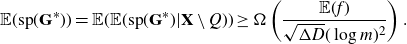
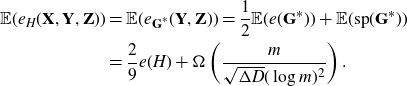 \begin{align*}\mathbb{E}(e_H(\textbf{X},\textbf{Y},\textbf{Z}))&=\mathbb{E}(e_{\textbf{G}^*}(\textbf{Y},\textbf{Z}))=\frac{1}{2}\mathbb{E}(e(\textbf{G}^*))+\mathbb{E}(\mathrm{sp}(\textbf{G}^*))\\&=\frac{2}{9}e(H)+\Omega\left(\frac{m}{\sqrt{\Delta D}(\log m)^2}\right).\end{align*}
Therefore, choosing a partition $(\textbf{X},\textbf{Y},\textbf{Z})$
achieving at least the expectation, we find that
$(\textbf{X},\textbf{Y},\textbf{Z})$
achieving at least the expectation, we find that
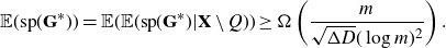
 \begin{align*}\mathrm{sp}_3(H)=\Omega\left(\frac{m}{\sqrt{\Delta D}(\log m)^2}\right).\end{align*}
From this, Theorem 1·2 follows almost immediately. In particular, we prove the following slightly more general result.
Theorem 5·2. Let H be a 3-graph with m edges and maximum co-degree D. Then
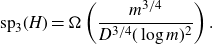 \begin{align*}\mathrm{sp}_3(H)=\Omega\left(\frac{m^{3/4}}{D^{3/4}(\log m)^2}\right).\end{align*}
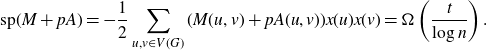
Proof. Let G be the underlying graph of H, then $e(G)=3m$
. Let
$e(G)=3m$
. Let $\Delta=100D^{1/2}m^{1/2}$
, let T be the set of vertices of G of degree more than
$\Delta=100D^{1/2}m^{1/2}$
, let T be the set of vertices of G of degree more than $\Delta$
, and let
$\Delta$
, and let $S=V(G)\setminus T$
. As
$S=V(G)\setminus T$
. As $6m=2e(G)\geq |T|\Delta$
, we get that
$6m=2e(G)\geq |T|\Delta$
, we get that $|T|\leq 0.1m^{1/2}D^{-1/2}$
. Hence, as the multiplicity of every edge of G is at most D, we can write
$|T|\leq 0.1m^{1/2}D^{-1/2}$
. Hence, as the multiplicity of every edge of G is at most D, we can write $e(G[T])\leq ({D}/{2})|T|^2\leq ({1}/{200})m$
.
$e(G[T])\leq ({D}/{2})|T|^2\leq ({1}/{200})m$
.
If $e_G(S,T)\geq 1.6m$
, then
$e_G(S,T)\geq 1.6m$
, then $\mathrm{sp}(G)\geq 0.1 m$
, so we are done as Lemma 2·4 implies
$\mathrm{sp}(G)\geq 0.1 m$
, so we are done as Lemma 2·4 implies $\mathrm{sp}_3(H)\geq ({1}/{12})\mathrm{sp}(G)$
.
$\mathrm{sp}_3(H)\geq ({1}/{12})\mathrm{sp}(G)$
.
Hence, we may assume that $e_G(S,T)\lt 1.6m$
. But then we must have
$e_G(S,T)\lt 1.6m$
. But then we must have $e(G[S])\geq 1.3m$
, as
$e(G[S])\geq 1.3m$
, as $e(G[T])+e_G(S,T)+e(G[S])=e(G)=3m$
. Moreover,
$e(G[T])+e_G(S,T)+e(G[S])=e(G)=3m$
. Moreover,
 \begin{align*}e(G[S])\leq 3e(H[S])+e_H(S,T) = 3e(H[S])+\frac{1}{2}e_G(S,T),\end{align*}
from which we conclude that $e(H[S])\geq 0.1 m$
. The maximum degree of H[S] is less than the maximum degree of G[S], which is less than
$e(H[S])\geq 0.1 m$
. The maximum degree of H[S] is less than the maximum degree of G[S], which is less than $\Delta=100m^{1/2}D^{1/2}$
. Also, the maximum co-degree of H[S] is at most D, so applying Theorem 5·1 to the subhypergraph induced by S finishes the proof.
$\Delta=100m^{1/2}D^{1/2}$
. Also, the maximum co-degree of H[S] is at most D, so applying Theorem 5·1 to the subhypergraph induced by S finishes the proof.
Next, we prove Theorem 1·1.
Proof of Theorem 1·1. Let G be the underlying graph of H, and consider G as an edge weighted graph, where the weight of each edge is its multiplicity. We may assume that $\mathrm{sp}(G)\leq {m^{3/5}}/{(\log m)^2}$
, otherwise we are done by Lemma 2·4. Let
$\mathrm{sp}(G)\leq {m^{3/5}}/{(\log m)^2}$
, otherwise we are done by Lemma 2·4. Let $D=m^{1/5}$
. Say that an edge e of G is D-heavy if its weight is at least D.
$D=m^{1/5}$
. Say that an edge e of G is D-heavy if its weight is at least D.
Let S be the vertex set of a maximal matching of D-heavy edges.
Lemma 5·3. $|S|\lt m^{2/5}$
Proof. Assume that $|S|\geq m^{2/5}$
, and let
$|S|\geq m^{2/5}$
, and let $e_1,\dots,e_s$
be a matching of D-heavy edges, where
$e_1,\dots,e_s$
be a matching of D-heavy edges, where $s=m^{2/5}/2$
. By Lemma 2·5, we have
$s=m^{2/5}/2$
. By Lemma 2·5, we have
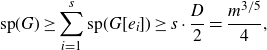 \begin{align*}\mathrm{sp}(G)\geq \sum_{i=1}^{s}\mathrm{sp}(G[e_i])\geq s\cdot \frac{D}{2}=\frac{m^{3/5}}{4},\end{align*}
a contradiction.
Let $\Delta=m^{3/5}$
, and let T be the set of vertices of G of degree more than
$\Delta=m^{3/5}$
, and let T be the set of vertices of G of degree more than $\Delta$
. Then
$\Delta$
. Then $3m=e(G)\geq ({1}/{2})|T|\Delta$
, so
$3m=e(G)\geq ({1}/{2})|T|\Delta$
, so $|T|\leq 6m^{2/5}$
. Let
$|T|\leq 6m^{2/5}$
. Let $U=S\cup T$
, then
$U=S\cup T$
, then $|U|\leq 7m^{2/5}$
.
$|U|\leq 7m^{2/5}$
.
Lemma 5·4. $e(G[U])\leq 0.1m$
Proof. If $e(G[U])\gt 0.1m$
, then by Lemmas 2·5 and 2·3, we get
$e(G[U])\gt 0.1m$
, then by Lemmas 2·5 and 2·3, we get
 \begin{align*}\mathrm{sp}(G)\geq \mathrm{sp}(G[U])= \Omega\left(\frac{e(G[U])}{|U|}\right)=\Omega(m^{3/5}),\end{align*}
a contradiction.
Let $W=U^c$
. Then G[W] contains no D-heavy edges, and the maximum degree of G[W] is at most
$W=U^c$
. Then G[W] contains no D-heavy edges, and the maximum degree of G[W] is at most $\Delta$
. Also,
$\Delta$
. Also, $e_G(U,W)\leq 1.6m$
, as otherwise
$e_G(U,W)\leq 1.6m$
, as otherwise $\mathrm{sp}(G)\geq 0.1m$
. This implies that
$\mathrm{sp}(G)\geq 0.1m$
. This implies that $e_H(U,W)\leq 0.8m$
and that
$e_H(U,W)\leq 0.8m$
and that $e(G[W])=e(G)-e(G[U])-e_G(U,W)\geq 1.3m$
. But then
$e(G[W])=e(G)-e(G[U])-e_G(U,W)\geq 1.3m$
. But then
 \begin{align*}e(H[W])\geq \frac{1}{3}(e(G[W])-e_H(U,W))\gt 0.1m.\end{align*}
Thus, H[W] is an induced subhypergraph of H with at least $0.1m$
edges, maximum degree at most
$0.1m$
edges, maximum degree at most $\Delta$
, and maximum co-degree at most D. Applying Theorem 5·1, we conclude that
$\Delta$
, and maximum co-degree at most D. Applying Theorem 5·1, we conclude that
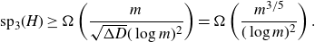 \begin{align*}\mathrm{sp}_3(H)\geq \Omega\left(\frac{m}{\sqrt{\Delta D}(\log m)^2}\right)=\Omega\left(\frac{m^{3/5}}{(\log m)^2}\right).\end{align*}
Finally, we prove Theorem 1·4.
Proof of Theorem 1·4. Let $H_r=H$
, and for
$H_r=H$
, and for $i=r-1,\dots,3$
, let
$i=r-1,\dots,3$
, let $H_i$
be the underlying i-graph of
$H_i$
be the underlying i-graph of $H_{i+1}$
. Then by Lemma 2·6,
$H_{i+1}$
. Then by Lemma 2·6, $\mathrm{sp}_{i+1}(H_{i+1})\geq ({1}/{4(i+1))}\mathrm{sp}_{i}(H_i)$
. From this,
$\mathrm{sp}_{i+1}(H_{i+1})\geq ({1}/{4(i+1))}\mathrm{sp}_{i}(H_i)$
. From this, $\mathrm{sp}_r(H)\geq \Omega_r(\mathrm{sp}_3(H_{3}))$
. But
$\mathrm{sp}_r(H)\geq \Omega_r(\mathrm{sp}_3(H_{3}))$
. But $H_3$
has
$H_3$
has $r(r-1)\dots 4\cdot m$
edges, so
$r(r-1)\dots 4\cdot m$
edges, so $\mathrm{sp}_3(H_3)=\Omega_r ({m^{3/5}}/{(\log m)^2})$
by Theorem 1·1. Thus,
$\mathrm{sp}_3(H_3)=\Omega_r ({m^{3/5}}/{(\log m)^2})$
by Theorem 1·1. Thus, $\mathrm{sp}_r(H)=\Omega_r ({m^{3/5}}/{(\log m)^2})$
as well. Note that we also have
$\mathrm{sp}_r(H)=\Omega_r ({m^{3/5}}/{(\log m)^2})$
as well. Note that we also have $\mathrm{sp}_{r-1}(H_{r-1})=\Omega_r ({m^{3/5}}/{(\log m)^2})$
. Combining this with
$\mathrm{sp}_{r-1}(H_{r-1})=\Omega_r ({m^{3/5}}/{(\log m)^2})$
. Combining this with $\mathrm{sp}_{r-1}(H) \geq ({1}/{2})\mathrm{sp}_{r-1}(H_{r-1})$
guaranteed by Lemma 2·6, we conclude that the statement also holds for
$\mathrm{sp}_{r-1}(H) \geq ({1}/{2})\mathrm{sp}_{r-1}(H_{r-1})$
guaranteed by Lemma 2·6, we conclude that the statement also holds for $k = r-1$
.
$k = r-1$
.
In case H is linear, the maximum co-degree of $H_3$
is
$H_3$
is $O_r(1)$
, so applying Theorem 5·2 gives the desired result.
$O_r(1)$
, so applying Theorem 5·2 gives the desired result.
6. Concluding remarks
In this paper, we proved that every r-graph with m edges contains an r-partite subhypergraph with at least $({r!}/{r^r})m+m^{3/5-o(1)}$
edges. This is still somewhat smaller than the conjectured bound
$({r!}/{r^r})m+m^{3/5-o(1)}$
edges. This is still somewhat smaller than the conjectured bound $({r!}/{r^r})m+\Omega_r(m^{2/3})$
of Conlon, Fox, Kwan and Sudakov [Reference Conlon, Fox, Kwan and Sudakov6]. In order to prove this conjecture, it is enough to prove the following strengthening of Theorem 1·3.
$({r!}/{r^r})m+\Omega_r(m^{2/3})$
of Conlon, Fox, Kwan and Sudakov [Reference Conlon, Fox, Kwan and Sudakov6]. In order to prove this conjecture, it is enough to prove the following strengthening of Theorem 1·3.
Conjecture 6·1. If H is a 3-multigraph that contains an induced subhypergraph with m edges and maximum degree $\Delta$
, then
$\Delta$
, then $\mathrm{sp}_3(H)=\Omega({m}/{\sqrt{\Delta}})$
.
$\mathrm{sp}_3(H)=\Omega({m}/{\sqrt{\Delta}})$
.
Indeed, our Theorem 1·3 is sharp (up to logarithmic terms) as long as the maximum co-degree is O(1). However, we believe the dependence on the co-degree in our lower bound is not necessary. On another note, we are unable to extend our methods to attack the problem of k-cuts in r-graphs in case $k\leq r-2$
. The following remains an intriguing open problem.
$k\leq r-2$
. The following remains an intriguing open problem.
Conjecture 6·2 ([Reference Conlon, Fox, Kwan and Sudakov6]). Let $2\leq k\leq r$
be integers such that
$2\leq k\leq r$
be integers such that $r\geq 3$
and
$r\geq 3$
and $(r,k)\neq (3,2)$
. If H is an r-graph with m edges, then
$(r,k)\neq (3,2)$
. If H is an r-graph with m edges, then $\mathrm{sp}_k(H)=\Omega_r(m^{2/3})$
.
$\mathrm{sp}_k(H)=\Omega_r(m^{2/3})$
.
In the case of linear hypergraphs, we proved that $\mathrm{sp}_r(H)\gt m^{3/4-o(1)}$
, which is optimal up to the o(1) term. It would be interesting to extend this result for k-cuts as well in case
$\mathrm{sp}_r(H)\gt m^{3/4-o(1)}$
, which is optimal up to the o(1) term. It would be interesting to extend this result for k-cuts as well in case $k\leq r-2$
, or to improve the o(1) term.
$k\leq r-2$
, or to improve the o(1) term.
Conjecture 6·3. Let $2\leq k\leq r$
be integers such that
$2\leq k\leq r$
be integers such that $r\geq 3$
and
$r\geq 3$
and $(r,k)\neq (3,2)$
. If H is a linear r-graph with m edges, then
$(r,k)\neq (3,2)$
. If H is a linear r-graph with m edges, then $\mathrm{sp}_k(H)=\Omega_r(m^{3/4})$
.
$\mathrm{sp}_k(H)=\Omega_r(m^{3/4})$
.
Acknowledgments
We would like to thank Klas Markström for pointing out useful matrix concentration inequalities, and the anonymous referee for many useful comments and suggestions. Also, we would like to thank Shengjie Xie and Jie Ma for pointing out a mistake in an earlier version of our paper.

