


1. Introduction
1·1. Symmetric Ramsey properties of random graphs
Given graphs $G$
and
$G$
and $H_1, \dotsc, H_r$
, one says that G is Ramsey for the tuple
$H_1, \dotsc, H_r$
, one says that G is Ramsey for the tuple $(H_1,\dotsc,H_r)$
if, for every r-colouring of the edges of G, there is a monochromatic copy of
$(H_1,\dotsc,H_r)$
if, for every r-colouring of the edges of G, there is a monochromatic copy of $H_i$
in some colour
$H_i$
in some colour $i \in [\![{r}]\!]$
. In the symmetric case
$i \in [\![{r}]\!]$
. In the symmetric case $H_1=\dotsb=H_r=H$
, we simply say that G is Ramsey for H in r colours. Ramsey’s theorem [
Reference Ramsey24
] implies that the complete graph
$H_1=\dotsb=H_r=H$
, we simply say that G is Ramsey for H in r colours. Ramsey’s theorem [
Reference Ramsey24
] implies that the complete graph $K_n$
is Ramsey for
$K_n$
is Ramsey for $(H_1,\dotsc,H_r)$
whenever n is sufficiently large. The fundamental question of graph Ramsey theory is to determine, for a given tuple
$(H_1,\dotsc,H_r)$
whenever n is sufficiently large. The fundamental question of graph Ramsey theory is to determine, for a given tuple $(H_1, \dotsc, H_r)$
, which graphs
$(H_1, \dotsc, H_r)$
, which graphs $G$
are Ramsey for it. For more on this question, as well as the many fascinating sub-questions it contains, we refer the reader to the survey [
Reference Conlon, Fox and Sudakov3
].
$G$
are Ramsey for it. For more on this question, as well as the many fascinating sub-questions it contains, we refer the reader to the survey [
Reference Conlon, Fox and Sudakov3
].
In this paper, we are interested in Ramsey properties of random graphs, a topic that was initiated in the late 1980s by Frankl–Rödl [
Reference Frankl and Rödl6
] and Łuczak–Ruciński–Voigt [
Reference Łuczak, Ruciński and Voigt31
]. The main question in this area is, for a given tuple $(H_1,\dotsc,H_r)$
, which functions
$(H_1,\dotsc,H_r)$
, which functions $p=p(n)$
satisfy that
$p=p(n)$
satisfy that $G_{n,p}$
is Ramsey for
$G_{n,p}$
is Ramsey for $(H_1,\ldots,H_r)$
a.a.s.Footnote 1 In the case
$(H_1,\ldots,H_r)$
a.a.s.Footnote 1 In the case $H_1=\dotsb=H_r$
, this question was resolved in the remarkable work of Rödl and Ruciński [
Reference Rödl and Ruciński25–Reference Rödl and Ruciński27
]. In order to state their result, we need the following terminology and notation. For a graph
$H_1=\dotsb=H_r$
, this question was resolved in the remarkable work of Rödl and Ruciński [
Reference Rödl and Ruciński25–Reference Rödl and Ruciński27
]. In order to state their result, we need the following terminology and notation. For a graph $J$
, we denote by
$J$
, we denote by $v_J$
and
$v_J$
and $e_J$
the number of vertices and edges, respectively, of J. The maximal 2-density of a non-empty graph
$e_J$
the number of vertices and edges, respectively, of J. The maximal 2-density of a non-empty graph $H$
with
$H$
with $v_H \geq 3$
is then definedFootnote 2 to be
$v_H \geq 3$
is then definedFootnote 2 to be
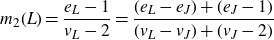
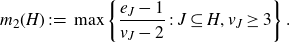 \[ m_2(H) \;:\!=\; \max \left\{ \frac{e_J-1}{v_J-2}\; :\; J \subseteq H, v_J \geq 3\right\}.\]
With this notation, we can state the random Ramsey theorem of Rödl and Ruciński [ Reference Rödl and Ruciński27 ].
Theorem 1·1 (Rödl–Ruciński [
Reference Rödl and Ruciński27
]). For every graph H which is not a forestFootnote 3 and every integer $r \geq 2$
, there exist constants
$r \geq 2$
, there exist constants $c,C>0$
such that
$c,C>0$
such that
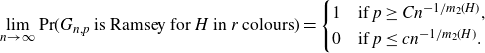 \[ \lim_{n \to \infty}\mathrm{Pr}(G_{n,p}\text{ is Ramsey for} \textit{H}\, \text{in}\, \textit{r} \text{colours}) = \begin{cases} 1&\text{if } p \geq Cn^{-1/m_2(H)},\\ 0&\text{if } p \leq cn^{-1/m_2(H)}. \end{cases} \]
As with many such threshold results for random graph properties, Theorem 1·1 really consists of two statements: the 1-statement, which says that $G_{n,p}$
satisfies the desired property a.a.s. once p is above some threshold, and the 0-statement, which says that
$G_{n,p}$
satisfies the desired property a.a.s. once p is above some threshold, and the 0-statement, which says that $G_{n,p}$
a.a.s. fails to satisfy the desired property if p is below some threshold.
$G_{n,p}$
a.a.s. fails to satisfy the desired property if p is below some threshold.
In recent years, there has been a great deal of work on transferring combinatorial theorems, such as Ramsey’s theorem or Turán’s theorem [ Reference Turán30 ], to sparse random settings. As a consequence, several new proofs of the 1-statement of Theorem 1·1 have been found. Two such proofs were first given by Conlon–Gowers [ Reference Conlon and Gowers4 ] and, independently, by Friedgut–Rödl–Schacht [ Reference Friedgut, Rödl and Schacht8 ] (see also Schacht [ Reference Schacht29 ]) with the use of their transference principles. More recently, Nenadov and Steger [ Reference Nenadov and Steger22 ] found a very short proof of the 1-statement of Theorem 1·1 that uses the hypergraph container method of Saxton–Thomason [ Reference Saxton and Thomason28 ] and Balogh–Morris–Samotij [ Reference Balogh, Morris and Samotij1 ].
Whereas the 0-statement of the aforementioned sparse random analogue of Turán’s theorem is very easy to establish—one simply deletes an arbitrary edge from every copy of H—proving the 0-statement of Theorem 1·1 requires a significant amount of work. Indeed, any proof of the 0-statement of Theorem 1·1 has to argue that, with probability close to one, $G_{n,p}$
does not contain a subgraph G that is Ramsey for H in r colours. As is well known (see e.g. [
Reference Janson, Łuczak and Ruciński14
, Theorem 3·4]), the probability that
$G_{n,p}$
does not contain a subgraph G that is Ramsey for H in r colours. As is well known (see e.g. [
Reference Janson, Łuczak and Ruciński14
, Theorem 3·4]), the probability that $G_{n,p}$
contains G as a subgraph is bounded away from zero if and only if
$G_{n,p}$
contains G as a subgraph is bounded away from zero if and only if $p = \Omega(n^{-1/m(G)})$
, where m(G) is the maximal density of G, defined by
$p = \Omega(n^{-1/m(G)})$
, where m(G) is the maximal density of G, defined by
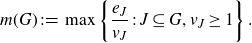 \[ m(G) \;:\!=\; \max \left\{ \frac{e_J}{v_J}\;:\; J\subseteq G, v_J \geq 1\right\}.\]
Therefore, a prerequisite for any proof of the 0-statement is the following result, which (slightly paraphrasing the terms of Rödl and Ruciński [
Reference Rödl and Ruciński27
]) is called the deterministic lemma: if a graph $G$
is Ramsey for H in r colours, then
$G$
is Ramsey for H in r colours, then $m(G) \gt m_2(H)$
. The validity of the deterministic lemma is by no means trivial; in particular, it turns out to be false if we remove the assumption that H is not a forest [
Reference Friedgut and Krivelevich7, Reference Rödl and Ruciński27
], or if we move from graphs to hypergraphs [
Reference Gugelmann, Nenadov, Person, Škorić, Steger and Thomas9
].
$m(G) \gt m_2(H)$
. The validity of the deterministic lemma is by no means trivial; in particular, it turns out to be false if we remove the assumption that H is not a forest [
Reference Friedgut and Krivelevich7, Reference Rödl and Ruciński27
], or if we move from graphs to hypergraphs [
Reference Gugelmann, Nenadov, Person, Škorić, Steger and Thomas9
].
The deterministic lemma only implies that, under the assumption of the 0-statement, $G_{n,p}$
a.a.s. does not contain any bounded sized subgraph that is Ramsey for H. In order to rule out larger Ramsey graphs, one needs additional arguments. Rödl and Ruciński achieve this by a sophisticated union bound argument over a carefully chosen family
$G_{n,p}$
a.a.s. does not contain any bounded sized subgraph that is Ramsey for H. In order to rule out larger Ramsey graphs, one needs additional arguments. Rödl and Ruciński achieve this by a sophisticated union bound argument over a carefully chosen family $\mathcal{S}$
of graphs such that each large minimally-Ramsey graph is guaranteed to contain some
$\mathcal{S}$
of graphs such that each large minimally-Ramsey graph is guaranteed to contain some $S \in \mathcal{S}$
as a subgraph. This part of the proof is encapsulated in the so-called probabilistic lemma, which states that
$S \in \mathcal{S}$
as a subgraph. This part of the proof is encapsulated in the so-called probabilistic lemma, which states that $G_{n,p}$
is not Ramsey for H unless it contains a bounded sized subgraph that is Ramsey for H.
$G_{n,p}$
is not Ramsey for H unless it contains a bounded sized subgraph that is Ramsey for H.
1·2. Asymmetric Ramsey properties of random graphs
Given our good understanding of Ramsey properties of random graphs in the symmetric case, provided by Theorem 1·1, it is natural to ask what happens if we remove the assumption that $H_1=\dotsb=H_r$
. This question was first raised by Kohayakawa and Kreuter [
Reference Kohayakawa and Kreuter15
], who proposed a natural conjecture for the threshold controlling when
$H_1=\dotsb=H_r$
. This question was first raised by Kohayakawa and Kreuter [
Reference Kohayakawa and Kreuter15
], who proposed a natural conjecture for the threshold controlling when $G_{n,p}$
is Ramsey for an arbitrary tuple
$G_{n,p}$
is Ramsey for an arbitrary tuple $(H_1,\dotsc,H_r)$
. To state their conjecture, we need the notion of the mixed 2-density: for graphs
$(H_1,\dotsc,H_r)$
. To state their conjecture, we need the notion of the mixed 2-density: for graphs $H_1,H_2$
with
$H_1,H_2$
with $m_2(H_1) \geq m_2(H_2)$
, their mixed 2-density is defined as
$m_2(H_1) \geq m_2(H_2)$
, their mixed 2-density is defined as
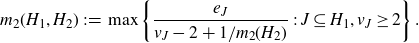 \[ m_2(H_1,H_2) \;:\!=\; \max \left\{ \frac{e_{J}}{v_{J}-2+1/m_2(H_2)} \;:\; J \subseteq H_1, v_J \geq 2 \right\}.\]
With this terminology, we may state the conjecture of Kohayakawa and Kreuter [ Reference Kohayakawa and Kreuter15 ].
Conjecture 1·2 (Kohayakawa–Kreuter [
Reference Kohayakawa and Kreuter15
]). Let $H_1,\ldots,H_r$
be graphs satisfying
$H_1,\ldots,H_r$
be graphs satisfying $m_2(H_1) \geq \dotsb \geq m_2(H_r)$
and
$m_2(H_1) \geq \dotsb \geq m_2(H_r)$
and $m_2(H_2) \gt 1$
. There exist constants
$m_2(H_2) \gt 1$
. There exist constants $c,C>0$
such that
$c,C>0$
such that
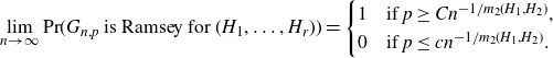 \[ \lim_{n \to \infty}\mathrm{Pr}(G_{n,p}\text{ is Ramsey for } (H_1,\dotsc,H_r)) = \begin{cases} 1&\text{if }p \geq Cn^{-1/m_2(H_1,H_2)},\\ 0&\text{if }p \leq cn^{-1/m_2(H_1,H_2)}. \end{cases} \]
The assumption $m_2(H_2) \gt 1$
is equivalent to requiring that
$m_2(H_2) \gt 1$
is equivalent to requiring that $H_1$
and
$H_1$
and $H_2$
are not forests; it was added by Kohayakawa, Schacht, and Spöhel [
Reference Kohayakawa, Schacht and Spöhel16
] to rule out sporadic counterexamples, in analogy with the assumption that H is not a forest in Theorem 1·1.
$H_2$
are not forests; it was added by Kohayakawa, Schacht, and Spöhel [
Reference Kohayakawa, Schacht and Spöhel16
] to rule out sporadic counterexamples, in analogy with the assumption that H is not a forest in Theorem 1·1.
The role of the mixed 2-density $m_2(H_1, H_2)$
in the context of Conjecture 1·2 can seem a little mysterious at first, but there is a natural (heuristic) explanation. Since one can colour all edges that do not lie in a copy of
$m_2(H_1, H_2)$
in the context of Conjecture 1·2 can seem a little mysterious at first, but there is a natural (heuristic) explanation. Since one can colour all edges that do not lie in a copy of $H_1$
with colour 1, the only important edges are those that do lie in copies of
$H_1$
with colour 1, the only important edges are those that do lie in copies of $H_1$
. The mixed 2-density is defined in such a way that
$H_1$
. The mixed 2-density is defined in such a way that $p =\Theta(n^{-1/m_2(H_1,H_2)})$
is the threshold at which the number of copies of (the densest subgraph of) each of
$p =\Theta(n^{-1/m_2(H_1,H_2)})$
is the threshold at which the number of copies of (the densest subgraph of) each of $H_2, \dotsc, H_r$
is at least of the same order of magnitude as the number of edges in the union of all copies of (the densest subgraph of)
$H_2, \dotsc, H_r$
is at least of the same order of magnitude as the number of edges in the union of all copies of (the densest subgraph of) $H_1$
in
$H_1$
in $G_{n,p}$
. Since at least one edge in each copy of
$G_{n,p}$
. Since at least one edge in each copy of $H_1$
must receive a colour from
$H_1$
must receive a colour from $\{2, \dotsc, r\}$
, this is the point where avoiding monochromatic copies of
$\{2, \dotsc, r\}$
, this is the point where avoiding monochromatic copies of $H_2, \dotsc, H_r$
becomes difficult.
$H_2, \dotsc, H_r$
becomes difficult.
Conjecture 1·2 has received a great deal of attention over the years, and has been proved in a number of special cases. Following a sequence of partial results [ Reference Gugelmann, Nenadov, Person, Škorić, Steger and Thomas9, Reference Hancock, Staden and Treglown11, Reference Kohayakawa and Kreuter15, Reference Kohayakawa, Schacht and Spöhel16, Reference Marciniszyn, Skokan, Spöhel and Steger19 ], the 1-statement of Conjecture 1·2 was proved by Mousset, Nenadov and Samotij [ Reference Mousset, Nenadov and Samotij20 ] with the use of the container method as well as a randomised “typing” procedure. We henceforth focus on the 0-statement, where progress has been more limited.
Note that, in order to prove the 0-statement, one can make several simplifying assumptions. First, one can assume that r, the number of colours, is equal to 2. Indeed, if one can a.a.s. 2-colour the edges of $G_{n,p}$
and avoid monochromatic copies of
$G_{n,p}$
and avoid monochromatic copies of $H_1,H_2$
in colours 1,2, respectively, then certainly
$H_1,H_2$
in colours 1,2, respectively, then certainly $G_{n,p}$
is not Ramsey for
$G_{n,p}$
is not Ramsey for $(H_1,\ldots,H_r)$
. Furthermore, if
$(H_1,\ldots,H_r)$
. Furthermore, if $H_2' \subseteq H_2$
is a subgraph satisfying
$H_2' \subseteq H_2$
is a subgraph satisfying $m_2(H_2')=m_2(H_2)$
, then the 0-statement for the pair
$m_2(H_2')=m_2(H_2)$
, then the 0-statement for the pair $(H_1,H_2')$
implies the 0-statement for
$(H_1,H_2')$
implies the 0-statement for $(H_1,H_2)$
, as any colouring with no monochromatic copy of
$(H_1,H_2)$
, as any colouring with no monochromatic copy of $H_2'$
in particular has no monochromatic copy of
$H_2'$
in particular has no monochromatic copy of $H_2$
. Thus, we may assume that
$H_2$
. Thus, we may assume that $H_2$
is strictly 2-balanced, meaning that
$H_2$
is strictly 2-balanced, meaning that $m_2(H_2') \lt m_2(H_2)$
for any
$m_2(H_2') \lt m_2(H_2)$
for any $H_2' \subsetneq H_2$
. For exactly the same reason, we may assume that
$H_2' \subsetneq H_2$
. For exactly the same reason, we may assume that $H_1$
is strictly
$H_1$
is strictly $m_2(\cdot,H_2)$
-balanced, meaning that
$m_2(\cdot,H_2)$
-balanced, meaning that $m_2(H_1',H_2)\lt m_2(H_1,H_2)$
for any
$m_2(H_1',H_2)\lt m_2(H_1,H_2)$
for any $H_1' \subsetneq H_1$
. Let us say that the pair
$H_1' \subsetneq H_1$
. Let us say that the pair $(H_1,H_2)$
is strictly balanced if
$(H_1,H_2)$
is strictly balanced if $H_2$
is strictly 2-balanced and
$H_2$
is strictly 2-balanced and $H_1$
is strictly
$H_1$
is strictly $m_2(\cdot,H_2)$
-balanced. Additionally, let us say that
$m_2(\cdot,H_2)$
-balanced. Additionally, let us say that $(H_1',H_2')$
is a strictly balanced pair of subgraphs of
$(H_1',H_2')$
is a strictly balanced pair of subgraphs of $(H_1,H_2)$
if
$(H_1,H_2)$
if $(H_1',H_2')$
is strictly balanced and satisfies
$(H_1',H_2')$
is strictly balanced and satisfies $m_2(H_2')=m_2(H_2)$
and
$m_2(H_2')=m_2(H_2)$
and $m_2(H_1',H_2')=m_2(H_1,H_2)$
. All previous works on the 0-statement of Conjecture 1·2 have made these simplifying assumptions, working in the case
$m_2(H_1',H_2')=m_2(H_1,H_2)$
. All previous works on the 0-statement of Conjecture 1·2 have made these simplifying assumptions, working in the case $r=2$
and with a strictly balanced pair
$r=2$
and with a strictly balanced pair $(H_1,H_2)$
.
$(H_1,H_2)$
.
The original paper of Kohayakawa and Kreuter [
Reference Kohayakawa and Kreuter15
] proved the 0-statement of Conjecture 1·2 when $H_1$
and
$H_1$
and $H_2$
are cycles. This was extended to the case when both
$H_2$
are cycles. This was extended to the case when both $H_1$
and
$H_1$
and $H_2$
are cliques in [
Reference Marciniszyn, Skokan, Spöhel and Steger19
], and to the case when
$H_2$
are cliques in [
Reference Marciniszyn, Skokan, Spöhel and Steger19
], and to the case when $H_1$
is a clique and
$H_1$
is a clique and $H_2$
is a cycle in [
Reference Liebenau, Mattos, Mendonça and Skokan18
]. To date, the most general result is due to Hyde [
Reference Hyde13
], who proved the 0-statement of Conjecture 1·2 for almost all pairs of regular graphs
$H_2$
is a cycle in [
Reference Liebenau, Mattos, Mendonça and Skokan18
]. To date, the most general result is due to Hyde [
Reference Hyde13
], who proved the 0-statement of Conjecture 1·2 for almost all pairs of regular graphs $(H_1,H_2)$
; in fact, this follows from Hyde’s main result [
Reference Hyde13
, Theorem 1·9], which establishes a certain deterministic condition whose validity implies the 0-statement of Conjecture 1·2. Finally, the first two authors [
Reference Kuperwasser and Samotij17
] recently proved the 0-statement of Conjecture 1·2 in the case where
$(H_1,H_2)$
; in fact, this follows from Hyde’s main result [
Reference Hyde13
, Theorem 1·9], which establishes a certain deterministic condition whose validity implies the 0-statement of Conjecture 1·2. Finally, the first two authors [
Reference Kuperwasser and Samotij17
] recently proved the 0-statement of Conjecture 1·2 in the case where $m_2(H_1)=m_2(H_2)$
. Because of this, we henceforth focus on the case that
$m_2(H_1)=m_2(H_2)$
. Because of this, we henceforth focus on the case that $m_2(H_1)>m_2(H_2)$
.
$m_2(H_1)>m_2(H_2)$
.
1·3. New results
As in the symmetric setting, a necessary prerequisite for proving the 0-statement of Conjecture 1·2 is proving the following deterministic lemma: if G is Ramsey for $(H_1,H_2)$
, then
$(H_1,H_2)$
, then $m(G) \gt m_2(H_1,H_2)$
. The main result in this paper is a corresponding probabilistic lemma, which states that this obvious necessary condition is also sufficient.
$m(G) \gt m_2(H_1,H_2)$
. The main result in this paper is a corresponding probabilistic lemma, which states that this obvious necessary condition is also sufficient.
Theorem 1·3. The 0-statement of Conjecture 1·2 holds if and only if, for every strictly balanced pair $(H_1,H_2)$
, every graph G that is Ramsey for
$(H_1,H_2)$
, every graph G that is Ramsey for $(H_1, H_2)$
satisfies
$(H_1, H_2)$
satisfies $m(G) \gt m_2(H_1, H_2)$
.
$m(G) \gt m_2(H_1, H_2)$
.
More precisely, we prove that if $(H_1,H_2)$
is any pair of graphs and
$(H_1,H_2)$
is any pair of graphs and $(H_1',H_2')$
is a strictly balanced pair of subgraphs of
$(H_1',H_2')$
is a strictly balanced pair of subgraphs of $(H_1,H_2)$
, then the 0-statement of Conjecture 1·2 holds for
$(H_1,H_2)$
, then the 0-statement of Conjecture 1·2 holds for $(H_1,H_2)$
if every graph
$(H_1,H_2)$
if every graph $G$
which is Ramsey for
$G$
which is Ramsey for $(H_1',H_2')$
satisfies
$(H_1',H_2')$
satisfies $m(G) \gt m_2(H_1',H_2') = m_2(H_1,H_2)$
.
$m(G) \gt m_2(H_1',H_2') = m_2(H_1,H_2)$
.
While we believe that the probabilistic lemma, Theorem 1·3, is our main contribution, we are able to prove the deterministic lemma in a wide range of cases. This implies that the 0-statement of Conjecture 1·2 is true for almost all pairs of graphs. The most general statement we can prove is slightly tricky to state because of the necessity of passing to a strictly balanced pair of subgraphs; however, here is a representative example of our results, which avoids this technicality and still implies Conjecture 1·2 for all pairs of sufficiently dense graphs. We state the more general result in Theorem 1·7 below.
Theorem 1·4. Conjecture 1·2 holds for all sequences $H_1,\ldots,H_r$
of graphs satisfying
$H_1,\ldots,H_r$
of graphs satisfying $m_2(H_1) \geq \dotsb \geq m_2(H_r)$
and
$m_2(H_1) \geq \dotsb \geq m_2(H_r)$
and $m_2(H_2) \gt {11}/5$
.
$m_2(H_2) \gt {11}/5$
.
As discussed above, Theorem 1·4 follows easily from Theorem 1·3 and a deterministic lemma for strictly balanced pairs $(H_1,H_2)$
satisfying
$(H_1,H_2)$
satisfying $m_2(H_1) \geq m_2(H_2) \gt {11}/5$
. The deterministic lemma in this setting is actually very straightforward and follows from standard colouring techniques.
$m_2(H_1) \geq m_2(H_2) \gt {11}/5$
. The deterministic lemma in this setting is actually very straightforward and follows from standard colouring techniques.
Using a number of other colouring techniques, we can prove the deterministic lemma (and thus Conjecture 1·2) in several additional cases, which we discuss below. However, let us first propose a conjecture, which we believe to be of independent interest, and whose resolution would immediately imply Conjecture 1·2 in all cases.
Conjecture 1·5. For any graph $G$
, there exists a forest
$G$
, there exists a forest $F \subseteq G$
such that
$F \subseteq G$
such that
 \[ m_2(G \setminus F) \leq m(G). \]
Here, $G \setminus F$
denotes the graph obtained from G by deleting the edges of F (but not deleting any vertices). To give some intuition for Conjecture 1·5, we note that
$G \setminus F$
denotes the graph obtained from G by deleting the edges of F (but not deleting any vertices). To give some intuition for Conjecture 1·5, we note that $m(G) \leq m_2(G) \leq m(G) +1$
for any graph G, and that
$m(G) \leq m_2(G) \leq m(G) +1$
for any graph G, and that $m_2(F)=1$
for any forest F which is not a matching. Thus, it is natural to expect that by deleting the edges of a forest, we could decrease
$m_2(F)=1$
for any forest F which is not a matching. Thus, it is natural to expect that by deleting the edges of a forest, we could decrease $m_2(G)$
by roughly 1. Conjecture 1·5 says that this is roughly the case, in that the deletion of an appropriately-chosen forest can decrease
$m_2(G)$
by roughly 1. Conjecture 1·5 says that this is roughly the case, in that the deletion of an appropriately-chosen forest can decrease $m_2(G)$
to lie below m(G).
$m_2(G)$
to lie below m(G).
Moreover, we note that Conjecture 1·5 easily implies the deterministic lemma in all casesFootnote 4 with $m_2(H_1)>m_2(H_2)$
, and thus implies Conjecture 1·2. Indeed, it is straightforward to verify in this case that
$m_2(H_1)>m_2(H_2)$
, and thus implies Conjecture 1·2. Indeed, it is straightforward to verify in this case that $m_2(H_1) \gt m_2(H_1,H_2)$
(see Lemma 3·4 below). Now, suppose that G is some graph with
$m_2(H_1) \gt m_2(H_1,H_2)$
(see Lemma 3·4 below). Now, suppose that G is some graph with $m(G) \leq m_2(H_1,H_2) \lt m_2(H_1)$
. If Conjecture 1·5 is true, we may partition the edges of G into a forest F and a graph
$m(G) \leq m_2(H_1,H_2) \lt m_2(H_1)$
. If Conjecture 1·5 is true, we may partition the edges of G into a forest F and a graph $K$
with
$K$
with $m_2(K) \leq m(G) \lt m_2(H_1)$
. This latter condition implies, in particular, that K contains no copy of
$m_2(K) \leq m(G) \lt m_2(H_1)$
. This latter condition implies, in particular, that K contains no copy of $H_1$
. Additionally, by the assumption
$H_1$
. Additionally, by the assumption $m_2(H_2) \gt 1$
in Conjecture 1·2, we know that
$m_2(H_2) \gt 1$
in Conjecture 1·2, we know that $H_2$
contains a cycle and thus F contains no copy of
$H_2$
contains a cycle and thus F contains no copy of $H_2$
. In other words, colouring the edges of K with colour 1 and the edges of F with colour 2 witnesses that G is not Ramsey for
$H_2$
. In other words, colouring the edges of K with colour 1 and the edges of F with colour 2 witnesses that G is not Ramsey for $(H_1,\ldots,H_r)$
.
$(H_1,\ldots,H_r)$
.
Because of this, it would be of great interest to prove Conjecture 1·5. Somewhat surprisingly, we know how to prove Conjecture 1·5 under the extra assumption that m(G) is an integer. This extra condition seems fairly artificial, but we do not know how to remove it—our technique uses tools from matroid theory that seem to break down once m(G) is no longer an integer. We present this proof in Appendix B, in the hope that it may serve as a first step to the full resolution of Conjecture 1·5, and thus Conjecture 1·2.
Although we are not able to resolve Conjecture 1·5, we do have a number of other techniques for proving the deterministic lemma, and thus Conjecture 1·2, under certain assumptions. First, we are able to resolve the case when the number of colours is at least three and $m_2(H_2)=m_2(H_3)$
.
$m_2(H_2)=m_2(H_3)$
.
Theorem 1·6. Let $H_1,\ldots,H_r$
be a sequence of graphs with
$H_1,\ldots,H_r$
be a sequence of graphs with $r \geq 3$
and suppose that
$r \geq 3$
and suppose that $m_2(H_1) \geq m_2(H_2) = m_2(H_3) \geq \dotsb \geq m_2(H_r)$
and
$m_2(H_1) \geq m_2(H_2) = m_2(H_3) \geq \dotsb \geq m_2(H_r)$
and $m_2(H_2)>1$
. Then Conjecture 1·2 holds for
$m_2(H_2)>1$
. Then Conjecture 1·2 holds for $H_1,\ldots,H_r$
.
$H_1,\ldots,H_r$
.
We can also prove Conjecture 1·2 in a number of additional cases, expressed in terms of the properties of (a strictly balanced pair of subgraphs of) the pair $(H_1, H_2)$
of two densest graphs.
$(H_1, H_2)$
of two densest graphs.
Recall that the degeneracy of H is the maximum over all $J \subseteq H$
of the minimum degree of J.
$J \subseteq H$
of the minimum degree of J.
Theorem 1·7. Suppose that $(H_1,H_2)$
is strictly balanced. Suppose additionally that one of the following conditions holds:
$(H_1,H_2)$
is strictly balanced. Suppose additionally that one of the following conditions holds:
-
(a) $\chi(H_2) \geq 3$
, or
$\chi(H_2) \geq 3$
, or -
(b)
$H_2$
is not the union of two forests, or -
(c)
$\chi(H_1) \gt m_2(H_1,H_2)+1$
, or -
(d)
$H_1$
has degeneracy at least
$\lfloor 2m_2(H_1,H_2) \rfloor$
, or -
(e)
$H_1=K_{s,t}$
for some
$s,t\geq 2$
, or -
(f)
$m_2(H_1)>\lceil m_2(H_1,H_2) \rceil$
.


In any of these cases, Conjecture 1·2 holds for $(H_1,H_2)$
.
$(H_1,H_2)$
.
Remark. The only graphs $H_2$
which do not satisfy (a) or (b) are sparse bipartite graphs, such as even cycles. On the other hand, (c) applies whenever
$H_2$
which do not satisfy (a) or (b) are sparse bipartite graphs, such as even cycles. On the other hand, (c) applies whenever $H_1$
is a cliqueFootnote 5 or, more generally, a graph obtained from a clique by deleting few edges. Moreover, (d) applies to reasonably dense graphs, as well as all d-regular bipartite graphs with
$H_1$
is a cliqueFootnote 5 or, more generally, a graph obtained from a clique by deleting few edges. Moreover, (d) applies to reasonably dense graphs, as well as all d-regular bipartite graphs with $d \geq 2$
, and (e) handles all cases when
$d \geq 2$
, and (e) handles all cases when $H_1$
is a bicliqueFootnote 6. Thus, very roughly speaking, the strictly balanced cases that remain open in Conjecture 1·2 are those in which
$H_1$
is a bicliqueFootnote 6. Thus, very roughly speaking, the strictly balanced cases that remain open in Conjecture 1·2 are those in which $H_2$
is bipartite and very sparse and
$H_2$
is bipartite and very sparse and $H_1$
is not “too dense”.
$H_1$
is not “too dense”.
Case (f) is somewhat stranger and it is not obvious that there exist graphs to which it applies. However, one can check that, for example, it applies if $H_1 = K_{3,3,3,3}$
and
$H_1 = K_{3,3,3,3}$
and $H_2=C_8$
, and that none of the other cases of Theorem 1·7 (or any of the earlier results on Conjecture 1·2) apply in this case. However, the main reason we include (f) is that it is implied by our partial progress on Conjecture 1·5; since we believe that this conjecture is the correct approach to settling Conjecture 1·2 in its entirety, we wanted to highlight (f).
$H_2=C_8$
, and that none of the other cases of Theorem 1·7 (or any of the earlier results on Conjecture 1·2) apply in this case. However, the main reason we include (f) is that it is implied by our partial progress on Conjecture 1·5; since we believe that this conjecture is the correct approach to settling Conjecture 1·2 in its entirety, we wanted to highlight (f).
We remark that, unfortunately, the conditions in Theorem 1·7 do not exhaust all cases. While it is quite likely that simple additional arguments could resolve further cases, Conjecture 1·5 remains the only (conjectural) approach we have found to resolve Conjecture 1·2 in all cases. Moreover, our proof of the probabilistic lemma implies that, in order to prove Conjecture 1·2 for a pair $(H_1,H_2)$
, it is enough to prove the deterministic lemma for graphs
$(H_1,H_2)$
, it is enough to prove the deterministic lemma for graphs $G$
of order not exceeding an explicit constant
$G$
of order not exceeding an explicit constant $K=K(H_1,H_2)$
. In particular, the validity of Conjecture 1·2 for any specific pair of graphs reduces to a finite computation.
$K=K(H_1,H_2)$
. In particular, the validity of Conjecture 1·2 for any specific pair of graphs reduces to a finite computation.
1·4. Ramsey properties of graph families
All of the results discussed in the previous subsection hold in greater generality, when we replace $H_1,\ldots,H_r$
with r finite families of graphs. In addition to being interesting in its own right, such a generalisation also has important consequences in the original setting of Conjecture 1·2; indeed, our proof of the three-colour result, Theorem 1·6, colours, relies on our ability to work with graph families. Before we state our more general results, we need the following definitions.
$H_1,\ldots,H_r$
with r finite families of graphs. In addition to being interesting in its own right, such a generalisation also has important consequences in the original setting of Conjecture 1·2; indeed, our proof of the three-colour result, Theorem 1·6, colours, relies on our ability to work with graph families. Before we state our more general results, we need the following definitions.
Definition 1·8. Let $\mathcal{H}_1,\ldots,\mathcal{H}_r$
be finite families of graphs. We say that a graph G is Ramsey for
$\mathcal{H}_1,\ldots,\mathcal{H}_r$
be finite families of graphs. We say that a graph G is Ramsey for $(\mathcal{H}_1,\ldots,\mathcal{H}_r)$
if every r-colouring of E(G) contains a monochromatic copy of some
$(\mathcal{H}_1,\ldots,\mathcal{H}_r)$
if every r-colouring of E(G) contains a monochromatic copy of some $H_i \in \mathcal{H}_i$
in some colour
$H_i \in \mathcal{H}_i$
in some colour $i \in [\![{r}]\!]$
.
$i \in [\![{r}]\!]$
.
We now define the appropriate generalizations of the notions of maximum 2-density and mixed 2-density to families of graphs. First, given a finite family of graphs $\mathcal{H}$
, we let
$\mathcal{H}$
, we let
 \[ m_2(\mathcal{H}) \;:\!=\; \min_{H \in \mathcal{H}} m_2(H).\]
Second, given a graph $H$
and a (finite) family
$H$
and a (finite) family $\mathcal{L}$
of graphs, we let
$\mathcal{L}$
of graphs, we let
 \[ m_2(H, \mathcal{L}) \;:\!=\; \max \left\{ \frac{e_{J}}{v_{J}-2+1/m_2(\mathcal{L})} \;:\; J \subseteq H, v_J \geq 2 \right\}.\]
Third, given two finite families of graphs $\mathcal{H}$
and
$\mathcal{H}$
and $\mathcal{L}$
with
$\mathcal{L}$
with $m_2(\mathcal{H}) \geq m_2(\mathcal{L})$
, we define
$m_2(\mathcal{H}) \geq m_2(\mathcal{L})$
, we define
 \[ m_2(\mathcal{H},\mathcal{L}) \;:\!=\; \min_{H \in \mathcal{H}} m_2(H, \mathcal{L}).\]
Finally, continuing the terminology above, let us say that the pair $(\mathcal{H},\mathcal{L})$
is strictly balanced if every graph in
$(\mathcal{H},\mathcal{L})$
is strictly balanced if every graph in $\mathcal{L}$
is strictly 2-balanced and every graph in
$\mathcal{L}$
is strictly 2-balanced and every graph in $\mathcal{H}$
is strictly
$\mathcal{H}$
is strictly $m_2(\cdot,\mathcal{L})$
-balanced.
$m_2(\cdot,\mathcal{L})$
-balanced.
The following conjecture is a natural generalization of Conjecture 1·2 to families of graphs.
Conjecture 1·9 (Kohayakawa–Kreuter conjecture for families). Let $\mathcal{H}_1,\ldots,\mathcal{H}_r$
be finite families of graphs with
$\mathcal{H}_1,\ldots,\mathcal{H}_r$
be finite families of graphs with $m_2(\mathcal{H}_1) \geq \dotsb \geq m_2(\mathcal{H}_r)$
and suppose that
$m_2(\mathcal{H}_1) \geq \dotsb \geq m_2(\mathcal{H}_r)$
and suppose that $m_2(\mathcal{H}_2) \gt 1$
. There exist constants
$m_2(\mathcal{H}_2) \gt 1$
. There exist constants $c,C>0$
such that
$c,C>0$
such that
 \[ \lim_{n \to \infty}\mathrm{Pr}(G_{n,p}\text{ is Ramsey for } (\mathcal{H}_1,\ldots,\mathcal{H}_r)) = \begin{cases} 1&\text{if }p \geq Cn^{-1/m_2(\mathcal{H}_1,\mathcal{H}_2)},\\ 0&\text{if }p \leq cn^{-1/m_2(\mathcal{H}_1,\mathcal{H}_2)}. \end{cases} \]
Note that, for any $H_1 \in \mathcal{H}_1,\ldots,H_r \in \mathcal{H}_r$
, the property of being Ramsey for
$H_1 \in \mathcal{H}_1,\ldots,H_r \in \mathcal{H}_r$
, the property of being Ramsey for $(H_1,\ldots,H_r)$
implies the property of being Ramsey for
$(H_1,\ldots,H_r)$
implies the property of being Ramsey for $(\mathcal{H}_1,\ldots,\mathcal{H}_r)$
. Therefore, the 1-statement of Conjecture 1·9 follows from the 1-statement of Conjecture 1·2, which we know to be true by the result of Mousset, Nenadov, and Samotij [
Reference Mousset, Nenadov and Samotij20
].
$(\mathcal{H}_1,\ldots,\mathcal{H}_r)$
. Therefore, the 1-statement of Conjecture 1·9 follows from the 1-statement of Conjecture 1·2, which we know to be true by the result of Mousset, Nenadov, and Samotij [
Reference Mousset, Nenadov and Samotij20
].
The 0-statement of Conjecture 1·9 remains open; the only progress to date is due to the first two authors [
Reference Kuperwasser and Samotij17
], who proved Conjecture 1·9 whenever $m_2(\mathcal{H}_1)=m_2(\mathcal{H}_2)$
. We make further progress on this conjecture: as in the case of single graphs, we prove a probabilistic lemma that reduces the 0-statement to a deterministic lemma, which is clearly a necessary condition.
$m_2(\mathcal{H}_1)=m_2(\mathcal{H}_2)$
. We make further progress on this conjecture: as in the case of single graphs, we prove a probabilistic lemma that reduces the 0-statement to a deterministic lemma, which is clearly a necessary condition.
Theorem 1·10 (Probabilistic lemma for families). The 0-statement of Conjecture 1·9 holds if and only if, for every strictly balanced pair $(\mathcal{H}_1,\mathcal{H}_2)$
of finite families of graphs, every graph G that is Ramsey for
$(\mathcal{H}_1,\mathcal{H}_2)$
of finite families of graphs, every graph G that is Ramsey for $(\mathcal{H}_1,\mathcal{H}_2)$
satisfies
$(\mathcal{H}_1,\mathcal{H}_2)$
satisfies $m(G) \gt m_2(\mathcal{H}_1,\mathcal{H}_2)$
.
$m(G) \gt m_2(\mathcal{H}_1,\mathcal{H}_2)$
.
As in Theorems 1·4 and 1·7, we can prove the deterministic lemma for families in a wide variety of cases, namely when every graph $H_1 \in \mathcal{H}_1$
or every graph
$H_1 \in \mathcal{H}_1$
or every graph $H_2 \in \mathcal{H}_2$
satisfies one of the conditions in Theorem 1·7. In particular, we resolve Conjecture 1·9 in many cases. However, we believe that the right way to resolve Conjecture 1·9 in its entirety is the same as the right way to resolve the original Kohayakawa–Kreuter conjecture, Conjecture 1·2. Namely, if Conjecture 1·5 is true, then Conjecture 1·9 is true for all families of graphs.
$H_2 \in \mathcal{H}_2$
satisfies one of the conditions in Theorem 1·7. In particular, we resolve Conjecture 1·9 in many cases. However, we believe that the right way to resolve Conjecture 1·9 in its entirety is the same as the right way to resolve the original Kohayakawa–Kreuter conjecture, Conjecture 1·2. Namely, if Conjecture 1·5 is true, then Conjecture 1·9 is true for all families of graphs.
1·5. Organisation
Most of the rest of this paper is dedicated to proving Theorem 1·10 and thus also Theorem 1·3. Our technique is inspired by recent work of the first two authors [
Reference Kuperwasser and Samotij17
], who proved Conjecture 1·9 in the case $m_2(\mathcal{H}_1)=m_2(\mathcal{H}_2)$
. Therefore, we assume henceforth that
$m_2(\mathcal{H}_1)=m_2(\mathcal{H}_2)$
. Therefore, we assume henceforth that $m_2(\mathcal{H}_1)>m_2(\mathcal{H}_2)$
. We will now change notation and denote
$m_2(\mathcal{H}_1)>m_2(\mathcal{H}_2)$
. We will now change notation and denote $\mathcal{H}_1=\mathcal{H}$
and
$\mathcal{H}_1=\mathcal{H}$
and $\mathcal{H}_2=\mathcal{L}$
. The names stand for heavy and light, respectively, and are meant to remind the reader that
$\mathcal{H}_2=\mathcal{L}$
. The names stand for heavy and light, respectively, and are meant to remind the reader that $m_2(\mathcal{L}) \lt m_2(\mathcal{H})$
. We also assume henceforth that
$m_2(\mathcal{L}) \lt m_2(\mathcal{H})$
. We also assume henceforth that $(\mathcal{H},\mathcal{L})$
is a strictly balanced pair of families.
$(\mathcal{H},\mathcal{L})$
is a strictly balanced pair of families.
The rest of this paper is organised as follows. In Section 2, we present a high-level overview of our proof of Theorem 1·10. Section 3 contains a number of preliminaries for the proof, including the definitions and basic properties of cores—a fundamental notion in our approach—as well as several simple numerical lemmas. The proof of Theorem 1·10 is carried out in detail in Section 4. In Section 5, we prove the deterministic lemma under various assumptions, which yields Theorems 1·4 and 1·7 as well as their generalisations to families. We conclude with two appendices: Appendix A proves Theorem 1·6 by explaining what in our proof needs to be adapted to deal with the three-colour setting; and Appendix B presents our partial progress on Conjecture 1·5.
Additional note
As this paper was being written, we learned that very similar results were obtained independently by Bowtell, Hancock and Hyde [ Reference Bowtell, Hancock and Hyde2 ], who also resolve Conjecture 1·2 in the vast majority of cases. As with this paper, they first prove a probabilistic lemma, showing that resolving the Kohayakawa–Kreuter conjecture is equivalent to proving a deterministic colouring result. By using a wider array of colouring techniques, they are able to prove more cases of Conjecture 1·2 than we can. Additionally, they consider a natural generalisation of the Kohayakawa–Kreuter to uniform hypergraphs (a topic that we chose not to pursue here) and establish its 0-statement for almost all pairs of hypergraphs; see also [ Reference Gugelmann, Nenadov, Person, Škorić, Steger and Thomas9 ] for more on such hypergraph questions. In contrast, their work does not cover families of graphs, a generalization that falls out naturally from our approach.
2. Proof outline
We now sketch, at a very high level, the proof of the probabilistic lemma. Let us fix a strictly balanced pair of families $(\mathcal{H},\mathcal{L})$
. We wish to upper-bound the probability that
$(\mathcal{H},\mathcal{L})$
. We wish to upper-bound the probability that $G_{n,p}$
is Ramsey for
$G_{n,p}$
is Ramsey for $(\mathcal{H},\mathcal{L})$
, where
$(\mathcal{H},\mathcal{L})$
, where $p \leq cn^{-1/m_2(\mathcal{H},\mathcal{L})}$
for an appropriately chosen constant
$p \leq cn^{-1/m_2(\mathcal{H},\mathcal{L})}$
for an appropriately chosen constant $c=c(\mathcal{H},\mathcal{L})>0$
. Our approach is modeled on the recent proof of the 0-statement of Theorem 1·1 due to the first two authors [
Reference Kuperwasser and Samotij17
]; however, there are substantial additional difficulties that arise in the asymmetric setting.
$c=c(\mathcal{H},\mathcal{L})>0$
. Our approach is modeled on the recent proof of the 0-statement of Theorem 1·1 due to the first two authors [
Reference Kuperwasser and Samotij17
]; however, there are substantial additional difficulties that arise in the asymmetric setting.
One can immediately make several simplifying assumptions. First, if $G_{n,p}$
is Ramsey for
$G_{n,p}$
is Ramsey for $(\mathcal{H},\mathcal{L})$
, then there exists some
$(\mathcal{H},\mathcal{L})$
, then there exists some $G \subseteq G_{n,p}$
that is minimally Ramsey for
$G \subseteq G_{n,p}$
that is minimally Ramsey for $(\mathcal{H},\mathcal{L})$
, in the sense that any proper subgraph
$(\mathcal{H},\mathcal{L})$
, in the sense that any proper subgraph $G' \subsetneq G$
is not Ramsey for
$G' \subsetneq G$
is not Ramsey for $(\mathcal{H},\mathcal{L})$
. It is not hard to show (see Lemma 3·2 below) that every minimally Ramsey graph has a number of interesting properties. In particular, if G is minimally Ramsey, then every edge of G lies in at least one copy of some
$(\mathcal{H},\mathcal{L})$
. It is not hard to show (see Lemma 3·2 below) that every minimally Ramsey graph has a number of interesting properties. In particular, if G is minimally Ramsey, then every edge of G lies in at least one copy of some $H \in \mathcal{H}$
, and at least one copy of some
$H \in \mathcal{H}$
, and at least one copy of some $L\in \mathcal{L}$
. Our arguments will exploit a well-known strengthening of this property, which we call supporting a core; see Definition 3·1 for the precise definition.
$L\in \mathcal{L}$
. Our arguments will exploit a well-known strengthening of this property, which we call supporting a core; see Definition 3·1 for the precise definition.
We would ideally like to union-bound over all possible minimally Ramsey graphs $G$
in order to show that a.a.s. none of them appears in
$G$
in order to show that a.a.s. none of them appears in $G_{n,p}$
. Unfortunately, there are potentially too many minimally Ramsey graphs for this to be possible. To overcome this, we construct a smaller family
$G_{n,p}$
. Unfortunately, there are potentially too many minimally Ramsey graphs for this to be possible. To overcome this, we construct a smaller family $\mathcal{S}$
of subgraphs of
$\mathcal{S}$
of subgraphs of $K_n$
such that every Ramsey graph
$K_n$
such that every Ramsey graph $G$
contains some element of
$G$
contains some element of $\mathcal{S}$
as a subgraph. Since
$\mathcal{S}$
as a subgraph. Since $\mathcal{S}$
is much smaller than the family of minimally Ramsey graphs, we can effectively union-bound over
$\mathcal{S}$
is much smaller than the family of minimally Ramsey graphs, we can effectively union-bound over $\mathcal{S}$
. This basic idea also underlies the container method [
Reference Balogh, Morris and Samotij1, Reference Saxton and Thomason28
] and the recent work of Harel, Mousset and Samotij on the upper tail problem for subgraph counts [
Reference Harel, Mousset and Samotij12
]. The details here, however, are slightly subtle; there are actually three different types of graphs in
$\mathcal{S}$
. This basic idea also underlies the container method [
Reference Balogh, Morris and Samotij1, Reference Saxton and Thomason28
] and the recent work of Harel, Mousset and Samotij on the upper tail problem for subgraph counts [
Reference Harel, Mousset and Samotij12
]. The details here, however, are slightly subtle; there are actually three different types of graphs in $\mathcal{S}$
and a different union-bound argument is needed to handle each type.
$\mathcal{S}$
and a different union-bound argument is needed to handle each type.
We construct our family $\mathcal{S}$
with the use of an exploration process on minimally Ramsey graphs, each of which supports a core. This exploration process starts with a fixed edge of
$\mathcal{S}$
with the use of an exploration process on minimally Ramsey graphs, each of which supports a core. This exploration process starts with a fixed edge of $K_n$
and gradually adds to it copies of graphs in
$K_n$
and gradually adds to it copies of graphs in $\mathcal{H} \cup \mathcal{L}$
. As long as the subgraph
$\mathcal{H} \cup \mathcal{L}$
. As long as the subgraph $G' \subseteq G$
of explored edges is not yet all of G, we add to
$G' \subseteq G$
of explored edges is not yet all of G, we add to $G'$
a copy of some graph in
$G'$
a copy of some graph in $\mathcal{H} \cup \mathcal{L}$
that intersects
$\mathcal{H} \cup \mathcal{L}$
that intersects $G'$
but is not fully contained in it. By choosing this copy in a principled manner (more on this momentarily), we can ensure that
$G'$
but is not fully contained in it. By choosing this copy in a principled manner (more on this momentarily), we can ensure that $\mathcal{S}$
satisfies certain conditions which enable this union-bound argument.
$\mathcal{S}$
satisfies certain conditions which enable this union-bound argument.
Since our goal is to show that the final graph $G'$
is rather dense (and thus unlikely to appear in
$G'$
is rather dense (and thus unlikely to appear in $G_{n,p}$
), we always prefer to add copies of graphs in
$G_{n,p}$
), we always prefer to add copies of graphs in $\mathcal{H}$
, as these boost the density of
$\mathcal{H}$
, as these boost the density of $G'$
. If there are no available copies of
$G'$
. If there are no available copies of $H \in \mathcal{H}$
, we explore along some
$H \in \mathcal{H}$
, we explore along some $L \in \mathcal{L}$
. In the symmetric setting where
$L \in \mathcal{L}$
. In the symmetric setting where $m_2(\mathcal{H}) = m_2(\mathcal{L})$
this is still fine, since all graphs in
$m_2(\mathcal{H}) = m_2(\mathcal{L})$
this is still fine, since all graphs in $\mathcal{H}$
and
$\mathcal{H}$
and $\mathcal{L}$
are relatively dense. However, in the asymmetric case
$\mathcal{L}$
are relatively dense. However, in the asymmetric case $L$
may be very sparse, which can hurt us; however, the “core” property guarantees that each copy of L comes with at least one copy of some
$L$
may be very sparse, which can hurt us; however, the “core” property guarantees that each copy of L comes with at least one copy of some $H \in \mathcal{H}$
per new edge. An elementary (but fairly involved) computation shows that the losses and the gains pencil out, which is the key fact showing that
$H \in \mathcal{H}$
per new edge. An elementary (but fairly involved) computation shows that the losses and the gains pencil out, which is the key fact showing that $\mathcal{S}$
has the desired properties.
$\mathcal{S}$
has the desired properties.
3. Preliminaries
3·1. Ramsey graphs and cores
Given a graph $G$
, denote by
$G$
, denote by $\mathcal{F}_\mathcal{H}[G],\mathcal{F}_\mathcal{L}[G]$
the set of all copies of members of
$\mathcal{F}_\mathcal{H}[G],\mathcal{F}_\mathcal{L}[G]$
the set of all copies of members of $\mathcal{H},\mathcal{L}$
, respectively, in G. We think of
$\mathcal{H},\mathcal{L}$
, respectively, in G. We think of $\mathcal{F}_\mathcal{H}[G],\mathcal{F}_\mathcal{L}[G]$
as hypergraphs on the ground set E(G); in particular, we think of an element of
$\mathcal{F}_\mathcal{H}[G],\mathcal{F}_\mathcal{L}[G]$
as hypergraphs on the ground set E(G); in particular, we think of an element of $\mathcal{F}_\mathcal{H}[G],\mathcal{F}_\mathcal{L}[G]$
as a collection of edges of G that form a copy of some
$\mathcal{F}_\mathcal{H}[G],\mathcal{F}_\mathcal{L}[G]$
as a collection of edges of G that form a copy of some $H \in \mathcal{H},L \in \mathcal{L}$
, respectively. To highlight the (important) difference between the members of
$H \in \mathcal{H},L \in \mathcal{L}$
, respectively. To highlight the (important) difference between the members of $\mathcal{H} \cup \mathcal{L}$
and their copies (i.e. the elements of
$\mathcal{H} \cup \mathcal{L}$
and their copies (i.e. the elements of $\mathcal{F}_\mathcal{H}[G] \cup \mathcal{F}_\mathcal{L}[G]$
), we will denote the former by H and L and the latter by
$\mathcal{F}_\mathcal{H}[G] \cup \mathcal{F}_\mathcal{L}[G]$
), we will denote the former by H and L and the latter by $\widehat{H}$
and
$\widehat{H}$
and $\widehat{L}$
.
$\widehat{L}$
.
Given a graph $G$
and
$G$
and $\mathcal{F}_\mathcal{H} \subseteq \mathcal{F}_\mathcal{H}[G], \mathcal{F}_\mathcal{L} \subseteq \mathcal{F}_\mathcal{L}[G]$
, we say that the tuple
$\mathcal{F}_\mathcal{H} \subseteq \mathcal{F}_\mathcal{H}[G], \mathcal{F}_\mathcal{L} \subseteq \mathcal{F}_\mathcal{L}[G]$
, we say that the tuple $(G,\mathcal{F}_\mathcal{H},\mathcal{F}_\mathcal{L})$
is Ramsey if, for every two-colouring of E(G), there is an element of
$(G,\mathcal{F}_\mathcal{H},\mathcal{F}_\mathcal{L})$
is Ramsey if, for every two-colouring of E(G), there is an element of $\mathcal{F}_\mathcal{H}$
that is monochromatic red or an element of
$\mathcal{F}_\mathcal{H}$
that is monochromatic red or an element of $\mathcal{F}_\mathcal{L}$
that is monochromatic blue. In particular, we see that G is Ramsey for
$\mathcal{F}_\mathcal{L}$
that is monochromatic blue. In particular, we see that G is Ramsey for $(\mathcal{H},\mathcal{L})$
if and only if
$(\mathcal{H},\mathcal{L})$
if and only if $(G,\mathcal{F}_\mathcal{H}[G],\mathcal{F}_\mathcal{L}[G])$
is Ramsey. Having said that, allowing tuples
$(G,\mathcal{F}_\mathcal{H}[G],\mathcal{F}_\mathcal{L}[G])$
is Ramsey. Having said that, allowing tuples $(G, \mathcal{F}_\mathcal{H}, \mathcal{F}_\mathcal{L})$
where
$(G, \mathcal{F}_\mathcal{H}, \mathcal{F}_\mathcal{L})$
where $\mathcal{F}_\mathcal{H}$
and
$\mathcal{F}_\mathcal{H}$
and $\mathcal{F}_\mathcal{L}$
are proper subsets of
$\mathcal{F}_\mathcal{L}$
are proper subsets of $\mathcal{F}_\mathcal{H}[G]$
and
$\mathcal{F}_\mathcal{H}[G]$
and $\mathcal{F}_\mathcal{L}[G]$
, respectively, enables us to deduce further useful properties. These are encapsulated in the following definition.
$\mathcal{F}_\mathcal{L}[G]$
, respectively, enables us to deduce further useful properties. These are encapsulated in the following definition.
Definition 3·1. An $(\mathcal{H},\mathcal{L})$
-core (or core for short) is a tuple
$(\mathcal{H},\mathcal{L})$
-core (or core for short) is a tuple $(G,\mathcal{F}_\mathcal{H},\mathcal{F}_\mathcal{L})$
, where
$(G,\mathcal{F}_\mathcal{H},\mathcal{F}_\mathcal{L})$
, where $G$
is a graph and
$G$
is a graph and $\mathcal{F}_\mathcal{H} \subseteq \mathcal{F}_\mathcal{H}[G], \mathcal{F}_\mathcal{L} \subseteq \mathcal{F}_\mathcal{L}[G]$
, with the following properties:
$\mathcal{F}_\mathcal{H} \subseteq \mathcal{F}_\mathcal{H}[G], \mathcal{F}_\mathcal{L} \subseteq \mathcal{F}_\mathcal{L}[G]$
, with the following properties:
-
(i) the hypergraph
$\mathcal{F}_\mathcal{H} \cup \mathcal{F}_\mathcal{L}$
is connected and spans
$E(G)$
; -
(ii) for every
$\widehat{H} \in \mathcal{F}_\mathcal{H}$
and every edge
$e \in \widehat{H}$
, there exists an
$\widehat{L} \in \mathcal{F}_\mathcal{L}$
such that
$\widehat{H} \cap \widehat{L} = \{e\}$
; -
(iii) for every
$\widehat{L} \in \mathcal{F}_\mathcal{L}$
and every edge
$e \in \widehat{L}$
, there exists an
$\widehat{H} \in \mathcal{F}_\mathcal{H}$
such that
$\widehat{H} \cap \widehat{L} = \{e\}$
.


We say that G supports a core if there exist $\mathcal{F}_\mathcal{H} \subseteq \mathcal{F}_\mathcal{H}[G],\mathcal{F}_\mathcal{L} \subseteq \mathcal{F}_\mathcal{L}[G]$
such that
$\mathcal{F}_\mathcal{H} \subseteq \mathcal{F}_\mathcal{H}[G],\mathcal{F}_\mathcal{L} \subseteq \mathcal{F}_\mathcal{L}[G]$
such that $(G,\mathcal{F}_\mathcal{H},\mathcal{F}_\mathcal{L})$
is a core.
$(G,\mathcal{F}_\mathcal{H},\mathcal{F}_\mathcal{L})$
is a core.
The reason we care about cores is that minimal Ramsey graphs support cores, as shown in the following lemma. Essentially the same lemma appears in the work of Rödl and Ruciński [ Reference Rödl and Ruciński25 ], where it is given as an exercise. The same idea was already used in several earlier works, including [ Reference Kohayakawa and Kreuter15 , Claim 6] and [ Reference Liebenau, Mattos, Mendonça and Skokan18 , Lemma 4·1].
Lemma 3·2. Suppose that a graph G is Ramsey for $(\mathcal{H},\mathcal{L})$
, but none of its proper subgraphs are Ramsey for
$(\mathcal{H},\mathcal{L})$
, but none of its proper subgraphs are Ramsey for $(\mathcal{H}, \mathcal{L})$
. Then G supports an
$(\mathcal{H}, \mathcal{L})$
. Then G supports an $(\mathcal{H},\mathcal{L})$
-core.
$(\mathcal{H},\mathcal{L})$
-core.
Proof. As G is Ramsey for $(\mathcal{H},\mathcal{L})$
, we know that
$(\mathcal{H},\mathcal{L})$
, we know that $(G,\mathcal{F}_\mathcal{H}[G],\mathcal{F}_\mathcal{L}[G])$
is a Ramsey tuple. Let
$(G,\mathcal{F}_\mathcal{H}[G],\mathcal{F}_\mathcal{L}[G])$
is a Ramsey tuple. Let $\mathcal{F}_\mathcal{H} \subseteq \mathcal{F}_\mathcal{H}[G], \mathcal{F}_\mathcal{L} \subseteq \mathcal{F}_\mathcal{L}[G]$
be inclusion-minimal subfamilies such that
$\mathcal{F}_\mathcal{H} \subseteq \mathcal{F}_\mathcal{H}[G], \mathcal{F}_\mathcal{L} \subseteq \mathcal{F}_\mathcal{L}[G]$
be inclusion-minimal subfamilies such that $(G,\mathcal{F}_\mathcal{H},\mathcal{F}_\mathcal{L})$
is still a Ramsey tuple. In other words, this tuple is Ramsey, but for any
$(G,\mathcal{F}_\mathcal{H},\mathcal{F}_\mathcal{L})$
is still a Ramsey tuple. In other words, this tuple is Ramsey, but for any $\mathcal{F}_\mathcal{H}' \subseteq \mathcal{F}_\mathcal{H}, \mathcal{F}_\mathcal{L}' \subseteq \mathcal{F}_\mathcal{L}$
such that at least one inclusion is strict, the tuple
$\mathcal{F}_\mathcal{H}' \subseteq \mathcal{F}_\mathcal{H}, \mathcal{F}_\mathcal{L}' \subseteq \mathcal{F}_\mathcal{L}$
such that at least one inclusion is strict, the tuple $(G,\mathcal{F}_\mathcal{H}',\mathcal{F}_\mathcal{L}')$
is not Ramsey. We will show that
$(G,\mathcal{F}_\mathcal{H}',\mathcal{F}_\mathcal{L}')$
is not Ramsey. We will show that $(G, \mathcal{F}_\mathcal{H}, \mathcal{F}_\mathcal{L})$
is a core.
$(G, \mathcal{F}_\mathcal{H}, \mathcal{F}_\mathcal{L})$
is a core.
If some $e \in E(G)$
is not contained in any edge of
$e \in E(G)$
is not contained in any edge of $\mathcal{F}_\mathcal{H} \cup \mathcal{F}_\mathcal{L}$
, then
$\mathcal{F}_\mathcal{H} \cup \mathcal{F}_\mathcal{L}$
, then $(G \setminus e, \mathcal{F}_\mathcal{H}, \mathcal{F}_\mathcal{L})$
is still Ramsey, and thus
$(G \setminus e, \mathcal{F}_\mathcal{H}, \mathcal{F}_\mathcal{L})$
is still Ramsey, and thus $G \setminus e$
is Ramsey for
$G \setminus e$
is Ramsey for $(\mathcal{H},\mathcal{L})$
, contradicting the minimality of G. Furthermore, if
$(\mathcal{H},\mathcal{L})$
, contradicting the minimality of G. Furthermore, if $\mathcal{F}_\mathcal{H} \cup \mathcal{F}_\mathcal{L}$
is not connected, then at least one of its connected components induces a Ramsey tuple, which contradicts the minimality of
$\mathcal{F}_\mathcal{H} \cup \mathcal{F}_\mathcal{L}$
is not connected, then at least one of its connected components induces a Ramsey tuple, which contradicts the minimality of $(\mathcal{F}_\mathcal{H}, \mathcal{F}_\mathcal{L})$
. Thus, the first condition in the definition of a core is satisfied. We now turn to the next two parts of the definition.
$(\mathcal{F}_\mathcal{H}, \mathcal{F}_\mathcal{L})$
. Thus, the first condition in the definition of a core is satisfied. We now turn to the next two parts of the definition.
To see that the second condition in the definition of a core is satisfied, fix some $\widehat{H} \in \mathcal{F}_\mathcal{H}$
and some
$\widehat{H} \in \mathcal{F}_\mathcal{H}$
and some $e \in \widehat{H}$
. By minimality, we can find a two-colouring of E(G) such that no element of
$e \in \widehat{H}$
. By minimality, we can find a two-colouring of E(G) such that no element of $\mathcal{F}_\mathcal{L}$
is blue and no element of
$\mathcal{F}_\mathcal{L}$
is blue and no element of $\mathcal{F}_\mathcal{H} \setminus \{\widehat{H}\}$
is red. Note that all edges of
$\mathcal{F}_\mathcal{H} \setminus \{\widehat{H}\}$
is red. Note that all edges of $\widehat{H}$
are coloured red, as otherwise our colouring would witness
$\widehat{H}$
are coloured red, as otherwise our colouring would witness $(G, \mathcal{F}_\mathcal{H}, \mathcal{F}_\mathcal{L})$
being not Ramsey. Flip the colour of e from red to blue. Since
$(G, \mathcal{F}_\mathcal{H}, \mathcal{F}_\mathcal{L})$
being not Ramsey. Flip the colour of e from red to blue. Since $\widehat{H}$
is now no longer monochromatic red, we must have created a monochromatic blue element
$\widehat{H}$
is now no longer monochromatic red, we must have created a monochromatic blue element $\widehat{L}$
of
$\widehat{L}$
of $\mathcal{F}_\mathcal{L}$
. As all edges of
$\mathcal{F}_\mathcal{L}$
. As all edges of $\widehat{H} \setminus e$
are still red, we see that
$\widehat{H} \setminus e$
are still red, we see that $\widehat{H} \cap \widehat{L} = \{e\}$
, as required. Interchanging the roles of
$\widehat{H} \cap \widehat{L} = \{e\}$
, as required. Interchanging the roles of $\mathcal{F}_\mathcal{H},\mathcal{F}_\mathcal{L}$
, and the colours yields the third condition in the definition of a core.
$\mathcal{F}_\mathcal{H},\mathcal{F}_\mathcal{L}$
, and the colours yields the third condition in the definition of a core.
3·2. Numerical lemmas
In this section, we collect a few useful numerical lemmas, all of which are simple combinatorial facts about vertex- and edge-counts in graphs. We begin with the following well-known result, which we will use throughout.
Lemma 3·3 (The mediant inequality). Let $a,c \geq 0$
and
$a,c \geq 0$
and $b,d>0$
be real numbers with
$b,d>0$
be real numbers with $a/b \leq c/d$
. Then
$a/b \leq c/d$
. Then
 \[ \frac ab \leq \frac{a+c}{b+d} \leq \frac cd. \]
Moreover, if one inequality is strict, then so is the other (which happens if and only if $a/b \lt c/d$
).
$a/b \lt c/d$
).
Proof. Both inequalities are easily seen to be equivalent to the inequality $ad \leq bc$
, which is itself the same as
$ad \leq bc$
, which is itself the same as $a/b \leq c/d$
.
$a/b \leq c/d$
.
Lemma 3·4. Let $(\mathcal{H},\mathcal{L})$
be a strictly balanced pair. If
$(\mathcal{H},\mathcal{L})$
be a strictly balanced pair. If $m_2(\mathcal{L})\lt m_2(\mathcal{H})$
, then
$m_2(\mathcal{L})\lt m_2(\mathcal{H})$
, then $m_2(\mathcal{L}) \lt m_2(\mathcal{H},\mathcal{L}) \lt m_2(\mathcal{H})$
.
$m_2(\mathcal{L}) \lt m_2(\mathcal{H},\mathcal{L}) \lt m_2(\mathcal{H})$
.
Proof. To see the second inequality, let $H \in \mathcal{H}$
be a graph with
$H \in \mathcal{H}$
be a graph with $m_2(H) = m_2(\mathcal{H})$
and observe that the strict
$m_2(H) = m_2(\mathcal{H})$
and observe that the strict $m_2(\cdot, \mathcal{L})$
-balancedness of H implies that
$m_2(\cdot, \mathcal{L})$
-balancedness of H implies that
 \[ m_2(H,\mathcal{L}) = \frac{e_H}{v_H-2+1/m_2(\mathcal{L})} = \frac{(e_H-1)+1}{(v_H-2) + 1/m_2(\mathcal{L})} \leq \frac{m_2(H) \cdot (v_H-2) + 1}{(v_H-2)+1/m_2(\mathcal{L})}. \]
Since $m_2(H) = m_2(\mathcal{H}) \gt m_2(\mathcal{L})$
, Lemma 3·3 implies that
$m_2(H) = m_2(\mathcal{H}) \gt m_2(\mathcal{L})$
, Lemma 3·3 implies that $m_2(\mathcal{H}, \mathcal{L}) \leq m_2(H, \mathcal{L}) \lt m_2(\mathcal{H})$
.
$m_2(\mathcal{H}, \mathcal{L}) \leq m_2(H, \mathcal{L}) \lt m_2(\mathcal{H})$
.
For the first inequality, let $H \in \mathcal{H}$
be a graph for which
$H \in \mathcal{H}$
be a graph for which $m_2(H,\mathcal{L}) = m_2(\mathcal{H},\mathcal{L})$
and let
$m_2(H,\mathcal{L}) = m_2(\mathcal{H},\mathcal{L})$
and let $J \subseteq H$
be its subgraph with
$J \subseteq H$
be its subgraph with $\frac{e_J-1}{v_J-2} = m_2(H)$
. By the strict
$\frac{e_J-1}{v_J-2} = m_2(H)$
. By the strict $m_2(\cdot, \mathcal{L})$
-balancedness of H, we have
$m_2(\cdot, \mathcal{L})$
-balancedness of H, we have
 \[ m_2(H, \mathcal{L}) \geq m_2(J, \mathcal{L}) = \frac{(e_J-1)+1}{(v_J-2)+1/m_2(\mathcal{L})} = \frac{m_2(H) \cdot (v_J-2)+1}{(v_J-2)+1/m_2(\mathcal{L})}. \]
Since $m_2(H) \gt m_2(\mathcal{L})$
, Lemma 3·3 implies that
$m_2(H) \gt m_2(\mathcal{L})$
, Lemma 3·3 implies that $m_2(\mathcal{H},\mathcal{L}) = m_2(H,\mathcal{L}) \geq m_2(J, \mathcal{L}) \gt m_2(\mathcal{L})$
.
$m_2(\mathcal{H},\mathcal{L}) = m_2(H,\mathcal{L}) \geq m_2(J, \mathcal{L}) \gt m_2(\mathcal{L})$
.
Lemma 3·5. Let $H \in \mathcal{H}$
be strictly
$H \in \mathcal{H}$
be strictly $m_2(\cdot,\mathcal{L})$
-balanced. Then for any
$m_2(\cdot,\mathcal{L})$
-balanced. Then for any $F \subsetneq H$
with
$F \subsetneq H$
with $v_F \geq 2$
, we have
$v_F \geq 2$
, we have
 \[ e_H - e_F \gt m_2(H, \mathcal{L}) \cdot (v_H-v_F) \geq m_2(\mathcal{H},\mathcal{L}) \cdot (v_H - v_F). \]
Proof. The second inequality follows from the definition of $m_2(\mathcal{H},\mathcal{L})$
. Since
$m_2(\mathcal{H},\mathcal{L})$
. Since $e_F \lt e_H$
, we may assume that
$e_F \lt e_H$
, we may assume that $v_F \lt v_H$
, as otherwise the claimed inequality holds vacuously. Since H is strictly
$v_F \lt v_H$
, as otherwise the claimed inequality holds vacuously. Since H is strictly $m_2(\cdot,\mathcal{L})$
-balanced, we have
$m_2(\cdot,\mathcal{L})$
-balanced, we have
 \[ m_2(H,\mathcal{L}) = \frac{e_H}{v_H - 2 + 1/m_2(\mathcal{L})} = \frac{(e_H-e_F)+e_F}{(v_H-v_F) + (v_F -2 + 1/m_2(\mathcal{L}))} \]
whereas
 \[ \frac{e_F}{v_F - 2 + 1/m_2(\mathcal{L})} \lt m_2(H,\mathcal{L}). \]
Since $v_H \gt v_F$
, we may use Lemma 3·3 to conclude that
$v_H \gt v_F$
, we may use Lemma 3·3 to conclude that $(e_H -e_F)/(v_H - v_F) \gt m_2(H,\mathcal{L})$
.
$(e_H -e_F)/(v_H - v_F) \gt m_2(H,\mathcal{L})$
.
Lemma 3·6. Let $L\in \mathcal{L}$
be strictly 2-balanced. Then for any
$L\in \mathcal{L}$
be strictly 2-balanced. Then for any $J \subsetneq L$
, we have
$J \subsetneq L$
, we have
 \[ e_L-e_J \geq m_2(L) \cdot (v_L-v_J) \geq m_2(\mathcal{L})\cdot (v_L-v_J). \]
Moreover, the first inequality is strict unless $J = K_2$
.
$J = K_2$
.
Proof. The second inequality is immediate since $m_2(\mathcal{L}) \leq m_2(L)$
. Since
$m_2(\mathcal{L}) \leq m_2(L)$
. Since $e_J \lt e_L$
, we may assume that
$e_J \lt e_L$
, we may assume that $v_J \lt v_L$
, as otherwise the claimed (strict) inequality holds vacuously. We clearly have equality if
$v_J \lt v_L$
, as otherwise the claimed (strict) inequality holds vacuously. We clearly have equality if $J = K_2$
and strict inequality if
$J = K_2$
and strict inequality if $v_J=2$
and
$v_J=2$
and $e_J = 0$
, so we may assume henceforth that
$e_J = 0$
, so we may assume henceforth that $v_J \gt 2$
. Since L is strictly 2-balanced,
$v_J \gt 2$
. Since L is strictly 2-balanced,
 \[ m_2(L) = \frac{e_L-1}{v_L-2} = \frac{(e_L-e_J) + (e_J-1)}{(v_L-v_J)+(v_J-2)} \]
whereas $(e_J-1)/(v_J-2) \lt m_2(L)$
. Since
$(e_J-1)/(v_J-2) \lt m_2(L)$
. Since $v_J>2$
, we may apply Lemma 3·3 to conclude the desired result, with a strict inequality.
$v_J>2$
, we may apply Lemma 3·3 to conclude the desired result, with a strict inequality.
Lemma 3·7. Suppose that $(\mathcal{H},\mathcal{L})$
is a strictly balanced pair. Defining
$(\mathcal{H},\mathcal{L})$
is a strictly balanced pair. Defining $\alpha \;:\!=\; m_2(\mathcal{H},\mathcal{L})$
and
$\alpha \;:\!=\; m_2(\mathcal{H},\mathcal{L})$
and $X \;:\!=\; \min_{H \in \mathcal{H}} \{(e_H-1)-\alpha \cdot (v_H-2)\}$
, we have that
$X \;:\!=\; \min_{H \in \mathcal{H}} \{(e_H-1)-\alpha \cdot (v_H-2)\}$
, we have that
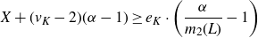 \[ X + (v_K-2)(\alpha-1) \geq e_K \cdot \left( \frac{\alpha}{m_2(L)}-1 \right) \]
for every $L \in \mathcal{L}$
and every non-empty
$L \in \mathcal{L}$
and every non-empty $K \subseteq L$
. Moreover, the inequality is strict unless
$K \subseteq L$
. Moreover, the inequality is strict unless $K=K_2$
.
$K=K_2$
.
Proof. Without loss of generality, we may assume that $m_2(L) \lt \alpha$
and that
$m_2(L) \lt \alpha$
and that $v_K \gt 2$
, as otherwise the statement holds vacuously (recall from Lemma 3·4 that
$v_K \gt 2$
, as otherwise the statement holds vacuously (recall from Lemma 3·4 that $\alpha = m_2(\mathcal{H},\mathcal{L}) \gt m_2(\mathcal{L}) \gt 1$
). Fix some
$\alpha = m_2(\mathcal{H},\mathcal{L}) \gt m_2(\mathcal{L}) \gt 1$
). Fix some $L \in \mathcal{L}$
and a nonempty
$L \in \mathcal{L}$
and a nonempty $K \subseteq L$
. Recall that each
$K \subseteq L$
. Recall that each $H \in \mathcal{H}$
is strictly
$H \in \mathcal{H}$
is strictly $m_2(\cdot,\mathcal{L})$
-balanced and satisfies
$m_2(\cdot,\mathcal{L})$
-balanced and satisfies $m_2(H,\mathcal{L}) \geq m_2(\mathcal{H},\mathcal{L})=\alpha$
. This implies that
$m_2(H,\mathcal{L}) \geq m_2(\mathcal{H},\mathcal{L})=\alpha$
. This implies that
 \[ \frac{e_H}{v_H-2+1/m_2(\mathcal{L})} \geq \alpha \]
or, equivalently,
 \[ e_H \geq \alpha \cdot (v_H-2) + \frac{\alpha}{m_2(\mathcal{L})}. \]
Consequently,
 \[ X = \min_{H \in \mathcal{H}} \{(e_H -1) - \alpha \cdot (v_H-2) \} \geq \frac{\alpha}{m_2(\mathcal{L})}-1 \geq \frac{\alpha}{m_2(L)}-1, \]
where the final inequality uses that $m_2(L)\geq m_2(\mathcal{L})$
.
$m_2(L)\geq m_2(\mathcal{L})$
.
Since L is strictly 2-balanced and we assumed that $m_2(L) \lt \alpha$
, we have
$m_2(L) \lt \alpha$
, we have
 \[ (e_K-1) \cdot \left( \frac{\alpha}{m_2(L)}-1 \right) \leq m_2(L) \cdot (v_K-2) \cdot \left( \frac{\alpha}{m_2(L)}-1 \right) = (v_K-2) (\alpha-m_2(L)). \]
Rearranging the above inequality, we obtain
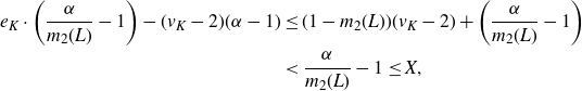 \begin{align*} e_K \cdot \left( \frac{\alpha}{m_2(L)}-1 \right) - (v_K-2)(\alpha-1) &\leq (1-m_2(L))(v_K-2) + \left( \frac{\alpha}{m_2(L)}-1 \right)\\ &\lt \frac{\alpha}{m_2(L)}-1 \leq X, \end{align*}
where the penultimate inequality uses the assumption that $v_K \gt 2$
.
$v_K \gt 2$
.
4. Proof of the probabilistic lemma
In this section, we prove Theorem 1·10. We in fact prove the following more precise statement.
Lemma 4·1 (Theorem 1·10, rephrased). Let $(\mathcal{H},\mathcal{L})$
be a strictly balanced pair of finite families of graphs satisfying
$(\mathcal{H},\mathcal{L})$
be a strictly balanced pair of finite families of graphs satisfying $m_2(\mathcal{H})>m_2(\mathcal{L})$
. There exists a constant
$m_2(\mathcal{H})>m_2(\mathcal{L})$
. There exists a constant $c>0$
such that the following holds. If
$c>0$
such that the following holds. If $p \leq cn^{-1/m_2(\mathcal{H},\mathcal{L})}$
, then a.a.s. every
$p \leq cn^{-1/m_2(\mathcal{H},\mathcal{L})}$
, then a.a.s. every $G \subseteq G_{n,p}$
which supports a core satisfies
$G \subseteq G_{n,p}$
which supports a core satisfies $m(G) \leq m_2(\mathcal{H},\mathcal{L})$
.
$m(G) \leq m_2(\mathcal{H},\mathcal{L})$
.
Note that this immediately implies the difficult direction in Theorem 1·10. Indeed, given a tuple $(\mathcal{H}_1, \dotsc, \mathcal{H}_r)$
, we first define a family
$(\mathcal{H}_1, \dotsc, \mathcal{H}_r)$
, we first define a family $\mathcal{L}$
by replacing each graph in
$\mathcal{L}$
by replacing each graph in $\mathcal{H}_2$
with a strictly 2-balanced subgraph of maximal 2-density. We then likewise define
$\mathcal{H}_2$
with a strictly 2-balanced subgraph of maximal 2-density. We then likewise define $\mathcal{H}$
by replacing every graph in
$\mathcal{H}$
by replacing every graph in $\mathcal{H}_1$
with a strictly balanced subgraph with respect to
$\mathcal{H}_1$
with a strictly balanced subgraph with respect to $m_2(\cdot, \mathcal{L})$
which achieves the maximum. Note that
$m_2(\cdot, \mathcal{L})$
which achieves the maximum. Note that $(\mathcal{H},\mathcal{L})$
is a strictly balanced pair and that
$(\mathcal{H},\mathcal{L})$
is a strictly balanced pair and that $m_2(\mathcal{H}, \mathcal{L}) = m_2(\mathcal{H}_1,\mathcal{H}_2)$
.
$m_2(\mathcal{H}, \mathcal{L}) = m_2(\mathcal{H}_1,\mathcal{H}_2)$
.
Now, any graph that is Ramsey for $(\mathcal{H}_1, \dotsc, \mathcal{H}_r)$
must also be Ramsey for
$(\mathcal{H}_1, \dotsc, \mathcal{H}_r)$
must also be Ramsey for $(\mathcal{H}, \mathcal{L})$
, and must therefore contain a minimal
$(\mathcal{H}, \mathcal{L})$
, and must therefore contain a minimal $(\mathcal{H},\mathcal{L})$
-Ramsey graph
$(\mathcal{H},\mathcal{L})$
-Ramsey graph $G$
. The graph
$G$
. The graph $G$
will then have two properties. First, by Lemma 3·2 it supports an
$G$
will then have two properties. First, by Lemma 3·2 it supports an $(\mathcal{H}, \mathcal{L})$
-core. Second, by the deterministic lemma (i.e., the assumption of Theorem 1·10) we have that
$(\mathcal{H}, \mathcal{L})$
-core. Second, by the deterministic lemma (i.e., the assumption of Theorem 1·10) we have that $m(G) \gt m_2(\mathcal{H}, \mathcal{L})$
. However, Lemma 4·1 asserts that when
$m(G) \gt m_2(\mathcal{H}, \mathcal{L})$
. However, Lemma 4·1 asserts that when $p \le cn^{-1/m_2(\mathcal{H}_1,\mathcal{H}_2)}$
then a.a.s.
$p \le cn^{-1/m_2(\mathcal{H}_1,\mathcal{H}_2)}$
then a.a.s. $G_{n,p}$
does not contain subgraphs G with both these properties, implying that a.a.s.
$G_{n,p}$
does not contain subgraphs G with both these properties, implying that a.a.s. $G_{n,p}$
is not Ramsey for the tuple
$G_{n,p}$
is not Ramsey for the tuple $(\mathcal{H}_1, \dotsc, \mathcal{H}_r)$
.
$(\mathcal{H}_1, \dotsc, \mathcal{H}_r)$
.
Our proof of Lemma 4·1 follows closely the proof of the probabilistic lemma in recent work of the first two authors [
Reference Kuperwasser and Samotij17
]. Fix a strictly balanced pair $(\mathcal{H},\mathcal{L})$
of families satisfying
$(\mathcal{H},\mathcal{L})$
of families satisfying $m_2(\mathcal{H})>m_2(\mathcal{L})$
, and let
$m_2(\mathcal{H})>m_2(\mathcal{L})$
, and let $\alpha \;:\!=\; m_2(\mathcal{H},\mathcal{L})$
. Let
$\alpha \;:\!=\; m_2(\mathcal{H},\mathcal{L})$
. Let $\mathcal{G}_{\mathrm{bad}}$
denote the set of graphs
$\mathcal{G}_{\mathrm{bad}}$
denote the set of graphs $G \subseteq K_n$
which support a core and satisfy
$G \subseteq K_n$
which support a core and satisfy $m(G) \gt m_2(\mathcal{H},\mathcal{L})$
. The key lemma, which implies Lemma 4·1, is as follows.
$m(G) \gt m_2(\mathcal{H},\mathcal{L})$
. The key lemma, which implies Lemma 4·1, is as follows.
Lemma 4·2. There exist constants $\Lambda,K>0$
and a collection
$\Lambda,K>0$
and a collection $\mathcal{S}$
of subgraphs of
$\mathcal{S}$
of subgraphs of $K_n$
satisfying the following properties:
$K_n$
satisfying the following properties:
-
(a) every element of
$\mathcal{G}_{\mathrm{bad}}$
contains some
$S \in \mathcal{S}$
as a subgraph; -
(b) every
$S \in \mathcal{S}$
satisfies at least one of the following three conditions:-
(i)
$v_S \geq \log n$
and
$e_S \geq \alpha \cdot (v_S-2)$
; -
(ii)
$v_S \lt \log n$
and
$e_S \geq \alpha \cdot v_S + 1$
; -
(iii)
$v_S \leq K$
and
$m(S) \gt \alpha$
.
-
-
(c) for every
$k \in [\![{n}]\!]$
, there are at most
$(\Lambda n)^k$
graphs
$S \in \mathcal{S}$
with
$v_S = k$
.


Before we prove Lemma 4·2, let us see why it implies Lemma 4·1.
Proof of Lemma 4·1. Recall that $p \leq cn^{-1/\alpha}$
, for a small constant
$p \leq cn^{-1/\alpha}$
, for a small constant $c=c(\mathcal{H},\mathcal{L})$
to be chosen later. We wish to prove that a.a.s.
$c=c(\mathcal{H},\mathcal{L})$
to be chosen later. We wish to prove that a.a.s. $G_{n,p}$
contains no element of
$G_{n,p}$
contains no element of $\mathcal{G}_{\mathrm{bad}}$
. By Lemma 4·2(a), it suffices to prove that a.a.s.
$\mathcal{G}_{\mathrm{bad}}$
. By Lemma 4·2(a), it suffices to prove that a.a.s. $G_{n,p}$
contains no element of
$G_{n,p}$
contains no element of $\mathcal{S}$
. By (b), the elements of
$\mathcal{S}$
. By (b), the elements of $\mathcal{S}$
are of three types, each of which we deal with separately. First, recall that for any fixed graph
$\mathcal{S}$
are of three types, each of which we deal with separately. First, recall that for any fixed graph $S$
with
$S$
with $m(S) \gt \alpha$
, we have that
$m(S) \gt \alpha$
, we have that $\mathrm{Pr}(S \subseteq G_{n,p})=o(1)$
(see e.g. [
Reference Janson, Łuczak and Ruciński14
, Theorem 3·4]). As there are only a constant number of graphs on at most K vertices, we may apply the union bound and conclude that a.a.s. no graph
$\mathrm{Pr}(S \subseteq G_{n,p})=o(1)$
(see e.g. [
Reference Janson, Łuczak and Ruciński14
, Theorem 3·4]). As there are only a constant number of graphs on at most K vertices, we may apply the union bound and conclude that a.a.s. no graph $S$
satisfying
$S$
satisfying $v_S \leq K$
and
$v_S \leq K$
and $m(S) \gt \alpha$
appears in
$m(S) \gt \alpha$
appears in $G_{n,p}$
. This deals with the elements of
$G_{n,p}$
. This deals with the elements of $\mathcal{S}$
corresponding to case (iii).
$\mathcal{S}$
corresponding to case (iii).
Let $\mathcal{S}' \subseteq \mathcal{S}$
be the set of
$\mathcal{S}' \subseteq \mathcal{S}$
be the set of $S \in \mathcal{S}$
which lie in cases (i) or (ii). We have that
$S \in \mathcal{S}$
which lie in cases (i) or (ii). We have that
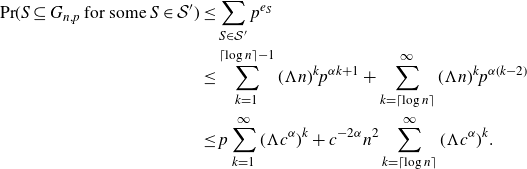 \begin{align*} \mathrm{Pr}(S \subseteq G_{n,p} \text{ for some }S \in \mathcal{S}') &\leq \sum_{S \in \mathcal{S}'} p^{e_S}\\ &\leq \sum_{k=1}^{\lceil \log n \rceil-1} (\Lambda n)^k p^{\alpha k + 1} + \sum_{k=\lceil \log n \rceil}^\infty (\Lambda n)^k p^{\alpha(k-2)}\\ &\leq p\sum_{k=1}^{\infty} (\Lambda c^\alpha)^k + c^{-2\alpha}n^2 \sum_{k=\lceil \log n \rceil}^\infty (\Lambda c^\alpha)^k. \end{align*}
We now choose c so that $\Lambda c^\alpha =e^{-3}$
. Then the first sum above can be bounded by p, which tends to 0 as
$\Lambda c^\alpha =e^{-3}$
. Then the first sum above can be bounded by p, which tends to 0 as $n \to \infty$
. The second term can be bounded by
$n \to \infty$
. The second term can be bounded by $2c^{-2\alpha} n^{-1}$
, which also tends to 0 as
$2c^{-2\alpha} n^{-1}$
, which also tends to 0 as $n \to \infty$
. All in all, we find that a.a.s.
$n \to \infty$
. All in all, we find that a.a.s. $G_{n,p}$
does not contain any graph in
$G_{n,p}$
does not contain any graph in $\mathcal{S}$
, as claimed.
$\mathcal{S}$
, as claimed.
4·1. The exploration process and the proof of Lemma 4·2
In this section, we prove Lemma 4·2. We will construct the family $\mathcal{S}$
by considering an exploration process on the set
$\mathcal{S}$
by considering an exploration process on the set $\mathcal{G}$
of graphs
$\mathcal{G}$
of graphs $G \subseteq K_n$
which support a core. For each such
$G \subseteq K_n$
which support a core. For each such $G \in \mathcal{G}$
, let us arbitrarily choose collections
$G \in \mathcal{G}$
, let us arbitrarily choose collections $\mathcal{F}_\mathcal{H} \subseteq \mathcal{F}_\mathcal{H}[G]$
and
$\mathcal{F}_\mathcal{H} \subseteq \mathcal{F}_\mathcal{H}[G]$
and $\mathcal{F}_\mathcal{L} \subseteq \mathcal{F}_\mathcal{L}[G]$
such that
$\mathcal{F}_\mathcal{L} \subseteq \mathcal{F}_\mathcal{L}[G]$
such that $(G,\mathcal{F}_\mathcal{H},\mathcal{F}_\mathcal{L})$
is a core. From now on, by copies of graphs from
$(G,\mathcal{F}_\mathcal{H},\mathcal{F}_\mathcal{L})$
is a core. From now on, by copies of graphs from $\mathcal{H},\mathcal{L}$
in G, we mean only those copies that belong to the families
$\mathcal{H},\mathcal{L}$
in G, we mean only those copies that belong to the families $\mathcal{F}_\mathcal{H}, \mathcal{F}_\mathcal{L}$
, respectively. This subtlety will be extremely important in parts of the analysis.
$\mathcal{F}_\mathcal{H}, \mathcal{F}_\mathcal{L}$
, respectively. This subtlety will be extremely important in parts of the analysis.
We first fix arbitrary orderings on the graphs in $\mathcal{H}$
and
$\mathcal{H}$
and $\mathcal{L}$
. Additionally, we fix a labeling of the vertices of
$\mathcal{L}$
. Additionally, we fix a labeling of the vertices of $K_n$
, which induces an ordering of all subgraphs according to the lexicographic order. Together with the ordering on
$K_n$
, which induces an ordering of all subgraphs according to the lexicographic order. Together with the ordering on $\mathcal{H},\mathcal{L}$
, we obtain a lexicographic ordering on all copies in
$\mathcal{H},\mathcal{L}$
, we obtain a lexicographic ordering on all copies in $K_n$
of graphs in
$K_n$
of graphs in $\mathcal{H},\mathcal{L}$
. Now, given a
$\mathcal{H},\mathcal{L}$
. Now, given a $G \in \mathcal{G}$
, we build a sequence
$G \in \mathcal{G}$
, we build a sequence $G_0 \subsetneq G_1 \subsetneq \dotsb \subseteq G$
of graphs with no isolated edges as follows. We start with
$G_0 \subsetneq G_1 \subsetneq \dotsb \subseteq G$
of graphs with no isolated edges as follows. We start with $G_0$
being the graph comprising only the smallest edge of G and no further vertices. As long as
$G_0$
being the graph comprising only the smallest edge of G and no further vertices. As long as $G_i \neq G$
, do the following: Since
$G_i \neq G$
, do the following: Since $G \neq G_i$
and
$G \neq G_i$
and $(G, \mathcal{F}_\mathcal{H}, \mathcal{F}_\mathcal{L})$
is a core, there must be some copy of a graph from
$(G, \mathcal{F}_\mathcal{H}, \mathcal{F}_\mathcal{L})$
is a core, there must be some copy of a graph from $\mathcal{H} \cup \mathcal{L}$
which belongs to
$\mathcal{H} \cup \mathcal{L}$
which belongs to $\mathcal{F}_\mathcal{H} \cup \mathcal{F}_\mathcal{L}$
that intersects
$\mathcal{F}_\mathcal{H} \cup \mathcal{F}_\mathcal{L}$
that intersects $G_i$
in at least one edge but is not fully contained in
$G_i$
in at least one edge but is not fully contained in $G_i$
. Call such an overlapping copy regular if it intersects
$G_i$
. Call such an overlapping copy regular if it intersects $G_i$
in exactly one edge (and thus exactly two vertices), called its root; otherwise, call the copy degenerate. We form
$G_i$
in exactly one edge (and thus exactly two vertices), called its root; otherwise, call the copy degenerate. We form $G_{i+1}$
from
$G_{i+1}$
from $G_i$
as follows:
$G_i$
as follows:
-
(1) Suppose first that there is an overlapping copy of some graph in
$\mathcal{H}$
(be it regular or degenerate). We form
$G_{i+1}$
by adding to
$G_i$
the smallest (according to the lexicographic order) such copy. We call
$G_i \to G_{i+1}$
a degenerate
$\mathcal{H}$
-step. -
(2) Otherwise, there must be an overlapping copy
$\widehat{L}$
of some
$L\in \mathcal{L}$
. Note that, for every edge
$e \in \widehat{L} \setminus G_i$
, there must be a copy of some
$H \in \mathcal{H}$
that meets
$\widehat{L}$
only at e, as
$(G, \mathcal{F}_\mathcal{H}, \mathcal{F}_\mathcal{L})$
is a core. Note further that this copy of H does not intersect
$G_i$
, as otherwise we would perform a degenerate
$\mathcal{H}$
-step. We pick the smallest such copy for every
$e \in \widehat{L} \setminus G_i$
, and call it
$\widehat{H_e}$
(note that the graphs
$H_e \in \mathcal{H}$
such that
$H_e \cong \widehat{H_e}$
may be different for different choices of e). We say that
$\widehat{L}$
is pristine if it is regular and the graphs
$\{\widehat{H_e}\}_{e \in \widehat{L} \setminus G_i}$
are all vertex-disjoint (apart from the intersections that they are forced to have in
$V(\widehat{L})$
).


-
(2·1) If there is a pristine copy of some graph in
$\mathcal{L}$
, we pick the smallest one in the following sense: First, among all edges of
$G_i$
that are roots of a pristine copy of some graph in
$\mathcal{L}$
, we choose the one that arrived to
$G_i$
earliest. Second, among all pristine copies that are rooted at this edge, we pick the smallest (according to the lexicographic order). We then form
$G_{i+1}$
by adding to
$G_i$
this smallest copy
$\widehat{L}$
as well as all
$\widehat{H_e}$
where
$e \in \widehat{L} \setminus G_i$
. We call
$G_i \to G_{i+1}$
a pristine step. -
(2·2) If there are no pristine copies of any graph in
$\mathcal{L}$
, we pick the smallest (according to the lexicographic order) overlapping copy
$\widehat{L}$
of a graph in
$\mathcal{L}$
and we still form
$G_{i+1}$
by adding to
$G_i$
the union of
$\widehat{L}$
and all its
$\widehat{H_e}$
with
$e \in \widehat{L} \setminus G_i$
. We call
$G_i \to G_{i+1}$
a degenerate
$\mathcal{L}$
-step.


We define the balance of $G_i$
to be
$G_i$
to be
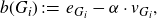 \[ b(G_i) \;:\!=\; e_{G_i} - \alpha \cdot v_{G_i},\]
where we recall that $\alpha = m_2(\mathcal{H},\mathcal{L})$
. The key result we will need in order to prove (b) is the following lemma. We remark that a similar result was proved by Hyde [
Reference Hyde13
, Claims 6·2 and 6·3]; it plays an integral role in his approach to the Kohayakawa–Kreuter conjecture.
$\alpha = m_2(\mathcal{H},\mathcal{L})$
. The key result we will need in order to prove (b) is the following lemma. We remark that a similar result was proved by Hyde [
Reference Hyde13
, Claims 6·2 and 6·3]; it plays an integral role in his approach to the Kohayakawa–Kreuter conjecture.
Lemma 4·3. For every i, we have that $b(G_{i+1}) \geq b(G_i)$
. Moreover, there exists some
$b(G_{i+1}) \geq b(G_i)$
. Moreover, there exists some $\delta=\delta(\mathcal{H},\mathcal{L})>0$
such that
$\delta=\delta(\mathcal{H},\mathcal{L})>0$
such that $b(G_{i+1}) \geq b(G_i)+\delta$
if
$b(G_{i+1}) \geq b(G_i)+\delta$
if $G_{i+1}$
was obtained from
$G_{i+1}$
was obtained from $G_i$
by a degenerate step.
$G_i$
by a degenerate step.
As the proof of Lemma 4·3 is somewhat technical, we defer it to Section 4.2. For the moment, we assume the result and continue the discussion of how we construct the family $\mathcal{S}$
. We now let
$\mathcal{S}$
. We now let $\Gamma \;:\!=\; \lceil 2\alpha/\delta \rceil$
, where
$\Gamma \;:\!=\; \lceil 2\alpha/\delta \rceil$
, where $\delta$
is the constant from Lemma 4·3. For
$\delta$
is the constant from Lemma 4·3. For $G \in \mathcal{G}$
, let
$G \in \mathcal{G}$
, let
 \[ \tau(G) \;:\!=\; \min\{i \;:\; v_{G_i} \geq \log n \text{ or } G_i = G \text{ or }G_{i-1} \to G_i\text{ is the $\Gamma$th degenerate step}\}\]
and let
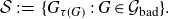 \begin{equation} \mathcal{S} \;:\!=\; \{G_{\tau(G)} \;:\; G \in \mathcal{G}_{\mathrm{bad}}\}.\end{equation}
Having defined the family $\mathcal{S}$
, we are ready to prove Lemma 4·2. Since the definition of
$\mathcal{S}$
, we are ready to prove Lemma 4·2. Since the definition of $\mathcal{S}$
clearly guarantees property (a), it remains to establish properties (b) and (c). We begin by showing that, if K is sufficiently large (depending only on
$\mathcal{S}$
clearly guarantees property (a), it remains to establish properties (b) and (c). We begin by showing that, if K is sufficiently large (depending only on $\mathcal{H}$
and
$\mathcal{H}$
and $\mathcal{L}$
), then (b) holds.
$\mathcal{L}$
), then (b) holds.
Proof of Lemma 4·2(b). Let $\delta$
be the constant from Lemma 4·3, let
$\delta$
be the constant from Lemma 4·3, let $M \;:\!=\; \max \{e_L \cdot v_H\;:\; H \in \mathcal{H}, L \in \mathcal{L}\}$
, and let
$M \;:\!=\; \max \{e_L \cdot v_H\;:\; H \in \mathcal{H}, L \in \mathcal{L}\}$
, and let $K \;:\!=\; 2M^2 \Gamma$
; note that each of these parameters depends only on
$K \;:\!=\; 2M^2 \Gamma$
; note that each of these parameters depends only on $\mathcal{H}$
and
$\mathcal{H}$
and $\mathcal{L}$
.
$\mathcal{L}$
.
Every $S \in \mathcal{S}$
is of the form
$S \in \mathcal{S}$
is of the form $G_{\tau(G)}$
for some
$G_{\tau(G)}$
for some $G \in \mathcal{G}_{\mathrm{bad}}$
. We split into cases depending on which of the three conditions defining
$G \in \mathcal{G}_{\mathrm{bad}}$
. We split into cases depending on which of the three conditions defining $\tau(G)$
caused us to stop the exploration. Suppose first that we stopped the exploration because
$\tau(G)$
caused us to stop the exploration. Suppose first that we stopped the exploration because $v_S \geq \log n$
. By Lemma 4·3, we have that
$v_S \geq \log n$
. By Lemma 4·3, we have that
 \[ e_S - \alpha \cdot v_S= b(S) = b(G_{\tau(G)}) \geq b(G_0) = 1-2\alpha, \]
and therefore $e_S \geq \alpha \cdot (v_S-2)$
. This yields case 4.2.
$e_S \geq \alpha \cdot (v_S-2)$
. This yields case 4.2.
Next, suppose we stopped the exploration because step $G_{\tau(G)-1} \to G_{\tau(G)}$
was the
$G_{\tau(G)-1} \to G_{\tau(G)}$
was the $\Gamma$
th degenerate step. As we are not in the previous case, we may assume that
$\Gamma$
th degenerate step. As we are not in the previous case, we may assume that $v_S <\log n$
. By Lemma 4·3 and our choice of
$v_S <\log n$
. By Lemma 4·3 and our choice of $\Gamma$
, we have that
$\Gamma$
, we have that
 \[ e_S - \alpha \cdot v_S =b(S) = b(G_{\tau(G)}) \geq b(G_0) + \Gamma \delta \geq 1-2\alpha + 2\alpha = 1. \]
Rearranging, we see that $e_S \geq \alpha \cdot v_S + 1$
, yielding case (ii).
$e_S \geq \alpha \cdot v_S + 1$
, yielding case (ii).
The remaining case is when we stop because $S = G \in \mathcal{G}_{\mathrm{bad}}$
. Since the definition of
$S = G \in \mathcal{G}_{\mathrm{bad}}$
. Since the definition of $\mathcal{G}_{\mathrm{bad}}$
implies that
$\mathcal{G}_{\mathrm{bad}}$
implies that $m(G) \gt \alpha$
, in order to establish (iii), we only need to show that
$m(G) \gt \alpha$
, in order to establish (iii), we only need to show that $v_G \leq K$
. For this proof, we need to keep track of another parameter during the exploration process, which we term the pristine boundary. Recall that at every pristine step, we add to
$v_G \leq K$
. For this proof, we need to keep track of another parameter during the exploration process, which we term the pristine boundary. Recall that at every pristine step, we add to $G_i$
a copy
$G_i$
a copy $\widehat{L}$
of some
$\widehat{L}$
of some $L \in \mathcal{L}$
that intersects
$L \in \mathcal{L}$
that intersects $G_i$
in a single edge (the root), and then add copies
$G_i$
in a single edge (the root), and then add copies $\widehat{H_e}$
of graphs
$\widehat{H_e}$
of graphs $H_e \in \mathcal{H}$
, one for every edge of
$H_e \in \mathcal{H}$
, one for every edge of $\widehat{L}$
apart from the root. Let us say that the boundary of this step is the set of all newly added vertices that are not in
$\widehat{L}$
apart from the root. Let us say that the boundary of this step is the set of all newly added vertices that are not in $\widehat{L}$
, that is, the set
$\widehat{L}$
, that is, the set $V(G_{i+1}) \setminus (V(G_i) \cup V(\widehat{L})) = (\bigcup_{e \in \widehat{L} \setminus G_i} V(\widehat{H_e})) \setminus V(\widehat{L})$
. Note that the size of the boundary is equal to
$V(G_{i+1}) \setminus (V(G_i) \cup V(\widehat{L})) = (\bigcup_{e \in \widehat{L} \setminus G_i} V(\widehat{H_e})) \setminus V(\widehat{L})$
. Note that the size of the boundary is equal to
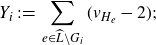 \[ Y_i \;:\!=\; \sum_{e \in \widehat{L} \setminus G_i} (v_{H_e}-2); \]
indeed, by the definition of pristine steps, the copies $\widehat{H_e}$
are vertex-disjoint outside of
$\widehat{H_e}$
are vertex-disjoint outside of $V(\widehat{L})$
.
$V(\widehat{L})$
.
We claim that $Y_i \geq 3$
. To see this, note first that L has at least three edges, as it is not a forest. Similarly, each
$Y_i \geq 3$
. To see this, note first that L has at least three edges, as it is not a forest. Similarly, each $H_e$
has at least three vertices. Putting these together, we see that there are at least two terms in the sum, and every term in the sum is at least one. Thus,
$H_e$
has at least three vertices. Putting these together, we see that there are at least two terms in the sum, and every term in the sum is at least one. Thus, $Y_i \geq 3$
unless
$Y_i \geq 3$
unless $e_L=3$
and
$e_L=3$
and $v_{H_e}=3$
for all e. But in this case,
$v_{H_e}=3$
for all e. But in this case, $L = K_3 = H_e \in \mathcal{H}$
for all e, which means that
$L = K_3 = H_e \in \mathcal{H}$
for all e, which means that $\widehat{L}$
should have been added to
$\widehat{L}$
should have been added to $G_i$
as a degenerate
$G_i$
as a degenerate $\mathcal{H}$
-step.
$\mathcal{H}$
-step.
We now inductively define the pristine boundary $\partial G_i$
of
$\partial G_i$
of $G_i$
as follows. We set
$G_i$
as follows. We set $\partial G_0\;:\!=\; \varnothing$
. If
$\partial G_0\;:\!=\; \varnothing$
. If $G_i \to G_{i+1}$
is a pristine step, then we delete from
$G_i \to G_{i+1}$
is a pristine step, then we delete from $\partial G_i$
the two endpoints of the root and add to
$\partial G_i$
the two endpoints of the root and add to $\partial G_i$
the boundary of this pristine step. Note that
$\partial G_i$
the boundary of this pristine step. Note that $\lvert\partial G_{i+1}\rvert \geq \lvert\partial G_i\rvert + Y_i - 2 \geq \lvert\partial G_i\rvert + 1$
. On the other hand, if
$\lvert\partial G_{i+1}\rvert \geq \lvert\partial G_i\rvert + Y_i - 2 \geq \lvert\partial G_i\rvert + 1$
. On the other hand, if $G_i \to G_{i+1}$
is a degenerate step, then we only remove vertices from
$G_i \to G_{i+1}$
is a degenerate step, then we only remove vertices from $\partial G_i$
, without adding any new vertices. Namely, we remove from
$\partial G_i$
, without adding any new vertices. Namely, we remove from $\partial G_i$
all the vertices which are included in the newly added graphs. In other words, if we performed a degenerate
$\partial G_i$
all the vertices which are included in the newly added graphs. In other words, if we performed a degenerate $\mathcal{H}$
-step by adding a copy
$\mathcal{H}$
-step by adding a copy $\widehat{H}$
of some graph in
$\widehat{H}$
of some graph in $\mathcal{H}$
, we set
$\mathcal{H}$
, we set $\partial G_{i+1} \;:\!=\; \partial G_i \setminus V(\widehat{H})$
. Similarly, if we performed a degenerate
$\partial G_{i+1} \;:\!=\; \partial G_i \setminus V(\widehat{H})$
. Similarly, if we performed a degenerate $\mathcal{L}$
-step by adding a copy
$\mathcal{L}$
-step by adding a copy $\widehat{L}$
of some graph in
$\widehat{L}$
of some graph in $\mathcal{L}$
along with the graphs
$\mathcal{L}$
along with the graphs $\widehat{H_e}$
for all
$\widehat{H_e}$
for all $e \in \widehat{L} \setminus G_i$
, we set
$e \in \widehat{L} \setminus G_i$
, we set $\partial G_{i+1} \;:\!=\; \partial G_i \setminus (V(\widehat{L}) \cup \bigcup_e V(\widehat{H_e}))$
. Note that in either case
$\partial G_{i+1} \;:\!=\; \partial G_i \setminus (V(\widehat{L}) \cup \bigcup_e V(\widehat{H_e}))$
. Note that in either case $\lvert\partial G_{i+1}\rvert \geq \lvert\partial G_i\rvert - M$
, as the union of all graphs added in each degenerate step can have at most M vertices.
$\lvert\partial G_{i+1}\rvert \geq \lvert\partial G_i\rvert - M$
, as the union of all graphs added in each degenerate step can have at most M vertices.
We now argue that $\partial G_{\tau(G)}=\varnothing$
. Indeed, suppose we had some vertex
$\partial G_{\tau(G)}=\varnothing$
. Indeed, suppose we had some vertex $v \in \partial G_{\tau(G)}$
. By definition, v was added during a pristine step, as a vertex of a copy
$v \in \partial G_{\tau(G)}$
. By definition, v was added during a pristine step, as a vertex of a copy $\widehat{H_e}$
of some graph
$\widehat{H_e}$
of some graph $H_e \in \mathcal{H}$
, and was never touched again. Observe that v is incident to some edge uv of
$H_e \in \mathcal{H}$
, and was never touched again. Observe that v is incident to some edge uv of $\widehat{H_e}$
that was not touched by any later step of the exploration. However, as
$\widehat{H_e}$
that was not touched by any later step of the exploration. However, as $(G, \mathcal{F}_\mathcal{H}, \mathcal{F}_\mathcal{L})$
is a core and
$(G, \mathcal{F}_\mathcal{H}, \mathcal{F}_\mathcal{L})$
is a core and $\widehat{H_e} \in \mathcal{F}_\mathcal{H}$
, there must be some
$\widehat{H_e} \in \mathcal{F}_\mathcal{H}$
, there must be some $\widehat{L_{uv}} \in \mathcal{F}_\mathcal{L}$
that intersects
$\widehat{L_{uv}} \in \mathcal{F}_\mathcal{L}$
that intersects $\widehat{H_e}$
only at uv. Moreover, as
$\widehat{H_e}$
only at uv. Moreover, as $\widehat{L_{uv}}$
has minimum degree at least two (by the strict 2-balancedness assumption), there is some edge
$\widehat{L_{uv}}$
has minimum degree at least two (by the strict 2-balancedness assumption), there is some edge $vw \in \widehat{L_{uv}} \setminus uv$
that is incident to v. Since we assumed that
$vw \in \widehat{L_{uv}} \setminus uv$
that is incident to v. Since we assumed that $G_{\tau(G)} = G$
, the edge vw must have been added at some point, a contradiction to the assumption that v was never touched again.
$G_{\tau(G)} = G$
, the edge vw must have been added at some point, a contradiction to the assumption that v was never touched again.
Finally, since $\lvert\partial G_i\rvert$
increases by at least one during every pristine step and decreases by at most M during each of the at most
$\lvert\partial G_i\rvert$
increases by at least one during every pristine step and decreases by at most M during each of the at most $\Gamma$
degenerate steps, in order to achieve
$\Gamma$
degenerate steps, in order to achieve $\partial G_{\tau(G)}=\varnothing$
, there can be at most
$\partial G_{\tau(G)}=\varnothing$
, there can be at most $M\Gamma$
pristine steps. In particular, the total number of exploration steps is at most
$M\Gamma$
pristine steps. In particular, the total number of exploration steps is at most $M\Gamma + \Gamma$
. As each exploration step adds at most M vertices to
$M\Gamma + \Gamma$
. As each exploration step adds at most M vertices to $G_i$
, we conclude that
$G_i$
, we conclude that $v_G \leq M(M\Gamma + \Gamma)+2 \leq K$
. This completes the proof of (iii).
$v_G \leq M(M\Gamma + \Gamma)+2 \leq K$
. This completes the proof of (iii).
Proof of Lemma 4·2(c). Suppose S has k vertices and let $G \in \mathcal{G}_{\mathrm{bad}}$
be such that
$G \in \mathcal{G}_{\mathrm{bad}}$
be such that $S = G_{\tau(G)}$
. We consider the exploration process on G. Note that in every step we add an overlapping copy of a graph from a finite family
$S = G_{\tau(G)}$
. We consider the exploration process on G. Note that in every step we add an overlapping copy of a graph from a finite family $\mathcal{F}$
that comprises all graphs in
$\mathcal{F}$
that comprises all graphs in $\mathcal{H}$
(for the cases where we made a degenerate
$\mathcal{H}$
(for the cases where we made a degenerate $\mathcal{H}$
-step) and graphs in
$\mathcal{H}$
-step) and graphs in $\mathcal{L}$
that have graphs from
$\mathcal{L}$
that have graphs from $\mathcal{H}$
glued on subsets of their edges, with all intersection patterns (for the pristine and degenerate
$\mathcal{H}$
glued on subsets of their edges, with all intersection patterns (for the pristine and degenerate $\mathcal{L}$
-steps). Let
$\mathcal{L}$
-steps). Let $\mathcal{F}^\times$
denote the graphs in
$\mathcal{F}^\times$
denote the graphs in $\mathcal{F}$
that correspond to a pristine step.
$\mathcal{F}$
that correspond to a pristine step.
Now, every degenerate step can be described by specifying the graph $F \in \mathcal{F}$
whose copy
$F \in \mathcal{F}$
whose copy $\widehat{F}$
we are adding, the subgraph
$\widehat{F}$
we are adding, the subgraph $F' \subseteq F$
and the embedding
$F' \subseteq F$
and the embedding $\varphi \colon V(F') \to V(G_i)$
that describe the intersection
$\varphi \colon V(F') \to V(G_i)$
that describe the intersection $\widehat{F} \cap G_i$
, and the sequence of
$\widehat{F} \cap G_i$
, and the sequence of $v_F - v_{F'}$
vertices of
$v_F - v_{F'}$
vertices of $K_n$
that complete
$K_n$
that complete $\varphi$
to an embedding of F into
$\varphi$
to an embedding of F into $K_n$
. Every pristine step is uniquely described by the root edge in
$K_n$
. Every pristine step is uniquely described by the root edge in $G_i$
, the graph
$G_i$
, the graph $F \in \mathcal{F}^\times$
, the edge of F corresponding to the root, and the (ordered sequence of)
$F \in \mathcal{F}^\times$
, the edge of F corresponding to the root, and the (ordered sequence of) $v_F - 2$
vertices of
$v_F - 2$
vertices of $K_n$
that complete the root edge to a copy of F in
$K_n$
that complete the root edge to a copy of F in $K_n$
. There are at most
$K_n$
. There are at most $n^k$
ways to choose the sequence of vertices that were added through this exploration process, in the order that they are introduced to G. Each pristine step adds at least one new vertex, so there are at most k pristine steps. Furthermore, there are always at most
$n^k$
ways to choose the sequence of vertices that were added through this exploration process, in the order that they are introduced to G. Each pristine step adds at least one new vertex, so there are at most k pristine steps. Furthermore, there are always at most $\Gamma$
degenerate steps, meaning that
$\Gamma$
degenerate steps, meaning that $\tau(G) \leq k + \Gamma$
. In particular, there are at most
$\tau(G) \leq k + \Gamma$
. In particular, there are at most $(k + \Gamma) \cdot 2^{k + \Gamma}$
ways to choose
$(k + \Gamma) \cdot 2^{k + \Gamma}$
ways to choose $\tau(G)$
and to specify which steps were pristine.
$\tau(G)$
and to specify which steps were pristine.
For every degenerate step, there are at most
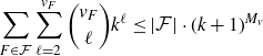 \[\sum_{F \in \mathcal{F}} \sum_{\ell=2}^{v_F} \binom{v_F}{\ell} k^\ell \leq \lvert\mathcal{F}\rvert \cdot (k+1)^{M_v}\]
ways of choosing $F \in \mathcal{F}$
and describing the intersection of its copy
$F \in \mathcal{F}$
and describing the intersection of its copy $\widehat{F}$
with
$\widehat{F}$
with $G_i$
(the set
$G_i$
(the set $V(F') \subseteq V(F)$
and the embedding
$V(F') \subseteq V(F)$
and the embedding $\varphi$
above), where
$\varphi$
above), where $M_v \;:\!=\; \max \{v_F \colon F \in \mathcal{F} \}$
. As for the pristine steps, note that, in the course of our exploration, the sequence of the arrival times of the roots to
$M_v \;:\!=\; \max \{v_F \colon F \in \mathcal{F} \}$
. As for the pristine steps, note that, in the course of our exploration, the sequence of the arrival times of the roots to $G_{\tau(G)}$
must be non-decreasing. This is because as soon as an edge appears in some
$G_{\tau(G)}$
must be non-decreasing. This is because as soon as an edge appears in some $G_i$
, every pristine step that includes it as a root at any later step is already available, and we always choose the one rooted at the edge that arrived to G the earliest. Therefore, there are at most
$G_i$
, every pristine step that includes it as a root at any later step is already available, and we always choose the one rooted at the edge that arrived to G the earliest. Therefore, there are at most $\binom{e_S + k}{k}$
possible sequences of root edges, since this is the number of non-decreasing sequences of length k in
$\binom{e_S + k}{k}$
possible sequences of root edges, since this is the number of non-decreasing sequences of length k in $[\![{e_S}]\!]$
. To supplement this bound, remember that every step increases the number of edges in
$[\![{e_S}]\!]$
. To supplement this bound, remember that every step increases the number of edges in $G_i$
by at most
$G_i$
by at most $M_e \;:\!=\; \max \{e_F \;:\; F \in \mathcal{F} \}$
, which means that
$M_e \;:\!=\; \max \{e_F \;:\; F \in \mathcal{F} \}$
, which means that
 \[e_S \leq 1 + \tau(G)\cdot M_e \leq 1 + (k + \Gamma) \cdot M_e.\]
To summarise, the number of $S \in \mathcal{S}$
with k vertices is at most
$S \in \mathcal{S}$
with k vertices is at most
 \[n^k \cdot (k+ \Gamma) \cdot 2^{k + \Gamma} \cdot \left( \lvert\mathcal{F}\rvert \cdot (k+1)^{M_v}\right)^\Gamma \cdot \binom{(k+\Gamma) \cdot M_e + k + 1}{k} \cdot \left(\lvert\mathcal{F}\rvert \cdot M_e \right)^k.\]
Every term in this product, apart from the first, is bounded by an exponential function of k, since $\Gamma, \lvert\mathcal{F}\rvert, M_v$
, and
$\Gamma, \lvert\mathcal{F}\rvert, M_v$
, and $M_e$
are all constants. Therefore, if we choose
$M_e$
are all constants. Therefore, if we choose $\Lambda = \Lambda(\mathcal{H},\mathcal{L})$
sufficiently large, we find that the number of
$\Lambda = \Lambda(\mathcal{H},\mathcal{L})$
sufficiently large, we find that the number of $S \in \mathcal{S}$
with
$S \in \mathcal{S}$
with $v_S=k$
is at most
$v_S=k$
is at most $(\Lambda n)^k$
, as claimed.
$(\Lambda n)^k$
, as claimed.
4·2. Proof of Lemma 4·3
In this section, we prove Lemma 4·3. The proof is divided into a number of claims. Recall Lemma 3·5, which asserts that
 \[ e_H-e_F \gt m_2(\mathcal{H},\mathcal{L}) \cdot (v_H-v_F) = \alpha \cdot (v_H - v_F)\]
for all $H \in \mathcal{H}$
and all
$H \in \mathcal{H}$
and all $F \subsetneq H$
. This implies that we can choose some
$F \subsetneq H$
. This implies that we can choose some $\delta_1=\delta_1(\mathcal{H},\mathcal{L})>0$
so that
$\delta_1=\delta_1(\mathcal{H},\mathcal{L})>0$
so that
 \begin{equation} e_H-e_F \geq \alpha \cdot(v_H-v_F) + \delta_1\end{equation}
for all $H \in \mathcal{H}$
and all
$H \in \mathcal{H}$
and all $F \subsetneq H$
; we henceforth fix such a
$F \subsetneq H$
; we henceforth fix such a $\delta_1>0$
.
$\delta_1>0$
.
Our first claim deals with the (easy) case that $G_i \to G_{i+1}$
is a degenerate
$G_i \to G_{i+1}$
is a degenerate $\mathcal{H}$
-step.
$\mathcal{H}$
-step.
Claim 4·4 If $G_i \to G_{i+1}$
is a degenerate
$G_i \to G_{i+1}$
is a degenerate $\mathcal{H}$
-step, then
$\mathcal{H}$
-step, then $b(G_{i+1}) \geq b(G_i) + \delta_1$
.
$b(G_{i+1}) \geq b(G_i) + \delta_1$
.
Proof. Suppose we add to $G_i$
a copy of some
$G_i$
a copy of some $H \in \mathcal{H}$
that intersects
$H \in \mathcal{H}$
that intersects $G_i$
on a subgraph
$G_i$
on a subgraph $F \subseteq H$
. This means that
$F \subseteq H$
. This means that
 \[ e_{G_{i+1}} = e_{G_i} + (e_H - e_F) \qquad \text{ and } \qquad v_{G_{i+1}} = v_{G_i} + (v_H - v_F) \]
and thus
 \[ b(G_{i+1}) - b(G_i) = (e_H - e_F) - \alpha\cdot (v_H - v_F) \geq \delta_1, \]
where the inequality follows from (2), as F must be a proper subgraph of H.
Now, suppose that $G_i \to G_{i+1}$
is an
$G_i \to G_{i+1}$
is an $\mathcal{L}$
-step, either degenerate or pristine, which means that we add a copy
$\mathcal{L}$
-step, either degenerate or pristine, which means that we add a copy $\widehat{L}$
of some
$\widehat{L}$
of some $L\in \mathcal{L}$
and then add, for every edge
$L\in \mathcal{L}$
and then add, for every edge $e \in \widehat{L} \setminus G_i$
, a copy
$e \in \widehat{L} \setminus G_i$
, a copy $\widehat{H_e}$
of some
$\widehat{H_e}$
of some $H_e \in \mathcal{H}$
. Let
$H_e \in \mathcal{H}$
. Let $G_i' \;:\!=\; G_i \cup \widehat{L}$
and let
$G_i' \;:\!=\; G_i \cup \widehat{L}$
and let $\widehat{J} \;:\!=\; G_i\cap \widehat{L}$
, so that
$\widehat{J} \;:\!=\; G_i\cap \widehat{L}$
, so that $\widehat{J} \cong J$
for some
$\widehat{J} \cong J$
for some $J \subsetneq L$
with at least one edge. Note that
$J \subsetneq L$
with at least one edge. Note that
 \begin{equation} b(G_i') - b(G_i) = (e_L - e_J) - \alpha \cdot (v_L - v_J),\end{equation}
as we add $e_L -e_J$
edges and
$e_L -e_J$
edges and $v_L - v_J$
vertices to
$v_L - v_J$
vertices to $G_i$
when forming
$G_i$
when forming $G_i'$
.
$G_i'$
.
In order to analyse $b(G_{i+1}) - b(G_i')$
, we now define an auxiliary graph
$b(G_{i+1}) - b(G_i')$
, we now define an auxiliary graph $\mathcal{I}$
as follows. Its vertices are the edges of
$\mathcal{I}$
as follows. Its vertices are the edges of $\widehat{L} \setminus \widehat{J}$
. Recall that, for every such edge e, the graph
$\widehat{L} \setminus \widehat{J}$
. Recall that, for every such edge e, the graph $\widehat{H_e} \cong H_e$
intersects the edges of
$\widehat{H_e} \cong H_e$
intersects the edges of $G_i'$
only in the edge e. A pair e, f of edges of
$G_i'$
only in the edge e. A pair e, f of edges of $\widehat{L} \setminus \widehat{J}$
will be adjacent in
$\widehat{L} \setminus \widehat{J}$
will be adjacent in $\mathcal{I}$
if and only if their corresponding graphs
$\mathcal{I}$
if and only if their corresponding graphs $\widehat{H_e}$
and
$\widehat{H_e}$
and $\widehat{H_f}$
share at least one edge (equivalently, the graphs
$\widehat{H_f}$
share at least one edge (equivalently, the graphs $\widehat{H_e} \setminus e$
and
$\widehat{H_e} \setminus e$
and $\widehat{H_f} \setminus f$
share an edge).
$\widehat{H_f} \setminus f$
share an edge).
Denote the connected components of $\mathcal{I}$
by
$\mathcal{I}$
by $K_1, \dotsc, K_m$
and note that each of them corresponds to a subgraph of
$K_1, \dotsc, K_m$
and note that each of them corresponds to a subgraph of $\widehat{L} \setminus\widehat{J}$
. For each
$\widehat{L} \setminus\widehat{J}$
. For each $j \in [\![{m}]\!]$
, let
$j \in [\![{m}]\!]$
, let
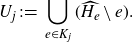 \[ U_j \;:\!=\; \bigcup_{e \in K_j} (\widehat{H_e} \setminus e).\]
Note that the graphs $G_i'$
and
$G_i'$
and $U_1, \dotsc, U_m$
are pairwise edge-disjoint and that each
$U_1, \dotsc, U_m$
are pairwise edge-disjoint and that each $U_j$
shares at least
$U_j$
shares at least $v_{K_j}$
vertices (the endpoints of all the edges of
$v_{K_j}$
vertices (the endpoints of all the edges of $K_j$
) with
$K_j$
) with $G_i'$
. It follows that
$G_i'$
. It follows that
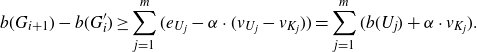 \begin{equation} b(G_{i+1}) - b(G_i') \geq \sum_{j=1}^m (e_{U_j} - \alpha \cdot (v_{U_j} - v_{K_j})) = \sum_{j=1}^m (b(U_j) + \alpha \cdot v_{K_j}).\end{equation}
Finally, as in the statement of Lemma 3·7, define
 \[ X \;:\!=\; \min \{(e_H-1)-\alpha \cdot (v_H-2) \;:\; H \in \mathcal{H}\}.\]
The following claim lies at the heart of the matter.
Claim 4·5. For every $j \in [\![{m}]\!]$
, we have
$j \in [\![{m}]\!]$
, we have
 \[ b(U_j) \geq X - 2\alpha - (v_{K_j}-2) + \min\{\delta_1,1\} \cdot \mathbf{1}_{v_{K_j}>2}. \]
Proof. Since $K_j$
is connected in
$K_j$
is connected in $\mathcal{I}$
, we may order its edges as
$\mathcal{I}$
, we may order its edges as $e_1, \dotsc, e_\ell$
so that, for each
$e_1, \dotsc, e_\ell$
so that, for each $r \in [\![{\ell-1}]\!]$
, the edge
$r \in [\![{\ell-1}]\!]$
, the edge $e_{r+1}$
is
$e_{r+1}$
is $\mathcal{I}$
-adjacent to
$\mathcal{I}$
-adjacent to $\{e_1, \dotsc, e_r\}$
. We define, for each
$\{e_1, \dotsc, e_r\}$
. We define, for each $r \in \{0, \dotsc, \ell\}$
,
$r \in \{0, \dotsc, \ell\}$
,
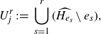 \[ U_j^r \;:\!=\; \bigcup_{s=1}^r (\widehat{H_{e_s}} \setminus e_s), \]
so that $\varnothing = U_j^0 \subseteq \dotsb \subseteq U_j^\ell = U_j$
. Observe that
$\varnothing = U_j^0 \subseteq \dotsb \subseteq U_j^\ell = U_j$
. Observe that
 \[ b(U_j^1) = e_{U_j^1} - \alpha \cdot v_{U_j^1} = (e_{H_{e_1}} -1) - \alpha \cdot v_{H_{e_1}} \geq X - 2\alpha, \]
where the inequality follows from the definition of X.
Suppose now that $r \geq 1$
and let
$r \geq 1$
and let $\widehat{F}$
be the intersection of
$\widehat{F}$
be the intersection of $\widehat{H_{e_{r+1}}} \setminus e_{r+1}$
with
$\widehat{H_{e_{r+1}}} \setminus e_{r+1}$
with $U_j^r$
; note that this intersection is non-empty as
$U_j^r$
; note that this intersection is non-empty as $e_{r+1}$
is
$e_{r+1}$
is $\mathcal{I}$
-adjacent to
$\mathcal{I}$
-adjacent to $\{e_1,\ldots,e_r\}$
. We have
$\{e_1,\ldots,e_r\}$
. We have
 \[ b(U_j^{r+1}) - b(U_j^r) = (e_{H_{e_{r+1}}}-1-e_F) - \alpha \cdot (v_{H_{e_{r+1}}} - v_F). \]
Let $t_{r+1}$
be the number of endpoints of
$t_{r+1}$
be the number of endpoints of $e_{r+1}$
that are not in
$e_{r+1}$
that are not in $U_j^r$
. Suppose first that
$U_j^r$
. Suppose first that $t_{r+1} = 0$
, that is, both endpoints of
$t_{r+1} = 0$
, that is, both endpoints of $e_{r+1}$
are already in
$e_{r+1}$
are already in $U_j^r$
. In this case, both endpoints of
$U_j^r$
. In this case, both endpoints of $e_{r+1}$
also belong to
$e_{r+1}$
also belong to $\widehat{F}$
and thus
$\widehat{F}$
and thus $\widehat{F} \cup e_{r+1}$
is isomorphic to a subgraph
$\widehat{F} \cup e_{r+1}$
is isomorphic to a subgraph $F^+ \subseteq H_{e_{r+1}}$
with
$F^+ \subseteq H_{e_{r+1}}$
with $e_F+1$
edges and
$e_F+1$
edges and $v_F$
vertices, which means that
$v_F$
vertices, which means that
 \[ b(U_j^{r+1}) - b(U_j^r) = (e_{H_{e_{r+1}}} - e_{F^+}) - \alpha \cdot (v_{H_{e_{r+1}}} - v_{F^+}) \geq 0, \]
by Lemma 3·5. In case $t_{r+1} \gt 0$
, F is a proper subgraph of
$t_{r+1} \gt 0$
, F is a proper subgraph of $H_{e_{r+1}}$
and thus we have
$H_{e_{r+1}}$
and thus we have
 \[ b(U_j^{r+1}) - b(U_j^r) \geq \delta_1-1 \geq \delta_1-t_{r+1}, \]
see (2). We may thus conclude that
 \[ b(U_j) = b(U_j^1) + \sum_{r=1}^{\ell-1} (b(U_j^{r+1}) - b(U_j^r)) \geq X - 2\alpha - \sum_{r=1}^{\ell-1} t_{r+1} + \delta_1 \cdot \mathbf{1}_{t_2+\dotsb+t_\ell>0}. \]
The desired inequality follows as $t_2 + \dotsb + t_{\ell} = \lvert V(K_j) \setminus V(U_j^1)\rvert \leq v_{K_j}-2$
and, further,
$t_2 + \dotsb + t_{\ell} = \lvert V(K_j) \setminus V(U_j^1)\rvert \leq v_{K_j}-2$
and, further, $v_{K_j} \gt 2$
implies that the sum
$v_{K_j} \gt 2$
implies that the sum $t_2+\dotsb+t_\ell$
is either positive or at most
$t_2+\dotsb+t_\ell$
is either positive or at most $v_{K_j}-3$
.
$v_{K_j}-3$
.
We are now ready to show that the balance never decreases when we perform an $\mathcal{L}$
-step.
$\mathcal{L}$
-step.
Claim 4·6. If $G_i \to G_{i+1}$
is an
$G_i \to G_{i+1}$
is an $\mathcal{L}$
-step, then
$\mathcal{L}$
-step, then $b(G_{i+1}) \geq b(G_i)$
. Moreover, if this
$b(G_{i+1}) \geq b(G_i)$
. Moreover, if this $\mathcal{L}$
-step is degenerate, then
$\mathcal{L}$
-step is degenerate, then $b(G_{i+1}) \geq b(G_i) + \delta_2$
for some
$b(G_{i+1}) \geq b(G_i) + \delta_2$
for some $\delta_2>0$
that depends only on
$\delta_2>0$
that depends only on $\mathcal{H}$
and
$\mathcal{H}$
and $\mathcal{L}$
.
$\mathcal{L}$
.
Proof. By (3), (4) and Claim 4·6, we have
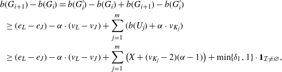 \begin{align*} b&(G_{i+1}) - b(G_i) = b(G_i')-b(G_i) + b(G_{i+1})-b(G_i') \\ &\geq (e_L-e_J) - \alpha \cdot (v_L-v_J) + \sum_{j=1}^m (b(U_j) + \alpha \cdot v_{K_j}) \\ &\geq (e_L-e_J) - \alpha \cdot (v_L-v_J) + \sum_{j=1}^m \left( X + (v_{K_j}-2)(\alpha-1) \right) + \min\{\delta_1,1\} \cdot \mathbf{1}_{\mathcal{I} \neq \varnothing}, \end{align*}
since $\mathcal{I}$
is nonempty only if one of its components has more than two vertices. We now apply Lemma 3·7 to each component
$\mathcal{I}$
is nonempty only if one of its components has more than two vertices. We now apply Lemma 3·7 to each component $K_j$
to conclude that
$K_j$
to conclude that
 \begin{equation*} \sum_{j=1}^m \left(X + (v_{K_j}-2)(\alpha-1)\right) \geq \sum_{j=1}^m e_{K_j} \cdot \left( \frac{\alpha}{m_2(L)}-1 \right) = (e_L-e_J ) \left( \frac{\alpha}{m_2(L)}-1 \right). \end{equation*}
Therefore,
 \begin{align*} b(G_{i+1}) -b(G_i){\kern1pt} &\geq (e_L-e_J) \cdot \frac{\alpha}{m_2(L)}-\alpha \cdot (v_L-v_J) + \min\{\delta_1, 1\} \cdot\mathbf{1}_{\mathcal{I} \neq \varnothing}\\{\kern1pt} &\geq \min\{\delta_1, 1\} \cdot \mathbf{1}_{\mathcal{I} \neq \varnothing}, \end{align*}
where the last inequality follows from Lemma 3·6. This implies the desired result if the $\mathcal{L}$
-step is pristine. If the
$\mathcal{L}$
-step is pristine. If the $\mathcal{L}$
-step is not pristine but
$\mathcal{L}$
-step is not pristine but $\mathcal{I}$
has no edges, it means that some vertex was repeated between different
$\mathcal{I}$
has no edges, it means that some vertex was repeated between different $\widehat{H_e}$
. In that case, the first inequality in (4) is strict (we assumed there that the graphs
$\widehat{H_e}$
. In that case, the first inequality in (4) is strict (we assumed there that the graphs $U_j$
share no vertices outside of
$U_j$
share no vertices outside of $V(K_j)$
). All in all, we obtain the desired boost in the degenerate case.
$V(K_j)$
). All in all, we obtain the desired boost in the degenerate case.
Combining Claims 4·4 and 4·6, we obtain Lemma 4·3. This completes the proof of the probabilistic lemma.
5. Proof of the deterministic lemma
Given the probabilistic lemma and the work of the first two authors on the symmetric case [
Reference Kuperwasser and Samotij17
], in order to prove Conjecture 1·9, which generalises the Kohayakawa–Kreuter conjecture, we only need to show the following. For every strictly balanced pair $(\mathcal{H},\mathcal{L})$
of finite families of graphs with
$(\mathcal{H},\mathcal{L})$
of finite families of graphs with $m_2(\mathcal{H}) \gt m_2(\mathcal{L}) \gt 1$
, we can two-colour the edges of every graph
$m_2(\mathcal{H}) \gt m_2(\mathcal{L}) \gt 1$
, we can two-colour the edges of every graph $G$
satisfying
$G$
satisfying $m(G) \leq m_2(\mathcal{H},\mathcal{L})$
so that there are neither red monochromatic copies of any
$m(G) \leq m_2(\mathcal{H},\mathcal{L})$
so that there are neither red monochromatic copies of any $H \in \mathcal{H}$
nor blue monochromatic copies of any
$H \in \mathcal{H}$
nor blue monochromatic copies of any $L \in \mathcal{L}$
. As discussed in the introduction, we do not know how to do this in all cases. However, the following proposition lists a number of extra assumptions under which we are able to find such a colouring. We recall the notion of the 1-density (or fractional arboricity) of a graph
$L \in \mathcal{L}$
. As discussed in the introduction, we do not know how to do this in all cases. However, the following proposition lists a number of extra assumptions under which we are able to find such a colouring. We recall the notion of the 1-density (or fractional arboricity) of a graph $L$
, defined by
$L$
, defined by
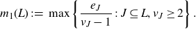 \[ m_1(L) \;:\!=\; \max \left\{ \frac{e_J}{v_J-1} \;:\; J \subseteq L, v_J \geq 2 \right\}.\]
We also make the following definition.
Definition 5·1. Given positive integers $s \leq t$
, we say that a graph is an (s,t)-graph if its minimum degree is at least s, and every edge contains a vertex of degree at least t. We say that a graph is (s,t)-avoiding if none of its subgraphs is an (s, t)-graph.
$s \leq t$
, we say that a graph is an (s,t)-graph if its minimum degree is at least s, and every edge contains a vertex of degree at least t. We say that a graph is (s,t)-avoiding if none of its subgraphs is an (s, t)-graph.
Proposition 5·2. Let $(\mathcal{H},\mathcal{L})$
be a strictly balanced pair of finite families of graphs satisfying
$(\mathcal{H},\mathcal{L})$
be a strictly balanced pair of finite families of graphs satisfying $m_2(\mathcal{H})>m_2(\mathcal{L})$
and suppose that at least one of the following conditions holds:
$m_2(\mathcal{H})>m_2(\mathcal{L})$
and suppose that at least one of the following conditions holds:
-
(a)
$\chi(L) \geq 3$
for all
$L \in \mathcal{L}$
; -
(b)
$\chi(H) \gt m_2(\mathcal{H},\mathcal{L}) + 1$
for every
$H \in \mathcal{H}$
; -
(c)
$m_1(L) \gt 2$
for all
$L \in \mathcal{L}$
; -
(d) every
$H \in \mathcal{H}$
contains an (s,t)-graph as a subgraph, for some integers
$s \leq t$
satisfying
\[ \frac{1}{s+1} + \frac{1}{t+1} \lt \frac{1}{m_2(\mathcal{H},\mathcal{L})}; \]
-
(e)
$\lceil m_2(\mathcal{H},\mathcal{L}) \rceil<m_2(\mathcal{H})$
;


Then any graph G with $m(G) \leq m_2(\mathcal{H},\mathcal{L})$
is not Ramsey for
$m(G) \leq m_2(\mathcal{H},\mathcal{L})$
is not Ramsey for $(\mathcal{H},\mathcal{L})$
.
$(\mathcal{H},\mathcal{L})$
.
Cases (a)–(c) all follow fairly easily from known colouring techniques; we supply the details in the remainder of this section. Case (d) is proved by a short inductive argument, see below. Case (e) follows from our partial progress on Conjecture 1·5, namely, that we are able to prove it when m(G) is an integer; we present the proof of this result in Appendix B. We end this section with short derivations of Theorems 1·4 and 1·7 from the proposition.
Proof of Theorem 1·4. Assume that $m_2(L)> {11}/5$
. By passing to a subgraph with the same 2-density, we may assume that L is strictly 2-balanced. Thanks to cases (a) and (c) of Proposition 5·2, we are done unless
$m_2(L)> {11}/5$
. By passing to a subgraph with the same 2-density, we may assume that L is strictly 2-balanced. Thanks to cases (a) and (c) of Proposition 5·2, we are done unless $m_1(L) \leq 2$
and L is bipartite. The bounds on
$m_1(L) \leq 2$
and L is bipartite. The bounds on $m_1(L)$
and
$m_1(L)$
and $m_2(L)$
imply that
$m_2(L)$
imply that $2v_L-2 \geq e_L \gt ({11}/5)(v_L-2)+1$
, which yields
$2v_L-2 \geq e_L \gt ({11}/5)(v_L-2)+1$
, which yields $v_L \lt 7$
. However, as L is bipartite on at most six vertices, we have
$v_L \lt 7$
. However, as L is bipartite on at most six vertices, we have $m_2(L)\leq m_2(K_{3,3})=2$
, a contradiction.
$m_2(L)\leq m_2(K_{3,3})=2$
, a contradiction.
Proof of Theorem 1·7. Cases (a), (b), (c), and (f) follow immediatelyFootnote 7 from Proposition 5·2. For Theorem 1·7(d), note that a graph with minimum degree d is a (d, d)-graph. Thus, if $H_1$
has degeneracy at least d, then it contains some (d, d)-graph as a subgraph. Similarly, Theorem 1·7(e) follows, since if
$H_1$
has degeneracy at least d, then it contains some (d, d)-graph as a subgraph. Similarly, Theorem 1·7(e) follows, since if $s \leq t$
, then
$s \leq t$
, then $K_{s,t}$
is an (s, t)-graph satisfying
$K_{s,t}$
is an (s, t)-graph satisfying $1/m_2(K_{s,t})=(s+t-2)/(st-1) \geq 1/(s+1)+1/(t+1)$
.
$1/m_2(K_{s,t})=(s+t-2)/(st-1) \geq 1/(s+1)+1/(t+1)$
.
5·1. Auxiliary results.
We start with a helpful observation relating m(G) and the degeneracy of G. We say that a graph is d-degenerate if its degeneracy is at most d.
Lemma 5·3. Every graph G is $\lfloor 2m(G) \rfloor$
-degenerate.
$\lfloor 2m(G) \rfloor$
-degenerate.
Proof. For every $G' \subseteq G$
, we have
$G' \subseteq G$
, we have
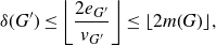 \[\delta(G') \leq \left\lfloor\frac{2e_{G'}}{v_{G'}}\right\rfloor \leq \lfloor 2m(G) \rfloor,\]
where $\delta(G')$
is the minimum degree of
$\delta(G')$
is the minimum degree of $G'\!$
.
$G'\!$
.
Our second lemma allows us to compare between the various densities.
Lemma 5·4. For every graph H, we have $m_2(H) \leq m_1(H) + {1}/{2} \leq m(H) + 1$
.
$m_2(H) \leq m_1(H) + {1}/{2} \leq m(H) + 1$
.
Proof. Notice that both ${(e-1)}/{(v-2)} \leq {e}/({v-1}) + {1}/{2}$
and
${(e-1)}/{(v-2)} \leq {e}/({v-1}) + {1}/{2}$
and ${e}/({v-1}) \leq {e}/{v} + {1}/{2}$
are equivalent to
${e}/({v-1}) \leq {e}/{v} + {1}/{2}$
are equivalent to $e \leq \binom v 2$
, so both inequalities hold whenever v, e are the numbers of vertices and edges, respectively, of any graph. In particular, if v, e correspond to the subgraph of H that achieves
$e \leq \binom v 2$
, so both inequalities hold whenever v, e are the numbers of vertices and edges, respectively, of any graph. In particular, if v, e correspond to the subgraph of H that achieves $m_2(H)$
, we find that
$m_2(H)$
, we find that $m_2(H)=({e-1})/({v-2}) \leq {e}/({v-1}) + {1}/{2} \leq m_1(H) + {1}/{2}$
. The second inequality follows in the same way, now passing to the subgraph that achieves
$m_2(H)=({e-1})/({v-2}) \leq {e}/({v-1}) + {1}/{2} \leq m_1(H) + {1}/{2}$
. The second inequality follows in the same way, now passing to the subgraph that achieves $m_1(H)$
.
$m_1(H)$
.
Our next lemma gives a lower bound on the average degree of an (s, t)-graph. We remark that this inequality is tight for $K_{s,t}$
and that it can be restated as
$K_{s,t}$
and that it can be restated as $e_H/v_H \geq m(K_{s,t})$
.
$e_H/v_H \geq m(K_{s,t})$
.
Lemma 5·5. If H is an (s,t)-graph, then
 \[\frac{1}{s} + \frac{1}{t} \geq \frac{v_H}{e_H}.\]
Proof. The assumption that H is an (s, t)-graph implies that, for every $uv \in E(H)$
, we have
$uv \in E(H)$
, we have $1/{\deg(u)} + 1/{\deg(v)} \leq 1/s + 1/t$
. This means that
$1/{\deg(u)} + 1/{\deg(v)} \leq 1/s + 1/t$
. This means that
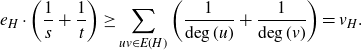 \[ e_H \cdot \left(\frac{1}{s} + \frac{1}{t}\right) \geq \sum_{uv \in E(H)} \left( \frac{1}{\deg(u)} + \frac{1}{\deg(v)}\right) = v_H. \]
The next lemma supplies a decomposition of a graph of bounded degeneracy.
Lemma 5·6. If a graph G is $(dk-1)$
-degenerate, for some positive integers d,k, then there is a partition
$(dk-1)$
-degenerate, for some positive integers d,k, then there is a partition $V(G) = V_1 \cup \dotsb \cup V_k$
such that the graphs
$V(G) = V_1 \cup \dotsb \cup V_k$
such that the graphs $G[V_1], \dotsc, G[V_k]$
are all
$G[V_1], \dotsc, G[V_k]$
are all $(d-1)$
-degenerate.
$(d-1)$
-degenerate.
Proof. We may construct the desired partition in the following way. Initialise $V_1 = \dotsb = V_k = \varnothing$
and let
$V_1 = \dotsb = V_k = \varnothing$
and let $v_1, \dotsc, v_n$
be an ordering of the vertices of G such that every
$v_1, \dotsc, v_n$
be an ordering of the vertices of G such that every $v_i$
has at most
$v_i$
has at most $dk-1$
neighbors preceding it. We distribute the vertices one-by-one, each time putting
$dk-1$
neighbors preceding it. We distribute the vertices one-by-one, each time putting $v_i$
in a set
$v_i$
in a set $V_j$
where, at the time,
$V_j$
where, at the time, $v_i$
has the smallest number of neighbors. By the pigeonhole principle, this number is at most
$v_i$
has the smallest number of neighbors. By the pigeonhole principle, this number is at most $\lfloor ({dk-1})/{k} \rfloor = d-1$
.
$\lfloor ({dk-1})/{k} \rfloor = d-1$
.
Finally, we quote Nash-Williams’s theorem on partitions of graphs into forests.
Theorem 5·7 (Nash-Williams [
Reference Nash-Williams21
]). A graph G can be partitioned into t forests if and only if $\lceil m_1(G) \rceil \leq t$
.
$\lceil m_1(G) \rceil \leq t$
.
5·2. Proof of Proposition 5·2
We are now ready to prove Proposition 5·2. Denote $\alpha \;:\!=\; m_2(\mathcal{H},\mathcal{L})$
and let G be an arbitrary graph satisfying
$\alpha \;:\!=\; m_2(\mathcal{H},\mathcal{L})$
and let G be an arbitrary graph satisfying $m(G) \leq \alpha$
. We will argue that (the edge set of) G can be partitioned into an
$m(G) \leq \alpha$
. We will argue that (the edge set of) G can be partitioned into an $\mathcal{H}$
-free graph and an
$\mathcal{H}$
-free graph and an $\mathcal{L}$
-free graph. We split into cases, depending on which condition is satisfied by the pair
$\mathcal{L}$
-free graph. We split into cases, depending on which condition is satisfied by the pair $(\mathcal{H},\mathcal{L})$
.
$(\mathcal{H},\mathcal{L})$
.
Cases (a) and (b). Let $k \;:\!=\; \lfloor \alpha \rfloor+1$
, so that
$k \;:\!=\; \lfloor \alpha \rfloor+1$
, so that $m(G) \leq \alpha \lt k$
, and note that Lemma 5·3 implies that G is
$m(G) \leq \alpha \lt k$
, and note that Lemma 5·3 implies that G is $(2k-1)$
-degenerate. Consequently, Lemma 5·6 yields two partitions of the edges of G: a partition into a 1-degenerate graph and a k-colourable graph; and a partition into a
$(2k-1)$
-degenerate. Consequently, Lemma 5·6 yields two partitions of the edges of G: a partition into a 1-degenerate graph and a k-colourable graph; and a partition into a $(k-1)$
-degenerate graph and a bipartite graph. The existence of the first partition proves (b), as every 1-degenerate graph is
$(k-1)$
-degenerate graph and a bipartite graph. The existence of the first partition proves (b), as every 1-degenerate graph is $\mathcal{L}$
-free whereas the assumption on
$\mathcal{L}$
-free whereas the assumption on $\mathcal{H}$
implies that
$\mathcal{H}$
implies that $\chi(H) \gt k$
for every
$\chi(H) \gt k$
for every $H \in \mathcal{H}$
. We now argue that the existence of the second partition proves (a). To this end, note that the assumption there implies that every bipartite graph is
$H \in \mathcal{H}$
. We now argue that the existence of the second partition proves (a). To this end, note that the assumption there implies that every bipartite graph is $\mathcal{L}$
-free, so it is enough to show that
$\mathcal{L}$
-free, so it is enough to show that $\delta(H) \geq k$
for every
$\delta(H) \geq k$
for every $H \in \mathcal{H}$
and thus every
$H \in \mathcal{H}$
and thus every $(k-1)$
-degenerate graph is
$(k-1)$
-degenerate graph is $\mathcal{H}$
-free. To see that this is the case, consider an arbitrary
$\mathcal{H}$
-free. To see that this is the case, consider an arbitrary $H \in \mathcal{H}$
and let
$H \in \mathcal{H}$
and let $v \in V(H)$
be its vertex with smallest degree. As H is strictly
$v \in V(H)$
be its vertex with smallest degree. As H is strictly $m_2(\cdot, \mathcal{L})$
-balanced, Lemma 3·5 gives
$m_2(\cdot, \mathcal{L})$
-balanced, Lemma 3·5 gives $\delta(H) = e_H - e_{H\setminus v} \gt \alpha$
, unless
$\delta(H) = e_H - e_{H\setminus v} \gt \alpha$
, unless $v_H = 3$
, in which case
$v_H = 3$
, in which case $H = K_3$
and we still have
$H = K_3$
and we still have $\delta(H) \geq 2 = m_2(H) \geq m_2(\mathcal{H}) \gt \alpha$
. Since
$\delta(H) \geq 2 = m_2(H) \geq m_2(\mathcal{H}) \gt \alpha$
. Since $\delta(H)$
is an integer, we actually have
$\delta(H)$
is an integer, we actually have $\delta(H) \geq \lfloor \alpha \rfloor+1 = k$
, as needed.
$\delta(H) \geq \lfloor \alpha \rfloor+1 = k$
, as needed.
Case (c). It is enough to show that G can be partitioned into an $\mathcal{H}$
-free graph and a union of two forests; indeed, if
$\mathcal{H}$
-free graph and a union of two forests; indeed, if $m_1(L) \gt 2$
for all
$m_1(L) \gt 2$
for all $L \in \mathcal{L}$
, then no union of two forests can contain a member of
$L \in \mathcal{L}$
, then no union of two forests can contain a member of $\mathcal{L}$
as a subgraph, by (the easy direction of) Theorem 5·7. Let
$\mathcal{L}$
as a subgraph, by (the easy direction of) Theorem 5·7. Let $m_1(\mathcal{H}) \;:\!=\; \min\{m_1(H)\;:\;H \in \mathcal{H}\}$
. By Lemma 5·4 and the assumption
$m_1(\mathcal{H}) \;:\!=\; \min\{m_1(H)\;:\;H \in \mathcal{H}\}$
. By Lemma 5·4 and the assumption $m(G) \leq m_2(\mathcal{H},\mathcal{L}) \lt m_2(\mathcal{H})$
, we find that
$m(G) \leq m_2(\mathcal{H},\mathcal{L}) \lt m_2(\mathcal{H})$
, we find that
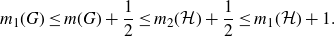 \[m_1(G) \leq m(G) + \frac{1}{2} \leq m_2(\mathcal{H}) + \frac{1}{2} \leq m_1(\mathcal{H}) + 1.\]
As a result, if we let $t \;:\!=\; \lceil m_1(\mathcal{H}) \rceil$
, we find that
$t \;:\!=\; \lceil m_1(\mathcal{H}) \rceil$
, we find that $\lceil m_1(G) \rceil \leq t+1$
and therefore Theorem 5·7 supplies a partition G into
$\lceil m_1(G) \rceil \leq t+1$
and therefore Theorem 5·7 supplies a partition G into $t+1$
forests
$t+1$
forests $G_1, \ldots ,G_{t+1}$
. Taking
$G_1, \ldots ,G_{t+1}$
. Taking $G' \;:\!=\; G_1 \cup \ldots \cup G_{t-1}$
, we arrive at a partition
$G' \;:\!=\; G_1 \cup \ldots \cup G_{t-1}$
, we arrive at a partition $G = G' \cup (G_t \cup G_{t+1})$
. By (the easy direction of) Theorem 5·7, we know that
$G = G' \cup (G_t \cup G_{t+1})$
. By (the easy direction of) Theorem 5·7, we know that $m_1(G') \leq t-1 \lt m_1(\mathcal{H})$
, so
$m_1(G') \leq t-1 \lt m_1(\mathcal{H})$
, so $G'$
is
$G'$
is $\mathcal{H}$
-free. As
$\mathcal{H}$
-free. As $G_t$
and
$G_t$
and $G_{t+1}$
are forests, we get the desired decomposition.
$G_{t+1}$
are forests, we get the desired decomposition.
Case (d). It is enough to show that G can be decomposed into a forest and an (s, t)-avoiding graph. Assume that this is not the case and let G be a smallest counterexample with $m(G) \leq \alpha$
. It is enough to show that G is an
$m(G) \leq \alpha$
. It is enough to show that G is an $(s+1,t+1)$
-graph, as then Lemma 5·5 gives
$(s+1,t+1)$
-graph, as then Lemma 5·5 gives
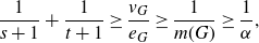 \[ \frac{1}{s+1} + \frac{1}{t+1} \geq \frac{v_G}{e_G} \geq \frac{1}{m(G)} \geq \frac{1}{\alpha},\]
a contradiction.
Suppose first that G has a vertex v of degree at most s. By minimality of G, we can decompose the edges of $G \setminus v$
into an (s, t)-avoiding graph
$G \setminus v$
into an (s, t)-avoiding graph $K$
and a forest F. Adding an arbitrary edge incident with v to F and the remaining edges to K maintains F being a forest and K being (s, t)-avoiding, as any (s, t)-subgraph of K would have to use v, which has degree at most
$K$
and a forest F. Adding an arbitrary edge incident with v to F and the remaining edges to K maintains F being a forest and K being (s, t)-avoiding, as any (s, t)-subgraph of K would have to use v, which has degree at most $s-1$
in K. This contradicts our assumption on indecomposability of G.
$s-1$
in K. This contradicts our assumption on indecomposability of G.
Second, suppose that G contains an edge uv with $\deg(u), \deg(v) \leq t$
. By minimality of G, we can decompose
$\deg(u), \deg(v) \leq t$
. By minimality of G, we can decompose $G' \;:\!=\; G\setminus uv$
into a forest F and an (s, t)-avoiding graph
$G' \;:\!=\; G\setminus uv$
into a forest F and an (s, t)-avoiding graph $K$
. Adding uv to F must close a cycle, meaning that both u and v are incident to at least one F-edge of
$K$
. Adding uv to F must close a cycle, meaning that both u and v are incident to at least one F-edge of $G'$
and thus the K-degrees of u and v in
$G'$
and thus the K-degrees of u and v in $G'$
are at most
$G'$
are at most $t-2$
. This means, however, that we can add uv to K while still keeping the degrees of both its endpoints strictly below t. Again, we find that K contains no (s, t)-subgraph, a contradiction.
$t-2$
. This means, however, that we can add uv to K while still keeping the degrees of both its endpoints strictly below t. Again, we find that K contains no (s, t)-subgraph, a contradiction.
Case (e). Let $k \;:\!=\; \lceil m_2(\mathcal{H},\mathcal{L}) \rceil$
. Since we assume that
$k \;:\!=\; \lceil m_2(\mathcal{H},\mathcal{L}) \rceil$
. Since we assume that $m_2(\mathcal{H}) \gt k$
, it is enough to decompose G into a forest and a graph
$m_2(\mathcal{H}) \gt k$
, it is enough to decompose G into a forest and a graph $K$
with
$K$
with $m_2(K) \leq k$
. The following theorem, which implies Conjecture 1·5 in the case that m(G) is an integer, supplies such a decomposition.
$m_2(K) \leq k$
. The following theorem, which implies Conjecture 1·5 in the case that m(G) is an integer, supplies such a decomposition.
Theorem 5·8. Let k be an integer, and let G be a graph with $m(G) \leq k$
. Then there exists a forest
$m(G) \leq k$
. Then there exists a forest $F \subseteq G$
such that
$F \subseteq G$
such that $m_2(G \setminus F) \leq k$
.
$m_2(G \setminus F) \leq k$
.
The proof of Theorem 5·8 is substantially more involved, as it relies on techniques from matroid theory. We are hopeful that similar techniques may be used to prove Conjecture 1·5 in its entirety. We defer the proof of Theorem 5·8 to Appendix B.
Acknowledgments
We would like to thank Anita Liebenau and Letícia Mattos for fruitful discussions on Ramsey properties of random graphs. We are also indebted to Candida Bowtell, Robert Hancock and Joseph Hyde for sharing an early draft of their paper [ Reference Bowtell, Hancock and Hyde2 ] with us, and for their many invaluable comments. Finally, we wish to thank the anonymous referee for their careful reading and helpful feedback.
Appendix A. The three-colour setting
In this section, we explain what about the proof needs to change to handle the case $r \geq 3$
, and prove Theorem 1·6. As many of these results are essentially identical to the results discussed previously, we omit or shorten several of the proofs. We begin by defining a natural three-colour analogue of cores.
$r \geq 3$
, and prove Theorem 1·6. As many of these results are essentially identical to the results discussed previously, we omit or shorten several of the proofs. We begin by defining a natural three-colour analogue of cores.
Definition A·1. Let $\mathcal{H}_1,\mathcal{H}_2,\mathcal{H}_3$
be three finite families of graphs. A tuple
$\mathcal{H}_1,\mathcal{H}_2,\mathcal{H}_3$
be three finite families of graphs. A tuple $(G,\mathcal{F}_1,\mathcal{F}_2,\mathcal{F}_3)$
is an
$(G,\mathcal{F}_1,\mathcal{F}_2,\mathcal{F}_3)$
is an $(\mathcal{H}_1,\mathcal{H}_2,\mathcal{H}_3)$
-core if G is a graph and
$(\mathcal{H}_1,\mathcal{H}_2,\mathcal{H}_3)$
-core if G is a graph and $\mathcal{F}_i \subseteq \mathcal{F}_{\mathcal{H}_i}[G]$
for all
$\mathcal{F}_i \subseteq \mathcal{F}_{\mathcal{H}_i}[G]$
for all $i \in [\![{3}]\!]$
are families satisfying the following properties:
$i \in [\![{3}]\!]$
are families satisfying the following properties:
-
(1) the hypergraph
$\mathcal{F}_{1} \cup \mathcal{F}_{2} \cup \mathcal{F}_{3}$
is connected and spans E(G); -
(ii) for every
$i \in [\![{3}]\!]$
, every
$\widehat{H_i} \in \mathcal{F}_i$
, every edge
$e \in \widehat{H_i}$
, and every
$j \in [\![{3}]\!] \setminus \{i\}$
, there is some
$\widehat{H_j} \in \mathcal{F}_j$
with
$\widehat{H_i} \cap \widehat{H_j} = \{e\}$
.


We say that G supports a core if there exists a core $(G,\mathcal{F}_1,\mathcal{F}_2,\mathcal{F}_3)$
.
$(G,\mathcal{F}_1,\mathcal{F}_2,\mathcal{F}_3)$
.
The following simple lemma is a straightforward generalisation of Lemma 3·2, so we omit the proof.
Lemma A·2. Let G be a graph that is minimally Ramsey for $(\mathcal{H}_1,\mathcal{H}_2,\mathcal{H}_3)$
, in the sense that any proper subgraph
$(\mathcal{H}_1,\mathcal{H}_2,\mathcal{H}_3)$
, in the sense that any proper subgraph $G' \subsetneq G$
is not Ramsey for
$G' \subsetneq G$
is not Ramsey for $(\mathcal{H}_1,\mathcal{H}_2,\mathcal{H}_3)$
. Then G supports a core.
$(\mathcal{H}_1,\mathcal{H}_2,\mathcal{H}_3)$
. Then G supports a core.
It would be very convenient if every $(\mathcal{H}_1,\mathcal{H}_2,\mathcal{H}_3)$
-core were also an
$(\mathcal{H}_1,\mathcal{H}_2,\mathcal{H}_3)$
-core were also an $(\mathcal{H}_1,\mathcal{H}_2)$
-core. At first glance this seems true, since the intersection property in Definition A·1 core easily implies the intersection property in Definition 3·1. Unfortunately, it may be the case that the hypergraph
$(\mathcal{H}_1,\mathcal{H}_2)$
-core. At first glance this seems true, since the intersection property in Definition A·1 core easily implies the intersection property in Definition 3·1. Unfortunately, it may be the case that the hypergraph $\mathcal{F}_1 \cup \mathcal{F}_2 \cup \mathcal{F}_3$
is connected, but that the hypergraph
$\mathcal{F}_1 \cup \mathcal{F}_2 \cup \mathcal{F}_3$
is connected, but that the hypergraph $\mathcal{F}_1 \cup \mathcal{F}_2$
is disconnected. Nonetheless, this is the only obstruction, and the following result is true.
$\mathcal{F}_1 \cup \mathcal{F}_2$
is disconnected. Nonetheless, this is the only obstruction, and the following result is true.
Lemma A·3. Let $(G,\mathcal{F}_1,\mathcal{F}_2,\mathcal{F}_3)$
be
$(G,\mathcal{F}_1,\mathcal{F}_2,\mathcal{F}_3)$
be $(\mathcal{H}_1,\mathcal{H}_2,\mathcal{H}_3)$
-core for some families of graphs
$(\mathcal{H}_1,\mathcal{H}_2,\mathcal{H}_3)$
-core for some families of graphs $\mathcal{H}_1,\mathcal{H}_2,\mathcal{H}_3$
. Then
$\mathcal{H}_1,\mathcal{H}_2,\mathcal{H}_3$
. Then $(G,\mathcal{F}_1,\mathcal{F}_2 \cup \mathcal{F}_3)$
is an
$(G,\mathcal{F}_1,\mathcal{F}_2 \cup \mathcal{F}_3)$
is an $(\mathcal{H}_1,\mathcal{H}_2 \cup \mathcal{H}_3)$
-core.
$(\mathcal{H}_1,\mathcal{H}_2 \cup \mathcal{H}_3)$
-core.
Proof. First note that the hypergraph $\mathcal{F}_1 \cup (\mathcal{F}_2 \cup \mathcal{F}_3)$
is simply the same as the hypergraph
$\mathcal{F}_1 \cup (\mathcal{F}_2 \cup \mathcal{F}_3)$
is simply the same as the hypergraph $\mathcal{F}_1 \cup \mathcal{F}_2 \cup \mathcal{F}_3$
, so it is connected and spans E(G) by assumption. For every
$\mathcal{F}_1 \cup \mathcal{F}_2 \cup \mathcal{F}_3$
, so it is connected and spans E(G) by assumption. For every $\widehat{H_1} \in \mathcal{F}_1$
and every edge
$\widehat{H_1} \in \mathcal{F}_1$
and every edge $e \in \widehat{H_1}$
, we may apply Definition A·1 with
$e \in \widehat{H_1}$
, we may apply Definition A·1 with $j=2$
to see that there exists some
$j=2$
to see that there exists some $\widehat{H_2} \in \mathcal{F}_2 \subseteq \mathcal{F}_2 \cup \mathcal{F}_3$
such that
$\widehat{H_2} \in \mathcal{F}_2 \subseteq \mathcal{F}_2 \cup \mathcal{F}_3$
such that $\widehat{H_1} \cap \widehat{H_2} = \{e\}$
. Similarly, applying Definition A·1 with
$\widehat{H_1} \cap \widehat{H_2} = \{e\}$
. Similarly, applying Definition A·1 with $j=1$
, we see that for every
$j=1$
, we see that for every $\widehat{H_{23}} \in \mathcal{F}_2 \cup \mathcal{F}_3$
and every edge
$\widehat{H_{23}} \in \mathcal{F}_2 \cup \mathcal{F}_3$
and every edge $e \in \widehat{H_{23}}$
, there is some
$e \in \widehat{H_{23}}$
, there is some $\widehat{H_1} \in \mathcal{F}_1$
such that
$\widehat{H_1} \in \mathcal{F}_1$
such that $\widehat{H_1} \cap \widehat{H_{23}} = \{e\}$
. Thus,
$\widehat{H_1} \cap \widehat{H_{23}} = \{e\}$
. Thus, $(G,\mathcal{F}_1,\mathcal{F}_2 \cup \mathcal{F}_3)$
is an
$(G,\mathcal{F}_1,\mathcal{F}_2 \cup \mathcal{F}_3)$
is an $(\mathcal{H}_1,\mathcal{H}_2 \cup \mathcal{H}_3)$
-core.
$(\mathcal{H}_1,\mathcal{H}_2 \cup \mathcal{H}_3)$
-core.
The key (trivial) observation is that if $m_2(\mathcal{H}_2) = m_2(\mathcal{H}_3)$
, then
$m_2(\mathcal{H}_2) = m_2(\mathcal{H}_3)$
, then $m_2(\mathcal{H}_2 \cup \mathcal{H}_3)$
is also equal to both these numbers, as
$m_2(\mathcal{H}_2 \cup \mathcal{H}_3)$
is also equal to both these numbers, as $m_2(\mathcal{H}_2 \cup \mathcal{H}_3) = \min \{m_2(\mathcal{H}_2),m_2(\mathcal{H}_3)\}$
. Now, suppose we are given families
$m_2(\mathcal{H}_2 \cup \mathcal{H}_3) = \min \{m_2(\mathcal{H}_2),m_2(\mathcal{H}_3)\}$
. Now, suppose we are given families $\mathcal{H}_1,\mathcal{H}_2,\mathcal{H}_3$
with
$\mathcal{H}_1,\mathcal{H}_2,\mathcal{H}_3$
with $m_2(\mathcal{H}_1)>m_2(\mathcal{H}_2)=m_2(\mathcal{H}_3)$
. By passing to families of subgraphs, we may assume that
$m_2(\mathcal{H}_1)>m_2(\mathcal{H}_2)=m_2(\mathcal{H}_3)$
. By passing to families of subgraphs, we may assume that $\mathcal{H}_2,\mathcal{H}_3$
are strictly 2-balanced and that
$\mathcal{H}_2,\mathcal{H}_3$
are strictly 2-balanced and that $\mathcal{H}_1$
is strictly
$\mathcal{H}_1$
is strictly $m_2(\cdot,\mathcal{H}_2)$
-balanced. We now define
$m_2(\cdot,\mathcal{H}_2)$
-balanced. We now define $\mathcal{H}=\mathcal{H}_1$
and
$\mathcal{H}=\mathcal{H}_1$
and $\mathcal{L}=\mathcal{H}_2 \cup \mathcal{H}_3$
. By Lemma 4·1, we know that there exists some
$\mathcal{L}=\mathcal{H}_2 \cup \mathcal{H}_3$
. By Lemma 4·1, we know that there exists some $c>0$
such that if
$c>0$
such that if $p \leq cn^{-1/m_2(\mathcal{H},\mathcal{L})}$
, then a.a.s.
$p \leq cn^{-1/m_2(\mathcal{H},\mathcal{L})}$
, then a.a.s. $G_{n,p}$
contains no subgraph G which supports an
$G_{n,p}$
contains no subgraph G which supports an $(\mathcal{H},\mathcal{L})$
-core and satisfies
$(\mathcal{H},\mathcal{L})$
-core and satisfies $m(G) \gt m_2(\mathcal{H},\mathcal{L})$
.
$m(G) \gt m_2(\mathcal{H},\mathcal{L})$
.
On the other hand, if $G_{n,p}$
is Ramsey for
$G_{n,p}$
is Ramsey for $(\mathcal{H}_1,\mathcal{H}_2,\mathcal{H}_3)$
, then it must contain some minimally Ramsey subgraph G. By Lemmas A·2 and A·3, G supports an
$(\mathcal{H}_1,\mathcal{H}_2,\mathcal{H}_3)$
, then it must contain some minimally Ramsey subgraph G. By Lemmas A·2 and A·3, G supports an $(\mathcal{H},\mathcal{L})$
-core. Moreover, by the above, we must have
$(\mathcal{H},\mathcal{L})$
-core. Moreover, by the above, we must have $m(G) \leq m_2(\mathcal{H},\mathcal{L}) = m_2(\mathcal{H}_1,\mathcal{H}_2)$
, for otherwise
$m(G) \leq m_2(\mathcal{H},\mathcal{L}) = m_2(\mathcal{H}_1,\mathcal{H}_2)$
, for otherwise $G \nsubseteq G_{n,p}$
a.a.s. Given this, the following deterministic lemma concludes the proof.
$G \nsubseteq G_{n,p}$
a.a.s. Given this, the following deterministic lemma concludes the proof.
Lemma A·4. Let $\mathcal{H}_1,\mathcal{H}_2,\mathcal{H}_3$
satisfy
$\mathcal{H}_1,\mathcal{H}_2,\mathcal{H}_3$
satisfy $m(\mathcal{H}_1) \geq m(\mathcal{H}_2) \geq m(\mathcal{H}_3)>1$
. If G is Ramsey for
$m(\mathcal{H}_1) \geq m(\mathcal{H}_2) \geq m(\mathcal{H}_3)>1$
. If G is Ramsey for $(\mathcal{H}_1,\mathcal{H}_2,\mathcal{H}_3)$
, then
$(\mathcal{H}_1,\mathcal{H}_2,\mathcal{H}_3)$
, then $m(G) \gt m_2(\mathcal{H}_1,\mathcal{H}_2)$
.
$m(G) \gt m_2(\mathcal{H}_1,\mathcal{H}_2)$
.
Proof. We will actually prove that $m(G) \gt m_2(\mathcal{H}_1)$
, which implies the desired result since
$m(G) \gt m_2(\mathcal{H}_1)$
, which implies the desired result since $m_2(\mathcal{H}_1) \geq m_2(\mathcal{H}_1,\mathcal{H}_2)$
. Suppose for contradiction that
$m_2(\mathcal{H}_1) \geq m_2(\mathcal{H}_1,\mathcal{H}_2)$
. Suppose for contradiction that $m(G) \leq m_2(\mathcal{H}_1)$
. By Theorem 5·7 (cf. the proof of Proposition 5·2(c)), we know that G is the union of an
$m(G) \leq m_2(\mathcal{H}_1)$
. By Theorem 5·7 (cf. the proof of Proposition 5·2(c)), we know that G is the union of an $\mathcal{H}_1$
-free graph and two forests. As
$\mathcal{H}_1$
-free graph and two forests. As $m_2(\mathcal{H}_2) \geq m_2(\mathcal{H}_3)>1$
, every graph in
$m_2(\mathcal{H}_2) \geq m_2(\mathcal{H}_3)>1$
, every graph in $\mathcal{H}_2 \cup \mathcal{H}_3$
contains a cycle, and hence each of these forests is
$\mathcal{H}_2 \cup \mathcal{H}_3$
contains a cycle, and hence each of these forests is $\mathcal{H}_2 \cup \mathcal{H}_3$
-free. Using one colour for the
$\mathcal{H}_2 \cup \mathcal{H}_3$
-free. Using one colour for the $\mathcal{H}_1$
-free graph and one colour for each of the two forests, we see that G is not Ramsey for
$\mathcal{H}_1$
-free graph and one colour for each of the two forests, we see that G is not Ramsey for $(\mathcal{H}_1,\mathcal{H}_2,\mathcal{H}_3)$
.
$(\mathcal{H}_1,\mathcal{H}_2,\mathcal{H}_3)$
.
Appendix B. Proof of Conjecture 1·5 in the integer case
In this section, we present the proof of Theorem 5·8, which implies Conjecture 1·5 in the case that m(G) is an integer. We will use some well-known results from matroid theory; all definitions and proofs can be found in any standard reference on matroid theory, such as Oxley’s book [ Reference Oxley23 ].
The main result we will need is the following matroid partitioning theorem, originally due to Edmonds [ Reference Edmonds5 ]. We remark that this theorem easily implies Nash–Williams’s theorem (Theorem 5·7), which was used in the proof of Proposition 5·2(c).
Theorem B·1. Let $M_1,M_2$
be matroids on the same ground set E, with rank functions
$M_1,M_2$
be matroids on the same ground set E, with rank functions $r_1,r_2$
, respectively. Then E can be partitioned as
$r_1,r_2$
, respectively. Then E can be partitioned as $E=I_1 \cup I_2$
, with
$E=I_1 \cup I_2$
, with $I_i$
independent in
$I_i$
independent in $M_i$
for
$M_i$
for $i=1,2$
, if and only if
$i=1,2$
, if and only if
 \[ r_1(X) + r_2(X) \geq \lvert X\rvert \]
for every $X \subseteq E$
.
$X \subseteq E$
.
A slightly weaker statement appears as [
Reference Oxley23
, Theorem 11·3·12], where the result is only stated when $M_1=M_2$
. However, it is clear and well known that the same proof proves Theorem B·1, using the formula for the rank of a matroid union, as given in [
Reference Oxley23
, Theorem 11·3·1].
$M_1=M_2$
. However, it is clear and well known that the same proof proves Theorem B·1, using the formula for the rank of a matroid union, as given in [
Reference Oxley23
, Theorem 11·3·1].
In our application, we will set $E=E(G)$
and let
$E=E(G)$
and let $M_1$
be the graphic matroid of G, whose independent sets are precisely the acyclic subgraphs of G. We may view any subset of E(G) as a subgraph J of G; we then use
$M_1$
be the graphic matroid of G, whose independent sets are precisely the acyclic subgraphs of G. We may view any subset of E(G) as a subgraph J of G; we then use $e_J$
rather than
$e_J$
rather than $\lvert J\rvert$
to denote the size of this subset of E(G). Additionally, we use
$\lvert J\rvert$
to denote the size of this subset of E(G). Additionally, we use $v_J$
to denote the number of vertices incident to any edge of J, and
$v_J$
to denote the number of vertices incident to any edge of J, and $\omega_J$
to denote the number of connected components of J. It is well-known (e.g. [
Reference Oxley23
, equation 1·3·8]) that the rank function of
$\omega_J$
to denote the number of connected components of J. It is well-known (e.g. [
Reference Oxley23
, equation 1·3·8]) that the rank function of $M_1$
is given by
$M_1$
is given by $r_1(J) = v_J - \omega_J$
for all
$r_1(J) = v_J - \omega_J$
for all $J \subseteq E(G)$
.
$J \subseteq E(G)$
.
The second matroid we use will be one whose independent sets are precisely those subgraphs $K \subseteq G$
with
$K \subseteq G$
with $m_2(K) \leq k$
. The fact that this is a matroid is the content of the next lemma.
$m_2(K) \leq k$
. The fact that this is a matroid is the content of the next lemma.
Lemma B·2. Let G be a graph and let k be a positive integer. Then the family of subgraphs $K \subseteq G$
with
$K \subseteq G$
with $m_2(K) \leq k$
is the collection of independent sets of a matroid.
$m_2(K) \leq k$
is the collection of independent sets of a matroid.
Proof. Define a function $f\colon 2^{E(G)} \to \mathbb{Z}$
by
$f\colon 2^{E(G)} \to \mathbb{Z}$
by $f(J) = k(v_J-2)+1$
, for every
$f(J) = k(v_J-2)+1$
, for every $J \subseteq E(G)$
. Note that this function is integer-valued since
$J \subseteq E(G)$
. Note that this function is integer-valued since $k \in \mathbb{Z}$
. Additionally, it is clear that f is increasing, in the sense that
$k \in \mathbb{Z}$
. Additionally, it is clear that f is increasing, in the sense that $f(J) \leq f(J')$
whenever
$f(J) \leq f(J')$
whenever $J \subseteq J'$
. Finally, we claim that f is submodular. This is easiest to see by recalling that the function
$J \subseteq J'$
. Finally, we claim that f is submodular. This is easiest to see by recalling that the function $g(J) =v_J$
is submodular (see e.g. [
Reference Oxley23
, Proposition 11·1·6]); as f is obtained from g by multiplying by a positive constant and adding a constant, we find that f is submodular as well.
$g(J) =v_J$
is submodular (see e.g. [
Reference Oxley23
, Proposition 11·1·6]); as f is obtained from g by multiplying by a positive constant and adding a constant, we find that f is submodular as well.
Now, by [
Reference Oxley23
, Corollary 11·1·2], we find that there exists a matroid M(f) on E(G) whose independent sets are precisely those $K \subseteq E(G)$
with the property that
$K \subseteq E(G)$
with the property that $e_{J} \leq f({J})$
for all non-empty
$e_{J} \leq f({J})$
for all non-empty $J \subseteq K$
. Note that, for a graph
$J \subseteq K$
. Note that, for a graph $J$
with at least three vertices, the inequality
$J$
with at least three vertices, the inequality $e_{J} \leq f(J)$
is equivalent to
$e_{J} \leq f(J)$
is equivalent to $d_2(J) \leq k$
, where
$d_2(J) \leq k$
, where $d_2(J)=(e_{J}-1)/(v_{J}-2)$
. If J is non-empty and has only two vertices, then it must have one edge and
$d_2(J)=(e_{J}-1)/(v_{J}-2)$
. If J is non-empty and has only two vertices, then it must have one edge and $e_{J} \leq f(J)$
always holds. Thus, we see that K is independent in M(f) if and only if
$e_{J} \leq f(J)$
always holds. Thus, we see that K is independent in M(f) if and only if $\max \{(e_{J}-1)/(v_{J}-2) \;:\;J \subseteq K, v_{J}\geq 3\} \leq k$
. This condition is precisely the condition that
$\max \{(e_{J}-1)/(v_{J}-2) \;:\;J \subseteq K, v_{J}\geq 3\} \leq k$
. This condition is precisely the condition that $m_2(K) \leq k$
.
$m_2(K) \leq k$
.
In order to apply Theorem B·1 to the matroids $M_1,M_2$
, we need a way of lower-bounding the rank function of
$M_1,M_2$
, we need a way of lower-bounding the rank function of $M_2$
. This is achieved by the following lemma.
$M_2$
. This is achieved by the following lemma.
Lemma B·3. Let k be a positive integer. If J is a graph with $m(J) \leq k$
, then there is a subgraph
$m(J) \leq k$
, then there is a subgraph $J' \subseteq J$
with
$J' \subseteq J$
with $m_2(J') \leq k$
and
$m_2(J') \leq k$
and $e_J \leq e_{J'} + v_J- 1.$
Proof. A well-known theorem of Hakimi [
Reference Hakimi10
], which is itself a simple consequence of Theorem B·1, implies that since $m(J) \leq k$
, we can partition J into graphs
$m(J) \leq k$
, we can partition J into graphs $J_1,\ldots,J_k$
, with
$J_1,\ldots,J_k$
, with $m(J_i) \leq 1$
for all i (i.e. every component of every
$m(J_i) \leq 1$
for all i (i.e. every component of every $J_i$
has at most one cycle). We may assume without loss of generality that
$J_i$
has at most one cycle). We may assume without loss of generality that $J_k$
is non-empty. Let e be an edge of
$J_k$
is non-empty. Let e be an edge of $J_k$
and define
$J_k$
and define $J' = J_1 \cup \dotsb \cup J_{k-1} \cup \{ e\}$
. We claim that
$J' = J_1 \cup \dotsb \cup J_{k-1} \cup \{ e\}$
. We claim that $m_2(J') \leq k$
and
$m_2(J') \leq k$
and $e_{J} \leq e_{J'} + v_J -1$
.
$e_{J} \leq e_{J'} + v_J -1$
.
The second claim is fairly easy to see, as
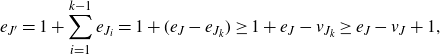 \[ e_{J'} =1+ \sum_{i=1}^{k-1} e_{J_i} = 1+(e_J - e_{J_k}) \geq 1+e_J - v_{J_k} \geq e_J - v_J +1, \]
where the second equality uses the fact that $J_1,\ldots,J_k$
partition J, and the two inequalities follow from
$J_1,\ldots,J_k$
partition J, and the two inequalities follow from $e_{J_k} \leq v_{J_k} \leq v_J$
, since
$e_{J_k} \leq v_{J_k} \leq v_J$
, since $m(J_k) \leq 1$
and
$m(J_k) \leq 1$
and $J_k \subseteq J$
.
$J_k \subseteq J$
.
So it remains to prove that $m_2(J') \leq k$
, i.e. that
$m_2(J') \leq k$
, i.e. that $d_2(L) \leq k$
for all
$d_2(L) \leq k$
for all $L \subseteq J'$
. If
$L \subseteq J'$
. If $v_{L} \leq 2k-1$
, then
$v_{L} \leq 2k-1$
, then
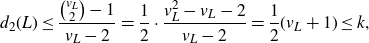 \[ d_2(L) \leq \frac{\binom{v_{L}}2-1}{v_{L}-2}=\frac 12 \cdot\frac{v_L^2-v_L-2}{v_L-2} = \frac 12 (v_L+1) \leq k, \]
as claimed. So we may assume that $v_L \geq 2k$
. As
$v_L \geq 2k$
. As $m(J_i) \leq 1$
for all i, we see that
$m(J_i) \leq 1$
for all i, we see that $e_{L} \leq (k-1)v_{L}+1$
. Therefore,
$e_{L} \leq (k-1)v_{L}+1$
. Therefore,
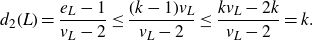 \[ d_2(L) = \frac{e_{L}-1}{v_{L}-2} \leq \frac{(k-1)v_{L}}{v_{L}-2} \leq \frac{kv_L -2k}{v_L-2} = k. \]
With all of these preliminaries, we are ready to prove Theorem 5·8.
Proof of Theorem 5·8. Let G be a graph with $m(G) \leq k$
and let
$m(G) \leq k$
and let $E=E(G)$
. Let
$E=E(G)$
. Let $M_1$
be the graphic matroid on the ground set E and let
$M_1$
be the graphic matroid on the ground set E and let $M_2$
be the matroid given by Lemma B·2, whose independent sets are those
$M_2$
be the matroid given by Lemma B·2, whose independent sets are those $K \subseteq G$
with
$K \subseteq G$
with $m_2(K) \leq k$
. We wish to prove that E can be partitioned into an independent set from
$m_2(K) \leq k$
. We wish to prove that E can be partitioned into an independent set from $M_1$
and an independent set from
$M_1$
and an independent set from $M_2$
; by Theorem B·1, it suffices to prove that
$M_2$
; by Theorem B·1, it suffices to prove that $r_1(J) + r_2(J) \geq e_J$
for all
$r_1(J) + r_2(J) \geq e_J$
for all $J \subseteq G$
.
$J \subseteq G$
.
So fix some $J \subseteq G$
, and let its connected components be
$J \subseteq G$
, and let its connected components be $J_1,\ldots,J_t$
. We then have that
$J_1,\ldots,J_t$
. We then have that $r_1(J) = v_J-\omega_J = v_J-t$
. As
$r_1(J) = v_J-\omega_J = v_J-t$
. As $m(G) \leq k$
, we certainly have that
$m(G) \leq k$
, we certainly have that $m(J_i) \leq k$
for all i, and hence Lemma B·3 implies that there exist
$m(J_i) \leq k$
for all i, and hence Lemma B·3 implies that there exist $J'_i \subseteq J_i$
with
$J'_i \subseteq J_i$
with $m_2(J'_i) \leq k$
and
$m_2(J'_i) \leq k$
and $e_{J_i} \leq e_{J'_i}+v_{J_i}-1$
. Let
$e_{J_i} \leq e_{J'_i}+v_{J_i}-1$
. Let $J' = J_1' \cup \dotsb \cup J_t'$
. If
$J' = J_1' \cup \dotsb \cup J_t'$
. If $J'$
is a matching, then
$J'$
is a matching, then $m_2(J') \leq 1 \leq k$
. If not, then its maximal 2-density is attained on some connected component, hence
$m_2(J') \leq 1 \leq k$
. If not, then its maximal 2-density is attained on some connected component, hence $m_2(J') = \max_i m_2(J_i') \leq k$
. Therefore,
$m_2(J') = \max_i m_2(J_i') \leq k$
. Therefore, $J'$
is independent in
$J'$
is independent in $M_2$
, which implies that
$M_2$
, which implies that
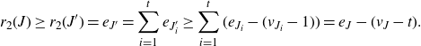 \[ r_2(J) \geq r_2(J') = e_{J'} =\sum_{i=1}^t e_{J_i'} \geq \sum_{i=1}^t (e_{J_i} - (v_{J_i}-1)) = e_J - (v_J-t). \]
Recalling that $r_1(J) = v_J-t$
, we conclude that
$r_1(J) = v_J-t$
, we conclude that $r_1(J) + r_2(J) \geq e_J$
, as claimed.
$r_1(J) + r_2(J) \geq e_J$
, as claimed.


 Open access