


1. Introduction
Understanding the immiscible fluid flows in fractured rock formations is critical for various geotechnical applications, including water resources management (De Dios et al. Reference De Dios, Delgado, Martínez, Ramos, lvarez, Iñaki, Juan and Salvador2017; Ren et al. Reference Ren, Ma, Wang, Fan and Zhu2017), environmental protection (Bikkina et al. Reference Bikkina, Wan, Kim, Kneafsey and Tokunaga2016; Zhang et al. Reference Zhang, Li, Adenutsi and Lai2017) and energy storage (Kim et al. Reference Kim, Kwon, Sanchez and Cho2011; Meng, Liu & Wang Reference Meng, Liu and Wang2017). These processes frequently involve the displacement of a wetting fluid by a non-wetting fluid, also referred to as drainage, within fractured media. Prominent examples include the displacement of brine by supercritical CO2 during carbon capture and storage (Miocic et al. Reference Miocic, Gilfillan, Roberts, Edlmann, McDermott and Haszeldine2016) and the migration of pressurised gases through water-saturated materials in nuclear waste repositories (Muller et al. Reference Muller, Finsterle, Grimsich, Baltzer, Muller, Rector, Payer and Apps2019). To support effective planning and risk assessment, accurate models of these flow processes are necessary, which are capable of predicting flow velocities and spatial fluid distributions. While two-phase flows in porous media have been extensively studied over the past two decades, fewer studies have focused specifically on this dynamics within geological fractures.
Immiscible displacements in open rough-walled fractures can be subject to different types of flow instabilities, driven by density or viscosity contrasts between the two fluids, and capillary forces also play an important role in allowing fluid-fluid interfaces to more easily invade large (respectively, small) aperture areas when the wetting fluid is the displaced (respectively, displacing) fluid (Glass et al. Reference Glass, Nicholl and Yarrington1998, Reference Glass, Rajaram and Detwiler2003; Detwiler, Rajaram & Glass Reference Detwiler, Rajaram and Glass2009). The relative magnitudes of gravity, viscous and capillary forces are typically estimated in terms of the capillary number $Ca$
(typical ratio of the viscous forces to the capillary forces), the Bond number
$Ca$
(typical ratio of the viscous forces to the capillary forces), the Bond number $Bo$
(typical ratio of the gravitational force to the capillary forces), and the ratio of the two fluids’ viscosities,
$Bo$
(typical ratio of the gravitational force to the capillary forces), and the ratio of the two fluids’ viscosities, $M$
. To properly capture the effect of all these forces in a model is challenging. Additionally, molecular-scale phenomena, including thin wetting films and moving contact lines, are challenging to model accurately (Meakin & Tartakovsky Reference Meakin and Tartakovsky2009; Krishna, Méheust & Neuweiler Reference Krishna, Méheust and Neuweiler2024).
$M$
. To properly capture the effect of all these forces in a model is challenging. Additionally, molecular-scale phenomena, including thin wetting films and moving contact lines, are challenging to model accurately (Meakin & Tartakovsky Reference Meakin and Tartakovsky2009; Krishna, Méheust & Neuweiler Reference Krishna, Méheust and Neuweiler2024).
In applications, flow processes need to be considered over large length scales in the range of tens to hundreds of metres. Yet, when flow instabilities are present, large-scale flow patterns may be impacted by small-scale properties or processes, in particular the properties of the fractures’ aperture fields. Fracture surfaces, either artificial, or in natural environments such as the subsurface, exhibit self-affine scaling behaviour, with Hurst exponents typically ranging between 0.5 and 0.8 (Bouchaud, Lapasset & Planès Reference Bouchaud, Lapasset and Planès1990; Schmittbuhl, Schmitt & Scholz Reference Schmittbuhl, Schmitt and Scholz1995; Boffa, Allain & Hulin Reference Boffa, Allain and Hulin1998), and matching of the wall topographies with each other over a characteristic correlation scale (Brown Reference Brown1995). The span of relevant length scales is thus very large.
To model the drainage process using direct numerical simulation (DNS), the Navier–Stokes equations, coupled with an interface capturing or tracking technique, are solved numerically. Although large viscosity and density ratios (Meakin & Tartakovsky Reference Meakin and Tartakovsky2009), as well as a large range of capillary numbers (Chen et al. Reference Chen, Guo, Wu and Hu2018; Krishna et al. Reference Krishna, Méheust and Neuweiler2024), can be captured, the computational cost of DNS of immiscible two-phase flow, in particular if wetting films need to be resolved, can become very large, as discussed in Krishna et al. (Reference Krishna, Méheust and Neuweiler2024) for fracture geometries, or Horgue et al. (Reference Horgue, Augier, Quintard and Prat2012) for porous media. Particle methods such as lattice Boltzmann methods (Dou, Zhou & Sleep Reference Dou, Zhou and Sleep2013; Guiltinan et al. Reference Guiltinan, Santos, Cardenas, Espinoza and Kang2021), and Lagrangian mesh-free methods such as smoothed particle hydrodynamics (Tartakovsky & Meakin Reference Tartakovsky and Meakin2005), which also provide hydrodynamic-scale resolution and respect conservation principles (Lee & Lin Reference Lee and Lin2005), are also potentially capable of handling a wide range of $Ca$
,
$Ca$
, $Bo$
and
$Bo$
and $M$
values. However, these methods encounter challenges in relating the model parameters and the underlying physics of the modelled fluid flow (Porter et al. Reference Porter, Coon, Kang, Moulton and Carey2012).
$M$
values. However, these methods encounter challenges in relating the model parameters and the underlying physics of the modelled fluid flow (Porter et al. Reference Porter, Coon, Kang, Moulton and Carey2012).
The computational demand for models accounting for the entire range of physical phenomena at play can be very large. Simplified models have been derived for flow in fractures, in particular for restricted flow regimes. Invasion percolation schemes, able to describe quasi-static fluid–fluid interface displacement controlled entirely by capillary forces, have been adapted from porous media to fracture geometries to address regimes of very slow displacements (i.e. very small $Ca$
) (Glass, Nicholl & Yarrington Reference Glass, Nicholl and Yarrington1998; Neuweiler, Sorensen & Kinzelbach Reference Neuweiler, Sorensen and Kinzelbach2004; Yang et al. Reference Yang, Niemi, Fagerlund and Illangasekare2012, Reference Yang, Neuweiler, Méheust, Fagerlund and Niemi2016). A few attempts have also been made to simulate two-phase flow in single fracture using pore network models; they have proven to be computationally efficient (Hughes & Blunt Reference Hughes and Blunt2001; Ferer et al. Reference Ferer, Crandall, Ahmadi and Smith2011), but it is difficult with this approach to properly model the in-plane component of the capillary pressure at fluid-fluid interfaces. More recently, a very efficient model was proposed to describe flow conditions for which viscous forces are the dominant displacement driver (Yang et al. Reference Yang, Méheust, Neuweiler, Hu, Niemi and Chen2019), with a single fluid–fluid interface. Another approach to flows over large scales is to consider volume-averaged upscaled models. This approach is used extensively to simulate large-scale two-phase flow in porous media (e.g. reservoir simulations), however, such models are non-local and provide convincing predictions only for restricted flow regimes (see e.g. Picchi & Battiato Reference Picchi and Battiato2018), with no interface instabilities, and are not well-suited to address media with multiscale properties, such as fracture geometries.
$Ca$
) (Glass, Nicholl & Yarrington Reference Glass, Nicholl and Yarrington1998; Neuweiler, Sorensen & Kinzelbach Reference Neuweiler, Sorensen and Kinzelbach2004; Yang et al. Reference Yang, Niemi, Fagerlund and Illangasekare2012, Reference Yang, Neuweiler, Méheust, Fagerlund and Niemi2016). A few attempts have also been made to simulate two-phase flow in single fracture using pore network models; they have proven to be computationally efficient (Hughes & Blunt Reference Hughes and Blunt2001; Ferer et al. Reference Ferer, Crandall, Ahmadi and Smith2011), but it is difficult with this approach to properly model the in-plane component of the capillary pressure at fluid-fluid interfaces. More recently, a very efficient model was proposed to describe flow conditions for which viscous forces are the dominant displacement driver (Yang et al. Reference Yang, Méheust, Neuweiler, Hu, Niemi and Chen2019), with a single fluid–fluid interface. Another approach to flows over large scales is to consider volume-averaged upscaled models. This approach is used extensively to simulate large-scale two-phase flow in porous media (e.g. reservoir simulations), however, such models are non-local and provide convincing predictions only for restricted flow regimes (see e.g. Picchi & Battiato Reference Picchi and Battiato2018), with no interface instabilities, and are not well-suited to address media with multiscale properties, such as fracture geometries.
Another approach to improve the efficiency of numerical models while considering the whole variety of physical processes at play, is to reduce the dimensionality of the model. In fracture geometries this can be done by depth integration, i.e. integrating the flow equations over the direction perpendicular to the mean fracture plane. Physical effects that may no longer be accounted for explicitly, as the third dimension is not explicitly resolved, are then captured by effective terms or parameters that are derived in the course of the depth integration. For instance, the Reynolds equation has been widely used to simulate stationary single-phase flow in rough fractures (Brown, Stockman & Reeves Reference Brown, Stockman and Reeves1995; Zimmerman & Yeo Reference Zimmerman and Yeo2000; Méheust & Schmittbuhl Reference Méheust and Schmittbuhl2001; He et al. Reference He, Sinan, Kwak and Hoteit2021). It combines the conservation of the fluid mass and the local cubic law, which states that the relation between the local flux (i.e. velocity integrated over the fracture aperture) and the pressure gradient is identical to that relating the global flow rate per transverse unit length to the macroscopic pressure gradient in a parallel plate (i.e. planar) fracture. The local cubic law can be rigorously derived from the stationary Stokes equation under the lubrication approximation, which assumes that the gradient of the fracture’s aperture field is much smaller than 1 everywhere (see, e.g. Zimmerman & Yeo Reference Zimmerman and Yeo2000). More general depth integrations of the Navier–Stokes equations over flow domains with a uniform aperture have been proposed for (i) single-phase flow in Hele-Shaw cell geometries, coupled to heat transport (Letelier, Mujica & Ortega Reference Letelier, Mujica and Ortega2019), miscible fluid mixing (Letelier et al. Reference Letelier, Ulloa, Leyrer and Ortega2023) and solute-actuated natural convection (De Paoli et al. Reference De Paoli, Alipour and Soldati2020; De et al. Reference De, Meunier, Méheust and Nadal2021), (ii) single-phase flow in two-dimensional (2-D) (microfluidic) porous media (Izumoto et al. Reference Izumoto, Huisman, Zimmermann, Heyman, Gomez, Tabuteau, Laniel, Vereecken, Méheust and Le Borgne2022) and (iii) two-phase flow in similar 2-D porous media (Horgue et al. Reference Horgue, Augier, Duru, Prat and Quintard2013; Ferrari et al. Reference Ferrari, Jimenez‐Martinez, Borgne, Méheust and Lunati2015). The latter type of studies is the closest to what interests us here. Horgue et al. (Reference Horgue, Augier, Duru, Prat and Quintard2013) studied the spreading of a liquid jet across in-line arrays of cylinders positioned within a Hele-Shaw cell, experimentally and numerically. They found that the depth-integrated 2-D model could reproduce most of the experimental observations with some differences in time and space scales due to the difficulty in incorporating all 3-D effects in the 2-D model. Ferrari et al. (Reference Ferrari, Jimenez‐Martinez, Borgne, Méheust and Lunati2015) applied the same approach to reproduce primary drainage experiments in a 2-D random porous medium consisting of cylindrical grains within a Hele-Shaw cell. Their investigation also showed excellent agreement between the 2-D integrated model and the experimental results. However, in all these works, the confining length (aperture) in the direction transverse to the plane of interest was (or assumed to be) uniform. A recent example of a 2-D depth-integrated model in a rough fracture geometry is the generalised lubrication theory derived for coupled electrohydrodynamic transport in rough fractures by Dewangan et al. (Reference Dewangan, Ghosh, Le Borgne and Méheust2022), but it addresses single-phase flow. Hence, to our knowledge, the depth integration of the Navier–Stokes equation has so far not been used to model immiscible two-phase flow in geometries with space-varying apertures. In this study, we propose such a 2-D depth-integrated model of immiscible two-phase flow in fractures with varying apertures, and investigate to which extent, and under which conditions, such a model can successfully predict the displacement patterns.
In the model, the third dimension effects that need to be accounted for in the 2-D equations are the following: (i) the drag force exerted by the two rough fracture walls on account of the no-slip wall boundary conditions (same as for the monophasic flow, see Ferrari et al. Reference Ferrari, Jimenez‐Martinez, Borgne, Méheust and Lunati2015; De et al. Reference De, Meunier, Méheust and Nadal2021; Izumoto et al. Reference Izumoto, Huisman, Zimmermann, Heyman, Gomez, Tabuteau, Laniel, Vereecken, Méheust and Le Borgne2022) and (ii) the out-of-plane component of the capillary pressure interface curvature. Furthermore, in the 2-D model, the fracture aperture field is expected to dictate the storage capacity available at a particular location in the fracture plane, and the displacement of fluid-fluid interfaces must depend on this local storage capacity. In the following, to derive the 2-D model equations, we incorporate those specific aspects by rigorously depth integrating the 3-D Navier–Stokes equations over the local fracture aperture, and adding the out-of-plane capillary pressure component to the resulting 2-D momentum equation.
To track the fluid–fluid interface positions within the mean fracture plane, one must use a method pertaining to one of two broad categories: (a) interface tracking methods, where either marker particles or height functions are used to mark or track the interface (Fukai et al. Reference Fukai, Shiiba, Yamamoto, Miyatake, Poulikakos, Megaridis and Zhao1995; Tryggvason et al. Reference Tryggvason, Bunner, Esmaeeli, Juric, Al-Rawahi, Tauber, Han, Nas and Jan2001); and (b) interface-capturing methods, where an indicator function is used to denote the location of the interface, which is then advected by the velocity field to model the interface motion. Interface tracking methods (a) maintain a sharp interface, allowing for more accurate calculations of curvature and surface tension. However, since they involve solving a moving boundary problem, these methods are less suitable for flows with large interface deformations, such as breakup or coalescence (Gopala & van Wachem Reference Gopala and van Wachem2008). In contrast, the Eulerian framework-based interface-capturing methods (b) are more suitable for complex interface motion. Depending on the choice of the indicator function, interface-capturing methods are sub-classified as level-set (Sethian Reference Sethian1996; Osher & Fedkiw Reference Osher and Fedkiw2005), phase-field (Sun & Beckermann Reference Sun and Beckermann2007, Reference Sun and Beckermann2008) and volume of fluid (VOF) (Hirt & Nichols Reference Hirt and Nichols1981; Ubbink & Issa Reference Ubbink and Issa1999; Rusche Reference Rusche2003) methods. We chose the VOF method, which has been successfully demonstrated to model immiscible flow through porous media with sub-pore resolution, and describe characteristic phenomena such as viscous deformation of the meniscus, snap-off and coalescence, jumps and abrupt reconfiguration of the interface (Ferrari & Lunati Reference Ferrari and Lunati2013). It was also the method of choice for the aforementioned study of primary drainage in 2-D two-phase flows by Ferrari et al. (Reference Ferrari, Jimenez‐Martinez, Borgne, Méheust and Lunati2015).
In this study, we thus formulate a 2-D depth-integrated flow model for immiscible two-phase flow in open, rough-walled fractures, accounting for all physical forces that may act on the fluid phases and the interfaces between them. We capture the fluid-fluid interface using the VOF method, and assume the lubrication approximation, that is, the aperture field’s gradient is sufficiently small everywhere, and, consequently, also assume that the local velocity profile along the direction perpendicular to the mean fracture plane is parabolic. The latter assumption is only required to write the depth-integrated nonlinear convective derivative of momentum as a function of the depth-integrated velocity field, as well as to express the term accounting for the friction imposed onto the fluid by the fracture walls (see point (i)) above). The model is implemented numerically using the open-source computational fluid dynamics (CFD) code OpenFOAM (2012), and validated by comparison with full 3-D VOF-based simulations (see Krishna et al. Reference Krishna, Méheust and Neuweiler2024) in the classical configuration of the growth of a single viscous finger in a Hele-Shaw geometry (Saffman & Taylor Reference Saffman and Taylor1958). It is then applied to primary drainage in a realistic rough fracture geometry under various capillary numbers, comprehensively comparing the predictions of our 2-D model with those obtained from the 3-D numerical simulations, based on various hydrodynamic-scale and macroscopic observables. We thus analyse the depth-integrated model’s output to test to which extent, and under which conditions, the flow physics in such unstable immiscible two-phase flow conditions can be well predicted by such a reduced-dimension model. We obtain good agreements with the predictions of corresponding 3-D simulations for almost all flow conditions, in particular thanks to the convincing accounting of capillary forces, which requires an explicit term accounting for the out-of-plane curvature’s contribution. Furthermore, we show that the model can provide convincing predictions in realistic geometries for which the lubrication approximation is only loosely verified. We also discuss the computational efficiency of the depth-integrated model.
The paper is organised as follows. In § 2, we describe the first-principle governing equations within the VOF framework. Section 3 is dedicated to the derivation of both the single- and two-phase 2-D depth-integrated models. The two-phase flow 2-D model validation in the Saffman–Taylor configuration and the study of primary drainage in a rough fracture are presented in § 4. Section 5 presents a summary of the study, its conclusions and discusses future prospects. Appendix A is dedicated to showing how the model reduces to the well-known Reynolds equation for monophasic steady-state Stokes flow. Appendix B and Appendix C present analyses respectively supporting the choice made for the effective wetting angle and testing the model’s sensitivity to contact angle. Appendix D justifies the chosen aperture field discretisation, while single-phase 2-D model results in a rough fracture geometry are presented in Appendix E.
2. Theoretical background
To describe the isothermal flow of two immiscible, incompressible, Newtonian fluids, we employ a whole domain formulation (Scardovelli & Zaleski Reference Scardovelli and Zaleski1999): the two phases are treated as one single fluid with spatially varying physical properties, namely the density $\rho$
and dynamic viscosity
$\rho$
and dynamic viscosity $\mu$
. The boundary conditions (velocity continuity and stress balance) arising at the fluid–fluid interfaces are replaced by a force defined mathematically in the entire domain but whose magnitude is significant only in the interface region (Ferrari & Lunati Reference Ferrari and Lunati2013). This approach eliminates the need to solve a challenging and computationally expensive moving boundary problem. In the following subsections, we briefly describe the governing equations and the chosen whole domain formulation, which is the VOF method. For a more detailed presentation on this topic, the readers are encouraged to see Berberović et al. (Reference Berberović, van Hinsberg, Jakirlić, Roisman and Tropea2009), Rusche (Reference Rusche2003) and Deshpande et al. (Reference Deshpande, Anumolu and Trujillo2012a
).
$\mu$
. The boundary conditions (velocity continuity and stress balance) arising at the fluid–fluid interfaces are replaced by a force defined mathematically in the entire domain but whose magnitude is significant only in the interface region (Ferrari & Lunati Reference Ferrari and Lunati2013). This approach eliminates the need to solve a challenging and computationally expensive moving boundary problem. In the following subsections, we briefly describe the governing equations and the chosen whole domain formulation, which is the VOF method. For a more detailed presentation on this topic, the readers are encouraged to see Berberović et al. (Reference Berberović, van Hinsberg, Jakirlić, Roisman and Tropea2009), Rusche (Reference Rusche2003) and Deshpande et al. (Reference Deshpande, Anumolu and Trujillo2012a
).
2.1. First-principle equations
The whole domain formulation results in a single set of Navier–Stokes equations describing the flow of two immiscible, Newtonian fluids
 \begin{equation} \boldsymbol{\nabla \cdot u} = 0, \end{equation}
for the conservation of mass, and
 \begin{equation} \frac {\partial \left ( \rho \boldsymbol{u}\right)}{\partial t} + \left [ \boldsymbol{u} \cdot \left ( \rho \boldsymbol{\nabla } \right)\right] \boldsymbol{u} = -\boldsymbol{\nabla } p + \rho \boldsymbol{g} + \boldsymbol{\nabla }\cdot \left (2\mu \mathsf{\boldsymbol E}\right) + \sigma \kappa \boldsymbol{n}\delta _{\Gamma }, \end{equation}
for the conservation of momentum. In the above equations, $\boldsymbol{u} = (u,v,w)$
is the velocity field,
$\boldsymbol{u} = (u,v,w)$
is the velocity field, $p$
is the pressure field,
$p$
is the pressure field, $\boldsymbol{g}$
is the gravitational acceleration and
$\boldsymbol{g}$
is the gravitational acceleration and $\mathsf{\boldsymbol E}= (\boldsymbol{\nabla }\boldsymbol{u} + \boldsymbol{\nabla }\boldsymbol{u}^T)/2$
is the rate-of-strain tensor. The term representing the viscous forces in the momentum equation (2.2) can thus be expressed as
$\mathsf{\boldsymbol E}= (\boldsymbol{\nabla }\boldsymbol{u} + \boldsymbol{\nabla }\boldsymbol{u}^T)/2$
is the rate-of-strain tensor. The term representing the viscous forces in the momentum equation (2.2) can thus be expressed as
 \begin{equation} \boldsymbol{\nabla }\cdot \left (2\mu \mathsf{\boldsymbol E}\right) = \boldsymbol{\nabla }\cdot (\mu \boldsymbol{\nabla }\boldsymbol{u}) + (\boldsymbol{\nabla }\boldsymbol{u})\cdot \nabla \mu \:, \end{equation}
where $\boldsymbol \nabla \boldsymbol u$
denotes the element-wise product of the vectorial operator
$\boldsymbol \nabla \boldsymbol u$
denotes the element-wise product of the vectorial operator $\boldsymbol \nabla$
and the velocity vector. The last term in (2.2) accounts for the capillary forces acting on fluid–fluid interfaces,
$\boldsymbol \nabla$
and the velocity vector. The last term in (2.2) accounts for the capillary forces acting on fluid–fluid interfaces, $\sigma$
being the surface tension coefficient,
$\sigma$
being the surface tension coefficient, $\kappa$
the interface curvature,
$\kappa$
the interface curvature, $\boldsymbol{n}$
a unit vector normal to the interface and
$\boldsymbol{n}$
a unit vector normal to the interface and $\delta _{\Gamma }$
a Dirac function which is non-zero only at the interface.
$\delta _{\Gamma }$
a Dirac function which is non-zero only at the interface.
2.2. The volume of fluid method
In the VOF method pioneered by Hirt & Nichols (Reference Hirt and Nichols1981), the interface is not explicitly defined or tracked; instead, it is reconstructed based on a fluid indicator function $\gamma$
. A grid cell occupied by fluid 1 is indicated by
$\gamma$
. A grid cell occupied by fluid 1 is indicated by $\gamma = 1$
, while
$\gamma = 1$
, while $\gamma = 0$
indicates the presence of the other phase, fluid 2. Intermediate values of
$\gamma = 0$
indicates the presence of the other phase, fluid 2. Intermediate values of $\gamma$
between zero and one only occur in the fluid–fluid interface region. The physical properties of the single, effective fluid in (2.2) are then defined as
$\gamma$
between zero and one only occur in the fluid–fluid interface region. The physical properties of the single, effective fluid in (2.2) are then defined as
 \begin{equation} \rho (\boldsymbol{x}) = \rho _1\gamma (\boldsymbol{x}) + \rho _2(1-\gamma (\boldsymbol{x})),\: \text{and} \:\: \mu (\boldsymbol{x}) = \mu _1\gamma (\boldsymbol{x}) + \mu _2(1-\gamma (\boldsymbol{x})), \end{equation}
where $\boldsymbol{x}(x,y,z)$
is the position vector and
$\boldsymbol{x}(x,y,z)$
is the position vector and $\rho _1$
,
$\rho _1$
, $\rho _2$
,
$\rho _2$
, $\mu _1$
and
$\mu _1$
and $\mu _2$
are the bulk-fluid properties (densities and viscosities) of the individual fluid phases. The effective fluid velocity is analogously defined as a weighted average of the velocities of individual phases
$\mu _2$
are the bulk-fluid properties (densities and viscosities) of the individual fluid phases. The effective fluid velocity is analogously defined as a weighted average of the velocities of individual phases
 \begin{equation} \boldsymbol{u}(\boldsymbol{x}) = \gamma (\boldsymbol{x})\boldsymbol{u}_1(\boldsymbol{x}) + (1-\gamma (\boldsymbol{x}))\boldsymbol{u}_2(\boldsymbol{x}). \end{equation}
The capillary force in (2.2) is evaluated using the continuum surface force (CSF) model of Brackbill, Kothe & Zemach (Reference Brackbill, Kothe and Zemach1992), which replaces the surface force at the interface by the corresponding volumetric force
 \begin{equation} \boldsymbol{f_{\sigma }} = \sigma \kappa \boldsymbol{\nabla }\gamma, \end{equation}
which is non-negligible only within the interface region, defined as the region where $0\lt \gamma \lt 1$
. The curvature of the fluid–fluid interface,
$0\lt \gamma \lt 1$
. The curvature of the fluid–fluid interface, $\kappa$
, is the sum of the two principal components: one defined in the mean plane of the fracture,
$\kappa$
, is the sum of the two principal components: one defined in the mean plane of the fracture, $xy$
, and thus denoted as the in-plane curvature
$xy$
, and thus denoted as the in-plane curvature $\kappa _{xy}$
, and the other defined in a plane perpendicular to the latter and denoted as out-of-plane curvature
$\kappa _{xy}$
, and the other defined in a plane perpendicular to the latter and denoted as out-of-plane curvature $\kappa _z$
 \begin{equation} \kappa = \kappa _{xy} + \kappa _{z} = -\boldsymbol{\nabla }\cdot \boldsymbol{n} = -\boldsymbol{\nabla }\cdot \left ( \frac {\boldsymbol{\nabla }\gamma }{\|\boldsymbol{\nabla }\gamma \|} \right). \end{equation}
Note that the partition of the curvature into its two principal components has no purpose for the full 3-D modelling of the two-phase flow (see our recent paper on the topic (Krishna et al. Reference Krishna, Méheust and Neuweiler2024)), but it will come handy for the depth-averaged model presented in § 3.
To model the behaviour of the triple line at which fluid–fluid interfaces meet solid walls, properly accounting for the wetting of these walls by the two fluids, the VOF method uses the classical Young’s law, $\sigma \cos\theta = \sigma _{{nw}}-\sigma _{{w}}$
, where
$\sigma \cos\theta = \sigma _{{nw}}-\sigma _{{w}}$
, where $\theta$
is the static equilibrium contact angle and
$\theta$
is the static equilibrium contact angle and $\sigma _{{nw}}$
(respectively,
$\sigma _{{nw}}$
(respectively, $\sigma _{{w}}$
) is the surface tension coefficients of the non-wetting (respectively, wetting) fluid–solid interface. For a detailed discussion on contact angles and wettability, see Lunati (Reference Lunati2007) and Ferrari & Lunati (Reference Ferrari and Lunati2013). In the context of the VOF method, Young’s law is enforced within the CSF model, as first suggested by Brackbill et al. (Reference Brackbill, Kothe and Zemach1992), by imposing the following constraint on the unit vector normal to the interface at the wall,
$\sigma _{{w}}$
) is the surface tension coefficients of the non-wetting (respectively, wetting) fluid–solid interface. For a detailed discussion on contact angles and wettability, see Lunati (Reference Lunati2007) and Ferrari & Lunati (Reference Ferrari and Lunati2013). In the context of the VOF method, Young’s law is enforced within the CSF model, as first suggested by Brackbill et al. (Reference Brackbill, Kothe and Zemach1992), by imposing the following constraint on the unit vector normal to the interface at the wall, $\boldsymbol{n_w}$
:
$\boldsymbol{n_w}$
:
 \begin{equation} \frac {\boldsymbol{\nabla }\gamma }{ \|\boldsymbol{\nabla }\gamma \|}\ \bigg |_{\boldsymbol{x}\in {wall}} \equiv \boldsymbol{n}_w = \boldsymbol{n}_s\: \cos \theta + \boldsymbol{n}_t\: \sin \theta \,, \end{equation}
where $\boldsymbol{n}_s$
is the unit vector normal to the wall pointing into the solid and
$\boldsymbol{n}_s$
is the unit vector normal to the wall pointing into the solid and $ \boldsymbol{n}_t$
is a unit vector tangent to the solid and pointing into the wetting phase.
$ \boldsymbol{n}_t$
is a unit vector tangent to the solid and pointing into the wetting phase.
The velocity field resulting from the solution of (2.1) and (2.2) then provides the changes in the fluid–fluid interfaces’ position by solving a simple advection equation for the indicator function $\gamma$
. In the VOF model as implemented in OpenFOAM (2012), this advection equation reads as
$\gamma$
. In the VOF model as implemented in OpenFOAM (2012), this advection equation reads as
 \begin{equation} \frac {\partial \gamma }{\partial t} + \boldsymbol{\nabla }\cdot \left (\boldsymbol{u}\gamma \right) + \boldsymbol{\nabla }\cdot \left [\boldsymbol{u}_{{r}}\gamma (1-\gamma)\right] = 0, \end{equation}
where an additional ‘compression term’, active only at the interface ( $0\lt \gamma \lt 1$
), has been added to limit interface smearing due to numerical diffusion (Klostermann, Schaake & Schwarze Reference Klostermann, Schaake and Schwarze2013). In this compression term,
$0\lt \gamma \lt 1$
), has been added to limit interface smearing due to numerical diffusion (Klostermann, Schaake & Schwarze Reference Klostermann, Schaake and Schwarze2013). In this compression term, $\boldsymbol{u}_{{r}}$
is a suitable ‘compression velocity’, which is evaluated according to (Berberović et al. Reference Berberović, van Hinsberg, Jakirlić, Roisman and Tropea2009)
$\boldsymbol{u}_{{r}}$
is a suitable ‘compression velocity’, which is evaluated according to (Berberović et al. Reference Berberović, van Hinsberg, Jakirlić, Roisman and Tropea2009)
 \begin{equation} \boldsymbol{u}_{{r}} = \textrm{min}\:[C_{\gamma }\:\|\boldsymbol{u}\|,\:\: \textrm{max}\:(\|\boldsymbol{u}\|)]\:\boldsymbol{n}. \end{equation}
Note that this formulation ensures that the compression velocity operates exclusively in the direction perpendicular to the interface. To limit the value of $\boldsymbol{u}_{{r}}$
, the maximum velocity in the flow domain is chosen as the worst case value (Berberović et al. Reference Berberović, van Hinsberg, Jakirlić, Roisman and Tropea2009). The compression coefficient
$\boldsymbol{u}_{{r}}$
, the maximum velocity in the flow domain is chosen as the worst case value (Berberović et al. Reference Berberović, van Hinsberg, Jakirlić, Roisman and Tropea2009). The compression coefficient $C_{\gamma }$
regulates the degree of interface compression; we use
$C_{\gamma }$
regulates the degree of interface compression; we use $C_{\gamma } = 1$
, which corresponds to a balance between interface compression and unwanted parasitic velocities (Deshpande et al. Reference Deshpande, Anumolu and Trujillo2012a
; Hoang et al. Reference Hoang, van Steijn, Portela, Kreutzer and Kleijn2013); for details, please see Rusche (Reference Rusche2003) and Berberović et al. (Reference Berberović, van Hinsberg, Jakirlić, Roisman and Tropea2009).
$C_{\gamma } = 1$
, which corresponds to a balance between interface compression and unwanted parasitic velocities (Deshpande et al. Reference Deshpande, Anumolu and Trujillo2012a
; Hoang et al. Reference Hoang, van Steijn, Portela, Kreutzer and Kleijn2013); for details, please see Rusche (Reference Rusche2003) and Berberović et al. (Reference Berberović, van Hinsberg, Jakirlić, Roisman and Tropea2009).
2.2.1. Modified pressure formulation
The numerical implementation of the boundary conditions for pressure is simplified if the so-called dynamic pressure formulation, $p_{{d}}$
, is used (Berberović et al. Reference Berberović, van Hinsberg, Jakirlić, Roisman and Tropea2009; Rusche Reference Rusche2003)
$p_{{d}}$
, is used (Berberović et al. Reference Berberović, van Hinsberg, Jakirlić, Roisman and Tropea2009; Rusche Reference Rusche2003)
 \begin{equation} p_{{d}} = p - \rho \boldsymbol{g}\cdot \boldsymbol{x}. \end{equation}
The resulting body force density is the negative gradient of the dynamic pressure
 \begin{equation} -\nabla p_{{d}} = -\nabla p + \rho \boldsymbol{g} + \left ( \boldsymbol{g}\cdot \boldsymbol{x} \right) \nabla \rho, \end{equation}
consisting of the body force density due to pressure, the opposite of the gravitational body force, and an additional contribution arising from the density gradient. With this change of working variable, and including the strain-rate tensor simplification (2.3) together with the expression of the capillary force (2.6), the final form of the momentum equation is
 \begin{equation} \frac {\partial \left ( \rho \boldsymbol{u}\right)}{\partial t} + \left [ \boldsymbol{u} \cdot \left ( \rho \boldsymbol{\nabla } \right) \right] \boldsymbol{u} = -\boldsymbol{\nabla } p _{{d}} -\left ( \boldsymbol{g}\cdot \boldsymbol{x} \right) \nabla \rho + \boldsymbol{\nabla }\cdot (\mu (\boldsymbol{\nabla }\boldsymbol{u})) + (\boldsymbol{\nabla }\boldsymbol{u})\cdot \nabla \mu + \sigma \kappa \:\nabla \gamma. \end{equation}
3. Depth-integrated 2-D model
In this section we present the derivation of the 2-D, depth-integrated model for flow in open rough-walled fractures. As a preliminary, we first derive depth-integrated equations for single-phase flow, and then extend the model to two-phase flow using the VOF approach. The flow domain lies in the $x,y,z$
Cartesian coordinates,
$x,y,z$
Cartesian coordinates, $xy$
being the horizontal vectorial plane and
$xy$
being the horizontal vectorial plane and $z$
being the vertical coordinate. The aperture field of the fracture is defined as
$z$
being the vertical coordinate. The aperture field of the fracture is defined as $a = z_2 - z_1$
, where
$a = z_2 - z_1$
, where $z_2(x,y)$
(respectively,
$z_2(x,y)$
(respectively, $z_1(x,y))$
is a function of
$z_1(x,y))$
is a function of $x$
and
$x$
and $y$
that represents the vertical position of the top (respectively, bottom) wall of the fracture at horizontal position
$y$
that represents the vertical position of the top (respectively, bottom) wall of the fracture at horizontal position $(x,y)$
.
$(x,y)$
.
3.1. Assumptions and definitions
We make the following two assumptions: $\mathcal{A}$
: the gradients of the aperture field are small:
$\mathcal{A}$
: the gradients of the aperture field are small: $\|\nabla a(x,y)\| \ll 1$
. This is the classical lubrication approximation, from which it follows that (i) the vertical momentum exchange is negligible, and the vertical component of the velocity field is a lot smaller than the horizontal components (
$\|\nabla a(x,y)\| \ll 1$
. This is the classical lubrication approximation, from which it follows that (i) the vertical momentum exchange is negligible, and the vertical component of the velocity field is a lot smaller than the horizontal components ( $w \ll u,v$
) (see Méheust & Schmittbuhl Reference Méheust and Schmittbuhl2001), and (ii) the dynamic pressure
$w \ll u,v$
) (see Méheust & Schmittbuhl Reference Méheust and Schmittbuhl2001), and (ii) the dynamic pressure $p_{{d}}$
can be considered to not vary in the
$p_{{d}}$
can be considered to not vary in the $z$
direction.
$z$
direction. $\mathcal{B}$
: in the case of two-phase flow, the presence of a wetting film which adheres to the fracture’s walls is neglected, i.e. the phase fraction
$\mathcal{B}$
: in the case of two-phase flow, the presence of a wetting film which adheres to the fracture’s walls is neglected, i.e. the phase fraction $\gamma$
is assumed to be independent of the
$\gamma$
is assumed to be independent of the $z$
coordinate. Hence, the gradients of phase fraction, density and viscosity are all contained in the
$z$
coordinate. Hence, the gradients of phase fraction, density and viscosity are all contained in the $xy$
plane (and non-negligible only in the interface region). This assumption, which is depicted in figure 1, is reasonable if the thickness of the film is very small compared with the aperture, which is the case at sufficiently small capillary numbers, with a range of suitable
$xy$
plane (and non-negligible only in the interface region). This assumption, which is depicted in figure 1, is reasonable if the thickness of the film is very small compared with the aperture, which is the case at sufficiently small capillary numbers, with a range of suitable $Ca$
values extending at least up to
$Ca$
values extending at least up to $10^{-3}$
(Krishna et al. Reference Krishna, Méheust and Neuweiler2024). Note that the validity of these assumptions will be tested and discussed in § 4.
$10^{-3}$
(Krishna et al. Reference Krishna, Méheust and Neuweiler2024). Note that the validity of these assumptions will be tested and discussed in § 4.
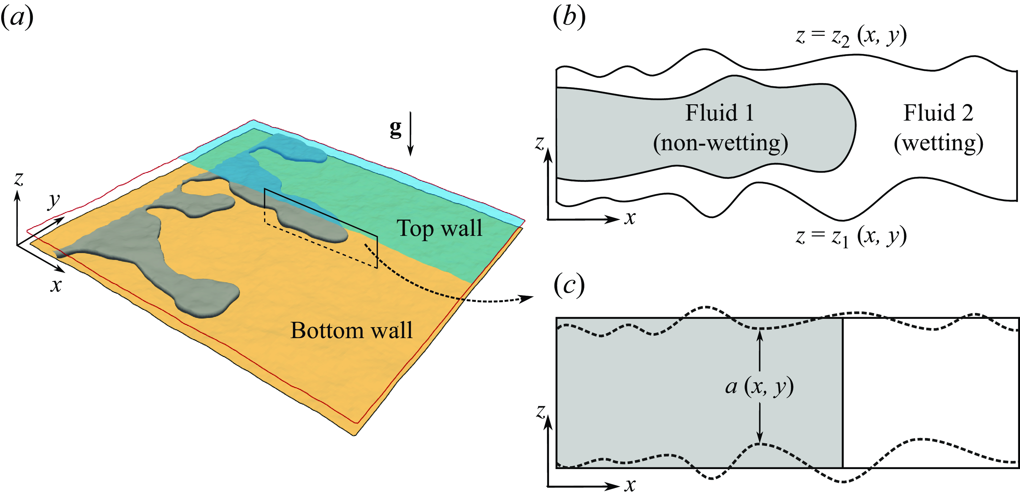
Figure 1. $(a)$
Three-dimensional (3-D) illustration of immiscible two-phase flow in a rough fracture of mean horizontal plane (
$(a)$
Three-dimensional (3-D) illustration of immiscible two-phase flow in a rough fracture of mean horizontal plane ( $xy$
). (b) Vertical (
$xy$
). (b) Vertical ( $xz$
) cross-sectional view of the 3-D displacement: the non-wetting fluid 1 (darker region) displaces the wetting fluid 2, leading to the formation of a wetting film adhering to the top and bottom walls.
$xz$
) cross-sectional view of the 3-D displacement: the non-wetting fluid 1 (darker region) displaces the wetting fluid 2, leading to the formation of a wetting film adhering to the top and bottom walls. $(c)$
The 2-D depth-integrated formulation reduces the description to two dimensions in the
$(c)$
The 2-D depth-integrated formulation reduces the description to two dimensions in the $xy$
plane, and can thus not account for the presence of such a wetting film; this is equivalent to assuming a fluid–fluid interface that does not depend on the vertical coordinate
$xy$
plane, and can thus not account for the presence of such a wetting film; this is equivalent to assuming a fluid–fluid interface that does not depend on the vertical coordinate $z$
in three dimensions. The thickness in the vertical direction is only shown for illustration, as it has no physical meaning in the 2-D formulation.
$z$
in three dimensions. The thickness in the vertical direction is only shown for illustration, as it has no physical meaning in the 2-D formulation.
We define the 2-D depth-averaged velocity field $\boldsymbol{U} = (U,V)$
as
$\boldsymbol{U} = (U,V)$
as
 \begin{equation} U (x,y)= \frac {1}{a(x,y)}\int _{z_1(x,y)}^{z_2(x,y)} u\:\text{d}z\quad \text{ and }\quad V(x,y) = \frac {1}{a(x,y)}\int _{z_1(x,y)}^{z_2(x,y)} v\:\text{d}z. \end{equation}
In the framework of the VOF formulation of two-phase flow, the definition of the bulk phase velocity also applies to the 2-D velocity field, i.e.
 \begin{equation} \boldsymbol{U} = \gamma \boldsymbol{U}_1 + (1-\gamma)\boldsymbol{U}_2. \end{equation}
3.2. Depth-integrated formalism for single-phase flow
For single-phase, incompressible flow, where a single fluid occupies the entire flow domain, the governing flow equations are the continuity and momentum conservation, which read respectively as
 \begin{equation} \boldsymbol{\nabla } \cdot \boldsymbol{u} = 0,\end{equation}
 \begin{equation} \text{and }\frac {\partial \left ( \rho \boldsymbol{u}\right)}{\partial t} + \left [ \boldsymbol{u} \cdot \left ( \rho \boldsymbol{\nabla } \right)\right] \boldsymbol{u} = -\boldsymbol{\nabla } p_{{d}} + \boldsymbol{\nabla }\cdot \left [ \mu \boldsymbol{\nabla } \boldsymbol{u} \right]. \end{equation}
Below, we integrate these governing 3-D equations over the $z$
coordinate, and the resulting integrals are then simplified using the Leibniz theorem and the fundamental theorem of calculus, along with the no-slip boundary condition for the velocity at the walls, to obtain the 2-D equations for the equivalent depth-integrated model.
$z$
coordinate, and the resulting integrals are then simplified using the Leibniz theorem and the fundamental theorem of calculus, along with the no-slip boundary condition for the velocity at the walls, to obtain the 2-D equations for the equivalent depth-integrated model.
3.2.1. Depth-integrated continuity equation
Integrating the continuity equation, (3.3), over $z$
, yields
$z$
, yields
 \begin{equation} \int _{z_1}^{z_2}\boldsymbol{\nabla } \cdot \boldsymbol{u} \text{d}z = \frac {\partial (a U)}{\partial x} + \frac {\partial (a V)}{\partial y} = \boldsymbol{\nabla }\cdot \left ( a\boldsymbol{U} \right) = 0, \end{equation}
where we have used the definitions of the 2-D velocity field from (3.1). The above equation indicates that, unlike in the 3-D model where the velocity field $\boldsymbol{u}$
is divergence free, in the 2-D depth-integrated model the divergence-free constraint applies to the quantity
$\boldsymbol{u}$
is divergence free, in the 2-D depth-integrated model the divergence-free constraint applies to the quantity
 \begin{equation} \boldsymbol{Q} = a\boldsymbol{U}, \end{equation}
which has been previously termed local flux in the literature (Méheust & Schmittbuhl Reference Méheust and Schmittbuhl2001).
3.2.2. Depth-integrated momentum equation
Next, we perform the depth-integration of the momentum equation (3.4), and develop the terms one by one as follows.
Temporal derivative of the momentum density
 \begin{equation} \int _{z_1}^{z_2}\frac {\partial \rho \boldsymbol{u}}{\partial t} \text{d}z = \frac {\partial \left (\rho a\boldsymbol{U}\right)}{\partial t} = \frac {\partial \left (\rho \boldsymbol{Q}\right)}{\partial t}. \end{equation}
3.2.2.1. Convective derivative of the momentum density:
Depth integration of the inertial term, when written in component form, e.g. for the $x$
direction, and considering the no-slip conditions on the top and bottom walls, reads as
$x$
direction, and considering the no-slip conditions on the top and bottom walls, reads as
 \begin{equation} \int _{z_1}^{z_2}\frac {\partial (\rho uu)}{\partial x}\:\text{d}z + \int _{z_1}^{z_2}\frac {\partial (\rho uv)}{\partial y} \:\text{d}z = \frac {\partial }{\partial x}\int _{z_1}^{z_2}\rho (uu)\:\text{d}z + \frac {\partial }{\partial y}\int _{z_1}^{z_2} \rho (uv)\:\text{d}z. \end{equation}
The integration of the $y$
component can be treated in the same way. We notice in the above equation the appearance of the nonlinear terms,
$y$
component can be treated in the same way. We notice in the above equation the appearance of the nonlinear terms, $\int _{z_1}^{z_2}\rho u_iu_j\: \text{d}z$
, where
$\int _{z_1}^{z_2}\rho u_iu_j\: \text{d}z$
, where $i,j\in 1,2$
are the indices denoting the
$i,j\in 1,2$
are the indices denoting the $u, v$
velocity components. There is no general integrated form for these integrals, as they depend on the vertical velocity profile. They can be expressed by using a momentum correction factor
$u, v$
velocity components. There is no general integrated form for these integrals, as they depend on the vertical velocity profile. They can be expressed by using a momentum correction factor $\beta$
which accounts for the
$\beta$
which accounts for the $z$
-dependence of the velocity field (Chanson Reference Chanson2004)
$z$
-dependence of the velocity field (Chanson Reference Chanson2004)
 \begin{equation} \int _{z_1}^{z_2}\rho (u_{i} u_{j})\: \text{d}z = \beta \:\rho \: (U_i U_{j})\:a\:. \end{equation}
The depth-integrated inertial term in vectorial form can thus be written as
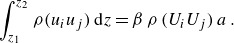
 \begin{equation} \int _{z_1}^{z_2}\left [ \boldsymbol{u} \cdot \left ( \rho \boldsymbol{\nabla } \right) \right] \boldsymbol{u} \: \text{d}z = \beta \:\left [\boldsymbol{U} \cdot \left ( \rho \boldsymbol{\nabla } \right) \right] \boldsymbol{U}a. \end{equation}
The approximation made above is reasonable on account of our lubrication assumption $\mathcal{A}$
(i), which implies a parabolic vertical velocity profile. Consequently, we use
$\mathcal{A}$
(i), which implies a parabolic vertical velocity profile. Consequently, we use $\beta =1.2$
in this study, corresponding to a parabolic vertical velocity profile throughout the fracture plane (similar to that observed in plane Poiseuille flow (Gerhart, Hochstein & Gerhart Reference Gerhart, Hochstein and Gerhart2020)).
$\beta =1.2$
in this study, corresponding to a parabolic vertical velocity profile throughout the fracture plane (similar to that observed in plane Poiseuille flow (Gerhart, Hochstein & Gerhart Reference Gerhart, Hochstein and Gerhart2020)).
3.2.2.2. Dynamic pressure force:
Using assumption $\mathcal{A}$
(ii) of constant pressure in the
$\mathcal{A}$
(ii) of constant pressure in the $z$
direction, depth integrating the pressure term results in the following:
$z$
direction, depth integrating the pressure term results in the following:
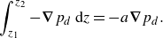 \begin{equation} \int _{z_1}^{z_2}-\boldsymbol{\nabla } p_{{d}} \: \text{d}z = - a\boldsymbol{\nabla } p_{{d}}. \end{equation}
3.2.2.3. Viscous force:
Depth integrating the last term of the momentum equation (3.4), which accounts for the viscous dissipation, we obtain, for the component form in $x$
$x$
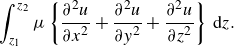 \begin{equation} \int _{z_1}^{z_2}\mu \left \lbrace \frac {\partial ^2u}{\partial x^2}+\frac {\partial ^2u}{\partial y^2}+\frac {\partial ^2u}{\partial z^2}\right \rbrace \: \text{d}z. \end{equation}
Applying the Leibniz rule twice to $\partial ^2 ( \int _{z_1}^{z_2} u \text{d}z) / \partial x^2$
, considering the no-flow boundary conditions at the walls and using the depth-averaged field definition (3.1), leads to
$\partial ^2 ( \int _{z_1}^{z_2} u \text{d}z) / \partial x^2$
, considering the no-flow boundary conditions at the walls and using the depth-averaged field definition (3.1), leads to
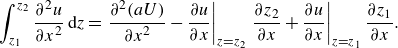 \begin{equation} \int _{z_1}^{z_2}\frac {\partial ^2u}{\partial x^2}\: \text{d}z = \left.\frac {\partial ^2(aU)}{\partial x^2} - \frac {\partial u}{\partial x}\right |_{z=z_2} \left.\frac {\partial z_2}{\partial x} +\frac {\partial u}{\partial x}\right |_{z=z_1} \frac {\partial z_1}{\partial x}. \end{equation}
In the case of a flat surface (e.g. Hele-Shaw cell), the last two terms on the right-hand side of the above equation vanish. For surfaces with spatially varying apertures, they are not expected to entirely vanish, but, based on the lubrication approximation $\mathcal{A}$
(i), they can be neglected. A similar simplification can be made for the second integral of (3.12), leaving the last term, which results in
$\mathcal{A}$
(i), they can be neglected. A similar simplification can be made for the second integral of (3.12), leaving the last term, which results in
 \begin{equation} \int _{z_1}^{z_2}\mu \frac {\partial ^2u}{\partial z^2}\: \text{d}z\: =\: \mu \left.\frac {\partial u}{\partial z}\right |_{z=z_2} -\:\: \mu \left.\frac {\partial u}{\partial z}\right |_{z=z_1}. \end{equation}
This is the $x$
component
$x$
component $\tau _{w,x}$
of the wall shear stress resulting from the no-slip boundary conditions at the fracture walls. Hence, (3.12) can be written as
$\tau _{w,x}$
of the wall shear stress resulting from the no-slip boundary conditions at the fracture walls. Hence, (3.12) can be written as
 \begin{equation} \mu \left \lbrace \frac {\partial ^2(aU)}{\partial x^2}+\frac {\partial ^2(aU)}{\partial y^2}\right \rbrace + \tau _{w,x}. \end{equation}
The procedure outlined above can then be repeated for the $y$
component of the viscous term, where the component of the wall shear stress becomes
$y$
component of the viscous term, where the component of the wall shear stress becomes $\tau _{w,y}$
. In vectorial notation, the depth-integrated viscous term can finally be written as
$\tau _{w,y}$
. In vectorial notation, the depth-integrated viscous term can finally be written as
 \begin{equation} \int _{z_1}^{z_2}\boldsymbol{\nabla }\cdot (\mu \boldsymbol{\nabla }\boldsymbol{u})\: \text{d}z = \boldsymbol{\nabla }\cdot \left [ \mu \boldsymbol{\nabla } (a\boldsymbol{U}) \right]+ \boldsymbol{\tau _{w}} = \boldsymbol{\nabla }\cdot \left (\mu \boldsymbol{\nabla } \boldsymbol Q \right) + \boldsymbol{\tau _{w}}, \end{equation}
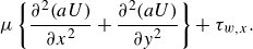
where, $\boldsymbol{\tau _{w}}$
is the wall shear stress vector accounting for the drag by the fracture walls. There is no general theoretical expression for this drag term as it depends on the
$\boldsymbol{\tau _{w}}$
is the wall shear stress vector accounting for the drag by the fracture walls. There is no general theoretical expression for this drag term as it depends on the $z$
-dependence of the velocity. However, as mentioned above, with the assumption of a parabolic vertical velocity profile, the drag term can then be calculated to be the following Darcian term:
$z$
-dependence of the velocity. However, as mentioned above, with the assumption of a parabolic vertical velocity profile, the drag term can then be calculated to be the following Darcian term:
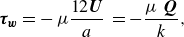 \begin{equation} \boldsymbol{\tau _{w}} = -\:\mu \frac {12 \boldsymbol{U}}{a}\: = -\frac {\mu \: \boldsymbol{Q}}{k}, \end{equation}
where $k=a^2/12$
is the local parallel plate permeability of the fracture.
$k=a^2/12$
is the local parallel plate permeability of the fracture.
3.2.3. Complete depth-integrated model for monophasic flow
Putting together the integrals of the individual terms discussed above, the 2-D depth-integrated single-phase flow equations can now be expressed as a function of the local flux $\boldsymbol Q$
(defined in (3.6)) as follows:
$\boldsymbol Q$
(defined in (3.6)) as follows:
 \begin{equation} \boldsymbol{\nabla }\cdot \boldsymbol{Q} = 0, \end{equation}
 \begin{equation} \frac {\partial (\rho \boldsymbol{Q})}{\partial t} + \beta \left [ \frac {\boldsymbol{Q}}{a} \cdot \left ( \rho \boldsymbol{\nabla } \right) \right] \boldsymbol Q = \:-a\boldsymbol{\nabla } p_{{d}} + \boldsymbol{\nabla }\cdot \left (\mu \boldsymbol{\nabla } \boldsymbol Q \right) -\frac {12 \mu }{a^2} \boldsymbol{Q}. \end{equation}
Note that the conserved quantity in this 2-D model is the local flux $\boldsymbol Q$
. The 2-D depth-averaged velocity
$\boldsymbol Q$
. The 2-D depth-averaged velocity $\boldsymbol{U} = \boldsymbol{Q}/a$
is obtained as a post-processed quantity. The particular case of steady-state Stokes flow yields the well-known Reynolds equation (Brown Reference Brown1987), as discussed in Appendix A.
$\boldsymbol{U} = \boldsymbol{Q}/a$
is obtained as a post-processed quantity. The particular case of steady-state Stokes flow yields the well-known Reynolds equation (Brown Reference Brown1987), as discussed in Appendix A.
3.3. Depth-integrated formalism for two-phase flow
We now combine the VOF formulation for two-phase flow, as outlined in § 2, and the depth-integrated approach presented in § 3.2, based on the same assumptions.
3.3.1. Depth-integrated continuity equation
As for the monophasic case, depth-integrating the two-phase continuity equation (2.1) leads to
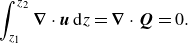 \begin{equation} \int _{z_1}^{z_2}\boldsymbol{\nabla } \cdot \boldsymbol{u} \: \text{d}z = \boldsymbol{\nabla }\cdot \boldsymbol{Q} = 0. \end{equation}
3.3.2. Depth-integrated phase-fraction advection equation
Using the assumption $\mathcal{B}$
made in § 3.1, i.e. neglecting the presence of displaced fluid films on the fracture walls, amounts to assuming that the indicator function
$\mathcal{B}$
made in § 3.1, i.e. neglecting the presence of displaced fluid films on the fracture walls, amounts to assuming that the indicator function $\gamma$
does not depend on
$\gamma$
does not depend on $z$
. Hence, depth integrating the phase-fraction advection equation (2.9), first without taking into account the ‘compression term’, yields
$z$
. Hence, depth integrating the phase-fraction advection equation (2.9), first without taking into account the ‘compression term’, yields
 \begin{equation} a\:\frac {\partial \gamma }{\partial t} + \boldsymbol{Q} \cdot \boldsymbol{\nabla } \gamma = 0. \end{equation}
To reduce numerical diffusion, we then introduce an additional compression term $\boldsymbol{\nabla }\cdot [\boldsymbol{Q}_{{r}}\gamma (1-\gamma)]$
, analogous to the compression term introduced in (2.9). In this 2-D formulation of the compression term, the compression local flux
$\boldsymbol{\nabla }\cdot [\boldsymbol{Q}_{{r}}\gamma (1-\gamma)]$
, analogous to the compression term introduced in (2.9). In this 2-D formulation of the compression term, the compression local flux $\boldsymbol{Q}_{{r}}$
is analogous to the compression velocity
$\boldsymbol{Q}_{{r}}$
is analogous to the compression velocity $\boldsymbol u_{{r}}$
in (2.10), and is similarly defined, as
$\boldsymbol u_{{r}}$
in (2.10), and is similarly defined, as
 \begin{equation} \boldsymbol{Q}_{{r}} = \textrm{min}\:[C_{\gamma }\:\|\boldsymbol{Q}\|,\:\: \textrm{max}\:(\|\boldsymbol{Q}\|)]\:\boldsymbol{n}. \end{equation}
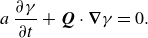
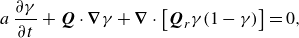
The complete depth-integrated phase-fraction equation is thus given by
 \begin{equation} a\:\frac {\partial \gamma }{\partial t} + \boldsymbol{Q} \cdot \boldsymbol{\nabla } \gamma + \boldsymbol{\nabla }\cdot \left [\boldsymbol{Q}_{{r}}\gamma (1-\gamma)\right] = 0. \end{equation}
Note that, in the above equation, the aperture field $a(x,y)$
modifies the temporal derivative of the phase-fraction
$a(x,y)$
modifies the temporal derivative of the phase-fraction $\gamma$
, and thus accounts for the storage capacity available at any location.
$\gamma$
, and thus accounts for the storage capacity available at any location.
3.3.3. Depth-integrated momentum equation
We now perform the depth-integration of the two-phase momentum equation in its final form (2.13). The integrals for the temporal and the convective derivatives of the momentum density, as well as the dynamic pressure force, read identically to the corresponding monophasic integrals (see § 3.2.2, (3.7), (3.10) and (3.11) respectively). The remaining integrals are presented as follows.
3.3.3.1. Viscous force
Compared with the single-phase case, the viscous dissipation term(s) in the two-phase momentum equation (2.13) has an additional contribution arising from the viscosity gradient, which is non-negligible in the interface region. The depth integration of these two terms reads as
 \begin{equation} \int _{z_1}^{z_2} \boldsymbol{\nabla }\cdot \left (\mu \boldsymbol{\nabla }\boldsymbol{u}\right) \text{d}z + \int _{z_1}^{z_2} \boldsymbol{\nabla }\boldsymbol{u} \cdot \nabla \mu \: \text{d}z. \end{equation}
Using assumption $\mathcal{B}$
(§ 3.1), the derivative of the viscosity with respect to
$\mathcal{B}$
(§ 3.1), the derivative of the viscosity with respect to $z$
can be neglected. Hence, integrating the first term leads to the same formulation as for the single-phase viscous term integral (3.16). When written in component form, the integral of the
$z$
can be neglected. Hence, integrating the first term leads to the same formulation as for the single-phase viscous term integral (3.16). When written in component form, the integral of the $x$
component of the second term can be written as
$x$
component of the second term can be written as
 \begin{equation} \int _{z_1}^{z_2} \left \lbrace \frac {\partial u}{\partial x} \frac {\partial \mu }{\partial x} + \frac {\partial u}{\partial y} \frac {\partial \mu }{\partial y} + \frac {\partial u}{\partial z} \frac {\partial \mu }{\partial z} \right \rbrace \:\text{d}z\:, \end{equation}
where the last term can be neglected ( $\partial \mu / \partial z \simeq 0$
). Again, as a consequence of the lubrication approximation, we can assume that the in-plane gradient of viscosity is independent of
$\partial \mu / \partial z \simeq 0$
). Again, as a consequence of the lubrication approximation, we can assume that the in-plane gradient of viscosity is independent of $z$
; using the 2-D averaged velocity definition (3.1), the integrals can then be simplified to
$z$
; using the 2-D averaged velocity definition (3.1), the integrals can then be simplified to
 \begin{equation} \int _{z_1}^{z_2} \left \lbrace \frac {\partial u}{\partial x} \frac {\partial \mu }{\partial x} + \frac {\partial u}{\partial y} \frac {\partial \mu }{\partial y} \right \rbrace \:\text{d}z\:=\:\frac {\partial \mu }{\partial x} \frac {\partial (aU)}{\partial x} + \frac {\partial \mu }{\partial y} \frac {\partial (aU)}{\partial y} \:. \end{equation}
A similar argument can be used to simplify the $y$
component of the integral of
$y$
component of the integral of $\boldsymbol{\nabla }\boldsymbol{u} \cdot \nabla \mu$
, and finally, we obtain the following expression for the depth-integrated viscous force:
$\boldsymbol{\nabla }\boldsymbol{u} \cdot \nabla \mu$
, and finally, we obtain the following expression for the depth-integrated viscous force:
 \begin{equation} \int _{z_1}^{z_2}\boldsymbol{\nabla }\cdot \left (\mu \boldsymbol{\nabla }\boldsymbol{u}\right)\: \text{d}z + \int _{z_1}^{z_2}\boldsymbol{\nabla }\boldsymbol{u} \cdot \nabla \mu \: \text{d}z = \boldsymbol{\nabla }\cdot \left (\mu \boldsymbol{\nabla }\boldsymbol{Q}\right) + \boldsymbol{\nabla }\boldsymbol{Q}\cdot \nabla \mu -\frac {12 \mu }{a^2} \boldsymbol{Q} \:. \end{equation}
3.3.3.2. Density gradient term
The depth integration of the term containing gravity and the density gradient (which is significant only at the interface) results in
 \begin{equation} \begin{aligned} \int _{z_1}^{z_2}\left ( \boldsymbol{g}\cdot \boldsymbol{x} \right) \boldsymbol{\nabla }\rho \: \text{d}z = \boldsymbol{\nabla }\rho \int _{z_1}^{z_2}\left (g_xx+g_yy+g_zz\right)\text{d}z = \left (a\boldsymbol g_{ \|}\cdot \boldsymbol{x}\:+ a g_z \frac {(z_1 + z_2)}{2} \right) \boldsymbol{\nabla }\rho, \end{aligned} \end{equation}
where $\boldsymbol{g}_\| = (g_x,g_y)$
is the projection of the gravity acceleration onto the mean fracture plane, and
$\boldsymbol{g}_\| = (g_x,g_y)$
is the projection of the gravity acceleration onto the mean fracture plane, and $g_z$
is its component in the direction normal to that plane (
$g_z$
is its component in the direction normal to that plane ( $z$
direction). The above integral shows that for the 2-D integrated model, to fully describe the gravitational effects, an additional geometric field, namely the mean vertical positions of the fracture, is needed. It must be noted that in the right-hand side of the above equation, the position vector
$z$
direction). The above integral shows that for the 2-D integrated model, to fully describe the gravitational effects, an additional geometric field, namely the mean vertical positions of the fracture, is needed. It must be noted that in the right-hand side of the above equation, the position vector $\boldsymbol{x}$
is restricted to two dimensions
$\boldsymbol{x}$
is restricted to two dimensions $x$
and
$x$
and $y$
.
$y$
.
3.3.3.3. Surface tension force
The curvature $\kappa$
, which is defined by (2.7), is the sum of the in-plane curvature
$\kappa$
, which is defined by (2.7), is the sum of the in-plane curvature $\kappa _{xy}$
and the out-of-plane curvature
$\kappa _{xy}$
and the out-of-plane curvature $\kappa _{z}$
. For the 2-D depth-integrated model, where no out-of-plane curvature can be described by the model, the corresponding capillary force contribution must be taken into account explicitly by adding to
$\kappa _{z}$
. For the 2-D depth-integrated model, where no out-of-plane curvature can be described by the model, the corresponding capillary force contribution must be taken into account explicitly by adding to $\kappa$
a term that accounts for the out-of-plane curvature
$\kappa$
a term that accounts for the out-of-plane curvature
 \begin{equation} \kappa = -\boldsymbol{\nabla }\cdot \left (\frac {\boldsymbol{\nabla }\gamma }{\|\boldsymbol{\nabla }\gamma \|}\right) - \frac {2}{a}\:\cos \:\theta _{{e}} \:, \end{equation}
where $\theta _{{e}}$
is an effective contact angle at fluid–fluid–solid contact lines. This angle is not necessarily the real equilibrium contact angle; its value is discussed at the beginning of § 4.
$\theta _{{e}}$
is an effective contact angle at fluid–fluid–solid contact lines. This angle is not necessarily the real equilibrium contact angle; its value is discussed at the beginning of § 4.
Here, we have used our assumption $\mathcal{A}$
of small gradients for the aperture field and assumed for the out-of-plane term that the vertical velocity profiles are parabolic everywhere in the fracture plane (which is also classically assumed to derive the local cubic law for stationary monophasic flow) (Park & Homsy Reference Park and Homsy1984). The above approximation of the out-of-plane curvature term may be oversimplifying in cases where deviations from a symmetric interface are to be expected, such as surfaces with different wetting properties on opposite sides, such as may occur in configurations of heterogeneous wetting properties of the fracture walls. With this assumption, the depth-integrated surface tension is then evaluated as
$\mathcal{A}$
of small gradients for the aperture field and assumed for the out-of-plane term that the vertical velocity profiles are parabolic everywhere in the fracture plane (which is also classically assumed to derive the local cubic law for stationary monophasic flow) (Park & Homsy Reference Park and Homsy1984). The above approximation of the out-of-plane curvature term may be oversimplifying in cases where deviations from a symmetric interface are to be expected, such as surfaces with different wetting properties on opposite sides, such as may occur in configurations of heterogeneous wetting properties of the fracture walls. With this assumption, the depth-integrated surface tension is then evaluated as
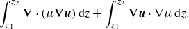
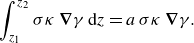 \begin{equation} \int _{z_1}^{z_2}\sigma \kappa \:\boldsymbol{\nabla }\gamma \:\text{d}z = a\:\sigma \kappa \:\boldsymbol{\nabla }\gamma. \end{equation}
3.3.4. Complete theoretical description for two-phase flow
Finally, we can now write the two-phase 2-D depth-integrated governing equations as
 \begin{equation} \boldsymbol{\nabla } \cdot \boldsymbol{Q} = 0,\end{equation}
 \begin{equation} a\:\frac {\partial \gamma }{\partial t} + \boldsymbol{Q} \cdot \boldsymbol{\nabla } \gamma + \boldsymbol{\nabla }\cdot \left [\boldsymbol{Q}_r\gamma (1-\gamma)\right] = 0,\end{equation}
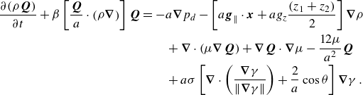 \begin{equation} \begin{aligned} \frac {\partial (\rho \boldsymbol{Q})}{\partial t} + \beta \left [ \frac {\boldsymbol{Q}}{a} \cdot \left ( \rho \boldsymbol{\nabla } \right) \right] \boldsymbol{Q} &= -a\boldsymbol{\nabla } p_{{d}} - \left [ a\boldsymbol{g}_{\|} \cdot \boldsymbol{x} + a g_z \frac {(z_1 + z_2)}{2} \right] \boldsymbol{\nabla } \rho \\ &\qquad +\boldsymbol{\nabla } \cdot \left ( \mu \boldsymbol{\nabla } \boldsymbol{Q} \right) + \boldsymbol{\nabla } \boldsymbol{Q} \cdot \boldsymbol{\nabla } \mu - \frac {12 \mu }{a^2} \boldsymbol{Q} \\ &\qquad + a\sigma \left [ \boldsymbol{\nabla } \cdot \left ( \frac {\boldsymbol{\nabla } \gamma }{\| \boldsymbol{\nabla } \gamma \|} \right) + \frac {2}{a} \cos \theta \right] \boldsymbol{\nabla } \gamma \:. \end{aligned} \end{equation}
3.4. Solution procedure with OpenFOAM
All numerical simulations have been implemented using the open-source CFD code OpenFOAM (2012), which employs a cell-centre-based finite volume approach for spatial discretisation with second-order accuracy. For time integration, the implicit Euler scheme is used, which results in first-order accuracy in time. The computational mesh for both the 3-D and 2-D models was generated using the blockMesh utility of OpenFOAM, which results in structured hexahedral elements. Although all our simulations use structured hexahedral mesh elements, the 2-D depth-integrated model implementation is not restricted to such mesh elements, and can easily be applied to other mesh alternatives, e.g. unstructured tetrahedral cells.
The monophasic 3-D governing equations ((3.3) and (3.4)) are solved using pisoFoam, which is a transient, single-phase, Navier–Stokes solver provided in OpenFOAM. We employ the interFoam solver of OpenFOAM to solve the two-phase governing equations for the 3-D VOF model ((2.1), (2.9) and (2.13)). The numerical implementation of the 2-D depth-integrated models, both single phase ((3.18) and (3.19)) and two phase ((3.31), (3.32) and (3.33)), is performed by modifying the two aforementioned solvers in OpenFOAM. While the overall solution algorithm remains largely the same, our changes to the solvers account for the change of variable from the 3-D velocity field $\boldsymbol u$
to the 2-D local flux
$\boldsymbol u$
to the 2-D local flux $\boldsymbol Q$
, and for the additional terms appearing in the governing equations, e.g. the Darcian drag term in the momentum equation. For details on the finite volume discretisation methods and the solution procedures of the two Navier–Stokes solvers namely, pisoFoam and interFoam, the reader is encouraged to see Jasak (Reference Jasak1996), Weller et al. (Reference Weller, Tabor, Jasak and Fureby1998), Rusche (Reference Rusche2003), Berberović et al. (Reference Berberović, van Hinsberg, Jakirlić, Roisman and Tropea2009) and Deshpande et al. (Reference Deshpande, Anumolu and Trujillo2012a
). In all simulations, we initialise the time step with a very low value (
$\boldsymbol Q$
, and for the additional terms appearing in the governing equations, e.g. the Darcian drag term in the momentum equation. For details on the finite volume discretisation methods and the solution procedures of the two Navier–Stokes solvers namely, pisoFoam and interFoam, the reader is encouraged to see Jasak (Reference Jasak1996), Weller et al. (Reference Weller, Tabor, Jasak and Fureby1998), Rusche (Reference Rusche2003), Berberović et al. (Reference Berberović, van Hinsberg, Jakirlić, Roisman and Tropea2009) and Deshpande et al. (Reference Deshpande, Anumolu and Trujillo2012a
). In all simulations, we initialise the time step with a very low value ( ${\sim}10^{-8}$
s) and employ a run-time adjustable time-step scheme, which ensures numerical stability by automatically adjusting the time steps according to the Courant–Friedrichs–Lewy (CFL) criterion (Rusche Reference Rusche2003). The maximum allowed CFL number for all cases is set to
${\sim}10^{-8}$
s) and employ a run-time adjustable time-step scheme, which ensures numerical stability by automatically adjusting the time steps according to the Courant–Friedrichs–Lewy (CFL) criterion (Rusche Reference Rusche2003). The maximum allowed CFL number for all cases is set to $0.5$
.
$0.5$
.
4. Results and discussions
In this section, we begin by validating the two-phase, 2-D depth-integrated model through comparison with results from corresponding 3-D direct numerical simulations for the classic Hele-Shaw viscous fingering case, following the study by Saffman & Taylor (Reference Saffman and Taylor1958). It must be noted, that the validation of the 3-D model has been discussed in detail in our previous work (Krishna et al. Reference Krishna, Méheust and Neuweiler2024), thus interested readers may refer to it. Subsequently, we apply the 2-D model to a synthetic rough fracture geometry, comparing its performance against the 3-D model results. As an initial step in validating the 2-D model, we have also compared the single-phase 2-D results with those from the full 3-D model for the fracture geometry. These comparisons are detailed in Appendix E.
4.1. Choice of the effective contact angle in the depth-integrated model
The theoretical description of the out-of-plane curvature contribution presented above in § 3.2.2, (3.29) assumes the absence of a wetting film. However, as a wetting film is expected and was also found in all 3-D film-resolved simulations, using the static equilibrium contact angle as effective contact angle in (3.29) of the 2-D depth-integrated model is not consistent with the physics at play. This effect is also illustrated in figure 20 in Appendix B for the idealised case of the flow between two smooth parallel plates (Hele-Shaw cell configuration). The presence of a thin wetting film of the defending fluid on the top and bottom walls increases the curvature of the interface at the finger tip, as compared with a scenario where no wetting film would be present. Assuming the tip to be circular (which is reasonable since local apertures are small and much smaller than the in-plane radius of curvature of the interface), and depending on the film thickness, the effective meniscus, estimated as the circle tangent to the finger at its tip, may either not meet the cell walls (in most cases, in which case the best estimate for the effective contact angle is $\theta _{{e}}=180^\circ$
) or meet them at an angle different from that of the equilibrium contact angle
$\theta _{{e}}=180^\circ$
) or meet them at an angle different from that of the equilibrium contact angle $\theta$
. By considering the angle at which the circle meets the walls as an effective contact angle, the out-of-plane curvature estimate (3.29) could be improved by accounting for the film thickness (Park & Homsy Reference Park and Homsy1984) and its dependence on the capillary number (see Appendix C). As this approach would imply using a local capillary number (Anjos et al. Reference Anjos, Zhao, Lowengrub, Bao and Li2021) and as the derivations are based on flat surfaces, so the validity for rough surfaces is a priori unclear. This effect is not accounted for in the model.
$\theta$
. By considering the angle at which the circle meets the walls as an effective contact angle, the out-of-plane curvature estimate (3.29) could be improved by accounting for the film thickness (Park & Homsy Reference Park and Homsy1984) and its dependence on the capillary number (see Appendix C). As this approach would imply using a local capillary number (Anjos et al. Reference Anjos, Zhao, Lowengrub, Bao and Li2021) and as the derivations are based on flat surfaces, so the validity for rough surfaces is a priori unclear. This effect is not accounted for in the model.
In this work, to ensure consistency between the 2-D and 3-D models, we adopt an effective contact angle value of $\theta _{{e}}=180^\circ$
for approximating the out-of-plane curvature and the resulting capillary pressure component. Supporting analysis of the finger tip curvature and the effective contact angle in the resolved-film Hele-Shaw configuration is presented in Appendix B. Furthermore, the sensitivity of our 2-D model to variations in contact angle is discussed in Appendix C.
$\theta _{{e}}=180^\circ$
for approximating the out-of-plane curvature and the resulting capillary pressure component. Supporting analysis of the finger tip curvature and the effective contact angle in the resolved-film Hele-Shaw configuration is presented in Appendix B. Furthermore, the sensitivity of our 2-D model to variations in contact angle is discussed in Appendix C.
4.2. Validation of the two-phase 2-D depth-integrated model
We validate our two-phase 2-D depth-integrated model by examining viscous fingering in a conventional Hele-Shaw cell, which consists of two parallel planar walls separated by a fixed aperture $a(x,y) = b$
that is much smaller than the wall’s extension along their plane (figure 2). This set-up replicates the classic experiment by Saffman & Taylor (Reference Saffman and Taylor1958), where a less viscous fluid displaces a more viscous one, leading to the formation of a stable finger with a width-to-channel width ratio (
$a(x,y) = b$
that is much smaller than the wall’s extension along their plane (figure 2). This set-up replicates the classic experiment by Saffman & Taylor (Reference Saffman and Taylor1958), where a less viscous fluid displaces a more viscous one, leading to the formation of a stable finger with a width-to-channel width ratio ( $\lambda$
) of 0.5, except at very slow driving velocities, for which
$\lambda$
) of 0.5, except at very slow driving velocities, for which $\lambda$
approaches 1.0.
$\lambda$
approaches 1.0.
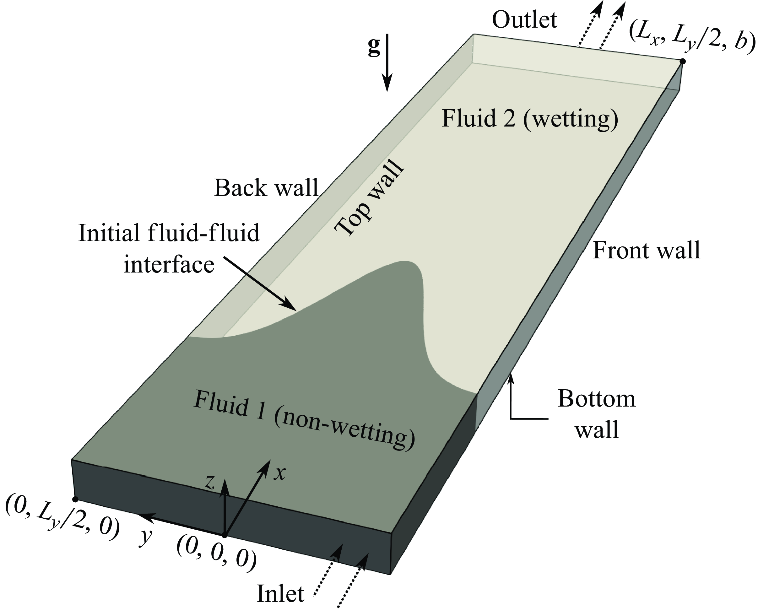
Figure 2. Schematic of the Hele-Shaw cell used for validating the 2-D depth-integrated two-phase flow model against the 3-D model. The cell dimensions are: length $L_x=100$
mm (
$L_x=100$
mm ( $x\in [0,L_x]$
), width
$x\in [0,L_x]$
), width $L_y=12.5$
mm (
$L_y=12.5$
mm ( $y\in [-L_y/2,L_y/2]$
) and constant vertical aperture
$y\in [-L_y/2,L_y/2]$
) and constant vertical aperture $b=0.4$
mm (
$b=0.4$
mm ( $z\in [0,b]$
). The width-to-thickness ratio is
$z\in [0,b]$
). The width-to-thickness ratio is $L_y/b = 31.25$
. The initial fluid–fluid interface (at
$L_y/b = 31.25$
. The initial fluid–fluid interface (at $t=0$
) has Gaussian profile in the horizontal (
$t=0$
) has Gaussian profile in the horizontal ( $xy$
) plane. The darker region represents the invading fluid and the lighter region the defending fluid.
$xy$
) plane. The darker region represents the invading fluid and the lighter region the defending fluid.
4.2.1. Numerical set-up and flow conditions
The numerical set-up for validation (shown in figure 2) is adapted from the original configuration by Saffman & Taylor (Reference Saffman and Taylor1958), with slight modifications to enhance computational efficiency. To promote a single dominant finger growth without extending the channel length excessively, we apply an initial perturbation to the fluid interface (figure 2). Fluid 1 represents the invading, less viscous, non-wetting phase, while fluid 2 is the defending, more viscous, wetting phase, with material properties listed in table 1. The viscosity ratio $\mu _2/\mu _1=30$
matches that of the original experiments. Flow conditions were defined by injection velocities
$\mu _2/\mu _1=30$
matches that of the original experiments. Flow conditions were defined by injection velocities $\boldsymbol{u}(x=0,y,z) = (u_{{in}},0,0)$
, where
$\boldsymbol{u}(x=0,y,z) = (u_{{in}},0,0)$
, where $u_{{in}}$
is the injection speed in the longitudinal
$u_{{in}}$
is the injection speed in the longitudinal $x$
direction. The resulting Reynolds (
$x$
direction. The resulting Reynolds ( $Re = \rho _1 u_{{in}} b / \mu _1$
) and capillary (
$Re = \rho _1 u_{{in}} b / \mu _1$
) and capillary ( $Ca = \mu _1 u_{{in}}/\sigma$
) numbers are provided in table 1. In the 2-D integrated model, where the primary variable is the local flux
$Ca = \mu _1 u_{{in}}/\sigma$
) numbers are provided in table 1. In the 2-D integrated model, where the primary variable is the local flux $\boldsymbol{Q} = (Q_x, Q_y)$
, the inlet flux is set to
$\boldsymbol{Q} = (Q_x, Q_y)$
, the inlet flux is set to $Q_{{in}}=u_{{in}}\:b$
.
$Q_{{in}}=u_{{in}}\:b$
.
Table 1. Fluid properties and flow parameters used for the Hele-Shaw channel simulations.
The 3-D computational mesh (figure 3
a) uses 40 cells in the $z$
direction, with finer grading near the walls to resolve the thin film. The 2-D mesh (figure 3
b) has a single cell in the
$z$
direction, with finer grading near the walls to resolve the thin film. The 2-D mesh (figure 3
b) has a single cell in the $z$
direction, without boundary conditions on the top and bottom faces. The boundary conditions imposed on different domain boundaries for both the 2-D and the 3-D models are listed in table 2.
$z$
direction, without boundary conditions on the top and bottom faces. The boundary conditions imposed on different domain boundaries for both the 2-D and the 3-D models are listed in table 2.
Figure 3. Computational mesh for the Hele-Shaw domain, featuring a horizontal discretisation of $\Delta x = b/8$
, where
$\Delta x = b/8$
, where $\Delta x = \Delta y$
is the characteristic uniform horizontal grid resolution in the
$\Delta x = \Delta y$
is the characteristic uniform horizontal grid resolution in the $xy$
plane. For the 3-D simulation (a), the cells near the top and bottom walls (
$xy$
plane. For the 3-D simulation (a), the cells near the top and bottom walls ( $z=0$
,
$z=0$
, $z=b$
) have a vertical resolution of
$z=b$
) have a vertical resolution of $0.3$
µm, while cells near the mid-plane (
$0.3$
µm, while cells near the mid-plane ( $z=b/2$
) have a resolution of
$z=b/2$
) have a resolution of $30$
µm. The cell-to-cell expansion ratio is 1.2, resulting in a total of
$30$
µm. The cell-to-cell expansion ratio is 1.2, resulting in a total of $2.0\times 10^7$
cells (
$2.0\times 10^7$
cells ( $250 \times 2000 \times 40$
). For the 2-D simulation (b), the vertical grid consists of one constant-size cell, with the total number of grid cells being
$250 \times 2000 \times 40$
). For the 2-D simulation (b), the vertical grid consists of one constant-size cell, with the total number of grid cells being $5.0\times 10^5$
(
$5.0\times 10^5$
( $250 \times 2000 \times 1$
).
$250 \times 2000 \times 1$
).
Table 2. Boundary conditions for the two-phase 3-D and 2-D depth-integrated numerical simulations. $\boldsymbol{n}_{{b}}$
denotes the normal to the boundaries other than the solid walls, namely the inlet and outlet.
$\boldsymbol{n}_{{b}}$
denotes the normal to the boundaries other than the solid walls, namely the inlet and outlet.
4.2.2. Validation and comparison with 3-D model results
We now compare the results obtained with the 2-D simulations based on the depth-averaged model with those obtained with the 3-D simulations.
Width and tip shape of the viscous finger: the evolution of the fluid–fluid interface for a representative case ( $Re=0.016$
,
$Re=0.016$
, $\log (Ca)=-3.18$
) is depicted in figure 4. Both the 3-D (figure 4
a) and 2-D (figure 4
b) simulations successfully reproduce the development of a single finger of the invading fluid, in line with the findings of Saffman & Taylor (Reference Saffman and Taylor1958). At
$\log (Ca)=-3.18$
) is depicted in figure 4. Both the 3-D (figure 4
a) and 2-D (figure 4
b) simulations successfully reproduce the development of a single finger of the invading fluid, in line with the findings of Saffman & Taylor (Reference Saffman and Taylor1958). At $x \approx 0.02$
m, in the neck region of the finger, its width in the 3-D case is notably larger than that observed in the 2-D simulation. This trend holds true across different injection velocities. Figure 4(c) shows the fluid–fluid interface in the longitudinal vertical mid-plane for the 3-D simulation at three different times. For the 2-D simulation, the interface is shown as the vertical line corresponding to the longitudinal mid-line at the same times. Note that, in agreement with previous studies (Bretherton Reference Bretherton1961; Horgue et al. Reference Horgue, Augier, Quintard and Prat2012), our 3-D simulations confirm that the thickness of the defending fluid film decreases as
$x \approx 0.02$
m, in the neck region of the finger, its width in the 3-D case is notably larger than that observed in the 2-D simulation. This trend holds true across different injection velocities. Figure 4(c) shows the fluid–fluid interface in the longitudinal vertical mid-plane for the 3-D simulation at three different times. For the 2-D simulation, the interface is shown as the vertical line corresponding to the longitudinal mid-line at the same times. Note that, in agreement with previous studies (Bretherton Reference Bretherton1961; Horgue et al. Reference Horgue, Augier, Quintard and Prat2012), our 3-D simulations confirm that the thickness of the defending fluid film decreases as $Ca$
decreases (see Krishna et al. (Reference Krishna, Méheust and Neuweiler2024) for further details).
$Ca$
decreases (see Krishna et al. (Reference Krishna, Méheust and Neuweiler2024) for further details).
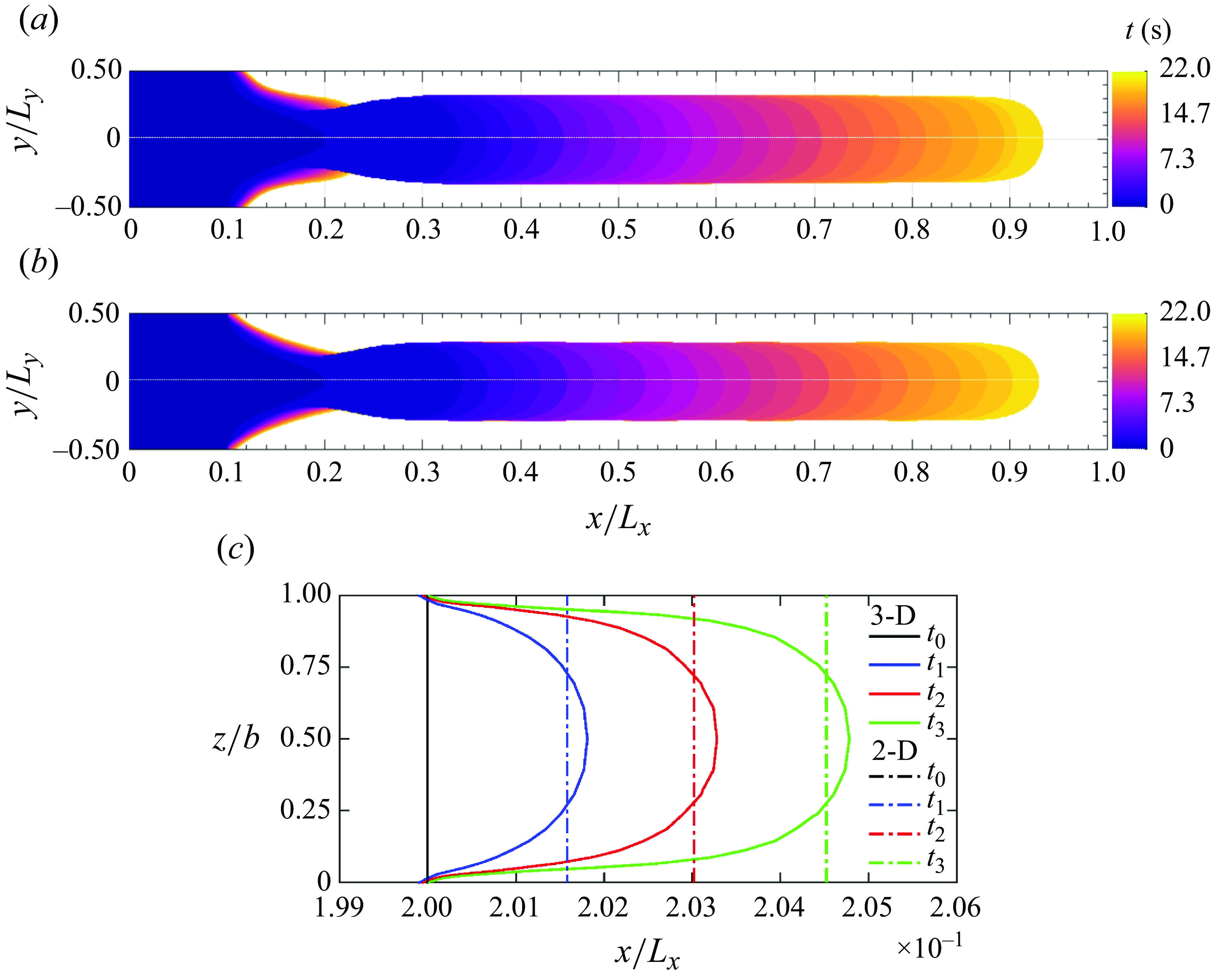
Figure 4. Evolution of the invading fluid finger for $(a)$
3-D and
$(a)$
3-D and $(b)$
2-D simulations, with
$(b)$
2-D simulations, with $u_{{in}} = 2.0\times 10^{-3}$
m s−1,
$u_{{in}} = 2.0\times 10^{-3}$
m s−1, $Re=0.016$
and
$Re=0.016$
and $\log (Ca)=-3.18$
. Each location within the flow domain that is reached by the finger at some time is coloured according to that time, as indicated by the colour scale.
$\log (Ca)=-3.18$
. Each location within the flow domain that is reached by the finger at some time is coloured according to that time, as indicated by the colour scale. $(c)$
Vertical profiles of the fluid–fluid interface in the longitudinal vertical mid-plane of the flow cell, comparing early stages of 3-D (solid curves) and 2-D (dashed lines) simulations. The initial interface position (
$(c)$
Vertical profiles of the fluid–fluid interface in the longitudinal vertical mid-plane of the flow cell, comparing early stages of 3-D (solid curves) and 2-D (dashed lines) simulations. The initial interface position ( $t_0 = 0 \text{ s}$
) is shown by the vertical black line. Coloured lines represent interface positions at
$t_0 = 0 \text{ s}$
) is shown by the vertical black line. Coloured lines represent interface positions at $t_1 = 0.04 \text{ s}$
,
$t_1 = 0.04 \text{ s}$
, $t_2 = 0.08 \text{ s}$
and
$t_2 = 0.08 \text{ s}$
and $t_3 = 0.12 \text{ s}$
.
$t_3 = 0.12 \text{ s}$
.
Next, we analyse how the ratio of the finger width to the flow cell width, $\lambda$
, varies with the capillary number
$\lambda$
, varies with the capillary number $Ca$
(figure 5). The 2-D simulations underpredict the finger width compared with their 3-D counterparts all the more as
$Ca$
(figure 5). The 2-D simulations underpredict the finger width compared with their 3-D counterparts all the more as $Ca$
is smaller, with the discrepancy being obvious for
$Ca$
is smaller, with the discrepancy being obvious for $Ca \lesssim 2.0 \times 10^{-3}$
. This is primarily due to the 2-D model’s limitations in capturing capillary forces, particularly in regions of the interface with complex geometries, such as the neck (near the inlet) or the regions where the lateral finger boundaries meet the top and bottom plates (for details see figure 5 of our recent work (Krishna et al. Reference Krishna, Méheust and Neuweiler2024)). In the Hele-Shaw geometry, local discrepancies in capillary forces between the 3-D model and the depth-integrated model impact the fluid distribution in the whole medium. Notably, closely spaced data points at the same
$Ca \lesssim 2.0 \times 10^{-3}$
. This is primarily due to the 2-D model’s limitations in capturing capillary forces, particularly in regions of the interface with complex geometries, such as the neck (near the inlet) or the regions where the lateral finger boundaries meet the top and bottom plates (for details see figure 5 of our recent work (Krishna et al. Reference Krishna, Méheust and Neuweiler2024)). In the Hele-Shaw geometry, local discrepancies in capillary forces between the 3-D model and the depth-integrated model impact the fluid distribution in the whole medium. Notably, closely spaced data points at the same $Ca$
represent simulations performed with different grid resolutions:
$Ca$
represent simulations performed with different grid resolutions: $b/\Delta x = 4$
,
$b/\Delta x = 4$
, $8$
and
$8$
and $16$
, where
$16$
, where $\Delta x= \Delta y$
is the uniform cell size in the
$\Delta x= \Delta y$
is the uniform cell size in the $xy$
plane. As a secondary criterion for grid convergence, pressure drops across the channel were also examined. Since the difference in results between
$xy$
plane. As a secondary criterion for grid convergence, pressure drops across the channel were also examined. Since the difference in results between $b/\Delta x = 8$
and
$b/\Delta x = 8$
and $16$
was under
$16$
was under $2\,\% - 4\, \%$
, we chose a horizontal discretisation level of
$2\,\% - 4\, \%$
, we chose a horizontal discretisation level of $b/\Delta x = 8$
for all simulations.
$b/\Delta x = 8$
for all simulations.
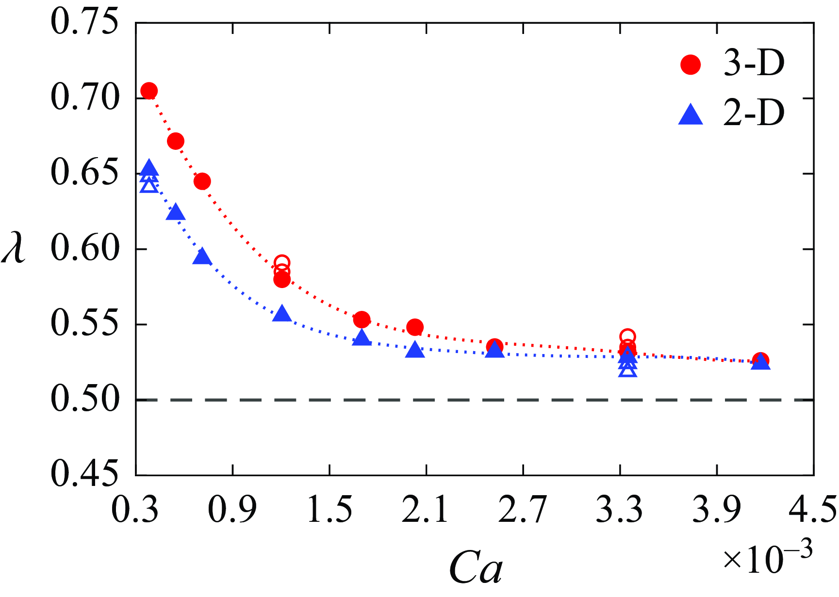
Figure 5. Relationship between the finger width normalised by the channel width, $\lambda$
, and the capillary number (
$\lambda$
, and the capillary number ( $Ca$
), for the 3-D simulations (red circles) and 2-D simulations (blue triangles). When several symbols are visible at a given
$Ca$
), for the 3-D simulations (red circles) and 2-D simulations (blue triangles). When several symbols are visible at a given $Ca$
, they represent simulations with different mesh resolutions. Filled symbols indicate simulations where grid convergence was achieved, while empty symbols correspond to intermediate grid refinement stages. The dotted curves joining the data points represents a curve of best fit.
$Ca$
, they represent simulations with different mesh resolutions. Filled symbols indicate simulations where grid convergence was achieved, while empty symbols correspond to intermediate grid refinement stages. The dotted curves joining the data points represents a curve of best fit.
Under the assumption of a 2-D flow and neglecting surface tension effects, Saffman & Taylor (Reference Saffman and Taylor1958) derived a parametric equation for the shape of a single finger in the horizontal plane
 \begin{equation} \bar {x} = \frac {1-\lambda }{\pi } \ln \frac {1}{2}\left ( 1 + \cos \frac {\pi \bar {y}}{\lambda }\right). \end{equation}
Here, $\bar {x}$
and
$\bar {x}$
and $\bar {y}$
are dimensionless coordinates normalised by the channel width
$\bar {y}$
are dimensionless coordinates normalised by the channel width $L_y$
, and
$L_y$
, and $\lambda$
is a free parameter corresponding to the width of the finger normalised by
$\lambda$
is a free parameter corresponding to the width of the finger normalised by $L_y$
; it is not prescribed by the theoretical derivation. In figure 6, we compare such analytical profiles to numerical simulations, with
$L_y$
; it is not prescribed by the theoretical derivation. In figure 6, we compare such analytical profiles to numerical simulations, with $\lambda$
fitted to the width of the numerically predicted finger, for two extreme flow cases:
$\lambda$
fitted to the width of the numerically predicted finger, for two extreme flow cases: $\log (Ca) = -2.48$
,
$\log (Ca) = -2.48$
, $Re = 0.08$
(figure 6
a), and
$Re = 0.08$
(figure 6
a), and $\log (Ca) = -3.48$
and
$\log (Ca) = -3.48$
and $Re = 0.008$
(figure 6
b). While at higher
$Re = 0.008$
(figure 6
b). While at higher $Ca$
, both the 3-D and 2-D analytical finger profiles show excellent match to the numerical data, at lower
$Ca$
, both the 3-D and 2-D analytical finger profiles show excellent match to the numerical data, at lower $Ca$
, when surface tension effects are 10 times more important, significant discrepancies between the 3-D numerical and analytical solutions become apparent.
$Ca$
, when surface tension effects are 10 times more important, significant discrepancies between the 3-D numerical and analytical solutions become apparent.
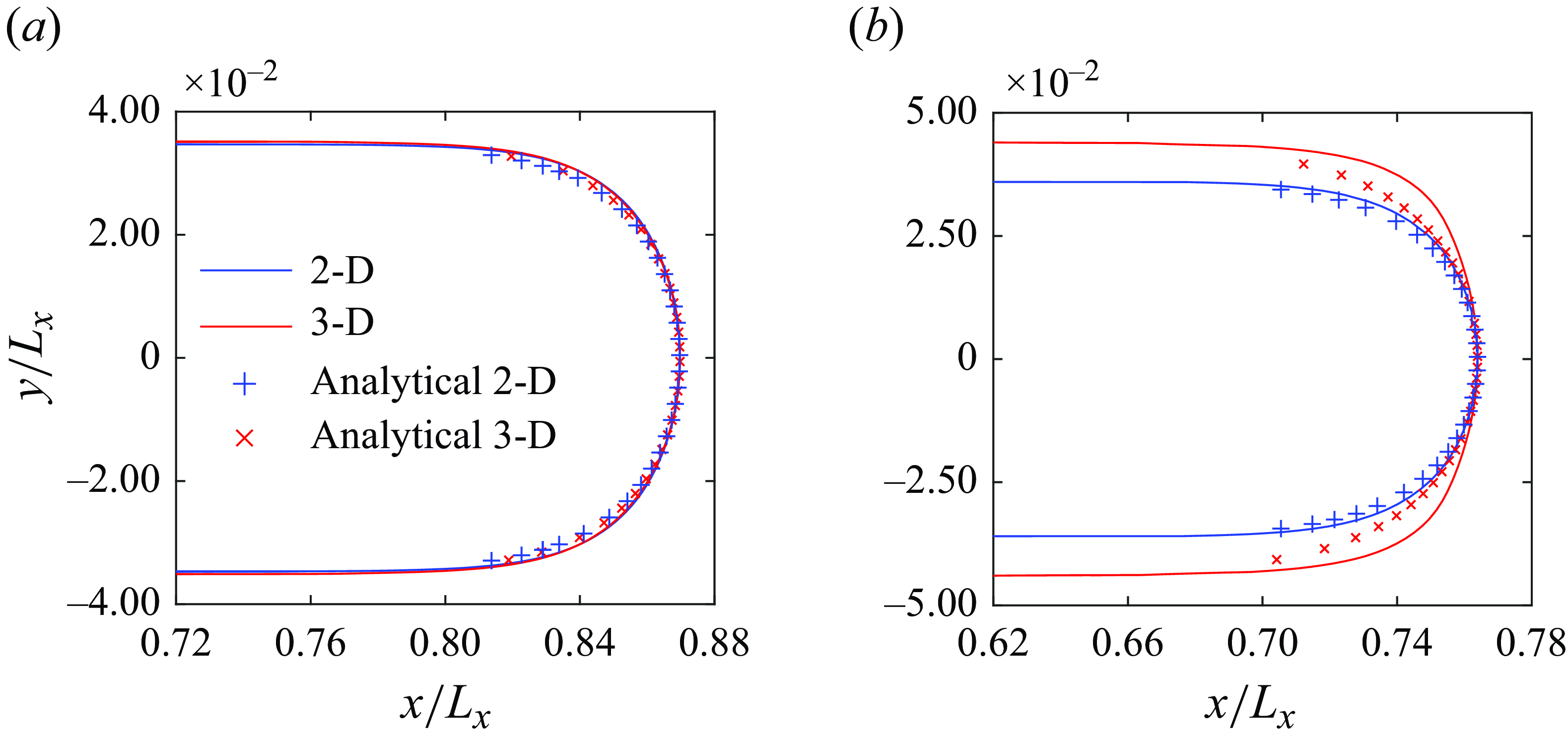
Figure 6. Comparison of the horizontal profile of the finger front (for the 3-D model, in the horizontal mid-plane, $(z=b/2)$
, of the flow cell) obtained from numerical simulations (solid curves) with the analytical solution of Saffman & Taylor (Reference Saffman and Taylor1958) (markers) with finger width fitted either to the 2-D (‘Analytical 2-D’) or to the 3-D (‘Analytical 3-D’) numerical data. The flow conditions for
$(z=b/2)$
, of the flow cell) obtained from numerical simulations (solid curves) with the analytical solution of Saffman & Taylor (Reference Saffman and Taylor1958) (markers) with finger width fitted either to the 2-D (‘Analytical 2-D’) or to the 3-D (‘Analytical 3-D’) numerical data. The flow conditions for $(a)$
are:
$(a)$
are: $U = 1.0\times 10^{-2}$
ms–1,
$U = 1.0\times 10^{-2}$
ms–1, $\log (Ca) = -2.48$
and
$\log (Ca) = -2.48$
and $Re = 0.08$
, and for the
$Re = 0.08$
, and for the $(b)$
they are:
$(b)$
they are: $U = 1.0\times 10^{-3}$
ms–1,
$U = 1.0\times 10^{-3}$
ms–1, $\log (Ca) = -3.48$
and
$\log (Ca) = -3.48$
and $Re = 0.008$
.
$Re = 0.008$
.
Breakthrough times: the breakthrough time, $t^*$
, refers to the time taken for the invading fluid to reach the outlet. Figure 7 presents the relative differences in breakthrough times between the 3-D and 2-D simulations across the full range of
$t^*$
, refers to the time taken for the invading fluid to reach the outlet. Figure 7 presents the relative differences in breakthrough times between the 3-D and 2-D simulations across the full range of $Ca$
values. The 3-D simulations consistently predict lower breakthrough times than the 2-D simulations. The presence of a wetting film in the 3-D configuration reduces the effective aperture available for the invading fluid finger, and, in addition, ensures slip velocity conditions at the top and bottom boundaries of the injected fluid domain, rather than no-flow boundaries; hence, the finger’s motion is expected to be faster than for the 2-D simulation. Notably, as
$Ca$
values. The 3-D simulations consistently predict lower breakthrough times than the 2-D simulations. The presence of a wetting film in the 3-D configuration reduces the effective aperture available for the invading fluid finger, and, in addition, ensures slip velocity conditions at the top and bottom boundaries of the injected fluid domain, rather than no-flow boundaries; hence, the finger’s motion is expected to be faster than for the 2-D simulation. Notably, as $Ca$
decreases and the film thickness diminishes, the relative difference in breakthrough times reduces, approaching approximately
$Ca$
decreases and the film thickness diminishes, the relative difference in breakthrough times reduces, approaching approximately $1\, \%$
for the lowest investigated
$1\, \%$
for the lowest investigated $Ca$
values.
$Ca$
values.
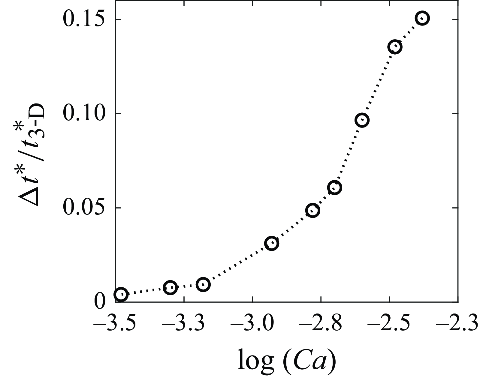
Figure 7. Dependence of the relative differences in breakthrough times between the 3-D and 2-D simulations, $\Delta t^*/ t^*_{\textrm{3D}} = t^*_{\textrm{2D}}/t^*_{\textrm{3D}} - 1$
, plotted against
$\Delta t^*/ t^*_{\textrm{3D}} = t^*_{\textrm{2D}}/t^*_{\textrm{3D}} - 1$
, plotted against $\log (Ca)$
.
$\log (Ca)$
.
Macroscopic pressure drop: we now evaluate the 2-D model’s ability to predict pressure drops across the inlet–outlet boundaries in comparison with the 3-D model’s results. With the outlet pressure set to $0$
Pa, the area-weighted average pressure drop
$0$
Pa, the area-weighted average pressure drop $\Delta P_{{io}}$
across the channel is defined as (Ferrari & Lunati Reference Ferrari and Lunati2013; Chen et al. Reference Chen, Guo, Wu and Hu2018; Krishna et al. Reference Krishna, Méheust and Neuweiler2024)
$\Delta P_{{io}}$
across the channel is defined as (Ferrari & Lunati Reference Ferrari and Lunati2013; Chen et al. Reference Chen, Guo, Wu and Hu2018; Krishna et al. Reference Krishna, Méheust and Neuweiler2024)
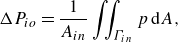 \begin{equation} \Delta P_{{io}} = \frac {1}{A_{{in}}}\iint _{\Gamma _{{in}}} p \, \text{d}A, \end{equation}
where $A_{{in}}$
and
$A_{{in}}$
and $\Gamma _{{in}}$
represent the inlet area and inlet boundary, respectively. For the four representative flow conditions listed in table 1, figure 8(a) shows the dependence of
$\Gamma _{{in}}$
represent the inlet area and inlet boundary, respectively. For the four representative flow conditions listed in table 1, figure 8(a) shows the dependence of $\Delta P_{{io}}$
as a function of the global saturation
$\Delta P_{{io}}$
as a function of the global saturation $S_1$
, which is the fraction of the total domain volume occupied by fluid 1
$S_1$
, which is the fraction of the total domain volume occupied by fluid 1
 \begin{equation} S_1 = \tfrac {1}{V}\int _V \gamma \text{d}V. \end{equation}
In effect, since the volumetric flow rate is constant over time, $S_1$
is linearly related to the ratio of time to breakthrough time. In figure 8(a), a linear drop in pressure is observed as the less viscous fluid gradually displaces the more viscous one. Figure 8(b) shows the longitudinal pressure drop along the longitudinal mid-line of the channel (
$S_1$
is linearly related to the ratio of time to breakthrough time. In figure 8(a), a linear drop in pressure is observed as the less viscous fluid gradually displaces the more viscous one. Figure 8(b) shows the longitudinal pressure drop along the longitudinal mid-line of the channel ( $y=0$
) when the invading fluid has reached 60 % of the channel length. At high
$y=0$
) when the invading fluid has reached 60 % of the channel length. At high $Ca$
, the pressure drop near the inlet, and in the region occupied by fluid 1, is nonlinear due to the narrow finger and the effects of capillary forces. However, farther from the inlet, the pressure drop becomes linear; this is expected as the displacing fluid, of constant viscosity, is displaced with a uniform and stationary velocity along that line. In the more viscous displaced fluid, for the same reason, a linear pressure drop is observed, but with a stronger absolute pressure gradient due to the higher fluid viscosity. A close-to-vertical drop corresponding to the capillary pressure across the fluid–fluid interface separates these two linear regimes. Both the time evolution of the macroscopic pressure drop (figure 8
a) and the longitudinal pressure profiles obtained with the 2-D model (figure 8
b) closely align with the 3-D results, with a degree of alignment that is all the higher as
$Ca$
, the pressure drop near the inlet, and in the region occupied by fluid 1, is nonlinear due to the narrow finger and the effects of capillary forces. However, farther from the inlet, the pressure drop becomes linear; this is expected as the displacing fluid, of constant viscosity, is displaced with a uniform and stationary velocity along that line. In the more viscous displaced fluid, for the same reason, a linear pressure drop is observed, but with a stronger absolute pressure gradient due to the higher fluid viscosity. A close-to-vertical drop corresponding to the capillary pressure across the fluid–fluid interface separates these two linear regimes. Both the time evolution of the macroscopic pressure drop (figure 8
a) and the longitudinal pressure profiles obtained with the 2-D model (figure 8
b) closely align with the 3-D results, with a degree of alignment that is all the higher as $Ca$
is smaller.
$Ca$
is smaller.
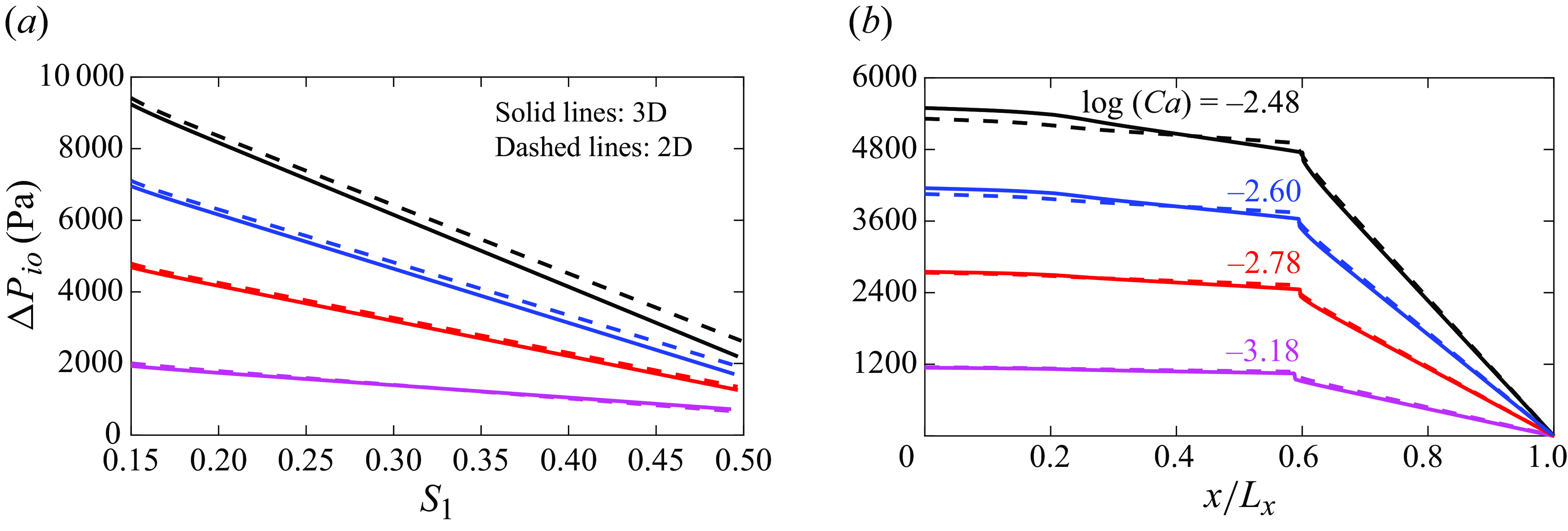
Figure 8. Comparison of pressure drops: (a) the area-weighted average pressure drop $\Delta P_{{io}}$
along the Hele-Shaw channel, plotted against the global saturation
$\Delta P_{{io}}$
along the Hele-Shaw channel, plotted against the global saturation $S_1$
of the invading fluid 1; (b) the longitudinal pressure profile
$S_1$
of the invading fluid 1; (b) the longitudinal pressure profile $\Delta P$
along the longitudinal centreline from the inlet
$\Delta P$
along the longitudinal centreline from the inlet $(x=0,:y=0,:z=b/2)$
to the outlet
$(x=0,:y=0,:z=b/2)$
to the outlet $(x=L_x,:y=0,:z=b/2)$
, when the invading finger covers
$(x=L_x,:y=0,:z=b/2)$
, when the invading finger covers $60\, \%$
of the channel length. These results are shown for four different capillary numbers. The solid and the dashed curves represent respectively the 3-D and 2-D results, while the corresponding
$60\, \%$
of the channel length. These results are shown for four different capillary numbers. The solid and the dashed curves represent respectively the 3-D and 2-D results, while the corresponding $\log (Ca)$
values are indicated with coloured text in panel
$\log (Ca)$
values are indicated with coloured text in panel $(b)$
.
$(b)$
.
Vertical velocity profiles: lastly, to test the validity of our assumption of a vertical parabolic velocity profile, employed to model the wall shear stress term $\boldsymbol{\tau _{w}}$
in our 2-D model (3.17), we examine the
$\boldsymbol{\tau _{w}}$
in our 2-D model (3.17), we examine the $x$
component of the velocity at two specific
$x$
component of the velocity at two specific $x$
positions along the longitudinal mid-plane of the flow cell, one on each side of the interface, positioned sufficiently away from the fingertip. In figure 9 such profiles are shown for two distinct flow rates, corresponding respectively to
$x$
positions along the longitudinal mid-plane of the flow cell, one on each side of the interface, positioned sufficiently away from the fingertip. In figure 9 such profiles are shown for two distinct flow rates, corresponding respectively to $\log (Ca)=-3.48$
and
$\log (Ca)=-3.48$
and $Re = 0.008$
(slow), and
$Re = 0.008$
(slow), and $\log (Ca)=-2.48$
and
$\log (Ca)=-2.48$
and $Re = 0.08$
(fast), and for a time at which the fingertip has reached approximately half of the channel length. Note that: (i) the same profiles would be obtained at any different time provided the profiles are chosen at the same distance from the fingertip, (ii) the velocity whose
$Re = 0.08$
(fast), and for a time at which the fingertip has reached approximately half of the channel length. Note that: (i) the same profiles would be obtained at any different time provided the profiles are chosen at the same distance from the fingertip, (ii) the velocity whose $x$
-component is plotted has no
$x$
-component is plotted has no $y$
component, due to the symmetry of the finger. In both cases, the velocities within the defending fluid 2 region align perfectly with the dashed parabolic curve (figure 9
b). Within the region occupied by the invading fluid 1, it is observed that at the walls where a film of fluid 2 exists, the velocity magnitudes are smaller. Moving away from the walls, higher gradients in velocity are encountered, reaching a maximum value at the centre (figure 9
a). When disregarding the near-wall points with low-velocity gradients, the slower case exhibits a parabolic velocity profile. However, for the faster case, deviation from the parabolic profile is noticeable towards the centre. At higher inflow speeds, due to the increased wetting-film thickness, a departure from the parabolic distribution is evident in the observed velocity profiles.
$y$
component, due to the symmetry of the finger. In both cases, the velocities within the defending fluid 2 region align perfectly with the dashed parabolic curve (figure 9
b). Within the region occupied by the invading fluid 1, it is observed that at the walls where a film of fluid 2 exists, the velocity magnitudes are smaller. Moving away from the walls, higher gradients in velocity are encountered, reaching a maximum value at the centre (figure 9
a). When disregarding the near-wall points with low-velocity gradients, the slower case exhibits a parabolic velocity profile. However, for the faster case, deviation from the parabolic profile is noticeable towards the centre. At higher inflow speeds, due to the increased wetting-film thickness, a departure from the parabolic distribution is evident in the observed velocity profiles.
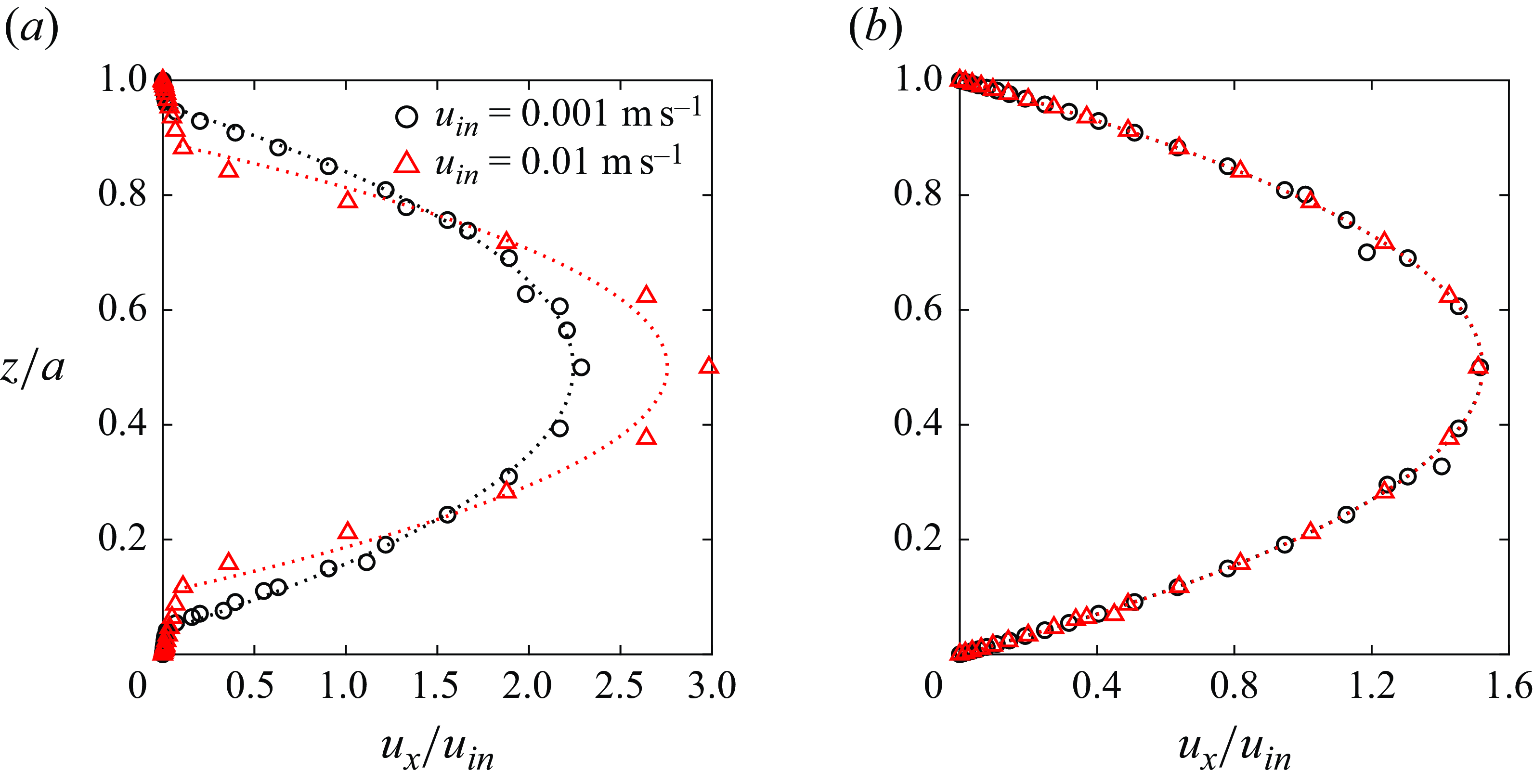
Figure 9. Vertical profiles of 3-D velocity component ( $x$
component) plotted at two distinct positions along the longitudinal mid-plane of the Hele-Shaw cell:
$x$
component) plotted at two distinct positions along the longitudinal mid-plane of the Hele-Shaw cell: $(a)$
$(a)$ $(0.045, 0.0)$
m and
$(0.045, 0.0)$
m and $(b)$
$(b)$ $(0.08, 0.0)$
m, occupied by fluid 1 and fluid 2 respectively, and located sufficiently away from the interface at a time when the interface tip has approximately reached half the length of the flow channel. The flow conditions for these profiles are:
$(0.08, 0.0)$
m, occupied by fluid 1 and fluid 2 respectively, and located sufficiently away from the interface at a time when the interface tip has approximately reached half the length of the flow channel. The flow conditions for these profiles are: $u_{{in}} = 1$
mm/s,
$u_{{in}} = 1$
mm/s, $\log (Ca) = -3.48$
,
$\log (Ca) = -3.48$
, $Re = 0.008$
at
$Re = 0.008$
at $t = 12$
s denoted by black circles, and
$t = 12$
s denoted by black circles, and $u_{{in}} = 10$
mm s–1,
$u_{{in}} = 10$
mm s–1, $\log (Ca) = -2.48$
,
$\log (Ca) = -2.48$
, $Re = 0.08$
at
$Re = 0.08$
at $t = 2$
s denoted by red triangles. The dotted curves represent the corresponding best-fit parabolic profiles.
$t = 2$
s denoted by red triangles. The dotted curves represent the corresponding best-fit parabolic profiles.
Conclusion on the model validation: in this section, we have carried out a comparison of our derived two-phase 2-D depth-integrated model’s predictions with the full 3-D model results as well as to analytical solutions, in order to validate the approach and identify limitations. The 2-D model could accurately predict all relevant key macroscopic flow quantities, such as the finger pattern and pressure drops. As the flow $Re$
increases, our assumption of a parabolic velocity profile becomes less accurate, leading to discrepancies in the representation of wall shear stress and thus of the pressure drops. The discrepancies in pressure are, however, very small. On the other hand, as
$Re$
increases, our assumption of a parabolic velocity profile becomes less accurate, leading to discrepancies in the representation of wall shear stress and thus of the pressure drops. The discrepancies in pressure are, however, very small. On the other hand, as $Ca$
gets below
$Ca$
gets below $10^{-4}$
, where surface tension effects become more important, the 2-D model’s interface representation falls short of fully capturing the localised 3-D effects, leading to deviations of the finger shapes in such a way that the finger width is slightly underpredicted.
$10^{-4}$
, where surface tension effects become more important, the 2-D model’s interface representation falls short of fully capturing the localised 3-D effects, leading to deviations of the finger shapes in such a way that the finger width is slightly underpredicted.
4.3. Results for numerical experiments in rough fractures
In this section, we investigate the predictions of the two-phase 2-D model on a fracture geometry, where complex spatial variations in the fracture’s local apertures come into play.
4.3.1. Fracture geometry
Figure 10(a) depicts the schematics of the numerically generated rough fracture used to carry out our drainage simulations. It consists of a top and bottom wall with parallel horizontal mean planes, separated by a mean aperture distance of $\bar {a}$
(the walls do not come into contact). The fracture features self-affine isotropic topographies for the top and bottom walls, exhibiting long-range correlations characterised by the Hurst exponent
$\bar {a}$
(the walls do not come into contact). The fracture features self-affine isotropic topographies for the top and bottom walls, exhibiting long-range correlations characterised by the Hurst exponent $H$
(here
$H$
(here $H=0.8$
) (Plouraboué et al. Reference Plouraboué, Kurowski, Hulin, Roux and Schmittbuhl1995; Bouchaud Reference Bouchaud1997). The two walls share identical large-scale variations above a characteristic length
$H=0.8$
) (Plouraboué et al. Reference Plouraboué, Kurowski, Hulin, Roux and Schmittbuhl1995; Bouchaud Reference Bouchaud1997). The two walls share identical large-scale variations above a characteristic length $L_{{c}}$
, denoted as the correlation length. In addition to parameters (i)
$L_{{c}}$
, denoted as the correlation length. In addition to parameters (i) $\bar {a}$
, (ii)
$\bar {a}$
, (ii) $H$
and (iii)
$H$
and (iii) $L_{{c}}$
, the aperture field of the fracture is primarily defined by (iv) its standard deviation
$L_{{c}}$
, the aperture field of the fracture is primarily defined by (iv) its standard deviation $\sigma _{{a}}$
and (v) the horizontal dimensions
$\sigma _{{a}}$
and (v) the horizontal dimensions $L_x$
and
$L_x$
and $L_y$
of the fracture (Méheust & Schmittbuhl Reference Méheust and Schmittbuhl2003; Dewangan et al. Reference Dewangan, Ghosh, Le Borgne and Méheust2022). For further insights into the geometrical properties of such geological fractures, see Lenci et al. (Reference Lenci, Putti, Di Federico and Méheust2022) and Dewangan et al. (Reference Dewangan, Ghosh, Le Borgne and Méheust2022). The topographies of the fracture walls were generated using the spectral method described by Méheust & Schmittbuhl (Reference Méheust and Schmittbuhl2003). The resulting aperture field is shown as a contour plot in figure 10(b), while a similar representation of the average surface (at equal distance from the two walls) of the fracture is shown in figure 10(d).
$L_y$
of the fracture (Méheust & Schmittbuhl Reference Méheust and Schmittbuhl2003; Dewangan et al. Reference Dewangan, Ghosh, Le Borgne and Méheust2022). For further insights into the geometrical properties of such geological fractures, see Lenci et al. (Reference Lenci, Putti, Di Federico and Méheust2022) and Dewangan et al. (Reference Dewangan, Ghosh, Le Borgne and Méheust2022). The topographies of the fracture walls were generated using the spectral method described by Méheust & Schmittbuhl (Reference Méheust and Schmittbuhl2003). The resulting aperture field is shown as a contour plot in figure 10(b), while a similar representation of the average surface (at equal distance from the two walls) of the fracture is shown in figure 10(d).
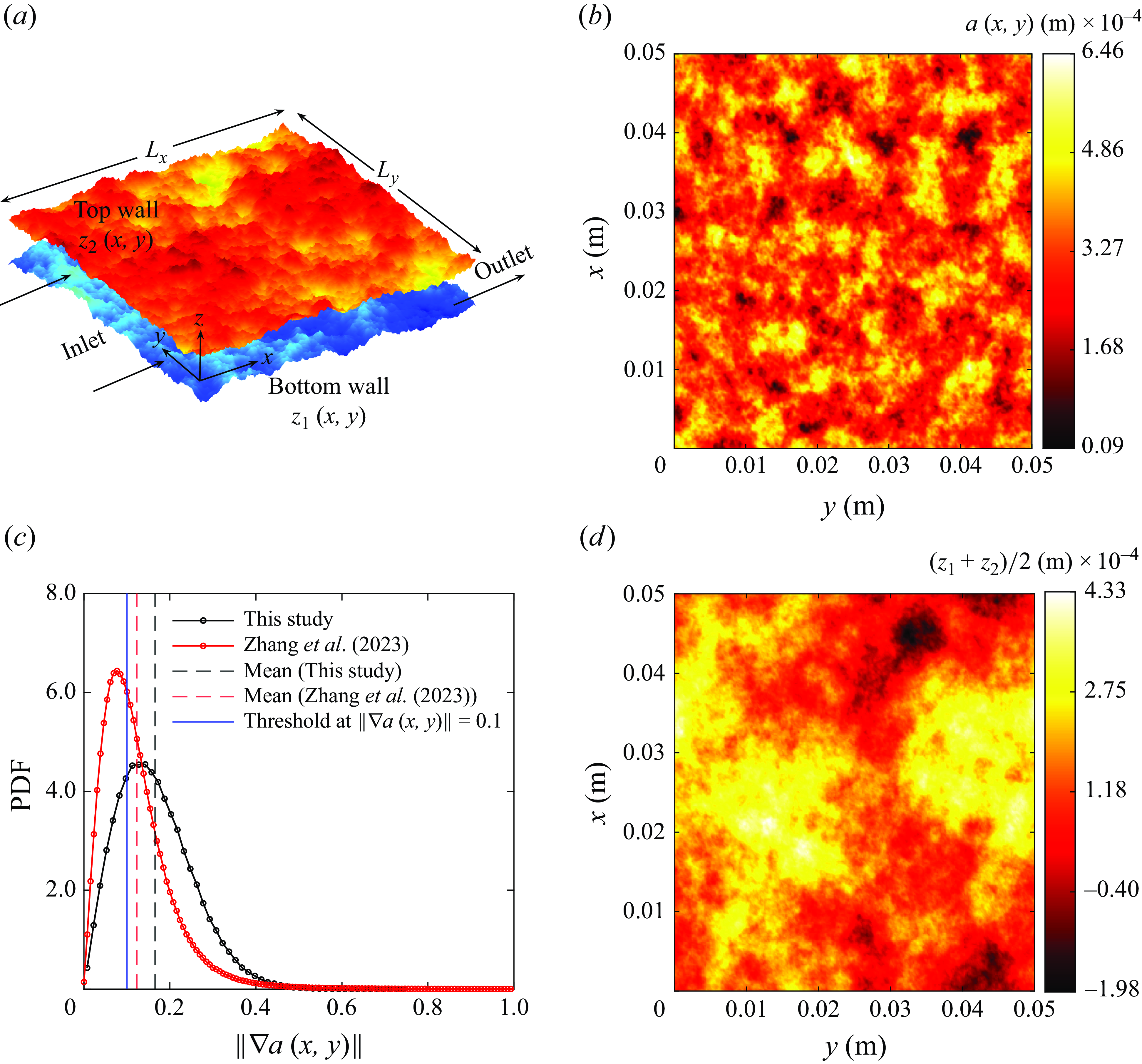
Figure 10. (a) Schematic of the synthetic rough fracture with self-affine top and bottom walls characterised by a Hurst exponent of $H=0.8$
. The horizontal dimensions are
$H=0.8$
. The horizontal dimensions are $L_x = L_y = 0.05$
m, where
$L_x = L_y = 0.05$
m, where $(x\in [0, L_x])$
and
$(x\in [0, L_x])$
and $(y\in [0,L_y])$
. The fracture has a correlation length of
$(y\in [0,L_y])$
. The fracture has a correlation length of $L_c = L_x/4 = 0.0125$
m, with a mean aperture
$L_c = L_x/4 = 0.0125$
m, with a mean aperture $\bar {a} = 3.3\times 10^{-4}$
m, a standard deviation
$\bar {a} = 3.3\times 10^{-4}$
m, a standard deviation $\sigma _{{a}} = 90$
µm and a mean inlet aperture
$\sigma _{{a}} = 90$
µm and a mean inlet aperture $\bar {a}_{{in}} = 3.2\times 10^{-4}$
m. (b) Aperture field
$\bar {a}_{{in}} = 3.2\times 10^{-4}$
m. (b) Aperture field $a(x,y)$
of the fracture. (c) Probability density function (PDF) of the aperture field gradient,
$a(x,y)$
of the fracture. (c) Probability density function (PDF) of the aperture field gradient, $\|\nabla a(x,y)\|$
(black symbols and line), with that from a replica of natural fracture (Zhang et al. Reference Zhang, Yang, Méheust, Neuweiler, Hu and Chen2023); the corresponding mean aperture gradient values are also shown for both PDFs, as well as the 0.1 threshold corresponding to the strict lubrication approximation. (d) Map of the mean fracture topography,
$\|\nabla a(x,y)\|$
(black symbols and line), with that from a replica of natural fracture (Zhang et al. Reference Zhang, Yang, Méheust, Neuweiler, Hu and Chen2023); the corresponding mean aperture gradient values are also shown for both PDFs, as well as the 0.1 threshold corresponding to the strict lubrication approximation. (d) Map of the mean fracture topography, $(z_1+z_2)/2$
.
$(z_1+z_2)/2$
.
The generated top and bottom wall topographies consisted of $512\times 512$
points each, resulting in a horizontal
$512\times 512$
points each, resulting in a horizontal $xy$
resolution of
$xy$
resolution of $97$
µm. Note that:
$97$
µm. Note that:
-
(i) The probability density function (PDF) of the aperture gradient, shown as black line and symbols in figure 10(c), is significantly wider than what the strict lubrication approximation requires (blue vertical line), in particular the mean aperture gradient magnitude is $0.17 \pm 0.01$
, hence a satisfying agreement between the depth-integrated model’s predictions and those from corresponding 3-D simulations will show that the depth-integrated model can even be applied to geometries that do not strictly adhere to the lubrication approximation. In fact, the PDF shown in red, computed from the replica of a natural fracture (Zhang et al. Reference Zhang, Yang, Méheust, Neuweiler, Hu and Chen2023) is narrower than that of our synthetic geological fracture, with a mean gradient magnitude of
$0.12 \pm 0.01$
; thus, the depth-integrated model is likely able to properly address real fracture geometries.
$0.17 \pm 0.01$
, hence a satisfying agreement between the depth-integrated model’s predictions and those from corresponding 3-D simulations will show that the depth-integrated model can even be applied to geometries that do not strictly adhere to the lubrication approximation. In fact, the PDF shown in red, computed from the replica of a natural fracture (Zhang et al. Reference Zhang, Yang, Méheust, Neuweiler, Hu and Chen2023) is narrower than that of our synthetic geological fracture, with a mean gradient magnitude of
$0.12 \pm 0.01$
; thus, the depth-integrated model is likely able to properly address real fracture geometries. -
(ii) Due to the self-affinity of the wall roughness at scales smaller than
$L_{{c}}$
, the resolution of the aperture field may influence the flow dynamics as insufficient resolution leads to not accounting for smaller-scale roughness in the numerical geometry, affecting the small-scale complexity of the simulated flow; see e.g. Wang et al. (Reference Wang, Bao, Pereira, Sauret and Gan2022) for an illustration of this effect in single-phase flow and its impact on the estimated permeability. To ensure accuracy, we analysed the effect of aperture field resolution on invasion patterns and flow metrics for both the 3-D and 2-D models. This analysis, detailed in Appendix D, confirmed that the
$97$
µm resolution used in this study captures the geometry at sufficiently small scales (i.e. at scales that are sufficiently smaller than
$L_{{c}}$
) for the essential flow physics to be accounted for, with negligible differences to predictions obtained at even finer resolutions.


4.3.2. Numerical set-up and flow conditions
For the drainage simulations within the rough fracture geometry, we use a set-up similar to that described in Appendix 4.2, where a less viscous fluid 1 displaces a more viscous fluid 2. To accurately capture the onset of instability of the fluid–fluid interface, the interface is initialised a small distance of $0.0025$
m (
$0.0025$
m ( $=L_x/20$
) from the inlet, meaning that at
$=L_x/20$
) from the inlet, meaning that at $t=0$
, fluid 1 occupies a small portion of the fracture domain. The nomenclature for the different domain boundaries (as shown in figure 10
a) follows that of the Hele-Shaw channel, and the boundary conditions for the simulations remain consistent with those in table 2. We examine five different cases of
$t=0$
, fluid 1 occupies a small portion of the fracture domain. The nomenclature for the different domain boundaries (as shown in figure 10
a) follows that of the Hele-Shaw channel, and the boundary conditions for the simulations remain consistent with those in table 2. We examine five different cases of $Ca$
, covering three orders of magnitude:
$Ca$
, covering three orders of magnitude: $\log _{10} Ca = -3.0, -3.5, -4.0, -4.5, -5.0$
. Table 3 lists the corresponding inlet injection speeds
$\log _{10} Ca = -3.0, -3.5, -4.0, -4.5, -5.0$
. Table 3 lists the corresponding inlet injection speeds $u_{{in}} = \sigma Ca/\mu _1$
for these cases, along with the resulting
$u_{{in}} = \sigma Ca/\mu _1$
for these cases, along with the resulting $Re = \rho _1 u_{{in}} \bar {a}_{{in}} / \mu _1$
, where the inlet mean aperture
$Re = \rho _1 u_{{in}} \bar {a}_{{in}} / \mu _1$
, where the inlet mean aperture $\bar {a}_{{in}}$
is used to compute
$\bar {a}_{{in}}$
is used to compute $Re$
. In the case of the 2-D model, where the primary variable is the local flux
$Re$
. In the case of the 2-D model, where the primary variable is the local flux $\boldsymbol{Q} = (Q_x, Q_y)$
, the flux at the inlet boundary is defined as
$\boldsymbol{Q} = (Q_x, Q_y)$
, the flux at the inlet boundary is defined as $Q_{{in}} = u_{{in}} \times a(0,y)$
, resulting in a spatially varying inlet boundary condition. As in sub§ 4.2, we employ a mesh refinement near the top and bottom walls to capture the thin defending fluid film (see figure 11). Based on the Hele-Shaw validation (§ 4.2) and additional tests on smaller fracture domains, we determined that a horizontal discretisation of
$Q_{{in}} = u_{{in}} \times a(0,y)$
, resulting in a spatially varying inlet boundary condition. As in sub§ 4.2, we employ a mesh refinement near the top and bottom walls to capture the thin defending fluid film (see figure 11). Based on the Hele-Shaw validation (§ 4.2) and additional tests on smaller fracture domains, we determined that a horizontal discretisation of $\Delta x = 50$
µm is sufficient for a converged solution. The 2-D mesh, similar to figure 3(b), has only one cell in the
$\Delta x = 50$
µm is sufficient for a converged solution. The 2-D mesh, similar to figure 3(b), has only one cell in the $z$
direction, with no boundary conditions imposed at the top and bottom boundaries of the flow domain.
$z$
direction, with no boundary conditions imposed at the top and bottom boundaries of the flow domain.
Table 3. Fluid properties and flow parameters used for the drainage simulations in the rough fracture geometry.
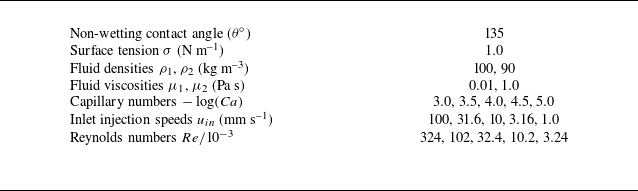
Figure 11. The 3-D computational mesh for the rough fracture geometry, with a grid size = $3.2 \times 10^7$ $(=1000 \times 1000 \times 32)$
. The horizontal discretisation corresponds to a cell size of
$(=1000 \times 1000 \times 32)$
. The horizontal discretisation corresponds to a cell size of $\Delta x = 50$
µm, while the vertical discretisation with
$\Delta x = 50$
µm, while the vertical discretisation with $32$
uniformly graded cells (
$32$
uniformly graded cells ( $1.33$
cell-to-cell expansion ratio) results in a mean cell thicknesses of
$1.33$
cell-to-cell expansion ratio) results in a mean cell thicknesses of $0.39$
µm. In the case of the 2-D computational mesh, the grid size is given as
$0.39$
µm. In the case of the 2-D computational mesh, the grid size is given as $1.0 \times 10^6$ $(1000 \times 1000 \times 1)$
.
$(1000 \times 1000 \times 1)$
.
4.3.3. Comparison of results of the 2-D depth-integrated model with those from the 3-D model
Invasion patterns: in the context of immiscible flow in fractured media, the fluid–fluid displacement pattern (or invasion morphology) is a crucial quantity of interest. It is governed by the competition between viscous and capillary forces, as well as the local aperture field. If the interface is viscously unstable ( $\mu _2/\mu _1 \gt 1$
), this interplay of forces gives rise to the emergence of finger-like patterns dominated by capillary fingering at low
$\mu _2/\mu _1 \gt 1$
), this interplay of forces gives rise to the emergence of finger-like patterns dominated by capillary fingering at low $Ca$
and viscous fingering at higher
$Ca$
and viscous fingering at higher $Ca$
, as originally defined in 2-D porous media, and more recently observed in rough fractures (Chen et al. Reference Chen, Fang, Wu and Hu2017). These two regimes of invasion patterns are distinguished by the presence of more irregular fingers with multi-directional growth in the case of capillary fingering, compared with more flow-aligned finger patterns in the case of viscous fingering. Figure 12 shows displacement morphologies in the mean fracture plane across different
$Ca$
, as originally defined in 2-D porous media, and more recently observed in rough fractures (Chen et al. Reference Chen, Fang, Wu and Hu2017). These two regimes of invasion patterns are distinguished by the presence of more irregular fingers with multi-directional growth in the case of capillary fingering, compared with more flow-aligned finger patterns in the case of viscous fingering. Figure 12 shows displacement morphologies in the mean fracture plane across different $Ca$
values. The images overlay invasion patterns, using distinct colours to indicate agreement (yellow) or discrepancy (blue and red) between patterns obtained from the 2-D and 3-D simulations. As seen for the Hele-Shaw configuration (§ 4.2.2), finger advancement times vary between the two models. Hence, for comparison, the snapshots for the patterns predicted by the 2-D and 3-D models are captured at different time steps, such that the advancing fingertips are approximately at the same distance from the outlet in the simulations.
$Ca$
values. The images overlay invasion patterns, using distinct colours to indicate agreement (yellow) or discrepancy (blue and red) between patterns obtained from the 2-D and 3-D simulations. As seen for the Hele-Shaw configuration (§ 4.2.2), finger advancement times vary between the two models. Hence, for comparison, the snapshots for the patterns predicted by the 2-D and 3-D models are captured at different time steps, such that the advancing fingertips are approximately at the same distance from the outlet in the simulations.
Figure 12. Invasion morphologies obtained in the synthetic geological fracture geometry from the 3-D and the 2-D model simulations. The three columns correspond to invasion patterns recorded at three different time steps at which the invading tip is located at around the same distance from the outlet boundary for the two models.
The rough fracture, whose geometry has been chosen so that its statistical properties are relevant to those of natural (in particular, subsurface) fractures, exhibits invasion patterns similar to those observed in such natural fractures (Chen et al. Reference Chen, Fang, Wu and Hu2017, Reference Chen, Guo, Wu and Hu2018). At smaller $Ca$
for which capillary forces become dominant, finger growth occurs in the transverse direction as well as the longitudinal direction, leading to broader fingers. This broadening reduces the number of fingers effectively advancing toward the outlet in comparison with higher
$Ca$
for which capillary forces become dominant, finger growth occurs in the transverse direction as well as the longitudinal direction, leading to broader fingers. This broadening reduces the number of fingers effectively advancing toward the outlet in comparison with higher $Ca$
cases. Notably, this behaviour is well predicted by the 2-D model. At larger capillary numbers (
$Ca$
cases. Notably, this behaviour is well predicted by the 2-D model. At larger capillary numbers ( $\log (Ca) \gt -4.0$
), discrepancies between the invasion patterns predicted by the two models primarily manifest in the extended blue regions (corresponding to predictions by the 3-D model) that align with the flow direction. As the invasion process advances, particularly in the later stages (e.g. figure 12
a
$\log (Ca) \gt -4.0$
), discrepancies between the invasion patterns predicted by the two models primarily manifest in the extended blue regions (corresponding to predictions by the 3-D model) that align with the flow direction. As the invasion process advances, particularly in the later stages (e.g. figure 12
a $^{{\prime }{\prime }}$
), these discrepancies become more pronounced, which is expected in processes driven by interface instabilities. The 2-D model cannot account for the presence of a wetting film, which is all the thicker as the capillary number is larger (a feature that is well predicted by the 3-D model). A relatively thick wetting film reduces the effective aperture space. Additionally, the wetting film alters the vertical position of the slip velocity boundary conditions at the top and bottom boundaries of the invading fluid domain. These factors jointly explain the differences between, the fingering patterns observed with the two models. In particular, at larger capillary numbers, the fingers predicted by the 3-D model tend to occupy more longitudinal space at any given time in comparison with their 2-D model counterparts. However, although there are small-scale features that are in these cases not reproduced by the 2-D model, the number of fingers and their larger-scale shape and location are well matched between the 3-D and 2-D models.
$^{{\prime }{\prime }}$
), these discrepancies become more pronounced, which is expected in processes driven by interface instabilities. The 2-D model cannot account for the presence of a wetting film, which is all the thicker as the capillary number is larger (a feature that is well predicted by the 3-D model). A relatively thick wetting film reduces the effective aperture space. Additionally, the wetting film alters the vertical position of the slip velocity boundary conditions at the top and bottom boundaries of the invading fluid domain. These factors jointly explain the differences between, the fingering patterns observed with the two models. In particular, at larger capillary numbers, the fingers predicted by the 3-D model tend to occupy more longitudinal space at any given time in comparison with their 2-D model counterparts. However, although there are small-scale features that are in these cases not reproduced by the 2-D model, the number of fingers and their larger-scale shape and location are well matched between the 3-D and 2-D models.
At smaller $Ca$
values, and thus, smaller wetting-film thicknesses, the agreement between the 2-D and 3-D patterns is better. However, we notice that the 2-D patterns differ from the 3-D ones at small scales. This is likely due to higher aperture gradients encountered locally within the flow domain (as seen in figure 10
c). Consequently, the out-of-plane curvature of the interface plays a significant role in determining pore occupancy – a factor that the 2-D model accounts for less accurately. Nevertheless, despite the inherent assumptions and simplifications, the 2-D model consistently captures the invasion morphology over larger length scales, in close agreement with the results obtained from the full 3-D model. In the following, we examine the 2-D model’s predictive capabilities for other hydrodynamic-scale and macroscopic flow observables.
$Ca$
values, and thus, smaller wetting-film thicknesses, the agreement between the 2-D and 3-D patterns is better. However, we notice that the 2-D patterns differ from the 3-D ones at small scales. This is likely due to higher aperture gradients encountered locally within the flow domain (as seen in figure 10
c). Consequently, the out-of-plane curvature of the interface plays a significant role in determining pore occupancy – a factor that the 2-D model accounts for less accurately. Nevertheless, despite the inherent assumptions and simplifications, the 2-D model consistently captures the invasion morphology over larger length scales, in close agreement with the results obtained from the full 3-D model. In the following, we examine the 2-D model’s predictive capabilities for other hydrodynamic-scale and macroscopic flow observables.
Breakthrough times: the differences in the breakthrough times ( $t^*$
) predicted by the 2-D and 3-D simulations are shown in figure 13. Consistently with our observations of the Saffman–Taylor finger growth (§ 4.2.2), the 2-D model overestimates
$t^*$
) predicted by the 2-D and 3-D simulations are shown in figure 13. Consistently with our observations of the Saffman–Taylor finger growth (§ 4.2.2), the 2-D model overestimates $t^*$
in comparison with the 3-D model predictions. However, this difference is substantially smaller at lower
$t^*$
in comparison with the 3-D model predictions. However, this difference is substantially smaller at lower $Ca$
values (
$Ca$
values ( $\log (Ca)\leqslant -4.0$
), again due to the reduced film thicknesses in the 3-D simulations.
$\log (Ca)\leqslant -4.0$
), again due to the reduced film thicknesses in the 3-D simulations.

Figure 13. Plot of the relative differences between the breakthrough times $\Delta t^* = t^*_{\text{2-D}} - t^*_{\text{3-D}}$
of the 2-D and 3-D simulations against
$\Delta t^* = t^*_{\text{2-D}} - t^*_{\text{3-D}}$
of the 2-D and 3-D simulations against $\log (Ca)$
.
$\log (Ca)$
.
Pressure drop across the fracture: in figure 14, we analyse the area-weighted average pressure drop, $\Delta P_{{io}}$
, between the inlet and outlet (as defined by (4.2)) over time, starting from the injection to the breakthrough. Figure 14(a) shows the absolute pressure drop values plotted as a function of time normalised by the breakthrough time (
$\Delta P_{{io}}$
, between the inlet and outlet (as defined by (4.2)) over time, starting from the injection to the breakthrough. Figure 14(a) shows the absolute pressure drop values plotted as a function of time normalised by the breakthrough time ( $t^*$
). At larger
$t^*$
). At larger $Ca$
, due to the dominance of viscous pressure gradients, a larger and close-to-linearly decreasing pressure drop is observed, resulting from the replacement of more viscous fluid by a less viscous one at a constant flow rate. Conversely, as capillary forces dominate at lower
$Ca$
, due to the dominance of viscous pressure gradients, a larger and close-to-linearly decreasing pressure drop is observed, resulting from the replacement of more viscous fluid by a less viscous one at a constant flow rate. Conversely, as capillary forces dominate at lower $Ca$
the pressure drop is smaller, decreases more slowly in time and exhibits considerable time fluctuations, due to its viscous component being smaller and less dominant with respect to capillary pressure drops across fluid–fluid interfaces. These fluctuations qualitatively mark the transition from a viscous-dominated flow to a more capillary-driven invasion process. This transition is captured well by the 2-D model. To further examine these pressure fluctuations, we show in figure 14(b) the pressure drop
$Ca$
the pressure drop is smaller, decreases more slowly in time and exhibits considerable time fluctuations, due to its viscous component being smaller and less dominant with respect to capillary pressure drops across fluid–fluid interfaces. These fluctuations qualitatively mark the transition from a viscous-dominated flow to a more capillary-driven invasion process. This transition is captured well by the 2-D model. To further examine these pressure fluctuations, we show in figure 14(b) the pressure drop $\Delta P_{{io}}$
normalised with respect to its initial value at the onset of injection,
$\Delta P_{{io}}$
normalised with respect to its initial value at the onset of injection, $\Delta P^*$
. The figure clearly demonstrates that the relative magnitudes of the pressure fluctuations are all the larger as
$\Delta P^*$
. The figure clearly demonstrates that the relative magnitudes of the pressure fluctuations are all the larger as $Ca$
is smaller. This trend is well captured by our 2-D model across the entire range of
$Ca$
is smaller. This trend is well captured by our 2-D model across the entire range of $Ca$
values investigated. However, at lower
$Ca$
values investigated. However, at lower $Ca$
values (
$Ca$
values ( $\log (Ca)\leqslant -4.5$
), both the overall decrease in
$\log (Ca)\leqslant -4.5$
), both the overall decrease in $\Delta P^*$
and its fluctuations, as predicted by the 2-D model, are smaller than those from the 3-D model due to the approximated out-of-plane curvature of the fluid–fluid interface.
$\Delta P^*$
and its fluctuations, as predicted by the 2-D model, are smaller than those from the 3-D model due to the approximated out-of-plane curvature of the fluid–fluid interface.
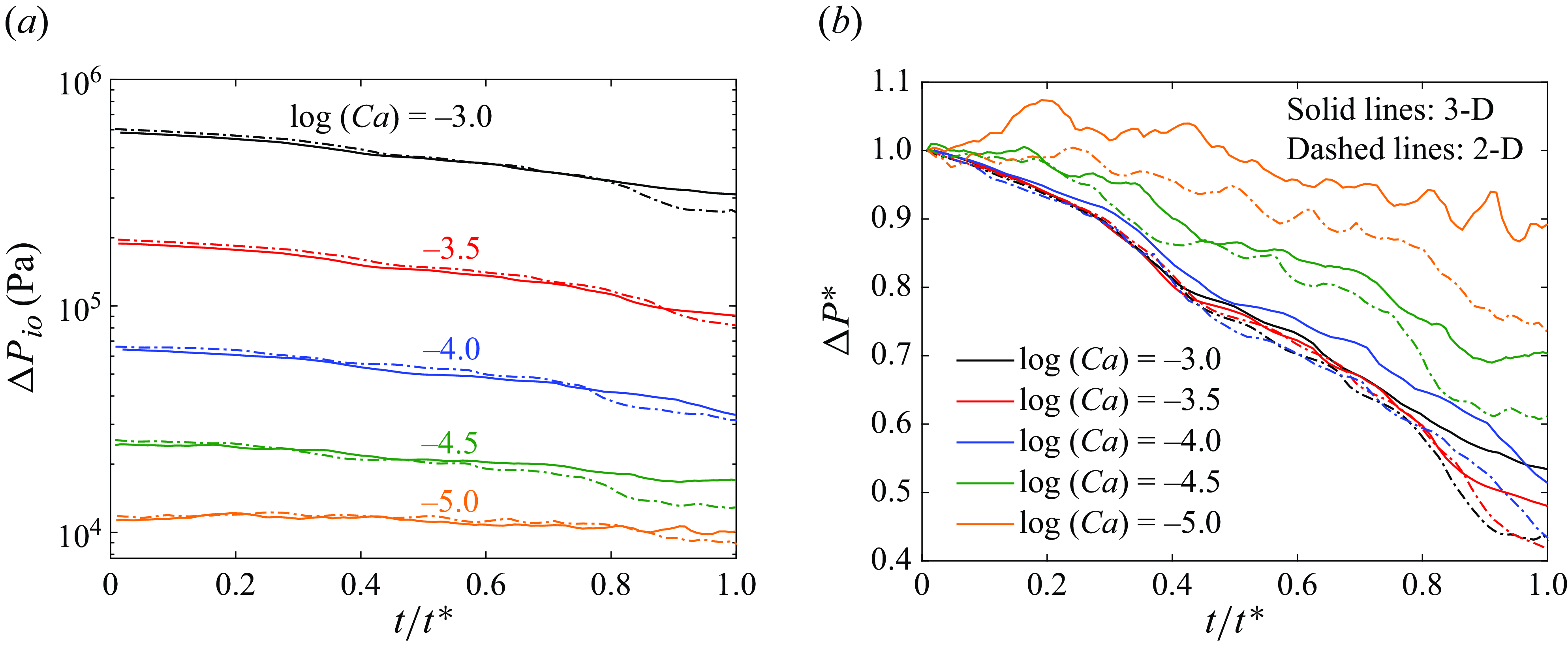
Figure 14. (a) Average pressure drop $\Delta P_{{io}}$
between the inlet and outlet of the fracture, as a function of time (normalised by the breakthrough time), for different
$\Delta P_{{io}}$
between the inlet and outlet of the fracture, as a function of time (normalised by the breakthrough time), for different $Ca$
values. (b) Normalised average pressure drop,
$Ca$
values. (b) Normalised average pressure drop, $\Delta P^*$
(
$\Delta P^*$
( $=\Delta P_{{io}}/\Delta P_{{io}}(t=0)$
) as a function of time. The solid and dashed lines correspond to the 3-D and 2-D simulation results, respectively.
$=\Delta P_{{io}}/\Delta P_{{io}}(t=0)$
) as a function of time. The solid and dashed lines correspond to the 3-D and 2-D simulation results, respectively.

Figure 15. Evolution of the interface length $l$
with time (normalised by
$l$
with time (normalised by $t^*$
) for three representative
$t^*$
) for three representative $Ca$
values. The solid and dashed curves represent the 3-D and 2-D results, respectively.
$Ca$
values. The solid and dashed curves represent the 3-D and 2-D results, respectively.
Fluid–fluid interface length: figure 15 presents the fluid–fluid interface lengths ( $l$
) within the mean aperture plane (
$l$
) within the mean aperture plane ( $xy$
) of the fracture as a function of the normalised time (
$xy$
) of the fracture as a function of the normalised time ( $t/t^*$
), for three representative capillary numbers. Across all
$t/t^*$
), for three representative capillary numbers. Across all $Ca$
values,
$Ca$
values, $l$
increases monotonically, and the growth is approximately linear with time. At higher
$l$
increases monotonically, and the growth is approximately linear with time. At higher $Ca$
, more pronounced viscous fingering results in larger interface lengths. Conversely, at lower
$Ca$
, more pronounced viscous fingering results in larger interface lengths. Conversely, at lower $Ca$
, the fingers become more compact, leading to shorter interface lengths. These trends are consistent with previous findings, both in rough fractures (Chen et al. Reference Chen, Guo, Wu and Hu2018) and in 2-D porous media (Ferrari et al. Reference Ferrari, Jimenez‐Martinez, Borgne, Méheust and Lunati2015). The 2-D and 3-D results for
$Ca$
, the fingers become more compact, leading to shorter interface lengths. These trends are consistent with previous findings, both in rough fractures (Chen et al. Reference Chen, Guo, Wu and Hu2018) and in 2-D porous media (Ferrari et al. Reference Ferrari, Jimenez‐Martinez, Borgne, Méheust and Lunati2015). The 2-D and 3-D results for $l$
show good agreement at lower
$l$
show good agreement at lower $Ca$
, where the influence of the wetting film is minimal. However, at larger
$Ca$
, where the influence of the wetting film is minimal. However, at larger $Ca$
discrepancies are more noticeable, due to more sustained secondary fingering in the 3-D simulations than in the 2-D model (figure 15
a
$Ca$
discrepancies are more noticeable, due to more sustained secondary fingering in the 3-D simulations than in the 2-D model (figure 15
a $^{\prime \prime }$
, 15
b
$^{\prime \prime }$
, 15
b $^{\prime \prime }$
). Furthermore, in large
$^{\prime \prime }$
). Furthermore, in large $Ca$
flows, break-up events, which occur significantly during the invasion process, further contribute to a steeper increase of
$Ca$
flows, break-up events, which occur significantly during the invasion process, further contribute to a steeper increase of $l$
in time (Pak et al. Reference Pak, Butler, Geiger, van Dijke and Sorbie2015; Chen et al. Reference Chen, Guo, Wu and Hu2018), a phenomenon that is captured by the 2-D model, although to a lesser extent. For further illustration of this behaviour, see the supplementary movies 1 (for three dimensions) and 2 (for two dimensions).
$l$
in time (Pak et al. Reference Pak, Butler, Geiger, van Dijke and Sorbie2015; Chen et al. Reference Chen, Guo, Wu and Hu2018), a phenomenon that is captured by the 2-D model, although to a lesser extent. For further illustration of this behaviour, see the supplementary movies 1 (for three dimensions) and 2 (for two dimensions).
Velocity of the most advanced finger’s tip: figure 16(a) shows the velocity of the tip, $U_{{tip}}$
, normalised by its mean value and denoted as
$U_{{tip}}$
, normalised by its mean value and denoted as $U^*_{{tip}}$
, as a function of the normalised time (
$U^*_{{tip}}$
, as a function of the normalised time ( $t/t^*$
).
$t/t^*$
). $U_{{tip}}$
is defined as the velocity at the point farthest from the inlet reached by the fluid–fluid interfaces. For clarity we have only shown the
$U_{{tip}}$
is defined as the velocity at the point farthest from the inlet reached by the fluid–fluid interfaces. For clarity we have only shown the $U^*_{{tip}}$
values for three representative
$U^*_{{tip}}$
values for three representative $Ca$
cases. The tip velocities fluctuate in time around their mean values, which increase linearly with
$Ca$
cases. The tip velocities fluctuate in time around their mean values, which increase linearly with $Ca$
; see inset of figure 16(b). At low
$Ca$
; see inset of figure 16(b). At low $Ca$
values (
$Ca$
values ( $\log ({Ca})=-4.5, -5.0$
), due to the magnitude of capillary forces with respect to viscous forces, the tip velocities show strong fluctuations. Their standard deviations are plotted as a function of
$\log ({Ca})=-4.5, -5.0$
), due to the magnitude of capillary forces with respect to viscous forces, the tip velocities show strong fluctuations. Their standard deviations are plotted as a function of $Ca$
in figure 16(b). While these fluctuations are well captured by the 2-D model at higher
$Ca$
in figure 16(b). While these fluctuations are well captured by the 2-D model at higher $Ca$
(
$Ca$
( $\log (Ca)\geqslant -4.0$
), they are relatively dampened for the two lowest
$\log (Ca)\geqslant -4.0$
), they are relatively dampened for the two lowest $Ca$
cases.
$Ca$
cases.
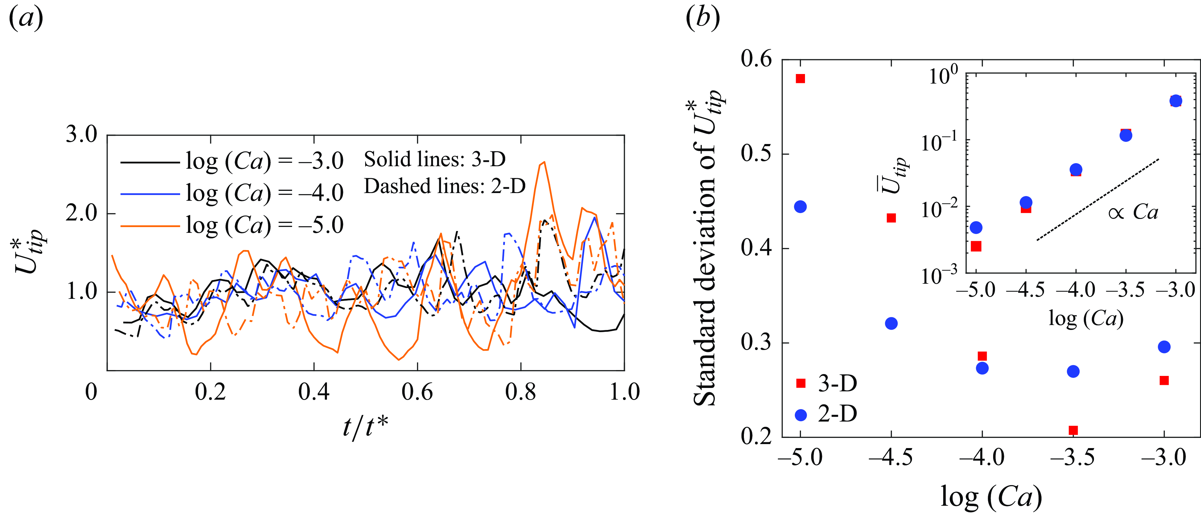
Figure 16. (a) Plot of velocity off the most advanced fluid–fluid interface tip, normalised by its mean value, $U^*_{{tip}} = U_{{tip}}/\overline {U}_{{tip}}$
with time (normalised by
$U^*_{{tip}} = U_{{tip}}/\overline {U}_{{tip}}$
with time (normalised by $t^*$
) for three representative
$t^*$
) for three representative $Ca$
values. The solid and dashed curves represent the 3-D and 2-D results, respectively. The standard deviations of
$Ca$
values. The solid and dashed curves represent the 3-D and 2-D results, respectively. The standard deviations of $U^*_{{tip}}$
values are plotted in (b) for all the investigated
$U^*_{{tip}}$
values are plotted in (b) for all the investigated $Ca$
values. Inset: plot of
$Ca$
values. Inset: plot of $\overline {U}_{{tip}}$
as a function of
$\overline {U}_{{tip}}$
as a function of $Ca$
values. The dashed line represents a reference with a slope of
$Ca$
values. The dashed line represents a reference with a slope of $1$
, indicating a linear scaling between
$1$
, indicating a linear scaling between $\overline {U}_{{tip}}$
and
$\overline {U}_{{tip}}$
and $Ca$
.
$Ca$
.
Longitudinal saturation profiles: we now examine the longitudinal saturation profile of the invading fluid, averaged in the transverse ( $y$
) direction (Ferrari et al. Reference Ferrari, Jimenez‐Martinez, Borgne, Méheust and Lunati2015). This profile is closely linked to the conventional macroscopic description of flow through permeable media, which relies on volume averaging (see, e.g. Bear Reference Bear2013). Figure 17 presents the mean saturation profile as a function of the normalised longitudinal coordinate
$y$
) direction (Ferrari et al. Reference Ferrari, Jimenez‐Martinez, Borgne, Méheust and Lunati2015). This profile is closely linked to the conventional macroscopic description of flow through permeable media, which relies on volume averaging (see, e.g. Bear Reference Bear2013). Figure 17 presents the mean saturation profile as a function of the normalised longitudinal coordinate $x/L_x$
, for three representative
$x/L_x$
, for three representative $Ca$
values. Overall, there is good agreement between the saturation profiles predicted by the 2-D and 3-D models at all capillary numbers. The discrepancies are small but appear larger at both ends of the
$Ca$
values. Overall, there is good agreement between the saturation profiles predicted by the 2-D and 3-D models at all capillary numbers. The discrepancies are small but appear larger at both ends of the $Ca$
range. At larger
$Ca$
range. At larger $Ca$
, the differences arise primarily because the wetting fluid film is not accounted for, as discussed above for other observables. At lower
$Ca$
, the differences arise primarily because the wetting fluid film is not accounted for, as discussed above for other observables. At lower $Ca$
, although the wetting film is thinner, small-scale variations in the invasion patterns lead to slightly larger mismatches in the profiles than at intermediate capillary numbers without a systematic pattern.
$Ca$
, although the wetting film is thinner, small-scale variations in the invasion patterns lead to slightly larger mismatches in the profiles than at intermediate capillary numbers without a systematic pattern.
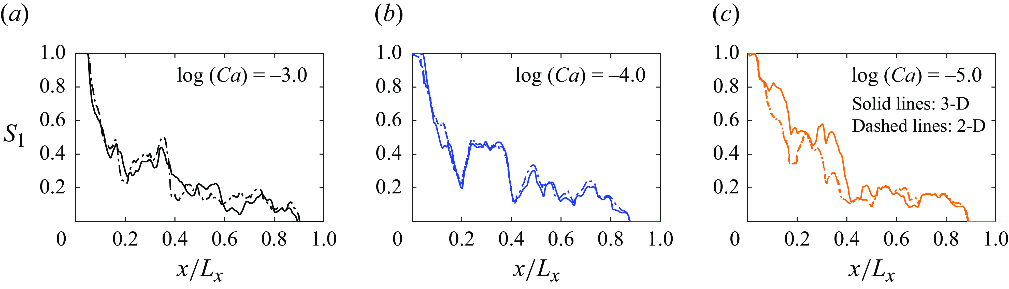
Figure 17. Average longitudinal saturation profile for three different, representative $Ca$
values. The solid and the dashed lines correspond to the 3-D and 2-D profiles respectively.
$Ca$
values. The solid and the dashed lines correspond to the 3-D and 2-D profiles respectively.
4.3.4. Discussion on the validity of the 2-D model’s assumptions
The derivation of the 2-D depth-integrated two-phase flow model relies on two key approximations: (i) the out-of-plane curvature approximation (3.29), and (ii) the estimate of the wall shear stress based on the assumption of a parabolic vertical velocity profile (3.17). Here, we assess the validity of these approximations.
Out-of-plane curvature approximation: to assess the accuracy of the out-of-plane curvature approximation in (3.29), we analyse the curvature of a 3-D interface obtained from the 3-D simulation results. The interface curvature $\kappa$
in the 3-D model can be decomposed in two components: the in-plane curvature
$\kappa$
in the 3-D model can be decomposed in two components: the in-plane curvature $\kappa _{{xy}}$
and the out-of-plane curvature
$\kappa _{{xy}}$
and the out-of-plane curvature $\kappa _{{z}}$
; this decomposition is used in the 2D-model, but in the 3-D model the total curvature
$\kappa _{{z}}$
; this decomposition is used in the 2D-model, but in the 3-D model the total curvature $\kappa$
is obtained directly from the divergence of the normalised gradient of the 3-D phase indicator function
$\kappa$
is obtained directly from the divergence of the normalised gradient of the 3-D phase indicator function $\gamma$
(2.7). On the one hand, we extract the
$\gamma$
(2.7). On the one hand, we extract the $\kappa$
values along the line defined as the intersection of the horizontal mid-plane of the fracture and the 3-D fluid–fluid interface. On the other hand, we compute, along the same line, the in-plane curvature
$\kappa$
values along the line defined as the intersection of the horizontal mid-plane of the fracture and the 3-D fluid–fluid interface. On the other hand, we compute, along the same line, the in-plane curvature $\kappa _{{xy}}$
, based on the divergence of the normalised gradient of the 2-D phase indicator function. Adding to this
$\kappa _{{xy}}$
, based on the divergence of the normalised gradient of the 2-D phase indicator function. Adding to this $\kappa _{{xy}}$
our analytical approximation for the out-of-plane contribution, given by
$\kappa _{{xy}}$
our analytical approximation for the out-of-plane contribution, given by $2/a \cos \theta$
, we thus reconstruct an estimate of the curvature of the 3-D fluid–fluid interface as
$2/a \cos \theta$
, we thus reconstruct an estimate of the curvature of the 3-D fluid–fluid interface as $\kappa _{{xy}} + (2/a) \cos \theta$
(
$\kappa _{{xy}} + (2/a) \cos \theta$
( $a$
being the local fracture aperture), which is exactly the curvature estimated by the 2-D depth-integrated model. For all voxels along the aforementioned fluid–fluid line in the fracture mid-plane, we then compare those two estimates of the 3-D interface’s curvature: the one calculated as the 3-D model would, and the one estimated as the 2-D model would. The results are shown in figure 18(d–f) for three representative capillary numbers:
$a$
being the local fracture aperture), which is exactly the curvature estimated by the 2-D depth-integrated model. For all voxels along the aforementioned fluid–fluid line in the fracture mid-plane, we then compare those two estimates of the 3-D interface’s curvature: the one calculated as the 3-D model would, and the one estimated as the 2-D model would. The results are shown in figure 18(d–f) for three representative capillary numbers: $\log (Ca) = -3.0, -4.0$
and
$\log (Ca) = -3.0, -4.0$
and $-5.0$
; we use an occupancy density plot rather than a scatter plot, which would not show the spatial repartition of the points in the plane of the figure as well. The mid-plane fluid–fluid lines corresponding to each of these plots are shown in figure 18(a−c). Figure 18(d–f) very clearly indicate that while the curvature inferred by the 2-D depth-integrated model slightly underpredicts that computed by the 3-D model, the agreement between the two values varies from good to excellent over the investigated range of capillary numbers, the best agreement being obtained at the largest capillary number (
$-5.0$
; we use an occupancy density plot rather than a scatter plot, which would not show the spatial repartition of the points in the plane of the figure as well. The mid-plane fluid–fluid lines corresponding to each of these plots are shown in figure 18(a−c). Figure 18(d–f) very clearly indicate that while the curvature inferred by the 2-D depth-integrated model slightly underpredicts that computed by the 3-D model, the agreement between the two values varies from good to excellent over the investigated range of capillary numbers, the best agreement being obtained at the largest capillary number ( $\log (Ca) = -3.0$
). The larger discrepancies observed at lower capillary numbers are likely due to stronger curvatures at localised positions along the fluid–fluid line, which cause increased variations in the out-of-plane curvature component. Nevertheless, the overall agreement between the two estimates supports the validity of the assumptions made to ‘reconstruct’ the full capillary force in the 2-D model without explicitly describing the third dimension, over the full range of investigated capillary numbers.
$\log (Ca) = -3.0$
). The larger discrepancies observed at lower capillary numbers are likely due to stronger curvatures at localised positions along the fluid–fluid line, which cause increased variations in the out-of-plane curvature component. Nevertheless, the overall agreement between the two estimates supports the validity of the assumptions made to ‘reconstruct’ the full capillary force in the 2-D model without explicitly describing the third dimension, over the full range of investigated capillary numbers.
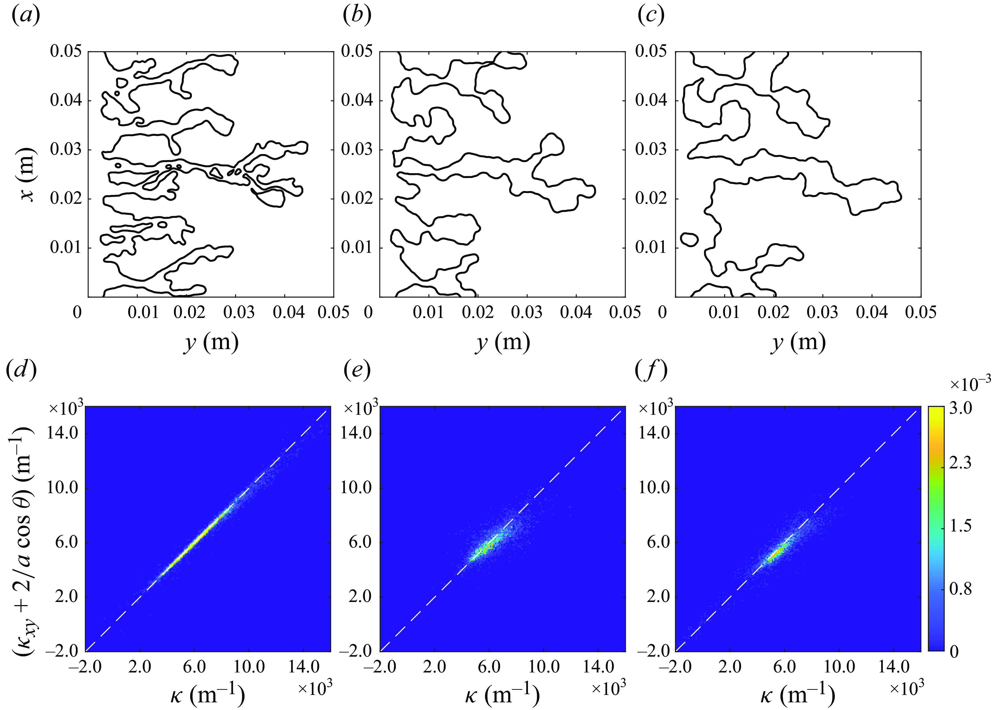
Figure 18. (a−c) Interface morphologies obtained as intersections between the horizontal mid-plane of the fracture and fluid–fluid interfaces obtained with the 3-D model, for three representative capillary numbers: $\log (Ca) = -3.0, -4.0$
and
$\log (Ca) = -3.0, -4.0$
and $-5.0$
. (d−f) Comparison between the curvature
$-5.0$
. (d−f) Comparison between the curvature $\kappa$
calculated from the 3-D interface geometry through (2.7) and that estimated by the 2-D model from the sole knowledge of the corresponding 2-D pattern shown above, as
$\kappa$
calculated from the 3-D interface geometry through (2.7) and that estimated by the 2-D model from the sole knowledge of the corresponding 2-D pattern shown above, as $\kappa _{{xy}} + 2/a \cos \theta$
, where
$\kappa _{{xy}} + 2/a \cos \theta$
, where $\kappa _{{xy}}$
is measured from the 2-D pattern; the comparison is performed through occupation density maps. The dashed diagonal line represents the ideal agreement.
$\kappa _{{xy}}$
is measured from the 2-D pattern; the comparison is performed through occupation density maps. The dashed diagonal line represents the ideal agreement.
Vertical velocity profiles: similarly to our analysis performed in the Hele-Shaw cell geometry (§ 4.2.2), we have tested the validity of our assumption of parabolic vertical velocity profile (3.17) by plotting in figure 19 the $z$
coordinate
$z$
coordinate $x$
at four given locations within the fracture plane, as a function of the
$x$
at four given locations within the fracture plane, as a function of the $x$
-component of the 3-D velocity, for the two extreme
$x$
-component of the 3-D velocity, for the two extreme $Ca$
values (
$Ca$
values ( $\log (Ca)=-3.0$
and
$\log (Ca)=-3.0$
and $-5.0$
). The horizontal coordinates of these locations are such that they lie sufficiently away from the fluid-fluid interface, in areas occupied by either of the two fluids, 1 and 2. It can be observed that, for both
$-5.0$
). The horizontal coordinates of these locations are such that they lie sufficiently away from the fluid-fluid interface, in areas occupied by either of the two fluids, 1 and 2. It can be observed that, for both $Ca$
cases, the profiles are perfectly parabolic at the locations occupied by the defending fluid only, (figures 19
b and 19
d). For the locations occupied by the invading fluid, the velocity profile fits a parabolic representation (in the vertical range corresponding to the invading fluid, that is, excluding the film of defending fluid at the walls) only at low
$Ca$
cases, the profiles are perfectly parabolic at the locations occupied by the defending fluid only, (figures 19
b and 19
d). For the locations occupied by the invading fluid, the velocity profile fits a parabolic representation (in the vertical range corresponding to the invading fluid, that is, excluding the film of defending fluid at the walls) only at low $Ca$
(low
$Ca$
(low $Re$
case; figure 19
c). At the highest
$Re$
case; figure 19
c). At the highest $Ca$
(
$Ca$
( $Re=0.324$
), a relatively thicker film and possibly also increased inertial effects (though moderate), influence the velocity profile, which considerably deviates from being parabolic, as seen in figure 19(a). However, one can infer from these plots that as long as Stokes flow (
$Re=0.324$
), a relatively thicker film and possibly also increased inertial effects (though moderate), influence the velocity profile, which considerably deviates from being parabolic, as seen in figure 19(a). However, one can infer from these plots that as long as Stokes flow ( $Re \ll 1$
) is maintained, one can expect local vertical velocity profiles in both fluids to be very close to parabolic.
$Re \ll 1$
) is maintained, one can expect local vertical velocity profiles in both fluids to be very close to parabolic.

Figure 19. Vertical profiles of the longitudinal component ( $x$
component) of the 3-D velocity, plotted at locations occupied by fluid 1 (a,c) and fluid 2 (b,d) and located sufficiently away from the interface. Panels (a,b) correspond to a snapshot at
$x$
component) of the 3-D velocity, plotted at locations occupied by fluid 1 (a,c) and fluid 2 (b,d) and located sufficiently away from the interface. Panels (a,b) correspond to a snapshot at $t = 0.055$
(
$t = 0.055$
( $t/t^*=0.44$
), obtained for the following flow conditions:
$t/t^*=0.44$
), obtained for the following flow conditions: $u_{{in}} = 100$
mm s−1,
$u_{{in}} = 100$
mm s−1, $\log (Ca) = -3.0$
,
$\log (Ca) = -3.0$
, $Re = 0.324$
, while panels (c,d) correspond to a snapshot obtained at
$Re = 0.324$
, while panels (c,d) correspond to a snapshot obtained at $t = 6.72$
s (
$t = 6.72$
s ( $t/t^*=0.43$
) for the following flow conditions:
$t/t^*=0.43$
) for the following flow conditions: $u_{{in}} = 1$
mm s–1,
$u_{{in}} = 1$
mm s–1, $\log (Ca) = -5.0$
,
$\log (Ca) = -5.0$
, $Re = 0.00324$
. The simulated profiles are shown by black circles, while the black dotted curves represent the corresponding best-fit parabolic profiles.
$Re = 0.00324$
. The simulated profiles are shown by black circles, while the black dotted curves represent the corresponding best-fit parabolic profiles.
4.3.5. Remarks on the computational efficiency of the 2-D integrated model
The analysis in the previous sections demonstrates that the 2-D depth-averaged model with effective terms capturing the effects of the third dimension captures the essential physics of immiscible flow in rough fractures, at least for drainage for which no wall film flow of the displacing fluid is to be expected, and accurately predicts both hydrodynamic-scale and mesoscopic to macroscopic flow observables. To assess its computational efficiency for the numerical simulations across different geometries, the computational requirements of the 3-D and the 2-D models are presented in table 4. The 2-D model achieves a substantial reduction in the total cell count, typically by at least one order of magnitude, compared with the 3-D grid. Furthermore, constrained by the CFL stability criterion, the computational effort is also influenced by the number of time steps and the time-step size. The 3-D model, with its finer grid resolution, necessitates smaller time steps due to the CFL criterion, contributing to increased computational effort. Our simulations consistently indicate that the time steps in the 2-D model are approximately one order of magnitude larger than those required by the 3-D model. The advantage of coarser grid resolution and higher time-step size is reflected in the total CPU hours required by the 2-D model simulations, as highlighted in table 4. On average, 2-D model simulations utilise 5−10 times less CPU time than their 3-D counterparts.
Table 4. Grid sizes and total CPU hours required by the 3-D and the 2-D model computations, for the Hele-Shaw cell and the rough fracture geometry. The grid cell counts are shown as $n_x\times n_y\times n_z$
, where
$n_x\times n_y\times n_z$
, where $n_x$
,
$n_x$
, $n_y$
and
$n_y$
and $n_z$
are the number of cells in the
$n_z$
are the number of cells in the $x$
,
$x$
, $y$
and
$y$
and $z$
directions, respectively. The presented values correspond to the extreme investigated
$z$
directions, respectively. The presented values correspond to the extreme investigated $Ca$
flow cases for the two considered geometries. All simulations were conducted in parallel on the cluster system at the Leibniz University of Hannover, Germany.
$Ca$
flow cases for the two considered geometries. All simulations were conducted in parallel on the cluster system at the Leibniz University of Hannover, Germany.
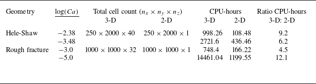
When it comes to the investigated range of capillary numbers $[10^{-5}; 10^{-3}]$
, it is relevant for such VOF-based DNS of two-phase flow (see, e.g. Krishna et al. Reference Krishna, Méheust and Neuweiler2024). Indeed, such VOF direct numerical simulations (even in three dimensions) are difficult to run at very low capillary numbers due to the numerical errors known as spurious currents (parasitic velocities) (Lafaurie et al. Reference Lafaurie, Nardone, Scardovelli, Zaleski and Zanetti1994; Deshpande et al. Reference Deshpande, Anumolu and Trujillo2012b
; Popinet Reference Popinet2018). At very low capillary numbers, an invasion percolation scheme is sufficient and runs very fast (Yang et al. Reference Yang, Neuweiler, Méheust, Fagerlund and Niemi2016), while at very large capillary numbers direct numerical simulations run very inefficiently (see an alternative, much more efficient numerical approach in Yang et al. (Reference Yang, Méheust, Neuweiler, Hu, Niemi and Chen2019)). In addition, many practical subsurface applications, such as CO
$[10^{-5}; 10^{-3}]$
, it is relevant for such VOF-based DNS of two-phase flow (see, e.g. Krishna et al. Reference Krishna, Méheust and Neuweiler2024). Indeed, such VOF direct numerical simulations (even in three dimensions) are difficult to run at very low capillary numbers due to the numerical errors known as spurious currents (parasitic velocities) (Lafaurie et al. Reference Lafaurie, Nardone, Scardovelli, Zaleski and Zanetti1994; Deshpande et al. Reference Deshpande, Anumolu and Trujillo2012b
; Popinet Reference Popinet2018). At very low capillary numbers, an invasion percolation scheme is sufficient and runs very fast (Yang et al. Reference Yang, Neuweiler, Méheust, Fagerlund and Niemi2016), while at very large capillary numbers direct numerical simulations run very inefficiently (see an alternative, much more efficient numerical approach in Yang et al. (Reference Yang, Méheust, Neuweiler, Hu, Niemi and Chen2019)). In addition, many practical subsurface applications, such as CO $_2$
sequestration (Krevor et al. Reference Krevor, Blunt, Benson, Pentland, Reynolds, Al-Menhali and Niu2015), often operate in this intermediate-to-high Ca range.
$_2$
sequestration (Krevor et al. Reference Krevor, Blunt, Benson, Pentland, Reynolds, Al-Menhali and Niu2015), often operate in this intermediate-to-high Ca range.
5. Summary and conclusions
In this paper, we have proposed a novel two-dimensional depth-integrated model describing immiscible two-phase flows in open rough-walled fractures. Such models of reduced dimensionality can be beneficial if predictions of two-phase flow in fractures need to be made over larger length scales. The 2-D model was derived using a DNS approach employing the VOF method to resolve the fluid–fluid interface. By assuming a sufficiently small aperture gradients (i.e. the lubrication approximation) and a parabolic transverse velocity profile, the governing equations were integrated over the direction perpendicular to the fracture’s mean plane, resulting in a 2-D representation of the flow field in terms of depth-averaged quantities. The primary variables in the model are the local flux (i.e. depth-integrated fluid velocity) and fluid pressure, while the fracture’s geometric description can be reduced to its aperture field and mean topography field (i.e. the average between the rough topographies of the two fracture walls). If the two fluids have the same density, the sole aperture field controls the displacement process. The wall friction and out-of-plane curvature component of the fluid–fluid interface are accounted for by corresponding terms and parameters in the 2-D model equations that were derived in the averaging procedure. Additionally, the transport equation of the fluid indicator function of the 2-D model contains a storage prefactor in its non-stationary term.
We tested the 2-D model using the classical viscous finger growth in a Hele-Shaw geometry. The finger width and pressure drops could well be reproduced for larger capillary numbers, while the width was slightly underpredicted at lower capillary numbers, where local 3-D configurations of the fluid–fluid interface impact the overall finger shape. Subsequently, the model was applied to viscously unstable drainage in a synthetic rough fracture whose wall topographies and aperture field resemble those of a naturally occurring geological fracture, and whose distribution of aperture gradients is actually typical of what could be measured on real geological fractures, and significantly wider than strictly required by the lubrication approximation. The wall roughness and the resulting spatial heterogeneity of the aperture field bring an additional physical feature to the two-phase flow process, as fluid patterns are not entirely controlled by the viscous instability, but also strongly impacted by the geometry of the aperture field. The drainage simulations covered a broad range of capillary numbers ( $10^{-5} \leqslant Ca \leqslant 10^{-3}$
), for which the use of such VOF-based DNS is relevant, and compared the 2-D depth-integrated model’s predictions with the 3-D numerical model results. Our comparison demonstrated that the 2-D model effectively captures the relevant flow physics of the drainage process. This means that the fluid displacement morphology and macroscopic observables (e.g. macroscopic pressure drop and longitudinal saturation profiles) as well as the transition from viscous-dominated to capillary-dominated displacement regimes, as characterised by the pressure signals, was well reproduced. Effects where films are relevant, such as rupturing or bursts, which at few places occurred at high capillary numbers, as well as some small-scale details at low capillary numbers, were less markedly captured. The displacement patterns from the fracture scale and down to
$10^{-5} \leqslant Ca \leqslant 10^{-3}$
), for which the use of such VOF-based DNS is relevant, and compared the 2-D depth-integrated model’s predictions with the 3-D numerical model results. Our comparison demonstrated that the 2-D model effectively captures the relevant flow physics of the drainage process. This means that the fluid displacement morphology and macroscopic observables (e.g. macroscopic pressure drop and longitudinal saturation profiles) as well as the transition from viscous-dominated to capillary-dominated displacement regimes, as characterised by the pressure signals, was well reproduced. Effects where films are relevant, such as rupturing or bursts, which at few places occurred at high capillary numbers, as well as some small-scale details at low capillary numbers, were less markedly captured. The displacement patterns from the fracture scale and down to $L_{{c}}/10$
, as well as macroscopic observables, however, were captured well over the entire capillary number range. Discrepancies arise at larger
$L_{{c}}/10$
, as well as macroscopic observables, however, were captured well over the entire capillary number range. Discrepancies arise at larger $Ca$
values since wetting films, which are resolved by the 3-D model but not in the 2-D model, have a larger thickness that grows with the capillary number. The 2-D model at higher
$Ca$
values since wetting films, which are resolved by the 3-D model but not in the 2-D model, have a larger thickness that grows with the capillary number. The 2-D model at higher $Ca$
values thus features slower finger velocities, and slightly different fingering patterns at large scales, as the presence of the film reduces the effective mean aperture in the 3-D model and modifies the related boundary conditions for the injected fluid, from no flow to slip velocity. In contrast, at lower
$Ca$
values thus features slower finger velocities, and slightly different fingering patterns at large scales, as the presence of the film reduces the effective mean aperture in the 3-D model and modifies the related boundary conditions for the injected fluid, from no flow to slip velocity. In contrast, at lower $Ca$
values, the discrepancies in the patterns are primarily of smaller scales due to the strong local aperture variations, where the assumption of mild aperture gradients no longer applies, and the sensitivity of the fingering process to local aperture fluctuations due to the dominant role by capillary effects. The best agreements between the 2-D and the 3-D model results are seen in the intermediate
$Ca$
values, the discrepancies in the patterns are primarily of smaller scales due to the strong local aperture variations, where the assumption of mild aperture gradients no longer applies, and the sensitivity of the fingering process to local aperture fluctuations due to the dominant role by capillary effects. The best agreements between the 2-D and the 3-D model results are seen in the intermediate $Ca$
range, where both the film effects and the capillary forces are not too large.
$Ca$
range, where both the film effects and the capillary forces are not too large.
While our analysis has been primarily focused on drainage simulations, it is anticipated that our 2-D depth-integrated model will perform well under imbibition conditions in the regimes for which film flow does not substantially influence the invasion patterns. With its capacity to offer a tenfold reduction in computational requirements in comparison with the 3-D numerical simulation, and reasonably accurate predictions over several decades in $Ca$
, we believe that this model will allow simulating a sufficiently large statistics of realisations of fracture with the same given set of geometrical parameters to tackle stochastic studies of two-phase flows in rough fractures. Note, however, that care has to be taken when studying phenomena for which deterministic small-scale details of the interface morphology matter. For instance, the interfacial area is crucial when studying effective rates of chemical reactions between the two fluids or the dissolution of components from one fluid into the other one. Phenomena that depend on the 3-D interface configuration, such as snap-off, are also expected to not be necessarily well captured by the 2-D model.
$Ca$
, we believe that this model will allow simulating a sufficiently large statistics of realisations of fracture with the same given set of geometrical parameters to tackle stochastic studies of two-phase flows in rough fractures. Note, however, that care has to be taken when studying phenomena for which deterministic small-scale details of the interface morphology matter. For instance, the interfacial area is crucial when studying effective rates of chemical reactions between the two fluids or the dissolution of components from one fluid into the other one. Phenomena that depend on the 3-D interface configuration, such as snap-off, are also expected to not be necessarily well captured by the 2-D model.
Investigation of such effects could warrant future studies. Other potential future prospects for this 2-D depth-integrated model include the characterisation of flow regimes over a wide range of capillary numbers and viscosity ratios, using a combination of 2-D simulations (when they are sufficiently accurate) and 3-D simulations (when they are necessary).
Supplementary movies
Supplementary movies. are available at https://doi.org/10.1017/jfm.2025.404.
Acknowledgements
This work was supported by the LUH compute cluster, funded by Leibniz Universität Hannover, the Lower Saxony Ministry of Science and Culture (MWK), and the German Research Foundation (DFG). We gratefully acknowledge the use of these computational resources for conducting the simulations.
Funding
This research was financially supported by the Deutsche Forschungsgemeinschaft (DFG, German Research Foundation) under project no. NE 824/20-1 and the Agence Nationale de la Recherche (ANR, French National Research Agency) under project no. ANR-20-CE92-0026 for the DFG-ANR project ‘2PhlowFrac’.
Declaration of interests
The authors report no conflict of interest.
Author contributions
R. Krishna: Data curation (lead); Formal analysis (equal); Investigation (lead); Methodology (equal); Software (lead); Validation (lead); Visualisation (lead); Writing – original draft (lead). Y. Méheust: Conceptualisation (equal); Data curation (supporting); Formal analysis (equal); Funding acquisition (equal); Investigation (supporting); Methodology (equal); Project administration (supporting); Resources (supporting); Software (supporting); Supervision (supporting); Validation (supporting); Visualisation (supporting); Writing – original draft (supporting); Writing – review & editing (equal). I. Neuweiler: Conceptualisation (equal); Data curation (supporting); Formal analysis (equal); Funding acquisition (equal); Investigation (supporting); Methodology (equal); Project administration (lead); Resources (lead); Software (Supporting); Supervision (lead); Validation (supporting); Visualisation (supporting); Writing – original draft (supporting); Writing – review & editing (equal).
Data availability statement
The data that support the findings of this study are available from the corresponding author upon reasonable request.
Appendix A. Particular case of a steady-state Stokes flow
In the case of a permanent flow at low Reynolds numbers, both momentum derivatives can be considered null, and thus the single-phase depth-integrated momentum conservation equation (3.19) reduces to
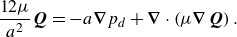 \begin{equation} \frac {12 \mu }{a^2} \boldsymbol{Q} = -a\boldsymbol{\nabla } p_{{d}} + \boldsymbol{\nabla }\cdot \left (\mu \boldsymbol{\nabla } \boldsymbol Q \right). \end{equation}
On account of the lubrication approximation ( $\mathcal{B}$
§ 3.1), the derivative of any velocity component with respect to
$\mathcal{B}$
§ 3.1), the derivative of any velocity component with respect to $z$
is much larger than the derivative with respect to
$z$
is much larger than the derivative with respect to $x$
and
$x$
and $y$
, and thus, the viscous force (Laplacian) term is expected to be much smaller than the wall friction (Darcian) term in the depth-integrated equation. Neglecting the former with respect to the latter, we obtain
$y$
, and thus, the viscous force (Laplacian) term is expected to be much smaller than the wall friction (Darcian) term in the depth-integrated equation. Neglecting the former with respect to the latter, we obtain
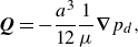 \begin{equation} \boldsymbol{Q} = -\frac {a^3}{12} \frac {1}{\mu } \boldsymbol{\nabla } p_{{d}}, \end{equation}
at any position in the mean fracture plane. This Darcy law is classically denoted as the local cubic law, since it states that the relationship between the depth-integrated specific flow and the dynamic pressure gradient in a parallel plate fracture also holds locally inside a fracture of spatially varying aperture (provided that $\| \boldsymbol{\nabla } a \ll 1\|$
) (Zimmerman & Yeo Reference Zimmerman and Yeo2000), by considering the local fracture transmissivity
$\| \boldsymbol{\nabla } a \ll 1\|$
) (Zimmerman & Yeo Reference Zimmerman and Yeo2000), by considering the local fracture transmissivity $a^3/12$
. Together with the continuity equation (3.18), it yields the Reynolds equation
$a^3/12$
. Together with the continuity equation (3.18), it yields the Reynolds equation
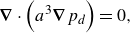 \begin{equation} \boldsymbol{\nabla } \cdot \left ( a^3 \boldsymbol{\nabla } p_{{d}} \right) = 0, \end{equation}
which can easily be solved to obtain the dynamic pressure field, and infer from it the $\boldsymbol Q$
and
$\boldsymbol Q$
and $\boldsymbol U$
fields. This method has been used to characterise flow channelling in rough geological fractures (Brown Reference Brown1987; Brown et al. Reference Brown, Stockman and Reeves1995; Méheust & Schmittbuhl Reference Méheust and Schmittbuhl2001).
$\boldsymbol U$
fields. This method has been used to characterise flow channelling in rough geological fractures (Brown Reference Brown1987; Brown et al. Reference Brown, Stockman and Reeves1995; Méheust & Schmittbuhl Reference Méheust and Schmittbuhl2001).
Appendix B. Effective contact angle and curvature analysis in 3-D Hele-Shaw configuration
As discussed in § 4.1, the out-of-plane curvature of the invading fluid–fluid interface increases in the presence of wetting films, which means that the effective contact angle $\theta _{{e}}$
to be used in the equation differs from the equilibrium contact angle
$\theta _{{e}}$
to be used in the equation differs from the equilibrium contact angle $\theta$
. In this appendix, we extend this discussion by analysing the curvature of the meniscus in the simplified case of a Hele-Shaw cell, based on film-resolved 3-D simulations.
$\theta$
. In this appendix, we extend this discussion by analysing the curvature of the meniscus in the simplified case of a Hele-Shaw cell, based on film-resolved 3-D simulations.
Figure 20 presents vertical cross-sections of the fluid–fluid interface in the longitudinal mid-plane of the flow cell (solid curves) for three capillary numbers, $-\log (Ca) = 2.38$
,
$-\log (Ca) = 2.38$
, $2.78$
and
$2.78$
and $3.48$
(ranging from high to low), as obtained from the 3-D simulations. Away from the finger tip and near the walls, the interface remains flat and parallel to the walls, leading to a uniform wetting-film thickness that decreases with decreasing
$3.48$
(ranging from high to low), as obtained from the 3-D simulations. Away from the finger tip and near the walls, the interface remains flat and parallel to the walls, leading to a uniform wetting-film thickness that decreases with decreasing $Ca$
. To determine the effective contact angle at the finger tip (the point of the interface farthest from the inlet), we first calculate the local out-of-plane interface curvature at that point. A circle (dotted) is then fitted to the tip with a radius
$Ca$
. To determine the effective contact angle at the finger tip (the point of the interface farthest from the inlet), we first calculate the local out-of-plane interface curvature at that point. A circle (dotted) is then fitted to the tip with a radius $r$
corresponding to the calculated curvature. These idealised circular meniscus radii, normalised by the cell aperture, are shown for the three
$r$
corresponding to the calculated curvature. These idealised circular meniscus radii, normalised by the cell aperture, are shown for the three $Ca$
cases in figure 20. Notably, even at the lowest
$Ca$
cases in figure 20. Notably, even at the lowest $Ca$
, where the wetting film is thinnest, the fitted circle does not intersect the cell walls, leading to an effective contact angle of
$Ca$
, where the wetting film is thinnest, the fitted circle does not intersect the cell walls, leading to an effective contact angle of $\theta _{{e}} = 180^\circ$
. While performing a similar analysis for simulations in the 3-D rough fracture geometries is challenging due to the geometric and dynamical complexities, the results from the Hele-Shaw cell provide a compelling argument for using an effective contact angle of
$\theta _{{e}} = 180^\circ$
. While performing a similar analysis for simulations in the 3-D rough fracture geometries is challenging due to the geometric and dynamical complexities, the results from the Hele-Shaw cell provide a compelling argument for using an effective contact angle of $180^\circ$
in the 2-D model across the capillary numbers investigated in this work. However, it is important to note that at extremely low capillary numbers, for which the wetting films become ultra-thin, the equilibrium contact angle values may suffice for the presented 2-D model.
$180^\circ$
in the 2-D model across the capillary numbers investigated in this work. However, it is important to note that at extremely low capillary numbers, for which the wetting films become ultra-thin, the equilibrium contact angle values may suffice for the presented 2-D model.
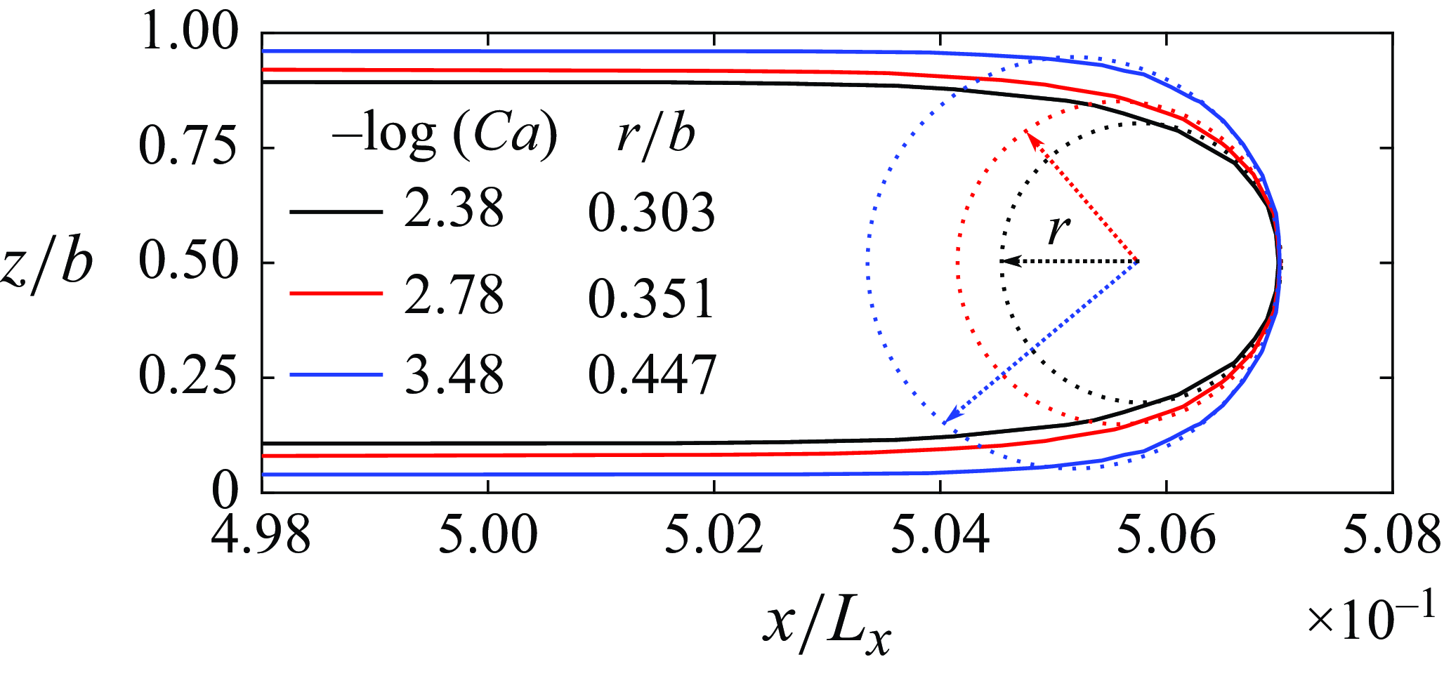
Figure 20. Direct 3-D numerical simulation of two-phase flow in a Hele-Shaw cell configuration, with proper resolution of the wall films in the vicinity of $z/b=\pm 0$
and
$z/b=\pm 0$
and $1$
: vertical cross-sections of the fluid–fluid interface in the longitudinal mid-plane for three different capillary numbers
$1$
: vertical cross-sections of the fluid–fluid interface in the longitudinal mid-plane for three different capillary numbers $Ca$
(
$Ca$
( $-\log (Ca) = 2.38$
,
$-\log (Ca) = 2.38$
, $2.78$
and
$2.78$
and $3.48$
), showing the variation of the meniscus curvature with
$3.48$
), showing the variation of the meniscus curvature with $Ca$
. The dashed circles are tangent to the interface at the displacement finger’s tip, so their normalised radii (
$Ca$
. The dashed circles are tangent to the interface at the displacement finger’s tip, so their normalised radii ( $r/b$
) correspond to the out-of-plane curvature radii of the interface at the corresponding finger tip. The measured film thicknesses at the centreline
$r/b$
) correspond to the out-of-plane curvature radii of the interface at the corresponding finger tip. The measured film thicknesses at the centreline $y=0$
are
$y=0$
are $42$
,
$42$
, $31$
and
$31$
and $15$
µm, respectively, for the aforementioned
$15$
µm, respectively, for the aforementioned $Ca$
values.
$Ca$
values.
Appendix C. Sensitivity of 2-D model predictions to the choice of the effective contact angle
In § 4.1 we discussed that, under drainage conditions, the presence of a uniform thin wetting film in the 3-D simulations, led us to choose an effective contact angle $\theta _{{a}}=180^\circ$
in the depth-integrated 2-D model (3.29). However, the reader might wonder how much this choice impacts the predicted displacement patterns. In this appendix, we thus test how changing the value of the effective contact angle impacts the 2-D model’s predictions as compared with our baseline case with
$\theta _{{a}}=180^\circ$
in the depth-integrated 2-D model (3.29). However, the reader might wonder how much this choice impacts the predicted displacement patterns. In this appendix, we thus test how changing the value of the effective contact angle impacts the 2-D model’s predictions as compared with our baseline case with $\theta _{{a}} = 180^\circ$
.
$\theta _{{a}} = 180^\circ$
.
For a capillary number such that $\log (Ca) = -4.0$
, the resulting invasion patterns are shown in figure 21 for two different effective contact angles, namely
$\log (Ca) = -4.0$
, the resulting invasion patterns are shown in figure 21 for two different effective contact angles, namely $\theta _{{a}} = 90^\circ$
(figure 21
$\theta _{{a}} = 90^\circ$
(figure 21 $(a-a^{\prime \prime })$
) and
$(a-a^{\prime \prime })$
) and $\theta _{{a}} = 135^\circ$
(figure 21
$\theta _{{a}} = 135^\circ$
(figure 21 $(b-b^{\prime \prime })$
). The resulting displacement patterns are shown superimposed with our baseline case of
$(b-b^{\prime \prime })$
). The resulting displacement patterns are shown superimposed with our baseline case of $\theta = 180^\circ$
. In the case of
$\theta = 180^\circ$
. In the case of $\theta = 90^\circ$
, the out-of-plane curvature contribution in (3.29), and hence the resulting capillary pressure component, vanish entirely. This effect is clearly observed in the resulting invasion patterns in figure 21
$\theta = 90^\circ$
, the out-of-plane curvature contribution in (3.29), and hence the resulting capillary pressure component, vanish entirely. This effect is clearly observed in the resulting invasion patterns in figure 21 $(a-a^{\prime \prime })$
, where smaller-scale details are comparatively smoothed out. To a lesser extent, this smoothing can also be observed in the case of
$(a-a^{\prime \prime })$
, where smaller-scale details are comparatively smoothed out. To a lesser extent, this smoothing can also be observed in the case of $\theta = 135^\circ$
(figure 21
$\theta = 135^\circ$
(figure 21 $(b-b^{\prime \prime })$
). To evaluate the contact angle’s influence on other flow quantities, we compared the invading fluid’s global saturation (
$(b-b^{\prime \prime })$
). To evaluate the contact angle’s influence on other flow quantities, we compared the invading fluid’s global saturation ( $S_1$
), interface length (
$S_1$
), interface length ( $l$
) and average pressure drop (
$l$
) and average pressure drop ( $\Delta P_{{io}}$
) at different instances. Relative to the baseline case of
$\Delta P_{{io}}$
) at different instances. Relative to the baseline case of $\theta = 180^\circ$
, the average relative differences in these observables were
$\theta = 180^\circ$
, the average relative differences in these observables were $21\, \%$
,
$21\, \%$
, $22\, \%$
, and
$22\, \%$
, and $8.5\, \%$
, respectively, for the
$8.5\, \%$
, respectively, for the $\theta = 90^\circ$
case, while for the
$\theta = 90^\circ$
case, while for the $\theta = 135^\circ$
case they were respectively
$\theta = 135^\circ$
case they were respectively $8\, \%$
,
$8\, \%$
, $9\, \%$
and
$9\, \%$
and $5\, \%$
. Similar observations are recorded for the
$5\, \%$
. Similar observations are recorded for the $Ca$
cases not shown here.
$Ca$
cases not shown here.

Figure 21. Comparison of invasion morphologies obtained using the 2-D model for two distinct effective contact angles, namely $(a-a^{\prime \prime })$ $\theta _{{e}}=90^\circ$
, and
$\theta _{{e}}=90^\circ$
, and $(b-b^{\prime \prime })$ $\theta _{{e}}=135^\circ$
, with that obtained for
$\theta _{{e}}=135^\circ$
, with that obtained for $\theta =180^\circ$
(baseline) used to carry out the 2-D numerical simulations presented above. The three columns depict the invasion patterns recorded at three different time steps. The capillary number is intermediate:
$\theta =180^\circ$
(baseline) used to carry out the 2-D numerical simulations presented above. The three columns depict the invasion patterns recorded at three different time steps. The capillary number is intermediate: $\log (Ca)=-4.0$
.
$\log (Ca)=-4.0$
.
Note, however, that experiments (and the 3-D model’s predictions) will only be sensitive to the contact angle if it prevents the development of a film of the defending wetting fluid on the fracture walls. This would occur for values of the wetting angle very close to 90°. For such cases, in order for the 2-D model to predict the drainage process well, it would have to be run with an effective contact angle $\theta _{{a}}=90$
°, while in configurations where a wall film is present (that is, in most cases), an effective contact angle of
$\theta _{{a}}=90$
°, while in configurations where a wall film is present (that is, in most cases), an effective contact angle of $\theta _{{a}}=180$
° must be chosen.
$\theta _{{a}}=180$
° must be chosen.
Appendix D. Influence of aperture field discretisation on predicted invasion patterns and flow quantities
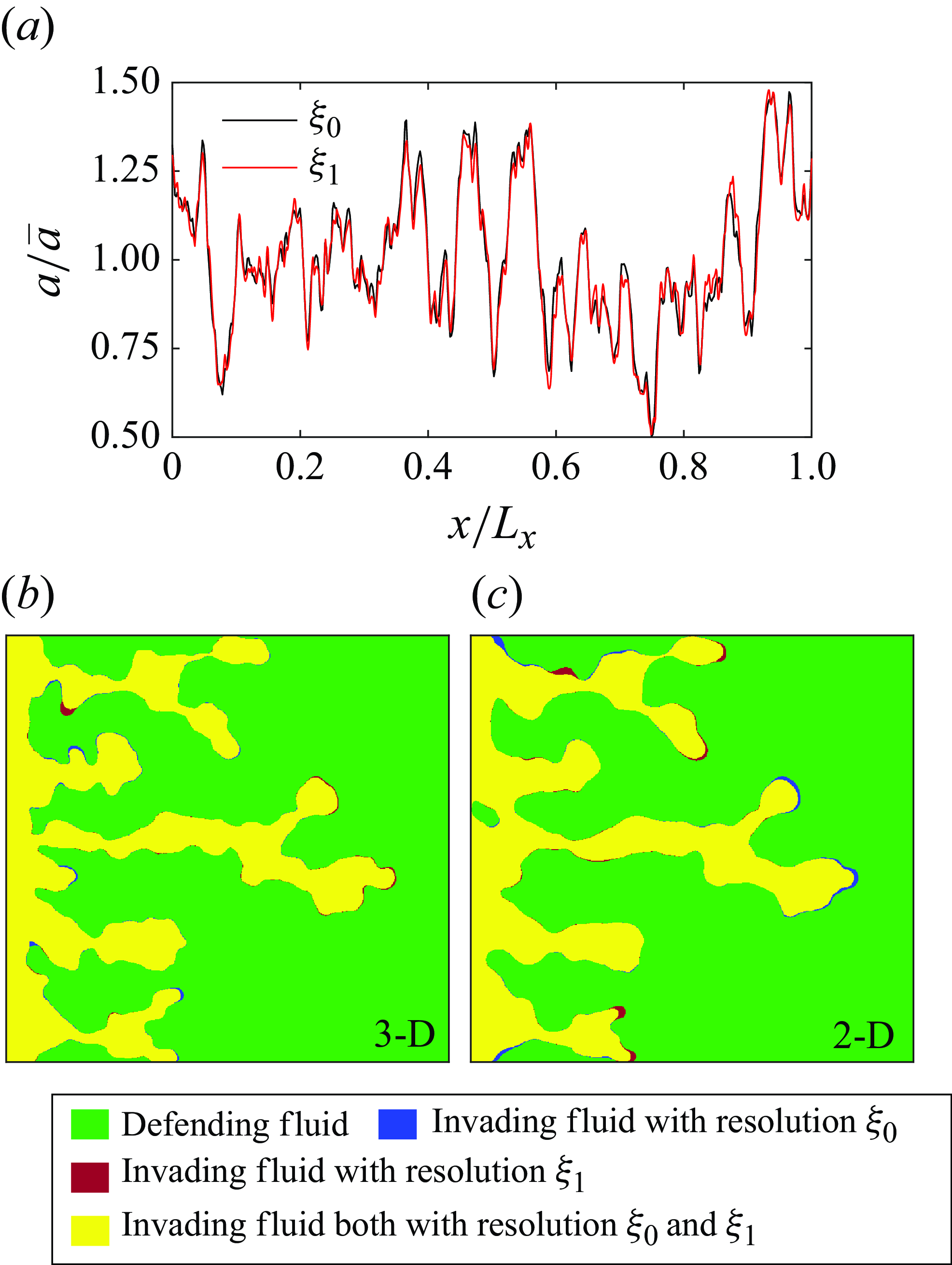
Figure 22. $(a)$
Aperture profile (normalised by the mean aperture
$(a)$
Aperture profile (normalised by the mean aperture $\bar {a}$
) along the longitudinal direction (
$\bar {a}$
) along the longitudinal direction ( $x$
) at the mid-line
$x$
) at the mid-line $y = L_y/2$
, obtained using the original aperture field resolution
$y = L_y/2$
, obtained using the original aperture field resolution $\xi _0$
(
$\xi _0$
( $512 \times 512$
) and a finer resolution
$512 \times 512$
) and a finer resolution $\xi _1$
(
$\xi _1$
( $1024 \times 1024$
). Panels
$1024 \times 1024$
). Panels $(b)$
and
$(b)$
and $(c)$
illustrate the comparison of the invasion patterns generated by the 3-D and 2-D models, respectively, for the two aperture field resolutions. The results correspond to the intermediate
$(c)$
illustrate the comparison of the invasion patterns generated by the 3-D and 2-D models, respectively, for the two aperture field resolutions. The results correspond to the intermediate $Ca$
case with
$Ca$
case with $\log (Ca) = -4.0$
.
$\log (Ca) = -4.0$
.
In this appendix we test the sensitivity of the predicted invasion patterns and various flow observables to a refinement of the aperture field discretisation. In all numerical presented above, the rough fracture geometry was generated on a $512 \times 512$
grid, corresponding to a horizontal resolution of
$512 \times 512$
grid, corresponding to a horizontal resolution of $\xi _0 = 97$
µm, while the computational mesh had a cell size of
$\xi _0 = 97$
µm, while the computational mesh had a cell size of $50$
µm. The
$50$
µm. The $512 \times 512$
discretisation of the aperture field was obtained from wall surface topographies that were sampled more finely, allowing us to also obtain a
$512 \times 512$
discretisation of the aperture field was obtained from wall surface topographies that were sampled more finely, allowing us to also obtain a $1024 \times 1024$
discretisation of the same aperture field, corresponding to a
$1024 \times 1024$
discretisation of the same aperture field, corresponding to a $\xi _1 = 48$
µm resolution. The same profile of the aperture field, i.e. intersection of that field with a vertical plane at
$\xi _1 = 48$
µm resolution. The same profile of the aperture field, i.e. intersection of that field with a vertical plane at $y = L_y/2$
, is shown in figure 22(a) for the two discretisations. The 3-D and 2-D numerical simulations were then re-run with the finer discretisation of the aperture field. Figures 22(b) and 22(c) show a comparison between the displacement patterns obtained for the aperture field resolutions
$y = L_y/2$
, is shown in figure 22(a) for the two discretisations. The 3-D and 2-D numerical simulations were then re-run with the finer discretisation of the aperture field. Figures 22(b) and 22(c) show a comparison between the displacement patterns obtained for the aperture field resolutions $\xi _0$
and
$\xi _0$
and $\xi _1$
, for a representative, intermediate capillary number case (
$\xi _1$
, for a representative, intermediate capillary number case ( $\log (Ca) = -4.0$
); panel (b) shows the result obtained from 3-D model, panel (c) those obtained from the 2-D model. The displacement patterns obtained with the two resolutions are mostly identical to each other, with minimal discrepancies. The corresponding macroscopic observables confirm this good agreement: the invading fluid saturation (
$\log (Ca) = -4.0$
); panel (b) shows the result obtained from 3-D model, panel (c) those obtained from the 2-D model. The displacement patterns obtained with the two resolutions are mostly identical to each other, with minimal discrepancies. The corresponding macroscopic observables confirm this good agreement: the invading fluid saturation ( $S_1$
), interface length (
$S_1$
), interface length ( $l$
) and average pressure drop (
$l$
) and average pressure drop ( $\Delta P_{{io}}$
) exhibit on average (over different times), relative differences of
$\Delta P_{{io}}$
) exhibit on average (over different times), relative differences of $0.008\, \%$
,
$0.008\, \%$
, $0.05\, \%$
and
$0.05\, \%$
and $0.9\, \%$
, respectively, for the 3-D model, while for the 2-D model these relative differences were respectively
$0.9\, \%$
, respectively, for the 3-D model, while for the 2-D model these relative differences were respectively $0.8\, \%$
,
$0.8\, \%$
, $0.5\, \%$
and
$0.5\, \%$
and $0.6\, \%$
. These findings suggest that the resolution
$0.6\, \%$
. These findings suggest that the resolution $\xi _0$
is sufficient to capture the essential physics of the immiscible displacement process, despite the fact the multiscale nature of the fracture walls’ geometry.
$\xi _0$
is sufficient to capture the essential physics of the immiscible displacement process, despite the fact the multiscale nature of the fracture walls’ geometry.
Appendix E. Single-phase 2-D depth-integrated model results
In this appendix, we present the results for the single-phase 2-D depth-integrated model, derived in § 3.2, and compare them with the full 3-D single-phase model results. The computational domain we choose for this comparison is the same as that used previously for the two-phase model results, detailed in figure 10. For the reference 3-D results, the single-phase governing equations (3.3) and (3.4) are solved numerically on a 3-D mesh (figure 11), while the 2-D depth-integrated single-phase equations (3.18) and (3.19) are solved on a 2-D mesh (similar to figure 3
b). The 3-D computational mesh used for these single-phase simulations is the same as that employed in the two-phase simulations in § 4.3.2, with additional refinement near the top and bottom walls. The 2-D computational mesh consists of only one cell in the $z$
direction, with no boundary conditions imposed on its top and bottom faces. The boundary conditions imposed on the different domain boundaries are the same for the 2-D and 3-D models, as shown in table 2, except for the phase-fraction
$z$
direction, with no boundary conditions imposed on its top and bottom faces. The boundary conditions imposed on the different domain boundaries are the same for the 2-D and 3-D models, as shown in table 2, except for the phase-fraction $\gamma$
, as a single fluid now occupies the entire computational domain. The fluid properties (invading fluid 1 used in the two-phase simulations) and flow conditions are listed in table 5. Here, we consider configurations of non-Stokes flow, with
$\gamma$
, as a single fluid now occupies the entire computational domain. The fluid properties (invading fluid 1 used in the two-phase simulations) and flow conditions are listed in table 5. Here, we consider configurations of non-Stokes flow, with $Re = 0.5$
,
$Re = 0.5$
, $5.0$
and,
$5.0$
and, $10$
. The resulting inlet velocities and Reynolds numbers are listed in table 5. In the case of the 2-D depth-integrated model, where the primary variable is the local flux
$10$
. The resulting inlet velocities and Reynolds numbers are listed in table 5. In the case of the 2-D depth-integrated model, where the primary variable is the local flux $\boldsymbol{Q} = (Q_x, Q_y)$
, the flow rate at the inlet boundary is prescribed as
$\boldsymbol{Q} = (Q_x, Q_y)$
, the flow rate at the inlet boundary is prescribed as $Q_{{in}}=u_{{in}}\:a(0,y),$
resulting in a spatially varying boundary condition. All simulations are run for a large number of time steps to obtain a steady-state solution. Note that, when comparing the velocity and local flux fields between the results from the 2-D and 3-D models, the notations used for the local flux and depth-averaged velocity fields obtained from the 2-D depth-averaged model are respectively
$Q_{{in}}=u_{{in}}\:a(0,y),$
resulting in a spatially varying boundary condition. All simulations are run for a large number of time steps to obtain a steady-state solution. Note that, when comparing the velocity and local flux fields between the results from the 2-D and 3-D models, the notations used for the local flux and depth-averaged velocity fields obtained from the 2-D depth-averaged model are respectively $\boldsymbol Q$
and
$\boldsymbol Q$
and $\boldsymbol U$
, as used in the derivation of the model above, but the corresponding quantities obtained from integrating along the
$\boldsymbol U$
, as used in the derivation of the model above, but the corresponding quantities obtained from integrating along the $z$
direction the 3-D velocity field
$z$
direction the 3-D velocity field $\boldsymbol u$
output by the 3-D model, are respectively
$\boldsymbol u$
output by the 3-D model, are respectively $\boldsymbol q=\int _{z_1}^{z_2} u \, \text{d}z$
and
$\boldsymbol q=\int _{z_1}^{z_2} u \, \text{d}z$
and $\overline {\boldsymbol u}=\boldsymbol q/a$
.
$\overline {\boldsymbol u}=\boldsymbol q/a$
.
Table 5. Single-phase fluid properties and flow parameters used for the 2-D single-phase flow rough fracture simulations.
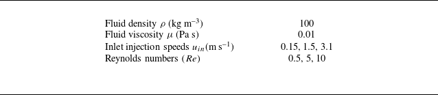
We start our comparison with figure 23, where we consider the largest investigated $Re$
value (
$Re$
value ( $Re=10.0$
) and compare the local flux
$Re=10.0$
) and compare the local flux $\boldsymbol Q$
(figure 23
d) and depth-averaged velocity
$\boldsymbol Q$
(figure 23
d) and depth-averaged velocity $\boldsymbol U=\boldsymbol Q/a$
(figure 23
a) with the equivalent quantities for the full 3-D numerical simulation, which are respectively
$\boldsymbol U=\boldsymbol Q/a$
(figure 23
a) with the equivalent quantities for the full 3-D numerical simulation, which are respectively $\boldsymbol q$
(figure 23
e) and
$\boldsymbol q$
(figure 23
e) and $\overline {\boldsymbol u}$
(figure 23
b). The probability density functions of the relative differences between the corresponding outputs of the 2-D vs 3-D models are shown in figure 23(c) for the velocities and 23(f) for the fluxes. They can be interpreted as errors made by using the depth-averaged approach. They are smaller than 10 % almost everywhere, with a peak slightly above 1 %, the mean value being 1.5 % for the error on
$\overline {\boldsymbol u}$
(figure 23
b). The probability density functions of the relative differences between the corresponding outputs of the 2-D vs 3-D models are shown in figure 23(c) for the velocities and 23(f) for the fluxes. They can be interpreted as errors made by using the depth-averaged approach. They are smaller than 10 % almost everywhere, with a peak slightly above 1 %, the mean value being 1.5 % for the error on $\boldsymbol{U}$
, and 1.2 % for the error on
$\boldsymbol{U}$
, and 1.2 % for the error on $\boldsymbol{Q}$
. In fact the errors are all the smaller as the Reynolds number is smaller, as expected due to the disappearance of inertial effects at very small Reynolds numbers. For
$\boldsymbol{Q}$
. In fact the errors are all the smaller as the Reynolds number is smaller, as expected due to the disappearance of inertial effects at very small Reynolds numbers. For $Re = 5.0$
the mean value is 1.0 % for
$Re = 5.0$
the mean value is 1.0 % for $\boldsymbol{U}$
and 0.8 % for
$\boldsymbol{U}$
and 0.8 % for $\boldsymbol{Q}$
. Lastly, for the smallest
$\boldsymbol{Q}$
. Lastly, for the smallest $Re$
case (
$Re$
case ( $Re = 0.5$
) the mean error values are 0.6 % and 0.3 % for
$Re = 0.5$
) the mean error values are 0.6 % and 0.3 % for $\boldsymbol{U}$
and
$\boldsymbol{U}$
and $\boldsymbol{Q}$
, respectively.
$\boldsymbol{Q}$
, respectively.
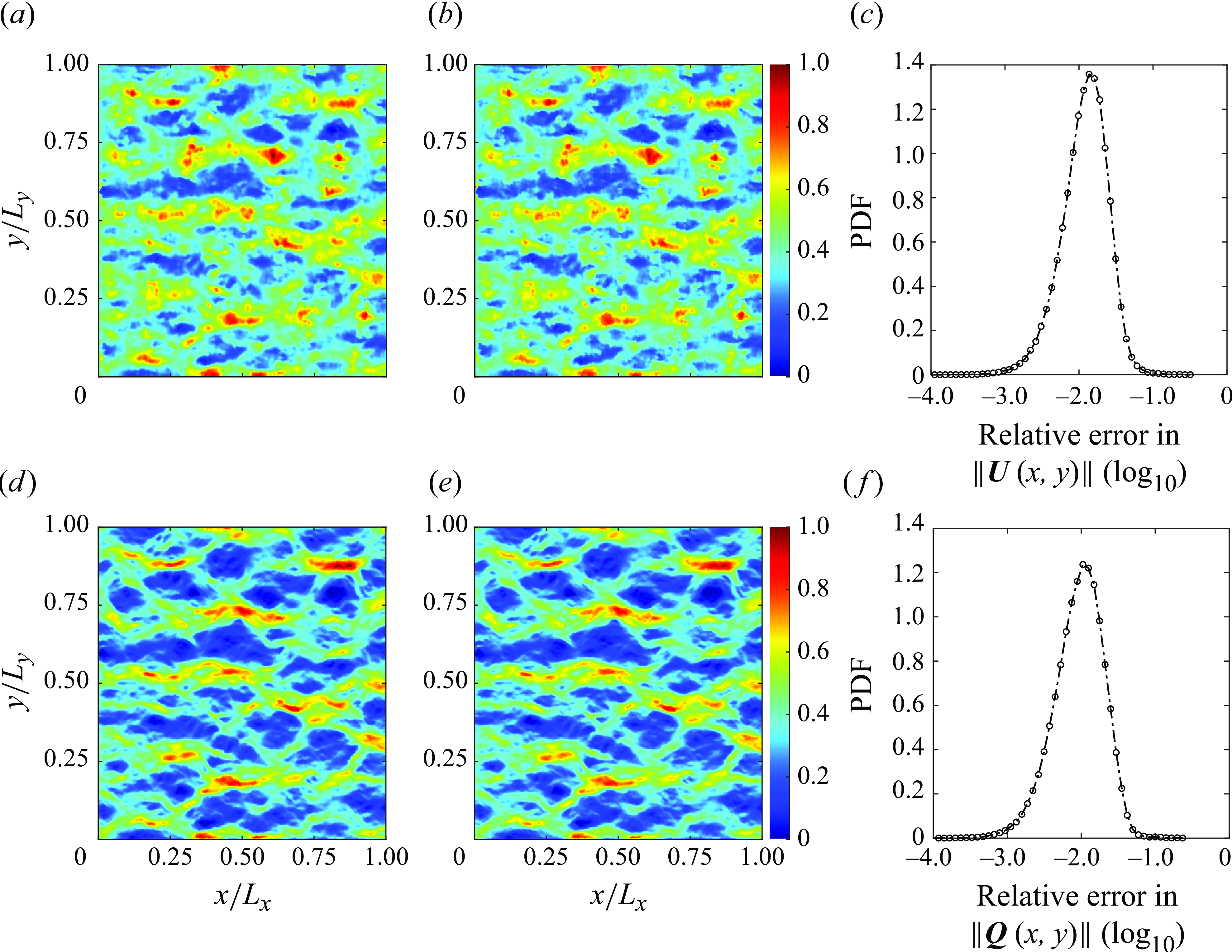
Figure 23. Spatial distribution of the velocity $\|\boldsymbol{U}(x,y)\|$
and flux
$\|\boldsymbol{U}(x,y)\|$
and flux $\|\boldsymbol{Q}(x,y)\|$
fields:
$\|\boldsymbol{Q}(x,y)\|$
fields: $(a)$
and
$(a)$
and $(d)$
from the 2-D model, and
$(d)$
from the 2-D model, and $(b)$
and
$(b)$
and $(e)$
for the depth-averaged 2-D equivalent velocity
$(e)$
for the depth-averaged 2-D equivalent velocity $\|\bar {\boldsymbol{u}}(x,y)\|$
and flux
$\|\bar {\boldsymbol{u}}(x,y)\|$
and flux $\| \boldsymbol{q}(x,y)\|$
fields from the 3-D model.
$\| \boldsymbol{q}(x,y)\|$
fields from the 3-D model. $(c, f)$
Probability density functions (PDFs) of the logarithm of the relative errors between the 2-D and 3-D models for velocity
$(c, f)$
Probability density functions (PDFs) of the logarithm of the relative errors between the 2-D and 3-D models for velocity $(c)$
and local flux
$(c)$
and local flux $(f)$
. The velocity and flux values are normalised by the corresponding maximum values from the depth-averaged 3-D fields. The dot-dashed line is simply a broken line linking the symbols. The Reynolds number is 10.
$(f)$
. The velocity and flux values are normalised by the corresponding maximum values from the depth-averaged 3-D fields. The dot-dashed line is simply a broken line linking the symbols. The Reynolds number is 10.
Next, we compare the pressure distributions across the domain for the 2-D and 3-D models. Figure 24 shows the reduced pressure field (dynamic pressure $p_{{d}}$
) distributions obtained from the 2-D (figure 24
a) and the 3-D (figure 24
b) simulations. The relative errors PDF are shown in (figure 24
c); for this particular case (
$p_{{d}}$
) distributions obtained from the 2-D (figure 24
a) and the 3-D (figure 24
b) simulations. The relative errors PDF are shown in (figure 24
c); for this particular case ( $Re=10.0$
) the peak is around 2.5 % while the mean value is 2.7 %. Overall these plots also show an excellent agreement between the 2-D depth-integrated pressure field and the reference 3-D pressure solution.
$Re=10.0$
) the peak is around 2.5 % while the mean value is 2.7 %. Overall these plots also show an excellent agreement between the 2-D depth-integrated pressure field and the reference 3-D pressure solution.
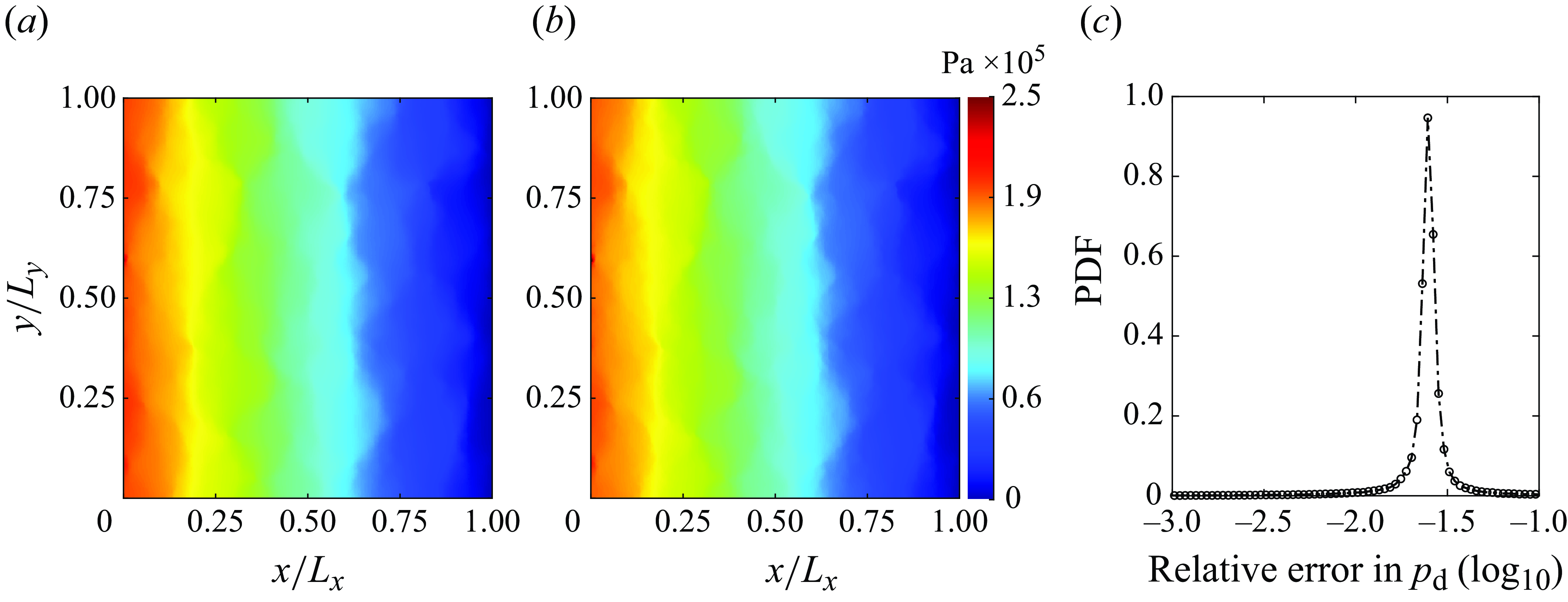
Figure 24. (a,b) Dynamic fluid pressure ( $p_{{d}}$
) distribution for the 2-D
$p_{{d}}$
) distribution for the 2-D $(a)$
and 3-D models
$(a)$
and 3-D models $(b)$
, for
$(b)$
, for $Re = 10.0$
.
$Re = 10.0$
. $(c)$
The PDFs of the logarithm of the relative errors between
$(c)$
The PDFs of the logarithm of the relative errors between $(a)$
and
$(a)$
and $(b)$
. The dot-dashed line is simply a broken line linking the symbols.
$(b)$
. The dot-dashed line is simply a broken line linking the symbols.
Lastly, we investigate to which extent our assumption of a vertical parabolic profile of velocity for the 2-D depth-integrated model is valid, in terms of properly accounting for the wall shear stresses resulting from the no-slip condition at the fracture walls (see (3.17)). The wall shear stress for the 2-D model can be obtained directly from the flux field $\boldsymbol{Q}$
through (3.17). The wall shear stress in the 3-D model, on the other hand, is computed from the 3-D velocity field
$\boldsymbol{Q}$
through (3.17). The wall shear stress in the 3-D model, on the other hand, is computed from the 3-D velocity field $\boldsymbol{u}$
through its definition (3.14). Figure 25 presents the spatial distributions of the wall shear stresses for the two models at
$\boldsymbol{u}$
through its definition (3.14). Figure 25 presents the spatial distributions of the wall shear stresses for the two models at $Re=10$
, along with the associated relative errors’ PDF. Our assumption of parabolic velocity does not hold perfectly, due both to the aperture field gradients (figure 10
c) as well as to local inertia effects which start manifesting for
$Re=10$
, along with the associated relative errors’ PDF. Our assumption of parabolic velocity does not hold perfectly, due both to the aperture field gradients (figure 10
c) as well as to local inertia effects which start manifesting for $Re\gt 1$
. Note, however, that the mean relative error in this case, is 7 %, which is not too bad. We report similar observations for the shear stress distributions other at
$Re\gt 1$
. Note, however, that the mean relative error in this case, is 7 %, which is not too bad. We report similar observations for the shear stress distributions other at $Re = 5.0$
and
$Re = 5.0$
and $Re=0.5$
, which are not shown here for the sake of brevity.
$Re=0.5$
, which are not shown here for the sake of brevity.
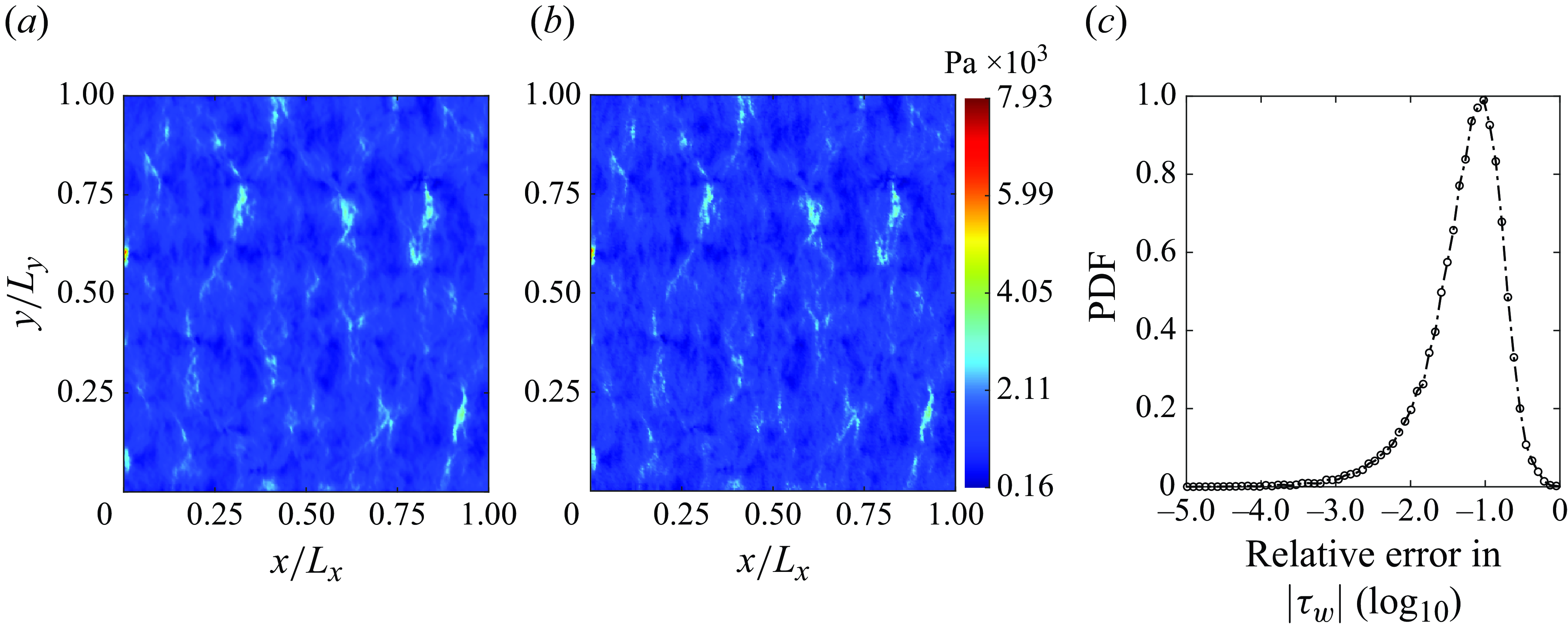
Figure 25. Wall shear stress distribution $|\boldsymbol{\tau _{{w}}}|$
, in Pa unit, resulting from the top and bottom wall surfaces of the fracture, for the 2-D
$|\boldsymbol{\tau _{{w}}}|$
, in Pa unit, resulting from the top and bottom wall surfaces of the fracture, for the 2-D $(a)$
and 3-D
$(a)$
and 3-D $(b)$
models at
$(b)$
models at $Re=10.0$
. (c) The PDFs of the logarithm of the relative errors between
$Re=10.0$
. (c) The PDFs of the logarithm of the relative errors between $(a)$
and
$(a)$
and $(b)$
are shown in
$(b)$
are shown in $(c)$
. The dot-dashed line is simply a broken line linking the symbols.
$(c)$
. The dot-dashed line is simply a broken line linking the symbols.
These observations indicate that despite some limitations, our single-phase 2-D depth-integrated model can predict single-phase flow (even weakly inertial) with good accuracy, compared with the full 3-D model results, with the advantage of a much-increased computational speed.


 Open access