


1 Introduction
Let
 $\mathcal {G}$
be a graph with edges labeled by ideals in
$\mathcal {G}$
be a graph with edges labeled by ideals in ![]() . A spline on
. A spline on
 $\mathcal {G}$
is an assignment of polynomials to vertices such that the difference of two polynomials labeling adjacent vertices must be in the corresponding ideal. The Cayley graph for a group G and generating set
$\mathcal {G}$
is an assignment of polynomials to vertices such that the difference of two polynomials labeling adjacent vertices must be in the corresponding ideal. The Cayley graph for a group G and generating set
 $S \subseteq G$
has vertex set G and edge set
$S \subseteq G$
has vertex set G and edge set
 $\{(g,gs) \mid g \in G, s \in S\}$
. When the group G is a symmetric group
$\{(g,gs) \mid g \in G, s \in S\}$
. When the group G is a symmetric group
 $S_n$
and the generating set S consists of inversions, there is a natural edge labeling for the corresponding Cayley graph. This labeled Cayley graph, and thereby the splines on it, are entirely determined by the data of the inversion graph
$S_n$
and the generating set S consists of inversions, there is a natural edge labeling for the corresponding Cayley graph. This labeled Cayley graph, and thereby the splines on it, are entirely determined by the data of the inversion graph
 $\Gamma = ([n],S)$
. This paper determines algebraic structures of splines on Cayley graphs of symmetric groups using the combinatorial data of the inversion graph
$\Gamma = ([n],S)$
. This paper determines algebraic structures of splines on Cayley graphs of symmetric groups using the combinatorial data of the inversion graph
 $\Gamma $
.
$\Gamma $
.
To discuss the results below, we begin with some notation. Let
 $\Gamma $
be a connected simple graph with vertex set
$\Gamma $
be a connected simple graph with vertex set ![]() , and identify the edges in its edge set
, and identify the edges in its edge set
 $E(\Gamma )$
with transpositions in
$E(\Gamma )$
with transpositions in
 $S_n$
. This paper studies how properties of
$S_n$
. This paper studies how properties of
 $\Gamma $
determine the algebraic structure of splines on the Cayley graph
$\Gamma $
determine the algebraic structure of splines on the Cayley graph
 $\mathcal {G}_{\Gamma }$
of
$\mathcal {G}_{\Gamma }$
of
 $S_n$
with generating set
$S_n$
with generating set
 $E(\Gamma )$
and edge label
$E(\Gamma )$
and edge label
 $(w,w(i,j)) \mapsto \left \langle t_{w(i)} - t_{w(j)} \right \rangle $
. Formally, the ring of splines is defined as
$(w,w(i,j)) \mapsto \left \langle t_{w(i)} - t_{w(j)} \right \rangle $
. Formally, the ring of splines is defined as

with (graded)
 $S_n$
-module structure
$S_n$
-module structure
 $w\cdot \bar {\rho }(v) = w\bar {\rho }(w^{-1}v)$
and (graded)
$w\cdot \bar {\rho }(v) = w\bar {\rho }(w^{-1}v)$
and (graded)
 $\mathbb {C}[t_\bullet ]$
-module structure given by multiplication.
$\mathbb {C}[t_\bullet ]$
-module structure given by multiplication.
This definition of the ring of splines generalizes the case where
 $\mathcal {G}_\Gamma $
is the moment graph of a geometric object called a regular semisimple Hessenberg variety and the ring of splines is isomorphic to the equivariant cohomology of that variety [Reference De Mari, Procesi and Shayman13, Reference Goresky, Kottwitz and MacPherson16, Reference Tymoczko28]. We call this the geometric case, and in this case, the corresponding graph
$\mathcal {G}_\Gamma $
is the moment graph of a geometric object called a regular semisimple Hessenberg variety and the ring of splines is isomorphic to the equivariant cohomology of that variety [Reference De Mari, Procesi and Shayman13, Reference Goresky, Kottwitz and MacPherson16, Reference Tymoczko28]. We call this the geometric case, and in this case, the corresponding graph
 $\Gamma $
is a Hessenberg graph, commonly characterized in algebraic combinatorics as being the indifference graph of a
$\Gamma $
is a Hessenberg graph, commonly characterized in algebraic combinatorics as being the indifference graph of a
 $3+1$
- and
$3+1$
- and
 $2+2$
-free poset. The more general setting considered in this paper allows one to spot patterns in rich algebraic structure that would otherwise be restricted for geometric reasons. For example, in the geometric case,
$2+2$
-free poset. The more general setting considered in this paper allows one to spot patterns in rich algebraic structure that would otherwise be restricted for geometric reasons. For example, in the geometric case,
 $\mathcal {M}_{\Gamma }$
is always a free module over the polynomial ring, whereas for general
$\mathcal {M}_{\Gamma }$
is always a free module over the polynomial ring, whereas for general
 $\Gamma $
, it is not.
$\Gamma $
, it is not.
The
 $S_n$
-module structure on
$S_n$
-module structure on
 $\mathcal {M}_{\Gamma }$
was first defined in the geometric case as the dot action on equivariant cohomology by Tymoczko in [Reference Tymoczko28]. There are two natural
$\mathcal {M}_{\Gamma }$
was first defined in the geometric case as the dot action on equivariant cohomology by Tymoczko in [Reference Tymoczko28]. There are two natural
 $S_n$
-equivariant quotients,
$S_n$
-equivariant quotients,
 $\mathrm {L}_{\Gamma }$
and
$\mathrm {L}_{\Gamma }$
and
 $\mathrm {R}_{\Gamma }$
, of
$\mathrm {R}_{\Gamma }$
, of
 $\mathcal {M}_{\Gamma }$
that are in fact graded
$\mathcal {M}_{\Gamma }$
that are in fact graded
 $\mathbb {C}$
-vector spaces. The graded
$\mathbb {C}$
-vector spaces. The graded
 $S_n$
-module structure of
$S_n$
-module structure of
 $\mathcal {M}_{\Gamma }$
induces graded
$\mathcal {M}_{\Gamma }$
induces graded
 $S_n$
-representations on the quotients, admitting (via the Frobenius character map
$S_n$
-representations on the quotients, admitting (via the Frobenius character map
 $\mathbf {ch}$
) two different graded symmetric functions:
$\mathbf {ch}$
) two different graded symmetric functions:
These are manifestly Schur-positive symmetric function invariants of any simple graph.
The graded symmetric functions
 $\mathbf {ch}\left (\mathrm {L}_{\Gamma }\right )$
and
$\mathbf {ch}\left (\mathrm {L}_{\Gamma }\right )$
and
 $\mathbf {ch}\left (\mathrm {R}_{\Gamma }\right )$
are historically of interest to algebraic combinatorists because of their connections to chromatic symmetric functions [Reference Brosnan and Chow8, Reference Guay-Paquet19, Reference Shareshian and Wachs25] and LLT polynomials [Reference Alexandersson and Panova3, Reference Ayzenberg and Buchstaber5, Reference Guay-Paquet19] in the geometric case. The two bases of symmetric functions we consider here are Schur functions
$\mathbf {ch}\left (\mathrm {R}_{\Gamma }\right )$
are historically of interest to algebraic combinatorists because of their connections to chromatic symmetric functions [Reference Brosnan and Chow8, Reference Guay-Paquet19, Reference Shareshian and Wachs25] and LLT polynomials [Reference Alexandersson and Panova3, Reference Ayzenberg and Buchstaber5, Reference Guay-Paquet19] in the geometric case. The two bases of symmetric functions we consider here are Schur functions
 $\{s_\lambda \}$
and homogeneous symmetric functions
$\{s_\lambda \}$
and homogeneous symmetric functions
 $\{h_\lambda \}$
. In the geometric case, two major open problems seek (1) a homogeneous basis expansion of
$\{h_\lambda \}$
. In the geometric case, two major open problems seek (1) a homogeneous basis expansion of
 $\mathbf {ch}\left (\mathrm {L}_{\Gamma }\right )$
([Reference Abreu and Nigro1, Reference Brosnan and Chow8, Reference Dahlberg12, Reference Gasharov14, Reference Guay-Paquet18, Reference Harada and Precup20, Reference Shareshian and Wachs25, Reference Stanley26], and many others), and (2) a Schur basis expansion of
$\mathbf {ch}\left (\mathrm {L}_{\Gamma }\right )$
([Reference Abreu and Nigro1, Reference Brosnan and Chow8, Reference Dahlberg12, Reference Gasharov14, Reference Guay-Paquet18, Reference Harada and Precup20, Reference Shareshian and Wachs25, Reference Stanley26], and many others), and (2) a Schur basis expansion of
 $\mathbf {ch}\left (\mathrm {R}_{\Gamma }\right )$
([Reference Alexandersson2, Reference Blasiak7, Reference Guay-Paquet19, Reference Huh, Nam and Yoo21, Reference Leclerc and Thibon22, Reference Lee23] and many others). Again, our object of study is more general, and because of this, we can identify patterns otherwise masked by geometric structure. For example, the Stanley–Stembridge conjecture [Reference Stanley and Stembridge27] claims that the homogeneous basis expansion of
$\mathbf {ch}\left (\mathrm {R}_{\Gamma }\right )$
([Reference Alexandersson2, Reference Blasiak7, Reference Guay-Paquet19, Reference Huh, Nam and Yoo21, Reference Leclerc and Thibon22, Reference Lee23] and many others). Again, our object of study is more general, and because of this, we can identify patterns otherwise masked by geometric structure. For example, the Stanley–Stembridge conjecture [Reference Stanley and Stembridge27] claims that the homogeneous basis expansion of
 $\mathbf {ch}\left (\mathrm {L}_{\Gamma }\right )$
has only nonnegative integer coefficients (h-positivity) in the geometric case. We observe below that this is not the case for general
$\mathbf {ch}\left (\mathrm {L}_{\Gamma }\right )$
has only nonnegative integer coefficients (h-positivity) in the geometric case. We observe below that this is not the case for general
 $\Gamma $
, but h-positivity seems to occur whenever
$\Gamma $
, but h-positivity seems to occur whenever
 $\mathcal {M}_{\Gamma }$
is a free module over
$\mathcal {M}_{\Gamma }$
is a free module over
 $\mathbb {C}[t_\bullet ]$
.
$\mathbb {C}[t_\bullet ]$
.
This paper begins with several fundamental properties of
 $\mathcal {M}_{\Gamma }$
. First, we establish the algebraic structure of
$\mathcal {M}_{\Gamma }$
. First, we establish the algebraic structure of
 $\mathcal {M}_{\Gamma }$
as an invariant of the graph
$\mathcal {M}_{\Gamma }$
as an invariant of the graph
 $\Gamma $
.
$\Gamma $
.
Lemma 1.1. An isomorphism of graphs
 $\Gamma \cong \Gamma '$
induces a ring isomorphism of splines
$\Gamma \cong \Gamma '$
induces a ring isomorphism of splines
 $\mathcal {M}_{\Gamma } \cong \mathcal {M}_{\Gamma '}$
and equality of graded symmetric functions:
$\mathcal {M}_{\Gamma } \cong \mathcal {M}_{\Gamma '}$
and equality of graded symmetric functions:
 $\mathbf {ch}\left (\mathrm {L}_{\Gamma }\right ) = \mathbf {ch}\left (\mathrm {L}_{\Gamma '}\right )$
and
$\mathbf {ch}\left (\mathrm {L}_{\Gamma }\right ) = \mathbf {ch}\left (\mathrm {L}_{\Gamma '}\right )$
and
 $\mathbf {ch}\left (\mathrm {R}_{\Gamma }\right ) = \mathbf {ch}\left (\mathrm {R}_{\Gamma '}\right )$
.
$\mathbf {ch}\left (\mathrm {R}_{\Gamma }\right ) = \mathbf {ch}\left (\mathrm {R}_{\Gamma '}\right )$
.
In particular, Lemma 1.1 shows that the graded symmetric functions
 $\mathbf {ch}\left (\mathrm {L}_{\Gamma }\right )$
and
$\mathbf {ch}\left (\mathrm {L}_{\Gamma }\right )$
and
 $\mathbf {ch}\left (\mathrm {R}_{\Gamma }\right )$
are (Schur-positive) invariants of unlabeled simple graphs. Lemma 1.1 is proved via Propositions 2.18 and 2.20 below.
$\mathbf {ch}\left (\mathrm {R}_{\Gamma }\right )$
are (Schur-positive) invariants of unlabeled simple graphs. Lemma 1.1 is proved via Propositions 2.18 and 2.20 below.
Then when
 $\Gamma $
is a tree, we determine explicit ring and module generators of
$\Gamma $
is a tree, we determine explicit ring and module generators of
 $\mathcal {M}_{\Gamma }$
called coset splines (Definition 3.4).
$\mathcal {M}_{\Gamma }$
called coset splines (Definition 3.4).
Theorem 1.2. If
 $\Gamma $
is a tree, then the set of coset splines is a
$\Gamma $
is a tree, then the set of coset splines is a
 $\mathbb {C}[t_\bullet ]$
-module generating set of
$\mathbb {C}[t_\bullet ]$
-module generating set of
 $\mathcal {M}_{\Gamma }$
, and the set of linear and constant coset splines is a ring generating set of
$\mathcal {M}_{\Gamma }$
, and the set of linear and constant coset splines is a ring generating set of
 $\mathcal {M}_{\Gamma }$
.
$\mathcal {M}_{\Gamma }$
.
Since they generate, one can compute
 $\mathcal {M}_{\Gamma }$
explicitly with coset splines using a computer algebra system. Theorem 1.2 is Theorem 3.7 and Corollary 3.8 below.
$\mathcal {M}_{\Gamma }$
explicitly with coset splines using a computer algebra system. Theorem 1.2 is Theorem 3.7 and Corollary 3.8 below.
We use Theorem 1.2 to show that
 $\mathcal {M}_{\Gamma }$
is not always a free
$\mathcal {M}_{\Gamma }$
is not always a free
 $\mathbb {C}[t_\bullet ]$
-module, and
$\mathbb {C}[t_\bullet ]$
-module, and
 $\mathbf {ch}\left (\mathrm {L}_{\Gamma }\right )$
is not always h-positive (see Appendix A). One example is if
$\mathbf {ch}\left (\mathrm {L}_{\Gamma }\right )$
is not always h-positive (see Appendix A). One example is if
 $\Gamma = \left ([4],\{(1,4),(2,4),(3,4)\}\right )$
, then
$\Gamma = \left ([4],\{(1,4),(2,4),(3,4)\}\right )$
, then
 $\mathcal {M}_{\Gamma }$
is not a free module and
$\mathcal {M}_{\Gamma }$
is not a free module and
 $\mathbf {ch}\left (\mathrm {L}_{\Gamma }\right )_2$
is not h-positive. This also confirms that
$\mathbf {ch}\left (\mathrm {L}_{\Gamma }\right )_2$
is not h-positive. This also confirms that
 $\mathcal {M}_{\Gamma }$
is not always the equivariant cohomology of an (equivariantly formal) algebraic variety as in [Reference Goresky, Kottwitz and MacPherson16], since in that case,
$\mathcal {M}_{\Gamma }$
is not always the equivariant cohomology of an (equivariantly formal) algebraic variety as in [Reference Goresky, Kottwitz and MacPherson16], since in that case,
 $\mathcal {M}_{\Gamma }$
is a free
$\mathcal {M}_{\Gamma }$
is a free
 $\mathbb {C}[t_\bullet ]$
-module.
$\mathbb {C}[t_\bullet ]$
-module.
Our next main results, Theorems 1.3 and 1.4 below, explicitly compute certain graded pieces of the symmetric functions
 $\mathbf {ch}\left (\mathrm {L}_{\Gamma }\right )$
and
$\mathbf {ch}\left (\mathrm {L}_{\Gamma }\right )$
and
 $\mathbf {ch}\left (\mathrm {R}_{\Gamma }\right )$
. Specifically, we determine when graded pieces of
$\mathbf {ch}\left (\mathrm {R}_{\Gamma }\right )$
. Specifically, we determine when graded pieces of
 $\mathbf {ch}\left (\mathrm {L}_{\Gamma }\right )$
and
$\mathbf {ch}\left (\mathrm {L}_{\Gamma }\right )$
and
 $\mathbf {ch}\left (\mathrm {R}_{\Gamma }\right )$
are equal to
$\mathbf {ch}\left (\mathrm {R}_{\Gamma }\right )$
are equal to
 $\mathbf {ch}\left (\mathrm {L}_{K_n}\right )$
and
$\mathbf {ch}\left (\mathrm {L}_{K_n}\right )$
and
 $\mathbf {ch}\left (\mathrm {R}_{K_n}\right )$
where
$\mathbf {ch}\left (\mathrm {R}_{K_n}\right )$
where
 $K_n$
is the complete graph (
$K_n$
is the complete graph (
 $\Gamma = K_n$
is a very special geometric case), and we compute
$\Gamma = K_n$
is a very special geometric case), and we compute
 $\mathbf {ch}\left (\mathrm {L}_{\Gamma }\right )_1$
and
$\mathbf {ch}\left (\mathrm {L}_{\Gamma }\right )_1$
and
 $\mathbf {ch}\left (\mathrm {R}_{\Gamma }\right )_1$
for all connected graphs
$\mathbf {ch}\left (\mathrm {R}_{\Gamma }\right )_1$
for all connected graphs
 $\Gamma $
.
$\Gamma $
.
For a variety of reasons, for example by formulae in [Reference Shareshian and Wachs25] or by some geometric observations, in the geometric case, it is straightforward to tell from a Hessenberg graph H whether the symmetric function
 $\mathbf {ch}\left (\mathrm {L}_{H}\right )_d$
corresponds to a trivial representation. We achieve an analogous result for arbitrary graphs. The k-connectivity (Definition 2.2) of a graph is a combinatorial invariant that measures how many vertices can be removed from a graph before it might become disconnected.
$\mathbf {ch}\left (\mathrm {L}_{H}\right )_d$
corresponds to a trivial representation. We achieve an analogous result for arbitrary graphs. The k-connectivity (Definition 2.2) of a graph is a combinatorial invariant that measures how many vertices can be removed from a graph before it might become disconnected.
Theorem 1.3. Let
 $\Gamma $
be a connected simple graph. The following are equivalent:
$\Gamma $
be a connected simple graph. The following are equivalent:
-
1) The graph
 $\Gamma $
is k-connected.
$\Gamma $
is k-connected. -
2) For all
$d<k$
, the symmetric function
$\mathbf {ch}\left (\mathrm {L}_{\Gamma }\right )_d$
corresponds to a trivial representation. -
3) For all
$d<k$
, the d-th graded piece of
$\mathcal {M}_{\Gamma }$
is isomorphic to the d-th graded piece of
$\mathcal {M}_{K_n}$
, where
$K_n$
is the complete graph on n vertices.


Geometrically, the d-th graded piece of
 $\mathcal {M}_{K_n}$
is isomorphic to the
$\mathcal {M}_{K_n}$
is isomorphic to the
 $2d$
-th equivariant cohomology of the full flag variety and is thus spanned by equivariant Schubert classes whose spline formula is given in [Reference Billey6]. Theorem 1.3 is a consequence of Theorem 4.2 below.
$2d$
-th equivariant cohomology of the full flag variety and is thus spanned by equivariant Schubert classes whose spline formula is given in [Reference Billey6]. Theorem 1.3 is a consequence of Theorem 4.2 below.
When
 $\Gamma $
is a Hessenberg graph, the first graded piece of
$\Gamma $
is a Hessenberg graph, the first graded piece of
 $\mathbf {ch}\left (\mathrm {L}_{\Gamma }\right )$
has been computed in a variety of ways. The Schur expansion is computed by counting P-tableaux [Reference Shareshian and Wachs25]. Expansions in the homogeneous basis have been computed with P-tableaux [Reference Chow11], geometrically [Reference Cho, Hong and Lee10], as well as with splines [Reference Ayzenberg, Masuda and Sato4]. Our methods here most directly generalize those in [Reference Ayzenberg, Masuda and Sato4].
$\mathbf {ch}\left (\mathrm {L}_{\Gamma }\right )$
has been computed in a variety of ways. The Schur expansion is computed by counting P-tableaux [Reference Shareshian and Wachs25]. Expansions in the homogeneous basis have been computed with P-tableaux [Reference Chow11], geometrically [Reference Cho, Hong and Lee10], as well as with splines [Reference Ayzenberg, Masuda and Sato4]. Our methods here most directly generalize those in [Reference Ayzenberg, Masuda and Sato4].
Theorem 1.4. D Let
 $\Gamma $
be any connected simple graph. The first-degree pieces of the graded symmetric functions
$\Gamma $
be any connected simple graph. The first-degree pieces of the graded symmetric functions
 $\mathbf {ch}\left (\mathrm {L}_{\Gamma }\right )$
and
$\mathbf {ch}\left (\mathrm {L}_{\Gamma }\right )$
and
 $\mathbf {ch}\left (\mathrm {R}_{\Gamma }\right )$
can be computed in both the Schur and homogeneous bases of symmetric functions from the data of (1) cut edges of
$\mathbf {ch}\left (\mathrm {R}_{\Gamma }\right )$
can be computed in both the Schur and homogeneous bases of symmetric functions from the data of (1) cut edges of
 $\Gamma $
and (2) cut vertices of
$\Gamma $
and (2) cut vertices of
 $\Gamma $
and the number of connected components those vertices separate.
$\Gamma $
and the number of connected components those vertices separate.
Formally, there exist a subset
 $E_1$
of cut edges, a subset
$E_1$
of cut edges, a subset
 $E_2$
of 2-connected subgraphs, a nonnegative integer
$E_2$
of 2-connected subgraphs, a nonnegative integer
 $k \in \mathbb { N}$
, and a function
$k \in \mathbb { N}$
, and a function
 $e \mapsto \lambda _e$
from
$e \mapsto \lambda _e$
from
 $E_1$
to the set of partitions of n, such that
$E_1$
to the set of partitions of n, such that
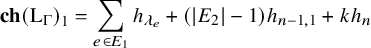 $$\begin{align*}\mathbf{ch}\left(\mathrm{L}_{\Gamma}\right)_1 = \sum_{e \in E_1} h_{\lambda_e} + \left(\left| E_2 \right|-1\right) h_{n-1,1} + kh_n \end{align*}$$
and
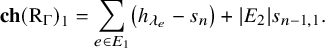 $$\begin{align*}\mathbf{ch}\left(\mathrm{R}_{\Gamma}\right)_1 = \sum_{e \in E_1}\left(h_{\lambda_e} - s_n\right) +\left| E_2 \right| s_{n-1,1}. \end{align*}$$
Theorem 1.4 is Theorem 9.2 and Corollary 9.3 below. The subsets
 $E_1$
and
$E_1$
and
 $E_2$
are defined using a combinatorial construction from the block-cut tree (Definition 6.2) of
$E_2$
are defined using a combinatorial construction from the block-cut tree (Definition 6.2) of
 $\Gamma $
in Section 8.
$\Gamma $
in Section 8.
The paper is structured as follows. Section 2 constructs
 $\mathcal {M}_{\Gamma }$
and proves some of the fundamental algebraic properties, including the isomorphism of Lemma 1.1. Section 3 builds tools for computing spline conditions from paths in
$\mathcal {M}_{\Gamma }$
and proves some of the fundamental algebraic properties, including the isomorphism of Lemma 1.1. Section 3 builds tools for computing spline conditions from paths in
 $\Gamma $
and
$\Gamma $
and
 $\mathcal {G}_\Gamma $
. It also contains the construction of coset splines for trees and the proof that coset splines generate
$\mathcal {G}_\Gamma $
. It also contains the construction of coset splines for trees and the proof that coset splines generate
 $\mathcal {M}_{\Gamma }$
, Theorem 1.2 above. Section 4 leverages the tools in Section 3 to prove our result on k-connectedness, Theorem 1.3 above. Sections 5, 6, 7, 8 and 9 are all to compute the representations in Theorem 1.4 above. Section 5 defines a set of linear splines on the graph
$\mathcal {M}_{\Gamma }$
, Theorem 1.2 above. Section 4 leverages the tools in Section 3 to prove our result on k-connectedness, Theorem 1.3 above. Sections 5, 6, 7, 8 and 9 are all to compute the representations in Theorem 1.4 above. Section 5 defines a set of linear splines on the graph
 $\mathcal {G}_\Gamma $
and proves some linear relations within that set. Section 6 reduces the computation to a subclass of graphs
$\mathcal {G}_\Gamma $
and proves some linear relations within that set. Section 6 reduces the computation to a subclass of graphs
 $\Gamma $
that will be used in all of the remaining sections. Section 7 proves that the set of splines from Section 5 is in fact a
$\Gamma $
that will be used in all of the remaining sections. Section 7 proves that the set of splines from Section 5 is in fact a
 $\mathbb {C}$
-spanning set for linear splines, and Section 8 computes the
$\mathbb {C}$
-spanning set for linear splines, and Section 8 computes the
 $\mathbb {C}$
-dimension of this space. Finally, Section 9 computes the first graded piece of
$\mathbb {C}$
-dimension of this space. Finally, Section 9 computes the first graded piece of
 $\mathbf {ch}\left (\mathrm {L}_{\Gamma }\right )$
and
$\mathbf {ch}\left (\mathrm {L}_{\Gamma }\right )$
and
 $\mathbf {ch}\left (\mathrm {R}_{\Gamma }\right )$
, Theorem 1.4. Appendix A contains a table of
$\mathbf {ch}\left (\mathrm {R}_{\Gamma }\right )$
, Theorem 1.4. Appendix A contains a table of
 $\mathbf {ch}\left (\mathrm {L}_{\Gamma }\right )$
and
$\mathbf {ch}\left (\mathrm {L}_{\Gamma }\right )$
and
 $\mathbf {ch}\left (\mathrm {R}_{\Gamma }\right )$
for graphs with
$\mathbf {ch}\left (\mathrm {R}_{\Gamma }\right )$
for graphs with
 $3$
or
$3$
or
 $4$
vertices and a table of the rank-generating functions for graphs of size
$4$
vertices and a table of the rank-generating functions for graphs of size
 $5$
(which gives the graded dimension of the representations).
$5$
(which gives the graded dimension of the representations).
2 Background
There is a natural action of the symmetric group
 $S_n$
on the polynomial ring
$S_n$
on the polynomial ring
 $\mathbb {C}[t_\bullet ]$
by
$\mathbb {C}[t_\bullet ]$
by
 $$ \begin{align} w f\left(t_1,\ldots,t_n\right) \mapsto f\left(t_{w(1)},\ldots,t_{w(n)}\right). \end{align} $$
We use both one-line and cycle notation for elements of
 $S_n$
. We denote a permutation’s cycle notation with parentheses and commas, and its one-line notation without, so that
$S_n$
. We denote a permutation’s cycle notation with parentheses and commas, and its one-line notation without, so that
 $(1,2,3)=231$
.
$(1,2,3)=231$
.
2.1 Graphs: simple and Cayley
This subsection establishes the basic definitions, results and notation from graph theory needed below. A graph is a tuple
 $\Gamma = (V,E)$
where V is the set of vertices and
$\Gamma = (V,E)$
where V is the set of vertices and
 $E \subset V\times V$
is the set of edges. Graphs here are understood to be undirected and simple (i.e., finite, loopless and without multiple edges). We will always take
$E \subset V\times V$
is the set of edges. Graphs here are understood to be undirected and simple (i.e., finite, loopless and without multiple edges). We will always take
 $\Gamma $
to be connected and may remind the reader of this assumption where particularly important. Write
$\Gamma $
to be connected and may remind the reader of this assumption where particularly important. Write
 $E(\Gamma )$
for the edge set of a graph
$E(\Gamma )$
for the edge set of a graph
 $\Gamma $
and
$\Gamma $
and
 $V(\Gamma )$
for the vertex set. Inclusion
$V(\Gamma )$
for the vertex set. Inclusion
 $v \in \Gamma $
means
$v \in \Gamma $
means
 $v \in V(\Gamma )$
.
$v \in V(\Gamma )$
.
If the vertex set V has some natural linear order (in particular, when
 $V = [n]$
), then an edge between vertices
$V = [n]$
), then an edge between vertices
 $i < j$
will always be written with the lower vertex first
$i < j$
will always be written with the lower vertex first
 $(i,j)$
, unless explicitly stated otherwise. Note that these edges are undirected, so an edge
$(i,j)$
, unless explicitly stated otherwise. Note that these edges are undirected, so an edge
 $(i,j)$
is the same as an edge
$(i,j)$
is the same as an edge
 $(j,i)$
.
$(j,i)$
.
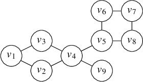
We denote graphs pictorially with circles as vertices and lines as edges between them; for example, we would display a particular graph
 $\Gamma $
on
$\Gamma $
on
 $9$
vertices as
$9$
vertices as
The induced subgraph of
 $\Gamma $
with vertex set
$\Gamma $
with vertex set
 $V \setminus A$
is
$V \setminus A$
is ![]() , where
, where
 $E' = E \cap \left ( V \setminus A \times V \setminus A\right )$
. We write
$E' = E \cap \left ( V \setminus A \times V \setminus A\right )$
. We write
 $\Gamma - v$
for
$\Gamma - v$
for
 $\Gamma \setminus \{v\}$
. When collapsing a subgraph in drawing, we reference the subgraph in a square to distinguish that there are multiple vertices being referenced, and double lines connecting to acknowledge the possibility of multiple edges. For example, we may display
$\Gamma \setminus \{v\}$
. When collapsing a subgraph in drawing, we reference the subgraph in a square to distinguish that there are multiple vertices being referenced, and double lines connecting to acknowledge the possibility of multiple edges. For example, we may display
 $\Gamma $
above as
$\Gamma $
above as
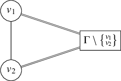
if the structure within
 $\Gamma \setminus \left \{v_1 ,v_2\right \}$
is not needed.
$\Gamma \setminus \left \{v_1 ,v_2\right \}$
is not needed.
Definition 2.1. For a graph
 $\Gamma $
, a set
$\Gamma $
, a set
 $A \subset V(\Gamma )$
is a cut set if
$A \subset V(\Gamma )$
is a cut set if
 $\Gamma \setminus A$
is disconnected. Similarly,
$\Gamma \setminus A$
is disconnected. Similarly,
 $v \in V(\Gamma )$
is a cut vertex of
$v \in V(\Gamma )$
is a cut vertex of
 $\Gamma $
(denoted
$\Gamma $
(denoted
 $v \vdash \Gamma $
) if
$v \vdash \Gamma $
) if
 $\Gamma - v$
is disconnected.
$\Gamma - v$
is disconnected.
An edge
 $e \in E(\Gamma )$
is a cut edge if the graph
$e \in E(\Gamma )$
is a cut edge if the graph
 $(V(\Gamma ),E(\Gamma )\setminus \{e\})$
is disconnected.
$(V(\Gamma ),E(\Gamma )\setminus \{e\})$
is disconnected.
A path in
 $\Gamma $
from vertex
$\Gamma $
from vertex
 $v_0$
to vertex
$v_0$
to vertex
 $v_\ell $
of length
$v_\ell $
of length
 $\ell $
is a sequence of vertices
$\ell $
is a sequence of vertices
 $(v_0,v_1,...,v_\ell )$
, where
$(v_0,v_1,...,v_\ell )$
, where
 $(v_k,v_{k+1}) \in E(\Gamma )$
for
$(v_k,v_{k+1}) \in E(\Gamma )$
for
 $k=0,...,\ell -1$
. Define the distance
$k=0,...,\ell -1$
. Define the distance
 $d(v,w)$
between v and w as the minimum length over all paths from v to w, and let
$d(v,w)$
between v and w as the minimum length over all paths from v to w, and let ![]() if no such path exists.
if no such path exists.
Definition 2.2. A graph
 $\Gamma = (V,E)$
is k-connected if
$\Gamma = (V,E)$
is k-connected if
 $\Gamma \setminus A$
is connected for all
$\Gamma \setminus A$
is connected for all
 $A \subset V$
such that
$A \subset V$
such that
 $\left | A \right | \leq k-1$
.
$\left | A \right | \leq k-1$
.
In other words, a graph is k-connected if there exists no cut set A where
 $\left | A \right | <k$
. The following is an equivalent characterization used in
$\left | A \right | <k$
. The following is an equivalent characterization used in
 $\S $
4.
$\S $
4.
Theorem 2.3 (Menger’s Theorem).
A graph
 $\Gamma $
is k-connected if and only if for every pair of vertices
$\Gamma $
is k-connected if and only if for every pair of vertices
 $i,j \in \Gamma $
, there exist at least k vertex-disjoint paths from i to j.
$i,j \in \Gamma $
, there exist at least k vertex-disjoint paths from i to j.
An R-labeled graph is a tuple
 $(V,E,L)$
, where
$(V,E,L)$
, where
 $(V,E)$
is a graph and L is a function
$(V,E)$
is a graph and L is a function
 $L \colon E \to R$
for some set R. A Cayley graph of a group G and a set of generators S is the graph
$L \colon E \to R$
for some set R. A Cayley graph of a group G and a set of generators S is the graph
 $\left (G,\{(g,h) \mid g^{-1}h \in S\}\right )$
. Cayley graphs are usually directed graphs, but all generators considered here will be involutions, and so the Cayley graphs will be undirected simple graphs. Note that
$\left (G,\{(g,h) \mid g^{-1}h \in S\}\right )$
. Cayley graphs are usually directed graphs, but all generators considered here will be involutions, and so the Cayley graphs will be undirected simple graphs. Note that
 $g^{-1}h \in S$
if and only if
$g^{-1}h \in S$
if and only if
 $h=gs$
for
$h=gs$
for
 $s \in S$
, so edges in a Cayley graph correspond to right multiplication by generators.
$s \in S$
, so edges in a Cayley graph correspond to right multiplication by generators.
This paper concerns graphs
 $\Gamma $
on vertex set
$\Gamma $
on vertex set
 $[n]$
and labeled Cayley graphs of the symmetric group with generators being some set of transpositions. The edge labels are principle ideals in
$[n]$
and labeled Cayley graphs of the symmetric group with generators being some set of transpositions. The edge labels are principle ideals in
 $\mathbb {C}[t_\bullet ]$
.
$\mathbb {C}[t_\bullet ]$
.
Definition 2.4. Let
 $\Gamma $
be a graph on
$\Gamma $
be a graph on
 $[n]$
. Identify each edge
$[n]$
. Identify each edge
 $(i,j) \in E(\Gamma )$
with the transposition
$(i,j) \in E(\Gamma )$
with the transposition
 $(i,j) \in S_n$
. The labeled Cayley graph associated to
$(i,j) \in S_n$
. The labeled Cayley graph associated to
 $\Gamma $
is
$\Gamma $
is
 $\mathcal {G}_\Gamma := (\mathcal {V},\mathcal {E},\mathcal {L})$
, where
$\mathcal {G}_\Gamma := (\mathcal {V},\mathcal {E},\mathcal {L})$
, where
-
•
$\mathcal {V} = S_n$
, -
•
$\mathcal {E} = \{(w,v) \mid w^{-1}v \in E(\Gamma )\}$
, and -
•
$\mathcal {L}(w,v) = \left \langle t_i-t_j \right \rangle $
, where
$(i,j) = wv^{-1}$
.


Note
 $w^{-1}v$
is conjugate to
$w^{-1}v$
is conjugate to
 $wv^{-1}$
, so if
$wv^{-1}$
, so if
 $w = v(i,j)$
, then
$w = v(i,j)$
, then
 $\mathcal {L}(w,v) = \langle t_{w(i)}-t_{w(j)}\rangle = \langle t_{v(i)}-t_{v(j)}\rangle .$
Note also that
$\mathcal {L}(w,v) = \langle t_{w(i)}-t_{w(j)}\rangle = \langle t_{v(i)}-t_{v(j)}\rangle .$
Note also that
 $\mathcal {L}$
is defined whenever
$\mathcal {L}$
is defined whenever
 $wv^{-1}$
is a transposition.
$wv^{-1}$
is a transposition.
Example 2.5. Let
 $\Gamma = \left ([3],\{(1,2),(2,3)\}\right )$
. Then
$\Gamma = \left ([3],\{(1,2),(2,3)\}\right )$
. Then
 $\mathcal {G}_\Gamma $
has vertex set
$\mathcal {G}_\Gamma $
has vertex set
 $S_3$
, edges
$S_3$
, edges
 $\{(w,v) \mid w^{-1}v \in \{(1,2),(2,3)\}$
, and labels of the form
$\{(w,v) \mid w^{-1}v \in \{(1,2),(2,3)\}$
, and labels of the form
 $\langle t_i-t_j\rangle $
, where
$\langle t_i-t_j\rangle $
, where
 $i,j \in [3]$
. Below is
$i,j \in [3]$
. Below is
 $\mathcal {G}_\Gamma $
, with labeling ideals denoted by generators.
$\mathcal {G}_\Gamma $
, with labeling ideals denoted by generators.
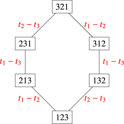
Consider the edge
 $(132,312)$
. These permutations have their first and second positions swapped, corresponding to right multiplication by
$(132,312)$
. These permutations have their first and second positions swapped, corresponding to right multiplication by
 $(1,2) \in E(\Gamma )$
. The edge is labeled
$(1,2) \in E(\Gamma )$
. The edge is labeled
 $\langle t_1-t_3\rangle $
because these permutations have the entries
$\langle t_1-t_3\rangle $
because these permutations have the entries
 $1$
and
$1$
and
 $3$
swapped, corresponding to left multiplication by
$3$
swapped, corresponding to left multiplication by
 $(1,3)$
.
$(1,3)$
.
The
 $\Gamma $
-length of a permutation
$\Gamma $
-length of a permutation
 $w \in S_n$
is
$w \in S_n$
is
This is also the value of
 $d(e,w)$
in
$d(e,w)$
in
 $\mathcal {G}_\Gamma $
. When
$\mathcal {G}_\Gamma $
. When
 $\Gamma $
is the path graph,
$\Gamma $
is the path graph,
 $\Gamma $
-length is the traditional length function on permutations.
$\Gamma $
-length is the traditional length function on permutations.
2.2 Splines
This section introduces the ring of splines on a labeled Cayley graph. The lemmas in this subsection are well known and straightforward, but we include proofs for completeness.
Definition 2.6. Let
 $\Gamma $
be a graph on
$\Gamma $
be a graph on
 $[n]$
. A spline on
$[n]$
. A spline on
 $\mathcal {G}_\Gamma $
is a function
$\mathcal {G}_\Gamma $
is a function
 $\bar {\rho } \colon S_n \to \mathbb {C}[t_\bullet ]$
such that
$\bar {\rho } \colon S_n \to \mathbb {C}[t_\bullet ]$
such that
 $\bar {\rho }(w) - \bar {\rho }(v) \in \mathcal {L}(w,v)$
whenever
$\bar {\rho }(w) - \bar {\rho }(v) \in \mathcal {L}(w,v)$
whenever
 $(w,v) \in E\left (\mathcal {G}_\Gamma \right )$
. The support of the spline
$(w,v) \in E\left (\mathcal {G}_\Gamma \right )$
. The support of the spline
 $\bar {\rho }$
is the set
$\bar {\rho }$
is the set ![]() .
.
To distinguish from polynomials, we always denote a spline with a bar.
Example 2.7. Again, consider
 $\Gamma = \left ([3],\{(1,2),(2,3)\}\right )$
. Drawn below (omitting edge-labels) are three examples of splines on
$\Gamma = \left ([3],\{(1,2),(2,3)\}\right )$
. Drawn below (omitting edge-labels) are three examples of splines on
 $\mathcal {G}_\Gamma $
.
$\mathcal {G}_\Gamma $
.
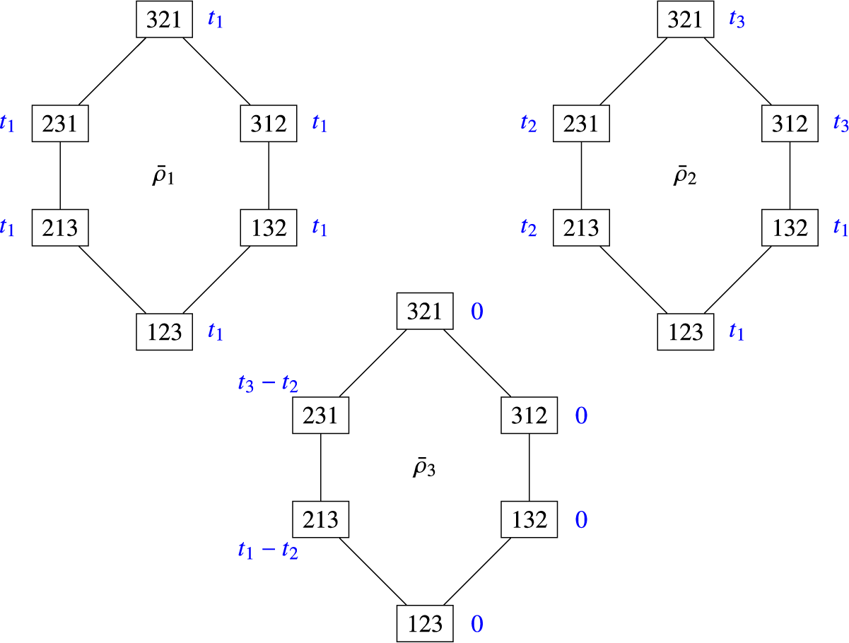
So
 $\bar {\rho }_1(w) = t_1$
for all
$\bar {\rho }_1(w) = t_1$
for all
 $w \in S_3$
,
$w \in S_3$
,
 $\bar {\rho }_2(w) = t_{w(1)}$
for all
$\bar {\rho }_2(w) = t_{w(1)}$
for all
 $w \in S_3$
, and
$w \in S_3$
, and
 ${ \bar {\rho _3}(w) = \begin {cases} t_1-t_2 & \text {if }w = 213 \\ t_3-t_2 & \text {if }w = 231 \\ 0 & \text {otherwise.} \end {cases}}$
The set of splines is closed under addition, as well as multiplication.
Lemma 2.8. Let
 $\Gamma $
be a graph on
$\Gamma $
be a graph on
 $[n]$
. If
$[n]$
. If
 $\bar {\rho }$
and
$\bar {\rho }$
and
 $\bar {\sigma }$
are splines on
$\bar {\sigma }$
are splines on
 $\mathcal {G}_\Gamma $
, then so is
$\mathcal {G}_\Gamma $
, then so is
 $\bar {\sigma }\bar {\rho }$
, the spline constructed via pointwise multiplication.
$\bar {\sigma }\bar {\rho }$
, the spline constructed via pointwise multiplication.
Proof. Let
 $(w,v) \in E(\mathcal {G}_\Gamma )$
. By assumption,
$(w,v) \in E(\mathcal {G}_\Gamma )$
. By assumption,
 $\bar {\rho }(w)-\bar {\rho }(v) \in \mathcal {L}(w,v)$
and
$\bar {\rho }(w)-\bar {\rho }(v) \in \mathcal {L}(w,v)$
and
 $\bar {\sigma }(w)-\bar {\sigma }(v) \in \mathcal {L}(w,v)$
. We have
$\bar {\sigma }(w)-\bar {\sigma }(v) \in \mathcal {L}(w,v)$
. We have
 $$ \begin{align*} \bar{\rho}(w)\bar{\sigma}(w) - \bar{\rho}(v)\bar{\sigma}(v) &= \bar{\rho}(w)\bar{\sigma}(w) - \bar{\sigma}(v)\bar{\rho}(w) +\bar{\sigma}(v)\bar{\rho}(w) - \bar{\rho}(v)\bar{\sigma}(v) \\ &= \bar{\rho}(w)\left(\bar{\sigma}(w) - \bar{\sigma}(v)\right) +\bar{\sigma}(v)\left(\bar{\rho}(w) - \bar{\rho}(v)\right), \end{align*} $$
and the sum is clearly in
 $\mathcal {L}(w,v)$
.
$\mathcal {L}(w,v)$
.
Definition 2.9. The ring of splines on
 $\mathcal {G}_\Gamma $
is the subring
$\mathcal {G}_\Gamma $
is the subring
of
 ${ \prod _{w \in S_n} \mathbb {C}[t_\bullet ]}$
with pointwise addition and multiplication.
${ \prod _{w \in S_n} \mathbb {C}[t_\bullet ]}$
with pointwise addition and multiplication.
Lemma 2.10. The ring
 $\mathcal {M}_{\Gamma }$
is graded by degree, so
$\mathcal {M}_{\Gamma }$
is graded by degree, so
 ${ \mathcal {M}_{\Gamma } = \bigoplus _{i \geq 0} \mathcal {M}_{\Gamma }^i}$
.
${ \mathcal {M}_{\Gamma } = \bigoplus _{i \geq 0} \mathcal {M}_{\Gamma }^i}$
.
Proof. Let
 $\bar {\rho }$
be a spline in
$\bar {\rho }$
be a spline in
 $\mathcal {M}_{\Gamma }$
and let
$\mathcal {M}_{\Gamma }$
and let
 $\bar {\rho }_k(w)$
be the k-th graded piece of the polynomial
$\bar {\rho }_k(w)$
be the k-th graded piece of the polynomial
 $\bar {\rho }(w)$
. We aim to show that
$\bar {\rho }(w)$
. We aim to show that
 $\bar {\rho }_k$
is a spline as well. For each
$\bar {\rho }_k$
is a spline as well. For each
 $(w,v) \in E(\mathcal {G}_\Gamma )$
, the ideal
$(w,v) \in E(\mathcal {G}_\Gamma )$
, the ideal
 $\mathcal {L}(w,v)$
is a homogeneous ideal. Thus,
$\mathcal {L}(w,v)$
is a homogeneous ideal. Thus,
 $\bar {\rho }(w)-\bar {\rho }(v) \in \mathcal {L}(w,v)$
, and it follows that
$\bar {\rho }(w)-\bar {\rho }(v) \in \mathcal {L}(w,v)$
, and it follows that
 $\bar {\rho }_k(w)-\bar {\rho }_k(v) \in \mathcal {L}(w,v)$
, so
$\bar {\rho }_k(w)-\bar {\rho }_k(v) \in \mathcal {L}(w,v)$
, so
 $\bar {\rho }_k$
is a spline. For two homogeneous splines
$\bar {\rho }_k$
is a spline. For two homogeneous splines
 $\bar {\rho }$
and
$\bar {\rho }$
and
 $\bar {\sigma }$
of degrees p and q, respectively, the product
$\bar {\sigma }$
of degrees p and q, respectively, the product
 $\bar {\rho }\bar {\sigma }$
is homogeneous of degree
$\bar {\rho }\bar {\sigma }$
is homogeneous of degree
 $p+q$
on its support.
$p+q$
on its support.
We now construct two sets of splines and the identity spline, each are elements of
 $\mathcal {M}_{\Gamma }$
for all
$\mathcal {M}_{\Gamma }$
for all
 $\Gamma $
. Let
$\Gamma $
. Let
The ring
 $\mathcal {M}_{\Gamma }$
is an infinite-dimensional
$\mathcal {M}_{\Gamma }$
is an infinite-dimensional
 $\mathbb {C}$
-vector space in the natural way and can also be viewed as a finitely generated graded
$\mathbb {C}$
-vector space in the natural way and can also be viewed as a finitely generated graded
 $\mathbb {C}[t_\bullet ]$
-module in two ways via the following module actions:
$\mathbb {C}[t_\bullet ]$
-module in two ways via the following module actions:
 $$ \begin{align} f\left(t_1,\ldots,t_n\right).\bar{\rho} = f\left(\bar{t}_1,\ldots,\bar{t}_n\right)\bar{\rho} \end{align} $$
and
 $$ \begin{align} f\left(t_1,\ldots,t_n\right).\bar{\rho} = f\left(\bar{x}_1,\ldots,\bar{x}_n\right)\bar{\rho}, \end{align} $$
where the right-hand side of both (2.3) and (2.4) work by substituting splines for variables in to the polynomial f then multiplying as in the ring structure of
 $\mathcal {M}_{\Gamma }$
. For both actions, the constant
$\mathcal {M}_{\Gamma }$
. For both actions, the constant
 $f(0,\ldots ,0)$
is naturally mapped to
$f(0,\ldots ,0)$
is naturally mapped to ![]() . Since
. Since
 $\mathcal {M}_{\Gamma }$
is a
$\mathcal {M}_{\Gamma }$
is a
 $\mathbb {C}[t_\bullet ]$
-submodule of
$\mathbb {C}[t_\bullet ]$
-submodule of
 $\prod _{w \in S_n} \mathbb {C}[t_\bullet ]$
for either module action, it is finitely generated. We call the module action (2.3) the left action and the module action (2.4) the right action of
$\prod _{w \in S_n} \mathbb {C}[t_\bullet ]$
for either module action, it is finitely generated. We call the module action (2.3) the left action and the module action (2.4) the right action of
 $\mathbb {C}[t_\bullet ]$
on
$\mathbb {C}[t_\bullet ]$
on
 $\mathcal {M}_{\Gamma }$
. Given any
$\mathcal {M}_{\Gamma }$
. Given any
 $\omega \in S_n$
, both actions may be twisted by sending
$\omega \in S_n$
, both actions may be twisted by sending
 $f \mapsto \omega f$
first in the polynomial ring. Both the left and right actions are naturally compatible with the grading on
$f \mapsto \omega f$
first in the polynomial ring. Both the left and right actions are naturally compatible with the grading on
 $\mathcal {M}_{\Gamma }$
.
$\mathcal {M}_{\Gamma }$
.
Example 2.11. Let
 $\bar {\rho } \in \mathcal {M}_{\Gamma }$
and let
$\bar {\rho } \in \mathcal {M}_{\Gamma }$
and let
 $f(t_\bullet ) = t_1^3 + t_2^2 + t_3$
. Let
$f(t_\bullet ) = t_1^3 + t_2^2 + t_3$
. Let
 $\omega =(1,2,3) \in S_n$
. The left action of f on
$\omega =(1,2,3) \in S_n$
. The left action of f on
 $\bar {\rho }$
evaluated at any
$\bar {\rho }$
evaluated at any
 $v \in S_n$
is
$v \in S_n$
is
 $$\begin{align*}f(t_\bullet).\bar{\rho}(v) = \left[((\bar{t}_1)^3 + (\bar{t}_2)^2 + \bar{t}_3)\bar{\rho}\right](v) = (t_1^3 + t_2^2 + t_3)\bar{\rho}(v),\end{align*}$$
the right action of f on
 $\bar {\rho }$
evaluated at any
$\bar {\rho }$
evaluated at any
 $v \in S_n$
is
$v \in S_n$
is
 $$\begin{align*}f(t_\bullet).\bar{\rho}(v) =\left[((\bar{x}_1)^3 + (\bar{x}_2)^2 + \bar{x}_3)\bar{\rho}\right](v) = (t_{v(1)}^3 + t_{v(2)}^2 + t_{v(3)})\bar{\rho}(v),\end{align*}$$
the
 $\omega $
-twisted left action of f on
$\omega $
-twisted left action of f on
 $\bar {\rho }$
evaluated at any
$\bar {\rho }$
evaluated at any
 $v \in S_n$
is
$v \in S_n$
is
 $$\begin{align*}f(t_\bullet).\bar{\rho}(v) = \left[((\bar{t}_{\omega(1)})^3 + (\bar{t}_{\omega(2)})^2 + \bar{t}_{\omega(3)})\bar{\rho}\right](v) = (t_2^3 + t_3^2 + t_1)\bar{\rho}(v) ,\end{align*}$$
and the
 $\omega $
-twisted right action of f on
$\omega $
-twisted right action of f on
 $\bar {\rho }$
evaluated at any
$\bar {\rho }$
evaluated at any
 $v \in S_n$
is
$v \in S_n$
is
 $$\begin{align*}f(t_\bullet).\bar{\rho}(v) = \left[((\bar{x}_{\omega(1)})^3 + (\bar{x}_{\omega(2)})^2 + \bar{x}_{\omega(3)})\bar{\rho}\right](v)= (t_{v(2)}^3 + t_{v(3)}^2 + t_{v(1)})\bar{\rho}(v).\end{align*}$$
The ring of splines has a
 $S_n$
-module structure, originally defined for Hessenberg graphs in [Reference Tymoczko28, Reference Tymoczko29].
$S_n$
-module structure, originally defined for Hessenberg graphs in [Reference Tymoczko28, Reference Tymoczko29].
Definition 2.12. Let
 $\bar {\rho } \in \mathcal {M}_{\Gamma }$
. The dot action of
$\bar {\rho } \in \mathcal {M}_{\Gamma }$
. The dot action of
 $S_n$
on
$S_n$
on
 $\mathcal {M}_{\Gamma }$
is given by
$\mathcal {M}_{\Gamma }$
is given by
for
 $w,v \in S_n$
. Any
$w,v \in S_n$
. Any
 $\omega \in S_n$
may twist the dot action by first sending
$\omega \in S_n$
may twist the dot action by first sending
 $v \to \omega v \omega ^{-1}$
(conjugating by
$v \to \omega v \omega ^{-1}$
(conjugating by
 $\omega $
). Since conjugation is an inner automorphism of
$\omega $
). Since conjugation is an inner automorphism of
 $S_n$
, the standard and
$S_n$
, the standard and
 $\omega $
-twisted
$\omega $
-twisted
 $S_n$
-module structures on
$S_n$
-module structures on
 $\mathcal {M}_{\Gamma }$
are isomorphic.
$\mathcal {M}_{\Gamma }$
are isomorphic.
Using our standard for visualizing splines, the dot action by w moves polynomials around
 $\mathcal {G}_\Gamma $
by sending the polynomial at v to
$\mathcal {G}_\Gamma $
by sending the polynomial at v to
 $wv$
(for all
$wv$
(for all
 $v \in S_n$
) and then acts on every polynomial by w as in Equation (2.1).
$v \in S_n$
) and then acts on every polynomial by w as in Equation (2.1).
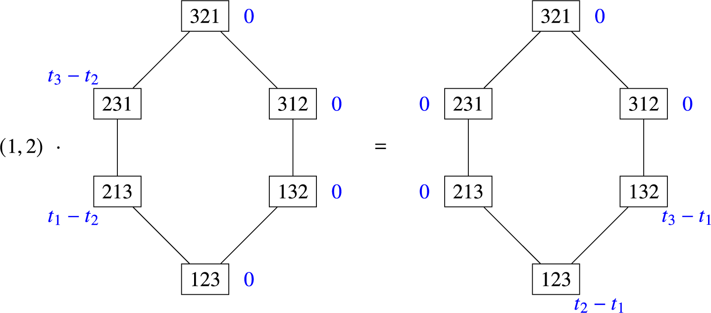
Example 2.13. The dot action of the transposition
 $(1,2)$
on the spline
$(1,2)$
on the spline
 $\bar {\rho }_3$
from Example 2.7 is computed below.
$\bar {\rho }_3$
from Example 2.7 is computed below.
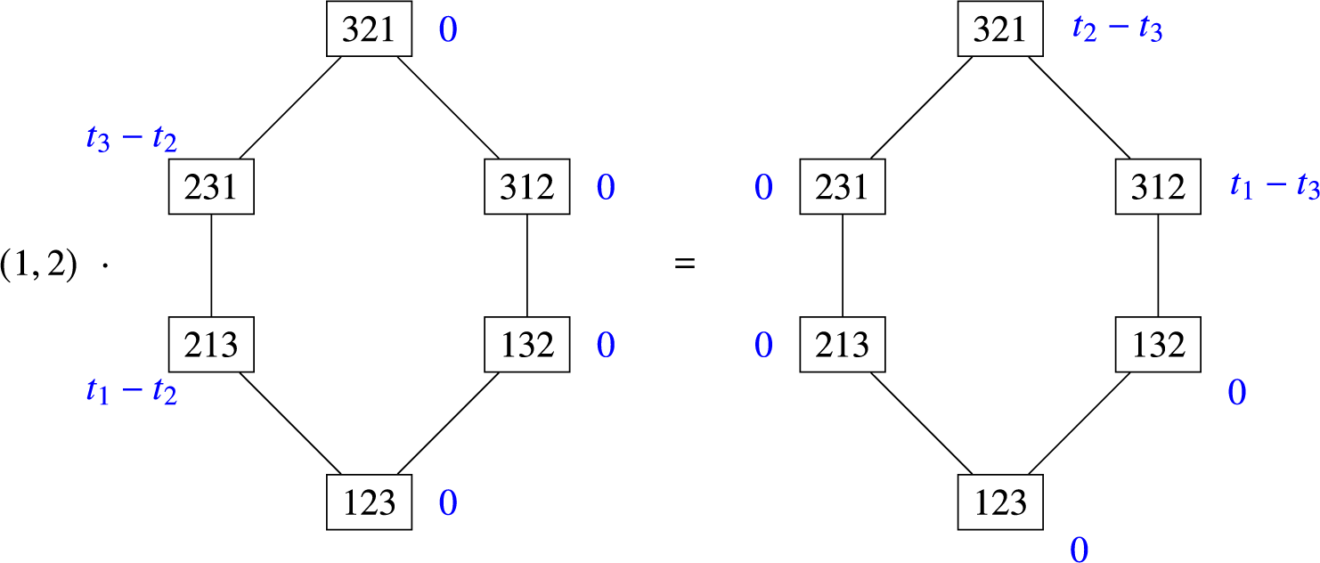
Computed below is the
 $\omega = (1,2,3)$
-twisted action of the transposition
$\omega = (1,2,3)$
-twisted action of the transposition
 $(1,2)$
on the spline
$(1,2)$
on the spline
 $\bar {\rho }_3$
from Example 2.7. Note this is the same as the untwisted action of
$\bar {\rho }_3$
from Example 2.7. Note this is the same as the untwisted action of
 $(1,2,3)(1,2)(1,2,3)^{-1} = (2,3)$
.
$(1,2,3)(1,2)(1,2,3)^{-1} = (2,3)$
.
Remark 2.14. The dot action is well defined. We have for all
 $(v_1,v_2) \in E(\mathcal {G}_\Gamma )$
that
$(v_1,v_2) \in E(\mathcal {G}_\Gamma )$
that
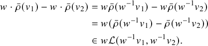 $$ \begin{align*} w \cdot \bar{\rho}(v_1) - w \cdot \bar{\rho}(v_2) &= w\bar{\rho}(w^{-1}v_1)- w\bar{\rho}(w^{-1}v_2) \\ &= w(\bar{\rho}(w^{-1}v_1)- \bar{\rho}(w^{-1}v_2)) \\ &\in w\mathcal{L}(w^{-1}v_1,w^{-1}v_2). \end{align*} $$
If
 $v_1v_2^{-1} = (i,j)$
, then
$v_1v_2^{-1} = (i,j)$
, then
 $w^{-1}v_1v_2^{-1}w = (w^{-1}(i),w^{-1}(j))$
. So
$w^{-1}v_1v_2^{-1}w = (w^{-1}(i),w^{-1}(j))$
. So
 $$\begin{align*}w\mathcal{L}(w^{-1}v_1,w^{-1}v_2) = \left\langle w(t_{w^{-1}(i)}-t_{w^{-1}(j)}) \right\rangle = \left\langle t_i-t_j \right\rangle = \mathcal{L}(v_1,v_2).\end{align*}$$
Thus,
 $w \cdot \bar {\rho }(v_1) - w \cdot \bar {\rho }(v_2) \in \mathcal {L}(v_1,v_2)$
, and
$w \cdot \bar {\rho }(v_1) - w \cdot \bar {\rho }(v_2) \in \mathcal {L}(v_1,v_2)$
, and
 $w \cdot \bar {\rho } \in \mathcal {M}_{\Gamma }$
.
$w \cdot \bar {\rho } \in \mathcal {M}_{\Gamma }$
.
Finally, consider the quotients
and
Call
 $\mathrm {L}_\Gamma $
and
$\mathrm {L}_\Gamma $
and
 $\mathrm {R}_\Gamma $
the left and right quotients of
$\mathrm {R}_\Gamma $
the left and right quotients of
 $\mathcal {M}_{\Gamma }$
, respectively. As
$\mathcal {M}_{\Gamma }$
, respectively. As
 $\mathbb {C}[t_\bullet ]$
-modules for the left and right action, both quotients are
$\mathbb {C}[t_\bullet ]$
-modules for the left and right action, both quotients are ![]() , where I is the ‘irrelevant ideal’
, where I is the ‘irrelevant ideal’
 $\left \langle t_1,...,t_n\right \rangle $
of
$\left \langle t_1,...,t_n\right \rangle $
of
 $\mathbb {C}[t_1,\ldots ,t_{n}]$
. Thus,
$\mathbb {C}[t_1,\ldots ,t_{n}]$
. Thus,
 $\mathrm {L}_{\Gamma }$
and
$\mathrm {L}_{\Gamma }$
and
 $\mathrm {R}_{\Gamma }$
each inherit the structure of a finite-dimensional graded
$\mathrm {R}_{\Gamma }$
each inherit the structure of a finite-dimensional graded
 $\mathbb {C}$
-vector space from the left- and right-module structure of
$\mathbb {C}$
-vector space from the left- and right-module structure of
 $\mathcal {M}_{\Gamma }$
, respectively. Any homogeneous module-generating set over
$\mathcal {M}_{\Gamma }$
, respectively. Any homogeneous module-generating set over
 $\mathbb {C}[t_\bullet ]$
projects to a spanning set over
$\mathbb {C}[t_\bullet ]$
projects to a spanning set over
 $\mathbb {C}$
in the quotient.
$\mathbb {C}$
in the quotient.
The ideals
 $\left \langle \bar {t}_1,\ldots ,\bar {t}_n\right \rangle $
and
$\left \langle \bar {t}_1,\ldots ,\bar {t}_n\right \rangle $
and
 $\left \langle \bar {x}_1,\ldots ,\bar {x}_n\right \rangle $
are homogeneous and
$\left \langle \bar {x}_1,\ldots ,\bar {x}_n\right \rangle $
are homogeneous and
 $S_n$
-equivariant, and so the graded
$S_n$
-equivariant, and so the graded
 $S_n$
-module structure on
$S_n$
-module structure on
 $\mathcal {M}_{\Gamma }$
projects to graded
$\mathcal {M}_{\Gamma }$
projects to graded
 $S_n$
-representations on both
$S_n$
-representations on both
 $\mathrm {L}_{\Gamma }$
and
$\mathrm {L}_{\Gamma }$
and
 $\mathrm {R}_{\Gamma }$
. Symmetric functions are formal power series in
$\mathrm {R}_{\Gamma }$
. Symmetric functions are formal power series in
 $\{x_1,x_2,...\}$
invariant under permuting the variables. The Frobenius character map gives an isomorphism from the algebra of representations of symmetric groups to the algebra of symmetric functions. The two bases of symmetric functions we consider are Schur functions
$\{x_1,x_2,...\}$
invariant under permuting the variables. The Frobenius character map gives an isomorphism from the algebra of representations of symmetric groups to the algebra of symmetric functions. The two bases of symmetric functions we consider are Schur functions
 $\{s_\lambda \}$
, which correspond to irreducible representations, and homogeneous symmetric functions {
$\{s_\lambda \}$
, which correspond to irreducible representations, and homogeneous symmetric functions {
 $h_\lambda \}$
, which correspond to induced representations of trivial representations on Young subgroups to symmetric groups. Both Schur and homogeneous symmetric functions are indexed by integer partitions. Denote the Frobenius character of these (q-graded)
$h_\lambda \}$
, which correspond to induced representations of trivial representations on Young subgroups to symmetric groups. Both Schur and homogeneous symmetric functions are indexed by integer partitions. Denote the Frobenius character of these (q-graded)
 $S_n$
-representations as
$S_n$
-representations as
 $\mathbf {ch}\left (\mathrm {L}_{\Gamma }\right )$
and
$\mathbf {ch}\left (\mathrm {L}_{\Gamma }\right )$
and
 $\mathbf {ch}\left (\mathrm {R}_{\Gamma }\right )$
, respectively. Since both
$\mathbf {ch}\left (\mathrm {R}_{\Gamma }\right )$
, respectively. Since both
 $\mathbf {ch}\left (\mathrm {L}_{\Gamma }\right )$
and
$\mathbf {ch}\left (\mathrm {L}_{\Gamma }\right )$
and
 $\mathbf {ch}\left (\mathrm {R}_{\Gamma }\right )$
correspond to graded representations, and all representations are sums of irreducible representations, both
$\mathbf {ch}\left (\mathrm {R}_{\Gamma }\right )$
correspond to graded representations, and all representations are sums of irreducible representations, both
 $\mathbf {ch}\left (\mathrm {L}_{\Gamma }\right )$
and
$\mathbf {ch}\left (\mathrm {L}_{\Gamma }\right )$
and
 $\mathbf {ch}\left (\mathrm {R}_{\Gamma }\right )$
are manifestly Schur-positive graded symmetric functions.
$\mathbf {ch}\left (\mathrm {R}_{\Gamma }\right )$
are manifestly Schur-positive graded symmetric functions.
Example 2.15. Again, consider
 $\Gamma = \left ([3],\{(1,2),(2,3)\}\right )$
. Then
$\Gamma = \left ([3],\{(1,2),(2,3)\}\right )$
. Then
 $$\begin{align*}\mathbf{ch}\left(\mathrm{L}_{\Gamma}\right) = s_3 + (s_{2,1} + 2s_3)q + s_3q^2=h_3 + (h_{2,1}+h_3)q + h_3q^2 \end{align*}$$
and
 $$\begin{align*}\mathbf{ch}\left(\mathrm{R}_{\Gamma}\right) = s_3 + 2s_{2,1}q + s_3q^2. \end{align*}$$
The following Lemma 2.16 is useful for computer calculations.
Lemma 2.16. Let
 $\Gamma $
and
$\Gamma $
and
 $\Gamma '$
be two graphs on
$\Gamma '$
be two graphs on
 $[n]$
, and
$[n]$
, and ![]() . Then
. Then
 $$\begin{align*}\mathcal{M}_{\Gamma \cup \Gamma'} = \mathcal{M}_{\Gamma} \cap \mathcal{M}_{\Gamma'} \end{align*}$$
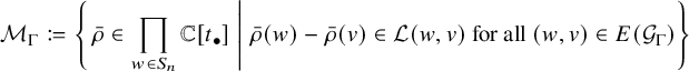
Proof. This easily follows from the set-theoretic definition
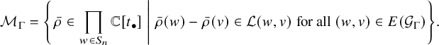 $$\begin{align*}\mathcal{M}_{\Gamma} = \left\{ \left.\bar{\rho} \in \prod_{w \in S_n} \mathbb{C}[t_\bullet]\; \right|\; \bar{\rho}(w) - \bar{\rho}(v) \in \mathcal{L}(w,v) \text{ for all } (w,v) \in E(\mathcal{G}_\Gamma)\right\}.\\[-48pt]\end{align*}$$
2.3 Isomorphisms
It is natural to expect that if two graphs
 $\Gamma $
and
$\Gamma $
and
 $\Gamma '$
on
$\Gamma '$
on
 $[n]$
are isomorphic, that the resulting algebraic structures on
$[n]$
are isomorphic, that the resulting algebraic structures on
 $\mathcal {M}_{\Gamma }$
and
$\mathcal {M}_{\Gamma }$
and
 $\mathcal {M}_{\Gamma '}$
should also have meaningful isomorphisms between them. This section shows that an isomorphism
$\mathcal {M}_{\Gamma '}$
should also have meaningful isomorphisms between them. This section shows that an isomorphism
 $\Gamma \to \Gamma '$
induces a labeled-graph isomorphism
$\Gamma \to \Gamma '$
induces a labeled-graph isomorphism
 $\mathcal {G}_\Gamma \to \mathcal {G}_{\Gamma '}$
, a ring isomorphism
$\mathcal {G}_\Gamma \to \mathcal {G}_{\Gamma '}$
, a ring isomorphism
 $\mathcal {M}_{\Gamma } \to \mathcal {M}_{\Gamma '}$
, a collection of different
$\mathcal {M}_{\Gamma } \to \mathcal {M}_{\Gamma '}$
, a collection of different
 $\mathbb {C}[t_\bullet ]$
-module isomorphisms
$\mathbb {C}[t_\bullet ]$
-module isomorphisms
 $\mathcal {M}_{\Gamma } \to \mathcal {M}_{\Gamma }$
, and an
$\mathcal {M}_{\Gamma } \to \mathcal {M}_{\Gamma }$
, and an
 $S_n$
-module isomorphism
$S_n$
-module isomorphism
 $\mathcal {M}_{\Gamma } \to \mathcal {M}_{\Gamma }$
that leads to equalities
$\mathcal {M}_{\Gamma } \to \mathcal {M}_{\Gamma }$
that leads to equalities
 $\mathbf {ch}\left (\mathrm {L}_{\Gamma }\right ) = \mathbf {ch}\left (\mathrm {L}_{\Gamma '}\right )$
and
$\mathbf {ch}\left (\mathrm {L}_{\Gamma }\right ) = \mathbf {ch}\left (\mathrm {L}_{\Gamma '}\right )$
and
 $\mathbf {ch}\left (\mathrm {R}_{\Gamma }\right ) = \mathbf {ch}\left (\mathrm {R}_{\Gamma '}\right )$
.
$\mathbf {ch}\left (\mathrm {R}_{\Gamma }\right ) = \mathbf {ch}\left (\mathrm {R}_{\Gamma '}\right )$
.
Throughout this subsection, let
 $\Gamma $
and
$\Gamma $
and
 $\Gamma '$
be graphs on
$\Gamma '$
be graphs on
 $[n]$
and say that
$[n]$
and say that
 $\omega \colon \Gamma \to \Gamma '$
is a graph isomorphism. Then
$\omega \colon \Gamma \to \Gamma '$
is a graph isomorphism. Then
 $\omega $
is also naturally an element of
$\omega $
is also naturally an element of
 $S_n$
, viewed as a bijection from
$S_n$
, viewed as a bijection from
 $[n]$
to itself. Let
$[n]$
to itself. Let
 $\omega $
denote both the graph isomorphism and associated permutation.
$\omega $
denote both the graph isomorphism and associated permutation.
Our first construction is an isomorphism between the corresponding labeled Cayley graphs. The following Lemma 2.17 states that
 $\mathcal {G}_\Gamma $
and
$\mathcal {G}_\Gamma $
and
 $\mathcal {G}_{\Gamma '}$
are related as graphs by conjugation, and the associated labels are related via the action on ideals induced by the action on polynomials in Equation (2.1).
$\mathcal {G}_{\Gamma '}$
are related as graphs by conjugation, and the associated labels are related via the action on ideals induced by the action on polynomials in Equation (2.1).
Lemma 2.17. Let
 $\omega \colon \Gamma \to \Gamma '$
be a graph isomorphism. Then
$\omega \colon \Gamma \to \Gamma '$
be a graph isomorphism. Then
 $v \mapsto \omega v \omega ^{-1}$
is a graph isomorphism
$v \mapsto \omega v \omega ^{-1}$
is a graph isomorphism
 $\mathcal {G}_\Gamma \to \mathcal {G}_{\Gamma '}$
. Additionally, if
$\mathcal {G}_\Gamma \to \mathcal {G}_{\Gamma '}$
. Additionally, if
 $\mathcal {L}$
is the label on
$\mathcal {L}$
is the label on
 $\mathcal {G}_{\Gamma }$
,
$\mathcal {G}_{\Gamma }$
,
 $\mathcal {L'}$
the label on
$\mathcal {L'}$
the label on
 $\mathcal {G}_{\Gamma '}$
, and
$\mathcal {G}_{\Gamma '}$
, and
 $(v_1,v_2) \in E(\mathcal {G}_\Gamma )$
, then
$(v_1,v_2) \in E(\mathcal {G}_\Gamma )$
, then
 $\mathcal {L}'(\omega v_1 \omega ^{-1},\omega v_2 \omega ^{-1}) = \omega \mathcal {L}(v_1,v_2)$
.
$\mathcal {L}'(\omega v_1 \omega ^{-1},\omega v_2 \omega ^{-1}) = \omega \mathcal {L}(v_1,v_2)$
.
Proof. Conjugation is a group automorphism of
 $S_n$
. Say
$S_n$
. Say
 $(v_1,v_2) \in E(\Gamma )$
and in particular that
$(v_1,v_2) \in E(\Gamma )$
and in particular that
 $v_1^{-1}v_2 = (i,j) \in E(\Gamma )$
. Then
$v_1^{-1}v_2 = (i,j) \in E(\Gamma )$
. Then
 $$ \begin{align*} \left(\omega v_1 \omega^{-1}\right)^{-1}\left(\omega v_2\omega^{-1}\right) &= \omega v_1^{-1} v_2\omega^{-1} \\ &= \omega(i,j)\omega^{-1} \\ &= \left(\omega(i),\omega(j)\right) \in E(\Gamma'). \end{align*} $$
Thus, conjugation by
 $\omega $
defines a graph isomorphism
$\omega $
defines a graph isomorphism
 $\mathcal {G}_\Gamma \to \mathcal {G}_{\Gamma '}$
. For the labels on
$\mathcal {G}_\Gamma \to \mathcal {G}_{\Gamma '}$
. For the labels on
 $\mathcal {G}_\Gamma $
and
$\mathcal {G}_\Gamma $
and
 $\mathcal {G}_{\Gamma '}$
, the computation above also shows that if
$\mathcal {G}_{\Gamma '}$
, the computation above also shows that if
 $v_1v_2^{-1} = (p,q)$
, then
$v_1v_2^{-1} = (p,q)$
, then
 $\left (\omega v_1 \omega ^{-1}\right )\left (\omega v_2\omega ^{-1}\right )^{-1} = (\omega (p),\omega (q))$
. It follows that
$\left (\omega v_1 \omega ^{-1}\right )\left (\omega v_2\omega ^{-1}\right )^{-1} = (\omega (p),\omega (q))$
. It follows that
 $\left (\omega v_1 \omega ^{-1},\omega v_2\omega ^{-1}\right ) \in E(\mathcal {G}_{\Gamma '})$
is labeled
$\left (\omega v_1 \omega ^{-1},\omega v_2\omega ^{-1}\right ) \in E(\mathcal {G}_{\Gamma '})$
is labeled
 $\left \langle t_{\omega (p)} - t_{\omega (q)}\right \rangle = \omega \left \langle t_p-t_q\right \rangle $
. The claim follows.
$\left \langle t_{\omega (p)} - t_{\omega (q)}\right \rangle = \omega \left \langle t_p-t_q\right \rangle $
. The claim follows.
Define
 $\Omega \colon \mathcal {M}_{\Gamma } \to \mathcal {M}_{\Gamma '}$
by
$\Omega \colon \mathcal {M}_{\Gamma } \to \mathcal {M}_{\Gamma '}$
by ![]() . The following Proposition 2.18 proves
. The following Proposition 2.18 proves
 $\Omega $
is a ring isomorphism and is actually a consequence of Lemma 2.17 and a more general Proposition of Gilbert, Tymoczko and Viel [Reference Gilbert, Tymoczko and Viel15, Prop 2.7]. We include the proof here for completeness.
$\Omega $
is a ring isomorphism and is actually a consequence of Lemma 2.17 and a more general Proposition of Gilbert, Tymoczko and Viel [Reference Gilbert, Tymoczko and Viel15, Prop 2.7]. We include the proof here for completeness.
Proposition 2.18. The map
 $\Omega \colon \mathcal {M}_{\Gamma } \to \mathcal {M}_{\Gamma '}$
is a ring isomorphism.
$\Omega \colon \mathcal {M}_{\Gamma } \to \mathcal {M}_{\Gamma '}$
is a ring isomorphism.
Proof. Let
 $\bar {\rho } \in \mathcal {M}_{\Gamma }$
. First, we show that
$\bar {\rho } \in \mathcal {M}_{\Gamma }$
. First, we show that
 $\Omega (\bar {\rho }) \in \mathcal {M}_{\Gamma '}$
. Let
$\Omega (\bar {\rho }) \in \mathcal {M}_{\Gamma '}$
. Let
 $(v_1,v_2) \in E(\mathcal {G}_{\Gamma '})$
. By Lemma 2.17, there is an edge
$(v_1,v_2) \in E(\mathcal {G}_{\Gamma '})$
. By Lemma 2.17, there is an edge
 $(\omega ^{-1}v_1\omega ,\omega ^{-1}v_2\omega ) \in E(\mathcal {G}_\Gamma )$
, and so
$(\omega ^{-1}v_1\omega ,\omega ^{-1}v_2\omega ) \in E(\mathcal {G}_\Gamma )$
, and so
 $\bar {\rho }(\omega ^{-1}v_1\omega )-\bar {\rho }(\omega ^{-1}v_2\omega ) \in \mathcal {L}(\omega ^{-1}v_1\omega ,\omega ^{-1}v_2\omega )$
. Now we have
$\bar {\rho }(\omega ^{-1}v_1\omega )-\bar {\rho }(\omega ^{-1}v_2\omega ) \in \mathcal {L}(\omega ^{-1}v_1\omega ,\omega ^{-1}v_2\omega )$
. Now we have
 $$ \begin{align*} \Omega(\bar{\rho})(v_1) - \Omega(\bar{\rho})(v_2) &= \omega\bar{\rho}\left(\omega^{-1} v_1 \omega\right) - \omega\bar{\rho}\left(\omega^{-1} v_2 \omega\right) \\ &= \omega\left(\bar{\rho}\left(\omega^{-1} v_1 \omega\right) - \bar{\rho}\left(\omega^{-1} v_2 \omega\right)\right) \\ &\in \omega \mathcal{L}\left(\omega^{-1} v_1 \omega,\omega^{-1} v_2 \omega\right) = \mathcal{L}'(v_1,v_2). \end{align*} $$
Thus,
 $\Omega (\bar {\rho }) \in \mathcal {M}_{\Gamma '}$
. It is easy to verify that this map is a ring homomorphism, and the inverse from
$\Omega (\bar {\rho }) \in \mathcal {M}_{\Gamma '}$
. It is easy to verify that this map is a ring homomorphism, and the inverse from
 $\mathcal {M}_{\Gamma '}$
to
$\mathcal {M}_{\Gamma '}$
to
 $\mathcal {M}_{\Gamma }$
is constructed in the same manner with the map
$\mathcal {M}_{\Gamma }$
is constructed in the same manner with the map
 $\omega ^{-1} \colon \Gamma ' \to \Gamma $
.
$\omega ^{-1} \colon \Gamma ' \to \Gamma $
.
The following lemma gives three instances in which
 $\Omega $
is also a module isomorphism between
$\Omega $
is also a module isomorphism between
 $\mathcal {M}_{\Gamma }$
and
$\mathcal {M}_{\Gamma }$
and
 $\mathcal {M}_{\Gamma '}$
.
$\mathcal {M}_{\Gamma '}$
.
Lemma 2.19. The ring isomorphism
 $\Omega $
is a module isomorphism from
$\Omega $
is a module isomorphism from
 $\mathcal {M}_{\Gamma }$
to
$\mathcal {M}_{\Gamma }$
to
 $\mathcal {M}_{\Gamma '}$
with respect to the following actions:
$\mathcal {M}_{\Gamma '}$
with respect to the following actions:
-
1. the left
$\mathbb {C}[t_\bullet ]$
-action on
$\mathcal {M}_{\Gamma }$
to the
$\omega $
-twisted left
$\mathbb {C}[t_\bullet ]$
-action on
$\mathcal {M}_{\Gamma '}$
, -
2. the right
$\mathbb {C}[t_\bullet ]$
-action on
$\mathcal {M}_{\Gamma }$
to the
$\omega $
-twisted right
$\mathbb {C}[t_\bullet ]$
-action on
$\mathcal {M}_{\Gamma '}$
, and -
3. the dot action of
$S_n$
on
$\mathcal {M}_{\Gamma }$
to the
$\omega $
-twisted dot action of
$S_n$
on
$\mathcal {M}_{\Gamma '}$
.


Proof. Both
 $\mathbb {C}[t_\bullet ]$
-module statements follow from two straightforward computations,
$\mathbb {C}[t_\bullet ]$
-module statements follow from two straightforward computations,
 $$\begin{align*}\Omega(\bar{t}_i)(v) =\bar{t}_{\omega(i)}(v)\; \text{ and }\; \Omega(\bar{x}_i)(v) = \bar{x}_{\omega(i)}(v). \end{align*}$$
Say for the left action, if
 $f \in \mathbb {C}[t_\bullet ]$
and
$f \in \mathbb {C}[t_\bullet ]$
and
 $\bar {\rho } \in \mathcal {M}_{\Gamma }$
, then
$\bar {\rho } \in \mathcal {M}_{\Gamma }$
, then
 $\Omega (f(t_1,\ldots ,t_n).\bar {\rho }) = f(\bar {t}_{\omega (1)},\ldots ,\bar {t}_{\omega (n)})\Omega (\bar {\rho })$
, precisely the twisted action. The same holds for the right
$\Omega (f(t_1,\ldots ,t_n).\bar {\rho }) = f(\bar {t}_{\omega (1)},\ldots ,\bar {t}_{\omega (n)})\Omega (\bar {\rho })$
, precisely the twisted action. The same holds for the right
 $\mathbb {C}[t_\bullet ]$
-action to the
$\mathbb {C}[t_\bullet ]$
-action to the
 $\omega $
-twisted right
$\omega $
-twisted right
 $\mathbb {C}[t_\bullet ]$
-action. It is easy to show that ring isomorphism
$\mathbb {C}[t_\bullet ]$
-action. It is easy to show that ring isomorphism
 $\Omega ^{-1}$
is the inverse for
$\Omega ^{-1}$
is the inverse for
 $\Omega $
as a
$\Omega $
as a
 $\mathbb {C}[t_\bullet ]$
-module morphism for both pairs of actions, and so
$\mathbb {C}[t_\bullet ]$
-module morphism for both pairs of actions, and so
 $\Omega $
is a
$\Omega $
is a
 $\mathbb {C}[t_\bullet ]$
-module isomorphism as in (1) and (2).
$\mathbb {C}[t_\bullet ]$
-module isomorphism as in (1) and (2).
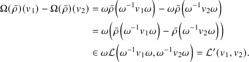
Given the dot action on
 $\mathcal {M}_{\Gamma }$
, the induced action of
$\mathcal {M}_{\Gamma }$
, the induced action of
 $u \in S_n$
on
$u \in S_n$
on
 $\bar {\rho } \in \mathcal {M}_{\Gamma '}$
is
$\bar {\rho } \in \mathcal {M}_{\Gamma '}$
is
To check that the action is compatible with multiplication of elements
 $v,u \in S_n$
, compute
$v,u \in S_n$
, compute
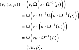 $$ \begin{align*} (v,(u,\bar{\rho})) &= \left(v,\Omega\left( u \cdot \Omega^{-1}(\bar{\rho})\right)\right) \\ &= \Omega\left( v \cdot \Omega^{-1}\Omega\left( u \cdot \Omega^{-1}(\bar{\rho})\right)\right) \\ &= \Omega\left( v \cdot \left( u \cdot \Omega^{-1}(\bar{\rho})\right)\right)\\ &= \Omega\left( vu \cdot \Omega^{-1}(\bar{\rho})\right)\\ &= (vu,\bar{\rho}). \end{align*} $$
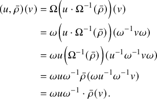
Now compute for
 $u,v \in S_n$
that
$u,v \in S_n$
that
 $$ \begin{align*} (u,\bar{\rho})(v) &= \Omega\left( u \cdot \Omega^{-1}(\bar{\rho})\right) (v) \\ &= \omega \left( u\cdot \Omega^{-1}(\bar{\rho})\right)(\omega^{-1}v\omega) \\ &= \omega u \left(\Omega^{-1}(\bar{\rho})\right)(u^{-1}\omega^{-1}v\omega) \\ &= \omega u \omega^{-1}\bar{\rho}(\omega u^{-1}\omega^{-1}v)\\ &= \omega u \omega^{-1} \cdot \bar{\rho}(v). \end{align*} $$
This is precisely the
 $\omega $
-twisted dot action of u on
$\omega $
-twisted dot action of u on
 $\mathcal {M}_{\Gamma '}$
. Again, by computing with
$\mathcal {M}_{\Gamma '}$
. Again, by computing with
 $\Omega ^{-1}$
, it follows that
$\Omega ^{-1}$
, it follows that
 $\Omega $
is an
$\Omega $
is an
 $S_n$
-module isomorphism.
$S_n$
-module isomorphism.
Note that any generating set for the left or right
 $\mathbb {C}[t_\bullet ]$
-module structures on
$\mathbb {C}[t_\bullet ]$
-module structures on
 $\mathcal {M}_{\Gamma }$
must necessarily be generators for the
$\mathcal {M}_{\Gamma }$
must necessarily be generators for the
 $\omega $
-twisted versions as well. As such, when searching for generators, we may choose any graph isomorphic to
$\omega $
-twisted versions as well. As such, when searching for generators, we may choose any graph isomorphic to
 $\Gamma $
for explicit calculations.
$\Gamma $
for explicit calculations.
Proposition 2.20. If
 $\Gamma $
and
$\Gamma $
and
 $\Gamma '$
are isomorphic, then
$\Gamma '$
are isomorphic, then
 $\mathbf {ch}\left (\mathrm {L}_{\Gamma }\right ) =\mathbf {ch}\left (\mathrm {L}_{\Gamma '}\right )$
and
$\mathbf {ch}\left (\mathrm {L}_{\Gamma }\right ) =\mathbf {ch}\left (\mathrm {L}_{\Gamma '}\right )$
and
 $\mathbf {ch}\left (\mathrm {R}_{\Gamma }\right ) = \mathbf {ch}\left (\mathrm {R}_{\Gamma '}\right )$
.
$\mathbf {ch}\left (\mathrm {R}_{\Gamma }\right ) = \mathbf {ch}\left (\mathrm {R}_{\Gamma '}\right )$
.
Proof. Let
 $\omega $
be an isomorphism from
$\omega $
be an isomorphism from
 $\Gamma $
to
$\Gamma $
to
 $\Gamma '$
. The
$\Gamma '$
. The
 $S_n$
-isomorphism
$S_n$
-isomorphism
 $\Omega $
from Lemma 2.19 (3) preserves the ideal
$\Omega $
from Lemma 2.19 (3) preserves the ideal
 $\left \langle \bar {t}_1,\ldots ,\bar {t}_n\right \rangle $
from
$\left \langle \bar {t}_1,\ldots ,\bar {t}_n\right \rangle $
from
 $\mathcal {M}_{\Gamma }$
to
$\mathcal {M}_{\Gamma }$
to
 $\mathcal {M}_{\Gamma '}$
. Thus, we have a
$\mathcal {M}_{\Gamma '}$
. Thus, we have a
 $S_n$
-module isomorphism from
$S_n$
-module isomorphism from
 $\mathrm {L}_{\Gamma }$
to the
$\mathrm {L}_{\Gamma }$
to the
 $\omega $
-twisted
$\omega $
-twisted
 $\mathrm {L}_{\Gamma '}$
. Twisting by
$\mathrm {L}_{\Gamma '}$
. Twisting by
 $\omega $
is an inner automorphism of
$\omega $
is an inner automorphism of
 $S_n$
, so the
$S_n$
, so the
 $\omega $
-twisted
$\omega $
-twisted
 $\mathrm {L}_{\Gamma '}$
is in turn isomorphic to the untwisted
$\mathrm {L}_{\Gamma '}$
is in turn isomorphic to the untwisted
 $\mathrm {L}_{\Gamma '}$
as an
$\mathrm {L}_{\Gamma '}$
as an
 $S_n$
-representation. The exact same argument holds for
$S_n$
-representation. The exact same argument holds for
 $\mathrm {R}_{\Gamma }$
and
$\mathrm {R}_{\Gamma }$
and
 $\mathrm {R}_{\Gamma '}$
. Isomorphic representations have identical traces (i.e., equal characters), and the equalities follow.
$\mathrm {R}_{\Gamma '}$
. Isomorphic representations have identical traces (i.e., equal characters), and the equalities follow.
By Proposition 2.20, we may consider any graph isomorphic to
 $\Gamma $
when calculating
$\Gamma $
when calculating
 $\mathbf {ch}\left (\mathrm {L}_{\Gamma }\right )$
and
$\mathbf {ch}\left (\mathrm {L}_{\Gamma }\right )$
and
 $\mathbf {ch}\left (\mathrm {R}_{\Gamma }\right )$
.
$\mathbf {ch}\left (\mathrm {R}_{\Gamma }\right )$
.
Corollary 2.21. The graded symmetric functions
 $\mathbf {ch}\left (\mathrm {L}_{\Gamma }\right )$
and
$\mathbf {ch}\left (\mathrm {L}_{\Gamma }\right )$
and
 $\mathbf {ch}\left (\mathrm {R}_{\Gamma }\right )$
are invariants of simple graphs.
$\mathbf {ch}\left (\mathrm {R}_{\Gamma }\right )$
are invariants of simple graphs.
3 Module structure of
$\mathcal {M}_{\Gamma }$

This section establishes some algebraic properties of
 $\mathcal {M}_{\Gamma }$
as a module over the polynomial ring
$\mathcal {M}_{\Gamma }$
as a module over the polynomial ring
 $\mathbb {C}[t_\bullet ]$
. It begins with two results: one that establishes the size of a minimal homogeneous
$\mathbb {C}[t_\bullet ]$
. It begins with two results: one that establishes the size of a minimal homogeneous
 $\mathbb {C}[t_\bullet ]$
-module generating set as an invariant of
$\mathbb {C}[t_\bullet ]$
-module generating set as an invariant of
 $\Gamma $
and a second that proves the module generated by constant and linear splines is a free module over
$\Gamma $
and a second that proves the module generated by constant and linear splines is a free module over
 $\mathbb {C}[t_\bullet ]$
. This section continues with subsection 3.1, which establishes an algebraic relation that must be satisfied by elements of
$\mathbb {C}[t_\bullet ]$
. This section continues with subsection 3.1, which establishes an algebraic relation that must be satisfied by elements of
 $\mathcal {M}_{\Gamma }$
. This section ends with subsection 3.2, which gives an explicit and combinatorially meaningful generating set of
$\mathcal {M}_{\Gamma }$
. This section ends with subsection 3.2, which gives an explicit and combinatorially meaningful generating set of
 $\mathcal {M}_{\Gamma }$
as a
$\mathcal {M}_{\Gamma }$
as a
 $\mathbb {C}[t_\bullet ]$
-module when
$\mathbb {C}[t_\bullet ]$
-module when
 $\Gamma $
is a tree (proving Theorem 1.2).
$\Gamma $
is a tree (proving Theorem 1.2).
Before continuing, we will briefly describe what is already known in the geometric case. If
 $\Gamma $
is a Hessenberg graph, then
$\Gamma $
is a Hessenberg graph, then
-
•
$\mathcal {M}_{\Gamma }$
is a free
$\mathbb {C}[t_\bullet ]$
-module with a combinatorial formula for its rank-generating function [Reference De Mari, Procesi and Shayman13], and furthermore, -
•
$\mathcal {M}_{\Gamma }$
has explicit upper-triangular generators are achieved from a Białynicki-Birula decomposition of the corresponding variety [Reference Cho, Hong and Lee9, Reference De Mari, Procesi and Shayman13].


In the geometric case, the rank-generating function is equivalent (substituting
 $q \mapsto q^2$
) to the Poincaré polynomial of the corresponding variety. If
$q \mapsto q^2$
) to the Poincaré polynomial of the corresponding variety. If
 $\Gamma $
is not in the geometric case, then
$\Gamma $
is not in the geometric case, then
 $\mathcal {M}_{\Gamma }$
is not always a free module. We now prove that the number of generators in each degree of a homogeneous generating set is still an invariant of
$\mathcal {M}_{\Gamma }$
is not always a free module. We now prove that the number of generators in each degree of a homogeneous generating set is still an invariant of
 $\Gamma $
. We compute the minimal number of linear generators for
$\Gamma $
. We compute the minimal number of linear generators for
 $\mathcal {M}_{\Gamma }$
in Section 8.
$\mathcal {M}_{\Gamma }$
in Section 8.
A generating set F of a finitely generated
 $\mathbb {C}[t_\bullet ]$
-module M is minimal if there exists a collection of polynomials
$\mathbb {C}[t_\bullet ]$
-module M is minimal if there exists a collection of polynomials
 $\{c_f \mid f \in F\} \subset \mathbb {C}[t_\bullet ]$
such that
$\{c_f \mid f \in F\} \subset \mathbb {C}[t_\bullet ]$
such that
 $\sum _{f \in F} c_f.f = 0$
. Then
$\sum _{f \in F} c_f.f = 0$
. Then
 $c_f \notin \mathbb {C} \setminus \{0\}$
for all
$c_f \notin \mathbb {C} \setminus \{0\}$
for all
 $f \in F$
(i.e., no
$f \in F$
(i.e., no
 $c_f$
is a unit). In other words, no proper subset of F generates M. If M is graded, then a set F is homogeneous if every element
$c_f$
is a unit). In other words, no proper subset of F generates M. If M is graded, then a set F is homogeneous if every element
 $f \in F$
is homogeneous.
$f \in F$
is homogeneous.
The following lemma is known, essentially as a corollary to the graded Nakayama lemma, and holds in greater generality (i.e., for other graded rings over a field). We include a proof for completeness.
Lemma 3.1. Let M be a finitely generated
 $\mathbb { N}$
-graded module over
$\mathbb { N}$
-graded module over
 $\mathbb {C}[t_\bullet ]$
. Then every minimal homogeneous generating set has the same number of elements of each degree.
$\mathbb {C}[t_\bullet ]$
. Then every minimal homogeneous generating set has the same number of elements of each degree.
Proof. Let
 $I = \left \langle t_\bullet \right \rangle $
be the irrelevant ideal. As
$I = \left \langle t_\bullet \right \rangle $
be the irrelevant ideal. As ![]() , the quotient
, the quotient ![]() is a graded
is a graded
 $\mathbb {C}$
-module. In particular,
$\mathbb {C}$
-module. In particular, ![]() is a graded
is a graded
 $\mathbb {C}$
-vector space of dimension
$\mathbb {C}$
-vector space of dimension
 $(d_0,\ldots ,d_n)$
, and we will prove that any homogeneous minimal generating set for M projects to a graded basis in
$(d_0,\ldots ,d_n)$
, and we will prove that any homogeneous minimal generating set for M projects to a graded basis in ![]() . Let
. Let ![]() be a minimal homogeneous generating set of M with
be a minimal homogeneous generating set of M with
 $K_i$
elements of degree i. It is easy to reason that
$K_i$
elements of degree i. It is easy to reason that
 $n=N$
since an element in M of degree greater than N is in
$n=N$
since an element in M of degree greater than N is in
 $IF = IM$
(so
$IF = IM$
(so
 $n \leq N$
), and if
$n \leq N$
), and if
 $f_1^N \in IM$
, then F is not minimal (so
$f_1^N \in IM$
, then F is not minimal (so
 $n \geq N$
). In fact, if
$n \geq N$
). In fact, if
 $f \in F$
and
$f \in F$
and
 $f \in IM$
, then F is not minimal (f would be in the
$f \in IM$
, then F is not minimal (f would be in the
 $\mathbb {C}[t_\bullet ]$
-span of lower degree elements of F), and moreover, since we are assuming that F is minimal, we know that the image of
$\mathbb {C}[t_\bullet ]$
-span of lower degree elements of F), and moreover, since we are assuming that F is minimal, we know that the image of
 $f \in F$
in
$f \in F$
in ![]() is nonzero. We will show that
is nonzero. We will show that
 $K_i = d_i$
for all
$K_i = d_i$
for all
 $i=1,...,N$
. Let
$i=1,...,N$
. Let ![]() be the quotient map.
be the quotient map.
We know
 $\pi (F)$
is a homogeneous spanning set for the graded vector space
$\pi (F)$
is a homogeneous spanning set for the graded vector space ![]() . Since
. Since ![]() is a graded vector space, we may prove linear independence degree-by-degree. Say for
is a graded vector space, we may prove linear independence degree-by-degree. Say for
 $c_1,\ldots ,c_{K_i} \in \mathbb {C}$
that
$c_1,\ldots ,c_{K_i} \in \mathbb {C}$
that
 ${ \sum\limits _{k=1}^{K_i} c_k\pi (f_k^i) = 0}$
. We will show that
${ \sum\limits _{k=1}^{K_i} c_k\pi (f_k^i) = 0}$
. We will show that
 $c_1 = \cdots = c_{K_i} = 0$
. It follows that
$c_1 = \cdots = c_{K_i} = 0$
. It follows that
 ${ \pi \left ( \sum\limits_{k=1}^{K_i} c_kf_k^i\right )} = 0$
, and so
${ \pi \left ( \sum\limits_{k=1}^{K_i} c_kf_k^i\right )} = 0$
, and so
 ${ \sum\limits_{k=1}^{K_i} c_kf_k^i \in IM}$
. So there exists some finite set P that indexes two subsets
${ \sum\limits_{k=1}^{K_i} c_kf_k^i \in IM}$
. So there exists some finite set P that indexes two subsets
 $\{r_p \mid p \in P\} \subset I$
and
$\{r_p \mid p \in P\} \subset I$
and
 $\{h_p \mid P \in P\} \subset M$
such that
$\{h_p \mid P \in P\} \subset M$
such that
 ${ \sum\limits_{k=1}^{K_i} c_kf_k^i = \sum _{p \in P}r_p.h_p}$
. Since
${ \sum\limits_{k=1}^{K_i} c_kf_k^i = \sum _{p \in P}r_p.h_p}$
. Since
 ${ \sum\limits_{k=1}^{K_i} c_kf_k^i}$
is homogeneous of degree i, it suffices to consider only the i-th graded piece of each element
${ \sum\limits_{k=1}^{K_i} c_kf_k^i}$
is homogeneous of degree i, it suffices to consider only the i-th graded piece of each element
 $r_ph_p$
.
$r_ph_p$
.
Say
 $i=0$
. Since each
$i=0$
. Since each
 $r_p \in I$
has no degree
$r_p \in I$
has no degree
 $0$
component, neither does
$0$
component, neither does
 $r_ph_p$
, so
$r_ph_p$
, so
 ${ \sum\limits _{k=1}^{K_0} c_kf_k^0 = 0}$
. Since F is a minimal generating set for M, it follows that
${ \sum\limits _{k=1}^{K_0} c_kf_k^0 = 0}$
. Since F is a minimal generating set for M, it follows that
 $c_1=\cdots =c_{k_0} = 0$
.
$c_1=\cdots =c_{k_0} = 0$
.
Now say
 $i>0$
. Each
$i>0$
. Each
 $h_p$
is degree at most
$h_p$
is degree at most
 $i-1$
, so
$i-1$
, so
 $\sum _{ p \in P} r_p.h_p \in \mathbb {C}[t_\bullet ]\{f_q^j \mid 0\leq j < i,\; q \in [K_j]\}$
. So
$\sum _{ p \in P} r_p.h_p \in \mathbb {C}[t_\bullet ]\{f_q^j \mid 0\leq j < i,\; q \in [K_j]\}$
. So
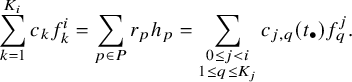 $$\begin{align*}\sum_{k=1}^{K_i} c_kf_k^i = \sum_{p \in P} r_ph_p = \sum_{\substack{0\leq j < i\\ 1\leq q \leq K_j}} c_{j,q}(t_\bullet) f_q^j.\end{align*}$$
This is a relation in M of elements from F and thus cannot have any nonzero constant coefficients, so
 $c_1 = \cdots =c_{k_i} = 0$
. Thus,
$c_1 = \cdots =c_{k_i} = 0$
. Thus,
 $\{\pi (f_k^i) \mid k \in [K_i]\}$
is a basis of the i-th graded piece of the vector space
$\{\pi (f_k^i) \mid k \in [K_i]\}$
is a basis of the i-th graded piece of the vector space ![]() , and so
, and so
 $K_i = d_i$
is independent of the choice of F.
$K_i = d_i$
is independent of the choice of F.
The proof of Lemma 3.1 also ensures that a minimal graded generating set of
 $\mathcal {M}_{\Gamma }$
with respect to either the left or right module structure projects to a basis of
$\mathcal {M}_{\Gamma }$
with respect to either the left or right module structure projects to a basis of
 $\mathrm {L}_{\Gamma }$
or
$\mathrm {L}_{\Gamma }$
or
 $\mathrm {R}_{\Gamma }$
, respectively.
$\mathrm {R}_{\Gamma }$
, respectively.
Lemma 3.2 below shows that the first graded piece of the
 $\mathbb {C}[t_\bullet ]$
-module is free. Note Lemma 3.2 is independent of the polynomial action chosen (e.g., left, right, and twisted alternatives).
$\mathbb {C}[t_\bullet ]$
-module is free. Note Lemma 3.2 is independent of the polynomial action chosen (e.g., left, right, and twisted alternatives).
Lemma 3.2. The
 $\mathbb {C}[t_\bullet ]$
-submodule
$\mathbb {C}[t_\bullet ]$
-submodule
 $\mathcal {M}_{\Gamma }^{\leq 1}$
generated by the constant and linear splines on
$\mathcal {M}_{\Gamma }^{\leq 1}$
generated by the constant and linear splines on
 $\mathcal {G}_\Gamma $
is a free module.
$\mathcal {G}_\Gamma $
is a free module.
Proof. Let
 $(e,w_2,w_3,\ldots ,w_{n!})$
be a linear order on
$(e,w_2,w_3,\ldots ,w_{n!})$
be a linear order on
 $S_n$
, where
$S_n$
, where
 $\ell _\Gamma (v) < \ell _\Gamma (w)$
implies that
$\ell _\Gamma (v) < \ell _\Gamma (w)$
implies that
 $v<w$
. Since
$v<w$
. Since
 $\Gamma $
is connected, if
$\Gamma $
is connected, if
 $w \neq e$
, there exists
$w \neq e$
, there exists
 $(i,j) \in E(\Gamma )$
such that
$(i,j) \in E(\Gamma )$
such that
 $w(i,j) < w$
.
$w(i,j) < w$
.
Let ![]() be a minimal generating set of
be a minimal generating set of
 $\mathcal {M}_{\Gamma }^{\leq 1}$
, where each
$\mathcal {M}_{\Gamma }^{\leq 1}$
, where each
 $\bar {f}_1,\ldots ,\bar {f}_k$
is a linear spline. Then
$\bar {f}_1,\ldots ,\bar {f}_k$
is a linear spline. Then ![]() is a homogeneous generating set of the same size and is therefore minimal by Lemma 3.1. This new generating set has the property that the
is a homogeneous generating set of the same size and is therefore minimal by Lemma 3.1. This new generating set has the property that the ![]() is the unique spline whose minimal element is e, so assume that
is the unique spline whose minimal element is e, so assume that
 $\bar {f}(e) = 0$
for all
$\bar {f}(e) = 0$
for all ![]() .
.
Let ![]() . So
. So ![]() . We iteratively construct a minimal generating set such that
. We iteratively construct a minimal generating set such that
 $\left | F_v \right | \in \{0,1\}$
for all
$\left | F_v \right | \in \{0,1\}$
for all
 $v \in S_n$
. Say that
$v \in S_n$
. Say that
 $\left | F_v \right | \in \{0,1\}$
for all
$\left | F_v \right | \in \{0,1\}$
for all
 $v < w$
, and
$v < w$
, and
 $\left | F_w \right | \geq 2$
. Let
$\left | F_w \right | \geq 2$
. Let
 $F_w = \{\bar {g}_1,\ldots ,\bar {g}_r\}$
. Since the linear order on
$F_w = \{\bar {g}_1,\ldots ,\bar {g}_r\}$
. Since the linear order on
 $S_n$
is an extension of
$S_n$
is an extension of
 $\Gamma $
-length, there exists
$\Gamma $
-length, there exists
 $(a,b) \in E(\Gamma )$
such that
$(a,b) \in E(\Gamma )$
such that
 $w(a,b) < w$
, and so
$w(a,b) < w$
, and so
 $\bar {g}(w(a,b)) = 0$
for all
$\bar {g}(w(a,b)) = 0$
for all
 $\bar {g} \in F_w$
. Thus, there exist
$\bar {g} \in F_w$
. Thus, there exist
 $c_1,\ldots ,c_r \in \mathbb {C}^*$
such that
$c_1,\ldots ,c_r \in \mathbb {C}^*$
such that
 $\bar {g}_i(w) = c_i(t_{w(a)}-w_{w(b)})$
. For
$\bar {g}_i(w) = c_i(t_{w(a)}-w_{w(b)})$
. For
 $j = 2,...,r$
, the spline
$j = 2,...,r$
, the spline
 $\bar {g}_j - \frac {c_j}{c_1}\bar {g}_1$
is supported strictly above w. Let
$\bar {g}_j - \frac {c_j}{c_1}\bar {g}_1$
is supported strictly above w. Let
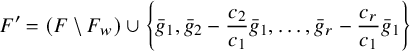 $$\begin{align*}F' = \left(F \setminus F_w\right) \cup \left\{\bar{g}_1, \bar{g}_2 - \frac{c_2}{c_1}\bar{g}_1,\ldots,\bar{g}_r - \frac{c_r}{c_1}\bar{g}_1 \right\} \end{align*}$$
be still a minimal generating set, and
 $\left | F^{\prime }_v \right | \in \{0,1\}$
for all
$\left | F^{\prime }_v \right | \in \{0,1\}$
for all
 $v \leq w$
. Iterate this process, letting
$v \leq w$
. Iterate this process, letting
 $F = F'$
. Eventually,
$F = F'$
. Eventually,
 $\left | F_v \right | \in \{0,1\}$
for all
$\left | F_v \right | \in \{0,1\}$
for all
 $v \in S_n$
. In particular, this F is upper triangular with respect to our total order (the minimal element in the support of each spline is unique to that spline), and so F generates a free
$v \in S_n$
. In particular, this F is upper triangular with respect to our total order (the minimal element in the support of each spline is unique to that spline), and so F generates a free
 $\mathbb {C}[t_\bullet ]$
-module.
$\mathbb {C}[t_\bullet ]$
-module.
We note that this submodule is precisely where this paper proves h-positivity in Theorem 9.2 and Corollary 9.3.
3.1 Implied conditions on splines
This subsection gives algebraic conditions that an element
 $\bar {\rho } \in \mathcal {M}_{\Gamma }$
must satisfy that are not explicitly in the definition. Specifically, given
$\bar {\rho } \in \mathcal {M}_{\Gamma }$
must satisfy that are not explicitly in the definition. Specifically, given
 $w,v \in S_n$
, we want to infer conditions on
$w,v \in S_n$
, we want to infer conditions on
 $\bar {\rho }(w) - \bar {\rho }(v)$
when
$\bar {\rho }(w) - \bar {\rho }(v)$
when
 $(w,v)$
is not necessarily an edge in
$(w,v)$
is not necessarily an edge in
 $\mathcal {G}_\Gamma $
. Let
$\mathcal {G}_\Gamma $
. Let
 $w,v \in S_n$
and
$w,v \in S_n$
and
 $(w=v_0,v_1,\ldots ,v_m=v)$
be a path from w to v in
$(w=v_0,v_1,\ldots ,v_m=v)$
be a path from w to v in
 $\mathcal {G}_\Gamma $
. Say for each edge
$\mathcal {G}_\Gamma $
. Say for each edge
 $(v_{k-1},v_k)$
that
$(v_{k-1},v_k)$
that
 $v_kv_{k-1}^{-1} = (i_k,j_k)$
, so that
$v_kv_{k-1}^{-1} = (i_k,j_k)$
, so that
 $\mathcal {L}(v_{k-1},v_k) = \left \langle t_{i_k} - t_{j_k}\right \rangle $
for each
$\mathcal {L}(v_{k-1},v_k) = \left \langle t_{i_k} - t_{j_k}\right \rangle $
for each
 $k=1,\ldots ,m$
. Then
$k=1,\ldots ,m$
. Then
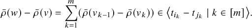 $$ \begin{align} \bar{\rho}(w)-\bar{\rho}(v) = \sum_{k=1}^{m} \left(\bar{\rho}(v_{k-1})-\bar{\rho}(v_k)\right) \in \left\langle t_{i_k} - t_{j_k} \mid k \in [m] \right\rangle. \end{align} $$
Define
 $$ \begin{align} I_B^w := \left\langle t_{w(i)}-t_{w(j)} \mid (i,j) \in B \subseteq E(T) \right\rangle. \end{align} $$
Lemma 3.3 below is particularly useful when
 $\bar {\rho } \in \mathcal {M}_{\Gamma }$
satisfies
$\bar {\rho } \in \mathcal {M}_{\Gamma }$
satisfies
 $\bar {\rho }(v) = 0$
for some
$\bar {\rho }(v) = 0$
for some
 $v \in S_n$
. Recall that we identify
$v \in S_n$
. Recall that we identify
 $B \subset E(\Gamma )$
with a subset of transpositions, and write
$B \subset E(\Gamma )$
with a subset of transpositions, and write
 $w\langle B \rangle $
for the left coset at w of the reflection subgroup generated by the transpositions in B.
$w\langle B \rangle $
for the left coset at w of the reflection subgroup generated by the transpositions in B.
Lemma 3.3. Let T be a spanning tree of
 $\Gamma $
. Let
$\Gamma $
. Let
 $v \in w\langle B \rangle $
, where
$v \in w\langle B \rangle $
, where
 $B \subseteq E(T)$
. If
$B \subseteq E(T)$
. If
 $\bar {\rho } \in \mathcal {M}_{\Gamma }$
, then
$\bar {\rho } \in \mathcal {M}_{\Gamma }$
, then
 $\bar {\rho }(w)-\bar {\rho }(v) \in I_B^w$
.
$\bar {\rho }(w)-\bar {\rho }(v) \in I_B^w$
.
Proof. Let
 $w^{-1}v = b_1\cdots b_m$
, where
$w^{-1}v = b_1\cdots b_m$
, where
 $b_1,\ldots ,b_m \in B$
. Let
$b_1,\ldots ,b_m \in B$
. Let
 $(w = v_0, v_1,\ldots , v_m=v)$
be the path from w to v, where
$(w = v_0, v_1,\ldots , v_m=v)$
be the path from w to v, where
 $v_{k}^{-1}v_{k-1} = b_k \in B$
for all
$v_{k}^{-1}v_{k-1} = b_k \in B$
for all
 $k \in [m]$
. Say that
$k \in [m]$
. Say that
 $v_{k}v_{k-1}^{-1} = (i_k,j_k)$
, so that
$v_{k}v_{k-1}^{-1} = (i_k,j_k)$
, so that
 $\mathcal {L}(v_{k-1},v_{k})= t_{i_k} - t_{j_k}$
. By Equation (3.1),
$\mathcal {L}(v_{k-1},v_{k})= t_{i_k} - t_{j_k}$
. By Equation (3.1),
 $$\begin{align*}\bar{\rho}(w)-\bar{\rho}(v) \in \left\langle t_{i_k} - t_{j_k} \mid k \in [m] \right\rangle. \end{align*}$$
For each
 $k \in [m]$
, since
$k \in [m]$
, since
 $v_kv_{k-1}^{-1}= (i_k,j_k)$
, we have that
$v_kv_{k-1}^{-1}= (i_k,j_k)$
, we have that
 $b_k = v_k^{-1}v_{k-1} = \left (v_k^{-1}(i_k),v_k^{-1}(j_k)\right )$
. Each edge
$b_k = v_k^{-1}v_{k-1} = \left (v_k^{-1}(i_k),v_k^{-1}(j_k)\right )$
. Each edge
 $b_k \in B$
, so the integers
$b_k \in B$
, so the integers
 $v_k^{-1}(i_k) = (wb_1\cdots b_k)^{-1}(i_k)$
and
$v_k^{-1}(i_k) = (wb_1\cdots b_k)^{-1}(i_k)$
and
 $v_{k}^{-1}(j_k) = (wb_1\cdots b_k)^{-1}(j_k)$
must be in the same connected component of
$v_{k}^{-1}(j_k) = (wb_1\cdots b_k)^{-1}(j_k)$
must be in the same connected component of
 $([n],B)$
.
$([n],B)$
.
Since
 $(wb_1\cdots b_k)^{-1} = (b_k\cdots b_1)w^{-1}$
, it follows that
$(wb_1\cdots b_k)^{-1} = (b_k\cdots b_1)w^{-1}$
, it follows that
 $w^{-1}(i_k)$
and
$w^{-1}(i_k)$
and
 $w^{-1}(j_k)$
are vertices in the same connected component of
$w^{-1}(j_k)$
are vertices in the same connected component of
 $([n],B)$
for all
$([n],B)$
for all
 $k \in [m]$
. If
$k \in [m]$
. If
 $(q_0,...,q_\ell )$
is a path in
$(q_0,...,q_\ell )$
is a path in
 $([n],B)$
from
$([n],B)$
from
 $q_0 = w^{-1}(i_k)$
to
$q_0 = w^{-1}(i_k)$
to
 $q_{\ell } = = w^{-1}(j_k)$
, then
$q_{\ell } = = w^{-1}(j_k)$
, then
 $t_{q_0} - t_{q_\ell } = \sum _{r=1}^\ell t_{q_{r-1}} - t_{q_r}$
, and thus,
$t_{q_0} - t_{q_\ell } = \sum _{r=1}^\ell t_{q_{r-1}} - t_{q_r}$
, and thus,
 $t_{w^{-1}(i_k)}-t_{w^{-1}(j_k)} \in I_B^e$
. It follows that
$t_{w^{-1}(i_k)}-t_{w^{-1}(j_k)} \in I_B^e$
. It follows that
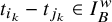 $t_{i_k} - t_{j_k} \in I_B^w$
for all
$t_{i_k} - t_{j_k} \in I_B^w$
for all
 $k \in [m]$
, and so
$k \in [m]$
, and so
 $\bar {\rho }(w)-\bar {\rho }(v)\in I_B^w$
.
$\bar {\rho }(w)-\bar {\rho }(v)\in I_B^w$
.
A monomial ideal in
 $\mathbb {C}[t_\bullet ]$
is an ideal I generated by monomials. Monomial ideals are particularly nice when computing intersections; if
$\mathbb {C}[t_\bullet ]$
is an ideal I generated by monomials. Monomial ideals are particularly nice when computing intersections; if
 $I_1 = \langle m_1,\ldots ,m_k\rangle $
and
$I_1 = \langle m_1,\ldots ,m_k\rangle $
and
 $I_2 = \langle n_1,\ldots ,n_\ell \rangle $
are both monomial ideals, then
$I_2 = \langle n_1,\ldots ,n_\ell \rangle $
are both monomial ideals, then
 $I_1 \cap I_2 = \langle \mathrm {lcm}(m_i,n_j) \mid i \in [k],\; j\in [\ell ]\rangle $
.
$I_1 \cap I_2 = \langle \mathrm {lcm}(m_i,n_j) \mid i \in [k],\; j\in [\ell ]\rangle $
.
Let T be a spanning tree of
 $\Gamma $
, where
$\Gamma $
, where
 $E(T) = \{(a_1,b_1),\ldots ,(a_{n-1},b_{n-1})\}$
. Ideals of the form
$E(T) = \{(a_1,b_1),\ldots ,(a_{n-1},b_{n-1})\}$
. Ideals of the form
 $\langle t_{a_i}-t_{b_i} \mid (a_i,b_i) \in B \subset E(T) \rangle $
can be considered monomial ideals, via the graded automorphism
$\langle t_{a_i}-t_{b_i} \mid (a_i,b_i) \in B \subset E(T) \rangle $
can be considered monomial ideals, via the graded automorphism
 $$\begin{align*}\mathbb{C}[t_1,\ldots,t_n] \cong \mathbb{C}[t_{a_1}-t_{b_1},\ldots,t_{a_{n-1}}-t_{b_{n-1}},t_n] \end{align*}$$
defined by
 $t_i \mapsto \begin {cases}t_{a_i}-t_{b_i} &\text {if } i \in [n-1] \\ t_n & \text {if }i=n \end {cases}$
. Since
$t_i \mapsto \begin {cases}t_{a_i}-t_{b_i} &\text {if } i \in [n-1] \\ t_n & \text {if }i=n \end {cases}$
. Since
 $t_i \mapsto t_{w(i)}$
is also a graded automorphism of
$t_i \mapsto t_{w(i)}$
is also a graded automorphism of
 $\mathbb {C}[t_\bullet ]$
, the ideals
$\mathbb {C}[t_\bullet ]$
, the ideals
 $I_B^w$
from Equation 3.2 can also be considered as monomial ideals (taking care to fix T and
$I_B^w$
from Equation 3.2 can also be considered as monomial ideals (taking care to fix T and
 $w \in S_n$
). We will fix T and w and then treat ideals of the form
$w \in S_n$
). We will fix T and w and then treat ideals of the form
 $I_B^w$
as monomial ideals to compute intersections in the proofs of Theorem 3.7 and Lemma 4.1 in the following two sections.
$I_B^w$
as monomial ideals to compute intersections in the proofs of Theorem 3.7 and Lemma 4.1 in the following two sections.
3.2 Coset splines and trees
This subsection establishes a set of splines called coset splines (Definition 3.4) that generate
 $\mathcal {M}_{\Gamma }$
as a module over the polynomial ring when
$\mathcal {M}_{\Gamma }$
as a module over the polynomial ring when
 $\Gamma $
is a tree. This subsection also identifies a subset of those coset splines that generate
$\Gamma $
is a tree. This subsection also identifies a subset of those coset splines that generate
 $\mathcal {M}_{\Gamma }$
as a ring when
$\mathcal {M}_{\Gamma }$
as a ring when
 $\Gamma $
is a tree.
$\Gamma $
is a tree.
Definition 3.4. Let
 $\Gamma $
be a tree,
$\Gamma $
be a tree, ![]() and
and
 $B \subseteq E$
. The coset spline at the identity
$B \subseteq E$
. The coset spline at the identity
 $\bar {f}_e^B \colon S_n \to \mathbb {C}[t_\bullet ]$
is
$\bar {f}_e^B \colon S_n \to \mathbb {C}[t_\bullet ]$
is
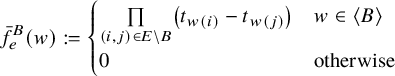 $$\begin{align*}\bar{f}_e^B(w) := \begin{cases} { \prod\limits_{(i,j) \in E \setminus B} \left(t_{w(i)} - t_{w(j)}\right)} & w \in \langle B \rangle \\ 0 & \text{otherwise} \end{cases} \end{align*}$$
The coset spline at w is
 $\bar {f_w^B} := w \cdot \bar {f}_e^B$
. We adopt the conventions that a product over the empty set
$\bar {f_w^B} := w \cdot \bar {f}_e^B$
. We adopt the conventions that a product over the empty set
 $\emptyset $
is
$\emptyset $
is
 $1$
(so
$1$
(so ![]() ) and that the subgroup generated by the empty set is the identity (so
) and that the subgroup generated by the empty set is the identity (so
 $\langle \emptyset \rangle = \{e\}$
).
$\langle \emptyset \rangle = \{e\}$
).
Example 3.5. Again, consider
 $\Gamma = \left ([3],\{(1,2),(2,3)\}\right )$
. Drawn below are three examples of coset splines on
$\Gamma = \left ([3],\{(1,2),(2,3)\}\right )$
. Drawn below are three examples of coset splines on
 $\mathcal {G}_\Gamma $
.
$\mathcal {G}_\Gamma $
.
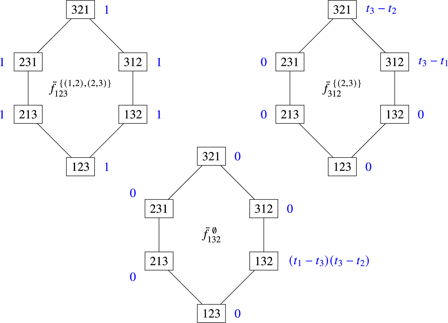
Lemma 3.6. When
 $\Gamma $
is a tree, coset splines are elements of
$\Gamma $
is a tree, coset splines are elements of
 $\mathcal {M}_{\Gamma }$
. Additionally, if
$\mathcal {M}_{\Gamma }$
. Additionally, if
 $w,v \in S_n$
are in the same coset of
$w,v \in S_n$
are in the same coset of
 $\langle B \rangle $
, then
$\langle B \rangle $
, then
 $\bar {f}_w^B = \bar {f}_v^B$
.
$\bar {f}_w^B = \bar {f}_v^B$
.
Proof. It suffices to show
 $\bar {f}_e^B$
is a spline. Let
$\bar {f}_e^B$
is a spline. Let
 $w \in \langle B \rangle $
and
$w \in \langle B \rangle $
and
 $v \in S_n$
, where
$v \in S_n$
, where
 $vw^{-1} = (i,j) \in E$
.
$vw^{-1} = (i,j) \in E$
.
If
 $(i,j) \in E \setminus B$
, then
$(i,j) \in E \setminus B$
, then
 $v \notin \langle B \rangle $
, and so
$v \notin \langle B \rangle $
, and so
 $\bar {f}_e^B(v) = 0$
. Thus,
$\bar {f}_e^B(v) = 0$
. Thus,
 $\bar {f}_e^B(w) - \bar {f}_w^B(v) = t_{w(i)}-t_{w(j)} \in \mathcal {L}(w,v)$
, as desired.
$\bar {f}_e^B(w) - \bar {f}_w^B(v) = t_{w(i)}-t_{w(j)} \in \mathcal {L}(w,v)$
, as desired.
If
 $(i,j) \in B$
, then
$(i,j) \in B$
, then
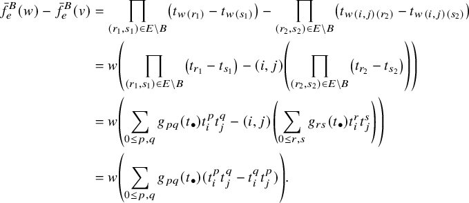 $$ \begin{align*} \bar{f}_e^B(w) - \bar{f}_e^B(v) &= \prod_{(r_1,s_1) \in E \setminus B} \left(t_{w(r_1)} - t_{w(s_1)}\right) - \prod_{(r_2,s_2) \in E \setminus B} \left(t_{w(i,j)(r_2)} - t_{w(i,j)(s_2)}\right) \\ &= w\left(\prod_{(r_1,s_1) \in E \setminus B} \left(t_{r_1} - t_{s_1}\right) - (i,j)\left(\prod_{(r_2,s_2) \in E \setminus B} \left(t_{r_2} - t_{s_2}\right)\right)\right)\\ &= w\left(\sum_{0\leq p,q} g_{pq}(t_\bullet) t_i^p t_j^q -(i,j)\left(\sum_{0\leq r,s} g_{rs}(t_\bullet) t_i^r t_j^s\right)\right)\\ &= w\left(\sum_{0\leq p,q} g_{pq}(t_\bullet) (t_i^p t_j^q- t_i^q t_j^p)\right). \end{align*} $$
As
 $t_i^p t_j^q- t_i^q t_j^p \in \left \langle t_i-t_j\right \rangle $
, it follows that
$t_i^p t_j^q- t_i^q t_j^p \in \left \langle t_i-t_j\right \rangle $
, it follows that
 $\bar {f}_e^B(w) - \bar {f}_e^B(v) \in \left \langle t_{w(i)} - t_{w(j)} \right \rangle = \mathcal {L}(w,v)$
. Thus,
$\bar {f}_e^B(w) - \bar {f}_e^B(v) \in \left \langle t_{w(i)} - t_{w(j)} \right \rangle = \mathcal {L}(w,v)$
. Thus,
 $\bar {f}_e^B$
is a spline.
$\bar {f}_e^B$
is a spline.
Now we prove that coset splines are uniquely determined by the coset. For all
 $u \in \langle B \rangle $
, we have
$u \in \langle B \rangle $
, we have
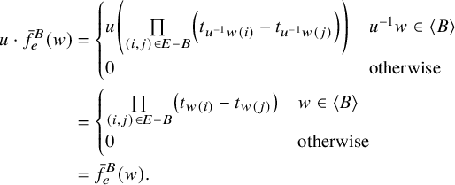 $$ \begin{align*} u \cdot \bar{f}_e^B(w) &= \begin{cases}{ u\left(\prod\limits_{(i,j) \in E - B} \left(t_{u^{-1}w(i)} - t_{u^{-1}w(j)}\right)\right)} & u^{-1}w \in \langle B \rangle \\ 0 & \text{otherwise} \end{cases}\\ &= \begin{cases} { \prod\limits_{(i,j) \in E - B} \left(t_{w(i)} - t_{w(j)}\right)} & w \in \langle B \rangle \\ 0 & \text{otherwise} \\ \end{cases}\\ &= \bar{f}_e^B(w). \end{align*} $$
If
 $w\langle B \rangle = v\langle B \rangle $
, then
$w\langle B \rangle = v\langle B \rangle $
, then
 $w=vu$
, for some
$w=vu$
, for some
 $u \in \langle B \rangle $
, and so
$u \in \langle B \rangle $
, and so
 $$\begin{align*}\bar{f}_w^B = w\cdot \bar{f}_e^B = (vu)\cdot \bar{f}_e^B = v\cdot (u\cdot \bar{f}_e^B) = v\cdot \bar{f}_e^B = \bar{f}_v^B.\\[-34pt] \end{align*}$$
Note that the following Theorem 3.7 is independent of the left or right module structure.
Theorem 3.7. Let
 $\Gamma $
be a tree. The set of coset splines
$\Gamma $
be a tree. The set of coset splines
 $\{\bar {f}_w^B \mid w \in S_n,\; B \subseteq E(\Gamma )\}$
is a
$\{\bar {f}_w^B \mid w \in S_n,\; B \subseteq E(\Gamma )\}$
is a
 $\mathbb {C}[t_\bullet ]$
-generating set of
$\mathbb {C}[t_\bullet ]$
-generating set of
 $\mathcal {M}_{\Gamma }$
.
$\mathcal {M}_{\Gamma }$
.
Proof. Let
 $\bar {\rho }\in \mathcal {M}_{\Gamma }$
, we will show that
$\bar {\rho }\in \mathcal {M}_{\Gamma }$
, we will show that
 $\bar {\rho } \in \mathbb {C}[t_\bullet ]\{\bar {f}_B^w \mid w \in S_n, B \subseteq E(\Gamma )\}$
by induction on containment of the support
$\bar {\rho } \in \mathbb {C}[t_\bullet ]\{\bar {f}_B^w \mid w \in S_n, B \subseteq E(\Gamma )\}$
by induction on containment of the support
 $\mathrm {supp}(\bar {\rho })$
. If
$\mathrm {supp}(\bar {\rho })$
. If
 $\bar {\rho } \equiv 0$
, this is clearly in the span of the coset splines, and the base case
$\bar {\rho } \equiv 0$
, this is clearly in the span of the coset splines, and the base case
 $\mathrm {supp}(\bar {\rho }) = \emptyset $
is done. Otherwise,
$\mathrm {supp}(\bar {\rho }) = \emptyset $
is done. Otherwise,
 $\mathrm {supp}(\bar {\rho }) \neq \emptyset $
, and we assume all splines
$\mathrm {supp}(\bar {\rho }) \neq \emptyset $
, and we assume all splines
 $\bar {\kappa }$
where
$\bar {\kappa }$
where
 $\mathrm {supp}(\bar {\kappa }) \subsetneq \mathrm {supp}(\bar {\rho })$
are in
$\mathrm {supp}(\bar {\kappa }) \subsetneq \mathrm {supp}(\bar {\rho })$
are in
 $\mathbb {C}[t_\bullet ]\{\bar {f}_B^w \mid w \in S_n, B \subseteq E(\Gamma )\}$
. Replacing
$\mathbb {C}[t_\bullet ]\{\bar {f}_B^w \mid w \in S_n, B \subseteq E(\Gamma )\}$
. Replacing
 $\bar {\rho }$
by
$\bar {\rho }$
by ![]() if necessary, we assume
if necessary, we assume
 $\bar {\rho }(e) = 0$
. This also handles the case where
$\bar {\rho }(e) = 0$
. This also handles the case where
 $\mathrm {supp}(\bar {\rho }) = S_n$
.
$\mathrm {supp}(\bar {\rho }) = S_n$
.
Fix
 $w \in S_n$
such that
$w \in S_n$
such that
 $\bar {\rho }(w) \neq 0$
and w is adjacent in
$\bar {\rho }(w) \neq 0$
and w is adjacent in
 $\mathcal {G}_\Gamma $
to some
$\mathcal {G}_\Gamma $
to some
 $w' \in S_n$
where
$w' \in S_n$
where
 $\bar {\rho }(w') = 0$
. Define
$\bar {\rho }(w') = 0$
. Define
Since
 $\bar {\rho }(w') = 0$
, this set is nonempty. Each element in
$\bar {\rho }(w') = 0$
, this set is nonempty. Each element in
 $\mathcal {B}_w$
is a generating set for a reflection subgroup whose left coset at w contains an element not in
$\mathcal {B}_w$
is a generating set for a reflection subgroup whose left coset at w contains an element not in
 $\mathrm {supp}(\bar {\rho })$
. Note if
$\mathrm {supp}(\bar {\rho })$
. Note if
 $B \subset B'$
and
$B \subset B'$
and
 $B \in \mathcal {B}_w$
, then
$B \in \mathcal {B}_w$
, then
 $B' \in \mathcal {B}_w$
.
$B' \in \mathcal {B}_w$
.
By Lemma 3.3,
Following the logic of Subsection 3.1 (i.e., treating
 $\{t_{w(i)} - t_{w(j)} \mid (i,j) \in E(\Gamma )\}$
as variables),
$\{t_{w(i)} - t_{w(j)} \mid (i,j) \in E(\Gamma )\}$
as variables),
 $\mathcal {I}_\rho ^w$
is a monomial ideal generated by the monomials that are contained within every element of the intersection.
$\mathcal {I}_\rho ^w$
is a monomial ideal generated by the monomials that are contained within every element of the intersection.
A monomial
 $\mathfrak {m} = { \prod\limits _{(i,j) \in E} \left (t_{w(i)}-t_{w(j)}\right )^{\alpha _{ij}}}$
is contained within the ideal
$\mathfrak {m} = { \prod\limits _{(i,j) \in E} \left (t_{w(i)}-t_{w(j)}\right )^{\alpha _{ij}}}$
is contained within the ideal
 $\mathcal {I}_\rho ^w$
if and only if for every
$\mathcal {I}_\rho ^w$
if and only if for every
 $B \in \mathcal {B}_w$
, there is at least one
$B \in \mathcal {B}_w$
, there is at least one
 $(i,j) \in B$
such that
$(i,j) \in B$
such that
 $\alpha _{ij}> 0$
. For generators of
$\alpha _{ij}> 0$
. For generators of
 $\mathcal {I}_\rho ^w$
, it suffices to consider only those monomials such that
$\mathcal {I}_\rho ^w$
, it suffices to consider only those monomials such that
 $\alpha _{ij} \in \{0,1\}$
for all
$\alpha _{ij} \in \{0,1\}$
for all
 $(i,j) \in E(\Gamma )$
. Since
$(i,j) \in E(\Gamma )$
. Since
 $\alpha _{ij} \in \{0,1\}$
, the monomials that generate
$\alpha _{ij} \in \{0,1\}$
, the monomials that generate
 $\mathcal {I}_\rho ^w$
are a subset of
$\mathcal {I}_\rho ^w$
are a subset of
 $\{\bar {f}_w^B(w) \mid B \subseteq E(\Gamma )\}$
. In particular, we have the equality
$\{\bar {f}_w^B(w) \mid B \subseteq E(\Gamma )\}$
. In particular, we have the equality
 $\left \langle \bar {f}_w^D(w) \mid D \subseteq E(\Gamma ),\;\bar {f}_w^D(w) \in \mathcal {I}_\rho ^w \right \rangle = \mathcal {I}_\rho ^w$
.
$\left \langle \bar {f}_w^D(w) \mid D \subseteq E(\Gamma ),\;\bar {f}_w^D(w) \in \mathcal {I}_\rho ^w \right \rangle = \mathcal {I}_\rho ^w$
.
Consider the coset splines
 $\{\bar {f}_w^D \mid \bar {f}_w^D(w) \in \mathcal {I}_\rho ^w\}$
. By definition, for any
$\{\bar {f}_w^D \mid \bar {f}_w^D(w) \in \mathcal {I}_\rho ^w\}$
. By definition, for any
 $D \subset E(\Gamma )$
,
$D \subset E(\Gamma )$
,
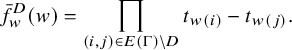 $$\begin{align*}\bar{f}_w^{D}(w) = \prod_{(i,j) \in E(\Gamma)\setminus D} t_{w(i)} - t_{w(j)}. \end{align*}$$
Now
 $\bar {f}_w^{D}(w)\in \mathcal {I}_\rho ^w$
if and only if
$\bar {f}_w^{D}(w)\in \mathcal {I}_\rho ^w$
if and only if
 $\left (E(\Gamma )\setminus D\right ) \cap B \neq \emptyset $
for all
$\left (E(\Gamma )\setminus D\right ) \cap B \neq \emptyset $
for all
 $B \in \mathcal {B}_w$
. Thus,
$B \in \mathcal {B}_w$
. Thus,
 $\bar {f}_w^{D}(w)\in \mathcal {I}_\rho ^w$
if and only if
$\bar {f}_w^{D}(w)\in \mathcal {I}_\rho ^w$
if and only if
 $B \not \subset D$
for all
$B \not \subset D$
for all
 $B \in \mathcal {B}_w$
. Since
$B \in \mathcal {B}_w$
. Since
 $\mathcal {B}_w$
is closed under supersets,
$\mathcal {B}_w$
is closed under supersets,
 $\bar {f}_w^{D}(w)\in \mathcal {I}_\rho ^w$
if and only if
$\bar {f}_w^{D}(w)\in \mathcal {I}_\rho ^w$
if and only if
 $D \notin \mathcal {B}_w$
. Thus,
$D \notin \mathcal {B}_w$
. Thus,
 $$ \begin{align*} \bar{\rho}(w) \in \mathcal{I}_\rho^w = \left\langle \bar{f}_w^D(w) \mid \text{ for all } v \in w\langle D \rangle, \; \bar{\rho}(v) \neq 0 \right\rangle. \end{align*} $$
Let
 $\bar {f} \in \mathbb {C}[t_\bullet ]\{\bar {f}_w^D \mid \text { for all } v \in w\langle D \rangle ,\; \bar {\rho }(v) \neq 0 \}$
such that
$\bar {f} \in \mathbb {C}[t_\bullet ]\{\bar {f}_w^D \mid \text { for all } v \in w\langle D \rangle ,\; \bar {\rho }(v) \neq 0 \}$
such that
 $\bar {\rho }(w) = \bar {f}(w)$
(a different
$\bar {\rho }(w) = \bar {f}(w)$
(a different
 $\bar {f}$
may be chosen for the left and right module structure, but either way, such a
$\bar {f}$
may be chosen for the left and right module structure, but either way, such a
 $\bar {f}$
exists since it is only required to agree with
$\bar {f}$
exists since it is only required to agree with
 $\bar {\rho }$
at w). Since
$\bar {\rho }$
at w). Since
 $\mathrm {supp}(\bar {f}) \subseteq \mathrm {supp}(\bar {\rho })$
and
$\mathrm {supp}(\bar {f}) \subseteq \mathrm {supp}(\bar {\rho })$
and
 $\bar {f}(w) = \bar {\rho }(w) \neq 0$
, it follows that
$\bar {f}(w) = \bar {\rho }(w) \neq 0$
, it follows that
 $\mathrm {supp}(\bar {\rho }) \supsetneq \mathrm {supp}(\bar {\rho }-\bar {f})$
. Thus,
$\mathrm {supp}(\bar {\rho }) \supsetneq \mathrm {supp}(\bar {\rho }-\bar {f})$
. Thus,
 $\bar {\rho }-\bar {f} \in \mathbb {C}[t_\bullet ]\{\bar {f}_B^w \mid w \in S_n, B \subseteq E(\Gamma )\}$
. Since
$\bar {\rho }-\bar {f} \in \mathbb {C}[t_\bullet ]\{\bar {f}_B^w \mid w \in S_n, B \subseteq E(\Gamma )\}$
. Since
 $\bar {f}$
is also a sum of coset splines,
$\bar {f}$
is also a sum of coset splines,
 $\bar {\rho } \in \mathbb {C}[t_\bullet ]\{\bar {f}_B^w \mid w \in S_n, B \subseteq E(\Gamma )\}$
.
$\bar {\rho } \in \mathbb {C}[t_\bullet ]\{\bar {f}_B^w \mid w \in S_n, B \subseteq E(\Gamma )\}$
.
The collection of all coset splines is not a minimal generating set. One might significantly decrease the size of this set by fixing the linear order on
 $S_n$
in the proof of Lemma 3.2, and only considering the largest (by support) coset splines supported ‘above’ a permutation. There is no guarantee that these generators are minimal for all degrees, but it is easy to reason that this collection is minimal for the module
$S_n$
in the proof of Lemma 3.2, and only considering the largest (by support) coset splines supported ‘above’ a permutation. There is no guarantee that these generators are minimal for all degrees, but it is easy to reason that this collection is minimal for the module
 $\mathcal {M}_{\Gamma }^{\leq 2}$
generated by the constant, linear and quadratic splines.
$\mathcal {M}_{\Gamma }^{\leq 2}$
generated by the constant, linear and quadratic splines.
We also achieve a generating set for
 $\mathcal {M}_{\Gamma }$
as a ring in Corollary 3.8 below.
$\mathcal {M}_{\Gamma }$
as a ring in Corollary 3.8 below.
Corollary 3.8. Let
 $\Gamma $
be a tree. The constant and linear coset splines along with either
$\Gamma $
be a tree. The constant and linear coset splines along with either
 $\{\bar {t}_i \mid i \in [n]\}$
or
$\{\bar {t}_i \mid i \in [n]\}$
or
 $\{\bar {x}_i \mid i \in [n]\}$
generate
$\{\bar {x}_i \mid i \in [n]\}$
generate
 $\mathcal {M}_{\Gamma }$
as a ring.
$\mathcal {M}_{\Gamma }$
as a ring.
Proof. It follows immediately from the definition that
 $$\begin{align*}f_w^B = \prod_{s \in E(\Gamma) \setminus B}f_w^{E(\Gamma) \setminus\{s\}}. \end{align*}$$
So every coset spline except ![]() is a product of linear coset splines, which generate
is a product of linear coset splines, which generate
 $\mathcal {M}_{\Gamma }$
together with either
$\mathcal {M}_{\Gamma }$
together with either
 $\{\bar {t}_i \mid i \in [n]\}$
or
$\{\bar {t}_i \mid i \in [n]\}$
or
 $\{\bar {x}_i \mid i \in [n]\}$
by Theorem 3.7.
$\{\bar {x}_i \mid i \in [n]\}$
by Theorem 3.7.
We can leverage Theorem 3.7 to compute
 $\mathcal {M}_{\Gamma }$
for all graphs
$\mathcal {M}_{\Gamma }$
for all graphs
 $\Gamma $
. Any graph
$\Gamma $
. Any graph
 $\Gamma $
can be expressed as the union of spanning trees
$\Gamma $
can be expressed as the union of spanning trees
 $\Gamma = T_1 \cup \cdots \cup T_k$
. Lemma 2.16 says that
$\Gamma = T_1 \cup \cdots \cup T_k$
. Lemma 2.16 says that
 ${ \mathcal {M}_{\Gamma } = \bigcap _{i=1}^k \mathcal {M}_{T_i}}$
, and Theorem 3.7 gives explicit generators for each
${ \mathcal {M}_{\Gamma } = \bigcap _{i=1}^k \mathcal {M}_{T_i}}$
, and Theorem 3.7 gives explicit generators for each
 $\mathcal {M}_{T_i}$
. This is most useful in computer calculations, where the task of constructing modules from generators and intersecting them can be completed by a computer algebra system.
$\mathcal {M}_{T_i}$
. This is most useful in computer calculations, where the task of constructing modules from generators and intersecting them can be completed by a computer algebra system.
4 Connectedness and
$\mathcal {M}_{\Gamma }^k$

This section proves an equivalence between the k-connectivity of
 $\Gamma $
and which graded pieces of the representation
$\Gamma $
and which graded pieces of the representation
 $\mathbf {ch}\left (\mathrm {L}_{\Gamma }\right )$
are trivial.
$\mathbf {ch}\left (\mathrm {L}_{\Gamma }\right )$
are trivial.
Lemma 4.1 below infers new conditions on
 $\mathcal {M}_{\Gamma }$
from collections of vertex-disjoint paths in
$\mathcal {M}_{\Gamma }$
from collections of vertex-disjoint paths in
 $\Gamma $
.
$\Gamma $
.
Lemma 4.1. Say that there exist k vertex-disjoint paths from i to j in
 $\Gamma $
. Let
$\Gamma $
. Let
 $\Gamma ' = ([n],E(\Gamma ) \cup \{(i,j)\})$
. Then
$\Gamma ' = ([n],E(\Gamma ) \cup \{(i,j)\})$
. Then
 $\mathcal {M}_{\Gamma }^{k-1} = \mathcal {M}_{\Gamma '}^{k-1}$
.
$\mathcal {M}_{\Gamma }^{k-1} = \mathcal {M}_{\Gamma '}^{k-1}$
.
Proof. We will show both directions of containment. Clearly,
 $\mathcal {M}_{\Gamma }^{k-1} \supseteq \mathcal {M}_{\Gamma '}^{k-1}$
.
$\mathcal {M}_{\Gamma }^{k-1} \supseteq \mathcal {M}_{\Gamma '}^{k-1}$
.
Say that
 $\bar {\rho } \in \mathcal {M}_{\Gamma }^{k-1}$
, and let
$\bar {\rho } \in \mathcal {M}_{\Gamma }^{k-1}$
, and let
 $w,v \in S_n$
such that
$w,v \in S_n$
such that
 $w^{-1}v = (i,j)$
. Let
$w^{-1}v = (i,j)$
. Let
 $p_r = (i,s_{r,1},\ldots ,s_{r,\ell _r},j)$
for
$p_r = (i,s_{r,1},\ldots ,s_{r,\ell _r},j)$
for
 $r=1,\ldots ,k$
be the k vertex-disjoint paths from i to j in
$r=1,\ldots ,k$
be the k vertex-disjoint paths from i to j in
 $\Gamma $
. By Lemma 3.3,
$\Gamma $
. By Lemma 3.3,
 $$ \begin{align*} \bar{\rho}(w)- \bar{\rho}(v)&\in \left\langle t_{w(i)}-t_{w(s_{r,1})},t_{w(s_{r,1})}-t_{w(s_{r,2})},\ldots,t_{w(s_{r,\ell_r})}-t_{w(j)}\right\rangle \\ &= \left\langle t_{w(i)}-t_{w(j)}, t_{w(i)}-t_{w(s_{r,1})},\ldots,t_{w(s_{r,\ell_r-1})}-t_{w(s_{r,\ell_r})}\right\rangle \end{align*} $$
for all
 $r=1,\ldots ,k$
. Since the paths
$r=1,\ldots ,k$
. Since the paths
 $p_1,\ldots ,p_k$
are vertex independent, the set of edges
$p_1,\ldots ,p_k$
are vertex independent, the set of edges
 $$\begin{align*}A=\{(i,j)\} \cup \bigcup_{r=1}^k \{(i,s_{r,1}),(s_{r,1},s_{r,2}),\ldots,(s_{r,\ell_r-1},s_{r,\ell_r})\} \end{align*}$$
contains no cycles and thus forms a tree. In particular, we may consider
 $\{t_{a}-t_{b} \mid (a,b) \in A\}$
as monomials in
$\{t_{a}-t_{b} \mid (a,b) \in A\}$
as monomials in
 $\mathbb {C}[t_\bullet ]$
. Let
$\mathbb {C}[t_\bullet ]$
. Let
 $s_{r,0} := i$
when it is convenient for indexing. It remains to compute
$s_{r,0} := i$
when it is convenient for indexing. It remains to compute
 $$ \begin{align*} \bar{\rho}(w) &\in \bigcap_{r=1}^k \left\langle t_{w(i)}-t_{w(j)}, t_{w(s_{r,0})}-t_{w(s_{r,1})},\ldots,t_{w(s_{r,\ell_r-1})}-t_{w(s_{r,\ell_r})}\right\rangle \\ &= \left\langle t_{w(i)}-t_{w(j)},\left. \prod_{r=1}^k t_{w(s_{r,m_r-1})}-t_{w(s_{r,m_r})}\right| 0 < m_r \leq \ell_r \right\rangle. \end{align*} $$
Each generator of this ideal is a homogeneous polynomial, one of degree
 $1$
and all others of degree k. Since
$1$
and all others of degree k. Since
 $\bar {\rho }(w)-\bar {\rho }(v)$
is degree
$\bar {\rho }(w)-\bar {\rho }(v)$
is degree
 $k-1$
, it follows that
$k-1$
, it follows that
 $\bar {\rho }(w)-\bar {\rho }(v) \in \langle t_{w(i)} - t_{w(j)}\rangle $
.
$\bar {\rho }(w)-\bar {\rho }(v) \in \langle t_{w(i)} - t_{w(j)}\rangle $
.
Since
 $v,w$
were arbitrary such that
$v,w$
were arbitrary such that
 $w^{-1}v = (i,j)$
, we know that
$w^{-1}v = (i,j)$
, we know that
 $\bar {\rho } \in \mathcal {M}_{\Gamma '}^{k-1}$
. Since
$\bar {\rho } \in \mathcal {M}_{\Gamma '}^{k-1}$
. Since
 $\bar {\rho }$
was arbitrary,
$\bar {\rho }$
was arbitrary,
 $\mathcal {M}_{\Gamma }^{k-1} \subseteq \mathcal {M}_{\Gamma '}^{k-1}$
.
$\mathcal {M}_{\Gamma }^{k-1} \subseteq \mathcal {M}_{\Gamma '}^{k-1}$
.
Theorem 4.2. Let
 $\Gamma = ([n],E)$
be a connected graph on n vertices. The following are equivalent:
$\Gamma = ([n],E)$
be a connected graph on n vertices. The following are equivalent:
-
1.
$\Gamma $
is k-connected. -
2.
$\mathcal {M}_{\Gamma }^d = \mathcal {M}_{K_n}^d$
for all
$d<k$
, where
$K_n$
is the complete graph. -
3.
$\mathbf {ch}\left (\mathrm {L}_{\Gamma }\right )_{d}$
is trivial for all
$d<k$
.


Proof. (1)
 $\Rightarrow $
(2). If
$\Rightarrow $
(2). If
 $\Gamma $
is k-connected, by Menger’s theorem, every
$\Gamma $
is k-connected, by Menger’s theorem, every
 $(i,j) \in [n]\times [n]$
has k vertex-disjoint paths connecting them in
$(i,j) \in [n]\times [n]$
has k vertex-disjoint paths connecting them in
 $\Gamma $
. By Lemma 4.1,
$\Gamma $
. By Lemma 4.1,
 $\mathcal {M}_{\Gamma }^{k-1} = \mathcal {M}_{K_n}^{k-1}$
.
$\mathcal {M}_{\Gamma }^{k-1} = \mathcal {M}_{K_n}^{k-1}$
.
(2)
 $\Rightarrow $
(3). The ring
$\Rightarrow $
(3). The ring
 $\mathcal {M}_{K_n}$
corresponds to the equivariant cohomology of the full flag variety, where the dot action is known to be trivial [Reference Tymoczko28].
$\mathcal {M}_{K_n}$
corresponds to the equivariant cohomology of the full flag variety, where the dot action is known to be trivial [Reference Tymoczko28].
(3)
 $\Rightarrow $
(1). Assume that
$\Rightarrow $
(1). Assume that
 $\Gamma $
is not k-connected. Let d be the integer such that
$\Gamma $
is not k-connected. Let d be the integer such that
 $\Gamma $
is d-connected but not
$\Gamma $
is d-connected but not
 $(d+1)$
-connected (so
$(d+1)$
-connected (so
 $0 < d < k$
). We will show that
$0 < d < k$
). We will show that
 $\mathbf {ch}\left (\mathrm {L}_{\Gamma }\right )_d$
is not trivial. Then
$\mathbf {ch}\left (\mathrm {L}_{\Gamma }\right )_d$
is not trivial. Then
 $\Gamma $
has a cut set of size d, and so
$\Gamma $
has a cut set of size d, and so
 $\Gamma $
is (isomorphic to) a sub-graph of the graph
$\Gamma $
is (isomorphic to) a sub-graph of the graph
 $H = ([n],\{(i,j) \mid 1 \leq i<j<\ell +d\text { or } \ell < i < j \leq n\})$
drawn below:
$H = ([n],\{(i,j) \mid 1 \leq i<j<\ell +d\text { or } \ell < i < j \leq n\})$
drawn below:
(the center
 $K_{d}$
is the cut set). The graph H is also d-connected. By (1)
$K_{d}$
is the cut set). The graph H is also d-connected. By (1)
 $\Rightarrow $
(2), the graded pieces
$\Rightarrow $
(2), the graded pieces
 $\mathcal {M}_{\Gamma }^p = \mathcal {M}_{H}^p = \mathcal {M}_{K_n}^p$
for all
$\mathcal {M}_{\Gamma }^p = \mathcal {M}_{H}^p = \mathcal {M}_{K_n}^p$
for all
 $0 \leq p < d$
. Since
$0 \leq p < d$
. Since
 $\Gamma $
is an edge-subgraph of H, it follows directly from the definitions that
$\Gamma $
is an edge-subgraph of H, it follows directly from the definitions that
 $\mathcal {M}_{\Gamma } \supseteq \mathcal {M}_{H}$
.
$\mathcal {M}_{\Gamma } \supseteq \mathcal {M}_{H}$
.
If
 $I = \left \langle t_1,...,t_n \right \rangle $
, then for any graded
$I = \left \langle t_1,...,t_n \right \rangle $
, then for any graded
 $\mathbb {C}[t_\bullet ]$
-module
$\mathbb {C}[t_\bullet ]$
-module ![]() , the following equality is by definition
, the following equality is by definition
Since multiplication by elements in I must increase degree, the d-th degree component of
 $I\mathcal {M}_{\Gamma }$
and the d-th degree component of
$I\mathcal {M}_{\Gamma }$
and the d-th degree component of
 $I\mathcal {M}_{H}$
are equal. In particular,
$I\mathcal {M}_{H}$
are equal. In particular,
 $$\begin{align*}I\mathcal{M}_{\Gamma} \cap \mathcal{M}_{\Gamma}^d = I\left(\mathcal{M}_{\Gamma}^{\leq d-1}\right) \cap \mathcal{M}_{\Gamma}^d = I\left(\mathcal{M}_{H}^{\leq d-1}\right) \cap \mathcal{M}_{\Gamma}^d = I\mathcal{M}_{H} \cap \mathcal{M}_{\Gamma}^d. \end{align*}$$
It follows that for the quotients
we get containment in the vector spaces
In particular, the representation with character
 $\mathbf {ch}\left (\mathrm {L}_{H}\right )_d$
is a sub-representation of the representation with character
$\mathbf {ch}\left (\mathrm {L}_{H}\right )_d$
is a sub-representation of the representation with character
 $\mathbf {ch}\left (\mathrm {L}_{\Gamma }\right )_d$
. The graph H is in fact a Hessenberg graph, and it is easy to compute with P-tableaux from [Reference Shareshian and Wachs25] that the d-th graded piece of
$\mathbf {ch}\left (\mathrm {L}_{\Gamma }\right )_d$
. The graph H is in fact a Hessenberg graph, and it is easy to compute with P-tableaux from [Reference Shareshian and Wachs25] that the d-th graded piece of
 $\mathbf {ch}\left (\mathrm {L}_{H}\right )$
is non-trivial, so the d-th graded piece of
$\mathbf {ch}\left (\mathrm {L}_{H}\right )$
is non-trivial, so the d-th graded piece of
 $\mathbf {ch}\left (\mathrm {L}_{\Gamma }\right )$
contains a nontrivial sub-representation and is thus nontrivial.
$\mathbf {ch}\left (\mathrm {L}_{\Gamma }\right )$
contains a nontrivial sub-representation and is thus nontrivial.
Remark 4.3. The graph H in the proof of Theorem 4.2 is the Hessenberg graph associated to the vector
 $$\begin{align*}h = (\overbrace{\ell+d,\ldots,\ell+d}^{\ell \text{ times}},n,\ldots,n). \end{align*}$$
The
 $3+1$
– and
$3+1$
– and
 $2+2$
–free poset P on
$2+2$
–free poset P on
 $[n]$
for which H is the indifference graph has relations
$[n]$
for which H is the indifference graph has relations
 $\{i <_P j \mid i \in [\ell ],\; j \in \{d+\ell +1,\ldots ,n\}\}$
.
$\{i <_P j \mid i \in [\ell ],\; j \in \{d+\ell +1,\ldots ,n\}\}$
.
The following corollary is a consequence of Theorem 4.2.
Corollary 4.4. If
 $\Gamma $
is k-connected, then
$\Gamma $
is k-connected, then
 $\mathbf {ch}\left (\mathrm {R}_{\Gamma }\right )_d$
is equal to
$\mathbf {ch}\left (\mathrm {R}_{\Gamma }\right )_d$
is equal to
 $\mathbf {ch}\left (\mathrm {R}_{K_n}\right )_d$
, which is the d-th degree piece of the graded regular representation.
$\mathbf {ch}\left (\mathrm {R}_{K_n}\right )_d$
, which is the d-th degree piece of the graded regular representation.
5 Generators for linear splines
The remaining sections are devoted to computing the first degree piece of the graded symmetric functions
 $\mathbf {ch}\left (\mathrm {L}_{\Gamma }\right )$
and
$\mathbf {ch}\left (\mathrm {L}_{\Gamma }\right )$
and
 $\mathbf {ch}\left (\mathrm {R}_{\Gamma }\right )$
for all connected graphs
$\mathbf {ch}\left (\mathrm {R}_{\Gamma }\right )$
for all connected graphs
 $\Gamma $
. We show that the first degree piece of
$\Gamma $
. We show that the first degree piece of
 $\mathcal {M}_{\Gamma }$
is computable from the data of cut vertices and cut edges, in particular the block-cut tree of
$\mathcal {M}_{\Gamma }$
is computable from the data of cut vertices and cut edges, in particular the block-cut tree of
 $\Gamma $
(Definition 6.2).
$\Gamma $
(Definition 6.2).
This section defines a set
 $\mathcal {F}_\Gamma $
that we will eventually show is a
$\mathcal {F}_\Gamma $
that we will eventually show is a
 $\mathbb {C}$
-spanning set for
$\mathbb {C}$
-spanning set for
 $\mathcal {M}_{\Gamma }^1$
. Subsection 5.1 proves several
$\mathcal {M}_{\Gamma }^1$
. Subsection 5.1 proves several
 $\mathbb {C}$
-linear relations within the set
$\mathbb {C}$
-linear relations within the set
 $\mathcal {F}_\Gamma $
that will turn out to be sufficient for reducing to a basis.
$\mathcal {F}_\Gamma $
that will turn out to be sufficient for reducing to a basis.
First, we will introduce (in fact, reintroduce) a collection of linear splines that depend on cut edges in
 $\Gamma $
. Let
$\Gamma $
. Let
 $s = (i,j)$
be a cut edge of
$s = (i,j)$
be a cut edge of
 $\Gamma $
, and let
$\Gamma $
, and let
 $G_s$
be one of the two connected components of
$G_s$
be one of the two connected components of
 $([n],E(\Gamma ) \setminus \{s\})$
. We are free to choose either component; see Remark 5.1 below. For each subset
$([n],E(\Gamma ) \setminus \{s\})$
. We are free to choose either component; see Remark 5.1 below. For each subset
 $A \subset [n]$
such that
$A \subset [n]$
such that
 $\left | A \right | = \left | G_s \right |$
, we define
$\left | A \right | = \left | G_s \right |$
, we define
 $\bar {f}_A^s \colon S_n \to \mathbb {C}[t_\bullet ]$
by
$\bar {f}_A^s \colon S_n \to \mathbb {C}[t_\bullet ]$
by
for all
 $w \in S_n$
. We associate to
$w \in S_n$
. We associate to
 $\Gamma $
the collection
$\Gamma $
the collection
Note that these splines
 $\bar {f}_A^s$
are actually the linear coset splines from Definition 3.4. We make the change in notation for several reasons, one being that the subset A uniquely determines the coset whose support is
$\bar {f}_A^s$
are actually the linear coset splines from Definition 3.4. We make the change in notation for several reasons, one being that the subset A uniquely determines the coset whose support is
 $\bar {f}_A^s$
(as opposed to many elements w defining the same
$\bar {f}_A^s$
(as opposed to many elements w defining the same
 $\bar {f}_w^B$
). Since
$\bar {f}_w^B$
). Since
 $G_s$
is one of two connected components in the graph
$G_s$
is one of two connected components in the graph
 $([n],E(\Gamma )\setminus \{s\})$
, it follows that
$([n],E(\Gamma )\setminus \{s\})$
, it follows that
 $v \in w\left \langle E(\Gamma )\setminus \{s\} \right \rangle $
if and only if
$v \in w\left \langle E(\Gamma )\setminus \{s\} \right \rangle $
if and only if
 $w(V(G_s)) = v(V(G_s))$
. In particular, we have equality
$w(V(G_s)) = v(V(G_s))$
. In particular, we have equality
 $\bar {f}_A^s = \bar {f}_w^B$
precisely when
$\bar {f}_A^s = \bar {f}_w^B$
precisely when
 $B = E(\Gamma ) \setminus \{s\}$
and
$B = E(\Gamma ) \setminus \{s\}$
and
 $w^{-1}(A) = V(G_s)$
.
$w^{-1}(A) = V(G_s)$
.
Remark 5.1. When defining
 $\bar {f}_{A}^s$
, we chose
$\bar {f}_{A}^s$
, we chose
 $G_s$
to be one of the two connected components in the graph
$G_s$
to be one of the two connected components in the graph
 $([n],E(\Gamma )\setminus \{s\})$
. This choice does not affect the set of splines in
$([n],E(\Gamma )\setminus \{s\})$
. This choice does not affect the set of splines in
 $\mathcal {C}_\Gamma $
. More precisely, if H is the other connected component in
$\mathcal {C}_\Gamma $
. More precisely, if H is the other connected component in
 $([n],E(\Gamma )\setminus \{s\})$
, then
$([n],E(\Gamma )\setminus \{s\})$
, then
 $\left | H \right | = n-\left | G_s \right |$
, and we have that
$\left | H \right | = n-\left | G_s \right |$
, and we have that
 $$\begin{align*}\bar{f}_{A}^s(w) = \begin{cases} t_{w(i)}-t_{w(j)} &\text{if }w^{-1}(A) = V(G_s) \\ 0 &\text{otherwise} \end{cases} = \begin{cases} t_{w(i)}-t_{w(j)} &\text{if }w^{-1}(A^c) = V(H) \\ 0 &\text{otherwise.} \end{cases}\end{align*}$$
In particular, for a fixed cut edge s, the set of linear coset splines
 $\{\bar {f}_{A}^s\}$
associated to that cut edge is unaffected by the choice of
$\{\bar {f}_{A}^s\}$
associated to that cut edge is unaffected by the choice of
 $G_s$
.
$G_s$
.
Now we will introduce a (truly new) collection of linear splines that depend on cut vertices j and the connected components of
 $\Gamma - j$
, as well as an integer k. Let
$\Gamma - j$
, as well as an integer k. Let
 $j \vdash \Gamma $
be a cut vertex, G be a connected component of
$j \vdash \Gamma $
be a cut vertex, G be a connected component of
 $\Gamma -j$
, and
$\Gamma -j$
, and
 $k \in [n]$
. We define
$k \in [n]$
. We define
 $\bar {y}_{G,k}^j \colon S_n \to \mathbb {C}[t_\bullet ]$
by
$\bar {y}_{G,k}^j \colon S_n \to \mathbb {C}[t_\bullet ]$
by
for all
 $w \in S_n$
. We associate to
$w \in S_n$
. We associate to
 $\Gamma $
the collection
$\Gamma $
the collection
Finally, recall the splines ![]() and
and ![]() from Subsection 2.2. Now we define
from Subsection 2.2. Now we define
We will eventually show that
 $\mathcal {F}_\Gamma $
is a
$\mathcal {F}_\Gamma $
is a
 $\mathbb {C}$
-spanning set of
$\mathbb {C}$
-spanning set of
 $\mathcal {M}_{\Gamma }^1$
.
$\mathcal {M}_{\Gamma }^1$
.
Example 5.2. Let
 $\Gamma $
be the graph drawn below.
$\Gamma $
be the graph drawn below.
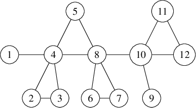
Since
 $\Gamma $
has three cut edges
$\Gamma $
has three cut edges
 $(1,4)$
,
$(1,4)$
,
 $(8,10)$
, and
$(8,10)$
, and
 $(9,10)$
, we have that
$(9,10)$
, we have that
 $$\begin{align*}\mathcal{C}_\Gamma =\left\{\bar{f}_A^{(1,4)} \mid A \subset [12],\, \left| A \right| =1 \right\} \cup \left\{\bar{f}_A^{(8,10)} \mid A \subset [12],\, \left| A \right| =8 \right\} \cup \left\{\bar{f}_A^{(9,10)} \mid A \subset [12],\, \left| A \right| =1 \right\}.\end{align*}$$
One such element
 $\bar {f}_{\{6\}}^{(9,10)} \in \mathcal {C}_\Gamma $
takes the form
$\bar {f}_{\{6\}}^{(9,10)} \in \mathcal {C}_\Gamma $
takes the form
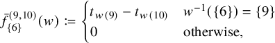
and is supported on the coset
 $\{w \in S_n \mid w(9) = 6\}$
.
$\{w \in S_n \mid w(9) = 6\}$
.
Since
 $\Gamma $
has three cut vertices
$\Gamma $
has three cut vertices
 $4$
,
$4$
,
 $8$
, and
$8$
, and
 $10$
, we have that
$10$
, we have that
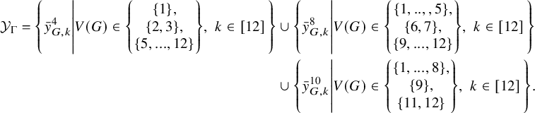 $$ \begin{align*} \mathcal{Y}_\Gamma=\left\{\bar{y}_{G,k}^4 \left| V(G) \in \left\{ \begin{matrix} \{1 \}, \\ \{2,3 \}, \\ \{5,...,12 \} \end{matrix} \right\},\; k \in [12] \right.\right\}&\cup \left\{\bar{y}_{G,k}^8 \left| V(G) \in \left\{ \begin{matrix} \{1,..,,5 \}, \\ \{6,7 \}, \\ \{9,...,12 \} \end{matrix} \right\},\; k \in [12] \right.\right\} \\&\cup \left\{\bar{y}_{G,k}^{10} \left| V(G) \in \left\{ \begin{matrix} \{1,...,8 \}, \\ \{9 \}, \\ \{11,12 \} \end{matrix} \right\},\; k \in [12] \right.\right\}. \end{align*} $$
One such element
 $\bar {y}_{G,3}^8 \in \mathcal {Y}_\Gamma $
takes the form
$\bar {y}_{G,3}^8 \in \mathcal {Y}_\Gamma $
takes the form
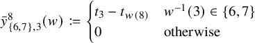
and is supported on the set
 $\{w \in S_n \mid w(6) = 3 \text { or } w(7) = 3\}$
.
$\{w \in S_n \mid w(6) = 3 \text { or } w(7) = 3\}$
.
Now Lemma 5.3 below shows that
 $\mathcal {F}_\Gamma $
is in fact a subset of
$\mathcal {F}_\Gamma $
is in fact a subset of
 $\mathcal {M}_{\Gamma }^1$
.
$\mathcal {M}_{\Gamma }^1$
.
Lemma 5.3. Let
 $\Gamma $
be a graph on
$\Gamma $
be a graph on
 $[n]$
. The four sets
$[n]$
. The four sets
 $\mathcal {T}_n$
,
$\mathcal {T}_n$
,
 $\mathcal {X}_n$
,
$\mathcal {X}_n$
,
 $\mathcal {C}_\Gamma $
and
$\mathcal {C}_\Gamma $
and
 $\mathcal {Y}_\Gamma $
are subsets of
$\mathcal {Y}_\Gamma $
are subsets of
 $\mathcal {M}_{\Gamma }$
.
$\mathcal {M}_{\Gamma }$
.
Proof. We already know that
 $\bar {t}_i$
and
$\bar {t}_i$
and
 $\bar {x}_i$
are elements of
$\bar {x}_i$
are elements of
 $\mathcal {M}_{\Gamma }$
for all
$\mathcal {M}_{\Gamma }$
for all
 $i \in [n]$
, so
$i \in [n]$
, so
 $\mathcal {T}_n$
and
$\mathcal {T}_n$
and
 $\mathcal {X}_n$
are subsets.
$\mathcal {X}_n$
are subsets.
Now we show that each element of
 $\mathcal {C}_\Gamma $
is a well-defined spline. Recall that these are coset splines, and so are well defined for trees. If s is a cut edge of
$\mathcal {C}_\Gamma $
is a well-defined spline. Recall that these are coset splines, and so are well defined for trees. If s is a cut edge of
 $\Gamma $
, then every spanning tree T of
$\Gamma $
, then every spanning tree T of
 $\Gamma $
must have s as an edge. Fix
$\Gamma $
must have s as an edge. Fix
 $A \subset [n]$
, where
$A \subset [n]$
, where
 $\left | A \right | = \left | G_s \right |$
, and for all spanning trees T, choose
$\left | A \right | = \left | G_s \right |$
, and for all spanning trees T, choose
 $T_s$
to be the connected component where
$T_s$
to be the connected component where
 $V(T_s) = V(G_s)$
. It follows that
$V(T_s) = V(G_s)$
. It follows that
 $\bar {f}_A^s \in \mathcal {M}_{T}$
for every spanning tree T, and so
$\bar {f}_A^s \in \mathcal {M}_{T}$
for every spanning tree T, and so
 $\bar {f}_A^s \in \mathcal {M}_{\Gamma }$
by Lemma 2.16.
$\bar {f}_A^s \in \mathcal {M}_{\Gamma }$
by Lemma 2.16.
Finally, we show that every element
 $\bar {y}_{G,k}^j \in \mathcal {Y}_\Gamma $
is a linear spline on
$\bar {y}_{G,k}^j \in \mathcal {Y}_\Gamma $
is a linear spline on
 $\mathcal {G}_\Gamma $
. We will verify this from the definition, edge by edge. Let
$\mathcal {G}_\Gamma $
. We will verify this from the definition, edge by edge. Let
 $(w,v) \in E(\mathcal {G}_\Gamma )$
, where
$(w,v) \in E(\mathcal {G}_\Gamma )$
, where
 $w = v(p,q)$
. We prove that
$w = v(p,q)$
. We prove that
 $\bar {y}_{G,k}^j(w)-\bar {y}_{G,k}^j(v) \in \mathcal {L}(w,v) = \left \langle t_{v(p)} - t_{v(q)}\right \rangle $
in three cases, depending on the values of
$\bar {y}_{G,k}^j(w)-\bar {y}_{G,k}^j(v) \in \mathcal {L}(w,v) = \left \langle t_{v(p)} - t_{v(q)}\right \rangle $
in three cases, depending on the values of
 $w^{-1}(k)$
and
$w^{-1}(k)$
and
 $v^{-1}(k)$
.
$v^{-1}(k)$
.
Case 1:
 $w^{-1}(k),v^{-1}(k) \notin G$
. Then by definition both
$w^{-1}(k),v^{-1}(k) \notin G$
. Then by definition both
 $\bar {y}_{G,k}^j(w) = 0$
and
$\bar {y}_{G,k}^j(w) = 0$
and
 $\bar {y}_{G,k}^j(v) = 0$
, so the difference is clearly in
$\bar {y}_{G,k}^j(v) = 0$
, so the difference is clearly in
 $\mathcal {L}(w,v)$
.
$\mathcal {L}(w,v)$
.
Case 2:
 $w^{-1}(k),v^{-1}(k) \in G$
. So
$w^{-1}(k),v^{-1}(k) \in G$
. So
 $\bar {y}_{G,k}^j$
contains both w and v in its support. We compute from the definition that
$\bar {y}_{G,k}^j$
contains both w and v in its support. We compute from the definition that
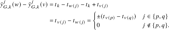 $$ \begin{align*} \bar{y}_{G,k}^j(w)-\bar{y}_{G,k}^j(v) &= t_k-t_{w(j)}-t_k+t_{v(j)} \\ &= t_{v(j)} - t_{w(j)} = \begin{cases} \pm(t_{v(p)} - t_{v(q)}) & j\in \{p,q\} \\ 0 & j \notin \{p,q\}. \end{cases} \end{align*} $$
In either case, this difference is in the ideal
 $\mathcal {L}(w,v)$
.
$\mathcal {L}(w,v)$
.
Case 3:
 $w^{-1}(k) \in G$
,
$w^{-1}(k) \in G$
,
 $v^{-1}(k) \notin G$
. In particular, w is in the support of
$v^{-1}(k) \notin G$
. In particular, w is in the support of
 $\bar {y}_{G,k}^j$
whereas v is not. Since
$\bar {y}_{G,k}^j$
whereas v is not. Since
 $w^{-1}(k) = (p,q)v^{-1}(k)$
, we know that one of either p or q is in G and the other is not. Without loss of generality, say
$w^{-1}(k) = (p,q)v^{-1}(k)$
, we know that one of either p or q is in G and the other is not. Without loss of generality, say
 $p \in G$
and
$p \in G$
and
 $q \notin G$
. In particular,
$q \notin G$
. In particular,
 $w^{-1}(k) = p$
and
$w^{-1}(k) = p$
and
 $v^{-1}(k) = q$
. Since
$v^{-1}(k) = q$
. Since
 $(p,q) \in E(\Gamma )$
and the only element in
$(p,q) \in E(\Gamma )$
and the only element in
 $[n] \setminus V(G)$
that elements of G are connected to is the vertex j, it follows that
$[n] \setminus V(G)$
that elements of G are connected to is the vertex j, it follows that
 $v^{-1}(k) = q = j$
. So
$v^{-1}(k) = q = j$
. So
 $v(q) = k$
and
$v(q) = k$
and
 $w(j) = v(p,q)(j) = v(p)$
. Compute that
$w(j) = v(p,q)(j) = v(p)$
. Compute that
 $$\begin{align*}\bar{y}_{G,k}^j(w)-\bar{y}_{G,k}^j(v) = t_k-t_{w(j)} = t_{v(q)} - t_{v(p,q)(j)} = t_{v(q)} - t_{v(p)} \in \mathcal{L}(w,v). \end{align*}$$
Thus,
 $\bar {y}_{G,k}^j$
is an element of
$\bar {y}_{G,k}^j$
is an element of
 $\mathcal {M}_{\Gamma }$
.
$\mathcal {M}_{\Gamma }$
.
The splines in
 $\mathcal {F}_\Gamma $
are defined from graph properties that are intrinsic to the isomorphism class of
$\mathcal {F}_\Gamma $
are defined from graph properties that are intrinsic to the isomorphism class of
 $\Gamma $
. Lemma 5.4 below makes this precise.
$\Gamma $
. Lemma 5.4 below makes this precise.
Lemma 5.4. Let
 $\omega \colon \Gamma \to \Gamma '$
be a graph isomorphism and
$\omega \colon \Gamma \to \Gamma '$
be a graph isomorphism and
 $\Omega $
be as in Subsection 2.3. Then
$\Omega $
be as in Subsection 2.3. Then
 $\mathcal {F}_{\Gamma '} = \Omega \left (\mathcal {F}_{\Gamma }\right )$
.
$\mathcal {F}_{\Gamma '} = \Omega \left (\mathcal {F}_{\Gamma }\right )$
.
Proof. It follows directly from the definitions that
 $\Omega (\mathcal {X}_n) = \mathcal {X}_n$
and
$\Omega (\mathcal {X}_n) = \mathcal {X}_n$
and
 $\Omega (\mathcal {T}_n) = \mathcal {T}_n$
.
$\Omega (\mathcal {T}_n) = \mathcal {T}_n$
.
The image of the coset spline
 $\bar {f}_A^{(i,j)} \in \mathcal {M}_{\Gamma }$
can be computed to be the coset spline
$\bar {f}_A^{(i,j)} \in \mathcal {M}_{\Gamma }$
can be computed to be the coset spline
 $\bar {f}_{w^{-1}(A)}^{(w(i),w(j))} \in \mathcal {M}_{\Gamma '}$
, where we consistently choose the connected component
$\bar {f}_{w^{-1}(A)}^{(w(i),w(j))} \in \mathcal {M}_{\Gamma '}$
, where we consistently choose the connected component
 $\omega (G_s)$
. From this, it is straightforward from the definitions to verify that
$\omega (G_s)$
. From this, it is straightforward from the definitions to verify that
 $\mathcal {C}_{\Gamma '} = \Omega (\mathcal {C}_\Gamma )$
Similarly, it is easy to verify that
 $\bar {y}_{G,k}^j \mapsto \bar {y}_{w(G),w(k)}^{w(j)}$
, and so
$\bar {y}_{G,k}^j \mapsto \bar {y}_{w(G),w(k)}^{w(j)}$
, and so
 $\mathcal {Y}_{\Gamma '} = \Omega (\mathcal {Y}_\Gamma )$
.
$\mathcal {Y}_{\Gamma '} = \Omega (\mathcal {Y}_\Gamma )$
.
By Lemma 5.4, it suffices to prove that
 $\mathcal {F}_\Gamma $
spans
$\mathcal {F}_\Gamma $
spans
 $\mathcal {M}_{\Gamma }^1$
for any particular graph in isomorphism class of
$\mathcal {M}_{\Gamma }^1$
for any particular graph in isomorphism class of
 $\Gamma $
.
$\Gamma $
.
5.1 Some relations
This set
 $\mathcal {F}_\Gamma $
is not a
$\mathcal {F}_\Gamma $
is not a
 $\mathbb {C}$
-basis of
$\mathbb {C}$
-basis of
 $\mathcal {M}_{\Gamma }^1$
. Indeed, the following Lemmas 5.5, 5.6 and 5.7 give relations between elements of
$\mathcal {M}_{\Gamma }^1$
. Indeed, the following Lemmas 5.5, 5.6 and 5.7 give relations between elements of
 $\mathcal {F}_\Gamma $
.
$\mathcal {F}_\Gamma $
.
The first set of relations in the Lemma 5.5 are relatively straightforward.
Lemma 5.5. For
 $\bar {t}_i \in \mathcal {T}_n$
,
$\bar {t}_i \in \mathcal {T}_n$
,
 $\bar {x}_i\in \mathcal {X}_n$
,
$\bar {x}_i\in \mathcal {X}_n$
,
 $\bar {f}_A^s\in \mathcal {F}_\Gamma $
and
$\bar {f}_A^s\in \mathcal {F}_\Gamma $
and
 $\bar {y}_{G,k}^j \in \mathcal {Y}_\Gamma $
, the following relations hold:
$\bar {y}_{G,k}^j \in \mathcal {Y}_\Gamma $
, the following relations hold:
-
(1)
${ \sum\limits _{r=1}^n \bar {x}_r = \sum\limits _{r=1}^n \bar {t}_r }$
, -
(2) if
$(i,j)$
is a cut edge and
$G_{(i,j)}$
is the component containing the vertex i, then
${ \sum\limits _{A} \bar {f}_A^{(i,j)} = \bar {x}_i - \bar {x}_j}$
, where the sum is over all
$A \subset [n]$
such that
$\left | A \right | = \left | G_{(i,j)} \right |$
, -
(3) if
$j \vdash \Gamma $
, then
${ \sum\limits _{k=1}^n \bar {y}_{G,k}^j = \left (\sum\limits _{r\in G} \bar {x}_r\right ) - \left | G \right |\bar {x}_j}$
for any connected component G of
$\Gamma - j$
, and -
(4) if
$j \vdash \Gamma $
and
$k \in [n]$
is fixed,
${ \sum\limits _{G} \bar {y}_{G,k}^i = \bar {t}_k - \bar {x}_j}$
, where the sum is over all connected components G of
$\Gamma - j$
.


Proof. Relation
 $(1)$
is easy, as is relation
$(1)$
is easy, as is relation
 $(2)$
once it is noted that the support of each
$(2)$
once it is noted that the support of each
 $\bar {f}_A^{(i,j)}$
for a fixed
$\bar {f}_A^{(i,j)}$
for a fixed
 $(i,j)$
is disjoint. Fix
$(i,j)$
is disjoint. Fix
 $w \in S_n$
.
$w \in S_n$
.
For relation (3), compute that
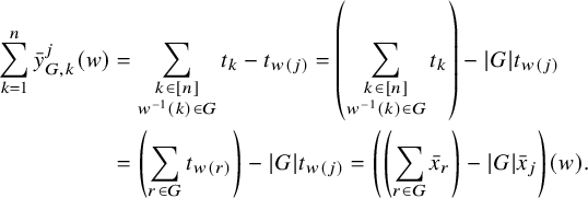 $$ \begin{align*} \sum_{k=1}^n \bar{y}_{G,k}^j(w) &= \sum_{\substack{k \in [n]\\w^{-1}(k) \in G}} t_k - t_{w(j)} = \left(\sum_{\substack{k\in [n]\\w^{-1}(k) \in G}} t_k\right) - \left| G \right|t_{w(j)} \\ &= \left(\sum_{r \in G} t_{w(r)}\right) - \left| G \right|t_{w(j)} = \left(\left(\sum_{r\in G} \bar{x}_r\right) - \left| G \right|\bar{x}_j\right)(w). \end{align*} $$
For relation (4), note that either
 $w^{-1}(k) = j$
or
$w^{-1}(k) = j$
or
 $w^{-1}(k) \in G$
for one and only one connected component G of
$w^{-1}(k) \in G$
for one and only one connected component G of
 $\Gamma - j$
. As such, if
$\Gamma - j$
. As such, if
 $w^{-1}(k) = j$
, in which case w is not in the support of any of the
$w^{-1}(k) = j$
, in which case w is not in the support of any of the
 $\bar {y}_{G,k}^j$
and likewise
$\bar {y}_{G,k}^j$
and likewise
 $\bar {t}_k(w)-\bar {x}_j(w) = 0$
. Otherwise,
$\bar {t}_k(w)-\bar {x}_j(w) = 0$
. Otherwise,
 $w^{-1}(k) \in G$
for some particular connected component G and
$w^{-1}(k) \in G$
for some particular connected component G and
 $\bar {y}_{G,k}^j(w) = t_k-t_{w(j)}$
. This is precisely
$\bar {y}_{G,k}^j(w) = t_k-t_{w(j)}$
. This is precisely
 $\bar {t}_k(w) - \bar {x}_j(w)$
, and we have (4).
$\bar {t}_k(w) - \bar {x}_j(w)$
, and we have (4).
Lemma 5.6 below shows that if j is a cut vertex and a connected component G of
 $\Gamma - j$
is connected to j by a cut edge
$\Gamma - j$
is connected to j by a cut edge
 $(i,j)$
, then the spline
$(i,j)$
, then the spline
 $\bar {y}_{G,k}^j$
can be written as a sum of other splines from
$\bar {y}_{G,k}^j$
can be written as a sum of other splines from
 $\mathcal {F}_\Gamma $
. In particular, it will allow us to remove from
$\mathcal {F}_\Gamma $
. In particular, it will allow us to remove from
 $\mathcal {F}_\Gamma $
the splines in
$\mathcal {F}_\Gamma $
the splines in
 $\mathcal {Y}_\Gamma $
that correspond to components connected by cut edges.
$\mathcal {Y}_\Gamma $
that correspond to components connected by cut edges.
Lemma 5.6. Let
 $\Gamma $
be a graph, j a cut vertex and
$\Gamma $
be a graph, j a cut vertex and
 $(i,j)$
a cut edge, choosing
$(i,j)$
a cut edge, choosing
 $G_{(i,j)}$
to be the component containing the vertex i. Let C be the connected component of the forest with vertex set
$G_{(i,j)}$
to be the component containing the vertex i. Let C be the connected component of the forest with vertex set
 $V(G_{(i,j)}) \cup \{j\}$
and edge set
$V(G_{(i,j)}) \cup \{j\}$
and edge set
 $\{s \mid s\text { is a cut edge of }G_{(i,j)}\} \cup \{(i,j)\}$
that contains the vertex j. Then for all
$\{s \mid s\text { is a cut edge of }G_{(i,j)}\} \cup \{(i,j)\}$
that contains the vertex j. Then for all
 $k \in [n]$
,
$k \in [n]$
,
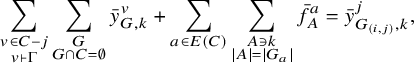 $$\begin{align*}\sum_{\substack{v \in C-j \\v \vdash \Gamma}} \sum_{\substack{ G\\ G \cap C = \emptyset}} \bar{y}_{G,k}^v + \sum_{a \in E(C)} \sum_{\substack{A \ni k\\ \left| A \right| = \left| G_a \right|}} \bar{f}_A^{a} = \bar{y}_{G_{(i,j)},k}^j, \end{align*}$$
where G in the first double-sum is a connected component of
 $\Gamma - v$
, where
$\Gamma - v$
, where
 $G_a$
is the connected component that is a subset of
$G_a$
is the connected component that is a subset of
 $G_{(i,j)}$
, and where A in the second double-sum is a subset of
$G_{(i,j)}$
, and where A in the second double-sum is a subset of
 $[n]$
.
$[n]$
.
Since Lemma 5.6 is rather technical, we will walk through an example before seeing the full proof. Let
 $\Gamma $
be the graph on
$\Gamma $
be the graph on
 $13$
vertices below:
$13$
vertices below:
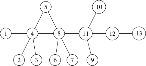
where
 $(11,12)$
is cut edge and
$(11,12)$
is cut edge and
 $G_{(11,12)}$
is the component that contains
$G_{(11,12)}$
is the component that contains
 $11$
. The forest of cut edges with vertex set
$11$
. The forest of cut edges with vertex set
 $V(G_{(11,12)}) \cup \{12\}$
has edge set
$V(G_{(11,12)}) \cup \{12\}$
has edge set
 $\{(1,4),(8,11),(9,11),(10,11),(12,11)\}$
. If we mark in
$\{(1,4),(8,11),(9,11),(10,11),(12,11)\}$
. If we mark in
 $\Gamma $
the component of this forest that contains the vertex
$\Gamma $
the component of this forest that contains the vertex
 $11$
with double lines, we get the following graph:
$11$
with double lines, we get the following graph:

In essence, Lemma 5.6 says that for all
 $k \in [13]$
, the spline
$k \in [13]$
, the spline
 $\bar {y}_{G_{(11,12)},k}^{12}$
can be written as a sum of some splines in
$\bar {y}_{G_{(11,12)},k}^{12}$
can be written as a sum of some splines in
 $\mathcal {C}_\Gamma $
associated to the cut edges
$\mathcal {C}_\Gamma $
associated to the cut edges
 $(8,11)$
,
$(8,11)$
,
 $(9,11)$
and
$(9,11)$
and
 $(10,11)$
(since they are a part of that marked tree) and some splines in
$(10,11)$
(since they are a part of that marked tree) and some splines in
 $\mathcal {Y}_\Gamma $
associated to cut vertex
$\mathcal {Y}_\Gamma $
associated to cut vertex
 $8$
, since
$8$
, since
 $\Gamma - 8$
has components that ‘hang off of’ that marked tree.
$\Gamma - 8$
has components that ‘hang off of’ that marked tree.
For each of the cut edges
 $a \in \{(8,11),(9,11),(10,11)\}$
, we must choose
$a \in \{(8,11),(9,11),(10,11)\}$
, we must choose
 $G_a$
to be the component contained within
$G_a$
to be the component contained within
 $G_{(11,12)}$
, so
$G_{(11,12)}$
, so
 $V(G_{(9,11)}) = \{1,...,11\}$
,
$V(G_{(9,11)}) = \{1,...,11\}$
,
 $V(G_{(9,11)}) = \{9\}$
, and
$V(G_{(9,11)}) = \{9\}$
, and
 $V(G_{(10,11)}) = \{10\}$
.
$V(G_{(10,11)}) = \{10\}$
.
More formally, Lemma 5.6 states that for all
 $k \in [13]$
, the following equality holds (we will denote the specific subgraph by their vertex set):
$k \in [13]$
, the following equality holds (we will denote the specific subgraph by their vertex set):
 $$\begin{align*}\bar{y}_{[5],k}^8 + \bar{y}_{\{6,7\},k}^8 + \sum_{\substack{\left| A \right| = 8 \\ k \in A}} \bar{f}_A^{(8,11)}+ \sum_{\substack{\left| A \right| = 1 \\ k \in A}} \bar{f}_A^{(9,11)}+ \sum_{\substack{\left| A \right| = 1 \\ k \in A}} \bar{f}_A^{(10,11)}+ \sum_{\substack{\left| A \right| = 11 \\ k \in A}} \bar{f}_A^{(11,12)} = \bar{y}_{[11],k}^{12}.\end{align*}$$
The proof proceeds in cases by the value of
 $w^{-1}(k)$
. For example, say we wished to evaluate both sides of the above expression at a
$w^{-1}(k)$
. For example, say we wished to evaluate both sides of the above expression at a
 $w \in S_{13}$
such that
$w \in S_{13}$
such that
 $w^{-1}(k) = 3$
. This makes it easier to determine which splines in the sum above on the left are supported at w. In particular,
$w^{-1}(k) = 3$
. This makes it easier to determine which splines in the sum above on the left are supported at w. In particular,
-
1.
${ \bar {y}_{[5],k}^8(w) = t_k - t_{w(8)}}$
since
$3 \in [5]$
, -
2.
${ \bar {y}_{\{6,7\},k}^8(w) = 0}$
since
$3 \notin \{6,7\}$
, -
3.
${ \sum _{\substack {\left | A \right | = 8 \\ k \in A}} \bar {f}_A^{(8,11)}(w) = t_{w(8)} - t_{w(11)}}$
since the set
$A = w(V(G_{(8,11)})$
contains
$w(3) = k$
, -
4.
${ \sum _{\substack {\left | A \right | = 1 \\ k \in A}} \bar {f}_A^{(9,11)}(w) = 0}$
and
${ \sum _{\substack {\left | A \right | = 1 \\ k \in A}} \bar {f}_A^{(10,11)}(w) = 0}$
since
$k \notin w(\{9\})$
and
$k\notin w(\{10\})$
, and finally, -
5.
${ \sum _{\substack {\left | A \right | = 11 \\ k \in A}} \bar {f}_A^{(11,12)}(w) = t_{w(11)} - t_{w(12)}}$
since the set
$A = w(V(G_{(11,12)})$
contains
$w(3) = k$
.


If we add these all up, the sum telescopes and the evaluation is
 $$\begin{align*}(t_k - t_{w(8)}) + (t_{w(8)} - t_{w(11))} + (t_{w(11)} - t_{w(12)}) = t_k - t_{w(12)},\end{align*}$$
which is precisely
 ${ \bar {y}_{[11]}^{12}(w)}$
. The essence of the proof, which we will now provide, is that the splines in the sum with support at a particular
${ \bar {y}_{[11]}^{12}(w)}$
. The essence of the proof, which we will now provide, is that the splines in the sum with support at a particular
 $w \in S_n$
can be determined from any simple path from
$w \in S_n$
can be determined from any simple path from
 $w^{-1}(k)$
to j and that the sum always telescopes as it did in the example above.
$w^{-1}(k)$
to j and that the sum always telescopes as it did in the example above.
Proof of Lemma 5.6.
Let
 $w \in S_n$
. We will show that both sides of the claimed equality are equal when evaluated at w. Let
$w \in S_n$
. We will show that both sides of the claimed equality are equal when evaluated at w. Let
 $k \in [n]$
, and we will proceed in cases based off of the value
$k \in [n]$
, and we will proceed in cases based off of the value
 $w^{-1}(k)$
.
$w^{-1}(k)$
.
First, say
 $w^{-1}(k) \notin V(G_{(i,j)})$
. All paths that begin in
$w^{-1}(k) \notin V(G_{(i,j)})$
. All paths that begin in
 $G_{(i,j)}$
and leave must contain the edge
$G_{(i,j)}$
and leave must contain the edge
 $(i,j)$
and thus visit the vertex j. In particular, for any
$(i,j)$
and thus visit the vertex j. In particular, for any
 $v \in C$
where
$v \in C$
where
 $c \vdash \Gamma $
, the connected component of
$c \vdash \Gamma $
, the connected component of
 $\Gamma - v$
that contains
$\Gamma - v$
that contains
 $w^{-1}(k)$
also contains
$w^{-1}(k)$
also contains
 $j \in C$
. So
$j \in C$
. So
 $w^{-1}(k) \notin G$
for any G in the first double-sum, and so
$w^{-1}(k) \notin G$
for any G in the first double-sum, and so
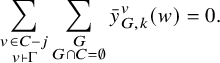 $$\begin{align*}\sum_{\substack{v \in C-j \\v \vdash \Gamma}} \sum_{\substack{ G\\ G \cap C = \emptyset}} \bar{y}_{G,k}^v(w) = 0.\end{align*}$$
If
 $a \in E(C)$
, then
$a \in E(C)$
, then
 $G_a$
was chosen to be contained within
$G_a$
was chosen to be contained within
 $G_{(i,j)}$
, so
$G_{(i,j)}$
, so
 $w^{-1}(k) \notin G_a$
as well. In particular, if
$w^{-1}(k) \notin G_a$
as well. In particular, if
 $k \in A$
, then
$k \in A$
, then
 $w^{-1}(A) \neq G_a$
, and so
$w^{-1}(A) \neq G_a$
, and so
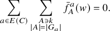 $$\begin{align*}\sum_{a \in E(C)} \sum_{\substack{A \ni k\\\left| A \right| = \left| G_a \right|}} \bar{f}_A^{a}(w) = 0.\end{align*}$$
It is direct from the definition that
 $\bar {y}_{G_{(i,j)},k}^v(w) = 0$
, and so the claim holds when
$\bar {y}_{G_{(i,j)},k}^v(w) = 0$
, and so the claim holds when
 $w^{-1}(k) \notin G_{(i,j)}$
.
$w^{-1}(k) \notin G_{(i,j)}$
.
Now assume that
 $w^{-1}(k) \in G_{(i,j)}$
. Let
$w^{-1}(k) \in G_{(i,j)}$
. Let
 $P = \left (p_0,\ldots ,p_\ell , p_{\ell +1} \right )$
be a simple path from
$P = \left (p_0,\ldots ,p_\ell , p_{\ell +1} \right )$
be a simple path from ![]() to
to ![]() . Note that
. Note that
 $p_\ell $
must be the vertex i. This path P may start outside of C, but must eventually enter the tree C. Say that
$p_\ell $
must be the vertex i. This path P may start outside of C, but must eventually enter the tree C. Say that
 $m \in \{0,...,\ell \}$
is the lowest index such that
$m \in \{0,...,\ell \}$
is the lowest index such that
 $p_m \in C$
. Since
$p_m \in C$
. Since
 $i \in C$
and
$i \in C$
and
 $p_\ell = i$
, this integer m does exist. Simple paths from vertex to vertex within trees are unique, so there is a unique simple path from
$p_\ell = i$
, this integer m does exist. Simple paths from vertex to vertex within trees are unique, so there is a unique simple path from
 $p_m$
to j in C. This path is
$p_m$
to j in C. This path is ![]() .
.
First, we will determine the value of
 $\bar {f}_A^{a}(w)$
for
$\bar {f}_A^{a}(w)$
for
 $a \in E(C)$
. Say the edge
$a \in E(C)$
. Say the edge
 $a \in C$
is not an edge in the path
$a \in C$
is not an edge in the path
 $P^C$
. Then the vertices
$P^C$
. Then the vertices
 $w^{-1}(k)$
and j are in the same connected component of the graph
$w^{-1}(k)$
and j are in the same connected component of the graph
 $([n],E(\Gamma )-a)$
. In particular,
$([n],E(\Gamma )-a)$
. In particular,
 $w^{-1}(k) \notin G_a$
, so if
$w^{-1}(k) \notin G_a$
, so if
 $k \in A$
, then
$k \in A$
, then
 $w^{-1}(A) \neq V(G_a)$
. It follows that for all A such that
$w^{-1}(A) \neq V(G_a)$
. It follows that for all A such that
 $k \in A$
, if
$k \in A$
, if
 $a \notin P^C$
, then
$a \notin P^C$
, then
 $\bar {f}_A^{a}(w) = 0$
.
$\bar {f}_A^{a}(w) = 0$
.
However, if
 $a \in P^C$
, then we may let
$a \in P^C$
, then we may let ![]() , and then
, and then
 $k \in A$
. So for each
$k \in A$
. So for each
 $a \in P^C$
, there exists a single spline
$a \in P^C$
, there exists a single spline
 $\bar {f}_A^{a}$
in the sum that is supported at w. In particular, if
$\bar {f}_A^{a}$
in the sum that is supported at w. In particular, if
 $a = (p,q)$
, then
$a = (p,q)$
, then
 $\bar {f}_A^{q}(w) = t_{w(p)} - t_{w(q)}$
.
$\bar {f}_A^{q}(w) = t_{w(p)} - t_{w(q)}$
.
At this point, we have that
 $$\begin{align*}\sum_{\substack{v \in C-j \\v \vdash \Gamma}} \sum_{\substack{ G\\ G \cap C = \emptyset}} \bar{y}_{G,k}^v(w) + \sum_{a \in E(C)} \sum_{\substack{A \ni k\\\left| A \right| = \left| G_a \right|}} \bar{f}_A^{a} = \sum_{\substack{v \in C-j \\v \vdash \Gamma}} \sum_{\substack{ G\\ G \cap C = \emptyset}} \bar{y}_{G,k}^v(w) + \sum_{(p,q) \in P^C} t_{w(p)} - t_{w(q)}. \end{align*}$$
Now we will have two cases: if
 $w^{-1}(k) \in C$
and if
$w^{-1}(k) \in C$
and if
 $w^{-1}(k) \notin C$
.
$w^{-1}(k) \notin C$
.
Case 1:
 $w^{-1}(k) \in C$
. So
$w^{-1}(k) \in C$
. So
 $m = 0$
. Then for all
$m = 0$
. Then for all
 $v \in G_{(i,j)}$
, if a connected component G of
$v \in G_{(i,j)}$
, if a connected component G of
 $\Gamma - v$
contains
$\Gamma - v$
contains
 $w^{-1}(k)$
, then so does
$w^{-1}(k)$
, then so does
 $G \cap C$
. In particular,
$G \cap C$
. In particular,
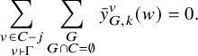 $$\begin{align*}\sum_{\substack{v \in C-j \\v \vdash \Gamma}} \sum_{\substack{ G\\ G \cap C = \emptyset}} \bar{y}_{G,k}^v(w) = 0.\end{align*}$$
Now we compute
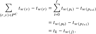 $$ \begin{align*} \sum_{(r,v) \in P^C} t_{w(v)} - t_{w(r)} &=\sum_{i=0}^\ell t_{w(p_i)} - t_{w(p_{i+1})} \\ &= t_{w(p_0)} - t_{w(p_{\ell+1})}\\ &= t_k - t_{w(j)}. \end{align*} $$
This is precisely
 $\bar {y}_i^j(w)$
, and so the equality holds if
$\bar {y}_i^j(w)$
, and so the equality holds if
 $w^{-1}(k) \in C$
.
$w^{-1}(k) \in C$
.
Case 2:
 $w^{-1}(k) \notin C$
. Then
$w^{-1}(k) \notin C$
. Then
 $m \neq 0$
, and consider the vertex
$m \neq 0$
, and consider the vertex
 $p_{m-1}$
. Since
$p_{m-1}$
. Since
 $p_m \in C$
and
$p_m \in C$
and
 $\Gamma - p_m$
separates
$\Gamma - p_m$
separates
 $w^{-1}(k)$
from j, the vertex
$w^{-1}(k)$
from j, the vertex
 $p_m$
is a cut vertex of
$p_m$
is a cut vertex of
 $\Gamma $
. If
$\Gamma $
. If
 $v' \in C$
is any vertex other than
$v' \in C$
is any vertex other than
 $p_m$
, then
$p_m$
, then
 $p_m$
and
$p_m$
and
 $w^{-1}(k)$
are in the same connected component of
$w^{-1}(k)$
are in the same connected component of
 $\Gamma - v'$
(connected via the path
$\Gamma - v'$
(connected via the path
 $(p_0,...,p_m)$
). In particular, any connected component of
$(p_0,...,p_m)$
). In particular, any connected component of
 $\Gamma - v'$
that contains
$\Gamma - v'$
that contains
 $w^{-1}(k)$
intersects nontrivially with C. So for
$w^{-1}(k)$
intersects nontrivially with C. So for
 $v=p_m \in C-j$
, there is precisely one component G of
$v=p_m \in C-j$
, there is precisely one component G of
 $\Gamma - v$
that contains
$\Gamma - v$
that contains
 $w^{-1}(k)$
. If this component G intersected nontrivially with C, then
$w^{-1}(k)$
. If this component G intersected nontrivially with C, then
 $(p_{m-1},p_m)$
would have to be an edge in C, but
$(p_{m-1},p_m)$
would have to be an edge in C, but
 $(p_{m-1},p_m)$
was explicitly assumed not to be a cut edge. In particular, w is supported on one and only one spline in the first double-sum (the one where
$(p_{m-1},p_m)$
was explicitly assumed not to be a cut edge. In particular, w is supported on one and only one spline in the first double-sum (the one where
 $v = p_m$
and
$v = p_m$
and
 $G \ni p_{m-1})$
), and so
$G \ni p_{m-1})$
), and so
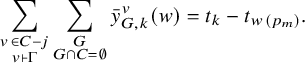 $$\begin{align*}\sum_{\substack{v \in C-j \\v \vdash \Gamma}} \sum_{\substack{ G\\ G \cap C = \emptyset}} \bar{y}_{G,k}^v(w) = t_k - t_{w(p_m)}. \end{align*}$$
It follows that
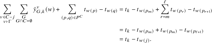 $$ \begin{align*} \sum_{\substack{v \in C-j \\v \vdash \Gamma}} \sum_{\substack{ G\\ G \cap C = \emptyset}} \bar{y}_{G,k}^v(w) + \sum_{(p,q) \in P^C} t_{w(p)} - t_{w(q)} &= t_k - t_{w(p_m)} + \sum_{r=m}^\ell t_{w(p_r)} - t_{w(p_{r+1})} \\ &= t_{k} - t_{w(p_m)} + t_{w(p_m)} - t_{w(p_{\ell+1})}\\ &= t_k - t_{w(j)}. \end{align*} $$
So in either case, the sum evaluates to
 $\bar {y}_{G_{(i,j)},k}^j(w)$
.
$\bar {y}_{G_{(i,j)},k}^j(w)$
.
Now Lemma 5.6 two very important consequences. First, as mentioned, it will allow us to disregard those splines
 $\bar {y}_{G,k}^j$
where G is connected to j via a cut edge. Second, observe we only required j to be a cut vertex so that
$\bar {y}_{G,k}^j$
where G is connected to j via a cut edge. Second, observe we only required j to be a cut vertex so that
 $\bar {y}_{G,k}^j$
is defined. We may, however, remove this restriction and ‘force through’ the argument as follows. If
$\bar {y}_{G,k}^j$
is defined. We may, however, remove this restriction and ‘force through’ the argument as follows. If
 $(p,q)$
is a cut edge and q is not a cut vertex, then q is a leaf in
$(p,q)$
is a cut edge and q is not a cut vertex, then q is a leaf in
 $\Gamma $
. Let
$\Gamma $
. Let
 $G_{(p,q)}$
be the connected component containing p (and thereby all of
$G_{(p,q)}$
be the connected component containing p (and thereby all of
 $[n] \setminus \{q\}$
). We might abuse notation and let for all
$[n] \setminus \{q\}$
). We might abuse notation and let for all
 $w \in S_n$
,
$w \in S_n$
,
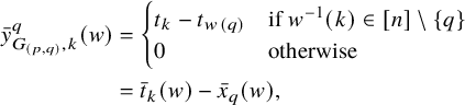 $$ \begin{align*} \bar{y}_{G_{(p,q)},k}^q(w) &= \begin{cases} t_k - t_{w(q)} & \text{if }w^{-1}(k) \in [n] \setminus\{q\} \\ 0 &\text{otherwise} \end{cases} \\ &= \bar{t}_k(w) - \bar{x}_q(w), \end{align*} $$
and get another relation from Lemma 5.6. A consequence of this is Lemma 5.7 below.
Lemma 5.7. Let
 $(i,j)$
be a leaf edge in
$(i,j)$
be a leaf edge in
 $\Gamma $
with j the leaf vertex, and
$\Gamma $
with j the leaf vertex, and
 $G_{(i,j)}$
the connected component of
$G_{(i,j)}$
the connected component of
 $([n],E(\Gamma ) \setminus \{s\})$
that contains i. Then for all
$([n],E(\Gamma ) \setminus \{s\})$
that contains i. Then for all
 $A \subset [n]$
such that
$A \subset [n]$
such that
 $\left | A \right | = \left | G_{(i,j)} \right | = n-1$
, we have that
$\left | A \right | = \left | G_{(i,j)} \right | = n-1$
, we have that
 $$\begin{align*}\bar{f}_A^{(i,j)} \in \mathbb{C}\left\{\bar{\rho} \in \mathcal{F}_\Gamma\left| \bar{\rho} \neq \bar{f}_B^{(i,j)} \text{ for any }B \subset [n] \right. \right\}.\end{align*}$$
Proof. Let C be the connected component of the forest with vertex set
 $V(G_{(i,j)}) \cup \{j\} = [n]$
and edge set
$V(G_{(i,j)}) \cup \{j\} = [n]$
and edge set
 $\{s \mid s\text { is a cut edge of }\Gamma )\}$
that contains the vertex j. By Lemma 5.6 and the discussion above, for all
$\{s \mid s\text { is a cut edge of }\Gamma )\}$
that contains the vertex j. By Lemma 5.6 and the discussion above, for all
 $k \in [n]$
,
$k \in [n]$
,
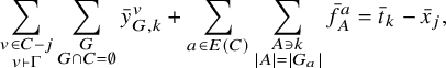 $$\begin{align*}\sum_{\substack{v \in C-j \\v \vdash \Gamma}} \sum_{\substack{ G\\ G \cap C = \emptyset}} \bar{y}_{G,k}^v + \sum_{a \in E(C)} \sum_{\substack{A \ni k\\\left| A \right| = \left| G_a \right|}} \bar{f}_A^{a} = \bar{t}_k - \bar{x}_j, \end{align*}$$
where G in the first double-sum is a connected component of
 $\Gamma - v$
,
$\Gamma - v$
,
 $G_{a}$
is the connected component of
$G_{a}$
is the connected component of
 $([n],E(\Gamma )\setminus \{(i,j)\})$
that is a subgraph of
$([n],E(\Gamma )\setminus \{(i,j)\})$
that is a subgraph of
 $G_{(i,j)}$
(i.e., does not contain j), and A in the second double-sum is a subset of
$G_{(i,j)}$
(i.e., does not contain j), and A in the second double-sum is a subset of
 $[n]$
. In particular,
$[n]$
. In particular,
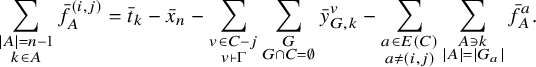 $$\begin{align*}\sum_{\substack{\left| A \right| = n-1 \\ k \in A}} \bar{f}_A^{(i,j)}= \bar{t}_k - \bar{x}_n- \sum_{\substack{v \in C-j \\v \vdash \Gamma}} \sum_{\substack{ G\\ G \cap C = \emptyset}} \bar{y}_{G,k}^v - \sum_{\substack{a \in E(C) \\ a\neq (i,j)}} \sum_{\substack{A \ni k\\\left| A \right|=\left| G_a \right| }} \bar{f}_A^{a}. \end{align*}$$
Now the right-hand side is in
 ${ \mathbb {C}\left \{\bar {\rho } \in \mathcal {F}_\Gamma \left | \bar {\rho } \neq \bar {f}_B^{(i,j)} \text { for any }B \subset [n] \right. \right \}}$
. Let
${ \mathbb {C}\left \{\bar {\rho } \in \mathcal {F}_\Gamma \left | \bar {\rho } \neq \bar {f}_B^{(i,j)} \text { for any }B \subset [n] \right. \right \}}$
. Let
 ${ \bar {\sigma }_k :=\sum _{\substack {\left | A \right | = n-1 \\ k \in A}} \bar {f}_A^{(i,j)},}$
so the above relation says
${ \bar {\sigma }_k :=\sum _{\substack {\left | A \right | = n-1 \\ k \in A}} \bar {f}_A^{(i,j)},}$
so the above relation says
 ${ \bar {\sigma }_k \in \\C\left \{\bar {\rho } \in \mathcal {F}_\Gamma \left | \bar {\rho } \neq \bar {f}_B^{(i,j)} \text { for any }B \subset [n] \right. \right \}}$
. For each
${ \bar {\sigma }_k \in \\C\left \{\bar {\rho } \in \mathcal {F}_\Gamma \left | \bar {\rho } \neq \bar {f}_B^{(i,j)} \text { for any }B \subset [n] \right. \right \}}$
. For each
 $p \in [n]$
, we have that
$p \in [n]$
, we have that
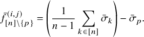 $$\begin{align*}\bar{f}_{[n] \setminus \{p\}}^{(i,j)} = \left(\frac{1}{n-1} \sum_{k \in [n]} \bar{\sigma}_k\right) - \bar{\sigma}_p. \end{align*}$$
Thus,
 ${ } \bar {f}_{[n] \setminus \{p\}}^{(i,j)} \in \mathbb {C}\left \{\bar {\rho } \in \mathcal {F}_\Gamma \left | \bar {\rho } \neq \bar {f}_B^{(i,j)} \text { for any }B \subset [n] \right. \right \}$
, and as all subsets of size
${ } \bar {f}_{[n] \setminus \{p\}}^{(i,j)} \in \mathbb {C}\left \{\bar {\rho } \in \mathcal {F}_\Gamma \left | \bar {\rho } \neq \bar {f}_B^{(i,j)} \text { for any }B \subset [n] \right. \right \}$
, and as all subsets of size
 $\left | A \right | = n-1$
take the form
$\left | A \right | = n-1$
take the form
 $A = [n] \setminus \{p\}$
, the claim follows.
$A = [n] \setminus \{p\}$
, the claim follows.
Example 5.8. If
 $\Gamma $
is the graph below where
$\Gamma $
is the graph below where
 $(12,13)$
is a leaf,
$(12,13)$
is a leaf,
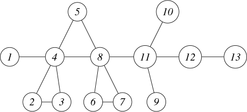
then Lemma 5.7 states that
 $\mathbb {C}\mathcal {F}_\Gamma $
is identical to
$\mathbb {C}\mathcal {F}_\Gamma $
is identical to
 ${ \mathbb {C}\left \{\bar {\rho } \in \mathcal {F}_\Gamma \left | \bar {\rho } \neq \bar {f}_B^{(12,13)} \text { for any }B \subset [n] \right. \right \}}$
.
${ \mathbb {C}\left \{\bar {\rho } \in \mathcal {F}_\Gamma \left | \bar {\rho } \neq \bar {f}_B^{(12,13)} \text { for any }B \subset [n] \right. \right \}}$
.
Since
 $(1,4)$
is also a leaf, we have that
$(1,4)$
is also a leaf, we have that
 $\mathbb {C}\mathcal {F}_\Gamma $
is equal to
$\mathbb {C}\mathcal {F}_\Gamma $
is equal to
 ${ \mathbb {C}\left \{\bar {\rho } \in \mathcal {F}_\Gamma \left | \bar {\rho } \neq \bar {f}_B^{(1,4)} \text { for any }B \subset [n] \right. \right \}}$
as well. Note we cannot remove the coset splines for
${ \mathbb {C}\left \{\bar {\rho } \in \mathcal {F}_\Gamma \left | \bar {\rho } \neq \bar {f}_B^{(1,4)} \text { for any }B \subset [n] \right. \right \}}$
as well. Note we cannot remove the coset splines for
 $(1,4)$
and
$(1,4)$
and
 $(12,13)$
from
$(12,13)$
from
 $\mathcal {F}_\Gamma $
at the same time and maintain the
$\mathcal {F}_\Gamma $
at the same time and maintain the
 $\mathbb {C}$
-span; we have to pick a particular leaf to remove and stick with it.
$\mathbb {C}$
-span; we have to pick a particular leaf to remove and stick with it.
6 Natural labels and cliqued graphs
In this section, we reduce the computation for arbitrary
 $\Gamma $
in two ways. First, we show that
$\Gamma $
in two ways. First, we show that
 $\Gamma $
may be replaced by a cliqued graph (defined below) without altering
$\Gamma $
may be replaced by a cliqued graph (defined below) without altering
 $\mathcal {M}_{\Gamma }^1$
. Second, we replace
$\mathcal {M}_{\Gamma }^1$
. Second, we replace
 $\Gamma $
with a particular representative of the isomorphism class we call naturally labeled. Subsection 6.2 gives three technical lemmas on splines that hold for these constructions.
$\Gamma $
with a particular representative of the isomorphism class we call naturally labeled. Subsection 6.2 gives three technical lemmas on splines that hold for these constructions.
First, if
 $\Gamma $
does not have a cut vertex, then it is
$\Gamma $
does not have a cut vertex, then it is
 $2$
-connected. Thus,
$2$
-connected. Thus,
 $\mathbf {ch}\left (\mathrm {L}_{\Gamma }\right )_1$
is trivial and
$\mathbf {ch}\left (\mathrm {L}_{\Gamma }\right )_1$
is trivial and
 $\mathbf {ch}\left (\mathrm {R}_{\Gamma }\right )_1$
is the first degree piece of the graded regular representation by Theorem 4.2 and Corollary 4.4. So we may assume that
$\mathbf {ch}\left (\mathrm {R}_{\Gamma }\right )_1$
is the first degree piece of the graded regular representation by Theorem 4.2 and Corollary 4.4. So we may assume that
 $\Gamma $
has a cut vertex; in particular, we may assume that
$\Gamma $
has a cut vertex; in particular, we may assume that
 $\Gamma $
has at least three vertices.
$\Gamma $
has at least three vertices.
A clique is a subgraph isomorphic to a complete graph. Let
 $\Gamma $
by any (connected) graph on
$\Gamma $
by any (connected) graph on
 $[n]$
. Call
$[n]$
. Call
 $\Gamma $
cliqued if two vertices are connected by an edge in
$\Gamma $
cliqued if two vertices are connected by an edge in
 $\Gamma $
whenever there exists two vertex-disjoint paths between them. Define
$\Gamma $
whenever there exists two vertex-disjoint paths between them. Define
 $$\begin{align*}\Gamma' = \left([n], E(\Gamma) \cup \{(i,j) \mid \; \text{exists two vertex-disjoint paths from }i\text{ to }j\text{ in }\Gamma\}\right).\end{align*}$$
Now
 $\Gamma '$
is cliqued, and we call
$\Gamma '$
is cliqued, and we call
 $\Gamma '$
the cliqued version of
$\Gamma '$
the cliqued version of
 $\Gamma $
. By Lemma 4.1, the first degree pieces of
$\Gamma $
. By Lemma 4.1, the first degree pieces of
 $\mathcal {M}_{\Gamma }$
and
$\mathcal {M}_{\Gamma }$
and
 $\mathcal {M}_{\Gamma '}$
are equal. Therefore, it suffices to consider cliqued graphs
$\mathcal {M}_{\Gamma '}$
are equal. Therefore, it suffices to consider cliqued graphs
 $\Gamma $
when proving results on the structure of
$\Gamma $
when proving results on the structure of
 $\mathcal {M}_{\Gamma }^1$
.
$\mathcal {M}_{\Gamma }^1$
.
Example 6.1. Below is an example of a graph
 $\Gamma $
and the cliqued graph
$\Gamma $
and the cliqued graph
 $\Gamma '$
such that
$\Gamma '$
such that
 $\mathcal {M}_{\Gamma }^1 = \mathcal {M}_{\Gamma '}^1$
:
$\mathcal {M}_{\Gamma }^1 = \mathcal {M}_{\Gamma '}^1$
:
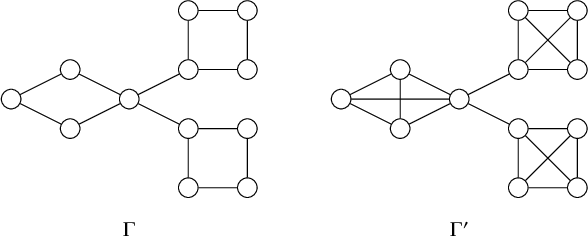
A 2-connected component of a graph
 $\Gamma $
is a subgraph of
$\Gamma $
is a subgraph of
 $\Gamma $
that is
$\Gamma $
that is
 $2$
-connected. A block is a maximal
$2$
-connected. A block is a maximal
 $2$
-connected component. In a cliqued graph, every block is a clique, and the process of cliquing a graph simply converts every block to a clique.
$2$
-connected component. In a cliqued graph, every block is a clique, and the process of cliquing a graph simply converts every block to a clique.
Definition 6.2. Let
 $\Gamma $
be a graph. The block-cut tree of
$\Gamma $
be a graph. The block-cut tree of
 $\Gamma $
is the tree with vertex set
$\Gamma $
is the tree with vertex set
 $$\begin{align*}\{v \mid v \vdash \Gamma\} \cup \{B \mid B\text{ is a block in } \Gamma\}\end{align*}$$
consisting of cut vertices and blocks in
 $\Gamma $
and edge set
$\Gamma $
and edge set
 $\{(v,B) \mid v \in B\}.$
Example 6.3. The graph on the left below is
 $\Gamma $
from Example 6.3 with the blocks and cut vertices labeled. The graph on the right below is the associated the block-cut tree. Note that the block-cut tree for the cliqued version
$\Gamma $
from Example 6.3 with the blocks and cut vertices labeled. The graph on the right below is the associated the block-cut tree. Note that the block-cut tree for the cliqued version
 $\Gamma '$
of
$\Gamma '$
of
 $\Gamma $
in Example 6.3 would be the same.
$\Gamma $
in Example 6.3 would be the same.
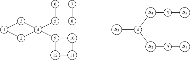
where
-
•
$B_1$
is the induced subgraph on vertices
$\{9,10,11,12\}$
-
•
$B_2$
is the induced subgraph on vertices
$\{4,9\}$
-
•
$B_3$
is the induced subgraph on vertices
$\{1,2,3,4\}$


-
•
$B_4$
is the induced subgraph on vertices
$\{4,5\}$
-
•
$B_5$
is the induced subgraph on vertices
$\{5,6,7,8\}$


It is easy to reason that the block-cut tree is indeed a tree by arguing that it cannot contain cycles. In a block-cut tree of a graph
 $\Gamma $
, every leaf is a block in
$\Gamma $
, every leaf is a block in
 $\Gamma $
and not a cut vertex, and paths in the block-cut tree alternate between cut-vertices and blocks. Since the block-cut tree ignores the internal structure of a
$\Gamma $
and not a cut vertex, and paths in the block-cut tree alternate between cut-vertices and blocks. Since the block-cut tree ignores the internal structure of a
 $2$
-connected component, the block-cut tree of a graph
$2$
-connected component, the block-cut tree of a graph
 $\Gamma $
and the block-cut tree of its cliqued version
$\Gamma $
and the block-cut tree of its cliqued version
 $\Gamma '$
are isomorphic as graphs.
$\Gamma '$
are isomorphic as graphs.
We now use the block-cut tree to construct a particular representative of the isomorphism class of
 $\Gamma $
. We will construct a bijection
$\Gamma $
. We will construct a bijection
 $\phi \colon [n] \to [n]$
to relabel the vertices of
$\phi \colon [n] \to [n]$
to relabel the vertices of
 $\Gamma $
.
$\Gamma $
.
Choose a cut vertex
 $v \vdash \Gamma $
such that v is adjacent to at most
$v \vdash \Gamma $
such that v is adjacent to at most
 $1$
block that is not a leaf in the block-cut tree of
$1$
block that is not a leaf in the block-cut tree of
 $\Gamma $
. One may obtain such a vertex v by (1) removing all leaves from the block-cut tree of
$\Gamma $
. One may obtain such a vertex v by (1) removing all leaves from the block-cut tree of
 $\Gamma $
(which must be blocks) and then (2) choosing a leaf from the tree that remains (which must be cut vertices). The vertices
$\Gamma $
(which must be blocks) and then (2) choosing a leaf from the tree that remains (which must be cut vertices). The vertices
 $5$
and
$5$
and
 $9$
satisfy this condition in Example 6.3.
$9$
satisfy this condition in Example 6.3.
Let B be the largest block that is also a leaf adjacent to v in the block-cut tree of
 $\Gamma $
. Since B is a leaf in the block-cut tree, there exists only a single cut vertex in B – namely,
$\Gamma $
. Since B is a leaf in the block-cut tree, there exists only a single cut vertex in B – namely,
 $v \in B$
. The following is the algorithm that produces
$v \in B$
. The following is the algorithm that produces
 $\phi \colon [n] \to [n]$
.
$\phi \colon [n] \to [n]$
.
-
1. Choose
$i \in B$
so that
$i \neq v$
. Define . Note n is adjacent to at most one cut vertex of
$\Gamma $
and is not itself a cut vertex of
$\Gamma $
. -
2. Define
$\phi $
on the remaining vertices in B as follows. Define
$\phi $
on
$B \setminus \{i,v\}$
so that
$d(j,i) < d(k,i)$
implies
$\phi (j)> \phi (k)$
for all
$j,k \in B \setminus \{i,v\}$
. Let -
3. Define
$\phi $
on the remaining vertices of
$\Gamma $
as follows. Let
$\phi $
be any bijection satisfying if
$j,k \in \Gamma \setminus V(B)$
, then
$d(j,i) < d(k,i)$
implies
$\phi (j)> \phi (k)$
.


Now that we have a bijection
 $\phi \colon [n] \to [n]$
, define a new graph
$\phi \colon [n] \to [n]$
, define a new graph ![]() . This graph is clearly isomorphic to
. This graph is clearly isomorphic to
 $\Gamma $
. We call the graph
$\Gamma $
. We call the graph
 $\Gamma "$
constructed in this manner naturally labeled.
$\Gamma "$
constructed in this manner naturally labeled.
Example 6.4. This example will construct a naturally labeled graph from the not-naturally labeled graph with
 $12$
vertices drawn below:
$12$
vertices drawn below:
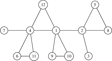
This has block-cut tree
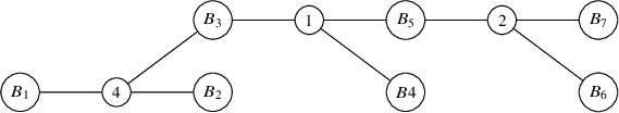
with blocks
-
•
$B_1$
on
$\{4,7\}$
-
•
$B_2$
on
$\{4,6,11\}$
-
•
$B_3$
on
$\{1,4,12\}$
-
•
$B_4$
on
$\{1,9,10\}$
-
•
$B_5$
on
$\{1,2\}$
-
•
$B_6$
on
$\{2,3\}$
-
•
$B_7$
on
$\{2,5,8\}$


To choose a vertex i such that
 $\phi (i) = 12$
, first we identify an appropriate cut vertex v. There are two cut vertices adjacent to only one non-leaf vertex in the block-cut tree,
$\phi (i) = 12$
, first we identify an appropriate cut vertex v. There are two cut vertices adjacent to only one non-leaf vertex in the block-cut tree,
 $2$
and
$2$
and
 $4$
. Let
$4$
. Let
 $v=2$
. The vertex
$v=2$
. The vertex
 $2$
is adjacent to blocks
$2$
is adjacent to blocks
 $B_6$
and
$B_6$
and
 $B_7$
in the block-cut tree. Since
$B_7$
in the block-cut tree. Since
 $B_7$
is bigger than
$B_7$
is bigger than
 $B_6$
, we know that either of
$B_6$
, we know that either of
 $i=5$
or
$i=5$
or
 $i=8$
will work. We choose
$i=8$
will work. We choose
 $i=8$
so
$i=8$
so
 $\phi (8) = 12$
, which concludes step (1).
$\phi (8) = 12$
, which concludes step (1).
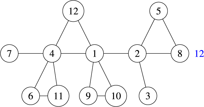
Now the block
 $B_7$
has three vertices, which leaves no choice for defining
$B_7$
has three vertices, which leaves no choice for defining
 $\phi $
on the remainder of
$\phi $
on the remainder of
 $B_7$
. So
$B_7$
. So
 $\phi (5) = 11$
and
$\phi (5) = 11$
and
 $\phi (4) = 10$
. This concludes step (2).
$\phi (4) = 10$
. This concludes step (2).
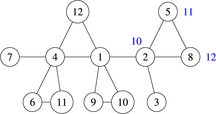
Finally, we define the rest of
 $\phi $
based on distance from the vertex
$\phi $
based on distance from the vertex
 $i=8$
and replace the old graph with the naturally labeled one. One possible natural label is the following:
$i=8$
and replace the old graph with the naturally labeled one. One possible natural label is the following:
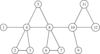
We note how many choices were made along the way. In particular, the isomorphism class of a graph
 $\Gamma $
may have many different naturally labeled members.
$\Gamma $
may have many different naturally labeled members.
We can use a natural label to more efficiently identify cut edges and connected components of a graph. The following definitions formalize this.
Definition 6.5. Let
 $\Gamma $
be a naturally labeled graph. If
$\Gamma $
be a naturally labeled graph. If
 $j \in \Gamma $
is a cut vertex, then
$j \in \Gamma $
is a cut vertex, then
 $i < j$
is j-dominant if i is the maximal value vertex in a connected component of
$i < j$
is j-dominant if i is the maximal value vertex in a connected component of
 $\Gamma - j$
that does not contain the vertex n. We call such an
$\Gamma - j$
that does not contain the vertex n. We call such an
 $(i,j)$
a dominant pair. A dominant pair
$(i,j)$
a dominant pair. A dominant pair
 $(i,j)$
is strongly dominant if
$(i,j)$
is strongly dominant if
 $(i,j)$
is a cut edge of
$(i,j)$
is a cut edge of
 $\Gamma $
, denoted
$\Gamma $
, denoted
 $(i,j) \gg \Gamma $
. Otherwise,
$(i,j) \gg \Gamma $
. Otherwise,
 $(i,j)$
is weakly dominant, denoted
$(i,j)$
is weakly dominant, denoted
 $(i,j)>\Gamma $
.
$(i,j)>\Gamma $
.
There are four things to note about dominant pairs.
-
1. Even if
$(n-1,n)$
is a cut edge,
$(n-1,n)$
is never a strongly dominant pair since n is not a cut vertex by the definition of a natural label. However, every other cut edge in a naturally labeled graph
$\Gamma $
is a strongly dominant pair, since the higher-labeled vertex in the cut edge must be a cut vertex. -
2. If
$j \vdash \Gamma $
, then all vertices larger than j must be concentrated in one connected component of
$\Gamma - j$
. If k is in a connected component of
$\Gamma - j$
that does not contain the vertex n, then any path from k to n must pass through j, and so
$d(k,n)> d(j,n)$
, and thus,
$k<j$
by the definition of a natural label. In particular, the only connected component of
$\Gamma - j$
whose maximal vertex is greater than j is the one that contains n, so each connected component of
$\Gamma - j$
that does not contain n contains precisely one j-dominant vertex. -
3. Since a natural label is constructed by distance from n, for each cut vertex j, the maximal-labeled vertices in a connected component of
$\Gamma - j$
that does not contain n must be adjacent to j. In particular, dominant pairs are also edges. -
4. The lower vertex in the dominant pair uniquely determines the pair. In particular, if for contradiction we assume
$(i,j)$
and
$(i,k)$
are both dominant pairs, then i and k are in the same connected component of
$\Gamma - j$
, and
$i<k$
, and so
$(i,j)$
is not a dominant pair.


Definition 6.6. Let
 $\Gamma $
be naturally labeled and fix
$\Gamma $
be naturally labeled and fix
 $j \in \Gamma $
. Let
$j \in \Gamma $
. Let ![]() , and
, and ![]() . If j is not a cut vertex, then
. If j is not a cut vertex, then
 $\mathfrak {C}_\Gamma (j) = \emptyset $
and
$\mathfrak {C}_\Gamma (j) = \emptyset $
and
 $\mathfrak {c}_\Gamma (j) = 0$
. If j is a cut vertex of
$\mathfrak {c}_\Gamma (j) = 0$
. If j is a cut vertex of
 $\Gamma $
, then the cut decomposition of
$\Gamma $
, then the cut decomposition of
 $\Gamma -j$
is
$\Gamma -j$
is
where
 $\Gamma _i^j$
the connected component of
$\Gamma _i^j$
the connected component of
 $\Gamma - j$
such that
$\Gamma - j$
such that
 $i \in \Gamma _i^j$
and
$i \in \Gamma _i^j$
and
 $\Gamma _0^j$
denotes the single connected component of
$\Gamma _0^j$
denotes the single connected component of
 $\Gamma - j$
where
$\Gamma - j$
where
 $n \in \Gamma _0^j$
.
$n \in \Gamma _0^j$
.
So if
 $j \vdash \Gamma $
is a cut vertex of
$j \vdash \Gamma $
is a cut vertex of
 $\Gamma $
and
$\Gamma $
and
 $k \in [n]$
such that
$k \in [n]$
such that
 $k> j$
, then
$k> j$
, then
 $k \in \Gamma _0^j$
. When
$k \in \Gamma _0^j$
. When
 $\Gamma $
is obvious from context, we write
$\Gamma $
is obvious from context, we write
 $\mathfrak {C}(j)$
and
$\mathfrak {C}(j)$
and
 $\mathfrak {c}(j)$
without the subscripts.
$\mathfrak {c}(j)$
without the subscripts.
Remark 6.7. If
 $(i,j)$
is a cut edge and j is a cut vertex, then
$(i,j)$
is a cut edge and j is a cut vertex, then
 $\Gamma _i^j$
as in the cut decomposition of
$\Gamma _i^j$
as in the cut decomposition of
 $\Gamma - j$
is one of the two connected components of
$\Gamma - j$
is one of the two connected components of
 $([n],E(\Gamma ) \setminus \{(i,j)\})$
. In particular,
$([n],E(\Gamma ) \setminus \{(i,j)\})$
. In particular,
 $\Gamma _i^j$
is one of the two valid choices for
$\Gamma _i^j$
is one of the two valid choices for
 $G_s$
when defining
$G_s$
when defining
 $\bar {f}_A^{(i,j)}$
at the beginning of Section 5. From now on, even if
$\bar {f}_A^{(i,j)}$
at the beginning of Section 5. From now on, even if
 $\Gamma $
is not naturally labeled and even if the cut edge is
$\Gamma $
is not naturally labeled and even if the cut edge is
 $(i,j) = (n-1,n)$
, we will choose
$(i,j) = (n-1,n)$
, we will choose
 $G_s$
to be the connected component of
$G_s$
to be the connected component of
 $(V(\Gamma ),E(\Gamma )-(i,j))$
that contains
$(V(\Gamma ),E(\Gamma )-(i,j))$
that contains
 $i < j$
, so that the notation always agrees with Definition 6.6.
$i < j$
, so that the notation always agrees with Definition 6.6.
Example 6.8. The following is the cliqued and naturally labeled graph
 $\Gamma $
from Example 6.4. We have labeled the strongly dominant pairs in double lines and the weakly dominant pairs in dashed lines:
$\Gamma $
from Example 6.4. We have labeled the strongly dominant pairs in double lines and the weakly dominant pairs in dashed lines:
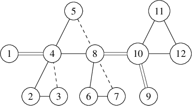
The cut vertices are
 $\{4,8,10\}$
, and
$\{4,8,10\}$
, and
 $\mathfrak {c}_{\Gamma }(10) = \mathfrak {c}_{\Gamma }(8) =\mathfrak {c}_{\Gamma }(4) = 2$
. The graph
$\mathfrak {c}_{\Gamma }(10) = \mathfrak {c}_{\Gamma }(8) =\mathfrak {c}_{\Gamma }(4) = 2$
. The graph
 $\Gamma - 8$
is displayed below, with the cut decomposition labeled:
$\Gamma - 8$
is displayed below, with the cut decomposition labeled:
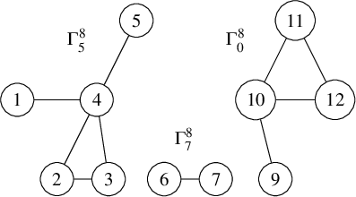
Lemma 6.9 below summarizes some properties of a cliqued and naturally labeled graph.
Lemma 6.9. If
 $\Gamma $
is cliqued and naturally labeled, then
$\Gamma $
is cliqued and naturally labeled, then
-
(A) if
$i,j \in \mathrm {N}(n)$
are both adjacent to the vertex n in
$\Gamma $
, then
$(i,j) \in E(\Gamma )$
, -
(B) if
$n-1 \vdash \Gamma $
is a cut vertex of
$\Gamma $
, then at most one of the connected components
$\Gamma _i^{n-1}$
for
$i \in \mathfrak {C}_{\Gamma }(n-1)$
in the cut decomposition of
$\Gamma - (n-1)$
is not a single vertex, -
(C) If
$r,k \in \Gamma _i^j \cap \mathrm {N}(j)$
are vertices both adjacent to
$j\vdash \Gamma $
and in the same connected component of
$\Gamma - j$
, then
$(r,k) \in E(\Gamma )$
.


Proof. Let
 $B_0$
be the block in
$B_0$
be the block in
 $\Gamma $
that contains n.
$\Gamma $
that contains n.
(1) If
 $i,j \in \mathrm {N}(n)$
, then
$i,j \in \mathrm {N}(n)$
, then
 $i,j \in B_0$
. Since
$i,j \in B_0$
. Since
 $\Gamma $
is cliqued,
$\Gamma $
is cliqued,
 $B_0$
must be a clique and so
$B_0$
must be a clique and so
 $(i,j) \in E(\Gamma )$
.
$(i,j) \in E(\Gamma )$
.
(2) The vertex
 $n-1$
is a cut vertex of
$n-1$
is a cut vertex of
 $\Gamma $
if and only if n is a leaf, and
$\Gamma $
if and only if n is a leaf, and
 $B_0$
is size
$B_0$
is size
 $2$
. Since
$2$
. Since
 $\Gamma $
is naturally labeled,
$\Gamma $
is naturally labeled,
 $n-1$
is adjacent to at most one block that is not a leaf in the block-cut tree of
$n-1$
is adjacent to at most one block that is not a leaf in the block-cut tree of
 $\Gamma $
, and
$\Gamma $
, and
 $B_0$
is of maximal size among those leaves in the block-cut tree. Thus, the blocks adjacent to
$B_0$
is of maximal size among those leaves in the block-cut tree. Thus, the blocks adjacent to
 $n-1$
in the block-cut tree of
$n-1$
in the block-cut tree of
 $\Gamma $
are either not a leaf in the block-cut tree (of which there can only be one) or a leaf in the block-cut tree and size no greater than
$\Gamma $
are either not a leaf in the block-cut tree (of which there can only be one) or a leaf in the block-cut tree and size no greater than
 $2$
.
$2$
.
(3) There exists a path
 $(r,j,k)$
in
$(r,j,k)$
in
 $\Gamma $
, and another path from r to k in
$\Gamma $
, and another path from r to k in
 $\Gamma _i^j$
, which does not contain the vertex j. Since
$\Gamma _i^j$
, which does not contain the vertex j. Since
 $\Gamma $
is cliqued and we know there are two vertex-disjoint paths from r to k in
$\Gamma $
is cliqued and we know there are two vertex-disjoint paths from r to k in
 $\Gamma $
, it follows that
$\Gamma $
, it follows that
 $(r,k) \in E(\Gamma )$
.
$(r,k) \in E(\Gamma )$
.
We use Lemma 6.9 to categorize cliqued and naturally labeled graphs in to three types, based on the structure of
 $\Gamma $
near the vertex n.
$\Gamma $
near the vertex n.
Lemma 6.10. If
 $\Gamma $
is cliqued and naturally labeled, then it falls in to one of the following three types:
$\Gamma $
is cliqued and naturally labeled, then it falls in to one of the following three types:
-
(A) The edge
$(n-1,n)$
is a cut edge of
$\Gamma $
, and at most one component of
$\Gamma - (n-1)$
is not an isolated vertex. -
(B) The vertex
$n-2$
is a cut vertex, and the vertices
$\{n-2,n-1,n\}$
form a block in
$\Gamma $
. -
(C) None of the vertices
$\{n,n-1,n-2\}$
are cut vertices, and
$\{n-2,n-1,n\}$
form a clique in
$\Gamma $
.


Proof. Categorize
 $\Gamma $
by the size of the neighborhood
$\Gamma $
by the size of the neighborhood
 $\mathrm {N}(n)$
. For every
$\mathrm {N}(n)$
. For every
 $\Gamma $
, exactly one of the following is true:
$\Gamma $
, exactly one of the following is true:
 $\left | \mathrm {N}{(n)} \right | = 1$
,
$\left | \mathrm {N}{(n)} \right | = 1$
,
 $\left | \mathrm {N}{(n)} \right | = 2$
or
$\left | \mathrm {N}{(n)} \right | = 2$
or
 $\left | \mathrm {N}(n) \right |> 2$
. Note that, since every block is a clique and n is not a cut vertex, the block B containing n has vertices
$\left | \mathrm {N}(n) \right |> 2$
. Note that, since every block is a clique and n is not a cut vertex, the block B containing n has vertices
 $N(n) \cup \{n\}$
.
$N(n) \cup \{n\}$
.
If
 $\left | \mathrm {N}{(n)} \right | = 1$
, then
$\left | \mathrm {N}{(n)} \right | = 1$
, then
 $n-1$
is a cut vertex, and
$n-1$
is a cut vertex, and
 $\Gamma $
is type A. The rest of the claim for type A is Lemma 6.9(2).
$\Gamma $
is type A. The rest of the claim for type A is Lemma 6.9(2).
Suppose
 $\left | \mathrm {N}{(n)} \right | = 2$
. Since
$\left | \mathrm {N}{(n)} \right | = 2$
. Since
 $\Gamma $
is naturally labeled,
$\Gamma $
is naturally labeled,
 $n-2$
must be a cut vertex. We also have
$n-2$
must be a cut vertex. We also have
 $(n-2,n-1) \in E(\Gamma )$
by Lemma 6.9(1).
$(n-2,n-1) \in E(\Gamma )$
by Lemma 6.9(1).
Finally, suppose
 $\left | \mathrm {N}{(n)} \right |> 2$
. Since
$\left | \mathrm {N}{(n)} \right |> 2$
. Since
 $\Gamma $
is naturally labeled, none of
$\Gamma $
is naturally labeled, none of
 $\{n-2,n-1,n\}$
is a cut vertex. Once again,
$\{n-2,n-1,n\}$
is a cut vertex. Once again,
 $(n-2,n-1) \in E(\Gamma )$
by Lemma 6.9(1).
$(n-2,n-1) \in E(\Gamma )$
by Lemma 6.9(1).
Visually, Lemma 6.10 says that if
 $\Gamma $
is cliqued and naturally labeled, then
$\Gamma $
is cliqued and naturally labeled, then
 $\Gamma $
can be represented diagrammatically in one of the following three ways:
$\Gamma $
can be represented diagrammatically in one of the following three ways:
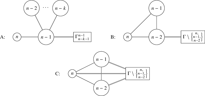
In the diagram for type A above,
 $\mathfrak {c}_{\Gamma }(n-1) = k$
. We remark that in type B, the induced subgraph
$\mathfrak {c}_{\Gamma }(n-1) = k$
. We remark that in type B, the induced subgraph
 $\Gamma \setminus \{n-2,n-2,n\}$
may be disconnected (such as it would be for the graph in Example 6.8). However, in type C, the vertex
$\Gamma \setminus \{n-2,n-2,n\}$
may be disconnected (such as it would be for the graph in Example 6.8). However, in type C, the vertex
 $n-3$
must be in the same block as n,
$n-3$
must be in the same block as n,
 $n-1$
and
$n-1$
and
 $n-2$
, so the induced subgraph
$n-2$
, so the induced subgraph
 $\Gamma \setminus \{n-2,n-1,n\}$
is actually connected.
$\Gamma \setminus \{n-2,n-1,n\}$
is actually connected.
Example 6.11. The graph
 $\Gamma $
from Example 6.8 is type B. The following is a naturally labeled type A graph:
$\Gamma $
from Example 6.8 is type B. The following is a naturally labeled type A graph:
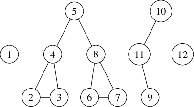
A different natural label on the same graph, such as the one below, can have a different classification. The following naturally labeled graph is in the same isomorphism class as the previous, but is type B:
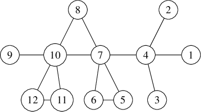
6.1 The spanning set revisited
A natural labeling provides a more convenient indexing for the splines in
 $\mathcal {Y}_\Gamma $
and
$\mathcal {Y}_\Gamma $
and
 $\mathcal {C}_\Gamma $
, using the cut decomposition from Definition 6.6. In particular, we write
$\mathcal {C}_\Gamma $
, using the cut decomposition from Definition 6.6. In particular, we write
so that
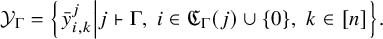 $$\begin{align*}\mathcal{Y}_\Gamma = \left\{\left.\bar{y}_{i,k}^j \right| j \vdash \Gamma,\; i \in \mathfrak{C}_{\Gamma}(j)\cup\{0\},\; k \in [n]\right\}.\end{align*}$$
Additionally, while the notation for individual splines
 $\bar {f}_A^s \in \mathcal {C}_\Gamma $
does not change, we note that, as stated in Remark 6.7, we choose
$\bar {f}_A^s \in \mathcal {C}_\Gamma $
does not change, we note that, as stated in Remark 6.7, we choose
 $G_{s}$
for
$G_{s}$
for
 $s=(i<j)$
to be equal to
$s=(i<j)$
to be equal to
 $\Gamma _i^j$
.
$\Gamma _i^j$
.
We collect the important naturally-labeled versions of Lemmas 5.6, 5.5 and 5.7 below in Proposition 6.12.
Proposition 6.12. Let
 $\Gamma $
be naturally labeled, and let
$\Gamma $
be naturally labeled, and let

Then the following hold:
-
1. If
$(i,j) \gg \Gamma $
, then
$\bar {y}_{i,k}^j \in \mathbb {C} \mathcal {B}_\Gamma $
for all
$k \in [n]$
. -
2. If
$j \vdash \Gamma $
, then
$\bar {y}_{0,k}^j \in \mathbb {C} \mathcal {B}_\Gamma $
for all
$k \in [n]$
. -
3. If
$(n-1,n)$
is a cut edge of
$\Gamma $
, then
$\bar {f}_{A}^{(n-1,n)} \in \mathbb {C}\mathcal {B}_\Gamma $
for all
$A \subset [n]$
where
$\left | A \right | = n-1$
.


In particular,
 $\mathbb {C}\mathcal {B}_\Gamma = \mathbb {C}\mathcal {F}_\Gamma $
.
$\mathbb {C}\mathcal {B}_\Gamma = \mathbb {C}\mathcal {F}_\Gamma $
.

6.2 Technical lemmas
This subsection contains three lemmas that are used within the proof of Theorem 7.2.
Let
![]() be a left coset of
be a left coset of
 $S_{n-1}$
in
$S_{n-1}$
in
 $S_n$
. The first Lemma 6.13 establishes what values a linear spline
$S_n$
. The first Lemma 6.13 establishes what values a linear spline
 $\bar {\rho }$
may take on
$\bar {\rho }$
may take on
 $S_n^{n-1}$
if
$S_n^{n-1}$
if
 $\bar {\rho }$
is not supported on
$\bar {\rho }$
is not supported on
 $S_n^n = S_{n-1}$
.
$S_n^n = S_{n-1}$
.
Lemma 6.13. Let
 $\Gamma $
be naturally labeled, and
$\Gamma $
be naturally labeled, and
 $\bar {\rho } \in \mathcal {M}_{\Gamma }^1$
, where
$\bar {\rho } \in \mathcal {M}_{\Gamma }^1$
, where
 $\bar {\rho } \equiv 0$
on
$\bar {\rho } \equiv 0$
on
 $S_n^n$
. If
$S_n^n$
. If
 $w,v \in S_n^{n-1}$
, then
$w,v \in S_n^{n-1}$
, then
 $\bar {\rho }(w) = c_w\left (t_n-t_{w(n)}\right )$
and
$\bar {\rho }(w) = c_w\left (t_n-t_{w(n)}\right )$
and
 $\bar {\rho }(v) = c_v\left (t_n-t_{v(n)}\right )$
for some
$\bar {\rho }(v) = c_v\left (t_n-t_{v(n)}\right )$
for some
 $c_w,c_v \in \mathbb {C}$
. Furthermore, if
$c_w,c_v \in \mathbb {C}$
. Furthermore, if
 $w(n) = v(n)$
, or
$w(n) = v(n)$
, or
 $\Gamma $
is type
$\Gamma $
is type
 $B/C$
, then
$B/C$
, then
 $c_w=c_v$
.
$c_w=c_v$
.
Proof. First, since
 $\Gamma $
is naturally labeled, it follows that
$\Gamma $
is naturally labeled, it follows that
 $(n-1,n) \in E(\Gamma )$
. We will show the first part of the claim for
$(n-1,n) \in E(\Gamma )$
. We will show the first part of the claim for
 $w \in S_n^{n-1}$
, and the same will hold for
$w \in S_n^{n-1}$
, and the same will hold for
 $v \in S_n^{n-1}$
. If
$v \in S_n^{n-1}$
. If
 $w \in S_n^{n-1}$
, then
$w \in S_n^{n-1}$
, then
 $w(n-1,n) \in S_n^n$
, and
$w(n-1,n) \in S_n^n$
, and
 $\mathcal {L}(w,w(n-1,n)) = \left \langle t_{w(n-1)} - t_{w(n)}\right \rangle = \left \langle t_n - t_{w(n)} \right \rangle $
. Since
$\mathcal {L}(w,w(n-1,n)) = \left \langle t_{w(n-1)} - t_{w(n)}\right \rangle = \left \langle t_n - t_{w(n)} \right \rangle $
. Since
 $\bar {\rho }$
is linear and
$\bar {\rho }$
is linear and
 $\bar {\rho }(w(n-1,n)) = 0$
, the first part of the claim follows.
$\bar {\rho }(w(n-1,n)) = 0$
, the first part of the claim follows.
Now we prove the second part of the claim. First, we assume
 $w(n) = v(n)$
. Two permutations
$w(n) = v(n)$
. Two permutations
 $w,v \in S_n^{n-1}$
have the property
$w,v \in S_n^{n-1}$
have the property
 $w(n) = v(n)$
if and only if
$w(n) = v(n)$
if and only if
 $v \in wS_{n-2}$
. The claim will follow if
$v \in wS_{n-2}$
. The claim will follow if
 $c_w=c_v$
for
$c_w=c_v$
for
 $v = w(r,s)$
whenever
$v = w(r,s)$
whenever
 $(r,s) \in S_{n-2}$
. Let
$(r,s) \in S_{n-2}$
. Let
 $\{r,s\} \subset [n-2]$
. As
$\{r,s\} \subset [n-2]$
. As
 $\Gamma $
is naturally labeled and so n is not a cut vertex of
$\Gamma $
is naturally labeled and so n is not a cut vertex of
 $\Gamma $
, there exists a simple path
$\Gamma $
, there exists a simple path
 $(r_0,r_1,...,r_m)$
in
$(r_0,r_1,...,r_m)$
in
 $\Gamma $
from
$\Gamma $
from
 $r=r_0$
to
$r=r_0$
to
 $s=r_m$
that does not contain n, and by Lemma 3.3,
$s=r_m$
that does not contain n, and by Lemma 3.3,
 $$\begin{align*}\bar{\rho}(w) - \bar{\rho}(w(r,s)) \in \left\langle t_{w(r_i)} - t_{w(r_{i-1})} \mid i \in [m]\right\rangle.\end{align*}$$
In particular,
 $$\begin{align*}(c_w-c_{w(r,s)})t_n - (c_w - c_{w(r,s)}) t_{w(n)} \in \left\langle t_{w(r_i)} - t_{w(r_{i-1})} \mid i \in [m]\right\rangle.\end{align*}$$
The monomial
 $t_{w(n)}$
does not appear in
$t_{w(n)}$
does not appear in
 $\{t_{w(r_i)} - t_{w(r_{i-1})} \mid i \in [m]\}$
, and thus,
$\{t_{w(r_i)} - t_{w(r_{i-1})} \mid i \in [m]\}$
, and thus,
 $c_{w} = c_{w(r,s)}$
. Since the transpositions
$c_{w} = c_{w(r,s)}$
. Since the transpositions
 $(r,s)$
generate
$(r,s)$
generate
 $S_{n-2}$
, the claim follows.
$S_{n-2}$
, the claim follows.
Now we prove the claim if
 $\Gamma $
is type
$\Gamma $
is type
 $B/C$
. If
$B/C$
. If
 $\Gamma $
is type B or type C, then
$\Gamma $
is type B or type C, then
 $\Gamma -(n-1)$
is connected. It suffices to prove
$\Gamma -(n-1)$
is connected. It suffices to prove
 $c_w = c_{w(r,s)}$
for
$c_w = c_{w(r,s)}$
for
 $n-1 \notin \{r,s\}$
. Since
$n-1 \notin \{r,s\}$
. Since
 $\Gamma - (n-1)$
is connected, there exists a path
$\Gamma - (n-1)$
is connected, there exists a path
 $(r_0,...,r_m)$
from
$(r_0,...,r_m)$
from
 $r=r_0$
to
$r=r_0$
to
 $s=r_m$
in
$s=r_m$
in
 $\Gamma $
that does not visit the vertex
$\Gamma $
that does not visit the vertex
 $n-1$
. So
$n-1$
. So
 $$\begin{align*}(c_w-c_{w(r,s)})t_n - c_wt_{w(n)} - c_{w(r,s)} t_{w(r,s)(n)} \in \left\langle t_{w(r_i)} - t_{w(r_{i-1})} \mid i \in [m]\right\rangle.\end{align*}$$
Now
 $t_n = t_{w(n-1)}$
never appears in
$t_n = t_{w(n-1)}$
never appears in
 $\left \{ t_{w(r_i)} - t_{w(r_{i-1})} \mid i \in [m]\right \}$
, and thus,
$\left \{ t_{w(r_i)} - t_{w(r_{i-1})} \mid i \in [m]\right \}$
, and thus,
 $c_w=c_v$
.
$c_w=c_v$
.
The second two lemmas assume that
 $(i,j)$
is a dominant pair in
$(i,j)$
is a dominant pair in
 $\Gamma $
and establish what values a linear spline
$\Gamma $
and establish what values a linear spline
 $\bar {\rho }$
may take on
$\bar {\rho }$
may take on
 $S_n^i$
if
$S_n^i$
if
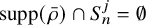 $\mathrm {supp}(\bar {\rho }) \cap S_n^j = \emptyset $
. Lemma 6.14 below assumes
$\mathrm {supp}(\bar {\rho }) \cap S_n^j = \emptyset $
. Lemma 6.14 below assumes
 $(i,j)$
is strongly dominant and relates
$(i,j)$
is strongly dominant and relates
 $\bar {\rho }(w)$
to
$\bar {\rho }(w)$
to
 $\bar {\rho }(v)$
if w and v are in the same coset
$\bar {\rho }(v)$
if w and v are in the same coset
 $S_n^i$
and they are also in the same coset of the reflection subgroup generated by the transpositions
$S_n^i$
and they are also in the same coset of the reflection subgroup generated by the transpositions
 $E(\Gamma ) \setminus \{(i,j)\}$
.
$E(\Gamma ) \setminus \{(i,j)\}$
.
Lemma 6.14. Let
 $\Gamma $
be cliqued and naturally labeled, and say
$\Gamma $
be cliqued and naturally labeled, and say
 $(i,j) \gg \Gamma $
. Let
$(i,j) \gg \Gamma $
. Let
 $\bar {\rho } \in \mathcal {M}_{\Gamma }^1$
, where
$\bar {\rho } \in \mathcal {M}_{\Gamma }^1$
, where
 $\bar {\rho } \equiv 0$
on
$\bar {\rho } \equiv 0$
on
 $S_n^j$
. If
$S_n^j$
. If
 $w,v \in S_n^{i}$
, then
$w,v \in S_n^{i}$
, then
 $\bar {\rho }(w) = c_w\left (t_n-t_{w(j)}\right )$
and
$\bar {\rho }(w) = c_w\left (t_n-t_{w(j)}\right )$
and
 $\bar {\rho }(v) = c_v\left (t_n-t_{v(j)}\right )$
for some
$\bar {\rho }(v) = c_v\left (t_n-t_{v(j)}\right )$
for some
 $c_w,c_v \in \mathbb {C}$
. Furthermore, if
$c_w,c_v \in \mathbb {C}$
. Furthermore, if
 $v \in w\langle E(\Gamma )\setminus (i,j)\rangle $
, then
$v \in w\langle E(\Gamma )\setminus (i,j)\rangle $
, then
 $c_w=c_v$
.
$c_w=c_v$
.
Proof. First, since
 $\Gamma $
is naturally labeled, it follows that
$\Gamma $
is naturally labeled, it follows that
 $(i,j) \in E(\Gamma )$
. We will show the first part of the claim for
$(i,j) \in E(\Gamma )$
. We will show the first part of the claim for
 $w \in S_n^i$
, and the same will hold for
$w \in S_n^i$
, and the same will hold for
 $v \in S_n^i$
. If
$v \in S_n^i$
. If
 $w \in S_n^i$
, then
$w \in S_n^i$
, then
 $w(i,j) \in S_n^j$
, and
$w(i,j) \in S_n^j$
, and
 $\mathcal {L}(w,w(i,j)) = \left \langle t_{w(i)} - t_{w(j)}\right \rangle = \left \langle t_n - t_{w(j)} \right \rangle $
. Since
$\mathcal {L}(w,w(i,j)) = \left \langle t_{w(i)} - t_{w(j)}\right \rangle = \left \langle t_n - t_{w(j)} \right \rangle $
. Since
 $\bar {\rho }$
is linear and
$\bar {\rho }$
is linear and
 $\bar {\rho }(w(i,j)) = 0$
, the first part of the claim follows from the definition of a spline on
$\bar {\rho }(w(i,j)) = 0$
, the first part of the claim follows from the definition of a spline on
 $\mathcal {G}_\Gamma $
.
$\mathcal {G}_\Gamma $
.
The reflection subgroup
 $\left \langle E(\Gamma ) \setminus \{(i,j)\}\right \rangle $
is also generated by the transpositions
$\left \langle E(\Gamma ) \setminus \{(i,j)\}\right \rangle $
is also generated by the transpositions
 $\{(r,s) \mid \{r,s\} \subset V(\Gamma _i^j)\} \cup \{(p,q) \mid \{p,q\} \subset [n] \setminus V(\Gamma _i^j)\}$
, as this set contains
$\{(r,s) \mid \{r,s\} \subset V(\Gamma _i^j)\} \cup \{(p,q) \mid \{p,q\} \subset [n] \setminus V(\Gamma _i^j)\}$
, as this set contains
 $E(\Gamma ) \setminus \{i,j\}$
. We will show that, for those generating transpositions,
$E(\Gamma ) \setminus \{i,j\}$
. We will show that, for those generating transpositions,
 $c_w = c_{w(r,s)}$
and
$c_w = c_{w(r,s)}$
and
 $c_w = c_{w(p,q)}$
.
$c_w = c_{w(p,q)}$
.
First, we show
 $c_w = c_{w(r,s)}$
for
$c_w = c_{w(r,s)}$
for
 $\{r,s\} \subset V(\Gamma _i^j)$
. Let
$\{r,s\} \subset V(\Gamma _i^j)$
. Let
 $(r_0,...,r_m)$
be a path in
$(r_0,...,r_m)$
be a path in
 $\Gamma _i^j$
from
$\Gamma _i^j$
from
 $r=r_0$
to
$r=r_0$
to
 $r_m=s$
. Then by Lemma 3.3,
$r_m=s$
. Then by Lemma 3.3,
 $$\begin{align*}\bar{\rho}(w) - \bar{\rho}(w(r,s)) \in \left\langle t_{w(r_k)} - t_{w(r_{k-1})} \mid k \in [m]\right\rangle.\end{align*}$$
In particular,
 $$\begin{align*}(c_w-c_{w(r,s)})t_n - (c_w - c_{w(r,s)}) t_{w(j)} \in \left\langle t_{w(r_k)} - t_{w(r_{k-1})} \mid k \in [m]\right\rangle.\end{align*}$$
Since j is not in the path
 $(r_0,...,r_m)$
, the monomial
$(r_0,...,r_m)$
, the monomial
 $t_{w(j)}$
does not appear in
$t_{w(j)}$
does not appear in
 $\{t_{w(r_k)} - t_{w(r_{k-1})} \mid k \in [m]\}$
, and thus,
$\{t_{w(r_k)} - t_{w(r_{k-1})} \mid k \in [m]\}$
, and thus,
 $c_{w} = c_{w(r,s)}$
.
$c_{w} = c_{w(r,s)}$
.
Now let
 $\{p,q\} \subset [n] \setminus V(\Gamma _i^j)$
. Since
$\{p,q\} \subset [n] \setminus V(\Gamma _i^j)$
. Since
 $(i,j)$
is a cut edge, the induced subgraph of
$(i,j)$
is a cut edge, the induced subgraph of
 $\Gamma $
with vertex set
$\Gamma $
with vertex set
 $[n] \setminus V(\Gamma _i^j)$
is connected. Let
$[n] \setminus V(\Gamma _i^j)$
is connected. Let
 $(p_0,...,p_m)$
be a path from
$(p_0,...,p_m)$
be a path from
 $p = p_0$
to
$p = p_0$
to
 $q=p_m$
in
$q=p_m$
in
 $\Gamma $
that does not contain i. By Lemma 3.3,
$\Gamma $
that does not contain i. By Lemma 3.3,
 $$\begin{align*}\bar{\rho}(w) - \bar{\rho}(w(p,q)) \in \left\langle t_{w(p_k)} - t_{w(p_{k-1})} \mid k \in [m]\right\rangle.\end{align*}$$
In particular,
 $$\begin{align*}(c_w-c_{w(p,q)})t_n - c_wt_{w(j)} + c_{w(p,q)} t_{w(p,q)(j)} \in \left\langle t_{w(p_k)} - t_{w(p_{k-1})} \mid k \in [m]\right\rangle.\end{align*}$$
Since i is not in the path
 $(p_0,...,p_m)$
, the monomial
$(p_0,...,p_m)$
, the monomial
 $t_n = t_{w(i)}$
does not appear in
$t_n = t_{w(i)}$
does not appear in
 $\{t_{w(p_k)} - t_{w(p_{k-1})} \mid k \in [m]\}$
, and thus,
$\{t_{w(p_k)} - t_{w(p_{k-1})} \mid k \in [m]\}$
, and thus,
 $c_w=c_{w(p,q)}$
.
$c_w=c_{w(p,q)}$
.
Since the reflection subgroup
 $\langle E(\Gamma )\setminus (i,j)\rangle $
is generated by
$\langle E(\Gamma )\setminus (i,j)\rangle $
is generated by
 $\{(r,s) \mid \{r,s\} \subset \Gamma _i^j\} \cup \{(p,q) \mid \{p,q\} \in [n]\setminus \Gamma _i^j\}$
, the claim follows.
$\{(r,s) \mid \{r,s\} \subset \Gamma _i^j\} \cup \{(p,q) \mid \{p,q\} \in [n]\setminus \Gamma _i^j\}$
, the claim follows.
Lemma 6.15 below assumes that
 $(i,j)$
is weakly dominant and then relates
$(i,j)$
is weakly dominant and then relates
 $\bar {\rho }(w)$
and
$\bar {\rho }(w)$
and
 $\bar {\rho }(v)$
if w and v are in the same coset
$\bar {\rho }(v)$
if w and v are in the same coset
 $S_n^i$
.
$S_n^i$
.
Lemma 6.15. Let
 $\Gamma $
be cliqued and naturally labeled, and say
$\Gamma $
be cliqued and naturally labeled, and say
 $(i,j)>\Gamma $
. Let
$(i,j)>\Gamma $
. Let
 $\bar {\rho } \in \mathcal {M}_{\Gamma }^1$
, where
$\bar {\rho } \in \mathcal {M}_{\Gamma }^1$
, where
 $\bar {\rho } \equiv 0$
on
$\bar {\rho } \equiv 0$
on
 $S_n^j$
. If
$S_n^j$
. If
 $w,v \in S_n^{i}$
, then
$w,v \in S_n^{i}$
, then
 $\bar {\rho }(w) = c_w\left (t_n-t_{w(j)}\right )$
and
$\bar {\rho }(w) = c_w\left (t_n-t_{w(j)}\right )$
and
 $\bar {\rho }(v) = c_v\left (t_n-t_{v(j)}\right )$
for some
$\bar {\rho }(v) = c_v\left (t_n-t_{v(j)}\right )$
for some
 $c_w,c_v \in \mathbb {C}$
. Furthermore,
$c_w,c_v \in \mathbb {C}$
. Furthermore,
 $c_w=c_v$
.
$c_w=c_v$
.
Proof. The proof of the first part of this claim is identical to the first part of the proof of Lemma 6.14.
Since
 $(i,j)$
is not a cut edge and
$(i,j)$
is not a cut edge and
 $\Gamma $
is naturally labeled, there exists
$\Gamma $
is naturally labeled, there exists
 $(k,j) \in E(\Gamma )$
with
$(k,j) \in E(\Gamma )$
with
 $k<i<j$
and
$k<i<j$
and
 $k \in \Gamma _i^j$
. By Lemma 6.9(3),
$k \in \Gamma _i^j$
. By Lemma 6.9(3),
 $(i,k) \in E(\Gamma )$
. If
$(i,k) \in E(\Gamma )$
. If
 $u \in S_n^k$
, then
$u \in S_n^k$
, then
 $\bar {\rho }(u) = c_u\left (t_n-t_{u(j)}\right )$
for the same reason that
$\bar {\rho }(u) = c_u\left (t_n-t_{u(j)}\right )$
for the same reason that
 $\bar {\rho }(w)$
and
$\bar {\rho }(w)$
and
 $\bar {\rho }(v)$
take this form. We will prove the slightly stronger claim that
$\bar {\rho }(v)$
take this form. We will prove the slightly stronger claim that
 $c_w=c_v$
for all
$c_w=c_v$
for all
 $w,v \in S_n^i \sqcup S_n^k$
. We proceed for now assuming that the induced subgraph of
$w,v \in S_n^i \sqcup S_n^k$
. We proceed for now assuming that the induced subgraph of
 $\mathcal {G}_\Gamma $
with vertex set
$\mathcal {G}_\Gamma $
with vertex set
 $S_n^i \sqcup S_n^k$
is connected, and we will verify that this assumption holds afterwards.
$S_n^i \sqcup S_n^k$
is connected, and we will verify that this assumption holds afterwards.
If
 $S_n^i \sqcup S_n^k$
is connected, it will suffice to check if
$S_n^i \sqcup S_n^k$
is connected, it will suffice to check if
 $c_w=c_v$
for adjacent elements
$c_w=c_v$
for adjacent elements
 $w,v \in S_n^i \sqcup S_n^k$
. We check edges in two cases: those within
$w,v \in S_n^i \sqcup S_n^k$
. We check edges in two cases: those within
 $S_n^i$
(resp.
$S_n^i$
(resp.
 $S_n^k$
), and the edges
$S_n^k$
), and the edges
 $(w,w(i,k))$
between
$(w,w(i,k))$
between
 $S_n^i$
and
$S_n^i$
and
 $S_n^k$
.
$S_n^k$
.
If
 $(w,w(p,q))$
is an edge in
$(w,w(p,q))$
is an edge in
 $\mathcal {G}_\Gamma $
between elements of
$\mathcal {G}_\Gamma $
between elements of
 $S_n^i$
, then
$S_n^i$
, then
 $i \notin \{p,q\}$
and
$i \notin \{p,q\}$
and
 $$\begin{align*}\bar{\rho}(w) - \bar{\rho}(w(p,q)) = (c_w-c_{w(p,q)})t_n - c_wt_{w(j)} + t_{w(p,q)(j)} \in \left\langle t_{w(q)}-t_{w(p)}\right\rangle.\end{align*}$$
Since
 $n \notin \{w(p),w(q)\}$
, it follows
$n \notin \{w(p),w(q)\}$
, it follows
 $c_w=c_{w(p,q)}$
. The same logic holds for edges in
$c_w=c_{w(p,q)}$
. The same logic holds for edges in
 $\mathcal {G}_\Gamma $
between two elements of
$\mathcal {G}_\Gamma $
between two elements of
 $S_n^k$
.
$S_n^k$
.
For edges
 $(w,w(i,k))$
in
$(w,w(i,k))$
in
 $\mathcal {G}_\Gamma $
between
$\mathcal {G}_\Gamma $
between
 $w \in S_n^i$
and
$w \in S_n^i$
and
 $w(i,k) \in S_n^k$
, compute
$w(i,k) \in S_n^k$
, compute
 $$\begin{align*}\bar{\rho}(w) - \bar{\rho}(w(i,k)) = c_wt_n-c_{w(i,k)}t_{w(k)} - (c_w-c_{w(i,k)})t_{w(j)} \in \left\langle t_{w(i)}-t_{w(k)}\right\rangle. \end{align*}$$
Since
 $w(j) \notin \{w(i),w(k)\}$
, it follows that
$w(j) \notin \{w(i),w(k)\}$
, it follows that
 $c_w=c_{w(i,k)}$
.
$c_w=c_{w(i,k)}$
.
If
 $S_n^i\sqcup S_n^k$
is connected, and equality holds on every edge, it follows that
$S_n^i\sqcup S_n^k$
is connected, and equality holds on every edge, it follows that
 $c_w=c_v$
for all
$c_w=c_v$
for all
 $w,v \in S_n^i$
.
$w,v \in S_n^i$
.
Now we will prove that the induced subgraph of
 $\mathcal {G}_\Gamma $
with vertex set
$\mathcal {G}_\Gamma $
with vertex set
 $S_n^i \sqcup S_n^k$
is connected. Since
$S_n^i \sqcup S_n^k$
is connected. Since
 $\Gamma $
is cliqued,
$\Gamma $
is cliqued,
 $(i,k) \in E(\Gamma )$
. In particular, if
$(i,k) \in E(\Gamma )$
. In particular, if
 $w \in S_n^i$
, then w is connected in
$w \in S_n^i$
, then w is connected in
 $\mathcal {G}_\Gamma $
directly to
$\mathcal {G}_\Gamma $
directly to
 $w(i,k)$
in
$w(i,k)$
in
 $S_n^k$
.
$S_n^k$
.
Let
 $\{r,s\} \subset [n] \setminus \{i\}$
. We prove in three cases that for all
$\{r,s\} \subset [n] \setminus \{i\}$
. We prove in three cases that for all
 $r,s \neq i$
, the permutation
$r,s \neq i$
, the permutation
 $w \in S_n^i$
is connected to
$w \in S_n^i$
is connected to
 $w(r,s) \in S_n^i$
within the induced subgraph of
$w(r,s) \in S_n^i$
within the induced subgraph of
 $\mathcal {G}_\Gamma $
with vertex set
$\mathcal {G}_\Gamma $
with vertex set
 $S_n^i\sqcup S_n^k$
. It will follow by symmetry (replace i with k) and that the induced subgraph of
$S_n^i\sqcup S_n^k$
. It will follow by symmetry (replace i with k) and that the induced subgraph of
 $\mathcal {G}_\Gamma $
with vertex set
$\mathcal {G}_\Gamma $
with vertex set
 $S_n^i\sqcup S_n^k$
is connected. The three cases are (i) there exists a simple path from r to s in
$S_n^i\sqcup S_n^k$
is connected. The three cases are (i) there exists a simple path from r to s in
 $\Gamma $
that does not visit the vertex i, (ii) simple paths from r to s in
$\Gamma $
that does not visit the vertex i, (ii) simple paths from r to s in
 $\Gamma $
must visit i, but need not visit k, and (iii) simple paths from r to s must visit the vertex i and the vertex k.
$\Gamma $
must visit i, but need not visit k, and (iii) simple paths from r to s must visit the vertex i and the vertex k.
(i) If there exists a path
 $(p_0,...,p_\ell )$
in
$(p_0,...,p_\ell )$
in
 $\Gamma - i$
from
$\Gamma - i$
from
 $r=p_0$
to
$r=p_0$
to
 $s=p_\ell $
, then w is connected to
$s=p_\ell $
, then w is connected to
 $w(r,s)$
via only elements in
$w(r,s)$
via only elements in
 $S_n^i$
since
$S_n^i$
since
 $$\begin{align*}w(r,s) = (p_0,p_1) \cdots (p_{\ell-1},p_\ell) \cdots (p_0,p_1).\end{align*}$$
We will use this path computation implicitly in (ii) and (iii).
(ii) If there exists a path
 $(r,...,i,...,s)$
from r to s in
$(r,...,i,...,s)$
from r to s in
 $\Gamma $
containing i but not k, then r, i and s are in the same connected component in
$\Gamma $
containing i but not k, then r, i and s are in the same connected component in
 $\Gamma - k$
. Consider
$\Gamma - k$
. Consider
 $$\begin{align*}w(r,s) = w(i,k)(i,r)(i,s)(i,r)(i,k).\end{align*}$$
This sequence of transpositions gives a path in
 $S_n^i \sqcup S_n^k$
from w to
$S_n^i \sqcup S_n^k$
from w to
 $w(r,s).$
Below is a diagram that shows how each right multiplication moves between
$w(r,s).$
Below is a diagram that shows how each right multiplication moves between
 $S_n^i$
and
$S_n^i$
and
 $S_n^k$
:
$S_n^k$
:
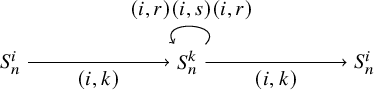
(iii) If both i and k must be in a simple path from r to s, it suffices to assume this path takes the form
 $(r,...,i,k,...,s)$
. In particular, the first piece
$(r,...,i,k,...,s)$
. In particular, the first piece
 $(r,...,i)$
is a path in
$(r,...,i)$
is a path in
 $\Gamma - k$
and the second piece
$\Gamma - k$
and the second piece
 $(k,...,s)$
is a path in
$(k,...,s)$
is a path in
 $\Gamma - i$
. Consider
$\Gamma - i$
. Consider
 $$\begin{align*}w(r,s) = w(i,k)(r,j)(i,k)(j,k)(k,s)(j,k)(i,k)(r,j)(i,k). \end{align*}$$
This sequence of transpositions gives a path from w to
 $w(r,s)$
in
$w(r,s)$
in
 $S_n^i\sqcup S_n^k$
. Below is a diagram detailing how each right multiplication moves between
$S_n^i\sqcup S_n^k$
. Below is a diagram detailing how each right multiplication moves between
 $S_n^i$
and
$S_n^i$
and
 $S_n^k$
:
$S_n^k$
:
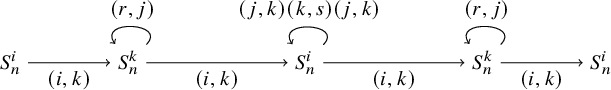
So subgraph with vertices
 $S_n^i\sqcup S_n^k$
is connected; our earlier assumption is verified and we have the claim.
$S_n^i\sqcup S_n^k$
is connected; our earlier assumption is verified and we have the claim.
7 Proof of the linear spanning theorem
This section shows that the collection
 $\mathcal {F}_\Gamma $
from Equation 5.1 (below Lemma 5.3) is a
$\mathcal {F}_\Gamma $
from Equation 5.1 (below Lemma 5.3) is a
 $\mathbb {C}$
-spanning set of
$\mathbb {C}$
-spanning set of
 $\mathcal {M}_{\Gamma }^1$
. In other words, we prove
$\mathcal {M}_{\Gamma }^1$
. In other words, we prove
 $\mathbb {C}\mathcal {F}_\Gamma = \mathcal {M}_{\Gamma }^1$
. First, we require a lemma on the compatibility of these splines on
$\mathbb {C}\mathcal {F}_\Gamma = \mathcal {M}_{\Gamma }^1$
. First, we require a lemma on the compatibility of these splines on
 $S_n$
with splines on
$S_n$
with splines on
 $S_{n-1}$
.
$S_{n-1}$
.
Lemma 7.1. Let
 $\Gamma $
on
$\Gamma $
on
 $[n]$
be cliqued and naturally labeled. Let
$[n]$
be cliqued and naturally labeled. Let ![]() . Then
. Then
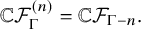 $$\begin{align*}\mathbb{C}\mathcal{F}_\Gamma^{(n)} = \mathbb{C}\mathcal{F}_{\Gamma-n}.\end{align*}$$
Proof. First, note that the Cayley graph
 $\mathcal {G}_{\Gamma - n}$
is equal to the induced subgraph of
$\mathcal {G}_{\Gamma - n}$
is equal to the induced subgraph of
 $\mathcal {G}_\Gamma $
with vertex set
$\mathcal {G}_\Gamma $
with vertex set
 $S_{n-1}$
. In particular, each element of
$S_{n-1}$
. In particular, each element of
 $\mathcal {F}_\Gamma ^{(n)}$
is in fact a spline in
$\mathcal {F}_\Gamma ^{(n)}$
is in fact a spline in
 $\mathcal {M}_{\Gamma - n}$
By Lemma 5.5(4), for each cut vertex j in
 $\Gamma $
and G the connected component of
$\Gamma $
and G the connected component of
 $\Gamma - j$
that contains n, we may remove the splines
$\Gamma - j$
that contains n, we may remove the splines
 $\{\bar {y}_{G,k}^j\vert _{S_{n-1}} \mid k \in [n]\}$
from
$\{\bar {y}_{G,k}^j\vert _{S_{n-1}} \mid k \in [n]\}$
from
 $\mathcal {F}_{\Gamma }^{(n)}$
without changing the
$\mathcal {F}_{\Gamma }^{(n)}$
without changing the
 $\mathbb {C}$
-span. Similarly, by Lemma 5.5(4), for each cut vertex
$\mathbb {C}$
-span. Similarly, by Lemma 5.5(4), for each cut vertex
 $j \neq n-1$
of
$j \neq n-1$
of
 $\Gamma - n$
and connected component G of
$\Gamma - n$
and connected component G of
 $(\Gamma - n)-j$
that contains
$(\Gamma - n)-j$
that contains
 $n-1$
, we may remove the splines
$n-1$
, we may remove the splines
 $\{\bar {y}_{G,k}^j \mid k \in [n]\}$
from
$\{\bar {y}_{G,k}^j \mid k \in [n]\}$
from
 $\mathcal {F}_{\Gamma -n}$
.
$\mathcal {F}_{\Gamma -n}$
.
Let
 $\bar {\rho } \in \mathcal {F}_{\Gamma }$
such that
$\bar {\rho } \in \mathcal {F}_{\Gamma }$
such that
 $\bar {\rho }\vert _{S_{n-1}}$
is a nonzero element of
$\bar {\rho }\vert _{S_{n-1}}$
is a nonzero element of
 $\mathcal {F}_\Gamma ^{(n)}$
. This means that
$\mathcal {F}_\Gamma ^{(n)}$
. This means that
 $\bar {\rho } \neq \bar {t}_n$
and
$\bar {\rho } \neq \bar {t}_n$
and
 $\bar {\rho } \neq \bar {x}_n$
. Additionally, by the definitions, if
$\bar {\rho } \neq \bar {x}_n$
. Additionally, by the definitions, if
 $\bar {\rho } = \bar {f}_A^s$
, we must have
$\bar {\rho } = \bar {f}_A^s$
, we must have
 $n \notin A$
(otherwise,
$n \notin A$
(otherwise,
 $\bar {\rho } \equiv 0$
) and
$\bar {\rho } \equiv 0$
) and
 $s \neq (n-1,n)$
, and if
$s \neq (n-1,n)$
, and if
 $\bar {\rho } = \bar {y}_{i,k}^j$
, then
$\bar {\rho } = \bar {y}_{i,k}^j$
, then
 $k \neq n$
. So we have a combinatorial description for the elements of
$k \neq n$
. So we have a combinatorial description for the elements of
 $\mathcal {F}_\Gamma ^{(n)}$
. In particular, as collections of functions from
$\mathcal {F}_\Gamma ^{(n)}$
. In particular, as collections of functions from
 $S_{n-1}$
to
$S_{n-1}$
to
 $\mathbb {C}[t_\bullet ]$
, we wish to show that the following two sets have the same
$\mathbb {C}[t_\bullet ]$
, we wish to show that the following two sets have the same
 $\mathbb {C}$
-span:
$\mathbb {C}$
-span:
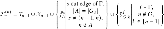 $$\begin{align*}\mathcal{F}_\Gamma^{(n)} =\mathcal{T}_{n-1} \cup \mathcal{X}_{n-1} \cup \left\{\bar{f}_A^s \left| \begin{matrix} s\text{ cut edge of }\Gamma,\\ \left| A \right| = \left| G_s \right| \\ s \neq (n-1,n), \\ n \notin A \end{matrix}\right.\right\} \cup \left\{\bar{y}_{G,k}^j \left| \begin{matrix}j \vdash \Gamma,\\ n \notin G,\\ k \in [n-1] \end{matrix}\right.\right\} \end{align*}$$
and
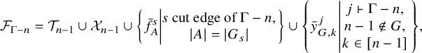 $$\begin{align*}\mathcal{F}_{\Gamma-n} = \mathcal{T}_{n-1} \cup \mathcal{X}_{n-1} \cup \left\{\bar{f}_A^s \left| \begin{matrix} s\text{ cut edge of }\Gamma-n,\\ \left| A \right| = \left| G_s \right|\end{matrix}\right.\right\} \cup \left\{\bar{y}_{G,k}^j \left| \begin{matrix}j \vdash \Gamma-n,\\ n-1 \notin G,\\ k \in [n-1] \end{matrix}\right.\right\}, \end{align*}$$
where for the cut edges
 $s = (i<j)$
of either
$s = (i<j)$
of either
 $\Gamma $
or
$\Gamma $
or
 $\Gamma - n$
, the component
$\Gamma - n$
, the component
 $G_s$
is the connected component of the graph with edge s removed that contains i.
$G_s$
is the connected component of the graph with edge s removed that contains i.
The equalities for
 $\bar {t}_i \in \mathcal {T}_{n-1}$
and
$\bar {t}_i \in \mathcal {T}_{n-1}$
and
 $\bar {x}_i\in \mathcal {X}_{n-1}$
are obvious, so we focus on the latter two subsets. The remainder of the proof is in three cases: whether the cliqued and naturally labeled graph
$\bar {x}_i\in \mathcal {X}_{n-1}$
are obvious, so we focus on the latter two subsets. The remainder of the proof is in three cases: whether the cliqued and naturally labeled graph
 $\Gamma $
is type A, B or C. Each argument amounts to matching the cut vertices and cut edges of
$\Gamma $
is type A, B or C. Each argument amounts to matching the cut vertices and cut edges of
 $\Gamma $
to those in
$\Gamma $
to those in
 $\Gamma - n$
(and vice versa). Each match gives pairs of splines in the third and fourth subsets above that are in fact equal to each other. Then we ensure that wherever these graph objects do not align, the ‘unmatched’ splines in each set are contained within the other’s
$\Gamma - n$
(and vice versa). Each match gives pairs of splines in the third and fourth subsets above that are in fact equal to each other. Then we ensure that wherever these graph objects do not align, the ‘unmatched’ splines in each set are contained within the other’s
 $\mathbb {C}$
-span.
$\mathbb {C}$
-span.
Type A: First, we compare the cut edges of
 $\Gamma $
and
$\Gamma $
and
 $\Gamma - n$
and ensure that each spline in the third subsets of both
$\Gamma - n$
and ensure that each spline in the third subsets of both
 $\mathcal {F}_{\Gamma }^{(n)}$
and
$\mathcal {F}_{\Gamma }^{(n)}$
and
 $\mathcal {F}_{\Gamma -n}$
are contained within the span of the other set. If
$\mathcal {F}_{\Gamma -n}$
are contained within the span of the other set. If
 $\Gamma $
is type A, then every cut edge of
$\Gamma $
is type A, then every cut edge of
 $\Gamma - n$
is also a cut edge of
$\Gamma - n$
is also a cut edge of
 $\Gamma $
. Every cut edge of
$\Gamma $
. Every cut edge of
 $\Gamma $
that is not
$\Gamma $
that is not
 $(n-1,n)$
is also a cut edge of
$(n-1,n)$
is also a cut edge of
 $\Gamma - n$
. Finally, if
$\Gamma - n$
. Finally, if
 $s = (i<j) \neq (n-1,n)$
is a cut edge, then the connected component of
$s = (i<j) \neq (n-1,n)$
is a cut edge, then the connected component of
 $([n] E(\Gamma ) \setminus \{s\})$
that contains i and the connected component of
$([n] E(\Gamma ) \setminus \{s\})$
that contains i and the connected component of
 $([n-1],E(\Gamma -n)\setminus \{s\})$
that contains i are equal, since these are the components with lower-valued vertices and thus are unaffected by removing n. So the third subsets in
$([n-1],E(\Gamma -n)\setminus \{s\})$
that contains i are equal, since these are the components with lower-valued vertices and thus are unaffected by removing n. So the third subsets in
 $\mathcal {F}_\Gamma ^{(n)}$
and
$\mathcal {F}_\Gamma ^{(n)}$
and
 $\mathcal {F}_{\Gamma - n}$
above are actually equal.
$\mathcal {F}_{\Gamma - n}$
above are actually equal.
Second, we compare the cut vertices and associated connected components of
 $\Gamma $
and
$\Gamma $
and
 $\Gamma - n$
and ensure that each spline in the fourth subsets of both
$\Gamma - n$
and ensure that each spline in the fourth subsets of both
 $\mathcal {F}_{\Gamma }^{(n)}$
and
$\mathcal {F}_{\Gamma }^{(n)}$
and
 $\mathcal {F}_{\Gamma -n}$
are contained within the span of the other set. There are two cases:
$\mathcal {F}_{\Gamma -n}$
are contained within the span of the other set. There are two cases:
 $\mathfrak {c}_{\Gamma }(n-1) = 1$
and
$\mathfrak {c}_{\Gamma }(n-1) = 1$
and
 $\mathfrak {c}_{\Gamma }(n-1)> 1$
. If
$\mathfrak {c}_{\Gamma }(n-1)> 1$
. If
 $\mathfrak {c}_{\Gamma }(n-1)> 1$
, every cut vertex in
$\mathfrak {c}_{\Gamma }(n-1)> 1$
, every cut vertex in
 $\Gamma $
is a cut vertex in
$\Gamma $
is a cut vertex in
 $\Gamma - n$
, and vice versa. If
$\Gamma - n$
, and vice versa. If
 $j \vdash \Gamma -n$
where
$j \vdash \Gamma -n$
where
 $j \neq n-1$
, if G is the component of
$j \neq n-1$
, if G is the component of
 $\Gamma - j$
that contains n then
$\Gamma - j$
that contains n then
 $G-n$
is the component of
$G-n$
is the component of
 $(\Gamma -n)-j$
that contains
$(\Gamma -n)-j$
that contains
 $n-1$
. If
$n-1$
. If
 $j = n-1$
, then
$j = n-1$
, then
 $\mathcal {F}_{\Gamma -n}$
contains every
$\mathcal {F}_{\Gamma -n}$
contains every
 $\bar {y}_{G,k}^{n-1}$
and
$\bar {y}_{G,k}^{n-1}$
and
 $\mathcal {F}_\Gamma ^{(n)}$
contains every
$\mathcal {F}_\Gamma ^{(n)}$
contains every
 $\bar {y}_{G,k}^{n-1}$
such that
$\bar {y}_{G,k}^{n-1}$
such that
 $n \notin G$
. Either way, these two collections of splines are identical, so the fourth subsets in
$n \notin G$
. Either way, these two collections of splines are identical, so the fourth subsets in
 $\mathcal {F}_{\Gamma }^{(n)}$
and
$\mathcal {F}_{\Gamma }^{(n)}$
and
 $\mathcal {F}_{\Gamma - n}$
are in fact equal.
$\mathcal {F}_{\Gamma - n}$
are in fact equal.
If
 $\mathfrak {c}_{\Gamma }(n-1) = 1$
, then
$\mathfrak {c}_{\Gamma }(n-1) = 1$
, then
 $n-1$
is not a cut vertex of
$n-1$
is not a cut vertex of
 $\Gamma -n$
, so
$\Gamma -n$
, so
 $\mathcal {F}_{\Gamma - n}$
does not contain the spline
$\mathcal {F}_{\Gamma - n}$
does not contain the spline
 $\bar {y}_{G,k}^{n-1} \in \mathcal {F}_\Gamma ^{(n)}$
where
$\bar {y}_{G,k}^{n-1} \in \mathcal {F}_\Gamma ^{(n)}$
where
 $V(G) = [n-2]$
. However, in this case, for all
$V(G) = [n-2]$
. However, in this case, for all
 $w \in S_{n-1}$
, we compute
$w \in S_{n-1}$
, we compute
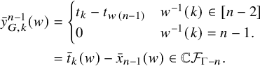 $$ \begin{align*} \bar{y}_{G,k}^{n-1}(w) &= \begin{cases} t_k - t_{w(n-1)} & w^{-1}(k) \in [n-2] \\ 0 & w^{-1}(k) = n-1. \end{cases}\\ &= \bar{t}_k(w) - \bar{x}_{n-1}(w) \in \mathbb{C}\mathcal{F}_{\Gamma-n}. \end{align*} $$
Every other cut vertex
 $j \vdash \Gamma - n$
and connected component G of
$j \vdash \Gamma - n$
and connected component G of
 $(\Gamma - n)-j$
(that does not contain
$(\Gamma - n)-j$
(that does not contain
 $n-1$
) is also a cut vertex of
$n-1$
) is also a cut vertex of
 $\Gamma $
and connected component of
$\Gamma $
and connected component of
 $\Gamma - j$
(that does not contain n), so each spline of the form
$\Gamma - j$
(that does not contain n), so each spline of the form
 $\bar {y}_{G,k}^j$
in
$\bar {y}_{G,k}^j$
in
 $\mathcal {F}_{\Gamma - n}$
has a direct counterpart in
$\mathcal {F}_{\Gamma - n}$
has a direct counterpart in
 $\mathcal {F}_\Gamma ^{(n)}$
. Thus
$\mathcal {F}_\Gamma ^{(n)}$
. Thus
 $\mathbb {C}\mathcal {F}_\Gamma ^{(n)} = \mathbb {C}\mathcal {F}_{\Gamma -n}$
, and the claim holds in type A.
$\mathbb {C}\mathcal {F}_\Gamma ^{(n)} = \mathbb {C}\mathcal {F}_{\Gamma -n}$
, and the claim holds in type A.
Type B: First, we compare the cut vertices and associated connected components to match elements in the fourth subsets. If
 $\Gamma $
is type B, then every cut vertex in
$\Gamma $
is type B, then every cut vertex in
 $\Gamma - n$
is also a cut vertex of
$\Gamma - n$
is also a cut vertex of
 $\Gamma $
, and for all
$\Gamma $
, and for all
 $j \vdash \Gamma $
, the connected component of
$j \vdash \Gamma $
, the connected component of
 $\Gamma - j$
that contains n also contains
$\Gamma - j$
that contains n also contains
 $n-1$
, so the fourth subsets in
$n-1$
, so the fourth subsets in
 $\mathcal {F}_\Gamma ^{(n)}$
and
$\mathcal {F}_\Gamma ^{(n)}$
and
 $\mathcal {F}_{\Gamma - n}$
are equal.
$\mathcal {F}_{\Gamma - n}$
are equal.
Now compare the cut edges to match elements in the third subsets. Every cut edge in
 $\Gamma $
is a cut edge in
$\Gamma $
is a cut edge in
 $\Gamma - n$
; however, the edge
$\Gamma - n$
; however, the edge
 $(n-2,n-1)$
is a cut edge in
$(n-2,n-1)$
is a cut edge in
 $\Gamma - n$
but not in
$\Gamma - n$
but not in
 $\Gamma $
. For this cut edge, we let
$\Gamma $
. For this cut edge, we let
 $G_{(n-2,n-1)}$
be the subgraph with vertex set
$G_{(n-2,n-1)}$
be the subgraph with vertex set
 $[n-2]$
. So
$[n-2]$
. So
 $\mathcal {F}_{\Gamma - n}$
has a subset
$\mathcal {F}_{\Gamma - n}$
has a subset
 $\left \{\bar {f}_{[n-1] \setminus k}^{(n-2,n-1)} \mid k \in [n-1]\right \}$
of splines that is not a subset of
$\left \{\bar {f}_{[n-1] \setminus k}^{(n-2,n-1)} \mid k \in [n-1]\right \}$
of splines that is not a subset of
 $\mathcal {F}_\Gamma ^{(n)}$
. We will show that these splines are contained within the span
$\mathcal {F}_\Gamma ^{(n)}$
. We will show that these splines are contained within the span
 $\mathbb {C}\mathcal {F}_\Gamma ^{(n)}$
. By Lemma 5.7 applied to the leaf
$\mathbb {C}\mathcal {F}_\Gamma ^{(n)}$
. By Lemma 5.7 applied to the leaf
 $(n-2,n-1)$
in
$(n-2,n-1)$
in
 $\Gamma -n$
, each spline in
$\Gamma -n$
, each spline in
 $\left \{\bar {f}_{[n-1] \setminus k}^{(n-2,n-1)}\in \mid k \in [n-1]\right \} \subset \mathcal {F}_{\Gamma -n}$
is a linear combination of the remaining splines in
$\left \{\bar {f}_{[n-1] \setminus k}^{(n-2,n-1)}\in \mid k \in [n-1]\right \} \subset \mathcal {F}_{\Gamma -n}$
is a linear combination of the remaining splines in
 $\mathcal {F}_{\Gamma -n}$
. Since the fourth subsets are equal and every other cut edge of
$\mathcal {F}_{\Gamma -n}$
. Since the fourth subsets are equal and every other cut edge of
 $\Gamma - n$
is a cut edge of
$\Gamma - n$
is a cut edge of
 $\Gamma $
, each of these remaining splines is also in
$\Gamma $
, each of these remaining splines is also in
 $\mathcal {F}_{\Gamma }^{(n)}$
. So the one subset
$\mathcal {F}_{\Gamma }^{(n)}$
. So the one subset
 $\left \{\bar {f}_{[n-1] \setminus k}^{(n-2,n-1)} \mid k \in [n-1]\right \}$
of unmatched splines in
$\left \{\bar {f}_{[n-1] \setminus k}^{(n-2,n-1)} \mid k \in [n-1]\right \}$
of unmatched splines in
 $\mathcal {F}_{\Gamma -n}$
is contained within the span
$\mathcal {F}_{\Gamma -n}$
is contained within the span
 $\mathbb {C}\mathcal {F}_\Gamma ^{(n)}$
, and so
$\mathbb {C}\mathcal {F}_\Gamma ^{(n)}$
, and so
 $\mathbb {C}\mathcal {F}_\Gamma ^{(n)} = \mathbb {C}\mathcal {F}_{\Gamma -n}$
.
$\mathbb {C}\mathcal {F}_\Gamma ^{(n)} = \mathbb {C}\mathcal {F}_{\Gamma -n}$
.
Type C: If
 $\Gamma $
is type C, then every cut vertex or edge in
$\Gamma $
is type C, then every cut vertex or edge in
 $\Gamma -n$
is also a cut vertex or edge in
$\Gamma -n$
is also a cut vertex or edge in
 $\Gamma $
, and vice versa. Additionally, for any
$\Gamma $
, and vice versa. Additionally, for any
 $j \vdash \Gamma $
, the connected component of
$j \vdash \Gamma $
, the connected component of
 $\Gamma - j$
containing n also contains
$\Gamma - j$
containing n also contains
 $n-1$
. So all indexing data is the same, and so
$n-1$
. So all indexing data is the same, and so
 $\mathcal {F}_{\Gamma }^{(n)} = \mathcal {F}_{\Gamma -n}$
. Thus, the claim holds in Type C.
$\mathcal {F}_{\Gamma }^{(n)} = \mathcal {F}_{\Gamma -n}$
. Thus, the claim holds in Type C.
The proof of Theorem 7.2 below assumes a natural label, so we will use the indexing conventions for
 $\mathcal {F}_\Gamma $
described in Subsection 6.1. In particular, we will heavily use the weakly dominant
$\mathcal {F}_\Gamma $
described in Subsection 6.1. In particular, we will heavily use the weakly dominant
 $(i,j)> \Gamma $
and strongly dominant
$(i,j)> \Gamma $
and strongly dominant
 $(i,j) \gg \Gamma $
pairs in Definition 6.5. Now we are able to prove that
$(i,j) \gg \Gamma $
pairs in Definition 6.5. Now we are able to prove that
 $\mathbb {C}\mathcal {F}_\Gamma = \mathcal {M}_{\Gamma }^1$
and compute a recursive dimension formula.
$\mathbb {C}\mathcal {F}_\Gamma = \mathcal {M}_{\Gamma }^1$
and compute a recursive dimension formula.
Theorem 7.2. Let
 $\Gamma $
be a connected graph. The splines
$\Gamma $
be a connected graph. The splines
 $\mathcal {F}_\Gamma $
from Equation (5.1) form a
$\mathcal {F}_\Gamma $
from Equation (5.1) form a
 $\mathbb {C}$
-spanning set of
$\mathbb {C}$
-spanning set of
 $\mathcal {M}_{\Gamma }^1$
. Furthermore, if
$\mathcal {M}_{\Gamma }^1$
. Furthermore, if
 $\Gamma $
is cliqued and naturally labeled, then
$\Gamma $
is cliqued and naturally labeled, then
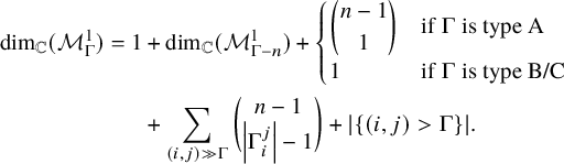 $$ \begin{align*} \dim_{\mathbb{C}}(\mathcal{M}_{\Gamma}^1) = 1&+\dim_{\mathbb{C}}(\mathcal{M}_{\Gamma-n}^1) + \begin{cases} \genfrac(){0pt}{0}{n-1}{1} &\text{if }\Gamma \; \text{is type A} \\ 1 &\text{if }\Gamma \; \text{is type B/C} \end{cases} \\&+ \sum_{(i,j) \gg \Gamma} \genfrac(){0pt}{0}{n-1}{\left| \Gamma_i^j \right|-1} + \left| \left\{(i,j)> \Gamma \right\} \right|. \end{align*} $$
Proof. It suffices to assume for both parts of the claim that
 $\Gamma $
is cliqued and naturally labeled. Recall the decomposition
$\Gamma $
is cliqued and naturally labeled. Recall the decomposition
 $S_n = S_{n}^1 \sqcup \cdots \sqcup S_n^{n}$
, where
$S_n = S_{n}^1 \sqcup \cdots \sqcup S_n^{n}$
, where ![]() . Note
. Note
 $S_n^n = S_{n-1}$
. Let
$S_n^n = S_{n-1}$
. Let
 $\bar {\rho } \in \mathcal {M}_{\Gamma }^1$
. We will prove that
$\bar {\rho } \in \mathcal {M}_{\Gamma }^1$
. We will prove that
 $\bar {\rho } \in \mathbb {C}\mathcal {F}_\Gamma $
and proceed by induction on n. The base case is
$\bar {\rho } \in \mathbb {C}\mathcal {F}_\Gamma $
and proceed by induction on n. The base case is
 $n=3$
, where
$n=3$
, where
 $\mathcal {M}_{\Gamma } = \mathbb {C}\mathcal {F}_\Gamma $
is easily verified by hand (there are only two connected graphs on three vertices) and either way follows from [Reference Ayzenberg, Masuda and Sato4].
$\mathcal {M}_{\Gamma } = \mathbb {C}\mathcal {F}_\Gamma $
is easily verified by hand (there are only two connected graphs on three vertices) and either way follows from [Reference Ayzenberg, Masuda and Sato4].
In each of the three steps to the proof given below, we use elements of
 $\mathcal {F}_\Gamma $
to replace
$\mathcal {F}_\Gamma $
to replace
 $\bar {\rho }$
with a spline supported on a strictly smaller subset of
$\bar {\rho }$
with a spline supported on a strictly smaller subset of
 $S_n$
. To track
$S_n$
. To track
 $\dim _{\mathbb {C}}(\mathcal {M}_{\Gamma }^1)$
, we will create a set
$\dim _{\mathbb {C}}(\mathcal {M}_{\Gamma }^1)$
, we will create a set
 $\mathcal {B}$
of linearly independent elements of
$\mathcal {B}$
of linearly independent elements of
 $\mathcal {M}_{\Gamma }^1$
.
$\mathcal {M}_{\Gamma }^1$
.
 $\left (\textbf {Step 1: }S_n^n\right )$
This step applies the induction assumption to replace
$\left (\textbf {Step 1: }S_n^n\right )$
This step applies the induction assumption to replace
 $\bar {\rho }$
with a spline supported on
$\bar {\rho }$
with a spline supported on
 $S_n^1 \sqcup \cdots \sqcup S_n^{n-1}$
. If
$S_n^1 \sqcup \cdots \sqcup S_n^{n-1}$
. If
 $w,v \in S_n^n = S_{n-1}$
with
$w,v \in S_n^n = S_{n-1}$
with
 $w^{-1}v = (i,j) \in E(\Gamma - n)$
, then
$w^{-1}v = (i,j) \in E(\Gamma - n)$
, then
 $\bar {\rho }(w) - \bar {\rho }(v) = c\left (t_{w(i)}-t_{w(j)}\right )$
, where
$\bar {\rho }(w) - \bar {\rho }(v) = c\left (t_{w(i)}-t_{w(j)}\right )$
, where
 $c \in \mathbb {C}$
. Since
$c \in \mathbb {C}$
. Since
 $w(i) \neq n$
and
$w(i) \neq n$
and
 $w(j) \neq n$
, the coefficient
$w(j) \neq n$
, the coefficient
 $[t_n]\bar {\rho }(w)$
of
$[t_n]\bar {\rho }(w)$
of
 $t_n$
in
$t_n$
in
 $\bar {\rho }(w)$
must be equal to
$\bar {\rho }(w)$
must be equal to
 $[t_n]\bar {\rho }(v)$
. Since
$[t_n]\bar {\rho }(v)$
. Since
 $\Gamma - n$
is connected, the induced subgraph of
$\Gamma - n$
is connected, the induced subgraph of
 $\mathcal {G}_\Gamma $
with vertex set
$\mathcal {G}_\Gamma $
with vertex set
 $S_n^n$
is connected. Moreover, the coefficient of
$S_n^n$
is connected. Moreover, the coefficient of
 $t_n$
is the same for all
$t_n$
is the same for all
 $\bar {\rho }(u)$
, where
$\bar {\rho }(u)$
, where
 $u \in S_n^n$
. Let
$u \in S_n^n$
. Let ![]() for
for
 $u \in S_n^n$
. Then
$u \in S_n^n$
. Then
 $[t_n]\left (\bar {\rho }-c_n\bar {t}_n\right )(u) = 0$
for all
$[t_n]\left (\bar {\rho }-c_n\bar {t}_n\right )(u) = 0$
for all
 $u \in S_{n-1}$
.
$u \in S_{n-1}$
.
So we replace
 $\bar {\rho }$
with
$\bar {\rho }$
with
 $\bar {\rho } - c_n\bar {t}_n$
, and now
$\bar {\rho } - c_n\bar {t}_n$
, and now
 $\bar {\rho }(u) \in \mathbb {C}[t_1,\ldots ,t_{n-1}]$
when
$\bar {\rho }(u) \in \mathbb {C}[t_1,\ldots ,t_{n-1}]$
when
 $u \in S_n^n$
. Let
$u \in S_n^n$
. Let ![]() . We will add linearly independent elements to
. We will add linearly independent elements to
 $\mathcal {B}$
throughout the proof and keep track of
$\mathcal {B}$
throughout the proof and keep track of
 $\left | \mathcal {B} \right |$
.
$\left | \mathcal {B} \right |$
.
By Lemma 7.1 and the induction hypothesis,
 $\mathcal {M}_{\Gamma -n}^1 = \mathbb {C}\mathcal {F}_{\Gamma -n} = \mathbb {C}\mathcal {F}_\Gamma ^{(n)}$
. So we may assume that
$\mathcal {M}_{\Gamma -n}^1 = \mathbb {C}\mathcal {F}_{\Gamma -n} = \mathbb {C}\mathcal {F}_\Gamma ^{(n)}$
. So we may assume that
 $\bar {\rho }\vert _{S_{n-1}} \equiv 0$
. Add to
$\bar {\rho }\vert _{S_{n-1}} \equiv 0$
. Add to
 $\mathcal {B}$
the
$\mathcal {B}$
the
 $\dim _{\mathbb {C}}(\mathcal {M}_{\Gamma -n}^1)$
-many splines required. Note these splines are independent once restricted to
$\dim _{\mathbb {C}}(\mathcal {M}_{\Gamma -n}^1)$
-many splines required. Note these splines are independent once restricted to
 $S_n^n = S_{n-1}$
, so any nontrivial linear combination will have elements of
$S_n^n = S_{n-1}$
, so any nontrivial linear combination will have elements of
 $S_n^n$
in its support. At this point,
$S_n^n$
in its support. At this point,
 $\left | \mathcal {B} \right | = \dim _{\mathbb {C}}(\mathcal {M}_{\Gamma - n}^1)+1$
, and
$\left | \mathcal {B} \right | = \dim _{\mathbb {C}}(\mathcal {M}_{\Gamma - n}^1)+1$
, and
 $\bar {\rho } \equiv 0$
on
$\bar {\rho } \equiv 0$
on
 $S_n^n$
.
$S_n^n$
.
 $\left (\textbf {Step 2: } S_n^{n-1}\right )$
Next, we use elements of
$\left (\textbf {Step 2: } S_n^{n-1}\right )$
Next, we use elements of
 $\mathcal {F}_\Gamma $
to replace
$\mathcal {F}_\Gamma $
to replace
 $\bar {\rho }$
with a spline that evaluates to
$\bar {\rho }$
with a spline that evaluates to
 $0$
on
$0$
on
 $S_n^{n-1} \sqcup S_n^n$
. The process is slightly different for graphs of type A and types
$S_n^{n-1} \sqcup S_n^n$
. The process is slightly different for graphs of type A and types
 $B/C$
.
$B/C$
.
Since
 $\Gamma $
is cliqued and naturally labeled,
$\Gamma $
is cliqued and naturally labeled,
 $(n-1,n) \in E(\Gamma )$
. Thus, for all
$(n-1,n) \in E(\Gamma )$
. Thus, for all
 $w \in S_n^{n-1}$
, there is an edge
$w \in S_n^{n-1}$
, there is an edge
 $(w,w(n-1,n)) \in E(\mathcal {G}_\Gamma )$
where
$(w,w(n-1,n)) \in E(\mathcal {G}_\Gamma )$
where
 $w(n-1,n) \in S_n^n$
. Each of these edges are labeled
$w(n-1,n) \in S_n^n$
. Each of these edges are labeled
 $\left \langle t_{w(n-1)}-t_{w(n)}\right \rangle = \left \langle t_n-t_{w(n)}\right \rangle $
. Since
$\left \langle t_{w(n-1)}-t_{w(n)}\right \rangle = \left \langle t_n-t_{w(n)}\right \rangle $
. Since
 $\bar {\rho }\equiv 0$
on
$\bar {\rho }\equiv 0$
on
 $S_n^n$
, we have that
$S_n^n$
, we have that
 $\bar {\rho }(w) = c_w\left (t_n-t_{w(n)}\right )$
for some
$\bar {\rho }(w) = c_w\left (t_n-t_{w(n)}\right )$
for some
 $c_w \in \mathbb {C}$
for all
$c_w \in \mathbb {C}$
for all
 $w \in S_n^{n-1}$
.
$w \in S_n^{n-1}$
.
Type A: By Lemma 6.13, if
 $w,v \in S_n^{n-1}$
and
$w,v \in S_n^{n-1}$
and
 $w(n) = v(n)$
, then
$w(n) = v(n)$
, then
 $c_w=c_v$
. Let
$c_w=c_v$
. Let ![]() when
when
 $w(n) = k$
. If
$w(n) = k$
. If
 $w(n-1) = n$
and
$w(n-1) = n$
and
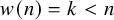 $w(n) = k < n$
, then by definition,
$w(n) = k < n$
, then by definition,
 $\bar {f}_{[n] \setminus \{k\}}^{(n-1,n)}(w) = t_n-t_{w(n)}$
. However, if
$\bar {f}_{[n] \setminus \{k\}}^{(n-1,n)}(w) = t_n-t_{w(n)}$
. However, if
 $w(n) = n$
, then
$w(n) = n$
, then
 $\bar {f}_{[n] \setminus \{k\}}^{(n-1,n)}(w) = 0$
whenever
$\bar {f}_{[n] \setminus \{k\}}^{(n-1,n)}(w) = 0$
whenever
 $k \neq n$
. It follows that
$k \neq n$
. It follows that
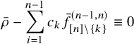 $$\begin{align*}\bar{\rho} - \sum_{i=1}^{n-1}c_k \bar{f}_{[n] \setminus \{k\}}^{(n-1,n)} \equiv 0\end{align*}$$
on
 $S_n^{n-1}\sqcup S_n^n$
. Add the
$S_n^{n-1}\sqcup S_n^n$
. Add the
 $n-1$
coset splines
$n-1$
coset splines
 $\bar {f}_{[n] \setminus \{k\}}^{(n-1,n)}$
used above to
$\bar {f}_{[n] \setminus \{k\}}^{(n-1,n)}$
used above to
 $\mathcal {B}$
, which are linearly independent from the splines already in
$\mathcal {B}$
, which are linearly independent from the splines already in
 $\mathcal {B}$
since they are not supported on
$\mathcal {B}$
since they are not supported on
 $S_n^n$
and have disjoint support on
$S_n^n$
and have disjoint support on
 $S_n^{n-1}$
. In type A, at this point,
$S_n^{n-1}$
. In type A, at this point,
 $\left | \mathcal {B} \right | = 1 +\dim _{\mathbb {C}}(\mathcal {M}_{\Gamma - n}^1) + \genfrac (){0pt}{0}{n-1}{1}$
, and
$\left | \mathcal {B} \right | = 1 +\dim _{\mathbb {C}}(\mathcal {M}_{\Gamma - n}^1) + \genfrac (){0pt}{0}{n-1}{1}$
, and
 $\mathcal {B}$
is linearly independent, even if we restrict the splines in
$\mathcal {B}$
is linearly independent, even if we restrict the splines in
 $\mathcal {B}$
to
$\mathcal {B}$
to
 $S_n^{n-1} \sqcup S_n^n$
.
$S_n^{n-1} \sqcup S_n^n$
.
Type B/C: We proceed in the same format as type A. By Lemma 6.13, if
 $w,v \in S_n^{n-1}$
, then
$w,v \in S_n^{n-1}$
, then
 $c_w=c_v$
. Write
$c_w=c_v$
. Write ![]() for
for
 $w \in S_n^{n-1}$
. Then
$w \in S_n^{n-1}$
. Then
 $$\begin{align*}\bar{\rho} - c(\bar{t}_n - \bar{x}_n) \equiv 0\end{align*}$$
on
 $S_n^{n-1}\sqcup S_n^n$
. Add the single linearly independent spline
$S_n^{n-1}\sqcup S_n^n$
. Add the single linearly independent spline
 $\bar {t}_n - \bar {x}_n$
to
$\bar {t}_n - \bar {x}_n$
to
 $\mathcal {B}$
. In type B/C at this point,
$\mathcal {B}$
. In type B/C at this point,
 $\left | \mathcal {B} \right | = \dim _{\mathbb {C}}(\mathcal {M}_{\Gamma - n}^1) + 2$
, and
$\left | \mathcal {B} \right | = \dim _{\mathbb {C}}(\mathcal {M}_{\Gamma - n}^1) + 2$
, and
 $\mathcal {B}$
is linearly independent, even if we restrict each spline to
$\mathcal {B}$
is linearly independent, even if we restrict each spline to
 $S_n^{n-1} \sqcup S_n^n$
.
$S_n^{n-1} \sqcup S_n^n$
.
 $\left (\textbf {Step 3: } S_n^i\right )$
Now given a spline
$\left (\textbf {Step 3: } S_n^i\right )$
Now given a spline
 $\bar {\rho }$
such that
$\bar {\rho }$
such that
 $\bar {\rho } \equiv 0$
on
$\bar {\rho } \equiv 0$
on
 $S_n^{i+1} \sqcup \cdots S_n^n$
, we show how to replace it with a spline that vanishes on
$S_n^{i+1} \sqcup \cdots S_n^n$
, we show how to replace it with a spline that vanishes on
 $S_n^i \sqcup \cdots S_n^n$
. This step is repeated until
$S_n^i \sqcup \cdots S_n^n$
. This step is repeated until
 $\bar {\rho }$
vanishes on all of
$\bar {\rho }$
vanishes on all of
 $S_n$
. Assume that
$S_n$
. Assume that
 $\bar {\rho } \equiv 0$
on
$\bar {\rho } \equiv 0$
on
 $S_n^{i+1} \sqcup \cdots \sqcup S_n^n$
. Additionally, we assume that the splines in
$S_n^{i+1} \sqcup \cdots \sqcup S_n^n$
. Additionally, we assume that the splines in
 $\mathcal {B}$
are linearly independent; moreover, the set remains linearly independent once each spline is restricted to
$\mathcal {B}$
are linearly independent; moreover, the set remains linearly independent once each spline is restricted to
 $S_n^{i+1} \sqcup \cdots \sqcup S_n^n$
. In particular, any nontrivial linear combination of splines in
$S_n^{i+1} \sqcup \cdots \sqcup S_n^n$
. In particular, any nontrivial linear combination of splines in
 $\mathcal {B}$
is nonzero on
$\mathcal {B}$
is nonzero on
 $S_n^{i+1} \sqcup \cdots \sqcup S_n^n$
(and therefore
$S_n^{i+1} \sqcup \cdots \sqcup S_n^n$
(and therefore
 $S_n$
). The remainder of the proof is type A/B/C-independent but still requires three cases.
$S_n$
). The remainder of the proof is type A/B/C-independent but still requires three cases.
First, a formulation of
 $\bar {\rho }(w)$
for
$\bar {\rho }(w)$
for
 $w \in S_n^i$
will be used in each case. Since
$w \in S_n^i$
will be used in each case. Since
 $\Gamma $
is naturally labeled and
$\Gamma $
is naturally labeled and
 $i \neq n$
, there exists
$i \neq n$
, there exists
 $j \in [n]$
such that
$j \in [n]$
such that
 $i<j$
and
$i<j$
and
 $(i,j) \in E(\Gamma )$
, so
$(i,j) \in E(\Gamma )$
, so
 $(w,w(i,j)) \in E(\mathcal {G}_\Gamma )$
. If
$(w,w(i,j)) \in E(\mathcal {G}_\Gamma )$
. If
 $w \in S_n^i$
, then
$w \in S_n^i$
, then
 $w(i,j) \in S_n^j$
, so
$w(i,j) \in S_n^j$
, so
 $$\begin{align*}\bar{\rho}(w) = c_w(t_{w(i)} - t_{w(j)}) = c_w(t_n-t_{w(j)})\end{align*}$$
for some
 $c_w \in \mathbb {C}$
.
$c_w \in \mathbb {C}$
.
Case 1: If i is not j-dominant for any
 $j \in [n]$
, since
$j \in [n]$
, since
 $\Gamma $
is naturally labeled, there exist (at least) two vertices
$\Gamma $
is naturally labeled, there exist (at least) two vertices
 $j,k$
where
$j,k$
where
 $i < j<k$
and
$i < j<k$
and
 $\{(i,j),(i,k)\}\subset E(\Gamma )$
. It follows that
$\{(i,j),(i,k)\}\subset E(\Gamma )$
. It follows that
 $$\begin{align*}\bar{\rho}(w) = c_w\left(t_n-t_{w(j)}\right) = c^{\prime}_w\left(t_n-t_{w(k)}\right).\end{align*}$$
This is not possible for
 $c_w,c^{\prime }_w \in \mathbb {C}$
unless
$c_w,c^{\prime }_w \in \mathbb {C}$
unless
 $c_w=c^{\prime }_w=0$
, and so
$c_w=c^{\prime }_w=0$
, and so
 $\bar {\rho }(w) = 0$
. In short,
$\bar {\rho }(w) = 0$
. In short,
 $\bar {\rho } \equiv 0$
on
$\bar {\rho } \equiv 0$
on
 $S_n^i$
, and we do not need any splines from
$S_n^i$
, and we do not need any splines from
 $\mathcal {F}_\Gamma $
to achieve this.
$\mathcal {F}_\Gamma $
to achieve this.
Case 2: If there exists
 $j \in [n]$
where
$j \in [n]$
where
 $(i,j) \gg \Gamma $
, then i is the maximal vertex in its connected component of
$(i,j) \gg \Gamma $
, then i is the maximal vertex in its connected component of
 $\Gamma - j$
. Thus, the vertex j is the only element in the neighborhood
$\Gamma - j$
. Thus, the vertex j is the only element in the neighborhood
 $N(i)$
of the vertex i that is greater than i (so i is not k-dominant for any
$N(i)$
of the vertex i that is greater than i (so i is not k-dominant for any
 $k \neq j$
), and
$k \neq j$
), and
 $(i,j)$
is a cut edge of
$(i,j)$
is a cut edge of
 $\Gamma $
. By Lemma 6.14, if
$\Gamma $
. By Lemma 6.14, if
 $v \in w\langle E(\Gamma )\setminus (i,j)\rangle $
, then
$v \in w\langle E(\Gamma )\setminus (i,j)\rangle $
, then
 $c_v=c_w$
.
$c_v=c_w$
.
Recall that
 $v \in w\langle E(\Gamma )\setminus (i,j)\rangle $
if and only if
$v \in w\langle E(\Gamma )\setminus (i,j)\rangle $
if and only if
 $w(V(\Gamma _i^j)) = v(V(\Gamma _i^j))$
. Let
$w(V(\Gamma _i^j)) = v(V(\Gamma _i^j))$
. Let
and write ![]() if
if
 $w(V(\Gamma _i^j)) = A$
. If
$w(V(\Gamma _i^j)) = A$
. If
 $w(i) = n$
, then
$w(i) = n$
, then
 $w^{-1}(V(\Gamma _i^j)) = A \in \mathcal {A}$
, and we compute
$w^{-1}(V(\Gamma _i^j)) = A \in \mathcal {A}$
, and we compute
 $\bar {f}_{A}^{(i,j)}(w) = t_n - t_{w(j)}$
. Also, since
$\bar {f}_{A}^{(i,j)}(w) = t_n - t_{w(j)}$
. Also, since
 $\Gamma $
is naturally labeled, if
$\Gamma $
is naturally labeled, if
 $k>i$
, then
$k>i$
, then
 $k \notin \Gamma _i^j$
. In particular, if
$k \notin \Gamma _i^j$
. In particular, if
 $k>i$
and
$k>i$
and
 $w(k) = n$
, then
$w(k) = n$
, then
 $w^{-1}(V(\Gamma _i^j)) \notin \mathcal {A}$
, and so
$w^{-1}(V(\Gamma _i^j)) \notin \mathcal {A}$
, and so
 $\bar {f}_A^{(i,j)}(w) = 0$
for all
$\bar {f}_A^{(i,j)}(w) = 0$
for all
 $w \in S_n^{i+1} \sqcup \cdots \sqcup s_n^n$
. It follows that
$w \in S_n^{i+1} \sqcup \cdots \sqcup s_n^n$
. It follows that
 $$\begin{align*}\bar{\rho} - \sum_{A \in \mathcal{A}} c_A \bar{f}_A^{(i,j)} \equiv 0\end{align*}$$
on
 $S_n^i \sqcup \cdots \sqcup S_n^n$
. We replace
$S_n^i \sqcup \cdots \sqcup S_n^n$
. We replace
 $\bar {\rho }$
with this spline. The coset splines
$\bar {\rho }$
with this spline. The coset splines
 $\bar {f}_A^{(i,j)}$
for
$\bar {f}_A^{(i,j)}$
for
 $A \in \mathcal {A}$
have disjoint support among themselves and are only supported on
$A \in \mathcal {A}$
have disjoint support among themselves and are only supported on
 $S_n^r$
for
$S_n^r$
for
 $r \leq i$
, so
$r \leq i$
, so
 $\{\bar {f}_A^{(i,j)} \mid A \in \mathcal {A}\} \cup \mathcal {B}$
is linearly independent, even when each spline is restricted to
$\{\bar {f}_A^{(i,j)} \mid A \in \mathcal {A}\} \cup \mathcal {B}$
is linearly independent, even when each spline is restricted to
 $S_n^i \sqcup \cdots \sqcup S_n^n$
. Each time we use Case 2 (i.e., for each
$S_n^i \sqcup \cdots \sqcup S_n^n$
. Each time we use Case 2 (i.e., for each
 $(i,j) \gg \Gamma $
), we add
$(i,j) \gg \Gamma $
), we add
 $\left | \mathcal {A} \right | = \genfrac (){0pt}{0}{n-1}{\left | \Gamma _i^j \right |-1}$
-many splines to
$\left | \mathcal {A} \right | = \genfrac (){0pt}{0}{n-1}{\left | \Gamma _i^j \right |-1}$
-many splines to
 $\mathcal {B}$
.
$\mathcal {B}$
.
Case 3: If there exists
 $j \in [n]$
where
$j \in [n]$
where
 $(i,j)> \Gamma $
, the vertex j is the only element in the neighborhood
$(i,j)> \Gamma $
, the vertex j is the only element in the neighborhood
 $N(i)$
of the vertex i that is greater than i (so i is not k-dominant for any
$N(i)$
of the vertex i that is greater than i (so i is not k-dominant for any
 $k \neq j$
), but
$k \neq j$
), but
 $(i,j)$
is not a cut edge. By Lemma 6.15, if
$(i,j)$
is not a cut edge. By Lemma 6.15, if
 $w,v \in S_n^i$
, then
$w,v \in S_n^i$
, then ![]() . Finally, we confirm that
. Finally, we confirm that
 $$\begin{align*}\bar{\rho} - c\, \bar{y}_{i,n}^j \equiv 0\end{align*}$$
on
 $S_n^i \sqcup \cdots \sqcup S_n^n$
. We replace
$S_n^i \sqcup \cdots \sqcup S_n^n$
. We replace
 $\bar {\rho }$
with this spline. The single spline
$\bar {\rho }$
with this spline. The single spline
 $\bar {y}_{i,n}^j$
is supported on
$\bar {y}_{i,n}^j$
is supported on
 $S_n^r$
for
$S_n^r$
for
 $r \leq i$
, and so
$r \leq i$
, and so
 $\{\bar {y}_{i,n}^j\} \cup \mathcal {B}$
is linearly independent, even when restricted to
$\{\bar {y}_{i,n}^j\} \cup \mathcal {B}$
is linearly independent, even when restricted to
 $S_n^i \sqcup \cdots \sqcup S_n^n$
. Each time Case 3 is used (i.e., for each
$S_n^i \sqcup \cdots \sqcup S_n^n$
. Each time Case 3 is used (i.e., for each
 $(i,j)> \Gamma $
), we add
$(i,j)> \Gamma $
), we add
 $1$
spline to
$1$
spline to
 $\mathcal {B}$
.
$\mathcal {B}$
.
When
 $i=1$
is reached, we have used
$i=1$
is reached, we have used
 $\mathcal {F}_\Gamma $
to replace
$\mathcal {F}_\Gamma $
to replace
 $\bar {\rho }$
with a spline
$\bar {\rho }$
with a spline
 $\bar {\rho } \equiv 0$
on all of
$\bar {\rho } \equiv 0$
on all of
 $S_n$
. Thus,
$S_n$
. Thus,
 $\bar {\rho } \in \mathbb {C}\mathcal {B}$
, and the set
$\bar {\rho } \in \mathbb {C}\mathcal {B}$
, and the set
 $\mathcal {B} \subseteq \mathcal {F}_\Gamma $
is linearly independent (the restriction is now to the whole symmetric group
$\mathcal {B} \subseteq \mathcal {F}_\Gamma $
is linearly independent (the restriction is now to the whole symmetric group
 $S_n^1 \sqcup \cdots \sqcup S_n^n = S_n$
), and
$S_n^1 \sqcup \cdots \sqcup S_n^n = S_n$
), and
 $\left | \mathcal {B} \right | = \dim _{\mathbb {C}}(\mathcal {M}_{\Gamma }^1)$
is as claimed.
$\left | \mathcal {B} \right | = \dim _{\mathbb {C}}(\mathcal {M}_{\Gamma }^1)$
is as claimed.
8 The linear dimension formula
This section constructs a combinatorial invariant of simple graphs that is also the
 $\mathbb {C}$
-dimension of the associated linear splines.
$\mathbb {C}$
-dimension of the associated linear splines.
Let
 $\Gamma $
be a connected graph on at least three vertices. First, if
$\Gamma $
be a connected graph on at least three vertices. First, if
 $j \vdash \Gamma $
is a cut vertex, let
$j \vdash \Gamma $
is a cut vertex, let
 $\mathfrak {c}_\Gamma (j)+1$
be the number of connected components in
$\mathfrak {c}_\Gamma (j)+1$
be the number of connected components in
 $\Gamma - j$
. This is a straightforward expansion of the definition we gave for
$\Gamma - j$
. This is a straightforward expansion of the definition we gave for
 $\mathfrak {c}_\Gamma (j)$
from naturally labeled graphs to all graphs. When
$\mathfrak {c}_\Gamma (j)$
from naturally labeled graphs to all graphs. When
 $\Gamma $
is fixed, we may drop the subscript and write
$\Gamma $
is fixed, we may drop the subscript and write
 $\mathfrak {c}(j)$
.
$\mathfrak {c}(j)$
.
Definition 8.1. Recall the construction of a block-cut tree in Definition 6.2. In this tree, every leaf is a block of
 $\Gamma $
. Let
$\Gamma $
. Let
 $\mathrm {LB}_\Gamma $
be the set of blocks in
$\mathrm {LB}_\Gamma $
be the set of blocks in
 $\Gamma $
that are leaves in the block-cut tree. We call elements of
$\Gamma $
that are leaves in the block-cut tree. We call elements of
 $\mathrm {LB}_\Gamma $
leaf blocks of
$\mathrm {LB}_\Gamma $
leaf blocks of
 $\Gamma $
. Let
$\Gamma $
. Let
 $\mathrm {IB}_\Gamma $
be the set of blocks in
$\mathrm {IB}_\Gamma $
be the set of blocks in
 $\Gamma $
that are not leaves in the block-cut tree. We call elements of
$\Gamma $
that are not leaves in the block-cut tree. We call elements of
 $\mathrm {IB}_\Gamma $
internal blocks of
$\mathrm {IB}_\Gamma $
internal blocks of
 $\Gamma $
. Note when
$\Gamma $
. Note when
 $\Gamma $
is
$\Gamma $
is
 $2$
-connected,
$2$
-connected,
 $\mathrm {LB}_\Gamma = \emptyset $
and
$\mathrm {LB}_\Gamma = \emptyset $
and
 $\mathrm {IB}_\Gamma = \{\Gamma \}$
; in particular, when the block-cut tree of
$\mathrm {IB}_\Gamma = \{\Gamma \}$
; in particular, when the block-cut tree of
 $\Gamma $
is a single vertex (i.e., when
$\Gamma $
is a single vertex (i.e., when
 $\Gamma $
is
$\Gamma $
is
 $2$
-connected), we consider
$2$
-connected), we consider
 $\Gamma $
to be an internal block.
$\Gamma $
to be an internal block.
If a block B in
 $\Gamma $
is size
$\Gamma $
is size
 $\left | B \right | = 2$
, that block must consist of two vertices in
$\left | B \right | = 2$
, that block must consist of two vertices in
 $\Gamma $
connected by an edge. Since blocks are maximal
$\Gamma $
connected by an edge. Since blocks are maximal
 $2$
-connected subgraphs, this edge must be a cut edge. In particular, blocks B in
$2$
-connected subgraphs, this edge must be a cut edge. In particular, blocks B in
 $\mathrm {IB}_\Gamma $
of size
$\mathrm {IB}_\Gamma $
of size
 $\left | B \right | = 2$
are in bijection with cut edges of
$\left | B \right | = 2$
are in bijection with cut edges of
 $\Gamma $
that are not leaf edges. Let
$\Gamma $
that are not leaf edges. Let ![]() . The elements of
. The elements of
 $\mathrm {IC}_\Gamma $
are internal cut edges of
$\mathrm {IC}_\Gamma $
are internal cut edges of
 $\Gamma $
.
$\Gamma $
.
Example 8.2. Consider the graph
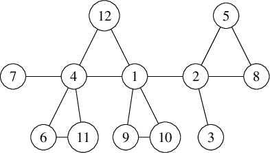
with block-cut tree
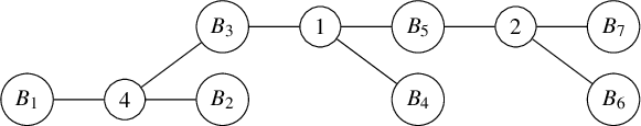
This is the construction from the beginning of Example 6.4. The leaf blocks are
 $$\begin{align*}\mathrm{LB}_\Gamma = \left\{ B_1,B_2,B_4,B_6,B_7 \right\}.\end{align*}$$
The internal blocks are
 $$\begin{align*}\mathrm{IB}_\Gamma = \left\{B_3,B_5 \right\}.\end{align*}$$
Within those internal blocks,
 $\left | B_5 \right | = 2$
and
$\left | B_5 \right | = 2$
and
 $B_5$
corresponds to the cut edge
$B_5$
corresponds to the cut edge
 $(1,2)$
. So
$(1,2)$
. So
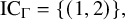 $$\begin{align*}\mathrm{IC}_\Gamma = \left\{(1,2)\right\},\end{align*}$$
and
 $(1,2)$
is the only cut edge in
$(1,2)$
is the only cut edge in
 $\Gamma $
that is not a leaf edge.
$\Gamma $
that is not a leaf edge.
For a connected graph
 $\Gamma $
on n vertices, we define
$\Gamma $
on n vertices, we define

where
 $G_s$
is defined as in Section 5 (i.e.,
$G_s$
is defined as in Section 5 (i.e.,
 $G_s$
is one of the two connected components of the graph
$G_s$
is one of the two connected components of the graph
 $([n],E(\Gamma )\setminus \{s\})$
). This formula is unaffected by a choice of component, as the sizes of the two connected components in
$([n],E(\Gamma )\setminus \{s\})$
). This formula is unaffected by a choice of component, as the sizes of the two connected components in
 $([n],E(\Gamma )\setminus \{s\})$
sum to n and
$([n],E(\Gamma )\setminus \{s\})$
sum to n and
 $\genfrac (){0pt}{0}{n}{\left | G_s \right |} = \genfrac (){0pt}{0}{n}{n-\left | G_s \right |}$
.
$\genfrac (){0pt}{0}{n}{\left | G_s \right |} = \genfrac (){0pt}{0}{n}{n-\left | G_s \right |}$
.
Remark 8.3. The invariant
 $D_\Gamma $
might be more concisely written as
$D_\Gamma $
might be more concisely written as
 $$\begin{align*}D_\Gamma = n-1 - \sum_{j \vdash \Gamma} \mathfrak{c}_\Gamma(j) + n\left(\left| \mathrm{LB}_\Gamma \right| + \left| \{B \in \mathrm{IB}_\Gamma \mid \left| B \right|> 2\} \right|\right) + \sum_{s \in \mathrm{IC}_\Gamma} \genfrac(){0pt}{0}{n}{\left| G_s \right|},\end{align*}$$
but the format in Equation 8.1 is more conducive to the proofs that follow.
Example 8.4. Consider the graph
 $\Gamma $
from Example 8.2 above. The three cut vertices are
$\Gamma $
from Example 8.2 above. The three cut vertices are
 $4$
,
$4$
,
 $1$
and
$1$
and
 $2$
. Each of those cut vertices separate
$2$
. Each of those cut vertices separate
 $\Gamma $
in to three connected components, so
$\Gamma $
in to three connected components, so
 $\mathfrak {c}_\Gamma (4) = \mathfrak {c}_\Gamma (1) = \mathfrak {c}_\Gamma (2) = 2$
. The block
$\mathfrak {c}_\Gamma (4) = \mathfrak {c}_\Gamma (1) = \mathfrak {c}_\Gamma (2) = 2$
. The block
 $B_3$
is the only block in
$B_3$
is the only block in
 $\mathrm {IB}_\Gamma $
with more than two vertices, so
$\mathrm {IB}_\Gamma $
with more than two vertices, so
 $\left | \{B \in \mathrm {IB}_\Gamma \mid \left | B \right |> 2\} \right | = 1$
. The only internal cut edge is
$\left | \{B \in \mathrm {IB}_\Gamma \mid \left | B \right |> 2\} \right | = 1$
. The only internal cut edge is
 $(1,2)$
, and this cut edge separates
$(1,2)$
, and this cut edge separates
 $\Gamma $
in to a component of size
$\Gamma $
in to a component of size
 $8$
and a component of size
$8$
and a component of size
 $4$
. We choose the component with vertex set
$4$
. We choose the component with vertex set
 $\{1,4,6,7,9,10,11,12\}$
, but note that
$\{1,4,6,7,9,10,11,12\}$
, but note that
 $\genfrac (){0pt}{0}{12}{8} = \genfrac (){0pt}{0}{12}{12-8} = \genfrac (){0pt}{0}{12}{4}$
. We compute that
$\genfrac (){0pt}{0}{12}{8} = \genfrac (){0pt}{0}{12}{12-8} = \genfrac (){0pt}{0}{12}{4}$
. We compute that
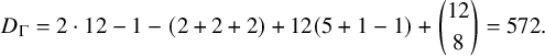 $$\begin{align*}D_\Gamma = 2\cdot 12-1 - \left(2+2+2\right) +12\left(5+1-1\right) + \genfrac(){0pt}{0}{12}{8} = 572. \end{align*}$$
Since
 $D_\Gamma $
is defined using only the block-cut tree, cut edges and cut vertices of
$D_\Gamma $
is defined using only the block-cut tree, cut edges and cut vertices of
 $\Gamma $
, it is an invariant of the isomorphism class of
$\Gamma $
, it is an invariant of the isomorphism class of
 $\Gamma $
. We note that if
$\Gamma $
. We note that if
 $\Gamma $
is
$\Gamma $
is
 $2$
-connected, it follows that
$2$
-connected, it follows that
 $D_\Gamma = 2n-1$
.
$D_\Gamma = 2n-1$
.
Lemma 8.5 below gives a formulation of
 $D_\Gamma $
specific to naturally labeled graphs. Its proof constructs important bijections that will be used later in the proofs of Proposition 8.9 and Corollary 9.3.
$D_\Gamma $
specific to naturally labeled graphs. Its proof constructs important bijections that will be used later in the proofs of Proposition 8.9 and Corollary 9.3.
Lemma 8.5. Let
 $\Gamma $
be a naturally labeled graph. Then
$\Gamma $
be a naturally labeled graph. Then
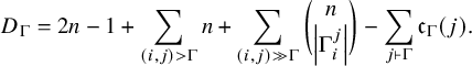 $$\begin{align*}D_\Gamma = 2n-1 + \sum_{(i,j)>\Gamma} n + \sum_{(i,j) \gg \Gamma} \genfrac(){0pt}{0}{n}{\left| \Gamma_i^j \right|} - \sum_{j \vdash \Gamma} \mathfrak{c}_\Gamma(j). \end{align*}$$
Proof. We compare the right-hand side of the formula above with (8.1). The clear cancellation between the two sides of the claimed equality is
 $2n-1-\sum\limits _{j \vdash \Gamma } \mathfrak {c}_\Gamma (j)$
. Thus, the claim will follow if
$2n-1-\sum\limits _{j \vdash \Gamma } \mathfrak {c}_\Gamma (j)$
. Thus, the claim will follow if
 $$ \begin{align} n\left(\left| \mathrm{LB}_\Gamma \right| + \left| \{B \in \mathrm{IB}_\Gamma \mid \left| B \right|> 2\} \right| - 1\right) + \sum_{s \in \mathrm{IC}_\Gamma} \genfrac(){0pt}{0}{n}{\left| G_s \right|}= \sum_{(i,j)>\Gamma} n + \sum_{(i,j) \gg \Gamma} \genfrac(){0pt}{0}{n}{\left| \Gamma_i^j \right|} . \end{align} $$
Since
 $\Gamma $
is naturally labeled, the block containing n is a leaf in the block-cut tree. So
$\Gamma $
is naturally labeled, the block containing n is a leaf in the block-cut tree. So
 $\left | \mathrm {LB}_\Gamma \right | - 1$
can be interpreted as the number of leaf blocks that do not contain n.
$\left | \mathrm {LB}_\Gamma \right | - 1$
can be interpreted as the number of leaf blocks that do not contain n.
In the remainder of the proof, we pair blocks in
 $\mathrm {LB}_\Gamma $
and
$\mathrm {LB}_\Gamma $
and
 $\mathrm {IB}_\Gamma $
that contribute on the left side of the claimed equality (*) with dominant pairs
$\mathrm {IB}_\Gamma $
that contribute on the left side of the claimed equality (*) with dominant pairs
 $(i,j)$
that contribute to the right side, in order to identify cancellations. The pairings that we will prove and use are as follows:
$(i,j)$
that contribute to the right side, in order to identify cancellations. The pairings that we will prove and use are as follows:
-
1. Leaf blocks
$B \in \mathrm {LB}_\Gamma $
with
$\left | B \right | = 2$
and
$n \notin B$
contribute n to the left side of (*) and are in bijection with strongly dominant pairs
$(i,j)$
where
$\left | \Gamma _i^j \right | = 1$
, which contribute
$\genfrac (){0pt}{0}{n}{1} = n$
to the right side. -
2. The set of internal cut edges
$\mathrm {IC}_\Gamma $
is equal to the set of strongly dominant pairs
$(i,j)$
such that
$\left | \Gamma _i^j \right |>1$
, and they both contribute
$\genfrac (){0pt}{0}{n}{\left | G_s \right |} = \genfrac (){0pt}{0}{n}{\left | \Gamma _i^j \right |}$
. -
3. Leaf blocks and internal blocks of size at least three (i.e., all blocks of size at least
$3$
) that do not contain the vertex n contribute n to the left side of the claimed equality and are in bijection with weakly dominant pairs
$(i,j)$
, each of which contributes n to the right side.


This list also serves as an outline of the proof that follows.
(1) Let B be a leaf block of size
 $2$
with vertex set
$2$
with vertex set
 $V(B) = \{i,j\}$
where
$V(B) = \{i,j\}$
where
 $i<j$
. Then the single edge
$i<j$
. Then the single edge
 $(i,j)$
within B is a cut edge of
$(i,j)$
within B is a cut edge of
 $\Gamma $
, and since B is a leaf block, that cut edge
$\Gamma $
, and since B is a leaf block, that cut edge
 $(i,j)$
must separate a single vertex. If this block does not contain n (so
$(i,j)$
must separate a single vertex. If this block does not contain n (so
 $j \neq n$
), then since
$j \neq n$
), then since
 $\Gamma $
is naturally labeled, the cut edge must be a dominant pair and that separated vertex must be i. So
$\Gamma $
is naturally labeled, the cut edge must be a dominant pair and that separated vertex must be i. So
 $(i,j) \gg \Gamma $
and
$(i,j) \gg \Gamma $
and
 $V(\Gamma _i^j) = \{i\}$
, and
$V(\Gamma _i^j) = \{i\}$
, and
 $\left | \Gamma _i^j \right | = 1$
. However, if
$\left | \Gamma _i^j \right | = 1$
. However, if
 $(i,j) \gg \Gamma $
and
$(i,j) \gg \Gamma $
and
 $\left | \Gamma _i^j \right | = 1$
, then i must be a leaf, and the subgraph
$\left | \Gamma _i^j \right | = 1$
, then i must be a leaf, and the subgraph
 $(\{i,j\},\{(i,j)\})$
is a block in
$(\{i,j\},\{(i,j)\})$
is a block in
 $\Gamma $
that does not contain n. In particular, we have shown
$\Gamma $
that does not contain n. In particular, we have shown
 $$\begin{align*}\{B \in \mathrm{LB}_\Gamma \mid \left| B \right| = 2,\; n \notin B\} = \{B \in \mathrm{LB}_\Gamma \mid V(B) = \{i,j\},\; (i,j) \gg \Gamma\}.\end{align*}$$
So the leaf blocks B in
 $\Gamma $
of size
$\Gamma $
of size
 $2$
are in natural bijection with the dominant pairs
$2$
are in natural bijection with the dominant pairs
 $(i,j) \gg \Gamma $
where
$(i,j) \gg \Gamma $
where
 $\left | \Gamma _i^j \right | = 1$
. Formally,
$\left | \Gamma _i^j \right | = 1$
. Formally,
 $\left | \{B \in \mathrm {LB}_\Gamma \mid \left | B \right | = 2,\; n \notin B\} \right | = \left | \left \{(i,j) \gg \Gamma \mid \left | \Gamma _i^j \right | = 1\right \} \right |$
. Thus,
$\left | \{B \in \mathrm {LB}_\Gamma \mid \left | B \right | = 2,\; n \notin B\} \right | = \left | \left \{(i,j) \gg \Gamma \mid \left | \Gamma _i^j \right | = 1\right \} \right |$
. Thus,
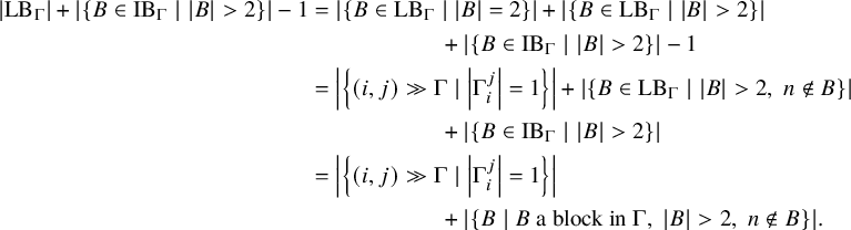 $$ \begin{align*} \left| \mathrm{LB}_\Gamma \right| + \left| \{B \in \mathrm{IB}_\Gamma \mid \left| B \right|> 2\} \right| - 1 &= \left| \{B \in \mathrm{LB}_\Gamma \mid \left| B \right| = 2\} \right|+\left| \{B \in \mathrm{LB}_\Gamma \mid \left| B \right| > 2\} \right| \\&\hspace{2cm}+ \left| \{B \in \mathrm{IB}_\Gamma \mid \left| B \right| > 2\} \right| - 1 \\ &= \left| \left\{(i,j) \gg \Gamma \mid \left| \Gamma_i^j \right| = 1\right\} \right|+\left| \{B \in \mathrm{LB}_\Gamma \mid \left| B \right| > 2,\; n \notin B\} \right| \\&\hspace{2cm}+ \left| \{B \in \mathrm{IB}_\Gamma \mid \left| B \right| > 2\} \right| \\ &= \left| \left\{(i,j) \gg \Gamma \mid \left| \Gamma_i^j \right|=1\right\} \right| \\&\hspace{2cm}+ \left| \{B \mid B \text{ a block in }\Gamma,\; \left| B \right| > 2,\; n \notin B\} \right|. \end{align*} $$
We cancel
 ${ n\left | \left \{(i,j) \gg \Gamma \mid \left | \Gamma _i^j \right |=1\right \} \right |}$
from the left side and
${ n\left | \left \{(i,j) \gg \Gamma \mid \left | \Gamma _i^j \right |=1\right \} \right |}$
from the left side and
 ${ \sum\limits _{\substack {(i,j) \gg \Gamma \\ \left | \Gamma _i^j \right |=1}} \genfrac (){0pt}{0}{n}{1}}$
from the right side of (*), and it remains to prove that
${ \sum\limits _{\substack {(i,j) \gg \Gamma \\ \left | \Gamma _i^j \right |=1}} \genfrac (){0pt}{0}{n}{1}}$
from the right side of (*), and it remains to prove that
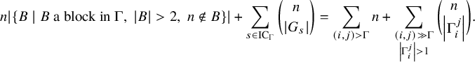 $$ \begin{align} n\left| \{B \mid B \text{ a block in }\Gamma,\; \left| B \right|> 2,\; n \notin B\} \right| + \sum_{s \in \mathrm{IC}_\Gamma} \genfrac(){0pt}{0}{n}{\left| G_s \right|}= \sum_{(i,j)>\Gamma} n + \sum_{\substack{(i,j) \gg \Gamma \\ \left| \Gamma_i^j \right|>1 }} \genfrac(){0pt}{0}{n}{\left| \Gamma_i^j \right|}. \end{align} $$
(2) Now if
 $s = (i,j) \in \mathrm {IC}_\Gamma $
, then s is a cut edge, and since
$s = (i,j) \in \mathrm {IC}_\Gamma $
, then s is a cut edge, and since
 $\Gamma $
is naturally labeled,
$\Gamma $
is naturally labeled,
 $n \notin \{i,j\}$
. So if
$n \notin \{i,j\}$
. So if
 $(i,j) \in \mathrm {IC}_\Gamma $
, then
$(i,j) \in \mathrm {IC}_\Gamma $
, then
 $(i,j) \gg \Gamma $
and
$(i,j) \gg \Gamma $
and
 $\left | \Gamma _i^j \right |> 1$
; otherwise, i is a leaf and the block B where
$\left | \Gamma _i^j \right |> 1$
; otherwise, i is a leaf and the block B where
 $V(B) = \{i,j\}$
is not an internal block. However, if
$V(B) = \{i,j\}$
is not an internal block. However, if
 $(i,j) \gg \Gamma $
and
$(i,j) \gg \Gamma $
and
 $\left | \Gamma _i^j \right |> 1$
, then i cannot be a leaf,
$\left | \Gamma _i^j \right |> 1$
, then i cannot be a leaf,
 $(i,j)$
must be a cut edge and the block B where
$(i,j)$
must be a cut edge and the block B where
 $V(B) = \{i,j\}$
is not a leaf in the block-cut tree. So
$V(B) = \{i,j\}$
is not a leaf in the block-cut tree. So
 $\mathrm {IC}_\Gamma = \left \{(i,j) \gg \Gamma \mid \left | \Gamma _i^j \right |> 1\right \}$
. In particular,
$\mathrm {IC}_\Gamma = \left \{(i,j) \gg \Gamma \mid \left | \Gamma _i^j \right |> 1\right \}$
. In particular,
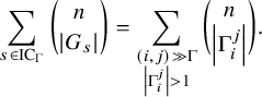 $$\begin{align*}\sum_{s \in \mathrm{IC}_\Gamma} \genfrac(){0pt}{0}{n}{\left| G_s \right|} = \sum_{\substack{(i,j) \gg \Gamma\\ \left| \Gamma_i^j \right|> 1}} \genfrac(){0pt}{0}{n}{\left| \Gamma_i^j \right|}. \end{align*}$$
After cancelling this value from both sides of (**), it remains to show that
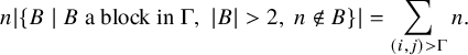 $$ \begin{align} n\left| \{B \mid B \text{ a block in }\Gamma,\; \left| B \right|> 2,\; n \notin B\} \right| = \sum_{(i,j)>\Gamma} n. \end{align} $$
(3) We argue that
 $$\begin{align*}\left| \{B \mid B \text{ a block in }\Gamma,\; \left| B \right|> 2,\; n \notin B\} \right| = \left| \{(i,j) > \Gamma\} \right|.\end{align*}$$
The bijection is as follows. If B is a block in
 $\Gamma $
that does not contain n, then there is a unique path from B to the block
$\Gamma $
that does not contain n, then there is a unique path from B to the block
 $B_0$
that contains n in the block-cut tree of
$B_0$
that contains n in the block-cut tree of
 $\Gamma $
. The first edge in that path is from B to a cut vertex of
$\Gamma $
. The first edge in that path is from B to a cut vertex of
 $\Gamma $
that is contained within B. Let j be this cut vertex, and let i be the maximal vertex in B that is not equal to j. Note that B is not connected to n in
$\Gamma $
that is contained within B. Let j be this cut vertex, and let i be the maximal vertex in B that is not equal to j. Note that B is not connected to n in
 $\Gamma - j$
.
$\Gamma - j$
.
Since
 $\Gamma $
is naturally labeled,
$\Gamma $
is naturally labeled,
 $(i,j)$
is an edge and i must also be the maximal vertex in its connected component of
$(i,j)$
is an edge and i must also be the maximal vertex in its connected component of
 $\Gamma - j$
(every path from n to that component first passes through j, and i is the largest vertex in that component that is adjacent to j). Since
$\Gamma - j$
(every path from n to that component first passes through j, and i is the largest vertex in that component that is adjacent to j). Since
 $\left | B \right |> 2$
, there is at least one other element of B in the neighborhood of j, so
$\left | B \right |> 2$
, there is at least one other element of B in the neighborhood of j, so
 $(i,j)$
is not a cut edge. In particular,
$(i,j)$
is not a cut edge. In particular,
 $(i,j)> \Gamma $
.
$(i,j)> \Gamma $
.
However, if
 $(i,j)> \Gamma $
, let B be the block containing i. This block cannot contain n by the definition of a natural label and must be of size at least
$(i,j)> \Gamma $
, let B be the block containing i. This block cannot contain n by the definition of a natural label and must be of size at least
 $2$
since
$2$
since
 $(i,j)$
is not a cut edge.
$(i,j)$
is not a cut edge.
So we have a bijection, proving as a consequence (***), and the claim follows.
The bijection between certain dominant pairs and blocks that we constructed in the proof of Lemma 8.5 above will be used again to compute a recursive formula for
 $D_\Gamma $
and provide a label-independent formula for
$D_\Gamma $
and provide a label-independent formula for
 $\mathbf {ch}\left (\mathrm {L}_{\Gamma }\right )_1$
and
$\mathbf {ch}\left (\mathrm {L}_{\Gamma }\right )_1$
and
 $\mathbf {ch}\left (\mathrm {R}_{\Gamma }\right )_1$
in Corollary 9.3 below. Visually, when
$\mathbf {ch}\left (\mathrm {R}_{\Gamma }\right )_1$
in Corollary 9.3 below. Visually, when
 $\Gamma $
is naturally labeled, we have the following correspondences between blocks in
$\Gamma $
is naturally labeled, we have the following correspondences between blocks in
 $\Gamma $
and dominant pairs.
$\Gamma $
and dominant pairs.
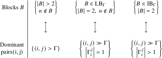
Example 8.6. Consider the naturally labeled graph
 $\Gamma $
drawn below:
$\Gamma $
drawn below:
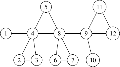
with block-cut tree
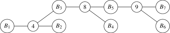
The blocks of size at least
 $2$
that do not contain n correspond to weakly dominant pairs in the following manner:
$2$
that do not contain n correspond to weakly dominant pairs in the following manner:
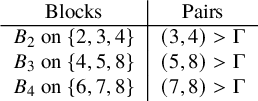
The leaf blocks of size
 $2$
that do not contain n correspond to strongly dominant pairs
$2$
that do not contain n correspond to strongly dominant pairs
 $(i,j)$
where
$(i,j)$
where
 $\left | \Gamma _i^j \right | = 1$
in the following manner:
$\left | \Gamma _i^j \right | = 1$
in the following manner:
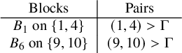
Finally, the internal block
 $B_5$
on
$B_5$
on
 $\{8,9\}$
(so of size
$\{8,9\}$
(so of size
 $2$
) corresponds to the dominant pair
$2$
) corresponds to the dominant pair
 $(8,9) \gg \Gamma $
.
$(8,9) \gg \Gamma $
.
Example 8.7. When
 $\Gamma $
is naturally labeled, each sum appearing in the formula in Lemma 8.5 has the following combinatorial interpretation:
$\Gamma $
is naturally labeled, each sum appearing in the formula in Lemma 8.5 has the following combinatorial interpretation:
-
•
$n\;$
: Every vertex of
$\Gamma $
contributes
$1$
to the sum, -
•
${ n-1-\sum\limits _{j \vdash \Gamma } \mathfrak {c}_\Gamma (j)}\;$
: Every vertex that is not the lower vertex in a dominant pair or the vertex n contributes an additional
$1$
to the sum (recall that the lower vertices in a dominant pair determine the pair uniquely). -
•
${ \sum\limits _{j \vdash \Gamma } \sum\limits _{(i,j)>\Gamma } n }\;$
: Every weakly dominant pair contributes n to the sum. -
•
${ \sum\limits _{j \vdash \Gamma } \sum\limits _{(i,j)\gg \Gamma } \genfrac (){0pt}{0}{n}{\left | \Gamma _i^j \right |}}\;$
: Every strongly dominant pair
$(i,j)$
contributes
$\genfrac (){0pt}{0}{n}{\left | \Gamma _i^j \right |}$
to the sum.


Below, we have drawn
 $\Gamma $
from Example 6.11, with the associated values for
$\Gamma $
from Example 6.11, with the associated values for
 $D_\Gamma $
in blue. In this picture, dashed lines indicate weak dominance and double lines indicate strong dominance.
$D_\Gamma $
in blue. In this picture, dashed lines indicate weak dominance and double lines indicate strong dominance.
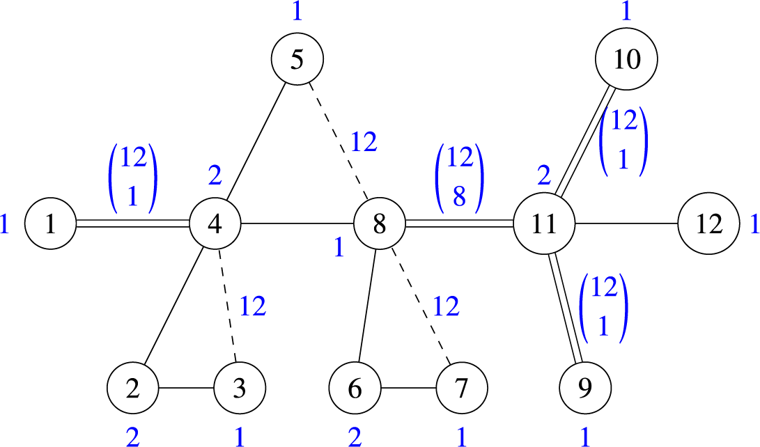
Remark 8.8. It is not obvious that the formula in Lemma 8.5 is the same for different naturally labeled graphs in the isomorphism class. However, it is clear from the definition in (8.1) that
 $D_\Gamma $
is an invariant, so they must be equal.
$D_\Gamma $
is an invariant, so they must be equal.
The following Proposition 8.9 gives an inductive formula for
 $D_\Gamma $
when
$D_\Gamma $
when
 $\Gamma $
is cliqued and naturally labeled that matches the inductive formula for
$\Gamma $
is cliqued and naturally labeled that matches the inductive formula for
 $\dim _{\mathbb {C}}(\mathcal {M}_{\Gamma }^1)$
from Theorem 7.2.
$\dim _{\mathbb {C}}(\mathcal {M}_{\Gamma }^1)$
from Theorem 7.2.
Proposition 8.9. If
 $\Gamma $
is a cliqued and naturally labeled graph on at least
$\Gamma $
is a cliqued and naturally labeled graph on at least
 $4$
vertices, then
$4$
vertices, then
 $D_\Gamma $
can be computed recursively as follows:
$D_\Gamma $
can be computed recursively as follows:
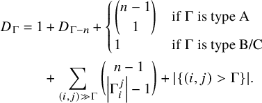 $$ \begin{align*} D_\Gamma = 1&+D_{\Gamma-n} + \begin{cases} \genfrac(){0pt}{0}{n-1}{1} &\text{if } \Gamma \; \text{is type A} \\ 1 &\text{if }\Gamma \; \text{is type B/C} \end{cases} \\&+ \sum_{(i,j) \gg \Gamma} \genfrac(){0pt}{0}{n-1}{\left| \Gamma_i^j \right|-1} + \left| \left\{(i,j)> \Gamma \right\} \right|. \end{align*} $$
Before proving Proposition 8.9, we prove several computational lemmas and construct a finer categorization of type A graphs. The key idea is to concretely describe the block-cut tree of
 $\Gamma - n$
in terms of the block-cut tree of
$\Gamma - n$
in terms of the block-cut tree of
 $\Gamma $
.
$\Gamma $
.
If B is a block in
 $\Gamma $
that does not contain n, then B is still
$\Gamma $
that does not contain n, then B is still
 $2$
-connected in
$2$
-connected in
 $\Gamma - n$
. Additionally, if i and k where
$\Gamma - n$
. Additionally, if i and k where
 $n \notin \{i,k\}$
are vertices in
$n \notin \{i,k\}$
are vertices in
 $\Gamma $
such that i and k are in different connected components of
$\Gamma $
such that i and k are in different connected components of
 $\Gamma - j$
, then i and k are also in different connected components of
$\Gamma - j$
, then i and k are also in different connected components of
 $ (\Gamma - n) - j$
. In particular, If B is a block in
$ (\Gamma - n) - j$
. In particular, If B is a block in
 $\Gamma $
that does not contain n, then B is a block in
$\Gamma $
that does not contain n, then B is a block in
 $\Gamma - n$
.
$\Gamma - n$
.
Lemma 8.10 below describes the simplest case, when
 $\Gamma $
is either type B or type C
$\Gamma $
is either type B or type C
Lemma 8.10. Let
 $\Gamma $
be a cliqued and naturally labeled graph on at least
$\Gamma $
be a cliqued and naturally labeled graph on at least
 $4$
vertices. If
$4$
vertices. If
 $\Gamma $
is of type B or C, then the following equalities hold:
$\Gamma $
is of type B or C, then the following equalities hold:
-
•
$\left | \mathrm {LB}_\Gamma \right | = \left | \mathrm {LB}_{\Gamma - n} \right |$
, -
•
$\mathrm {IB}_\Gamma = \mathrm {IB}_{\Gamma - n}$
, and -
•
$\mathrm {IC}_\Gamma = \mathrm {IC}_{\Gamma -n}$
.


Proof. Let
 $B_0$
be the block in
$B_0$
be the block in
 $\Gamma $
that contains n. Since
$\Gamma $
that contains n. Since
 $\Gamma $
is type B or C,
$\Gamma $
is type B or C,
 $\left | B_0 \right |> 2$
. Since
$\left | B_0 \right |> 2$
. Since
 $\Gamma $
is cliqued, the subgraph
$\Gamma $
is cliqued, the subgraph
 $B_0 -n$
has at least
$B_0 -n$
has at least
 $2$
vertices and is also a clique, and in particular,
$2$
vertices and is also a clique, and in particular,
 $B_0 - n$
is a block in
$B_0 - n$
is a block in
 $\Gamma - n$
. Every other block or cut vertex in
$\Gamma - n$
. Every other block or cut vertex in
 $\Gamma $
is a block or cut vertex in
$\Gamma $
is a block or cut vertex in
 $\Gamma - n$
. Thus, the block-cut tree of
$\Gamma - n$
. Thus, the block-cut tree of
 $\Gamma $
is isomorphic to the block-cut tree of
$\Gamma $
is isomorphic to the block-cut tree of
 $\Gamma - n$
.
$\Gamma - n$
.
Since the block-cut trees are isomorphic they have the same number of leaves, and so
 $\left | \mathrm {LB}_\Gamma \right | = \left | \mathrm {LB}_{\Gamma - n} \right |$
. Since the only block that changes is
$\left | \mathrm {LB}_\Gamma \right | = \left | \mathrm {LB}_{\Gamma - n} \right |$
. Since the only block that changes is
 $B_0$
and all non-leaf blocks in
$B_0$
and all non-leaf blocks in
 $\Gamma $
are non-leaf blocks in
$\Gamma $
are non-leaf blocks in
 $\Gamma - n$
, it follows that
$\Gamma - n$
, it follows that
 $\mathrm {IB}_\Gamma = \mathrm {IB}_{\Gamma - n}$
. This equality implies
$\mathrm {IB}_\Gamma = \mathrm {IB}_{\Gamma - n}$
. This equality implies
 $\mathrm {IC}_\Gamma = \mathrm {IC}_{\Gamma -n}$
by definition.
$\mathrm {IC}_\Gamma = \mathrm {IC}_{\Gamma -n}$
by definition.
We now assume that
 $\Gamma $
is type A. We will give a similar computation for type-A graphs, but there are several cases to consider. Since
$\Gamma $
is type A. We will give a similar computation for type-A graphs, but there are several cases to consider. Since
 $(n-1,n)$
is a cut edge, it corresponds to a block
$(n-1,n)$
is a cut edge, it corresponds to a block
 $B_0$
containing
$B_0$
containing
 $ n$
in
$ n$
in
 $\Gamma $
that has no natural counterpart in the block-cut tree of
$\Gamma $
that has no natural counterpart in the block-cut tree of
 $\Gamma - n$
. Not only that, but
$\Gamma - n$
. Not only that, but
 $n-1$
may not be a cut vertex in
$n-1$
may not be a cut vertex in
 $\Gamma -n$
.
$\Gamma -n$
.
Addressing this requires further decomposition of type A graphs, which we denote A1, A2, A3, A4 and A5. We will define them carefully below, but the consequences in each case in terms of moving from the block-cut tree of
 $\Gamma $
to that of
$\Gamma $
to that of
 $\Gamma - n$
are essentially as follows (recall
$\Gamma - n$
are essentially as follows (recall
 $B_0$
is the block in
$B_0$
is the block in
 $\Gamma $
containing n):
$\Gamma $
containing n):
-
(A1) The block-cut tree of
$\Gamma - n$
is simply that of
$\Gamma $
with the block
$B_0$
removed. -
(A2) The block-cut tree of
$\Gamma - n$
is the block-cut tree of
$\Gamma $
with the block
$B_0$
and the cut vertex
$n-1$
removed, and an internal block
$B'$
of size
$2$
for
$\Gamma $
becomes a leaf block for
$\Gamma -n$
. -
(A3) The block-cut tree of
$\Gamma - n$
is the block-cut tree of
$\Gamma $
with the block
$B_0$
and the cut vertex
$n-1$
removed, but every other internal (resp. leaf) block of
$\Gamma $
remains an internal (resp. leaf) block of
$\Gamma - n$
. -
(A4) The block-cut tree of
$\Gamma - n$
is the block-cut tree of
$\Gamma $
with the block
$B_0$
and the cut vertex
$n-1$
removed, and an internal block
$B'$
of size greater than
$2$
for
$\Gamma $
becomes a leaf block for
$\Gamma - n$
. -
(A5) The graph
$\Gamma - n$
is
$2$
-connected.


First, a type A graph
 $\Gamma $
is type A1 if
$\Gamma $
is type A1 if
 $\mathfrak {c}_\Gamma (n-1)> 1$
. Graphically,
$\mathfrak {c}_\Gamma (n-1)> 1$
. Graphically,
 $\Gamma $
looks like
$\Gamma $
looks like
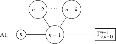
Note that in type A1,
 $\Gamma - n$
has the same cut vertices as
$\Gamma - n$
has the same cut vertices as
 $\Gamma $
, so the block-cut tree of
$\Gamma $
, so the block-cut tree of
 $\Gamma - n$
is the block-cut tree of
$\Gamma - n$
is the block-cut tree of
 $\Gamma $
with
$\Gamma $
with
 $B_0$
removed.
$B_0$
removed.
If
 $\Gamma $
is type A but not type A1, then
$\Gamma $
is type A but not type A1, then
 $n-1$
is a cut vertex of
$n-1$
is a cut vertex of
 $\Gamma $
, but it is not a cut vertex of
$\Gamma $
, but it is not a cut vertex of
 $\Gamma - n$
. So the block-cut tree of
$\Gamma - n$
. So the block-cut tree of
 $\Gamma - n$
is the block-cut tree of
$\Gamma - n$
is the block-cut tree of
 $\Gamma $
with both the block
$\Gamma $
with both the block
 $B_0$
and the cut vertex
$B_0$
and the cut vertex
 $n-1$
removed. In particular,
$n-1$
removed. In particular,
 $n-1$
is contained within precisely two blocks in
$n-1$
is contained within precisely two blocks in
 $\Gamma $
: one that contains n (so
$\Gamma $
: one that contains n (so
 $B_0$
) and one that contains
$B_0$
) and one that contains
 $n-2$
. Let
$n-2$
. Let
 $B'$
be the block in
$B'$
be the block in
 $\Gamma $
that contains
$\Gamma $
that contains
 $n-1$
and
$n-1$
and
 $n-2$
.
$n-2$
.
We say
 $\Gamma $
is type A2 if
$\Gamma $
is type A2 if
 $\left | B' \right | = 2$
(i.e.,
$\left | B' \right | = 2$
(i.e.,
 $V(B') = \{n-2,n-1\}$
). Graphically,
$V(B') = \{n-2,n-1\}$
). Graphically,
 $\Gamma $
and its block-cut tree look like
$\Gamma $
and its block-cut tree look like
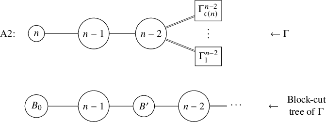
Note that the
 $B'$
where
$B'$
where
 $V(B') = \{n-2,n-1\}$
is associated to an internal cut edge in
$V(B') = \{n-2,n-1\}$
is associated to an internal cut edge in
 $\Gamma $
and is a leaf block in
$\Gamma $
and is a leaf block in
 $\Gamma - n$
.
$\Gamma - n$
.
The graph
 $\Gamma $
is type A3 if
$\Gamma $
is type A3 if
 $\left | B' \right |> 2$
and
$\left | B' \right |> 2$
and
 $B'$
contains more than
$B'$
contains more than
 $2$
cut vertices of
$2$
cut vertices of
 $\Gamma $
. So
$\Gamma $
. So
 $B'$
is adjacent to more than two vertices in the block-cut tree of
$B'$
is adjacent to more than two vertices in the block-cut tree of
 $\Gamma $
. Graphically, the block-cut tree of
$\Gamma $
. Graphically, the block-cut tree of
 $\Gamma $
looks like
$\Gamma $
looks like
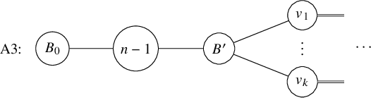
where
 $k> 1$
. Note that
$k> 1$
. Note that
 $B'$
is an internal block in both
$B'$
is an internal block in both
 $\Gamma $
and
$\Gamma $
and
 $\Gamma - n$
.
$\Gamma - n$
.
The graph
 $\Gamma $
is type A4 if
$\Gamma $
is type A4 if
 $\left | B' \right |> 2$
, and
$\left | B' \right |> 2$
, and
 $B'$
contains precisely
$B'$
contains precisely
 $2$
cut vertices of
$2$
cut vertices of
 $\Gamma $
,
$\Gamma $
,
 $n-1$
and some other cut vertex v of
$n-1$
and some other cut vertex v of
 $\Gamma $
. In particular,
$\Gamma $
. In particular,
 $B'$
is adjacent to precisely two vertices in the block-cut tree of
$B'$
is adjacent to precisely two vertices in the block-cut tree of
 $\Gamma $
. Graphically, the block-cut tree of
$\Gamma $
. Graphically, the block-cut tree of
 $\Gamma $
looks like
$\Gamma $
looks like
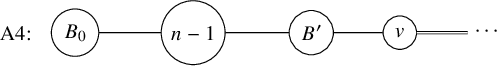
Note that
 $B'$
is an internal block of size at least
$B'$
is an internal block of size at least
 $3$
in
$3$
in
 $\Gamma $
and a leaf block in
$\Gamma $
and a leaf block in
 $\Gamma - n$
.
$\Gamma - n$
.
Finally, the graph
 $\Gamma $
is type A5 if
$\Gamma $
is type A5 if
 $n-1$
is the only cut vertex in
$n-1$
is the only cut vertex in
 $B'$
. In particular,
$B'$
. In particular,
 $B_0$
and
$B_0$
and
 $B'$
are the only two blocks in
$B'$
are the only two blocks in
 $\Gamma $
, so the block-cut tree of
$\Gamma $
, so the block-cut tree of
 $\Gamma $
is
$\Gamma $
is
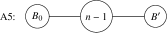
The computations for type A5 are generally easy, as
 $\Gamma - n$
is
$\Gamma - n$
is
 $2$
-connected.
$2$
-connected.
Lemmas 8.11, 8.12 and 8.13 below use this finer categorization of type A graphs to explicitly compute the relationship between sums in the formulas of
 $D_\Gamma $
and
$D_\Gamma $
and
 $D_{\Gamma -n}$
. For the proofs of Lemmas 8.12, 8.13 and 8.11 below,
$D_{\Gamma -n}$
. For the proofs of Lemmas 8.12, 8.13 and 8.11 below,
 $B_0$
is the block in
$B_0$
is the block in
 $\Gamma $
that contains n and (if
$\Gamma $
that contains n and (if
 $\Gamma $
type A2-A5)
$\Gamma $
type A2-A5)
 $B'$
is the block in
$B'$
is the block in
 $\Gamma $
that contains
$\Gamma $
that contains
 $n-1$
but not n (so
$n-1$
but not n (so
 $B'$
is still a block in
$B'$
is still a block in
 $\Gamma - n$
).
$\Gamma - n$
).
Lemma 8.11. Let
 $\Gamma $
be a cliqued and naturally labeled graph on at least
$\Gamma $
be a cliqued and naturally labeled graph on at least
 $4$
vertices. Then the number of leaf blocks in
$4$
vertices. Then the number of leaf blocks in
 $\Gamma - n$
is
$\Gamma - n$
is
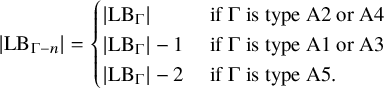 $$\begin{align*}\left| \mathrm{LB}_{\Gamma - n} \right| = \begin{cases} \left| \mathrm{LB}_{\Gamma} \right| & \text{ if } \Gamma \text{ is type A2 or A4} \\ \left| \mathrm{LB}_{\Gamma} \right|-1 & \text{ if } \Gamma \text{ is type A1 or A3} \\ \left| \mathrm{LB}_{\Gamma} \right|-2 & \text{ if } \Gamma \text{ is type A5.} \end{cases}\end{align*}$$
Proof. If
 $\Gamma $
is type A2 or A4, then
$\Gamma $
is type A2 or A4, then
 $B' \in \mathrm {LB}_{\Gamma -n}$
is a leaf block of
$B' \in \mathrm {LB}_{\Gamma -n}$
is a leaf block of
 $\Gamma -n$
, but
$\Gamma -n$
, but
 $B' \in \mathrm {IB}_\Gamma $
is an internal block of
$B' \in \mathrm {IB}_\Gamma $
is an internal block of
 $\Gamma $
. So
$\Gamma $
. So
 $\mathrm {LB}_{\Gamma -n} = \left (\mathrm {LB}_{\Gamma } \setminus \{B_0\}\right ) \cup \{B'\}$
. Less formally, we lose a block
$\mathrm {LB}_{\Gamma -n} = \left (\mathrm {LB}_{\Gamma } \setminus \{B_0\}\right ) \cup \{B'\}$
. Less formally, we lose a block
 $B_0$
and gain a block
$B_0$
and gain a block
 $B'$
, maintaining the same size.
$B'$
, maintaining the same size.
If
 $\Gamma $
is type
$\Gamma $
is type
 $A1$
or
$A1$
or
 $A3$
, every leaf block in
$A3$
, every leaf block in
 $\Gamma - n$
is a leaf block in
$\Gamma - n$
is a leaf block in
 $\Gamma $
, but we still lose
$\Gamma $
, but we still lose
 $B_0$
. So the size decrements by
$B_0$
. So the size decrements by
 $1$
.
$1$
.
If
 $\Gamma $
is type A5, then
$\Gamma $
is type A5, then
 $\Gamma $
has two leaf blocks (
$\Gamma $
has two leaf blocks (
 $B_0 $
and
$B_0 $
and
 $B'$
), whereas
$B'$
), whereas
 $\Gamma - n$
is a clique, with zero leaf blocks. We directly compute
$\Gamma - n$
is a clique, with zero leaf blocks. We directly compute
 $\left | \mathrm {LB}_{\Gamma } \right | = 2$
and
$\left | \mathrm {LB}_{\Gamma } \right | = 2$
and
 $\left | \mathrm {LB}_{\Gamma -n} \right | = 0$
.
$\left | \mathrm {LB}_{\Gamma -n} \right | = 0$
.
Lemma 8.12. Let
 $\Gamma $
be a cliqued and naturally labeled graph on at least
$\Gamma $
be a cliqued and naturally labeled graph on at least
 $4$
vertices. Then
$4$
vertices. Then
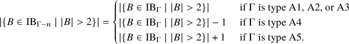 $$\begin{align*}\left| \{B \in \mathrm{IB}_{\Gamma-n} \mid \left| B \right|> 2\} \right| = \begin{cases} \left| \{B \in \mathrm{IB}_\Gamma \mid \left| B \right| > 2\} \right| & \text{ if } \Gamma \text{ is type A1, A2, or A3} \\ \left| \{B \in \mathrm{IB}_\Gamma \mid \left| B \right| > 2\} \right|-1 & \text{ if } \Gamma \text{ is type A4} \\ \left| \{B \in \mathrm{IB}_\Gamma \mid \left| B \right| > 2\} \right|+1 & \text{ if } \Gamma \text{ is type A5.} \end{cases}\end{align*}$$
Proof. If
 $\Gamma $
is type A1, then every internal block of
$\Gamma $
is type A1, then every internal block of
 $\Gamma $
is an internal block of
$\Gamma $
is an internal block of
 $\Gamma '$
and vice versa. If
$\Gamma '$
and vice versa. If
 $\Gamma $
is type A2, then
$\Gamma $
is type A2, then
 $B'$
where
$B'$
where
 $V(B') = \{n-2,n-1\}$
is an internal block for
$V(B') = \{n-2,n-1\}$
is an internal block for
 $\Gamma $
but a leaf block for
$\Gamma $
but a leaf block for
 $\Gamma - n$
. However,
$\Gamma - n$
. However,
 $B'$
is not counted above since
$B'$
is not counted above since
 $\left | B' \right | = 2$
. Every other internal block of
$\left | B' \right | = 2$
. Every other internal block of
 $\Gamma $
is an internal block of
$\Gamma $
is an internal block of
 $\Gamma - n$
and vice versa. If
$\Gamma - n$
and vice versa. If
 $\Gamma $
is type A3, then
$\Gamma $
is type A3, then
 $B'$
is still an internal block in
$B'$
is still an internal block in
 $\Gamma - n$
because it is adjacent to more than
$\Gamma - n$
because it is adjacent to more than
 $2$
cut vertices in the block-cut tree of
$2$
cut vertices in the block-cut tree of
 $\Gamma - n$
. Every other internal block is also the same, and so the equality follows.
$\Gamma - n$
. Every other internal block is also the same, and so the equality follows.
If
 $\Gamma $
is type A4, then
$\Gamma $
is type A4, then
 $B'$
is an internal block of
$B'$
is an internal block of
 $\Gamma $
but a leaf block in
$\Gamma $
but a leaf block in
 $\Gamma - n$
. Every other internal block in
$\Gamma - n$
. Every other internal block in
 $\Gamma - n$
is an internal block in
$\Gamma - n$
is an internal block in
 $\Gamma $
, so
$\Gamma $
, so
 $\left | \{B \in \mathrm {IB}_{\Gamma -n} \mid \left | B \right |> 2\} \right | = \left | \{B \in \mathrm {IB}_\Gamma \mid \left | B \right | > 2\} \right |-1$
.
$\left | \{B \in \mathrm {IB}_{\Gamma -n} \mid \left | B \right |> 2\} \right | = \left | \{B \in \mathrm {IB}_\Gamma \mid \left | B \right | > 2\} \right |-1$
.
If
 $\Gamma $
is type A5, then
$\Gamma $
is type A5, then
 $\mathrm {IB}_\Gamma = \emptyset $
. However,
$\mathrm {IB}_\Gamma = \emptyset $
. However,
 $\mathrm {IB}_{\Gamma - n} = \{B'\}$
. Since
$\mathrm {IB}_{\Gamma - n} = \{B'\}$
. Since
 $\Gamma $
has at least
$\Gamma $
has at least
 $4$
vertices, we know that
$4$
vertices, we know that
 $\left | B' \right |> 2$
, and the claim follows.
$\left | B' \right |> 2$
, and the claim follows.
Lemma 8.13. Let
 $\Gamma $
be a cliqued and naturally labeled graph on at least
$\Gamma $
be a cliqued and naturally labeled graph on at least
 $4$
vertices. Then the internal cut edges in
$4$
vertices. Then the internal cut edges in
 $\Gamma -n$
are
$\Gamma -n$
are
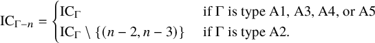 $$\begin{align*}\mathrm{IC}_{\Gamma-n} = \begin{cases} \mathrm{IC}_\Gamma & \text{ if } \Gamma \text{ is type A1, A3, A4, or A5} \\ \mathrm{IC}_\Gamma \setminus \{(n-2,n-3)\} & \text{ if } \Gamma \text{ is type A2.} \end{cases}\end{align*}$$
Proof. The set
 $\mathrm {IC}_\Gamma $
is the set of internal cut edges in
$\mathrm {IC}_\Gamma $
is the set of internal cut edges in
 $\Gamma $
. The two types where
$\Gamma $
. The two types where
 $B'$
is an internal block in
$B'$
is an internal block in
 $\Gamma $
but a leaf block in
$\Gamma $
but a leaf block in
 $\Gamma - n$
are types A2, A3 and A4. In types A3 and A4, the block
$\Gamma - n$
are types A2, A3 and A4. In types A3 and A4, the block
 $B'$
is assumed to have size
$B'$
is assumed to have size
 $\left | B \right |> 2$
and so does not correspond to an element of
$\left | B \right |> 2$
and so does not correspond to an element of
 $\mathrm {IC}_\Gamma $
. If
$\mathrm {IC}_\Gamma $
. If
 $\Gamma $
is type A2,
$\Gamma $
is type A2,
 $B'$
contributes to
$B'$
contributes to
 $\mathrm {IC}_\Gamma $
but not
$\mathrm {IC}_\Gamma $
but not
 $\mathrm {IC}_{\Gamma - n}$
, and that contribution is precisely the cut edge
$\mathrm {IC}_{\Gamma - n}$
, and that contribution is precisely the cut edge
 $(n-2,n-1)$
.
$(n-2,n-1)$
.
Now we are ready to prove the recursive formula for
 $D_\Gamma $
.
$D_\Gamma $
.
Proof of Proposition 8.9.
Consider the sum
 $\sum\limits _{j \vdash \Gamma - n} \mathfrak {c}_{\Gamma - n}(j)$
. If
$\sum\limits _{j \vdash \Gamma - n} \mathfrak {c}_{\Gamma - n}(j)$
. If
 $\Gamma $
is type B or C, then every cut vertex of
$\Gamma $
is type B or C, then every cut vertex of
 $\Gamma $
is a cut vertex of
$\Gamma $
is a cut vertex of
 $\Gamma - n$
and vice versa. For each such cut vertex
$\Gamma - n$
and vice versa. For each such cut vertex
 $j \vdash \Gamma $
(and
$j \vdash \Gamma $
(and
 $j \vdash \Gamma - n$
), since
$j \vdash \Gamma - n$
), since
 $\Gamma $
is type B/C, no connected component of
$\Gamma $
is type B/C, no connected component of
 $\Gamma - j$
consists of only the vertex n, so
$\Gamma - j$
consists of only the vertex n, so
 $\mathfrak {c}_\Gamma (j) = \mathfrak {c}_{\Gamma - n}(j)$
.
$\mathfrak {c}_\Gamma (j) = \mathfrak {c}_{\Gamma - n}(j)$
.
If
 $\Gamma $
is type A1, then every cut vertex of
$\Gamma $
is type A1, then every cut vertex of
 $\Gamma $
is a cut vertex of
$\Gamma $
is a cut vertex of
 $\Gamma - n$
but
$\Gamma - n$
but
 $\mathfrak {c}_\Gamma (n-1) = \mathfrak {c}_{\Gamma - n}(n-1) + 1$
. If
$\mathfrak {c}_\Gamma (n-1) = \mathfrak {c}_{\Gamma - n}(n-1) + 1$
. If
 $\Gamma $
is type A2, A3, A4 or A5, then
$\Gamma $
is type A2, A3, A4 or A5, then
 $n-1$
is not a cut vertex of
$n-1$
is not a cut vertex of
 $\Gamma - n$
but
$\Gamma - n$
but
 $\mathfrak {c}_\Gamma (n-1) = 1$
. So we set
$\mathfrak {c}_\Gamma (n-1) = 1$
. So we set ![]() , and the same relationship as in type A1 applies. Now for every other
, and the same relationship as in type A1 applies. Now for every other
 $j \neq n-1$
, the vertex
$j \neq n-1$
, the vertex
 $j \vdash \Gamma $
if and only if
$j \vdash \Gamma $
if and only if
 $j \vdash \Gamma - n$
, and then
$j \vdash \Gamma - n$
, and then
 $\mathfrak {c}_\Gamma (j) = \mathfrak {c}_{\Gamma - n}(j)$
. So we compute
$\mathfrak {c}_\Gamma (j) = \mathfrak {c}_{\Gamma - n}(j)$
. So we compute
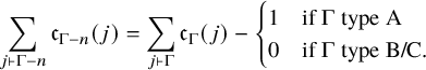 $$ \begin{align*} \sum_{j \vdash \Gamma-n} \mathfrak{c}_{\Gamma-n}(j) &= \sum_{j \vdash \Gamma} \mathfrak{c}_\Gamma(j) - \begin{cases} 1 &\text{if } \Gamma \text{ type A}\\ 0 &\text{if } \Gamma \text{ type B/C.} \end{cases} \end{align*} $$
Next, we compare the contributions to
 $D_\Gamma $
and
$D_\Gamma $
and
 $D_{\Gamma - n}$
by leaf blocks and internal blocks of size greater than
$D_{\Gamma - n}$
by leaf blocks and internal blocks of size greater than
 $2$
. By Lemmas 8.10, 8.12 and 8.13, it follows that
$2$
. By Lemmas 8.10, 8.12 and 8.13, it follows that
 $$\begin{align*}\left| LB_{\Gamma-n} \right| +\left| \{B \in \mathrm{IB}_{\Gamma-n} \mid \left| B \right|> 2\} \right| = \left| LB_\Gamma \right| + \left| \{B \in \mathrm{IB}_{\Gamma} \mid \left| B \right| > 2\} \right| - \begin{cases} 1 & \text{ if }\Gamma\text{ type A but not A2,} \\ 0 & \text{ if }\Gamma\text{ type B, C, or A2.} \end{cases} \end{align*}$$
Since
 $\Gamma $
is naturally labeled, if
$\Gamma $
is naturally labeled, if
 $s \in \mathrm {IC}_{\Gamma -n}$
(so
$s \in \mathrm {IC}_{\Gamma -n}$
(so
 $s \neq (n,n-1)$
), then the connected component of
$s \neq (n,n-1)$
), then the connected component of
 $([n-1],E(\Gamma -n) \setminus s)$
that does not contain the vertex
$([n-1],E(\Gamma -n) \setminus s)$
that does not contain the vertex
 $n-1$
is equal to the connected component of
$n-1$
is equal to the connected component of
 $([n],E(\Gamma )\setminus \{s\})$
that does not contain the vertex n. It is important for proving the recursion that for each internal cut edge
$([n],E(\Gamma )\setminus \{s\})$
that does not contain the vertex n. It is important for proving the recursion that for each internal cut edge
 $s \in \mathrm {IC}_{\Gamma - n} \subset \mathrm {IC}_\Gamma $
, we always pick the component
$s \in \mathrm {IC}_{\Gamma - n} \subset \mathrm {IC}_\Gamma $
, we always pick the component
 $G_s$
to be equal in
$G_s$
to be equal in
 $\Gamma $
and
$\Gamma $
and
 $\Gamma - n$
(i.e., always choose
$\Gamma - n$
(i.e., always choose
 $n \notin G_s \subset \Gamma $
), so we adopt this convention. If
$n \notin G_s \subset \Gamma $
), so we adopt this convention. If
 $\Gamma $
is type A2 (i.e.,
$\Gamma $
is type A2 (i.e.,
 $\mathrm {IC}_\Gamma \neq \mathrm {IC}_{\Gamma - n}$
), we remove the ‘over-counting’ from the internal cut edge
$\mathrm {IC}_\Gamma \neq \mathrm {IC}_{\Gamma - n}$
), we remove the ‘over-counting’ from the internal cut edge
 $(n-2,n-1) \in \mathrm {IC}_\Gamma $
below and get that
$(n-2,n-1) \in \mathrm {IC}_\Gamma $
below and get that
 $$\begin{align*}\sum_{s \in \mathrm{IC}_{\Gamma-n}} \genfrac(){0pt}{0}{n-1}{\left| G_s \right|} = \sum_{s \in \mathrm{IC}_{\Gamma}} \genfrac(){0pt}{0}{n-1}{\left| G_s \right|} - \begin{cases} \genfrac(){0pt}{0}{n-1}{n-2} & \Gamma \text{ is type A2}\\ 0 &\text{otherwise.} \end{cases} \end{align*}$$
Now we compute
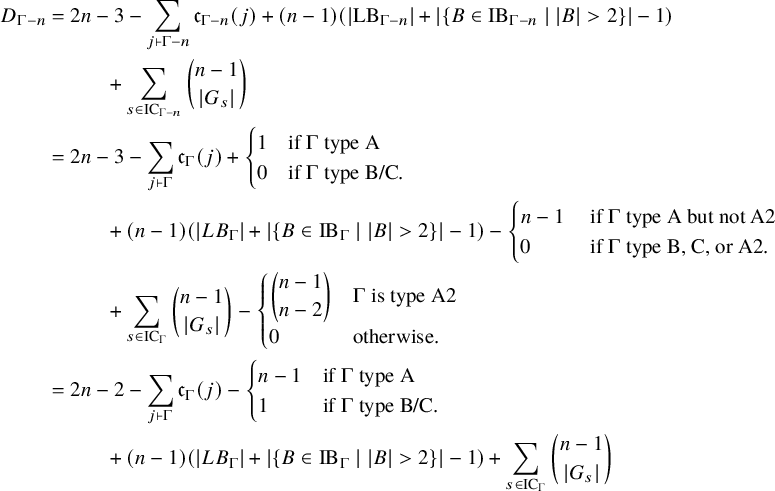 $$ \begin{align*} D_{\Gamma - n} &= 2n-3 - \sum_{j \vdash \Gamma-n} \mathfrak{c}_{\Gamma-n}(j) + (n-1)\left(\left| \mathrm{LB}_{\Gamma-n} \right| + \left| \{B \in \mathrm{IB}_{\Gamma-n} \mid \left| B \right|> 2\} \right| - 1\right) \\ &\hspace{1cm}+ \sum_{s \in \mathrm{IC}_{\Gamma-n}} \genfrac(){0pt}{0}{n-1}{\left| G_s \right|} \\ &= 2n-3 - \sum_{j \vdash \Gamma}\mathfrak{c}_{\Gamma}(j) + \begin{cases} 1 &\text{if } \Gamma \text{ type A}\\ 0 &\text{if } \Gamma \text{ type B/C.} \end{cases} \\ &\hspace{1cm} + (n-1)\left(\left| LB_\Gamma \right| + \left| \{B \in \mathrm{IB}_{\Gamma} \mid \left| B \right| > 2\} \right| - 1\right) -\begin{cases} n-1 & \text{ if }\Gamma\text{ type A but not A2} \\ 0 & \text{ if }\Gamma\text{ type B, C, or A2.} \end{cases} \\ &\hspace{1cm} + \sum_{s \in \mathrm{IC}_{\Gamma}} \genfrac(){0pt}{0}{n-1}{\left| G_s \right|} - \begin{cases} \genfrac(){0pt}{0}{n-1}{n-2} & \Gamma \text{ is type A2}\\ 0 &\text{otherwise.} \end{cases}\\ &= 2n-2 - \sum_{j \vdash \Gamma}\mathfrak{c}_{\Gamma}(j) - \begin{cases} n-1 &\text{if } \Gamma \text{ type A}\\ 1 &\text{if } \Gamma \text{ type B/C.} \end{cases} \\ &\hspace{1cm} + (n-1)\left(\left| LB_\Gamma \right| + \left| \{B \in \mathrm{IB}_{\Gamma} \mid \left| B \right| > 2\} \right| - 1\right) + \sum_{s \in \mathrm{IC}_{\Gamma}} \genfrac(){0pt}{0}{n-1}{\left| G_s \right|} \end{align*} $$
Now we have
 $D_{\Gamma -n}$
in a form that closely resembles that of
$D_{\Gamma -n}$
in a form that closely resembles that of
 $D_\Gamma $
. Recall Pascal’s identity
$D_\Gamma $
. Recall Pascal’s identity
 $\genfrac (){0pt}{0}{n}{k} = \genfrac (){0pt}{0}{n-1}{k}+\genfrac (){0pt}{0}{n-1}{k-1}$
. For each
$\genfrac (){0pt}{0}{n}{k} = \genfrac (){0pt}{0}{n-1}{k}+\genfrac (){0pt}{0}{n-1}{k-1}$
. For each
 $s \in \mathrm {IC}_\Gamma $
, we have that
$s \in \mathrm {IC}_\Gamma $
, we have that
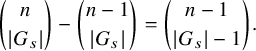 $$\begin{align*}\genfrac(){0pt}{0}{n}{\left| G_s \right|} - \genfrac(){0pt}{0}{n-1}{\left| G_s \right|} = \genfrac(){0pt}{0}{n-1}{\left| G_s \right|-1}.\end{align*}$$
In particular,
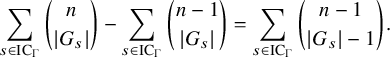 $$\begin{align*}\sum_{s \in \mathrm{IC}_\Gamma} \genfrac(){0pt}{0}{n}{\left| G_s \right|} - \sum_{s \in \mathrm{IC}_\Gamma}\genfrac(){0pt}{0}{n-1}{\left| G_s \right|} = \sum_{s \in \mathrm{IC}_\Gamma}\genfrac(){0pt}{0}{n-1}{\left| G_s \right|-1}. \end{align*}$$
So we compute that the difference
 $D_\Gamma - D_{\Gamma - n}$
is equal to
$D_\Gamma - D_{\Gamma - n}$
is equal to
 $$ \begin{align*} 1 + \left(\left| \mathrm{LB}_\Gamma \right| + \left| \{B \in \mathrm{IB}_{\Gamma} \mid \left| B \right|> 2\} \right| - 1\right) + \sum_{s \in \mathrm{IC}_\Gamma}\genfrac(){0pt}{0}{n-1}{\left| G_s \right|-1} + \begin{cases} n-1 & \text{ if }\Gamma\text{ type A} \\ 1 & \text{ if }\Gamma\text{ type B/C.} \end{cases} \end{align*} $$
The remainder of the proof is essentially the same as the proof for Lemma 8.5. In particular,
-
1. Leaf blocks of size
$2$
that do not contain the vertex n are in bijection with strongly dominant pairs
$(i,j)$
where
$\left | \Gamma _i^j \right | = 1$
, -
2. The set of internal cut edges
$\mathrm {IC}_\Gamma $
is equal to the set of strongly dominant pairs
$(i,j)$
, where
$\left | \Gamma _i^j \right |>1$
, and -
3. Leaf blocks and internal blocks of size at least three (i.e., all blocks of size at least
$3$
) that do not contain the vertex n are in bijection with weakly dominant pairs
$(i,j)$
.


We note that
 $\genfrac (){0pt}{0}{n-1}{1-1} = 1$
and get that
$\genfrac (){0pt}{0}{n-1}{1-1} = 1$
and get that
 $$\begin{align*}\left(\left| \mathrm{LB}_\Gamma \right| + \left| \{B \in \mathrm{IB}_{\Gamma} \mid \left| B \right|> 2\} \right| - 1\right) + \sum_{s \in \mathrm{IC}_\Gamma}\genfrac(){0pt}{0}{n-1}{\left| G_s \right|-1} = \sum_{(i,j) \gg \Gamma} \genfrac(){0pt}{0}{n-1}{\left| \Gamma_i^j \right|-1} + \left| \left\{(i,j) > \Gamma \right\} \right|. \end{align*}$$
Thus,
 $D_\Gamma - D_{\Gamma - n}$
has the claimed form.
$D_\Gamma - D_{\Gamma - n}$
has the claimed form.
Corollary 8.14. Let
 $\Gamma $
be a connected graph on
$\Gamma $
be a connected graph on
 $[n]$
where
$[n]$
where
 $n \geq 3$
, and
$n \geq 3$
, and
 $D_\Gamma $
as defined in Equation (8.1). Then
$D_\Gamma $
as defined in Equation (8.1). Then
 $\dim _{\mathbb {C}}(\mathcal {M}_{\Gamma }^1) = D_\Gamma $
. Moreover,
$\dim _{\mathbb {C}}(\mathcal {M}_{\Gamma }^1) = D_\Gamma $
. Moreover,
 $\dim _{\mathbb {C}}(\mathrm {L}_\Gamma )_1 = \dim _{\mathbb {C}}(\mathrm {R}_\Gamma )_1 = D_\Gamma - n$
.
$\dim _{\mathbb {C}}(\mathrm {L}_\Gamma )_1 = \dim _{\mathbb {C}}(\mathrm {R}_\Gamma )_1 = D_\Gamma - n$
.
Proof. It suffices to assume that
 $\Gamma $
is cliqued and naturally labeled. In this case, by Theorem 7.2 and Proposition 8.9, both
$\Gamma $
is cliqued and naturally labeled. In this case, by Theorem 7.2 and Proposition 8.9, both
 $\dim _{\mathbb {C}}(\mathcal {M}_{\Gamma }^1)$
and
$\dim _{\mathbb {C}}(\mathcal {M}_{\Gamma }^1)$
and
 $D_\Gamma $
follow the same recursion. Thus, it suffices to show equality on all connected graphs on
$D_\Gamma $
follow the same recursion. Thus, it suffices to show equality on all connected graphs on
 $3$
vertices. Quick computation confirms that
$3$
vertices. Quick computation confirms that
 $$\begin{align*}\dim_{\mathbb{C}}(\mathcal{M}_{K_3}^1) = 5 = D_{K_3}\text{ and } \dim_{\mathbb{C}}(\mathcal{M}_{P_3}^1) = 7 = D_{P_3},\end{align*}$$
and so the two statistics must be equal. The ‘moreover’ part follows from the fact that
 $\mathbb {C}\{\bar {t}_1,...,\bar {t}_n\}$
and
$\mathbb {C}\{\bar {t}_1,...,\bar {t}_n\}$
and
 $\mathbb {C}\{\bar {x}_1,...,\bar {x}_n\}$
are the (n-dimensional) linear subspace of
$\mathbb {C}\{\bar {x}_1,...,\bar {x}_n\}$
are the (n-dimensional) linear subspace of
 $\mathcal {M}_{\Gamma }^1$
quotiented to obtain
$\mathcal {M}_{\Gamma }^1$
quotiented to obtain
 $\mathrm {L}_\Gamma $
and
$\mathrm {L}_\Gamma $
and
 $\mathrm {R}_\Gamma $
, respectively.
$\mathrm {R}_\Gamma $
, respectively.
We now have a closed combinatorial formula for the
 $\mathbb {C}$
-dimension of the first graded piece of
$\mathbb {C}$
-dimension of the first graded piece of
 $\mathcal {M}_{\Gamma }^1$
. In particular, we have the dimension of the representations corresponding to
$\mathcal {M}_{\Gamma }^1$
. In particular, we have the dimension of the representations corresponding to
 $\mathbf {ch}\left (\mathrm {L}_{\Gamma }\right )_1$
and
$\mathbf {ch}\left (\mathrm {L}_{\Gamma }\right )_1$
and
 $\mathbf {ch}\left (\mathrm {R}_{\Gamma }\right )_1$
. We are also quite close to constructing
$\mathbf {ch}\left (\mathrm {R}_{\Gamma }\right )_1$
. We are also quite close to constructing
 $\mathbb {C}$
-bases of
$\mathbb {C}$
-bases of
 $\mathcal {M}_{\Gamma }^1$
, as the formulae for
$\mathcal {M}_{\Gamma }^1$
, as the formulae for
 $D_\Gamma $
in Lemma 8.5 and the natural one for
$D_\Gamma $
in Lemma 8.5 and the natural one for
 $\left | \mathcal {B}_\Gamma \right |$
are very similar.
$\left | \mathcal {B}_\Gamma \right |$
are very similar.
9 The left and right linear representations
This subsection computes
 $\mathbf {ch}\left (\mathrm {L}_{\Gamma }\right )_1$
and
$\mathbf {ch}\left (\mathrm {L}_{\Gamma }\right )_1$
and
 $\mathbf {ch}\left (\mathrm {R}_{\Gamma }\right )_1$
for all connected
$\mathbf {ch}\left (\mathrm {R}_{\Gamma }\right )_1$
for all connected
 $\Gamma $
, proving Theorem 1.4 from the introduction. We prove this assuming that
$\Gamma $
, proving Theorem 1.4 from the introduction. We prove this assuming that
 $\Gamma $
is naturally labeled and get the label-independent formula as a corollary. The computation is direct and achieved by computing the dot action on two subsets
$\Gamma $
is naturally labeled and get the label-independent formula as a corollary. The computation is direct and achieved by computing the dot action on two subsets
 $\mathcal {LS}_\Gamma $
and
$\mathcal {LS}_\Gamma $
and
 $\mathcal {RS}_\Gamma $
of
$\mathcal {RS}_\Gamma $
of
 $\mathcal {B}_\Gamma $
that project to bases of
$\mathcal {B}_\Gamma $
that project to bases of
 $(\mathrm {L}_{\Gamma })_1$
and
$(\mathrm {L}_{\Gamma })_1$
and
 $(\mathrm {R}_{\Gamma })_1$
, respectively.
$(\mathrm {R}_{\Gamma })_1$
, respectively.
Say
 $\Gamma $
is a naturally labeled connected graph. By Proposition 6.12 and Theorem 7.2, if
$\Gamma $
is a naturally labeled connected graph. By Proposition 6.12 and Theorem 7.2, if

then
 $\mathcal {M}_{\Gamma }^1 = \mathbb {C}\mathcal {B}_{\Gamma }$
. For the first graded piece of
$\mathcal {M}_{\Gamma }^1 = \mathbb {C}\mathcal {B}_{\Gamma }$
. For the first graded piece of
 $\mathrm {L}_{\Gamma }$
and
$\mathrm {L}_{\Gamma }$
and
 $\mathrm {R}_{\Gamma }$
, we will remove elements from
$\mathrm {R}_{\Gamma }$
, we will remove elements from
 $\mathcal {B}_\Gamma $
using the relations in Lemma 5.5, prove that the image of what remains is a basis by dimension, and then compute the representations on
$\mathcal {B}_\Gamma $
using the relations in Lemma 5.5, prove that the image of what remains is a basis by dimension, and then compute the representations on
 $(\mathrm {L}_{\Gamma })_1$
and
$(\mathrm {L}_{\Gamma })_1$
and
 $(\mathrm {R}_{\Gamma })_1$
using Lemma 9.1 below.
$(\mathrm {R}_{\Gamma })_1$
using Lemma 9.1 below.
Lemma 9.1. Let
 $w \in S_n$
. Then
$w \in S_n$
. Then
 $$\begin{align*}w \cdot \bar{f}_A^{(i,j)} = \bar{f}_{w(A)}^{(i,j)} \text{ and } w \cdot \bar{y}_{r,k}^j = \bar{y}_{r,w(k)}^j.\end{align*}$$
The proof of Lemma 9.1 is direct from the definitions.
Now we will define two subsets of
 $\mathcal {B}_\Gamma $
– one for
$\mathcal {B}_\Gamma $
– one for
 $(\mathrm {L}_{\Gamma })_1$
and one for
$(\mathrm {L}_{\Gamma })_1$
and one for
 $(\mathrm {R}_{\Gamma })_1$
– that project to
$(\mathrm {R}_{\Gamma })_1$
– that project to
 $\mathbb {C}$
-bases in these quotients.
$\mathbb {C}$
-bases in these quotients.
For the linear piece of the left quotient
 $(\mathrm {L}_{\Gamma })_1$
, we first remove from
$(\mathrm {L}_{\Gamma })_1$
, we first remove from
 $\mathcal {B}_\Gamma $
the splines
$\mathcal {B}_\Gamma $
the splines
 $\{\bar {t}_1,...,\bar {t}_n\}$
. We may also discard
$\{\bar {t}_1,...,\bar {t}_n\}$
. We may also discard
-
(1) The single spline
$\bar {x}_n$
by Lemma 5.5(1), -
(2) The splines
$\{\bar {x}_i \mid (i,j) \gg \Gamma \}$
by Lemma 5.5(2), and -
(3) The splines
$\{\bar {x}_i \mid (i,j)> \Gamma \}$
by Lemma 5.5(3).


Note the set of splines in (2) and (3) is size
 $\left | \{\bar {x}_i \mid (i,j) \gg \Gamma \} \cup \{\bar {x}_i \mid (i,j)> \Gamma \} \right | = \sum\limits _{j \vdash \Gamma } \mathfrak {c}(j)$
. So the image of
$\left | \{\bar {x}_i \mid (i,j) \gg \Gamma \} \cup \{\bar {x}_i \mid (i,j)> \Gamma \} \right | = \sum\limits _{j \vdash \Gamma } \mathfrak {c}(j)$
. So the image of
in
 $(\mathrm {L}_{\Gamma })_1$
is a spanning set. Note that the size of
$(\mathrm {L}_{\Gamma })_1$
is a spanning set. Note that the size of
 $\left \{\bar {x}_r \in \mathcal {X}_{n-1} \mid r\right .$
is not s-dominant
$\left \{\bar {x}_r \in \mathcal {X}_{n-1} \mid r\right .$
is not s-dominant
 $\left .\forall s\in [n]\right \}$
is
$\left .\forall s\in [n]\right \}$
is
 $n-1-\sum\limits _{j\vdash \Gamma } \mathfrak {c}(j)$
, the size of
$n-1-\sum\limits _{j\vdash \Gamma } \mathfrak {c}(j)$
, the size of
 $\left \{\bar {f}_A^s \mid s \gg \Gamma \right \}$
is
$\left \{\bar {f}_A^s \mid s \gg \Gamma \right \}$
is
 ${ \sum\limits _{(i,j) \gg \Gamma } \genfrac (){0pt}{0}{n}{\left | \Gamma _i^j \right |}}$
, and the size of
${ \sum\limits _{(i,j) \gg \Gamma } \genfrac (){0pt}{0}{n}{\left | \Gamma _i^j \right |}}$
, and the size of
 $\left \{\bar {y}_{r,k}^j \left | (r,j)> \Gamma ,\;\; k \in [n]\right .\right \}$
is
$\left \{\bar {y}_{r,k}^j \left | (r,j)> \Gamma ,\;\; k \in [n]\right .\right \}$
is
 ${ \sum\limits_{(i,j)> \Gamma }n}$
. Thus, the size of
${ \sum\limits_{(i,j)> \Gamma }n}$
. Thus, the size of
 $\mathcal {LS}_\Gamma $
is precisely the dimension
$\mathcal {LS}_\Gamma $
is precisely the dimension
 $D_\Gamma - n$
of
$D_\Gamma - n$
of
 $(\mathrm {L}_{\Gamma })_1$
, as computed in Lemma 8.5. So
$(\mathrm {L}_{\Gamma })_1$
, as computed in Lemma 8.5. So
 $\mathcal {LS}_\Gamma $
projects to a basis of
$\mathcal {LS}_\Gamma $
projects to a basis of
 $(\mathrm {L}_{\Gamma })_1$
. In fact,
$(\mathrm {L}_{\Gamma })_1$
. In fact,
 $\mathcal {LS}_\Gamma $
is a permutation basis for the dot action representation, from which it is easy to compute the dot action representation (we will state and prove this in Theorem 9.2).
$\mathcal {LS}_\Gamma $
is a permutation basis for the dot action representation, from which it is easy to compute the dot action representation (we will state and prove this in Theorem 9.2).
For the linear piece of the right quotient
 $(\mathrm {R}_{\Gamma })_1$
, we first remove from
$(\mathrm {R}_{\Gamma })_1$
, we first remove from
 $\mathcal {B}_\Gamma $
the splines
$\mathcal {B}_\Gamma $
the splines
 $\{\bar {x}_1,...,\bar {x}_n\}$
. Let
$\{\bar {x}_1,...,\bar {x}_n\}$
. Let ![]() , and let
, and let
 $\left \{A_p \mid p \in \left [\genfrac (){0pt}{0}{n}{m_{ij}}\right ]\right \}$
be an enumeration of the
$\left \{A_p \mid p \in \left [\genfrac (){0pt}{0}{n}{m_{ij}}\right ]\right \}$
be an enumeration of the
 $\genfrac (){0pt}{0}{n}{m_{ij}}$
-many subsets A associated to a strongly dominant pair
$\genfrac (){0pt}{0}{n}{m_{ij}}$
-many subsets A associated to a strongly dominant pair
 $(i,j) \gg \Gamma $
. By Lemma 5.5, the following three relations hold in
$(i,j) \gg \Gamma $
. By Lemma 5.5, the following three relations hold in
 $\mathrm {R}_{\Gamma }$
:
$\mathrm {R}_{\Gamma }$
:
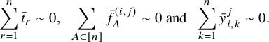 $$\begin{align*}\sum_{r=1}^n \bar{t}_r \sim 0,\;\; \sum_{A \subset [n]} \bar{f}_A^{(i,j)} \sim 0 \; \text{and}\;\; \sum_{k=1}^n \bar{y}_{i,k}^j \sim 0.\end{align*}$$
The natural subset of
 $\mathcal {B}_\Gamma $
whose image spans
$\mathcal {B}_\Gamma $
whose image spans
 $(\mathrm {R}_{\Gamma })_1$
is therefore
$(\mathrm {R}_{\Gamma })_1$
is therefore

The first subset is size
 $n-1$
. The second subset is size
$n-1$
. The second subset is size
 ${ \sum\limits _{(i,j)\gg \Gamma } \left (\genfrac (){0pt}{0}{n}{\left | \Gamma _i^j \right |} - 1 \right )}$
, and the third subset is size
${ \sum\limits _{(i,j)\gg \Gamma } \left (\genfrac (){0pt}{0}{n}{\left | \Gamma _i^j \right |} - 1 \right )}$
, and the third subset is size
 ${ \sum\limits _{(i,j)>\Gamma } (n-1) }$
. The number of (strong or weak) dominant pairs is
${ \sum\limits _{(i,j)>\Gamma } (n-1) }$
. The number of (strong or weak) dominant pairs is
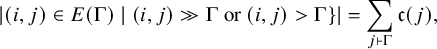 $$\begin{align*}\left| (i,j) \in E(\Gamma) \mid (i,j) \gg \Gamma \text{ or } (i,j)> \Gamma\} \right| = \sum_{j \vdash \Gamma} \mathfrak{c}(j),\end{align*}$$
so
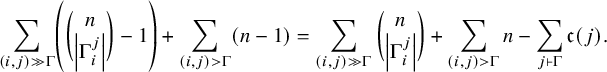 $$\begin{align*}\sum_{(i,j)\gg \Gamma} \left(\genfrac(){0pt}{0}{n}{\left| \Gamma_i^j \right|} - 1 \right)+ \sum_{(i,j)>\Gamma} (n-1) = \sum_{(i,j)\gg \Gamma} \genfrac(){0pt}{0}{n}{\left| \Gamma_i^j \right|} + \sum_{(i,j)>\Gamma} n -\sum_{j \vdash \Gamma}\mathfrak{c}(j). \end{align*}$$
So the image of
 $\mathcal {RS}_\Gamma $
is a basis for
$\mathcal {RS}_\Gamma $
is a basis for
 $(\mathrm {R}_{\Gamma })_1$
.
$(\mathrm {R}_{\Gamma })_1$
.
Theorem 9.2. Let
 $\Gamma $
be a naturally labeled graph. If
$\Gamma $
be a naturally labeled graph. If
 $(i,j) \gg \Gamma $
, define the partition
$(i,j) \gg \Gamma $
, define the partition ![]() (reordered if necessary). Then
(reordered if necessary). Then
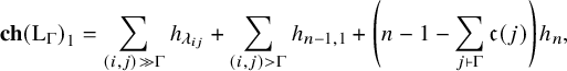 $$\begin{align*}\mathbf{ch}\left(\mathrm{L}_{\Gamma}\right)_1 = \sum_{(i,j) \gg \Gamma} h_{\lambda_{ij}} + \sum_{(i,j)> \Gamma} h_{n-1,1} + \left(n-1-\sum_{j \vdash \Gamma} \mathfrak{c}(j)\right) h_n, \end{align*}$$
and
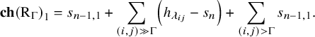 $$\begin{align*}\mathbf{ch}\left(\mathrm{R}_{\Gamma}\right)_1 = s_{n-1,1} + \sum_{(i,j) \gg \Gamma} \left(h_{\lambda_{ij}}-s_n\right) + \sum_{(i,j)> \Gamma} s_{n-1,1}. \end{align*}$$
Proof. Since
 $\mathbb {C}\mathcal {LS}_\Gamma $
and
$\mathbb {C}\mathcal {LS}_\Gamma $
and
 $\mathbb {C}\mathcal {RS}_\Gamma $
are
$\mathbb {C}\mathcal {RS}_\Gamma $
are
 $S_n$
-invariant vector spaces, the dot action on each is a representation. Since the projection of these spaces to
$S_n$
-invariant vector spaces, the dot action on each is a representation. Since the projection of these spaces to
 $(\mathrm {L}_{\Gamma })_1$
and
$(\mathrm {L}_{\Gamma })_1$
and
 $(\mathrm {R}_{\Gamma })_1$
are in fact isomorphisms, the symmetric functions
$(\mathrm {R}_{\Gamma })_1$
are in fact isomorphisms, the symmetric functions
 $\mathbf {ch}\left (\mathrm {L}_{\Gamma }\right )_1$
and
$\mathbf {ch}\left (\mathrm {L}_{\Gamma }\right )_1$
and
 $\mathbf {ch}\left (\mathrm {R}_{\Gamma }\right )_1$
are the characters of the dot action representation on
$\mathbf {ch}\left (\mathrm {R}_{\Gamma }\right )_1$
are the characters of the dot action representation on
 $\mathbb {C}\mathcal {LS}_\Gamma $
and
$\mathbb {C}\mathcal {LS}_\Gamma $
and
 $\mathbb {C}\mathcal {RS}_\Gamma $
, respectively. Each of the identified subsets in bases
$\mathbb {C}\mathcal {RS}_\Gamma $
, respectively. Each of the identified subsets in bases
 $\mathcal {LS}_\Gamma $
and
$\mathcal {LS}_\Gamma $
and
 $\mathcal {RS}_\Gamma $
span
$\mathcal {RS}_\Gamma $
span
 $S_n$
-invariant subspaces of
$S_n$
-invariant subspaces of
 $\mathbb {C}\mathcal {LS}_\Gamma $
and
$\mathbb {C}\mathcal {LS}_\Gamma $
and
 $\mathbb {C}\mathcal {RS}_\Gamma $
, respectively.
$\mathbb {C}\mathcal {RS}_\Gamma $
, respectively.
First, we will compute each part of
 $\mathbf {ch}\left (\mathrm {L}_{\Gamma }\right )_1$
. The dot action fixes each
$\mathbf {ch}\left (\mathrm {L}_{\Gamma }\right )_1$
. The dot action fixes each
 $\bar {x}_i$
, and so the character of the dot action representation on
$\bar {x}_i$
, and so the character of the dot action representation on
 $\mathbb {C}\left \{\bar {x}_r \in \mathcal {X}_{n-1} \mid r\right .$
is not s-dominant
$\mathbb {C}\left \{\bar {x}_r \in \mathcal {X}_{n-1} \mid r\right .$
is not s-dominant
 $\left .\forall s\in [n]\right \}$
is
$\left .\forall s\in [n]\right \}$
is
 ${ \left (n-1-\sum\limits _{j \vdash \Gamma } \mathfrak {c}(j)\right ) h_n}$
. By Lemma 9.1, the character of the dot action representation restricted to
${ \left (n-1-\sum\limits _{j \vdash \Gamma } \mathfrak {c}(j)\right ) h_n}$
. By Lemma 9.1, the character of the dot action representation restricted to
 $\mathbb {C}\left \{\bar {f}_A^s \mid s \gg \Gamma \right \}$
is
$\mathbb {C}\left \{\bar {f}_A^s \mid s \gg \Gamma \right \}$
is
 ${ \sum\limits _{(i,j) \gg \Gamma } h_{\lambda _{ij}}}$
. By Lemma 9.1 as well, the character of the dot action representation on
${ \sum\limits _{(i,j) \gg \Gamma } h_{\lambda _{ij}}}$
. By Lemma 9.1 as well, the character of the dot action representation on
 $\mathbb {C}\left \{\bar {y}_{r,k}^j \left | (r,j)> \Gamma ,\;\; k \in [n]\right .\right \}$
is
$\mathbb {C}\left \{\bar {y}_{r,k}^j \left | (r,j)> \Gamma ,\;\; k \in [n]\right .\right \}$
is
 ${ \sum\limits _{(i,j)> \Gamma } h_{n-1,1}}$
.
${ \sum\limits _{(i,j)> \Gamma } h_{n-1,1}}$
.
Now we will compute each part of
 $\mathbf {ch}\left (\mathrm {R}_{\Gamma }\right )_1$
. Each of the following computations use the same principle argument. If K is an integer, and the set
$\mathbf {ch}\left (\mathrm {R}_{\Gamma }\right )_1$
. Each of the following computations use the same principle argument. If K is an integer, and the set
 $\{e_i \mid i \in [K]\}$
is a permutation basis of some permutation representation of
$\{e_i \mid i \in [K]\}$
is a permutation basis of some permutation representation of
 $S_n$
with character
$S_n$
with character
 $h_\lambda $
, then the vector
$h_\lambda $
, then the vector
 ${ \sum\limits _{i=1}^K e_i}$
is invariant under that representation. Furthermore, the character of the representation on the orthogonal subspace spanned by
${ \sum\limits _{i=1}^K e_i}$
is invariant under that representation. Furthermore, the character of the representation on the orthogonal subspace spanned by
 $\{e_{i+1} - e_{i} \mid i \in [K-1]\}$
is
$\{e_{i+1} - e_{i} \mid i \in [K-1]\}$
is
 $h_\lambda - s_n$
.
$h_\lambda - s_n$
.
The character of the dot action representation on
 $\mathbb {C}\{t_i \mid i \in [n]\}$
is
$\mathbb {C}\{t_i \mid i \in [n]\}$
is
 $h_{n-1,n}$
, and so the dot action representation on
$h_{n-1,n}$
, and so the dot action representation on
 $\mathbb {C}\{\bar {t}_r-\bar {t}_{r+1} \mid r \in [n-1]\}$
is
$\mathbb {C}\{\bar {t}_r-\bar {t}_{r+1} \mid r \in [n-1]\}$
is
 $h_{n-1,n}-s_n = s_{n-1,1}$
. The character of the dot action representation on
$h_{n-1,n}-s_n = s_{n-1,1}$
. The character of the dot action representation on
 $\mathbb {C}\left \{ \bar {f}_{A_p}^{(i,j)}\left | p \in \left [\genfrac (){0pt}{0}{n}{m_i}\right ], \; (i,j) \gg \Gamma \right .\right \}$
is
$\mathbb {C}\left \{ \bar {f}_{A_p}^{(i,j)}\left | p \in \left [\genfrac (){0pt}{0}{n}{m_i}\right ], \; (i,j) \gg \Gamma \right .\right \}$
is
 ${ \sum\limits _{(i,j) \gg \Gamma } h_{\lambda _{ij}}}$
, and so the character of the dot action representation on
${ \sum\limits _{(i,j) \gg \Gamma } h_{\lambda _{ij}}}$
, and so the character of the dot action representation on
 $\mathbb {C}\left \{ \bar {f}_{A_p}^{(i,j)} - \bar {f}_{A_{p+1}}^{(i,j)} \left | p \in \left [\genfrac (){0pt}{0}{n}{m_i}-1\right ], \; (i,j) \gg \Gamma \right .\right \}$
is
$\mathbb {C}\left \{ \bar {f}_{A_p}^{(i,j)} - \bar {f}_{A_{p+1}}^{(i,j)} \left | p \in \left [\genfrac (){0pt}{0}{n}{m_i}-1\right ], \; (i,j) \gg \Gamma \right .\right \}$
is
 ${ \sum\limits _{(i,j) \gg \Gamma } h_{\lambda _{ij}} - s_n}$
. The character of the dot action representation on
${ \sum\limits _{(i,j) \gg \Gamma } h_{\lambda _{ij}} - s_n}$
. The character of the dot action representation on
 $\mathbb {C}\left \{ \left .\bar {y}_{r,k}^{j}\right | (r,j)> \Gamma ,\; k\in [n] \right \}$
is
$\mathbb {C}\left \{ \left .\bar {y}_{r,k}^{j}\right | (r,j)> \Gamma ,\; k\in [n] \right \}$
is
 ${ \sum \limits_{(i,j)> \Gamma } h_{n-1,1}}$
, and so the character of the dot action representation on
${ \sum \limits_{(i,j)> \Gamma } h_{n-1,1}}$
, and so the character of the dot action representation on
 $\mathbb {C} \left \{\left. \bar {y}_{r,k}^{j} - \bar {y}_{r,k+1}^j \right | (r,j)> \Gamma ,\; k\in [n-1] \right \}$
is
$\mathbb {C} \left \{\left. \bar {y}_{r,k}^{j} - \bar {y}_{r,k+1}^j \right | (r,j)> \Gamma ,\; k\in [n-1] \right \}$
is
 ${ \sum\limits _{(i,j)> \Gamma }(h_{n-1,1}-s_n) = \sum\limits _{(i,j) > \Gamma }s_{n-1,1}}$
.
${ \sum\limits _{(i,j)> \Gamma }(h_{n-1,1}-s_n) = \sum\limits _{(i,j) > \Gamma }s_{n-1,1}}$
.
The Schur-expansion of
 $h_{\lambda _{ij}}$
is easy to compute since
$h_{\lambda _{ij}}$
is easy to compute since
 $\lambda _{ij}$
is only a two-part partition. In particular, if K is the larger of
$\lambda _{ij}$
is only a two-part partition. In particular, if K is the larger of
 $\left | \Gamma _i^j \right |$
and
$\left | \Gamma _i^j \right |$
and
 $n-\left | \Gamma _i^j \right |$
, then
$n-\left | \Gamma _i^j \right |$
, then
 ${ h_{\lambda _{ij}}-s_n = \sum\limits _{m=0}^{n-K-1} s_{K+m,n-K-m}}$
.
${ h_{\lambda _{ij}}-s_n = \sum\limits _{m=0}^{n-K-1} s_{K+m,n-K-m}}$
.
The following corollary gives the label-independent description, from the statistics on block-cut trees described in Section 8.
Corollary 9.3. Let
 $\Gamma $
be a connected simple graph, and let
$\Gamma $
be a connected simple graph, and let
 $\mathrm {LB}_\Gamma $
,
$\mathrm {LB}_\Gamma $
,
 $\mathrm {IB}_\Gamma $
and
$\mathrm {IB}_\Gamma $
and
 $\mathrm {IC}_\Gamma $
be the leaf blocks, internal blocks and internal cut edges of
$\mathrm {IC}_\Gamma $
be the leaf blocks, internal blocks and internal cut edges of
 $\Gamma $
as defined in the beginning of Section 8. For
$\Gamma $
as defined in the beginning of Section 8. For
 $(i,j) \in \mathrm {IC}_\Gamma $
, let
$(i,j) \in \mathrm {IC}_\Gamma $
, let
 $\lambda _{ij}$
be the partition
$\lambda _{ij}$
be the partition
 $\left (n-\left | G_{(i,j)} \right |,\left | G_{(i,j)} \right |\right )$
(reordered if necessary), where
$\left (n-\left | G_{(i,j)} \right |,\left | G_{(i,j)} \right |\right )$
(reordered if necessary), where
 $G_{(i,j)}$
is a connected component of the graph
$G_{(i,j)}$
is a connected component of the graph
 $\left ([n],E(\Gamma )\setminus \{(i,j)\}\right )$
. Then
$\left ([n],E(\Gamma )\setminus \{(i,j)\}\right )$
. Then
 $$\begin{align*}\mathbf{ch}\left(\mathrm{L}_{\Gamma}\right)_1 = \sum_{(i,j) \in \mathrm{IC}_\Gamma} h_{\lambda_{ij}} + \left( \left| \mathrm{LB}_\Gamma \right| + \left| \{B \in \mathrm{IB}_\Gamma \mid \left| B \right|> 2\} \right| - 1\right) h_{n-1,1} + \left(n-1-\sum_{j \vdash \Gamma} \mathfrak{c}(j)\right) h_n, \end{align*}$$
and
 $$\begin{align*}\mathbf{ch}\left(\mathrm{R}_{\Gamma}\right)_1 =\sum_{(i,j) \in \mathrm{IC}_\Gamma} \left(h_{\lambda_{ij}}-s_n\right) + \left( \left| \mathrm{LB}_\Gamma \right| + \left| \{B \in \mathrm{IB}_\Gamma \mid \left| B \right|> 2\} \right|\right)s_{n-1,1}. \end{align*}$$
Proof. This follows directly from Theorem 9.2 and the bijections/equalities described in the proof of Lemma 8.5 (and also the proof of Proposition 8.9).
We note that in the statement of Theorem 1.4 in the introduction, the sets are
 $E_1 = \mathrm {IC}_\Gamma $
and
$E_1 = \mathrm {IC}_\Gamma $
and
 $E_2 = \mathrm {LB}_\Gamma \cup \{B \in \mathrm {IB}_\Gamma \mid \left | B \right |> 2\}$
, and the integer
$E_2 = \mathrm {LB}_\Gamma \cup \{B \in \mathrm {IB}_\Gamma \mid \left | B \right |> 2\}$
, and the integer
 $k = n-1-\sum\limits _{j \vdash \Gamma } \mathfrak {c}(j)$
.
$k = n-1-\sum\limits _{j \vdash \Gamma } \mathfrak {c}(j)$
.
Example 9.4. Let
 $\Gamma $
be the graph from Example 8.6. We may compute the representations with either Theorem 9.2 or Corollary 9.3. Then
$\Gamma $
be the graph from Example 8.6. We may compute the representations with either Theorem 9.2 or Corollary 9.3. Then
 $$\begin{align*}\mathbf{ch}\left(\mathrm{L}_{\Gamma}\right)_1 = 6h_{12} + 4h_{11,1} + h_{8,4}\end{align*}$$
and
 $$\begin{align*}\mathbf{ch}\left(\mathrm{R}_{\Gamma}\right)_1 = 4s_{11,1} + h_{8,4}-s_{12} = 4s_{11,1} + (s_{8,4} + s_{9,3} + s_{10,2} + s_{11,1}).\end{align*}$$
We note that, by this formula, the symmetric function
 $\mathbf {ch}\left (\mathrm {L}_{\Gamma }\right )_1$
is h-positive for all graphs
$\mathbf {ch}\left (\mathrm {L}_{\Gamma }\right )_1$
is h-positive for all graphs
 $\Gamma $
. So Theorem 9.2 and Corollary 9.3 prove an extension of the linear part of the graded Stanley–Stembridge conjecture from Hessenberg graphs to all connected graphs.
$\Gamma $
. So Theorem 9.2 and Corollary 9.3 prove an extension of the linear part of the graded Stanley–Stembridge conjecture from Hessenberg graphs to all connected graphs.
A Tables of polynomials
Without geometric methods, it is quite difficult to compute these representations. One can, however, compute the dimension more easily using [Reference Grayson and Stillman17, 24]. For example, despite our current inability to compute the representation, we do know that
 $\dim (\mathrm {L}_{C_4})_3 = 9 = \dim (\mathrm {R}_{C_4})_3$
. We also note that
$\dim (\mathrm {L}_{C_4})_3 = 9 = \dim (\mathrm {R}_{C_4})_3$
. We also note that
 $\mathcal {M}_{C_4}^{\leq 3}$
is not a free module, but
$\mathcal {M}_{C_4}^{\leq 3}$
is not a free module, but
 $\mathcal {M}_{C_4}^{\leq 2}$
is free (and
$\mathcal {M}_{C_4}^{\leq 2}$
is free (and
 $\mathbf {ch}\left (\mathrm {L}_{C_4}\right )$
is, in degree
$\mathbf {ch}\left (\mathrm {L}_{C_4}\right )$
is, in degree
 $\leq 2$
, h-positive).
$\leq 2$
, h-positive).
Table 1 The polynomials
 $\sum\limits_{i\geq 0 }\mathbf {ch}{\left ({\mathrm {L}}_{\Gamma }\right )}_i {q}^{i}$
in the homogeneous basis and
$\sum\limits_{i\geq 0 }\mathbf {ch}{\left ({\mathrm {L}}_{\Gamma }\right )}_i {q}^{i}$
in the homogeneous basis and
 $\sum\limits_{i\geq 0 }\mathbf {ch}{\left ({\mathrm {R}}_{\Gamma }\right )}_i{q}^{i}$
in the Schur basis for all graphs on 3 and 4 vertices, excluding
$\sum\limits_{i\geq 0 }\mathbf {ch}{\left ({\mathrm {R}}_{\Gamma }\right )}_i{q}^{i}$
in the Schur basis for all graphs on 3 and 4 vertices, excluding
 $\mathbf {ch}{\left ({\mathrm {L}}_{C_4}\right )}_{3}$
and
$\mathbf {ch}{\left ({\mathrm {L}}_{C_4}\right )}_{3}$
and
 $\mathbf {ch}{\left ({\mathrm {R}}_{C_4}\right )}_{3}$
.
$\mathbf {ch}{\left ({\mathrm {R}}_{C_4}\right )}_{3}$
.
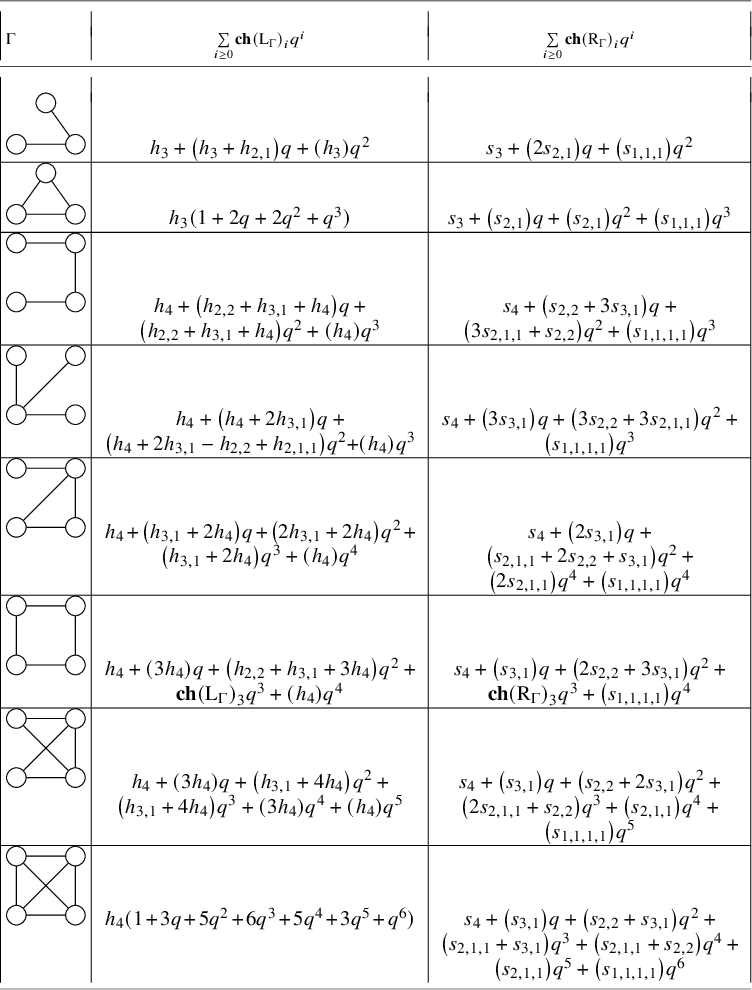
Table 2 The rank-generating functions and total rank for all isomorphism classes of graphs on 5 vertices. Geometric cases are marked with
 $\dagger $
.
$\dagger $
.
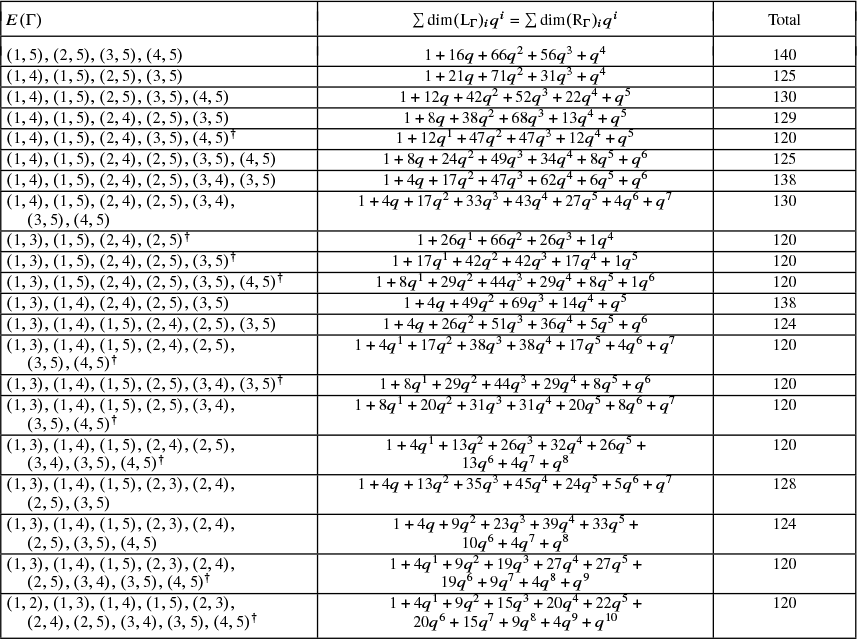
Acknowledgements
The author is grateful to Martha Precup and John Shareshian for their continued advise and support, and is thankful for several helpful conversations with Devin Akman, Laura Escobar-Vega, Matt Kerr, Jodi McWhirter, Edward Richmond and Jay Yang. We appreciate as well the helpful revisions and comments from the reviewers and editors. A majority of this work was completed while the author was a PhD Student at Washington University in St. Louis.
Competing interest
The authors have no competing interests to declare.
Financial support
This research was partially supported by NSF grant DMS-1954001.


 Open access