


1 Introduction
Convex polytopes, or more generally convex bodies, are classical and important objects in geometry. There are many results in which structures or properties of convex polytopes are shown to have deep connections with other objects, through algebraic or combinatorial procedures. Among other such results, there is the Delzant construction [Reference Delzant4], which is well known in symplectic geometry. Using the Delzant construction one obtains a natural bijective correspondence between the set of Delzant polytopes and the set of symplectic toric manifolds. Under this correspondence, the geometric data of symplectic toric manifolds are encoded as combinatorial or topological properties of their corresponding polytopes. For example, the cohomology ring of symplectic toric manifolds can be recovered completely as the Stanley–Reisner ring of the associated polytope. See (e.g., [Reference Buchstaber and Panov3]) for more details on this dictionary between Delzant polytopes and symplectic toric manifolds.
The purpose of our project is to further develop aspects of this kind of correspondence from the viewpoint of Riemannian or metric geometry. The present paper contains two parts. Firstly, we establish relationships between three natural distance functions on the set of convex bodies. The first function $d^W$
is defined by the Wasserstein distance of probability measures associated with convex bodies. The Wasserstein distance is a quite important tool in recent developments of geometric analysis for metric measure spaces. The second distance
$d^W$
is defined by the Wasserstein distance of probability measures associated with convex bodies. The Wasserstein distance is a quite important tool in recent developments of geometric analysis for metric measure spaces. The second distance $d^V$
is defined by the Lebesgue volume of the symmetric difference of convex bodies. This distance function is natural from the viewpoint of symplectic geometry and is studied in [Reference Pelayo, Pires, Ratiu and Sabatini14] and [Reference Fujita and Ohashi6]. The third function
$d^V$
is defined by the Lebesgue volume of the symmetric difference of convex bodies. This distance function is natural from the viewpoint of symplectic geometry and is studied in [Reference Pelayo, Pires, Ratiu and Sabatini14] and [Reference Fujita and Ohashi6]. The third function $d^H$
is the Hausdorff distance, which is a classical and basic tool in geometry of convex bodies. The main result of the first part of this paper is as follows.
$d^H$
is the Hausdorff distance, which is a classical and basic tool in geometry of convex bodies. The main result of the first part of this paper is as follows.
Theorem 1 (Theorem 3.1.3).
The metric topologies on the space of convex bodies determined by the distance functions $d^W$
,
$d^W$
, $d^V$
, and
$d^V$
, and $d^H$
coincide with each other.
$d^H$
coincide with each other.
Secondly, we investigate the relationship between the metric geometry of Delzant polytopes and the Riemannian geometry of symplectic toric manifolds through the Delzant construction. Here we equip each symplectic toric manifold with a Kähler metric which we call the Guillemin metric [Reference Guillemin9], and we regard a symplectic toric manifold as a Riemannian manifold. The main results in the second part of this paper are the following.
Theorem 2 (Theorem 5.2.2).
For a sequence of Delzant polytopes $\{P_i\}_i$
in
$\{P_i\}_i$
in $\mathbb {R}^n$
, suppose that
$\mathbb {R}^n$
, suppose that $\{P_i\}_i$
converges to a Delzant polytope P in
$\{P_i\}_i$
converges to a Delzant polytope P in $\mathbb {R}^n$
in the
$\mathbb {R}^n$
in the $d^H$
-topology (hence also in the
$d^H$
-topology (hence also in the $d^W$
-topology and
$d^W$
-topology and $d^V$
-topology), and the limit of the numbers of facets of
$d^V$
-topology), and the limit of the numbers of facets of $\{P_i\}_i$
coincides with that of P. Then the sequence of symplectic toric manifolds
$\{P_i\}_i$
coincides with that of P. Then the sequence of symplectic toric manifolds $\{M_{P_i}\}_i$
converges to
$\{M_{P_i}\}_i$
converges to $M_P$
with respect to the corresponding Guillemin metrics in the torus-equivariant Gromov–Hausdorff topology.
$M_P$
with respect to the corresponding Guillemin metrics in the torus-equivariant Gromov–Hausdorff topology.
As a corollary (Corollary 5.2.3), we also have a torus-equivariant stability theorem in the setting of converging symplectic toric manifolds.
The above result suggests a continuity of the one direction of the Delzant construction, from P to $M_P$
. We also have results concerning the converse direction. The following are their rough statements.
$M_P$
. We also have results concerning the converse direction. The following are their rough statements.
Theorem 3 (Theorem 5.3.1, Theorem 5.3.2).
For a sequence of Delzant polytopes $\{P_i\}_i$
in
$\{P_i\}_i$
in $\mathbb {R}^n$
and a Delzant polytope P in
$\mathbb {R}^n$
and a Delzant polytope P in $\mathbb {R}^n$
, suppose that the corresponding sequence of symplectic toric manifolds
$\mathbb {R}^n$
, suppose that the corresponding sequence of symplectic toric manifolds $\{M_{P_i}\}_i$
converges to
$\{M_{P_i}\}_i$
converges to $M_P$
with respect to the corresponding Guillemin metrics in the torus-equivariant measured Gromov–Hausdorff topology. Then we have:
$M_P$
with respect to the corresponding Guillemin metrics in the torus-equivariant measured Gromov–Hausdorff topology. Then we have:
-
• if $\{P_i\}_i$
is contained in a large ball, the fixed point set of
$M_{P_i}$
converges to that of
$M_P$
. In particular we have the lower semi-continuity of the Euler characteristic, and
$\{P_i\}_i$
is contained in a large ball, the fixed point set of
$M_{P_i}$
converges to that of
$M_P$
. In particular we have the lower semi-continuity of the Euler characteristic, and -
• we have a sequence of maps
$\{\hat f_i : P_i\to P\}_i$
such that
$\{\overline {\hat f_i(P_i)}\}_i$
converges to P in
$d^H$
-topology by using the approximation maps for
$\{M_{P_i}\}_i$
. See Theorem 5.3.2 for the precise statement.


We emphasize that there are no hypotheses on the curvature in the statement of the above theorem. By incorporating “potential functions”as in [Reference Abreu1] we may treat more general torus-invariant Riemannian metrics of symplectic toric manifolds which are not necessarily Guillemin metrics.
In the present paper, we only consider the non-collapsing case. It is surely interesting to attack the same problems under collapsing limit, and we will discuss this in a subsequent paper. In addition, our general setting of convex bodies in the first part of this paper is motivated by the fact that non-Delzant polytopes are increasingly important in the context of toric degenerations of integrable systems or projective varieties as in [Reference Harada and Kaveh10], [Reference Nishinou, Nohara and Ueda13] and so on.
This paper is organized as follows. In Section 2, we introduce three distance functions on the set of convex bodies. In Section 3, we show that the three corresponding metric topologies coincide. Note that the equivalence between the distance function defined by the volume and the Hausdorff distance is classically known, by [Reference Shephard and Webster15] for example. In [Reference Pelayo, Pires, Ratiu and Sabatini14] Pelayo–Pires–Ratiu–Sabatini studied several properties of the moduli space of Delzant polytopes with respect to the natural action of integral affine transformations. This moduli space arises naturally from an equivalence relation of symplectic toric manifolds known as weak equivalence. We also give comments on the distance function and the associated topology on this moduli space which were studied in [Reference Fujita and Ohashi6]. In Section 4, we discuss the definition of Delzant polytopes and the description of Guillemin metric on the corresponding symplectic toric manifolds. In Section 5, we discuss the relation between the convergence of Delzant polytopes and the convergence of symplectic toric manifolds. In Appendix A, we record several facts on probability measures and Wasserstein distance. In Appendix B, we provide a disintegration theorem which is important in the proof of Theorem 5.3.2.
Notations. For a metric space $(X,d)$
, a subset Y of X, a point x in X and a positive real number r we use the following notations.
$(X,d)$
, a subset Y of X, a point x in X and a positive real number r we use the following notations.
-
•
$B(x, r):= \{y\in X \ | \ d(x,y)<r\}$
: open ball of radius r centered at x. -
•
$B(Y, r):= \left \{y\in X \ \middle | \ \displaystyle \inf _{y'\in Y}d(y,y')<r\right \}$
: open r-neighborhood of Y. -
•
$\mathrm {dist}(x,Y):=\displaystyle \inf \{d(x,y) \ | \ y\in Y\}$
: distance between x and Y. -
•
$\operatorname {\mathrm {Diam}}(Y):=\displaystyle \sup \{d(y,y') \ | \ y,y'\in Y\}$
: diameter of Y.


We use the notation $\| \cdot \|$
(resp.
$\| \cdot \|$
(resp. $\langle \cdot , \cdot \rangle $
) for the Euclidean norm (resp. inner product) on the Euclidean spaces. We also use the notation
$\langle \cdot , \cdot \rangle $
) for the Euclidean norm (resp. inner product) on the Euclidean spaces. We also use the notation $|A|$
for the Lebesgue measure of a Lebesgue measurable subset A.
$|A|$
for the Lebesgue measure of a Lebesgue measurable subset A.
2 Three distance functions on the set of convex bodies
Let $\mathcal {C}_n$
be the set of all convex bodies in
$\mathcal {C}_n$
be the set of all convex bodies in $\mathbb {R}^n$
, that is,
$\mathbb {R}^n$
, that is, $\mathcal {C}_n$
is the set of all bounded closed convex sets obtained as closures of open subsets in
$\mathcal {C}_n$
is the set of all bounded closed convex sets obtained as closures of open subsets in $\mathbb {R}^n$
.
$\mathbb {R}^n$
.
2.1
$L^2$
-Wasserstein distance

For each $C\in \mathcal {C}_n$
let
$C\in \mathcal {C}_n$
let $m_C$
be the probability measure on
$m_C$
be the probability measure on $\mathbb {R}^n$
with compact support defined by
$\mathbb {R}^n$
with compact support defined by
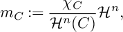 $$\begin{align*}m_C:=\frac{\chi_C}{\mathcal{H}^n(C)}\mathcal{H}^n, \end{align*}$$
where $\chi _C$
is the characteristic function of C and
$\chi _C$
is the characteristic function of C and $\mathcal {H}^n$
is the n-dimensional Hausdorff measure on
$\mathcal {H}^n$
is the n-dimensional Hausdorff measure on $\mathbb {R}^n$
. Of course
$\mathbb {R}^n$
. Of course $\mathcal {H}^n$
is equal to the n-dimensional Lebesgue measure
$\mathcal {H}^n$
is equal to the n-dimensional Lebesgue measure $\mathcal {L}^n$
, however, since we put on the field of view of collapsing phenomena of convex bodies into lower dimensional objects, we prefer to use the Hausdorff measure.
$\mathcal {L}^n$
, however, since we put on the field of view of collapsing phenomena of convex bodies into lower dimensional objects, we prefer to use the Hausdorff measure.
Definition 2.1.1. Define a function $d^W:\mathcal {C}_n\times \mathcal {C}_n\to \mathbb {R}_{\geq 0}$
by
$d^W:\mathcal {C}_n\times \mathcal {C}_n\to \mathbb {R}_{\geq 0}$
by
 $$\begin{align*}d^W(C_1, C_2):=W_2(m_{C_1}, m_{C_2}), \end{align*}$$
where $W_2$
is the
$W_2$
is the $L^2$
-Wasserstein distance on the set of all probability measures on
$L^2$
-Wasserstein distance on the set of all probability measures on $\mathbb {R}^n$
with finite quadratic moment.
$\mathbb {R}^n$
with finite quadratic moment.
See Appendix A for basic definitions and facts on $L^2$
-Wasserstein distance.
$L^2$
-Wasserstein distance.
Lemma 2.1.2. $d^W$
is a distance function on
$d^W$
is a distance function on $\mathcal {C}_n$
.
$\mathcal {C}_n$
.
Proof. Symmetricity, triangle inequality and non-negativity are clear. The non-degeneracy follows from the equivalence between the conditions $d^W(C_1, C_2)=W_2(m_{C_1}, m_{C_2})=0$
and
$d^W(C_1, C_2)=W_2(m_{C_1}, m_{C_2})=0$
and $C_1=\mathrm {supp}\,(m_{C_1})=\mathrm {supp}\,(m_{C_2})=C_2$
.
$C_1=\mathrm {supp}\,(m_{C_1})=\mathrm {supp}\,(m_{C_2})=C_2$
.
2.2 Lebesgue volume
For $C_1, C_2\in \mathcal {C}_n$
, let
$C_1, C_2\in \mathcal {C}_n$
, let $d^V(C_1, C_2)$
be the Lebesgue volume of the symmetric difference
$d^V(C_1, C_2)$
be the Lebesgue volume of the symmetric difference $C_1\bigtriangleup C_2:=(C_1\setminus C_2)\cup (C_2\setminus C_1)$
:
$C_1\bigtriangleup C_2:=(C_1\setminus C_2)\cup (C_2\setminus C_1)$
:
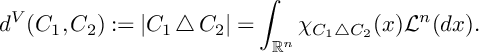 $$\begin{align*}d^V(C_1, C_2):=|C_1\bigtriangleup C_2|=\int_{\mathbb{R}^n}\chi_{C_1 \bigtriangleup C_2}(x)\mathcal{L}^n(dx). \end{align*}$$
This $d^V$
is indeed a distance function on
$d^V$
is indeed a distance function on $\mathcal {C}_n$
and used in a study of convex bodies classically. See [Reference Dinghas5] or [Reference Shephard and Webster15] for example.
$\mathcal {C}_n$
and used in a study of convex bodies classically. See [Reference Dinghas5] or [Reference Shephard and Webster15] for example.
2.3 Hausdorff distance
Let $d^H$
be the Hausdorff distance on the set of all compact subsets in
$d^H$
be the Hausdorff distance on the set of all compact subsets in $\mathbb {R}^n$
.We also denote the restriction of
$\mathbb {R}^n$
.We also denote the restriction of $d^H$
to
$d^H$
to $\mathcal {C}_n$
by the same letter
$\mathcal {C}_n$
by the same letter $d^H$
:
$d^H$
:
 $$\begin{align*}d^H(C_1, C_2):=\max\{\max_{x\in C_1}\min_{y\in C_2}\|x-y\|, \ \max_{y\in C_2}\min_{x\in C_1}\|x-y\| \} \quad (C_1, C_2\in \mathcal{C}_n). \end{align*}$$
3 Relation of distance functions
3.1 Equivalence among
$d^W$
,
$d^V$
, and
$d^H$


It is known that two distance functions $d^V$
and
$d^V$
and $d^H$
give the same metric topology. More precisely in [Reference Shephard and Webster15] it is shown that a sequence
$d^H$
give the same metric topology. More precisely in [Reference Shephard and Webster15] it is shown that a sequence $\{P_i\}_i$
in
$\{P_i\}_i$
in $\mathcal {C}_n$
converges to
$\mathcal {C}_n$
converges to $Q\in \mathcal {C}_n$
in
$Q\in \mathcal {C}_n$
in $d^V$
if and only if it converges to Q in
$d^V$
if and only if it converges to Q in $d^H$
.
$d^H$
.
Lemma 3.1.1. For a sequence $\{P_i\}_i$
in
$\{P_i\}_i$
in $\mathcal {C}_n$
and
$\mathcal {C}_n$
and $Q\in \mathcal {C}_n$
, if
$Q\in \mathcal {C}_n$
, if $d^V(P_i,Q)\to 0 \ (i\to \infty )$
, then we have
$d^V(P_i,Q)\to 0 \ (i\to \infty )$
, then we have $d^W(P_i ,Q)\to 0 \ (i\to \infty )$
.
$d^W(P_i ,Q)\to 0 \ (i\to \infty )$
.
Proof. Since $\displaystyle \lim _{i\to \infty }d^V(P_i, Q)=0$
implies
$\displaystyle \lim _{i\to \infty }d^V(P_i, Q)=0$
implies $\displaystyle \lim _{i\to \infty }d^H(P_i, Q)=0$
we may assume that
$\displaystyle \lim _{i\to \infty }d^H(P_i, Q)=0$
we may assume that $P_i\cap Q\neq \emptyset $
,
$P_i\cap Q\neq \emptyset $
,
 $$\begin{align*}K_i:=\operatorname{\mathrm{Diam}}(P_i)\leq 100K:=100\operatorname{\mathrm{Diam}}(Q), \end{align*}$$
and $|\log (|P_i|/|Q|)|<\epsilon $
for small
$|\log (|P_i|/|Q|)|<\epsilon $
for small $\epsilon>0$
and any i large enough.
$\epsilon>0$
and any i large enough.
If $\left \vert Q\right \vert \geq \left \vert P_i\right \vert $
, then we have
$\left \vert Q\right \vert \geq \left \vert P_i\right \vert $
, then we have $m_Q(Q\cap P_i)\leq m_{P_i}(Q\cap P_i)$
and define new probability measures
$m_Q(Q\cap P_i)\leq m_{P_i}(Q\cap P_i)$
and define new probability measures
 $$ \begin{align*} &\nu_0:=\frac{1}{m_Q(Q\setminus P_i)}m_Q\vert_{Q\setminus P_i},\\ &\nu_1:=\frac{1}{m_Q(Q\setminus P_i)}\left(m_{P_i}\vert_{P_i\setminus Q}+\left(1-\frac{m_Q(P_i\cap Q)}{m_{P_i}(P_i\cap Q)}\right)m_{P_i}\vert_{Q\cap P_i}\right). \end{align*} $$
Since $\nu _0,\nu _1\ll \mathcal {L}^n$
, by Theorem A.2.2, one can find a Borel map
$\nu _0,\nu _1\ll \mathcal {L}^n$
, by Theorem A.2.2, one can find a Borel map $T:\mathbb {R}^n\rightarrow \mathbb {R}^n$
with
$T:\mathbb {R}^n\rightarrow \mathbb {R}^n$
with $T_*\nu _0=\nu _1$
so that
$T_*\nu _0=\nu _1$
so that $W_2^2(\nu _0,\nu _1)=\int \left \Vert x-T(x)\right \Vert {}^2\,\nu _0(dx)$
. By using the map T, we define a coupling
$W_2^2(\nu _0,\nu _1)=\int \left \Vert x-T(x)\right \Vert {}^2\,\nu _0(dx)$
. By using the map T, we define a coupling $\xi _1\in \mathsf {Cpl}(m_Q,m_{P_i})$
by
$\xi _1\in \mathsf {Cpl}(m_Q,m_{P_i})$
by
 $$ \begin{align*} \xi_1:=(\mathsf{Id},T)_*m_Q\vert_{Q\setminus P_i}+(\mathsf{Id},\mathsf{Id})_*m_{Q}\vert_{Q\cap P_i}. \end{align*} $$
Heuristically, the coupling $\xi _1$
represents the transportation from
$\xi _1$
represents the transportation from $m_Q$
to
$m_Q$
to $m_{P_i}$
that
$m_{P_i}$
that
-
• the mass on
$Q\cap P_i$
measured by
$m_Q$
keep staying, and -
• the mass on
$Q\setminus P_i$
measured by
$m_Q$
distributes on
$P_i$
along the map T.


Note that since $\mathrm {supp}\,(T_*\nu _0)=\mathrm {supp}\,(\nu _1)\subset P_i$
, we have
$\mathrm {supp}\,(T_*\nu _0)=\mathrm {supp}\,(\nu _1)\subset P_i$
, we have $T(x)\in P_i$
for a.e.
$T(x)\in P_i$
for a.e. $x\in Q\setminus P_i$
. It also implies that
$x\in Q\setminus P_i$
. It also implies that $\|x-T(x)\|\leq \operatorname {\mathrm {Diam}} Q+\operatorname {\mathrm {Diam}} P_i\leq 101 K$
for a.e.
$\|x-T(x)\|\leq \operatorname {\mathrm {Diam}} Q+\operatorname {\mathrm {Diam}} P_i\leq 101 K$
for a.e. $x\in Q\setminus P_i$
, and hence, we have
$x\in Q\setminus P_i$
, and hence, we have
 $$\begin{align*}\int_{\mathbb{R}^n\times \mathbb{R}^n}\Vert x-y \Vert^2\xi_1(dx,dy) =\int_{\mathbb{R}^n}\|x-T(x)\|^2 m_Q|_{Q\setminus P_i}(dx) \leq \frac{\vert Q\setminus P_i\vert}{\vert Q\vert}\cdot (101 K)^2. \end{align*}$$
On the other hand, if $\left \vert P_i\right \vert \geq \left \vert Q\right \vert $
, then for two probability measures
$\left \vert P_i\right \vert \geq \left \vert Q\right \vert $
, then for two probability measures
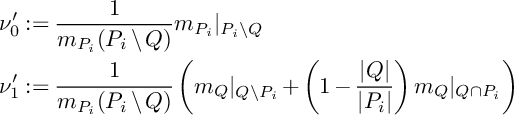 $$ \begin{align*} &\nu_0^{\prime}:=\frac{1}{m_{P_i}(P_i\setminus Q)}m_{P_i}\vert_{P_i\setminus Q} \\ &\nu_1^{\prime}:=\frac{1}{m_{P_i}(P_i\setminus Q)}\left(m_Q\vert_{Q\setminus P_i}+\left(1-\frac{\left\vert Q\right\vert}{\left\vert P_i\right\vert}\right)m_Q\vert_{Q\cap P_i}\right) \end{align*} $$
we can find a Borel map $S:\mathbb {R}^n\rightarrow \mathbb {R}^n$
with
$S:\mathbb {R}^n\rightarrow \mathbb {R}^n$
with $S_*\nu _0^{\prime }=\nu _1^{\prime }$
so that
$S_*\nu _0^{\prime }=\nu _1^{\prime }$
so that $W_2^2(\nu _0^{\prime },\nu _1^{\prime })=\int \left \Vert x-S(x)\right \Vert {}^2\nu _0^{\prime }(dx)$
. Then we have a coupling
$W_2^2(\nu _0^{\prime },\nu _1^{\prime })=\int \left \Vert x-S(x)\right \Vert {}^2\nu _0^{\prime }(dx)$
. Then we have a coupling $\xi _2\in \mathsf {Cpl}(\nu _0^{\prime },\nu _1^{\prime })$
by
$\xi _2\in \mathsf {Cpl}(\nu _0^{\prime },\nu _1^{\prime })$
by
 $$ \begin{align*} \xi_2:=(\mathsf{Id},S)_*m_{P_i}\vert_{P_i\setminus Q}+(\mathsf{Id},\mathsf{Id})_*m_{P_i}\vert_{Q\cap P_i}. \end{align*} $$
Then we have
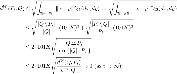 $$ \begin{align*} d^W(P_i,Q) &\leq \sqrt{\int_{\mathbb{R}^n\times \mathbb{R}^n}\Vert x-y \Vert^2\xi_1(dx,dy)} \ \mathrm{or} \ \sqrt{\int_{\mathbb{R}^n\times \mathbb{R}^n}\Vert x-y \Vert^2\xi_2(dx,dy)} \\ &\leq \sqrt{\frac{\vert Q\setminus P_i\vert}{\vert Q\vert}\cdot (101 K)^2}+\sqrt{\frac{\vert P_i\setminus Q\vert}{\vert P_i\vert}\cdot (101K)^2} \\ &\leq 2\cdot 101 K\sqrt{\frac{\vert Q\bigtriangleup P_i\vert}{\min\{\vert Q\vert,\vert P_i\vert\}}}\\ &\leq 2\cdot 101 K\sqrt{\frac{d^V(Q,P_i)}{e^{-\epsilon}\vert Q\vert}} \rightarrow 0 \ (\mathrm{as} \ i\to\infty).\\[-44pt] \end{align*} $$
Lemma 3.1.2. For a sequence $\{P_i\}_i$
in
$\{P_i\}_i$
in $\mathcal {C}_n$
and
$\mathcal {C}_n$
and $Q\in \mathcal {C}_n$
, if
$Q\in \mathcal {C}_n$
, if $d^W(P_i,Q)\to 0 \ (i\to \infty )$
, then we have
$d^W(P_i,Q)\to 0 \ (i\to \infty )$
, then we have $d^V(P_i ,Q)\to 0 \ (i\to \infty )$
.
$d^V(P_i ,Q)\to 0 \ (i\to \infty )$
.
Proof. Suppose that $d^W(P_i,Q)\to 0 \ (i\to \infty )$
. Then,
$d^W(P_i,Q)\to 0 \ (i\to \infty )$
. Then, $m_i:=m_{P_i}$
converges weakly to
$m_i:=m_{P_i}$
converges weakly to $m:=m_Q$
, in particular, we have
$m:=m_Q$
, in particular, we have
 $$\begin{align*}m_i(Q)=\frac{|P_i\cap Q|}{|P_i|}\to m(Q)=1 \end{align*}$$
by Theorem A.1.2. Since $|P_i\cap Q|\leq |Q|$
we have
$|P_i\cap Q|\leq |Q|$
we have $|P_i|$
is bounded, and hence,
$|P_i|$
is bounded, and hence,
 $$\begin{align*}\frac{|P_i|}{|Q|} <c \end{align*}$$
for some $c>0$
. Corollary A.2.3 implies that for two probability measures
$c>0$
. Corollary A.2.3 implies that for two probability measures $m_i$
and m there exist a sequence of Borel measurable maps
$m_i$
and m there exist a sequence of Borel measurable maps $\{T_i:\mathbb {R}^n\to \mathbb {R}^n\}_i$
such that
$\{T_i:\mathbb {R}^n\to \mathbb {R}^n\}_i$
such that $(\mathtt {id}\times T_i)_*m\in \mathsf {Opt}(m, m_i)$
for all i and
$(\mathtt {id}\times T_i)_*m\in \mathsf {Opt}(m, m_i)$
for all i and
 $$\begin{align*}m(\{x\in Q \ | \ \|x-T_i(x)\|\geq a\})=m(\{x\in \mathbb{R}^n \ | \ \|x-T_i(x)\|\geq a\}) \to 0 \ (i\to\infty) \end{align*}$$
for all $a>0$
. Let us fix an arbitrary positive number
$a>0$
. Let us fix an arbitrary positive number $\epsilon $
and set
$\epsilon $
and set
 $$\begin{align*}\xi:= \frac{\epsilon}{(c+1)(|Q|+1)}. \end{align*}$$
Choose $\eta $
small enough so that
$\eta $
small enough so that
 $$\begin{align*}|B(Q,\eta)\setminus Q|< \xi. \end{align*}$$
There exists $N\in \mathbb {N}$
such that
$N\in \mathbb {N}$
such that
 $$\begin{align*}m(\{x\in Q \ | \ \|T_i(x)-x\|\geq \eta\})<\xi \end{align*}$$
for all $i \geq N$
. Take and fix
$i \geq N$
. Take and fix $i> N$
. For
$i> N$
. For $x\in Q$
we put
$x\in Q$
we put $r_x^i:=\|x-T_i(x)\|$
. Then we have
$r_x^i:=\|x-T_i(x)\|$
. Then we have $\displaystyle Q\subset \bigcup _{x\in Q}B(x, r_x^i)$
. We put
$\displaystyle Q\subset \bigcup _{x\in Q}B(x, r_x^i)$
. We put
 $$\begin{align*}U^i:=\bigcup_{x\in Q, r_x^i\leq \eta}\overline{B(x, r_x^i)}. \end{align*}$$
We have
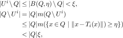 $$ \begin{align*} |U^i\setminus Q|&\leq |B(Q,\eta)\setminus Q|<\xi, \\ |Q\setminus U^i|&=|Q| m(Q\setminus U^i) \\ &\leq |Q| m(\{x\in Q \ | \ \|x-T_i(x)\|)\geq\eta\}) \\ &<|Q|\xi , \end{align*} $$
and hence, $|Q\bigtriangleup U^i|<(|Q|+1)\xi $
. On the other hand we have
$|Q\bigtriangleup U^i|<(|Q|+1)\xi $
. On the other hand we have
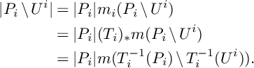 $$ \begin{align*} |P_i\setminus U^i|&=|P_i|m_i(P_i\setminus U^i) \\ &= |P_i|(T_i)_*m(P_i\setminus U^i) \\ &= |P_i| m(T_i^{-1}(P_i)\setminus T_i^{-1}(U^i)). \end{align*} $$
Since $(T_i)_*m=m_i$
we have that
$(T_i)_*m=m_i$
we have that $T_i^{-1}(P_i)=Q$
(m-a.e.). This fact and
$T_i^{-1}(P_i)=Q$
(m-a.e.). This fact and $T_i^{-1}(\overline {B(x,r_x^i)})\ni x$
imply that
$T_i^{-1}(\overline {B(x,r_x^i)})\ni x$
imply that
 $$\begin{align*}T_i^{-1}(U^i)\supset \{x\in Q \ | \ \|x-T_i(x)\|\leq \eta\}. \end{align*}$$
In particular we have
 $$\begin{align*}|P_i\setminus U^i|\leq |P_i| m(\{x\in Q \ | \ \|x-T_i(x)\|>\eta\})\leq |P_i|\xi. \end{align*}$$
Similarly we have
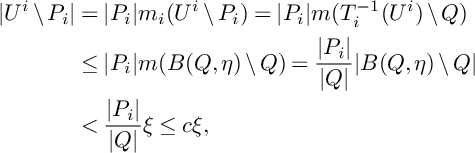 $$ \begin{align*} \vert U^i\setminus P_i\vert&=\vert P_i\vert m_i(U^i\setminus P_i)=\vert P_i\vert m(T_i^{-1}(U^i)\setminus Q)\\ &\leq\vert P_i\vert m(B(Q,\eta)\setminus Q)=\frac{\vert P_i\vert}{\vert Q\vert}\vert B(Q,\eta)\setminus Q\vert\\ &<\frac{\vert P_i\vert}{\vert Q\vert}\xi\leq c\xi, \end{align*} $$
and hence $\vert U^i\bigtriangleup P_i\vert \leq (\vert P_i\vert +c)\xi $
. Therefore we have
$\vert U^i\bigtriangleup P_i\vert \leq (\vert P_i\vert +c)\xi $
. Therefore we have
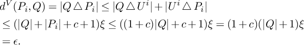 $$ \begin{align*} &d^V(P_i,Q)=\vert Q\bigtriangleup P_i\vert\leq \vert Q\bigtriangleup U^i\vert+\vert U^i\bigtriangleup P_i\vert\\ &\leq (\vert Q\vert+\vert P_i\vert+c+1)\xi\leq ((1+c)\vert Q\vert+c+1)\xi=(1+c)(\vert Q\vert+1)\xi\\ &=\epsilon. \end{align*} $$
Since $\epsilon> 0$
is arbitrary, we obtain the conclusion, that is,
$\epsilon> 0$
is arbitrary, we obtain the conclusion, that is, $d^V(P_i,Q)\rightarrow 0$
.
$d^V(P_i,Q)\rightarrow 0$
.
As a corollary of Lemmas 3.1.1 and 3.1.2 we have the following by Kratowski’s axiom and the coincidence between the metric topology of $d^V$
and
$d^V$
and $d^H$
as shown in [Reference Shephard and Webster15].
$d^H$
as shown in [Reference Shephard and Webster15].
Theorem 3.1.3. Three metric topologies on $\mathcal {C}_n$
determined by
$\mathcal {C}_n$
determined by $d^W$
,
$d^W$
, $d^V$
, and
$d^V$
, and $d^H$
coincide with each other.
$d^H$
coincide with each other.
3.2 Moduli space of convex bodies and its topology
We introduce the moduli space of convex bodies following [Reference Fujita and Ohashi6] and [Reference Pelayo, Pires, Ratiu and Sabatini14]. Let $G_n:=\mathrm {AGL}(n,\mathbb {Z})$
be the integral affine transformation group. Namely
$G_n:=\mathrm {AGL}(n,\mathbb {Z})$
be the integral affine transformation group. Namely $G_n$
is the direct product
$G_n$
is the direct product $\mathrm {GL}(n,\mathbb {Z})\times \mathbb {R}^n$
as a set and the multiplication on
$\mathrm {GL}(n,\mathbb {Z})\times \mathbb {R}^n$
as a set and the multiplication on $G_n$
is defined by
$G_n$
is defined by
 $$\begin{align*}(A_1, t_1)\cdot(A_2, t_2):=(A_1A_2, A_1t_2+t_1) \end{align*}$$
for each $(A_1, t_1), (A_2, t_2)\in G_n$
. This group
$(A_1, t_1), (A_2, t_2)\in G_n$
. This group $G_n$
acts on
$G_n$
acts on $\mathcal {C}_n$
in a natural way, and
$\mathcal {C}_n$
in a natural way, and $C\in \mathcal {C}_n$
and
$C\in \mathcal {C}_n$
and $C'\in \mathcal {C}_n$
are called
$C'\in \mathcal {C}_n$
are called $G_n$
-congruent if C and
$G_n$
-congruent if C and $C'$
are contained in the same
$C'$
are contained in the same $G_n$
-orbit.
$G_n$
-orbit.
Definition 3.2.1. The moduli space of convex bodies $\widetilde {\mathcal {C}}_n$
with respect to the
$\widetilde {\mathcal {C}}_n$
with respect to the $G_n$
-congruence is defined by the quotient
$G_n$
-congruence is defined by the quotient
 $$\begin{align*}\widetilde{\mathcal{C}}_n:=\mathcal{C}_n/G_n. \end{align*}$$
Let $\pi $
be the natural projection from
$\pi $
be the natural projection from $\mathcal {C}_n$
to
$\mathcal {C}_n$
to $\widetilde {\mathcal {C}}_n$
.
$\widetilde {\mathcal {C}}_n$
.
Definition 3.2.2. Define a function $D^V:\widetilde {\mathcal {C}}_n\times \widetilde {\mathcal {C}}_n\to \mathbb {R}$
by
$D^V:\widetilde {\mathcal {C}}_n\times \widetilde {\mathcal {C}}_n\to \mathbb {R}$
by
 $$\begin{align*}D^V(\alpha, \beta):=\inf\{d^V(P_1, P_2) \ | \ \pi(P_1)=\alpha, \pi(P_2)=\beta\} \end{align*}$$
for $(\alpha , \beta )\in \widetilde {\mathcal {C}}_n\times \widetilde {\mathcal {C}}_n$
.
$(\alpha , \beta )\in \widetilde {\mathcal {C}}_n\times \widetilde {\mathcal {C}}_n$
.
Theorem 3.2.3 [Reference Fujita and Ohashi6]. $D^V$
is a distance function on
$D^V$
is a distance function on $\widetilde {\mathcal {C}}_n$
and its metric topology coincides with the quotient topology induced from
$\widetilde {\mathcal {C}}_n$
and its metric topology coincides with the quotient topology induced from $\pi $
.
$\pi $
.
This $G_n$
-action and the moduli space
$G_n$
-action and the moduli space $\widetilde {\mathcal {C}}_n$
arise naturally in the context of the geometry of symplectic toric manifolds. In the subsequent sections we will discuss from such point of view.
$\widetilde {\mathcal {C}}_n$
arise naturally in the context of the geometry of symplectic toric manifolds. In the subsequent sections we will discuss from such point of view.
Remark 3.2.4. As it is noted in [Reference Fujita and Ohashi6] we can not define a distance function on $\widetilde {\mathcal {C}}_n$
by using the infimum of
$\widetilde {\mathcal {C}}_n$
by using the infimum of $d^H$
(or
$d^H$
(or $d^W$
) among all representatives, though, one may hope that by considering infimum of
$d^W$
) among all representatives, though, one may hope that by considering infimum of $d^H$
among only “standard”representatives we can define a distance function on
$d^H$
among only “standard”representatives we can define a distance function on $\widetilde {\mathcal {C}}_n$
. One possible candidates of “standard”representatives are the minimum variance (or quadratic moment) elements in the following sense.
$\widetilde {\mathcal {C}}_n$
. One possible candidates of “standard”representatives are the minimum variance (or quadratic moment) elements in the following sense.
For each $C\in \mathcal {C}_n$
define its variance by
$C\in \mathcal {C}_n$
define its variance by
 $$\begin{align*}\mathsf{Var}(C):=\frac{1}{|C|}\int_C\|x-\mathsf{b}(C)\|^2\mathcal{L}^n(dx), \end{align*}$$
where $\mathsf {b}(C)$
is the barycenter of C which is determined uniquely by the condition
$\mathsf {b}(C)$
is the barycenter of C which is determined uniquely by the condition
 $$\begin{align*}\langle \mathsf{b}(C), y \rangle =\int_{\mathbb{R}^n}\langle x, y \rangle \mathcal{L}^n(dx) \end{align*}$$
for any $y\in \mathbb {R}^n$
. See [Reference Sturm17] for example. The minimum variance element
$y\in \mathbb {R}^n$
. See [Reference Sturm17] for example. The minimum variance element $C\in \mathcal {C}_n$
is an element of
$C\in \mathcal {C}_n$
is an element of
 $$\begin{align*}\mathsf{argmin}\left\{ \mathsf{Var}(C') \ | \ C'\in\mathcal{C}_n \ \mathrm{is} \ G_n \text{-congruent to} \ C\right\}. \end{align*}$$
One can see that for any $C\in \mathcal {C}_n$
there exist at least one and finitely many minimum variance elements which have the common barycenter are
$C\in \mathcal {C}_n$
there exist at least one and finitely many minimum variance elements which have the common barycenter are $G_n$
-congruent to C.
$G_n$
-congruent to C.
4 Delzant polytopes and symplectic toric manifolds.
4.1 Delzant polytopes, symplectic toric manifolds and their moduli space
Definition 4.1.1. A convex polytope P in $\mathbb {R}^n$
is called a Delzant polytope if P satisfies the following conditions:
$\mathbb {R}^n$
is called a Delzant polytope if P satisfies the following conditions:
-
• P is simple, that is, each vertex of P has exactly n edges.
-
• P is rational, that is, at each vertex all directional vectors of edges can be taken as integral vectors in
$\mathbb {Z}^n$
. -
• P is smooth, that is, at each vertex we can take integral directional vectors of edges as a
$\mathbb {Z}$
-basis of
$\mathbb {Z}^n$
in
$\mathbb {R}^n$
.


We denote the subset of $\mathcal {C}_n$
consisting of all Delzant polytopes by
$\mathcal {C}_n$
consisting of all Delzant polytopes by $\mathcal {D}_n$
and define their moduli space by
$\mathcal {D}_n$
and define their moduli space by $\widetilde {\mathcal {D}}_n:=\mathcal {D}_n/G_n$
.
$\widetilde {\mathcal {D}}_n:=\mathcal {D}_n/G_n$
.
Recall that the data of a (compact) symplectic toric manifold $(M,\omega , \rho , \mu )$
consists of
$(M,\omega , \rho , \mu )$
consists of
-
• a compact connected symplectic manifold
$(M,\omega )$
of dimension
$2n$
, -
• a homomorphism
$\rho $
from the n-dimensional torus
$T^n$
to the group of symplectomorphisms of M which gives a Hamiltonian action of
$T^n$
on M and -
• a moment map
$\mu :M\to \mathbb {R}^n=(\mathrm {Lie}(T^n))^*$
.


The famous Delzant construction gives a correspondence between Delzant polytopes and symplectic toric manifolds.
Theorem 4.1.2 [Reference Karshon, Kessler and Pinsonnault12].
The Delzant construction gives a bijective correspondence between $\widetilde {\mathcal {D}}_n$
and the set of all weak isomorphism classes of
$\widetilde {\mathcal {D}}_n$
and the set of all weak isomorphism classes of $2n$
-dimensional symplectic toric manifolds.
$2n$
-dimensional symplectic toric manifolds.
Here two symplectic toric manifolds $(M_1, \omega _1, \rho _1,\mu _1)$
and
$(M_1, \omega _1, \rho _1,\mu _1)$
and $(M_2, \omega _2, \rho _2, \mu _2)$
are weakly isomorphic
Footnote
1
if there exist a diffeomorphism
$(M_2, \omega _2, \rho _2, \mu _2)$
are weakly isomorphic
Footnote
1
if there exist a diffeomorphism $f:M_1\to M_2$
and a group isomorphism
$f:M_1\to M_2$
and a group isomorphism $\phi :T^n\to T^n$
such that
$\phi :T^n\to T^n$
such that
 $$\begin{align*}f^*\omega_2=\omega_1 \ \mathrm{and} \ \rho_1(g)(x)=\rho_2(\phi(g))(f(x)) \ \mathrm{for\ all } \ (g,x)\in T^n\times M_1. \end{align*}$$
Based on the above fact the moduli space $\widetilde {\mathcal {D}}_n$
is also called the moduli space of toric manifolds in [Reference Pelayo, Pires, Ratiu and Sabatini14]. In [Reference Pelayo, Pires, Ratiu and Sabatini14] they show that
$\widetilde {\mathcal {D}}_n$
is also called the moduli space of toric manifolds in [Reference Pelayo, Pires, Ratiu and Sabatini14]. In [Reference Pelayo, Pires, Ratiu and Sabatini14] they show that $(\mathcal {D}_n,d^V)$
is neither complete nor locally compact and
$(\mathcal {D}_n,d^V)$
is neither complete nor locally compact and $\widetilde {\mathcal {D}}_2$
is path connected.
$\widetilde {\mathcal {D}}_2$
is path connected.
4.2 Brief review on the Delzant construction
For later convenience we give a brief review on the Delzant construction here.
Let P be an n-dimensional Delzant polytope and
 $$ \begin{align} l^{(r)}(x):=\langle x, \nu^{(r)}\rangle - \lambda^{(r)}=0 \quad (r=1,\ldots, N) \end{align} $$
a system of defining affine equations on $\mathbb {R}^n$
of facets of P, each
$\mathbb {R}^n$
of facets of P, each $\nu ^{(r)}$
being inward pointing normal vector of rth facet and N is the number of facets of P. In other words P can be described as
$\nu ^{(r)}$
being inward pointing normal vector of rth facet and N is the number of facets of P. In other words P can be described as
 $$\begin{align*}P=\bigcap_{r=1}^N\{x\in\mathbb{R}^n \ | \ l^{(r)}(x)\geq 0\}, \end{align*}$$
and we do not allow redundant inequalities. We may assume that each $\nu ^{(r)}$
is primitiveFootnote
2
and they form a
$\nu ^{(r)}$
is primitiveFootnote
2
and they form a $\mathbb {Z}$
-basis of
$\mathbb {Z}$
-basis of $\mathbb {Z}^n$
. Consider the standard Hamiltonian action of the N-dimensional torus
$\mathbb {Z}^n$
. Consider the standard Hamiltonian action of the N-dimensional torus $T^N$
on
$T^N$
on $\mathbb {C}^N$
with the moment map
$\mathbb {C}^N$
with the moment map
 $$\begin{align*}\tilde\mu:\mathbb{C}^N\to (\mathbb{R}^N)^*=\mathrm{Lie}(T^N)^*, \ (z_1, \ldots, z_N)\mapsto -\frac{1}{2}(|z_1|^2, \ldots, |z_N|^2)+(\lambda^{(1)}, \ldots, \lambda^{(N)}). \end{align*}$$
Let $\tilde \pi :\mathbb {R}^N\to \mathbb {R}^n$
be the linear map defined by
$\tilde \pi :\mathbb {R}^N\to \mathbb {R}^n$
be the linear map defined by $e_r\mapsto \nu ^{(r)}$
, where
$e_r\mapsto \nu ^{(r)}$
, where $e_r$
(
$e_r$
( $r=1,\ldots , N$
) is the rth standard basis of
$r=1,\ldots , N$
) is the rth standard basis of $\mathbb {R}^N$
. Note that
$\mathbb {R}^N$
. Note that $\tilde \pi $
induces a surjection
$\tilde \pi $
induces a surjection $\tilde \pi :\mathbb {Z}^N\to \mathbb {Z}^n$
between the standard lattices by the last condition in Definition 4.1.1, and hence it induces a surjective homomorphism between tori, still denoted by
$\tilde \pi :\mathbb {Z}^N\to \mathbb {Z}^n$
between the standard lattices by the last condition in Definition 4.1.1, and hence it induces a surjective homomorphism between tori, still denoted by $\tilde \pi $
,
$\tilde \pi $
,
 $$\begin{align*}\tilde\pi:T^N=\mathbb{R}^N/\mathbb{Z}^N\to T^n=\mathbb{R}^n/\mathbb{Z}^n. \end{align*}$$
Let H be the kernel of $\tilde \pi $
which is an
$\tilde \pi $
which is an $(N-n)$
-dimensional subtorus of
$(N-n)$
-dimensional subtorus of $T^N$
and
$T^N$
and $\mathfrak {h}$
its Lie algebra. We have exact sequences
$\mathfrak {h}$
its Lie algebra. We have exact sequences
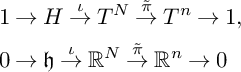 $$\begin{align*}1&\to H\stackrel{\iota}{\to} T^N\stackrel{\tilde\pi}{\to} T^n\to 1,\\0 &\to \mathfrak{h}\stackrel{\iota}{\to} \mathbb{R}^N\stackrel{\tilde\pi}{\to} \mathbb{R}^n\to 0 \end{align*}$$
and its dual
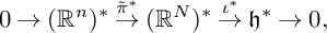 $$\begin{align*}0 \to (\mathbb{R}^n)^* \stackrel{\tilde\pi^*}{\to} (\mathbb{R}^N)^*\stackrel{\iota^*}{\to} \mathfrak{h}^*\to 0, \end{align*}$$
where $\iota $
is the inclusion map. Then the composition
$\iota $
is the inclusion map. Then the composition $\iota ^*\circ \tilde \mu :\mathbb {C}^N\to \mathfrak {h}^*$
is the associated moment map of the action of H on
$\iota ^*\circ \tilde \mu :\mathbb {C}^N\to \mathfrak {h}^*$
is the associated moment map of the action of H on $\mathbb {C}^N$
. It is known that
$\mathbb {C}^N$
. It is known that $(\iota ^*\circ \tilde \mu )^{-1}(0)$
is a compact submanifold of
$(\iota ^*\circ \tilde \mu )^{-1}(0)$
is a compact submanifold of $\mathbb {C}^N$
and H acts freely on it. We obtain the desired symplectic manifold
$\mathbb {C}^N$
and H acts freely on it. We obtain the desired symplectic manifold $M_P:=(\iota ^*\circ \tilde \mu )^{-1}(0)/H$
equipped with a natural Hamiltonian
$M_P:=(\iota ^*\circ \tilde \mu )^{-1}(0)/H$
equipped with a natural Hamiltonian $T^N/H=T^n$
-action. Note that the standard flat Kähler structure on
$T^N/H=T^n$
-action. Note that the standard flat Kähler structure on $\mathbb {C}^N$
induces a Kähler structure on
$\mathbb {C}^N$
induces a Kähler structure on $M_P$
Footnote
3
. We call the associated Riemannian metric the Guillemin metric.
$M_P$
Footnote
3
. We call the associated Riemannian metric the Guillemin metric.
There exists an explicit description of the Guillemin metric. We give the description following [Reference Abreu1]. Consider a smooth function
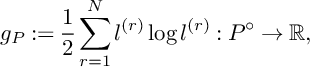 $$ \begin{align} g_P:=\frac{1}{2}\sum_{r=1}^Nl^{(r)}\log l^{(r)} : P^{\circ}\to \mathbb{R}, \end{align} $$
where $P^{\circ }$
is the interior of P. It is known that
$P^{\circ }$
is the interior of P. It is known that $M_P^{\circ }:=\mu _P^{-1}(P^{\circ })$
is an open dense subset of
$M_P^{\circ }:=\mu _P^{-1}(P^{\circ })$
is an open dense subset of $M_P$
on which
$M_P$
on which $T^n$
acts freely and there exists a diffeomorphism
$T^n$
acts freely and there exists a diffeomorphism $M_P^{\circ }\cong P^{\circ }\times T^n$
. Under this identification
$M_P^{\circ }\cong P^{\circ }\times T^n$
. Under this identification $\omega _P|_{M_P^{\circ }}$
can be described as
$\omega _P|_{M_P^{\circ }}$
can be described as
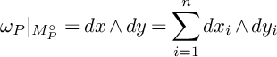 $$\begin{align*}\omega_P|_{M_P^{\circ}}=dx\wedge dy=\sum_{i=1}^ndx_i\wedge dy_i \end{align*}$$
using the standard coordinateFootnote
4 $(x,y)=(x_1, \ldots , x_n, y_1, \ldots , y_n)\in P^{\circ }\times T^n$
. The coordinate on
$(x,y)=(x_1, \ldots , x_n, y_1, \ldots , y_n)\in P^{\circ }\times T^n$
. The coordinate on $M_P^{\circ }$
induced from
$M_P^{\circ }$
induced from $(x,y)\in P^{\circ }\times T^n$
is called the symplectic coordinate on
$(x,y)\in P^{\circ }\times T^n$
is called the symplectic coordinate on $M_{P}$
.
$M_{P}$
.
Theorem 4.2.1 [Reference Guillemin9].
Under the symplectic coordinates $(x,y)\in P^{\circ }\times T^n\cong M_P^{\circ }\subset M_P$
, the Guillemin metric can be described as
$(x,y)\in P^{\circ }\times T^n\cong M_P^{\circ }\subset M_P$
, the Guillemin metric can be described as
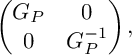 $$\begin{align*}\begin{pmatrix} G_P & 0 \\ 0 & G_P^{-1} \end{pmatrix}, \end{align*}$$
where $\displaystyle G_P:=\mathrm {Hess}_x(g_P)=\left (\frac {\partial ^2 g_P}{\partial x_k\partial x_l}\right )_{k,l=1,\ldots , n}$
is the Hessian of
$\displaystyle G_P:=\mathrm {Hess}_x(g_P)=\left (\frac {\partial ^2 g_P}{\partial x_k\partial x_l}\right )_{k,l=1,\ldots , n}$
is the Hessian of $g_P$
.
$g_P$
.
Remark 4.2.2. If P and $P'$
in
$P'$
in $\mathcal {D}_n$
are
$\mathcal {D}_n$
are $G_n$
-congruent, then the corresponding Riemannian manifolds
$G_n$
-congruent, then the corresponding Riemannian manifolds $M_P$
and
$M_P$
and $M_{P'}$
are isometric to each other. In fact as it is noted in [Reference Abreu1, Section 3.3], for
$M_{P'}$
are isometric to each other. In fact as it is noted in [Reference Abreu1, Section 3.3], for $\varphi \in G_n$
we have an isomorphism between
$\varphi \in G_n$
we have an isomorphism between $M_P$
and
$M_P$
and $M_{\varphi (P)}$
as Kähler manifolds. The isomorphism is induced by the map
$M_{\varphi (P)}$
as Kähler manifolds. The isomorphism is induced by the map $P\times T\to \varphi (P)\times T$
,
$P\times T\to \varphi (P)\times T$
, $(x,t)\mapsto (\varphi (x), ((\varphi _*)^{-1})^{T}(t))$
, where
$(x,t)\mapsto (\varphi (x), ((\varphi _*)^{-1})^{T}(t))$
, where $(\ )^{T}$
is the transpose and
$(\ )^{T}$
is the transpose and $\varphi _*$
is the automorphism of T which is induced by
$\varphi _*$
is the automorphism of T which is induced by $\varphi $
.
$\varphi $
.
Example 4.2.3. We demonstrate the Delzant construction in dimension $1$
. For
$1$
. For $\alpha \geq 1$
consider the inequalities
$\alpha \geq 1$
consider the inequalities
 $$\begin{align*}\xi \geq 0, \ 2\alpha-\xi\geq 0 \end{align*}$$
on ${\mathbb R}$
. These inequalities determine a 1-dimensional Delzant polytope
${\mathbb R}$
. These inequalities determine a 1-dimensional Delzant polytope $P_\alpha =[0,2\alpha ]$
.
$P_\alpha =[0,2\alpha ]$
.
Let $\tilde \mu :{\mathbb C}^2\to {\mathbb R}^2$
be the moment map defined by
$\tilde \mu :{\mathbb C}^2\to {\mathbb R}^2$
be the moment map defined by
 $$\begin{align*}\tilde\mu(z_1, z_2):=\left(-\frac{1}{2}|z_1|^2, -\frac{1}{2}|z_2|^2+2\alpha\right). \end{align*}$$
The inequalities determines a linear map $\tilde \pi :{\mathbb R}^2\to {\mathbb R}$
defined by
$\tilde \pi :{\mathbb R}^2\to {\mathbb R}$
defined by
 $$\begin{align*}\tilde\pi(e_1)=1, \ \tilde\pi(e_2)=-1. \end{align*}$$
Let H be the kernel of the induced homomorphism $\tilde \pi :T^2\to T^1$
, which is given by
$\tilde \pi :T^2\to T^1$
, which is given by
 $$\begin{align*}H=\{(t, t)\in T^2 \ | \ t\in U(1)\}\cong S^1. \end{align*}$$
Let $\mu _H:{\mathbb C}^2\to (\mathrm {Lie}(H))^*\cong {\mathbb R}$
be the induced moment map with respect to the H-action, which is given by
$\mu _H:{\mathbb C}^2\to (\mathrm {Lie}(H))^*\cong {\mathbb R}$
be the induced moment map with respect to the H-action, which is given by
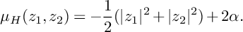 $$\begin{align*}\mu_H(z_1, z_2)=-\frac{1}{2}(|z_1|^2+|z_2|^2)+2\alpha. \end{align*}$$
One can see that $0\in {\mathbb R}$
is a regular value of
$0\in {\mathbb R}$
is a regular value of $\mu _H$
and the induced action of H on
$\mu _H$
and the induced action of H on $Z:=\mu _H^{-1}(0)$
is free, and hence, the quotient
$Z:=\mu _H^{-1}(0)$
is free, and hence, the quotient $M_\alpha :=\mu _H^{-1}(0)/H$
has a structure of compact 2-dimensional symplectic manifold equipped with Hamiltonian
$M_\alpha :=\mu _H^{-1}(0)/H$
has a structure of compact 2-dimensional symplectic manifold equipped with Hamiltonian $T:=T^2/H\cong S^1$
-action.
$T:=T^2/H\cong S^1$
-action.
On the other hand the Hessian of the function
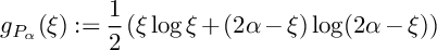 $$\begin{align*}g_{P_\alpha}(\xi):=\frac{1}{2}\left(\xi\log\xi+(2\alpha-\xi)\log(2\alpha-\xi)\right) \end{align*}$$
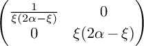
gives the Guillemin metric described as
 $$\begin{align*}\begin{pmatrix} \frac{1}{\xi(2\alpha-\xi)} & 0 \\ 0 & \xi(2\alpha-\xi) \end{pmatrix} \end{align*}$$
on $P_\alpha ^\circ \times T$
. By the direct computation we have that the (Gauss) curvature of this metric is constant
$P_\alpha ^\circ \times T$
. By the direct computation we have that the (Gauss) curvature of this metric is constant $\frac {1}{\alpha }$
. It turns out that M is isomorphic to the unit sphere with the standard
$\frac {1}{\alpha }$
. It turns out that M is isomorphic to the unit sphere with the standard $S^1$
-action and the round metric.
$S^1$
-action and the round metric.
By taking the limit $\alpha \to 1$
, we see that
$\alpha \to 1$
, we see that $P_\alpha $
converges to
$P_\alpha $
converges to $P_1=[0,2]$
. On the other hand the curvature of
$P_1=[0,2]$
. On the other hand the curvature of $M_\alpha $
converges to the constant
$M_\alpha $
converges to the constant $1$
. In fact by Theorem 5.2.2
$1$
. In fact by Theorem 5.2.2 $M_\alpha $
converges to the unit sphere
$M_\alpha $
converges to the unit sphere $M_1$
in the T-equivariant Gromov–Hausdorff topology.
$M_1$
in the T-equivariant Gromov–Hausdorff topology.
5 Convergence of polytopes and symplectic toric manifolds
Hereafter we do not often distinguish a sequence itself and a subsequence of it.
5.1 Convergence of polytopes and related quantities
For a convex polytope P in $\mathbb {R}^n$
let
$\mathbb {R}^n$
let $N_k(P)$
be the number of k-dimensional faces of P. We denote the set of all k-dimensional faces of P by
$N_k(P)$
be the number of k-dimensional faces of P. We denote the set of all k-dimensional faces of P by
 $$\begin{align*}\{F_{k}^{(r)}(P) \ | \ r\}=\{F_{k}^{(r)}(P) \ | \ r=1, \ldots, N_k(P)\}. \end{align*}$$
We often omit the superscript r for simplicity and denote each face by $F_k(P)$
for example.
$F_k(P)$
for example.
Remark 5.1.1. Since the Hausdorff distance between two convex bodies is equal to that between the boundaries of them, the following holds :
For a sequence $\{P_i\}_i\subset \mathcal {D}_n$
suppose that
$\{P_i\}_i\subset \mathcal {D}_n$
suppose that $d^H(P_i, P)\to 0 \ (i\to \infty )$
for
$d^H(P_i, P)\to 0 \ (i\to \infty )$
for $P\in \mathcal {D}_n$
. Then for any
$P\in \mathcal {D}_n$
. Then for any $x\in F_{n-1}^{(r)}(P)$
there exists a sequence
$x\in F_{n-1}^{(r)}(P)$
there exists a sequence $\{x_i\in F_{n-1}^{(r_i)}(P_i)\}_i$
such that
$\{x_i\in F_{n-1}^{(r_i)}(P_i)\}_i$
such that $x_i\to x \ (i\to \infty )$
.
$x_i\to x \ (i\to \infty )$
.
This fact implies the following corollaries.
Corollary 5.1.2. For a sequence $\{P_i\}_i\subset \mathcal {D}_n$
suppose that
$\{P_i\}_i\subset \mathcal {D}_n$
suppose that $d^H(P_i, P)\to 0 \ (i\to \infty )$
for
$d^H(P_i, P)\to 0 \ (i\to \infty )$
for $P\in \mathcal {D}_n$
. For any
$P\in \mathcal {D}_n$
. For any $k=0,1,\ldots , n-1$
and a point
$k=0,1,\ldots , n-1$
and a point $x\in F_{k}^{(r)}(P)$
there exists a sequence
$x\in F_{k}^{(r)}(P)$
there exists a sequence $\{x_i\in F_{k}^{(r_i)}(P_i)\}_i$
such that
$\{x_i\in F_{k}^{(r_i)}(P_i)\}_i$
such that $x_i \to x \ (i\to \infty )$
.
$x_i \to x \ (i\to \infty )$
.
Proof. For any $x\in F_{n-2}^{(r)}(P)$
let
$x\in F_{n-2}^{(r)}(P)$
let $F_{n-1}^{(r')}(P)$
be a facet of P which contains
$F_{n-1}^{(r')}(P)$
be a facet of P which contains $x\in F_{n-2}^{(r)}(P)$
. By the fact in Remark 5.1.1
$x\in F_{n-2}^{(r)}(P)$
. By the fact in Remark 5.1.1 $F_{n-1}^{(r')}(P)$
can be described as a limit of a union of facets of
$F_{n-1}^{(r')}(P)$
can be described as a limit of a union of facets of $P_i$
. It also implies that
$P_i$
. It also implies that $F_{n-2}^{(r)}(P)$
can be described as a limit of
$F_{n-2}^{(r)}(P)$
can be described as a limit of $(n-2)$
-dimensional faces of
$(n-2)$
-dimensional faces of $P_i$
. One can prove the claim in an inductive way.
$P_i$
. One can prove the claim in an inductive way.
Corollary 5.1.3. For a sequence $\{P_i\}_i\subset \mathcal {D}_n$
suppose that
$\{P_i\}_i\subset \mathcal {D}_n$
suppose that $d^H(P_i, P)\to 0 \ (i\to \infty )$
for
$d^H(P_i, P)\to 0 \ (i\to \infty )$
for $P\in \mathcal {D}_n$
. Then the number of k-dimensional faces is lower semi-continuous for any k:
$P\in \mathcal {D}_n$
. Then the number of k-dimensional faces is lower semi-continuous for any k:
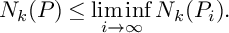 $$\begin{align*}N_k(P)\leq\liminf_{i\to\infty} N_k(P_i). \end{align*}$$
Corollary 5.1.4. For a sequence $\{P_i\}_i\subset \mathcal {D}_n$
suppose that
$\{P_i\}_i\subset \mathcal {D}_n$
suppose that $d^H(P_i, P)\to 0 \ (i\to \infty )$
for
$d^H(P_i, P)\to 0 \ (i\to \infty )$
for $P\in \mathcal {D}_n$
. For any facet
$P\in \mathcal {D}_n$
. For any facet $F_{n-1}^{(r)}(P)$
there exists a sequence of facets
$F_{n-1}^{(r)}(P)$
there exists a sequence of facets $\{F^{(r_i)}_{n-1}(P_{i})\}_i$
such that the corresponding defining affine functions converge to that of
$\{F^{(r_i)}_{n-1}(P_{i})\}_i$
such that the corresponding defining affine functions converge to that of $F_{n-1}^{(r)}(P)$
, that is,
$F_{n-1}^{(r)}(P)$
, that is, $l_{i}^{(r_i)}\to l^{(r)} (i\to \infty )$
.
$l_{i}^{(r_i)}\to l^{(r)} (i\to \infty )$
.
Proof. For any $x\in F^{(r)}_{n-1}(P)$
of P, one can take a sequence
$x\in F^{(r)}_{n-1}(P)$
of P, one can take a sequence $\{x_i\in F^{(r_i)}_{n-1}(P_i)\}_i$
of
$\{x_i\in F^{(r_i)}_{n-1}(P_i)\}_i$
of $P_i$
which converges to x. We may assume that the sequence of unit normal vectors of
$P_i$
which converges to x. We may assume that the sequence of unit normal vectors of $F^{(r_i)}_{n-1}(P_i)$
converges to that of
$F^{(r_i)}_{n-1}(P_i)$
converges to that of $F^{(r)}_{n-1}(P)$
. It implies that the corresponding defining affine functions
$F^{(r)}_{n-1}(P)$
. It implies that the corresponding defining affine functions $l_i^{(r_i)}$
converge to
$l_i^{(r_i)}$
converge to $l^{(r)}$
.
$l^{(r)}$
.
We say a sequence of k-dimensional faces $\{F_k^{(r_i)}(P_i)\}_i$
of a sequence
$\{F_k^{(r_i)}(P_i)\}_i$
of a sequence $\{P_i\}_i$
in
$\{P_i\}_i$
in $\mathcal {D}_n$
converges essentially to a k-dimensional face
$\mathcal {D}_n$
converges essentially to a k-dimensional face $F_k^{(r)}(P)$
of
$F_k^{(r)}(P)$
of $P\in \mathcal {D}_n$
if
$P\in \mathcal {D}_n$
if
 $$\begin{align*}\lim_{i\to\infty}\mathcal{H}^k(F_k^{(r_i)}(P_i))>0 \end{align*}$$
and
 $$\begin{align*}\lim_{i\to\infty} d^H(F_k^{(r_i)}(P_i), F)=0 \end{align*}$$
for a closed subset F of $F_k^{(r)}(P)$
with respect to the relative topology, where
$F_k^{(r)}(P)$
with respect to the relative topology, where $\mathcal {H}^k$
is the k-dimensional Hausdorff measure on
$\mathcal {H}^k$
is the k-dimensional Hausdorff measure on $\mathbb {R}^n$
. The following Figure 1 gives an example of a sequence of facets which converges essentially to a facet. On the other hand the sequence of slanting facets of the pentagon in Figure 3 converges in a non-essential way.
$\mathbb {R}^n$
. The following Figure 1 gives an example of a sequence of facets which converges essentially to a facet. On the other hand the sequence of slanting facets of the pentagon in Figure 3 converges in a non-essential way.
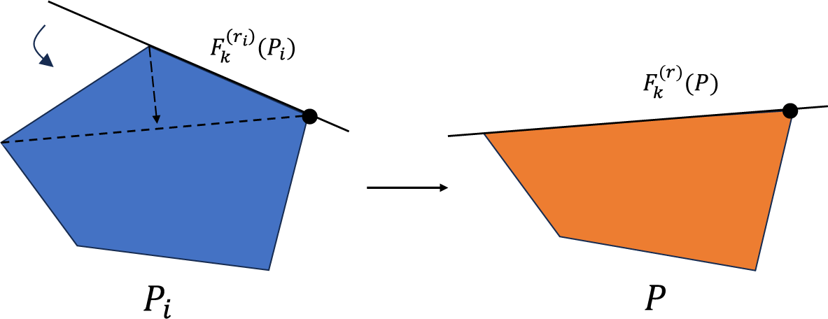
Figure 1 A sequence of polytopes which has facets converging essentially.
Next we consider the $2$
-dimensional case
$2$
-dimensional case $\mathcal {D}_2$
.
$\mathcal {D}_2$
.
Theorem 5.1.5. For a sequence $\{P_i\}_i\subset \mathcal {D}_2$
suppose that
$\{P_i\}_i\subset \mathcal {D}_2$
suppose that $d^H(P_i, P)\to 0 \ (i\to \infty )$
for some
$d^H(P_i, P)\to 0 \ (i\to \infty )$
for some $P\in \mathcal {D}_2$
. If
$P\in \mathcal {D}_2$
. If $\displaystyle \sup_i N_1(P_i)<\infty $
, then for each facet
$\displaystyle \sup_i N_1(P_i)<\infty $
, then for each facet $F^{(r)}_{1}(P)$
of P and its primitive normal vector
$F^{(r)}_{1}(P)$
of P and its primitive normal vector $\nu ^{(r)}$
, there exists
$\nu ^{(r)}$
, there exists $r_i\in \{1,\cdots , N_1(P_i)\}$
such that a subsequence of primitive normal vectors
$r_i\in \{1,\cdots , N_1(P_i)\}$
such that a subsequence of primitive normal vectors $\{\nu _i^{(r_i)}\}_i$
of
$\{\nu _i^{(r_i)}\}_i$
of $F^{(r_i)}_{1}(P_i)$
such that
$F^{(r_i)}_{1}(P_i)$
such that $\nu _i^{(r_i)}\to \nu ^{(r)} \ (i\to \infty )$
.
$\nu _i^{(r_i)}\to \nu ^{(r)} \ (i\to \infty )$
.
Proof. We may assume that $r=1$
. By Corollary 5.1.3 and the semi-continuity of the Hausdorff measure in the non-collapsing limit we may assume that for each facet (=edge)
$r=1$
. By Corollary 5.1.3 and the semi-continuity of the Hausdorff measure in the non-collapsing limit we may assume that for each facet (=edge) $F^{(r)}_{1}(P)$
there exists a sequence
$F^{(r)}_{1}(P)$
there exists a sequence $\{F^{(r_i)}_1(P_i)\}_i$
of facets of
$\{F^{(r_i)}_1(P_i)\}_i$
of facets of $\{P_i\}_i$
which converges essentially to
$\{P_i\}_i$
which converges essentially to $F^{(r)}_1(P)$
. We rearrange the indices so that
$F^{(r)}_1(P)$
. We rearrange the indices so that $r_i=1$
for all i and may assume that the facets are numbered in a counterclockwise way.
$r_i=1$
for all i and may assume that the facets are numbered in a counterclockwise way.
Since $\{F^{(1)}_1(P_i)\}_i$
converges essentially to
$\{F^{(1)}_1(P_i)\}_i$
converges essentially to $F^{(1)}_1(P)$
the sequence of inward unit normal vectors converges:
$F^{(1)}_1(P)$
the sequence of inward unit normal vectors converges:
 $$\begin{align*}\frac{\nu^{(1)}_i}{\|\nu^{(1)}_i\|}\to \frac{\nu^{(1)}}{\|\nu^{(1)}\|} \quad (i\to \infty). \end{align*}$$
Since $\{\nu ^{(1)}_i\}_i$
is a sequence of integral vectors if
$\{\nu ^{(1)}_i\}_i$
is a sequence of integral vectors if $\{\|\nu ^{(1)}_i\|\}_i$
is a bounded sequence, then
$\{\|\nu ^{(1)}_i\|\}_i$
is a bounded sequence, then $\nu ^{(1)}_i=\nu ^{(1)}$
for sufficiently large i, and hence, we have the required subsequence.
$\nu ^{(1)}_i=\nu ^{(1)}$
for sufficiently large i, and hence, we have the required subsequence.
We consider the case that $\{\nu ^{(1)}_i\}_i$
is unbounded. By taking a subsequence we have
$\{\nu ^{(1)}_i\}_i$
is unbounded. By taking a subsequence we have
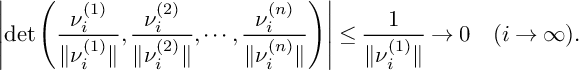
 $$ \begin{align} \left|\det\left(\frac{\nu^{(1)}_i}{\|\nu^{(1)}_i\|}, \frac{\nu^{(2)}_i}{\|\nu^{(2)}_i\|}\right)\right|=\frac{1}{\|\nu_i^{(1)}\|\|\nu_i^{(2)}\|}|\det(\nu_i^{(1)}, \nu_i^{(2)})|\leq \frac{1}{\|\nu_i^{(1)}\|}\to 0 \quad (i\to \infty), \end{align} $$
and hence, we have
 $$ \begin{align} \frac{\nu^{(2)}_i}{\|\nu^{(2)}_i\|}\to \pm\frac{\nu^{(1)}}{\|\nu^{(1)}\|} \quad (i\to \infty). \end{align} $$
We first show the following claim.
Claim. There exists a subsequence of $\{F^{(2)}_1(P_i)\}_i$
which converges to a point or a segment in
$\{F^{(2)}_1(P_i)\}_i$
which converges to a point or a segment in $F_1^{(1)}(P)$
.
$F_1^{(1)}(P)$
.
Proof of the claim
Let $\displaystyle A=\lim _{i\to \infty }F_1^{(1)}(P_i)$
. If
$\displaystyle A=\lim _{i\to \infty }F_1^{(1)}(P_i)$
. If $\displaystyle \lim _{i\to \infty }\mathrm {diam}(F_1^{(2)}(P_i))=0$
, then
$\displaystyle \lim _{i\to \infty }\mathrm {diam}(F_1^{(2)}(P_i))=0$
, then $F_1^{(2)}(P_i)$
converges to a point. In this case
$F_1^{(2)}(P_i)$
converges to a point. In this case $F_1^{(1)}(P_i)\cup F_1^{(2)}(P_i)$
converges to A, and hence
$F_1^{(1)}(P_i)\cup F_1^{(2)}(P_i)$
converges to A, and hence $F_1^{(2)}(P_i)$
converges to a point in A. If
$F_1^{(2)}(P_i)$
converges to a point in A. If $\displaystyle \limsup _{i\to \infty }\mathrm {diam}(F_1^{(2)}(P_i))>0$
, then a subsequence of
$\displaystyle \limsup _{i\to \infty }\mathrm {diam}(F_1^{(2)}(P_i))>0$
, then a subsequence of $F_1^{(2)}(P_i)$
converges to an interval B with positive length. Suppose that
$F_1^{(2)}(P_i)$
converges to an interval B with positive length. Suppose that $\frac {\nu ^{(2)}_i}{\|\nu ^{(2)}_i\|}$
converges to
$\frac {\nu ^{(2)}_i}{\|\nu ^{(2)}_i\|}$
converges to $-\frac {\nu ^{(1)}}{\|\nu ^{(1)}\|}$
. If so then (5.1) implies that for any
$-\frac {\nu ^{(1)}}{\|\nu ^{(1)}\|}$
. If so then (5.1) implies that for any $\varepsilon>0$
the interior angle between
$\varepsilon>0$
the interior angle between $F_1^{(1)}(P_i)$
and
$F_1^{(1)}(P_i)$
and $F_1^{(2)}(P_i)$
is smaller than
$F_1^{(2)}(P_i)$
is smaller than $\varepsilon $
for any
$\varepsilon $
for any $i \gg 0$
. Then we have
$i \gg 0$
. Then we have $|P_i|<(\mathrm {diam}(P_i))\varepsilon $
, which contradicts to
$|P_i|<(\mathrm {diam}(P_i))\varepsilon $
, which contradicts to $P_i \to P$
in
$P_i \to P$
in $d_H$
-topology, and hence, we have
$d_H$
-topology, and hence, we have $\frac {\nu ^{(2)}_i}{\|\nu ^{(2)}_i\|} \to \frac {\nu ^{(1)}}{\|\nu ^{(1)}\|}$
. In particular the interior angle between
$\frac {\nu ^{(2)}_i}{\|\nu ^{(2)}_i\|} \to \frac {\nu ^{(1)}}{\|\nu ^{(1)}\|}$
. In particular the interior angle between $F_1^{(1)}(P_i)$
and
$F_1^{(1)}(P_i)$
and $F_1^{(2)}(P_i)$
converges to
$F_1^{(2)}(P_i)$
converges to $\pi $
, and hence, B is contained in the line which contains A. It implies the claim,
$\pi $
, and hence, B is contained in the line which contains A. It implies the claim, $A\cup B \subset F_1^{(1)}(P)$
.
$A\cup B \subset F_1^{(1)}(P)$
.
By taking a subsequence we may assume that $N_1(P_i)$
is constant for
$N_1(P_i)$
is constant for $i \gg 1$
, say
$i \gg 1$
, say $\sup_i N_1(P_i)$
. We can take the smallest number s so that
$\sup_i N_1(P_i)$
. We can take the smallest number s so that $2\leq s \leq \sup_iN_1(P_i)$
and
$2\leq s \leq \sup_iN_1(P_i)$
and $\{\nu _i^{(s)}\}_i$
is bounded. In fact, if not, then by repeating the argument in the proof of the above claim inductively we see that
$\{\nu _i^{(s)}\}_i$
is bounded. In fact, if not, then by repeating the argument in the proof of the above claim inductively we see that $P_i$
converges to a subset of
$P_i$
converges to a subset of $F_1^{(1)}(P)$
, which is a contradiction. By using the minimality of s and the argument (5.1) repeatedly we have
$F_1^{(1)}(P)$
, which is a contradiction. By using the minimality of s and the argument (5.1) repeatedly we have
 $$\begin{align*}\frac{\nu^{(s)}_i}{\|\nu^{(s)}_i\|}\to \pm \frac{\nu^{(1)}}{\|\nu^{(1)}\|} \quad (i\to \infty). \end{align*}$$
Again, by using the argument in the proof of the above claim repeatedly, we see that by taking a subsequence,
 $$\begin{align*}\bigcup_{1\leq t \leq s-1}F_1^{(t)}(P_i) \end{align*}$$
converges to a segment in $F_1^{(1)}(P)$
and
$F_1^{(1)}(P)$
and $\frac {\nu ^{(s)}_i}{\|\nu ^{(s)}_i\|} $
converges to
$\frac {\nu ^{(s)}_i}{\|\nu ^{(s)}_i\|} $
converges to $\frac {\nu ^{(1)}}{\|\nu ^{(1)}\|}$
as
$\frac {\nu ^{(1)}}{\|\nu ^{(1)}\|}$
as $i\to \infty $
. The boundedness of
$i\to \infty $
. The boundedness of $\{\nu _i^{(s)}\}_i$
implies that this is the required subsequence.
$\{\nu _i^{(s)}\}_i$
implies that this is the required subsequence.
Remark 5.1.6. In Theorem 5.1.5 the boundedness of each sequence of primitive normal vectors $\{\nu _i^{(r_i)}\}_i$
implies that it contains a constant subsequence. In other words, only the constant terms vary in the defining equations of the (sub)sequence
$\{\nu _i^{(r_i)}\}_i$
implies that it contains a constant subsequence. In other words, only the constant terms vary in the defining equations of the (sub)sequence $\{P_i\}_i$
. See Figure 2.
$\{P_i\}_i$
. See Figure 2.
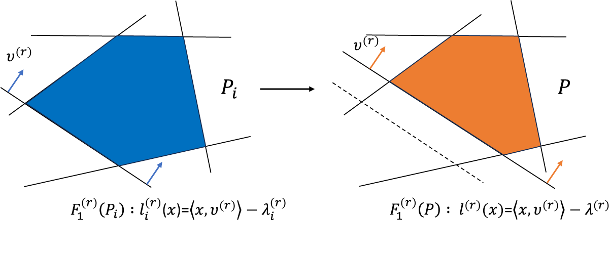
Figure 2 A sequence of polytopes with constant normal vectors.
By the same argument we have the following convergence in the higher dimensional non-degenerate case.
Theorem 5.1.7. For a sequence $\{P_i\}_i\subset \mathcal {D}_n$
suppose that
$\{P_i\}_i\subset \mathcal {D}_n$
suppose that $d^H(P_i, P)\to 0 \ (i\to \infty )$
for some
$d^H(P_i, P)\to 0 \ (i\to \infty )$
for some $P\in \mathcal {D}_n$
and
$P\in \mathcal {D}_n$
and $\displaystyle N_{n-1}(P)=\lim _{i\to \infty } N_{n-1}(P_i)$
. For each facet
$\displaystyle N_{n-1}(P)=\lim _{i\to \infty } N_{n-1}(P_i)$
. For each facet $F^{(r)}(P)$
of P and its primitive normal vector
$F^{(r)}(P)$
of P and its primitive normal vector $\nu ^{(r)}$
, there exists a sequence of primitive normal vectors
$\nu ^{(r)}$
, there exists a sequence of primitive normal vectors $\{\nu _i^{(r_i)}\}_i$
of
$\{\nu _i^{(r_i)}\}_i$
of $F^{(r_i)}(P_i)$
such that
$F^{(r_i)}(P_i)$
such that $\nu _i^{(r_i)}\to \nu ^{(r)} \ (i\to \infty )$
.
$\nu _i^{(r_i)}\to \nu ^{(r)} \ (i\to \infty )$
.
Proof. As in the proof of Theorem 5.1.5 we can take a sequence of primitive normal vectors $\{\nu ^{(1)}_i\}_i$
of
$\{\nu ^{(1)}_i\}_i$
of $\{F^{(1)}(P_i)\}_i$
, and it suffices to show that
$\{F^{(1)}(P_i)\}_i$
, and it suffices to show that $\{\|\nu ^{(1)}_i\|\}_i$
is bounded. Suppose that
$\{\|\nu ^{(1)}_i\|\}_i$
is bounded. Suppose that $\{\|\nu ^{(1)}_i\|\}_i$
is unbounded. Consider a vertex of
$\{\|\nu ^{(1)}_i\|\}_i$
is unbounded. Consider a vertex of $F^{(1)}_{n-1}(P_i)$
and facets around it. We may assume that they are numbered as
$F^{(1)}_{n-1}(P_i)$
and facets around it. We may assume that they are numbered as $r=2,3,\cdots , n$
. Then for their primitive normal vectors we have
$r=2,3,\cdots , n$
. Then for their primitive normal vectors we have
 $$\begin{align*}\left|\det\left(\frac{\nu^{(1)}_i}{\|\nu^{(1)}_i\|}, \frac{\nu^{(2)}_i}{\|\nu^{(2)}_i\|}, \cdots , \frac{\nu^{(n)}_i}{\|\nu^{(n)}_i\|}\right)\right| \leq \frac{1}{\|\nu_i^{(1)}\|}\to 0 \quad (i\to \infty). \end{align*}$$
It contradicts to our assumption $\displaystyle N_{n-1}(P)=\lim _{i\to \infty } N_{n-1}(P_i)$
.
$\displaystyle N_{n-1}(P)=\lim _{i\to \infty } N_{n-1}(P_i)$
.
5.2 From convergence of polytope to convergence of Guillemin metric
We first give the definition of equivariant (measured) Gromov–Hausdorff convergence as a special case of [Reference Fukaya7, Definition 1-3].
Definition 5.2.1. Let $X=(X,d)$
be a compact metric space and
$X=(X,d)$
be a compact metric space and $\{X_i=(X_i,d_i)\}_i$
be a sequence of compact metric spaces. Suppose that there exists a group G which acts on X and each
$\{X_i=(X_i,d_i)\}_i$
be a sequence of compact metric spaces. Suppose that there exists a group G which acts on X and each $X_i$
in an effective and isometric way. Then
$X_i$
in an effective and isometric way. Then $\{X_i\}_i$
converges to X in the G-equivariant Gromov–Hausdorff topology if there exist sequences of maps
$\{X_i\}_i$
converges to X in the G-equivariant Gromov–Hausdorff topology if there exist sequences of maps $\{f_i:X_i\to X\}_i$
, group automorphisms
$\{f_i:X_i\to X\}_i$
, group automorphisms $\{\rho _i:G\to G\}_i$
and positive numbers
$\{\rho _i:G\to G\}_i$
and positive numbers $\{\epsilon _i\}_i$
such that the following conditions hold.
$\{\epsilon _i\}_i$
such that the following conditions hold.
-
1.
$\epsilon _i \to 0$
as
$i\to \infty $
. -
2.
$|d_{i}(x,y)-d(f_i(x), f_i(y))|<\epsilon _i$
for all
$x,y\in X_i$
. -
3. For any
$p\in X$
there exists
$x\in X_i$
such that
$d(p,f_i(x))<\epsilon _i$
. -
4.
$d(f_i(gx), \rho _i(g)f_i(x))<\epsilon _i$
for all
$x\in X_i$
and
$g\in G$
.


When a map $f_i : X_i \to X$
satisfies 2, 3, and 4, respectively, we say that
$f_i : X_i \to X$
satisfies 2, 3, and 4, respectively, we say that $f_i$
is almost isometric, almost surjective and almost equivariant, respectively. This situation will be denoted by
$f_i$
is almost isometric, almost surjective and almost equivariant, respectively. This situation will be denoted by $X_i\xrightarrow {G\text {-eqGH}}X$
(or
$X_i\xrightarrow {G\text {-eqGH}}X$
(or $X_i \to X$
for simplicity) and
$X_i \to X$
for simplicity) and $f_i$
’s are called approximation maps.
$f_i$
’s are called approximation maps.
Moreover if X (resp. $\{X_i\}_i$
) is equipped with a G-invariant measure m (resp.
$\{X_i\}_i$
) is equipped with a G-invariant measure m (resp. $m_i$
) in such a way that
$m_i$
) in such a way that $(X,m)$
(resp.
$(X,m)$
(resp. $(X_i, m_i)$
) is a metric measure space and the push forward measure
$(X_i, m_i)$
) is a metric measure space and the push forward measure $(f_i)_{*}m_i$
converges to m weakly, then we say
$(f_i)_{*}m_i$
converges to m weakly, then we say $\{(X_i, m_i)\}_i$
converges to
$\{(X_i, m_i)\}_i$
converges to $(X, m)$
in the G-equivariant measured Gromov–Hausdorff topology and we will denote
$(X, m)$
in the G-equivariant measured Gromov–Hausdorff topology and we will denote $X_i\xrightarrow {G\text {-eqmGH}}X$
.
$X_i\xrightarrow {G\text {-eqmGH}}X$
.
When we consider about equivariant (measured) Gromov–Hausdorff convergence for Riemannian manifolds, we always assume that the manifolds are equipped with Riemannian distance and Riemannian measure.
As a corollary of Theorem 5.1.7 we have the following convergence theorem of symplectic toric manifolds. We emphasize that we do not put any assumptions on curvatures in our theorem below.
Theorem 5.2.2. For a sequence $\{P_i\}_i\subset \mathcal {D}_n$
suppose that
$\{P_i\}_i\subset \mathcal {D}_n$
suppose that $d^H(P_i, P)\to 0 \ (i\to \infty )$
for
$d^H(P_i, P)\to 0 \ (i\to \infty )$
for $P\in \mathcal {D}_n$
and
$P\in \mathcal {D}_n$
and $\displaystyle N_{n-1}(P)=\lim _{i\to \infty } N_{n-1}(P_i)$
, where
$\displaystyle N_{n-1}(P)=\lim _{i\to \infty } N_{n-1}(P_i)$
, where $N_{n-1}(\cdot )$
is the number of the facets. Then there exists a subsequence of
$N_{n-1}(\cdot )$
is the number of the facets. Then there exists a subsequence of $\{M_{P_i}\}_i$
which converges to
$\{M_{P_i}\}_i$
which converges to $M_P$
with respect to the corresponding Guillemin metrics in the T-equivariant Gromov–Hausdorff topology.
$M_P$
with respect to the corresponding Guillemin metrics in the T-equivariant Gromov–Hausdorff topology.
Proof. We use the same notations as in Section 4.2 with suffix i. We may assume $N=N_{n-1}(P)=N_{n-1}(P_i)=N_i$
. The proof of Theorem 5.1.7 implies that
$N=N_{n-1}(P)=N_{n-1}(P_i)=N_i$
. The proof of Theorem 5.1.7 implies that ${\mathfrak {h}}_i={\mathfrak {h}}$
and
${\mathfrak {h}}_i={\mathfrak {h}}$
and $H_i=H$
for
$H_i=H$
for $i\gg 0$
. Moreover as a corollary of Theorem 5.1.7 we have
$i\gg 0$
. Moreover as a corollary of Theorem 5.1.7 we have $\lambda _{i}^{(r)}\to \lambda ^{(r)}$
(
$\lambda _{i}^{(r)}\to \lambda ^{(r)}$
( $i\to \infty $
) for the constants of the defining equations of
$i\to \infty $
) for the constants of the defining equations of $P_i$
(after renumbering the facets). As a consequence
$P_i$
(after renumbering the facets). As a consequence $(\iota _i^*\circ \tilde \mu _i)^{-1}(0)$
converges to
$(\iota _i^*\circ \tilde \mu _i)^{-1}(0)$
converges to $(\iota ^*\circ \tilde \mu )^{-1}(0)$
in the equivariant Gromov–Hausdorff topologyFootnote
5
. Then
$(\iota ^*\circ \tilde \mu )^{-1}(0)$
in the equivariant Gromov–Hausdorff topologyFootnote
5
. Then $\{M_{P_i}=(\iota _i^*\circ \tilde \mu _i)^{-1}(0)/H_i\}_i$
converges to
$\{M_{P_i}=(\iota _i^*\circ \tilde \mu _i)^{-1}(0)/H_i\}_i$
converges to $M_P=(\iota ^*\circ \tilde \mu )^{-1}(0)/H$
in the Gromov–Hausdorff topology by [Reference Fukaya7, Theorem 2-1]. Moreover the identifications
$M_P=(\iota ^*\circ \tilde \mu )^{-1}(0)/H$
in the Gromov–Hausdorff topology by [Reference Fukaya7, Theorem 2-1]. Moreover the identifications $H_i=H$
induce identifications
$H_i=H$
induce identifications $T_i^n=T^N/H_i=T^N/H=T^n$
, which makes the above convergence into the T-equivariant Gromov–Hausdorff topology.
$T_i^n=T^N/H_i=T^N/H=T^n$
, which makes the above convergence into the T-equivariant Gromov–Hausdorff topology.
Corollary 5.2.3. Under the same assumptions in Theorem 5.2.2, take a subsequence in $\{M_{P_i}\}_i$
which converges to
$\{M_{P_i}\}_i$
which converges to $M_P$
. Then
$M_P$
. Then $M_{P_i}$
are T-equivariantly diffeomorphic to
$M_{P_i}$
are T-equivariantly diffeomorphic to $M_P$
for
$M_P$
for $i\gg 0$
.
$i\gg 0$
.
Proof. By Theorem 5.1.7 we may assume that $\nu _i^{(r)}=\nu ^{(r)}$
for
$\nu _i^{(r)}=\nu ^{(r)}$
for $i\gg 0$
. On the other hand each
$i\gg 0$
. On the other hand each $M_{P_i}$
is T-equivariantly diffeomorphic to the toric variety associated with the fan
$M_{P_i}$
is T-equivariantly diffeomorphic to the toric variety associated with the fan $\Sigma _{P_i}$
. Note that
$\Sigma _{P_i}$
. Note that $\Sigma _{P_i}$
is determined by the normal vectors
$\Sigma _{P_i}$
is determined by the normal vectors $\{\nu _i^{(r)}\}_r$
and it does not depend on
$\{\nu _i^{(r)}\}_r$
and it does not depend on $\{\lambda _i^{(r)}\}_r$
(See [Reference Buchstaber and Panov3] for example). It implies the claim.
$\{\lambda _i^{(r)}\}_r$
(See [Reference Buchstaber and Panov3] for example). It implies the claim.
Remark 5.2.4. The following example shows that it cannot be expected that a convergence of Guillemin metrics to a Guillemin metric as in Theorem 5.2.2 occurs without the assumption $\displaystyle N_{n-1}(P)=\lim _{i\to \infty } N_{n-1}(P_i)$
.
$\displaystyle N_{n-1}(P)=\lim _{i\to \infty } N_{n-1}(P_i)$
.
Consider a sequence of Delzant pentagon $\{P_i\}_i$
defined by 5 inequalities,
$\{P_i\}_i$
defined by 5 inequalities,
 $$\begin{align*}\xi_1\geq 0, \ 1-\xi_1\geq 0, \ \xi_2\geq 0, \ 1-\xi_2\geq 0, \ -\xi_1-\xi_2+(2-1/i)\geq 0, \end{align*}$$
which converges to a rectangle P as in Figure 3.
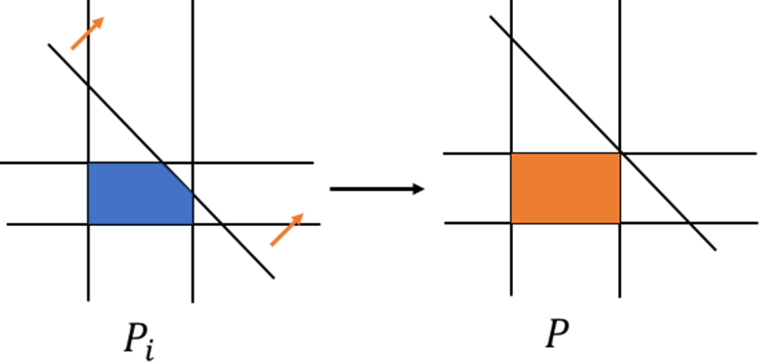
Figure 3 A sequence of pentagons which converges to a rectangle.
It is known that the symplectic toric manifolds $M_{P_i}$
corresponding to each pentagon
$M_{P_i}$
corresponding to each pentagon $P_i$
are (diffeomorphic to) a 1 point blow-up of
$P_i$
are (diffeomorphic to) a 1 point blow-up of $\mathbb {C} P^1\times \mathbb {C} P^1$
. On the other hand the symplectic toric manifold
$\mathbb {C} P^1\times \mathbb {C} P^1$
. On the other hand the symplectic toric manifold $M_P$
corresponding to P is isometric to
$M_P$
corresponding to P is isometric to $\mathbb {C} P^1\times \mathbb {C} P^1$
equipped with the Guillemin metric which is the product metric on
$\mathbb {C} P^1\times \mathbb {C} P^1$
equipped with the Guillemin metric which is the product metric on $\mathbb {C} P^1$
.
$\mathbb {C} P^1$
.
The limiting process $i\to \infty $
gives a smooth convex function
$i\to \infty $
gives a smooth convex function
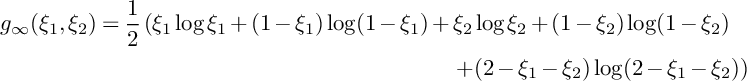 $$ \begin{align*} g_{\infty}(\xi_1,\xi_2)&=\frac{1}{2}\left(\xi_1\log \xi_1 +(1-\xi_1)\log(1-\xi_1)+\xi_2\log \xi_2+(1-\xi_2)\log (1-\xi_2) \right. \\ & \left. \hspace{6cm}+(2-\xi_1-\xi_2)\log(2-\xi_1-\xi_2)\right) \end{align*} $$
on $P^\circ $
. This
$P^\circ $
. This $g_{\infty }$
does not give the Guillemin metric on
$g_{\infty }$
does not give the Guillemin metric on $M_P$
. To deal with these subtle phenomena we have to consider finer structures on
$M_P$
. To deal with these subtle phenomena we have to consider finer structures on $\mathcal {D}_n$
or
$\mathcal {D}_n$
or $\widetilde {\mathcal {D}}_n$
and incorporate potential functions. We will discuss such formulation in a subsequent paper.
$\widetilde {\mathcal {D}}_n$
and incorporate potential functions. We will discuss such formulation in a subsequent paper.
5.3 From convergence of Guillemin metrics to convergence of polytopes
Now let us discuss the convergence of the opposite direction.
Hereafter for each $P\in \mathcal {D}_n$
we denote the symplectic toric manifold equipped with the Guillemin metric by
$P\in \mathcal {D}_n$
we denote the symplectic toric manifold equipped with the Guillemin metric by $M_P=(M_P, \omega _P)$
, and we use the Liouville volume form
$M_P=(M_P, \omega _P)$
, and we use the Liouville volume form $\mathrm {vol}_{M_P}:=\frac {(\omega _P)^{\wedge n}}{n!}$
on the symplectic toric manifold
$\mathrm {vol}_{M_P}:=\frac {(\omega _P)^{\wedge n}}{n!}$
on the symplectic toric manifold $M_P$
. In this way we think
$M_P$
. In this way we think $M_P$
as a metric measure space.
$M_P$
as a metric measure space.
Theorem 5.3.1. Let $\{P_i\}_i$
be a sequence in
$\{P_i\}_i$
be a sequence in $\mathcal {D}_n$
. Suppose that a sequence of symplectic toric manifolds
$\mathcal {D}_n$
. Suppose that a sequence of symplectic toric manifolds $\{M_{P_i}\}_i$
converges to
$\{M_{P_i}\}_i$
converges to $M_P$
for some
$M_P$
for some $P\in \mathcal {D}_n$
with respect to their Guillemin metrics in the T-equivariant measured Gromov–Hausdorff topology. Let
$P\in \mathcal {D}_n$
with respect to their Guillemin metrics in the T-equivariant measured Gromov–Hausdorff topology. Let $\{f_i:M_{P_i}\to M_P\}_i$
be a sequence of approximation maps of the convergence. If
$\{f_i:M_{P_i}\to M_P\}_i$
be a sequence of approximation maps of the convergence. If $\{P_i\}_i$
are contained in a sufficiently large ball in
$\{P_i\}_i$
are contained in a sufficiently large ball in $\mathbb {R}^n$
, then we have
$\mathbb {R}^n$
, then we have
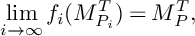 $$\begin{align*}\lim_{i\to\infty}f_i(M_{P_i}^T)=M_P^T, \end{align*}$$
where $M_{P_i}^T$
and
$M_{P_i}^T$
and $M_P^T$
are the fixed point sets of T-actions. In particular we have
$M_P^T$
are the fixed point sets of T-actions. In particular we have
 $$\begin{align*}\liminf_{i\to\infty}\chi(M_{P_i})\geq \chi(M_P), \end{align*}$$
where $\chi (\cdot )$
denotes the Euler characteristic.
$\chi (\cdot )$
denotes the Euler characteristic.
Proof. For simplicity we denote $M_i:=M_{P_i}$
and
$M_i:=M_{P_i}$
and $M:=M_P$
.
$M:=M_P$
.
Fix an arbitrary $\delta>0$
. We show that for any sequence
$\delta>0$
. We show that for any sequence $\{x_i\in M_i^T\}_i$
there exists
$\{x_i\in M_i^T\}_i$
there exists $I\in {\mathbb {N}}$
such that
$I\in {\mathbb {N}}$
such that $f_i(x_i)\in B(M^T, {\delta })$
for any
$f_i(x_i)\in B(M^T, {\delta })$
for any $i>I$
. Suppose that there exists
$i>I$
. Suppose that there exists $\delta>0$
such that
$\delta>0$
such that $f_i(x_i)\notin B(M^T, {\delta })$
for infinitely many i. For
$f_i(x_i)\notin B(M^T, {\delta })$
for infinitely many i. For $\epsilon> 0$
, we define
$\epsilon> 0$
, we define $\delta _\epsilon $
as the minimal
$\delta _\epsilon $
as the minimal $\delta '> 0$
such that if
$\delta '> 0$
such that if $y \not \in B(M^T, \delta ')$
, then
$y \not \in B(M^T, \delta ')$
, then $\operatorname {\mathrm {Diam}}(T\cdot y) \ge \epsilon $
. Note that since M is compact such
$\operatorname {\mathrm {Diam}}(T\cdot y) \ge \epsilon $
. Note that since M is compact such $\delta _\epsilon>0$
exists and
$\delta _\epsilon>0$
exists and $\delta _\epsilon \to 0$
as
$\delta _\epsilon \to 0$
as $\epsilon \to 0$
. Since
$\epsilon \to 0$
. Since $f_i$
is almost T-equivariant we have
$f_i$
is almost T-equivariant we have
 $$\begin{align*}\epsilon_i>d(\rho_i(t)f_i(x_i), f_i(tx_i))=d(\rho_i(t)f_i(x_i), f_i(x_i)) \end{align*}$$
for all $t\in T$
, where
$t\in T$
, where $\{\epsilon _i\}_i$
is a sequence of positive numbers as in Definition 5.2.1 and d is the Riemannian distance of M. It implies that
$\{\epsilon _i\}_i$
is a sequence of positive numbers as in Definition 5.2.1 and d is the Riemannian distance of M. It implies that ${\operatorname {\mathrm {Diam}}}(T\cdot f_i(x_i))<2\epsilon _i\to 0$
as
${\operatorname {\mathrm {Diam}}}(T\cdot f_i(x_i))<2\epsilon _i\to 0$
as $i\to \infty $
. If we take i large enough so that
$i\to \infty $
. If we take i large enough so that $\delta _{\epsilon _i}<\delta $
, then we have
$\delta _{\epsilon _i}<\delta $
, then we have $f_i(x_i)\in B(M^T, {\delta _{\epsilon _i}})$
. It contradicts to
$f_i(x_i)\in B(M^T, {\delta _{\epsilon _i}})$
. It contradicts to $f_i(x_i)\notin B(M^T, {\delta })$
.
$f_i(x_i)\notin B(M^T, {\delta })$
.
Next we show that for any $\delta>0$
there exists
$\delta>0$
there exists $i_0\in \mathbb {N}$
such that
$i_0\in \mathbb {N}$
such that
 $$\begin{align*}f_i^{-1}(M^T)\subset B(M_i^T, {\delta}) \end{align*}$$
holds for all $i>i_0$
. If not then there exists
$i>i_0$
. If not then there exists $\delta>0$
such that we can take
$\delta>0$
such that we can take $x_i\in f_i^{-1}(M^T)$
and
$x_i\in f_i^{-1}(M^T)$
and $x_i\notin B(M_i^T, {\delta })$
for infinitely many i. Since
$x_i\notin B(M_i^T, {\delta })$
for infinitely many i. Since $f_i$
is almost isometry and almost T-equivariant we have
$f_i$
is almost isometry and almost T-equivariant we have
 $$ \begin{align*} d_i(tx_i, x_i)&<d(f_i(tx_i), f_i(x_i))+\epsilon_i \\ &<d(f_i(tx_i), tf_i(x_i))+\epsilon_i \\ &<2\epsilon_i \end{align*} $$
for all $t\in T$
, where
$t\in T$
, where $d_i$
is the Riemannian distance of
$d_i$
is the Riemannian distance of $M_i$
. It implies
$M_i$
. It implies ${\operatorname {\mathrm {Diam}}}(T\cdot x_i)<4\epsilon _i$
. On the other hand it is known that each
${\operatorname {\mathrm {Diam}}}(T\cdot x_i)<4\epsilon _i$
. On the other hand it is known that each $T\cdot x_i$
is a flat torus, and hence,
$T\cdot x_i$
is a flat torus, and hence, ${\operatorname {\mathrm {Diam}}}(T\cdot x_i)\to 0$ $(i\to \infty )$
implies
$(i\to \infty )$
implies $\mathrm {Vol}(T\cdot x_i)\to 0 \ (i\to \infty )$
, where
$\mathrm {Vol}(T\cdot x_i)\to 0 \ (i\to \infty )$
, where $\mathrm {Vol}$
is the Riemannian volume with respect to the induced Riemannian metric. Now consider a compact subset
$\mathrm {Vol}$
is the Riemannian volume with respect to the induced Riemannian metric. Now consider a compact subset $P_i^{\prime }:=\mu _i(M_i\setminus B(M_i^T, \delta ))$
of
$P_i^{\prime }:=\mu _i(M_i\setminus B(M_i^T, \delta ))$
of $P_i$
. Since
$P_i$
. Since $\{M_i\}_i$
converges to M in the measured Gromov–Hausdorff topology
$\{M_i\}_i$
converges to M in the measured Gromov–Hausdorff topology $\{\mathrm {Vol}(M_i)\}_i$
converges to
$\{\mathrm {Vol}(M_i)\}_i$
converges to $\mathrm {Vol}(M)$
. Duistermaat–Heckman’s theorem implies that the Euclidean volumes of
$\mathrm {Vol}(M)$
. Duistermaat–Heckman’s theorem implies that the Euclidean volumes of $\{P_i\}_i$
converge to that of P. In particular they are bounded below by a positive constant. Moreover since we assume that
$\{P_i\}_i$
converge to that of P. In particular they are bounded below by a positive constant. Moreover since we assume that $\{P_i\}_i$
are contained in a ball, the sequence of convex polytopes
$\{P_i\}_i$
are contained in a ball, the sequence of convex polytopes $\{P_i\}_i$
converges to some convex body Q in the Hausdorff distance. As in the same way
$\{P_i\}_i$
converges to some convex body Q in the Hausdorff distance. As in the same way $\{P_i^{\prime }\}_i$
converges to some compact subset
$\{P_i^{\prime }\}_i$
converges to some compact subset $Q'$
of Q. Let
$Q'$
of Q. Let $Q^{(0)}$
be the limit point set of
$Q^{(0)}$
be the limit point set of $\mu _i(M_i^T)=P_i^{(0)}$
. Then we have
$\mu _i(M_i^T)=P_i^{(0)}$
. Then we have $Q^{(0)}\cap Q'=\emptyset $
. When we take
$Q^{(0)}\cap Q'=\emptyset $
. When we take $\delta '>0$
small enough so that
$\delta '>0$
small enough so that $\mathrm {dist}(Q^{(0)},Q' )>2\delta '$
we have
$\mathrm {dist}(Q^{(0)},Q' )>2\delta '$
we have $\mathrm {dist}(P^{(0)}_i, P^{\prime }_i)>\delta '$
. The formula of volumes of the orbits in [Reference Iriyeh and Ono11] impliesFootnote
6
that
$\mathrm {dist}(P^{(0)}_i, P^{\prime }_i)>\delta '$
. The formula of volumes of the orbits in [Reference Iriyeh and Ono11] impliesFootnote
6
that
 $$\begin{align*}\liminf_{i\to \infty}\mathrm{Vol}(T\cdot x_i)>0. \end{align*}$$
It contradicts to $\displaystyle \lim _{i\to \infty }\mathrm {Vol}(T\cdot x_i)=0$
.
$\displaystyle \lim _{i\to \infty }\mathrm {Vol}(T\cdot x_i)=0$
.
The inequality
 $$\begin{align*}\lim_{i\to\infty}\chi(M_{P_i})\geq \chi(M_P), \end{align*}$$
follows from the fact that the Euler characteristic of symplectic toric manifold is equal to the number of fixed points.
Hereafter we discuss the convergence of polytopes under the assumption in Theorem 5.3.1 without boundedness of $\{P_i\}_i$
.
$\{P_i\}_i$
.
Theorem 5.3.2. Let $\{P_i\}_i$
be a sequence in
$\{P_i\}_i$
be a sequence in $\mathcal {D}_n$
. Suppose that a sequence of symplectic toric manifolds
$\mathcal {D}_n$
. Suppose that a sequence of symplectic toric manifolds $\{M_{P_i}\}_i$
converges to
$\{M_{P_i}\}_i$
converges to $M_P$
for some
$M_P$
for some $P\in \mathcal {D}_n$
with respect to their Guillemin metrics in the T-equivariant measured Gromov–Hausdorff topology. Let
$P\in \mathcal {D}_n$
with respect to their Guillemin metrics in the T-equivariant measured Gromov–Hausdorff topology. Let $\{f_i:M_{P_i}\to M_P\}_i$
be a sequence of approximation maps of the convergence. We take and fix a sectionFootnote
7
$\{f_i:M_{P_i}\to M_P\}_i$
be a sequence of approximation maps of the convergence. We take and fix a sectionFootnote
7 $S_i:P_i\to M_{P_i}$
of the moment map
$S_i:P_i\to M_{P_i}$
of the moment map $\mu _i:M_{P_i}\to P_i$
for each i. For each i we define
$\mu _i:M_{P_i}\to P_i$
for each i. For each i we define $\hat f_i:P_i\to P$
by the composition
$\hat f_i:P_i\to P$
by the composition $\hat f_i:=\mu \circ f_i \circ S_i$
.
$\hat f_i:=\mu \circ f_i \circ S_i$
.
Under the above set-up there exists a subsequence of $\{\overline {\hat f_i(P_i)}\}_i$
which converges to P in the
$\{\overline {\hat f_i(P_i)}\}_i$
which converges to P in the $d^H$
-topology.
$d^H$
-topology.
To show Theorem 5.3.2 we prepare two lemmas. Consider the same setting as in Theorem 5.3.2. Let $\mu _i:M_{P_i}\to P_i\subset \mathbb {R}^n$
and
$\mu _i:M_{P_i}\to P_i\subset \mathbb {R}^n$
and $\mu :M_P\to P\subset \mathbb {R}^n$
be the moment maps. For any
$\mu :M_P\to P\subset \mathbb {R}^n$
be the moment maps. For any $\varphi \in C_b(\mathbb {R}^n)$
we define
$\varphi \in C_b(\mathbb {R}^n)$
we define $\tilde \varphi \in C(M_P)$
by
$\tilde \varphi \in C(M_P)$
by $\tilde \varphi :=\varphi \circ \mu $
. Let
$\tilde \varphi :=\varphi \circ \mu $
. Let $\{f_i\}_i$
be a family of approximation maps for
$\{f_i\}_i$
be a family of approximation maps for $M_{P_i}\xrightarrow {T\text {-eqmGH}}M_P$
. We define a sequence of measurable functions
$M_{P_i}\xrightarrow {T\text {-eqmGH}}M_P$
. We define a sequence of measurable functions $\{\tilde \varphi _i:M_{P_i}\to \mathbb {R}\}_i$
by
$\{\tilde \varphi _i:M_{P_i}\to \mathbb {R}\}_i$
by $\tilde \varphi _i:=\tilde \varphi \circ f_i$
. Let
$\tilde \varphi _i:=\tilde \varphi \circ f_i$
. Let $\{(\mathrm {vol}_{M_{P_i}})_y\}_{y\in P_i}$
(resp.
$\{(\mathrm {vol}_{M_{P_i}})_y\}_{y\in P_i}$
(resp. $\{(\mathrm {vol}_{M_{P}})_y\}_{y\in P}$
) be a disintegration (See Appendix B) for
$\{(\mathrm {vol}_{M_{P}})_y\}_{y\in P}$
) be a disintegration (See Appendix B) for $\mu _i:M_{P_i}\to P_i$
(resp.
$\mu _i:M_{P_i}\to P_i$
(resp. $\mu :M_P\to P$
) and define a sequence of measurable functions
$\mu :M_P\to P$
) and define a sequence of measurable functions $\{\varphi _i:P_i\to \mathbb {R}\}_i$
by
$\{\varphi _i:P_i\to \mathbb {R}\}_i$
by
 $$ \begin{align} \varphi_i(y):=\int_{M_{P_i}}\tilde\varphi_i(x)(\mathrm{vol}_{M_{P_i}})_y(dx). \end{align} $$
Lemma 5.3.3. For any $\varphi \in C_b(\mathbb {R}^n)$
the sequence of measurable maps
$\varphi \in C_b(\mathbb {R}^n)$
the sequence of measurable maps $\{\varphi _i: P_i\to \mathbb {R}\}_i$
satisfies
$\{\varphi _i: P_i\to \mathbb {R}\}_i$
satisfies
 $$\begin{align*}\lim_{i\to \infty}\int_{P_i}\varphi_i~d\mathcal{L}^n=\int_{P}\varphi ~d\mathcal{L}^n. \end{align*}$$
Proof. Note that by Duistermaat–Heckman’s theorem we have $(\mu _i)_*(\mathrm {vol}_{M_{P_i}})=\mathcal {L}^n|_{P_i}$
. Since
$(\mu _i)_*(\mathrm {vol}_{M_{P_i}})=\mathcal {L}^n|_{P_i}$
. Since $(f_i)_*(\mathrm {vol}_{M_{P_i}})$
converges to
$(f_i)_*(\mathrm {vol}_{M_{P_i}})$
converges to $\mathrm {vol}_{M_P}$
the claim follows as follows.
$\mathrm {vol}_{M_P}$
the claim follows as follows.
 $$ \begin{align*} \int_{P_i}\varphi_i(y) \mathcal{L}^n(dy)&=\int_{P_i}\left(\int_{M_{P_i}}\tilde\varphi_i(x)(\mathrm{vol}_{M_{P_i}})_y(dx)\right)\mathcal{L}^n(dy)\\ &=\int_{M_{P_i}}\tilde\varphi_i(x)\mathrm{vol}_{M_{P_i}}(dx) \\ &=\int_{M_{P_i}}\tilde\varphi(f_i(x))\mathrm{vol}_{M_{P_i}}(dx) \\ &\xrightarrow[i\to\infty]{} \int_{M_P}\tilde\varphi(x)\mathrm{vol}_{M_P}(dx)\\ &=\int_{P}\left(\int_{M_P}\tilde\varphi(x)(\mathrm{vol}_{M_{P}})_y(dx)\right)\mathcal{L}^n(dy) \\ &=\int_{P}\left(\int_{\mu^{-1}(y)}\varphi(\mu(x))(\mathrm{vol}_{M_{P}})_y(dx)\right)\mathcal{L}^n(dy)\\ &= \int_{P}\left(\int_{\mu^{-1}(y)}\varphi(y)(\mathrm{vol}_{M_{P}})_y(dx)\right)\mathcal{L}^n(dy) \\ &=\int_P\varphi(y)\mathcal{L}^n(dy). \end{align*} $$
Lemma 5.3.4. As in the same setting in Theorem 5.3.2 we have
 $$\begin{align*}\lim_{i\to \infty}\frac{1}{|P_i|}\int_{P_i}\varphi_i d\mathcal{L}^n=\lim_{i\to\infty}\frac{1}{|P_i|}\int_{P_i}\varphi\circ \hat f_i d\mathcal{L}^n. \end{align*}$$
for any $\varphi \in C_b(\mathbb {R}^n)$
, where
$\varphi \in C_b(\mathbb {R}^n)$
, where $\varphi _i$
are as in (5.3).
$\varphi _i$
are as in (5.3).
Proof. Let $\{\rho _i:T^n\to T^n\}_i$
be a sequence of automorphisms as in Definition 5.2.1 for
$\{\rho _i:T^n\to T^n\}_i$
be a sequence of automorphisms as in Definition 5.2.1 for $M_{P_i}\xrightarrow {\mathrm {eq-m}GH}M_P$
. Fix
$M_{P_i}\xrightarrow {\mathrm {eq-m}GH}M_P$
. Fix $\eta>0$
and
$\eta>0$
and $\varphi \in C_b(\mathbb {R}^n)$
. For any
$\varphi \in C_b(\mathbb {R}^n)$
. For any $y\in P_i$
we have
$y\in P_i$
we have
 $$ \begin{align} |\varphi_i(y)-\varphi(F_i(y))| \leq \int_{\mu_i^{-1}(y)}|\varphi(\mu(f_i(x)))-\varphi(\mu(f_i(S_i(y))))|(\mathrm{vol}_{M_{P_i}})_y(dx). \end{align} $$
Since for any $x\in \mu _i^{-1}(y)$
there exists
$x\in \mu _i^{-1}(y)$
there exists $t_x\in T$
such that
$t_x\in T$
such that $x=t_x\cdot S_i(y)$
we have
$x=t_x\cdot S_i(y)$
we have
 $$ \begin{align*} \|\mu(f_i(x))-\mu(f_i(S_i(y)))\|&=\|\mu(f_i(t_x\cdot S_i(y)))-\mu(f_i(S_i(y)))\| \\ &= \|\mu(f_i(t_x\cdot S_i(y)))-\mu(\rho_i(t_x)\cdot f_i(S_i(y)))\|. \end{align*} $$
On the other hand since $\varphi $
and
$\varphi $
and $\mu $
are uniformly continuous and
$\mu $
are uniformly continuous and $\{M_{P_i}\}_i$
converges to
$\{M_{P_i}\}_i$
converges to $M_P$
in the T-equivariant Gromov–Hausdorff topology there exists
$M_P$
in the T-equivariant Gromov–Hausdorff topology there exists $i_0\in \mathbb {N}$
such that if
$i_0\in \mathbb {N}$
such that if $i>i_0$
, then
$i>i_0$
, then
 $$\begin{align*}|\varphi(\mu(f_i(x)))-\varphi(\mu(f_i(S_i(y))))|=|\varphi(\mu(f_i(x)))-\varphi(\mu(\rho_i(t_x)\cdot f_i(S_i(y))))|<\eta. \end{align*}$$
In particular we have
 $$\begin{align*}|\varphi_i(y)-\varphi(\hat f_i(y))|<\eta \end{align*}$$
in (5.4), and hence,
 $$\begin{align*}\frac{1}{|P_i|}\left|\int_{P_i}(\varphi_i(y)-\varphi(\hat f_i(y)))\mathcal{L}^n(dy)\right|<\eta. \end{align*}$$
Note that our assumption $M_{P_i}\xrightarrow {T\text {-eqmGH}}M_P$
and Duistermaat–Heckman’s theorem imply
$M_{P_i}\xrightarrow {T\text {-eqmGH}}M_P$
and Duistermaat–Heckman’s theorem imply $|P_i|=\mathrm {vol}_{M_{P_i}}(M_{P_i})\to |P|=\mathrm {vol}_{M_{P}}(M_{P})$
. Since
$|P_i|=\mathrm {vol}_{M_{P_i}}(M_{P_i})\to |P|=\mathrm {vol}_{M_{P}}(M_{P})$
. Since $\eta>0$
is arbitrary the limit of
$\eta>0$
is arbitrary the limit of $\displaystyle \frac {1}{|P_i|}\int _{P_i}\varphi _i(y)\mathcal {L}^n(dy)$
exists and we have the required equality
$\displaystyle \frac {1}{|P_i|}\int _{P_i}\varphi _i(y)\mathcal {L}^n(dy)$
exists and we have the required equality
 $$\begin{align*}\lim_{i\to\infty}\frac{1}{|P_i|}\int_{P_i}\varphi_i(y)\mathcal{L}^n(dy)= \lim_{i\to\infty}\frac{1}{|P_i|}\int_{P_i}\varphi(\hat f_i(y))\mathcal{L}^n(dy). \end{align*}$$
Proof of Theorem 5.3.2
Let $\varphi \in C_b(\mathbb {R}^n)$
. By Lemmas 5.3.3 and 5.3.4, we have a sequence of measurable maps
$\varphi \in C_b(\mathbb {R}^n)$
. By Lemmas 5.3.3 and 5.3.4, we have a sequence of measurable maps $\{\hat f_i:P_i\to P\}_i$
and measurable functions
$\{\hat f_i:P_i\to P\}_i$
and measurable functions $\{\varphi _i:P_i\to \mathbb {R}\}_i$
such that
$\{\varphi _i:P_i\to \mathbb {R}\}_i$
such that
 $$\begin{align*}\lim_{i\to\infty}\int_P\varphi(y)(\hat f_i)_*(\mathcal{L}^n)(dy)= \lim_{i\to\infty}\int_{P_i}\varphi_i(y)\mathcal{L}^n(dy) =\int_P\varphi(y)\mathcal{L}^n(dy). \end{align*}$$
Note that we have $|P_i|\to |P| \ (i\to \infty )$
under our assumption, measured Gromov–Hausdorff convergence, and Duistermaat–Heckman’s theorem. This equality implies that the sequence of probability measures
$|P_i|\to |P| \ (i\to \infty )$
under our assumption, measured Gromov–Hausdorff convergence, and Duistermaat–Heckman’s theorem. This equality implies that the sequence of probability measures $\{(\hat f_i)_{*}m_{P_i}\}_i$
converges weakly to
$\{(\hat f_i)_{*}m_{P_i}\}_i$
converges weakly to $m_{P}$
.
$m_{P}$
.
Now we show that
 $$ \begin{align} \inf_i\inf_{x\in P}(\hat f_i)_*(m_i)(B_{\epsilon}(x))>0 \end{align} $$
for all $\epsilon>0$
. If not, then there exists
$\epsilon>0$
. If not, then there exists $\epsilon _0>0$
, a sequence of natural numbers
$\epsilon _0>0$
, a sequence of natural numbers $\{i_j\}_j$
and a sequence of points
$\{i_j\}_j$
and a sequence of points $\{x_{j}\}_j$
in P such that
$\{x_{j}\}_j$
in P such that
 $$\begin{align*}(\hat f_{i_j})_*(m_{i_j})(B_{\epsilon_0}(x_j))\to 0 \quad (j\to \infty). \end{align*}$$
Since P is compact there is an accumulation point $x_\infty $
of
$x_\infty $
of $\{x_{j}\}_j$
and we have
$\{x_{j}\}_j$
and we have
 $$\begin{align*}B_{\epsilon_0/2}(x_\infty)\subset B_{\epsilon_0}(x_j) \end{align*}$$
for infinitely many j. Then we have a contradiction
 $$ \begin{align*} 0<m_P(B_{\epsilon/2}(x_\infty)) &\leq \liminf_j (\hat f_{i_j})_*(m_{i_j})(B_{\epsilon_0/2}(x_\infty)) \\ &\leq \liminf_j(\hat f_{i_j})_*(m_{i_j})(B_{\epsilon_0}(x_j))=0. \end{align*} $$
The weak convergence of $\{(\hat f_i)_{*}m_{P_i}\}_i$
to
$\{(\hat f_i)_{*}m_{P_i}\}_i$
to $m_{P}$
implies the
$m_{P}$
implies the $\square $
-convergence of a sequence of metric measure spaces
$\square $
-convergence of a sequence of metric measure spaces $\{(P, (\hat f_i)_{*}m_{P_i})\}$
to
$\{(P, (\hat f_i)_{*}m_{P_i})\}$
to $(P,m_P)$
by [Reference Shioya16, Proposition 4.12]. Moreover the
$(P,m_P)$
by [Reference Shioya16, Proposition 4.12]. Moreover the $\square $
-convergence and (5.5) imply the measured Gromov–Hausdorff convergence of
$\square $
-convergence and (5.5) imply the measured Gromov–Hausdorff convergence of $\{(P, (\hat f_i)_{*}m_{P_i})\}$
to
$\{(P, (\hat f_i)_{*}m_{P_i})\}$
to $(P,m_P)$
by [Reference Shioya16, Remark 4.34], which in particular implies the Hausdorff convergence of
$(P,m_P)$
by [Reference Shioya16, Remark 4.34], which in particular implies the Hausdorff convergence of $\{\mathrm {supp}\,((\hat f_i)_{*}m_{P_i})=\overline {\hat f_i(P_i)}\}_i$
to
$\{\mathrm {supp}\,((\hat f_i)_{*}m_{P_i})=\overline {\hat f_i(P_i)}\}_i$
to $\mathrm {supp}\,(m_P)=P$
.
$\mathrm {supp}\,(m_P)=P$
.
Remark 5.3.5. Regarding Theorem 5.3.2 it is natural to consider the convergence of $\{P_i\}_i$
itself to P in the Gromov–Hausdorff or
$\{P_i\}_i$
itself to P in the Gromov–Hausdorff or $d^H$
-topology. One can see that this is not true in the literal sense because of the ambiguity of the affine transformation groups
$d^H$
-topology. One can see that this is not true in the literal sense because of the ambiguity of the affine transformation groups $G_n$
. We could address these problems in terms of the moduli space. Namely one may hope that if
$G_n$
. We could address these problems in terms of the moduli space. Namely one may hope that if $\{M_{P_i}\}_i$
converges to
$\{M_{P_i}\}_i$
converges to $M_P$
in the T-equivariant measured Gromov–Hausdorff topology, then there exists a sequence
$M_P$
in the T-equivariant measured Gromov–Hausdorff topology, then there exists a sequence $\{\varphi _i\}_i$
in
$\{\varphi _i\}_i$
in $G_n$
such that
$G_n$
such that $\{\varphi _i(P_i)\}_i$
converges to P in the Gromov–Hausdorff or
$\{\varphi _i(P_i)\}_i$
converges to P in the Gromov–Hausdorff or $d^H$
-topology. It would be useful to consider minimum variance elements explained in Remark 3.2.4.
$d^H$
-topology. It would be useful to consider minimum variance elements explained in Remark 3.2.4.
§A. Preliminaries on probability measures and
$L^2$
-Wasserstein distance.

In this appendix we summarize several facts on probability measures and $L^2$
-Wasserstein distance. For more details consult [Reference Villani18] for example.
$L^2$
-Wasserstein distance. For more details consult [Reference Villani18] for example.
Let $\mathscr {P}(\mathbb {R}^n)$
be the set of all complete Borel probability measures on
$\mathscr {P}(\mathbb {R}^n)$
be the set of all complete Borel probability measures on $\mathbb {R}^n$
. Consider the subset of
$\mathbb {R}^n$
. Consider the subset of $\mathscr {P}(\mathbb {R}^n)$
consisting of measures with finite quadratic moment,
$\mathscr {P}(\mathbb {R}^n)$
consisting of measures with finite quadratic moment,
 $$ \begin{align*} \mathscr{P}_2(\mathbb{R}^n)&:=\left\{m\in\mathscr{P}(\mathbb{R}^n) \ \middle| \ \exists o\in\mathbb{R}^n, \ \int_{\mathbb{R}^n}\|x-o\|^2m(dx)<\infty\right\}. \end{align*} $$
A.1. Weak convergence and Prokhorov’s theorem
Definition A.1.1. A sequence $\{m_i\}_i$
in
$\{m_i\}_i$
in $\mathscr {P}(\mathbb {R}^n)$
converges weakly to
$\mathscr {P}(\mathbb {R}^n)$
converges weakly to $m\in \mathscr {P}(\mathbb {R}^n)$
 $$\begin{align*}\lim_{i\to\infty}\int_{\mathbb{R}^n}f(x)m_i(dx)=\int_{\mathbb{R}^n}f(x)m(dx) \end{align*}$$
for any bounded continuous function f on $\mathbb {R}^n$
.
$\mathbb {R}^n$
.
Theorem A.1.2. For a sequence $\{m_i\}_i$
in
$\{m_i\}_i$
in $\mathscr {P}(\mathbb {R}^n)$
and
$\mathscr {P}(\mathbb {R}^n)$
and $m\in \mathscr {P}(\mathbb {R}^n)$
the followings are equivalent.
$m\in \mathscr {P}(\mathbb {R}^n)$
the followings are equivalent.
-
1.
$\{m_i\}_i$
converges weakly to m. -
2. For any open subset U in
$\mathbb {R}^n$
we have
$\displaystyle \liminf _{i\to \infty } m_i(U)\geq m(U)$
. -
3. For any closed subset C in
$\mathbb {R}^n$
we have
$\displaystyle \limsup _{i\to \infty } m_i(C)\leq m(C)$
. -
4. For any Borel subset A in
$\mathbb {R}^n$
with
$m(\overline {A}\setminus A^{\circ })=0$
we have
$\displaystyle \lim _{i\to \infty } m_i(A)= m(A)$
.


Theorem A.1.3 (Prokhorov’s theorem).
A subset $\mathcal {K}\subset \mathcal {P}(\mathbb {R}^n)$
is relatively compact with respect to the weak convergence topology if and only if for all
$\mathcal {K}\subset \mathcal {P}(\mathbb {R}^n)$
is relatively compact with respect to the weak convergence topology if and only if for all $\epsilon>0$
there exists a compact subset
$\epsilon>0$
there exists a compact subset $K\subset \mathbb {R}^n$
such thatFootnote
8
$K\subset \mathbb {R}^n$
such thatFootnote
8
 $$ \begin{align*} \sup_{ m\in\mathcal{K}} m(\mathbb{R}^n\setminus K)<\epsilon. \end{align*} $$
For a weak convergent sequence of probability measure the following is well-known. See [Reference Ambrosio, Gigli and Savaré2] for example.
Theorem A.1.4. If $\{ m_i\}_i\subset \mathcal {P}(\mathbb {R}^n)$
has a weak convergent limit
$\{ m_i\}_i\subset \mathcal {P}(\mathbb {R}^n)$
has a weak convergent limit $ m \in \mathcal {P}(\mathbb {R}^n)$
, then for any
$ m \in \mathcal {P}(\mathbb {R}^n)$
, then for any $x\in \mathrm {supp}\,(m)$
there exists
$x\in \mathrm {supp}\,(m)$
there exists $x_i\in \mathrm {supp}\,(m_i)$
such that
$x_i\in \mathrm {supp}\,(m_i)$
such that $x_i\rightarrow x$
.
$x_i\rightarrow x$
.
A.2.
$L^2$
-Wasserstein distance of probability measures

For $m, m'\in \mathscr {P}_2(\mathbb {R}^n)$
let
$m, m'\in \mathscr {P}_2(\mathbb {R}^n)$
let $\mathsf {Cpl}(m, m')$
be the set of all couplings between m and
$\mathsf {Cpl}(m, m')$
be the set of all couplings between m and $m'$
. Namely
$m'$
. Namely $\mathsf {Cpl}(m, m')$
is the set of measures
$\mathsf {Cpl}(m, m')$
is the set of measures $\xi \in \mathscr {P}(\mathbb {R}^n\times \mathbb {R}^n)$
such that for any Borel subset A of
$\xi \in \mathscr {P}(\mathbb {R}^n\times \mathbb {R}^n)$
such that for any Borel subset A of $\mathbb {R}^n$
it satisfies
$\mathbb {R}^n$
it satisfies
 $$ \begin{align*} \begin{cases} \xi(A\times \mathbb{R}^n)=m(A)\\ \xi(\mathbb{R}^n\times A)=m'(A). \end{cases} \end{align*} $$
The $L^2$
-Wasserstein distance between
$L^2$
-Wasserstein distance between $m, m'\in \mathscr {P}_2(\mathbb {R}^m)$
is defined by
$m, m'\in \mathscr {P}_2(\mathbb {R}^m)$
is defined by
 $$ \begin{align*} W_2(m,m'):=\inf\left\{ \left(\int_{\mathbb{R}^n\times\mathbb{R}^n}\|x-y\|^2\xi(dx, dy)\right)^{1/2} \ \middle| \ \xi\in\mathsf{Cpl}(m,m')\right\}. \end{align*} $$
It is known that $W_2$
is a metric on
$W_2$
is a metric on $\mathscr {P}_2(\mathbb {R}^n)$
and
$\mathscr {P}_2(\mathbb {R}^n)$
and $(\mathscr {P}_2(\mathbb {R}^n), W_2)$
is a complete separable metric space with the following properties.
$(\mathscr {P}_2(\mathbb {R}^n), W_2)$
is a complete separable metric space with the following properties.
Theorem A.2.1. For a sequence $\{m_i\}_i$
in
$\{m_i\}_i$
in $\mathscr {P}_2(\mathbb {R}^n)$
and
$\mathscr {P}_2(\mathbb {R}^n)$
and $m\in \mathscr {P}_2(\mathbb {R}^n)$
the followings are equivalent.
$m\in \mathscr {P}_2(\mathbb {R}^n)$
the followings are equivalent.
-
1.
$W_2(m_i,m)\rightarrow 0$
(
$i\to \infty $
). -
2.
$\{m_i\}_i$
converges weakly to m and
$$ \begin{align*} \lim_{R\rightarrow\infty}\limsup_{i\rightarrow \infty}\int_{\mathbb{R}^n\setminus B(o,R)}\|x-o\|^2m_i(dx)=0. \end{align*} $$
-
3. For any continuous function
$\varphi $
such that
$\vert \varphi (x)\vert \leq C(1+\|x_0-x\|)^2$
for some
$C>0$
,
$x_0\in \mathbb {R}^n$
the following holds
$$ \begin{align*} \lim_{i\rightarrow\infty}\int_{\mathbb{R}^n}\varphi\,dm_i=\int_{\mathbb{R}^n}\varphi\,dm. \end{align*} $$


Recall that if for $m, m'\in \mathscr {P}_2(\mathbb {R}^n)$
there exists a Borel measurable map
$m, m'\in \mathscr {P}_2(\mathbb {R}^n)$
there exists a Borel measurable map $T:\mathbb {R}^n\to \mathbb {R}^n$
such that
$T:\mathbb {R}^n\to \mathbb {R}^n$
such that $T_{*} m=m'$
and
$T_{*} m=m'$
and $(\mathsf {id}\times T)_*m\in \mathsf {Opt}(m,m')$
, then we say that the Monge problem for
$(\mathsf {id}\times T)_*m\in \mathsf {Opt}(m,m')$
, then we say that the Monge problem for $m, m'$
admits a solution and T is called a solution of the Monge problem.
$m, m'$
admits a solution and T is called a solution of the Monge problem.
Theorem A.2.2. For $m, m'\in \mathscr {P}_2(\mathbb {R}^n)$
if
$m, m'\in \mathscr {P}_2(\mathbb {R}^n)$
if $m\ll \mathcal {L}^n$
, then there is a solution of the Monge problem for m and
$m\ll \mathcal {L}^n$
, then there is a solution of the Monge problem for m and $m'$
. The solution is unique in the following sense. For another solution
$m'$
. The solution is unique in the following sense. For another solution $S:\mathbb {R}^n\to \mathbb {R}^n$
we have
$S:\mathbb {R}^n\to \mathbb {R}^n$
we have $m(\{T\neq S\})=0$
.
$m(\{T\neq S\})=0$
.
Corollary A.2.3. For $m,m'\in \mathscr {P}_2(\mathbb {R}^n)$
with
$m,m'\in \mathscr {P}_2(\mathbb {R}^n)$
with $m\ll \mathcal {L}^n$
and a sequence
$m\ll \mathcal {L}^n$
and a sequence $\{m^{\prime }_i\}_i$
in
$\{m^{\prime }_i\}_i$
in $\mathscr {P}_2(\mathbb {R}^n)$
which converges weakly to
$\mathscr {P}_2(\mathbb {R}^n)$
which converges weakly to $m'$
, there exists a solution
$m'$
, there exists a solution $T:\mathbb {R}^n\to \mathbb {R}^n$
of the Monge problem for m,
$T:\mathbb {R}^n\to \mathbb {R}^n$
of the Monge problem for m, $m'$
and a sequence
$m'$
and a sequence $\{T_i\}_i$
of solutions of the Monge problem for m,
$\{T_i\}_i$
of solutions of the Monge problem for m, $m_i^{\prime }$
with
$m_i^{\prime }$
with
 $$ \begin{align*} m\left(\left\{x\in\mathbb{R}^n \ | \ \vert T_i(x)-T(x)\vert\geq \epsilon\right\}\right)\rightarrow 0 \ (i\to \infty). \end{align*} $$
§B. Disintegration theorem
We use the following type of disintegration theorem. See [Reference Garling8, Theorem 16.10.1] for example.
Theorem B.0.1. Let X and Y be complete separable metric spaces. Let m be a $\sigma $
-finite Borel probability measure and
$\sigma $
-finite Borel probability measure and $f:X\to Y$
a Borel measurable map. Suppose that the push forward
$f:X\to Y$
a Borel measurable map. Suppose that the push forward $f_*m$
is a
$f_*m$
is a $\sigma $
-finite measure on Y. Then there exists a family of probability measures
$\sigma $
-finite measure on Y. Then there exists a family of probability measures $\{m_y\}_{y\in Y}$
on X such that for each Borel subset A the map
$\{m_y\}_{y\in Y}$
on X such that for each Borel subset A the map
 $$\begin{align*}Y\ni y\mapsto m_y(A)\in[0,1] \end{align*}$$
is Borel measurable and for each Borel measurable function $\varphi $
on X we have
$\varphi $
on X we have
 $$\begin{align*}\int_X\varphi~dm =\int_Y\left(\int_X\varphi(x) m_y(dx)\right)f_*m(dy). \end{align*}$$
Moreover we have
 $$\begin{align*}m_y(f^{-1}(y))=1 \quad (y\in Y \ (f_*m\text{-a.e}) ). \end{align*}$$
The above family of measures $\{m_y\}_{y\in Y}$
is called a disintegration for
$\{m_y\}_{y\in Y}$
is called a disintegration for $f:X\to Y$
.
$f:X\to Y$
.
Acknowledgements
This work was partially done while the first author was visiting the Department of Mathematics, University of Toronto, and the Department of Mathematics and Statistics, McMaster University. He would like to thank both institutions for their hospitality, especially for L. Jeffrey and M. Harada. He is also grateful to Y. Karshon and X. Tang for fruitful discussions. The first author is partly supported by Grant-in-Aid for Scientific Research (C) 18K03288 and (C) 24K06719. The second author is partly supported by Grant-in-Aid for Early-Career Scientists 18K13412, Scientific Research (C) 21K03238 and (C) 22K03291. The third author is partly supported by Grant-in-Aid for Young Scientists (B) 15K17529, Scientific Research (A) 17H01091, (C) 20K03598, (B) 21H00977 and (C) 24K06725. Finally, the authors would like to express gratitude to K. Ohashi who gave us a chance to begin this research.


