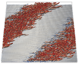
1. Introduction
In fluid mechanics, plane Couette flow (pCf) demonstrates the flow of a viscous fluid between two infinite parallel plates in relative motion. This shear-driven flow has attracted attention from researchers for many decades. It is distinct from other wall-bounded flows in the sense that the total shear stress in pCf is constant across the channel. As in other canonical flows, turbulence brings complexity to pCf. Therefore, specially designed experiments and direct numerical simulations (DNS) are required to study pCf when it is in the turbulent regime. El Telbany & Reynolds (Reference El Telbany and Reynolds1980) conducted experiments to study the velocity distribution in fully turbulent pCf and formulated empirical descriptions for velocities in various sublayers. In a follow-up study (El Telbany & Reynolds Reference El Telbany and Reynolds1981), they also developed an empirical explanation for stresses near the walls and in the channel core. Experiments to study the various aspects of pCf have an inherent challenge of capturing all higher-order statistics due to complications arising from a moving boundary (Aydin & Leutheusser Reference Aydin and Leutheusser1979). DNS do not have such limitations and a study done by Lee & Kim (Reference Lee and Kim1991) explored the flow structures in fully turbulent pCf and compared their results with those of the plane Poiseuille flow. The major difference that they have noticed in pCf is the existence of large-scale high- and low-velocity structures elongated in the streamwise direction, which fill the entire channel in the wall-normal direction. The secondary flow that they reported consists of large counter-rotating vortices or roll cells. Later researchers such as Kristoffersen, Bech & Andersson (Reference Kristoffersen, Bech and Andersson1993) and Bech et al. (Reference Bech, Tillmark, Alfredsson and Andersson1995) also reported roll cells but the mechanism which gave rise to these vortices was not clear. In the investigation by Hamilton, Kim & Waleffe (Reference Hamilton, Kim and Waleffe1995) the mechanism of formation of roll cells and their role in sustaining the elongated streaks was elaborated. They proposed the concept of a regeneration cycle, which comprises three stages: formation of elongated streaks from the streamwise vorticity associated with roll cells, breakdown of streaks to generate three-dimensional vorticity and regeneration of streamwise vorticity. It appears that this cycle sustains the streaks and counter-rotating vortices which are salient to the fully turbulent regime in pCf.
Only a few decades before, research was successful in discovering the flow features that accompany transition in pCf. The earliest transition studies in pCf were reported by Aydin & Leutheusser (Reference Aydin and Leutheusser1991), Tillmark & Alfredsson (Reference Tillmark and Alfredsson1992), Daviaud, Hegseth & Bergé (Reference Daviaud, Hegseth and Bergé1992) and Malerud, Målo/y & Goldburg (Reference Malerud, Målo/y and Goldburg1995). Prigent et al. (Reference Prigent, Grégoire, Chaté and Dauchot2003) were one of the first researchers to study detailed flow features in transitional pCf. They discovered that the transition takes place through a stage of oblique laminar–turbulent bands, which are periodic in the streamwise and spanwise directions. These bands exist within the range of ![]() $Re \in [325,415]$. Thus, the flow is fully turbulent above the upper threshold (
$Re \in [325,415]$. Thus, the flow is fully turbulent above the upper threshold (![]() $Re_{t}\approx 415$) and laminar below the lower threshold (
$Re_{t}\approx 415$) and laminar below the lower threshold (![]() $Re_{g}\approx 325$). Their experiments were performed in a large-aspect ratio set-up owing to the large wavelengths of the bands. Performing a DNS in a large domain is computationally challenging. Barkley & Tuckerman (Reference Barkley and Tuckerman2005) were the first to capture transition bands using DNS. They used a tilted domain in place of a large-aspect-ratio domain and thereby save the computational cost. In another study (Barkley & Tuckerman Reference Barkley and Tuckerman2007), they focused on the mean flow aspect of transitional pCf. One main highlight from the aforementioned study is that the mean streamwise velocity in the laminar zones in the transitional regime is not linear, which is why research community refer to these regions in the pattern as quasi-laminar. Another significant outcome from their study is a model which connects the wall-normal profiles of mean flow and the Reynolds stresses. The appearance of laminar–turbulent bands does not always require a fully resolved DNS simulation. Under-resolved simulations can also capture the transition pattern but with a reduction in the transitional Reynolds number range (Manneville Reference Manneville2011; Manneville & Rolland Reference Manneville and Rolland2011). Apart from the difference in critical Reynolds number, all other aspects of the bands remain the same. As mentioned earlier, alternating laminar–turbulent bands demand the computational domain to be very large. The question of how large a domain is needed is of interest. Philip & Manneville (Reference Philip and Manneville2011) suggested an answer to this question by simulating transitional pCf in domains of different diagonal lengths (
$Re_{g}\approx 325$). Their experiments were performed in a large-aspect ratio set-up owing to the large wavelengths of the bands. Performing a DNS in a large domain is computationally challenging. Barkley & Tuckerman (Reference Barkley and Tuckerman2005) were the first to capture transition bands using DNS. They used a tilted domain in place of a large-aspect-ratio domain and thereby save the computational cost. In another study (Barkley & Tuckerman Reference Barkley and Tuckerman2007), they focused on the mean flow aspect of transitional pCf. One main highlight from the aforementioned study is that the mean streamwise velocity in the laminar zones in the transitional regime is not linear, which is why research community refer to these regions in the pattern as quasi-laminar. Another significant outcome from their study is a model which connects the wall-normal profiles of mean flow and the Reynolds stresses. The appearance of laminar–turbulent bands does not always require a fully resolved DNS simulation. Under-resolved simulations can also capture the transition pattern but with a reduction in the transitional Reynolds number range (Manneville Reference Manneville2011; Manneville & Rolland Reference Manneville and Rolland2011). Apart from the difference in critical Reynolds number, all other aspects of the bands remain the same. As mentioned earlier, alternating laminar–turbulent bands demand the computational domain to be very large. The question of how large a domain is needed is of interest. Philip & Manneville (Reference Philip and Manneville2011) suggested an answer to this question by simulating transitional pCf in domains of different diagonal lengths (![]() $L=\sqrt {L_{x}^{2}+L_{y}^{2}}$, where
$L=\sqrt {L_{x}^{2}+L_{y}^{2}}$, where ![]() $L_{x}$ and
$L_{x}$ and ![]() $L_{y}$ are the domain dimensions in the streamwise and spanwise directions, respectively). They found that the spatiotemporal dynamics associated with pattern formation require a domain with a diagonal length of at least
$L_{y}$ are the domain dimensions in the streamwise and spanwise directions, respectively). They found that the spatiotemporal dynamics associated with pattern formation require a domain with a diagonal length of at least ![]() $87.3h$ as domains of size less than that yield an abrupt transition from the turbulent regime to the laminar regime without an intermediate pattern stage. Duguet, Schlatter & Henningson (Reference Duguet, Schlatter and Henningson2010) performed a DNS in a large-aspect-ratio system to capture the competition between bands with different angles, which is otherwise impossible to capture in short domains. They also found that a pattern angle of
$87.3h$ as domains of size less than that yield an abrupt transition from the turbulent regime to the laminar regime without an intermediate pattern stage. Duguet, Schlatter & Henningson (Reference Duguet, Schlatter and Henningson2010) performed a DNS in a large-aspect-ratio system to capture the competition between bands with different angles, which is otherwise impossible to capture in short domains. They also found that a pattern angle of ![]() $40^\circ$ is more probable to arise during band formation as it requires the least initial energy to carry on. Duguet & Schlatter (Reference Duguet and Schlatter2013) studied how oblique laminar–turbulent bands emerge from turbulent spots. According to them, the large-scale flow is responsible for advecting the streaks inside the turbulent spots in an oblique fashion, giving rise to oblique laminar–turbulent bands.
$40^\circ$ is more probable to arise during band formation as it requires the least initial energy to carry on. Duguet & Schlatter (Reference Duguet and Schlatter2013) studied how oblique laminar–turbulent bands emerge from turbulent spots. According to them, the large-scale flow is responsible for advecting the streaks inside the turbulent spots in an oblique fashion, giving rise to oblique laminar–turbulent bands.
It is difficult to find perfectly smooth surfaces in practical engineering applications. Therefore, there is a need to conduct experiments and simulations of fluid flow under the influence of roughness. One of the earlier works that addressed the effect of roughness was by Nikuradse (Reference Nikuradse1933). Nikuradse used a pipe with an inner wall covered with sand grains of varying roughness and measured the pressure drop and bulk velocity to calculate the friction factor. Roughness increases friction and leads to a higher pressure drop. When it comes to turbulent pCf, only very few studies have considered the effect of roughness. In their pCf experiments, Aydin & Leutheusser (Reference Aydin and Leutheusser1991) used a staggered array of spherical plastic beads as roughness elements on both the walls. They used a towing tank set-up for the purpose. Compared with their smooth case, the hydrodynamically rough case (surprisingly) showed lower values of streamwise velocity fluctuations. One of the first DNS studies in rough turbulent Couette flows was by Javanappa & Narasimhamurthy (Reference Javanappa and Narasimhamurthy2020, Reference Javanappa and Narasimhamurthy2021, Reference Javanappa and Narasimhamurthy2022). They placed square-shaped two-dimensional (2-D) roughness elements on the stationary wall, and the moving wall was smooth. Their study reveals the presence of counter-rotating secondary vortices aligned in the streamwise direction in both the smooth and the rough cases. In the rough case, the streaks are distorted and reduced to fine-scale structures near the roughness elements. Even fewer studies have considered the effect of roughness on the transition to turbulence in pCf. Ishida et al. (Reference Ishida, Brethouwer, Duguet and Tsukahara2017) studied the influence of roughness on transitional pCf. They, however, did not use actual roughness elements, but a roughness model proposed by Busse & Sandham (Reference Busse and Sandham2012) was used. In the case of one rough wall, a new regime involving transverse turbulent bands was found for all roughness heights greater than 30 ![]() $\%$ of half-channel height. Another observation is a downwards shift in the transitional range due to roughness. Tsukahara et al. (Reference Tsukahara, Tomioka, Ishida, Duguet and Brethouwer2018) conducted a follow-up study to confirm the existence of transverse turbulent bands. They quadrupled the domain size and studied its influence. Even though the bandwidth changes, the transverse turbulent bands remain robust to domain change. As opposed to oblique turbulent bands, transverse turbulent bands are wider and do not exhibit significant band parallel flow. Another difference is the presence of very intense streaks at the laminar–turbulent interfaces of transverse turbulent bands.
$\%$ of half-channel height. Another observation is a downwards shift in the transitional range due to roughness. Tsukahara et al. (Reference Tsukahara, Tomioka, Ishida, Duguet and Brethouwer2018) conducted a follow-up study to confirm the existence of transverse turbulent bands. They quadrupled the domain size and studied its influence. Even though the bandwidth changes, the transverse turbulent bands remain robust to domain change. As opposed to oblique turbulent bands, transverse turbulent bands are wider and do not exhibit significant band parallel flow. Another difference is the presence of very intense streaks at the laminar–turbulent interfaces of transverse turbulent bands.
Most experimental and numerical studies dealt with the transition to turbulence in pCf considered smooth walls. Only a few works in the literature study the effect of roughness on transition in pCf, and none of them has used real roughness elements. The present study is, thereby, novel as it intends to study transition in pCf in the presence of real roughness elements. Particular attention is given to studying the various aspects such as spatiotemporal intermittency, large-scale flow, mean secondary flow and Reynolds stresses, in rough pCf. We also investigate the effect of pitch separation of 2-D roughness elements on the transitional range.
2. Methodology
A schematic of rough pCf is shown in figure 1. Two parallel plates are separated by a wall-normal (![]() $z$) distance of
$z$) distance of ![]() $2h$. Here
$2h$. Here ![]() $L_{x}$ and
$L_{x}$ and ![]() $L_{y}$ are the dimensions of the computational domain in the streamwise (
$L_{y}$ are the dimensions of the computational domain in the streamwise (![]() $x$) and spanwise (
$x$) and spanwise (![]() $\kern 1.5pt y$) directions, respectively. The top plate moves at a constant velocity
$\kern 1.5pt y$) directions, respectively. The top plate moves at a constant velocity ![]() $U_{w}$ in the
$U_{w}$ in the ![]() $x$ direction, and the bottom plate is stationary. The stationary wall is mounted with 2-D roughness elements. The important parameters in rough Couette flows are the roughness height (
$x$ direction, and the bottom plate is stationary. The stationary wall is mounted with 2-D roughness elements. The important parameters in rough Couette flows are the roughness height (![]() $k$), the width (
$k$), the width (![]() $w$) and the streamwise pitch separation (
$w$) and the streamwise pitch separation (![]() $\lambda$). We use roughness elements of height
$\lambda$). We use roughness elements of height ![]() $k=0.2h$ with a square cross-section (
$k=0.2h$ with a square cross-section (![]() $k=w$) and vary the pitch separation to study its influence on transition to turbulence. Perry, Schofield & Joubert (Reference Perry, Schofield and Joubert1969) classified surface roughness as d-type and k-type roughness. In the d-type roughness, the elements are closely spaced, forming stable recirculations in the narrow cavities. The outer flow is relatively undisturbed as vortex shedding above the roughness crest is negligible. In the k-type roughness, the cavities are wide; therefore, the ribs are subjected to the outer flow. Eddies of a length scale proportional to
$k=w$) and vary the pitch separation to study its influence on transition to turbulence. Perry, Schofield & Joubert (Reference Perry, Schofield and Joubert1969) classified surface roughness as d-type and k-type roughness. In the d-type roughness, the elements are closely spaced, forming stable recirculations in the narrow cavities. The outer flow is relatively undisturbed as vortex shedding above the roughness crest is negligible. In the k-type roughness, the cavities are wide; therefore, the ribs are subjected to the outer flow. Eddies of a length scale proportional to ![]() $k$ are shed above the roughness crest. According to Jiménez (Reference Jiménez2004), the roughness behaviour transitions from d-type to k-type when the cavities become wider than three to four times the roughness height
$k$ are shed above the roughness crest. According to Jiménez (Reference Jiménez2004), the roughness behaviour transitions from d-type to k-type when the cavities become wider than three to four times the roughness height ![]() $k$. The relative importance of frictional drag compared with pressure drag varies with the type of roughness. In the d-type roughness, frictional drag dominates, whereas in the k-type roughness, pressure drag is more significant (Leonardi, Orlandi & Antonia Reference Leonardi, Orlandi and Antonia2007). In the present study, we have the d-type (
$k$. The relative importance of frictional drag compared with pressure drag varies with the type of roughness. In the d-type roughness, frictional drag dominates, whereas in the k-type roughness, pressure drag is more significant (Leonardi, Orlandi & Antonia Reference Leonardi, Orlandi and Antonia2007). In the present study, we have the d-type (![]() $\lambda = 2k$) and the k-type (
$\lambda = 2k$) and the k-type (![]() $\lambda = 10k$) rough cases. Transition to turbulence in the smooth pCf is also simulated for comparison with the rough pCf.
$\lambda = 10k$) rough cases. Transition to turbulence in the smooth pCf is also simulated for comparison with the rough pCf.
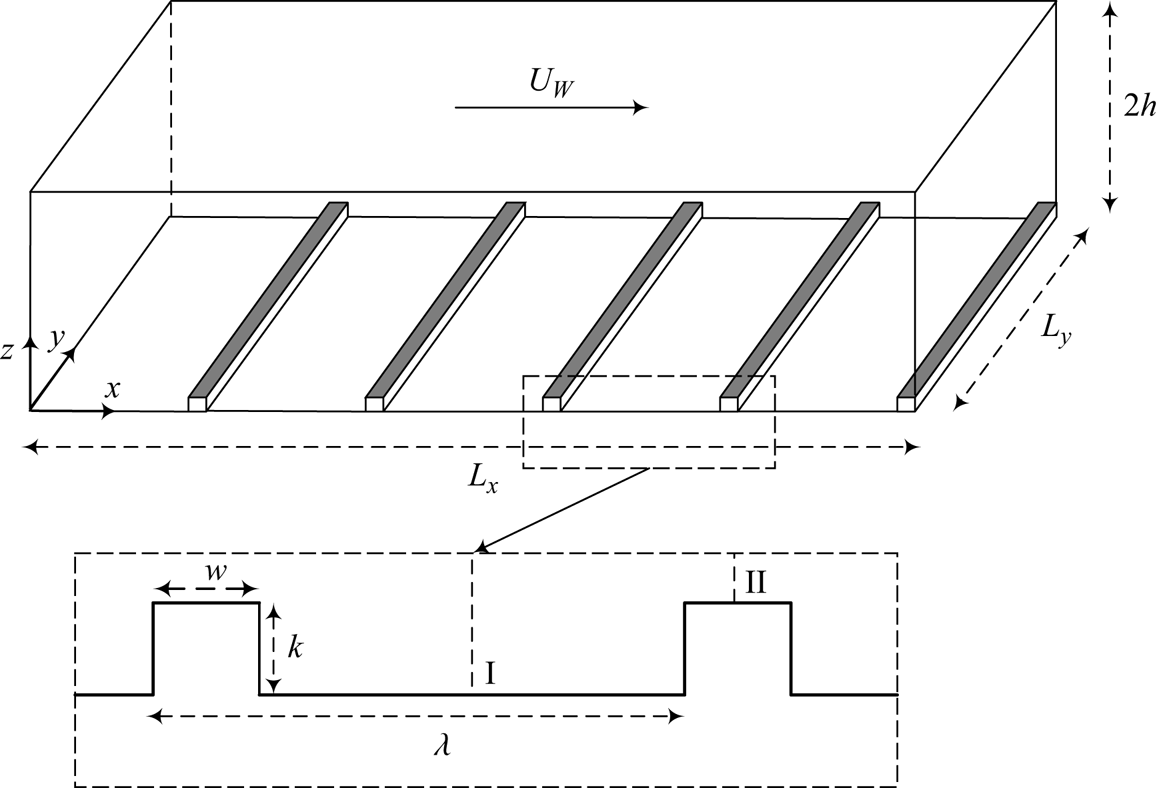
Figure 1. Schematic of rough Couette flow with roughness elements on the stationary wall. Within a pitch, I and II indicate the midcavity and midrib locations, respectively.
The fluid that occupies the gap between the parallel plates is Newtonian, and the flow is considered incompressible. The three-dimensional incompressible Navier Stokes equations that govern the fluid flow are solved using the in-house finite-volume code, MGLET (Manhart Reference Manhart2004):
where ![]() $u$ is the velocity, the subscripts
$u$ is the velocity, the subscripts ![]() $i$ and
$i$ and ![]() $j$ are indices and
$j$ are indices and ![]() $p$ is the pressure. The Reynolds number
$p$ is the pressure. The Reynolds number ![]() $(Re=U_{w}h/2\nu )$ is defined based on the half-channel height (
$(Re=U_{w}h/2\nu )$ is defined based on the half-channel height (![]() $h$) and half the velocity difference between the plates (
$h$) and half the velocity difference between the plates (![]() $U_{w}/2$). The code uses a staggered Cartesian grid arrangement, where the pressure is stored at the cell centres, and velocities are stored at the cell faces. It employs a central difference scheme for spatial discretisation. Adams–Bashforth scheme (second-order accurate) is used to perform time integration. A multi-grid method is used to accelerate the Poisson equation solution to get the pressure. Streamwise and spanwise directions of the domain have periodic boundary conditions, and a no-slip boundary condition is imposed on the plates and the rib surfaces.
$U_{w}/2$). The code uses a staggered Cartesian grid arrangement, where the pressure is stored at the cell centres, and velocities are stored at the cell faces. It employs a central difference scheme for spatial discretisation. Adams–Bashforth scheme (second-order accurate) is used to perform time integration. A multi-grid method is used to accelerate the Poisson equation solution to get the pressure. Streamwise and spanwise directions of the domain have periodic boundary conditions, and a no-slip boundary condition is imposed on the plates and the rib surfaces.
A computational domain of size ![]() $L_{x} \times L_{y} \times L_{z} = 136h \times 68h \times 2h$ is used in the present study. It is large enough to accommodate a single wavelength of the laminar–turbulent bands and is of the same size as Ishida et al. (Reference Ishida, Brethouwer, Duguet and Tsukahara2017) (see table 1). The number of cells in the
$L_{x} \times L_{y} \times L_{z} = 136h \times 68h \times 2h$ is used in the present study. It is large enough to accommodate a single wavelength of the laminar–turbulent bands and is of the same size as Ishida et al. (Reference Ishida, Brethouwer, Duguet and Tsukahara2017) (see table 1). The number of cells in the ![]() $x$,
$x$, ![]() $y$ and
$y$ and ![]() $z$ directions (
$z$ directions (![]() $N_{x}$,
$N_{x}$, ![]() $N_{y}$ and
$N_{y}$ and ![]() $N_{z}$) is 4080, 288 and 108, respectively, and is finer than that used in Ishida et al. (Reference Ishida, Brethouwer, Duguet and Tsukahara2017) and Tsukahara et al. (Reference Tsukahara, Tomioka, Ishida, Duguet and Brethouwer2018). The grid in the
$N_{z}$) is 4080, 288 and 108, respectively, and is finer than that used in Ishida et al. (Reference Ishida, Brethouwer, Duguet and Tsukahara2017) and Tsukahara et al. (Reference Tsukahara, Tomioka, Ishida, Duguet and Brethouwer2018). The grid in the ![]() $x$ and
$x$ and ![]() $y$ directions is uniform, whereas the grid in the
$y$ directions is uniform, whereas the grid in the ![]() $z$ direction is non-uniform, with a minimum at the plates and the rib surfaces and a maximum at the channel centre. The meshing is done in such a way that all the vertical faces of the ribs coincide with the cell faces. To get an accurate assessment of the flow near a rib, we have 6 cells along a rib in the
$z$ direction is non-uniform, with a minimum at the plates and the rib surfaces and a maximum at the channel centre. The meshing is done in such a way that all the vertical faces of the ribs coincide with the cell faces. To get an accurate assessment of the flow near a rib, we have 6 cells along a rib in the ![]() $x$ direction and 20 cells within a rib in the
$x$ direction and 20 cells within a rib in the ![]() $z$ direction. The grid resolutions for the rough cases are given in table 2. We have used the same domain for the smooth case, but the mesh size is different. The grid resolutions in the
$z$ direction. The grid resolutions for the rough cases are given in table 2. We have used the same domain for the smooth case, but the mesh size is different. The grid resolutions in the ![]() $x$ and
$x$ and ![]() $z$ directions are reduced as the ribs are not present in the smooth pCf (see table 2). The Grötzbach criterion states that the grid size
$z$ directions are reduced as the ribs are not present in the smooth pCf (see table 2). The Grötzbach criterion states that the grid size ![]() $\Delta = (\Delta x \Delta y \Delta z)^{1/3}$ should be less than
$\Delta = (\Delta x \Delta y \Delta z)^{1/3}$ should be less than ![]() ${\rm \pi} \eta$, where
${\rm \pi} \eta$, where ![]() $\eta$ is the Kolmogorov length scale (Grötzbach Reference Grötzbach1983). The Kolmogorov length scale is defined in theory as
$\eta$ is the Kolmogorov length scale (Grötzbach Reference Grötzbach1983). The Kolmogorov length scale is defined in theory as ![]() $\eta = ({\nu ^{3}}/{\epsilon })^{{1}/{4}}$, where
$\eta = ({\nu ^{3}}/{\epsilon })^{{1}/{4}}$, where ![]() $\nu$ is the kinematic viscosity of the fluid, and
$\nu$ is the kinematic viscosity of the fluid, and ![]() $\epsilon$ is the dissipation rate of turbulent kinetic energy, which is calculated using the expression
$\epsilon$ is the dissipation rate of turbulent kinetic energy, which is calculated using the expression ![]() $\epsilon = \nu \overline {({\partial u_{i}^{\prime }}/{\partial x_{j}})({\partial u_{i}^{\prime }}/{\partial x_{j}})}$. The grids used in all the cases in the present study satisfy the Grötzbach criterion (see figure 2).
$\epsilon = \nu \overline {({\partial u_{i}^{\prime }}/{\partial x_{j}})({\partial u_{i}^{\prime }}/{\partial x_{j}})}$. The grids used in all the cases in the present study satisfy the Grötzbach criterion (see figure 2).
Table 1. Details of the major DNS studies in transitional pCf. Here ![]() $k$ and
$k$ and ![]() $\lambda$ are the roughness height and pitch, respectively,
$\lambda$ are the roughness height and pitch, respectively, ![]() $L_{x}$,
$L_{x}$, ![]() $L_{y}$ and
$L_{y}$ and ![]() $L_{z}$ refer to the domain dimensions in
$L_{z}$ refer to the domain dimensions in ![]() $x$,
$x$, ![]() $y$ and
$y$ and ![]() $z$, respectively and
$z$, respectively and ![]() $N_{x}$,
$N_{x}$, ![]() $N_{y}$ and
$N_{y}$ and ![]() $N_{z}$ is the corresponding number of cells or grid points or spectral modes.
$N_{z}$ is the corresponding number of cells or grid points or spectral modes.
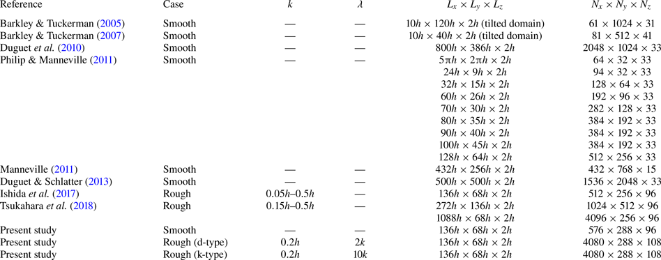
Table 2. Details of the simulations carried out in the present study. The grid resolutions (![]() $\Delta x^{+}$,
$\Delta x^{+}$, ![]() $\Delta y^{+}$ and
$\Delta y^{+}$ and ![]() $\Delta z^{+}$) are based on the global friction Reynolds number
$\Delta z^{+}$) are based on the global friction Reynolds number ![]() $Re_{\tau }$ of each case.
$Re_{\tau }$ of each case.

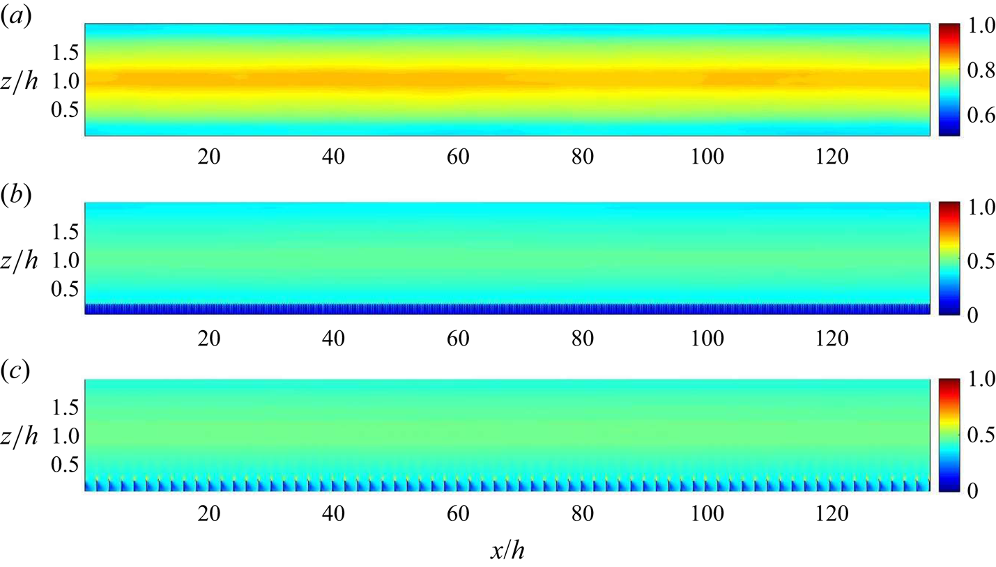
Figure 2. Contours of ![]() $\varDelta / {\rm \pi}\eta$ at
$\varDelta / {\rm \pi}\eta$ at ![]() $Re=500$ shown in an
$Re=500$ shown in an ![]() $x$–
$x$–![]() $z$ plane at
$z$ plane at ![]() $y=34h$ for (a) smooth pCf, (b) d-type roughness and (c) k-type roughness.
$y=34h$ for (a) smooth pCf, (b) d-type roughness and (c) k-type roughness.
An adiabatic protocol (Ishida et al. Reference Ishida, Brethouwer, Duguet and Tsukahara2017; Gokul & Narasimhamurthy Reference Gokul and Narasimhamurthy2022) is a computational procedure, where the Reynolds number is gradually reduced in steps. The term adiabatic protocol comes from the adiabatic process in quantum mechanics, where it is used as synonym for a gradual process. It should not be mistaken for the adiabatic process in thermodynamics, as it has a different meaning. This computational technique is used in the present study to achieve the reverse transition. Starting from a turbulent state at ![]() $Re=500$, the Reynolds number is reduced in steps of 25 until the flow becomes laminar. Statistical stationarity has been achieved at every intermediate Reynolds number. The time step taken in the simulations (
$Re=500$, the Reynolds number is reduced in steps of 25 until the flow becomes laminar. Statistical stationarity has been achieved at every intermediate Reynolds number. The time step taken in the simulations (![]() $\Delta t = 0.01$) is much smaller than the Kolmogorov time scale (Kolmogorov Reference Kolmogorov1941) and satisfies the Courant–Friedrichs–Lewy (CFL) stability criterion. After achieving stationarity at a particular Reynolds number, the simulation is run further to collect samples for getting the averaged quantities. The mean values are obtained by averaging over
$\Delta t = 0.01$) is much smaller than the Kolmogorov time scale (Kolmogorov Reference Kolmogorov1941) and satisfies the Courant–Friedrichs–Lewy (CFL) stability criterion. After achieving stationarity at a particular Reynolds number, the simulation is run further to collect samples for getting the averaged quantities. The mean values are obtained by averaging over ![]() $2500$ samples separated by
$2500$ samples separated by ![]() $0.2h/U_{w}$. The wall-normal variation of mean quantities for the rough pCf cases will be presented at the midcavity (I) and midrib (II) locations, obtained by averaging across time (
$0.2h/U_{w}$. The wall-normal variation of mean quantities for the rough pCf cases will be presented at the midcavity (I) and midrib (II) locations, obtained by averaging across time (![]() $T$),
$T$), ![]() $y$ direction and the pitches (
$y$ direction and the pitches (![]() $N$) in the
$N$) in the ![]() $x$ direction:
$x$ direction:
 \begin{equation} \bar{f}=\frac{1}{N}\frac{1}{L_{y}}\frac{1}{T} \sum_{1}^{N}\int_{0}^{L_{y}}\int_{0}^{T}f\, {\rm d} t\, {\rm d} y.\\ \end{equation}
The averaging across the pitches in the ![]() $x$ direction is due to the periodic nature of the mean flow (Ashrafian, Andersson & Manhart Reference Ashrafian, Andersson and Manhart2004; Nagano, Hattori & Houra Reference Nagano, Hattori and Houra2004; Javanappa & Narasimhamurthy Reference Javanappa and Narasimhamurthy2021). However, the mean quantities in the smooth pCf are averaged across time (
$x$ direction is due to the periodic nature of the mean flow (Ashrafian, Andersson & Manhart Reference Ashrafian, Andersson and Manhart2004; Nagano, Hattori & Houra Reference Nagano, Hattori and Houra2004; Javanappa & Narasimhamurthy Reference Javanappa and Narasimhamurthy2021). However, the mean quantities in the smooth pCf are averaged across time (![]() $T$),
$T$), ![]() $y$ and
$y$ and ![]() $x$ directions:
$x$ directions:
Before embarking on the current problem, a smooth pCf case at ![]() $Re=1300$ is simulated to validate the code. The computational domain used for the validation case is of size
$Re=1300$ is simulated to validate the code. The computational domain used for the validation case is of size ![]() $L_{x} \times L_{y} \times L_{z} = 50.24h \times 16.8h \times 2h$. The corresponding grid used is
$L_{x} \times L_{y} \times L_{z} = 50.24h \times 16.8h \times 2h$. The corresponding grid used is ![]() $N_{x} \times N_{y} \times N_{z} = 640 \times 320 \times 192$. The grid resolutions are uniform in
$N_{x} \times N_{y} \times N_{z} = 640 \times 320 \times 192$. The grid resolutions are uniform in ![]() $x$ and
$x$ and ![]() $y$ directions (
$y$ directions (![]() $\Delta x^{+} = 6.64$ and
$\Delta x^{+} = 6.64$ and ![]() $\Delta y^{+} = 4.44$), whereas the grid resolution in
$\Delta y^{+} = 4.44$), whereas the grid resolution in ![]() $z$ direction is non-uniform and varies from
$z$ direction is non-uniform and varies from ![]() $\Delta z^{+} = 0.2$ at the walls to
$\Delta z^{+} = 0.2$ at the walls to ![]() $\Delta z^{+} = 2.3$ at the channel centre. The results are plotted along with those from Bech et al. (Reference Bech, Tillmark, Alfredsson and Andersson1995), Holstad, Andersson & Pettersen (Reference Holstad, Andersson and Pettersen2010) and Hu, Morfey & Sandham (Reference Hu, Morfey and Sandham2003) (see figure 3). The validation results are in good agreement.
$\Delta z^{+} = 2.3$ at the channel centre. The results are plotted along with those from Bech et al. (Reference Bech, Tillmark, Alfredsson and Andersson1995), Holstad, Andersson & Pettersen (Reference Holstad, Andersson and Pettersen2010) and Hu, Morfey & Sandham (Reference Hu, Morfey and Sandham2003) (see figure 3). The validation results are in good agreement.
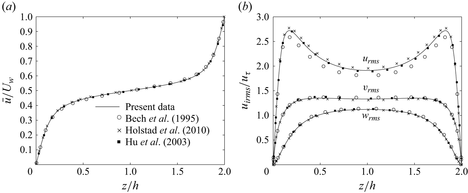
Figure 3. Variation of (a) mean streamwise velocity normalised by ![]() $U_{w}$ and (b) root-mean-square velocities normalised by friction velocity
$U_{w}$ and (b) root-mean-square velocities normalised by friction velocity ![]() $u_{\tau }$ at
$u_{\tau }$ at ![]() $Re=1300$.
$Re=1300$.
3. Results and discussion
We first simulate the base flow at ![]() $Re=500$ before starting the adiabatic procedure. The flow is allowed to come to a stationary state before the samples are collected to calculate the averaged quantities. The turbulent flow statistics at
$Re=500$ before starting the adiabatic procedure. The flow is allowed to come to a stationary state before the samples are collected to calculate the averaged quantities. The turbulent flow statistics at ![]() $Re=500$ for the rough pCf cases are presented in Appendix A for the reader's reference. The Reynolds number is gradually reduced in steps of 25 from
$Re=500$ for the rough pCf cases are presented in Appendix A for the reader's reference. The Reynolds number is gradually reduced in steps of 25 from ![]() $Re=500$ until the flow reaches a laminar state. The results presented at every intermediate Reynolds number are obtained after achieving a statistical stationary state at the intermediate stage. The contours of streamwise velocity
$Re=500$ until the flow reaches a laminar state. The results presented at every intermediate Reynolds number are obtained after achieving a statistical stationary state at the intermediate stage. The contours of streamwise velocity ![]() $u$ in the midgap (
$u$ in the midgap (![]() $z=h$) for the d-type roughness at various Reynolds numbers are shown in figure 4. The flow is turbulent for
$z=h$) for the d-type roughness at various Reynolds numbers are shown in figure 4. The flow is turbulent for ![]() $Re \geq 475$. The turbulent flow is characterised by spanwise alternating high- and low-velocity streaks stretching out in the streamwise direction. When the Reynolds number is reduced to
$Re \geq 475$. The turbulent flow is characterised by spanwise alternating high- and low-velocity streaks stretching out in the streamwise direction. When the Reynolds number is reduced to ![]() $450$, a few laminar spots appear in the turbulent surroundings. At this point, the laminar–turbulent coexistence has not developed into the laminar–turbulent bands. Kashyap, Duguet & Dauchot (Reference Kashyap, Duguet and Dauchot2022) have provided evidence that the pattern stage emerges from the spatial modulation of featureless turbulence caused by linear instabilities. Without disregarding the effect of such linear interactions, Gomé, Tuckerman & Barkley (Reference Gomé, Tuckerman and Barkley2023b) established a more complex mechanism involving the laminar spots. They found that a reduction in
$450$, a few laminar spots appear in the turbulent surroundings. At this point, the laminar–turbulent coexistence has not developed into the laminar–turbulent bands. Kashyap, Duguet & Dauchot (Reference Kashyap, Duguet and Dauchot2022) have provided evidence that the pattern stage emerges from the spatial modulation of featureless turbulence caused by linear instabilities. Without disregarding the effect of such linear interactions, Gomé, Tuckerman & Barkley (Reference Gomé, Tuckerman and Barkley2023b) established a more complex mechanism involving the laminar spots. They found that a reduction in ![]() $Re$ yields laminar spots that are more probable and long-lasting, which eventually self-organise and form regular laminar–turbulent bands. On reducing the Reynolds number to
$Re$ yields laminar spots that are more probable and long-lasting, which eventually self-organise and form regular laminar–turbulent bands. On reducing the Reynolds number to ![]() $Re=425$, oblique laminar–turbulent bands become visible. There is an initial transient during which pattern fronts of different angles compete, and stable bands eventually emerge in the flow field (Prigent et al. Reference Prigent, Grégoire, Chaté and Dauchot2003). These stable patterns are observed for all Reynolds numbers in the range
$Re=425$, oblique laminar–turbulent bands become visible. There is an initial transient during which pattern fronts of different angles compete, and stable bands eventually emerge in the flow field (Prigent et al. Reference Prigent, Grégoire, Chaté and Dauchot2003). These stable patterns are observed for all Reynolds numbers in the range ![]() $Re \in [350,425]$. In the present study, all observations in the transitional range are made after the emergence of stable laminar–turbulent bands. In the presence of transient turbulence, a shorter observation time can adversely affect the results (Bottin & Chaté Reference Bottin and Chaté1998; Hof et al. Reference Hof, Westerweel, Schneider and Eckhardt2006; Avila et al. Reference Avila, Moxey, De Lozar, Avila, Barkley and Hof2011; Avila, Barkley & Hof Reference Avila, Barkley and Hof2023). Therefore, statistical stationarity has been achieved at all
$Re \in [350,425]$. In the present study, all observations in the transitional range are made after the emergence of stable laminar–turbulent bands. In the presence of transient turbulence, a shorter observation time can adversely affect the results (Bottin & Chaté Reference Bottin and Chaté1998; Hof et al. Reference Hof, Westerweel, Schneider and Eckhardt2006; Avila et al. Reference Avila, Moxey, De Lozar, Avila, Barkley and Hof2011; Avila, Barkley & Hof Reference Avila, Barkley and Hof2023). Therefore, statistical stationarity has been achieved at all ![]() $Re$ considered in this study. The width of the turbulent bands shrink with a reduction in Reynolds number, which indicates flow shifting gradually towards the laminar regime. On reducing the Reynolds number to
$Re$ considered in this study. The width of the turbulent bands shrink with a reduction in Reynolds number, which indicates flow shifting gradually towards the laminar regime. On reducing the Reynolds number to ![]() $Re=325$, the turbulent bands shrink further and finally disappear from the flow field, resulting in a laminar flow. In the k-type roughness, the flow remains turbulent for Reynolds numbers up to
$Re=325$, the turbulent bands shrink further and finally disappear from the flow field, resulting in a laminar flow. In the k-type roughness, the flow remains turbulent for Reynolds numbers up to ![]() $Re=375$ (see figure 5). A further reduction to
$Re=375$ (see figure 5). A further reduction to ![]() $Re=350$ yields a few laminar spots in the turbulent environment. The laminar–turbulent coexistence takes the form of laminar–turbulent bands at
$Re=350$ yields a few laminar spots in the turbulent environment. The laminar–turbulent coexistence takes the form of laminar–turbulent bands at ![]() $Re=325$, and they are sustained in the flow up to
$Re=325$, and they are sustained in the flow up to ![]() $Re=300$. Therefore, the bands are stable for all Reynolds numbers in the range
$Re=300$. Therefore, the bands are stable for all Reynolds numbers in the range ![]() $Re \in [300,325]$. Similar to the d-type roughness, there is a reduction in the width of turbulent bands when the Reynolds number is decreased. The flow finally laminarises at
$Re \in [300,325]$. Similar to the d-type roughness, there is a reduction in the width of turbulent bands when the Reynolds number is decreased. The flow finally laminarises at ![]() $Re=275$.
$Re=275$.
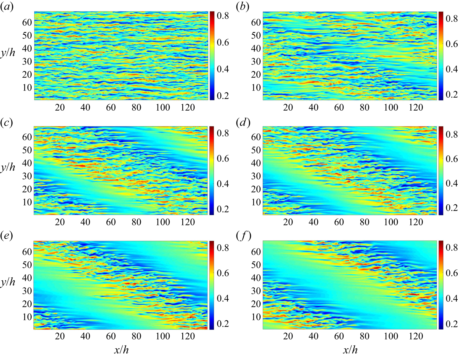
Figure 4. Streamwise velocity (![]() $u$) at the midgap location (
$u$) at the midgap location (![]() $z=h$) for d-type roughness at (a)
$z=h$) for d-type roughness at (a) ![]() $Re=500$, (b)
$Re=500$, (b) ![]() $Re=450$, (c)
$Re=450$, (c) ![]() $Re=425$, (d)
$Re=425$, (d) ![]() $Re=400$, (e)
$Re=400$, (e) ![]() $Re=375$ and (f)
$Re=375$ and (f) ![]() $Re=350$.
$Re=350$.

Figure 5. Streamwise velocity (![]() $u$) at the midgap location (
$u$) at the midgap location (![]() $z=h$) for k-type roughness at (a)
$z=h$) for k-type roughness at (a) ![]() $Re=500$, (b)
$Re=500$, (b) ![]() $Re=350$, (c)
$Re=350$, (c) ![]() $Re=325$ and (d)
$Re=325$ and (d) ![]() $Re=300$.
$Re=300$.
The smooth pCf is known to have stable bands for Reynolds numbers in the range ![]() $Re \in [325,400]$ (Ishida et al. Reference Ishida, Brethouwer, Duguet and Tsukahara2017; Gokul & Narasimhamurthy Reference Gokul and Narasimhamurthy2022). Compared with the smooth pCf, the transitional range for the k-type roughness has shifted downwards (
$Re \in [325,400]$ (Ishida et al. Reference Ishida, Brethouwer, Duguet and Tsukahara2017; Gokul & Narasimhamurthy Reference Gokul and Narasimhamurthy2022). Compared with the smooth pCf, the transitional range for the k-type roughness has shifted downwards (![]() $Re \in [300,325]$), and the corresponding range for the d-type roughness has moved upwards (
$Re \in [300,325]$), and the corresponding range for the d-type roughness has moved upwards (![]() $Re \in [350,425]$). We need to understand why the roughness causes a shift in the transitional range. The streamwise vorticity plays a crucial role in the formation and sustenance of the elongated streaks that constitute the turbulent bands. The regeneration cycle proposed by Hamilton et al. (Reference Hamilton, Kim and Waleffe1995) thoroughly explains this relationship in the smooth pCf. The streamwise vorticity decays as it produces the elongated streaks through a redistribution of momentum (lift-up effect). The streaks thus formed develop a waviness and eventually break down, releasing vorticity in all three directions, which also regenerates the streamwise vorticity. The reenergised streamwise vorticity will again form elongated streaks, thus completing a cycle. However, the roughness elements interfere with the near-wall flow dynamics and modify the regeneration cycle, most likely weakening it (Jiménez Reference Jiménez2004). Therefore, the roughness should offer an additional mechanism for regenerating the streamwise vorticity. Figure 6 shows the streamwise vorticity in an
$Re \in [350,425]$). We need to understand why the roughness causes a shift in the transitional range. The streamwise vorticity plays a crucial role in the formation and sustenance of the elongated streaks that constitute the turbulent bands. The regeneration cycle proposed by Hamilton et al. (Reference Hamilton, Kim and Waleffe1995) thoroughly explains this relationship in the smooth pCf. The streamwise vorticity decays as it produces the elongated streaks through a redistribution of momentum (lift-up effect). The streaks thus formed develop a waviness and eventually break down, releasing vorticity in all three directions, which also regenerates the streamwise vorticity. The reenergised streamwise vorticity will again form elongated streaks, thus completing a cycle. However, the roughness elements interfere with the near-wall flow dynamics and modify the regeneration cycle, most likely weakening it (Jiménez Reference Jiménez2004). Therefore, the roughness should offer an additional mechanism for regenerating the streamwise vorticity. Figure 6 shows the streamwise vorticity in an ![]() $x$–
$x$–![]() $z$ plane at the midspan location for the current rough pCf cases within the transitional regime. In the k-type roughness, vortices are generated within the cavities and are eventually shed from the roughness elements into the outer flow. On the other hand, the d-type roughness does not exhibit the same type of vortex shedding as the k-type roughness. The stable vortices in the cavities of the d-type roughness (to be discussed in conjunction with figure 13(a), presented later) act as a deterrent to vortex shedding (Perry et al. Reference Perry, Schofield and Joubert1969; Coleman et al. Reference Coleman, Nikora, McLean and Schlicke2007). However, not all turbulent events near the cavities can be ruled out, as there can be occasional ejections (Townsend Reference Townsend1976). Jiménez (Reference Jiménez2004) and Leonardi et al. (Reference Leonardi, Orlandi, Djenidi and Antonia2004) also confirmed the occurrence of ejections from the cavities of the d-type roughness. However, the intensity of these events is lower than that observed in the k-type roughness (Leonardi et al. Reference Leonardi, Orlandi and Antonia2007). Even if we account for these events in the d-type roughness, given their sporadic and weak nature, their contribution to vorticity regeneration is likely insignificant. In contrast, the ribs in the k-type roughness act as vortex generators and function as an alternate source for streamwise vorticity regeneration. Therefore, the k-type roughness can sustain stable laminar–turbulent bands at lower Reynolds numbers than the d-type roughness and the smooth pCf. However, the d-type roughness causing an upwards shift in the transitional range compared with the smooth pCf can come across as a surprise. Choi & Fujisawa (Reference Choi and Fujisawa1993) studied the development of a zero-pressure-gradient turbulent boundary layer over a flat plate with a square cavity similar to that in a d-type roughness. They found that the stable recirculation zone in the cavity alters the near-wall flow dynamics, which reduces the incidence of turbulent events compared with a smooth boundary layer. Therefore, exploring the vortical structures within the near-wall region can provide further insights. Figures 7(a) and 7(b) shows the isosurfaces of
$z$ plane at the midspan location for the current rough pCf cases within the transitional regime. In the k-type roughness, vortices are generated within the cavities and are eventually shed from the roughness elements into the outer flow. On the other hand, the d-type roughness does not exhibit the same type of vortex shedding as the k-type roughness. The stable vortices in the cavities of the d-type roughness (to be discussed in conjunction with figure 13(a), presented later) act as a deterrent to vortex shedding (Perry et al. Reference Perry, Schofield and Joubert1969; Coleman et al. Reference Coleman, Nikora, McLean and Schlicke2007). However, not all turbulent events near the cavities can be ruled out, as there can be occasional ejections (Townsend Reference Townsend1976). Jiménez (Reference Jiménez2004) and Leonardi et al. (Reference Leonardi, Orlandi, Djenidi and Antonia2004) also confirmed the occurrence of ejections from the cavities of the d-type roughness. However, the intensity of these events is lower than that observed in the k-type roughness (Leonardi et al. Reference Leonardi, Orlandi and Antonia2007). Even if we account for these events in the d-type roughness, given their sporadic and weak nature, their contribution to vorticity regeneration is likely insignificant. In contrast, the ribs in the k-type roughness act as vortex generators and function as an alternate source for streamwise vorticity regeneration. Therefore, the k-type roughness can sustain stable laminar–turbulent bands at lower Reynolds numbers than the d-type roughness and the smooth pCf. However, the d-type roughness causing an upwards shift in the transitional range compared with the smooth pCf can come across as a surprise. Choi & Fujisawa (Reference Choi and Fujisawa1993) studied the development of a zero-pressure-gradient turbulent boundary layer over a flat plate with a square cavity similar to that in a d-type roughness. They found that the stable recirculation zone in the cavity alters the near-wall flow dynamics, which reduces the incidence of turbulent events compared with a smooth boundary layer. Therefore, exploring the vortical structures within the near-wall region can provide further insights. Figures 7(a) and 7(b) shows the isosurfaces of ![]() $-\lambda _{2}$ for the rough pCf cases within the transitional regime, providing a visualisation of vortical structures, as defined by Jeong & Hussain (Reference Jeong and Hussain1995) [vortical structures corresponding to a smooth pCf are also shown in figure 7(c) for comparison]. Here
$-\lambda _{2}$ for the rough pCf cases within the transitional regime, providing a visualisation of vortical structures, as defined by Jeong & Hussain (Reference Jeong and Hussain1995) [vortical structures corresponding to a smooth pCf are also shown in figure 7(c) for comparison]. Here ![]() $\lambda _{2}$ is defined as the second largest eigenvalue of the tensor
$\lambda _{2}$ is defined as the second largest eigenvalue of the tensor ![]() $\boldsymbol{\mathsf{S}}^{2}+\boldsymbol{\mathsf{\Omega}}^{2}$, where
$\boldsymbol{\mathsf{S}}^{2}+\boldsymbol{\mathsf{\Omega}}^{2}$, where ![]() $\boldsymbol{\mathsf{S}}$ and
$\boldsymbol{\mathsf{S}}$ and ![]() $\boldsymbol{\mathsf{\Omega}}$ are the symmetric and antisymmetric parts of the velocity gradient tensor, respectively. A closer examination of the near-wall structures shows a clear distinction between the rough pCf cases. Also note the striking similarity between the k-type roughness and the smooth pCf. In the d-type roughness, the near-wall region is dominated by vortical structures oriented in the spanwise direction. Compared with the k-type roughness and the smooth pCf, the streamwise-oriented vortical structures in the d-type roughness are away from the stationary wall, resulting in a relatively stable region close to the wall. Luchini, Manzo & Pozzi (Reference Luchini, Manzo and Pozzi1991) have attributed the drag-reducing nature of riblets to a similar shift of the turbulent structures away from the wall. This could lead to reduced disturbances and increased stability near the stationary wall, which can negatively affect the formation and sustenance of streaks. Consequently, the d-type roughness cannot sustain the elongated streaks that constitute the turbulent bands as effectively as the smooth pCf. As a result, the flow in the d-type roughness laminarises at a higher Reynolds number than the smooth pCf.
$\boldsymbol{\mathsf{\Omega}}$ are the symmetric and antisymmetric parts of the velocity gradient tensor, respectively. A closer examination of the near-wall structures shows a clear distinction between the rough pCf cases. Also note the striking similarity between the k-type roughness and the smooth pCf. In the d-type roughness, the near-wall region is dominated by vortical structures oriented in the spanwise direction. Compared with the k-type roughness and the smooth pCf, the streamwise-oriented vortical structures in the d-type roughness are away from the stationary wall, resulting in a relatively stable region close to the wall. Luchini, Manzo & Pozzi (Reference Luchini, Manzo and Pozzi1991) have attributed the drag-reducing nature of riblets to a similar shift of the turbulent structures away from the wall. This could lead to reduced disturbances and increased stability near the stationary wall, which can negatively affect the formation and sustenance of streaks. Consequently, the d-type roughness cannot sustain the elongated streaks that constitute the turbulent bands as effectively as the smooth pCf. As a result, the flow in the d-type roughness laminarises at a higher Reynolds number than the smooth pCf.

Figure 6. Instantaneous streamwise vorticity (![]() $\omega _{x}$) in an
$\omega _{x}$) in an ![]() $x$–
$x$–![]() $z$ plane at
$z$ plane at ![]() $y=34h$ for (a) d-type roughness (
$y=34h$ for (a) d-type roughness (![]() $Re=350$) and (b) k-type roughness (
$Re=350$) and (b) k-type roughness (![]() $Re=300$). Vorticity values are normalised by
$Re=300$). Vorticity values are normalised by ![]() ${U_{w}}^{2}/\nu$.
${U_{w}}^{2}/\nu$.
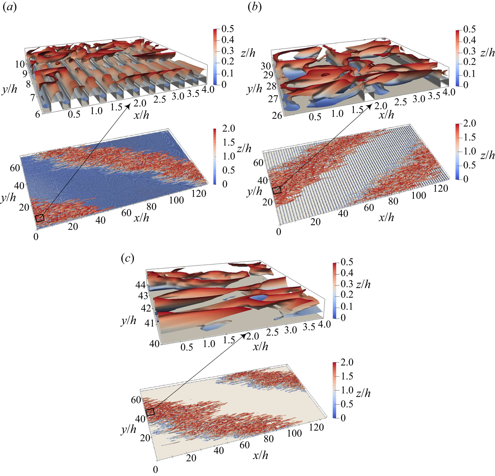
Figure 7. Isosurface of ![]() $\lambda _{2}=-1 \times 10^{-8}$ coloured with the variation in
$\lambda _{2}=-1 \times 10^{-8}$ coloured with the variation in ![]() $z/h$ for (a) d-type roughness (
$z/h$ for (a) d-type roughness (![]() $Re=350$), (b) k-type roughness (
$Re=350$), (b) k-type roughness (![]() $Re=300$) and (c) smooth pCf (
$Re=300$) and (c) smooth pCf (![]() $Re=325$). Here
$Re=325$). Here ![]() $\lambda _{2}$ values are normalised using
$\lambda _{2}$ values are normalised using ![]() ${U_{w}}^{4}/\nu ^{2}$. Top panels show enlarged views of a small region (shown by arrows).
${U_{w}}^{4}/\nu ^{2}$. Top panels show enlarged views of a small region (shown by arrows).
The pattern of laminar–turbulent bands is periodic in the streamwise and spanwise directions. It has large wavelengths in both these directions. The experiments by Prigent et al. (Reference Prigent, Grégoire, Chaté and Dauchot2003) suggest that these wavelengths are sensitive to changes in Reynolds number. However, the pattern wavelengths obtained for the rough pCf cases in the present study remain unchanged with the Reynolds number. We have also observed this phenomenon in our previous study on the smooth pCf (Gokul & Narasimhamurthy Reference Gokul and Narasimhamurthy2022). The wavelengths ![]() $\lambda _{x}$ and
$\lambda _{x}$ and ![]() $\lambda _{y}$ are always equal to the domain dimensions
$\lambda _{y}$ are always equal to the domain dimensions ![]() $L_{x}$ and
$L_{x}$ and ![]() $L_{y}$, respectively, due to the influence of the periodic boundary condition. This phenomenon is inevitable in numerical simulations not performed in large-aspect-ratio systems. The transition study by Ishida et al. (Reference Ishida, Brethouwer, Duguet and Tsukahara2017), who used a similar domain as ours, also observed the same. Tsukahara, Kawaguchi & Kawamura (Reference Tsukahara, Kawaguchi and Kawamura2009) used a much larger domain and found their wavelengths remain unchanged with Reynolds number due to the influence of periodic boundary conditions. As the pattern wavelengths for rough pCf cases in the present study are equal to the corresponding domain dimensions, the pattern will consistently align with one of the domain diagonals. Therefore, the angle made by the pattern (with
$L_{y}$, respectively, due to the influence of the periodic boundary condition. This phenomenon is inevitable in numerical simulations not performed in large-aspect-ratio systems. The transition study by Ishida et al. (Reference Ishida, Brethouwer, Duguet and Tsukahara2017), who used a similar domain as ours, also observed the same. Tsukahara, Kawaguchi & Kawamura (Reference Tsukahara, Kawaguchi and Kawamura2009) used a much larger domain and found their wavelengths remain unchanged with Reynolds number due to the influence of periodic boundary conditions. As the pattern wavelengths for rough pCf cases in the present study are equal to the corresponding domain dimensions, the pattern will consistently align with one of the domain diagonals. Therefore, the angle made by the pattern (with ![]() $x$ direction) in the d-type and the k-type roughness is approximately equal to
$x$ direction) in the d-type and the k-type roughness is approximately equal to ![]() $27^{\circ }$. The pattern angle in the smooth pCf is the same as that of the rough pCf cases.
$27^{\circ }$. The pattern angle in the smooth pCf is the same as that of the rough pCf cases.
Large-scale flow is key in understanding the obliqueness of the laminar–turbulent bands. It is responsible for advecting the streaks in the turbulent spots in an oblique fashion, which later develop to form oblique bands (Duguet & Schlatter Reference Duguet and Schlatter2013). There is a pronounced scale separation between the turbulent fluctuations that constitute the streaks and the large-scale flow associated with the laminar–turbulent bands (Gomé, Tuckerman & Barkley Reference Gomé, Tuckerman and Barkley2023a). A low-pass filter can extract the large scales linked to the pattern (Ishida, Duguet & Tsukahara Reference Ishida, Duguet and Tsukahara2017; Tsukahara et al. Reference Tsukahara, Tomioka, Ishida, Duguet and Brethouwer2018). Figure 8 shows wall-normal averaged large-scale flow vectors (obtained through low-pass filtering) along with the contours of streamwise velocity fluctuations (![]() ${u}'=u-\bar {u}$, where
${u}'=u-\bar {u}$, where ![]() $\bar {u}$ is the mean streamwise velocity obtained by time averaging) in the background for the d-type and the k-type roughness. The flow is parallel to the oblique bands near the laminar–turbulent boundaries, implying a significant spanwise velocity component in the large-scale flow. The probability density function of the angle
$\bar {u}$ is the mean streamwise velocity obtained by time averaging) in the background for the d-type and the k-type roughness. The flow is parallel to the oblique bands near the laminar–turbulent boundaries, implying a significant spanwise velocity component in the large-scale flow. The probability density function of the angle ![]() $\beta$ made by the large-scale flow vectors (with
$\beta$ made by the large-scale flow vectors (with ![]() $x$ direction) is shown in figure 9. The peak probability for the d-type and the k-type roughness is at
$x$ direction) is shown in figure 9. The peak probability for the d-type and the k-type roughness is at ![]() $24^{\circ }$, which matches well with the pattern angle.
$24^{\circ }$, which matches well with the pattern angle.

Figure 8. Streamwise velocity fluctuations (![]() $u^{\prime }$) at the midgap location (
$u^{\prime }$) at the midgap location (![]() $z=h$) and the corresponding wall-normal-averaged large-scale flow (
$z=h$) and the corresponding wall-normal-averaged large-scale flow (![]() $\bar {U}, \bar {V}$) for (a) d-type roughness (
$\bar {U}, \bar {V}$) for (a) d-type roughness (![]() $Re=350$) and (b) k-type roughness (
$Re=350$) and (b) k-type roughness (![]() $Re=300$).
$Re=300$).
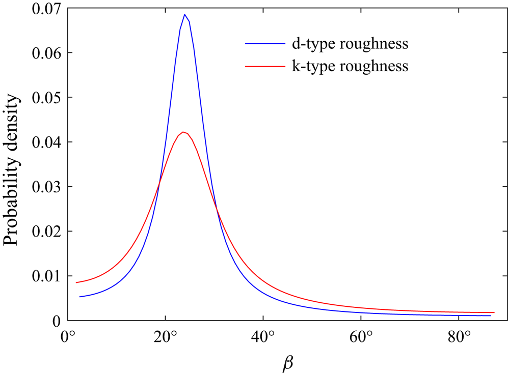
Figure 9. Probability distribution function of angle ![]() $\beta$ made by the large-scale flow vectors. The probability density gives the likelihood associated with various orientations of the large-scale flow vectors.
$\beta$ made by the large-scale flow vectors. The probability density gives the likelihood associated with various orientations of the large-scale flow vectors.
The transition to turbulence in pCf is spatiotemporal (Philip & Manneville Reference Philip and Manneville2011). Spatiotemporal diagrams (figures 10 and 11) help understand the dynamics of laminar–turbulent bands. This diagram represents data recorded across both space and time. The time series data of streamwise velocity ![]() $u$ are collected at 288 equidistant points along a spanwise line located at the centre of the domain (
$u$ are collected at 288 equidistant points along a spanwise line located at the centre of the domain (![]() $x=68h$,
$x=68h$, ![]() $z=h$) for a total time of
$z=h$) for a total time of ![]() $1000 h/U_{w}$. The spatiotemporal data are recorded after a stable pattern has emerged to avoid the initial transients in the flow. The laminar–turbulent coexistence in the spatiotemporal plane also yields oblique bands like a streamwise–spanwise (
$1000 h/U_{w}$. The spatiotemporal data are recorded after a stable pattern has emerged to avoid the initial transients in the flow. The laminar–turbulent coexistence in the spatiotemporal plane also yields oblique bands like a streamwise–spanwise (![]() $x$–
$x$–![]() $y$) plane. The effect of the Reynolds number on the spatiotemporal dynamics is such that there is a reduction in the area occupied by the turbulent regions as the Reynolds number is reduced. This reduction in the turbulent area indicates flow being turbulent at fewer points and for lesser duration of time. The frequency of the pattern in the spatiotemporal plane is found using a fast Fourier transform (FFT). Figure 12 shows the spectral analysis for the rough pCf cases. The most energetic frequencies associated with the pattern for the d-type and the k-type roughness are
$y$) plane. The effect of the Reynolds number on the spatiotemporal dynamics is such that there is a reduction in the area occupied by the turbulent regions as the Reynolds number is reduced. This reduction in the turbulent area indicates flow being turbulent at fewer points and for lesser duration of time. The frequency of the pattern in the spatiotemporal plane is found using a fast Fourier transform (FFT). Figure 12 shows the spectral analysis for the rough pCf cases. The most energetic frequencies associated with the pattern for the d-type and the k-type roughness are ![]() $3.81 \times 10^{-3}$ and
$3.81 \times 10^{-3}$ and ![]() $3.05 \times 10^{-3}$, respectively. The corresponding time period can be found by taking the reciprocal of peak frequency. Therefore, the time period of the pattern in the d-type and the k-type roughness are
$3.05 \times 10^{-3}$, respectively. The corresponding time period can be found by taking the reciprocal of peak frequency. Therefore, the time period of the pattern in the d-type and the k-type roughness are ![]() $262.14 h/U_{w}$ and
$262.14 h/U_{w}$ and ![]() $327.67 h/U_{w}$, respectively. The peak frequency and time period do not change with the Reynolds number within the transitional regime. Having the wavelength (
$327.67 h/U_{w}$, respectively. The peak frequency and time period do not change with the Reynolds number within the transitional regime. Having the wavelength (![]() $\lambda _{x} \approx 136h$) and frequency already established, one can ascertain the speed of the wave in the
$\lambda _{x} \approx 136h$) and frequency already established, one can ascertain the speed of the wave in the ![]() $x$ direction. The calculated wave speeds for the d-type and the k-type roughness are approximately
$x$ direction. The calculated wave speeds for the d-type and the k-type roughness are approximately ![]() $0.52 U_{w}$ and
$0.52 U_{w}$ and ![]() $0.41 U_{w}$, respectively. It is interesting to note that these speeds compares well with the respective mean streamwise velocities at the apparent midgap locations of the rough pCf cases (the locations of apparent midgaps and their corresponding mean streamwise velocities are shown in Appendix A.2). Similarly, the mean band speed in the smooth pCf closely matches the mean streamwise velocity in the midgap (Gokul & Narasimhamurthy Reference Gokul and Narasimhamurthy2022).
$0.41 U_{w}$, respectively. It is interesting to note that these speeds compares well with the respective mean streamwise velocities at the apparent midgap locations of the rough pCf cases (the locations of apparent midgaps and their corresponding mean streamwise velocities are shown in Appendix A.2). Similarly, the mean band speed in the smooth pCf closely matches the mean streamwise velocity in the midgap (Gokul & Narasimhamurthy Reference Gokul and Narasimhamurthy2022).

Figure 10. Streamwise velocity fluctuations (![]() $u^{\prime }$) in a spatiotemporal plane for d-type roughness at (a)
$u^{\prime }$) in a spatiotemporal plane for d-type roughness at (a) ![]() $Re=425$, (b)
$Re=425$, (b) ![]() $Re=400$, (c)
$Re=400$, (c) ![]() $Re=375$ and (d)
$Re=375$ and (d) ![]() $Re=350$.
$Re=350$.

Figure 11. Streamwise velocity fluctuations (![]() $u^{\prime }$) in a spatiotemporal plane for k-type roughness at (a)
$u^{\prime }$) in a spatiotemporal plane for k-type roughness at (a) ![]() $Re=325$ and (b)
$Re=325$ and (b) ![]() $Re=300$.
$Re=300$.
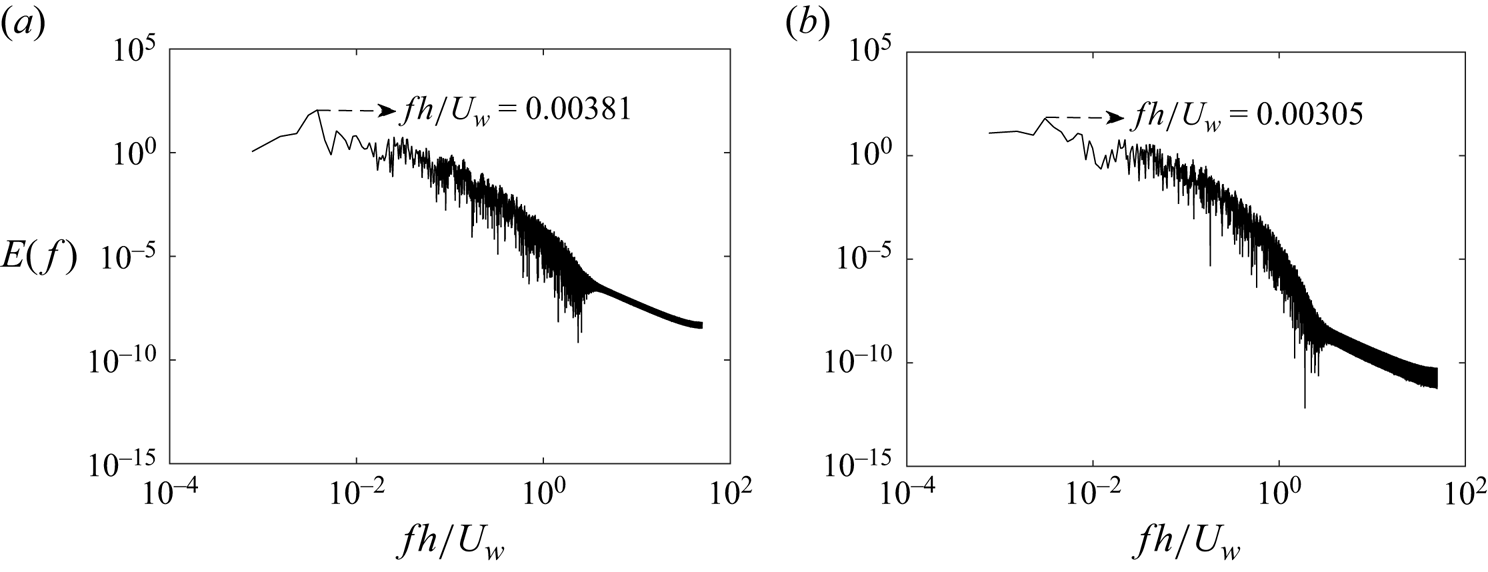
Figure 12. Frequency-based representation of streamwise velocity ![]() $u$ for (a) d-type roughness (
$u$ for (a) d-type roughness (![]() $Re=350$) and (b) k-type roughness (
$Re=350$) and (b) k-type roughness (![]() $Re=300$).
$Re=300$).
In the subsequent analysis, our focus is on exploring the mean flow characteristics of the rough pCf cases. In the transitional regime, the mean quantities have contributions from the turbulent and quasi-laminar regions of the flow field. This aspect is crucial when interpreting the mean quantities in the transitional regime. In the rough pCf cases, data are averaged across pitches, in addition to averaging over time and the ![]() $y$-direction. Figure 13 illustrates the mean streamlines for the near-wall region superimposed on the contours of mean streamwise velocity for the transitional regime. The narrow cavity in the d-type roughness forms a single recirculation zone. This vortex is stable (Perry et al. Reference Perry, Schofield and Joubert1969) and thus shields the outer flow from interacting with the wall or cavity floor in the d-type case. The vortex is relatively weak (Leonardi et al. Reference Leonardi, Orlandi and Antonia2007), resembling a low-velocity, 2-D, lid-driven cavity flow (Cui, Patel & Lin Reference Cui, Patel and Lin2003). Therefore, the mean streamwise velocity within the cavity is significantly lower compared with that of the outer flow. The corresponding friction coefficient (
$y$-direction. Figure 13 illustrates the mean streamlines for the near-wall region superimposed on the contours of mean streamwise velocity for the transitional regime. The narrow cavity in the d-type roughness forms a single recirculation zone. This vortex is stable (Perry et al. Reference Perry, Schofield and Joubert1969) and thus shields the outer flow from interacting with the wall or cavity floor in the d-type case. The vortex is relatively weak (Leonardi et al. Reference Leonardi, Orlandi and Antonia2007), resembling a low-velocity, 2-D, lid-driven cavity flow (Cui, Patel & Lin Reference Cui, Patel and Lin2003). Therefore, the mean streamwise velocity within the cavity is significantly lower compared with that of the outer flow. The corresponding friction coefficient (![]() $C_{f}=\nu ({\partial \bar {u}}/{\partial z})/U_{w}^{2}$) on the cavity floor is negligible, indicating that the wall shear stress is practically zero (see figure 14a). This resembles a free-slip boundary, which can likely contribute to the stability of the recirculation zone within the cavity in the d-type roughness. In contrast,
$C_{f}=\nu ({\partial \bar {u}}/{\partial z})/U_{w}^{2}$) on the cavity floor is negligible, indicating that the wall shear stress is practically zero (see figure 14a). This resembles a free-slip boundary, which can likely contribute to the stability of the recirculation zone within the cavity in the d-type roughness. In contrast, ![]() $C_{f}$ is non-zero on the rib crest. Therefore, the near-wall flow in the d-type case experiences alternate free-slip-like (on the cavity floor) and no-slip (on the rib crest) conditions along the
$C_{f}$ is non-zero on the rib crest. Therefore, the near-wall flow in the d-type case experiences alternate free-slip-like (on the cavity floor) and no-slip (on the rib crest) conditions along the ![]() $x$ direction. MacDonald et al. (Reference MacDonald, Ooi, García-Mayoral, Hutchins and Chung2018) drew an analogy between the mean flow over the d-type roughness and superhydrophobic surfaces, where liquid flows over gas-filled cavities between roughness elements, presenting alternating zero-shear/zero-velocity conditions. This analogy implies that, similar to superhydrophobic surfaces where the liquid skims past the cavities, there is limited interaction between the outer flow and the cavities in the d-type roughness. In the k-type roughness, the flow separates near the trailing edge of the rib and later reattaches to the cavity floor, forming a large vortex near the trailing face and a smaller vortex close to the leading face of the next rib. These vortices are unstable and lead to significant vortex shedding above the rib crests (Perry et al. Reference Perry, Schofield and Joubert1969). The mean streamwise velocity within the cavity is higher than that of the d-type roughness as the ribs are subjected to the outer flow. The
$x$ direction. MacDonald et al. (Reference MacDonald, Ooi, García-Mayoral, Hutchins and Chung2018) drew an analogy between the mean flow over the d-type roughness and superhydrophobic surfaces, where liquid flows over gas-filled cavities between roughness elements, presenting alternating zero-shear/zero-velocity conditions. This analogy implies that, similar to superhydrophobic surfaces where the liquid skims past the cavities, there is limited interaction between the outer flow and the cavities in the d-type roughness. In the k-type roughness, the flow separates near the trailing edge of the rib and later reattaches to the cavity floor, forming a large vortex near the trailing face and a smaller vortex close to the leading face of the next rib. These vortices are unstable and lead to significant vortex shedding above the rib crests (Perry et al. Reference Perry, Schofield and Joubert1969). The mean streamwise velocity within the cavity is higher than that of the d-type roughness as the ribs are subjected to the outer flow. The ![]() $C_{f}$ along the cavity floor is initially negative due to the large recirculation bubble (see figure 14b). It then shifts to positive upon reattachment and returns to negative due to the small recirculation bubble near the next rib. Further, on the rib crest, the
$C_{f}$ along the cavity floor is initially negative due to the large recirculation bubble (see figure 14b). It then shifts to positive upon reattachment and returns to negative due to the small recirculation bubble near the next rib. Further, on the rib crest, the ![]() $C_{f}$ is at its maximum near the leading edge and gradually reduces along its length. The mean velocity profiles for the rough pCf cases in the transitional regime are shown in figure 15. The mean velocity values are plotted at the midcavity (I) and midrib (II) locations and compared with those from the smooth pCf. It is well known that the variation of mean streamwise velocity
$C_{f}$ is at its maximum near the leading edge and gradually reduces along its length. The mean velocity profiles for the rough pCf cases in the transitional regime are shown in figure 15. The mean velocity values are plotted at the midcavity (I) and midrib (II) locations and compared with those from the smooth pCf. It is well known that the variation of mean streamwise velocity ![]() $\bar {u}$ has the typical S-shape in the smooth pCf. Compared with the smooth pCf,
$\bar {u}$ has the typical S-shape in the smooth pCf. Compared with the smooth pCf, ![]() $\bar {u}$ in rough pCf cases is reduced due to the blockage offered by the roughness. This reduction in the magnitude of
$\bar {u}$ in rough pCf cases is reduced due to the blockage offered by the roughness. This reduction in the magnitude of ![]() $\bar {u}$ is more pronounced near the rib-roughened stationary wall and reduces as we approach the smooth moving wall. The
$\bar {u}$ is more pronounced near the rib-roughened stationary wall and reduces as we approach the smooth moving wall. The ![]() $\bar {u}$ variations at I and II locations follow distinct paths close to the stationary wall but collapse beyond
$\bar {u}$ variations at I and II locations follow distinct paths close to the stationary wall but collapse beyond ![]() $z=0.5h$ in the d-type roughness. However, in the k-type roughness, the
$z=0.5h$ in the d-type roughness. However, in the k-type roughness, the ![]() $\bar {u}$ variations at I and II follow different paths until the channel centre (
$\bar {u}$ variations at I and II follow different paths until the channel centre (![]() $z=h$) before collapsing.
$z=h$) before collapsing.

Figure 13. Mean streamlines with contours of mean streamwise velocity in the background for (a) d-type roughness (![]() $Re=350$) and (b) k-type roughness (
$Re=350$) and (b) k-type roughness (![]() $Re=300$). Here,
$Re=300$). Here, ![]() $x$ is normalised by the pitch
$x$ is normalised by the pitch ![]() $\lambda$ instead of
$\lambda$ instead of ![]() $h$.
$h$.
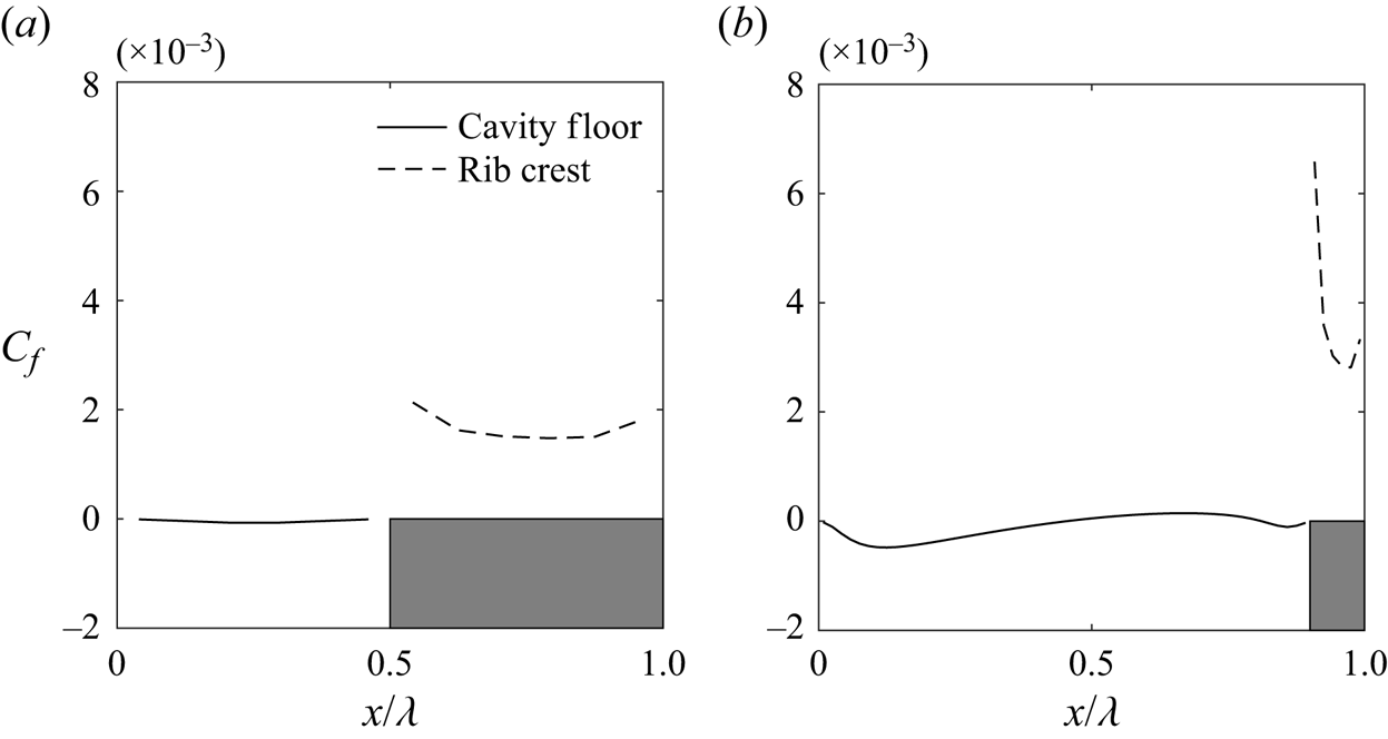
Figure 14. Variation of skin friction coefficient on the cavity floor and rib crest for (a) d-type roughness (![]() $Re=350$) and (b) k-type roughness (
$Re=350$) and (b) k-type roughness (![]() $Re=300$). Here,
$Re=300$). Here, ![]() $x$ is normalised by the pitch
$x$ is normalised by the pitch ![]() $\lambda$ instead of
$\lambda$ instead of ![]() $h$.
$h$.
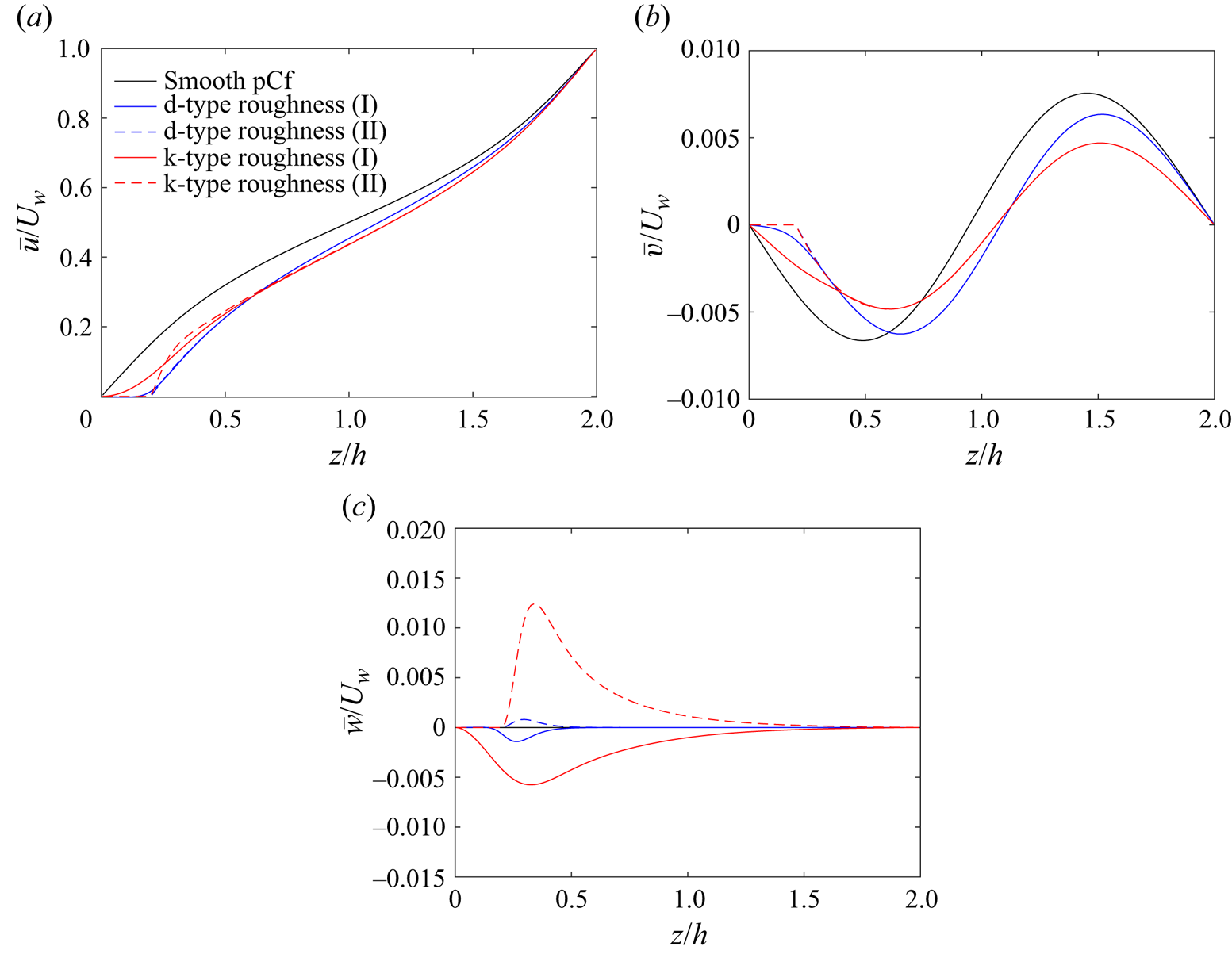
Figure 15. Variation of (a) mean streamwise velocity ![]() $\bar {u}$, (b) mean spanwise velocity
$\bar {u}$, (b) mean spanwise velocity ![]() $\bar {v}$ and (c) mean wall-normal velocity
$\bar {v}$ and (c) mean wall-normal velocity ![]() $\bar {w}$ along the wall-normal direction for d-type roughness and k-type roughness at the midcavity (I) and midrib (II) locations at a Reynolds number close to their lower threshold (
$\bar {w}$ along the wall-normal direction for d-type roughness and k-type roughness at the midcavity (I) and midrib (II) locations at a Reynolds number close to their lower threshold (![]() $Re_{g}$). Here
$Re_{g}$). Here ![]() $Re_{g}$ is the Reynolds number in the transitional regime below which the flow turns laminar. Corresponding velocity profiles in smooth pCf are also plotted for comparison.
$Re_{g}$ is the Reynolds number in the transitional regime below which the flow turns laminar. Corresponding velocity profiles in smooth pCf are also plotted for comparison.
Table 3 presents the values of friction velocity ![]() $u_{\tau }$ and the corresponding friction Reynolds number
$u_{\tau }$ and the corresponding friction Reynolds number ![]() $Re_{\tau }$ for the d-type and the k-type roughness (the corresponding values for the smooth pCf are also given for comparison). Note that the friction velocity for the rib-roughened wall is due to both the viscous drag and the pressure drag. The method used to calculate the friction velocity for the rough wall is the same as that of Mahmoodi-Jezeh & Wang (Reference Mahmoodi-Jezeh and Wang2020). When compared, the friction velocity
$Re_{\tau }$ for the d-type and the k-type roughness (the corresponding values for the smooth pCf are also given for comparison). Note that the friction velocity for the rib-roughened wall is due to both the viscous drag and the pressure drag. The method used to calculate the friction velocity for the rough wall is the same as that of Mahmoodi-Jezeh & Wang (Reference Mahmoodi-Jezeh and Wang2020). When compared, the friction velocity ![]() $u_{\tau }$ at a particular Reynolds number is the highest in the k-type roughness. The enhanced friction in the k-type roughness promotes more turbulence generation compared with the d-type roughness and the smooth pCf, allowing it to sustain stable laminar–turbulent bands at lower Reynolds numbers than the other two cases. The values of
$u_{\tau }$ at a particular Reynolds number is the highest in the k-type roughness. The enhanced friction in the k-type roughness promotes more turbulence generation compared with the d-type roughness and the smooth pCf, allowing it to sustain stable laminar–turbulent bands at lower Reynolds numbers than the other two cases. The values of ![]() $u_{\tau }$ for the d-type roughness closely resemble that of the smooth pCf, exhibiting only a marginal difference. Thereby, the d-type roughness seems to fail to induce greater turbulence generation compared with the smooth pCf.
$u_{\tau }$ for the d-type roughness closely resemble that of the smooth pCf, exhibiting only a marginal difference. Thereby, the d-type roughness seems to fail to induce greater turbulence generation compared with the smooth pCf.
Table 3. Friction velocity (![]() $u_{\tau }$) and friction Reynolds number (
$u_{\tau }$) and friction Reynolds number (![]() $Re_{\tau }$) for the three cases considered in the present study.
$Re_{\tau }$) for the three cases considered in the present study. ![]() $\overline {V_{d}}$ and
$\overline {V_{d}}$ and ![]() $\overline {P_{d}}$ are viscous and pressure drags whereas the subscripts
$\overline {P_{d}}$ are viscous and pressure drags whereas the subscripts ![]() $S$ and
$S$ and ![]() $M$ refer to the stationary and moving walls, respectively. The symbols
$M$ refer to the stationary and moving walls, respectively. The symbols ![]() $u_{\tau }$ and
$u_{\tau }$ and ![]() $Re_{\tau }$ are also used to refer to the global friction velocity
$Re_{\tau }$ are also used to refer to the global friction velocity ![]() $(u_{\tau }=\sqrt {({u_{\tau S}^{2}+u_{\tau M}^{2}})/{2}})$ and the corresponding global friction Reynolds number (
$(u_{\tau }=\sqrt {({u_{\tau S}^{2}+u_{\tau M}^{2}})/{2}})$ and the corresponding global friction Reynolds number (![]() $Re_{\tau }=u_{\tau }h/\nu$), respectively.
$Re_{\tau }=u_{\tau }h/\nu$), respectively.

Unlike the turbulent regime, ![]() $\bar {v}$ is not negligible in the transitional regime (see figure 15b). In the smooth pCf, the magnitude of
$\bar {v}$ is not negligible in the transitional regime (see figure 15b). In the smooth pCf, the magnitude of ![]() $\bar {v}$ is zero at the stationary wall, increases to a negative peak and then drops to zero near the channel centre (
$\bar {v}$ is zero at the stationary wall, increases to a negative peak and then drops to zero near the channel centre (![]() $z=h$). At
$z=h$). At ![]() $z=h$,
$z=h$, ![]() $\bar {v}$ changes sign, increases to a positive peak before falling to zero at the moving wall. The
$\bar {v}$ changes sign, increases to a positive peak before falling to zero at the moving wall. The ![]() $\bar {v}$ variation in the rough pCf cases also exhibits a similar trend, except that, unlike the smooth pCf, the shift in sign occurs slightly away from the centre of the channel.
$\bar {v}$ variation in the rough pCf cases also exhibits a similar trend, except that, unlike the smooth pCf, the shift in sign occurs slightly away from the centre of the channel.
The mean wall-normal velocity ![]() $\bar {w}$ is not zero in the rough pCf cases as in the smooth pCf (see figure 15c). The
$\bar {w}$ is not zero in the rough pCf cases as in the smooth pCf (see figure 15c). The ![]() $\bar {w}$ is non-zero near the ribs for the d-type roughness and becomes negligible beyond
$\bar {w}$ is non-zero near the ribs for the d-type roughness and becomes negligible beyond ![]() $z=0.5h$. However, in the k-type roughness,
$z=0.5h$. However, in the k-type roughness, ![]() $\bar {w}$ is predominantly non-zero and diminishes only close to the smooth-moving wall. In the d-type and the k-type roughness,
$\bar {w}$ is predominantly non-zero and diminishes only close to the smooth-moving wall. In the d-type and the k-type roughness, ![]() $\bar {w}$ varies in the
$\bar {w}$ varies in the ![]() $-z$ direction at location I due to the fluid entering the cavities. At location II,
$-z$ direction at location I due to the fluid entering the cavities. At location II, ![]() $\bar {w}$ varies along the
$\bar {w}$ varies along the ![]() $+z$ direction for both the rough cases due to the upwards deflection of the flow near the rib crests. The
$+z$ direction for both the rough cases due to the upwards deflection of the flow near the rib crests. The ![]() $\bar {w}$ values in the d-type roughness are much smaller than its k-type counterpart as the effect of roughness on the outer flow is very limited in the former.
$\bar {w}$ values in the d-type roughness are much smaller than its k-type counterpart as the effect of roughness on the outer flow is very limited in the former.
It is generally acknowledged that the secondary flow in the smooth pCf consists of counter-rotating secondary vortices (also known as roll cells) when the flow is turbulent. These vortices are critical in sustaining the elongated streaks in the turbulent flow (Hamilton et al. Reference Hamilton, Kim and Waleffe1995). Javanappa & Narasimhamurthy (Reference Javanappa and Narasimhamurthy2021) were one of the first to report counter-rotating secondary vortices in rough turbulent Couette flows. Similarly, the secondary streamlines for the rough pCf cases in the present study reveal the presence of roll cells in the turbulent regime (see figure 16). Figure 17 shows the mean secondary flow streamlines for the rough pCf cases in the transitional regime. The counter-rotating vortices are not visible in the mean secondary flow. On the contrary, co-rotating vortices confined to the channel centre are observed. Examining the instantaneous fields is necessary before confirming the absence of the counter-rotating vortices in the transitional regime. Figure 18 shows the contours of instantaneous wall-normal velocity ![]() $w$ for the d-type and the k-type roughness in a
$w$ for the d-type and the k-type roughness in a ![]() $yz$ plane at
$yz$ plane at ![]() $x/h=0.1$ and
$x/h=0.1$ and ![]() $x/h=0.9$, respectively. The changes in the direction of wall-normal velocity denote the existence of counter-rotating vortices in the turbulent region, while the laminar region exhibits an absence of such vortices. These vortices are directly connected to the elongated streaks in the turbulent bands. It is essential to note that the co-rotating vortices are not present in the instantaneous flow field. Therefore, the inference drawn is that the co-rotating vortices in figure 17 result from the averaging process, which includes the characteristics from both turbulent and quasi-laminar regions.
$x/h=0.9$, respectively. The changes in the direction of wall-normal velocity denote the existence of counter-rotating vortices in the turbulent region, while the laminar region exhibits an absence of such vortices. These vortices are directly connected to the elongated streaks in the turbulent bands. It is essential to note that the co-rotating vortices are not present in the instantaneous flow field. Therefore, the inference drawn is that the co-rotating vortices in figure 17 result from the averaging process, which includes the characteristics from both turbulent and quasi-laminar regions.
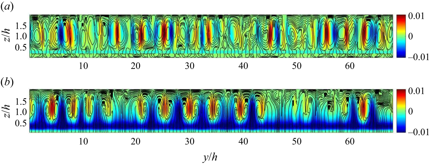
Figure 16. Mean secondary flow streamlines with mean wall-normal velocity in the background at ![]() $Re=500$ for (a) d-type roughness and (b) k-type roughness at midcavity (I) location. The velocities used for generating streamlines and contours are averaged across time and pitches in the
$Re=500$ for (a) d-type roughness and (b) k-type roughness at midcavity (I) location. The velocities used for generating streamlines and contours are averaged across time and pitches in the ![]() $x$ direction.
$x$ direction.
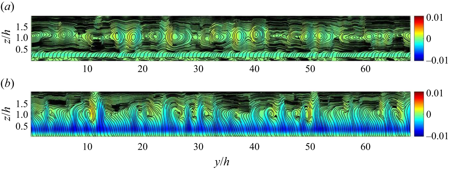
Figure 17. Mean secondary flow streamlines with mean wall-normal velocity in the background for (a) d-type roughness (![]() $Re=350$) and (b) k-type roughness (
$Re=350$) and (b) k-type roughness (![]() $Re=300$) at midcavity (I) location. The velocities used for generating streamlines and contours are averaged across time and pitches in the
$Re=300$) at midcavity (I) location. The velocities used for generating streamlines and contours are averaged across time and pitches in the ![]() $x$ direction.
$x$ direction.

Figure 18. Instantaneous wall-normal velocity ![]() $w$ for (a) d-type roughness (
$w$ for (a) d-type roughness (![]() $Re=350$) at
$Re=350$) at ![]() $x/h=0.1$ and (b) k-type roughness (
$x/h=0.1$ and (b) k-type roughness (![]() $Re=300$) at
$Re=300$) at ![]() $x/h=0.9$.
$x/h=0.9$.
The Reynolds stresses for the rough pCf cases in the transitional regime are shown in figure 19. They are plotted at locations I and II, and the corresponding values in the smooth pCf are also presented. A comparison with the Reynolds stresses in the turbulent regime is also made to highlight the significant differences (see Appendix A for Reynolds stresses in the turbulent regime). In the d-type roughness, beyond ![]() $z=0.5h$, the variations of Reynolds stresses are similar in shape to those in the smooth pCf. However, the curves for the d-type roughness and the smooth pCf never collapse on each other. The mismatch arises because the slope of the curves in the d-type roughness reaches zero at
$z=0.5h$, the variations of Reynolds stresses are similar in shape to those in the smooth pCf. However, the curves for the d-type roughness and the smooth pCf never collapse on each other. The mismatch arises because the slope of the curves in the d-type roughness reaches zero at ![]() $z=1.1h$ rather than at the midgap plane (
$z=1.1h$ rather than at the midgap plane (![]() $z=h$).
$z=h$).
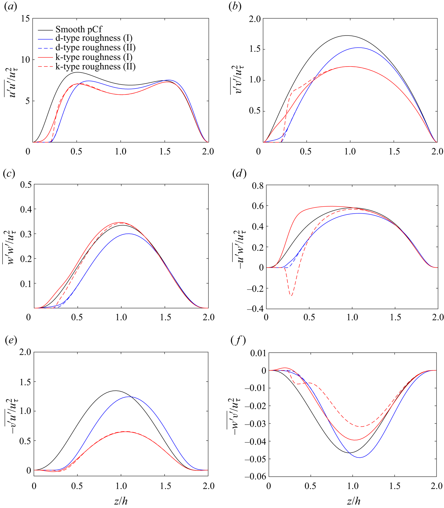
Figure 19. Variation of components of Reynolds stress tensor (a–f) along the wall-normal direction for d-type roughness and k-type roughness at the midcavity (I) and midrib (II) locations at a Reynolds number close to their ![]() $Re_{g}$. Corresponding Reynolds stresses in smooth pCf are also plotted for comparison. The stresses are normalised using the square of global friction velocity
$Re_{g}$. Corresponding Reynolds stresses in smooth pCf are also plotted for comparison. The stresses are normalised using the square of global friction velocity ![]() $u_{\tau }^{2}$ of each case.
$u_{\tau }^{2}$ of each case.
Unlike the d-type roughness, the Reynolds stress profiles in the k-type roughness are significantly different from those in the smooth pCf, especially in the bottom half of the channel. In addition, it is worth emphasising that the Reynolds stresses for the k-type roughness in the transitional and turbulent regimes have specific differences. The ![]() $\overline {u^{\prime }u^{\prime }}$ variation in the k-type roughness has a lower magnitude near the rib-roughened bottom wall compared with the smooth top wall when the flow is turbulent. Interestingly, in the transitional regime, this difference in the magnitude of the peaks in the bottom and top half of the channel diminishes. Similarly, the peak near the rib-roughened bottom wall for the
$\overline {u^{\prime }u^{\prime }}$ variation in the k-type roughness has a lower magnitude near the rib-roughened bottom wall compared with the smooth top wall when the flow is turbulent. Interestingly, in the transitional regime, this difference in the magnitude of the peaks in the bottom and top half of the channel diminishes. Similarly, the peak near the rib-roughened bottom wall for the ![]() $\overline {v^{\prime }v^{\prime }}$ variation at location II in the k-type roughness vanishes when the flow is in the transitional regime. However, there is still a sudden rise in the slope of the curve near the roughness crest, indicating a local intensification of spanwise fluctuations. The negative peak near the roughness crest for the
$\overline {v^{\prime }v^{\prime }}$ variation at location II in the k-type roughness vanishes when the flow is in the transitional regime. However, there is still a sudden rise in the slope of the curve near the roughness crest, indicating a local intensification of spanwise fluctuations. The negative peak near the roughness crest for the ![]() $-\overline {u^{\prime }w^{\prime }}$ variation at location II in the k-type roughness is retained in the transitional regime.
$-\overline {u^{\prime }w^{\prime }}$ variation at location II in the k-type roughness is retained in the transitional regime.
We know that ![]() $-\overline {v^{\prime }u^{\prime }}$ and
$-\overline {v^{\prime }u^{\prime }}$ and ![]() $-\overline {w^{\prime }v^{\prime }}$ are negligible when the flow is turbulent. In the transitional regime, these stress components are non-zero. It is worth noting that these off-diagonal stresses involving the spanwise velocity fluctuations (
$-\overline {w^{\prime }v^{\prime }}$ are negligible when the flow is turbulent. In the transitional regime, these stress components are non-zero. It is worth noting that these off-diagonal stresses involving the spanwise velocity fluctuations (![]() ${v}'$) are non-zero in conjunction with a non-zero mean spanwise velocity (
${v}'$) are non-zero in conjunction with a non-zero mean spanwise velocity (![]() $\bar {v}$). The variations of
$\bar {v}$). The variations of ![]() $-\overline {v^{\prime }u^{\prime }}$ and
$-\overline {v^{\prime }u^{\prime }}$ and ![]() $-\overline {w^{\prime }v^{\prime }}$ in the d-type and the k-type roughness are similar to that of the smooth pCf. Typically, in the rough pCf cases,
$-\overline {w^{\prime }v^{\prime }}$ in the d-type and the k-type roughness are similar to that of the smooth pCf. Typically, in the rough pCf cases, ![]() $-\overline {v^{\prime }u^{\prime }}$ exhibits positive values, whereas
$-\overline {v^{\prime }u^{\prime }}$ exhibits positive values, whereas ![]() $-\overline {w^{\prime }v^{\prime }}$ shows negative values. However, for the k-type roughness, there exists a small region corresponding to the cavity where
$-\overline {w^{\prime }v^{\prime }}$ shows negative values. However, for the k-type roughness, there exists a small region corresponding to the cavity where ![]() $-\overline {v^{\prime }u^{\prime }}$ is marginally negative, and
$-\overline {v^{\prime }u^{\prime }}$ is marginally negative, and ![]() $-\overline {w^{\prime }v^{\prime }}$ is marginally positive. The Reynolds stress profiles at locations I and II collapse beyond
$-\overline {w^{\prime }v^{\prime }}$ is marginally positive. The Reynolds stress profiles at locations I and II collapse beyond ![]() $z=0.5h$ for the d-type roughness. In the k-type roughness, the profiles at I and II merge beyond
$z=0.5h$ for the d-type roughness. In the k-type roughness, the profiles at I and II merge beyond ![]() $z=h$ except for the variation of
$z=h$ except for the variation of ![]() $-\overline {w^{\prime }v^{\prime }}$, where the curves collapse close to the smooth moving wall.
$-\overline {w^{\prime }v^{\prime }}$, where the curves collapse close to the smooth moving wall.
The Reynolds stresses presented in the present study have contributions from the turbulent and the quasi-laminar regions. However, estimating Reynolds stresses for the turbulent and the laminar bands separately can be challenging. Instead, we perform a spatial average of the product of velocity fluctuations (![]() ${u}'_{i}{u}'_{j}$) along the bands (
${u}'_{i}{u}'_{j}$) along the bands (![]() $x_{d}$ direction) at an instant and estimate the relative contributions. Here, we show
$x_{d}$ direction) at an instant and estimate the relative contributions. Here, we show ![]() ${u}'{u}'$ data from the rough pCf cases to demonstrate this averaging process, which can be appropriately called diagonal averaging. Figure 20 shows the contours of
${u}'{u}'$ data from the rough pCf cases to demonstrate this averaging process, which can be appropriately called diagonal averaging. Figure 20 shows the contours of ![]() ${u}'{u}'$ in an
${u}'{u}'$ in an ![]() $x$–
$x$–![]() $y$ plane at the midgap location (note that the flow domain is replicated in the
$y$ plane at the midgap location (note that the flow domain is replicated in the ![]() $y$ direction to obtain an extended view). The diagonal averaging is performed in the
$y$ direction to obtain an extended view). The diagonal averaging is performed in the ![]() $x_{d}$ direction
$x_{d}$ direction ![]() $(({1}/{L})\int {u}'{u}'\, {\rm d}\kern 0.06em x_{d}$, where
$(({1}/{L})\int {u}'{u}'\, {\rm d}\kern 0.06em x_{d}$, where ![]() $L$ is the diagonal length) for a laminar–turbulent band (shown within the tilted rectangular box) at all
$L$ is the diagonal length) for a laminar–turbulent band (shown within the tilted rectangular box) at all ![]() $x$–
$x$–![]() $y$ planes in the domain. The diagonally averaged
$y$ planes in the domain. The diagonally averaged ![]() $\langle {u}'{u}'\rangle _{d}$ in the
$\langle {u}'{u}'\rangle _{d}$ in the ![]() $y$–
$y$–![]() $z$ plane for the turbulent and the quasi-laminar regions is shown in figure 21. Further, the data are averaged along the
$z$ plane for the turbulent and the quasi-laminar regions is shown in figure 21. Further, the data are averaged along the ![]() $y$ direction for the turbulent and the quasi-laminar regions. This allows us to obtain the wall-normal variation of
$y$ direction for the turbulent and the quasi-laminar regions. This allows us to obtain the wall-normal variation of ![]() $\langle {u}'{u}'\rangle _{d}$ for each distinct region (see figure 22). In the quasi-laminar region, the contribution to
$\langle {u}'{u}'\rangle _{d}$ for each distinct region (see figure 22). In the quasi-laminar region, the contribution to ![]() $\langle {u}'{u}' \rangle _{d}$ is significant due to the non-zero streamwise velocity fluctuations, unlike in the laminar Couette flow. However, the magnitudes are smaller compared with those from the turbulent region. Despite the significant difference in the magnitudes, the curves of
$\langle {u}'{u}' \rangle _{d}$ is significant due to the non-zero streamwise velocity fluctuations, unlike in the laminar Couette flow. However, the magnitudes are smaller compared with those from the turbulent region. Despite the significant difference in the magnitudes, the curves of ![]() $\langle {u}'{u}' \rangle _{d}$ for both regions exhibit a similar trend. The combined average of
$\langle {u}'{u}' \rangle _{d}$ for both regions exhibit a similar trend. The combined average of ![]() $\langle {u}'{u}' \rangle _{d}$, with the contributions from both the turbulent and the quasi-laminar regions, is reasonably closer to the variation of Reynolds stress
$\langle {u}'{u}' \rangle _{d}$, with the contributions from both the turbulent and the quasi-laminar regions, is reasonably closer to the variation of Reynolds stress ![]() $\overline {u^{\prime }u^{\prime }}$ at the midcavity (I) location. Diagonal averaging can also be performed on the remaining
$\overline {u^{\prime }u^{\prime }}$ at the midcavity (I) location. Diagonal averaging can also be performed on the remaining ![]() $u_{i}^{\prime }u_{j}^{\prime }$ components to get the corresponding turbulent and quasi-laminar contributions (see figure 26 in Appendix A for the wall-normal variations of all
$u_{i}^{\prime }u_{j}^{\prime }$ components to get the corresponding turbulent and quasi-laminar contributions (see figure 26 in Appendix A for the wall-normal variations of all ![]() $\langle {u}'{u}'\rangle _{d}$ components in the turbulent and the quasi-laminar regions for the rough pCf cases).
$\langle {u}'{u}'\rangle _{d}$ components in the turbulent and the quasi-laminar regions for the rough pCf cases).
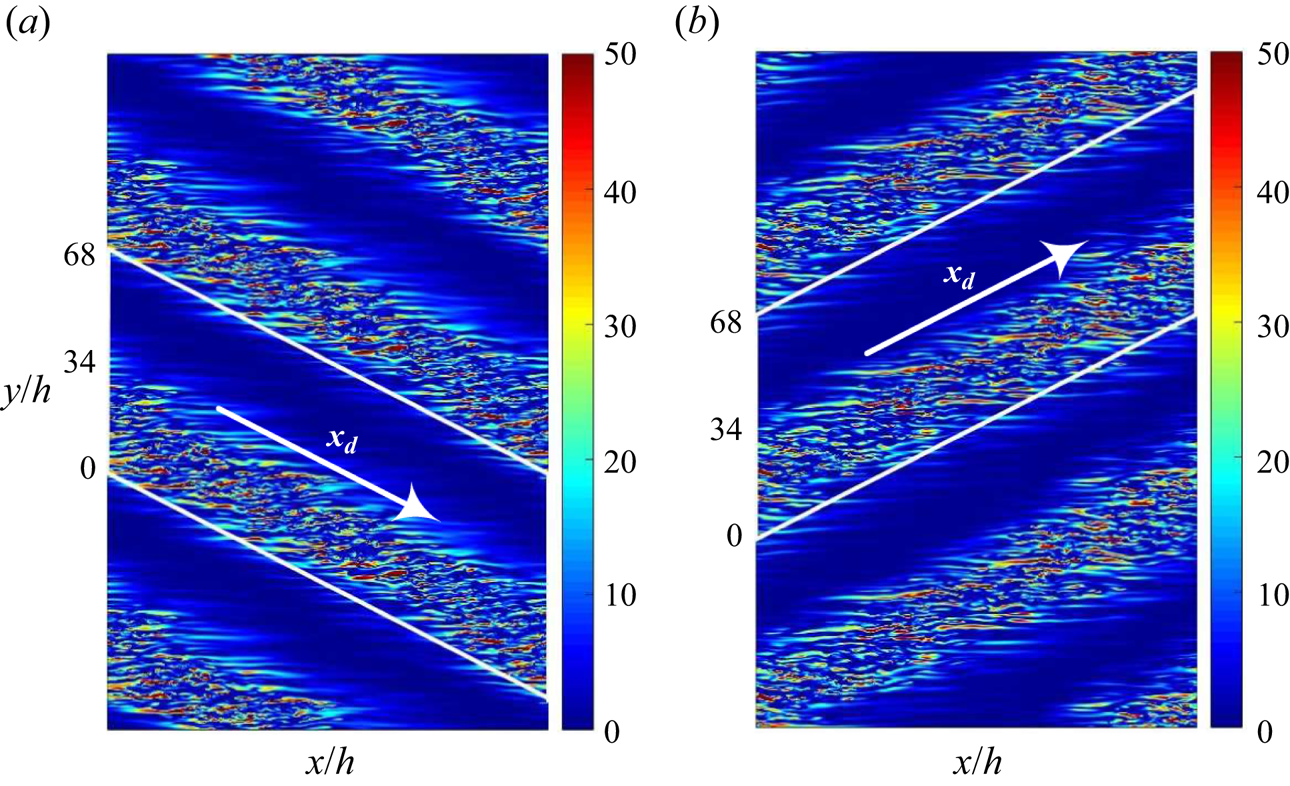
Figure 20. Contours of ![]() ${u}'{u}'$ at the midgap location (
${u}'{u}'$ at the midgap location (![]() $z=h$) for (a) d-type roughness (
$z=h$) for (a) d-type roughness (![]() $Re=350$) and (b) k-type roughness (
$Re=350$) and (b) k-type roughness (![]() $Re=300$). The product of streamwise velocity fluctuations is normalised by
$Re=300$). The product of streamwise velocity fluctuations is normalised by ![]() $u_{\tau }^{2}$ of each case.
$u_{\tau }^{2}$ of each case.

Figure 21. Diagonally averaged ![]() $\langle {u}'{u}'\rangle _{d}$ in the
$\langle {u}'{u}'\rangle _{d}$ in the ![]() $y$–
$y$–![]() $z$ plane for (a) d-type roughness (
$z$ plane for (a) d-type roughness (![]() $Re=350$) and (b) k-type roughness (
$Re=350$) and (b) k-type roughness (![]() $Re=300$). The data are normalised by
$Re=300$). The data are normalised by ![]() $u_{\tau }^{2}$ of each case. Note that
$u_{\tau }^{2}$ of each case. Note that ![]() $\langle \ \rangle _{d}$ represents spatial averaging along the bands (diagonal).
$\langle \ \rangle _{d}$ represents spatial averaging along the bands (diagonal).
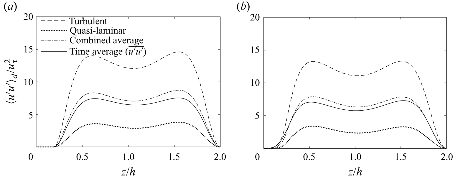
Figure 22. Wall-normal variation of ![]() $\langle {u}'{u}'\rangle _{d}$ for (a) d-type roughness (
$\langle {u}'{u}'\rangle _{d}$ for (a) d-type roughness (![]() $Re=350$) and (b) k-type roughness (
$Re=350$) and (b) k-type roughness (![]() $Re=300$). The variation of Reynolds stress
$Re=300$). The variation of Reynolds stress ![]() $\overline {u^{\prime }u^{\prime }}$ (obtained using time averaging) at the midcavity (
$\overline {u^{\prime }u^{\prime }}$ (obtained using time averaging) at the midcavity (![]() ${\rm I}$) location is also presented for comparison. Profiles are normalised by
${\rm I}$) location is also presented for comparison. Profiles are normalised by ![]() $u_{\tau }^{2}$ of each case.
$u_{\tau }^{2}$ of each case.
4. Conclusions
DNS have been performed to study the effect of roughness on the transition to turbulence in pCf. Two rough pCf cases are considered, with pitch separations ![]() $\lambda =2k$ and
$\lambda =2k$ and ![]() $\lambda =10k$, which fall in the d-type and the k-type roughness category, respectively. Reynolds number is reduced gradually in steps to achieve a reverse transition. Smooth pCf is known to have stable laminar–turbulent bands for
$\lambda =10k$, which fall in the d-type and the k-type roughness category, respectively. Reynolds number is reduced gradually in steps to achieve a reverse transition. Smooth pCf is known to have stable laminar–turbulent bands for ![]() $Re \in [325,400]$. Similar to the smooth pCf, a stage of oblique laminar–turbulent bands is found in both the d-type and the k-type roughness in the transitional regime. In the k-type roughness, stable laminar–turbulent bands are observed for the Reynolds numbers in the range
$Re \in [325,400]$. Similar to the smooth pCf, a stage of oblique laminar–turbulent bands is found in both the d-type and the k-type roughness in the transitional regime. In the k-type roughness, stable laminar–turbulent bands are observed for the Reynolds numbers in the range ![]() $Re \in [300, 325]$. The transitional range has narrowed and has shifted to lower Reynolds numbers compared with the smooth pCf. The ribs of the k-type roughness can act as vortex generators and aid the regeneration of vorticity so that the oblique bands are sustained at lower Reynolds numbers as opposed to the smooth pCf. However, the transitional range in the d-type roughness (
$Re \in [300, 325]$. The transitional range has narrowed and has shifted to lower Reynolds numbers compared with the smooth pCf. The ribs of the k-type roughness can act as vortex generators and aid the regeneration of vorticity so that the oblique bands are sustained at lower Reynolds numbers as opposed to the smooth pCf. However, the transitional range in the d-type roughness (![]() $Re \in [350,425]$) has shifted upwards compared with the smooth pCf. This peculiar behaviour is most likely due to the inherent lack of ability of the d-type roughness to effectively shed vortices into the outer flow and, thus, its negligible contribution to vorticity regeneration. Moreover, the streamwise-elongated structures in the d-type roughness are located further away from the wall, indicating a relatively stable zone in the near-wall region that could potentially inhibit streak formation. Previous studies on d-type roughness with a pitch separation of
$Re \in [350,425]$) has shifted upwards compared with the smooth pCf. This peculiar behaviour is most likely due to the inherent lack of ability of the d-type roughness to effectively shed vortices into the outer flow and, thus, its negligible contribution to vorticity regeneration. Moreover, the streamwise-elongated structures in the d-type roughness are located further away from the wall, indicating a relatively stable zone in the near-wall region that could potentially inhibit streak formation. Previous studies on d-type roughness with a pitch separation of ![]() $\lambda = 2k$ (e.g. Leonardi et al. Reference Leonardi, Orlandi, Djenidi and Antonia2004, Reference Leonardi, Orlandi and Antonia2007; MacDonald et al. Reference MacDonald, Ooi, García-Mayoral, Hutchins and Chung2018) have not reported a significant difference in the near-wall streaks between the d-type roughness and the smooth case, except for a reduction in their length. However, these studies were conducted in channel flows at Reynolds numbers that are higher than those in the present study, which focuses on the characteristics of rough Couette flows within the transitional flow regime.
$\lambda = 2k$ (e.g. Leonardi et al. Reference Leonardi, Orlandi, Djenidi and Antonia2004, Reference Leonardi, Orlandi and Antonia2007; MacDonald et al. Reference MacDonald, Ooi, García-Mayoral, Hutchins and Chung2018) have not reported a significant difference in the near-wall streaks between the d-type roughness and the smooth case, except for a reduction in their length. However, these studies were conducted in channel flows at Reynolds numbers that are higher than those in the present study, which focuses on the characteristics of rough Couette flows within the transitional flow regime.
The large-scale flow in the rough pCf cases is parallel to the oblique bands near the laminar–turbulent boundaries, indicative of a significant spanwise velocity component. The peak of the probability density function of the angle made by the large-scale flow vectors gives the most likely orientation of the large-scale flow. As a major portion of the flow is parallel to the oblique bands, the most likely angle matches well with the corresponding pattern angle. Similar to the spatial planes, spatiotemporal diagrams reveal laminar–turbulent coexistence as oblique bands. The frequency/time period of the patterns in the rough pCf cases is found using an FFT technique. The pattern in the d-type roughness has about four cycles in ![]() $1000h/U_{w}$, and its k-type counterpart has approximately three cycles every
$1000h/U_{w}$, and its k-type counterpart has approximately three cycles every ![]() $1000h/U_{w}$. The frequency/time period remains the same regardless of the Reynolds number.
$1000h/U_{w}$. The frequency/time period remains the same regardless of the Reynolds number.
The secondary flow in the transitional regime shows the presence of counter-rotating vortices in the turbulent regions. These vortices are integral in maintaining the elongated streaks which constitute the turbulent bands. The main effect of having a non-zero spanwise velocity is reflected in the off-diagonal components of the Reynolds stress tensor. The gradient ![]() ${\partial \bar {v}}/{\partial z}$ in the production term of the Reynolds stresses
${\partial \bar {v}}/{\partial z}$ in the production term of the Reynolds stresses ![]() $-\overline {v^{\prime }u^{\prime }}$ and
$-\overline {v^{\prime }u^{\prime }}$ and ![]() $-\overline {w^{\prime }v^{\prime }}$ does not approach zero, leading to non-zero production.
$-\overline {w^{\prime }v^{\prime }}$ does not approach zero, leading to non-zero production. ![]() $-\overline {v^{\prime }u^{\prime }}$ and
$-\overline {v^{\prime }u^{\prime }}$ and ![]() $-\overline {w^{\prime }v^{\prime }}$, which were zero in the turbulent regime, are now non-zero and, thus, relevant.
$-\overline {w^{\prime }v^{\prime }}$, which were zero in the turbulent regime, are now non-zero and, thus, relevant.
The results from the present study can be compared with those of Ishida et al. (Reference Ishida, Brethouwer, Duguet and Tsukahara2017). Both studies concur that the transition to turbulence occurs through a stage of alternate laminar–turbulent bands when the roughness height is ![]() $k=0.2h$. Their model predicts a rise in the friction Reynolds number due to roughness, and this observation aligns with the behaviour of the k-type roughness employed in the present study. Apart from these points, a direct quantitative comparison is challenging as the present roughness pitch analogous to the roughness density used in their parametric model is difficult to determine. We anticipate that forthcoming research will further substantiate our findings. We also believe that this study provides a foundational understanding of the effects of roughness on the transition to turbulence in pCf. It can be extended to investigate the effect of roughness by altering the shape, height, dimensionality and arrangement of the roughness. Configurations such as longitudinal roughness, oblique roughness and incoherent random roughness can also be considered.
$k=0.2h$. Their model predicts a rise in the friction Reynolds number due to roughness, and this observation aligns with the behaviour of the k-type roughness employed in the present study. Apart from these points, a direct quantitative comparison is challenging as the present roughness pitch analogous to the roughness density used in their parametric model is difficult to determine. We anticipate that forthcoming research will further substantiate our findings. We also believe that this study provides a foundational understanding of the effects of roughness on the transition to turbulence in pCf. It can be extended to investigate the effect of roughness by altering the shape, height, dimensionality and arrangement of the roughness. Configurations such as longitudinal roughness, oblique roughness and incoherent random roughness can also be considered.
Funding
This work is financially supported by the Science and Engineering Research Board (SERB), Department of Science and Technology, Government of India (Core Research Grant No. CRG/2018/004926).
Declaration of interests
The authors report no conflict of interest.
Appendix A
A.1. Mean quantities at  $Re=500$
Figures 23 and 24 show the mean quantities at ![]() $Re=500$.
$Re=500$.
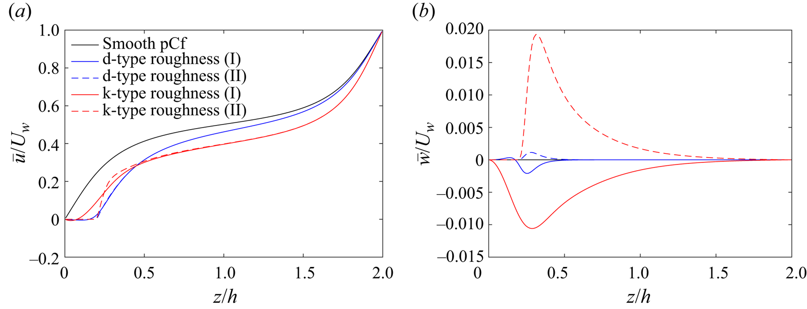
Figure 23. Variation of (a) mean streamwise velocity ![]() $\bar {u}$ and (b) mean wall-normal velocity
$\bar {u}$ and (b) mean wall-normal velocity ![]() $\bar {w}$ along the wall-normal direction for d-type roughness and k-type roughness at the midcavity (I) and midrib (II) locations at
$\bar {w}$ along the wall-normal direction for d-type roughness and k-type roughness at the midcavity (I) and midrib (II) locations at ![]() $Re = 500$. Velocity profiles in smooth pCf (
$Re = 500$. Velocity profiles in smooth pCf (![]() $Re = 500$) is also plotted for comparison. Mean spanwise velocity
$Re = 500$) is also plotted for comparison. Mean spanwise velocity ![]() $\bar {v}$ is negligible for all the cases.
$\bar {v}$ is negligible for all the cases.
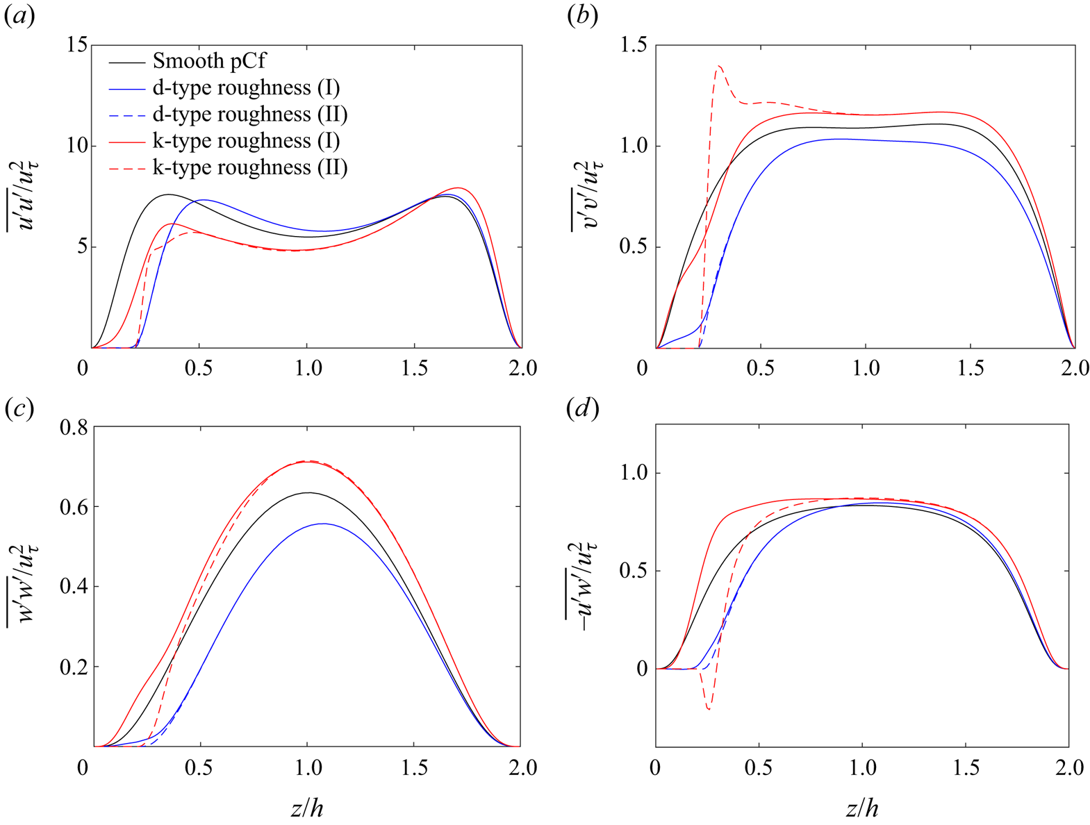
Figure 24. Variation of components of Reynolds stress tensor along the wall-normal direction for d-type roughness and k-type roughness at the midcavity (I) and midrib (II) locations at ![]() $Re = 500$. Reynolds stresses in smooth pCf (
$Re = 500$. Reynolds stresses in smooth pCf (![]() $Re = 500$) are also plotted for comparison. Here
$Re = 500$) are also plotted for comparison. Here ![]() $-\overline {v^{\prime }u^{\prime }}$ and
$-\overline {v^{\prime }u^{\prime }}$ and ![]() $-\overline {w^{\prime }v^{\prime }}$ are negligible for all the cases. The stresses are normalised using the square of global friction velocity
$-\overline {w^{\prime }v^{\prime }}$ are negligible for all the cases. The stresses are normalised using the square of global friction velocity ![]() $u_{\tau }^{2}$ of each case.
$u_{\tau }^{2}$ of each case.
A.2. Apparent midgap
The apparent midgap is located at the minimum of ![]() ${{\rm d}\bar {u}}/{{\rm d} z}$ above the roughness layer (Ishida et al. Reference Ishida, Brethouwer, Duguet and Tsukahara2017). The apparent midgaps and the corresponding mean streamwise velocities for the rough pCf cases are marked in figure 25.
${{\rm d}\bar {u}}/{{\rm d} z}$ above the roughness layer (Ishida et al. Reference Ishida, Brethouwer, Duguet and Tsukahara2017). The apparent midgaps and the corresponding mean streamwise velocities for the rough pCf cases are marked in figure 25.

Figure 25. Variation of (a) mean velocity gradient ![]() ${{\rm d} \bar {u}}/{{\rm d} z}$ and (b) mean streamwise velocity
${{\rm d} \bar {u}}/{{\rm d} z}$ and (b) mean streamwise velocity ![]() $\bar {u}$ along the wall-normal direction for d-type roughness and k-type roughness at the midcavity (I) and midrib (II) locations at a Reynolds number close to their
$\bar {u}$ along the wall-normal direction for d-type roughness and k-type roughness at the midcavity (I) and midrib (II) locations at a Reynolds number close to their ![]() $Re_{g}$. Corresponding profiles in smooth pCf are also plotted for comparison.
$Re_{g}$. Corresponding profiles in smooth pCf are also plotted for comparison.
A.3. Turbulent and quasi-laminar components of  $\langle {u}'_{i}{u}'_{j}\rangle _{d}$
The turbulent and quasi-laminar components of ![]() $\langle {u}'_{i}{u}'_{j}\rangle _{d}$ are plotted in figure 26.
$\langle {u}'_{i}{u}'_{j}\rangle _{d}$ are plotted in figure 26.
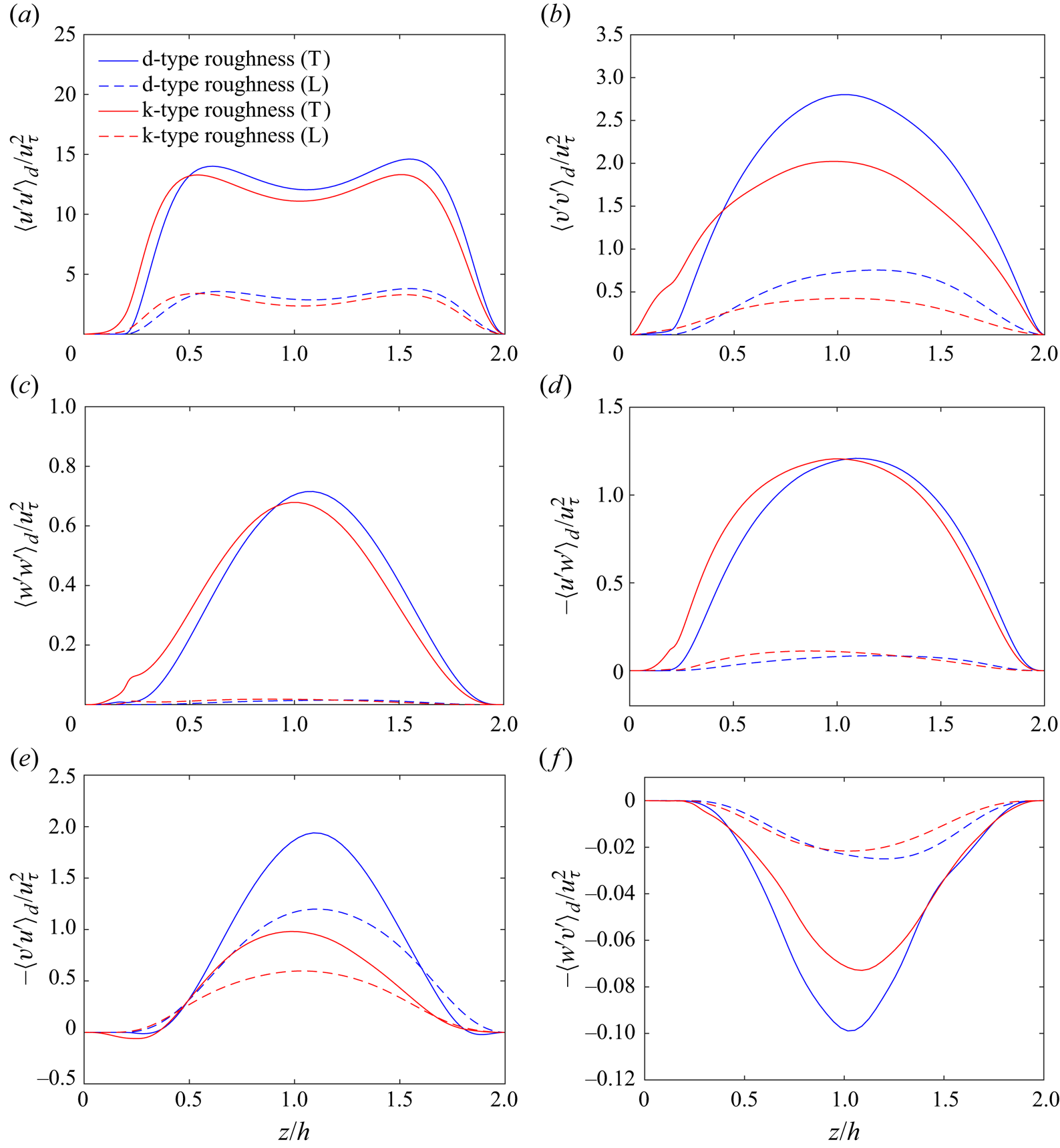
Figure 26. Wall-normal variation of ![]() $\langle {u}'_{i}{u}'_{j}\rangle _{d}$ for the rough pCf cases at a Reynolds number close to their
$\langle {u}'_{i}{u}'_{j}\rangle _{d}$ for the rough pCf cases at a Reynolds number close to their ![]() $Re_{g}$. The values are normalised using
$Re_{g}$. The values are normalised using ![]() $u_{\tau }^{2}$ of each case. The legend labels (T) and (L) indicate the turbulent and quasi-laminar regions, respectively.
$u_{\tau }^{2}$ of each case. The legend labels (T) and (L) indicate the turbulent and quasi-laminar regions, respectively.

