

1 Introduction
The zeta-regularized determinant of the Laplacian, introduced in [Reference Ray and Singer14], is a global spectral invariant of smooth Riemannian manifolds with important interpretations and applications in geometry, topology, and mathematical physics (see Chapter 5 of [Reference Rosenberg15] for an overview and [Reference Osgood, Phillips and Sarnak13] for an elegant application). Explicitly computing this invariant is typically impossible, but a useful tool to understand its nature is the Mayer–Vietoris type gluing formula proven by Burghelea, Friedlander, and Kappeler in [Reference Burghelea, Friedlander and Kappeler3], commonly called the BFK formula. The BFK formula, which applies to a broad class of elliptic boundary problems on bundles, relates the determinant of an elliptic differential operator across different complementary boundary conditions via the determinant of an intermediate lower-order pseudodifferential operator on the boundary.
This formula is part of a broader body of work which seeks to understand how various global spectral quantities localize on manifolds. Such results have been successfully proved through various approaches; we provide several examples chronologically for context. In [Reference Burghelea, Friedlander and Kappeler3], where the original proof of the BFK formula is presented, the authors perturb the interior operator by adding to it a multiple of the identity, then explicitly compute the corresponding variation of the determinant in terms of the perturbation parameter. In [Reference Müller12], Müller studies how the eta invariant, another natural spectral quantity which arises in index theory, varies on a manifold with cylindrical boundary as the boundary gets pushed to infinity. In [Reference Mazzeo and Melrose11], Mazzeo and Melrose compute how the eta invariant varies under analytic surgery, in which a submanifold is pushed to infinity by taking degenerating metrics which limit to a b-metric. These ideas are extended by Hassell, Mazzeo, and Melrose in [Reference Hassell, Mazzeo and Melrose6], and applied to handle analytic torsion, a spectral invariant with connections to the combinatorial structure of the underlying manifold. In [Reference Bunke2], Bunke studies the adiabatic limit of the eta invariant of the Dirac operator associated with a pair of APS-type boundary conditions. In [Reference Cappell, Lee and Miller4], Cappell, Lee, and Miller develop a splicing technique which is applied to study localization of low eigensolutions of a self-adjoint elliptic operator. And in [Reference Brüning and Lesch1], Brüning and Lesch study the Dirac operator on a manifold with boundary, continuously deform the domain of the operator by varying the boundary conditions, and compute how the eta invariant of the Dirac operator changes through this deformation.
In this article, we present a new proof of the BFK formula, inspired mainly by the arguments in [Reference Brüning and Lesch1]. We develop this deformation approach with the aim of obtaining a proof method which will more readily generalize to settings where we cut along submanifolds with geometric singularities such as corners. For clarity, we state the main result here but delay precise definitions to the next section.
Let A be an admissible elliptic differential operator of positive order on a compact manifold M with nonempty boundary N. Fix $B_0$
and
$B_0$
and $B_1$
two complementary boundary conditions, and take Q to be the induced correspondence operator on the boundary. Then, with
$B_1$
two complementary boundary conditions, and take Q to be the induced correspondence operator on the boundary. Then, with $A_i$
denoting the operator A confined to the domain
$A_i$
denoting the operator A confined to the domain $\ker B_i$
, we have the following theorem.
$\ker B_i$
, we have the following theorem.
Theorem 1.1 (The BFK Formula [Reference Burghelea, Friedlander and Kappeler3])
The zeta-regularized determinants of $A_0$
and
$A_0$
and $A_1$
are related by
$A_1$
are related by
 $$ \begin{align} \frac{\det A_1}{\det A_0}=c\cdot \det Q, \end{align} $$
where c is a local quantity which can be computed in terms of the symbols of A, $B_0$
, and
$B_0$
, and $B_1$
along N.
$B_1$
along N.
The proof of Theorem 1.1 presented here proceeds by explicitly considering how the determinant varies along a family of operators $A_t$
interpolating between
$A_t$
interpolating between $A_0$
and
$A_0$
and $A_1$
, rather than by perturbing the interior operator directly, as originally done in [Reference Burghelea, Friedlander and Kappeler3].
$A_1$
, rather than by perturbing the interior operator directly, as originally done in [Reference Burghelea, Friedlander and Kappeler3].
Remark 1.2 To provide context to this approach, we describe here in more detail the strategy employed by Brüning and Lesch in [Reference Brüning and Lesch1]. The authors obtain a gluing law for the eta invariant associated with a Dirac operator on a manifold with boundary by rotating through a family of boundary conditions. More specifically, they consider a Hermitian vector bundle E over a compact Riemannian manifold M, and a first-order symmetric elliptic differential operator D acting on smooth sections of the bundle (the main example of which are Dirac operators). With $N\subset M$
a compact hypersurface, they note that D restricted to
$N\subset M$
a compact hypersurface, they note that D restricted to $C^\infty (E|_{M\setminus N})$
is no longer essentially self-adjoint, and consider therefore two natural boundary conditions: the APS boundary condition and the continuous transmission boundary condition. The authors then explicitly parametrize a path between these boundary conditions and show that the variation of the eta invariant across this path can be computed by studying the operator D, conjugated by appropriate rotations which map between the domains corresponding to each of the boundary conditions. (Details are outlined in Section 3 of [Reference Brüning and Lesch1].)
$C^\infty (E|_{M\setminus N})$
is no longer essentially self-adjoint, and consider therefore two natural boundary conditions: the APS boundary condition and the continuous transmission boundary condition. The authors then explicitly parametrize a path between these boundary conditions and show that the variation of the eta invariant across this path can be computed by studying the operator D, conjugated by appropriate rotations which map between the domains corresponding to each of the boundary conditions. (Details are outlined in Section 3 of [Reference Brüning and Lesch1].)
Our proof carries this idea over to the zeta-regularized determinant. The main difference is that there is no longer a natural set of rotations carrying the domain corresponding to one boundary condition to that corresponding to the other boundary condition. Instead, we work directly with the resolvent, and obtain variational formulas by studying how this operator changes as we interpolate between $B_0$
and
$B_0$
and $B_1$
.
$B_1$
.
In Section 2, we provide rigorous definitions and assumptions for our theorem, and place the BFK formula in context by describing as an example the case of the Laplacian on a compact Riemannian manifold. In Section 3, we prove several relationships linking the Poisson extension operator P, the operator Q which serves as an analog of the Dirichlet-to-Neumann map, and the resolvent R. In particular, we establish in Proposition 3.3 a surprising integral identity which later serves as the key for our proof. Finally, in Section 4, we use properties of the trace functional and identities from the meromorphic functional calculus to deduce a link between the zeta functions of $A_0, A_1$
and the trace of the operator Q. The main technical challenges arise here in the subtlety of trace class operators, and this is handled by introducing high powers of regularizing operators and then applying unique continuation to deduce results globally. Finally, we use these identities to deduce the BFK formula.
$A_0, A_1$
and the trace of the operator Q. The main technical challenges arise here in the subtlety of trace class operators, and this is handled by introducing high powers of regularizing operators and then applying unique continuation to deduce results globally. Finally, we use these identities to deduce the BFK formula.
2 Setup
We now describe in detail our setting, which is analogous to that of [Reference Burghelea, Friedlander and Kappeler3]. Let M be a compact manifold of dimension $d\geq 2$
with nonempty boundary
$d\geq 2$
with nonempty boundary $N=\partial M$
, and take
$N=\partial M$
, and take $E\to M$
to be a smooth vector bundle over M. Suppose
$E\to M$
to be a smooth vector bundle over M. Suppose $A\colon C^\infty (E)\to C^\infty (E)$
is an elliptic differential operator of order
$A\colon C^\infty (E)\to C^\infty (E)$
is an elliptic differential operator of order $\omega>0$
. Let
$\omega>0$
. Let $F_j\to N$
,
$F_j\to N$
, $1\leq j\leq k$
, be smooth vector bundles over the boundary, and consider for each j a pair of boundary differential operators
$1\leq j\leq k$
, be smooth vector bundles over the boundary, and consider for each j a pair of boundary differential operators $B^j_i \colon C^\infty (E)\to C^\infty (F_j)$
, for
$B^j_i \colon C^\infty (E)\to C^\infty (F_j)$
, for $i=0,1$
, such that
$i=0,1$
, such that $\text {ord}\,B_1^j-\text {ord}\,B_0^j$
is positive and constant in j, and
$\text {ord}\,B_1^j-\text {ord}\,B_0^j$
is positive and constant in j, and $\text {ord}\,B^j_i< \omega $
. Writing
$\text {ord}\,B^j_i< \omega $
. Writing
 $$ \begin{align} B_t^j=(1-t)B_0^j+tB_1^j\quad \text{and} \quad B_t=(B_t^1,\dots, B_t^k), \end{align} $$
we require that $B_0$
and
$B_0$
and $B_1$
be complementary, meaning that the intersection of their null spaces consists of sections of
$B_1$
be complementary, meaning that the intersection of their null spaces consists of sections of $C^\infty (E)$
which vanish up to order
$C^\infty (E)$
which vanish up to order $\omega -1$
on N.
$\omega -1$
on N.
Next, we assume that $(A,B_t)$
is an invertible elliptic boundary problem in the sense of [Reference Hörmander7] for
$(A,B_t)$
is an invertible elliptic boundary problem in the sense of [Reference Hörmander7] for $0\leq t\leq 1$
and hence extends to a bijective continuous operator
$0\leq t\leq 1$
and hence extends to a bijective continuous operator
 $$ \begin{align} (A,B_t)\colon H^\omega(E)\to L^2(E)\oplus H^{\omega-\omega_1(t)-1/2}(F_1)\oplus\dots \oplus H^{\omega-\omega_k(t)-1/2}(F_k), \end{align} $$
where $\omega _j(t)=\text {ord }B_t^j$
. Importantly, note that
$\omega _j(t)=\text {ord }B_t^j$
. Importantly, note that $\omega _j(t)$
is discontinuous at
$\omega _j(t)$
is discontinuous at $t=0$
.
$t=0$
.
Example 2.1 (The Laplacian on a manifold with boundary)
The following setup is our main motivating example. Suppose M is equipped with a Riemannian metric g and denote by $\Delta _g$
the corresponding (positive) Laplacian acting on
$\Delta _g$
the corresponding (positive) Laplacian acting on $C^\infty (M)$
. Define the Dirichlet and Neumann boundary operators, denoted
$C^\infty (M)$
. Define the Dirichlet and Neumann boundary operators, denoted $\mathcal {D}$
and
$\mathcal {D}$
and $\mathcal {N,}$
respectively, by
$\mathcal {N,}$
respectively, by
 $$ \begin{align} \mathcal{D}u=u|_{\partial M} \quad \text{and}\quad \mathcal{N}u=\frac{\partial u}{\partial n}\Big{|}_{\partial M}, \end{align} $$
where n is the outward-pointing unit normal at the boundary. With E and $F_1$
the trivial line bundles over their respective spaces (i.e., considering the Laplacian acting simply on real-valued functions), set
$F_1$
the trivial line bundles over their respective spaces (i.e., considering the Laplacian acting simply on real-valued functions), set $B_0=\mathcal {D}$
and
$B_0=\mathcal {D}$
and $B_1=\mathcal {N}$
. Finally, to ensure invertibility, set
$B_1=\mathcal {N}$
. Finally, to ensure invertibility, set $A=\Delta _g+\epsilon $
for some positive
$A=\Delta _g+\epsilon $
for some positive $\epsilon $
. The discussed assumptions are then clearly satisfied.
$\epsilon $
. The discussed assumptions are then clearly satisfied.
Let $A_t$
denote the operator which acts as A on its domain
$A_t$
denote the operator which acts as A on its domain $\text {dom}(A_t)=\ker (B_t)\subset H^\omega (E)$
, and define the corresponding resolvent operator by
$\text {dom}(A_t)=\ker (B_t)\subset H^\omega (E)$
, and define the corresponding resolvent operator by
 $$ \begin{align}\begin{aligned} R_t(z)\colon L^2(E)&\to H^\omega(E)\\ u&\mapsto(A-z,B_t)^{-1}(u,0) \end{aligned}\end{align} $$
and Poisson operator by
 $$ \begin{align}\begin{aligned} P_t(z)\colon H^{\omega-\omega_1(t)-1/2}(F_1)\oplus\dots \oplus H^{\omega-\omega_k(t)-1/2}(F_k)&\to H^\omega(E)\\ f=(f_1,\dots, f_k) & \mapsto (A-z,B_t)^{-1}(0,f). \end{aligned}\end{align} $$
Both of these families of operators depend meromorphically on z as a consequence of the analytic Fredholm theorem.
Away from the spectrum of $A_0$
, the triple
$A_0$
, the triple $(A-z, B_0, B_1)$
gives rise to a natural map between sections of
$(A-z, B_0, B_1)$
gives rise to a natural map between sections of $\oplus _jF_j$
which correspond to each other as the image under either
$\oplus _jF_j$
which correspond to each other as the image under either $B_0$
or
$B_0$
or $B_1$
of a solution of
$B_1$
of a solution of $(A-z)u=0$
. This map is given by the operator
$(A-z)u=0$
. This map is given by the operator $Q(z)=B_1P_0(z)$
, which we assume to be positive and self-adjoint when z is in the ray
$Q(z)=B_1P_0(z)$
, which we assume to be positive and self-adjoint when z is in the ray $\mathbb {R}_-=\{r e^{i\pi } r \geq 0\}$
. We shall write
$\mathbb {R}_-=\{r e^{i\pi } r \geq 0\}$
. We shall write $Q=Q(0)$
.
$Q=Q(0)$
.
Example 2.2 (The Dirichlet-to-Neumann map)
We continue with Example 2.1. In that setting, the problem $(A=\Delta _g+\epsilon , B_t=(1-t)\mathcal {D}+t\mathcal {N})$
is well known to be an elliptic boundary problem (see [Reference Hörmander7] for an extensive discussion, for example). The operator
$(A=\Delta _g+\epsilon , B_t=(1-t)\mathcal {D}+t\mathcal {N})$
is well known to be an elliptic boundary problem (see [Reference Hörmander7] for an extensive discussion, for example). The operator $Q(z)$
described above corresponds to the standard Dirichlet-to-Neumann map on N with respect to interior extension operator
$Q(z)$
described above corresponds to the standard Dirichlet-to-Neumann map on N with respect to interior extension operator $\Delta _g+\epsilon -z$
. In this setting, it is clear to see why the restriction
$\Delta _g+\epsilon -z$
. In this setting, it is clear to see why the restriction $z\notin \text {spec }A_0$
is necessary:
$z\notin \text {spec }A_0$
is necessary: $P_0(z)$
fails to be well defined precisely when the problem
$P_0(z)$
fails to be well defined precisely when the problem $(\Delta _g+\epsilon -z)u=0$
on M,
$(\Delta _g+\epsilon -z)u=0$
on M, $u=f$
on N does not have a unique solution. Indeed, if
$u=f$
on N does not have a unique solution. Indeed, if $u,\tilde u$
are two distinct solutions to the problem, observe
$u,\tilde u$
are two distinct solutions to the problem, observe $u-\tilde u$
is a z-eigenfunction of
$u-\tilde u$
is a z-eigenfunction of $A_0$
(and, in the other direction, the existence of such an eigenfunction obstructs uniqueness of extensions). Next, we confirm that
$A_0$
(and, in the other direction, the existence of such an eigenfunction obstructs uniqueness of extensions). Next, we confirm that $Q(z)$
is positive and self-adjoint on
$Q(z)$
is positive and self-adjoint on $\mathbb {R}_-$
: by Green’s identity,
$\mathbb {R}_-$
: by Green’s identity,
since $z<0$
, and similarly
$z<0$
, and similarly
 $$ \begin{align}\begin{aligned} \left\langle f,Q(z)g \right\rangle_{L^2(N)}-\left\langle Q(z)f,g \right\rangle_{L^2(N)}&=\left\langle B_0P_0(z)f,B_1P_0(z)g \right\rangle_{L^2(N)}\\ &\qquad -\left\langle B_1P_0(z)f,B_0P_0(z)g \right\rangle_{L^2(N)}\\ &= (z-\overline z)\left\langle P_0(z)f,P_0(z)g \right\rangle_{L^2(M)}, \end{aligned}\end{align} $$
which vanishes when $z\in \mathbb {R}$
.
$z\in \mathbb {R}$
.
Remark 2.3 Note that the computations presented above hold more generally when A is a symmetric divergence-form elliptic operator, thus the assumption that $Q(z)$
is self-adjoint on
$Q(z)$
is self-adjoint on $\mathbb {R}_-$
is automatically satisfied in those cases. In general, however, this assumption will be necessary for Proposition 3.3 to hold.
$\mathbb {R}_-$
is automatically satisfied in those cases. In general, however, this assumption will be necessary for Proposition 3.3 to hold.
In order to ensure that our operators have well-defined zeta-regularized determinants, we shall require that they satisfy additional spectral properties which guarantee certain path integrals in $\mathbb {C}$
to be well defined and convergent. This is captured by the following definition.
$\mathbb {C}$
to be well defined and convergent. This is captured by the following definition.
Definition 2.1 For B any boundary differential operator such that $(A,B)$
is an elliptic boundary problem, the angle
$(A,B)$
is an elliptic boundary problem, the angle $\theta $
is a principal angle for
$\theta $
is a principal angle for $(A,B)$
if the following conditions are satisfied:
$(A,B)$
if the following conditions are satisfied:
-
(1) (Agmon angle condition) For every $p\in M$
and
$\xi \in T^*_p(M)\setminus 0$
, we have (2.8)where
$$ \begin{align} \text{spec } \sigma_\omega(A)(p,\xi)\cap \{r e^{i\theta} r \geq 0\}=\varnothing, \end{align} $$
$\sigma _\omega (A)$
denotes the principal symbol of A.
$p\in M$
and
$\xi \in T^*_p(M)\setminus 0$
, we have (2.8)where
$$ \begin{align} \text{spec } \sigma_\omega(A)(p,\xi)\cap \{r e^{i\theta} r \geq 0\}=\varnothing, \end{align} $$
$\sigma _\omega (A)$
denotes the principal symbol of A.
-
(2) (Shapiro–Lopatinski condition) In a collar neighborhood
$N\times [0,\infty )$
of the boundary, let
$(x,y)$
denote the induced coordinates and
$(\eta ,\tau )$
the corresponding coordinates on the cotangent bundle. Write
$\alpha =(\alpha ',\alpha _d)$
, a multi-index of length d, and say
$A=\sum _{\alpha }a_\alpha (p)D^\alpha $
in coordinates. Then, given
$r\geq 0$
and
$f_j\in F_j$
for
$1\leq j\leq k$
, there exists a unique solution
$u(x,y)$
to (2.9)satisfying both
$\lim _{y\to \infty }u(x,y)=0$
and (2.10)for every j.
$$ \begin{align} \sum_{l=\omega-\omega_j}^\omega \sigma_{\omega_j}(B_j)(x,\eta)D_y^{\omega-l}u(x,0)=f_j \end{align} $$


We assume that $\pi $
is a principal angle for
$\pi $
is a principal angle for $(A,B_t)$
for every
$(A,B_t)$
for every $0\leq t\leq 1$
, which allows us to define complex powers of
$0\leq t\leq 1$
, which allows us to define complex powers of $A_t$
as in the Seeley calculus. To this end, let
$A_t$
as in the Seeley calculus. To this end, let
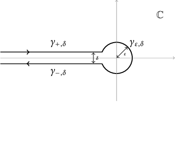
 $\gamma $
be a contour in the complex plane around the ray
$\gamma $
be a contour in the complex plane around the ray $\mathbb {R}_-$
traveling clockwise around the origin, so that it positively winds around every point of the spectrum (see Figure 1). Taking the branch cut of
$\mathbb {R}_-$
traveling clockwise around the origin, so that it positively winds around every point of the spectrum (see Figure 1). Taking the branch cut of $z^{-s}$
along
$z^{-s}$
along $\mathbb {R}_-$
, define
$\mathbb {R}_-$
, define
 $$ \begin{align} A_t^{-s}=\frac{i}{2\pi}\int_{\gamma} z^{-s}R_t(z)\, d z. \end{align} $$
When $\text {Re}(s)$
is sufficiently large, this operator is well defined and trace class. Its trace, denoted by
$\text {Re}(s)$
is sufficiently large, this operator is well defined and trace class. Its trace, denoted by $\zeta _t(s)$
, extends meromorphically to the whole complex plane and is regular at
$\zeta _t(s)$
, extends meromorphically to the whole complex plane and is regular at $s=0$
(we refer the reader to [Reference Seeley18, Reference Seeley19] for details). Finally, we may now define
$s=0$
(we refer the reader to [Reference Seeley18, Reference Seeley19] for details). Finally, we may now define
 $$ \begin{align} \det A_t=e^{-\zeta_t'(0)}, \end{align} $$
the zeta-regularized determinant of $A_t$
.
$A_t$
.

Figure 1 The contour $\gamma $
used in the proof of Theorem 1.1.
$\gamma $
used in the proof of Theorem 1.1.
Example 2.4 (The determinant of the Laplacian)
We continue with Examples 2.1 and 2.2. Since $A_t$
, which is simply
$A_t$
, which is simply $\Delta _g+\epsilon $
restricted to the Robin-boundary condition domain
$\Delta _g+\epsilon $
restricted to the Robin-boundary condition domain $\ker ((1-t)\mathcal {D}+t\mathcal {N}))$
, is a positive self-adjoint operator and its principal symbol is
$\ker ((1-t)\mathcal {D}+t\mathcal {N}))$
, is a positive self-adjoint operator and its principal symbol is ![]() , conditions 1 and 2 in the definition of principal angle are satisfied with
, conditions 1 and 2 in the definition of principal angle are satisfied with $\theta =\pi $
. We may then define
$\theta =\pi $
. We may then define $A_t^{-s}$
, and the Weyl law tells us that this will be a bounded (and in fact trace class) operator when
$A_t^{-s}$
, and the Weyl law tells us that this will be a bounded (and in fact trace class) operator when $\text {Re}(s)>d/2$
. In fact, denoting the eigenvalues of
$\text {Re}(s)>d/2$
. In fact, denoting the eigenvalues of $A_t$
by
$A_t$
by $\lambda _1,\lambda _2,\dots $
, we may rewrite
$\lambda _1,\lambda _2,\dots $
, we may rewrite
 $$ \begin{align} \text{Tr}(A_t^{-s})=\sum_j \lambda_j^{-s} \end{align} $$
to then note the connection to the standard zeta function. We may then seek to take $\epsilon \to 0$
and regularize the limit in order to get a well-defined determinant of the genuine Laplacian, rather than its shift A. This works, and is described in the proof of Theorem B* in [Reference Burghelea, Friedlander and Kappeler3]. See also [Reference Lee9] for further specialization to Laplace-type operators.
$\epsilon \to 0$
and regularize the limit in order to get a well-defined determinant of the genuine Laplacian, rather than its shift A. This works, and is described in the proof of Theorem B* in [Reference Burghelea, Friedlander and Kappeler3]. See also [Reference Lee9] for further specialization to Laplace-type operators.
Next, we seek to extend our definition of zeta-regularized determinant to matrices of operators since $Q(z)$
, which appears in the right-hand side of Equation (1.1), is a
$Q(z)$
, which appears in the right-hand side of Equation (1.1), is a $k\times k$
matrix of
$k\times k$
matrix of $\Psi $
DOs. The necessary properties are described in the following definition.
$\Psi $
DOs. The necessary properties are described in the following definition.
Definition 2.2 We say the operator $Q=\left ( Q_{ij} \right )\colon \oplus _{j=1}^k C^\infty (F_j)\to \oplus _{j=1}^k C^\infty (F_j)$
is of order
$Q=\left ( Q_{ij} \right )\colon \oplus _{j=1}^k C^\infty (F_j)\to \oplus _{j=1}^k C^\infty (F_j)$
is of order $(\alpha _1,\dots , \alpha _k;\beta _1,\dots , \beta _k)$
if
$(\alpha _1,\dots , \alpha _k;\beta _1,\dots , \beta _k)$
if $\text {ord }Q_{ij}=\alpha _i+\beta _j$
. Define then the principal symbol of Q to be the matrix
$\text {ord }Q_{ij}=\alpha _i+\beta _j$
. Define then the principal symbol of Q to be the matrix $\sigma (Q)=\left ( \sigma _{\alpha _i+\beta _j}(Q_{ij}) \right )$
, and say Q is elliptic in the sense of Agmon, Douglis, and Nirenberg if for any
$\sigma (Q)=\left ( \sigma _{\alpha _i+\beta _j}(Q_{ij}) \right )$
, and say Q is elliptic in the sense of Agmon, Douglis, and Nirenberg if for any $p\in M$
and
$p\in M$
and $\xi \in T^*_p(M)\setminus 0$
, the map
$\xi \in T^*_p(M)\setminus 0$
, the map $\sigma (Q)(p,\xi )$
is invertible.
$\sigma (Q)(p,\xi )$
is invertible.
We shall show in Proposition 3.2 that $Q(z)$
is indeed elliptic in the sense of Agmon, Douglis, and Nirenberg when
$Q(z)$
is indeed elliptic in the sense of Agmon, Douglis, and Nirenberg when $z\notin \text {spec }A_0$
. With minor modification, the notion of a principal angle carries over to such operators, and we assume that
$z\notin \text {spec }A_0$
. With minor modification, the notion of a principal angle carries over to such operators, and we assume that $\pi $
is also a principal angle for
$\pi $
is also a principal angle for $Q(z)$
, hence, the determinant of
$Q(z)$
, hence, the determinant of $Q(z)$
is well defined (again only when
$Q(z)$
is well defined (again only when $z\notin \text {spec }A_0$
). The details of these definitions can be found in Section 2 of [Reference Burghelea, Friedlander and Kappeler3].
$z\notin \text {spec }A_0$
). The details of these definitions can be found in Section 2 of [Reference Burghelea, Friedlander and Kappeler3].
Remark 2.5 For simplicity, we have taken $\pi $
to be the principal angle for all involved operators. In particular, this is the case for the discussed example of the Laplacian on a manifold, as the Dirichlet-to-Neumann operator is positive. However, all proofs presented below can be modified to the general case without too much complication: one must ensure that the path
$\pi $
to be the principal angle for all involved operators. In particular, this is the case for the discussed example of the Laplacian on a manifold, as the Dirichlet-to-Neumann operator is positive. However, all proofs presented below can be modified to the general case without too much complication: one must ensure that the path $\gamma $
used in the Seeley calculus is adapted to the principal angle, and that the dependence of the determinants on the principal angle be made explicit. The proof in [Reference Burghelea, Friedlander and Kappeler3], for example, accounts for these details. Our proof, however, has an additional assumption: we make use of the fact that
$\gamma $
used in the Seeley calculus is adapted to the principal angle, and that the dependence of the determinants on the principal angle be made explicit. The proof in [Reference Burghelea, Friedlander and Kappeler3], for example, accounts for these details. Our proof, however, has an additional assumption: we make use of the fact that $Q(z)$
is self-adjoint when
$Q(z)$
is self-adjoint when $z\in \mathbb {R}_-$
in Proposition 3.3. To adapt this condition to a general principal angle, one may ask that
$z\in \mathbb {R}_-$
in Proposition 3.3. To adapt this condition to a general principal angle, one may ask that $Q(z)$
be self-adjoint when z lies on the ray corresponding to the angle.
$Q(z)$
be self-adjoint when z lies on the ray corresponding to the angle.
Remark 2.6 (Decomposing the determinant along a cut)
The original statement of the BFK formula in [Reference Burghelea, Friedlander and Kappeler3] differs slightly from our formulation in Theorem 1.1; we outline in this remark how the traditional perspective may be recovered from our approach in the case of the Laplacian.
Let M be a smooth Riemannian manifold without boundary and take N an oriented submanifold of codimension $1$
, which we assume for simplicity to have trivial normal bundle. Denote by
$1$
, which we assume for simplicity to have trivial normal bundle. Denote by $M_{\text {cut}}$
the compact manifold obtained by cutting M along N, with boundary
$M_{\text {cut}}$
the compact manifold obtained by cutting M along N, with boundary $N^-\sqcup N^+$
. Define the sum and difference operators by, respectively,
$N^-\sqcup N^+$
. Define the sum and difference operators by, respectively,
 $$ \begin{align} \begin{gathered} \sigma, \delta\colon C^\infty(N^-)\oplus C^\infty(N^+)\to C^\infty(N),\\ \sigma (f,g)=f+g,\quad \delta(f,g)=f-g. \end{gathered} \end{align} $$
Now, consider the two complementary boundary conditions $B_0=\mathcal {D}$
and
$B_0=\mathcal {D}$
and $B_1=\mathcal {N}$
on
$B_1=\mathcal {N}$
on $M_{\text {cut}}$
as before, and denote by
$M_{\text {cut}}$
as before, and denote by $B_i^{\pm }$
,
$B_i^{\pm }$
, $i=0,1$
, their composition with the restriction map to
$i=0,1$
, their composition with the restriction map to $N^\pm $
. We introduce for
$N^\pm $
. We introduce for $\tau \in \mathbb {R}$
the twisted boundary operator
$\tau \in \mathbb {R}$
the twisted boundary operator
 $$ \begin{align} \begin{gathered} T_\tau\colon C^\infty(M_{\text{cut}})\to C^\infty(N^-)\oplus C^\infty(N^+)\cong C^\infty(N)\oplus C^\infty(N)\\ u\mapsto \left( \delta(B_0^-u, B_0^+u)+\tau \cdot \delta(B_1^-u, B_1^+u), \sigma(B_1^-u, B_1^+u) \right). \end{gathered} \end{align} $$
The two boundary operators $B_0$
and
$B_0$
and $T_\tau $
form a complementary pair of boundary conditions when
$T_\tau $
form a complementary pair of boundary conditions when $\tau \neq 0$
.
$\tau \neq 0$
.
Now, following the previous examples, take $A=\Delta _g+\epsilon $
for some fixed
$A=\Delta _g+\epsilon $
for some fixed $\epsilon>0$
. Applying Theorem 1.1, we obtain
$\epsilon>0$
. Applying Theorem 1.1, we obtain
 $$ \begin{align} \frac{\det(A,T_\tau)}{\det(A,B_0)}= c(\tau) \det Q_\tau, \end{align} $$
where $Q_\tau =T_\tau P_0(0)$
. However, all terms in which
$Q_\tau =T_\tau P_0(0)$
. However, all terms in which $\tau $
appears are continuous in
$\tau $
appears are continuous in $\tau $
. Indeed, the constant
$\tau $
. Indeed, the constant $c(\tau )$
depends on the symbol of
$c(\tau )$
depends on the symbol of $Q_\tau $
, which varies continuously, and similarly
$Q_\tau $
, which varies continuously, and similarly $Q_\tau $
tends continuously to
$Q_\tau $
tends continuously to $Q_0$
, the twisted Dirichlet-to-Neumann map corresponding to
$Q_0$
, the twisted Dirichlet-to-Neumann map corresponding to $M_{\text {cut}}$
. (The continuous dependence of the determinant on a parameter
$M_{\text {cut}}$
. (The continuous dependence of the determinant on a parameter $\tau $
is discussed in particular in Section 4 of [Reference Lee9].) Furthermore,
$\tau $
is discussed in particular in Section 4 of [Reference Lee9].) Furthermore, $T_0$
corresponds precisely to the transmission condition across N, and by elliptic regularity, we thus have
$T_0$
corresponds precisely to the transmission condition across N, and by elliptic regularity, we thus have
 $$ \begin{align} \det(A, T_0)=\det(A) \end{align} $$
(where the first determinant is understood on $M_{\text {cut}}$
, and the second on M). We therefore recover from Equation (2.16) the main result of [Reference Burghelea, Friedlander and Kappeler3].
$M_{\text {cut}}$
, and the second on M). We therefore recover from Equation (2.16) the main result of [Reference Burghelea, Friedlander and Kappeler3].
Remark 2.7 Theorem 1.1 is a generalization of the main result in [Reference Loya and Park10], which considers explicitly the setting described in our series of examples. Furthermore, the proofs in both [Reference Burghelea, Friedlander and Kappeler3, Reference Loya and Park10] proceed by obtaining explicit expressions of the variation $\frac {\partial }{\partial t}\left ( \log \det (A+t,B_1)-\log \det (A+t,B_0) \right )$
, using the fact that for specific families of operators
$\frac {\partial }{\partial t}\left ( \log \det (A+t,B_1)-\log \det (A+t,B_0) \right )$
, using the fact that for specific families of operators $X(t),$
such as
$X(t),$
such as $(A+t,B_0)$
,
$(A+t,B_0)$
, $(A+t,B_1),$
and
$(A+t,B_1),$
and $Q(t)$
, the property
$Q(t)$
, the property
 $$ \begin{align} \frac{\partial }{\partial t}\log \det (X(t))=\text{Tr}(X'(t)X^{-1}(t)) \end{align} $$
can be regularized to avoid problems with the trace class, and can be combined with properties of the trace to obtain Equation (1.1). The details in the case of the Laplacian are outlined in an approachable fashion in [Reference Lee9]. We will instead keep A unchanged on the interior and vary the boundary condition continuously from $B_0$
to
$B_0$
to $B_1$
.
$B_1$
.
3 Properties of the operators P, Q, and R
The Poisson extension operator P, the boundary correspondence operator $Q,$
and the resolvent R are closely tied to each other. In this section, we establish several fundamental properties which will later be needed to complete the proof of Theorem 1.1. To begin, we study the variations of our operators.
$Q,$
and the resolvent R are closely tied to each other. In this section, we establish several fundamental properties which will later be needed to complete the proof of Theorem 1.1. To begin, we study the variations of our operators.
Proposition 3.1 With $B'=B_1-B_0$
, we have
$B'=B_1-B_0$
, we have
 $$ \begin{align} \frac{\partial }{\partial t}R_t(z)=-P_t(z)B'R_t(z)\quad\mathrm{and}\quad\frac{\partial }{\partial z}P_t(z)=R_t(z)P_t(z). \end{align} $$
Proof These are straightforward computations. For the first statement, fix $u\in C^\infty (E)$
,
$u\in C^\infty (E)$
, $0<t<1$
, and
$0<t<1$
, and $z\notin \text {spec}(A_t)$
, and define
$z\notin \text {spec}(A_t)$
, and define
By definition, $B_{t+\epsilon }v(\epsilon )=0$
and
$B_{t+\epsilon }v(\epsilon )=0$
and $(A-z)v(\epsilon )=u$
. Differentiating both of these conditions at
$(A-z)v(\epsilon )=u$
. Differentiating both of these conditions at $\epsilon =0$
yields
$\epsilon =0$
yields $B_tv_1=-B'v_0$
and
$B_tv_1=-B'v_0$
and $(A-z)v_1=0$
, from which we conclude
$(A-z)v_1=0$
, from which we conclude
 $$ \begin{align} v_1=-P_t(z)B'v_0, \end{align} $$
and the result follows since $v_0=R_t(z)u$
.
$v_0=R_t(z)u$
.
The second part of the claim follows by a similar argument. This time, fix $f\in C^\infty (F_1)\oplus \dots \oplus C^\infty (F_k)$
,
$f\in C^\infty (F_1)\oplus \dots \oplus C^\infty (F_k)$
, $0\leq t\leq 1$
, and
$0\leq t\leq 1$
, and $z\notin \text {spec}(A_t)$
, and define
$z\notin \text {spec}(A_t)$
, and define
By definition, $B_tv(h)= f$
and
$B_tv(h)= f$
and $(A-z-h)v(h)=0$
. Differentiating both of these conditions at
$(A-z-h)v(h)=0$
. Differentiating both of these conditions at $h=0$
yields
$h=0$
yields $B_tv_1=0$
and
$B_tv_1=0$
and $(A-z)v_1=v_0$
, from which we conclude
$(A-z)v_1=v_0$
, from which we conclude
 $$ \begin{align} v_1=R_t(z)v_0, \end{align} $$
and the result follows since $v_0=P_t(z)f$
.
$v_0=P_t(z)f$
.
Next, recall that in order to define the determinant of our generalized Dirichlet-to-Neumann operator
 $$ \begin{align} Q(z)\colon C^\infty(F_1)\oplus \dots \oplus C^\infty(F_k)\to C^\infty(F_1)\oplus \dots \oplus C^\infty(F_k), \end{align} $$
we must first check that this system of $\Psi $
DOs satisfies an adapted ellipticity condition, as explained in the introduction. The following proposition confirms this.
$\Psi $
DOs satisfies an adapted ellipticity condition, as explained in the introduction. The following proposition confirms this.
Proposition 3.2 The operator $Q(z)$
is of order
$Q(z)$
is of order
 $$ \begin{align} (-\mathrm{ord}\ B_0^1, \dots,-\mathrm{ord}\ B_0^k;\, \mathrm{ord}\ B_1^1, \dots,\mathrm{ord}\ B_1^k) \end{align} $$
and is elliptic in the sense of Agmon, Douglis, and Nirenberg.
Proof We show the result for $Q=Q(0)$
, since A may be replaced by
$Q=Q(0)$
, since A may be replaced by $A-z$
away from the spectrum. Identifying
$A-z$
away from the spectrum. Identifying $N\times [0,1)$
with a neighborhood U of
$N\times [0,1)$
with a neighborhood U of $N\subset M$
, we induce coordinates
$N\subset M$
, we induce coordinates $(x,y)$
, with
$(x,y)$
, with $x\in N$
and
$x\in N$
and $y\in [0,1)$
, on U. With
$y\in [0,1)$
, on U. With $D_y=-i\frac {\partial }{\partial y}$
, we may write A uniquely as
$D_y=-i\frac {\partial }{\partial y}$
, we may write A uniquely as
 $$ \begin{align} A=\sum_0^\omega A_jD_y^j, \end{align} $$
where each $A_j$
is a differential operator of order
$A_j$
is a differential operator of order $\omega -j$
in x, which may be viewed as an operator on
$\omega -j$
in x, which may be viewed as an operator on $C^\infty (E|_N)$
. Let
$C^\infty (E|_N)$
. Let $S\colon \oplus _\omega C^\infty (E|_N)\to C^\infty (E)$
be given by
$S\colon \oplus _\omega C^\infty (E|_N)\to C^\infty (E)$
be given by
 $$ \begin{align} S(u_1,\dots, u_\omega)=A^{-1}(u_1\otimes \delta,\dots, u_\omega \otimes \delta^{(\omega)}), \end{align} $$
where $\delta ^{(j)}=D^j_y\delta $
with
$\delta ^{(j)}=D^j_y\delta $
with $\delta $
the Dirac distribution in y, and
$\delta $
the Dirac distribution in y, and $\cdot \otimes \delta ^{(j)}\colon C^\infty (E|_N)\to \mathscr {D}'(E)$
maps smooth sections u of E over N to
$\cdot \otimes \delta ^{(j)}\colon C^\infty (E|_N)\to \mathscr {D}'(E)$
maps smooth sections u of E over N to $(\cdot \otimes \delta ^{(j)}) (u)(x,y)=u(x)\delta ^{(j)}(y)$
. (Note that
$(\cdot \otimes \delta ^{(j)}) (u)(x,y)=u(x)\delta ^{(j)}(y)$
. (Note that $A^{-1}$
here may be defined by embedding M into a closed manifold and extending A, for example.) From [Reference Chazarain and Piriou5, Theorem 2.4.i], S is well defined and its range consists of sections which are smooth up to the boundary. Define then the operator
$A^{-1}$
here may be defined by embedding M into a closed manifold and extending A, for example.) From [Reference Chazarain and Piriou5, Theorem 2.4.i], S is well defined and its range consists of sections which are smooth up to the boundary. Define then the operator $T\colon \oplus _\omega C^\infty (E|_N)\to \oplus _{j=1}^k C^\infty (F_j)$
by
$T\colon \oplus _\omega C^\infty (E|_N)\to \oplus _{j=1}^k C^\infty (F_j)$
by
 $$ \begin{align} T=B_0S \begin{pmatrix} A_1 & &\cdots & &A_\omega\\ A_2 & &\cdots & A_\omega &0\\ \vdots & & & & \vdots\\ A_\omega & 0 & \cdots & & 0 \end{pmatrix}. \end{align} $$
Invertibility of the principal symbol of T is in fact equivalent to the ellipticity of the boundary value problem $(A,B_0)$
, following the Boutet de Monvel calculus.
$(A,B_0)$
, following the Boutet de Monvel calculus.
Now, let P be a parametrix for T and define $Q'=B_1SP$
, which is elliptic in the sense of Agmon, Douglis, and Nirenberg. Observe
$Q'=B_1SP$
, which is elliptic in the sense of Agmon, Douglis, and Nirenberg. Observe $Q-Q'$
is smoothing, hence, Q is as claimed in the statement of the proposition, and its order is as claimed from the above construction.
$Q-Q'$
is smoothing, hence, Q is as claimed in the statement of the proposition, and its order is as claimed from the above construction.
Crucial to Section 4 is the following proposition, which defines and then relates $\log Q(z)$
to the integral of the Poisson operators.
$\log Q(z)$
to the integral of the Poisson operators.
Proposition 3.3 There exists a neighborhood U of the ray $\mathbb {R}_-$
on which
$\mathbb {R}_-$
on which $\log Q(z)$
is well defined and holomorphic. Furthermore, when
$\log Q(z)$
is well defined and holomorphic. Furthermore, when $z\in U$
,
$z\in U$
,
 $$ \begin{align} \int_0^1B'P_t(z)\, d t=\log Q(z). \end{align} $$
Proof As a consequence of Proposition 3.2 and the assumption that $Q(z)$
is positive and self-adjoint when
$Q(z)$
is positive and self-adjoint when $z\in \mathbb {R}_-$
, it follows from the Spectral Theorem that the operator
$z\in \mathbb {R}_-$
, it follows from the Spectral Theorem that the operator $Q(z)$
has an orthonormal basis of eigenvectors with positive eigenvalues when
$Q(z)$
has an orthonormal basis of eigenvectors with positive eigenvalues when $z\in \mathbb {R}_-$
. We may therefore define
$z\in \mathbb {R}_-$
. We may therefore define $\log Q(z)$
by the functional calculus, with the standard branch of the logarithm. Perturbation theory of holomorphic families of operators then ensures that such a basis exists for all
$\log Q(z)$
by the functional calculus, with the standard branch of the logarithm. Perturbation theory of holomorphic families of operators then ensures that such a basis exists for all $z\in U$
, with U some neighborhood of
$z\in U$
, with U some neighborhood of $\mathbb {R}_-$
(see page 368 of [Reference Kato8]).
$\mathbb {R}_-$
(see page 368 of [Reference Kato8]).
Now, both sides of (3.11) are holomorphic families of operators on U, hence, it suffices to show equality on $\mathbb {R}_-$
and then apply the identity theorem to deduce the result. Fix therefore some
$\mathbb {R}_-$
and then apply the identity theorem to deduce the result. Fix therefore some $z\in \mathbb {R}_-$
, and suppose f is a
$z\in \mathbb {R}_-$
, and suppose f is a $\lambda $
-eigenfunction of
$\lambda $
-eigenfunction of $Q(z)$
with
$Q(z)$
with $\lambda>0$
. Set
$\lambda>0$
. Set $u=P_0(z)f$
. Since
$u=P_0(z)f$
. Since
 $$ \begin{align} B_tu=(1-t)B_0u+tB_1u=(1+t(\lambda-1))f, \end{align} $$
it follows that
 $$ \begin{align} P_t(z)f=\frac{1}{(1+t(\lambda-1))}\cdot u, \end{align} $$
and so
 $$ \begin{align} B'P_t(z)f=\frac{\lambda-1}{(1+t(\lambda-1))}f. \end{align} $$
Finally, integrating in t yields
 $$ \begin{align} \left( \int_0^1 B'P_t(z)\, d t \right)f=\left( \int_0^1\frac{\lambda-1}{(1+t(\lambda-1))}\, d t \right)f=\log(\lambda)f. \end{align} $$
Conclude that Equation (3.11) holds for every eigenfunction, and thus holds in general, concluding the proof.
4 The BFK formula
We may now turn our attention to the proof of our main theorem. We begin by computing the difference of the zeta functions corresponding to $A_0$
and
$A_0$
and $A_1$
by interpolating between our boundary conditions.
$A_1$
by interpolating between our boundary conditions.
Proposition 4.1 For $\mathrm {Re}(s)$
sufficiently large,
$\mathrm {Re}(s)$
sufficiently large,
 $$ \begin{align} \zeta_1(s)-\zeta_0(s)=\frac{s}{2\pi i}\int_\gamma z^{-s-1}\log \det Q(z)\, d z. \end{align} $$
Remark 4.2 The proposition above resembles the characterization of $\zeta $
-comparable operators introduced in Section 3.3.4 of [Reference Scott16]. However, our setting is different since
$\zeta $
-comparable operators introduced in Section 3.3.4 of [Reference Scott16]. However, our setting is different since $R_1(z)-R_0(z)$
need not be trace class, hence, these operators are in fact not
$R_1(z)-R_0(z)$
need not be trace class, hence, these operators are in fact not $\zeta $
-comparable. To see this, let us return to Example 2.1 and study the model case of the upper half-space
$\zeta $
-comparable. To see this, let us return to Example 2.1 and study the model case of the upper half-space $\mathbb {R}^n_+$
for
$\mathbb {R}^n_+$
for $n\geq 3$
. With
$n\geq 3$
. With

and

the Green’s function for the Dirichlet problem is $G-H$
, and for the Neumann problem is
$G-H$
, and for the Neumann problem is $G+H$
. The difference of these is therefore
$G+H$
. The difference of these is therefore $2H$
, which, when written in projective coordinates with
$2H$
, which, when written in projective coordinates with $p=x/x'$
and
$p=x/x'$
and $q=(y-y')/x$
then restricted to the
$q=(y-y')/x$
then restricted to the $q=0$
diagonal, equals
$q=0$
diagonal, equals $(x')^{2-n}(1+p)^{2-n}$
. The corresponding operator is therefore not trace class, meaning that our setting does not fall into the framework of
$(x')^{2-n}(1+p)^{2-n}$
. The corresponding operator is therefore not trace class, meaning that our setting does not fall into the framework of $\zeta $
-comparable operators.
$\zeta $
-comparable operators.
To address the difficulty underscored by the above remark, we achieve regularization by taking high powers of $Q(z)^{-1}$
. Since
$Q(z)^{-1}$
. Since $Q(z)$
is assumed to be of positive order, these powers are eventually trace class.
$Q(z)$
is assumed to be of positive order, these powers are eventually trace class.
Proof of Proposition 4.1
It follows from [Reference Seeley17] that, since $Q(z)$
is a positive order
$Q(z)$
is a positive order $\Psi $
DO on N, a boundaryless closed manifold, the function
$\Psi $
DO on N, a boundaryless closed manifold, the function $F(z,w)=\text {Tr}\,\left ( Q(z)^{-w} \right )$
is well defined and holomorphic in w when
$F(z,w)=\text {Tr}\,\left ( Q(z)^{-w} \right )$
is well defined and holomorphic in w when $\text {Re}(w)>\dim N/\text {ord }Q(z)$
. Furthermore, since
$\text {Re}(w)>\dim N/\text {ord }Q(z)$
. Furthermore, since $Q(z)$
depends holomorphically on z, we may extend F meromorphically to
$Q(z)$
depends holomorphically on z, we may extend F meromorphically to $\mathbb {C}^2$
. Note in particular that, by definition,
$\mathbb {C}^2$
. Note in particular that, by definition, $\frac {\partial F}{\partial w}(z,0)=-\log \det Q(z)$
since the determinant is defined precisely in terms of the derivative of this meromorphic extension.
$\frac {\partial F}{\partial w}(z,0)=-\log \det Q(z)$
since the determinant is defined precisely in terms of the derivative of this meromorphic extension.
Now, take U as in the proof of Proposition 3.3. Both $\det Q(z)$
and
$\det Q(z)$
and $\log Q(z)$
are well defined and holomorphic on U, and we may take the path
$\log Q(z)$
are well defined and holomorphic on U, and we may take the path $\gamma $
to lie entirely in U. Since the trace class is an ideal, we have that for
$\gamma $
to lie entirely in U. Since the trace class is an ideal, we have that for $\text {Re}(w)$
sufficiently large
$\text {Re}(w)$
sufficiently large
 $$ \begin{align} \frac{\partial F}{\partial w}(z,w)=-\text{Tr}\,\left( \log Q(z)Q(z)^{-w} \right)=-\int_0^1\text{Tr}\,\left( B'P_t(z)Q(z)^{-w} \right)\, d t, \end{align} $$
where the second equality follows from Proposition 3.3. Here, we may commute the trace and the integral as $B'P_t(z)Q(z)^{-w}$
,
$B'P_t(z)Q(z)^{-w}$
, $0\leq t\leq 1$
, is a compact path in the space of trace class operators (again because
$0\leq t\leq 1$
, is a compact path in the space of trace class operators (again because $Q(z)^{-w}$
is in the trace class).
$Q(z)^{-w}$
is in the trace class).
We then integrate by parts in z and apply Proposition 3.1 to obtain
 $$ \begin{align}\begin{aligned} \frac{s}{2\pi i}\int_\gamma z^{-s-1}\frac{\partial F}{\partial w}(z,w)\, d z&=\frac{1}{2\pi i}\int_\gamma \frac{\partial }{\partial z}\left( z^{-s} \right)\cdot \int_0^1\text{Tr}\,\left( B'P_t(z)Q(z)^{-w} \right)\, d t\, d z\\ &=\frac{-1}{2\pi i}\int_\gamma z^{-s} \int_0^1 \,\text{Tr}\,\Big{(}B'R_t(z)P_t(z)Q(z)^{-w}\\ &\qquad\qquad\qquad\qquad\quad+B'P_t(z)\frac{\partial }{\partial z}\left( Q(z)^{-w} \right)\Big{)}\, d t\, d z\\ &=T_1(s,w)+T_2(s,w) \end{aligned}\end{align} $$
when s is sufficiently large so that the terms at infinity tend to zero. Here, $T_1(s,w)$
and
$T_1(s,w)$
and $T_2(s,w)$
represent the two terms of this expression. By commutativity of the trace (and once again thanks to the
$T_2(s,w)$
represent the two terms of this expression. By commutativity of the trace (and once again thanks to the $Q(z)^{-w}$
term ensuring our integrand is trace class),
$Q(z)^{-w}$
term ensuring our integrand is trace class),
 $$ \begin{align} T_1(s,w)=\frac{-1}{2\pi i}\text{Tr}\,\left( \int_\gamma z^{-s}\int_0^1 P_t(z)Q(z)^{-w}B'R_t(z) \, d t \, d z \right). \end{align} $$
We note, however, that this expression is regular at $w=0$
, and deduce that for s with sufficiently large real part (and hence for all s by analytic continuation), Proposition 3.1 gives
$w=0$
, and deduce that for s with sufficiently large real part (and hence for all s by analytic continuation), Proposition 3.1 gives
 $$ \begin{align}\begin{aligned} T_1(s,0)&=\text{Tr}\,\left( \frac{1}{2\pi i}\int_\gamma z^{-s}\int_0^1\frac{\partial }{\partial t}R_t(z)\, d t\, d z \right)\\ &=\text{Tr}\,\left( \frac{i}{2\pi}\int_\gamma z^{-s}\left( R_0(z)-R_1(z) \right)\, d z \right)\\ &=\text{Tr}\,\left( A_0^{-s}-A_1^{-s} \right)=\zeta_0(s)-\zeta_1(s). \end{aligned}\end{align} $$
On the other hand, $T_2$
vanishes at
$T_2$
vanishes at $w=0$
since
$w=0$
since $\frac {\partial }{\partial z}\left ( Q(z)^0 \right )=0$
. We conclude
$\frac {\partial }{\partial z}\left ( Q(z)^0 \right )=0$
. We conclude
 $$ \begin{align} \zeta_1(s)-\zeta_0(s)=\frac{-s}{2\pi i}\int_\gamma z^{-s-1}\frac{\partial F}{\partial w}(z,0)\, d z=\frac{s}{2\pi i}\int_\gamma z^{-s-1}\log \det Q(z)\, d z, \end{align} $$
as desired.
The final step toward our main theorem is to apply the well-known asymptotic expansion of determinants along a ray in the complex plane, proven in the appendix of [Reference Burghelea, Friedlander and Kappeler3] and stated for $\log \det Q(x)$
below.
$\log \det Q(x)$
below.
Proposition 4.3 The function $\log \det Q (x)$
admits an asymptotic expansion of the form
$\log \det Q (x)$
admits an asymptotic expansion of the form

The coefficients $\pi _j$
and
$\pi _j$
and $q_j$
can be evaluated in terms of the symbol of Q, and thus depend only on the germs of the symbols of
$q_j$
can be evaluated in terms of the symbol of Q, and thus depend only on the germs of the symbols of $A, B_0$
, and
$A, B_0$
, and $B_1$
at N.
$B_1$
at N.
We may now prove our theorem.
Proof of Theorem 1.1
We split the integral on the right-hand side of Equation (4.1) into three pieces by splitting the contour $\gamma \subset U$
into the ray
$\gamma \subset U$
into the ray $\gamma _{+,\delta }$
a distance
$\gamma _{+,\delta }$
a distance $\delta /2$
above the negative real axis, a small loop
$\delta /2$
above the negative real axis, a small loop $\gamma _{\epsilon ,\delta }$
of radius
$\gamma _{\epsilon ,\delta }$
of radius $\epsilon $
around the origin, and the ray
$\epsilon $
around the origin, and the ray $\gamma _{-,\delta }$
a distance
$\gamma _{-,\delta }$
a distance $\delta /2$
below the negative real axis, as in Figure 1.
$\delta /2$
below the negative real axis, as in Figure 1.
Then, take $\delta \to 0$
to obtain
$\delta \to 0$
to obtain
 $$ \begin{align} \begin{aligned} \frac{s}{2\pi i}\int_\gamma z^{-s-1}\log \det Q(z)\, d z=\frac{s}{\pi}\sin (\pi s)&\int_{-\infty}^{-\epsilon}(-x)^{-s-1}\log\det Q (x)\, d x\\ &+\frac{s}{2\pi i}\int_{\gamma_{\epsilon,0}} z^{-s-1}\log \det Q(z)\, d z. \end{aligned}\end{align} $$
By Proposition 4.3, we compute, initially for $\text {Re}(s)>(d-1)/2$
but then by analytic continuation to the right half plane
$\text {Re}(s)>(d-1)/2$
but then by analytic continuation to the right half plane $\text {Re}(s)>-(N+1)/2$
for any
$\text {Re}(s)>-(N+1)/2$
for any $N\geq 0$
, that
$N\geq 0$
, that
 $$ \begin{align} \int_{-\infty}^{-\epsilon}(-x)^{-s-1}\log\det Q (x)\, d x=\sum_{j=-(d-1)}^N \frac{\pi_j}{s+j/2}+\sum_{j=0}^{d-1}\frac{q_j}{(s-j/2)^2}+h(s), \end{align} $$
where $h(s)$
is holomorphic when
$h(s)$
is holomorphic when $\text {Re}(s)>-(N+1)/2$
. Therefore,
$\text {Re}(s)>-(N+1)/2$
. Therefore,
 $$ \begin{align} \frac{\partial }{\partial s}\bigg|_{s=0}\left( \frac{s}{\pi}\sin (\pi s)\int_{-\infty}^{-\epsilon}(-x)^{-s-1}\log\det Q (x)\, d x \right)=\pi_0. \end{align} $$
To address the second term of Equation (4.10), recall that $\det Q(z)$
is holomorphic on U and so, by the residue theorem,
$\det Q(z)$
is holomorphic on U and so, by the residue theorem,
 $$ \begin{align}\begin{aligned} \frac{\partial }{\partial s}\bigg|_{s=0}\left( \frac{s}{2\pi i}\int_{\gamma_{\epsilon,0}} z^{-s-1}\log \det Q(z)\, d z \right)&=\frac{1}{2\pi i}\int_{\gamma_{\epsilon,0}}\frac{1}{z}\log \det Q (z)\, d z\\ &=-\log \det Q. \end{aligned}\end{align} $$
(Note the negative sign above comes from the fact that the loop $\gamma _{\epsilon ,0}$
is traveled clockwise.) Combine these observations to conclude
$\gamma _{\epsilon ,0}$
is traveled clockwise.) Combine these observations to conclude
 $$ \begin{align}\begin{aligned} \log \det A_1-\log \det A_0&=-\frac{\partial }{\partial s}\bigg|_{s=0}\left( \zeta_1(s)-\zeta_0(s) \right)\\ &=-\frac{\partial }{\partial s}\bigg|_{s=0}\left( \frac{s}{2\pi i}\int_\gamma z^{-s-1}\log \det Q(z)\, d z \right)\\ &=\log \det Q-\pi_0. \end{aligned}\end{align} $$
The result follows after exponentiating.
Acknowledgments
The author thanks Rafe Mazzeo for suggesting this project and providing kind guidance throughout. He also thanks Josef Greilhuber and Gregory Parker for many helpful conversations, and the anonymous referee for detailed and thorough feedback.


 Open access