


1. Introduction
With High-Temperature Superconducting (HTS) magnet technology becoming available, several private companies are pursuing their use to develop break-even type fusion devices. The use of HTS allows the operation at magnetic field strengths not otherwise practical. This capability opens parameter space previously unexplored which offers optimizations such as drastic reduction in plasma volumes required to reach break-even conditions (Whyte Reference Whyte2019). Both tokamak and mirror-based devices are currently under consideration (Whyte et al. Reference Whyte, Minervini, LaBombard, Marmar, Bromberg and Greenwald2016; Endrizzi et al. Reference Endrizzi2023; Forest et al. Reference Forest2018).
Although both tokamak and mirror-based concepts rely on magnetic confinement of high temperature plasmas, Radio-Frequency (RF) heating and Neutral Beam Injection (NBI) for plasma heating and fueling, there are important physics differences between the two concepts that require special attention and new numerical codes to enable predictive modeling and design of new devices. In the case of mirror devices, one key characteristic is the presence of anisotropic (non-Maxwellian) distribution functions to ensure plasma equilibrium. The non-Maxwellian nature of the plasma means that many of the approximations used in numerical modeling of toroidally-confined plasmas cannot be directly used and require adaptation to deal with the physics encountered in mirror-confined plasmas.
At CompX, several modeling efforts have been undertaken to advance the magnetic mirror concept. For example, the continuum Bounce-Average (BA) Fokker–Planck (FP) code CQL3D commonly used in tokamaks has been adapted to mirror geometry (CQL3D-m) and applied to model the Wisconsin High-field Axisymmetric Mirror (WHAM) (Endrizzi et al. Reference Endrizzi2023; Egedal et al. Reference Egedal, Endrizzi, Forest and Fowler2022) funded by the ARPA-E BETHE program and the Break-Even Axisymmetric Mirror (BEAM) device, in development by the private company Realta Fusion. Results from such efforts have been published in Endrizzi et al. (Reference Endrizzi2023) and the latest results are under preparation for upcoming papers. These efforts relied entirely on the BA description of confined plasmas in simple mirrors. In order to extend treatment to multiple-mirror arrangements such as those encountered in tandem mirrors, the quasi-neutral hybrid Particle-In-Cell (PIC) code PICOS++, previously used to model the upcoming divertor simulator MPEX (Kumar et al. Reference Kumar, Caneses-Marin, Lau and Goulding2023), has been adapted to model axisymmetric tandem mirrors to understand the effect of end-plugs on the confinement of a central cell plasma. The main goal of this paper is to describe the current state of PICOS++, present results from its application to tandem mirror geometries, and discuss the next steps to improve predictive capability.
2. PICOS++
PICOS++ is an MPI-based parallel quasi-neutral 1D-2V hybrid electrostatic particle-in-cell (PIC) code which solves for the time-dependent ion distribution function along the dimension parallel to the magnetic flux while describing electrons as a fluid. At the present stage of development, the distribution function is solved only along a single finite-width flux surface. Its current use does not address Magneto-Hydrodynamic (MHD) or kinetic instabilities. Its primary use is directed towards calculating the evolution of the 1D-2V ion distribution function subject to various effects. The term ‘quasi-neutral’ refers to the assumption that the electron density is always given by the quasi-neutrality condition $n_{e}=\sum n_{\beta }Z_{\beta }$
. This approximation means that its use precludes the sheath region where quasi-neutrality does not hold. The term ‘hybrid’ refers to use of kinetic ions and fluid electrons. In PICOS++, the electron energy equation is not solved, thus the electron profile is given as an input. In addition, PICOS++ computes the self-consistent electrostatic field parallel to the magnetic flux using Ohm’s law as a function of time and can handle Radio-Frequency (RF) heating, Neutral Beam Injection (NBI) and Coulomb collisions. PICOS++ has been successfully used to model the MPEX linear divertor simulator with fundamental ICRF heating (Kumar et al. Reference Kumar, Caneses-Marin, Lau and Goulding2023). An in-depth description of PICOS++ and the associated framework has been presented in Kumar et al. (Reference Kumar, Caneses-Marin, Lau and Goulding2023). In the present paper, we give a brief overview of the code.
$n_{e}=\sum n_{\beta }Z_{\beta }$
. This approximation means that its use precludes the sheath region where quasi-neutrality does not hold. The term ‘hybrid’ refers to use of kinetic ions and fluid electrons. In PICOS++, the electron energy equation is not solved, thus the electron profile is given as an input. In addition, PICOS++ computes the self-consistent electrostatic field parallel to the magnetic flux using Ohm’s law as a function of time and can handle Radio-Frequency (RF) heating, Neutral Beam Injection (NBI) and Coulomb collisions. PICOS++ has been successfully used to model the MPEX linear divertor simulator with fundamental ICRF heating (Kumar et al. Reference Kumar, Caneses-Marin, Lau and Goulding2023). An in-depth description of PICOS++ and the associated framework has been presented in Kumar et al. (Reference Kumar, Caneses-Marin, Lau and Goulding2023). In the present paper, we give a brief overview of the code.
2.1. Ion distribution function
The ion distribution function is expressed as in (2.1), where $x$
is the coordinate along the magnetic flux and
$x$
is the coordinate along the magnetic flux and $v_{\parallel }$
and
$v_{\parallel }$
and $v_{\bot }$
are the coordinates in velocity space parallel and perpendicular to the magnetic flux respectively. Each ion is assumed to have a random gyro-phase, and a zero-orbit width. Under these circumstances is it appropriate to use the term ‘drift kinetic ions’.
$v_{\bot }$
are the coordinates in velocity space parallel and perpendicular to the magnetic flux respectively. Each ion is assumed to have a random gyro-phase, and a zero-orbit width. Under these circumstances is it appropriate to use the term ‘drift kinetic ions’. $A_{0}$
is a reference cross-sectional area associated with the finite-width of the flux surface. The ion distribution function is described with
$A_{0}$
is a reference cross-sectional area associated with the finite-width of the flux surface. The ion distribution function is described with $N_{C}$
computational particles or markers and each marker has a weight
$N_{C}$
computational particles or markers and each marker has a weight $a_{i}$
. In phase space, each ion is described with a so-called shape function
$a_{i}$
. In phase space, each ion is described with a so-called shape function $S$
to broaden its footprint and reduce shot noise that would arise with the use of delta functions. Shape function satisfy the expression in (2.2). The term
$S$
to broaden its footprint and reduce shot noise that would arise with the use of delta functions. Shape function satisfy the expression in (2.2). The term $K$
in (2.1) is the normalization constant which ensures that
$K$
in (2.1) is the normalization constant which ensures that $\int fd^{3}xd^{3}v=N_{R}$
where
$\int fd^{3}xd^{3}v=N_{R}$
where $N_{R}$
is the total number of real particles contained in the volume enclosed by the flux surface of finite but small width.
$N_{R}$
is the total number of real particles contained in the volume enclosed by the flux surface of finite but small width. $N_{SP}$
in (2.3) represents the sum of all the weights.
$N_{SP}$
in (2.3) represents the sum of all the weights.
In PICOS++, ions are described as Guiding-Centers (GC) bound to the magnetic flux and the magnetic field is described in the paraxial limit (2.4). Conservation of the magnetic moment is used. The equations of motion for the ions, described in detail in Kumar et al. (Reference Kumar, Caneses-Marin, Lau and Goulding2023), are time-integrated using a 4th order RK scheme. The time-step ${\unicode[Arial]{x0394}} t_{RK}$
used in advancing particles is chosen such that on average, particles do not travel a distance greater than
${\unicode[Arial]{x0394}} t_{RK}$
used in advancing particles is chosen such that on average, particles do not travel a distance greater than ${\unicode[Arial]{x0394}} x$
, where
${\unicode[Arial]{x0394}} x$
, where ${\unicode[Arial]{x0394}} x$
is the cell width length along the magnetic flux.
${\unicode[Arial]{x0394}} x$
is the cell width length along the magnetic flux.
When markers leave/exit the computational domain, they are reintroduced into the simulation and their weight $a_{i}$
, velocity
$a_{i}$
, velocity $\vec {v}_{i}$
and position
$\vec {v}_{i}$
and position $x_{i}$
are selected to achieve a desired particle source in phase space or certain boundary conditions (reflecting or periodic). This allows the modelling of NBI or warm-plasma sources.
$x_{i}$
are selected to achieve a desired particle source in phase space or certain boundary conditions (reflecting or periodic). This allows the modelling of NBI or warm-plasma sources.
 \begin{equation}f\left(x,v_{\parallel },v_{\bot }\right)=\frac{K}{A_{0}}\frac{B\left(x\right)}{B_{0}}\sum _{i}^{N_{c}}a_{i}S\left(x-x_{i}\right)S\left(v_{\parallel }-v_{\parallel i}\right)\frac{S\left(v_{\bot }-v_{\bot i}\right)}{v_{\bot }}\end{equation}
 \begin{equation}\int _{-\infty }^{+\infty }S\left(x\mathrm{'}-x_{i}\right){\rm d}x'=1\end{equation}
 \begin{align} K=\frac{N_{R}}{N_{SP}} \quad N_{SP}=\sum _{i}^{N_{c}}a_{i} \end{align}
 \begin{align}B_{r}(r,x)=\frac{-r}{2}\frac{{\rm d}B_{x}}{{\rm d}x}\\[-3pt]\nonumber\end{align}
2.2. Parallel electric field
PICOS++ solves the electric field parallel to the magnetic flux at the cell centers of the mesh $x_{m}$
using the electrostatic approximation
$x_{m}$
using the electrostatic approximation $E_{\parallel }=-\partial V/\partial x$
where
$E_{\parallel }=-\partial V/\partial x$
where $V$
is the electric potential along the magnetic flux. In the quasi-neutral approach used in PICOS++, the parallel electric field is solved in the bulk plasma region using the Generalized Ohm’s law, (2.5), below. The electric field in the sheath (at the plasma-wall boundaries) is not resolved in this approximation; however, its effect can be incorporated in the quasi-neutral model by adjusting the potential in the cell adjacent to the wall such that the total ion flux to the wall is equal to the thermal flux of electrons given their temperature. At present, PICOS++ does not have a sheath boundary condition. We note, however, that the electric field calculated by PICOS++ at the mirror throats does accelerate ions to conditions close to the ion sound speed. Application of the full sheath boundary condition will be the subject of future work. This will be especially important in modeling of the full exhaust-wall region.
$V$
is the electric potential along the magnetic flux. In the quasi-neutral approach used in PICOS++, the parallel electric field is solved in the bulk plasma region using the Generalized Ohm’s law, (2.5), below. The electric field in the sheath (at the plasma-wall boundaries) is not resolved in this approximation; however, its effect can be incorporated in the quasi-neutral model by adjusting the potential in the cell adjacent to the wall such that the total ion flux to the wall is equal to the thermal flux of electrons given their temperature. At present, PICOS++ does not have a sheath boundary condition. We note, however, that the electric field calculated by PICOS++ at the mirror throats does accelerate ions to conditions close to the ion sound speed. Application of the full sheath boundary condition will be the subject of future work. This will be especially important in modeling of the full exhaust-wall region.
The parallel electric field based on Ohm’s law is given below in (2.5), where the electron density is given by quasi-neutrality $n_{e}=\sum n_{\beta }Z_{\beta }$
, and the terms
$n_{e}=\sum n_{\beta }Z_{\beta }$
, and the terms $P_{e\parallel }$
and
$P_{e\parallel }$
and $P_{e\bot }$
represent the parallel and perpendicular electron pressure. If the electron distribution function is taken to be Maxwellian and isotropic, we can further simplify the expression for the parallel electric field as in (2.6). Finally, if the electron temperature is taken to be uniform, this expression reduces to the classic Boltzmann relation between the electron density and electric potential.
$P_{e\bot }$
represent the parallel and perpendicular electron pressure. If the electron distribution function is taken to be Maxwellian and isotropic, we can further simplify the expression for the parallel electric field as in (2.6). Finally, if the electron temperature is taken to be uniform, this expression reduces to the classic Boltzmann relation between the electron density and electric potential.
In the present work, the electric field solution is obtained after every 200 particle advance time steps ( ${\unicode[Arial]{x0394}} t_{RK}$
) as the evolution of the ion density and associated moments evolve over time scales much longer than the transit times of the ions over a cell. This procedure of separating the particle advance time steps from the calculation of ion moments and the parallel electric field significantly reduces computational time as more time is spent in parallel MPI execution while minimizing MPI communication time and overhead. Moreover, this process eliminates higher frequency fluctuating fields. Using this procedure, it becomes computationally practical to simulate thermalization of NBI in mirrors.
${\unicode[Arial]{x0394}} t_{RK}$
) as the evolution of the ion density and associated moments evolve over time scales much longer than the transit times of the ions over a cell. This procedure of separating the particle advance time steps from the calculation of ion moments and the parallel electric field significantly reduces computational time as more time is spent in parallel MPI execution while minimizing MPI communication time and overhead. Moreover, this process eliminates higher frequency fluctuating fields. Using this procedure, it becomes computationally practical to simulate thermalization of NBI in mirrors.
 \begin{equation}E_{\parallel }=\frac{-1}{en_{e}}\left(\frac{{\rm d}P_{e\parallel }}{{\rm d}x}-\left(\frac{P_{e\parallel }-P_{e\bot }}{B}\right)\frac{{\rm d}B_{x}}{{\rm d}x}\right)\end{equation}
 \begin{align}E_{\parallel }=\frac{-1}{en_{e}}\frac{d}{dx}\left(n_{e}T_{e}\right)\\[-3pt]\nonumber\end{align}
2.3. Coulomb collisions
PICOS++ includes Coulomb collisions via a linearized Monte-Carlo Fokker-Planck collision operator as described in greater detail in reference (Boozer and Kuo‐Petravic Reference Boozer and Kuo-Petravic1998; Caneses et al. Reference Caneses2020; Kumar et al. Reference Kumar, Caneses-Marin, Lau and Goulding2023). The operator is applied in the plasma frame of reference (traveling along the magnetic flux at the mean plasma speed) prior to the electric field calculation and scatters both the kinetic energy and pitch angle of each particle. The collision operator requires the moments of the ion distribution function at the current time step for all species (densities, parallel particle flux, temperatures) to evaluate the scattering rates. The change in kinetic energy $E$
and cosine of pitch angle
$E$
and cosine of pitch angle $\xi$
of the
$\xi$
of the $i^{th}$
particle colliding with the
$i^{th}$
particle colliding with the $j^{th}$
species in a time
$j^{th}$
species in a time ${\unicode[Arial]{x0394}} t$
are given in (2.7) and (2.8), where
${\unicode[Arial]{x0394}} t$
are given in (2.7) and (2.8), where $\nu _{ij}^{E}$
and
$\nu _{ij}^{E}$
and $\nu _{ij}^{D}$
are the energy loss and deflection rates. Their expressions are presented in reference (Kumar et al. Reference Kumar, Caneses-Marin, Lau and Goulding2023; Boozer and Kuo‐Petravic Reference Boozer and Kuo-Petravic1998). A comparison between these operators and analytical solutions are presented in Appendix A.
$\nu _{ij}^{D}$
are the energy loss and deflection rates. Their expressions are presented in reference (Kumar et al. Reference Kumar, Caneses-Marin, Lau and Goulding2023; Boozer and Kuo‐Petravic Reference Boozer and Kuo-Petravic1998). A comparison between these operators and analytical solutions are presented in Appendix A.
 \begin{equation}{\unicode[Arial]{x0394}} E_{ij}=-2\nu _{ij}^{E}{\unicode[Arial]{x0394}} t\left[E_{ij}-\left(\frac{3}{2}+\frac{E_{ij}}{\nu _{ij}^{E}}\frac{{\rm d}\nu _{ij}^{E}}{{\rm d}E}\right)T_{j}\right]\pm 2\sqrt{T_{j}E_{ij}\nu _{ij}^{E}{\unicode[Arial]{x0394}} t}\end{equation}
 \begin{align}{\unicode[Arial]{x0394}} \xi _{ij}=-\xi _{ij}\nu _{ij}^{D}\pm \sqrt{\left(1-\xi _{ij}^{2}\right)\nu _{ij}^{D}{\unicode[Arial]{x0394}} t}\\[-3pt]\nonumber\end{align}
An important limitation of the linearized collision operator in PICOS++ is that it neglects the velocity-space features of the ion distribution function by assuming that they are essentially drifting Maxwellians. Moreover, it does not conserve energy nor momentum. This approximation works well in cases where the distribution function does not deviate too far from drifting Maxwellian as in the case of linear divertor simulators where the plasma temperature is low enough to render the plasma very collisional and RF heating mainly extends the tail of the Maxwellian distributions (Kumar et al. Reference Kumar, Caneses-Marin, Lau and Goulding2023; Caneses et al. Reference Caneses2020); however, in the case of NBI and RF heated mirrors, this is no longer true as the distribution function is necessarily non-thermal in order to establish parallel force balance, and a Monte-Carlo fully non-linear Fokker-Planck collision operator (Wang et al. Reference Wang, Okamoto, Nakajima and Murakami1995; Takizuka and Abe Reference Takizuka and Abe1977) is a requirement. We will discuss this topic further after the presentation of the results.
3. Results
In this section, we present numerical results for a tandem mirror configuration driven by a deuterium warm plasma source in the central cell, and two deuterium NB injectors each into the end-plugs. Two cases are presented, a 25 keV and a 100 keV deuterium beam case.
3.1. Simulation setup
The magnetic field profile used in these simulations is presented in figure 1 with the red trace (scale at right-hand side). The magnetic field at the central cell is about 0.85 T and the peak value of 8 T occurs at the mirror throats, giving a mirror ratio of about 9. A warm plasma source of $1\times 10^{20}$
deuterium ions per second at 1 keV is applied in the central cell. Two end-plug mirrors are located on either end of the central cell and each is fueled with either a 25 keV or 100 keV beam at 0.4 MW each. The end of the domain is taken to be at the throats of the outermost magnetic mirrors. At present, the exhaust region is currently not solved for. This will be the subject of future work. The electron temperature is described with a uniform profile at a value of 1 keV. Simulation parameters are presented in table 1.
$1\times 10^{20}$
deuterium ions per second at 1 keV is applied in the central cell. Two end-plug mirrors are located on either end of the central cell and each is fueled with either a 25 keV or 100 keV beam at 0.4 MW each. The end of the domain is taken to be at the throats of the outermost magnetic mirrors. At present, the exhaust region is currently not solved for. This will be the subject of future work. The electron temperature is described with a uniform profile at a value of 1 keV. Simulation parameters are presented in table 1.
Table 1. Simulation parameters used in PICOS++ for tandem mirror simulations.
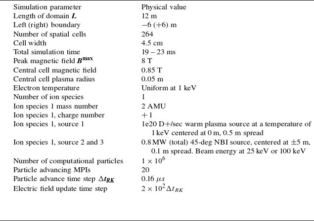
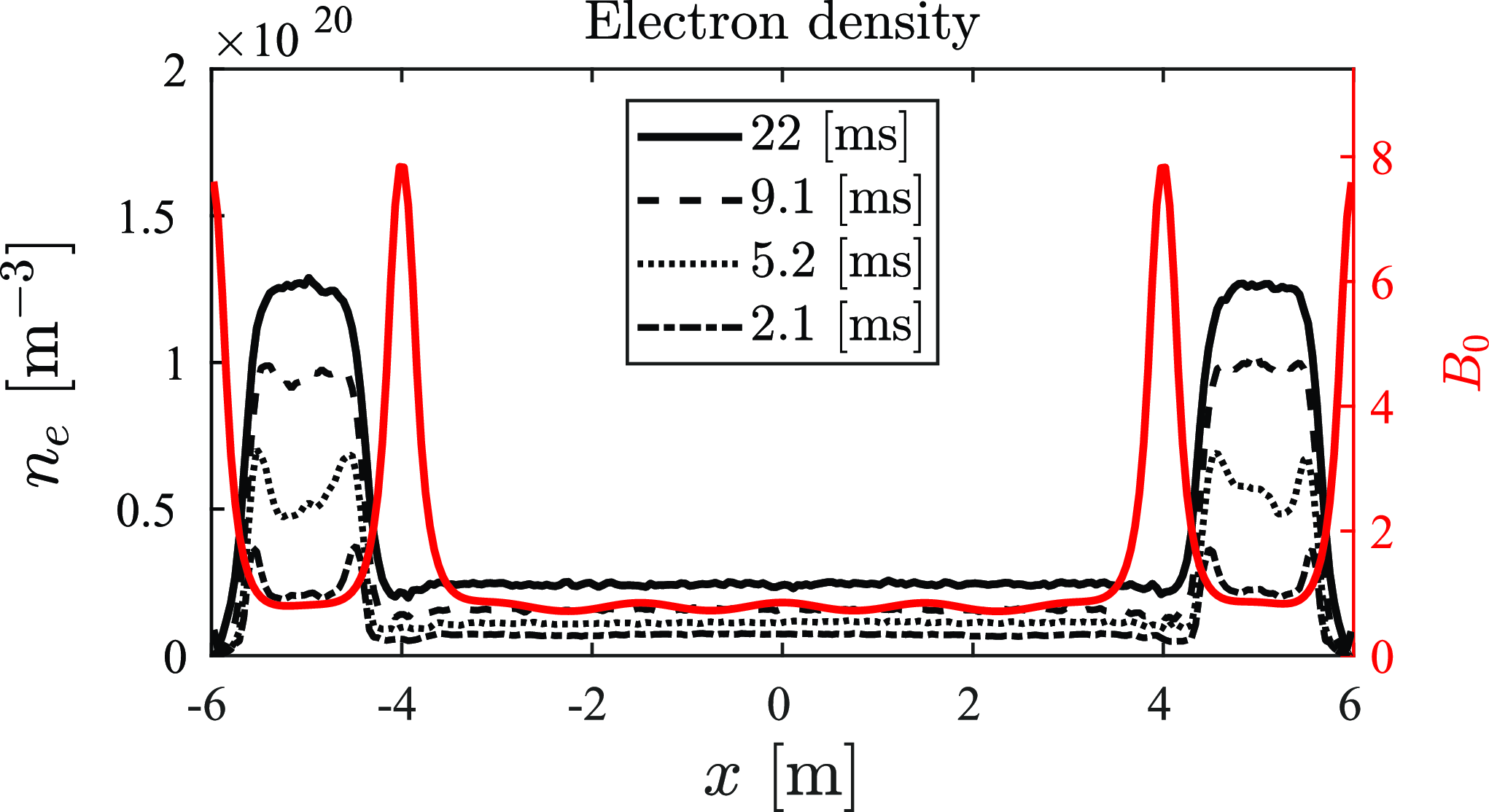
Figure 1. Electron density (black) along the length of the device for various simulation times (see legend). The magnetic field strength along the length of the computational domain is represented by the red trace. The NBI energy in each end-plug is 25 keV at 0.4 MW.
3.2. 25 keV beam case
The simulation is started with a uniform electron density of $5\times 10^{18}\rm m^{-3}$
. Neutral beams are injected into the end-plugs at 45 degrees relative to the magnetic field at energy 25 keV from the start of the simulation. This case is evolved up to 22 ms. The electron density profile at various time steps is presented in figure 1. Temporal evolution of the electron density in the end-plugs (x = 5 m) and the central cell is presented in figure 2 showing beam thermalization, whereas the central cell density (x = 0 m) is still evolving.
$5\times 10^{18}\rm m^{-3}$
. Neutral beams are injected into the end-plugs at 45 degrees relative to the magnetic field at energy 25 keV from the start of the simulation. This case is evolved up to 22 ms. The electron density profile at various time steps is presented in figure 1. Temporal evolution of the electron density in the end-plugs (x = 5 m) and the central cell is presented in figure 2 showing beam thermalization, whereas the central cell density (x = 0 m) is still evolving.
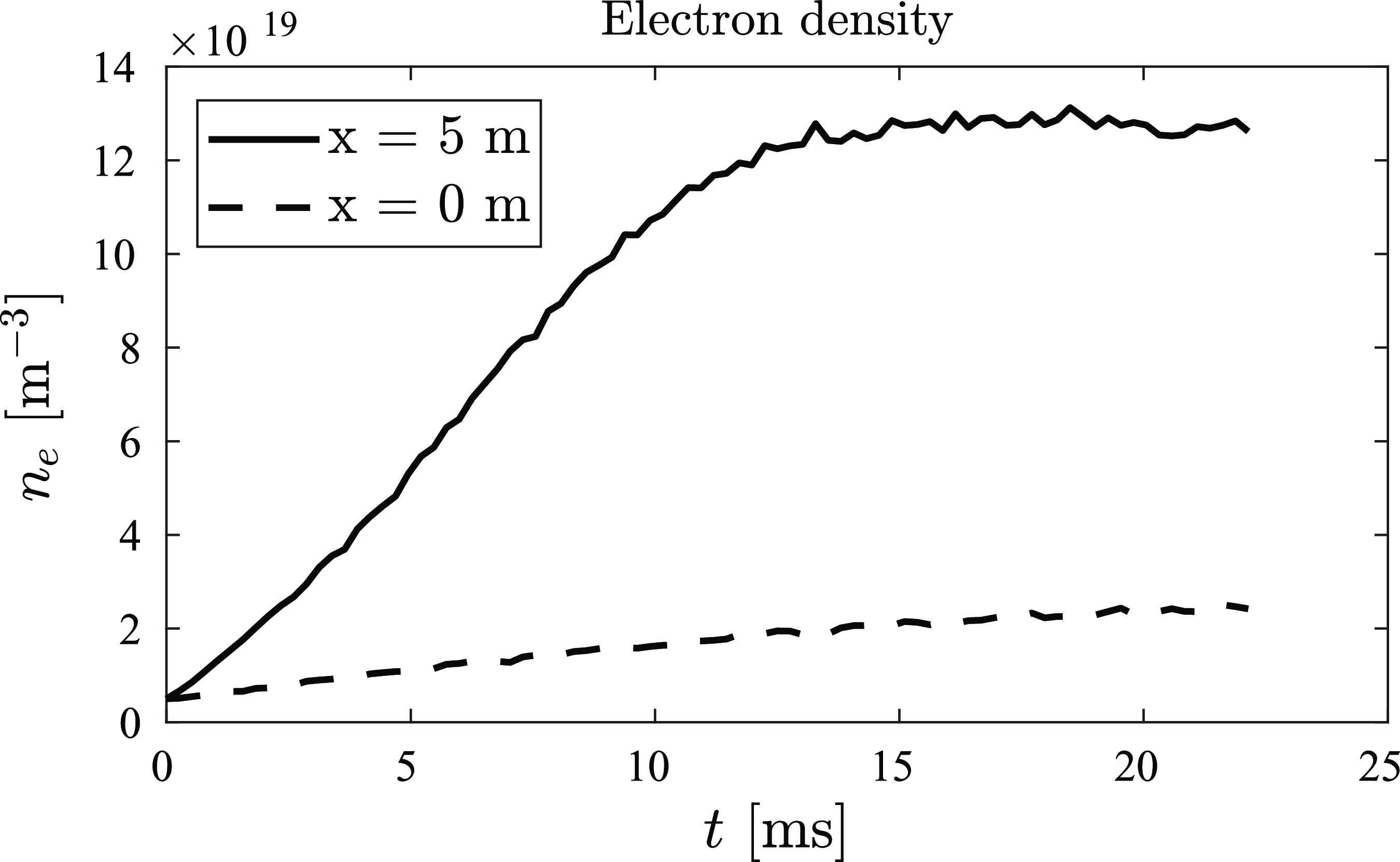
Figure 2. Electron density temporal evolution in the central cell (dashed) and end-plug (solid) region. The NBI energy in each end-plug is 25 keV at 0.4 MW.
The increase in density in the end-plugs is caused by accumulation of a sloshing ion population driven by the 45-degree neutral beams. At early times (5 ms), the formation of sloshing ion density peaks at the turning points can be clearly observed in figure 1. As density and time increases, the sloshing ion population accumulates pitch angle scattering, begins to thermalize, and eventually form a single density peak in the end-plug regions, saturating at a value of $1.2\times 10^{20}\rm m^{-3}$
in about 15 ms. Beyond that time, the source of fast ions equals the scattering of fast ions out of the end-plugs.
$1.2\times 10^{20}\rm m^{-3}$
in about 15 ms. Beyond that time, the source of fast ions equals the scattering of fast ions out of the end-plugs.
The time-dependent ion temperatures (parallel and perpendicular) in the end-plugs are presented in figure 3. Perpendicular temperature is taken at the sloshing ion turning point while the parallel temperature is taken at the center of the end-plug where the parallel energy of the sloshing ions is maximum. At the very early stages of the simulation when the density is low, both the parallel and perpendicular temperature quickly increase to values close to the injection energy of the beams. As time progresses, density accumulation increases the collisionality of the beams and eventually thermalization at a lower temperature is reached at around 15 ms.
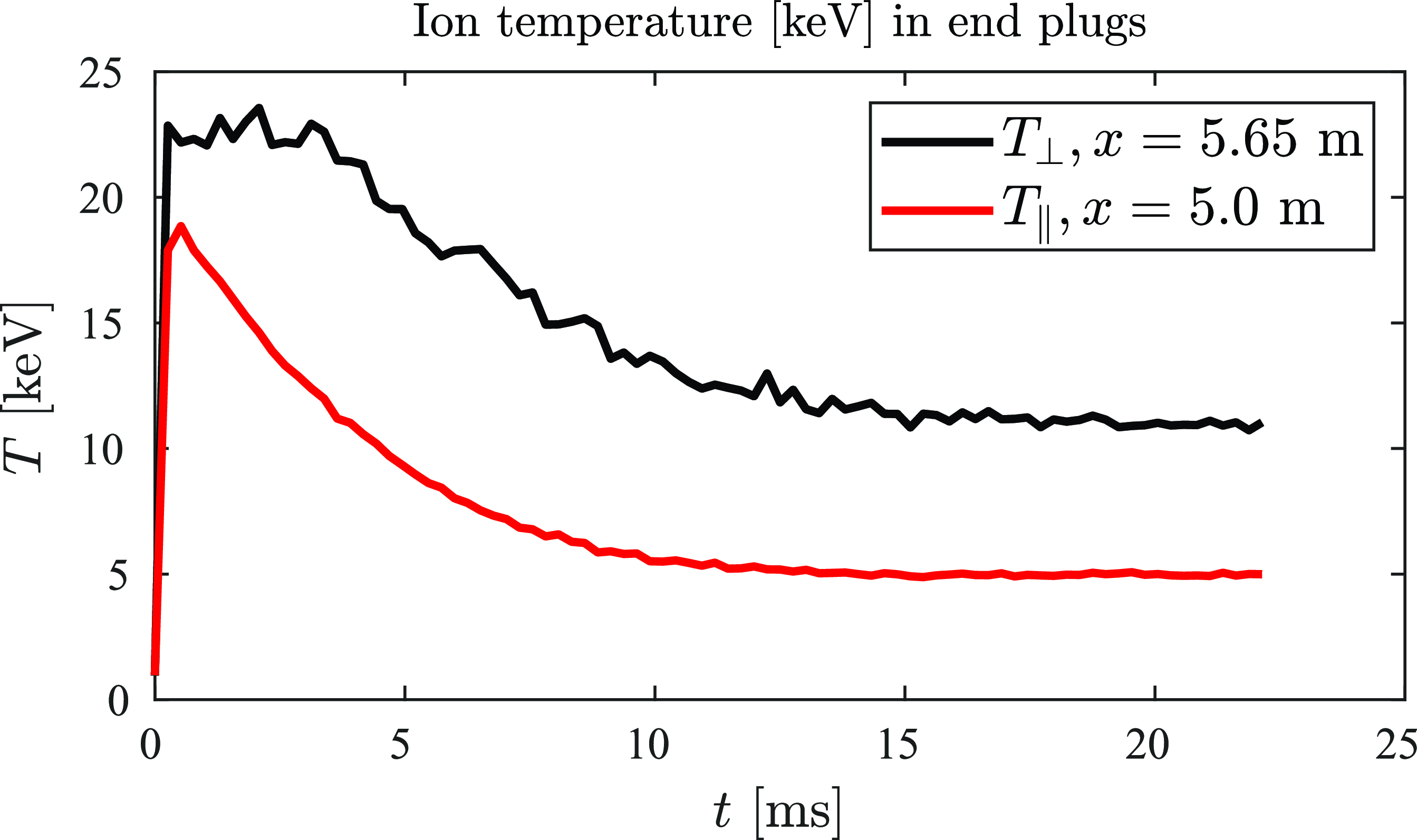
Figure 3. Parallel (red) and perpendicular (black) ion temperatures in the end-plugs. The perpendicular and parallel temperature is taken at the turning point of the sloshing ions density and mid plane of end-plugs respectively. The NBI energy in each end-plug is 25 keV at 0.4 MW.
It is worth noting from figure 2 that the density in the central cell increases linearly throughout the entire simulation. As the density in the end-plugs increase, the confinement of the central cell plasma improves due to the formation of the electrostatic confinement potential ${\unicode[Arial]{x0394}} V=V_{ep}-V_{cc}$
where the subscripts ‘ep’ and ‘cc’ refer to end-plugs and central cell respectively. The electric potential associated with the plasma density profile at 22 ms is presented in figure 4 below. The potential difference between the central cell and the end-plugs
${\unicode[Arial]{x0394}} V=V_{ep}-V_{cc}$
where the subscripts ‘ep’ and ‘cc’ refer to end-plugs and central cell respectively. The electric potential associated with the plasma density profile at 22 ms is presented in figure 4 below. The potential difference between the central cell and the end-plugs ${\unicode[Arial]{x0394}} V$
is approximately 1.7
${\unicode[Arial]{x0394}} V$
is approximately 1.7 $T_{e}$
or 1.7 kV. For a central cell ion temperature of about 1 keV, this electrostatic potential can confine a large fraction of the warm plasma in the central cell. This will be shown more clearly with the presentation of the ion distribution function later in the paper.
$T_{e}$
or 1.7 kV. For a central cell ion temperature of about 1 keV, this electrostatic potential can confine a large fraction of the warm plasma in the central cell. This will be shown more clearly with the presentation of the ion distribution function later in the paper.
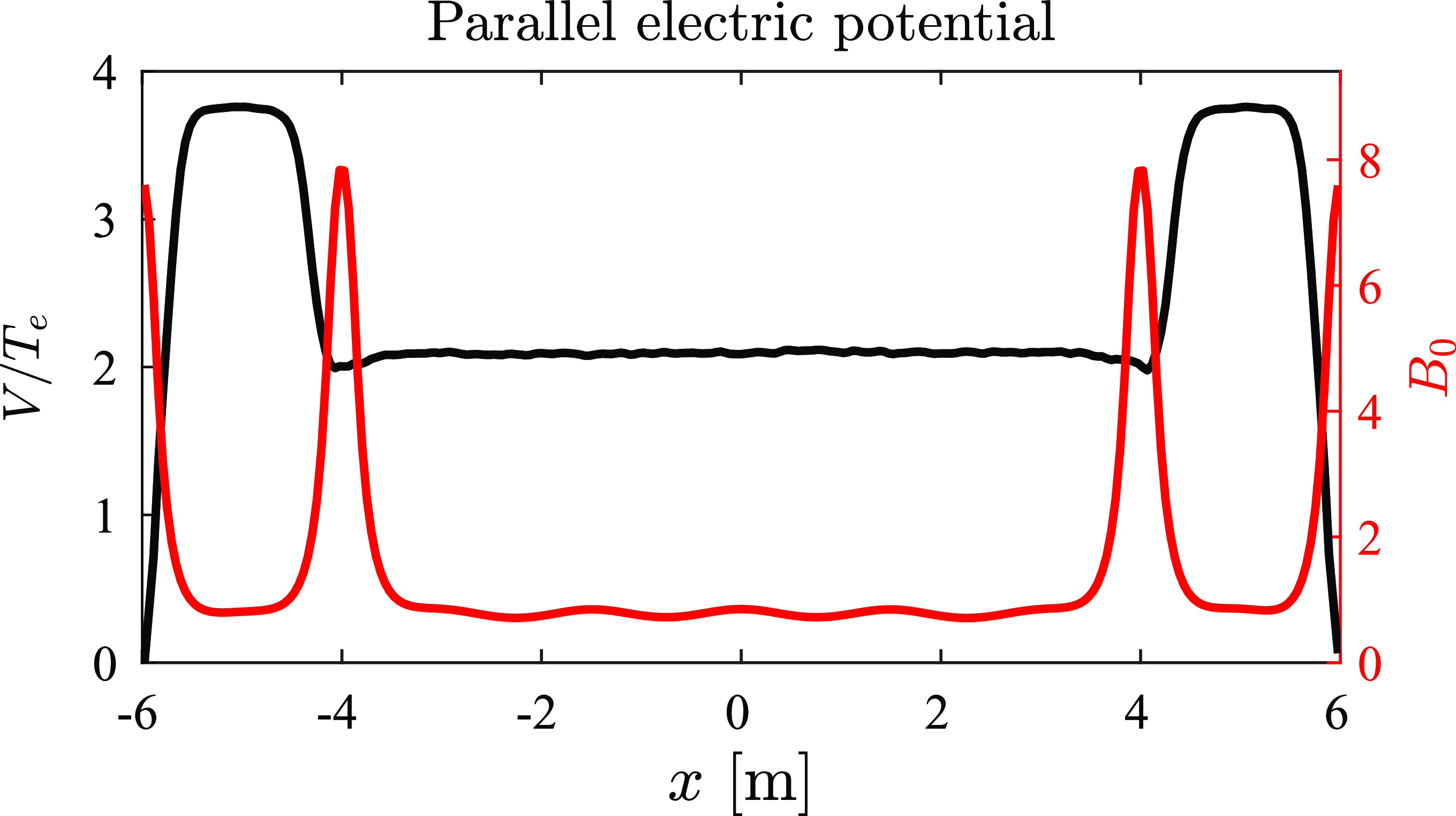
Figure 4. Parallel electric potential (black) and magnetic field strength (red) along the length of the device. The electron temperature is taken to be uniform at a value of 1 keV. The NBI energy in each end-plug is 25 keV at 0.4 MW.
Let us now consider the ion confinement time in the central cell given the conditions observed in the simulation (potential difference, plasma density, ion temperature). To carry this out, we use equations (2.2) and (2.3) from reference (Rognlien and Cutler Reference Rognlien and Cutler1980) for the confinement time $\tau _{i}$
for a singly-charged ion in a square electrostatic well. These equations are presented in (3.1) and (3.2), where
$\tau _{i}$
for a singly-charged ion in a square electrostatic well. These equations are presented in (3.1) and (3.2), where $\tau _{ii}$
is the ion-ion scattering time,
$\tau _{ii}$
is the ion-ion scattering time, $R$
the mirror ratio and
$R$
the mirror ratio and $T_{ic}$
the ion temperature in the central cell. Letting
$T_{ic}$
the ion temperature in the central cell. Letting $T_{ic}=$
1 keV,
$T_{ic}=$
1 keV, $n=3-4\times 10^{19}\,\mathrm{m}^{-3}$
and
$n=3-4\times 10^{19}\,\mathrm{m}^{-3}$
and $m_{i}=2m_{p}$
, we get an ion-ion scattering time
$m_{i}=2m_{p}$
, we get an ion-ion scattering time $\tau _{ii}$
of about 1–1.4 ms. Given the mirror ratio (R = 9) and the potential difference (
$\tau _{ii}$
of about 1–1.4 ms. Given the mirror ratio (R = 9) and the potential difference ( ${\unicode[Arial]{x0394}} V=1.7$
keV), the Pastukhov confinement time
${\unicode[Arial]{x0394}} V=1.7$
keV), the Pastukhov confinement time $\tau _{i}$
falls between 21 and 29 ms.
$\tau _{i}$
falls between 21 and 29 ms.
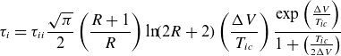 \begin{equation}\tau _{i}=\tau _{ii}\frac{\sqrt{\pi }}{2}\left(\frac{R+1}{R}\right)\ln\! (2R+2)\left(\frac{{\unicode[Arial]{x0394}} V}{T_{ic}}\right)\frac{\exp \left(\frac{{\unicode[Arial]{x0394}} V}{T_{ic}}\right)}{1+\left(\frac{T_{ic}}{2{\unicode[Arial]{x0394}} V}\right)}\end{equation}
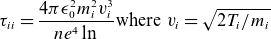 \begin{align}\tau _{ii}=\frac{4\pi \epsilon _{0}^{2}m_{i}^{2}v_{i}^{3}}{ne^{4}\ln {\unicode[Arial]{x039B}} }\text{where }v_{i}=\sqrt{2T_{i}/m_{i}}\\[-3pt]\nonumber\end{align}
We now compare the above Pastukhov confinement time estimates (21 and 29 ms) with the results from the simulation. To do this, we calculate the temporal evolution of the plasma density in the central cell and select the confinement time that best fits the results from PICOS++. The expression that describes this process is given in (3.3) (Kumar et al. Reference Kumar, Caneses-Marin, Lau and Goulding2023), where the mean plasma density in the central cell is represented by $n$
, the particle generation rate by
$n$
, the particle generation rate by $G$
, the central cell length by
$G$
, the central cell length by $L$
, the mean cross sectional area of the central cell
$L$
, the mean cross sectional area of the central cell $A$
and the confinement time by
$A$
and the confinement time by $\tau _{i}$
. In this formulation we have used the approximation that the plasma density is practically uniform in the central cell as shown in figure 1. For a constant particle generation rate
$\tau _{i}$
. In this formulation we have used the approximation that the plasma density is practically uniform in the central cell as shown in figure 1. For a constant particle generation rate $G$
, the solution to (3.3) is given in (3.4). The steady state solution (
$G$
, the solution to (3.3) is given in (3.4). The steady state solution ( $t\rightarrow \infty$
) is given in (3.5).
$t\rightarrow \infty$
) is given in (3.5).
Using a constant particle generation rate of $1\times 10^{20}$
particles per second (table 1), the temporal evolution of the plasma density in the central cell is compared with the results from PICOS++ in figure 5. The black trace represents the numerical data produced with PICOS++. The red trace is calculated using (3.3) with a confinement time of 24 ms which leads to the best fit to the numerical results. The horizontal red broken trace represents the steady state plasma density using (3.5). This comparison shows that the confinement time required to fit (3.3) to the numerical result (
$1\times 10^{20}$
particles per second (table 1), the temporal evolution of the plasma density in the central cell is compared with the results from PICOS++ in figure 5. The black trace represents the numerical data produced with PICOS++. The red trace is calculated using (3.3) with a confinement time of 24 ms which leads to the best fit to the numerical results. The horizontal red broken trace represents the steady state plasma density using (3.5). This comparison shows that the confinement time required to fit (3.3) to the numerical result ( $\tau _{i}=24\,\mathrm{ms}$
) is consistent to the confinement time calculated using the Pastukhov expression (
$\tau _{i}=24\,\mathrm{ms}$
) is consistent to the confinement time calculated using the Pastukhov expression ( $\tau _{i}=21\text{to }29\text{ ms}$
) (3.1).
$\tau _{i}=21\text{to }29\text{ ms}$
) (3.1).
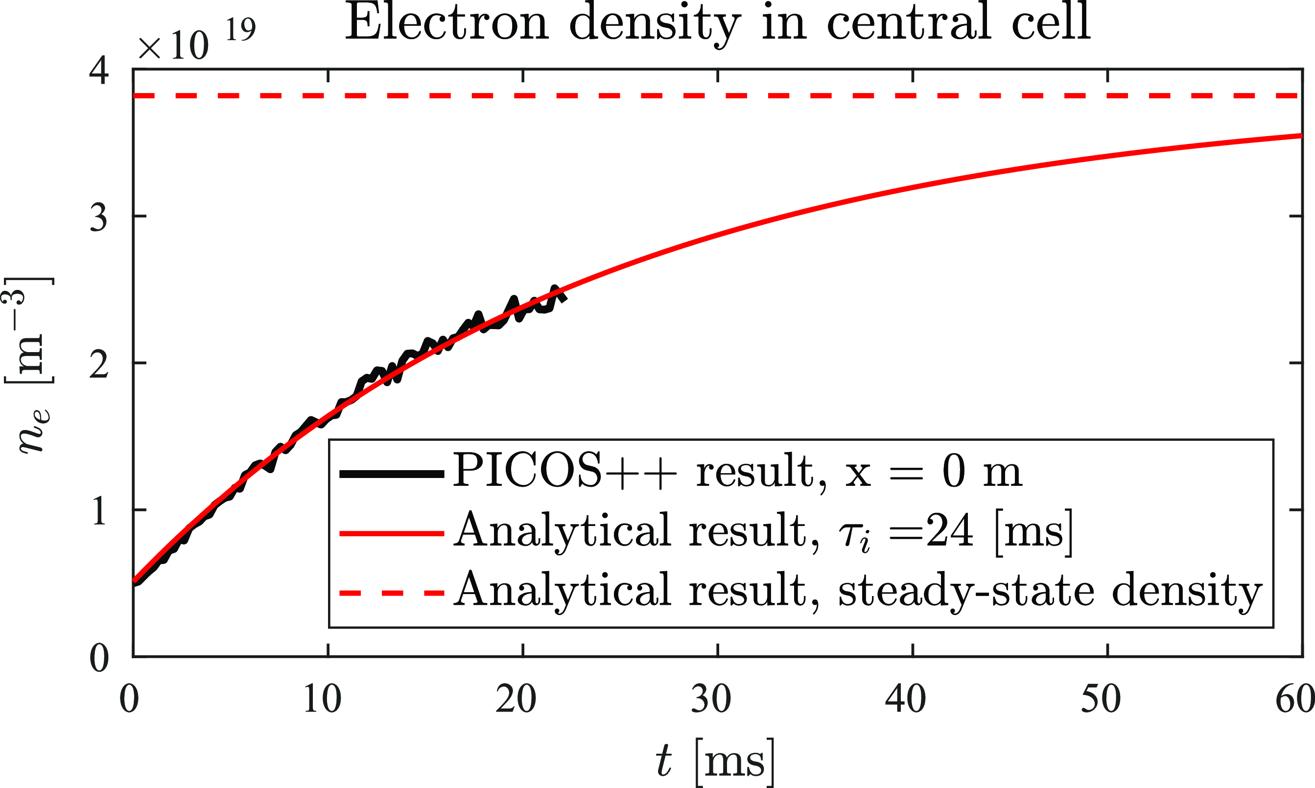
Figure 5. Temporal evolution of the central cell density calculated by PICOS++ (black) and analytical solution (red) using a confinement time of 24 ms. The red-dotted line represents the steady state value that is expected given the confinement time and particle generation rate.
 \begin{equation}\dot{n}+\frac{n}{\tau _{i}}=\frac{G}{LA}\end{equation}
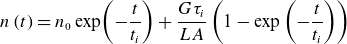 \begin{equation}n\left(t\right)=n_{0}\exp \!\left(-\frac{t}{t_{i}}\right)+\frac{G\tau _{i}}{LA}\left(1-\exp \left(-\frac{t}{t_{i}}\right)\right)\end{equation}
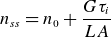 \begin{equation}n_{ss}=n_{0}+\frac{G\tau _{i}}{LA}\end{equation}
At the edges of the computational domain, the potential drop between the center of the end-plug and the throat at the edge of the domain is close to 3.8 $T_{e}$
. This potential drop accelerates ions towards the edge of the domain as shown in figure 6 to speeds approaching the ion sound speed given by
$T_{e}$
. This potential drop accelerates ions towards the edge of the domain as shown in figure 6 to speeds approaching the ion sound speed given by $c_{S}=\sqrt{e(T_{e}+T_{i})/m_{i}}$
. To model the complete effect of the sheath, the potential drop at the wall needs to be set to make the ion flux equal to the electron flux retarded by the potential drop in the bulk plasma and sheath region. At present this sheath potential drop is not modeled; however, it is important to note that a large potential drop is produced at the edge of the domain in the quasi-neutral region between the center of the end-plug and the magnetic throat at the edge of the domain. This potential drop accelerates ions in the quasi-neutral region up to speeds approaching the ion sound speed. This reduces the potential drop required at the sheath region to achieve ambipolarity.
$c_{S}=\sqrt{e(T_{e}+T_{i})/m_{i}}$
. To model the complete effect of the sheath, the potential drop at the wall needs to be set to make the ion flux equal to the electron flux retarded by the potential drop in the bulk plasma and sheath region. At present this sheath potential drop is not modeled; however, it is important to note that a large potential drop is produced at the edge of the domain in the quasi-neutral region between the center of the end-plug and the magnetic throat at the edge of the domain. This potential drop accelerates ions in the quasi-neutral region up to speeds approaching the ion sound speed. This reduces the potential drop required at the sheath region to achieve ambipolarity.
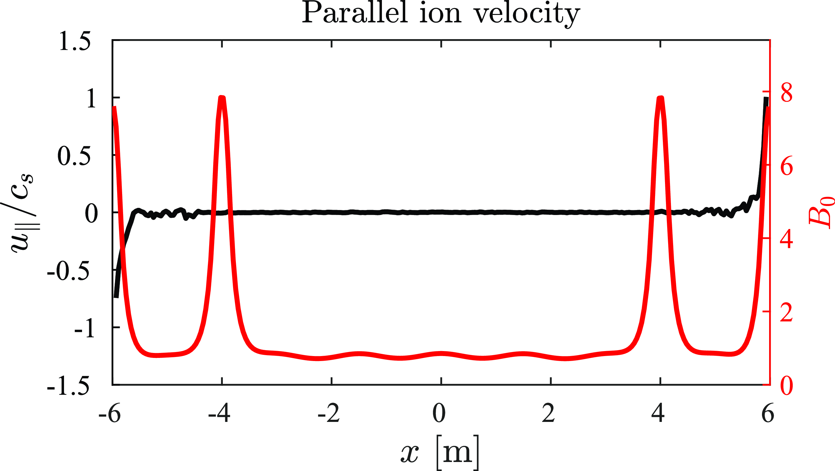
Figure 6. Parallel ion velocity (black) and magnetic field strength (red) along the length of the device. The electron temperature is taken to be uniform at a value of 1 keV.
The ion distribution function in the central cell in figure 7 is assembled by integrating the region $x_{m}=$
−4 to + 4 m. The black solid line represents the trapped-passing boundary with the effect of the electric potential given by (3.6), where
$x_{m}=$
−4 to + 4 m. The black solid line represents the trapped-passing boundary with the effect of the electric potential given by (3.6), where ${\unicode[Arial]{x0394}} V$
is the potential difference between the central cell and the maximum potential in the end-plug at x = 5 m. Due to the sign of the potential (positive), the trapped-passing boundary crosses the horizontal axis at values of
${\unicode[Arial]{x0394}} V$
is the potential difference between the central cell and the maximum potential in the end-plug at x = 5 m. Due to the sign of the potential (positive), the trapped-passing boundary crosses the horizontal axis at values of $v_{\parallel }=\pm \sqrt{2e{\unicode[Arial]{x0394}} V/M}$
. If we normalize this quantity by a characteristic ion thermal velocity
$v_{\parallel }=\pm \sqrt{2e{\unicode[Arial]{x0394}} V/M}$
. If we normalize this quantity by a characteristic ion thermal velocity $v_{T}=\sqrt{2eT/M}$
we get
$v_{T}=\sqrt{2eT/M}$
we get $v_{\parallel }/v_{T}=\pm \sqrt{{\unicode[Arial]{x0394}} V/T}$
which defines the region in velocity space confined by the electrostatic potential. Given the potential difference
$v_{\parallel }/v_{T}=\pm \sqrt{{\unicode[Arial]{x0394}} V/T}$
which defines the region in velocity space confined by the electrostatic potential. Given the potential difference ${\unicode[Arial]{x0394}} V\approx$
1.7 keV between the central cell and end-plug and an ion temperature in that region of about 1 keV, we get
${\unicode[Arial]{x0394}} V\approx$
1.7 keV between the central cell and end-plug and an ion temperature in that region of about 1 keV, we get $v_{\parallel }/v_{T}=1.28$
.
$v_{\parallel }/v_{T}=1.28$
.
 \begin{equation}v_{\parallel }^{2}=v_{\bot }^{2}\left(R-1\right)+\frac{2e{\unicode[Arial]{x0394}} V}{M}\end{equation}
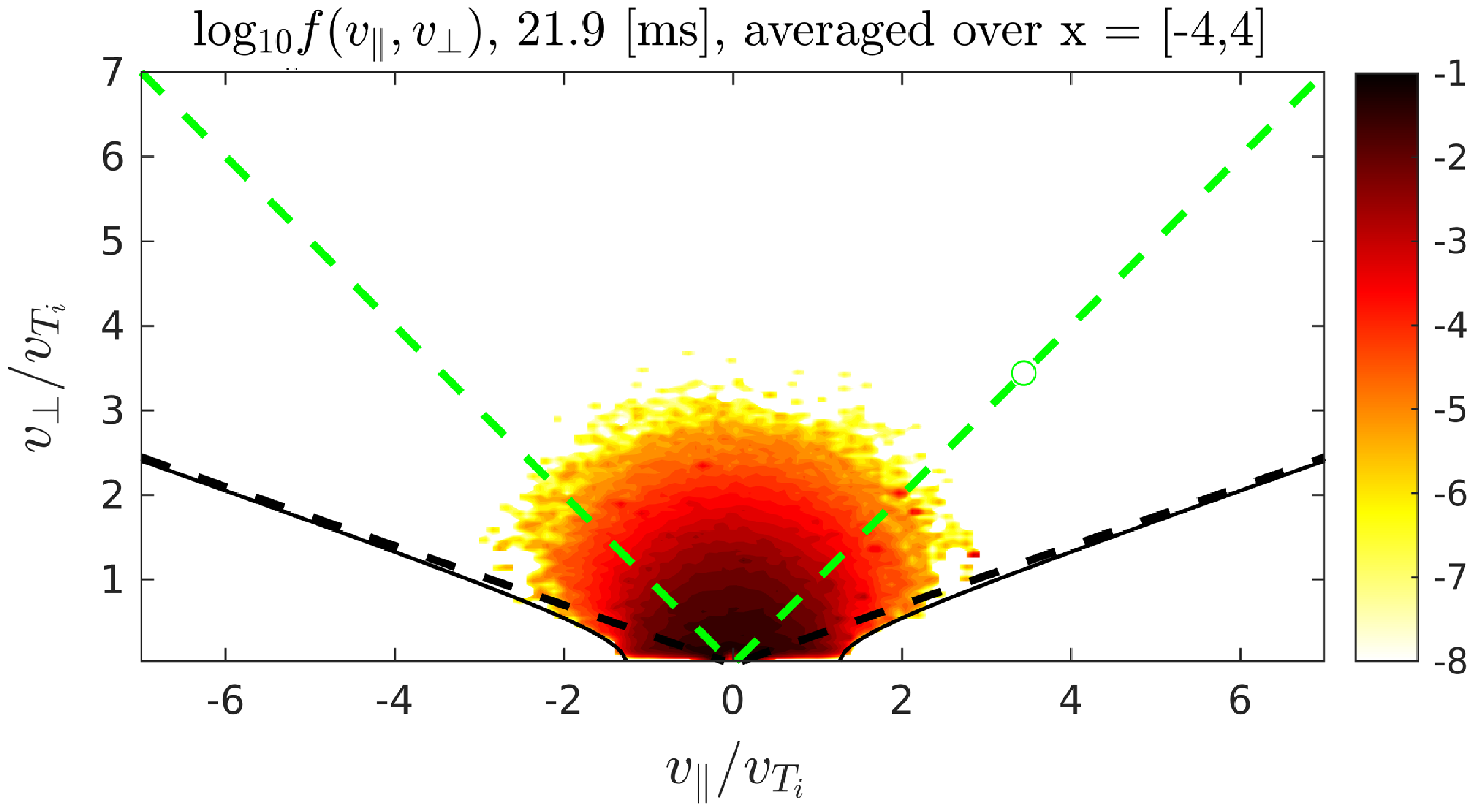
Figure 7. Ion distribution function in the central cell averaged over region −4 to + 4 m at 21.9 ms. The black dotted and solid lines represent the trapped-passing boundary without and with the effect of the electrostatic potential respectively. The solid line indicates that a fraction of the low energy thermal ions is effectively confined by the electrostatic potential between the central cell and the end-plug as shown in figure 4. The NBI energy in each end-plug is 25 keV at 0.4 MW.
The distribution function in the end-plugs is shown in figure 8. The top shows the sloshing ions at early times. The black solid line represents the trapped-passing boundary with the effect of the electrostatic potential given by (3.6). In this case, the potential difference is between the end-plug maximum and the throat at the edge of the domain. It is negative and accelerates low energy ions out of the end-plug. This empties the low energy portion of the distribution function which is re-populated via collisional diffusion from the confined region. Everything above the hyperbolic trapped-passing boundary is confined (electrostatic and magnetic) in the end-plugs.
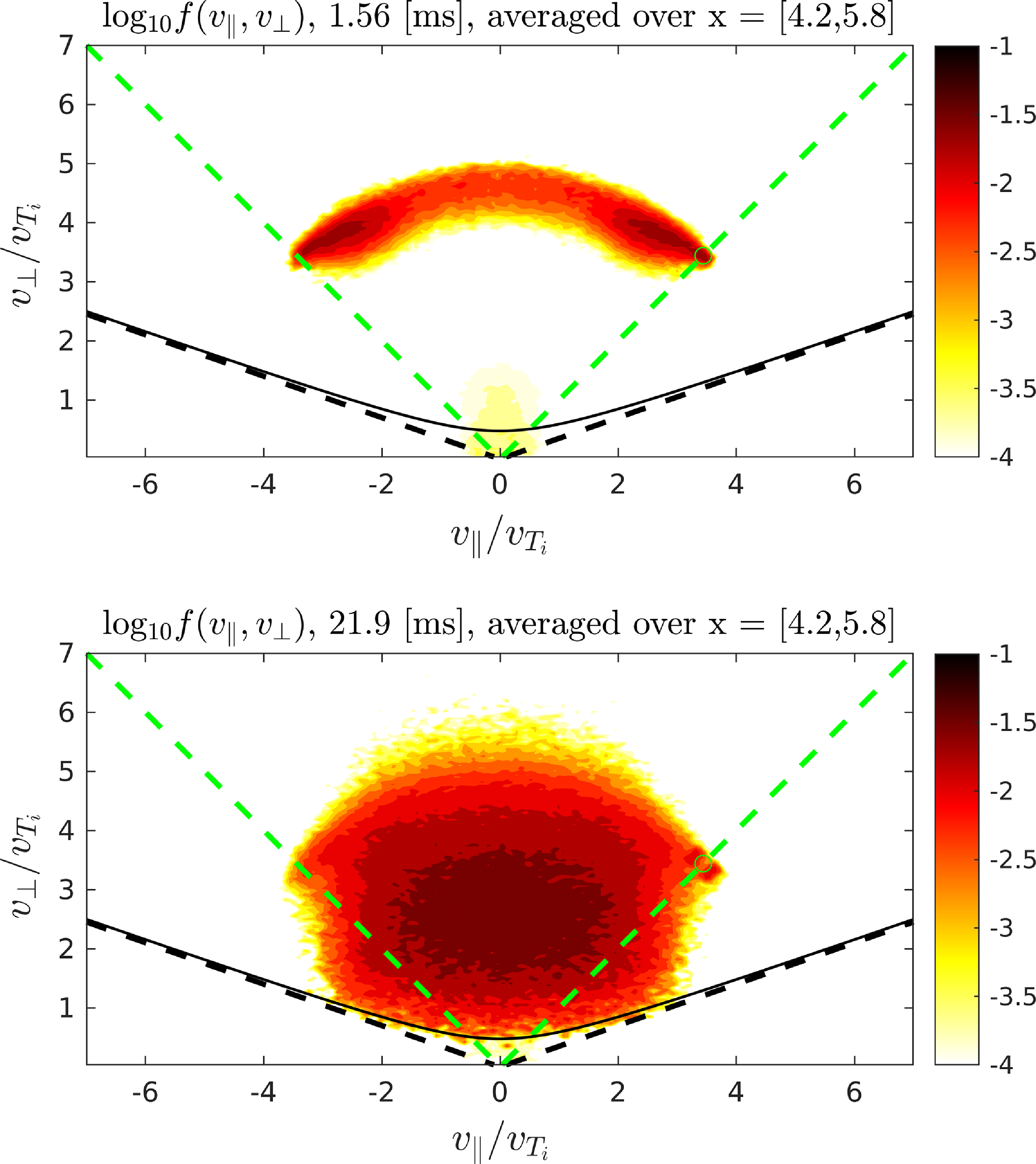
Figure 8. Ion distribution function in the end-plugs at 1.56 ms (top) and 21.9 ms (bottom) averaged over region $x_{m}=5m\pm 0.8m$
. The black solid and dotted lines represent the trapped-passing boundary with and without the effect of the electrostatic potential, respectively. The green dotted lines represent the NBI injection angle (45 degrees). The NBI energy in each end-plug is 25 keV and power is 0.4 MW.
$x_{m}=5m\pm 0.8m$
. The black solid and dotted lines represent the trapped-passing boundary with and without the effect of the electrostatic potential, respectively. The green dotted lines represent the NBI injection angle (45 degrees). The NBI energy in each end-plug is 25 keV and power is 0.4 MW.
3.3. 100 keV beam case
This case is identical to the previous case except 100 keV beams are used. Neutral beams are injected into the end-plugs at 45 degrees relative to the magnetic field as per table 1 from the start of the simulation. This case is evolved up to 23 ms, less than the thermalization time. The electron density profile at various time steps is presented in figure 9. Temporal evolution in the end-plugs (x = 5 m) and in the central cell (x = 0 m) is shown in figure 10.
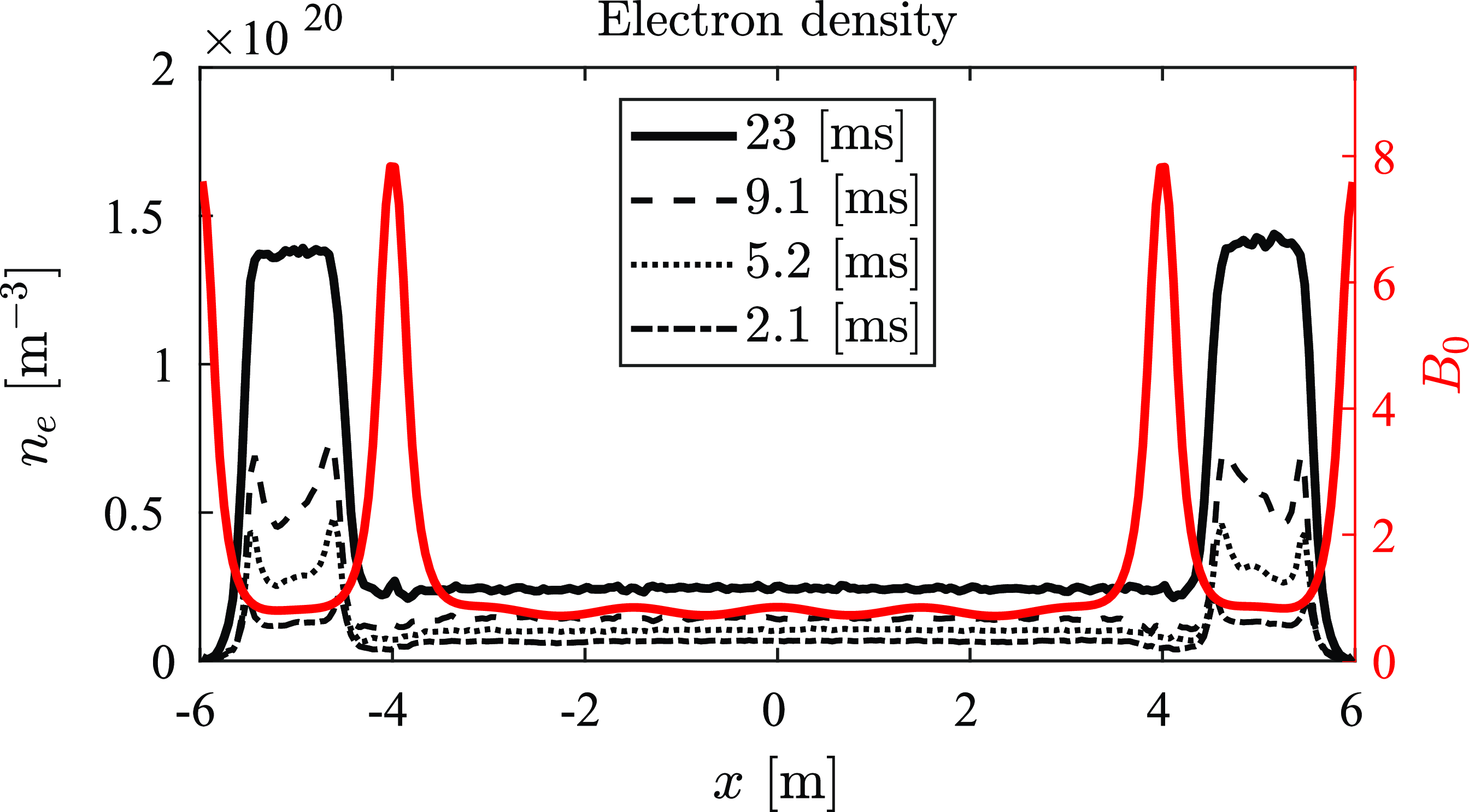
Figure 9. Electron density (black) along the length of the device for various simulation times (see legend). The magnetic field strength along the length of the computational domain is represented by the red trace. The NBI energy in each end-plug is 100 keV at 0.4 MW.
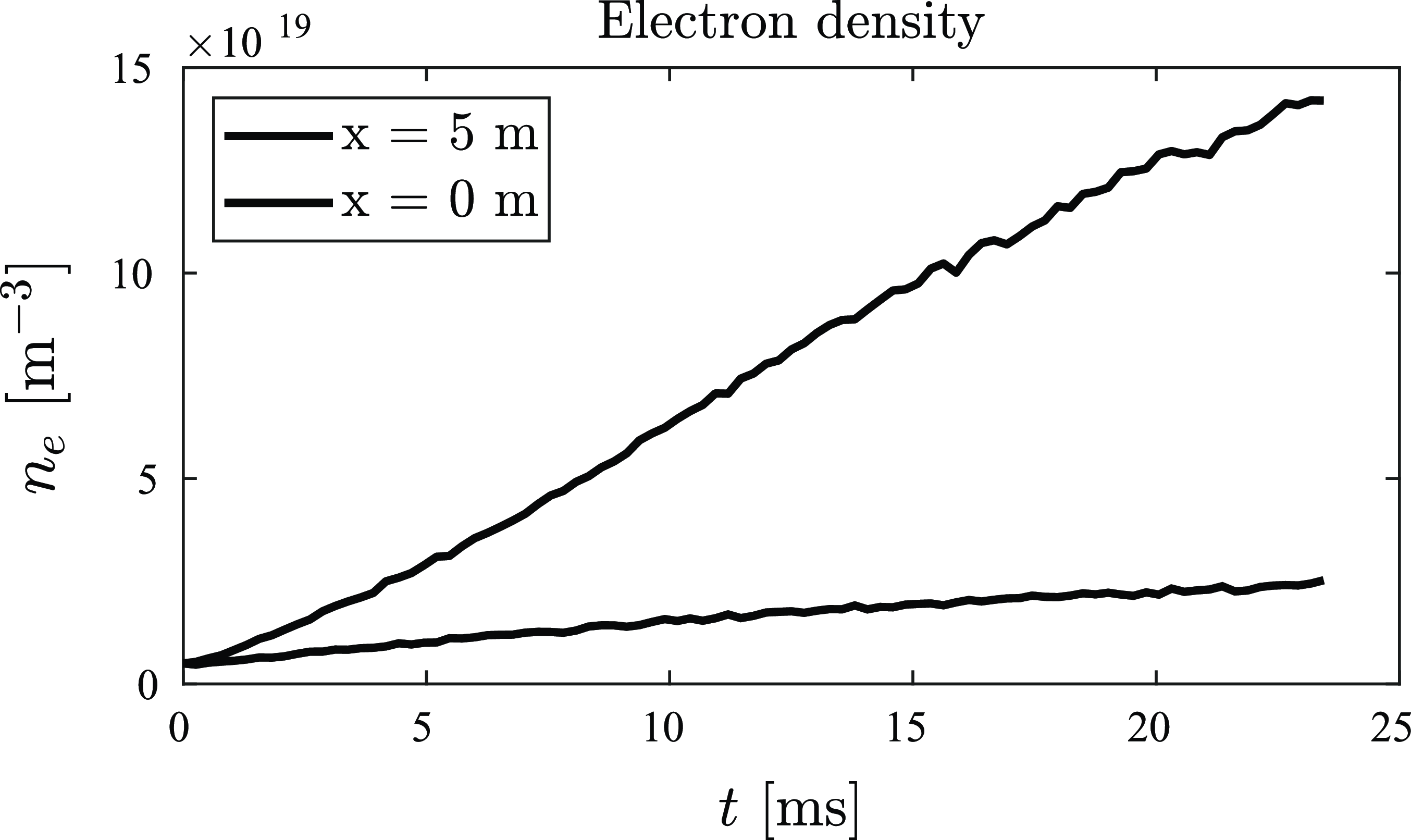
Figure 10. Electron density temporal evolution in the central cell (dashed) and end-plug (solid) region. The NBI energy in each end-plug is 100 keV at 0.4 MW.
Temporal evolution of the ion temperature in the end-plugs is shown in figure 11. Perpendicular temperature is close to the injection energy of 100 keV and remains steady up to about 15 ms and then starts to drop indicating the beginning of the thermalization process.
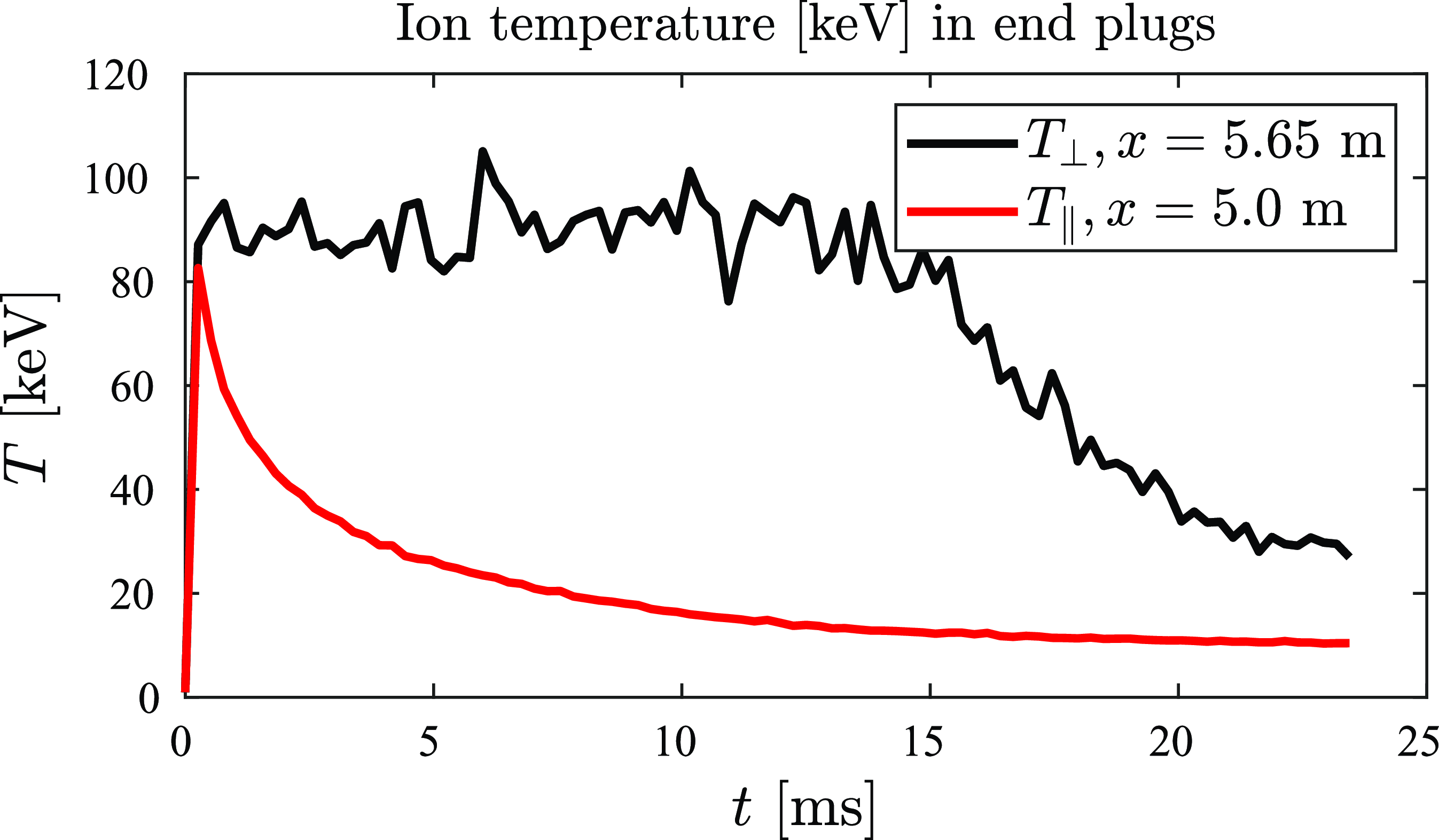
Figure 11. Parallel (red) and perpendicular (black) ion temperatures in the end-plugs. The perpendicular and parallel temperature is taken at the turning point of the sloshing ions density and mid plane of end-plugs respectively. The NBI energy in each end-plug is 100 keV at 0.4 MW.
The electric potential associated with the plasma density profile in figure 9 at 23 ms is presented in figure 12 below. Despite the higher NBI energy (100 keV), the potential difference between the central cell and the end-plugs is approximately 1.8 $T_{e}$
or 1.8 keV which is only slightly higher than in the 25 keV case. How this happens remains unclear. We speculate that the use of a fully non-linear Fokker-Planck collision operator including the electrons will modify this result. As the beam slows down, it heats the electrons and this in turn reduces the drag on the fast ions on electrons thus increasing the confinement of the beam and the sloshing ion density. The increased end-plug density would increase the potential difference. The ion distribution function in the central cell for this 100 keV case looks very similar to that presented in figure 8 except for the small change in the trapped-passing boundary intercept where
$T_{e}$
or 1.8 keV which is only slightly higher than in the 25 keV case. How this happens remains unclear. We speculate that the use of a fully non-linear Fokker-Planck collision operator including the electrons will modify this result. As the beam slows down, it heats the electrons and this in turn reduces the drag on the fast ions on electrons thus increasing the confinement of the beam and the sloshing ion density. The increased end-plug density would increase the potential difference. The ion distribution function in the central cell for this 100 keV case looks very similar to that presented in figure 8 except for the small change in the trapped-passing boundary intercept where $v_{\parallel }/v_{T}=1.33$
.
$v_{\parallel }/v_{T}=1.33$
.

Figure 12. Parallel electric potential (black) and magnetic field strength (red) along the length of the device. The electron temperature is taken to be uniform at a value of 1 keV. The NBI energy in each end-plug is 100 keV at 0.4 MW.
3.4. Effect of the end-plug electron temperature
In this section, we investigate the effect of increasing the end-plug electron temperature ( $T_{ep}$
) relative to that in the central cell (
$T_{ep}$
) relative to that in the central cell ( $T_{ec}$
) on the electric potential and the central cell confinement.
$T_{ec}$
) on the electric potential and the central cell confinement.
3.4.1. Numerical results
PICOS++ simulations were performed with 25 keV NBI as per the conditions in table 1; however, a new feature was introduced: the electron temperature in the end-plugs was systematically increased while keeping the central cell electron temperature the same at 1 keV as illustrated in figure 13. The electron density profiles along the length of the computational domain at the end of the simulations (22 ms) for the different electron temperature scenarios are presented in figure 14. The associated electric potential profiles are presented in figure 15. The results show an increase in density in both the central cell and end-plugs. The increase in density in the end-plugs is likely caused by the reduced electron drag on the sloshing ions. The increase in density in the central cell is caused by the improved confinement time in connection with increased end-plug potentials. In § 3.4.3, the observed confinement times are compared with those predicted by the Pastukhov expression (3.1).
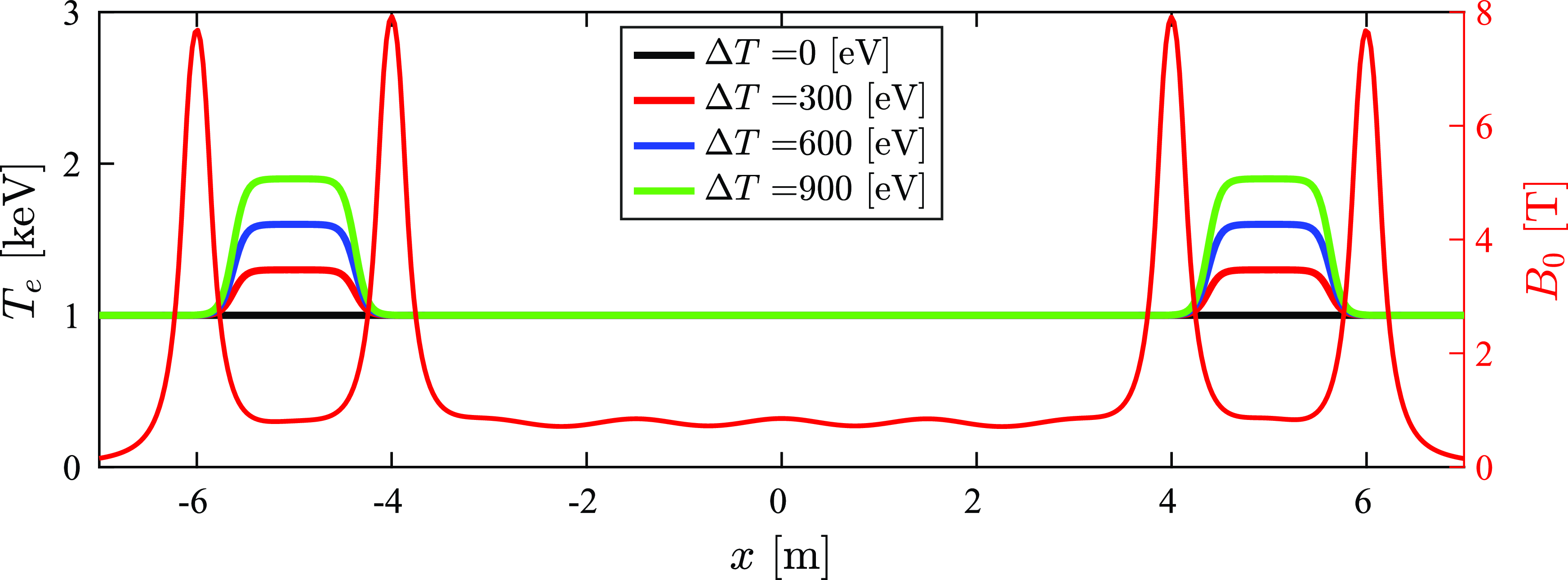
Figure 13. Electron temperature profiles where the value at the end-plugs is systematically increased to observe the effect on confinement and electrostatic potential.
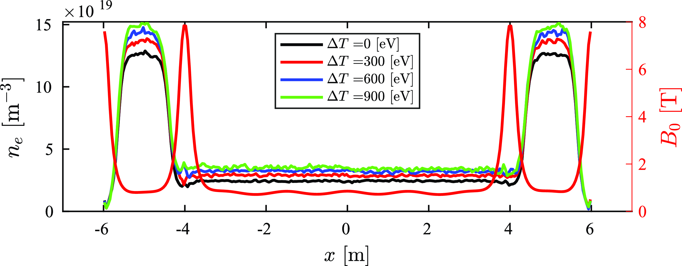
Figure 14. Electron density profiles at the end of the simulation (22 ms) for the various electron temperature profiles presented in Figure 13.
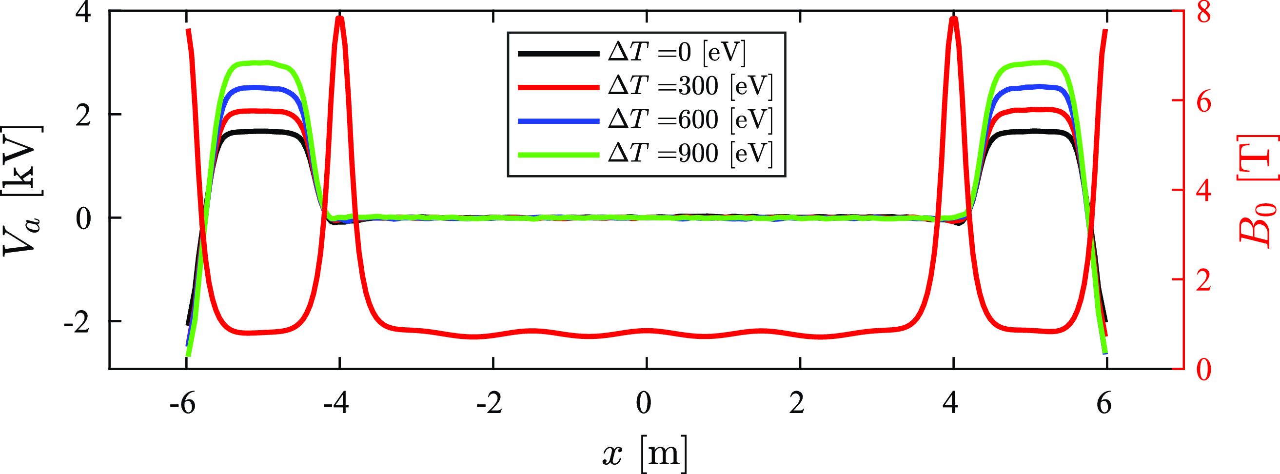
Figure 15. Parallel electric potential profiles at the end of the simulation (22 ms) for the various electron temperature profiles presented in Figure 13.
3.4.2. Electric potential scaling with temperature
To understand the effect of electron temperature differences between the central cell and the end-plugs on the formation of the electric potential, we present a simple model (B5) in Appendix B.
In this section, we compare the observed potentials with those predicted by such model. This expression (B5) is composed of two terms: (1) the first term is the standard Boltzmann response which scales with $\log (n_{ep}/n_{ec})$
, where
$\log (n_{ep}/n_{ec})$
, where $n_{ep}$
and
$n_{ep}$
and $n_{ec}$
represent the electron density in the end-plug and central cell respectively; (2) the second term describes the effect of having an electron temperature difference
$n_{ec}$
represent the electron density in the end-plug and central cell respectively; (2) the second term describes the effect of having an electron temperature difference ${\unicode[Arial]{x0394}} T_{e}$
between the central cell and end-plug and scales linearly with
${\unicode[Arial]{x0394}} T_{e}$
between the central cell and end-plug and scales linearly with ${\unicode[Arial]{x0394}} T_{e}$
. In figure 16, the observed potential differences (solid lines) are compared with those predicted by (B5) (dotted lines). Equation (B5) was evaluated by approximating the electron temperature profiles (figure 13) and electron density profiles (figure 14) with Heavyside step functions. The results show that the jump in potential between central cell and the end-plug is well described by the simple expression provided in (B5) using the Heaviside approximation; namely, the potential difference scales linearly with
${\unicode[Arial]{x0394}} T_{e}$
. In figure 16, the observed potential differences (solid lines) are compared with those predicted by (B5) (dotted lines). Equation (B5) was evaluated by approximating the electron temperature profiles (figure 13) and electron density profiles (figure 14) with Heavyside step functions. The results show that the jump in potential between central cell and the end-plug is well described by the simple expression provided in (B5) using the Heaviside approximation; namely, the potential difference scales linearly with ${\unicode[Arial]{x0394}} T_{e}$
.
${\unicode[Arial]{x0394}} T_{e}$
.

3.4.3. Confinement time
Finally, the confinement time observed numerically is compared with the confinement time predicted by the Pastukhov expression in (3.1). The results are presented in figure 17. The observed confinement time is obtained by fitting (3.4) to the time-dependent central cell density produced by PICOS++. For this comparison, we provide an upper and lower bound on the fitted confinement time. The theoretical confinement time (3.1) is evaluated and averaged during the steady-state period of the end-plug density (t > 14 ms). The comparison presented in figure 17 indicates that both the observed and theoretical confinement times are consistent and have similar scaling with respect to the normalized potential difference ${\unicode[Arial]{x0394}} V/T_{e}$
; however, at the larger potential values the numerical results appear to overestimate theoretical predictions, where the observed and predicted mean confinement times are 87 ms and 73 ms respectively. A more detailed and in-depth comparison would require running the numerical simulations to full steady-state so that the confinement time values are extracted directly from the steady-state central cell density rather than fitting the time-dependent part. This will be the subject of a future study.
${\unicode[Arial]{x0394}} V/T_{e}$
; however, at the larger potential values the numerical results appear to overestimate theoretical predictions, where the observed and predicted mean confinement times are 87 ms and 73 ms respectively. A more detailed and in-depth comparison would require running the numerical simulations to full steady-state so that the confinement time values are extracted directly from the steady-state central cell density rather than fitting the time-dependent part. This will be the subject of a future study.
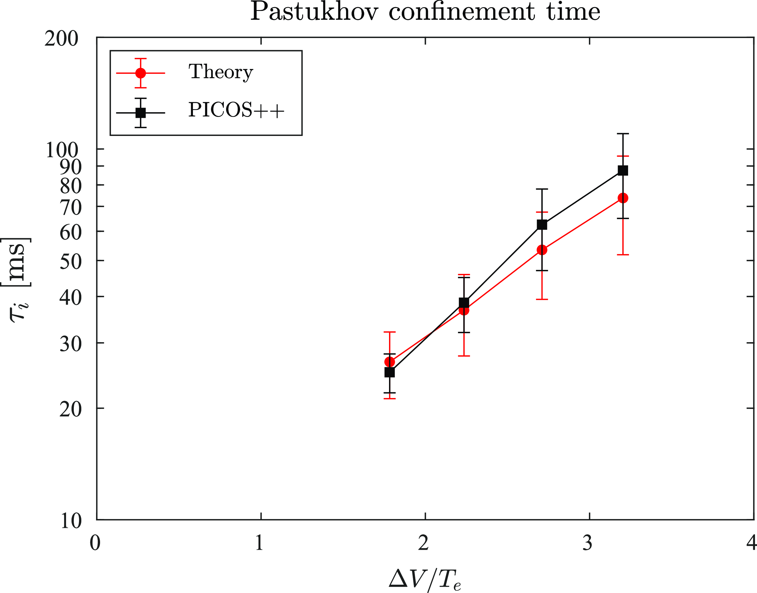
Figure 17. Comparing the numerically observed confinement times (black squares) and those predicted by (1.9) (red circles) for the various electron temperature profiles presented in figure 13.
4. Discussion
Previous work on mirror device modeling presented in reference (Endrizzi et al. Reference Endrizzi2023) makes use of the Bounce-Averaged (BA) solution of the Fokker-Planck (FP) equation using the CQL3D-m code. CQL3D-m is derived from the well-established tokamak-specific CQL3D code and adapted to mirror geometry. A key advantage of the BA formulation is that simulated times in the order of seconds are computationally readily accessible; however, in its current form, this formulation is only applicable to simple mirrors. Extensions to multiple mirror geometries such as tandem mirrors are at present being explored in CQL3D-m but not fully developed.
In this work, we demonstrate that PICOS++ can seamlessly model scenarios with multiple mirrors since the ion dynamics and associated distribution function are followed along the magnetic flux, without complications such as multiple mirror regions in CQL3D-m. In its present form, PICOS++ readily captures essential features of the tandem mirror concept; namely, electrostatic confinement of the central cell low energy ions via beam-driven, high-density, magnetically confined end-plugs. Moreover, the results from PICOS++ are consistent with the analytical expressions for the Pastukhov confinement time. However, an important limitation in the present form of PICOS++ is the lack of a fully non-linear Fokker-Planck Monte-Carlo (FPMC) collision operator. This limitation is most clearly observed when forming beam-driven sloshing ion distributions in the end-plugs. The effect of highly non-thermal distribution is not captured by the linearized Fokker-Planck operator currently in place. Incorporating a fully non-linear FP Monte-Carlo collision operation in PICOS++ is currently in progress and based on references (Wang et al. Reference Wang, Okamoto, Nakajima and Murakami1995; Takizuka and Abe Reference Takizuka and Abe1977). Once this is available, confinement/slowing down times and electric potential profile calculations can be compared with analytical expressions and results from other codes.
The next logical actions to improve the predictive capability of the code are the following: (a) enable the fully non-linear FPMC collision operator to capture beam physics more accurately, (2) develop concentrically nested flux surface solutions to capture the radial variation of the plasma and (3) develop an exhaust region solution that can be linked to the confined region solutions. The second step described above will enable us to introduce a more physics-based NBI module which makes use of radial plasma profiles and models beam capture via charge-exchange and impact ionization and shine-through. The third step is necessary to capture the electrostatic confinement of electrons which stream out of the end-plugs. In the exhaust region, ions are accelerated in the expanding magnetic field lines by the electrostatic field, whereas the electric potential reflects electrons back into the confined plasma. With sufficient field line expansion, a large fraction of electrons is reflected back into the confined region before interacting at the wall-sheath region where the presence of neutral gas can lead to electron cooling. The need here is to develop an exhaust-expander solution for both ions and electrons and connect them via boundary conditions to the solutions in the confined region produced by PICOS++, CQL3D-m or other codes.
Acknowledgements
Editor Troy Carter thanks the referees for their advice in evaluating this article.
Funding
Supported by US DOE grants US ARPA-E DE-AR0001261; DE-FG02-ER54744 and Realta Fusion.
Declaration of interests
The authors report no conflict of interest.
Appendix A.
The Monte–Carlo linearized FP collision operator used at present in PICOS++ (2.7) and (2.8) is compared with analytical expressions for the slowing down and cosine pitch angle scattering obtained from references (Hinton Reference Hinton1983; Boozer and Kuo-Petravic (Reference Boozer and Kuo-Petravic1998). The velocity of a group of particles is evolved in time using the collision operator; however, the advance particle operator is not used. The initial value problem describing the slowing down of ions in a background plasma is given by (A1), where $\nu ^{E}$
is the slowing down rate given in (92) from reference (Hinton Reference Hinton1983). Equation (A1) describes the change in kinetic energy
$\nu ^{E}$
is the slowing down rate given in (92) from reference (Hinton Reference Hinton1983). Equation (A1) describes the change in kinetic energy $E$
of an ion as it interacts with a background species with fixed conditions described in table 2. The evolution of the mean cosine pitch angle
$E$
of an ion as it interacts with a background species with fixed conditions described in table 2. The evolution of the mean cosine pitch angle $\xi =\cos (\eta )$
is described by (A2). When the mean value of the cosine pitch angle reaches zero, it indicates that the expression is dominated by the stochastic term, any memory of the starting pitch angle is lost, and any pitch angle is equally likely. The comparison between the Monte-Carlo collision operator and the analytical expressions are provided in figures 18 and 19 for the 25 keV and 100 keV case respectively.
$\xi =\cos (\eta )$
is described by (A2). When the mean value of the cosine pitch angle reaches zero, it indicates that the expression is dominated by the stochastic term, any memory of the starting pitch angle is lost, and any pitch angle is equally likely. The comparison between the Monte-Carlo collision operator and the analytical expressions are provided in figures 18 and 19 for the 25 keV and 100 keV case respectively.
 \begin{equation}\frac{{\rm d}E}{{\rm d}t}+\nu ^{E}E=0\end{equation}
 \begin{align}\frac{{\rm d}\xi }{{\rm d}t}+\nu ^{D}\xi =0\end{align}
Table 2. Simulation inputs used for the benchmarking of the collision operator with analytical expressions.
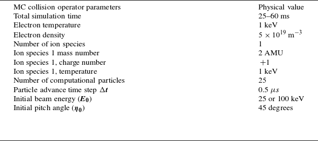
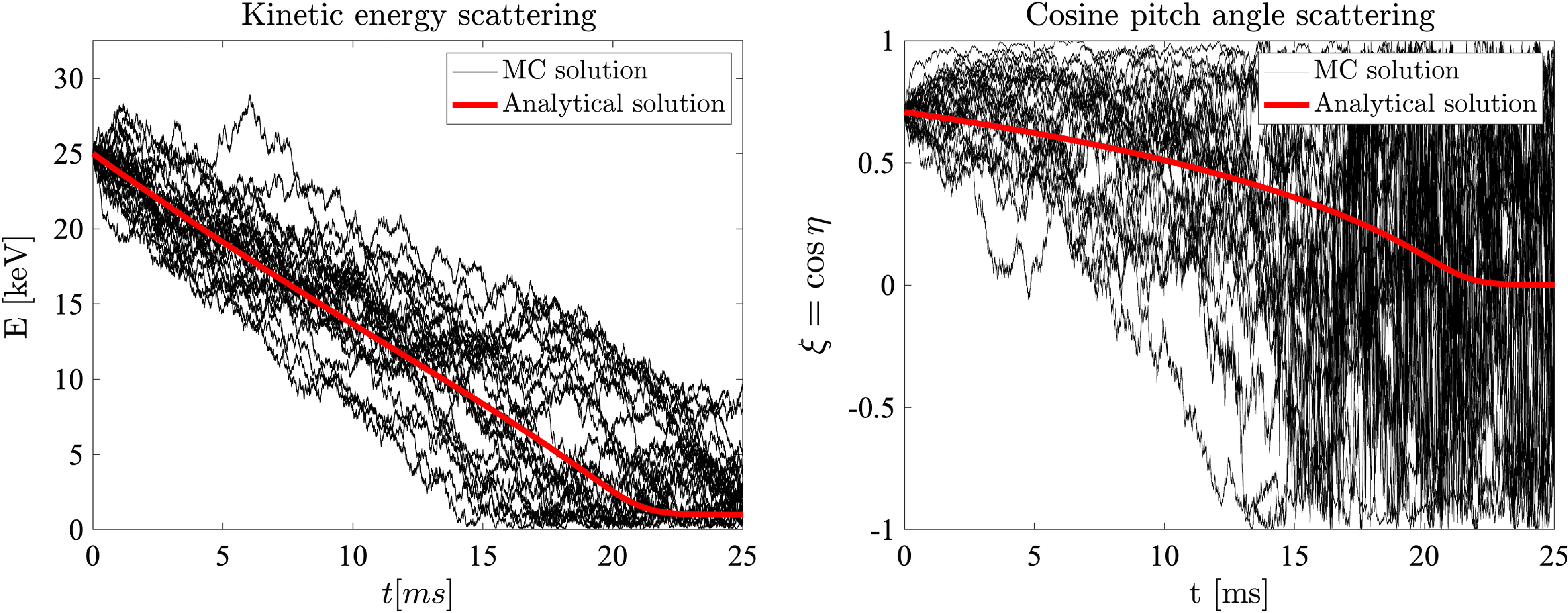
Figure 18. Temporal evolution of the kinetic energy (left) and cosine of pitch angle (right) of a 45 degree 25 keV beam. Monte–Carlo solution with both deterministic and stochastic part presented in black. Analytical solutions presented in red.
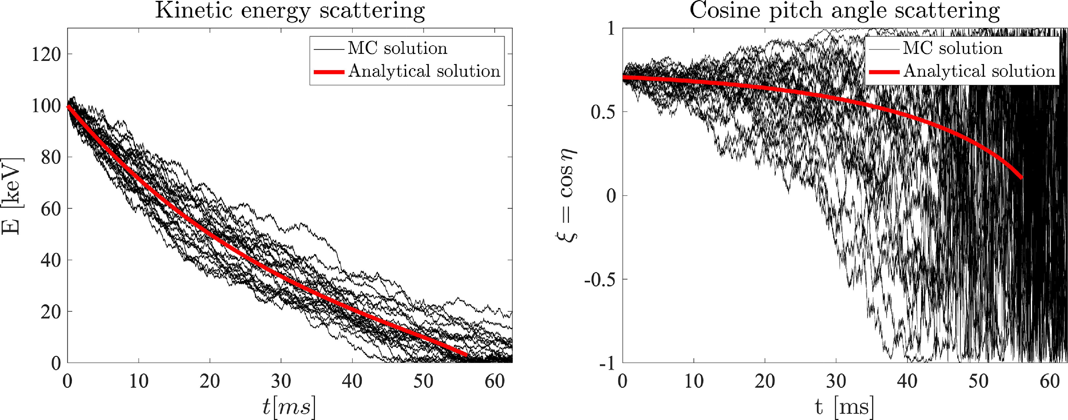
Figure 19. Temporal evolution of the kinetic energy (left) and cosine of pitch angle (right) of a 45 degree 100 keV beam. Monte–Carlo solution with both deterministic and stochastic part presented in black. Analytical solutions presented in red.
Appendix B.
The starting point for deriving the electric field in a quasi-neutral plasma with isotropic but non-uniform profiles is to use equation (2.6). In the case of a uniform electron temperature $T_{e}$
, the electric potential between the central cell and the end-plug takes the form of the so-called Boltzmann relation (B1) where
$T_{e}$
, the electric potential between the central cell and the end-plug takes the form of the so-called Boltzmann relation (B1) where $n_{ep}$
and
$n_{ep}$
and $n_{ec}$
represent the electron density in the end-plug and central cell respectively. Under these circumstances, the potential difference scales linearly with
$n_{ec}$
represent the electron density in the end-plug and central cell respectively. Under these circumstances, the potential difference scales linearly with $T_{e}$
and logarithmically with the ratio of densities.
$T_{e}$
and logarithmically with the ratio of densities.
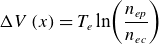 \begin{equation}{\unicode[Arial]{x0394}} V\left(x\right)=T_{e}\ln\! \left(\frac{n_{ep}}{n_{ec}}\right)\end{equation}
What happens when we also have an electron temperature difference ${\unicode[Arial]{x0394}} T_{e}$
between the central cell and end-plug? Can we derive a simple expression to understand the impact of
${\unicode[Arial]{x0394}} T_{e}$
between the central cell and end-plug? Can we derive a simple expression to understand the impact of ${\unicode[Arial]{x0394}} T_{e}$
on the potential? To answer this, we derive a simple expression relating the electron temperature and density to the potential difference by approximating the profiles with Heaviside step functions. This approximation appears to be suitable considering the step-like profiles produced by PICOS++ and presented in figures 1 and 9. The numerical results demonstrate a step-like transition between the central cell and end-plugs.
${\unicode[Arial]{x0394}} T_{e}$
on the potential? To answer this, we derive a simple expression relating the electron temperature and density to the potential difference by approximating the profiles with Heaviside step functions. This approximation appears to be suitable considering the step-like profiles produced by PICOS++ and presented in figures 1 and 9. The numerical results demonstrate a step-like transition between the central cell and end-plugs.
We describe the electron temperature and density profiles with (B2) and (B3) respectively, where $T_{ec}$
represents the electron temperature in the central cell,
$T_{ec}$
represents the electron temperature in the central cell, $T_{ep}$
the electron temperature in the end-plug and
$T_{ep}$
the electron temperature in the end-plug and ${\unicode[Arial]{x0394}} T_{e}=T_{ep}-T_{ec}$
. The term
${\unicode[Arial]{x0394}} T_{e}=T_{ep}-T_{ec}$
. The term $x_{1}$
is the locations where
$x_{1}$
is the locations where $T_{e}$
jumps from
$T_{e}$
jumps from $T_{ec}$
to
$T_{ec}$
to $T_{ep}$
,
$T_{ep}$
, $x_{2}$
where it jumps from
$x_{2}$
where it jumps from $T_{ep}$
to
$T_{ep}$
to $T_{ec}$
and
$T_{ec}$
and $H(x)$
the Heaviside step function.
$H(x)$
the Heaviside step function.
 \begin{equation}T_{e}(x)=T_{ec}+{\unicode[Arial]{x0394}} T_{e}(H(x-x_{1})-H(x-x_{2}))\text{ for }x\gt 0\end{equation}
 \begin{align}n_{e}(x)=n_{ec}+{\unicode[Arial]{x0394}} n_{e}(H(x-x_{1})-H(x-x_{2}))\text{ for }x\gt 0\\[3pt]\nonumber\end{align}
Taking the electron temperature to be isotropic but non-uniform, the parallel electric field is given by (2.6). Integrating the electric field and using integration by parts, the associated potential difference can be written as in (B4). Replacing the electron temperature with the Heaviside approximation (B2), we arrive at the piecewise expression in (B5) where $n_{e}^{*}=n_{e}(x_{1})$
is the electron density at the location where
$n_{e}^{*}=n_{e}(x_{1})$
is the electron density at the location where $T_{e}$
transitions from
$T_{e}$
transitions from $T_{ec}$
to
$T_{ec}$
to $T_{ep}$
. If we broaden the density profile at the transition location, we can approximate
$T_{ep}$
. If we broaden the density profile at the transition location, we can approximate $n_{e}^{*}=n_{e}(x_{1})\approx (n_{ec}+n_{ep})/2$
. Equation (B5) indicates the potential difference scales linearly with the temperature difference
$n_{e}^{*}=n_{e}(x_{1})\approx (n_{ec}+n_{ep})/2$
. Equation (B5) indicates the potential difference scales linearly with the temperature difference ${\unicode[Arial]{x0394}} T_{e}$
and logarithmically with the density. When
${\unicode[Arial]{x0394}} T_{e}$
and logarithmically with the density. When $T_{e}$
becomes uniform, we recover the Boltzmann response for the potential (
$T_{e}$
becomes uniform, we recover the Boltzmann response for the potential ( ${\unicode[Arial]{x0394}} V=T_{e}\ln (n_{ep}/n_{ec})$
).
${\unicode[Arial]{x0394}} V=T_{e}\ln (n_{ep}/n_{ec})$
).
 \begin{equation}{\unicode[Arial]{x0394}} V(x)=\left.T_{e}\right| _{0}^{x}+\left.T_{e}\ln n\right| _{0}^{x}-\int _{0}^{x}\ln n\frac{\partial T_{e}}{\partial s}{\rm d}s\end{equation}
 \begin{align}{\unicode[Arial]{x0394}} V(x)=\left\{\begin{array}{l@{\quad}l} \qquad 0&\text{for }x\lt x_{1}\\ T_{ec}\ln\! \left(\frac{n_{ep}}{n_{ec}}\right)+{\unicode[Arial]{x0394}} T_{e}\left(1+\ln\! \left(\frac{n_{ep}}{n_{e}^{*}}\right)\right); &\text{for }x_{1}\leq x\lt x_{2}\\ \qquad 0&\text{for }x\geq x_{2} \end{array} ;\, n_{e}^{*}\approx \frac{n_{ep}+n_{ec}}{2}\right.\\[-8pt]\nonumber\end{align}


 Open access