


1. Introduction
Let $(x_n)_{n \in \mathbb{N}} \subseteq [0,1]$
be a sequence. The pair correlation counting function of
$(x_n)_{n \in \mathbb{N}} \subseteq [0,1]$
be a sequence. The pair correlation counting function of $(x_n)_{n \in \mathbb{N}} $
is defined by
$(x_n)_{n \in \mathbb{N}} $
is defined by
 \begin{align*} R_2(s,N) = \frac{1}{N}\#\Big\{ 1 \leqslant m \neq n \leqslant N\;:\; \lVert x_m -x_n \rVert \leqslant \frac{s}{N} \Big\}, \qquad s{\gt}0, \end{align*}
where we write $\|x\| = \min\{ |x-k| \;:\; k\in \mathbb{Z} \}$
for the distance of
$\|x\| = \min\{ |x-k| \;:\; k\in \mathbb{Z} \}$
for the distance of $x\in \mathbb{R}$
to its nearest integer. The sequence
$x\in \mathbb{R}$
to its nearest integer. The sequence $(x_n)_{n \in \mathbb{N}} $
is said to have Poissonian pair correlations (or PPC, for abbreviation) if
$(x_n)_{n \in \mathbb{N}} $
is said to have Poissonian pair correlations (or PPC, for abbreviation) if
 \begin{align*}\lim_{N\to \infty}R_2(s,N) = 2s \qquad \text{ for all } s{\gt}0.\end{align*}
The notion of PPC is known to have connections with mathematical physics, which go far beyond the scope of this paper. For instance, we only mention the famous Berry–Tabor Conjecture [Reference Berry and Tabor3]. PPC have recently attracted increasing attention from the purely theoretical point of view. In particular, it has been shown (partially independently) by various authors that sequences with PPC are necessarily uniformly distributed [Reference Aistleitner, Lachmann and Pausinger1, Reference Grepstad and Larcher4, Reference Marklof6, Reference Steinerberger11].
The notion of PPC has an “inhomogeneous” variant, which nonetheless is not equally well studied. Given $\gamma \in \mathbb R,$
we say that a sequence
$\gamma \in \mathbb R,$
we say that a sequence $(x_n)_{n \in \mathbb{N}} $
has
$(x_n)_{n \in \mathbb{N}} $
has $\gamma$
- PPC if
$\gamma$
- PPC if
 \begin{align*}\lim_{N \to \infty} R_2(\gamma;\;s,N) = 2s \qquad \text{ for all }s {\gt} 0, \end{align*}
where we define
 \begin{align*}R_2(\gamma;\;s,N) = \frac{1}{N}\#\Big\{ 1\leqslant m \neq n \leqslant N\;:\; \lVert x_m -x_n - \gamma\rVert \leqslant \frac{s}{N} \Big\}. \end{align*}
Clearly, for $\gamma=0$
and more generally for any integer value of
$\gamma=0$
and more generally for any integer value of $\gamma $
in the above definition, one recovers the classical property of PPC. Since the property of
$\gamma $
in the above definition, one recovers the classical property of PPC. Since the property of $\gamma$
- PPC is invariant under integer translations of
$\gamma$
- PPC is invariant under integer translations of $\gamma,$
we will only consider values of
$\gamma,$
we will only consider values of $\gamma \in [0,1].$
When
$\gamma \in [0,1].$
When $0{\lt} \gamma {\lt} 1$
, we may refer to the property of
$0{\lt} \gamma {\lt} 1$
, we may refer to the property of $\gamma$
- PPC as inhomogeneous Poissonian pair correlations with respect to
$\gamma$
- PPC as inhomogeneous Poissonian pair correlations with respect to $\gamma$
. Also since
$\gamma$
. Also since $\gamma$
- PPC is equivalent to
$\gamma$
- PPC is equivalent to $(1-\gamma)$
- PPC, it will be sufficient to restrict our attention to values
$(1-\gamma)$
- PPC, it will be sufficient to restrict our attention to values $0{\lt} \gamma \leqslant 1/2.$
A first treatment of the notion of $\gamma$
- PPC can be found in [Reference Ramirez7]. There, it is explained that like PPC, the property of
$\gamma$
- PPC can be found in [Reference Ramirez7]. There, it is explained that like PPC, the property of $\gamma$
- PPC with
$\gamma$
- PPC with $\gamma\neq 0$
is a pseudorandomness property, in the sense that if
$\gamma\neq 0$
is a pseudorandomness property, in the sense that if $(X_n)_{n=1}^{\infty}$
is a sequence of i.i.d. random variables, all following the uniform distribution in [0, 1], then with probability 1 the sequence
$(X_n)_{n=1}^{\infty}$
is a sequence of i.i.d. random variables, all following the uniform distribution in [0, 1], then with probability 1 the sequence $(X_n)_{n=1}^{\infty}$
has
$(X_n)_{n=1}^{\infty}$
has $\gamma$
- PPC. In [Reference Ramirez7] it is also stated among other results that just like their homogeneous counterpart,
$\gamma$
- PPC. In [Reference Ramirez7] it is also stated among other results that just like their homogeneous counterpart, $\gamma$
- PPC is a property that is stronger than uniform distribution; in other words, any sequence with
$\gamma$
- PPC is a property that is stronger than uniform distribution; in other words, any sequence with $\gamma$
- PPC is automatically uniformly distributed.
$\gamma$
- PPC is automatically uniformly distributed.
In the first result of our paper, we prove that this statement is actually false!
Theorem 1·1. Let $0{\lt}\gamma {\lt}1$
. Then there exists a sequence
$0{\lt}\gamma {\lt}1$
. Then there exists a sequence $(x_n)_{n \in \mathbb{N}} \subseteq [0,1]$
that has
$(x_n)_{n \in \mathbb{N}} \subseteq [0,1]$
that has $\gamma$
- PPC but is not uniformly distributed.
$\gamma$
- PPC but is not uniformly distributed.
In addition to Theorem 1·1, we try to shed some light on the reason why PPC imply uniform distribution while $\gamma$
- PPC with
$\gamma$
- PPC with $\gamma\neq 0$
do not. Among the several proofs of the fact that PPC imply uniform distribution that were mentioned earlier, Aistleitner, Lachmann and Pausinger in [Reference Aistleitner, Lachmann and Pausinger1] prove a stronger statement that connects the limiting behaviour of the pair correlation function
$\gamma\neq 0$
do not. Among the several proofs of the fact that PPC imply uniform distribution that were mentioned earlier, Aistleitner, Lachmann and Pausinger in [Reference Aistleitner, Lachmann and Pausinger1] prove a stronger statement that connects the limiting behaviour of the pair correlation function $R_2(s,N)$
with the asymptotic distribution function of the sequence
$R_2(s,N)$
with the asymptotic distribution function of the sequence $(x_n)_{n \in \mathbb{N}} .$
We say that the function
$(x_n)_{n \in \mathbb{N}} .$
We say that the function $G:[0,1] \to \mathbb{R}$
is the asymptotic distribution function of the sequence
$G:[0,1] \to \mathbb{R}$
is the asymptotic distribution function of the sequence $(x_n)_{n \in \mathbb{N}} $
if
$(x_n)_{n \in \mathbb{N}} $
if
 \begin{align*} G(x) = \lim_{N\to \infty} \frac{1}{N}\#\{ n\leqslant N \;:\; 0 \leqslant x_n \leqslant x\} \qquad \text{ for all } 0 \leqslant x \leqslant 1. \end{align*}
Their result is the following.
Theorem (ALP). Let $(x_n)_{n \in \mathbb{N}} \subseteq [0,1]$
be a sequence with asymptotic distribution function
$(x_n)_{n \in \mathbb{N}} \subseteq [0,1]$
be a sequence with asymptotic distribution function $G:[0,1] \to \mathbb{R}.$
Let
$G:[0,1] \to \mathbb{R}.$
Let $F:[0,\infty)\rightarrow [0,\infty]$
be defined by
$F:[0,\infty)\rightarrow [0,\infty]$
be defined by
 \begin{align*} F(s) = \liminf_{N \to \infty}\frac{1}{N} \# \Big\{1 \leqslant m\neq n \leqslant N \;:\; \|x_m - x_n \| \leqslant \frac{s}{N} \Big\}, \qquad s{\gt}0. \end{align*}
Then the following hold:
-
(i) if G is not absolutely continuous, then $F(s)=\infty$
for all
$s{\gt}0$
;
$F(s)=\infty$
for all
$s{\gt}0$
; -
(ii) if G is absolutely continuous and g is the corresponding density function (that is,
$g = G'$
almost everywhere), then (1·1)
\begin{equation} \limsup_{s \to \infty}\frac{F(s)}{2s} \geqslant \int_0^1 g(x)^2 \,\mathrm{d}x. \end{equation}


This resultFootnote
1
indeed implies that PPC is a property stronger than uniform distribution. If $(x_n)_{n \in \mathbb{N}} $
is not u.d. mod 1, then the integral on the right-hand side of (1·1) is strictly greater than 1 and
$(x_n)_{n \in \mathbb{N}} $
is not u.d. mod 1, then the integral on the right-hand side of (1·1) is strictly greater than 1 and $(x_n)_{n \in \mathbb{N}} $
cannot have PPC.
$(x_n)_{n \in \mathbb{N}} $
cannot have PPC.
For uniformly distributed sequences, the density function is $g(x)=1$
and thus the ALP Theorem implies that for any
$g(x)=1$
and thus the ALP Theorem implies that for any $\varepsilon {\gt} 0$
,
$\varepsilon {\gt} 0$
, $\liminf_{N\to \infty}R_2(s,N) \geqslant 2s- \varepsilon$
for arbitrarily large values of the scale
$\liminf_{N\to \infty}R_2(s,N) \geqslant 2s- \varepsilon$
for arbitrarily large values of the scale $s{\gt}0.$
In other words, among all uniformly distributed sequences, for those who have PPC, the quantity
$s{\gt}0.$
In other words, among all uniformly distributed sequences, for those who have PPC, the quantity
 \begin{align*}\limsup_{s \to \infty}\liminf_{N\to\infty}\frac{R_2(s,N)}{2s}\end{align*}
exhibits an extremal behaviour, in the sense that it has the minimal possible asymptotic size, and this extremal behaviour is not attainable for non-uniformly distributed sequences.
Returning to the inhomogeneous PPC, the proof of Theorem 1·1 makes use of the following statement, which establishes a connection between the density function g and the limiting behaviour of $R_2(\gamma;\;s,N)$
in a probabilistic context. We say that a random variable X with support in [0, 1] is distributed with respect to the function
$R_2(\gamma;\;s,N)$
in a probabilistic context. We say that a random variable X with support in [0, 1] is distributed with respect to the function $G\;:\;[0,1]\to \mathbb{R}$
if
$G\;:\;[0,1]\to \mathbb{R}$
if $\mathbb P(X{\lt} t) = G(t)$
for all
$\mathbb P(X{\lt} t) = G(t)$
for all $t\in [0,1].$
Theorem 1·2. Let $\gamma\in\mathbb R$
and
$\gamma\in\mathbb R$
and $G:[0,1]\to \mathbb{R}$
be an absolutely continuous distribution function with corresponding density function
$G:[0,1]\to \mathbb{R}$
be an absolutely continuous distribution function with corresponding density function $g\in L^2([0,1]).$
Let
$g\in L^2([0,1]).$
Let $(X_n)_{n\in\mathbb N}$
be a sequence of independent random variables on some probability space
$(X_n)_{n\in\mathbb N}$
be a sequence of independent random variables on some probability space $(\Omega, \Sigma, \mathbb P)$
with support in [0, 1] that are distributed with respect to G. Then, for the
$(\Omega, \Sigma, \mathbb P)$
with support in [0, 1] that are distributed with respect to G. Then, for the $\gamma$
-pair correlation function of
$\gamma$
-pair correlation function of $(x_n)_{n\in\mathbb N} \;:\!=\; {}(X_n(\omega))_{n\in\mathbb N}, \omega \in \Omega$
, we have
$(x_n)_{n\in\mathbb N} \;:\!=\; {}(X_n(\omega))_{n\in\mathbb N}, \omega \in \Omega$
, we have $\mathbb{P}$
-almost surely
$\mathbb{P}$
-almost surely
 \begin{equation} {} {}\lim_{N\to \infty} R_2(\gamma;\;s,N) = 2s \cdot \int_{0}^{1} g(x)g(x + \gamma)\,\mathrm{d}x \qquad \text{ for all } s{\gt}0. {}\end{equation}
Remark 1·3. In the rest of the paper, when $g:[0,1]\to \mathbb{R}$
is a density function as above and
$g:[0,1]\to \mathbb{R}$
is a density function as above and $\gamma\neq 0,$
we implicitly extend g to the real numbers periodically mod 1 and write
$\gamma\neq 0,$
we implicitly extend g to the real numbers periodically mod 1 and write $\int_0^1 g(x)g(x+\gamma)\,\mathrm{d} x$
instead of
$\int_0^1 g(x)g(x+\gamma)\,\mathrm{d} x$
instead of $\int_0^1 g(x)g(\{x+\gamma\})\,\mathrm{d} x$
, which would be more accurate.
$\int_0^1 g(x)g(\{x+\gamma\})\,\mathrm{d} x$
, which would be more accurate.
We note that for the specific choice $\gamma=0,$
Theorem 1·2 is the heuristic observation made in [Reference Aistleitner, Lachmann and Pausinger1, equation (2)]. Theorem 1·1 follows straightforwardly from Theorem 1·2 once we find a non-constant density g such that
$\gamma=0,$
Theorem 1·2 is the heuristic observation made in [Reference Aistleitner, Lachmann and Pausinger1, equation (2)]. Theorem 1·1 follows straightforwardly from Theorem 1·2 once we find a non-constant density g such that $\int_{0}^{1} g(x)g(x + \gamma)\,\mathrm{d}x = 1$
for a fixed
$\int_{0}^{1} g(x)g(x + \gamma)\,\mathrm{d}x = 1$
for a fixed $\gamma$
.
$\gamma$
.
After establishing the connection between $R_2(\gamma;\;s,N)$
and the density function g for random variables described in (1·2), we suspected that an analogue of the ALP Theorem is also true for
$R_2(\gamma;\;s,N)$
and the density function g for random variables described in (1·2), we suspected that an analogue of the ALP Theorem is also true for $\gamma\neq 0.$
That is, if g is the distribution function of the sequence
$\gamma\neq 0.$
That is, if g is the distribution function of the sequence $(x_n)_{n \in \mathbb{N}} $
and we define
$(x_n)_{n \in \mathbb{N}} $
and we define
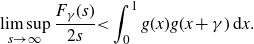
 \begin{equation} F_\gamma(s) = \liminf_{N \to \infty}\frac{1}{N} \# \Big\{ 1\leqslant m\neq n \leqslant N \;:\; \|x_m - x_n -\gamma \| \leqslant \frac{s}{N} \Big\}, \qquad s{\gt}0, \end{equation}
then
 \begin{equation} \limsup_{s \to \infty}\frac{F_\gamma(s)}{2s} \geqslant \int_0^1 g(x)g(x+\gamma)\,\mathrm{d}x. \end{equation}
However, it turns out that (1.4) is not true, either.
Theorem 1·4. For any $0{\lt}\gamma {\lt}1$
, there exists a sequence
$0{\lt}\gamma {\lt}1$
, there exists a sequence $(x_n)_{n \in \mathbb{N}} \subseteq [0,1]$
with asymptotic density function
$(x_n)_{n \in \mathbb{N}} \subseteq [0,1]$
with asymptotic density function $g\;:\; [0,1] \to \mathbb{R}$
such that for the function
$g\;:\; [0,1] \to \mathbb{R}$
such that for the function $F_\gamma$
as in (1.3) we have
$F_\gamma$
as in (1.3) we have
 \begin{align*} \limsup_{s\to \infty} \frac{F_\gamma(s)}{2s} {\lt} \int_0^1 g(x)g(x+\gamma)\,\mathrm{d}x. \end{align*}
Finally, we examine the relation between the property of $\gamma$
- PPC for different values of
$\gamma$
- PPC for different values of $\gamma.$
Observe that in view of Theorem 1·1,
$\gamma.$
Observe that in view of Theorem 1·1, $\gamma$
- PPC for
$\gamma$
- PPC for $\gamma \neq 0$
does not imply PPC; otherwise, every sequence with
$\gamma \neq 0$
does not imply PPC; otherwise, every sequence with $\gamma$
- PPC would need to be uniformly distributed. As a last result of the paper, we show that this is not a phenomenon that distinguishes between PPC and inhomogeneous pair correlations. In particular, it follows that the classical PPC property is not stronger than its inhomogeneous counterparts.
$\gamma$
- PPC would need to be uniformly distributed. As a last result of the paper, we show that this is not a phenomenon that distinguishes between PPC and inhomogeneous pair correlations. In particular, it follows that the classical PPC property is not stronger than its inhomogeneous counterparts.
Theorem 1·5. Let $\gamma_1,\gamma_2 \in [0,1/2]$
with
$\gamma_1,\gamma_2 \in [0,1/2]$
with $\gamma_1 \neq \gamma_2$
. Then there exists a sequence
$\gamma_1 \neq \gamma_2$
. Then there exists a sequence $(x_n)_{n \in \mathbb{N}} \subseteq [0,1]$
that has
$(x_n)_{n \in \mathbb{N}} \subseteq [0,1]$
that has $\gamma_1$
- PPC but not
$\gamma_1$
- PPC but not $\gamma_2$
- PPC.
$\gamma_2$
- PPC.
Why $\gamma$
- PPC? Before proceeding to the proofs of the theorems, we think it would be worth discussing what we view as the motivation behind the definition of
$\gamma$
- PPC? Before proceeding to the proofs of the theorems, we think it would be worth discussing what we view as the motivation behind the definition of $\gamma$
- PPC. Beyond pure interest in the notion itself, this motivation arises in an open problem from the metric theory of (homogeneous) Poissonian pair correlations. Given an increasing sequence
$\gamma$
- PPC. Beyond pure interest in the notion itself, this motivation arises in an open problem from the metric theory of (homogeneous) Poissonian pair correlations. Given an increasing sequence $\mathcal{A} = (a_n)_{n\in \mathbb N} \subseteq \mathbb N$
, a series of results [Reference Aistleitner, Larcher and Lewko2, Reference Rudnick and Sarnak8–Reference Rudnick and Zaharescu10] shows that under certain assumptions on
$\mathcal{A} = (a_n)_{n\in \mathbb N} \subseteq \mathbb N$
, a series of results [Reference Aistleitner, Larcher and Lewko2, Reference Rudnick and Sarnak8–Reference Rudnick and Zaharescu10] shows that under certain assumptions on $\mathcal{A}$
, the sequence
$\mathcal{A}$
, the sequence $(a_nx)_{n\in \mathbb N} $
has PPC for almost all
$(a_nx)_{n\in \mathbb N} $
has PPC for almost all $x\in [0,1]$
. There also exist results [Reference Aistleitner, Larcher and Lewko2, 12] that provide conditions on
$x\in [0,1]$
. There also exist results [Reference Aistleitner, Larcher and Lewko2, 12] that provide conditions on $\mathcal{A}$
under which the sequence
$\mathcal{A}$
under which the sequence $(a_n x)_{n\in \mathbb N}$
has PPC for almost no
$(a_n x)_{n\in \mathbb N}$
has PPC for almost no $x\in [0,1].$
However, it remains an open question to determine whether for any choice of
$x\in [0,1].$
However, it remains an open question to determine whether for any choice of $\mathcal{A}$
, the sequence
$\mathcal{A}$
, the sequence $(a_n x)_{n\in \mathbb N}$
has PPC either for almost all or for almost no
$(a_n x)_{n\in \mathbb N}$
has PPC either for almost all or for almost no $x\in [0,1],$
thus establishing a zero-one law in the theory of metric Poissonian pair correlations.
$x\in [0,1],$
thus establishing a zero-one law in the theory of metric Poissonian pair correlations.
For $\mathcal{A}$
fixed, writing
$\mathcal{A}$
fixed, writing $ X_{\mathcal{A}} = \{ x\in [0,1] \;:\; (a_nx)_{n\in\mathbb N} \text{ has PPC}\},$
the aforementioned problem is equivalent to determining whether
$ X_{\mathcal{A}} = \{ x\in [0,1] \;:\; (a_nx)_{n\in\mathbb N} \text{ has PPC}\},$
the aforementioned problem is equivalent to determining whether $\lambda(X_{\mathcal{A}})=0$
or 1 for any choice of
$\lambda(X_{\mathcal{A}})=0$
or 1 for any choice of $\mathcal{A}.$
To answer this question, it would suffice to check whether the set
$\mathcal{A}.$
To answer this question, it would suffice to check whether the set $X_\mathcal{A}$
is invariant under the ergodic transformation
$X_\mathcal{A}$
is invariant under the ergodic transformation $T(x) = 2x \mod 1.$
Given
$T(x) = 2x \mod 1.$
Given $x\in X_\mathcal{A},$
we have
$x\in X_\mathcal{A},$
we have $2x\in X_\mathcal{A}$
if and only if the pair correlation function of the sequence
$2x\in X_\mathcal{A}$
if and only if the pair correlation function of the sequence $(2a_nx)_{n\in\mathbb N}$
satisfies
$(2a_nx)_{n\in\mathbb N}$
satisfies $\lim_{N\to \infty}R_2(2x,2s,N) = 4s$
for all
$\lim_{N\to \infty}R_2(2x,2s,N) = 4s$
for all $s{\gt}0$
. But
$s{\gt}0$
. But
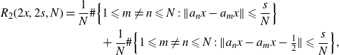 \begin{align*} R_2(2x,2s,N) &= \frac{1}{N}\#\Big\{ 1\leqslant m\neq n \leqslant N \;:\; \|a_nx-a_mx\| \leqslant \frac{s}{N}\Big\} \\ & \qquad \quad +\frac{1}{N}\#\Big\{ 1\leqslant m\neq n \leqslant N \;:\; \|a_nx-a_mx-\tfrac12 \| \leqslant \frac{s}{N}\Big\}, \end{align*}
and therefore $2x\in X_\mathcal{A}$
if and only if the sequence
$2x\in X_\mathcal{A}$
if and only if the sequence $(a_nx)_{n\in\mathbb N}$
has
$(a_nx)_{n\in\mathbb N}$
has ${1}/{2}$
-PPC! In particular, Theorem 1·4 shows that the naïvest approach of immediately implying
${1}/{2}$
-PPC! In particular, Theorem 1·4 shows that the naïvest approach of immediately implying $2x \in X_{\mathcal{A}}$
does not work and thus, if possible at all, one has to use the additional structure of the sequence.
$2x \in X_{\mathcal{A}}$
does not work and thus, if possible at all, one has to use the additional structure of the sequence.
Notation. Given $x\in \mathbb{R}$
and
$x\in \mathbb{R}$
and $r{\gt}0$
we write
$r{\gt}0$
we write $B(x,r)=\{ t \in \mathbb{R} \;:\; \|t-x\| \leqslant r\}$
for the interval of points in the unit torus that have distance at most r from x. Also throughout the text we shall use the standard Vinogradov
$B(x,r)=\{ t \in \mathbb{R} \;:\; \|t-x\| \leqslant r\}$
for the interval of points in the unit torus that have distance at most r from x. Also throughout the text we shall use the standard Vinogradov $\ll$
-notation: we write
$\ll$
-notation: we write $f(x)\ll g(x), x\to \infty$
when
$f(x)\ll g(x), x\to \infty$
when $\limsup_{x\to \infty} f(x)/g(x) {\lt} \infty$
.
$\limsup_{x\to \infty} f(x)/g(x) {\lt} \infty$
.
2. Proof of Theorems 1·1 and 1·2
As explained in the introduction, we begin with the proof of Theorem 1·2, which is a more general result of probabilistic nature. The existence of sequences $(x_n)_{n \in \mathbb{N}} $
with
$(x_n)_{n \in \mathbb{N}} $
with $\gamma$
–PPC that are not uniformly distributed will then follow as a simple corollary.
$\gamma$
–PPC that are not uniformly distributed will then follow as a simple corollary.
2·1. Proof of Theorem 1·2
When $m\neq n,$
the random variable
$m\neq n,$
the random variable $X_m - X_n$
has probability density function
$X_m - X_n$
has probability density function
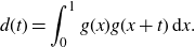 \begin{align} {}d(t) & = \int_0^1 g(x)g(x+t)\,\mathrm{d} x.\end{align}
Writing $\mathcal{X} \;:\!=\; (X_n)_{n \in \mathbb{N}}$
, the
$\mathcal{X} \;:\!=\; (X_n)_{n \in \mathbb{N}}$
, the $\gamma$
-pair correlation function
$\gamma$
-pair correlation function
 \begin{align*} R_2^{\mathcal{X}}(\gamma;\; s, N ) \;:\!=\; \frac{1}{N}\sum_{m\neq n\leqslant N}{\unicode[Times]{x1D7D9}}_{B(0,\frac{s}{N})}(X_m-X_n-\gamma) = \frac{1}{N}\sum_{m\neq n\leqslant N} {\unicode[Times]{x1D7D9}}_{B(\gamma,\frac{s}{N})}(X_m-X_n) \end{align*}
is itself a random variable with expectation
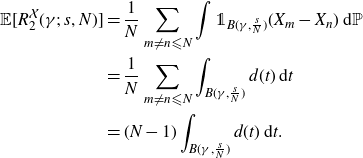 \begin{align*} {}\mathbb E[R_2^{\mathcal{X}}(\gamma;\; s, N ) ] &= \frac{1}{N}\sum_{m\neq n \leqslant N}\int {\unicode[Times]{x1D7D9}}_{B(\gamma,\frac{s}{N}) }(X_m-X_n)\,\mathrm{d} \mathbb P \\ & = \frac{1}{N} \sum_{m\neq n \leqslant N}\int_{B(\gamma,\frac{s}{N}) } d(t)\,\mathrm{d} t \\ &= (N-1)\int_{B(\gamma,\frac{s}{N}) }d(t) \,\mathrm{d} t.\end{align*}
Since $g\in L^2([0,1]),$
the function d(t) defined in (2·1) is bounded and continuous, hence
$g\in L^2([0,1]),$
the function d(t) defined in (2·1) is bounded and continuous, hence
 \begin{align*} \lim_{N\to\infty}N \int_{B(\gamma,\frac{s}{N}) } d(t)\,\mathrm{d} t = \lim_{N\to \infty}2s\cdot \frac{1}{2s/N} \int_{B(\gamma,\frac{s}{N}) }d(t)\,\mathrm{d} t = 2s\cdot d(\gamma). \end{align*}
This allows us to conclude that
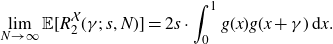 \begin{align*} \lim_{N\to \infty}\mathbb E[R_2^{\mathcal{X}}(\gamma;\; s, N )] = 2s \cdot \int_{0}^{1} g(x)g(x + \gamma) \,\mathrm{d}x. \end{align*}
In the rest of the proof, we will write
 \begin{align*} \mathcal{D}_N = \{ (m,n)\in \mathbb N^2 \;:\; 1\leqslant m \neq n \leqslant N\} \end{align*}
for the set of pairs of indices appearing in the pair correlation functions.
The second moment of $R_2^{\mathcal{X}}(\gamma;\; s, N )$
is equal to
$R_2^{\mathcal{X}}(\gamma;\; s, N )$
is equal to
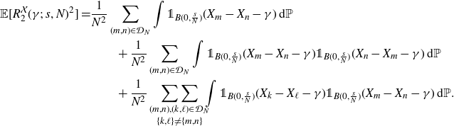 \begin{equation} {}\begin{split} \mathbb E[ R_2^{\mathcal{X}}(\gamma;\; s, N )^2] = &\frac{1}{N^2}\sum_{(m,n) \in \mathcal{D}_N }\int {\unicode[Times]{x1D7D9}}_{B(0,\frac{s}{N})}(X_m-X_n-\gamma) \,\mathrm{d} \mathbb P \qquad \qquad \qquad \qquad \\ {} {}\qquad &\qquad + \frac{1}{N^2}\sum_{(m,n) \in \mathcal{D}_N }\int {\unicode[Times]{x1D7D9}}_{B(0,\frac{s}{N})}(X_m-X_n-\gamma) {\unicode[Times]{x1D7D9}}_{B(0,\frac{s}{N})}(X_n-X_m-\gamma)\,\mathrm{d} \mathbb P \qquad \qquad \qquad \qquad \\ {} {}\qquad &\qquad + \frac{1}{N^2}\mathop{\mathop{\sum\sum}_{(m,n), (k,\ell) \in \mathcal{D}_N}}_{ \{k,\ell\} \neq \{m,n\}} \hspace{-2mm} \int {\unicode[Times]{x1D7D9}}_{B(0,\frac{s}{N}) }(X_k-X_\ell-\gamma){\unicode[Times]{x1D7D9}}_{ B(0,\frac{s}{N})}(X_m-X_n-\gamma) \,\mathrm{d} \mathbb P. \end{split}\end{equation}
The first of the terms above is equal to $({1}/{N}) \mathbb E[ R_2(\gamma;\;s,N)].$
For the second term, we note that for
$({1}/{N}) \mathbb E[ R_2(\gamma;\;s,N)].$
For the second term, we note that for $\gamma = 0$
or
$\gamma = 0$
or $\gamma = 1/2$
, we get another contribution of
$\gamma = 1/2$
, we get another contribution of $({1}/{N}) \mathbb E[ R_2(\gamma;\;s,N)]$
, while if
$({1}/{N}) \mathbb E[ R_2(\gamma;\;s,N)]$
, while if $\gamma \notin \{0,1/2\}$
, the second term vanishes for N sufficiently large. Thus, in any case, the contribution of the second term is bounded from above by
$\gamma \notin \{0,1/2\}$
, the second term vanishes for N sufficiently large. Thus, in any case, the contribution of the second term is bounded from above by $({1}/{N}) \mathbb E[ R_2(\gamma;\;s,N)]$
, and it remains to examine the third term of (2·2).
$({1}/{N}) \mathbb E[ R_2(\gamma;\;s,N)]$
, and it remains to examine the third term of (2·2).
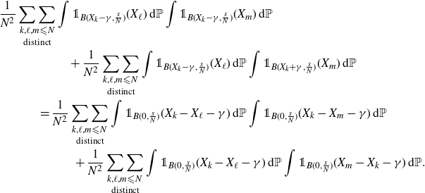
In order to do so, note that the contribution of pairs $(k,\ell), (m,n) \in \mathcal{D}_N$
that share one common coordinate is
$(k,\ell), (m,n) \in \mathcal{D}_N$
that share one common coordinate is
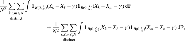 \begin{multline*} {}\frac{1}{N^2}\mathop{\mathop{\sum\sum}_{k,\ell,m \leqslant N}}_{\text{distinct}} \int {\unicode[Times]{x1D7D9}}_{B(0,\frac{s}{N})}(X_k-X_\ell-\gamma) {\unicode[Times]{x1D7D9}}_{B(0,\frac{s}{N})}(X_k-X_m-\gamma) \,\mathrm{d} \mathbb P \quad \\ + \frac{1}{N^2}\mathop{\mathop{\sum\sum}_{k,\ell,m \leqslant N}}_{\text{distinct}} \int {\unicode[Times]{x1D7D9}}_{B(0,\frac{s}{N})}(X_k-X_\ell-\gamma) {\unicode[Times]{x1D7D9}}_{B(0,\frac{s}{N})}(X_m-X_k-\gamma) \,\mathrm{d} \mathbb P,\end{multline*}
which is equal to
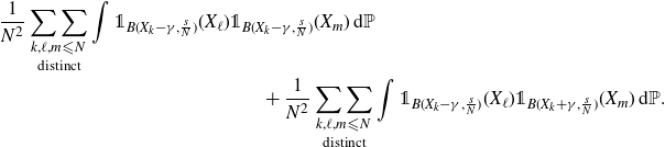 \begin{multline*} {}\frac{1}{N^2}\mathop{\mathop{\sum\sum}_{k,\ell,m \leqslant N}}_{ \text{distinct}} \int {\unicode[Times]{x1D7D9}}_{B(X_k-\gamma,\frac{s}{N})}(X_\ell) {\unicode[Times]{x1D7D9}}_{B(X_k-\gamma,\frac{s}{N})}(X_m) \,\mathrm{d} \mathbb P \quad \\ + \frac{1}{N^2}\mathop{\mathop{\sum\sum}_{k,\ell,m \leqslant N}}_{\text{distinct}} \int {\unicode[Times]{x1D7D9}}_{B(X_k-\gamma,\frac{s}{N})}(X_\ell) {\unicode[Times]{x1D7D9}}_{B(X_k+\gamma,\frac{s}{N})}(X_m) \,\mathrm{d} \mathbb P.\end{multline*}
Since for $\ell \neq m$
the random variables
$\ell \neq m$
the random variables $X_\ell, X_m$
are independent, the above is equal to
$X_\ell, X_m$
are independent, the above is equal to
 \begin{multline*} {}\frac{1}{N^2}\mathop{\mathop{\sum\sum}_{k,\ell,m \leqslant N}}_{ \text{distinct}} \int {\unicode[Times]{x1D7D9}}_{B(X_k-\gamma,\frac{s}{N})}(X_\ell)\,\mathrm{d}\mathbb P \int {\unicode[Times]{x1D7D9}}_{B(X_k-\gamma,\frac{s}{N})}(X_m) \,\mathrm{d} \mathbb P \quad \\ + \frac{1}{N^2}\mathop{\mathop{\sum\sum}_{k,\ell,m \leqslant N}}_{\text{distinct}} \int {\unicode[Times]{x1D7D9}}_{B(X_k-\gamma,\frac{s}{N})}(X_\ell) \,\mathrm{d} \mathbb P \int {\unicode[Times]{x1D7D9}}_{B(X_k+\gamma,\frac{s}{N})}(X_m) \,\mathrm{d} \mathbb P \\ = \frac{1}{N^2}\mathop{\mathop{\sum\sum}_{k,\ell,m \leqslant N}}_{\text{distinct}} \int {\unicode[Times]{x1D7D9}}_{B(0,\frac{s}{N})}(X_k-X_\ell-\gamma) \,\mathrm{d}\mathbb P \int {\unicode[Times]{x1D7D9}}_{B(0,\frac{s}{N})}(X_k-X_m-\gamma) \,\mathrm{d} \mathbb P \\ + \frac{1}{N^2}\mathop{\mathop{\sum\sum}_{k,\ell,m \leqslant N}}_{\text{distinct}} \int {\unicode[Times]{x1D7D9}}_{B(0,\frac{s}{N})}(X_k-X_\ell-\gamma)\,\mathrm{d}\mathbb P \int {\unicode[Times]{x1D7D9}}_{B(0,\frac{s}{N})}(X_m-X_k-\gamma) \,\mathrm{d} \mathbb P.\end{multline*}
Back to (2·2), for pairs $(k,\ell), (m,n) \in \mathcal{D}_N$
with no common coordinate, the random variables
$(k,\ell), (m,n) \in \mathcal{D}_N$
with no common coordinate, the random variables $X_k-X_\ell$
,
$X_k-X_\ell$
, $X_m-X_n$
are independent and the corresponding contribution is
$X_m-X_n$
are independent and the corresponding contribution is
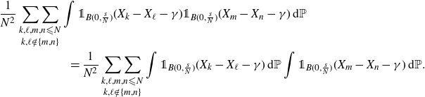 \begin{multline*} {}\frac{1}{N^2}\mathop{\mathop{\sum\sum}_{k,\ell,m,n\leqslant N}}_{k,\ell \notin \{m,n\}}\int {\unicode[Times]{x1D7D9}}_{B(0,\frac{s}{N})}(X_k-X_\ell-\gamma){\unicode[Times]{x1D7D9}}_{B(0,\frac{s}{N})}(X_m-X_n-\gamma)\,\mathrm{d}\mathbb P \\ = \frac{1}{N^2}\mathop{\mathop{\sum\sum}_{k,\ell,m,n\leqslant N}}_{k,\ell \notin \{m,n\}}\int {\unicode[Times]{x1D7D9}}_{B(0,\frac{s}{N})}(X_k-X_\ell-\gamma)\,\mathrm{d} \mathbb P \int {\unicode[Times]{x1D7D9}}_{B(0,\frac{s}{N})}(X_m-X_n-\gamma)\,\mathrm{d}\mathbb P.\end{multline*}
If we apply the same case distinction to the sum in
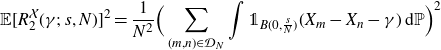 \begin{align*} {}\mathbb E[ R_2^{\mathcal{X}}(\gamma;\; s, N )]^2 &= \frac{1}{N^2}\Big( \sum_{(m,n)\in \mathcal{D}_N} \int {\unicode[Times]{x1D7D9}}_{B(0,\frac{s}{N})}(X_m-X_n-\gamma)\,\mathrm{d} \mathbb P \Big)^2\end{align*}
and combine with the equations above, we deduce that
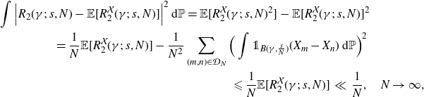 \begin{multline*} {}\int \Big| R_2(\gamma;\;s,N) - \mathbb E[ R_2^{\mathcal{X}}(\gamma;\; s, N ) ] \Big|^2 \,\mathrm{d} \mathbb P = \mathbb E[ R_2^{\mathcal{X}}(\gamma;\; s, N )^2 ] - \mathbb E[ R_2^{\mathcal{X}}(\gamma;\; s, N ) ]^2 \\ {}= \frac{1}{N}\mathbb E[ R_2^{\mathcal{X}}(\gamma;\; s, N )] - \frac{1}{N^2}\sum_{(m,n)\in \mathcal{D}_N}\Big( \int {\unicode[Times]{x1D7D9}}_{B(\gamma,\frac{s}{N})}(X_m-X_n)\,\mathrm{d}\mathbb P\Big)^2 \\ \leqslant \frac{1}{N}\mathbb E[ R_2^{\mathcal{X}}(\gamma;\; s, N ) ] \, \ll \, \frac{1}{N}, \quad N\to \infty,\end{multline*}
where we used again that $g \in L^2([0,1])$
. An application of Chebyshev’s inequality in combination with the first Borel–Cantelli Lemma shows that
$g \in L^2([0,1])$
. An application of Chebyshev’s inequality in combination with the first Borel–Cantelli Lemma shows that $\mathbb{P}$
-almost surely in
$\mathbb{P}$
-almost surely in $\omega\in \Omega$
we have
$\omega\in \Omega$
we have
 \begin{align*} \lim_{N\to \infty} R_2^{\mathcal{X}(\omega)}(\gamma;\; s, N^2) = \lim_{N\to \infty} \mathbb E[ R_2^{\mathcal{X}}(\gamma;\; s, N^2)] = 2s \cdot \int_{0}^{1} g(x)g(x + \gamma) \,\mathrm{d}x,\end{align*}
and a standard approximation argument (see e.g. [Reference Aistleitner, Larcher and Lewko2, p. 475]) shows that the same is true along the whole sequence $R_2(\gamma;\;s,N)$
. This proves (1·2) for fixed
$R_2(\gamma;\;s,N)$
. This proves (1·2) for fixed $s {\gt} 0$
.
$s {\gt} 0$
.
In order to deduce (1·2) for all $s {\gt} 0$
simultaneously, we apply the above procedure for every
$s {\gt} 0$
simultaneously, we apply the above procedure for every $s \in \mathbb{Q}_{\geqslant 0}$
. Using that
$s \in \mathbb{Q}_{\geqslant 0}$
. Using that $\mathbb{Q}$
is countable and dense in
$\mathbb{Q}$
is countable and dense in $\mathbb{R}$
, the monotonicity of
$\mathbb{R}$
, the monotonicity of $R_2(\gamma;\;s,N)$
as a function in s, and the continuity of
$R_2(\gamma;\;s,N)$
as a function in s, and the continuity of $s \mapsto 2s \cdot \int_{0}^{1} g(x)g(x + \gamma)\,\mathrm{d}x$
allows us to deduce that (1·2) holds almost surely for all
$s \mapsto 2s \cdot \int_{0}^{1} g(x)g(x + \gamma)\,\mathrm{d}x$
allows us to deduce that (1·2) holds almost surely for all $s {\gt}0$
.
$s {\gt}0$
.
2·2. Proof of Theorem 1·1
In view of Theorem 1·2, in order to prove the existence of a sequence with $\gamma$
- PPC that is not uniformly distributed, it simply suffices to define a density function g such that
$\gamma$
- PPC that is not uniformly distributed, it simply suffices to define a density function g such that $\int_0^1 g(x)g(x+\gamma)\,\mathrm{d} x =1$
and g is not identically equal to
$\int_0^1 g(x)g(x+\gamma)\,\mathrm{d} x =1$
and g is not identically equal to $1.$
Then, any sequence of random variables
$1.$
Then, any sequence of random variables $(x_n)_{n \in \mathbb{N}} $
that has probability density function equal to g will almost surely have
$(x_n)_{n \in \mathbb{N}} $
that has probability density function equal to g will almost surely have $\gamma$
-PPC (by (1·2)) but will not be uniformly distributed; otherwise we would have
$\gamma$
-PPC (by (1·2)) but will not be uniformly distributed; otherwise we would have $g(x)=1$
for all
$g(x)=1$
for all $x\in [0,1].$
Given $\gamma \neq 0$
, we first consider the case when
$\gamma \neq 0$
, we first consider the case when $0 {\lt} \gamma {\lt} 1/2$
. Choose some
$0 {\lt} \gamma {\lt} 1/2$
. Choose some $\delta{\gt} 0$
with
$\delta{\gt} 0$
with $\delta {\lt} \gamma$
and
$\delta {\lt} \gamma$
and $\delta {\lt} 1 - 2\gamma$
and define
$\delta {\lt} 1 - 2\gamma$
and define
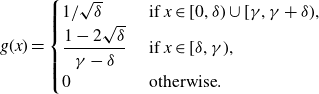 \begin{align*}g(x) = \begin{cases} {}1/\sqrt{\delta} &\text{ if } x \in [0,\delta) \cup [\gamma,\gamma + \delta),\\ {}\dfrac{1 - 2\sqrt{\delta}}{\gamma - \delta} &\text{ if } x \in [\delta,\gamma),\\ {}0 &\text{ otherwise}.\end{cases}\end{align*}
In the case when $\gamma = 1/2$
, we take some
$\gamma = 1/2$
, we take some $0 {\lt} \delta {\lt} 1/2$
and let
$0 {\lt} \delta {\lt} 1/2$
and let
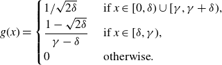 \begin{align*}g(x) = \begin{cases} {}1/\sqrt{2\delta} &\text{ if } x \in [0,\delta) \cup [\gamma,\gamma + \delta),\\ {}\dfrac{1 - \sqrt{2\delta}}{\gamma - \delta} &\text{ if } x \in [\delta,\gamma),\\ {}0 &\text{ otherwise}.\end{cases}\end{align*}
In both cases, it is straightforward to check by elementary computations that the following three statements hold:
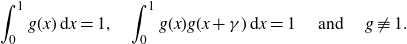 \begin{align*} \int_{0}^1 g(x)\,\mathrm{d}x = 1, \quad \int_{0}^1 g(x)g(x+ \gamma)\,\mathrm{d}x = 1 \quad \text{ and } \quad g \not\equiv 1. \end{align*}
The case when $1/2{\lt}\gamma{\lt}1$
is covered by the first case dealt with earlier, because
$1/2{\lt}\gamma{\lt}1$
is covered by the first case dealt with earlier, because $\gamma$
-PPC is equivalent to
$\gamma$
-PPC is equivalent to $(1-\gamma)$
-PPC. This concludes the proof of Theorem 1·1.
$(1-\gamma)$
-PPC. This concludes the proof of Theorem 1·1.
3. Proof of Theorem 1·3
We first prove the result for $\gamma = 1/2$
and then we explain how the proof can be generalised to values
$\gamma = 1/2$
and then we explain how the proof can be generalised to values $0{\lt}\gamma {\lt} 1/2$
. In both cases, we shall make use of the binary van der Corput sequence
$0{\lt}\gamma {\lt} 1/2$
. In both cases, we shall make use of the binary van der Corput sequence $(c_n)_{n\in \mathbb N}$
that is defined as follows (see also [Reference Kuipers and Niederreiter5]): writing
$(c_n)_{n\in \mathbb N}$
that is defined as follows (see also [Reference Kuipers and Niederreiter5]): writing $n-1 = a_m(n)2^m + \ldots + a_1(n)2 + a_0(n)$
for the binary expansion of the integer
$n-1 = a_m(n)2^m + \ldots + a_1(n)2 + a_0(n)$
for the binary expansion of the integer $n-1$
, the nth term of
$n-1$
, the nth term of $(c_n)_{n\in\mathbb N}$
is the number
$(c_n)_{n\in\mathbb N}$
is the number
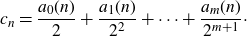 \begin{align*} c_n = \frac{a_0(n)}{2} + \frac{a_1(n)}{2^2} + \cdots + \frac{a_m(n)}{2^{m+1}} \cdot \end{align*}
When $\gamma = 1/2.$
We shall construct a sequence
$\gamma = 1/2.$
We shall construct a sequence $ (x_n)_{n \in \mathbb{N}} \subseteq [0,1]$
that on the one hand is uniformly distributed, which implies
$ (x_n)_{n \in \mathbb{N}} \subseteq [0,1]$
that on the one hand is uniformly distributed, which implies $\int_{0}^1 g(x) g(x-1/2) \,\mathrm{d}x = 1$
, but on the other hand
$\int_{0}^1 g(x) g(x-1/2) \,\mathrm{d}x = 1$
, but on the other hand
 \begin{align*}F_{\frac12}(s) = \liminf_{N\to \infty}\frac{1}{N} \# \Big\{ m,n \leqslant N \;:\; \|x_m - x_n -\frac12 \| \leqslant \frac{s}{N} \Big\} = 0 \qquad \text{for all } s{\gt}0. \end{align*}
We will actually show something stronger: the relation above will hold with limit instead of liminf. We define the auxiliary sequences $(y_n)_{n \in \mathbb{N}}, (z_n)_{n \in \mathbb{N}} $
as follows: we set
$(y_n)_{n \in \mathbb{N}}, (z_n)_{n \in \mathbb{N}} $
as follows: we set $y_n = {1}/{2} c_n$
and
$y_n = {1}/{2} c_n$
and
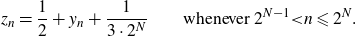 \begin{align*} z_n = \frac{1}{2} + y_n +\frac{1}{3\cdot 2^N} \qquad \text{whenever } 2^{N-1} {\lt} n \leqslant 2^{N}. \end{align*}
By these definitions, it is obvious that $(y_n)_{n \in \mathbb{N}} \subseteq [0,1/2]$
and
$(y_n)_{n \in \mathbb{N}} \subseteq [0,1/2]$
and $(z_n)_{n \in \mathbb{N}} \subseteq [1/2,1]$
.
$(z_n)_{n \in \mathbb{N}} \subseteq [1/2,1]$
.
The sequence $(x_n)_{n \in \mathbb{N}} $
is constructed recursively, with the Nth step involving the definition of the terms
$(x_n)_{n \in \mathbb{N}} $
is constructed recursively, with the Nth step involving the definition of the terms $x_n, \, 2(N-1)2^{N-1} {\lt} n \leqslant 2N2^N.$
At step
$x_n, \, 2(N-1)2^{N-1} {\lt} n \leqslant 2N2^N.$
At step $N = 1$
, we set
$N = 1$
, we set
 \begin{align*}x_1 = y_1, \quad x_2 = z_1,\quad x_3 = y_2, \quad x_4 = z_2.\end{align*}
Assume that for some $N\geqslant 1$
we have defined all points
$N\geqslant 1$
we have defined all points $x_n, 1\leqslant n\leqslant 2N2^{N}.$
Set
$x_n, 1\leqslant n\leqslant 2N2^{N}.$
Set
 \begin{align*} (x_{2N2^N + 1}, \ldots, x_{2(N+1)2^{N}}) = (y_1,z_1,y_2,z_2,\ldots,y_{2^{N}},z_{2^{N}}). \end{align*}
The $2(N+1)2^N$
-tuple
$2(N+1)2^N$
-tuple $(x_{2(N+1)2^N+1},\ldots, x_{2(N+1)2^{N+1}})$
is then defined by concatenating the
$(x_{2(N+1)2^N+1},\ldots, x_{2(N+1)2^{N+1}})$
is then defined by concatenating the $2^{N+1}$
tuple
$2^{N+1}$
tuple
 \begin{align*} (y_{2^{N}+1},z_{2^{N}+1},\ldots,y_{2^{N+1}},z_{2^{N+1}})\end{align*} $N+1$
-times with itself. In that way, for each
$N+1$
-times with itself. In that way, for each $N\geqslant 1$
the terms
$N\geqslant 1$
the terms $x_1,\ldots, x_{2N2^N}$
contain N copies of the points
$x_1,\ldots, x_{2N2^N}$
contain N copies of the points $y_1,\ldots,y_{2^N}$
and N copies of the points
$y_1,\ldots,y_{2^N}$
and N copies of the points $z_1,\ldots, z_{2^N}.$
It is straightforward to check that the sequence $(x_n)_{n \in \mathbb{N}} $
is uniformly distributed, so it remains to prove that
$(x_n)_{n \in \mathbb{N}} $
is uniformly distributed, so it remains to prove that $F_{\frac12}(s)=0$
. For any
$F_{\frac12}(s)=0$
. For any $N\geqslant 1$
, set
$N\geqslant 1$
, set
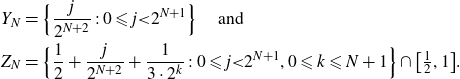 \begin{align*} {}Y_N &= \Big\{\frac{j}{2^{N+2}}\;:\; 0 \leqslant j {\lt} 2^{N+1}\Big\} \quad \text{ and }\\ {}Z_N &= \Big\{\frac{1}{2} + \frac{j}{2^{N+2}} + \frac{1}{3\cdot 2^k}\;:\; 0 \leqslant j {\lt} 2^{N+1}, 0 \leqslant k \leqslant N+1 \Big\} \cap \big[\tfrac12,1\big].\end{align*}
We claim that
 \begin{equation} \Big\lVert a - b - \frac{1}{2}\Big\rVert \geqslant \frac{1/12}{2^N} \qquad \text{ whenever } \quad a,b \in Y_N \cup Z_N. \end{equation}
This is obvious for $a,b \in Y_N$
. Since
$a,b \in Y_N$
. Since
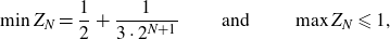 \begin{align*}\min Z_N = \frac{1}{2} + \frac{1}{3\cdot 2^{N+1}}\qquad \text{ and } \qquad \max Z_N \leqslant 1,\end{align*}
the inequality in (3·1) also holds when $a,b \in Z_N$
. It remains to check the case when
$a,b \in Z_N$
. It remains to check the case when $a \in Y_N, b \in Z_N$
(or vice-versa); then
$a \in Y_N, b \in Z_N$
(or vice-versa); then
 \begin{equation*} {}\Big\lVert a - b - \frac{1}{2}\Big\rVert {}\geqslant \min_{0 \leqslant k \leqslant N+1} \min_{n \in \mathbb Z} \Big\lVert \frac{n}{2^{N+2}} - \frac{1}{3\cdot 2^k}\Big\rVert \geqslant \frac{1}{3\cdot 2^{N+2}} = \frac{1/12}{2^{N}},\end{equation*}
since 3 is coprime to $2^N$
. This proves (3·1).
$2^N$
. This proves (3·1).
Now given $M \in \mathbb N$
, let
$M \in \mathbb N$
, let $N = N(M)\geqslant 1$
be defined by
$N = N(M)\geqslant 1$
be defined by
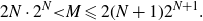 \begin{equation*} {}2N\cdot 2^N {\lt} M \leqslant2 (N+1) 2^{N+1}.\end{equation*}
We then have the inclusion
 \begin{align*}\{x_n\;:\; 1 \leqslant n \leqslant M\} &\subseteq \{y_n\;:\; 1 \leqslant n \leqslant 2^{N+1} \} \cup \{z_n\;:\; 1 \leqslant n \leqslant 2^{N+1} \} \subseteq Y_N \cup Z_N.\end{align*}
Thus for a fixed value of $s {\gt} 0$
, whenever
$s {\gt} 0$
, whenever $ \#\left\{a,b \in Y_N \cup Z_N\;:\; \lVert a- b - 1/2 \rVert \leqslant{s}/{2N\cdot 2^N}\right\}=0,$
then also
$ \#\left\{a,b \in Y_N \cup Z_N\;:\; \lVert a- b - 1/2 \rVert \leqslant{s}/{2N\cdot 2^N}\right\}=0,$
then also $\#\left\{n, m \leqslant M\;:\; \lVert x_n - x_m - 1/2 \rVert \leqslant{s}/{M} \right\}=0$
. Hence for all
$\#\left\{n, m \leqslant M\;:\; \lVert x_n - x_m - 1/2 \rVert \leqslant{s}/{M} \right\}=0$
. Hence for all $N \geqslant 6s$
, (3·1) implies that
$N \geqslant 6s$
, (3·1) implies that $\#\left\{n, m \leqslant M\;:\; \lVert x_n - x_m - 1/2 \rVert \leqslant{s}/{M} \right\}=0$
and we obtain
$\#\left\{n, m \leqslant M\;:\; \lVert x_n - x_m - 1/2 \rVert \leqslant{s}/{M} \right\}=0$
and we obtain $F_{1/2}(s) = 0$
.
$F_{1/2}(s) = 0$
.
When $0 {\lt} \gamma {\lt} 1/2$
. We set
$0 {\lt} \gamma {\lt} 1/2$
. We set $\varepsilon = 2^{-i}$
where
$\varepsilon = 2^{-i}$
where $i\geqslant 1$
is large enough such that
$i\geqslant 1$
is large enough such that $0 {\lt} \varepsilon {\lt} min \{(1/2-\gamma)/2, \gamma\}$
. We then define
$0 {\lt} \varepsilon {\lt} min \{(1/2-\gamma)/2, \gamma\}$
. We then define $(y_n)_{n \in \mathbb{N}} $
and
$(y_n)_{n \in \mathbb{N}} $
and $(z_n)_{n \in \mathbb{N}} $
by setting
$(z_n)_{n \in \mathbb{N}} $
by setting
 \begin{align*} y_n = \varepsilon c_n \qquad \text{and} \qquad z_n = \gamma + y_n + \frac{1}{3\cdot 2^N}\quad \text{whenever } 2^{N-1} {\lt} n \leqslant 2^N.\end{align*}
The sequence $(x_n)_{n \in \mathbb{N}} $
is then defined precisely as in the case
$(x_n)_{n \in \mathbb{N}} $
is then defined precisely as in the case $\gamma = 1/2$
.
$\gamma = 1/2$
.
One can use the same arguments as before to show that for any $s{\gt}0$
we have
$s{\gt}0$
we have $F_\gamma(s)=0.$
On the other hand, the asymptotic density function of
$F_\gamma(s)=0.$
On the other hand, the asymptotic density function of $(x_n)_{n \in \mathbb{N}} $
is
$(x_n)_{n \in \mathbb{N}} $
is
 \begin{align*}g(x) = \begin{cases} 1/(2\varepsilon), & \text{ if } x\in [0,\varepsilon]\cup [\gamma,\gamma + \varepsilon] \\ 0, & \text{ otherwise} \end{cases} \end{align*}
and thus $ \int_{0}^1 g(x)g(x+\gamma) \mathrm{d}x = 1/(4\varepsilon) {\gt} 0, $
which concludes the proof.
$ \int_{0}^1 g(x)g(x+\gamma) \mathrm{d}x = 1/(4\varepsilon) {\gt} 0, $
which concludes the proof.
Remark 3·1. Note that the sequence defined above for $\gamma \neq 1/2$
is not uniformly distributed. However, one could adapt the construction by “diluting” the sequence with i.i.d. samples on
$\gamma \neq 1/2$
is not uniformly distributed. However, one could adapt the construction by “diluting” the sequence with i.i.d. samples on $[\varepsilon,\gamma] \cup [\gamma + \varepsilon,1]$
in order to get a sequence that almost surely is uniformly distributed mod 1 and satisfies
$[\varepsilon,\gamma] \cup [\gamma + \varepsilon,1]$
in order to get a sequence that almost surely is uniformly distributed mod 1 and satisfies
 \begin{align*}\limsup_{s\to \infty} \frac{F_\gamma(s)}{2s} {\lt} \int_0^1 g(x)g(x+\gamma)\,\mathrm{d}x = 1.\end{align*}
We leave the details to the interested reader.
4.
$\gamma_1$
- PPC does not imply
$\gamma_2$
- PPC


We finish with the proof of Theorem 1·4. Let $(x_n)_{n \in \mathbb{N}} $
be a sequence of independent random variables, following the uniform distribution in [0, 1]. Define
$(x_n)_{n \in \mathbb{N}} $
be a sequence of independent random variables, following the uniform distribution in [0, 1]. Define $(y_n)_{n \in \mathbb{N}} $
by
$(y_n)_{n \in \mathbb{N}} $
by
 \begin{align*} y_{2n-1} = x_n \quad \text{and} \quad y_{2n} = x_n +\gamma_2 \qquad (n\geqslant 1).\end{align*}
In what follows, we will write $R_2^{\mathcal{X}}$
and
$R_2^{\mathcal{X}}$
and $R_2^{\mathcal{Y}}$
for the pair correlation functions of
$R_2^{\mathcal{Y}}$
for the pair correlation functions of $(x_n)_{n \in \mathbb{N}} $
and
$(x_n)_{n \in \mathbb{N}} $
and $(y_n)_{n \in \mathbb{N}} $
respectively. Then by definition of
$(y_n)_{n \in \mathbb{N}} $
respectively. Then by definition of $(y_n)_{n \in \mathbb{N}} $
,
$(y_n)_{n \in \mathbb{N}} $
,
 \begin{align*} R_2^{\mathcal{Y}}(\gamma_2;\;s,2N) = \frac{1}{2N}\#\Big\{n \neq m \leqslant 2N\;:\; \lVert y_n - y_m - \gamma_2 \rVert \leqslant \frac{s}{2N}\Big\}\geqslant \frac{1}{2N} N = \frac{1}{2} \cdot\end{align*}
Taking $s {\lt} {1}/{4}$
, the above shows that
$s {\lt} {1}/{4}$
, the above shows that $(y_n)_{n \in \mathbb{N}} $
does not have
$(y_n)_{n \in \mathbb{N}} $
does not have $\gamma_2$
- PPC. We claim that
$\gamma_2$
- PPC. We claim that $(y_n)_{n \in \mathbb{N}} $
has still almost surely
$(y_n)_{n \in \mathbb{N}} $
has still almost surely $\gamma_1$
- PPC: we have
$\gamma_1$
- PPC: we have
 \begin{equation*} {}\begin{split}R_2^{\mathcal{Y}}(\gamma_1;\;s,2N) &= \frac{1}{2N}\#\Big\{n\neq m \leqslant 2N\;:\; \lVert y_n - y_m -\gamma_1 \rVert \leqslant \frac{s}{2N}\Big\} {} {}\\& = \frac{1}{2N}\#\Big\{n \neq m \leqslant N\;:\; \lVert x_n - x_m -\gamma_1 \rVert \leqslant \frac{s/2}{N}\Big\} {} {}\\&\qquad +\frac{1}{2N}\#\Big\{n\neq m \leqslant N\;:\; \lVert x_n + \gamma_2 - (x_m + \gamma_2) - \gamma_1 \rVert \leqslant \frac{s/2}{N}\Big\} {} {}\\& \qquad + \frac{1}{2N}\#\Big\{n,m \leqslant N\;:\; \lVert x_n + \gamma_2 - x_m -\gamma_1 \rVert \leqslant \frac{s/2}{N}\Big\} {} {}\\& \qquad + \frac{1}{2N}\#\Big\{n,m \leqslant N\;:\; \lVert x_n - (x_m + \gamma_2) -\gamma_1 \rVert \leqslant \frac{s/2}{N}\Big\} {} {}\\&= R_2^{\mathcal{X}}(\gamma_1;\frac{s}{2},N) + \frac12 R_2^{\mathcal{X}}(\gamma_1-\gamma_2; \frac{s}{2}, N) + \frac12 R_2^{\mathcal{X}}(\gamma_1+\gamma_2; \frac{s}{2}, N) {} {}\\&\qquad + \frac{1}{2N}\#\Big\{n \leqslant N\;:\; \lVert x_n + \gamma_2 - x_n -\gamma_1 \rVert \leqslant \frac{s/2}{N}\Big\} {} {}\\& \qquad + \frac{1}{2N}\#\Big\{n \leqslant N\;:\; \lVert x_n - (x_n + \gamma_2) -\gamma_1 \rVert \leqslant \frac{s/2}{N}\Big\}. {}\end{split}\end{equation*}
Since $\gamma_1 - \gamma_2, \gamma_1 + \gamma_2 \notin \mathbb{Z}$
, the last two terms in the above equation vanish if N is sufficiently large. By Theorem 1·2, the sequence
$\gamma_1 - \gamma_2, \gamma_1 + \gamma_2 \notin \mathbb{Z}$
, the last two terms in the above equation vanish if N is sufficiently large. By Theorem 1·2, the sequence $(x_n)_{n \in \mathbb{N}} $
has
$(x_n)_{n \in \mathbb{N}} $
has $\gamma_1$
- PPC and
$\gamma_1$
- PPC and $(\gamma_1-\gamma_2)$
- PPC and
$(\gamma_1-\gamma_2)$
- PPC and $(\gamma_1+\gamma_2)$
- PPC almost surely, therefore with probability 1 we have
$(\gamma_1+\gamma_2)$
- PPC almost surely, therefore with probability 1 we have
 \begin{align*}\lim_{N \to \infty} R_2^\mathcal{Y}(\gamma_1;\;s,2N) = 2s \qquad \text{ for all } s{\gt}0. \end{align*}
A standard approximation argument now gives that $\lim_{N\to \infty}R_2^\mathcal{Y}(\gamma_1;\;s,N) =2s$
for all scales
$\lim_{N\to \infty}R_2^\mathcal{Y}(\gamma_1;\;s,N) =2s$
for all scales $s{\gt}0$
, which means that
$s{\gt}0$
, which means that $(y_n)_{n \in \mathbb{N}} $
has
$(y_n)_{n \in \mathbb{N}} $
has $\gamma_1$
- PPC almost surely.
$\gamma_1$
- PPC almost surely.
Acknowledgements
MH is supported by the EPSRC grant EP/X030784/1. A part of this work was supported by the Swedish Research Council under grant no. 2016-06596 while MH was in residence at Institut Mittag-Leffler in Djursholm, Sweden in 2024. AZ is supported by European Research Council (ERC) under the European Union’s Horizon 2020 Research and Innovation Program, Grant agreement no. 754475.

 Open access