1. Introduction
The reliability of system refers to the probability that system will effectively carry out its intended function within a designated time frame and under specified environmental conditions. In the reliability context, the germ of stress–strength model was initially introduced by [Reference Birnbaum8] and developed by [Reference Birnbaum and McCarty9] and [Reference Church and Harris11]. This model involves assessing the reliability of a system with a random strength variable X and suffering from random stress variable Y. The reliability of the system, considering the stress–strength relationship as the failure mode, is defined as the probability that the strength variable X exceeds the stress variable Y. The stress–strength model has found applications in a wide array of fields, including engineering, oceanography, hydrology, economics, and medicine, as described by [Reference Kotz, Pensky and Lumelskii21]. The following examples highlight the practical applications of the stress–strength model in diverse fields, demonstrating its significance in assessing systems reliability.
Rocket engines: Here X is assigned to denote the strength of the rocket chamber while Y commonly signifies the maximal chamber pressure generated by ignition of a solid propellant. In this scenario, the reliability R can be defined as the probability of a successful engine firing, defined as ![]() $P(X \gt Y)$.
$P(X \gt Y)$.
Earthquake resistance: In a study of the risk of some tall or spacious buildings, it is crucial to evaluate the building’s capacity to withstand the stresses induced by ground motion during an earthquake. When considering the random variable X as the building strength during an earthquake and the random variable Y as the induced stress, the probability ![]() $R=P(X \gt Y)$ quantifies the probability of designing a building that is deemed safe.
$R=P(X \gt Y)$ quantifies the probability of designing a building that is deemed safe.
Several studies in the literature have explored stress–strength models using various probability distributions, including Weibull, Lindley, generalized logistic, and bathtub-shaped distributions. Noteworthy recent contributions on this topic include works by [Reference Asgharzadeh, Valiollahi and Raqab3, Reference Babayi, Khorram and Tondro4, Reference Khan and Jan18], and [Reference Shoaee and Khorram30].
The previously mentioned system is considered to be a single-component system, which is a limited assumption when addressing various scenarios. As science, technology, and manufacturing techniques have advanced, we now encounter numerous multicomponent systems in our daily lives, including items like IT hardware, aero engines, keyboards, and more. The study of multicomponent system reliability in stress–strength models holds significant value and provides meaningful insights. Eryilmaz [Reference Eryilmaz14] obtained the system reliability for a general coherent structure under stress–strength setup. Eryilmaz and Iscioglu [Reference Eryilmaz and Iscioglu15] got some conclusions about stress–strength reliability in the context of multicomponent multi-state systems modeling. Reliability inference of k-out-of-n system for multicomponent stress–strength model under the assumptions of Burr-XII distribution was studied by [Reference Rao, Aslam and Kundu28]. Liu et al. [Reference Liu, Shi, Bai and Zhan22] derived the reliability estimation of multicomponent system accounting for the stress–strength model and the specific N-M-cold-standby arrangement. Kohansal [Reference Kohansal20] focused on the estimation of system reliability for a k-out-of-n system within a multicomponent stress–strength model, employing progressively censored Kumaraswamy sample. The parallel-series system, an essential and widely used structure in reliability engineering, consists of several subsystems connected in parallel, each containing numerous components arranged in a series configuration, as illustrated in Figure 1. The parallel-series system is vital for ensuring high reliability, robust fault tolerance, and versatile operation, making it indispensable for critical applications like power grids, communication infrastructures, and aerospace technologies. For further studies on parallel-series systems, readers may refer to [Reference Nadarajah, Abdel-Hamid and Hashem26] and [Reference Abdel-Hamid and Hashem2]. In the domain of reliability estimation for parallel-series systems, several researchers have proposed flexible methodologies. For instance, Coit [Reference Coit12] described a flexible procedure to establish approximate confidence interval (ACI) for system reliability in situations there is uncertainty about component reliability information. Benkamra et al. [Reference Benkamra, Terbeche and Tlemcani7] constructed a properly hybrid sequential design to optimize the reliability of the parallel-series system. Modibbo et al. [Reference Modibbo, Arshad, Abdalghani and Ali23] introduced two approaches of estimations for the parallel-series and series-parallel system reliability developed on the maximum likelihood estimation (MLE) and uniformly minimum-variance unbiased estimation.
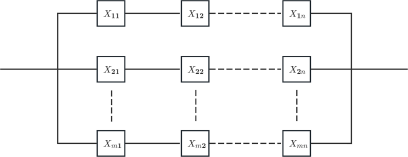
Figure 1. The structure of a parallel-series system.
Traditionally, it has been commonly assumed that the stress and strength variables in reliability analysis are independent of each other. However, in practical scenarios, considering the dependence structure between stress and strength variables is often more realistic due to their potential influence from shared or common factors. An effective approach for modeling the dependence structure between these variables is through the use of a bivariate distribution, such as bivariate Gamma distribution [Reference Nadarajah25], Marshall–Olkin bivariate Weibull distribution [Reference Nadar and Kizilaslan24], general bivariate distribution [Reference Abdel-Hamid1], bivariate Kumaraswamy distribution [Reference Kizilaslan and Nadar19], and bivariate exponentiated half-logistic distribution [Reference Xavier and Jose31]. However, one limitation of the bivariate distribution model is that it necessitates the marginal distributions of the stress and strength variables to be from the same family of distributions. To overcome this constraint, copula has been widely utilized as a potent tool for capturing the dependence structure between stress and strength variables. Copula is utilized to characterize the dependence structure among random variables and holds a significant position in the formation of joint distributions by leveraging marginal distributions. The absence of marginal distribution information within copula empowers the ability to exercise greater freedom in choosing the marginal distribution. In Domma and Giordano’s works [Reference Domma and Giordano13], the dependence relationship was characterized by Farlie-Gumbel-Morgenstern (FGM) copula. By considering Burr III distributions for both stress and strengths, they obtained the reliability estimator. Gao et al. [Reference Gao, An and Liu16] conducted a comprehensive evaluation of reliability while considering the mixed copula dependence structure between stress and strength variables by combining the Frank, Clayton, and Gumbel copulas through a linear combination. Estimation of the stress–strength reliability was investigated by [Reference Bai, Shi, Liu and Liu6] when stress and strength were Gumbel copula dependent. Zhu [Reference Zhu32] derived the reliability estimation of k-out-of-n system for a dependent multicomponent stress–strength model under the assumption of Clayton copula dependence between stress and strength variables.
Although prior studies have addressed reliability estimation for parallel-series systems, to the best of our knowledge, there are few works available on dependent stress–strength models specifically applied to parallel-series systems. Therefore, this paper aims to provide reliability estimation for the dependent stress–strength model in a parallel-series system, considering the dependence between the stress and strength variables, assuming Weibull and Burr XII distributions for stress and strength, respectively. We employ copula function to capture the dependence between the two variables. The two-step MLE and maximum product spacing (MPS) approaches are used to estimate unknown parameters and system reliability. That is, in the first step of the two-step approach, the focus is on estimating the model parameters. Following this, the second step involves estimating the dependence parameter utilizing the results obtained in the initial step. The system reliability is subsequently determined using the estimated model parameters and dependence parameter. Confidence intervals (CIs) for both unknown parameters and system reliability are established by taking advantage of the asymptotic normality of MLEs and utilizing the bootstrap percentile methods.
The rest of this paper is rolled as follows. In Section 2, we introduce the copula theory and derive the reliability of parallel-series system. In Section 3, the two-step MLE and MPS approaches are employed to calculate the reliability estimators for the parallel-series system. In Section 4, the CIs for both unknown parameters and system reliability are also developed utilizing bootstrap method. A Monte Carlo simulation study is carried out in Section 5 to compare the effectiveness of the proposed inference methods. In Section 6, we analyze a real dataset for illustrative purposes. Section 7 concludes the paper.
2. Preliminaries
Prior to delving into the main results, it is crucial to provide an overview of basic concepts that will be referenced throughout the subsequent sections.
2.1. Copula
For a random vector ![]() $\boldsymbol{X}=(X_1,X_2,\ldots,X_n)$ with joint cumulative distribution function
$\boldsymbol{X}=(X_1,X_2,\ldots,X_n)$ with joint cumulative distribution function ![]() $(\operatorname{CDF}) \ H$ and univariate marginal distribution functions
$(\operatorname{CDF}) \ H$ and univariate marginal distribution functions ![]() $F_1,F_2,\ldots,F_n$, if there exists a function
$F_1,F_2,\ldots,F_n$, if there exists a function ![]() $C:[0,1]^n\to [0,1]$, such that, for all
$C:[0,1]^n\to [0,1]$, such that, for all ![]() $x_{i}, i=1,\dots,n$,
$x_{i}, i=1,\dots,n$,
then C is called the copula of random vector X. Similarly, if there exists a function ![]() $\hat{C}:[0,1]^n\to [0,1]$, such that
$\hat{C}:[0,1]^n\to [0,1]$, such that
where ![]() ${\overline F}_i=1-F_i$ is marginal survival function and
${\overline F}_i=1-F_i$ is marginal survival function and ![]() ${\overline H}$ is the joint survival function, then
${\overline H}$ is the joint survival function, then ![]() $\widehat{C}$ is called the survival copula of random vector X.
$\widehat{C}$ is called the survival copula of random vector X.
Copulas have many good properties, some main properties are given below, note ![]() $u_{i}=F_{i}(x_{i}),\ i=1,\dots,n$,
$u_{i}=F_{i}(x_{i}),\ i=1,\dots,n$,
(i) If at least one ![]() $u_{i}, i=1,\dots,n$ is equal to zero, then
$u_{i}, i=1,\dots,n$ is equal to zero, then
(ii) If all ![]() $u_{i}, i=1,\dots,n$ are equal to 1 except ui, then
$u_{i}, i=1,\dots,n$ are equal to 1 except ui, then
Archimedean copulas are favored in various applications owing to their mathematical tractability and capacity to model wide ranges of dependence structures. The Archimedean copula family encompasses numerous useful copulas, including well-known examples such as product copula, Clayton copula, Frank copula, and Gumbel copula. The detailed description of Archimedean copula is given as follows:
For a decreasing and continuous function ![]() $\psi:[0,+\infty )\mapsto [0,1]$ such that
$\psi:[0,+\infty )\mapsto [0,1]$ such that ![]() $\psi(0)=1$ and
$\psi(0)=1$ and ![]() $\psi(+\infty )=0.$ Then
$\psi(+\infty )=0.$ Then
is said to be an Archimedean copula with generator ψ, where ![]() $\phi =\psi^{-1}$ is the pseudo-inverse of ψ. A comprehensive exploration of copulas and their applications can be found in [Reference Nelsen27].
$\phi =\psi^{-1}$ is the pseudo-inverse of ψ. A comprehensive exploration of copulas and their applications can be found in [Reference Nelsen27].
The two-dimensional strict Clayton copula
 \begin{align}
C_{\theta}(u, v)=\left(u^{-\theta}+v^{-\theta}-1\right)^{-\frac{1}{\theta}}, ~~\theta \in(0,+\infty),
\end{align}
\begin{align}
C_{\theta}(u, v)=\left(u^{-\theta}+v^{-\theta}-1\right)^{-\frac{1}{\theta}}, ~~\theta \in(0,+\infty),
\end{align}which is used in this paper to capture the dependence structure between the stress and strength. The dependence between two random variables decreases as θ decreases, and the first partial derivative of (1) with respect to u can be written as
 \begin{equation*}
\frac{\partial C_{\theta}(u, v)}{\partial u}=u^{-(\theta+1)}\left(u^{-\theta}+v^{-\theta}-1\right)^{-\left(\frac{1}{\theta}+1\right)}.
\end{equation*}
\begin{equation*}
\frac{\partial C_{\theta}(u, v)}{\partial u}=u^{-(\theta+1)}\left(u^{-\theta}+v^{-\theta}-1\right)^{-\left(\frac{1}{\theta}+1\right)}.
\end{equation*}2.2. Model description
Consider an m-n parallel-series system consisting of m disjoint modules connected in parallel. Module i ![]() $ (1\leq i\leq m)$ consisting of n components connected in series. Let
$ (1\leq i\leq m)$ consisting of n components connected in series. Let ![]() $X_{ij} (i=1,2,\dots,m; j=1,2, \ldots, n)$ denote a set of independent and identically distributed random variables with common CDF F, representing the strength of component in the m-n parallel-series system. Additionally, let Y be a random variable representing the common stress, and it has a CDF G. For an m-n parallel-series system, denoting the strength of system by Z, then the
$X_{ij} (i=1,2,\dots,m; j=1,2, \ldots, n)$ denote a set of independent and identically distributed random variables with common CDF F, representing the strength of component in the m-n parallel-series system. Additionally, let Y be a random variable representing the common stress, and it has a CDF G. For an m-n parallel-series system, denoting the strength of system by Z, then the ![]() $\operatorname{CDF} $ of Z is given by
$\operatorname{CDF} $ of Z is given by
and its probability density function ![]() $(\operatorname{PDF})$ can be written as
$(\operatorname{PDF})$ can be written as
Suppose that ![]() $X_{ij} (i=1,2,\dots,m; j=1,2, \ldots, n)$ follows Burr XII distribution with shape parameters λ and δ, Y follows Weibull distribution with scale parameter α and shape parameter β. The corresponding distribution functions are
$X_{ij} (i=1,2,\dots,m; j=1,2, \ldots, n)$ follows Burr XII distribution with shape parameters λ and δ, Y follows Weibull distribution with scale parameter α and shape parameter β. The corresponding distribution functions are
 \begin{align*}
&F\left(x ;\lambda, \delta \right)=1-\left(1+x^{\lambda}\right)^{-\delta} , x \gt 0, \lambda \gt 0, \delta \gt 0
\end{align*}
\begin{align*}
&F\left(x ;\lambda, \delta \right)=1-\left(1+x^{\lambda}\right)^{-\delta} , x \gt 0, \lambda \gt 0, \delta \gt 0
\end{align*}and
 \begin{align*}
&G\left(y ; \alpha, \beta \right)=1-\exp \left(-\alpha y^{\beta}\right), y \gt 0, \alpha \gt 0, \beta \gt 0.
\end{align*}
 Then, the respective ![]() $\operatorname{PDF}$ are
$\operatorname{PDF}$ are
 \begin{align*}
&f(x ; \lambda, \delta)=\delta\lambda x^{\lambda-1} \left(1+x^{\lambda}\right)^{-\delta-1}
\end{align*}
\begin{align*}
&f(x ; \lambda, \delta)=\delta\lambda x^{\lambda-1} \left(1+x^{\lambda}\right)^{-\delta-1}
\end{align*}and
 \begin{align*}
g\left(y ; \alpha, \beta\right)=\alpha \beta y^{\beta-1} \exp \left(-\alpha y^{\beta}\right).
\end{align*}
\begin{align*}
g\left(y ; \alpha, \beta\right)=\alpha \beta y^{\beta-1} \exp \left(-\alpha y^{\beta}\right).
\end{align*}Hence, (2) and (3) can be expressed as
and
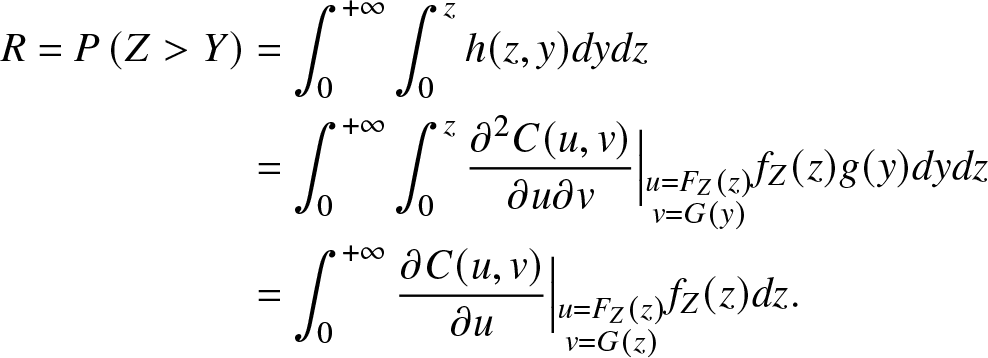
In the majority of cases, stress variable Y and strength variable Z exhibit dependence. To account for this dependence, we assume that their relationship is characterized by a two-dimensional Clayton copula ![]() $C_{\theta}(u, v)$. Then, the reliability R of the system is expressed as
$C_{\theta}(u, v)$. Then, the reliability R of the system is expressed as
 \begin{align}
R=P\left(Z \gt Y\right)&=\int_{0}^{+\infty} \int_{0}^{z} h(z, y) dy dz \nonumber\\
& =\int_{0}^{+\infty} \int_{0}^{z} \frac{\partial^{2} C(u, v)}{\partial u \partial v} \Big | _{\substack{u=F_{Z}(z) \\ v=G(y)}}{}f_{Z}(z) g(y)dy dz \nonumber\\
& =\int_{0}^{+\infty} \frac{\partial C(u, v)}{\partial u} \Big | _{\substack{u=F_{Z}(z) \\ v=G(z)}}{} f_{Z}(z) dz.
\end{align}
\begin{align}
R=P\left(Z \gt Y\right)&=\int_{0}^{+\infty} \int_{0}^{z} h(z, y) dy dz \nonumber\\
& =\int_{0}^{+\infty} \int_{0}^{z} \frac{\partial^{2} C(u, v)}{\partial u \partial v} \Big | _{\substack{u=F_{Z}(z) \\ v=G(y)}}{}f_{Z}(z) g(y)dy dz \nonumber\\
& =\int_{0}^{+\infty} \frac{\partial C(u, v)}{\partial u} \Big | _{\substack{u=F_{Z}(z) \\ v=G(z)}}{} f_{Z}(z) dz.
\end{align}3. Inference of R
3.1. Maximum likelihood estimation
In this subsection, our focus is on the MLE of R. Suppose that there are k systems subjected to a life-testing process, and the observed samples of the system stress and strength are Yi and Zi ![]() $(i=1,2, \ldots, k)$, respectively. Hence the respective likelihood functions with observed samples Zi and Yi
$(i=1,2, \ldots, k)$, respectively. Hence the respective likelihood functions with observed samples Zi and Yi ![]() $ (i=1,2, \ldots, k)$ are
$ (i=1,2, \ldots, k)$ are
 \begin{align*}
L_{1}(\lambda, \delta\mid\text{data})&=\prod_{i=1}^{k} f_{Z}\left(z_{i} ; \lambda,\delta\right)
=n^k m^k{\delta}^k{\lambda}^k \prod_{i=1}^{k}z_{i}^{\lambda-1}(1+z_{i}^{\lambda})^{-n\delta-1}[1-(1+z_{i}^{\lambda})^{-n\delta}]^{m-1}
\end{align*}
\begin{align*}
L_{1}(\lambda, \delta\mid\text{data})&=\prod_{i=1}^{k} f_{Z}\left(z_{i} ; \lambda,\delta\right)
=n^k m^k{\delta}^k{\lambda}^k \prod_{i=1}^{k}z_{i}^{\lambda-1}(1+z_{i}^{\lambda})^{-n\delta-1}[1-(1+z_{i}^{\lambda})^{-n\delta}]^{m-1}
\end{align*}and
 \begin{align*}
L_{2}(\alpha, \beta \mid\text {data})=\prod_{i=1}^{k} g\left(y_{i} ; \alpha, \beta\right)
={\alpha}^k{\beta}^k\prod_{i=1}^{k}y_{i}^{\beta-1}\exp (-\alpha y_{i}^{\beta}).
\end{align*}
\begin{align*}
L_{2}(\alpha, \beta \mid\text {data})=\prod_{i=1}^{k} g\left(y_{i} ; \alpha, \beta\right)
={\alpha}^k{\beta}^k\prod_{i=1}^{k}y_{i}^{\beta-1}\exp (-\alpha y_{i}^{\beta}).
\end{align*}Then, we can further get the respective log-likelihood functions
 \begin{align}
\log L_{1}(\lambda, \delta\mid \text {data})=\; & k \log n+ k\log m + k \log \delta + k\log \lambda -(n\delta+1)\sum_{i=1}^{k}\log(1+z_{i}^{\lambda})
\nonumber \\
& + (\lambda -1)\sum_{i=1}^{k} \log z_{i} + (m-1)\sum_{i=1}^{k}\log [1-(1+z_{i}^{\lambda})^{-n\delta}]
\end{align}
\begin{align}
\log L_{1}(\lambda, \delta\mid \text {data})=\; & k \log n+ k\log m + k \log \delta + k\log \lambda -(n\delta+1)\sum_{i=1}^{k}\log(1+z_{i}^{\lambda})
\nonumber \\
& + (\lambda -1)\sum_{i=1}^{k} \log z_{i} + (m-1)\sum_{i=1}^{k}\log [1-(1+z_{i}^{\lambda})^{-n\delta}]
\end{align}and
 \begin{align}
\log L_{2}(\alpha, \beta \mid \text {data})= k \log \alpha+k \log \beta+(\beta-1) \sum_{i=1}^{k} \log y_{i}-\alpha \sum_{i=1}^{k} y_{i}^{\beta}.
\end{align}
\begin{align}
\log L_{2}(\alpha, \beta \mid \text {data})= k \log \alpha+k \log \beta+(\beta-1) \sum_{i=1}^{k} \log y_{i}-\alpha \sum_{i=1}^{k} y_{i}^{\beta}.
\end{align}The following Theorems 3.1–3.4 affirm the existence and uniqueness of the MLEs of model parameters.
Theorem 3.1. The MLE of λ exists and is unique which is the solution of
 \begin{eqnarray}
J_{1}(\lambda)&=&\frac{k}{\lambda }+ \sum _{i=1}^k \log \left(z_i\right)-(n\delta +1) \sum _{i=1}^k \frac{z_i^{\lambda } \log \left(z_i\right)}{1+z_i^{\lambda }} \nonumber\\
&&+(m-1) \sum _{i=1}^k \frac{n \delta\log \left(z_i\right) z_i^{\lambda }\left(1+z_i^{\lambda }\right){}^{-1-n \delta }}{1-\left(1+z_i^{\lambda }\right){}^{-n \delta }}=0.
\end{eqnarray}
\begin{eqnarray}
J_{1}(\lambda)&=&\frac{k}{\lambda }+ \sum _{i=1}^k \log \left(z_i\right)-(n\delta +1) \sum _{i=1}^k \frac{z_i^{\lambda } \log \left(z_i\right)}{1+z_i^{\lambda }} \nonumber\\
&&+(m-1) \sum _{i=1}^k \frac{n \delta\log \left(z_i\right) z_i^{\lambda }\left(1+z_i^{\lambda }\right){}^{-1-n \delta }}{1-\left(1+z_i^{\lambda }\right){}^{-n \delta }}=0.
\end{eqnarray}Proof. By computing the first partial derivative of (5) with respect to λ, and set to be zero, (7) is obtained. It is easy to figure out that ![]() $\lim _{\lambda \rightarrow 0^{+}}J_{1}(\lambda)=+\infty$. Note that,
$\lim _{\lambda \rightarrow 0^{+}}J_{1}(\lambda)=+\infty$. Note that,  $\lim _{\lambda \rightarrow+\infty} \frac{k}{\lambda }=0$. For convenience, let
 \begin{equation*} J_{11}(\lambda)= \sum _{i=1}^k \log \left(z_i\right)-(n\delta +1) \sum _{i=1}^k \frac{z_i^{\lambda } \log \left(z_i\right)}{1+z_i^{\lambda }} +(m-1) \sum _{i=1}^k \frac{n \delta\log \left(z_i\right) z_i^{\lambda }\left(1+z_i^{\lambda }\right){}^{-1-n \delta }}{1-\left(1+z_i^{\lambda }\right){}^{-n \delta }}.\end{equation*}
 In the next, we just need to show that ![]() $\lim _{\lambda \rightarrow+\infty} J_{11}(\lambda) \lt 0$, the proof will be proceeded by discussing the following three cases.
$\lim _{\lambda \rightarrow+\infty} J_{11}(\lambda) \lt 0$, the proof will be proceeded by discussing the following three cases.
Case 1: ![]() $0 \lt z_{i} \lt 1, i=1,\dots, k.$
$0 \lt z_{i} \lt 1, i=1,\dots, k.$
Observe that ![]() $\log \left(z_i\right) \lt 0$ and
$\log \left(z_i\right) \lt 0$ and ![]() $\lim _{\lambda \rightarrow+\infty} z_{i}^{\lambda}=0,$ thus we have
$\lim _{\lambda \rightarrow+\infty} z_{i}^{\lambda}=0,$ thus we have
 \begin{equation*}\lim _{\lambda \rightarrow+\infty} J_{11}(\lambda) = (1+ \frac{1}{n \delta})\sum _{i=1}^k \log \left(z_i\right) \lt 0.\end{equation*}
 Case 2: ![]() $z_{i} \gt 1, i=1,\dots, k.$
$z_{i} \gt 1, i=1,\dots, k.$
Since ![]() $\log \left(z_i\right) \gt 0$ and
$\log \left(z_i\right) \gt 0$ and  $\lim _{\lambda \rightarrow+\infty} z_{i}^{\lambda}=+\infty$, then we have
 \begin{equation*}\lim _{\lambda \rightarrow+\infty} J_{11}(\lambda) = -n \delta \sum _{i=1}^k \log \left(z_i\right) \lt 0.\end{equation*}
 Case 3: ![]() $0 \lt z_{i} \lt 1 (i=1,\dots, k_{1}),$
$0 \lt z_{i} \lt 1 (i=1,\dots, k_{1}),$ ![]() $z_{j} \gt 1 (j=k_{1}+1,\dots, k).$
$z_{j} \gt 1 (j=k_{1}+1,\dots, k).$
For this case, according to Case 1 and Case 2, we have
 \begin{equation*}\lim _{\lambda \rightarrow+\infty} J_{11}(\lambda) = (1+ \frac{1}{n \delta})\sum _{i=1}^{k_{1}} \log \left(z_i\right) -n\delta \sum _{j=k_{1}+1}^k \log \left(z_j\right) \lt 0.\end{equation*}
 Hence we further get ![]() $\lim _{\lambda \rightarrow+\infty} J_{1}(\lambda) \lt 0$. By noting that
$\lim _{\lambda \rightarrow+\infty} J_{1}(\lambda) \lt 0$. By noting that
 \begin{equation*}n \delta z_i^{\lambda } \left(1+z_i^{\lambda }\right){}^{n \delta }-\left(1+z_i^{\lambda }\right){}^{n\delta }+1\ge0,\end{equation*}
then we get
 \begin{eqnarray*}
\frac{\mathrm d J_{1}(\lambda )}{\mathrm d\lambda}&=&-\frac{k}{\lambda ^2}-(m-1)\sum _{i=1}^n\frac{n \delta z_i^{\lambda } \log ^2\left(z_i\right) \left(n \delta z_i^{\lambda } \left(1+z_i^{\lambda }\right){}^{n \delta }-\left(1+z_i^{\lambda }\right){}^{n\delta }+1\right)}{\left(1+z_i^{\lambda }\right){}^2 \left(\left(1+z_i^{\lambda }\right){}^{n \delta}-1\right){}^2}\nonumber\\
&&-(n \delta +1) \sum _{i=1}^n \frac{z_i^{\lambda } \log ^2\left(z_i\right)}{\left(1+z_i^{\lambda }\right){}^2} \lt 0,
\end{eqnarray*}
 which yields that ![]() $J_{1}(\lambda)$ is decreasing in λ. Thus, the existence and uniqueness of MLE of λ are proved.
$J_{1}(\lambda)$ is decreasing in λ. Thus, the existence and uniqueness of MLE of λ are proved.
Theorem 3.2. The MLE of δ exists and is unique which is the solution of
 \begin{align}
J_{2}(\delta)=\frac{k}{\delta }-n \sum _{i=1}^k \log \left(1+z_i^{\lambda }\right)+(m-1) \sum _{i=1}^k \frac{n \left(1+z_i^{\lambda }\right){}^{-n \delta }\log \left(1+z_i^{\lambda }\right) }{1-\left(1+z_i^{\lambda }\right){}^{-n \delta }}=0.
\end{align}
\begin{align}
J_{2}(\delta)=\frac{k}{\delta }-n \sum _{i=1}^k \log \left(1+z_i^{\lambda }\right)+(m-1) \sum _{i=1}^k \frac{n \left(1+z_i^{\lambda }\right){}^{-n \delta }\log \left(1+z_i^{\lambda }\right) }{1-\left(1+z_i^{\lambda }\right){}^{-n \delta }}=0.
\end{align}Proof. By taking the first partial derivative of (5) with respect to δ, and set to be zero, we have (8). It is easy to verify that ![]() $\lim _{\delta \rightarrow 0^{+}}J_{2}(\delta )=+\infty$ and
$\lim _{\delta \rightarrow 0^{+}}J_{2}(\delta )=+\infty$ and  $\lim _{\delta \rightarrow+\infty} J_{2}(\delta ) = -n \sum _{i=1}^k \log \left(1+z_i^{\lambda }\right) \lt 0.$ Note that
 \begin{eqnarray*}
\frac{\mathrm d J_{2}(\delta )}{\mathrm d\delta }&=&-\frac{k}{\delta ^2}-(m-1) \sum _{i=1}^k \left(-\frac{n^2 \left(1+z_i^{\lambda }\right){}^{-n \delta }\log ^2\left(1+z_i^{\lambda }\right) }{1-\left(1+z_i^{\lambda }\right){}^{-n\delta }}-\frac{n^2 \left(1+z_i^{\lambda }\right){}^{-2n \delta }\log ^2\left(1+z_i^{\lambda }\right)}{\left(1-\left(1+z_i^{\lambda }\right){}^{-n\delta }\right){}^2}\right)\\
&=&-\frac{k}{\delta ^2}-(m-1) \sum _{i=1}^k \left(\frac{n^2 \left(1+z_i^{\lambda }\right){}^{n \delta }\log ^2\left(1+z_i^{\lambda }\right) }{\left(\left(1+z_i^{\lambda }\right){}^{\delta n}-1\right){}^2}\right) \lt 0,
\end{eqnarray*}
 That is, the function ![]() $J_{2}(\delta)$ is decreasing in δ. Hence, the existence and uniqueness of MLE of δ are proved.
$J_{2}(\delta)$ is decreasing in δ. Hence, the existence and uniqueness of MLE of δ are proved.
Theorem 3.3. For a given β, the MLE of α exists and is given by
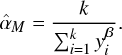 \begin{equation*}\hat{\alpha}_{M}=\frac{k}{\sum_{i=1}^{k}y_{i}^{\beta}}.\end{equation*}
Proof. Take the first derivative of (6) with respect to α and set to be zero, then we get
 \begin{align*}
\frac{\partial\log L_{2}(\alpha, \beta \mid \text {data})}{\partial\alpha}=\frac{k}{\alpha}-\sum_{i=1}^{k} y_{i}^{\beta}=0.
\end{align*}
 Then, we obtain  $\hat{\alpha}_{M}=\frac{k}{\sum_{i=1}^{k}y_{i}^{\beta}}.$
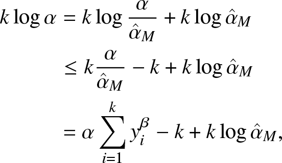
In the following, we prove the existence of the MLE of α. Let k ≠ 0 and β > 0 be fixed. Note that ![]() $\log t\le t-1$ for
$\log t\le t-1$ for ![]() $t=\frac{\alpha}{\hat{\alpha}_{M}}$, thus we have
$t=\frac{\alpha}{\hat{\alpha}_{M}}$, thus we have
 \begin{align*}
k\log \alpha& =k \log \frac{\alpha}{\hat{\alpha}_{M}}+k \log \hat{\alpha}_{M} \\
& \leq k \frac{\alpha}{\hat{\alpha}_{M}}-k+k \log \hat{\alpha}_{M} \\
& =\alpha\sum_{i=1}^{k}y_{i}^{\beta}-k+k \log \hat{\alpha}_{M} ,
\end{align*}
\begin{align*}
k\log \alpha& =k \log \frac{\alpha}{\hat{\alpha}_{M}}+k \log \hat{\alpha}_{M} \\
& \leq k \frac{\alpha}{\hat{\alpha}_{M}}-k+k \log \hat{\alpha}_{M} \\
& =\alpha\sum_{i=1}^{k}y_{i}^{\beta}-k+k \log \hat{\alpha}_{M} ,
\end{align*}which implies that
 \begin{align*}
\log L_{2}(\alpha, \beta \mid \text {data}) & = k \log \alpha+k \log \beta+(\beta-1) \sum_{i=1}^{k} \log y_{i}-\alpha \sum_{i=1}^{k} y_{i}^{\beta}\\
& \leq \alpha\sum_{i=1}^{k}y_{i}^{\beta}-k+k \log \hat{\alpha}_{M}+k \log \beta+(\beta-1) \sum_{i=1}^{k} \log y_{i}-\alpha \sum_{i=1}^{k} y_{i}^{\beta}\\
& =k \log \hat{\alpha}_{M}+k \log \beta+(\beta-1) \sum_{i=1}^{k} \log y_{i}-k.
\end{align*}
 Let  $ k=\hat{\alpha}_{M}\sum_{i=1}^{k}y_{i}^{\beta}$, then we further have
 \begin{align*}
\log L_{2}(\alpha, \beta \mid \text {data}) &\leq k \log \hat{\alpha}_{M}+k\log \beta+(\beta-1) \sum_{i=1}^{k} \log y_{i}-\hat{\alpha}_{M}\sum_{i=1}^{k}y_{i}^{\beta}\\
&=\log L_{2}(\hat{\alpha}_{M}, \beta \mid \text {data}).
\end{align*}
 The equation holds if and only if ![]() $\alpha = \hat{\alpha}_{M}$. This proves the assertion.
$\alpha = \hat{\alpha}_{M}$. This proves the assertion.
Theorem 3.4. The MLE of β exists and is unique which is the solution of
 \begin{align}
H(\beta)=\frac{k}{\beta}+\sum_{i=1}^{k}\log y_{i}-\alpha\sum_{i=1}^{k} y_{i}^{\beta}\log y_{i} =0.
\end{align}
\begin{align}
H(\beta)=\frac{k}{\beta}+\sum_{i=1}^{k}\log y_{i}-\alpha\sum_{i=1}^{k} y_{i}^{\beta}\log y_{i} =0.
\end{align}Proof. By computing the first partial derivative of (6) in regard to β, and set to be zero, (9) is obtained.
In (9), for convenience, let  $ H_{1}(\beta)=\sum_{i=1}^{k}\log y_{i}-\alpha\sum_{i=1}^{k} y_{i}^{\beta}\log y_{i}$. Then it is easy to figure out $\lim _{\beta \rightarrow 0^{+}} \frac{k}{\beta}=+\infty$ and
 ![]() $\lim _{\beta \rightarrow 0^{+}} H_{1}(\beta)$ is a constant, hence
$\lim _{\beta \rightarrow 0^{+}} H_{1}(\beta)$ is a constant, hence ![]() $\lim _{\beta \rightarrow 0^{+}} H(\beta)$
$\lim _{\beta \rightarrow 0^{+}} H(\beta)$ ![]() $=+\infty$.
$=+\infty$.
Note that,  $\lim _{\beta \rightarrow+\infty} \frac{m}{\beta}=0$. With regard to
 ![]() $\lim _{\beta \rightarrow+\infty} H_{1}(\beta)$, we divide yi into two parts, one is greater than 1 and the left is less than 1, because
$\lim _{\beta \rightarrow+\infty} H_{1}(\beta)$, we divide yi into two parts, one is greater than 1 and the left is less than 1, because  $\lim _{\beta \rightarrow+\infty} y_{i}^{\beta}=0$ for
 ![]() $y_{i} \lt 1$,
$y_{i} \lt 1$,  $\lim _{\beta \rightarrow+\infty} y_{i}^{\beta}=1$ for
 ![]() $y_{i}=1$, and
$y_{i}=1$, and  $\lim _{\beta \rightarrow+\infty} y_{i}^{\beta}=+\infty$ for
 ![]() $y_{i} \gt 1$. Then we can obtain that
$y_{i} \gt 1$. Then we can obtain that ![]() $\lim _{\beta \rightarrow+\infty} H_{1}(\beta) \lt 0$, then we have
$\lim _{\beta \rightarrow+\infty} H_{1}(\beta) \lt 0$, then we have ![]() $\lim _{\beta \rightarrow+\infty} H(\beta) \lt 0$.
$\lim _{\beta \rightarrow+\infty} H(\beta) \lt 0$.
Furthermore, since
 \begin{align*}
\frac{\mathrm d H(\beta)}{\mathrm d \beta}=-\frac{k}{\beta^{2}}-\alpha\sum_{i=1}^{k} y_{i}^{\beta}\left(\log y_{i}\right)^{2} \lt 0,
\end{align*}
 thus function ![]() $H(\beta)$ is decreasing from positive to negative. Hence, existence and uniqueness are proved.
$H(\beta)$ is decreasing from positive to negative. Hence, existence and uniqueness are proved.
As the dimensionality of the copula increases, the computation complexity of MLE also intensifies, rendering it impractical when dealing with a large number of parameters [Reference Joe17]. In order to overcome this hurdle, the two-step MLE is used as a favorable attractive alternative to the full MLE strategy, which is first proposed by [Reference Shih and Thomas29] for the two-dimensional case. In the first step, the MLEs ![]() $\hat{\lambda}_{M}, \hat{\delta}_{M}, \hat{\alpha}_{M}, \hat{\beta}_{M}$ are calculated by using nonlinear computational techniques such as the Newton-Raphson iteration approach. In the second step, the MLE of the dependence parameter θ in (1) is determined by constructing the following log-likelihood function based on the observed samples
$\hat{\lambda}_{M}, \hat{\delta}_{M}, \hat{\alpha}_{M}, \hat{\beta}_{M}$ are calculated by using nonlinear computational techniques such as the Newton-Raphson iteration approach. In the second step, the MLE of the dependence parameter θ in (1) is determined by constructing the following log-likelihood function based on the observed samples ![]() $\left(Z_{i}, Y_{i}\right)$,
$\left(Z_{i}, Y_{i}\right)$,
 \begin{align*}
\;\;\;\;\log L_{3}(\theta \mid \text {data})
&=\sum_{i=1}^{k} \log c(u_{i},v_{i};\theta)\\
&=k\log (1+\theta)-(1+\theta)\sum_{i=1}^{k}\log u_{i}v_{i}-(2+\frac{1}{\theta})\sum_{i=1}^{k}\log (u_{i}^{-\theta }+v_{i}^{-\theta }-1),
\end{align*}
 where c is density function of Clayton copula (1), ![]() $u_{i}=F_{Z}(z_{i};\hat{\lambda}_{M},\hat{\delta}_{M})$,
$u_{i}=F_{Z}(z_{i};\hat{\lambda}_{M},\hat{\delta}_{M})$, ![]() $v_{i}=G(y_{i};\hat{\alpha}_{M},\hat{\beta}_{M})$. By making the first derivatives of
$v_{i}=G(y_{i};\hat{\alpha}_{M},\hat{\beta}_{M})$. By making the first derivatives of ![]() $\log L_{3}(\theta \mid \text {data})$ with respect to θ to zero, the likelihood equation can be obtained as
$\log L_{3}(\theta \mid \text {data})$ with respect to θ to zero, the likelihood equation can be obtained as
 \begin{align*}
\frac{\mathrm d\log L_{3}(\theta \mid \text {data})}{\mathrm d\theta}=&
\frac{k}{1+\theta}-\sum_{i=1}^{k}\log u_{i}v_{i}+\frac{1}{\theta^2}\sum_{i=1}^{k}\log (u_{i}^{-\theta }+v_{i}^{-\theta }-1)\\
&+(2+\frac{1}{\theta})\sum_{i=1}^{k}\frac{u_{i}^{-\theta }\log u_{i}+v_{i}^{-\theta }\log v_{i}}{u_{i}^{-\theta }+v_{i}^{-\theta }-1}=0.
\end{align*}
 The estimated value ![]() $\hat{\theta}_{M}$ of θ can be gained by using optimization techniques.
$\hat{\theta}_{M}$ of θ can be gained by using optimization techniques.
Therefore, by substituting ![]() $\lambda, \delta, \alpha, \beta, \theta$ for
$\lambda, \delta, \alpha, \beta, \theta$ for ![]() $\hat{\lambda}_{M}, \hat{\delta}_{M}, \hat{\alpha}_{M}, \hat{\beta}_{M}, \hat{\theta}_{M}$ into (4), the MLE
$\hat{\lambda}_{M}, \hat{\delta}_{M}, \hat{\alpha}_{M}, \hat{\beta}_{M}, \hat{\theta}_{M}$ into (4), the MLE ![]() $\hat{R}_{M}$ of R may be produced by applying the MLE’s invariance property. Moreover, the
$\hat{R}_{M}$ of R may be produced by applying the MLE’s invariance property. Moreover, the ![]() $\mathrm{ACIs}$ of
$\mathrm{ACIs}$ of ![]() $\lambda, \delta, \alpha, \beta, \theta$ and R can be determined by leveraging the asymptotic normality of the MLEs.
$\lambda, \delta, \alpha, \beta, \theta$ and R can be determined by leveraging the asymptotic normality of the MLEs.
3.2. MPS estimation
Cheng and Amin [Reference Cheng and Amin10] introduced the MPS method, which provides an alternative way to estimate the parameters of a statistical model, especially when the MLE approach is impractical or computationally intensive. In our study, suppose that ![]() $z_{1: k} \lt z_{2: k} \lt \dots \lt z_{k: k}$ and
$z_{1: k} \lt z_{2: k} \lt \dots \lt z_{k: k}$ and ![]() $ y_{1: k} \lt y_{2: k} \lt \dots \lt y_{k: k}$ are the order sample of
$ y_{1: k} \lt y_{2: k} \lt \dots \lt y_{k: k}$ are the order sample of ![]() $z_{1}, z_{2}, \dots,z_{k}$ and
$z_{1}, z_{2}, \dots,z_{k}$ and ![]() $y_{1}, y_{2}, \dots,y_{k}$, respectively, and the corresponding uniform spacings can be given by
$y_{1}, y_{2}, \dots,y_{k}$, respectively, and the corresponding uniform spacings can be given by
and
where ![]() $i=1,2, \ldots, k+1, F_{Z}\left(z_{0: k} ; \lambda, \delta\right)=G\left(y_{0: k} ; \alpha, \beta\right)=0$ and
$i=1,2, \ldots, k+1, F_{Z}\left(z_{0: k} ; \lambda, \delta\right)=G\left(y_{0: k} ; \alpha, \beta\right)=0$ and ![]() $F_{Z}\left(z_{k+1: k} ; \lambda, \delta\right)=G\left(y_{k+1: k} ; \alpha, \beta\right)$ = 1. Then the MPS estimators
$F_{Z}\left(z_{k+1: k} ; \lambda, \delta\right)=G\left(y_{k+1: k} ; \alpha, \beta\right)$ = 1. Then the MPS estimators ![]() $\tilde{\lambda}_{P}, \tilde{\delta}_{P}, \tilde{\alpha}_{P}, \tilde{\beta}_{P}$ of
$\tilde{\lambda}_{P}, \tilde{\delta}_{P}, \tilde{\alpha}_{P}, \tilde{\beta}_{P}$ of ![]() $\lambda, \delta, \alpha,\beta$ can be obtained in the first step by maximizing
$\lambda, \delta, \alpha,\beta$ can be obtained in the first step by maximizing
 \begin{equation*}
M_{1}(\lambda, \delta)=\frac{1}{k+1} \sum_{i=1}^{k+1} \log \left( D_{1 i}(\lambda, \delta)\right)
\end{equation*}
\begin{equation*}
M_{1}(\lambda, \delta)=\frac{1}{k+1} \sum_{i=1}^{k+1} \log \left( D_{1 i}(\lambda, \delta)\right)
\end{equation*}and
 \begin{equation*}
M_{2}(\alpha, \beta)=\frac{1}{k+1} \sum_{i=1}^{k+1} \log \left(D_{2 i}(\alpha, \beta)\right)
\end{equation*}
 with respect to ![]() $\lambda, \delta$ and
$\lambda, \delta$ and ![]() $ \alpha, \beta$, respectively. Further, define
$ \alpha, \beta$, respectively. Further, define
 \begin{align*}
D_{3 i}(\theta)=C\left(F_{Z}(z_{i: k}; \tilde{\lambda}_{P}, \tilde{\delta}_{P} ), G(y_{i: k} ; \tilde{\alpha}_{P}, \tilde{\beta}_{P}) ; \theta\right)-C\left(F_{Z}(z_{i-1: k}; \tilde{\lambda}_{P}, \tilde{\delta}_{P} ), G(y_{i-1: k} ; \tilde{\alpha}_{P}, \tilde{\beta}_{P}) ; \theta\right).
\end{align*}
 Following the idea in the first step, then the MPS estimator ![]() $\tilde{\theta}_{P}$ of θ can be obtained by maximizing
$\tilde{\theta}_{P}$ of θ can be obtained by maximizing
 \begin{align*}
M_{3}(\theta)=&\frac{1}{k+1} \sum_{i=1}^{k+1} \log D_{3 i}(\theta)
\end{align*}
\begin{align*}
M_{3}(\theta)=&\frac{1}{k+1} \sum_{i=1}^{k+1} \log D_{3 i}(\theta)
\end{align*}with respect to θ.
Therefore, substituting the MPS estimators for λ, δ, α, β and θ into Eq. (4), and the MPS estimation ![]() $\tilde{R}_{P}$ of R then can be computed by applying the MPS estimator’s invariance property.
$\tilde{R}_{P}$ of R then can be computed by applying the MPS estimator’s invariance property.
4. Bootstrap confidence intervals
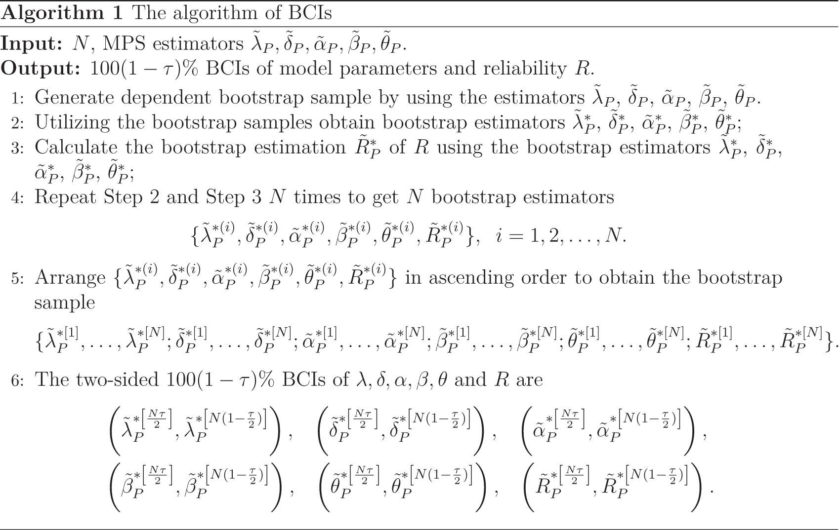
On the one hand, the assumption of asymptotic normality relies on large sample sizes and is based on the theory of large samples. However, in certain cases, the available sample sizes are very small. The bootstrap methods prove to be more suitable and reliable for constructing CIs in such situations. On the other hand, while the MPS estimator of R can be obtained using the MPS method, constructing ![]() $\mathrm{CIs}$ for unknown parameters and R is not straightforward. In such cases, the parametric bootstrap percentile method is employed to construct bootstrap confidence intervals (BCIs) for unknown parameters and R based on MPS estimators. Following is the specific Algorithm 1.
$\mathrm{CIs}$ for unknown parameters and R is not straightforward. In such cases, the parametric bootstrap percentile method is employed to construct bootstrap confidence intervals (BCIs) for unknown parameters and R based on MPS estimators. Following is the specific Algorithm 1.
5. Simulation study
This section illustrates the inference methods described in the previous sections by conducting Monte Carlo simulation. Consider a 3-1 parallel-series system in the multicomponent stress–strength model, that is ![]() $(m, n)=(3,1)$. We take λ = 0.2, δ = 3.6, α = 0.5, β = 0.7. For given dependence parameters θ = 2, θ = 2.5, and θ = 3, the respective true values of R are 0.149550, 0.141699, and 0.135706.
$(m, n)=(3,1)$. We take λ = 0.2, δ = 3.6, α = 0.5, β = 0.7. For given dependence parameters θ = 2, θ = 2.5, and θ = 3, the respective true values of R are 0.149550, 0.141699, and 0.135706.
Suppose that the dependent sample ![]() $\left({z}, {y}\right)$ derived from Clayton copula
$\left({z}, {y}\right)$ derived from Clayton copula ![]() $C(u, v)$ denotes
$C(u, v)$ denotes  $c_{u}(v)=\frac{\partial C(u, v)}{\partial u}$. The next Algorithm 2 is employed to generate the dependent samples.

Using the generated dependent samples, we employ the two-step MLE and MPS methods to estimate the model parameters. The average estimators, Biases, mean square errors (MSEs), ![]() $\mathrm{CIs}$, and
$\mathrm{CIs}$, and ![]() $\mathrm{CI}$ lengths of the unknown parameters are computed based on 1,000 times simulation. The simulation results are presented in Tables 1–6.
$\mathrm{CI}$ lengths of the unknown parameters are computed based on 1,000 times simulation. The simulation results are presented in Tables 1–6.
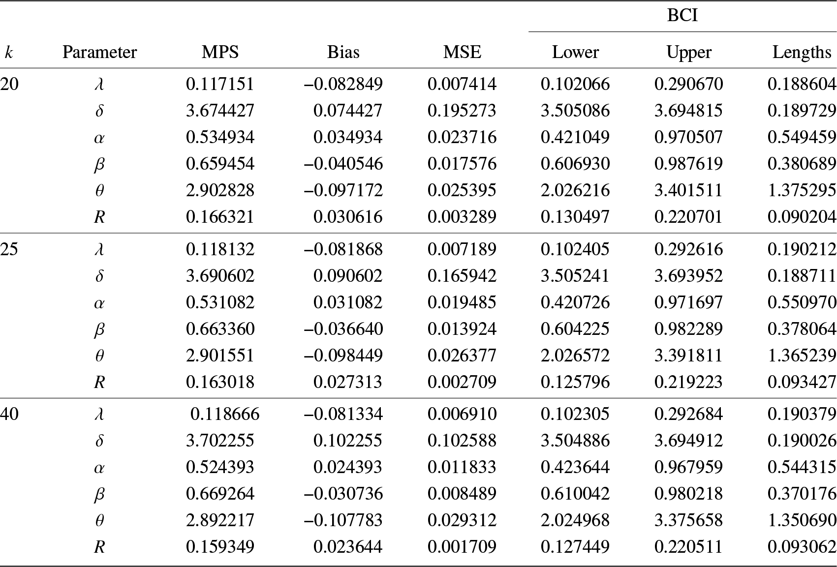
From Tables 1–6, some conclusions could be found.
(i) The Biases and MSEs of both MLEs and MPS estimators of model parameters present a downward trend as the value of k increases. This indicates that the estimations become more accurate with higher values of k.
(ii) For the majority of circumstances, as k rises, so do the biases of the MLEs of the dependence parameter and R. Because the MLEs of the dependence parameter and R are computed using the MLEs of the model parameters, the error is compounding as the sample size increases.
(iii) When the dependency parameter takes on different values, the biases of the estimators for both the model parameters and ![]() $ R $ show no significant change for the same sample size.
$ R $ show no significant change for the same sample size.
(iv) The length of the intervals tends to decrease with an increase in k. The interval lengths of BCIs are shorter when k is small, whereas the interval lengths of MLEs are shorter when k is larger.
(v) It is worth mentioning that in the context of R, although there is only a small difference between the MLEs and MPS estimators, it can be observed that the MLE performs slightly better than the MPS.
Table 1. MLEs, biases, MSEs, and ACIs for ![]() $\lambda, \delta, \alpha ,\beta,\theta$, and R (θ = 2).
$\lambda, \delta, \alpha ,\beta,\theta$, and R (θ = 2).
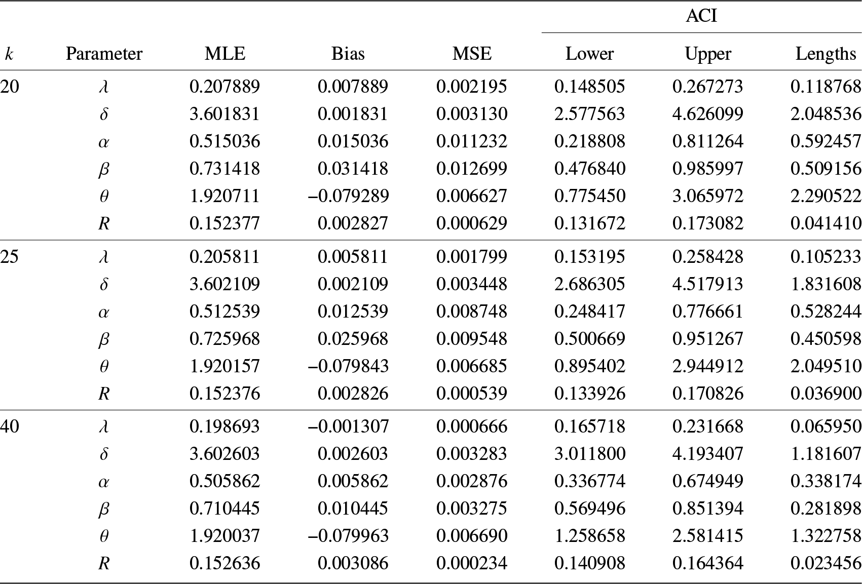
Table 2. MPSs, biases, MSEs, and BCIs for ![]() $\lambda,\delta, \alpha ,\beta,\theta$, and R (θ = 2).
$\lambda,\delta, \alpha ,\beta,\theta$, and R (θ = 2).
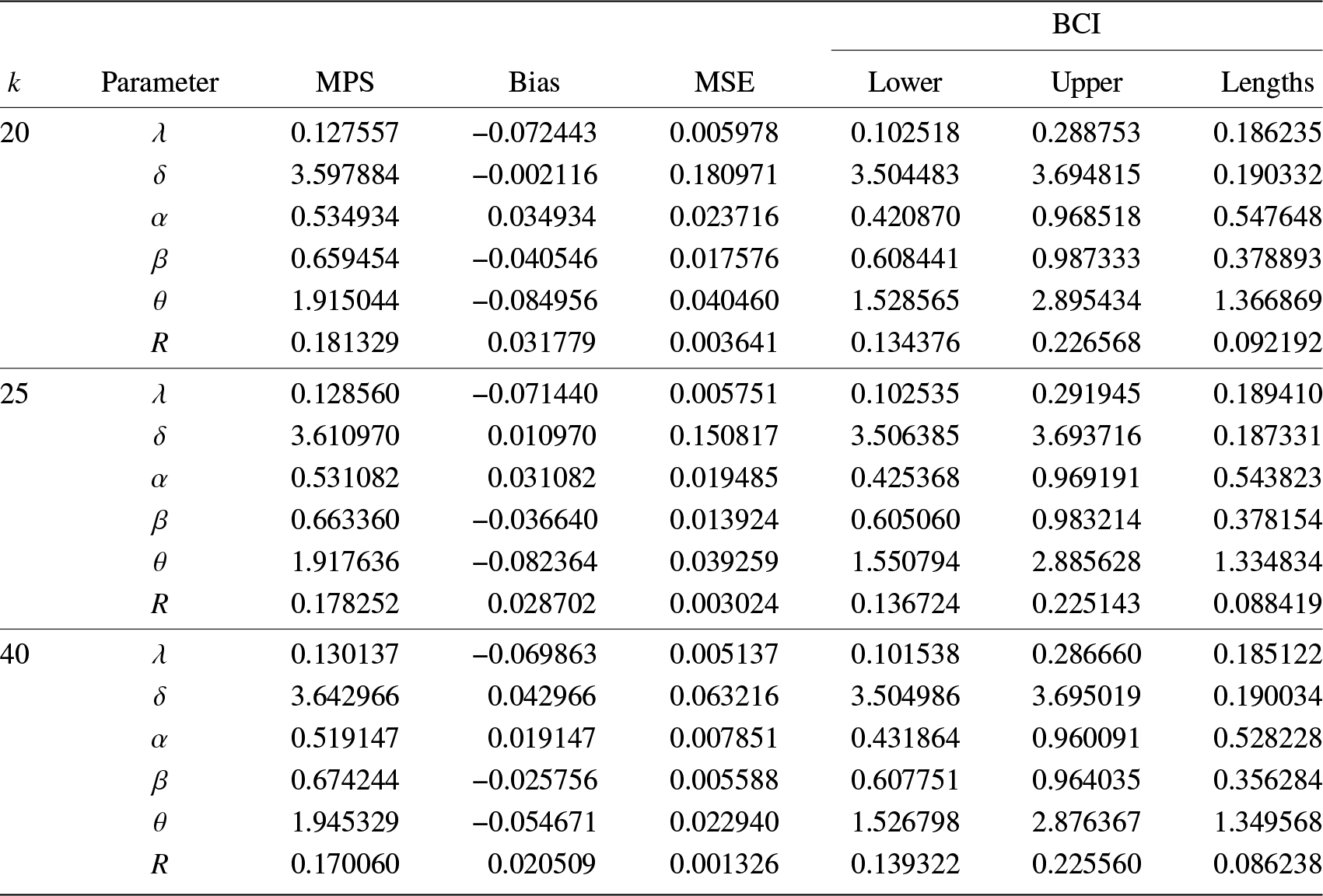
Table 3. MLEs, biases, MSEs, and ACIs for ![]() $\lambda,\delta,\alpha ,\beta,\theta$, and R (θ = 2.5).
$\lambda,\delta,\alpha ,\beta,\theta$, and R (θ = 2.5).
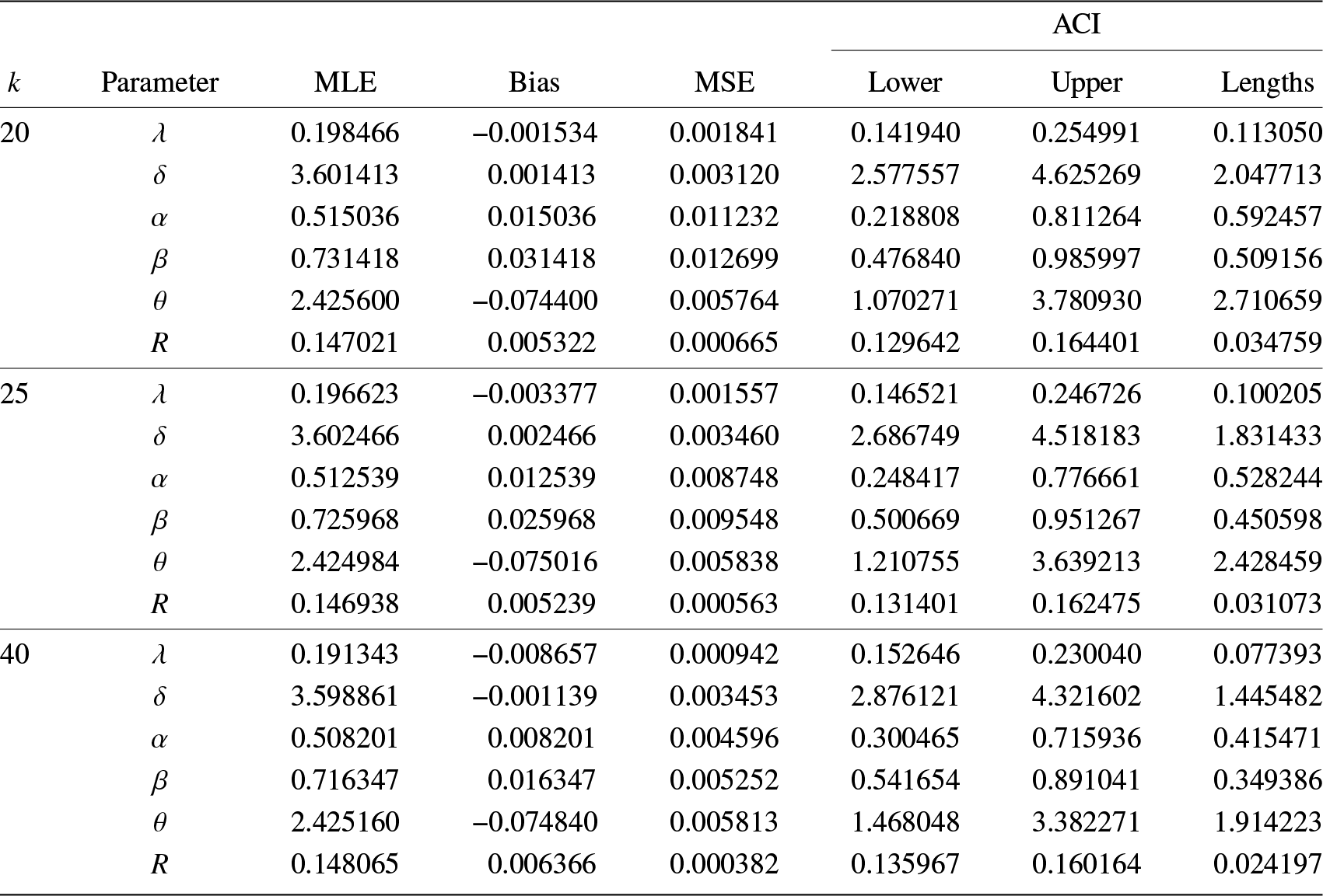
Table 4. MPSs, biases, MSEs, and BCIs for ![]() $\lambda,\delta,\alpha,\beta,\theta$, and R (θ = 2.5).
$\lambda,\delta,\alpha,\beta,\theta$, and R (θ = 2.5).
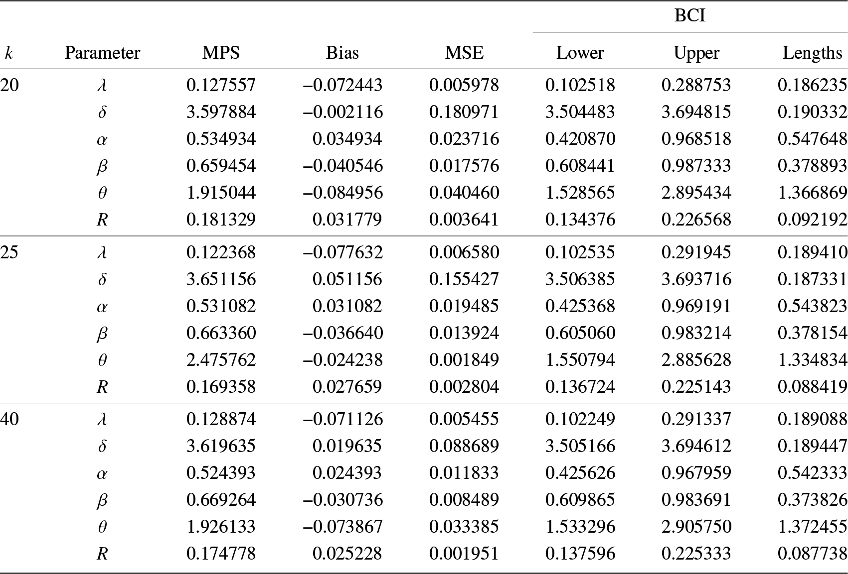
Table 5. MLEs, biases, MSEs, and ACIs for ![]() $\lambda,\delta,\alpha ,\beta,\theta$, and R (θ = 3).
$\lambda,\delta,\alpha ,\beta,\theta$, and R (θ = 3).
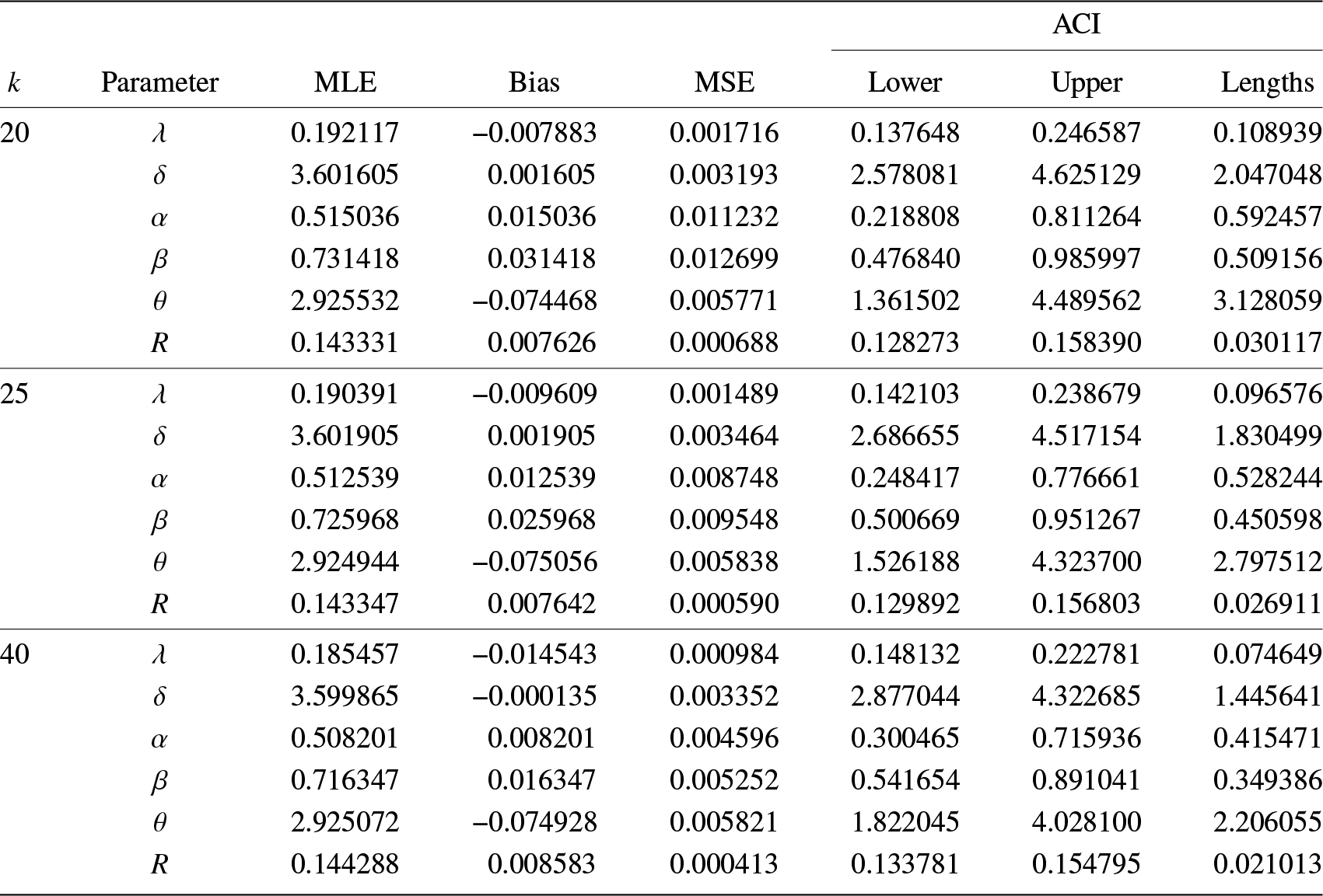
Table 6. MPSs, biases, MSEs, and BCIs for ![]() $\lambda,\delta,\alpha,\beta,\theta$, and R (θ = 3).
$\lambda,\delta,\alpha,\beta,\theta$, and R (θ = 3).
6. Real data analysis
In the following, we analyze two real datasets and present the practical applicability of the aforementioned methods. We consider datasets, from two groups of patients suffering from head and neck cancer disease. Both of these datasets were analyzed and discussed in the context of stress–strength reliability analysis by [Reference Bai, Li, Balakrishnan and He5]. Now, we give the application of our established model to analyze the two real datasets, which are listed as follows:
Data 1: 12.20, 23.56, 23.74, 25.87, 31.98, 37, 41.35, 47.38, 55.46, 58.36, 63.47, 68.46, 74.48, 78.26, 81.43, 84, 92, 94, 110, 112, 119, 127, 130, 133, 140, 146, 155, 159, 173, 179, 194, 195, 209, 249, 281, 319, 339, 432, 469, 519, 633, 725, 817, 1,776.
Data 2: 6.53, 7, 10.42, 14.48, 16.10, 22.70, 34, 41.55, 42, 45.28, 49.40, 53.62, 63, 83, 84, 91, 108, 112, 129, 133, 133, 139, 140, 140, 146, 149, 154, 157, 160, 160, 165, 173, 176, 218, 225, 241, 248, 273, 277, 297, 405, 417, 420, 440, 523, 583, 594, 1,101, 1,146, 1,417.
To enhance the efficiency of dependency analysis, it is important to maintain a consistent sample size across both datasets. Using the sample function in R, we randomly selected a subset of Data 2 (designated as Data 2*) to match the sample size of Data 1, which represents strength data, while Data 2* represents stress data.
Data 2*: 14.48 , 176, 6.53, 157,108, 248, 41.55, 53.62, 154, 84, 405, 241, 11,14, 12, 42, 297, 165, 129., 1,146, 594, 173, 225, 417, 83, 10.42, 15, 273, 140, 140, 160, 149, 160, 22.7, 133, 13, 583, 91, 523, 139, 63, 218, 440, 7.
To model the dependence between strength and stress, we chose the Clayton copula for its ability to capture lower tail dependence, which is particularly relevant in reliability data where simultaneous low values (e.g., stress and strength failures) are of interest [Reference Nelsen27]. Although other copulas like the Gumbel and Frank are also used in reliability studies, the Clayton copula better matched our data’s dependence structure. We also evaluated the Gumbel and Frank copulas. A goodness-of-fit test, shown in Table 7, yielded a high p-value (0.8861) for the Clayton copula, where the significance of the bold value indicates the optimal result, confirming its suitability for modeling the observed dependence. Future research might explore nonparametric approaches, such as empirical copulas or kernel-based estimations, to capture more complex dependence structures.
Table 7. Goodness-of-fit test results for copula.

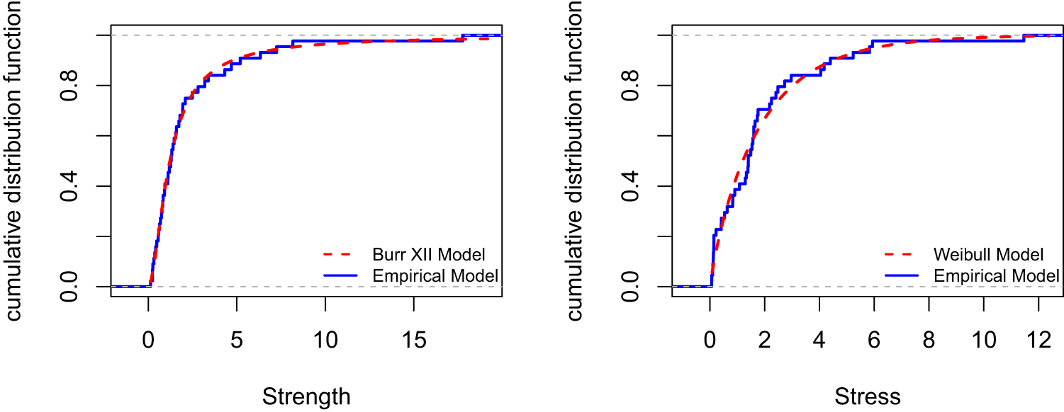
Figure 2. Empirical model and the fitted model of real datasets.
Through iterative procedures, we can obtain the MLE and MPS estimator of λ are ![]() $\hat \lambda_{M}=1.8619$ and
$\hat \lambda_{M}=1.8619$ and ![]() $\tilde \lambda_{P}=1.7211$, the MLE and MPS estimator of δ are
$\tilde \lambda_{P}=1.7211$, the MLE and MPS estimator of δ are ![]() $\hat \delta_{M}=0.7774$ and
$\hat \delta_{M}=0.7774$ and ![]() $\tilde \delta_{P}=0.7824$, the MLE and MPS estimator of α are
$\tilde \delta_{P}=0.7824$, the MLE and MPS estimator of α are ![]() $\hat\alpha_{M}=0.5870$ and
$\hat\alpha_{M}=0.5870$ and ![]() $\tilde\alpha_{P}=0.6105$, the MLE and MPS estimator of β are
$\tilde\alpha_{P}=0.6105$, the MLE and MPS estimator of β are ![]() $\hat\beta_{M}=0.9093$ and
$\hat\beta_{M}=0.9093$ and ![]() $\tilde\beta_{P}=0.8201$, the MLE and MPS estimator of θ are
$\tilde\beta_{P}=0.8201$, the MLE and MPS estimator of θ are ![]() $\hat\theta_{M}=0.2422$ and
$\hat\theta_{M}=0.2422$ and ![]() $\tilde\theta_{P}=0.2499$. Using the above datasets, the MLE and MPS estimator for system reliability are
$\tilde\theta_{P}=0.2499$. Using the above datasets, the MLE and MPS estimator for system reliability are ![]() $\hat R_{M}=0.5378$ and
$\hat R_{M}=0.5378$ and ![]() $\tilde R_{P}=0.5468$.
$\tilde R_{P}=0.5468$.
In order to determine the suitability of the Burr XII and Weibull distributions for fitting the datasets, we utilize the computed estimators of unknown parameters to calculate the Kolmogorov–Smirnov (K-S) test statistic and corresponding p-values. For strength data, the K-S statistic for the Burr XII model is D = 0.0480 with a p-value of p = 0.9998. For stress data, the K-S statistic for the Weibull model is D = 0.1138 with a p-value of p = 0.6188. The empirical distribution curves based on data 1 and data 2*, along with the fitted Burr XII and Weibull marginal distribution curves for strength and stress, are presented in Figure 2. These results indicate that both models provide an excellent fit for the respective datasets.
7. Conclusion
This paper investigated the estimation of reliability for a multicomponent parallel-series system while considering the presence of dependence between stress and strength based on Clayton copula. We employed the two-step MLE and MPS approaches to estimate the system reliability, assuming Weibull and Burr XII distributions for stress and strength, respectively. The simulation results demonstrate that the two-step MLE method outperformed the MPS method in terms of reliability estimation. Real data analysis gives the applicability of the presented results. Although this study successfully addressed the reliability estimation problem, one important aspect that remains unexplored is the selection of an appropriate copula, which is of interest to pursue.
Acknowledgments
The authors acknowledge the supports of the National Natural Science Foundation of China (No. 12361060), the Industrial Support Program of Gansu Provincial Education Department (No. 2025CYZC-016), the Science and Technology Program of Gansu Province (No. 24JRRA144), and College Teachers Innovation Foundation Project of Gansu Provincial Education Department (No. 2024A-002).
Conflict of interest
The authors declare that they have no conflict of interest.


