


Introduction
The classification of simple Lie algebras over algebraically closed fields is a classical subject, and the situation is, in many aspects, well understood. That is not the case at all over arbitrary fields. Typically, this situation is studied by first extending to a splitting field (e.g., the algebraic closure) and then performing Galois descent, using tools such as Galois cohomology.
This is not the only possible approach, however. Inspired by the successful applications (e.g., by Efim Zel’manov and Alekseĭ Kostrikin [Reference Zelmanov and KostrikinZK90]) of sandwich elements (i.e., nonzero elements x in a Lie algebra L such that $\operatorname {\mathrm {ad}}_x^2 = 0$
), various people have studied simple Lie algebras through the concept of extremal elements. A nonzero element
$\operatorname {\mathrm {ad}}_x^2 = 0$
), various people have studied simple Lie algebras through the concept of extremal elements. A nonzero element $x \in L$
is called extremal if
$x \in L$
is called extremal if $[x, [x, L]] \leq kx$
(together with an additional axiom that is relevant only in characteristic
$[x, [x, L]] \leq kx$
(together with an additional axiom that is relevant only in characteristic $2$
); notice that this implies
$2$
); notice that this implies $\operatorname {\mathrm {ad}}_x^3 = 0$
. A typical example of an extremal element is a long root element in a classical Lie algebra. In fact, these extremal elements span a one-dimensional inner ideal of the Lie algebra, a notion going back to John Faulkner [Reference FaulknerFau73] and Georgia Benkart [Reference BenkartBen74]. The first paper explicitly underlying the importance of one-dimensional inner ideals, that we are aware of, is Alexander Premet’s paper [Reference PremetPre86] from 1986; see, in particular, its main result stating that any finite-dimensional Lie algebra over an algebraically closed field of characteristic
$\operatorname {\mathrm {ad}}_x^3 = 0$
. A typical example of an extremal element is a long root element in a classical Lie algebra. In fact, these extremal elements span a one-dimensional inner ideal of the Lie algebra, a notion going back to John Faulkner [Reference FaulknerFau73] and Georgia Benkart [Reference BenkartBen74]. The first paper explicitly underlying the importance of one-dimensional inner ideals, that we are aware of, is Alexander Premet’s paper [Reference PremetPre86] from 1986; see, in particular, its main result stating that any finite-dimensional Lie algebra over an algebraically closed field of characteristic $p>5$
contains a one-dimensional inner ideal (Theorem 1). The idea of extremal elements has also famously been used by Vladimir Chernousov in his proof of the Hasse principle for algebraic groups of type
$p>5$
contains a one-dimensional inner ideal (Theorem 1). The idea of extremal elements has also famously been used by Vladimir Chernousov in his proof of the Hasse principle for algebraic groups of type $E_8$
[Reference ChernousovChe89]. (He called the extremal elements root elements because in his situation, they belong to root groups. A detailed exposition can be found in [Reference Platonov and RapinchukPR94, Chapter 6, Section 8]; see, in particular, the discussion about root elements starting on p. 387.)
$E_8$
[Reference ChernousovChe89]. (He called the extremal elements root elements because in his situation, they belong to root groups. A detailed exposition can be found in [Reference Platonov and RapinchukPR94, Chapter 6, Section 8]; see, in particular, the discussion about root elements starting on p. 387.)
Around the turn of the century, Arjeh Cohen and his collaborators (Anja Steinbach, Rosane Ushirobira, David Wales, Gábor Ivanyos, Dan Roozemond) obtained the clever insight that the extremal elements have a geometric interpretation, and the corresponding one-dimensional inner ideals can serve as the point set of a so-called shadow space of a building [Reference Cohen, Steinbach, Ushirobira and WalesCSUW01, Reference Cohen and IvanyosCI06, Reference Cohen and IvanyosCI07, Reference Cohen, Ivanyos and RoozemondCIR08]. That idea led them to the notion of a root filtration space and makes it possible to visualize the different relations between extremal elements. In particular, distinct extremal points can be in four possible relations: collinear, symplectic, special or hyperbolic. These notions will play an important role in Sections 2 and 3 of our paper. In particular, a crucial ingredient will be the result by Cohen and Ivanyos that each hyperbolic pair of extremal points gives rise to a $5$
-grading of the Lie algebra.
$5$
-grading of the Lie algebra.
Since then, extremal elements in Lie algebras, and the corresponding extremal geometry, have been studied by various people; see, for instance, [Reference Draisma and in ’t panhuisDitp08, Reference in ’t panhuis, Postma and RoozemonditpPR09, Reference RoozemondRoo11, Reference CohenCoh12, Reference Cuypers, Roberts and ShpectorovCRS15, Reference LópezFL16, Reference Cuypers and FleischmannCF18, Reference Cuypers and MeulewaeterCM21, Reference Cuypers and FleischmannCF23] and [Reference LópezFL19, Chapter 6]. The origin of the terminology ‘extremal elements’ remains slightly mysterious. We have learned from Arjeh Cohen that he believes that he picked it up from Jean-Pierre Serre and consequently used it in their paper [Reference Cohen, Steinbach, Ushirobira and WalesCSUW01], but neither Cohen nor we have been able to find a written source confirming this origin, and in fact, Serre informed us that he does not think that he is responsible for this terminology, but ‘that it is possible that [he] used it once in a discussion’.
In our paper, we will adopt a different point of view on extremal elements and relate the Lie algebras to two types of exceptional algebraic structures: cubic norm structures and quadrangular algebras.
Cubic norm structures are well known: The Book of Involutions [Reference Knus, Merkurjev, Rost and TignolKMRT98] spends a whole Chapter IX on them. In particular, §38 and the Notes at the end of Chapter IX contain a lot of additional information and (historical) background. The key players in this theory are Hans Freudenthal [Reference FreudenthalFre54], Tonny Springer [Reference SpringerSpr62], Kevin McCrimmon [Reference McCrimmonMcC69], Holger Petersson and Michel Racine [Reference Petersson and RacinePR84, Reference Petersson and RacinePR86a, Reference Petersson and RacinePR86b]. We will also encounter ‘twin cubic norm structures’ (or ‘cubic norm pairs’), a notion that seems to have appeared only once before in the literature in a paper by John Faulkner [Reference FaulknerFau01].
Quadrangular algebras are certainly not so well known. They first appeared implicitly in the work of Jacques Tits and Richard Weiss on the classification of Moufang polygons, which are geometric structures (spherical buildings of rank 2) associated to simple linear algebraic groups of relative rank 2 [Reference Tits and WeissTW02]. The first explicit definition of these algebras, in the anisotropic case, appeared in Weiss’ monograph [Reference WeissWei06]. The general definition of arbitrary quadrangular algebras is even more recent and is due to Bernhard Mühlherr and Richard Weiss [Reference Mühlherr and WeissMW19]. The definition looks rather daunting (see Definition 1.17 below) mostly because of technicalities in characteristic $2$
, although the definition itself is characteristic-free.
$2$
, although the definition itself is characteristic-free.
It is worth pointing out that the anisotropic quadrangular algebras are precisely the parametrizing structures for Moufang quadrangles and that the anisotropic cubic norm structures are precisely the parametrizing structures for Moufang hexagons. More generally, arbitrary quadrangular algebras and arbitrary cubic norm structures (which might or might not be anisotropic) have been used in the theory of Tits quadrangles and Tits hexagons, respectively [Reference Mühlherr and WeissMW22]. See, in particular, the appendix of [Reference Mühlherr and WeissMW19] for the connection between quadrangular algebras and Tits quadrangles, and [Reference Mühlherr and WeissMW22, Chapter 2] for the connection between cubic norm structures and Tits hexagons. Notice that Moufang quadrangles are, in fact, buildings of type $B_2$
or
$B_2$
or $BC_2$
, and that Moufang hexagons are buildings of type
$BC_2$
, and that Moufang hexagons are buildings of type $G_2$
. (In the language of linear algebraic groups, this is the type of the relative root system.)
$G_2$
. (In the language of linear algebraic groups, this is the type of the relative root system.)
In our approach, we will start from a simple Lie algebra admitting extremal elements satisfying two possible sets of assumptions (see Theorems B and C below). In each of these two cases, we will use two different hyperbolic pairs of extremal points, giving rise to two different $5$
-gradings on the Lie algebra, so we obtain a
$5$
-gradings on the Lie algebra, so we obtain a $5 \times 5$
-graded Lie algebra. Depending on which of the two cases we are considering, this
$5 \times 5$
-graded Lie algebra. Depending on which of the two cases we are considering, this $5 \times 5$
-grading takes a different shape. For the reader’s convenience, we have reproduced smaller versions of Figures 1 and 2 of these gradings below, that can be found in full size on pages 32 and 42, respectively.
$5 \times 5$
-grading takes a different shape. For the reader’s convenience, we have reproduced smaller versions of Figures 1 and 2 of these gradings below, that can be found in full size on pages 32 and 42, respectively.

A closer look at these gradings reveals that, in fact, the $5 \times 5$
-grading in Figure 1 is a
$5 \times 5$
-grading in Figure 1 is a $G_2$
-grading, and the
$G_2$
-grading, and the $5 \times 5$
-grading in Figure 2 is a
$5 \times 5$
-grading in Figure 2 is a $BC_2$
-grading. We will show that in the first case, the Lie algebra is parametrized by a cubic norm pair, in the sense that each of the pieces arising in the decomposition as well as the explicit formulas describing their Lie brackets, are determined by the structure of this cubic norm pair (Theorem B). In the second case, it turns out that the Lie algebra is parametrized by a quadrangular algebra (Theorem C).
$BC_2$
-grading. We will show that in the first case, the Lie algebra is parametrized by a cubic norm pair, in the sense that each of the pieces arising in the decomposition as well as the explicit formulas describing their Lie brackets, are determined by the structure of this cubic norm pair (Theorem B). In the second case, it turns out that the Lie algebra is parametrized by a quadrangular algebra (Theorem C).
The study of Lie algebras graded by root systems is not new, and we refer, for instance, to the work of Bruce Allison, Georgia Benkart, Yun Gao and Efim Zel’manov [Reference Allison, Benkart and GaoABG02, Reference Benkart and ZelmanovBZ96]. However, their goals have been rather different from ours. Whereas earlier research has focused on classifying all Lie algebras graded by certain root systems in terms of central extensions of TKK-constructions, we focus on simple Lie algebras, but we have as goal to understand the internal structure of the Lie algebra, via the different pieces of the grading, directly in terms of an algebraic structure.Footnote 1 In addition, we do not assume the existence of a $BC_2$
-or
$BC_2$
-or $G_2$
-grading, but it is a consequence of some natural conditions on the extremal elements of the Lie algebra. These conditions are satisfied very often, and in fact, there are many Lie algebras for which both sets of conditions are satisfied, and hence admit both a
$G_2$
-grading, but it is a consequence of some natural conditions on the extremal elements of the Lie algebra. These conditions are satisfied very often, and in fact, there are many Lie algebras for which both sets of conditions are satisfied, and hence admit both a $BC_2$
-and a
$BC_2$
-and a $G_2$
-grading, and hence, they can be parametrized both by a cubic norm structure and by a quadrangular algebra! It is our hope that this observation will lead to a deeper understanding of connections between different forms of exceptional Lie algebras (and exceptional algebraic groups, as well as their geometric counterparts – namely, the corresponding Moufang polygons and Tits polygons mentioned above). We have indicated a first impression in this direction in Remark 1.2 in the appendix.
$G_2$
-grading, and hence, they can be parametrized both by a cubic norm structure and by a quadrangular algebra! It is our hope that this observation will lead to a deeper understanding of connections between different forms of exceptional Lie algebras (and exceptional algebraic groups, as well as their geometric counterparts – namely, the corresponding Moufang polygons and Tits polygons mentioned above). We have indicated a first impression in this direction in Remark 1.2 in the appendix.
We formulate our main results. We emphasize that k is an arbitrary field of arbitrary characteristic.
Theorem A. Let L be a simple Lie algebra. Assume that for some Galois extension $k'/k$
with
$k'/k$
with $k'\neq \mathbb F_2$
,
$k'\neq \mathbb F_2$
, $L_{k'} := L \otimes _k k'$
is a simple Lie algebra generated by its pure extremal elements such that the extremal geometry contains lines.
$L_{k'} := L \otimes _k k'$
is a simple Lie algebra generated by its pure extremal elements such that the extremal geometry contains lines.
Consider a hyperbolic pair $(x,y)$
of extremal elements and let
$(x,y)$
of extremal elements and let $L=L_{-2}\oplus L_{-1}\oplus L_0\oplus L_1\oplus L_2$
be the associated
$L=L_{-2}\oplus L_{-1}\oplus L_0\oplus L_1\oplus L_2$
be the associated $5$
-grading.
$5$
-grading.
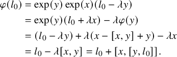
Then for each $l \in L_1$
, we can define an ‘l-exponential automorphism’
$l \in L_1$
, we can define an ‘l-exponential automorphism’
 $$\begin{align*}\alpha \colon L \to L \colon m \mapsto m+[l,m]+q_{\alpha}(m)+n_{\alpha}(m)+v_{\alpha}(m), \end{align*}$$
where $q_{\alpha },n_{\alpha },v_{\alpha } \colon L \to L$
are maps with
$q_{\alpha },n_{\alpha },v_{\alpha } \colon L \to L$
are maps with
 $$ \begin{align*} q_{\alpha}(L_i)\subseteq L_{i+2}, \quad n_{\alpha}(L_i)\subseteq L_{i+3}, \quad v_{\alpha}(L_i)\subseteq L_{i+4} \end{align*} $$
for all $i\in [-2,2]$
.
$i\in [-2,2]$
.
This is shown in Theorem 3.16 below, with the essential part being obtained by Theorem 3.13, along with uniqueness results and other auxiliary results. (Notice that $\alpha $
is not unique: there is a one-parameter family of such automorphisms.)
$\alpha $
is not unique: there is a one-parameter family of such automorphisms.)
In particular, when $\operatorname {\mathrm {char}}(k) \neq 2$
, we can always choose
$\operatorname {\mathrm {char}}(k) \neq 2$
, we can always choose $q_\alpha (m) = \tfrac {1}{2}[l, [l, m]]$
, and if, in addition,
$q_\alpha (m) = \tfrac {1}{2}[l, [l, m]]$
, and if, in addition, $\operatorname {\mathrm {char}}(k) \neq 3$
, then it is a consequence that
$\operatorname {\mathrm {char}}(k) \neq 3$
, then it is a consequence that $n_\alpha (m) = \tfrac {1}{6} [l, [l, [l, m]]]$
and that
$n_\alpha (m) = \tfrac {1}{6} [l, [l, [l, m]]]$
and that $v_\alpha (m) = \tfrac {1}{24} [l, [l, [l, [l, m]]]]$
, so our l-exponential automorphism really are a generalization of the usual exponential automorphisms.
$v_\alpha (m) = \tfrac {1}{24} [l, [l, [l, [l, m]]]]$
, so our l-exponential automorphism really are a generalization of the usual exponential automorphisms.
It is worth mentioning that the condition ‘being generated by pure extremal elements’ is easily fulfilled. For instance, the main result of [Reference Cohen, Ivanyos and RoozemondCIR08] shows that as soon as $\operatorname {\mathrm {char}}(k)> 5$
, each simple Lie algebra admitting a single pure extremal element is, in fact, generated by its extremal elements. (See also [Reference LópezFL19, Chapter 6].) However, there exist interesting simple Lie algebras not admitting any extremal element, and in that case, studying the minimal inner ideals instead is an interesting approach. We refer, for instance, to our earlier work [Reference De Medts and MeulewaeterDMM24] for examples of this situation.
$\operatorname {\mathrm {char}}(k)> 5$
, each simple Lie algebra admitting a single pure extremal element is, in fact, generated by its extremal elements. (See also [Reference LópezFL19, Chapter 6].) However, there exist interesting simple Lie algebras not admitting any extremal element, and in that case, studying the minimal inner ideals instead is an interesting approach. We refer, for instance, to our earlier work [Reference De Medts and MeulewaeterDMM24] for examples of this situation.
In addition, notice that the existence of a Galois extension $k'/k$
such that the extremal geometry of the Lie algebra over
$k'/k$
such that the extremal geometry of the Lie algebra over $k'$
contains lines, is also easily fulfilled. Indeed, if
$k'$
contains lines, is also easily fulfilled. Indeed, if $\operatorname {\mathrm {char}}(k) \neq 2$
, then it follows from [Reference Cuypers and FleischmannCF23, Theorem 1.1], and the paragraph following this result that unless the Lie algebra is a symplectic Lie algebra (i.e., of the form
$\operatorname {\mathrm {char}}(k) \neq 2$
, then it follows from [Reference Cuypers and FleischmannCF23, Theorem 1.1], and the paragraph following this result that unless the Lie algebra is a symplectic Lie algebra (i.e., of the form $\mathfrak {fsp}(V, f)$
for some nondegenerate symplectic space
$\mathfrak {fsp}(V, f)$
for some nondegenerate symplectic space $(V,f)$
), there always even exists an extension
$(V,f)$
), there always even exists an extension $k'/k$
of degree at most
$k'/k$
of degree at most $2$
fulfilling the requirement that the extremal geometry contains lines. (It is a more subtle fact that the simplicity of the Lie algebra is preserved after such a base extension, but we deal with this in Lemma 5.2.)
$2$
fulfilling the requirement that the extremal geometry contains lines. (It is a more subtle fact that the simplicity of the Lie algebra is preserved after such a base extension, but we deal with this in Lemma 5.2.)
Our Theorems B and C are very similar in structure. Notice the difference between the conditions between the two results. In Theorem B, the main condition is the fact that we require the existence of lines already over the base field k. In Theorem C, the main condition is the existence of a symplectic pair of extremal elements. (Notice that by the preceding discussion, condition (i) in the statement of Theorem C essentially only excludes symplectic Lie algebras.)
Theorem B. Let L be a simple Lie algebra defined over a field k with $|k| \geq 4$
. Assume that L is generated by its pure extremal elements and that the extremal geometry contains lines.
$|k| \geq 4$
. Assume that L is generated by its pure extremal elements and that the extremal geometry contains lines.
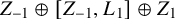
Then we can find two hyperbolic pairs $(x,y)$
and
$(x,y)$
and $(p,q)$
of extremal elements, with corresponding
$(p,q)$
of extremal elements, with corresponding $5$
-gradings
$5$
-gradings
 $$ \begin{align*} L &= L_{-2}\oplus L_{-1}\oplus L_0\oplus L_1\oplus L_2, \\ L &= L^{\prime}_{-2}\oplus L^{\prime}_{-1}\oplus L^{\prime}_0\oplus L^{\prime}_1\oplus L^{\prime}_2, \end{align*} $$
such that the gradings intersect as in Figure 1. Moreover, the structure of the Lie algebra induces various maps between the different components of this $5 \times 5$
-grading, resulting in a ‘twin cubic norm structure’ on the pair
$5 \times 5$
-grading, resulting in a ‘twin cubic norm structure’ on the pair
 $$\begin{align*}J = L_{-1} \cap L^{\prime}_{-1}, \quad J' = L_{-1} \cap L^{\prime}_0. \end{align*}$$
If the norm of this structure is not identically zero, then this results in a genuine cubic norm structure.
Theorem C. Let L be a simple Lie algebra defined over a field k with $|k| \geq 3$
. Assume that L is generated by its pure extremal elements and that
$|k| \geq 3$
. Assume that L is generated by its pure extremal elements and that
-
(i) there exists a Galois extension $k'/k$
of degree at most
$2$
such that the extremal geometry of
$L\otimes k'$
contains lines;
$k'/k$
of degree at most
$2$
such that the extremal geometry of
$L\otimes k'$
contains lines; -
(ii) there exist symplectic pairs of extremal elements.


Then we can find two hyperbolic pairs $(x,y)$
and
$(x,y)$
and $(p,q)$
of extremal elements, with corresponding
$(p,q)$
of extremal elements, with corresponding $5$
-gradings
$5$
-gradings
 $$ \begin{align*} L &= L_{-2}\oplus L_{-1}\oplus L_0\oplus L_1\oplus L_2, \\ L &= L^{\prime}_{-2}\oplus L^{\prime}_{-1}\oplus L^{\prime}_0\oplus L^{\prime}_1\oplus L^{\prime}_2, \end{align*} $$
such that the gradings intersect as in Figure 2. Moreover, the structure of the Lie algebra induces various maps between the different components of this $5 \times 5$
-grading, resulting in a quadrangular algebra on the pair
$5 \times 5$
-grading, resulting in a quadrangular algebra on the pair
 $$\begin{align*}V = L_{-1} \cap L^{\prime}_{-1}, \quad X = L_{-1} \cap L^{\prime}_0. \end{align*}$$
Theorem B is shown in Section 4 culminating in Theorem 4.23, and Theorem C is shown in Section 5 culminating in Theorem 5.56. For both results, we rely in a crucial way on Theorem A. For Theorem B, we use this result to define the norm N and the adjoint $\sharp $
of the cubic norm structure in Definition 4.12, relying on Proposition 4.11. For Theorem C, we use it to define the quadratic form Q on V in Definition 5.10 (relying on Lemma 5.9) and to define the map
$\sharp $
of the cubic norm structure in Definition 4.12, relying on Proposition 4.11. For Theorem C, we use it to define the quadratic form Q on V in Definition 5.10 (relying on Lemma 5.9) and to define the map $\theta \colon X \times V \to V$
in Definition 5.29. Not surprisingly, the corresponding Theorem 3.13 is used in many places of our proof.
$\theta \colon X \times V \to V$
in Definition 5.29. Not surprisingly, the corresponding Theorem 3.13 is used in many places of our proof.
1 Preliminaries
Throughout, k is an arbitrary commutative field of arbitrary characteristic. All algebras occurring in this paper are assumed to be k-algebras. This preliminary section consists of three parts. Section 1.1 deals with Lie algebras and introduces the basic theory of extremal elements and the extremal geometry. Most of this material is taken from [Reference Cohen and IvanyosCI06]. We then introduce cubic norm structures in Section 1.2 and quadrangular algebras in Section 1.3.
1.1 Lie algebras
Definition 1.1. A $\mathbb {Z}$
-grading of a Lie algebra L is a vector space decomposition
$\mathbb {Z}$
-grading of a Lie algebra L is a vector space decomposition $L=\bigoplus _{i\in \mathbb {Z}} L_i$
such that
$L=\bigoplus _{i\in \mathbb {Z}} L_i$
such that $[L_i,L_j]\leq L_{i+j}$
for all
$[L_i,L_j]\leq L_{i+j}$
for all $i,j\in \mathbb {Z}$
. If n is a natural number such that
$i,j\in \mathbb {Z}$
. If n is a natural number such that $L_i=0$
for all
$L_i=0$
for all $i\in \mathbb {Z}$
such that
$i\in \mathbb {Z}$
such that $|i|>n$
while
$|i|>n$
while $L_{-n}\oplus L_n\neq 0$
, then we call this grading a
$L_{-n}\oplus L_n\neq 0$
, then we call this grading a $(2n+1)$
-grading. We call
$(2n+1)$
-grading. We call $L_{-n}$
and
$L_{-n}$
and $L_n$
the ends of this grading. The i-component of
$L_n$
the ends of this grading. The i-component of $x\in L$
is the image of the projection of x onto
$x\in L$
is the image of the projection of x onto $L_i$
. We also set
$L_i$
. We also set $L_{\leq i}=\bigoplus _{j\leq i} L_j$
and
$L_{\leq i}=\bigoplus _{j\leq i} L_j$
and $L_{\geq i}=\bigoplus _{j\geq i} L_j$
.
$L_{\geq i}=\bigoplus _{j\geq i} L_j$
.
Definition 1.2 [Reference Cohen and IvanyosCI06, Definition 14].
Let L be a Lie algebra over k.
-
(i) A nonzero element
$x\in L$
is called extremal if there is a map
$g_x \colon L \to k$
, called the extremal form on x, such that for all
$y,z \in L$
, we have (1)
$$ \begin{align} \big[x,[x,y]\big] &= 2g_x(y)x,\qquad\qquad\qquad\qquad\qquad \end{align} $$
(2)
$$ \begin{align} \big[[x,y],[x,z]\big] &= g_x\big([y,z]\big)x+g_x(z)[x,y]-g_x(y)[x,z], \end{align} $$
(3)
$$ \begin{align} \big[x,[y,[x,z]]\big] &= g_x\big([y,z]\big)x-g_x(z)[x,y]-g_x(y)[x,z]. \end{align} $$
The last two identities are called the Premet identities. If the characteristic of k is not
$2$
, then the Premet identities (2) and (3) follow from (1); see [Reference Cohen and IvanyosCI06, Definition 14]. Moreover, using the Jacobi identity, (2) and (3) are equivalent if (1) holds.Note that the extremal form
$g_x$
might not be unique if
$\operatorname {\mathrm {char}}(k) = 2$
. -
(ii) We call
$x\in L$
a sandwich or an absolute zero divisor if
$[x,[x,y]]=0$
and
$[x,[y,[x,z]]]=0$
for all
$y,z\in L$
. An extremal element is called pure if it is not a sandwich. -
(iii) The Lie algebra L is nondegenerate if it has no nontrivial sandwiches.
-
(iv) We denote the set of extremal elements of a Lie algebra L by
$E(L)$
or, if L is clear from the context, by E. Accordingly, we denote the set
$\{ k x \mid x\in E(L)\}$
of extremal points in the projective space on L by
$\mathcal {E}(L)$
or
$\mathcal {E}$
.


Remark 1.3.
-
(i) If
$x \in L$
is a sandwich, then the extremal form
$g_x$
can be chosen to be identically zero; we adopt the convention from [Reference Cohen and IvanyosCI06] that
$g_x$
is identically zero whenever x is a sandwich in L. -
(ii) By [Reference Cohen and IvanyosCI06, Lemma 16], the existence of two distinct functions
$g_x$
and
$g^{\prime }_x$
satisfying the identities (1) to (3) implies that
$\operatorname {\mathrm {char}}(k)=2$
and that x is a sandwich. Combined with our convention in (i), this means that
$g_x$
is always uniquely determined.


Definition 1.4. Let L be a Lie algebra. An inner ideal of L is a subspace I of L satisfying $[I,[I,L]]\leq I$
.
$[I,[I,L]]\leq I$
.
If $\operatorname {\mathrm {char}}(k) \neq 2$
, then the
$\operatorname {\mathrm {char}}(k) \neq 2$
, then the $1$
-dimensional inner ideals of L are precisely the subspaces spanned by an extremal element. We will need inner ideals of dimension
$1$
-dimensional inner ideals of L are precisely the subspaces spanned by an extremal element. We will need inner ideals of dimension $>1$
only once, namely in the proof of Theorem 3.8.
$>1$
only once, namely in the proof of Theorem 3.8.
Recall that if D is a linear map from a Lie algebra L to itself such that $D^n=0$
for some
$D^n=0$
for some $n\in \mathbb N$
and
$n\in \mathbb N$
and $(n-1)!\in k^\times $
, then
$(n-1)!\in k^\times $
, then $\exp (D)=\sum _{i=0}^{n-1}\frac {1}{i!}D^i$
. A crucial aspect of extremal elements is that they allow for exponential maps in any characteristic.
$\exp (D)=\sum _{i=0}^{n-1}\frac {1}{i!}D^i$
. A crucial aspect of extremal elements is that they allow for exponential maps in any characteristic.
Definition 1.5 [Reference Cohen and IvanyosCI06, p. 444].
Let $x \in E$
be an extremal element, with extremal form
$x \in E$
be an extremal element, with extremal form $g_x$
. Then we define
$g_x$
. Then we define
 $$\begin{align*}\exp(x) \colon L \to L \colon y \mapsto y + [x,y] + g_x(y)x. \end{align*}$$
We also write $\operatorname {\mathrm {Exp}}(x) := \{ \exp (\lambda x) \mid \lambda \in k \}$
.
$\operatorname {\mathrm {Exp}}(x) := \{ \exp (\lambda x) \mid \lambda \in k \}$
.
Lemma 1.6 [Reference Cohen and IvanyosCI06, Lemma 15].
For each $x \in E$
, we have
$x \in E$
, we have $\exp (x) \in \operatorname {\mathrm {Aut}}(L)$
. Moreover,
$\exp (x) \in \operatorname {\mathrm {Aut}}(L)$
. Moreover, $\exp (\lambda x) \exp (\mu x) = \exp ((\lambda + \mu )x)$
for all
$\exp (\lambda x) \exp (\mu x) = \exp ((\lambda + \mu )x)$
for all $\lambda ,\mu \in k$
, so
$\lambda ,\mu \in k$
, so $\operatorname {\mathrm {Exp}}(x)$
is a subgroup of
$\operatorname {\mathrm {Exp}}(x)$
is a subgroup of $\operatorname {\mathrm {Aut}}(L)$
.
$\operatorname {\mathrm {Aut}}(L)$
.
Notice that for an extremal element $x \in E$
, we always have
$x \in E$
, we always have $\operatorname {\mathrm {ad}}_x^3 = 0$
. In particular, if
$\operatorname {\mathrm {ad}}_x^3 = 0$
. In particular, if $\operatorname {\mathrm {char}}(k) \neq 2$
, then
$\operatorname {\mathrm {char}}(k) \neq 2$
, then $g_x(y) x = \tfrac {1}{2} [x, [x, y]]$
, and we recover the usual exponential map
$g_x(y) x = \tfrac {1}{2} [x, [x, y]]$
, and we recover the usual exponential map $\exp (x) = \exp (\operatorname {\mathrm {ad}}_x)$
.
$\exp (x) = \exp (\operatorname {\mathrm {ad}}_x)$
.
In this paper, we will always assume that our Lie algebra L is generated by its extremal elements. This has some powerful consequences.
Proposition 1.7 [Reference Cohen and IvanyosCI06, Proposition 20].
Suppose that L is generated by E. Then
-
(i) L is linearly spanned by E.
-
(ii) There is a unique bilinear form
$g \colon L \times L \to k$
such that
$g_x(y) = g(x,y)$
for all
$x \in E$
and all
$y \in L$
. The form g is symmetric. -
(iii) The form g associates with the Lie bracket (i.e.,
$g([x,y],z) = g(x,[y,z])$
for all
$x,y,z \in L$
).


Proposition 1.8 [Reference Cohen and IvanyosCI06, Lemmas 21, 24, 25 and 27].
Suppose that L is generated by E. Let $x,y \in E$
be pure extremal elements. Then exactly one of the following holds:
$x,y \in E$
be pure extremal elements. Then exactly one of the following holds:
-
(a)
$kx = ky$
; -
(b)
$kx \neq ky$
,
$[x,y] = 0$
, and
$\lambda x + \mu y \in E \cup \{ 0 \}$
for all
$\lambda ,\mu \in k$
(we write
$x \sim y$
); -
(c)
$kx \neq ky$
,
$[x,y] = 0$
, and
$\lambda x + \mu y \in E \cup \{ 0 \}$
if and only if
$\lambda =0$
or
$\mu =0$
; -
(d)
$[x,y] \neq 0$
and
$g(x,y)=0$
, in which case
$[x,y] \in E$
and
$x \sim [x,y] \sim y$
; -
(e)
$[x,y] \neq 0$
and
$g(x,y) \neq 0$
, in which case x and y generate an
$\mathfrak {sl}_2(k)$
-subalgebra.


Moreover, we have $g(x,y) = 0$
in all four cases (a)–(d).
$g(x,y) = 0$
in all four cases (a)–(d).
This gives rise to the following definitions.
Definition 1.9.
-
(i) Let
$\langle x \rangle , \langle y \rangle \in {\mathcal {E}}(L)$
be two distinct pure extremal points. Then depending on whether the corresponding elements
$x,y$
are in case (b), (c), (d) or (e) of Proposition 1.8, we call the pair
$\langle x \rangle , \langle y \rangle $
collinear, symplectic, special or hyperbolic, respectively. Following the notation from [Reference Cohen and IvanyosCI06], we denote the five possible relations between points of
${\mathcal {E}}$
by
${\mathcal {E}}_{-2}$
(equal),
${\mathcal {E}}_{-1}$
(collinear),
${\mathcal {E}}_0$
(symplectic),
${\mathcal {E}}_1$
(special),
${\mathcal {E}}_2$
(hyperbolic), respectively. We also use
$E_{-2},E_{-1},E_0,E_1,E_2$
for the corresponding relations between elements of E. Moreover, we write
$E_i(x)$
for the set of elements of E in relation
$E_i$
with x, and similarly for
${\mathcal {E}}_i(\langle x \rangle )$
.We refer the reader to Proposition 2.5 for the motivation for this notation.
-
(ii) The extremal geometry associated with L is the point-line geometry with point set
${\mathcal {E}}(L)$
and line set
$$\begin{align*}\mathcal{F}(L) := \{ \langle x,y \rangle \mid \langle x \rangle \text{ and } \langle y \rangle \text{ are collinear} \}. \end{align*}$$
It is a partial linear space (i.e., any two distinct points lie on at most one line).


A crucial ingredient for us will be the fact that each hyperbolic pair of extremal elements gives rise to a $5$
-grading of the Lie algebra; see Proposition 2.4 below.
$5$
-grading of the Lie algebra; see Proposition 2.4 below.
We finish this section with a subtle but important fact about exponential maps arising from a $5$
-grading.
$5$
-grading.
Definition 1.10. Assume that $\operatorname {\mathrm {char}}(k) \neq 2,3$
and let L be a 5-graded finite-dimensional Lie algebra over k. We say that L is algebraic if for any
$\operatorname {\mathrm {char}}(k) \neq 2,3$
and let L be a 5-graded finite-dimensional Lie algebra over k. We say that L is algebraic if for any $(x,s) \in L_{\sigma 1} \oplus L_{\sigma 2}$
(with
$(x,s) \in L_{\sigma 1} \oplus L_{\sigma 2}$
(with $\sigma \in \{ +,- \}$
), the linear endomorphism
$\sigma \in \{ +,- \}$
), the linear endomorphism
 $$\begin{align*}\exp(\operatorname{\mathrm{ad}}(x+s)) = \sum_{i=0}^{4} \frac{1}{i!} \operatorname{\mathrm{ad}}(x+s)^i\end{align*}$$
of L is a Lie algebra automorphism.
It is not difficult to see that when $\operatorname {\mathrm {char}}(k) \neq 2,3,5$
, then any
$\operatorname {\mathrm {char}}(k) \neq 2,3,5$
, then any $5$
-graded Lie algebra is algebraic; see [Reference Boelaert, De Medts and StavrovaBDMS19, Lemma 3.1.7]. If
$5$
-graded Lie algebra is algebraic; see [Reference Boelaert, De Medts and StavrovaBDMS19, Lemma 3.1.7]. If $\operatorname {\mathrm {char}}(k) = 5$
, this is much more delicate; see [Reference Boelaert, De Medts and StavrovaBDMS19, §4.2] and [Reference StavrovaSta22, Theorem 2.10].
$\operatorname {\mathrm {char}}(k) = 5$
, this is much more delicate; see [Reference Boelaert, De Medts and StavrovaBDMS19, §4.2] and [Reference StavrovaSta22, Theorem 2.10].
One of our key tools will precisely be an extension of the existence of such automorphisms to the case where $\operatorname {\mathrm {char}}(k)$
is arbitrary, including characteristic
$\operatorname {\mathrm {char}}(k)$
is arbitrary, including characteristic $2$
and
$2$
and $3$
; see Definitions 3.12 and 3.13 and Theorems 3.15 and 3.16 below.
$3$
; see Definitions 3.12 and 3.13 and Theorems 3.15 and 3.16 below.
1.2 Cubic norm structures
Cubic norm structures have been introduced by Kevin McCrimmon in [Reference McCrimmonMcC69]. We follow the approach from [Reference Tits and WeissTW02, Chapter 15], which is equivalent but is more practical for our purposes.
Definition 1.11. A cubic norm structure is a tuple
 $$\begin{align*}(J,k,N,\sharp,T,\times,1),\end{align*}$$
where k is a field, J is a vector space over k, $N \colon J\to k$
is a map called the norm,
$N \colon J\to k$
is a map called the norm, $\sharp \colon J\to J$
is a map called the adjoint,
$\sharp \colon J\to J$
is a map called the adjoint, $T \colon J\times J\to k$
is a symmetric bilinear form called the trace,
$T \colon J\times J\to k$
is a symmetric bilinear form called the trace, $\times \colon J\times J\to J$
is a symmetric bilinear map called the Freudenthal cross product, and
$\times \colon J\times J\to J$
is a symmetric bilinear map called the Freudenthal cross product, and $1$
is a nonzero element of J called the identity such that for all
$1$
is a nonzero element of J called the identity such that for all $\lambda \in k$
, and all
$\lambda \in k$
, and all $a,b,c\in J$
, we have
$a,b,c\in J$
, we have
-
(i)
$(\lambda a)^\sharp =\lambda ^2a^\sharp $
; -
(ii)
$N(\lambda a)=\lambda ^3 N(a)$
; -
(iii)
$T(a,b\times c)=T(a\times b,c)$
; -
(iv)
$(a+b)^\sharp =a^\sharp +a\times b+b^\sharp $
; -
(v)
$N(a+b)=N(a)+T(a^\sharp ,b)+T(a,b^\sharp )+N(b)$
; -
(vi)
$T(a,a^\sharp )=3N(a)$
; -
(vii)
$(a^\sharp )^\sharp =N(a)a$
; -
(viii)
$a^\sharp \times (a\times b)=N(a)b+T(a^\sharp ,b)a$
; -
(ix)
$a^\sharp \times b^\sharp +(a\times b)^\sharp =T(a^\sharp ,b)b+T(a,b^\sharp )a$
; -
(x)
$1^\sharp =1$
; -
(xi)
$a=T(a,1)1-1\times a$
.


We call this cubic norm structure nondegenerate if $\{a\in J\mid N(a)=0=T(a,J)=T(a^\sharp ,J)\} = 0$
.
$\{a\in J\mid N(a)=0=T(a,J)=T(a^\sharp ,J)\} = 0$
.
Definition 1.12. We call $a\in J$
invertible if
$a\in J$
invertible if $N(a)\neq 0$
. We denote the set of all invertible elements of J by
$N(a)\neq 0$
. We denote the set of all invertible elements of J by $J^\times $
. If all nonzero elements of J are invertible, we call J anisotropic; otherwise, we call it isotropic.
$J^\times $
. If all nonzero elements of J are invertible, we call J anisotropic; otherwise, we call it isotropic.
Lemma 1.13 [Reference Tits and WeissTW02, (15.18)].
In Definition 1.11, condition (iii) is a consequence of (iv) and (v). If $|k|>3$
, then conditions (vi), (viii) and (ix) are a consequence of (i), (ii), (iv), (v) and (vii).
$|k|>3$
, then conditions (vi), (viii) and (ix) are a consequence of (i), (ii), (iv), (v) and (vii).
Remark 1.14. Every cubic norm structure can be made into a (quadratic) Jordan algebra, where the U-operator of the Jordan algebra is given by
 $$ \begin{align*} U_x(y)=T(y,x)x-y\times x^\sharp \end{align*} $$
for all $x,y\in J$
.
$x,y\in J$
.
Definition 1.15.
-
(i) Let
$(J,k,N,\sharp ,T,\times , 1)$
and
$(J',k,N',\sharp ',T',\times ', 1')$
be two cubic norm structures. A vector space isomorphism
$\varphi :J\to J'$
is an isomorphism from
$(J,k,N,\sharp ,T,\times , 1)$
to
$(J',k,N',\sharp ',T',\times ', 1')$
if
$\varphi \circ \sharp =\sharp '\circ \varphi $
and
$\varphi (1)=1'$
. -
(ii) Let
$(J,k,N,\sharp ,T,\times ,1)$
be a cubic norm structure and let
$d\in J^\times $
. We define new maps
$N_d$
,
$\sharp _d$
,
$T_d$
,
$\times _d$
and
$1_d$
by for all
$$ \begin{align*} N_d(a) &:= N(d)^{-1} N(a) , \\ a^{\sharp_d} &:= N(d)^{-1} U_d(a^\sharp) , \\ T_d(a,b) &:= T\big( U_{N(d)^{-1} d^\sharp}(a), b \big) , \\ a \times_d b &:= N(d)^{-1} U_d(a \times b) , \\ 1_d &:= d , \end{align*} $$
$a,b \in J$
. Then
$(J,k,N_d,\sharp _d,T_d,\times _d,1_d)$
is again a cubic norm structure; see [Reference Tits and WeissTW02, (29.36)].
Two cubic norm structures
$(J,k,N,\sharp ,T,\times ,1)$
and
$(J',k,N',\sharp ',T',\times ',1')$
are called isotopic if there exists an isomorphism from
$(J',k,N',\sharp ',T',\times ',1')$
to
$(J,k,N_d,\sharp _d,T_d,\times _d,1_d)$
for a certain
$d\in J^\times $
.


1.3 Quadrangular algebras
Quadrangular algebras have been introduced by Richard Weiss in [Reference WeissWei06] in the anisotropic case, and have been generalized to allow isotropic quadrangular algebras in [Reference Mühlherr and WeissMW19]. Our notation follows [Reference Mühlherr and WeissMW19], except that we use different letters for some of our spaces and maps.
Definition 1.16. Let V be a vector space over the field k. A quadratic form Q on V is a map $Q \colon V\to k$
such that
$Q \colon V\to k$
such that
-
○
$Q(\lambda v)=\lambda ^2Q(v)$
for all
$\lambda \in k$
and
$v\in V$
; -
○ the map
$T \colon V\times V\to k$
defined by for all
$$\begin{align*}T(u,v)=Q(u+v)-Q(u)-Q(v) \end{align*}$$
$u,v \in V$
is bilinear.


We call Q
-
○ anisotropic if
$Q(v)=0$
implies
$v=0$
; -
○ nondegenerate if
$V^\perp := \{ v\in V \mid T(v,V)=0 \} = 0$
; -
○ non-singular if it is either nondegenerate or
$\dim (V^\perp )=1$
and
$Q(V^\perp )\neq 0$
; -
○ regular if
$\{ v \in V \mid Q(v)=0=T(v,V) \} = 0$
.


A base point for Q is an element $e\in V$
such that
$e\in V$
such that $Q(e)=1$
. Using this base point, we can define an involution
$Q(e)=1$
. Using this base point, we can define an involution $\sigma \colon V\to V$
by
$\sigma \colon V\to V$
by
 $$ \begin{align} v^\sigma = T(v,e)e - v, \end{align} $$
for all $v\in V$
.
$v\in V$
.
Definition 1.17 [Reference Mühlherr and WeissMW19, Definition 2.1].
A quadrangular algebra is a tuple
 $$\begin{align*}(k,V,Q,T,e,X,\cdot,h,\theta),\end{align*}$$
where
-
○ k is a field;
-
○ V is a vector space over k;
-
○
$Q \colon V \to k$
is a regular quadratic form, with associated bilinear form T; -
○
$e \in V$
is a base point for Q; -
○ X is a vector space over k;
-
○
$\cdot \colon X\times V \to X \colon (a,v)\mapsto a \cdot v$
is a bilinear map; -
○
$h \colon X\times X\to V$
is a bilinear map; -
○
$\theta \colon X\times V\to V$
is a map;


such that
-
(i)
$a \cdot e=a$
for all
$a\in X$
; -
(ii)
$(a\cdot v)\cdot v^\sigma = Q(v)a$
for all
$a\in X$
and all
$v\in V$
; -
(iii)
$h(a, b \cdot v) = h(b, a \cdot v) + T(h(a,b), e)v$
for all
$a,b \in X$
and all
$v\in V$
; -
(iv)
$T(h(a\cdot v, b), e) = T(h(a,b), v)$
for all
$a,b \in X$
and all
$v\in V$
; -
(v) For each
$a \in X$
, the map
$v \mapsto \theta (a,v)$
is linear; -
(vi)
$\theta (\lambda a, v) = \lambda ^2 \theta (a, v)$
for all
$a \in X$
,
$v \in V$
and
$\lambda \in k$
; -
(vii) There exists a function
$\gamma \colon X\times X\to k$
such that for all
$$\begin{align*}\theta(a+b, v) = \theta(a,v) + \theta(b,v) + h(a, b\cdot v) - \gamma(a,b)v \end{align*}$$
$a,b\in X$
and all
$v\in V$
;
-
(viii) There exists a function
$\phi \colon X\times V \to k$
such that for all
$$ \begin{align*} \theta(a\cdot v, w) = \theta(a, w^\sigma)^\sigma Q(v) - T(w, v^\sigma) \theta(a,v)^\sigma + T(\theta(a,v), w^\sigma) v^\sigma + \phi(a,v)w \end{align*} $$
$a\in X$
and all
$v,w \in V$
;
-
(ix)
$a \cdot \theta (a,v) = (a \cdot \theta (a,e)) \cdot v$
for all
$a\in X$
and all
$v\in V$
.


Notation 1.18. We set $\pi (a)=\theta (a,e)$
for all
$\pi (a)=\theta (a,e)$
for all $a\in X$
.
$a\in X$
.
Definition 1.19 [Reference Mühlherr and WeissMW19, Definition 2.3].
We call a quadrangular algebra anisotropic if Q is anisotropic and $\pi (a)$
is a multiple of e if and only if
$\pi (a)$
is a multiple of e if and only if $a=0$
.
$a=0$
.
Remark 1.20. The existence of $e \in V$
implies
$e \in V$
implies $V\neq 0$
. However, contrary to the common convention, we allow
$V\neq 0$
. However, contrary to the common convention, we allow $X=0$
. In other words, we view quadratic spaces as special (degenerate) examples of quadrangular algebras.
$X=0$
. In other words, we view quadratic spaces as special (degenerate) examples of quadrangular algebras.
2 Gradings from extremal elements
In this section, we describe the $5$
-grading associated with any pair of hyperbolic extremal elements, and we collect several properties about this grading that we will need later. We emphasize again that we do not make any assumptions on the field k, so in particular, we allow
$5$
-grading associated with any pair of hyperbolic extremal elements, and we collect several properties about this grading that we will need later. We emphasize again that we do not make any assumptions on the field k, so in particular, we allow $\operatorname {\mathrm {char}}(k) = 2$
or
$\operatorname {\mathrm {char}}(k) = 2$
or $3$
.
$3$
.
Notation 2.1. We will assume from now on that L is a Lie algebra over k generated by its pure extremal elements. As in Definition 1.2, we will write E for the set of extremal elements of L and ${\mathcal {E}}$
for the set of extremal points of L. We let g be the symmetric bilinear form from Proposition 1.7. If V is any subspace of L, we write
${\mathcal {E}}$
for the set of extremal points of L. We let g be the symmetric bilinear form from Proposition 1.7. If V is any subspace of L, we write
 $$\begin{align*}V^\perp := \{ u \in L \mid g(u,v) = 0 \text{ for all } v \in V \}. \end{align*}$$
Remark 2.2. If, in addition, L is simple, then our assumptions imply that L does not contain sandwich elements. Indeed, the sandwich elements are contained in the radical of the form g, which is an ideal of L. Since L is generated by its pure extremal elements, the form g cannot be identically zero, so the radical of g must be trivial.
In this section, we do not assume that L is simple (except in Lemma 2.11 and Propositions 2.13 and 2.16), but we will make this important assumption in the next sections.
Definition 2.3. We define the normalizer of x as
 $$\begin{align*}N_L(x) := \big\{ l \in L \mid [x,l] \in \langle x \rangle \big \}. \end{align*}$$
Proposition 2.4 [Reference Cohen and IvanyosCI06, Proposition 22 and Corollary 23].
Let $x, y\in E$
such that
$x, y\in E$
such that $g(x,y)=1$
. Then
$g(x,y)=1$
. Then
-
(i) L has a
$\mathbb {Z}$
-grading with
$$\begin{align*}L=L_{-2}\oplus L_{-1}\oplus L_0\oplus L_1\oplus L_2,\end{align*}$$
$L_{-2}=\langle x\rangle $
,
$L_{-1}=[x,U]$
,
$L_0=N_{L}(x)\cap N_{L}(y)$
,
$L_1=[y,U]$
and
$L_2=\langle y\rangle $
, where
$$\begin{align*}U = \big\langle x, y, [x,y] \big\rangle^\perp. \end{align*}$$
-
(ii) Each
$L_i$
is contained in the i-eigenspace of
$\operatorname {\mathrm {ad}}_{[x,y]}$
. -
(iii)
$\operatorname {\mathrm {ad}}_x$
defines a linear isomorphism from
$L_1$
to
$L_{-1}$
with inverse
$-\operatorname {\mathrm {ad}}_y$
. -
(iv) The filtration
$L_{-2} \leq L_{\leq -1} \leq L_{\leq 0} \leq L_{\leq 1} \leq L$
only depends on x and not on y. More precisely, we have
$$ \begin{align*} L_{\leq 1} &= x^\perp, \\ L_{\leq 0} &= N_L(x), \\ L_{\leq -1} &= kx + [x, x^\perp], \\ L_{-2} &= kx. \end{align*} $$
-
(v) In particular,
$g_x(L_{\leq 1})=0$
and
$g_y(L_{\geq -1})=0$
.


These gradings are closely related to the five different relations $E_i$
that we have introduced in Definition 1.9:
$E_i$
that we have introduced in Definition 1.9:
Proposition 2.5. Let x, y and $L_i$
be as in Proposition 2.4. For each
$L_i$
be as in Proposition 2.4. For each $i\in [-2,2]$
, we have
$i\in [-2,2]$
, we have
 $$\begin{align*}E_i(x)=(E\cap L_{\leq i}) \setminus L_{\leq i-1}. \end{align*}$$
Proof. This is shown in the proof of [Reference Cohen and IvanyosCI06, Theorem 28].
Corollary 2.6. Let x, y and $L_i$
be as in Proposition 2.4. Then
$L_i$
be as in Proposition 2.4. Then
 $$\begin{align*}E_{-1}(x) = \{ \lambda x + e \mid \lambda \in k, e \in E \cap L_{-1} \}. \end{align*}$$
Proof. By Proposition 2.5, $E_{-1}(x) = E \cap (kx + L_{-1}) \setminus kx$
. Now observe that an element
$E_{-1}(x) = E \cap (kx + L_{-1}) \setminus kx$
. Now observe that an element $\lambda x + e$
(with
$\lambda x + e$
(with $e \in L_{-1}$
) is extremal if and only if e is extremal, because if one of them is extremal, it is collinear with x, and hence, all points on the line through x are extremal points.
$e \in L_{-1}$
) is extremal if and only if e is extremal, because if one of them is extremal, it is collinear with x, and hence, all points on the line through x are extremal points.
Lemma 2.7. Let x, y and $L_i$
be as in Proposition 2.4. Let
$L_i$
be as in Proposition 2.4. Let $a \in L_1$
and
$a \in L_1$
and $b \in L_{-1}$
. Then
$b \in L_{-1}$
. Then $[a, [y,b]] = g(a,b)y$
.
$[a, [y,b]] = g(a,b)y$
.
Proof. By Proposition 2.4(iii), we can write $a = [y,c]$
for some
$a = [y,c]$
for some $c \in L_{-1}$
. By the Premet identity (2) and Proposition 2.4(v), we then get
$c \in L_{-1}$
. By the Premet identity (2) and Proposition 2.4(v), we then get
 $$ \begin{align*} [a, [y,b]] &= [[y,c], [y,b]] \\ &= g_y([c,b])y + g_y(b) [y,c] - g_y(c) [y,b] \\ &= g(y, [c,b])y = g([y,c], b)y = g(a,b)y. \end{align*} $$
The following lemma describes an automorphism that reverses the grading.
Lemma 2.8. Let x, y and $L_i$
be as in Proposition 2.4. Consider the automorphism
$L_i$
be as in Proposition 2.4. Consider the automorphism $\varphi =\exp (y)\exp (x)\exp (y)$
. Then
$\varphi =\exp (y)\exp (x)\exp (y)$
. Then
 $$ \begin{align*} \varphi(x) &= y , \\ \varphi(l_{-1}) &= [y, l_{-1}] , \\ \varphi(l_0) &= l_0 + [x, [y, l_0]] , \\ \varphi(l_1) &= [x, l_1] , \\ \varphi(y) &= x , \end{align*} $$
for all $l_{-1} \in L_{-1}$
,
$l_{-1} \in L_{-1}$
, $l_0 \in L_0$
,
$l_0 \in L_0$
, $l_1 \in L_1$
.
$l_1 \in L_1$
.
Proof. Since $g_x(y)=g_y(x)=1$
, we get
$g_x(y)=g_y(x)=1$
, we get $\exp (x)(y) = y + [x,y] + x$
and
$\exp (x)(y) = y + [x,y] + x$
and $\exp (y)(x) = x - [x,y] + y$
. Since
$\exp (y)(x) = x - [x,y] + y$
. Since $g_x([x,y]) = 0$
and
$g_x([x,y]) = 0$
and $g_y([x,y]) = 0$
, it now follows that
$g_y([x,y]) = 0$
, it now follows that $\varphi (x)=y$
and
$\varphi (x)=y$
and $\varphi (y)=x$
.
$\varphi (y)=x$
.
Next, let $l_1\in L_1$
. Then
$l_1\in L_1$
. Then $\exp (y)(l_1) = l_1$
and
$\exp (y)(l_1) = l_1$
and $\exp (x)(l_1) = l_1 + [x, l_1]$
because
$\exp (x)(l_1) = l_1 + [x, l_1]$
because $g_x(L_1) = 0$
(by Proposition 2.4(v)). By the same Proposition 2.4(v), we also have
$g_x(L_1) = 0$
(by Proposition 2.4(v)). By the same Proposition 2.4(v), we also have $g_y(L_{-1}) = 0$
, and hence,
$g_y(L_{-1}) = 0$
, and hence,
 $$\begin{align*}\varphi(l_1)=\exp(y)([x,l_1]+l_1)=[x,l_1]+ \big( l_1+[y,[x,l_1]] \big) = [x,l_1] , \end{align*}$$
by Proposition 2.4(iii). Similarly, $\varphi (l_{-1})=[y,l_{-1}]$
for all
$\varphi (l_{-1})=[y,l_{-1}]$
for all $l_{-1}\in L_{-1}$
.
$l_{-1}\in L_{-1}$
.
Finally, let $l_0\in L_0$
. Let
$l_0\in L_0$
. Let $\lambda ,\mu \in k$
be such that
$\lambda ,\mu \in k$
be such that $[x,l_0]=\lambda x$
and
$[x,l_0]=\lambda x$
and $[y,l_0]=\mu y$
. Then by the fact that g associates with the Lie bracket, we have
$[y,l_0]=\mu y$
. Then by the fact that g associates with the Lie bracket, we have
 $$\begin{align*}\mu = g_x(\mu y) = g_x([y,l_0]) = -g_y([x,l_0]) = -g_y(\lambda x) = -\lambda. \end{align*}$$
Hence,
 $$ \begin{align*} \varphi(l_0) &= \exp(y)\exp(x)(l_0 - \lambda y) \\ &= \exp(y) (l_0 + \lambda x) - \lambda \varphi(y) \\ &= (l_0 - \lambda y) + \lambda (x - [x,y] + y) - \lambda x \\ &= l_0 - \lambda [x,y] = l_0 + [x,[y,l_0]].\\[-34pt] \end{align*} $$
Remark 2.9. Because of Lemma 2.8, many results involving the $5$
-grading can be ‘swapped around’. We will often do this without explicitly mentioning.
$5$
-grading can be ‘swapped around’. We will often do this without explicitly mentioning.
The automorphism group $\operatorname {\mathrm {Aut}}(L)$
contains a torus preserving the grading. (This easy fact is, of course, true for any
$\operatorname {\mathrm {Aut}}(L)$
contains a torus preserving the grading. (This easy fact is, of course, true for any $\mathbb {Z}$
-graded algebra.)
$\mathbb {Z}$
-graded algebra.)
Lemma 2.10. Let x, y and $L_i$
be as in Proposition 2.4. Let
$L_i$
be as in Proposition 2.4. Let $\lambda \in k^\times $
be arbitrary. Consider the map
$\lambda \in k^\times $
be arbitrary. Consider the map $\varphi _\lambda \colon L\to L$
defined by
$\varphi _\lambda \colon L\to L$
defined by $\varphi _\lambda (l_i)=\lambda ^il_i$
for all
$\varphi _\lambda (l_i)=\lambda ^il_i$
for all $l_i\in L_i$
, with
$l_i\in L_i$
, with $i\in [-2, 2]$
. Then
$i\in [-2, 2]$
. Then $\varphi _\lambda \in \operatorname {\mathrm {Aut}}(L)$
.
$\varphi _\lambda \in \operatorname {\mathrm {Aut}}(L)$
.
Proof. Clearly, $\varphi _\lambda $
is bijective. Consider
$\varphi _\lambda $
is bijective. Consider $l_i\in L_i$
and
$l_i\in L_i$
and $l_j\in L_j$
arbitrary, with
$l_j\in L_j$
arbitrary, with $i,j\in [-2, 2]$
. Then
$i,j\in [-2, 2]$
. Then
 $$\begin{align*}\varphi_\lambda ([l_i,l_j])=\lambda^{i+j}[l_i,l_j]=[\lambda^il_i,\lambda^jl_j]=[\varphi_\lambda(l_i),\varphi_\lambda(l_j)].\\[-37pt] \end{align*}$$
The following lemma will ensure the nondegeneracy of certain maps later on.
Lemma 2.11. Assume that L is simple, and let x, y and $L_i$
be as in Proposition 2.4. Let
$L_i$
be as in Proposition 2.4. Let $Z_i = \{ z \in L_i \mid [z, L_i] = 0 \}$
for
$Z_i = \{ z \in L_i \mid [z, L_i] = 0 \}$
for $i = -1$
and
$i = -1$
and $i = 1$
. Then
$i = 1$
. Then $Z_{-1} = Z_1 = 0$
.
$Z_{-1} = Z_1 = 0$
.
Proof. Let $z\in Z_{-1}$
and
$z\in Z_{-1}$
and $a\in L_{-1}$
. Then
$a\in L_{-1}$
. Then $[a,z] = 0$
by definition of
$[a,z] = 0$
by definition of $Z_{-1}$
, and
$Z_{-1}$
, and $g_y(z) = g_y(a) = 0$
by Proposition 2.4(v). By the Premet identities, we then have
$g_y(z) = g_y(a) = 0$
by Proposition 2.4(v). By the Premet identities, we then have
 $$\begin{align*}[[y,a],[y,z]]=g_y([a,z])+g_y(z)[y,a]-g_y(a)[y,z]=0. \end{align*}$$
Since $[y, L_{-1}] = L_1$
by Proposition 2.4(iii), this shows that
$[y, L_{-1}] = L_1$
by Proposition 2.4(iii), this shows that $[y,Z_{-1}]\leq Z_1$
. Similarly,
$[y,Z_{-1}]\leq Z_1$
. Similarly, $[x, Z_1] \leq Z_{-1}$
, but then
$[x, Z_1] \leq Z_{-1}$
, but then $Z_{-1} = [x, [y, Z_{-1}]] \leq [x, Z_1] \leq Z_{-1}$
, so in fact,
$Z_{-1} = [x, [y, Z_{-1}]] \leq [x, Z_1] \leq Z_{-1}$
, so in fact,
 $$\begin{align*}[y, Z_{-1}] = Z_1 \quad \text{and} \quad [x, Z_1] = Z_{-1}. \end{align*}$$
Observe now that by the Jacobi identity, $[[L_0,Z_{-1}],L_{-1}] \leq [L_0,[Z_{-1},L_{-1}]]+[Z_{-1},[L_0,L_{-1}]]=0$
, and thus,
$[[L_0,Z_{-1}],L_{-1}] \leq [L_0,[Z_{-1},L_{-1}]]+[Z_{-1},[L_0,L_{-1}]]=0$
, and thus, $[L_0,Z_{-1}]\leq Z_{-1}$
; similarly, we have
$[L_0,Z_{-1}]\leq Z_{-1}$
; similarly, we have $[L_0,Z_1]\leq Z_1$
. Moreover,
$[L_0,Z_1]\leq Z_1$
. Moreover,
 $$\begin{align*}[y,[Z_{-1},L_1]]=[[y,Z_{-1}],L_1]=[Z_1,L_1]=0 , \end{align*}$$
and hence, the map $\varphi $
from Lemma 2.8 fixes
$\varphi $
from Lemma 2.8 fixes $[Z_{-1}, L_1]$
. However,
$[Z_{-1}, L_1]$
. However, $\varphi (Z_{-1}) = [y, Z_{-1}] = Z_1$
and
$\varphi (Z_{-1}) = [y, Z_{-1}] = Z_1$
and $\varphi (L_1) = [x, L_1] = L_{-1}$
, and therefore,
$\varphi (L_1) = [x, L_1] = L_{-1}$
, and therefore, $[Z_{-1},L_1] = [Z_1,L_{-1}]$
. We can now see that
$[Z_{-1},L_1] = [Z_1,L_{-1}]$
. We can now see that
 $$\begin{align*}Z_{-1}\oplus [Z_{-1},L_1]\oplus Z_1 \end{align*}$$
is an ideal of L. Because L is simple, we conclude that $Z_{-1}=0$
and
$Z_{-1}=0$
and $Z_1=0$
.
$Z_1=0$
.
The idea of looking at two different $5$
-gradings obtained from hyperbolic pairs is a key ingredient for our results. The following lemma is a very first (easy) instance of this.
$5$
-gradings obtained from hyperbolic pairs is a key ingredient for our results. The following lemma is a very first (easy) instance of this.
Lemma 2.12. Consider $x,y,a,b\in E$
such that
$x,y,a,b\in E$
such that $g_x(y)=1=g_a(b)$
. Let
$g_x(y)=1=g_a(b)$
. Let
 $$ \begin{align*} L &= L_{-2}\oplus L_{-1}\oplus L_0\oplus L_1\oplus L_2 \quad \text{and} \\ L &= L^{\prime}_{-2}\oplus L^{\prime}_{-1}\oplus L^{\prime}_0\oplus L^{\prime}_1\oplus L^{\prime}_2 \end{align*} $$
be the $5$
-gradings corresponding to the hyperbolic pairs
$5$
-gradings corresponding to the hyperbolic pairs $(x,y)$
and
$(x,y)$
and $(a,b)$
, respectively, as in Proposition 2.4.
$(a,b)$
, respectively, as in Proposition 2.4.
If $\varphi \in \operatorname {\mathrm {Aut}}(L)$
maps
$\varphi \in \operatorname {\mathrm {Aut}}(L)$
maps $L_{-2}$
to
$L_{-2}$
to $L^{\prime }_{-2}$
and
$L^{\prime }_{-2}$
and $L_2$
to
$L_2$
to $L^{\prime }_2$
, then
$L^{\prime }_2$
, then $\varphi (L_i)=L^{\prime }_i$
for all
$\varphi (L_i)=L^{\prime }_i$
for all $i\in [-2,2]$
.
$i\in [-2,2]$
.
Proof. By assumption, there exist $\lambda ,\mu \in k^\times $
such that
$\lambda ,\mu \in k^\times $
such that $\varphi (x)=\lambda a$
and
$\varphi (x)=\lambda a$
and $\varphi (y)=\mu b$
. We have
$\varphi (y)=\mu b$
. We have $L_0=N_L(x)\cap N_L(y)$
and
$L_0=N_L(x)\cap N_L(y)$
and $L^{\prime }_0=N_L(a)\cap N_L(b)$
by Proposition 2.4, so
$L^{\prime }_0=N_L(a)\cap N_L(b)$
by Proposition 2.4, so $L_0$
is mapped to
$L_0$
is mapped to $L^{\prime }_0$
by
$L^{\prime }_0$
by $\varphi $
.
$\varphi $
.
Next, let $U = \langle x, y, [x,y] \rangle ^\perp $
and
$U = \langle x, y, [x,y] \rangle ^\perp $
and $U' = \langle a, b, [a,b] \rangle ^\perp $
. By Remark 1.3 and Proposition 1.7(ii), the form g is uniquely determined by the Lie algebra L, so
$U' = \langle a, b, [a,b] \rangle ^\perp $
. By Remark 1.3 and Proposition 1.7(ii), the form g is uniquely determined by the Lie algebra L, so $\varphi (U) = U'$
. (Recall that ‘
$\varphi (U) = U'$
. (Recall that ‘ $\perp $
’ is with respect to g.) It follows that
$\perp $
’ is with respect to g.) It follows that $\varphi $
maps
$\varphi $
maps $L_{-1} = [x,U]$
to
$L_{-1} = [x,U]$
to $L^{\prime }_{-1} = [a,U']$
and
$L^{\prime }_{-1} = [a,U']$
and $L_1 = [y,U]$
to
$L_1 = [y,U]$
to $L^{\prime }_1 = [b, U']$
.
$L^{\prime }_1 = [b, U']$
.
In Proposition 2.16, we will show that if L is simple and the extremal geometry has lines, we can write x and y as the Lie bracket of two extremal elements in $L_{-1}$
and
$L_{-1}$
and $L_1$
, respectively. We first recall some geometric facts from [Reference Cohen and IvanyosCI06].
$L_1$
, respectively. We first recall some geometric facts from [Reference Cohen and IvanyosCI06].
Proposition 2.13. Assume that L is simple and that the extremal geometry contains lines (i.e., $\mathcal {F}(L) \neq \emptyset $
). Let
$\mathcal {F}(L) \neq \emptyset $
). Let $x,y \in {\mathcal {E}}$
. Then
$x,y \in {\mathcal {E}}$
. Then
-
(i) If
$(x,y) \in E_{-1}$
, then
$E_{-1}(x) \cap E_{1}(y) \neq \emptyset $
. -
(ii) If
$(x,y) \in E_0$
, then
$E_0(x) \cap E_{2}(y) \neq \emptyset $
. -
(iii) If
$(x,y) \in E_1$
, then
$E_{-1}(x) \cap E_{2}(y) \neq \emptyset $
. -
(iv) If
$(x,y) \in E_2$
, then
$E_{-1}(x) \cap E_{1}(y) \neq \emptyset $
, while
$E_{-1}(x) \cap E_{\leq 0}(y) = \emptyset $
.


Proof. By Remark 2.2, L does not contain sandwich elements. By [Reference Cohen and IvanyosCI06, Theorem 28], $({\mathcal {E}}, \mathcal {F})$
is a so-called root filtration space, which is either nondegenerate or has an empty set of lines. By our assumption, the latter case does not occur.
$({\mathcal {E}}, \mathcal {F})$
is a so-called root filtration space, which is either nondegenerate or has an empty set of lines. By our assumption, the latter case does not occur.
In particular, the statements of [Reference Cohen and IvanyosCI06, Lemmas 1 and 4] and [Reference Cohen and IvanyosCI07, Lemma 8] hold. Now claim (i) is [Reference Cohen and IvanyosCI06, Lemma 4(ii)] and claim (ii) is [Reference Cohen and IvanyosCI07, Lemma 8(ii)]. To show claim (iii), let $z := [x,y]$
, so
$z := [x,y]$
, so $(z,x) \in E_{-1}$
. By (i), we can find some
$(z,x) \in E_{-1}$
. By (i), we can find some $u \in E_{-1}(x) \cap E_1(u)$
. We can now invoke [Reference Cohen and IvanyosCI06, Lemma 1(v)] on the pairs
$u \in E_{-1}(x) \cap E_1(u)$
. We can now invoke [Reference Cohen and IvanyosCI06, Lemma 1(v)] on the pairs $(y,x)$
and
$(y,x)$
and $(z,u)$
to conclude that
$(z,u)$
to conclude that $u \in E_{-1}(x) \cap E_2(y)$
.
$u \in E_{-1}(x) \cap E_2(y)$
.
Finally, to show (iv), we first observe that the nondegeneracy of the root filtration space implies that $E_{-1}(x) \neq \emptyset $
(this is condition (H) on [Reference Cohen and IvanyosCI06, p. 439]) and hence, there exists a line
$E_{-1}(x) \neq \emptyset $
(this is condition (H) on [Reference Cohen and IvanyosCI06, p. 439]) and hence, there exists a line $\ell $
through
$\ell $
through $\langle x \rangle $
. We now use the defining properties (D) and (F) of a root filtration space (see [Reference Cohen and IvanyosCI06, p. 435]) to see that
$\langle x \rangle $
. We now use the defining properties (D) and (F) of a root filtration space (see [Reference Cohen and IvanyosCI06, p. 435]) to see that ${\mathcal {E}}_1(y)$
has nonempty intersection with
${\mathcal {E}}_1(y)$
has nonempty intersection with $\ell $
, as required. The final statement
$\ell $
, as required. The final statement $E_{-1}(x) \cap E_{\leq 0}(y) = \emptyset $
is just the defining property (D) itself.
$E_{-1}(x) \cap E_{\leq 0}(y) = \emptyset $
is just the defining property (D) itself.
Lemma 2.14. Let x, y and $L_i$
be as in Proposition 2.4. Then
$L_i$
be as in Proposition 2.4. Then $E_{-1}(x) \cap E_1(y) = E \cap L_{-1}$
.
$E_{-1}(x) \cap E_1(y) = E \cap L_{-1}$
.
Proof. By Proposition 2.5, we have $E_{-1}(x) = (E \cap L_{\leq -1}) \setminus L_{-2}$
. Similarly (e.g., by applying Lemma 2.8; see Remark 2.9), we have
$E_{-1}(x) = (E \cap L_{\leq -1}) \setminus L_{-2}$
. Similarly (e.g., by applying Lemma 2.8; see Remark 2.9), we have $E_1(y) = (E \cap L_{\geq {-1}}) \setminus L_{\geq 0}$
. We conclude that
$E_1(y) = (E \cap L_{\geq {-1}}) \setminus L_{\geq 0}$
. We conclude that $E_{-1}(x) \cap E_1(y) = E \cap L_{-1}$
.
$E_{-1}(x) \cap E_1(y) = E \cap L_{-1}$
.
Lemma 2.15. Let x, y and $L_i$
be as in Proposition 2.4. Consider
$L_i$
be as in Proposition 2.4. Consider $e\in E\cap L_{1}$
. Then
$e\in E\cap L_{1}$
. Then $g_e(x)=0$
for all
$g_e(x)=0$
for all $x\in L_{i}$
with
$x\in L_{i}$
with $i\neq -1$
.
$i\neq -1$
.
Proof. By Proposition 2.4(v), we have $g_e(x)=0$
and
$g_e(x)=0$
and $g_e(y)=0$
. Moreover, for any
$g_e(y)=0$
. Moreover, for any $l\in L_1$
, there exists
$l\in L_1$
, there exists $l'\in L_{-1}$
such that
$l'\in L_{-1}$
such that $l=[y,l']$
by Proposition 2.4. Since g associates with the Lie bracket, we have
$l=[y,l']$
by Proposition 2.4. Since g associates with the Lie bracket, we have
 $$\begin{align*}g_e(l) = g_e([y,l']) = g([e,y],l') = 0. \end{align*}$$
Finally, let $l \in L_0$
. By Proposition 2.4 again, there exist
$l \in L_0$
. By Proposition 2.4 again, there exist $e'\in L_{-1}$
such that
$e'\in L_{-1}$
such that $e=[y,e']$
. Let
$e=[y,e']$
. Let $\lambda \in k$
such that
$\lambda \in k$
such that $[y,l]=\lambda y$
. Then
$[y,l]=\lambda y$
. Then
 $$\begin{align*}g_e(l) = g([y,e'],l)=-g(e',[y,l])=\lambda g_y(e')=0.\\[-37pt] \end{align*}$$
Proposition 2.16. Assume that L is simple and that the extremal geometry of L contains lines. Let $x, y$
and
$x, y$
and $L_i$
be as in Proposition 2.4. Then there exist
$L_i$
be as in Proposition 2.4. Then there exist $c,d\in E\cap L_{-1}$
such that
$c,d\in E\cap L_{-1}$
such that $[c,d]=x$
. Moreover,
$[c,d]=x$
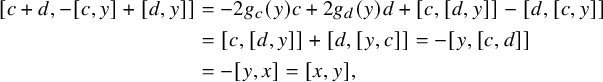
. Moreover,
 $$\begin{align*}[x,y] = [c+d, -[c,y]+[d,y]] \in [I_{-1}, I_1] , \end{align*}$$
where $I_i$
is the subspace of
$I_i$
is the subspace of $L_i$
spanned by
$L_i$
spanned by $E \cap L_i$
, for
$E \cap L_i$
, for $i = \pm 1$
.
$i = \pm 1$
.
Proof. By Proposition 2.13(iv), there exists an $a \in E_{-1}(x) \cap E_{1}(y)$
. By Lemma 2.14,
$a \in E_{-1}(x) \cap E_{1}(y)$
. By Lemma 2.14, $a\in E \cap L_{-1}$
.
$a\in E \cap L_{-1}$
.
Now, by Proposition 2.13(i), we can find some $b \in E_{-1}(x) \cap E_1(a)$
. By Corollary 2.6, we can write
$b \in E_{-1}(x) \cap E_1(a)$
. By Corollary 2.6, we can write $b = \lambda x + d$
with
$b = \lambda x + d$
with $d \in E \cap L_{-1}$
. Moreover,
$d \in E \cap L_{-1}$
. Moreover, $[a, d] = [a, b]$
, and since the pair
$[a, d] = [a, b]$
, and since the pair $(a,b)$
is special and both a and b are collinear with x, we must have
$(a,b)$
is special and both a and b are collinear with x, we must have $[a,b] = \lambda x$
for some
$[a,b] = \lambda x$
for some $\lambda \in k^\times $
. Now write
$\lambda \in k^\times $
. Now write $c = \lambda ^{-1} a$
, and we get
$c = \lambda ^{-1} a$
, and we get $[c, d] = x$
, as required.
$[c, d] = x$
, as required.
Next, observe that $g(c, y) = 0$
and
$g(c, y) = 0$
and $g(d, y) = 0$
because these pairs are special. Using the Jacobi identity, we get
$g(d, y) = 0$
because these pairs are special. Using the Jacobi identity, we get
 $$ \begin{align*} [c+d,-[c,y]+[d,y]]&=-2g_{c}(y)c+2g_{d}(y)d+[c,[d,y]]-[d,[c,y]] \\ &= [c,[d,y]]+[d,[y,c]]=-[y,[c,d]]\\ &=-[y,x]=[x,y], \end{align*} $$
as claimed.
3 l-exponential automorphisms
In this section, we consider a simple Lie algebra over the field $k\neq \mathbb F_2$
which is generated by its pure extremal elements. Such a Lie algebra admits hyperbolic pairs of extremal elements, and by Proposition 2.4, each such pair gives rise to a
$k\neq \mathbb F_2$
which is generated by its pure extremal elements. Such a Lie algebra admits hyperbolic pairs of extremal elements, and by Proposition 2.4, each such pair gives rise to a $5$
-grading
$5$
-grading $L = L_{-2} \oplus L_{-1} \oplus L_0 \oplus L_1 \oplus L_2$
. The main goal of this section is to define automorphisms that behave like exponential automorphisms, with respect to elements of
$L = L_{-2} \oplus L_{-1} \oplus L_0 \oplus L_1 \oplus L_2$
. The main goal of this section is to define automorphisms that behave like exponential automorphisms, with respect to elements of $L_1$
(or
$L_1$
(or $L_{-1}$
). If
$L_{-1}$
). If $l \in L_1$
, then we call the corresponding automorphisms l-exponential. We introduce these in Definition 3.12 and prove their existence and uniqueness (up to a one-parameter choice) in Theorems 3.13 and 3.16.
$l \in L_1$
, then we call the corresponding automorphisms l-exponential. We introduce these in Definition 3.12 and prove their existence and uniqueness (up to a one-parameter choice) in Theorems 3.13 and 3.16.
We first need an auxiliary result; namely, we show in Theorem 3.8 that if the extremal geometry of L contains lines, then $L_1$
is spanned by the extremal elements contained in
$L_1$
is spanned by the extremal elements contained in $L_1$
(and similarly for
$L_1$
(and similarly for $L_{-1}$
). We will need this condition on the existence of lines in Theorem 3.13, but in Theorem 3.16, we will use a Galois descent technique that will allow us to get the same existence and uniqueness results under a much weaker condition – namely, the existence of lines after extending the scalars by a Galois extension.
$L_{-1}$
). We will need this condition on the existence of lines in Theorem 3.13, but in Theorem 3.16, we will use a Galois descent technique that will allow us to get the same existence and uniqueness results under a much weaker condition – namely, the existence of lines after extending the scalars by a Galois extension.
The existence and uniqueness of these automorphisms will play a key role in Sections 4 and 5.
Assumption 3.1. We assume in this section that L is a simple Lie algebra generated by its set E of pure extremal elements. We also assume that $k \neq \mathbb F_2$
. Notice that this implies that L does not contain sandwich elements, and by [Reference Cohen and IvanyosCI06, Theorem 28], the graph
$k \neq \mathbb F_2$
. Notice that this implies that L does not contain sandwich elements, and by [Reference Cohen and IvanyosCI06, Theorem 28], the graph $({\mathcal {E}}, {\mathcal {E}}_2)$
is connected, so L contains many hyperbolic pairs.
$({\mathcal {E}}, {\mathcal {E}}_2)$
is connected, so L contains many hyperbolic pairs.
Notation 3.2. Let $(x,y) \in E_2$
be a hyperbolic pair and scale x and y so that
$(x,y) \in E_2$
be a hyperbolic pair and scale x and y so that $g(x,y)=1$
. Let
$g(x,y)=1$
. Let $L=L_{-2}\oplus L_{-1}\oplus L_0\oplus L_1\oplus L_2$
be the corresponding
$L=L_{-2}\oplus L_{-1}\oplus L_0\oplus L_1\oplus L_2$
be the corresponding $5$
-grading as in Proposition 2.4, with
$5$
-grading as in Proposition 2.4, with $L_{-2} = \langle x \rangle $
and
$L_{-2} = \langle x \rangle $
and $L_2 = \langle y \rangle $
.
$L_2 = \langle y \rangle $
.
Let $I_{-1}$
be the subspace of
$I_{-1}$
be the subspace of $L_{-1}$
spanned by
$L_{-1}$
spanned by $E\cap L_{-1}$
and let
$E\cap L_{-1}$
and let $I_1$
be the subspace of
$I_1$
be the subspace of $L_{1}$
spanned by
$L_{1}$
spanned by $E\cap L_{1}$
. Notice that the extremal geometry has no lines if and only if
$E\cap L_{1}$
. Notice that the extremal geometry has no lines if and only if $E_{-1}$
and
$E_{-1}$
and $E_1$
are empty or, equivalently, if and only if
$E_1$
are empty or, equivalently, if and only if $I_{-1} = I_1 = 0$
.
$I_{-1} = I_1 = 0$
.
We begin with a lemma that provides us with a rather ‘small’ generating set for L whenever the extremal geometry has lines.
Lemma 3.3. If $I_{-1}\neq \emptyset $
, then L is generated by y and
$I_{-1}\neq \emptyset $
, then L is generated by y and $I_{-1}$
.
$I_{-1}$
.
Proof. Denote the subalgebra generated by y and $I_{-1}$
by I. Since
$I_{-1}$
by I. Since $I_{-1}\neq \emptyset $
, there are lines in the extremal geometry. By Proposition 2.16,
$I_{-1}\neq \emptyset $
, there are lines in the extremal geometry. By Proposition 2.16, $x \in [I_{-1},I_{-1}] \leq I$
. By Corollary 2.6, all elements in
$x \in [I_{-1},I_{-1}] \leq I$
. By Corollary 2.6, all elements in $E_{-1}(x)$
are contained in I.
$E_{-1}(x)$
are contained in I.
Now observe that if $a,b \in I$
, then also
$a,b \in I$
, then also $\exp (a)(b) = b + [a,b] + g(a,b)a \in I$
. In particular, the automorphism
$\exp (a)(b) = b + [a,b] + g(a,b)a \in I$
. In particular, the automorphism $\varphi $
introduced in Lemma 2.8 maps I to itself. This implies that also
$\varphi $
introduced in Lemma 2.8 maps I to itself. This implies that also $I_1 \in I$
and all elements of
$I_1 \in I$
and all elements of $E_{-1}(y)$
belong to I.
$E_{-1}(y)$
belong to I.
We can now replace y by any $y' \in E_2(x) \cap E_{-1}(y)$
; observe that both
$y' \in E_2(x) \cap E_{-1}(y)$
; observe that both $y'$
and the ‘new’
$y'$
and the ‘new’ $I_{-1}$
w.r.t.
$I_{-1}$
w.r.t. $y'$
are contained in I. By repeating this procedure, we see that
$y'$
are contained in I. By repeating this procedure, we see that
 $$ \begin{align} \text{all elements of } E_2(x)\ \textit{connected} \text{ to } y \text{ are contained in } I. \end{align} $$
If the relation $E_0$
is nonempty, then we can invoke [Reference Cuypers and MeulewaeterCM21, Lemma 2.20]. It tells us that
$E_0$
is nonempty, then we can invoke [Reference Cuypers and MeulewaeterCM21, Lemma 2.20]. It tells us that ${\mathcal {E}}_2(x)$
is connected, and we conclude that
${\mathcal {E}}_2(x)$
is connected, and we conclude that $E_2(x) \subseteq I$
. If
$E_2(x) \subseteq I$
. If $z \in E_1(x)$
, then by Proposition 2.13(iii), we can find an element
$z \in E_1(x)$
, then by Proposition 2.13(iii), we can find an element $y' \in E_{-1}(z) \cap E_2(x)$
. Again,
$y' \in E_{-1}(z) \cap E_2(x)$
. Again, $y' \in I$
, and we can replace y by
$y' \in I$
, and we can replace y by $y'$
to see that also the collinear point z is contained in I. Thus,
$y'$
to see that also the collinear point z is contained in I. Thus, $E_1(x) \subseteq I$
. Applying
$E_1(x) \subseteq I$
. Applying $\varphi $
, we also get
$\varphi $
, we also get $E_1(y) \subseteq I$
. The only extremal elements not considered yet are those in
$E_1(y) \subseteq I$
. The only extremal elements not considered yet are those in $C := E_0(x) \cap E_0(y)$
; notice that
$C := E_0(x) \cap E_0(y)$
; notice that $C = E \cap L_0$
by Proposition 2.5. So let
$C = E \cap L_0$
by Proposition 2.5. So let $z \in C$
and let
$z \in C$
and let $\ell $
be any line through z not completely contained in C. Now observe that C is a subspace of the extremal geometry (i.e., if two collinear elements are contained in C, then the whole line through these elements lies in C). (This follows, for instance, from the fact that
$\ell $
be any line through z not completely contained in C. Now observe that C is a subspace of the extremal geometry (i.e., if two collinear elements are contained in C, then the whole line through these elements lies in C). (This follows, for instance, from the fact that $L_0 = N_L(x) \cap N_L(y)$
by Proposition 2.4). Hence, z is the unique point of
$L_0 = N_L(x) \cap N_L(y)$
by Proposition 2.4). Hence, z is the unique point of $\ell $
in C. Since we assume
$\ell $
in C. Since we assume $|k| \geq 3$
(see Assumption 3.1),
$|k| \geq 3$
(see Assumption 3.1), $\ell $
contains at least
$\ell $
contains at least $2$
other points, which we already know are contained in I, and we conclude that also
$2$
other points, which we already know are contained in I, and we conclude that also $z \in I$
. Since L is generated by E, this shows that indeed
$z \in I$
. Since L is generated by E, this shows that indeed $I=L$
in this case.
$I=L$
in this case.
Assume from now on ${\mathcal {E}}_0=\emptyset $
. In this case, the extremal geometry is a generalized hexagon, and the relations
${\mathcal {E}}_0=\emptyset $
. In this case, the extremal geometry is a generalized hexagon, and the relations ${\mathcal {E}}_{-1}$
,
${\mathcal {E}}_{-1}$
, ${\mathcal {E}}_1$
and
${\mathcal {E}}_1$
and ${\mathcal {E}}_2$
coincide with the relations ‘distance
${\mathcal {E}}_2$
coincide with the relations ‘distance $1$
’, ‘distance
$1$
’, ‘distance $2$
’, and ‘distance
$2$
’, and ‘distance $3$
’, respectively, in the collinearity graph. (Indeed, we have observed in the proof of Proposition 2.13 that
$3$
’, respectively, in the collinearity graph. (Indeed, we have observed in the proof of Proposition 2.13 that $({\mathcal {E}}, \mathcal {F})$
is a nondegenerate root filtration space, and it has been observed in [Reference CohenCoh12, Example 3.5] that a nondegenerate root filtration space with
$({\mathcal {E}}, \mathcal {F})$
is a nondegenerate root filtration space, and it has been observed in [Reference CohenCoh12, Example 3.5] that a nondegenerate root filtration space with ${\mathcal {E}}_0 = \emptyset $
is necessarily a generalized hexagon.) Recall that in a generalized hexagon, for any point p and any line
${\mathcal {E}}_0 = \emptyset $
is necessarily a generalized hexagon.) Recall that in a generalized hexagon, for any point p and any line $\ell $
, there is a unique point on
$\ell $
, there is a unique point on $\ell $
closest to p, called the projection of p on
$\ell $
closest to p, called the projection of p on $\ell $
.
$\ell $
.
Let $z\in E_2(x)$
be arbitrary; our goal is to show that
$z\in E_2(x)$
be arbitrary; our goal is to show that $z\in I$
. If
$z\in I$
. If $(y,z) \in E_{\leq -1}$
, then it follows from (5) that
$(y,z) \in E_{\leq -1}$
, then it follows from (5) that $z \in I$
. Next, assume that
$z \in I$
. Next, assume that $(y,z) \in E_1$
, so
$(y,z) \in E_1$
, so $\langle y\rangle $
and
$\langle y\rangle $
and $\langle z\rangle $
are at distance
$\langle z\rangle $
are at distance $2$
. Recall that the common neighbor of
$2$
. Recall that the common neighbor of $\langle y\rangle $
and
$\langle y\rangle $
and $\langle z\rangle $
is
$\langle z\rangle $
is $\langle [y,z]\rangle $
. By (5), we are done if
$\langle [y,z]\rangle $
. By (5), we are done if $[y,z]\in E_2(x)$
, so we may assume that
$[y,z]\in E_2(x)$
, so we may assume that $[y,z] \in E_1(x)$
. Now consider any line through
$[y,z] \in E_1(x)$
. Now consider any line through $\langle z \rangle $
not containing
$\langle z \rangle $
not containing $\langle [y,z] \rangle $
, and let
$\langle [y,z] \rangle $
, and let $\langle p \rangle $
be the projection of
$\langle p \rangle $
be the projection of $\langle x \rangle $
on that line, so
$\langle x \rangle $
on that line, so $\operatorname {\mathrm {dist}}(\langle x \rangle , \langle p \rangle ) = 2$
; let
$\operatorname {\mathrm {dist}}(\langle x \rangle , \langle p \rangle ) = 2$
; let $q := [p,x]$
. Observe now that
$q := [p,x]$
. Observe now that
 $$\begin{align*}\langle x\rangle,\langle [x,[y,z]]\rangle,\langle [y,z]\rangle,\langle z\rangle, \langle p \rangle, \langle q \rangle,\langle x\rangle\end{align*}$$
forms an ordinary hexagon. Next, let $\langle b \rangle $
the projection of
$\langle b \rangle $
the projection of $\langle y \rangle $
on the line
$\langle y \rangle $
on the line $\langle p, q \rangle $
. Notice that
$\langle p, q \rangle $
. Notice that $\langle b \rangle $
is different from
$\langle b \rangle $
is different from $\langle p \rangle $
and
$\langle p \rangle $
and $\operatorname {\mathrm {dist}}(\langle y \rangle , \langle b \rangle ) = 2$
. If
$\operatorname {\mathrm {dist}}(\langle y \rangle , \langle b \rangle ) = 2$
. If $\langle b \rangle = \langle q \rangle $
, we replace y by another
$\langle b \rangle = \langle q \rangle $
, we replace y by another $y'$
collinear with y and
$y'$
collinear with y and $[y,z]$
, which will then have a different projection on the line
$[y,z]$
, which will then have a different projection on the line $\langle p,q \rangle $
, so we may assume without loss of generality that
$\langle p,q \rangle $
, so we may assume without loss of generality that $\langle b \rangle \neq \langle q \rangle $
. Let
$\langle b \rangle \neq \langle q \rangle $
. Let $a := [b,y]$
.
$a := [b,y]$
.
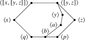
Since all neighbors of $\langle x \rangle $
and
$\langle x \rangle $
and $\langle y \rangle $
are contained in I, we see that
$\langle y \rangle $
are contained in I, we see that $q \in I$
and
$q \in I$
and $a \in I$
, and hence also their common neighbor
$a \in I$
, and hence also their common neighbor $\langle b \rangle $
belongs to I. Now the line
$\langle b \rangle $
belongs to I. Now the line $\langle p, q \rangle $
already contains two points in I (namely
$\langle p, q \rangle $
already contains two points in I (namely $\langle b \rangle $
and
$\langle b \rangle $
and $\langle q \rangle $
), and hence also
$\langle q \rangle $
), and hence also $p \in I$
. Finally, since
$p \in I$
. Finally, since $\langle p \rangle $
and
$\langle p \rangle $
and $\langle [y,z] \rangle $
belong to I, their common neighbor
$\langle [y,z] \rangle $
belong to I, their common neighbor $\langle z \rangle $
belongs to I.
$\langle z \rangle $
belongs to I.
Finally, assume that $(y,z) \in E_2$
, so
$(y,z) \in E_2$
, so $z\in E_2(x)\cap E_2(y)$
. Let
$z\in E_2(x)\cap E_2(y)$
. Let $\langle y\rangle ,\langle a\rangle ,\langle b\rangle ,\langle z\rangle $
be a path of length
$\langle y\rangle ,\langle a\rangle ,\langle b\rangle ,\langle z\rangle $
be a path of length $3$
. If
$3$
. If $\langle a,b\rangle $
is not completely contained in
$\langle a,b\rangle $
is not completely contained in $E_{\leq 1}(x)$
, we can apply the previous paragraph twice to obtain
$E_{\leq 1}(x)$
, we can apply the previous paragraph twice to obtain $z\in I$
. So assumeFootnote 2
$z\in I$
. So assumeFootnote 2 $a,b\in E_1(x)$
(i.e., both a and b are at distance
$a,b\in E_1(x)$
(i.e., both a and b are at distance $2$
from x). Since a generalized hexagon does not contain cycles of length
$2$
from x). Since a generalized hexagon does not contain cycles of length $\leq 5$
, this can only happen if the line
$\leq 5$
, this can only happen if the line $\langle a,b\rangle $
contains a point
$\langle a,b\rangle $
contains a point $\langle c\rangle $
collinear with
$\langle c\rangle $
collinear with $\langle x\rangle $
.
$\langle x\rangle $
.
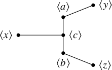
Since $\operatorname {\mathrm {Exp}}(x)$
acts sharply transitively on the set of points of the line
$\operatorname {\mathrm {Exp}}(x)$
acts sharply transitively on the set of points of the line $\langle a, b\rangle $
without
$\langle a, b\rangle $
without $\langle c\rangle $
(see Definition 1.5), we find a unique
$\langle c\rangle $
(see Definition 1.5), we find a unique $\psi \in \operatorname {\mathrm {Exp}}(x)$
such that
$\psi \in \operatorname {\mathrm {Exp}}(x)$
such that $\psi (a) \in \langle b \rangle $
. Let
$\psi (a) \in \langle b \rangle $
. Let $z' := \psi (y)$
, and notice that
$z' := \psi (y)$
, and notice that $\psi $
fixes x. Since
$\psi $
fixes x. Since $x,y \in I$
, also
$x,y \in I$
, also $z' \in I$
. Since
$z' \in I$
. Since $\psi $
fixes x, we get
$\psi $
fixes x, we get $z'\in E_2(x)$
. Now
$z'\in E_2(x)$
. Now $\langle b\rangle = \psi (\langle a\rangle )$
is a neighbor of both
$\langle b\rangle = \psi (\langle a\rangle )$
is a neighbor of both $\langle z\rangle $
and of
$\langle z\rangle $
and of $\langle z'\rangle $
, and thus,
$\langle z'\rangle $
, and thus, $z'\in E_{\leq 1}(z)$
. Since
$z'\in E_{\leq 1}(z)$
. Since $z'\in I$
, the previous paragraph now implies
$z'\in I$
, the previous paragraph now implies $z\in I$
.
$z\in I$
.
We have now shown that $E_2(x) \subseteq I$
, and just as in the case where
$E_2(x) \subseteq I$
, and just as in the case where ${\mathcal {E}}_0 \neq \emptyset $
, we conclude that
${\mathcal {E}}_0 \neq \emptyset $
, we conclude that $I = L$
.
$I = L$
.
Corollary 3.4. Suppose $I_{-1}\neq \emptyset $
. If a nontrivial subspace
$I_{-1}\neq \emptyset $
. If a nontrivial subspace $I \leq L$
satisfies
$I \leq L$
satisfies $[I,y]\leq I$
and
$[I,y]\leq I$
and $[I,I_{-1}]\leq I$
, then
$[I,I_{-1}]\leq I$
, then $I = L$
.
$I = L$
.
Proof. By Lemma 3.3 and the Jacobi identity, I is an ideal of L. Since L is simple, this implies $I=L$
.
$I=L$
.
Another ingredient that we will need is the fact from [Reference Cohen and IvanyosCI07] that if ${\mathcal {E}}_0 \neq \emptyset $
, then each symplectic pair of points induces a subgeometry of the extremal geometry, known as a symplecton. We state the version from [Reference Cuypers and MeulewaeterCM21, Proposition 2.12]. Recall that a polar space is a partial linear space such that for each point p and each line
${\mathcal {E}}_0 \neq \emptyset $
, then each symplectic pair of points induces a subgeometry of the extremal geometry, known as a symplecton. We state the version from [Reference Cuypers and MeulewaeterCM21, Proposition 2.12]. Recall that a polar space is a partial linear space such that for each point p and each line $\ell $
, the point p is collinear with either one or all points of
$\ell $
, the point p is collinear with either one or all points of $\ell $
. A polar space is called nondegenerate if none of its points is collinear with all other points.
$\ell $
. A polar space is called nondegenerate if none of its points is collinear with all other points.
Proposition 3.5 [Reference Cuypers and MeulewaeterCM21, Proposition 2.12 and Lemma 2.18].
Assume that the extremal geometry contains lines and that ${\mathcal {E}}_0 \neq \emptyset $
. Then the extremal geometry contains a collection
${\mathcal {E}}_0 \neq \emptyset $
. Then the extremal geometry contains a collection $\mathcal {S}$
of subspaces such that every pair of points
$\mathcal {S}$
of subspaces such that every pair of points $x,y$
with
$x,y$
with $(x,y)\in {\mathcal {E}}_0$
is contained in a unique element
$(x,y)\in {\mathcal {E}}_0$
is contained in a unique element $S\in \mathcal {S}$
.
$S\in \mathcal {S}$
.
Moreover, for each $S\in \mathcal {S}$
we have
$S\in \mathcal {S}$
we have
-
(i) S is a nondegenerate polar space (of rank
$\geq 2$
, i.e., containing lines). -
(ii) For all points
$x,y\in S$
, we have
$(x,y)\in {\mathcal {E}}_{\leq 0}$
. -
(iii) If a point x is collinear to two non-collinear points of S, then
$x \in S$
. -
(iv) For each point x, the set of points in
${\mathcal {E}}_{\leq -1}(x)\cap S$
is either empty or contains a line. -
(v) If x is a point with
${\mathcal {E}}_2(x) \cap S \neq \emptyset $
, then
$S \cap {\mathcal {E}}_0(x)$
contains a unique point.


The elements of $\mathcal {S}$
are called symplecta.
$\mathcal {S}$
are called symplecta.
We will need the following property of polar spaces.
Lemma 3.6. Let S be a nondegenerate polar space. Let x and y be non-collinear points of S. Then S is generated (as a point-line geometry) by x, y and $x^\perp \cap y^\perp $
, where
$x^\perp \cap y^\perp $
, where $x^\perp $
denotes the set of points collinear with x.
$x^\perp $
denotes the set of points collinear with x.
Proof. Let X be the subspace generated by x, y and $x^\perp \cap y^\perp $
. Since every line through x contains a point collinear to y, we have
$x^\perp \cap y^\perp $
. Since every line through x contains a point collinear to y, we have $x^\perp \subseteq X$
, and similarly
$x^\perp \subseteq X$
, and similarly $y^\perp \subseteq X$
. Consider
$y^\perp \subseteq X$
. Consider $z\in X$
arbitrary. Let
$z\in X$
arbitrary. Let $\ell $
be any line through x. If
$\ell $
be any line through x. If $x^\perp \cap \ell \neq y^\perp \cap \ell $
, then
$x^\perp \cap \ell \neq y^\perp \cap \ell $
, then $\ell \subseteq X$
. So we may assume that
$\ell \subseteq X$
. So we may assume that $\ell $
contains a unique point
$\ell $
contains a unique point $a\in x^\perp \cap y^\perp $
. By the nondegeneracy, we find
$a\in x^\perp \cap y^\perp $
. By the nondegeneracy, we find $b\in x^\perp \cap y^\perp $
such that a and b are not collinear. Now
$b\in x^\perp \cap y^\perp $
such that a and b are not collinear. Now $\ell $
and
$\ell $
and $by$
are opposite lines, and hence, there exists a point c on
$by$
are opposite lines, and hence, there exists a point c on $\ell $
distinct from a which is collinear to a point of
$\ell $
distinct from a which is collinear to a point of $by$
distinct from y and b. Hence, c lies on a line m such that
$by$
distinct from y and b. Hence, c lies on a line m such that $m\cap y^\perp \in by\setminus \{b,y\}$
and thus,
$m\cap y^\perp \in by\setminus \{b,y\}$
and thus, $m\cap y^\perp \neq m\cap x^\perp $
. As before,
$m\cap y^\perp \neq m\cap x^\perp $
. As before, $m\subseteq X$
. In particular,
$m\subseteq X$
. In particular, $c\in X$
, so together with
$c\in X$
, so together with $a\in X$
we obtain
$a\in X$
we obtain $z\in X$
.
$z\in X$
.
The next lemma gives a more precise description of the subspace $L_S$
of L spanned by the elements in S.
$L_S$
of L spanned by the elements in S.
Lemma 3.7. Let S be a symplecton containing x. Then
 $$\begin{align*}L_S=\langle x\rangle \oplus \langle \{\langle z\rangle\in S\mid z\in L_{-1}\}\rangle \oplus \langle \{\langle z\rangle\in S\mid z\in L_{0}\}\rangle. \end{align*}$$
Moreover, $\langle \{\langle z\rangle \in S\mid z\in L_{0}\}\rangle $
is
$\langle \{\langle z\rangle \in S\mid z\in L_{0}\}\rangle $
is $1$
-dimensional.
$1$
-dimensional.
Proof. By Proposition 3.5(v), $S\cap {\mathcal {E}}_0(y)$
consists of a single point
$S\cap {\mathcal {E}}_0(y)$
consists of a single point $\langle z\rangle $
, and since
$\langle z\rangle $
, and since $S \subseteq {\mathcal {E}}_{\leq 0}(x)$
, this implies
$S \subseteq {\mathcal {E}}_{\leq 0}(x)$
, this implies $z \in L_0$
. By Lemma 3.6,
$z \in L_0$
. By Lemma 3.6, $L_S$
is spanned by x, z, and all points
$L_S$
is spanned by x, z, and all points $\langle a\rangle $
collinear to both
$\langle a\rangle $
collinear to both $\langle x\rangle $
and
$\langle x\rangle $
and $\langle z\rangle $
. For such a point
$\langle z\rangle $
. For such a point $\langle a \rangle $
, we have of course
$\langle a \rangle $
, we have of course $a \in E_{-1}(x)$
. Now
$a \in E_{-1}(x)$
. Now $z \in E_{-1}(a) \cap E_0(y)$
, so by Proposition 2.13(iv), we have
$z \in E_{-1}(a) \cap E_0(y)$
, so by Proposition 2.13(iv), we have $(a,y) \not \in E_2$
. Hence,
$(a,y) \not \in E_2$
. Hence, $a \in E_{-1}(x) \cap E_{\leq 1}(y) = L_{-1}$
by Lemma 2.14.
$a \in E_{-1}(x) \cap E_{\leq 1}(y) = L_{-1}$
by Lemma 2.14.
We are now ready to prove the first theorem of this section.
Theorem 3.8. Assume that L is a simple Lie algebra over $k\neq \mathbb F_2$
generated by its pure extremal elements, and assume that the set of lines
$k\neq \mathbb F_2$
generated by its pure extremal elements, and assume that the set of lines $\mathcal {F}$
is nonempty. Consider
$\mathcal {F}$
is nonempty. Consider $x,y\in E$
with
$x,y\in E$
with $g(x,y)=1$
and let
$g(x,y)=1$
and let $L=L_{-2}\oplus L_{-1}\oplus L_0\oplus L_1\oplus L_2$
be the associated
$L=L_{-2}\oplus L_{-1}\oplus L_0\oplus L_1\oplus L_2$
be the associated $5$
-grading. Then both
$5$
-grading. Then both $L_{-1}$
and
$L_{-1}$
and $L_1$
are linearly spanned by the extremal elements contained in it.
$L_1$
are linearly spanned by the extremal elements contained in it.
Proof. As before, let $I_{-1}$
and
$I_{-1}$
and $I_1$
be the subspaces of L linearly spanned by the extremal elements contained in
$I_1$
be the subspaces of L linearly spanned by the extremal elements contained in $L_{-1}$
and
$L_{-1}$
and $L_1$
, respectively. Let
$L_1$
, respectively. Let
 $$\begin{align*}I = \langle x\rangle \oplus I_{-1}\oplus [I_{-1},I_1]\oplus I_1\oplus \langle y \rangle. \end{align*}$$
We will use Corollary 3.4 to show that $I = L$
.
$I = L$
.
We first show that $[I, y] \leq I$
. By Proposition 2.16, we know that
$[I, y] \leq I$
. By Proposition 2.16, we know that $[x,y]\in [I_{-1},I_1]$
. Next, if
$[x,y]\in [I_{-1},I_1]$
. Next, if $a\in E\cap L_{-1}$
, then
$a\in E\cap L_{-1}$
, then $a\in E_1(y)$
, and hence,
$a\in E_1(y)$
, and hence, $[a,y]\in I_{1}$
. Since
$[a,y]\in I_{1}$
. Since $[L_{\geq 0}, y] \leq L_2 = \langle y \rangle $
, the claim
$[L_{\geq 0}, y] \leq L_2 = \langle y \rangle $
, the claim $[I,y]\leq I$
is now clear.
$[I,y]\leq I$
is now clear.
It remains to show that $[I,I_{-1}]\leq I$
. Obviously,
$[I,I_{-1}]\leq I$
. Obviously, $[\langle x\rangle \oplus I_{-1}\oplus I_1,I_{-1}]\leq I$
. Similarly as before,
$[\langle x\rangle \oplus I_{-1}\oplus I_1,I_{-1}]\leq I$
. Similarly as before, $[\langle y\rangle ,I_{-1}]\leq I_1\leq I$
, so the only case left to prove is
$[\langle y\rangle ,I_{-1}]\leq I_1\leq I$
, so the only case left to prove is
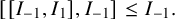 $$\begin{align*}[[I_{-1},I_1],I_{-1}]\leq I_{-1}. \end{align*}$$
So consider arbitrary extremal elements $a,b\in E\cap L_{-1}$
and
$a,b\in E\cap L_{-1}$
and $c\in E\cap L_1$
; our goal is to show that
$c\in E\cap L_1$
; our goal is to show that
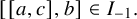 $$ \begin{align} [[a,c],b]\in I_{-1}. \end{align} $$
Observe that $[a,b] \in L_{-2} = \langle x \rangle $
, so by the Jacobi identity and the fact that
$[a,b] \in L_{-2} = \langle x \rangle $
, so by the Jacobi identity and the fact that $[x,c]$
is contained in
$[x,c]$
is contained in $E\cap L_{-1}$
, we have
$E\cap L_{-1}$
, we have
 $$\begin{align*}[[a,c], b] \in I_{-1} \iff [[b,c], a] \in I_{-1}. \end{align*}$$
Also observe that $c\in E_{\leq 0}(a)$
implies
$c\in E_{\leq 0}(a)$
implies $[a,c]=0$
and that
$[a,c]=0$
and that $c\in E_{\leq 0}(b)$
implies
$c\in E_{\leq 0}(b)$
implies $[b,c]=0$
. Hence, we may assume from now on that
$[b,c]=0$
. Hence, we may assume from now on that $c\in E_{\geq 1}(a)\cap E_{\geq 1}(b)$
.
$c\in E_{\geq 1}(a)\cap E_{\geq 1}(b)$
.
Since a is extremal, $[[a,c], a] \in \langle a \rangle $
is again extremal, so (6) obviously holds if
$[[a,c], a] \in \langle a \rangle $
is again extremal, so (6) obviously holds if $(a,b) \in E_{-2}$
. If
$(a,b) \in E_{-2}$
. If $(a,b) \in E_{-1}$
, then by [Reference Cuypers and MeulewaeterCM21, Lemma 6.3],
$(a,b) \in E_{-1}$
, then by [Reference Cuypers and MeulewaeterCM21, Lemma 6.3], $J := \langle a,b\rangle $
is an inner ideal (i.e.,
$J := \langle a,b\rangle $
is an inner ideal (i.e., $[J, [J, L]] \leq J$
); in particular,
$[J, [J, L]] \leq J$
); in particular, $[b,[a,c]] \in J \leq I_{-1}$
. Next, if
$[b,[a,c]] \in J \leq I_{-1}$
. Next, if $(a,b) \in E_{0}$
, then a and b are contained in a symplecton S. The subspace
$(a,b) \in E_{0}$
, then a and b are contained in a symplecton S. The subspace $L_S$
spanned by all elements of S is an inner ideal by [Reference Cuypers and MeulewaeterCM21, Lemma 6.5], and hence,
$L_S$
spanned by all elements of S is an inner ideal by [Reference Cuypers and MeulewaeterCM21, Lemma 6.5], and hence, $[b,[a,c]]\in L_S$
. Since
$[b,[a,c]]\in L_S$
. Since $[b,[a,c]]\in L_{-1}$
, Lemma 3.7 now implies that
$[b,[a,c]]\in L_{-1}$
, Lemma 3.7 now implies that $[b,[a,c]] \in \langle \{ \langle z\rangle \in S\mid z\in L_{-1}\} \rangle \leq I_{-1}$
.
$[b,[a,c]] \in \langle \{ \langle z\rangle \in S\mid z\in L_{-1}\} \rangle \leq I_{-1}$
.
Now notice that $(a,b) \in E_2$
cannot occur because both a and b are collinear to x, so we can assume from now on that
$(a,b) \in E_2$
cannot occur because both a and b are collinear to x, so we can assume from now on that $(a,b) \in E_1$
. In particular,
$(a,b) \in E_1$
. In particular, $[a,b] \in \langle x \rangle \setminus \{ 0 \}$
.
$[a,b] \in \langle x \rangle \setminus \{ 0 \}$
.
If $c\in E_1(a)$
, then
$c\in E_1(a)$
, then $[a,c]\in E$
, and since the extremal form g is associative, we have
$[a,c]\in E$
, and since the extremal form g is associative, we have $g(b,[a,c])=g([b,a],c)=0$
, since
$g(b,[a,c])=g([b,a],c)=0$
, since $c\in E_1(x)$
. Hence,
$c\in E_1(x)$
. Hence, $[a,c]\in E_{\leq 1}(b)$
, so either
$[a,c]\in E_{\leq 1}(b)$
, so either $[[a,c],b]\in E$
or
$[[a,c],b]\in E$
or $[[a,c],b]=0$
. In either case, we obtain
$[[a,c],b]=0$
. In either case, we obtain $[[a,c],b]\in I_{-1}$
. The case
$[[a,c],b]\in I_{-1}$
. The case $c\in E_1(b)$
is similar.
$c\in E_1(b)$
is similar.
The only case left to consider is $a\in E_1(b)$
and
$a\in E_1(b)$
and $c\in E_2(a)\cap E_2(b)$
, and this case requires some more effort. We have
$c\in E_2(a)\cap E_2(b)$
, and this case requires some more effort. We have $g(a,b)=0$
, and by rescaling, we may assume that
$g(a,b)=0$
, and by rescaling, we may assume that $g(a,c) = g(b,c) = 1$
, and we also have
$g(a,c) = g(b,c) = 1$
, and we also have $g(b, [a,c]) = 0$
as before.
$g(b, [a,c]) = 0$
as before.
Let $\lambda ,\mu \in k$
be arbitrary nonzero elements such that
$\lambda ,\mu \in k$
be arbitrary nonzero elements such that
 $$ \begin{align} \mu (\lambda - 1) = 1 , \end{align} $$
which exist because $k \neq \mathbb F_2$
, and consider the extremal element
$k \neq \mathbb F_2$
, and consider the extremal element
 $$\begin{align*}d := \exp(\mu c)\exp(\lambda b)\exp(c)(a) .\end{align*}$$
Then
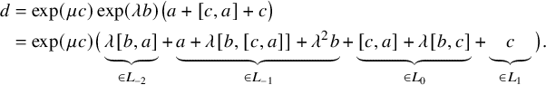 $$ \begin{align*} d &= \exp(\mu c)\exp(\lambda b) \big(a + [c,a] + c \big) \\ &= \exp(\mu c) \big( \underbrace{\lambda [b,a]}_{\in L_{-2}} + \underbrace{a + \lambda [b, [c,a]] + \lambda^2 b}_{\in L_{-1}} + \underbrace{[c,a] + \lambda [b,c]}_{\in L_0} + \underbrace{c\vphantom{[]}}_{\in L_1} \big). \end{align*} $$
We claim that $d \in L_{\leq -1}$
. This could be checked by a direct computation, but it is easier to reverse the process, by starting from an arbitrary extremal element of the form
$d \in L_{\leq -1}$
. This could be checked by a direct computation, but it is easier to reverse the process, by starting from an arbitrary extremal element of the form
 $$\begin{align*}e := \lambda [b,a] + z \in \langle x \rangle + L_{-1} , \end{align*}$$
compute $\exp (-\mu c)(e)$
, and verify that with the correct choice of z, this is equal to
$\exp (-\mu c)(e)$
, and verify that with the correct choice of z, this is equal to $\exp (-\mu c)(d)$
. We get
$\exp (-\mu c)(d)$
. We get
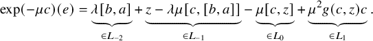 $$\begin{align*}\exp(-\mu c)(e) = \underbrace{\lambda [b,a]}_{\in L_{-2}} + \underbrace{z - \lambda \mu [c,[b,a]]}_{\in L_{-1}} - \underbrace{\mu [c,z]}_{\in L_0} + \underbrace{\mu^2 g(c,z)c\vphantom{[]}}_{\in L_1}. \end{align*}$$
Comparing the $L_{-1}$
-components, we have no other choice than setting
$L_{-1}$
-components, we have no other choice than setting
 $$ \begin{align} z := a + \lambda^2 b + \lambda [b,[c,a]] + \lambda \mu [c,[b,a]]. \end{align} $$
Now, using the Premet identity (3) (see Definition 1.2) and the fact that $g(c, [b,a]) = 0$
, we get
$g(c, [b,a]) = 0$
, we get
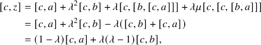 $$ \begin{align*} [c,z] &= [c,a] + \lambda^2 [c,b] + \lambda [c,[b,[c,a]]] + \lambda \mu [c,[c,[b,a]]] \\ &= [c,a] + \lambda^2 [c,b] - \lambda ([c,b] + [c,a]) \\ &= (1 - \lambda) [c,a] + \lambda (\lambda - 1) [c,b], \end{align*} $$
and hence by (7), $-\mu [c,z] = [c,a] - \lambda [c,b]$
, so the
$-\mu [c,z] = [c,a] - \lambda [c,b]$
, so the $L_0$
-components coincide. Finally,
$L_0$
-components coincide. Finally,
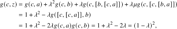 $$ \begin{align*} g(c,z) &= g(c,a) + \lambda^2 g(c,b) + \lambda g(c,[b,[c,a]]) + \lambda \mu g(c,[c,[b,a]]) \\ &= 1 + \lambda^2 - \lambda g([c, [c, a]], b) \\ &= 1 + \lambda^2 - 2 \lambda g(c,a) g(c, b) = 1 + \lambda^2 - 2 \lambda = (1 - \lambda)^2 , \end{align*} $$
so again by (7), $\mu ^2 g(c,z)= 1$
, and hence also the
$\mu ^2 g(c,z)= 1$
, and hence also the $L_1$
-components coincide. Therefore,
$L_1$
-components coincide. Therefore, $e=d$
, and we conclude that the element
$e=d$
, and we conclude that the element $e = \lambda [b,a] + z \in \langle x \rangle + L_{-1}$
is an extremal element.
$e = \lambda [b,a] + z \in \langle x \rangle + L_{-1}$
is an extremal element.
If $z = 0$
, then by (8),
$z = 0$
, then by (8), $[b,[c,a]]$
can be written as the sum of
$[b,[c,a]]$
can be written as the sum of $3$
extremal elements contained in
$3$
extremal elements contained in $L_{-1}$
. Indeed, obviously
$L_{-1}$
. Indeed, obviously $a, b\in E$
, but also
$a, b\in E$
, but also $[c,[b,a]]\in E$
since
$[c,[b,a]]\in E$
since $\langle c\rangle $
and
$\langle c\rangle $
and $\langle x\rangle =\langle [b,a]\rangle $
form a special pair.
$\langle x\rangle =\langle [b,a]\rangle $
form a special pair.
If $z \neq 0$
, then
$z \neq 0$
, then $\langle e,x \rangle $
is a line of the extremal geometry. Since
$\langle e,x \rangle $
is a line of the extremal geometry. Since $z \in \langle e,x\rangle $
, it is contained in E. So by (8) again, the element
$z \in \langle e,x\rangle $
, it is contained in E. So by (8) again, the element $[b,[c,a]]$
can be written as the sum of
$[b,[c,a]]$
can be written as the sum of $4$
extremal elements contained in
$4$
extremal elements contained in $L_{-1}$
.
$L_{-1}$
.
This shows that $[b,[c,a]] \in I_{-1}$
in all possible cases.
$[b,[c,a]] \in I_{-1}$
in all possible cases.
Now we will work toward showing the so-called algebraicity of the Lie algebra, using the previous theorem. We will give a precise definition of this property in Definition 3.15 below, but loosely speaking, it means that for any element in $L_{-1}$
, there exist automorphisms depending on this element which behave nicely with respect to the
$L_{-1}$
, there exist automorphisms depending on this element which behave nicely with respect to the $5$
-grading. Actually, if the characteristic is not
$5$
-grading. Actually, if the characteristic is not $2$
,
$2$
, $3$
or
$3$
or $5$
, this property is easily shown (recall the discussion following Definition 1.10), so it is not surprising that we sometimes have to handle the small characteristic cases a bit more carefully.
$5$
, this property is easily shown (recall the discussion following Definition 1.10), so it is not surprising that we sometimes have to handle the small characteristic cases a bit more carefully.
In the next two lemmas, we show that as soon as an extremal element has a certain form, it is contained in the image of a specific element under $\operatorname {\mathrm {Exp}}(x)$
. We will use this later to show the uniqueness of certain automorphisms.
$\operatorname {\mathrm {Exp}}(x)$
. We will use this later to show the uniqueness of certain automorphisms.
Lemma 3.9. Assume $\operatorname {\mathrm {char}}(k)\neq 3$
. Let
$\operatorname {\mathrm {char}}(k)\neq 3$
. Let $l=l_{-2}+l_{-1}+e$
be an extremal element, with
$l=l_{-2}+l_{-1}+e$
be an extremal element, with $l_i \in L_i$
and
$l_i \in L_i$
and $e\in E\cap L_1$
. Then
$e\in E\cap L_1$
. Then $l_{-2} = 0$
and
$l_{-2} = 0$
and $l_{-1} \in \langle [x,e] \rangle $
. In particular,
$l_{-1} \in \langle [x,e] \rangle $
. In particular, $l=\exp (\lambda x)(e) = e + \lambda [x,e]$
for some
$l=\exp (\lambda x)(e) = e + \lambda [x,e]$
for some $\lambda \in k$
.
$\lambda \in k$
.
Proof. By Proposition 2.4(ii), we have
 $$\begin{align*}[l,[l,[x,y]]]=[l,2l_{-2}+l_{-1}-e]=-3[l_{-2},e]-2[l_{-1},e] \in L_{-1} + L_0.\end{align*}$$
However, since l is extremal, we have $[l, [l, [x,y]]] \in \langle l \rangle $
. By the previous identity, this element must have trivial
$[l, [l, [x,y]]] \in \langle l \rangle $
. By the previous identity, this element must have trivial $L_1$
-component, but since
$L_1$
-component, but since $e \neq 0$
by assumption, this implies that
$e \neq 0$
by assumption, this implies that $[l, [l, [x,y]]] = 0$
, so
$[l, [l, [x,y]]] = 0$
, so
 $$\begin{align*}3[l_{-2}, e] = 2[l_{-1}, e] = 0. \end{align*}$$
Since $\operatorname {\mathrm {char}}(k) \neq 3$
, this implies
$\operatorname {\mathrm {char}}(k) \neq 3$
, this implies $[l_{-2},e]=0$
, and hence,
$[l_{-2},e]=0$
, and hence, $l_{-2}=0$
by Proposition 2.4(iii). If
$l_{-2}=0$
by Proposition 2.4(iii). If $l_{-1}=0$
, then there is nothing to show, so assume
$l_{-1}=0$
, then there is nothing to show, so assume $l_{-1}\neq 0$
. Then
$l_{-1}\neq 0$
. Then
 $$\begin{align*}l = l_{-1} + e \in L_{-1} + L_1 , \quad l_{-1} \neq 0, \quad e \neq 0. \end{align*}$$
By Proposition 2.5, we have $l\in E_1(y)$
, and thus,
$l\in E_1(y)$
, and thus, $[l_{-1},y] = [l,y] \in E$
. By Proposition 2.5 again,
$[l_{-1},y] = [l,y] \in E$
. By Proposition 2.5 again, $[l_{-1},y]\in E_1(x)$
, and thus,
$[l_{-1},y]\in E_1(x)$
, and thus, $l_{-1}=[x,[l_{-1},y]]\in E$
. Since
$l_{-1}=[x,[l_{-1},y]]\in E$
. Since $l_{-1}$
, e and
$l_{-1}$
, e and $l=l_{-1}+e$
are contained in E, Proposition 1.8 implies that
$l=l_{-1}+e$
are contained in E, Proposition 1.8 implies that $(l_{-1},e)\in E_{-1}$
. Hence,
$(l_{-1},e)\in E_{-1}$
. Hence, $\langle l_{-1}\rangle $
is the common neighbor of the special pair
$\langle l_{-1}\rangle $
is the common neighbor of the special pair $(\langle x\rangle , \langle e\rangle )$
, and thus,
$(\langle x\rangle , \langle e\rangle )$
, and thus, $l_{-1}\in \langle [x,e]\rangle $
.
$l_{-1}\in \langle [x,e]\rangle $
.
Lemma 3.10. Let $l=l_{-2}+l_{-1}+l_0+y\in E$
be an extremal element, with
$l=l_{-2}+l_{-1}+l_0+y\in E$
be an extremal element, with $l_i \in L_i$
. Then
$l_i \in L_i$
. Then $l_{-1} = 0$
and
$l_{-1} = 0$
and $l=\exp (\lambda x)(y)$
for some
$l=\exp (\lambda x)(y)$
for some $\lambda \in k$
.
$\lambda \in k$
.
Proof. Let $\lambda ,\mu \in k$
be such that
$\lambda ,\mu \in k$
be such that $l_{-2}=\lambda x$
and
$l_{-2}=\lambda x$
and $[l_0,x]=\mu x$
. By Proposition 2.4(ii), we have
$[l_0,x]=\mu x$
. By Proposition 2.4(ii), we have
 $$ \begin{align*} [l,[l,x]] &= [l, \mu x + [y,x]] \\ &= \mu [l,x] + \big[ \lambda x+l_{-1}+l_0+y, [y,x] \big] \\ &= (\mu^2 x+\mu[y,x])+(-2\lambda x-l_{-1}+2y). \end{align*} $$
Since l is extremal and $g(l, x) = g(y, x)=1$
by Proposition 2.4(v), we get
$g(l, x) = g(y, x)=1$
by Proposition 2.4(v), we get
 $$ \begin{align} \mu^2 = 4\lambda, \quad 3 l_{-1} = 0, \quad \mu[y,x]=2l_0. \end{align} $$
If $\operatorname {\mathrm {char}}(k)$
is not
$\operatorname {\mathrm {char}}(k)$
is not $2$
or
$2$
or $3$
, then this already implies that
$3$
, then this already implies that $l =\exp (-\tfrac {1}{2} \mu x)(y)$
.
$l =\exp (-\tfrac {1}{2} \mu x)(y)$
.
Assume now $\operatorname {\mathrm {char}}(k)=3$
. We claim that also in this case,
$\operatorname {\mathrm {char}}(k)=3$
. We claim that also in this case, $l_{-1} = 0$
; it then follows again that
$l_{-1} = 0$
; it then follows again that $l=\exp (-\tfrac {1}{2} \mu x)(y)$
. To show the claim, suppose that
$l=\exp (-\tfrac {1}{2} \mu x)(y)$
. To show the claim, suppose that $l_{-1} \neq 0$
and let
$l_{-1} \neq 0$
and let $z := \exp (\tfrac {1}{2} \mu x)(l)$
. Then z is an extremal element, and we compute that
$z := \exp (\tfrac {1}{2} \mu x)(l)$
. Then z is an extremal element, and we compute that $z = l_{-1} + y$
. We apply the same technique as in the last paragraph of the proof of Lemma 3.9: By Proposition 2.5,
$z = l_{-1} + y$
. We apply the same technique as in the last paragraph of the proof of Lemma 3.9: By Proposition 2.5, $z \in E_1(y)$
, and thus,
$z \in E_1(y)$
, and thus, $[l_{-1},y] = [z,y] \in E$
. By Proposition 2.5 again,
$[l_{-1},y] = [z,y] \in E$
. By Proposition 2.5 again, $[l_{-1}, y]\in E_1(x)$
, and thus,
$[l_{-1}, y]\in E_1(x)$
, and thus, $l_{-1} = [x, [l_{-1}, y]] \in E$
. Since
$l_{-1} = [x, [l_{-1}, y]] \in E$
. Since $l_{-1}$
, y and
$l_{-1}$
, y and $z = l_{-1}+y$
are contained in E, Proposition 1.8 implies that
$z = l_{-1}+y$
are contained in E, Proposition 1.8 implies that $(l_{-1}, y) \in E_{-1}$
, contradicting Proposition 2.5.
$(l_{-1}, y) \in E_{-1}$
, contradicting Proposition 2.5.
Assume, finally, that $\operatorname {\mathrm {char}}(k)=2$
. By (9), we have
$\operatorname {\mathrm {char}}(k)=2$
. By (9), we have $l_{-1}=0$
, so
$l_{-1}=0$
, so $l \in L_{-2} + L_0 + L_2$
. By Proposition 2.16, there exist
$l \in L_{-2} + L_0 + L_2$
. By Proposition 2.16, there exist $c,d \in E\cap L_{-1}$
such that
$c,d \in E\cap L_{-1}$
such that $[c, d] = x$
. By Lemma 2.15, we get for any
$[c, d] = x$
. By Lemma 2.15, we get for any $e\in E\cap L_{-1}$
that
$e\in E\cap L_{-1}$
that $g(l,e)=0$
, and since
$g(l,e)=0$
, and since $[y,e]\neq 0$
, this implies that the pair
$[y,e]\neq 0$
, this implies that the pair $(l,e)$
is special; in particular,
$(l,e)$
is special; in particular, $[l,e] = [l_0,e] + [y,e] \in L_{-1} + L_1$
is extremal. By Lemma 3.9 applied on
$[l,e] = [l_0,e] + [y,e] \in L_{-1} + L_1$
is extremal. By Lemma 3.9 applied on $[l,c]$
and
$[l,c]$
and $[l,d]$
, we find
$[l,d]$
, we find $\lambda ,\mu \in k$
such that
$\lambda ,\mu \in k$
such that $[l_0, c] = \lambda [x, [y, c]] = \lambda c$
and
$[l_0, c] = \lambda [x, [y, c]] = \lambda c$
and $[l_0, d] = \mu [x, [y, d]] = \mu d$
. Let
$[l_0, d] = \mu [x, [y, d]] = \mu d$
. Let $\alpha := \exp (\lambda x)$
. Then
$\alpha := \exp (\lambda x)$
. Then
 $$\begin{align*}\alpha([l,c])=[y,c], \quad \alpha([l,d])=[y,d] + (\lambda + \mu) d. \end{align*}$$
By the Premet identity (2), we have
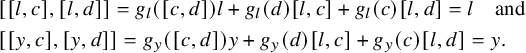 $$ \begin{align*} &[[l,c],[l,d]] = g_l ([c,d])l + g_l (d)[l,c] + g_{l}(c)[l,d] = l \quad \text{and} \\ &[[y,c],[y,d]] = g_y ([c,d])y + g_y (d)[l,c] + g_{y}(c)[l,d] = y. \end{align*} $$
Hence,
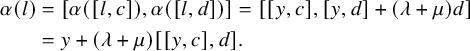 $$ \begin{align*} \alpha(l) &= [\alpha([l,c]),\alpha([l,d])]=[[y,c], [y,d] + (\lambda + \mu)d] \\ &= y + (\lambda + \mu) [[y, c], d]. \end{align*} $$
Now note that by the Premet identity (3), we have
 $$\begin{align*}[y, [d, [y, c]]] = g_y([d,c]) y + g_y(c) [y,d] + g_y(d) [y,c] = y, \end{align*}$$
and hence,
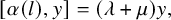 $$\begin{align*}[\alpha(l), y] = (\lambda + \mu) y , \end{align*}$$
but then since $\operatorname {\mathrm {char}}(k) = 2$
and
$\operatorname {\mathrm {char}}(k) = 2$
and $\alpha (l)$
is an extremal element, we get
$\alpha (l)$
is an extremal element, we get
 $$\begin{align*}0 = [\alpha(l), [\alpha(l), y]] = (\lambda + \mu)^2 y , \end{align*}$$
so $\lambda = \mu $
and therefore
$\lambda = \mu $
and therefore $\alpha (l) = y$
and so
$\alpha (l) = y$
and so $l = \alpha (y)$
(since
$l = \alpha (y)$
(since $\alpha ^2 = 1$
).
$\alpha ^2 = 1$
).
Definition 3.11. Assume that the extremal geometry of L has lines. We set
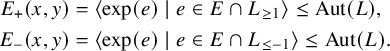 $$ \begin{align*} E_+(x,y) &= \langle \exp(e) \mid e\in E \cap L_{\geq 1} \rangle\leq \operatorname{\mathrm{Aut}}(L), \\ E_-(x,y) &= \langle \exp(e) \mid e\in E \cap L_{\leq -1} \rangle\leq \operatorname{\mathrm{Aut}}(L). \end{align*} $$
It is important to point out that these groups are generated by elements of the form $\exp (e)$
and that an arbitrary element of
$\exp (e)$
and that an arbitrary element of $E_\pm (x,y)$
cannot be written as a single
$E_\pm (x,y)$
cannot be written as a single $\exp (e)$
in general. In Definition 3.15 below, we will give a different definition of the groups
$\exp (e)$
in general. In Definition 3.15 below, we will give a different definition of the groups $E_\pm (x,y)$
that also makes sense when the extremal geometry has no lines.
$E_\pm (x,y)$
that also makes sense when the extremal geometry has no lines.
The following theorem is the key tool in our paper. It allows us to deal with exponential maps even in characteristic $2$
and
$2$
and $3$
.
$3$
.
Definition 3.12. Let $\alpha \in \operatorname {\mathrm {Aut}}(L)$
and
$\alpha \in \operatorname {\mathrm {Aut}}(L)$
and $l \in L_1$
. We say that
$l \in L_1$
. We say that $\alpha $
is an l-exponential automorphism if there exist (necessarily unique) maps
$\alpha $
is an l-exponential automorphism if there exist (necessarily unique) maps $q_{\alpha },n_{\alpha },v_{\alpha } \colon L \to L$
with
$q_{\alpha },n_{\alpha },v_{\alpha } \colon L \to L$
with
 $$ \begin{align} q_{\alpha}(L_i)\subseteq L_{i+2}, \quad n_{\alpha}(L_i)\subseteq L_{i+3}, \quad v_{\alpha}(L_i)\subseteq L_{i+4}, \end{align} $$
for all $i\in [-2,2]$
, such that
$i\in [-2,2]$
, such that
 $$ \begin{align} \alpha(m)=m+[l,m]+q_{\alpha}(m)+n_{\alpha}(m)+v_{\alpha}(m) \end{align} $$
for all $m\in L$
.
$m\in L$
.
Theorem 3.13. Assume that L is a simple Lie algebra over $k\neq \mathbb F_2$
generated by its pure extremal elements, and assume that
$k\neq \mathbb F_2$
generated by its pure extremal elements, and assume that $\mathcal {F}\neq \emptyset $
. Consider a hyperbolic pair
$\mathcal {F}\neq \emptyset $
. Consider a hyperbolic pair $x,y\in E$
with
$x,y\in E$
with $g(x,y)=1$
and let
$g(x,y)=1$
and let $L=L_{-2}\oplus L_{-1}\oplus L_0\oplus L_1\oplus L_2$
be the associated
$L=L_{-2}\oplus L_{-1}\oplus L_0\oplus L_1\oplus L_2$
be the associated $5$
-grading. Then
$5$
-grading. Then
-
(i)
$\exp (a)\exp (b) = \exp ([a,b])\exp (b)\exp (a)$
for all
$a,b \in E \cap L_{\geq 1}$
. -
(ii)
$\exp (a)\exp (b) = \exp (a+b)$
for all
$a \in E \cap L_{\geq 1}$
and
$b \in L_2$
. -
(iii)
$[E_+(x,y), E_+(x,y)] = \operatorname {\mathrm {Exp}}(y)$
and
$[E_+(x,y), \operatorname {\mathrm {Exp}}(y)] = 1$
.


Assume now that $l \in L_1$
.
$l \in L_1$
.
-
(iv) Write
$l = e_1 + \dots + e_n$
with
$e_i \in E \cap L_1$
. Then is an l-exponential automorphism.
$$\begin{align*}\alpha := \exp(e_1) \dotsm \exp(e_n) \in E_+(x,y) \end{align*}$$
-
(v) If
$\alpha $
is as in (iv) and
$\beta $
is another l-exponential automorphism, then
$\beta = \exp (z)\alpha $
for a unique
$z\in L_{2}$
. In particular,
$\beta \in E_+(x,y)$
. -
(vi) Let
$\alpha $
be any l-exponential automorphism. Then there exist
$e_1,\dots ,e_n \in E \cap L_1$
such that
$l = e_1 + \dots + e_n$
and
$\alpha = \exp (e_1) \dotsm \exp (e_n)$
. Moreover,
$$\begin{align*}E_+(x,y) = \big\{ \alpha\in \operatorname{\mathrm{Aut}}(L)\mid \alpha \text{ is }m\text{-exponential for some } m \in L_{1} \big\}. \end{align*}$$
-
(vii) Let
$\alpha $
be an l-exponential automorphism, with maps
$q_{\alpha }, n_{\alpha }, v_{\alpha } \colon L \to L$
. Then for each
$\lambda \in k$
, the map
$\alpha _{\lambda }$
defined by for all
$$\begin{align*}\alpha_{\lambda}(m)=m+\lambda[l,m]+\lambda^2q_{\alpha}(m)+\lambda^3n_{\alpha}(m)+\lambda^4v_{\alpha}(m) \end{align*}$$
$m\in L$
, is a
$(\lambda l)$
-exponential automorphism. In particular,
$\alpha _\lambda \in E_+(x,y)$
.
-
(viii) If
$\alpha $
is an l-exponential automorphism and
$\beta $
is an
$l'$
-exponential automorphism, then
$\alpha \beta $
is an
$(l+l')$
-exponential automorphism. -
(ix) If
$\operatorname {\mathrm {char}} (k)\neq 2$
, then there is a unique l-exponential automorphism
$\alpha $
with
$q_{\alpha }(m) = \tfrac {1}{2} [l,[l,m]]$
for all
$m \in L$
. We denote this automorphism by
$e_+(l)$
. Its inverse is
$e_+(-l)$
.


Proof.
-
(i) Let
$a,b\in E \cap L_{\geq 1}$
; notice that
$g(a,b)=0$
. Since L is generated by
$L_{\geq -1}$
, it suffices to check that both sides coincide when applied on an element
$l \in L_{\geq -1}$
. We have (12)
$$ \begin{align} \exp(a)\exp(b)(l) &= \exp(a)\big( l + [b,l] + g(b,l)b \big) \nonumber \\ &= l + [a+b, l] + [a,[b,l]] \nonumber \\ &+ g([a,b],l)a + g(b,l)[a,b] + g(a,l)a + g(b,l)b. \end{align} $$
Using the Premet identity (3), we have
(13)
$$ \begin{align} [[a,b],[a+b,l]] &= [[a,b],[a,l]]-[[b,a],[b,l]] \nonumber \\ &= g_a([b,l])a+g_a(l)[a,b]-g_a(b)[a,l]\nonumber\\ & -g_b([a,l])b-g_b(l)[b,a]+g_b(a)[b,l]\nonumber\\ &= g([a,b],l)a + g([a,b],l)b + (g(a,l)+g(b,l))[a,b]. \end{align} $$
Since
$[a,b]\in L_2$
, the automorphism
$\exp ([a,b])$
fixes all elements of
$L_{\geq 1}$
. Hence, by (12) with the roles of a and b reversed, (13) and the Jacobi identity, we see that as claimed.
$$\begin{align*}\exp(a)\exp(b)(l)=\exp([a,b])\exp(b)\exp(a)(l), \end{align*}$$
-
(ii) We again check that both sides coincide when applied on an element
$l \in L_{\geq -1}$
. Comparing (12) with the expression for
$\exp (a+b)(l)$
and using the fact that
$[a,b] = 0$
and that b is a multiple of y, we see that this is equivalent with
$$\begin{align*}[a, [y, l]] = g(a,l)y + g(y,l)a. \end{align*}$$
Now both sides are equal to
$0$
if
$l \in L_{\geq 0}$
. Furthermore, if
$l \in L_{-2}$
, then we can write
$l = \lambda x$
with
$\lambda \in k$
to see that both sides are equal to
$\lambda a$
, and if
$l \in L_{-1}$
, then the equality follows from Lemma 2.7. -
(iii) By (i), we already know that
$[E_+(x,y),E_+(x,y)]\leq \operatorname {\mathrm {Exp}}(y)$
. By Proposition 2.16, the element y can be written as
$y = [c,d]$
for certain
$c,d \in E \cap L_1$
. By (i) again, we see that
$\exp ([c,d]) \in [E_+(x,y),E_+(x,y)]$
, and by rescaling, we get
$\operatorname {\mathrm {Exp}}(y) \leq [E_+(x,y),E_+(x,y)]$
, as required. The second statement follows immediately from (i) since
$[a,b] = 0$
if
$b \in L_2$
. -
(iv) Let
$l\in L_1$
. By Theorem 3.8, we can write l as the sum of a finite number of extremal elements in
$L_1$
:
$$\begin{align*}l = e_1+\dots+e_n \quad \text{with } e_i\in E\cap L_1. \end{align*}$$
We will prove, by induction on n, that the automorphism
satisfies (10) and (11) for the appropriate choices of maps
$$\begin{align*}\alpha := \exp(e_1) \dotsm \exp(e_n) \in E_+(x,y) \end{align*}$$
$q_\alpha $
,
$n_\alpha $
and
$v_\alpha $
. (Notice that
$\alpha $
depends on the choice of the elements
$e_1,\dots ,e_n$
as well as on their ordering.)
If
$n=1$
, then we set for all
$$\begin{align*}q_{\alpha}(m) := g_l(m)l, \quad n_{\alpha}(m) := 0, \quad v_{\alpha}(m) := 0 , \end{align*}$$
$m \in L$
. By Definition 1.5, we see that (11) is satisfied. By Lemma 2.15,
$q_\alpha (L_i) = 0$
unless
$i = -1$
, so (10) holds as well.
Now assume
$n>1$
, let
$e := e_1$
and let
$l'=e_2+\dots +e_n$
, so
$l = e + l'$
. Let
$\alpha ' := \exp (e_2) \dotsm \exp (e_n)$
, so
$\alpha := \exp (e)\alpha '$
. By the induction hypothesis, there exist maps
$q_{\alpha '}, n_{\alpha '}$
and
$v_{\alpha '}$
satisfying (10) and (11). We set (14)
$$ \begin{align}e q_{\alpha}(m) &:= q_{\alpha'}(m)+g_{e}(m)e+[e,[l',m]],\end{align} $$
(15)
$$ \begin{align} n_{\alpha}(m) &:= n_{\alpha'}(m)+g_{e}([l',m])e+[e,q_{\alpha'}(m)], \end{align} $$
(16)for all
$$ \begin{align} v_{\alpha}(m) &:= v_{\alpha'}(m)+[e,n_{\alpha'}(m)],\qquad\qquad \end{align} $$
$m\in L$
. By Lemma 2.15 and the fact that (10) holds for
$\alpha '$
, we get for all
$$ \begin{align*} &[e,v_{\alpha'}(m)]\in L_{\geq (1+4-2)}=L_{\geq 3}=0 \quad \text{and} \\ &g_{e}(q_{\alpha'}(m))=g_{e}(n_{\alpha'}(m))=g_{e}(v_{\alpha'}(m))=0 \end{align*} $$
$m \in L$
, and by expanding using the fact that (11) holds for
$$\begin{align*}\alpha(m) = \exp(e)(\alpha'(m)) = \alpha'(m) + [e, \alpha'(m)] + g_e(\alpha'(m)) e, \end{align*}$$
$\alpha '$
, we now see that (11) is satisfied for
$\alpha $
. By Lemma 2.15 again, we see that also (10) holds for
$\alpha $
.
-
(v) Let
$l \in L_1$
and let
$\beta \in \operatorname {\mathrm {Aut}}(L)$
be any automorphism satisfying (10) and (11). Let
$\alpha $
be the automorphism
$\alpha = \exp (e_1) \dotsm \exp (e_n)$
as constructed in (iv) with respect to some choice
$l = e_1 + \dots + e_n$
, and observe that by the same construction, then satisfies (10) and (11) for the element
$$\begin{align*}\alpha^{-1} = \exp(-e_n) \dotsm \exp(-e_1) \end{align*}$$
$-l = -e_n - \dots - e_1$
.
Now
$\alpha $
and
$\beta $
coincide on
$L_{\geq 1}$
. However, any element of
$E_+(x,y)$
preserves the filtration
$(L_{\geq i})$
, so in particular,
$\alpha ^{-1}(L_{\geq 1}) = L_{\geq 1}$
. Hence,
$\alpha \alpha ^{-1}$
and
$\beta \alpha ^{-1}$
coincide on
$L_{\geq 1}$
, so
$\gamma := \beta \alpha ^{-1}$
fixes
$L_{\geq 1}$
.Moreover, by (11) for
$\beta $
and
$\alpha ^{-1}$
, we have so
$$\begin{align*}\gamma(x) = \beta \alpha^{-1}(x) \in \beta(x - [l,x] + L_{\geq 0}) = x + L_{\geq 0}, \end{align*}$$
$\gamma (x)$
is an extremal element with trivial
$L_{-1}$
-component. By Lemma 3.10,
$\gamma (x) = \exp (z)(x)$
for some unique
$z = \lambda y \in L_2$
. Notice that also
$\exp (z)$
fixes
$L_{\geq 1}$
. Since L is generated by
$L_1$
and x, we conclude that
$\gamma = \exp (z)$
.
-
(vi) Let
$\alpha \in E_+(x,y)$
. We claim that
$\alpha $
can be written as a product of elements of the form
$\exp (a)$
with
$a \in E \cap L_1$
. Indeed, by definition, it is the product of elements
$\exp (l)$
with
$l \in E \cap L_{\geq 1}$
, but each such l can be written as
$l = a+b$
with
$a \in E \cap L_1$
and
$b \in L_2$
. By (ii),
$\exp (l) = \exp (a) \exp (b)$
, and by the proof of (iii),
$\exp (b) = [\exp (c), \exp (d)]$
for certain
$c,d \in E \cap L_1$
; this proves our claim. Hence,
$\alpha = \exp (e_1) \dotsm \exp (e_n)$
for certain
$e_1,\dots ,e_n \in E \cap L_1$
. Now let
$m := e_1 + \dots + e_n$
; then by (iv),
$\alpha $
is an m-exponential automorphism. This shows that any automorphism in
$E_+(x,y)$
is m-exponential for some
$m \in L_1$
; the other inclusion ‘
$\supseteq $
’ holds by (v).If
$\alpha $
is any l-exponential automorphism, then in particular,
$\alpha \in E_+(x,y)$
, so by the previous paragraph,
$\alpha $
is m-exponential for
$m = e_1 + \dots + e_n$
. Then by (11), the
$L_{-1}$
-component of
$\alpha (x)$
is equal to both
$[m, x]$
and
$[l, x]$
, hence
$m = l$
, and we have shown the required decomposition. -
(vii) By (vi), we can write
$\alpha = \exp (e_1) \dotsm \exp (e_n)$
and
$l = e_1 + \dots + e_n$
, where
$e_i \in E \cap L_1$
. Now let
$\beta := \exp (\lambda e_1) \dotsm \exp (\lambda e_n) \in E_+(x,y)$
, with corresponding element
$\lambda l = \lambda e_1 + \dots + \lambda e_n \in L_1$
and corresponding maps
$q_\beta , n_\beta , v_\beta \colon L \to L$
. Observe now that if we replace each
$e_i$
by
$\lambda e_i$
in the recursive formulas (14) to (16) in the proof of (iv), then this yields for all
$$\begin{align*}q_\beta(m) = \lambda^2 q_\alpha(m), \quad n_\beta(m) = \lambda^3 n_\alpha(m), \quad v_\beta(m) = \lambda^4 v_\alpha(m), \end{align*}$$
$m \in L$
. We conclude that
$\beta = \alpha _\lambda $
and hence
$\alpha _\lambda \in E_+(x,y)$
, which is then a
$(\lambda l)$
-exponential automorphism.
-
(viii) By (vi),
$\alpha = \exp (e_1) \dotsm \exp (e_n)$
and
$\beta = \exp (f_1) \dotsm \exp (f_m)$
with
$e_i, f_i \in E \cap L_1$
and with
$l = e_1 + \dots + e_n$
and
$l' = f_1 + \dots + f_m$
. Hence,
$\alpha \beta = \exp (e_1) \dotsm \exp (e_n) \exp (f_1) \dotsm \exp (f_m)$
, so by (iv),
$\alpha \beta $
is an
$(l + l')$
-exponential automorphism. -
(ix) Assume
$\operatorname {\mathrm {char}}(k)\neq 2$
. We first show the existence of such an automorphism. As in the proof of part (iv), we write
$l = e_1 + \dots e_n$
with
$e := e_1$
and
$l' := e_2 + \dots + e_n$
, and we proceed by induction on n.If
$n=1$
, then we choose
$\alpha = \exp (e)$
, which has
$q_{\alpha }(m) = g_l(m)l = \tfrac {1}{2} [l,[l,m]]$
, as required. Now assume
$n>1$
. By the induction hypothesis, there exists an
$l'$
-exponential automorphism
$\alpha '$
with
$q_{\alpha '}(m)=\tfrac {1}{2} [l',[l',m]]$
for all
$m \in L$
, and we first set
$\beta := \exp (e) \alpha '$
, so that we can invoke the formulas (14) to (16). In particular, we have for all
$$\begin{align*}q_{\beta}(m)=\tfrac{1}{2} [l',[l',m]]+\tfrac{1}{2} [e,[e,m]]+[e,[l',m]] \end{align*}$$
$m \in L$
. Now set
$\alpha := \exp (-\tfrac {1}{2} [e,l'])\beta $
, and notice that
$[e, l'] \in L_2$
, so
$\alpha $
is again an l-exponential automorphism. We get, using the Jacobi identity, so
$$ \begin{align*} q_{\alpha}(m) &=\tfrac{1}{2} [l',[l',m]]+\tfrac{1}{2} [e,[e,m]] + [e,[l',m]] +\tfrac{1}{2} [m,[e,l']] \\ &=\tfrac{1}{2} [l'+e,[l'+e,m]]=\tfrac{1}{2} [l,[l,m]], \end{align*} $$
$\alpha $
satisfies the required assumptions, proving the existence.
To prove uniqueness, assume that
$\alpha $
and
$\beta $
are two l-exponential automorphisms with
$q_\alpha = q_\beta $
; then in particular,
$q_\alpha (x) = q_\beta (x)$
. By (v), we have
$\beta = \exp (z) \alpha $
for some
$z = \lambda y \in L_2$
. By expanding
$\exp (z)$
– see also Remark 3.14 below – we get
$q_\beta (x) = q_\alpha (x) + [z,x]$
, but
$[z,x] = \lambda [y,x]$
, which is
$0$
only for
$\lambda = 0$
, and hence
$\beta = \alpha $
.Finally, let
$\gamma := e_+(-l)e_+(l)$
. By (viii),
$\gamma $
is a
$0$
-exponential automorphism, so by (v), we have
$\gamma = \exp (z)$
for some
$z = \lambda y \in L_2$
again. However, so
$$ \begin{align*} q_\gamma(x) &= q_{e_+(-l)}(x) + q_{e_+(l)}(x) + [-l, [l, x]] \\ &= \tfrac{1}{2}[-l, [-l, x]] + \tfrac{1}{2}[l, [l, x]] + [-l, [l, x]] = 0 , \end{align*} $$
$\lambda = 0$
, and hence,
$\gamma = \operatorname {\mathrm {id}}$
.


Remark 3.14.
-
(i) If
$\alpha $
is an l-exponential automorphism for some
$l \in L_1$
, then by Theorem 3.13(v), any other l-exponential automorphism
$\beta $
is of the form
$\beta = \exp (z) \alpha $
for some
$z = \mu y \in L_2$
. By expanding
$\exp (z)$
, we get the explicit formulas for all
$$ \begin{align*} q_\beta(m) &= q_\alpha(m) + [z, m], \\ n_\beta(m) &= n_\alpha(m) + [z, [l, m]], \\ v_\beta(m) &= v_\alpha(m) + [z, q_\alpha(m)] + g_z(m) z, \end{align*} $$
$m \in L$
. In particular,
$\alpha = \beta $
if and only if
$q_\alpha (x) = q_\beta (x)$
. (See also the second to last paragraph of the proof of Theorem 3.13(ix).)
-
(ii) If
$\alpha $
is an l-exponential automorphism and
$\beta $
is a
$l'$
-exponential automorphism, then we get the following explicit formulas for the
$(l+l')$
-exponential automorphism
$\gamma := \alpha \beta $
from Theorem 3.13(viii): for all
$$ \begin{align*} q_\gamma(m) &= q_\alpha(m) + [l, [l', m]] + q_\beta(m), \\ n_\gamma(m) &= n_\alpha(m) + q_\alpha([l',m]) + [l, q_\beta(m)] + n_\beta(m), \\ v_\gamma(m) &= v_\alpha(m) + n_\alpha([l',m]) + q_\alpha(q_\beta(m)) + [l, n_\beta(m)] + v_\beta(m), \end{align*} $$
$m \in L$
.


We now turn our attention to the case where the extremal geometry does not necessarily contain lines.
Definition 3.15. Let L be a Lie algebra over k with extremal elements x and y with $g(x,y)=1$
, with corresponding
$g(x,y)=1$
, with corresponding $5$
-grading as in Proposition 2.4. Define
$5$
-grading as in Proposition 2.4. Define
 $$\begin{align*}E_+(x,y) = \big\{ \alpha\in \operatorname{\mathrm{Aut}}(L)\mid \alpha \text{ is }l\text{-exponential for some } l \in L_{1} \big\}. \end{align*}$$
By Theorem 3.13(v), this definition is consistent with our earlier definition when the extremal geometry has lines. We call L algebraic (with respect to this $5$
-grading) if for each
$5$
-grading) if for each $l \in L_1$
, there exists an l-exponential automorphism
$l \in L_1$
, there exists an l-exponential automorphism $\alpha \in \operatorname {\mathrm {Aut}}(L)$
.
$\alpha \in \operatorname {\mathrm {Aut}}(L)$
.
Now we can extend the results of Theorem 3.13 to a larger class of Lie algebras, using a Galois descent argument.
Theorem 3.16. Let L be a simple Lie algebra. Assume that for some Galois extension $k'/k$
with
$k'/k$
with $k'\neq \mathbb F_2$
,
$k'\neq \mathbb F_2$
, $L_{k'} := L \otimes _k k'$
is a simple Lie algebra generated by its pure extremal elements and has
$L_{k'} := L \otimes _k k'$
is a simple Lie algebra generated by its pure extremal elements and has $\mathcal {F}(L_{k'})\neq \emptyset $
.
$\mathcal {F}(L_{k'})\neq \emptyset $
.
Consider a hyperbolic pair $x,y\in E$
and let
$x,y\in E$
and let $L=L_{-2}\oplus L_{-1}\oplus L_0\oplus L_1\oplus L_2$
be the associated
$L=L_{-2}\oplus L_{-1}\oplus L_0\oplus L_1\oplus L_2$
be the associated $5$
-grading.
$5$
-grading.
Then L is algebraic with respect to this grading.
Proof. Consider $l\in L_1$
arbitrary. To simplify the notation, we will identify each
$l\in L_1$
arbitrary. To simplify the notation, we will identify each $m \in L$
with
$m \in L$
with $m \otimes 1 \in L \otimes k'$
.
$m \otimes 1 \in L \otimes k'$
.
By Theorem 3.13(v), we find an l-exponential automorphism $\alpha $
of
$\alpha $
of $L\otimes k'$
. Since
$L\otimes k'$
. Since $[x,y]\neq 0$
, we can find a basis
$[x,y]\neq 0$
, we can find a basis $\mathcal B$
for
$\mathcal B$
for $L_0$
containing
$L_0$
containing $[x,y]$
. Now, by (10), we have
$[x,y]$
. Now, by (10), we have $q_{\alpha }(x)\in L_0 \otimes k'$
, so we can write
$q_{\alpha }(x)\in L_0 \otimes k'$
, so we can write
 $$\begin{align*}q_{\alpha}(x) = [x,y]\otimes \lambda+b_1\otimes\lambda_1+\dots +b_n\otimes\lambda_n \end{align*}$$
with $b_1,\dots ,b_n\in \mathcal B\setminus \{[x,y]\}$
and
$b_1,\dots ,b_n\in \mathcal B\setminus \{[x,y]\}$
and $\lambda ,\lambda _1,\dots ,\lambda _n\in k'$
.
$\lambda ,\lambda _1,\dots ,\lambda _n\in k'$
.
Let $\beta := \exp (\lambda y)\alpha $
and notice that
$\beta := \exp (\lambda y)\alpha $
and notice that $\beta $
is again an l-exponential automorphism of
$\beta $
is again an l-exponential automorphism of $L \otimes k'$
. By Remark 3.14, we have
$L \otimes k'$
. By Remark 3.14, we have $q_{\beta }=q_{\alpha }+\operatorname {\mathrm {ad}}_{\lambda y}$
, and hence,
$q_{\beta }=q_{\alpha }+\operatorname {\mathrm {ad}}_{\lambda y}$
, and hence,
 $$\begin{align*}q_{\beta}(x) = q_\alpha(x) + [y,x] \otimes \lambda =b_1\otimes\lambda_1+\dots+ b_n\otimes\lambda_n. \end{align*}$$
Now each $\sigma \in \operatorname {\mathrm {Gal}}(k'/k)$
acts on the Lie algebra
$\sigma \in \operatorname {\mathrm {Gal}}(k'/k)$
acts on the Lie algebra $L \otimes k'$
by sending each
$L \otimes k'$
by sending each $m \otimes \lambda $
to
$m \otimes \lambda $
to $m\otimes \lambda ^\sigma $
. Since
$m\otimes \lambda ^\sigma $
. Since $\sigma (l) = l$
, we have, for each
$\sigma (l) = l$
, we have, for each $m'\in L\otimes k'$
, that
$m'\in L\otimes k'$
, that
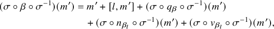 $$ \begin{align*} (\sigma\circ \beta\circ \sigma^{-1})(m') &= m' + [l,m'] + (\sigma \circ q_{\beta} \circ \sigma^{-1})(m') \\ &\quad+ (\sigma \circ n_{\beta_{l}} \circ \sigma^{-1})(m') + (\sigma \circ v_{\beta_{l}} \circ \sigma^{-1})(m') , \end{align*} $$
so $\gamma := \sigma \circ \beta \circ \sigma ^{-1}$
is again an l-exponential automorphism of
$\gamma := \sigma \circ \beta \circ \sigma ^{-1}$
is again an l-exponential automorphism of $L \otimes k'$
, with corresponding maps
$L \otimes k'$
, with corresponding maps $q_{\gamma }=\sigma \circ q_{\beta }\circ \sigma ^{-1}$
,
$q_{\gamma }=\sigma \circ q_{\beta }\circ \sigma ^{-1}$
, $n_{\gamma }=\sigma \circ n_{\beta }\circ \sigma ^{-1}$
and
$n_{\gamma }=\sigma \circ n_{\beta }\circ \sigma ^{-1}$
and $v_{\gamma }=\sigma \circ v_{\beta }\circ \sigma ^{-1}$
. Hence, Theorem 3.13(v) implies that there exists
$v_{\gamma }=\sigma \circ v_{\beta }\circ \sigma ^{-1}$
. Hence, Theorem 3.13(v) implies that there exists $\mu \in k'$
such that
$\mu \in k'$
such that $\gamma =\exp (\mu y)\beta $
, and by Remark 3.14 again, we have
$\gamma =\exp (\mu y)\beta $
, and by Remark 3.14 again, we have $q_\gamma = q_\beta + \operatorname {\mathrm {ad}}_{\mu y}$
. In particular,
$q_\gamma = q_\beta + \operatorname {\mathrm {ad}}_{\mu y}$
. In particular,
 $$ \begin{align*} b_1 \otimes \lambda_1^\sigma + \dots + b_n \otimes \lambda_n^\sigma &= q_{\gamma}(x) = [y,x] \otimes \mu +q_{\beta}(x) \\ &= [y,x] \otimes \mu + b_1 \otimes \lambda_1 + \dots + b_m \otimes \lambda_n. \end{align*} $$
Since $b_1,\dots , b_n$
and
$b_1,\dots , b_n$
and $[x,y]$
are linearly independent by construction, this implies
$[x,y]$
are linearly independent by construction, this implies $\mu =0$
, and thus,
$\mu =0$
, and thus, $\gamma = \beta $
. Since
$\gamma = \beta $
. Since $\sigma \in \operatorname {\mathrm {Gal}}(k'/k)$
was arbitrary, we get
$\sigma \in \operatorname {\mathrm {Gal}}(k'/k)$
was arbitrary, we get $\beta =\sigma \circ \beta \circ \sigma ^{-1}$
for all
$\beta =\sigma \circ \beta \circ \sigma ^{-1}$
for all $\sigma \in \operatorname {\mathrm {Gal}}(k'/k)$
, and therefore,
$\sigma \in \operatorname {\mathrm {Gal}}(k'/k)$
, and therefore,
 $$\begin{align*}q_{\beta}=\sigma\circ q_{\beta}\circ \sigma^{-1}, \quad n_{\beta}=\sigma\circ n_{\beta}\circ \sigma^{-1}, \quad v_{\beta}=\sigma\circ v_{\beta}\circ \sigma^{-1}, \end{align*}$$
for all $\sigma \in \operatorname {\mathrm {Gal}}(k'/k)$
. Since
$\sigma \in \operatorname {\mathrm {Gal}}(k'/k)$
. Since $k'/k$
is a Galois extension and thus
$k'/k$
is a Galois extension and thus $\operatorname {\mathrm {Fix}}(\operatorname {\mathrm {Gal}}(k'/k))=k$
, this implies that the maps
$\operatorname {\mathrm {Fix}}(\operatorname {\mathrm {Gal}}(k'/k))=k$
, this implies that the maps $q_\beta $
,
$q_\beta $
, $n_\beta $
and
$n_\beta $
and $v_\beta $
stabilize L, proving that the restriction of
$v_\beta $
stabilize L, proving that the restriction of $\beta $
to L is an automorphism of L. Since
$\beta $
to L is an automorphism of L. Since $\beta $
is an l-exponential automorphism, we are done.
$\beta $
is an l-exponential automorphism, we are done.
Remark 3.17. Under the assumptions of Theorem 3.16, many of the conclusions of Theorem 3.13 now remain valid, simply by extending the scalars to $k'$
. In particular, we are allowed to use Theorem 3.13(v) and (vii) to (ix) in this more general setting. (However, notice that Theorem 3.13(iv) and (vi) do not necessarily make sense over k because
$k'$
. In particular, we are allowed to use Theorem 3.13(v) and (vii) to (ix) in this more general setting. (However, notice that Theorem 3.13(iv) and (vi) do not necessarily make sense over k because $E \cap L_1$
might be empty.)
$E \cap L_1$
might be empty.)
Assumption 3.18. For the rest of this section, we assume that L is a simple Lie algebra over k with extremal elements x and y with $g(x,y)=1$
and that
$g(x,y)=1$
and that $k'/k$
is a Galois extension such that
$k'/k$
is a Galois extension such that $L\otimes k'$
is a simple Lie algebra generated by its pure extremal elements, with
$L\otimes k'$
is a simple Lie algebra generated by its pure extremal elements, with $\mathcal F(L\otimes k')\neq \emptyset $
and
$\mathcal F(L\otimes k')\neq \emptyset $
and $|k'|\geq 3$
.
$|k'|\geq 3$
.
In the next two lemmas, we determine how l-exponential automorphisms commute, extending Theorem 3.13(i).
Lemma 3.19. Let $l,l' \in L_1$
and let
$l,l' \in L_1$
and let $\alpha $
and
$\alpha $
and $\beta $
be an l-exponential and
$\beta $
be an l-exponential and $l'$
-exponential automorphism of L, respectively. Then
$l'$
-exponential automorphism of L, respectively. Then $\alpha \beta = \exp ([l,l'])\beta \alpha $
.
$\alpha \beta = \exp ([l,l'])\beta \alpha $
.
Proof. Notice that by Theorem 3.13(viii), both $\alpha \beta $
and
$\alpha \beta $
and $\exp ([l,l'])\beta \alpha $
are
$\exp ([l,l'])\beta \alpha $
are $(l+l')$
-exponential automorphisms. By the uniqueness statement of Remark 3.14, it remains to show that
$(l+l')$
-exponential automorphisms. By the uniqueness statement of Remark 3.14, it remains to show that $q_{\alpha \beta }(x) = q_{\exp ([l,l'])\beta \alpha }(x)$
. By Remark 3.14(ii), we have
$q_{\alpha \beta }(x) = q_{\exp ([l,l'])\beta \alpha }(x)$
. By Remark 3.14(ii), we have
 $$\begin{align*}q_{\alpha\beta}(x) = q_\alpha(x) + [l, [l',x]] + q_\beta(x) , \end{align*}$$
and by Remark 3.14(i), we have
 $$\begin{align*}q_{\exp([l,l'])\beta\alpha}(x) = q_\beta(x) + [l', [l,x]] + q_\alpha(x) + [[l,l'], x] , \end{align*}$$
so by the Jacobi identity, these expressions are indeed equal.
If $\operatorname {\mathrm {char}}(k)\neq 2$
, we can be more precise.
$\operatorname {\mathrm {char}}(k)\neq 2$
, we can be more precise.
Lemma 3.20. Assume $\operatorname {\mathrm {char}}(k)\neq 2$
and let
$\operatorname {\mathrm {char}}(k)\neq 2$
and let $l,l' \in L_1$
. Then
$l,l' \in L_1$
. Then
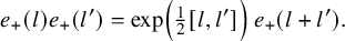 $$\begin{align*}e_+(l) e_+(l') = \exp\left(\tfrac{1}{2} [l,l']\right) \, e_+(l+l') .\end{align*}$$
Proof. Let $\alpha := e_+(l)$
,
$\alpha := e_+(l)$
, $\beta := e_+(l')$
,
$\beta := e_+(l')$
, $\gamma := e_+(l+l')$
and
$\gamma := e_+(l+l')$
and $z := \tfrac {1}{2} [l,l']$
. Exactly as in the proof of Lemma 3.19, we only have to show that
$z := \tfrac {1}{2} [l,l']$
. Exactly as in the proof of Lemma 3.19, we only have to show that $q_{\alpha \beta }(x) = q_{\exp (z) \gamma }(x)$
. Using Remark 3.14, we get
$q_{\alpha \beta }(x) = q_{\exp (z) \gamma }(x)$
. Using Remark 3.14, we get
 $$\begin{align*}q_{\alpha\beta}(x) = q_\alpha(x) + q_\beta(x) + [l, [l',x]] = \tfrac{1}{2}[l, [l, x]] + \tfrac{1}{2}[l', [l', x]] + [l, [l', x]] , \end{align*}$$
and
 $$\begin{align*}q_{\exp(z) \gamma}(x) = q_\gamma(x) + \tfrac{1}{2} [[l,l'], x] = \tfrac{1}{2}[l+l', [l+l', x]] + \tfrac{1}{2}[[l,l'], x] , \end{align*}$$
and again, the equality of these two expressions follows from the Jacobi identity.
If $\operatorname {\mathrm {char}}(k)\neq 2,3$
, we now get an explicit description of the maps
$\operatorname {\mathrm {char}}(k)\neq 2,3$
, we now get an explicit description of the maps $n_{e_+(l)}$
and
$n_{e_+(l)}$
and $v_{e_+(l)}$
. In particular, we recover in this case (and under our running Assumption 3.18) the fact that the Lie algebra is algebraic with respect to the given
$v_{e_+(l)}$
. In particular, we recover in this case (and under our running Assumption 3.18) the fact that the Lie algebra is algebraic with respect to the given $5$
-grading, as defined in Definition 1.10.
$5$
-grading, as defined in Definition 1.10.
Corollary 3.21. Assume that $\operatorname {\mathrm {char}}(k) \neq 2$
. Let
$\operatorname {\mathrm {char}}(k) \neq 2$
. Let $l \in L_1$
and let
$l \in L_1$
and let $\alpha := e_+(l)$
. Then
$\alpha := e_+(l)$
. Then
 $$\begin{align*}6 n_\alpha(m) = [l,[l,[l,m]]] \quad \text{and} \quad 24 v_\alpha(m) = [l,[l,[l,[l,m]]]] \end{align*}$$
for all $m \in L$
.
$m \in L$
.
Proof. Let $\beta := \alpha _{2}$
be as in Theorem 3.13(vii) and let
$\beta := \alpha _{2}$
be as in Theorem 3.13(vii) and let $\gamma := e_+(2l)$
as in Theorem 3.13(ix). Then
$\gamma := e_+(2l)$
as in Theorem 3.13(ix). Then $q_\beta = 2^2 q_\alpha $
while
$q_\beta = 2^2 q_\alpha $
while $q_\gamma (m) = \tfrac {1}{2}[2l, [2l, m]] = 4 q_\alpha (m)$
for all
$q_\gamma (m) = \tfrac {1}{2}[2l, [2l, m]] = 4 q_\alpha (m)$
for all $m \in L$
, so by the uniqueness part of Theorem 3.13(ix), we have
$m \in L$
, so by the uniqueness part of Theorem 3.13(ix), we have $\beta = \gamma $
. However, we have
$\beta = \gamma $
. However, we have $e_+(2l) = e_+(l + l) = e_+(l)^2$
by Lemma 3.20, so
$e_+(2l) = e_+(l + l) = e_+(l)^2$
by Lemma 3.20, so $\alpha _2 = \alpha ^2$
.
$\alpha _2 = \alpha ^2$
.
By Theorem 3.13(vii), we have $n_{\alpha _2} = 8 n_\alpha $
, while by Remark 3.14(ii), we have
$n_{\alpha _2} = 8 n_\alpha $
, while by Remark 3.14(ii), we have
 $$\begin{align*}n_{\alpha^2}(m) = 2 n_\alpha(m) + q_\alpha([l,m]) + [l, q_\alpha(m)] \end{align*}$$
for all $m \in L$
. Since
$m \in L$
. Since $q_\alpha (m) = \tfrac {1}{2}[l, [l, m]]$
, we conclude that
$q_\alpha (m) = \tfrac {1}{2}[l, [l, m]]$
, we conclude that $6 n_\alpha (m) = [l, [l, [l, m]]]$
for all
$6 n_\alpha (m) = [l, [l, [l, m]]]$
for all $m \in L$
.
$m \in L$
.
Similarly, we let $\delta := e_+(-l) e_+(l)$
, and we use the fact that
$\delta := e_+(-l) e_+(l)$
, and we use the fact that $\alpha _{-1} = \alpha ^{-1}$
. On the one hand,
$\alpha _{-1} = \alpha ^{-1}$
. On the one hand, $\delta = \operatorname {\mathrm {id}}$
, so
$\delta = \operatorname {\mathrm {id}}$
, so $v_\delta = 0$
, while on the other hand, by Remark 3.14(ii) again,
$v_\delta = 0$
, while on the other hand, by Remark 3.14(ii) again,
 $$\begin{align*}v_{\delta}(m) = 2 v_\alpha(m) - n_\alpha([l,m]) + q_\alpha(q_\alpha(m)) - [l, n_\alpha(m)] \end{align*}$$
for all $m \in L$
. Multiplying by
$m \in L$
. Multiplying by $12$
, we get
$12$
, we get $24 v_\alpha (m) = [l,[l,[l,[l,m]]]]$
, as required.
$24 v_\alpha (m) = [l,[l,[l,[l,m]]]]$
, as required.
Our final result of this section shows that $E_+(x,y)$
acts sharply transitively on the set of all extremal points with nonzero
$E_+(x,y)$
acts sharply transitively on the set of all extremal points with nonzero $L_{-2}$
-component.
$L_{-2}$
-component.
Proposition 3.22. Let L be a simple Lie algebra. Assume that for some Galois extension $k'/k$
with
$k'/k$
with $k'\neq \mathbb F_2$
,
$k'\neq \mathbb F_2$
, $L_{k'} := L \otimes _k k'$
is a simple Lie algebra generated by its pure extremal elements and has
$L_{k'} := L \otimes _k k'$
is a simple Lie algebra generated by its pure extremal elements and has $\mathcal {F}(L_{k'})\neq \emptyset $
.
$\mathcal {F}(L_{k'})\neq \emptyset $
.
Consider a hyperbolic pair $x,y\in E$
with
$x,y\in E$
with $g(x,y)=1$
and let
$g(x,y)=1$
and let $L=L_{-2}\oplus L_{-1}\oplus L_0\oplus L_1\oplus L_2$
be the associated
$L=L_{-2}\oplus L_{-1}\oplus L_0\oplus L_1\oplus L_2$
be the associated $5$
-grading.
$5$
-grading.
Then every extremal element with $L_{-2}$
-component equal to x can be written as
$L_{-2}$
-component equal to x can be written as $\varphi (x)$
for a unique
$\varphi (x)$
for a unique $\varphi \in E_+(x,y)$
.
$\varphi \in E_+(x,y)$
.
Proof. Let e be an extremal element with $L_{-2}$
-component equal to x. We first show the existence of an automorphism
$L_{-2}$
-component equal to x. We first show the existence of an automorphism $\varphi \in E_+(x,y)$
with
$\varphi \in E_+(x,y)$
with $\varphi (x) = e$
.
$\varphi (x) = e$
.
Let $e_{-1}$
be the
$e_{-1}$
be the $L_{-1}$
-component of e. By Proposition 2.4(iii), there is a (unique)
$L_{-1}$
-component of e. By Proposition 2.4(iii), there is a (unique) $a \in L_1$
such that
$a \in L_1$
such that $[a,x] = e_{-1}$
. By Theorem 3.16, there exists an a-exponential automorphism
$[a,x] = e_{-1}$
. By Theorem 3.16, there exists an a-exponential automorphism $\alpha \in E_+(x,y)$
. Then
$\alpha \in E_+(x,y)$
. Then $\alpha ^{-1}(e) = x + l_0 + l_1 + l_2$
, with
$\alpha ^{-1}(e) = x + l_0 + l_1 + l_2$
, with $l_i\in L_i$
. By Lemma 3.10, there exists
$l_i\in L_i$
. By Lemma 3.10, there exists $\lambda \in k$
such that
$\lambda \in k$
such that $\exp (\lambda y)(x) = \alpha ^{-1}(e)$
. This shows that
$\exp (\lambda y)(x) = \alpha ^{-1}(e)$
. This shows that $\varphi := \alpha \exp (\lambda y) \in E_+(x,y)$
maps x to e, as required.
$\varphi := \alpha \exp (\lambda y) \in E_+(x,y)$
maps x to e, as required.
To show uniqueness, assume that also $\varphi '\in E_+(x,y)$
satisfies
$\varphi '\in E_+(x,y)$
satisfies $\varphi '(x)=e=\varphi (x)$
. In particular,
$\varphi '(x)=e=\varphi (x)$
. In particular, $\varphi $
and
$\varphi $
and $\varphi '$
are l-exponential automorphisms for the same
$\varphi '$
are l-exponential automorphisms for the same $l \in L_1$
. This implies that also
$l \in L_1$
. This implies that also $\varphi (m) = m + [l,m] = \varphi '(m)$
for all
$\varphi (m) = m + [l,m] = \varphi '(m)$
for all $m\in L_{1}$
. Since L is generated by
$m\in L_{1}$
. Since L is generated by $\{ x \} \cup L_1$
, we conclude that
$\{ x \} \cup L_1$
, we conclude that $\varphi = \varphi '$
.
$\varphi = \varphi '$
.
Remark 3.23. Note that we did not make any assumptions on the dimension of the Lie algebra L in this section. In particular, the results also hold for infinite-dimensional Lie algebras.
4 Extremal geometry with lines – recovering a cubic norm structure
In this section, we prove that if L is a simple Lie algebra over a field k with $|k| \geq 4$
, which is generated by its pure extremal elements and such that its extremal geometry contains lines, then
$|k| \geq 4$
, which is generated by its pure extremal elements and such that its extremal geometry contains lines, then $L_1$
can be decomposed as
$L_1$
can be decomposed as $k\oplus J\oplus J' \oplus k$
, for a certain ‘twin cubic norm structure’
$k\oplus J\oplus J' \oplus k$
, for a certain ‘twin cubic norm structure’ $(J, J')$
. If the norm of this twin cubic norm structure is not the zero map, then
$(J, J')$
. If the norm of this twin cubic norm structure is not the zero map, then $J' \cong J$
and J gets the structure of a genuine cubic norm structure (depending on the choice of a ‘base point’). At the end of this section, we also sketch how the Lie algebra L can be completely reconstructed from this cubic norm structure.
$J' \cong J$
and J gets the structure of a genuine cubic norm structure (depending on the choice of a ‘base point’). At the end of this section, we also sketch how the Lie algebra L can be completely reconstructed from this cubic norm structure.
Assumption 4.1. Throughout the whole section, we assume that L is a simple Lie algebra defined over a field k with $|k| \geq 4$
, such that L is generated by its pure extremal elements and such that the extremal geometry contains lines.
$|k| \geq 4$
, such that L is generated by its pure extremal elements and such that the extremal geometry contains lines.
We fix a pair of extremal elements $x,y \in E$
with
$x,y \in E$
with $g(x,y)=1$
, and we consider the corresponding
$g(x,y)=1$
, and we consider the corresponding $5$
-grading
$5$
-grading $L=L_{-2}\oplus L_{-1}\oplus L_0\oplus L_1\oplus L_2$
as in Proposition 2.4.
$L=L_{-2}\oplus L_{-1}\oplus L_0\oplus L_1\oplus L_2$
as in Proposition 2.4.
Notation 4.2. Since the extremal geometry contains lines, Proposition 2.16 implies that there exist extremal elements c and d contained in $L_{-1}$
such that
$L_{-1}$
such that $[c,d]=x$
. Set
$[c,d]=x$
. Set $p := [y,c]$
and
$p := [y,c]$
and $q := -[y,d]$
, so
$q := -[y,d]$
, so $p,q \in L_1$
. By Proposition 2.16 again, we see that
$p,q \in L_1$
. By Proposition 2.16 again, we see that $[x,y]=[c+d,p+q] = [c,q] + [d,p]$
. (Notice that
$[x,y]=[c+d,p+q] = [c,q] + [d,p]$
. (Notice that $[c,p]=0$
and
$[c,p]=0$
and $[d,q]=0$
.) Observe that both
$[d,q]=0$
.) Observe that both $(c,d)$
and
$(c,d)$
and $(p,q)$
are special pairs, with
$(p,q)$
are special pairs, with $[c,d] = x$
and
$[c,d] = x$
and $[q,p] = y$
.
$[q,p] = y$
.
We start with the following observation, needed to obtain a second grading on the Lie algebra which we will use often in this section.
Lemma 4.3. We have $g(p, d) = 1$
and
$g(p, d) = 1$
and $g(q, c) = 1$
.
$g(q, c) = 1$
.
Proof. We have $g(p, d) = g([y, c], d) = g(y, [c, d]) = g(y,x) = 1$
and
$g(p, d) = g([y, c], d) = g(y, [c, d]) = g(y,x) = 1$
and $g(q, c) = g(-[y, d], c) = -g(y, [d, c]) = g(y, x) = 1$
.
$g(q, c) = g(-[y, d], c) = -g(y, [d, c]) = g(y, x) = 1$
.
We are now ready to define a subspace J which will turn out to have the structure of a cubic norm structure. Using the grading related to $(c,q)\in E_2$
, we are able to describe a decomposition of
$(c,q)\in E_2$
, we are able to describe a decomposition of $L_{-1}$
into
$L_{-1}$
into $4$
parts.
$4$
parts.
Notation 4.4. We denote the $5$
-grading of L obtained by considering the pair
$5$
-grading of L obtained by considering the pair $(c,q)\in E_2$
in Proposition 2.4 by
$(c,q)\in E_2$
in Proposition 2.4 by
 $$ \begin{align} L=L^{\prime}_{-2}\oplus L^{\prime}_{-1}\oplus L^{\prime}_{0}\oplus L^{\prime}_{1}\oplus L^{\prime}_{2}, \end{align} $$
where $L^{\prime }_{-2}=\langle c\rangle $
and
$L^{\prime }_{-2}=\langle c\rangle $
and $L^{\prime }_2=\langle q\rangle $
. We will occasionally also need a third grading arising from the hyperbolic pair
$L^{\prime }_2=\langle q\rangle $
. We will occasionally also need a third grading arising from the hyperbolic pair $(d,p) \in E_2$
, denoted by
$(d,p) \in E_2$
, denoted by
 $$ \begin{align} L=L^{\prime\prime}_{-2}\oplus L^{\prime\prime}_{-1}\oplus L^{\prime\prime}_{0}\oplus L^{\prime\prime}_{1}\oplus L^{\prime\prime}_{2}, \end{align} $$
where $L^{\prime \prime }_{-2}=\langle d\rangle $
and
$L^{\prime \prime }_{-2}=\langle d\rangle $
and $L^{\prime \prime }_2=\langle p\rangle $
.
$L^{\prime \prime }_2=\langle p\rangle $
.
We set
 $$ \begin{align*} J = L_{-1}\cap L^{\prime}_{-1},\ J'=L_{-1}\cap L^{\prime}_0. \end{align*} $$
Lemma 4.5. We have
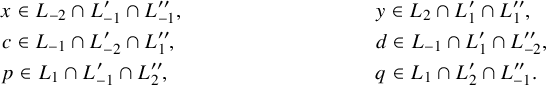 $$\begin{align*} &x \in L_{-2} \cap L^{\prime}_{-1} \cap L^{\prime\prime}_{-1}, \qquad &&y \in L_2 \cap L^{\prime}_{1} \cap L^{\prime\prime}_{1}, \\ &c \in L_{-1} \cap L^{\prime}_{-2} \cap L^{\prime\prime}_{1}, \qquad &&d \in L_{-1} \cap L^{\prime}_{1} \cap L^{\prime\prime}_{-2}, \\ &p \in L_1 \cap L^{\prime}_{-1} \cap L^{\prime\prime}_{2}, \qquad &&q \in L_1 \cap L^{\prime}_{2} \cap L^{\prime\prime}_{-1}. \end{align*}$$
Proof. By our setup in Notation 4.2, the extremal points $\langle x\rangle ,\langle c \rangle ,\langle p \rangle ,\langle y \rangle ,\langle q \rangle ,\langle d \rangle ,\langle x \rangle $
form an ordinary hexagon in the extremal geometry, where all pairs at distance two are special. Now all containments follow either directly from the grading (for the
$\langle x\rangle ,\langle c \rangle ,\langle p \rangle ,\langle y \rangle ,\langle q \rangle ,\langle d \rangle ,\langle x \rangle $
form an ordinary hexagon in the extremal geometry, where all pairs at distance two are special. Now all containments follow either directly from the grading (for the $-2$
- and
$-2$
- and $2$
-components), or they follow from Lemma 2.14 (for the
$2$
-components), or they follow from Lemma 2.14 (for the $-1$
- and
$-1$
- and $1$
-components).
$1$
-components).
We now obtain a decomposition of $L_{-1}$
into
$L_{-1}$
into $4$
parts, by intersecting with the
$4$
parts, by intersecting with the $L^{\prime }_i$
-grading (17) arising from the hyperbolic pair
$L^{\prime }_i$
-grading (17) arising from the hyperbolic pair $(c,q)$
.
$(c,q)$
.
Proposition 4.6. We have a decomposition
 $$ \begin{align*} L_{-1}=\langle c\rangle \oplus J\oplus J'\oplus \langle d\rangle. \end{align*} $$
Moreover, $L_{-1}\cap L^{\prime }_1=\langle d\rangle $
.
$L_{-1}\cap L^{\prime }_1=\langle d\rangle $
.
Proof. Since $c \in L_{-1}$
, we have
$c \in L_{-1}$
, we have $g_{c}(L_{-1})=0$
by Lemma 2.15. However, we also have
$g_{c}(L_{-1})=0$
by Lemma 2.15. However, we also have $c\in L^{\prime }_{-2}$
, so we get
$c\in L^{\prime }_{-2}$
, so we get $L_{-1} \leq L^{\prime }_{\leq 1}$
by Proposition 2.4(iv).
$L_{-1} \leq L^{\prime }_{\leq 1}$
by Proposition 2.4(iv).
Now let $l\in L_{-1}$
be arbitrary, and write
$l\in L_{-1}$
be arbitrary, and write $l = l^{\prime }_{-2}+l^{\prime }_{-1}+l^{\prime }_0+l^{\prime }_1$
with each
$l = l^{\prime }_{-2}+l^{\prime }_{-1}+l^{\prime }_0+l^{\prime }_1$
with each $l^{\prime }_i \in L^{\prime }_i$
. Since
$l^{\prime }_i \in L^{\prime }_i$
. Since $L^{\prime }_{-2}=\langle c\rangle \leq L_{-1}$
, we may assume
$L^{\prime }_{-2}=\langle c\rangle \leq L_{-1}$
, we may assume $l^{\prime }_{-2}=0$
.
$l^{\prime }_{-2}=0$
.
Now observe that by Proposition 2.4(ii), $[[c,q], l] = -l^{\prime }_{-1} + l^{\prime }_1$
. However,
$[[c,q], l] = -l^{\prime }_{-1} + l^{\prime }_1$
. However, $[c,q]\in L_0$
, so
$[c,q]\in L_0$
, so $[[c,q],l]\in L_{-1}$
, and we deduce that
$[[c,q],l]\in L_{-1}$
, and we deduce that
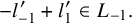 $$ \begin{align} -l^{\prime}_{-1} + l^{\prime}_1 \in L_{-1}. \end{align} $$
Next, let $\lambda \in k$
be any nonzero scalar and consider the automorphism
$\lambda \in k$
be any nonzero scalar and consider the automorphism $\varphi _\lambda \in \operatorname {\mathrm {Aut}}(L)$
defined in Lemma 2.10, but with respect to the
$\varphi _\lambda \in \operatorname {\mathrm {Aut}}(L)$
defined in Lemma 2.10, but with respect to the $5$
-grading (17). Since
$5$
-grading (17). Since $x\in L^{\prime }_{-1}$
and
$x\in L^{\prime }_{-1}$
and $y\in L^{\prime }_1$
, we have
$y\in L^{\prime }_1$
, we have $\varphi _\lambda (x)=\lambda ^{-1} x$
and
$\varphi _\lambda (x)=\lambda ^{-1} x$
and $\varphi _\lambda (y)=\lambda y$
. Then Lemma 2.12 implies
$\varphi _\lambda (y)=\lambda y$
. Then Lemma 2.12 implies $\varphi _\lambda (L_{-1})=L_{-1}$
. In particular,
$\varphi _\lambda (L_{-1})=L_{-1}$
. In particular, $\varphi _\lambda (l)=\lambda ^{-1}l^{\prime }_{-1}+l^{\prime }_0+\lambda l^{\prime }_1$
is contained in
$\varphi _\lambda (l)=\lambda ^{-1}l^{\prime }_{-1}+l^{\prime }_0+\lambda l^{\prime }_1$
is contained in $L_{-1}$
, so subtracting
$L_{-1}$
, so subtracting $l \in L_{-1}$
, we see that
$l \in L_{-1}$
, we see that
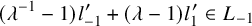 $$\begin{align*}(\lambda^{-1}-1)l^{\prime}_{-1}+(\lambda-1)l^{\prime}_1\in L_{-1} \end{align*}$$
for all nonzero $\lambda \in k$
. Combining this with (19), we get
$\lambda \in k$
. Combining this with (19), we get $(\lambda ^{-1} + \lambda - 2)l^{\prime }_{-1}\in L_{-1}$
for all nonzero
$(\lambda ^{-1} + \lambda - 2)l^{\prime }_{-1}\in L_{-1}$
for all nonzero $\lambda \in k$
. If
$\lambda \in k$
. If $\operatorname {\mathrm {char}} (k)\neq 2$
, we can take
$\operatorname {\mathrm {char}} (k)\neq 2$
, we can take $\lambda =-1$
to get
$\lambda =-1$
to get $l^{\prime }_{-1}\in L_{-1}$
, while if
$l^{\prime }_{-1}\in L_{-1}$
, while if $\operatorname {\mathrm {char}}(k)=2$
, then
$\operatorname {\mathrm {char}}(k)=2$
, then $|k|>2$
implies that we can find
$|k|>2$
implies that we can find $\lambda $
such that
$\lambda $
such that $\lambda +\lambda ^{-1}\neq 0$
. In both cases, we conclude that
$\lambda +\lambda ^{-1}\neq 0$
. In both cases, we conclude that $l^{\prime }_{-1}\in L_{-1}$
, and then by (19) again, also
$l^{\prime }_{-1}\in L_{-1}$
, and then by (19) again, also $l^{\prime }_1 \in L_{-1}$
. Since
$l^{\prime }_1 \in L_{-1}$
. Since $l = l^{\prime }_{-1}+l^{\prime }_0+l^{\prime }_1$
, also
$l = l^{\prime }_{-1}+l^{\prime }_0+l^{\prime }_1$
, also $l^{\prime }_0 \in L_{-1}$
. Hence,
$l^{\prime }_0 \in L_{-1}$
. Hence,
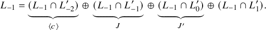 $$\begin{align*}L_{-1} = \underbrace{(L_{-1} \cap L^{\prime}_{-2})}_{\langle c \rangle} \, \oplus \, \underbrace{(L_{-1} \cap L^{\prime}_{-1})}_{J} \, \oplus \, \underbrace{(L_{-1} \cap L^{\prime}_0)}_{J'} \, \oplus \; {(L_{-1} \cap L^{\prime}_1)}. \end{align*}$$
Finally, let $l^{\prime }_1\in L_{-1} \cap L^{\prime }_1$
be arbitrary. By Proposition 2.4(iii), we get
$l^{\prime }_1\in L_{-1} \cap L^{\prime }_1$
be arbitrary. By Proposition 2.4(iii), we get $[q,[c,l^{\prime }_1]] = -l^{\prime }_1$
. Since
$[q,[c,l^{\prime }_1]] = -l^{\prime }_1$
. Since $[c,l^{\prime }_1]\in L_{-2} = \langle x\rangle $
, this implies that
$[c,l^{\prime }_1]\in L_{-2} = \langle x\rangle $
, this implies that $l^{\prime }_1$
is a multiple of
$l^{\prime }_1$
is a multiple of $[q,x]=-d$
. Hence,
$[q,x]=-d$
. Hence, $L_{-1} \cap L^{\prime }_1 = \langle d\rangle $
.
$L_{-1} \cap L^{\prime }_1 = \langle d\rangle $
.
Using this decomposition, we obtain some more information on the Lie bracket.
Corollary 4.7. We have a decomposition
 $$ \begin{align*} L_1=\langle p\rangle \oplus [y,J]\oplus [y,J']\oplus \langle q\rangle. \end{align*} $$
Moreover,
 $$ \begin{align} &\langle p\rangle =L_1\cap L^{\prime}_{-1},&& [y,J]=L_1\cap L^{\prime}_{0}, && [y,J']=L_1\cap L^{\prime}_1; \end{align} $$
 $$ \begin{align} &[J,J]=0, && [J,c]=[J,d]=0, &&[J,p]=0; \end{align} $$
 $$ \begin{align} &[J',J']=0, && [J',c]=[J',d]=0, &&[J',q]=0; \end{align} $$
 $$ \begin{align} &[J,[J,q]]\leq J', && [J',[J',p]]\leq J. \end{align} $$
Proof. By Proposition 2.4(iii), the map $\operatorname {\mathrm {ad}}_y \colon L_{-1} \to L_1$
is an isomorphism of vector spaces, so the decomposition is clear. The identities (20) now follow from this new decomposition.
$\operatorname {\mathrm {ad}}_y \colon L_{-1} \to L_1$
is an isomorphism of vector spaces, so the decomposition is clear. The identities (20) now follow from this new decomposition.
Next, by combining both gradings, we have
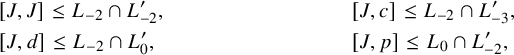 $$\begin{align*} & [J,J] \leq L_{-2} \cap L^{\prime}_{-2}, \quad && [J,c] \leq L_{-2} \cap L^{\prime}_{-3}, \\ & [J,d] \leq L_{-2} \cap L^{\prime}_{0}, \quad && [J,p] \leq L_0 \cap L^{\prime}_{-2}, \end{align*}$$
but since $L_{-2} = \langle x \rangle \leq L^{\prime }_{-1}$
and
$L_{-2} = \langle x \rangle \leq L^{\prime }_{-1}$
and $L^{\prime }_{-2} = \langle c \rangle \leq L_{-1}$
, all four intersections are trivial, proving (21). The proof of (22) is similar.
$L^{\prime }_{-2} = \langle c \rangle \leq L_{-1}$
, all four intersections are trivial, proving (21). The proof of (22) is similar.
Finally, $[J, [J, q]] \leq L_{-1-1+1} \cap L^{\prime }_{-1-1+2} = L_{-1} \cap L^{\prime }_{0} = J'$
, and similarly, we have
$[J, [J, q]] \leq L_{-1-1+1} \cap L^{\prime }_{-1-1+2} = L_{-1} \cap L^{\prime }_{0} = J'$
, and similarly, we have $[J', [J', p]] \leq L_{-1} \cap L^{\prime }_{-1} = J$
, showing (23).
$[J', [J', p]] \leq L_{-1} \cap L^{\prime }_{-1} = J$
, showing (23).
Lemma 4.8. We have
 $$ \begin{align} J &=\{ l\in L_{-1} \mid [c,l] = [d,l] = [p,l] = 0 \}, \end{align} $$
 $$ \begin{align} J' &=\{ l\in L_{-1} \mid [c,l] = [d,l] = [q,l] = 0 \}. \end{align} $$
Proof. By (21), it is clear that J is contained in the set on the right-hand side of (24).
Conversely, let $l\in L_{-1}$
such that
$l\in L_{-1}$
such that $[c,l] = [d,l] = [p,l] = 0$
and use Proposition 4.6 to write
$[c,l] = [d,l] = [p,l] = 0$
and use Proposition 4.6 to write $l = \lambda c + j + j' + \mu d$
, with
$l = \lambda c + j + j' + \mu d$
, with $\lambda ,\mu \in k$
,
$\lambda ,\mu \in k$
, $j \in J$
and
$j \in J$
and $j' \in J'$
. Since
$j' \in J'$
. Since $[c,d]\neq 0$
, it already follows from
$[c,d]\neq 0$
, it already follows from $[c,l] = 0$
that
$[c,l] = 0$
that $\mu = 0$
and from
$\mu = 0$
and from $[d,l] = 0$
that
$[d,l] = 0$
that $\lambda = 0$
, so we already have
$\lambda = 0$
, so we already have $l = j + j'$
, and it remains to show that
$l = j + j'$
, and it remains to show that $j' = 0$
.
$j' = 0$
.
Since $[p,l] = 0$
and
$[p,l] = 0$
and $[p,j] = 0$
, we have
$[p,j] = 0$
, we have $[p, j'] = 0$
. Recall from Notation 4.2 that
$[p, j'] = 0$
. Recall from Notation 4.2 that $[x,y] = [c,q] + [d,p]$
and
$[x,y] = [c,q] + [d,p]$
and $[d, j'] = 0$
. Since
$[d, j'] = 0$
. Since $j'\in L_{-1} \cap L^{\prime }_0$
, we can use Proposition 2.4(ii) twice to get
$j'\in L_{-1} \cap L^{\prime }_0$
, we can use Proposition 2.4(ii) twice to get
 $$\begin{align*}-j' = [[x,y],j'] = [[c,q],j'] + [[d,p],j'] = [d,[p,j']] = 0, \end{align*}$$
as claimed. The proof of (25) is completely similar.
The subspace $L_0$
also has a decomposition, but this time it is a decomposition into
$L_0$
also has a decomposition, but this time it is a decomposition into $3$
parts.
$3$
parts.
Proposition 4.9. We have a decomposition
 $$ \begin{align} L_0=(L_0\cap L^{\prime}_{-1})\oplus (L_0\cap L^{\prime}_0)\oplus (L_0\cap L^{\prime}_1). \end{align} $$
Moreover,
 $$ \begin{align} L_0\cap L^{\prime}_1 = [q,J] \quad \text{and} \quad L_0\cap L^{\prime}_{-1} = [p,J']. \end{align} $$
Proof. By Lemma 2.15 applied to $c\in L_{-1}$
, we get
$c\in L_{-1}$
, we get $g_{c}(L_0)=0$
. By Proposition 2.4(iv), this implies
$g_{c}(L_0)=0$
. By Proposition 2.4(iv), this implies $L_{0}\leq L^{\prime }_{-2}\oplus L^{\prime }_{-1}\oplus L^{\prime }_0\oplus L^{\prime }_1$
. Similarly,
$L_{0}\leq L^{\prime }_{-2}\oplus L^{\prime }_{-1}\oplus L^{\prime }_0\oplus L^{\prime }_1$
. Similarly, $g_q(L_0) = 0$
implies
$g_q(L_0) = 0$
implies $L_0\leq L^{\prime }_{-1}\oplus L^{\prime }_0\oplus L^{\prime }_1\oplus L^{\prime }_2$
. Hence,
$L_0\leq L^{\prime }_{-1}\oplus L^{\prime }_0\oplus L^{\prime }_1\oplus L^{\prime }_2$
. Hence, $L_0\leq L^{\prime }_{-1}\oplus L^{\prime }_0\oplus L^{\prime }_1$
.
$L_0\leq L^{\prime }_{-1}\oplus L^{\prime }_0\oplus L^{\prime }_1$
.
We can now apply the same technique as in the proof of Proposition 4.6. So let $l \in L_0$
be arbitrary and write
$l \in L_0$
be arbitrary and write $l = l^{\prime }_{-1} + l^{\prime }_0 + l^{\prime }_1$
with each
$l = l^{\prime }_{-1} + l^{\prime }_0 + l^{\prime }_1$
with each $l^{\prime }_i \in L^{\prime }_i$
. Again,
$l^{\prime }_i \in L^{\prime }_i$
. Again, $[[c,q],l] = - l^{\prime }_{-1} + l^{\prime }_1 \in L_0$
, and using the automorphisms
$[[c,q],l] = - l^{\prime }_{-1} + l^{\prime }_1 \in L_0$
, and using the automorphisms $\varphi _\lambda $
, we get
$\varphi _\lambda $
, we get $\lambda _{-1} l^{\prime }_{-1} + l^{\prime }_0 + \lambda l^{\prime }_1 \in L_0$
for all
$\lambda _{-1} l^{\prime }_{-1} + l^{\prime }_0 + \lambda l^{\prime }_1 \in L_0$
for all $\lambda \in k^\times $
, yielding
$\lambda \in k^\times $
, yielding $l^{\prime }_i \in L_0$
for all three values of i, exactly as in the proof of Proposition 4.6. This proves (26).
$l^{\prime }_i \in L_0$
for all three values of i, exactly as in the proof of Proposition 4.6. This proves (26).
To show (27), notice that the inclusions $[q, J] \leq L_0 \cap L^{\prime }_1$
and
$[q, J] \leq L_0 \cap L^{\prime }_1$
and $[p,J'] \leq L_0 \cap L^{\prime }_{-1}$
are clear from the gradings. Conversely, let
$[p,J'] \leq L_0 \cap L^{\prime }_{-1}$
are clear from the gradings. Conversely, let $l_0\in L_0\cap L^{\prime }_1$
be arbitrary and let
$l_0\in L_0\cap L^{\prime }_1$
be arbitrary and let $l := - [c, l_0]$
. Then
$l := - [c, l_0]$
. Then $l \in L_{-1} \cap L^{\prime }_{-1} = J$
. By Proposition 2.4(iii), we have
$l \in L_{-1} \cap L^{\prime }_{-1} = J$
. By Proposition 2.4(iii), we have $l_0 = [q,l]$
, so indeed,
$l_0 = [q,l]$
, so indeed, $l_0 \in [q, J]$
. Similarly, let
$l_0 \in [q, J]$
. Similarly, let $l_0 \in L_0 \cap L^{\prime }_{-1}$
be arbitrary and let
$l_0 \in L_0 \cap L^{\prime }_{-1}$
be arbitrary and let $l := -[d, l_0]$
. Then
$l := -[d, l_0]$
. Then $l \in L_{-1} \cap L^{\prime }_0 = J'$
. By Proposition 2.4(iii) again, we have
$l \in L_{-1} \cap L^{\prime }_0 = J'$
. By Proposition 2.4(iii) again, we have $l_0 = [p,l]$
, so indeed,
$l_0 = [p,l]$
, so indeed, $l_0 \in [p, J']$
.
$l_0 \in [p, J']$
.
In the next lemma, we deduce some connections between the two gradings (17) and (18).
Lemma 4.10. We have
 $$ \begin{align} &L_{-1}\cap L^{\prime\prime}_{-1}=J', && L_{-1}\cap L^{\prime\prime}_0=J, &&L_{-1}\cap L^{\prime\prime}_{1}=\langle c\rangle, \end{align} $$
 $$ \begin{align} &L_0\cap L^{\prime\prime}_{-1}=[q,J], &&L_0\cap L^{\prime\prime}_0=L_0\cap L^{\prime}_0, &&L_0\cap L^{\prime\prime}_{1}=[p,J']. \end{align} $$
Proof. Notice that in the setup in Notation 4.2, we can replace c with d, d with $-c$
, p with
$-c$
, p with $-q$
and q with p. In the resulting decompositions introduced in Notation 4.4, this interchanges the two gradings (17) and (18). If we subsequently set
$-q$
and q with p. In the resulting decompositions introduced in Notation 4.4, this interchanges the two gradings (17) and (18). If we subsequently set $K := L_{-1} \cap L^{\prime \prime }_{-1}$
and
$K := L_{-1} \cap L^{\prime \prime }_{-1}$
and $K' := L_{-1} \cap L^{\prime \prime }_0$
, then it follows from Lemma 4.8 that
$K' := L_{-1} \cap L^{\prime \prime }_0$
, then it follows from Lemma 4.8 that $K = J'$
and
$K = J'$
and $K' = J$
. By Proposition 4.6 applied on this new setup, we get
$K' = J$
. By Proposition 4.6 applied on this new setup, we get
 $$\begin{align*}L_{-1} = \langle d\rangle \oplus K \oplus K' \oplus \langle c\rangle \end{align*}$$
with $\langle c\rangle =L_{-1}\cap L^{\prime \prime }_{1}$
. This shows (28).
$\langle c\rangle =L_{-1}\cap L^{\prime \prime }_{1}$
. This shows (28).
By (27) applied on our new setup, we get $L_0\cap L^{\prime \prime }_1 = [p, J']$
and
$L_0\cap L^{\prime \prime }_1 = [p, J']$
and $L_0\cap L^{\prime \prime }_{-1}=[q,J]$
. Finally, consider
$L_0\cap L^{\prime \prime }_{-1}=[q,J]$
. Finally, consider $l\in L_0\cap L^{\prime \prime }_0$
. By Proposition 2.4(ii), we have
$l\in L_0\cap L^{\prime \prime }_0$
. By Proposition 2.4(ii), we have $[[x,y], l] = 0$
and
$[[x,y], l] = 0$
and $[[d,p], l] = 0$
. Recall from Notation 4.2 that
$[[d,p], l] = 0$
. Recall from Notation 4.2 that $[x,y] = [c,q] + [d,p]$
, so we get
$[x,y] = [c,q] + [d,p]$
, so we get
 $$\begin{align*}0 = [[x,y],l] = [[c,q],l]+[[d,p],l]=[[c,q],l].\end{align*}$$
Hence, l is contained in the $0$
-eigenspace of
$0$
-eigenspace of $\operatorname {\mathrm {ad}}_{[c,q]}$
, which is
$\operatorname {\mathrm {ad}}_{[c,q]}$
, which is $L^{\prime }_0$
by Proposition 2.4(ii) again. Hence,
$L^{\prime }_0$
by Proposition 2.4(ii) again. Hence, $L_0\cap L^{\prime \prime }_0\leq L_0\cap L^{\prime }_0$
, and
$L_0\cap L^{\prime \prime }_0\leq L_0\cap L^{\prime }_0$
, and $L_0\cap L^{\prime }_0\leq L_0\cap L^{\prime \prime }_0$
follows similarly. This shows (29).
$L_0\cap L^{\prime }_0\leq L_0\cap L^{\prime \prime }_0$
follows similarly. This shows (29).
We have summarized all the information about the intersections of the different gradings in Figure 1.
Now that we have a complete understanding of how the different gradings intersect, we are ready to invoke our results from Section 3. The next result on the uniqueness of certain extremal elements will play a key role in defining the maps involved in the cubic norm structure.
Proposition 4.11.
-
(i) For every
$a\in J$
, there is a unique extremal element of the form with
$$\begin{align*}a_{-2}+a_{-1}+[a,q]+q,\end{align*}$$
$a_{-2}\in L_{-2}$
and
$a_{-1}\in J'$
. This element is equal to
$\alpha (q)$
for a unique a-exponential automorphism
$\alpha \in E_-(x,y)$
.
-
(ii) For every
$b\in J'$
, there is a unique extremal element of the form with
$$\begin{align*}b_{-2}+b_{-1}+[b,p]+p,\end{align*}$$
$b_{-2}\in L_{-2}$
and
$b_{-1}\in J'$
. This element is equal to
$\beta (q)$
for a unique b-exponential automorphism
$\beta \in E_-(x,y)$
.


Proof. We show (i); the proof of (ii) is completely similar. By Theorem 3.13(iv), there exists an a-exponential automorphism $\alpha $
, so we have a corresponding extremal element
$\alpha $
, so we have a corresponding extremal element
 $$\begin{align*}\alpha(q)=a_{-2}+a_{-1}+[a,q]+q , \end{align*}$$
with $a_{-1}\in L_{-1}$
and
$a_{-1}\in L_{-1}$
and $a_{-2}\in L_{-2}$
. Notice that
$a_{-2}\in L_{-2}$
. Notice that $\alpha (d) = d + [a,d] = d$
because
$\alpha (d) = d + [a,d] = d$
because $[J,d] = 0$
by (21). By Proposition 2.4(iv), this implies that
$[J,d] = 0$
by (21). By Proposition 2.4(iv), this implies that $\alpha $
preserves the filtration
$\alpha $
preserves the filtration $L^{\prime \prime }_{\leq i}$
, so in particular,
$L^{\prime \prime }_{\leq i}$
, so in particular, $\alpha (q) \in L^{\prime \prime }_{\leq -1}$
. Hence,
$\alpha (q) \in L^{\prime \prime }_{\leq -1}$
. Hence, $a_{-1}\in L_{-1} \cap L^{\prime \prime }_{\leq -1} = \langle d\rangle \oplus J'$
(see Figure 1).
$a_{-1}\in L_{-1} \cap L^{\prime \prime }_{\leq -1} = \langle d\rangle \oplus J'$
(see Figure 1).
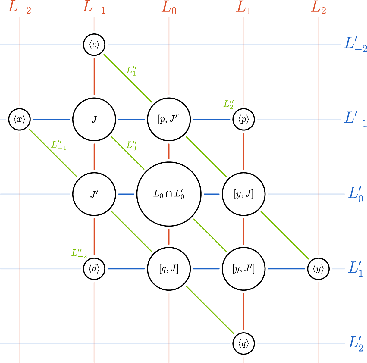
Figure 1 Intersecting gradings for cubic norm structures.
Now, since $[x,q]=[x,-[y,d]]=-[[x,y],d]=d$
, there is a (unique)
$[x,q]=[x,-[y,d]]=-[[x,y],d]=d$
, there is a (unique) $\lambda \in k$
such that
$\lambda \in k$
such that $\exp (\lambda x)(\alpha (q))$
has its
$\exp (\lambda x)(\alpha (q))$
has its $L_{-1}$
-component in
$L_{-1}$
-component in $J'$
. By replacing
$J'$
. By replacing $\alpha $
with
$\alpha $
with $\exp (\lambda x)\alpha $
, we find the required a-exponential automorphism and the required extremal element.
$\exp (\lambda x)\alpha $
, we find the required a-exponential automorphism and the required extremal element.
We now show uniqueness, so suppose that $e = b_{-2} + b_{-1} + [a,q] + q$
is an extremal element such that
$e = b_{-2} + b_{-1} + [a,q] + q$
is an extremal element such that $b_{-2}\in L_{-2}$
and
$b_{-2}\in L_{-2}$
and $b_{-1}\in J'$
. Let
$b_{-1}\in J'$
. Let $\beta := \alpha _{-1}$
as defined in Theorem 3.13(vii), so
$\beta := \alpha _{-1}$
as defined in Theorem 3.13(vii), so $\beta $
is a
$\beta $
is a $(-a)$
-exponential automorphism. In particular,
$(-a)$
-exponential automorphism. In particular, $f := \beta (e)$
has trivial
$f := \beta (e)$
has trivial $L_0$
-component. Moreover, the
$L_0$
-component. Moreover, the $L_{-1}$
-component of f is equal to
$L_{-1}$
-component of f is equal to $b_{-1} + a_{-1} - [a,[a,q]]$
. By assumption,
$b_{-1} + a_{-1} - [a,[a,q]]$
. By assumption, $a_{-1}, b_{-1} \in J'$
and by (23), also
$a_{-1}, b_{-1} \in J'$
and by (23), also $[a,[a,q]]\in J'$
, so the
$[a,[a,q]]\in J'$
, so the $L_{-1}$
-component of f is contained in
$L_{-1}$
-component of f is contained in $J'\leq L^{\prime }_0$
. Hence,
$J'\leq L^{\prime }_0$
. Hence,
 $$\begin{align*}f = \mu x + c_{-1} + q, \quad \text{with } \mu \in k \text{ and } c_{-1} \in J' \end{align*}$$
is an extremal element. By Lemma 3.10 applied to the grading (17), we get $\mu = 0$
and
$\mu = 0$
and $f = \exp (\lambda c)(q)$
for certain
$f = \exp (\lambda c)(q)$
for certain $\lambda \in k$
. Considering the
$\lambda \in k$
. Considering the $L_0$
-components of these extremal elements yields
$L_0$
-components of these extremal elements yields $0=\lambda [c,q]$
and thus,
$0=\lambda [c,q]$
and thus, $\lambda =0$
and
$\lambda =0$
and $q = f = \beta (e)$
.
$q = f = \beta (e)$
.
Next, since both $\beta ^{-1}$
and
$\beta ^{-1}$
and $\alpha $
are a-exponential automorphisms, Theorem 3.13(v) implies
$\alpha $
are a-exponential automorphisms, Theorem 3.13(v) implies $\beta ^{-1} = \exp (\nu x)\alpha $
for some
$\beta ^{-1} = \exp (\nu x)\alpha $
for some $\nu \in k$
, so in particular,
$\nu \in k$
, so in particular, $e = \exp (\nu x)\alpha (q)$
. However,
$e = \exp (\nu x)\alpha (q)$
. However, $[x,q] = d \not \in J'$
, so because the
$[x,q] = d \not \in J'$
, so because the $L_{-1}$
-components of both e and
$L_{-1}$
-components of both e and $\alpha (q)$
are contained in
$\alpha (q)$
are contained in $J'$
, this can only happen if
$J'$
, this can only happen if $\lambda =0$
, and therefore
$\lambda =0$
, and therefore $e = \alpha (q)$
, proving the required uniqueness of the extremal element.
$e = \alpha (q)$
, proving the required uniqueness of the extremal element.
Notice that the uniqueness of the corresponding automorphism $\alpha \in E_-(x,y)$
is now clear because any other
$\alpha \in E_-(x,y)$
is now clear because any other $\alpha ' \in E_-(x,y)$
with
$\alpha ' \in E_-(x,y)$
with $\alpha '(q) = \alpha (q)$
would again be a-exponential (for the same a) and therefore differ from
$\alpha '(q) = \alpha (q)$
would again be a-exponential (for the same a) and therefore differ from $\alpha $
by an element of the form
$\alpha $
by an element of the form $\exp (\lambda x)$
, forcing
$\exp (\lambda x)$
, forcing $\lambda = 0$
as before.
$\lambda = 0$
as before.
As promised, we can now use Proposition 4.11 to define some maps.
Definition 4.12. We define maps $N \colon J\to k$
,
$N \colon J\to k$
, $\sharp \colon J\to J'$
,
$\sharp \colon J\to J'$
, $T \colon J\times J'\to k$
and
$T \colon J\times J'\to k$
and $\times \colon J\times J\to J'$
as follows:
$\times \colon J\times J\to J'$
as follows:
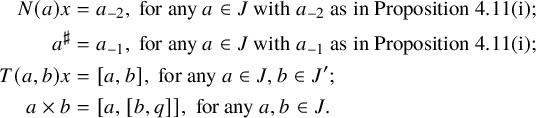 $$ \begin{align*} N(a)x &= a_{-2}, \text{ for any } a\in J \text{ with } a_{-2} \text{ as in Proposition~4.11(i)};\\ a^\sharp &= a_{-1}, \text{ for any } a\in J \text{ with } a_{-1} \text{ as in Proposition~4.11(i)};\\ T(a,b)x &= [a,b], \text{ for any } a\in J, b\in J';\\ a\times b &= [a,[b,q]], \text{ for any } a, b\in J. \end{align*} $$
Note that T is a bilinear map and that $\times $
is a symmetric bilinear map because
$\times $
is a symmetric bilinear map because $[J,J]=0$
. Similarly, we define maps
$[J,J]=0$
. Similarly, we define maps $N' \colon J'\to k$
,
$N' \colon J'\to k$
, $\sharp ' \colon J'\to J$
,
$\sharp ' \colon J'\to J$
, $T' \colon J'\times J \to k$
and
$T' \colon J'\times J \to k$
and $\times ' \colon J'\times J'\to J$
:
$\times ' \colon J'\times J'\to J$
:
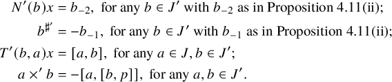 $$ \begin{align*} N'(b)x &= b_{-2}, \text{ for any } b\in J' \text{ with } b_{-2} \text{ as in Proposition~4.11(ii)}; \\ b^{\sharp'} &= -b_{-1}, \text{ for any } b\in J' \text{ with } b_{-1} \text{ as in Proposition~4.11(ii)}; \\ T'(b,a)x &= [a,b], \text{ for any } a\in J, b\in J';\\ a\times' b &= -[a,[b,p]], \text{ for any } a, b\in J'. \end{align*} $$
(Notice the two minus signs. Observe that $T'(b,a) = T(a,b)$
for all
$T'(b,a) = T(a,b)$
for all $a \in J$
,
$a \in J$
, $b \in J'$
.)
$b \in J'$
.)
Using Proposition 4.11, we can deduce some identities.
Lemma 4.13. Let $a,b\in J$
and
$a,b\in J$
and $\lambda \in k$
. Then
$\lambda \in k$
. Then
 $$ \begin{align} (\lambda a)^\sharp &=\lambda^2a^\sharp; \end{align} $$
 $$ \begin{align} N(\lambda a) &=\lambda^3 N(a); \end{align} $$
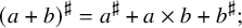 $$ \begin{align} (a+b)^\sharp &=a^\sharp+a\times b+b^\sharp; \end{align} $$
 $$ \begin{align} N(a+b) &=N(a)+T(b,a^\sharp)+T(a,b^\sharp)+N(b); \end{align} $$
 $$ \begin{align} (a^\sharp)^{\sharp'}&=N(a)a; \end{align} $$
 $$ \begin{align} N'(a^\sharp) &= N(a)^2. \end{align} $$
Similar identities hold for $a,b \in J'$
.
$a,b \in J'$
.
Proof. Equations (30) and (31) follow immediately from Proposition 4.11 and Theorem 3.13(vii).
Now let $a,b \in J$
and consider the corresponding automorphisms
$a,b \in J$
and consider the corresponding automorphisms $\alpha $
for a and
$\alpha $
for a and $\beta $
for b as in Proposition 4.11. Then
$\beta $
for b as in Proposition 4.11. Then $\alpha (q)=N(a)x+a^\sharp +[a,q]+q$
and
$\alpha (q)=N(a)x+a^\sharp +[a,q]+q$
and $\beta (q)=N(b)x+b^\sharp +[b,q]+q$
. The elements
$\beta (q)=N(b)x+b^\sharp +[b,q]+q$
. The elements $\alpha \beta (q)$
and
$\alpha \beta (q)$
and $\beta \alpha (q)$
are also extremal, and
$\beta \alpha (q)$
are also extremal, and
 $$ \begin{align*} \alpha\beta(q) &= \big( N(b)x+T(a,b^\sharp)x+q_{\alpha}([b,q])+N(a)x \big) + (b^\sharp+a\times b+a^\sharp )+[b+a,q]+q, \\ \beta\alpha(q) &= \big( N(a)x+T(b,a^\sharp)x+q_{\beta}([a,q])+N(b)x \big) + (a^\sharp+b\times a+b^\sharp )+[a+b,q]+q. \end{align*} $$
Since $a^\sharp + a\times b + b^\sharp \in J'$
, we can use the uniqueness in Proposition 4.11 applied on
$a^\sharp + a\times b + b^\sharp \in J'$
, we can use the uniqueness in Proposition 4.11 applied on $a+b \in J$
to obtain (32) and
$a+b \in J$
to obtain (32) and
 $$ \begin{align*} N(a+b)x&=N(a)x+T(b,a^\sharp)x+q_{\beta}([a,q])+N(b)x\\ &=N(a)x+T(a,b^\sharp)x+q_{\alpha}([b,q])+N(b)x. \end{align*} $$
In particular, we have
 $$ \begin{align} T(a,b^\sharp)x - q_{\beta}([a,q]) = T(b,a^\sharp)x - q_{\alpha}([b,q]). \end{align} $$
Since $b\in J$
is arbitrary, we can replace it by
$b\in J$
is arbitrary, we can replace it by $\lambda b$
for arbitrary
$\lambda b$
for arbitrary $\lambda \in k$
. By Theorem 3.13(vii), (30), and the linearity of T, the left-hand side of (36) is quadratic in
$\lambda \in k$
. By Theorem 3.13(vii), (30), and the linearity of T, the left-hand side of (36) is quadratic in $\lambda $
, while the right-hand side is linear in
$\lambda $
, while the right-hand side is linear in $\lambda $
. Since
$\lambda $
. Since $|k|\geq 3$
, this implies that both the left- and the right-hand side of (36) are
$|k|\geq 3$
, this implies that both the left- and the right-hand side of (36) are $0$
. So we obtain (33).
$0$
. So we obtain (33).
We now show (34) and (35) simultaneously. Let $a\in J$
be arbitrary and consider the corresponding extremal element
$a\in J$
be arbitrary and consider the corresponding extremal element $e = N(a)x + a^\sharp + [a,q] + q$
. Since
$e = N(a)x + a^\sharp + [a,q] + q$
. Since $a^\sharp \in J' \leq L_0'$
and
$a^\sharp \in J' \leq L_0'$
and $p \in L^{\prime }_{-1}$
, we get
$p \in L^{\prime }_{-1}$
, we get $g(p, a^\sharp ) = 0$
by Lemma 2.15. Notice that
$g(p, a^\sharp ) = 0$
by Lemma 2.15. Notice that $e \in L^{\prime \prime }_{-1}$
, so
$e \in L^{\prime \prime }_{-1}$
, so $(e,p) \in E_1$
because of the grading (18). It follows that
$(e,p) \in E_1$
because of the grading (18). It follows that
 $$\begin{align*}[e, p] = -N(a)c + [a^\sharp,p] + [[a,q],p] + y \in E. \end{align*}$$
Notice that $[[a,q],p] = [a,y]$
by the Jacobi identity, since
$[[a,q],p] = [a,y]$
by the Jacobi identity, since $[a,p] \in [J,p] = 0$
. Applying the automorphism
$[a,p] \in [J,p] = 0$
. Applying the automorphism $\varphi $
from Lemma 2.8, we get
$\varphi $
from Lemma 2.8, we get
 $$\begin{align*}x + [x,[a,y]] + \varphi([a^\sharp,p]) - N(a)p \in E. \end{align*}$$
Recall that $\varphi (l_0) = l_0 + [x, [y, l_0]]$
for all
$\varphi (l_0) = l_0 + [x, [y, l_0]]$
for all $l_0 \in L_0$
. However,
$l_0 \in L_0$
. However, $[y, [a^\sharp , p]] = 0$
because of the grading (see again Figure 1), so
$[y, [a^\sharp , p]] = 0$
because of the grading (see again Figure 1), so $\varphi ([a^\sharp ,p]) = [a^\sharp , p]$
. Combined with
$\varphi ([a^\sharp ,p]) = [a^\sharp , p]$
. Combined with $[x, [a,y]] = a$
by Proposition 2.4(iii), we get
$[x, [a,y]] = a$
by Proposition 2.4(iii), we get
 $$\begin{align*}x + a + [a^\sharp,p] - N(a)p \in E. \end{align*}$$
First, assume $N(a)\neq 0$
. Applying the automorphism
$N(a)\neq 0$
. Applying the automorphism $\varphi _\lambda $
from Lemma 2.10 with
$\varphi _\lambda $
from Lemma 2.10 with $\lambda = -N(a)^{-1}$
, we get
$\lambda = -N(a)^{-1}$
, we get
 $$\begin{align*}N(a)^2 x - N(a) a + [a^\sharp,p] + p \in E. \end{align*}$$
By definition of $\sharp '$
, this implies
$\sharp '$
, this implies $(a^\sharp )^{\sharp '}=N(a)a$
and
$(a^\sharp )^{\sharp '}=N(a)a$
and $N'(a^\sharp ) = N(a)^2$
, so we obtain (34) and (35) if
$N'(a^\sharp ) = N(a)^2$
, so we obtain (34) and (35) if $N(a)\neq 0$
.
$N(a)\neq 0$
.
Now assume $N(a)=0$
. If
$N(a)=0$
. If $a^\sharp =0$
, then (34) and (35) are trivially satisfied, so assume
$a^\sharp =0$
, then (34) and (35) are trivially satisfied, so assume $a^\sharp \neq 0$
. Then
$a^\sharp \neq 0$
. Then
 $$\begin{align*}e = a^\sharp + [a,q] + q. \end{align*}$$
In particular, $e \in L_{\geq -1} \setminus L_{\geq 0}$
, so by Proposition 2.5, we get
$e \in L_{\geq -1} \setminus L_{\geq 0}$
, so by Proposition 2.5, we get $(e, y) \in E_1$
and hence,
$(e, y) \in E_1$
and hence, $[a^\sharp ,y]=[e,y]\in E$
. It follows that also
$[a^\sharp ,y]=[e,y]\in E$
. It follows that also $a^\sharp = [x,[a^\sharp ,y]] \in E$
. Since
$a^\sharp = [x,[a^\sharp ,y]] \in E$
. Since $g(p, a^\sharp ) = 0$
, it follows that
$g(p, a^\sharp ) = 0$
, it follows that $\exp (a^\sharp )(p) = [a^\sharp ,p] + p \in E$
, and thus,
$\exp (a^\sharp )(p) = [a^\sharp ,p] + p \in E$
, and thus, $(a^\sharp )^{\sharp '}=0$
and
$(a^\sharp )^{\sharp '}=0$
and $N'(a^\sharp )=0$
, proving (34) and (35) also in this case.
$N'(a^\sharp )=0$
, proving (34) and (35) also in this case.
Lemma 4.14. For all $a,b,c\in J$
, we have
$a,b,c\in J$
, we have
 $$ \begin{align} T(a,a^\sharp)&=3N(a);\end{align} $$
 $$ \begin{align} a\times a &=2a^\sharp; \end{align} $$
 $$ \begin{align} T(c,a\times b)&=T(a,b\times c); \end{align} $$
 $$ \begin{align} a^\sharp\times'(a\times b)&=N(a)b+T(b,a^\sharp)a; \end{align} $$
 $$ \begin{align} a^\sharp\times'b^\sharp &=-(a\times b)^{\sharp'}+T(b,a^\sharp)b+T(a,b^\sharp)a. \end{align} $$
Similar identities hold for $a,b,c \in J'$
.
$a,b,c \in J'$
.
Proof. By (30) to (35), this follows in exactly the same way as in [Reference Tits and WeissTW02, (15.16), (15.18)]. (Recall from Assumption 4.1 that we assume $|k| \geq 4$
.)
$|k| \geq 4$
.)
Remark 4.15. The identities (30) to (35) and (37) to (41) we have shown so far may serve as an axiom system for ‘cubic norm pairs’ $(J, J')$
. Although this seems to be a natural counterpart for cubic norm structures in the context of Jordan pairs (rather than Jordan algebras), this notion seems to have appeared only once in the literature in a paper by John Faulkner [Reference FaulknerFau01], although the setup of a paired structure also appears already in [Reference SpringerSpr62]. (We thank Holger Petersson for pointing this out to us.) A recent contribution to the theory of cubic norm pairs, also related to
$(J, J')$
. Although this seems to be a natural counterpart for cubic norm structures in the context of Jordan pairs (rather than Jordan algebras), this notion seems to have appeared only once in the literature in a paper by John Faulkner [Reference FaulknerFau01], although the setup of a paired structure also appears already in [Reference SpringerSpr62]. (We thank Holger Petersson for pointing this out to us.) A recent contribution to the theory of cubic norm pairs, also related to $G_2$
-graded Lie algebras, is Michiel Smet’s preprint [Reference SmetSme25].
$G_2$
-graded Lie algebras, is Michiel Smet’s preprint [Reference SmetSme25].
At this point, we have, in principle, gathered enough information to reconstruct the Lie algebra from our data. Since this is not our main focus, we will only sketch the procedure. We will need the following concrete computations, providing us with information about the Lie bracket with the ‘middle part’ $L_0 \cap L^{\prime }_0$
, which is the most difficult piece to control. (Notice that
$L_0 \cap L^{\prime }_0$
, which is the most difficult piece to control. (Notice that $[J, [y, J']]$
and
$[J, [y, J']]$
and $[J', [y, J]]$
belong to this middle part.)
$[J', [y, J]]$
belong to this middle part.)
Lemma 4.16. Let $a,b,e \in J$
and
$a,b,e \in J$
and $a',b',e' \in J'$
be arbitrary. Then
$a',b',e' \in J'$
be arbitrary. Then
 $$ \begin{align} [a,[b,[y,e]]] &= T(a, b \times e)c;\end{align} $$
 $$ \begin{align} [a',[b',[y,e']]] &= T(b' \times' e', a')d; \end{align} $$
 $$ \begin{align} [a,[b',[y,e']]] &= - a \times (b' \times' e'); \end{align} $$
 $$ \begin{align} [a',[b,[y,e]]] &= a' \times' (b \times e); \end{align} $$
 $$ \begin{align} [a,[b',[y,e]]] &= b' \times' (a \times e) - T(a, b')e; \end{align} $$
 $$ \begin{align} [a',[b,[y,e']]] &= - b \times (a' \times' e') + T(b, a')e; \end{align} $$
 $$ \begin{align} [a,[b,[y,e']]] &= e' \times' (a \times b) - T(a, e')b - T(b, e')a; \end{align} $$
 $$ \begin{align} [a',[b',[y,e]]] &= - e \times (a' \times' b') + T(e, a')b' + T(e, b')a'. \end{align} $$
Proof. By the grading (see Figure 1), we have $[a,[b,[y,e]]] \in L_{-1} \cap L^{\prime }_{-2} = \langle c \rangle $
, so
$[a,[b,[y,e]]] \in L_{-1} \cap L^{\prime }_{-2} = \langle c \rangle $
, so $[a,[b,[y,e]]] = \lambda c$
for some
$[a,[b,[y,e]]] = \lambda c$
for some $\lambda \in k$
. Since
$\lambda \in k$
. Since $[c,d]=x$
and
$[c,d]=x$
and $[J,d]=0$
, we get
$[J,d]=0$
, we get
 $$\begin{align*}\lambda x = [d,[a,[b,[e,y]]]] = [a,[b,[e,[d,y]]]] = [a,[b,[e,q]]] = [a, b\times e] = T(a, b \times e)x, \end{align*}$$
and hence, (42) holds. The proof of (43) is similar.
Next, since $y = [q,p]$
,
$y = [q,p]$
, $[q, e'] = 0$
and
$[q, e'] = 0$
and $[q, b'] = 0$
, we get
$[q, b'] = 0$
, we get
 $$ \begin{align*} [a, [b', [y, e']]] & = [a, [b', [[q, p], e']]] \\ & = [a, [b', [q, [p, e']]]] \\ & = [a, [q, [b', [p, e']]]] = - a \times (b' \times' e'), \end{align*} $$
proving (44). The proof of (45) is similar.
Now, by the Jacobi identity and (45), we have
 $$\begin{align*}[a, [b', [y, e]]] = [b', [a, [y,e]]] + [[a,b'], [y,e]] = b' \times' (a \times e) + [T(a,b')x, [y,e]], \end{align*}$$
so we get (46). The proof of (47) is similar.
Finally, by applying the Jacobi identity twice and using $[a,[b,e']] \in L_{-3}=0$
and (46), we get
$[a,[b,e']] \in L_{-3}=0$
and (46), we get
 $$ \begin{align*} [a,[b,[y,e']]] &= [y,[a,[b,e']]] + [a,[[b,y],e']] + [[a,y],[b,e']] \\ &= 0 + [a, [e', [y, b]]] + [[a,y], T(b,e')x] \\ &= e' \times' (a \times b) - T(a, e')b - T(b, e')a, \end{align*} $$
Here is the promised sketch of the reconstruction result.
Corollary 4.17. The Lie bracket on L can be completely recovered from the maps T, $\times $
and
$\times $
and $\times '$
alone.
$\times '$
alone.
Proof. Notice that, by Figure 1, the algebra L has a decomposition into $13$
pieces. Now let
$13$
pieces. Now let
 $$\begin{align*}K_0 := \langle [x,y], [q,c] \rangle \oplus [J, [y, J']] , \end{align*}$$
and let K be the subspace of L spanned by $K_0$
together with the
$K_0$
together with the $12$
remaining pieces of L. It is not difficult to check (but it requires some case analysis) that K is an ideal of L. Since L is simple, it follows that
$12$
remaining pieces of L. It is not difficult to check (but it requires some case analysis) that K is an ideal of L. Since L is simple, it follows that $K = L$
, so in particular,
$K = L$
, so in particular, $K_0 = L_0 \cap L^{\prime }_0$
. Now observe that we can identify
$K_0 = L_0 \cap L^{\prime }_0$
. Now observe that we can identify $K_0$
with the Lie algebra
$K_0$
with the Lie algebra $\tilde K_0$
consisting of the corresponding inner derivations
$\tilde K_0$
consisting of the corresponding inner derivations $\operatorname {\mathrm {ad}}_l$
(for each
$\operatorname {\mathrm {ad}}_l$
(for each $l \in K_0$
) restricted to the sum of the
$l \in K_0$
) restricted to the sum of the $12$
remaining pieces; see, for example, [Reference Boelaert, De Medts and StavrovaBDMS19, Construction 4.1.2]. (Since L is simple, the corresponding Lie algebra homomorphism
$12$
remaining pieces; see, for example, [Reference Boelaert, De Medts and StavrovaBDMS19, Construction 4.1.2]. (Since L is simple, the corresponding Lie algebra homomorphism $K_0 \to \tilde K_0$
is injective and hence an isomorphism.)
$K_0 \to \tilde K_0$
is injective and hence an isomorphism.)
The Lie algebra L can now be reconstructed from six one-dimensional subspaces, three copies of J, three copies of $J'$
, and a copy of
$J'$
, and a copy of $\tilde K_0$
, assembled exactly as in Figure 1. It is now a routine (but somewhat lengthy) verification, relying on Lemma 4.16, that that the Lie bracket between every two of the
$\tilde K_0$
, assembled exactly as in Figure 1. It is now a routine (but somewhat lengthy) verification, relying on Lemma 4.16, that that the Lie bracket between every two of the $13$
pieces is completey determined by the maps T,
$13$
pieces is completey determined by the maps T, $\times $
and
$\times $
and $\times '$
.
$\times '$
.
So far, we have been able to endow the pair $(J, J')$
with a ‘twin cubic norm structure’ using the various maps between them. (See also Remark 4.15.) When the norm N is not identically zero, we can go one step further, by selecting a ‘base point’ to identify the two parts of this twin structure, which then results in a genuine cubic norm structure.
$(J, J')$
with a ‘twin cubic norm structure’ using the various maps between them. (See also Remark 4.15.) When the norm N is not identically zero, we can go one step further, by selecting a ‘base point’ to identify the two parts of this twin structure, which then results in a genuine cubic norm structure.
Lemma 4.18. If $N\neq 0$
, then we can re-choose c and d in Notation 4.2 in such a way that
$N\neq 0$
, then we can re-choose c and d in Notation 4.2 in such a way that $N(z)=1$
for some
$N(z)=1$
for some $z \in J$
. We call z a base point for N.
$z \in J$
. We call z a base point for N.
Proof. Let $z\in J$
such that
$z\in J$
such that $N(z)\neq 0$
. If we replace c by
$N(z)\neq 0$
. If we replace c by $\tilde c = N(z)c$
and d by
$\tilde c = N(z)c$
and d by $\tilde d = N(z)^{-1}d$
in Notation 4.2, and correspondingly replace p by
$\tilde d = N(z)^{-1}d$
in Notation 4.2, and correspondingly replace p by $\tilde p = N(z)p$
and q by
$\tilde p = N(z)p$
and q by $\tilde q = N(z)^{-1}q$
, then all conditions in Notation 4.2 remain satisfied. Since we have only replaced these elements by a scalar multiple, this does not affect any of the decompositions.
$\tilde q = N(z)^{-1}q$
, then all conditions in Notation 4.2 remain satisfied. Since we have only replaced these elements by a scalar multiple, this does not affect any of the decompositions.
Now denote the norm obtained from Definition 4.12 with these new choices by $\tilde N$
. Since
$\tilde N$
. Since $N(z)x+z^\sharp +[z,q]+q\in E$
, we get
$N(z)x+z^\sharp +[z,q]+q\in E$
, we get $x+N(z)^{-1}z^\sharp +[z, \tilde q] + \tilde q\in E$
, and it follows that indeed
$x+N(z)^{-1}z^\sharp +[z, \tilde q] + \tilde q\in E$
, and it follows that indeed $\tilde N(z)=1$
.
$\tilde N(z)=1$
.
Assume for the rest of this section that $N\neq 0$
and that
$N\neq 0$
and that $z \in J$
is a base point for N.
$z \in J$
is a base point for N.
Definition 4.19. We define maps $\sigma \colon J\to J'$
and
$\sigma \colon J\to J'$
and $\sigma ' \colon J'\to J$
by
$\sigma ' \colon J'\to J$
by
 $$ \begin{align*} \sigma(a) &= T(a,z^\sharp)z^\sharp - z\times a, \\ \sigma'(b) &= T(z,b)z - b \times' z^\sharp, \end{align*} $$
for all $a \in J$
and all
$a \in J$
and all $b \in J'$
.
$b \in J'$
.
Lemma 4.20. We have $\sigma '\circ \sigma =\operatorname {\mathrm {id}}_J$
and
$\sigma '\circ \sigma =\operatorname {\mathrm {id}}_J$
and $\sigma \circ \sigma '=\operatorname {\mathrm {id}}_{J'}$
.
$\sigma \circ \sigma '=\operatorname {\mathrm {id}}_{J'}$
.
Proof. Let $a \in J$
be arbitrary. Then by (34) and (37) to (40) and since
$a \in J$
be arbitrary. Then by (34) and (37) to (40) and since $N(z)=1$
,
$N(z)=1$
,
 $$ \begin{align*} \sigma'(\sigma(a))&= T(z,T(a,z^\sharp)z^\sharp)z-T(z,z\times a)z-T(a,z^\sharp)z^\sharp\times'z^\sharp+ (z\times a) \times' z^\sharp \\ &= T(a,z^\sharp)T(z,z^\sharp)z-T(a,z\times z)z-2T(a,z^\sharp)(z^\sharp)^{\sharp'} +N(z)a+T(a,z^\sharp)z \\ &= 3T(a,z^\sharp)z-2T(a,z^\sharp)z-2T(a,z^\sharp)z +a+T(a,z^\sharp)z \\ &= a. \end{align*} $$
The proof of the second equality is similar.
Lemma 4.21. We have $\sigma '\circ \sharp =\sharp '\circ \sigma $
.
$\sigma '\circ \sharp =\sharp '\circ \sigma $
.
Proof. Let $a \in J$
be arbitrary. On the one hand, using (41), we get
$a \in J$
be arbitrary. On the one hand, using (41), we get
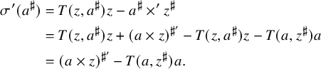 $$ \begin{align*} \sigma'(a^\sharp)&=T(z,a^\sharp)z-a^\sharp\times' z^\sharp \\ &=T(z,a^\sharp)z+(a\times z)^{\sharp'}-T(z,a^\sharp)z-T(a,z^\sharp)a \\ &=(a\times z)^{\sharp'}-T(a,z^\sharp)a. \end{align*} $$
On the other hand, using $N(z)=1$
, (30), (32), (34) and (40), we have
$N(z)=1$
, (30), (32), (34) and (40), we have
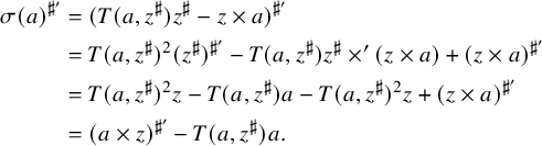 $$ \begin{align*} \sigma(a)^{\sharp'}&=(T(a,z^\sharp)z^\sharp-z\times a)^{\sharp'} \\ &=T(a,z^\sharp)^2(z^\sharp)^{\sharp'}-T(a,z^\sharp)z^\sharp\times'(z\times a)+(z\times a)^{\sharp'} \\ &=T(a,z^\sharp)^2z-T(a,z^\sharp)a-T(a,z^\sharp)^2z+(z\times a)^{\sharp'}\\ &=(a\times z)^{\sharp'}-T(a,z^\sharp)a. \end{align*} $$
We are now ready to define the cubic norm structure and prove the required defining identities; see Definition 1.11.
Definition 4.22. We define maps $T_J:J\times J\to k$
,
$T_J:J\times J\to k$
, $\times _J:J\times J\to J$
and
$\times _J:J\times J\to J$
and $\sharp _J:J\to J$
by setting
$\sharp _J:J\to J$
by setting
 $$ \begin{align} T_J(a,b) &= T(a,\sigma(b)), \end{align} $$
 $$ \begin{align} a\times_J b &= \sigma'(a\times b) = \sigma(a) \times' \sigma(b), \end{align} $$
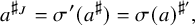 $$ \begin{align} a^{\sharp_J} &= \sigma'(a^\sharp) = \sigma(a)^{\sharp'}, \end{align} $$
for all $a,b \in J$
. (The rightmost equalities in (51) and (52) hold by Lemma 4.21.)
$a,b \in J$
. (The rightmost equalities in (51) and (52) hold by Lemma 4.21.)
Theorem 4.23. Let L be as in Notation 4.2 and J be as in Notation 4.4. Assume that the map N defined in Definition 4.12 is not identically zero. Then the data $(J,k,N,\sharp _J, T_J,\times _J,z)$
forms a nondegenerate cubic norm structure.
$(J,k,N,\sharp _J, T_J,\times _J,z)$
forms a nondegenerate cubic norm structure.
Proof. Recall that by Lemma 1.13, we only have to show that the defining identities (i), (ii), (iv), (v), (vii), (x) and (xi) of Definition 1.11 are satisfied.
First, note that $\times _J$
is symmetric and bilinear by construction. For
$\times _J$
is symmetric and bilinear by construction. For $T_J$
, we have
$T_J$
, we have
 $$ \begin{align*} T_J(a,b)&=T(a,T(b,z^\sharp)z^\sharp)-T(a,z\times b)=T(a,z^\sharp)T(b,z^\sharp)-T(z,a\times b) \end{align*} $$
by (39), and hence, $T_J$
is symmetric and bilinear.
$T_J$
is symmetric and bilinear.
Identity (i) follows from the linearity of $\sigma '$
and (30). Identity (ii) is precisely (31). Identity (iv) follows from the linearity of
$\sigma '$
and (30). Identity (ii) is precisely (31). Identity (iv) follows from the linearity of $\sigma '$
and (32). Identity (v) follows from Lemma 4.20 and (33). Identity (vii) follows from Lemmas 4.20 and 4.21 and (34). Identity (x) follows from
$\sigma '$
and (32). Identity (v) follows from Lemma 4.20 and (33). Identity (vii) follows from Lemmas 4.20 and 4.21 and (34). Identity (x) follows from
 $$\begin{align*}\sigma'(z^\sharp)=T(z,z^\sharp)z-z^\sharp\times'z^\sharp=3N(z)z-2N(z)z=z, \end{align*}$$
using (34), (37) and (38) and $N(z)=1$
. Identity (xi) follows from
$N(z)=1$
. Identity (xi) follows from
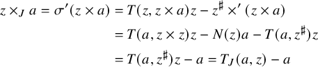 $$ \begin{align*} z \times_J a=\sigma'(z\times a)&=T(z,z\times a)z-z^\sharp \times' (z\times a) \\ &=T(a,z\times z)z-N(z)a-T(a,z^\sharp)z \\ &=T(a,z^\sharp)z-a=T_J(a,z)-a \end{align*} $$
for all $a \in J$
, using (38) to (40),
$a \in J$
, using (38) to (40), $\sigma (z)=z^\sharp $
and
$\sigma (z)=z^\sharp $
and $N(z)=1$
. Finally, the cubic norm structure is nondegenerate: if
$N(z)=1$
. Finally, the cubic norm structure is nondegenerate: if $a \in J$
is such that
$a \in J$
is such that $T_J(a, J) = 0$
, then we have
$T_J(a, J) = 0$
, then we have $T(a, J') = 0$
(i.e.,
$T(a, J') = 0$
(i.e., $[a, J'] = 0$
), but it then follows from the grading that
$[a, J'] = 0$
), but it then follows from the grading that $[a, L_{-1}] = 0$
; Lemma 2.11 then implies that
$[a, L_{-1}] = 0$
; Lemma 2.11 then implies that $a=0$
.
$a=0$
.
Remark 4.24. A different choice of base point would give rise to a different cubic norm structure, but it is not hard to show (and not surprising) that the resulting cubic norm structures are isotopic; see Definition 1.15.
Remark 4.25. If the cubic norm structure is anisotropic (see Definition 1.12), then the extremal geometry is, in fact, a generalized hexagon. (The key point here is the fact that the extremal geometry is a generalized hexagon if and only if there are no symplectic pairs, a fact that we have exploited already in the proof of Lemma 3.3. The existence of symplecta turns out to be equivalent to the existence of extremal elements in $L^{\prime }_{-1} \cap L_{-1} = J$
, and such elements always have norm
$L^{\prime }_{-1} \cap L_{-1} = J$
, and such elements always have norm $0$
.)
$0$
.)
With some more effort, we can use the techniques developed in this section to show that this generalized hexagon is isomorphic to the Moufang hexagon obtained from the cubic norm structure as in [Reference Tits and WeissTW02, (16.8)], and we can determine the root groups and the commutator relations explicitly in terms of the Lie algebra. Since this result is not so surprising but still requires a substantial amount of work, we omit the details. See [Reference MeulewaeterMeu21, §4.4.2].
Remark 4.26. If the map N is identically zero, then also the maps $\sharp $
,
$\sharp $
, $\times $
,
$\times $
, $N'$
,
$N'$
, $\sharp '$
and
$\sharp '$
and $\times '$
are identically zero. In this case, it can be shown that the extremal geometry is isomorphic to a geometry of the form
$\times '$
are identically zero. In this case, it can be shown that the extremal geometry is isomorphic to a geometry of the form $\Gamma (V, W^*)$
as defined in [Reference Cuypers and MeulewaeterCM21, Example 2.8]. Note that these examples also occur when the Lie algebra is infinite-dimensional. In the finite-dimensional case, these are precisely so-called root shadow spaces of type
$\Gamma (V, W^*)$
as defined in [Reference Cuypers and MeulewaeterCM21, Example 2.8]. Note that these examples also occur when the Lie algebra is infinite-dimensional. In the finite-dimensional case, these are precisely so-called root shadow spaces of type $A_{n, \{1,n\}}$
.
$A_{n, \{1,n\}}$
.
5 Extremal geometry with symplectic pairs – recovering a quadrangular algebra
In this section, we continue to assume that L is a simple Lie algebra generated by its pure extremal elements, but we make different assumptions on the existence of certain extremal elements and extremal lines.
Assumption 5.1. We assume that L is a simple Lie algebra, defined over a field k with $|k|>2$
, such that L is generated by its set E of pure extremal elements, and such that
$|k|>2$
, such that L is generated by its set E of pure extremal elements, and such that
-
(i) there exists a Galois extension
$k'/k$
of degree at most
$2$
such that the extremal geometry of
$L\otimes k'$
contains lines; -
(ii) there exist symplectic pairs of extremal elements.


This time, we will show that $L_{-1}$
can be decomposed as
$L_{-1}$
can be decomposed as $V \oplus X \oplus V'$
into
$V \oplus X \oplus V'$
into $3$
parts, where
$3$
parts, where $V' \cong V$
, and that
$V' \cong V$
, and that $(V,X)$
can be made into a quadrangular algebra. This will require a substantial amount of work, mostly because we are including the case
$(V,X)$
can be made into a quadrangular algebra. This will require a substantial amount of work, mostly because we are including the case $\operatorname {\mathrm {char}}(k)=2$
. Notice, however, that we will never require a case distinction, not even in the computations in our proofs. For convenience, we have included the
$\operatorname {\mathrm {char}}(k)=2$
. Notice, however, that we will never require a case distinction, not even in the computations in our proofs. For convenience, we have included the $\operatorname {\mathrm {char}}(k)\neq 2$
description of
$\operatorname {\mathrm {char}}(k)\neq 2$
description of $\theta $
in Proposition 5.30, but we never use this result.
$\theta $
in Proposition 5.30, but we never use this result.
We first point out that L remains simple after base extension to $k'$
.
$k'$
.
Lemma 5.2. The Lie algebra $L_{k'} := L \otimes _k k'$
is simple.
$L_{k'} := L \otimes _k k'$
is simple.
Proof. Essentially, this is shown in the proof of [Reference Cuypers and MeulewaeterCM21, Theorem 5.7]. However, the statement in loc. cit. assumes $\operatorname {\mathrm {char}}(k) \neq 2$
, and extending it to all characteristics requires some subtle changes in the final step, so we give a complete proof.
$\operatorname {\mathrm {char}}(k) \neq 2$
, and extending it to all characteristics requires some subtle changes in the final step, so we give a complete proof.
Let $\sigma $
be the unique nontrivial element of
$\sigma $
be the unique nontrivial element of $\operatorname {\mathrm {Gal}}(k'/k)$
. We first recallFootnote 3 that, by Speiser’s Lemma (see, for example, [Reference Gille and SzamuelyGS17, Lemma 2.3.8]), each
$\operatorname {\mathrm {Gal}}(k'/k)$
. We first recallFootnote 3 that, by Speiser’s Lemma (see, for example, [Reference Gille and SzamuelyGS17, Lemma 2.3.8]), each $\sigma $
-invariant subspace W of
$\sigma $
-invariant subspace W of $L_{k'}$
can be written as
$L_{k'}$
can be written as $W = V \otimes _k k'$
for some subspace V of L.
$W = V \otimes _k k'$
for some subspace V of L.
Now let I be a nontrivial ideal of $L_{k'}$
and let
$L_{k'}$
and let $a \in I$
with
$a \in I$
with $a \neq 0$
. Then, as the extremal elements in E linearly span L, they also span
$a \neq 0$
. Then, as the extremal elements in E linearly span L, they also span $L_{k'}$
over
$L_{k'}$
over $k'$
, so we can write
$k'$
, so we can write
 $$\begin{align*}a = x_1 \otimes \lambda_1+\cdots+x_k\otimes \lambda_k, \end{align*}$$
where $x_j \in E$
are linearly independent and each
$x_j \in E$
are linearly independent and each $\lambda _j \in k^{\prime \times }$
. After replacing a with a scalar multiple, we can assume
$\lambda _j \in k^{\prime \times }$
. After replacing a with a scalar multiple, we can assume $\lambda _1+\lambda _1^\sigma \neq 0$
. Then
$\lambda _1+\lambda _1^\sigma \neq 0$
. Then $a+a^\sigma $
is a nontrivial element in
$a+a^\sigma $
is a nontrivial element in $I+I^\sigma $
fixed by
$I+I^\sigma $
fixed by $\sigma $
. Therefore, the subspace spanned by the elements in
$\sigma $
. Therefore, the subspace spanned by the elements in $I+I^\sigma $
fixed by
$I+I^\sigma $
fixed by $\sigma $
forms a nontrivial ideal of L, which by simplicity of L equals L. This implies that
$\sigma $
forms a nontrivial ideal of L, which by simplicity of L equals L. This implies that $I+I^\sigma = L_{k'}$
.
$I+I^\sigma = L_{k'}$
.
Since both I and $I^\sigma $
are ideals,
$I^\sigma $
are ideals, $I\cap I^\sigma $
is an ideal which is stabilized by
$I\cap I^\sigma $
is an ideal which is stabilized by $\sigma $
. By Speiser’s Lemma,
$\sigma $
. By Speiser’s Lemma, $I \cap I^\sigma = V \otimes _k k'$
for some subspace V of L, but then V is an ideal of L. By the simplicity of L, this implies that either
$I \cap I^\sigma = V \otimes _k k'$
for some subspace V of L, but then V is an ideal of L. By the simplicity of L, this implies that either $I = L_{k'}$
, or
$I = L_{k'}$
, or $I\cap I^\sigma =0$
. So we may assume the latter, and therefore,
$I\cap I^\sigma =0$
. So we may assume the latter, and therefore, $L_{k'} = I \oplus I^\sigma $
. In particular,
$L_{k'} = I \oplus I^\sigma $
. In particular, $[I,I^\sigma ] \leq I \cap I^\sigma = 0$
, and thus,
$[I,I^\sigma ] \leq I \cap I^\sigma = 0$
, and thus,
 $$ \begin{align} [L_{k'}, L_{k'}] = [I,I]\oplus [I^\sigma,I^\sigma]. \end{align} $$
Since L is simple, $L=[L,L]$
and hence
$L=[L,L]$
and hence $L_{k'} = [L_{k'}, L_{k'}]$
, so it follows from (53) that
$L_{k'} = [L_{k'}, L_{k'}]$
, so it follows from (53) that $[I,I]=I$
.
$[I,I]=I$
.
Now let $x\in E$
be arbitrary. By the Premet identity (2) with
$x\in E$
be arbitrary. By the Premet identity (2) with $y,z \in I$
, we get
$y,z \in I$
, we get $g_x([y,z])x \in I$
for all
$g_x([y,z])x \in I$
for all $y,z \in I$
. Since
$y,z \in I$
. Since $I = [I,I]$
, it follows that
$I = [I,I]$
, it follows that $g_x(a) x \in I$
for all
$g_x(a) x \in I$
for all $a \in I$
. It thus follows that
$a \in I$
. It thus follows that $x \in I$
if we can find an
$x \in I$
if we can find an $a \in I$
with
$a \in I$
with $g(x,a) \neq 0$
. This is indeed always possible: since g is nondegenerate, there exists a
$g(x,a) \neq 0$
. This is indeed always possible: since g is nondegenerate, there exists a $y \in L$
with
$y \in L$
with $g(x,y) \neq 0$
, but since
$g(x,y) \neq 0$
, but since $L_{k'} = I + I^\sigma $
, we either find
$L_{k'} = I + I^\sigma $
, we either find $a \in I$
with
$a \in I$
with $g(x,a) \neq 0$
or we find
$g(x,a) \neq 0$
or we find $b \in I^\sigma $
with
$b \in I^\sigma $
with $g(x,b) \neq 0$
. In the latter case, however, we simply apply
$g(x,b) \neq 0$
. In the latter case, however, we simply apply $\sigma $
, and we find
$\sigma $
, and we find $g(x, b^\sigma ) \neq 0$
with
$g(x, b^\sigma ) \neq 0$
with $b^\sigma \in I$
.
$b^\sigma \in I$
.
Since $x\in E$
was arbitrary, we have shown that E is contained in I. However, E generates
$x\in E$
was arbitrary, we have shown that E is contained in I. However, E generates $L_{k'}$
, so we get that
$L_{k'}$
, so we get that $I = L_{k'}$
as required. (In fact, this is now a contradiction to the fact that
$I = L_{k'}$
as required. (In fact, this is now a contradiction to the fact that $I \cap I^\sigma = 0$
.)
$I \cap I^\sigma = 0$
.)
Proposition 5.3. There exist extremal elements x, y, c and d such that $g(x,y)=g(c,d)=1$
and
$g(x,y)=g(c,d)=1$
and $(x,c),(c,y),(y,d),(d,x) \in E_0$
.
$(x,c),(c,y),(y,d),(d,x) \in E_0$
.
Proof. Assume first that the extremal geometry of L contains lines. By Assumption 5.1(ii), there exists an $x\in E$
and a symplecton S of the extremal geometry containing
$x\in E$
and a symplecton S of the extremal geometry containing $\langle x\rangle $
. Recall from Assumption 3.1 that
$\langle x\rangle $
. Recall from Assumption 3.1 that $({\mathcal {E}}, {\mathcal {E}}_2)$
is connected, so there exist
$({\mathcal {E}}, {\mathcal {E}}_2)$
is connected, so there exist $y\in E$
such that
$y\in E$
such that $g(x,y)=1$
. By Proposition 3.5(v), there exists
$g(x,y)=1$
. By Proposition 3.5(v), there exists $c\in E$
such that
$c\in E$
such that $\langle c\rangle \in S$
and
$\langle c\rangle \in S$
and $(c,y)\in E_0$
. Since
$(c,y)\in E_0$
. Since $S \subseteq {\mathcal {E}}_{\leq 0}(x)$
, Proposition 2.13(iv) implies that also
$S \subseteq {\mathcal {E}}_{\leq 0}(x)$
, Proposition 2.13(iv) implies that also $(x,c)\in E_0$
.
$(x,c)\in E_0$
.
By Proposition 2.13(ii) applied on $(x,c)$
, there exists a symplecton T containing x and containing an extremal point hyperbolic with
$(x,c)$
, there exists a symplecton T containing x and containing an extremal point hyperbolic with $\langle c\rangle $
. By Proposition 3.5(v) again, we find
$\langle c\rangle $
. By Proposition 3.5(v) again, we find $d\in E$
such that
$d\in E$
such that $\langle d\rangle \in T$
with
$\langle d\rangle \in T$
with $(d,y) \in E_0$
, and again, Proposition 2.13(iv) implies that also
$(d,y) \in E_0$
, and again, Proposition 2.13(iv) implies that also $(d,x)\in E_0$
. It remains to show that
$(d,x)\in E_0$
. It remains to show that $(c,d)\in E_2$
. Let
$(c,d)\in E_2$
. Let $A := T \cap {\mathcal {E}}_{\leq 0}(c)$
. By Proposition 2.13(iv),
$A := T \cap {\mathcal {E}}_{\leq 0}(c)$
. By Proposition 2.13(iv), $A = T \cap {\mathcal {E}}_{0}(c)$
. By Proposition 3.5(v) now, A consists of the single point
$A = T \cap {\mathcal {E}}_{0}(c)$
. By Proposition 3.5(v) now, A consists of the single point $\langle x \rangle $
. We can now invoke [Reference Cuypers and MeulewaeterCM21, Lemma 2.17] to see that the point
$\langle x \rangle $
. We can now invoke [Reference Cuypers and MeulewaeterCM21, Lemma 2.17] to see that the point $\langle d \rangle $
is indeed contained in
$\langle d \rangle $
is indeed contained in ${\mathcal {E}}_2(c)$
. By rescaling c, we obtain
${\mathcal {E}}_2(c)$
. By rescaling c, we obtain $g(c,d)=1$
.
$g(c,d)=1$
.
Assume now that the extremal geometry of L does not contain lines. Then ${\mathcal {E}} \times {\mathcal {E}} = {\mathcal {E}}_{-2} \cup {\mathcal {E}}_0 \cup {\mathcal {E}}_2$
. By Assumption 5.1(i), the extremal geometry
${\mathcal {E}} \times {\mathcal {E}} = {\mathcal {E}}_{-2} \cup {\mathcal {E}}_0 \cup {\mathcal {E}}_2$
. By Assumption 5.1(i), the extremal geometry $\Gamma ' = ({\mathcal {E}}', \mathcal {F}')$
of
$\Gamma ' = ({\mathcal {E}}', \mathcal {F}')$
of $L_{k'}$
contains lines. Recall from Lemma 5.2 that
$L_{k'}$
contains lines. Recall from Lemma 5.2 that $L_{k'}$
is again simple, so it satisfies Assumption 3.1. Let
$L_{k'}$
is again simple, so it satisfies Assumption 3.1. Let $\operatorname {\mathrm {Gal}}(k'/k) = \langle \sigma \rangle $
. Then the involution
$\operatorname {\mathrm {Gal}}(k'/k) = \langle \sigma \rangle $
. Then the involution $\sigma $
also acts on
$\sigma $
also acts on $\Gamma '$
and fixes all points of
$\Gamma '$
and fixes all points of ${\mathcal {E}}$
.
${\mathcal {E}}$
.
We start now with a pair of extremal elements $(a,b) \in E_0$
. Recall from Assumption 3.1 that
$(a,b) \in E_0$
. Recall from Assumption 3.1 that $({\mathcal {E}}, {\mathcal {E}}_2)$
is connected, so there exist
$({\mathcal {E}}, {\mathcal {E}}_2)$
is connected, so there exist $e \in E$
such that
$e \in E$
such that $(a,e) \in E_2$
. Notice that by Proposition 3.5, there is a unique symplecton S through a and b in
$(a,e) \in E_2$
. Notice that by Proposition 3.5, there is a unique symplecton S through a and b in $\Gamma '$
, but since a and b are fixed by
$\Gamma '$
, but since a and b are fixed by $\sigma $
, also S is fixed (setwise) by
$\sigma $
, also S is fixed (setwise) by $\sigma $
. By Proposition 3.5(v), there is a unique point
$\sigma $
. By Proposition 3.5(v), there is a unique point $\langle x \rangle \in S$
in relation
$\langle x \rangle \in S$
in relation ${\mathcal {E}}^{\prime }_0$
with
${\mathcal {E}}^{\prime }_0$
with $\langle e \rangle $
. Then also
$\langle e \rangle $
. Then also $\langle x \rangle ^\sigma $
has this property, so we must have
$\langle x \rangle ^\sigma $
has this property, so we must have $\langle x \rangle ^\sigma = \langle x \rangle $
. By Hilbert’s Theorem 90, we may replace x by a
$\langle x \rangle ^\sigma = \langle x \rangle $
. By Hilbert’s Theorem 90, we may replace x by a $k'$
-multiple of x to get
$k'$
-multiple of x to get $x^\sigma = x$
and therefore
$x^\sigma = x$
and therefore $x \in E$
. Notice that now
$x \in E$
. Notice that now $(x, a) \in E_0$
and that S is the unique symplecton in
$(x, a) \in E_0$
and that S is the unique symplecton in $\Gamma '$
through
$\Gamma '$
through $\langle x \rangle $
and
$\langle x \rangle $
and $\langle a \rangle $
. We also have
$\langle a \rangle $
. We also have $(x, e) \in E_0$
; let T be the unique sympecton in
$(x, e) \in E_0$
; let T be the unique sympecton in $\Gamma '$
through
$\Gamma '$
through $\langle x \rangle $
and
$\langle x \rangle $
and $\langle e \rangle $
. Notice that
$\langle e \rangle $
. Notice that $S \cap T = \langle x \rangle $
.
$S \cap T = \langle x \rangle $
.
We now apply the connectedness of $({\mathcal {E}}, {\mathcal {E}}_2)$
again to find an element
$({\mathcal {E}}, {\mathcal {E}}_2)$
again to find an element $y \in E_2(x)$
. Then again, there is a unique point
$y \in E_2(x)$
. Then again, there is a unique point $\langle c \rangle \in S$
in relation
$\langle c \rangle \in S$
in relation ${\mathcal {E}}^{\prime }_0$
with y, and similarly, there is a unique point
${\mathcal {E}}^{\prime }_0$
with y, and similarly, there is a unique point $\langle d \rangle \in T$
in relation
$\langle d \rangle \in T$
in relation ${\mathcal {E}}^{\prime }_0$
with y. As before, we get
${\mathcal {E}}^{\prime }_0$
with y. As before, we get $\langle c \rangle ^\sigma = \langle c \rangle $
and
$\langle c \rangle ^\sigma = \langle c \rangle $
and $\langle d \rangle ^\sigma = \langle d \rangle $
, and we may rescale c and d so that
$\langle d \rangle ^\sigma = \langle d \rangle $
, and we may rescale c and d so that $c \in E$
and
$c \in E$
and $d \in E$
. Now observe that
$d \in E$
. Now observe that $(c,e) \not \in E_0$
, since otherwise both
$(c,e) \not \in E_0$
, since otherwise both $\langle x \rangle $
and
$\langle x \rangle $
and $\langle c \rangle $
would be in relation
$\langle c \rangle $
would be in relation ${\mathcal {E}}^{\prime }_0$
with
${\mathcal {E}}^{\prime }_0$
with $\langle e \rangle $
, contradicting Proposition 3.5(v) applied on S and e. Since
$\langle e \rangle $
, contradicting Proposition 3.5(v) applied on S and e. Since ${\mathcal {E}} \times {\mathcal {E}} = {\mathcal {E}}_{-2} \cup {\mathcal {E}}_0 \cup {\mathcal {E}}_2$
, this implies that
${\mathcal {E}} \times {\mathcal {E}} = {\mathcal {E}}_{-2} \cup {\mathcal {E}}_0 \cup {\mathcal {E}}_2$
, this implies that $(c,e) \in E_2$
. Similarly, it now follows that
$(c,e) \in E_2$
. Similarly, it now follows that $(c,d) \not \in E_0$
, since otherwise both
$(c,d) \not \in E_0$
, since otherwise both $\langle x \rangle $
and
$\langle x \rangle $
and $\langle d \rangle $
would be in relation
$\langle d \rangle $
would be in relation ${\mathcal {E}}^{\prime }_0$
with
${\mathcal {E}}^{\prime }_0$
with $\langle c \rangle $
, again contradicting Proposition 3.5(v), now applied on T and c. We conclude that
$\langle c \rangle $
, again contradicting Proposition 3.5(v), now applied on T and c. We conclude that $(c,d) \in E_2$
. It now only remains to rescale the elements to see that x, y, c and d satisfy all the required assumptions.
$(c,d) \in E_2$
. It now only remains to rescale the elements to see that x, y, c and d satisfy all the required assumptions.
Notation 5.4. Let x, y, c, d be as in Proposition 5.3. We denote the $5$
-grading on L associated with the hyperbolic pair
$5$
-grading on L associated with the hyperbolic pair $(x,y)$
as in Proposition 2.4 by
$(x,y)$
as in Proposition 2.4 by
 $$ \begin{align} L_{-2}\oplus L_{-1}\oplus L_0\oplus L_1\oplus L_2, \end{align} $$
with $L_{-2}=\langle x\rangle $
and
$L_{-2}=\langle x\rangle $
and $L_2 = \langle y \rangle $
. Similarly, we denote the
$L_2 = \langle y \rangle $
. Similarly, we denote the $5$
-grading on L associated with the hyperbolic pair
$5$
-grading on L associated with the hyperbolic pair $(c,d)$
as in Proposition 2.4 by
$(c,d)$
as in Proposition 2.4 by
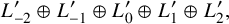 $$ \begin{align} L^{\prime}_{-2}\oplus L^{\prime}_{-1}\oplus L^{\prime}_0\oplus L^{\prime}_1\oplus L^{\prime}_2, \end{align} $$
with $L^{\prime }_{-2}=\langle c \rangle $
and
$L^{\prime }_{-2}=\langle c \rangle $
and $L^{\prime }_2 = \langle d \rangle $
.
$L^{\prime }_2 = \langle d \rangle $
.
Now set
 $$\begin{align*}V := L_{-1}\cap L^{\prime}_{-1}, \quad X := L_{-1}\cap L^{\prime}_0, \quad V':=L_{-1}\cap L^{\prime}_1, \quad X' := L_0 \cap L^{\prime}_{-1}. \end{align*}$$
Lemma 5.5. We have $c,d \in L_0$
and
$c,d \in L_0$
and $x,y \in L^{\prime }_0$
.
$x,y \in L^{\prime }_0$
.
Proof. Since $(x,c),(c,y) \in E_0$
, it follows immediately from Proposition 2.5 that
$(x,c),(c,y) \in E_0$
, it follows immediately from Proposition 2.5 that $c\in L_0$
. The proof of the other three statements is similar.
$c\in L_0$
. The proof of the other three statements is similar.
Lemma 5.6. We have $g_c(L_{-2}\oplus L_{-1}\oplus L_1\oplus L_2)=0$
and
$g_c(L_{-2}\oplus L_{-1}\oplus L_1\oplus L_2)=0$
and $g_d(L_{-2}\oplus L_{-1}\oplus L_1\oplus L_2) = 0$
.
$g_d(L_{-2}\oplus L_{-1}\oplus L_1\oplus L_2) = 0$
.
Proof. We show the claim for $g_c$
. Since
$g_c$
. Since $(c,x),(c,y) \in E_0$
, we get
$(c,x),(c,y) \in E_0$
, we get $g_c(x)=0$
and
$g_c(x)=0$
and $g_c(y)=0$
. Next, let
$g_c(y)=0$
. Next, let $l\in L_{-1}$
be arbitrary and recall from Proposition 2.4(iii) that
$l\in L_{-1}$
be arbitrary and recall from Proposition 2.4(iii) that $[x,[y,l]]=-l$
. Using the associativity of g, we get
$[x,[y,l]]=-l$
. Using the associativity of g, we get
 $$\begin{align*}-g_c(l)=g(c,[x,[y,l]])=g([c,x],[y,l])=g(0,[y,l])=0,\end{align*}$$
so $g_c(L_{-1}) = 0$
. Similarly,
$g_c(L_{-1}) = 0$
. Similarly, $g_c(L_{1}) = 0$
.
$g_c(L_{1}) = 0$
.
Proposition 5.7. We have decompositions
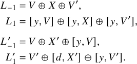 $$ \begin{align*} L_{-1} &= V \oplus X \oplus V' , \\ L_{1} &= [y,V] \oplus [y,X] \oplus [y,V'], \\[1ex] L^{\prime}_{-1} &= V \oplus X' \oplus [y,V] , \\ L^{\prime}_{1} &= V' \oplus [d,X'] \oplus [y,V']. \end{align*} $$
Proof. By Lemma 5.6, we get $g_d(L_{-1})=0$
and hence
$g_d(L_{-1})=0$
and hence $L_{-1} \leq L^{\prime }_{\geq -1}$
by Proposition 2.4(v) applied to the grading (55). Similarly, it follows from
$L_{-1} \leq L^{\prime }_{\geq -1}$
by Proposition 2.4(v) applied to the grading (55). Similarly, it follows from $g_c(L_{-1})=0$
that
$g_c(L_{-1})=0$
that $L_{-1} \leq L^{\prime }_{\leq 1}$
. Hence,
$L_{-1} \leq L^{\prime }_{\leq 1}$
. Hence, $L_{-1} \leq L^{\prime }_{-1}\oplus L^{\prime }_0\oplus L^{\prime }_1$
.
$L_{-1} \leq L^{\prime }_{-1}\oplus L^{\prime }_0\oplus L^{\prime }_1$
.
The rest of the proof of the decomposition of $L_{-1}$
now follows exactly the same method as in the proof of Proposition 4.6, using the grading element
$L_{-1}$
now follows exactly the same method as in the proof of Proposition 4.6, using the grading element $[c,d]\in L_0$
, so we can safely omit the details. The second decomposition follows from the first by applying the isomorphism
$[c,d]\in L_0$
, so we can safely omit the details. The second decomposition follows from the first by applying the isomorphism $\operatorname {\mathrm {ad}}_y$
from
$\operatorname {\mathrm {ad}}_y$
from $L_{-1}$
to
$L_{-1}$
to $L_1$
; see Proposition 2.4(iii).
$L_1$
; see Proposition 2.4(iii).
The other two decompositions follow in a similar fashion by interchanging the roles of the two gradings (54) and (55).
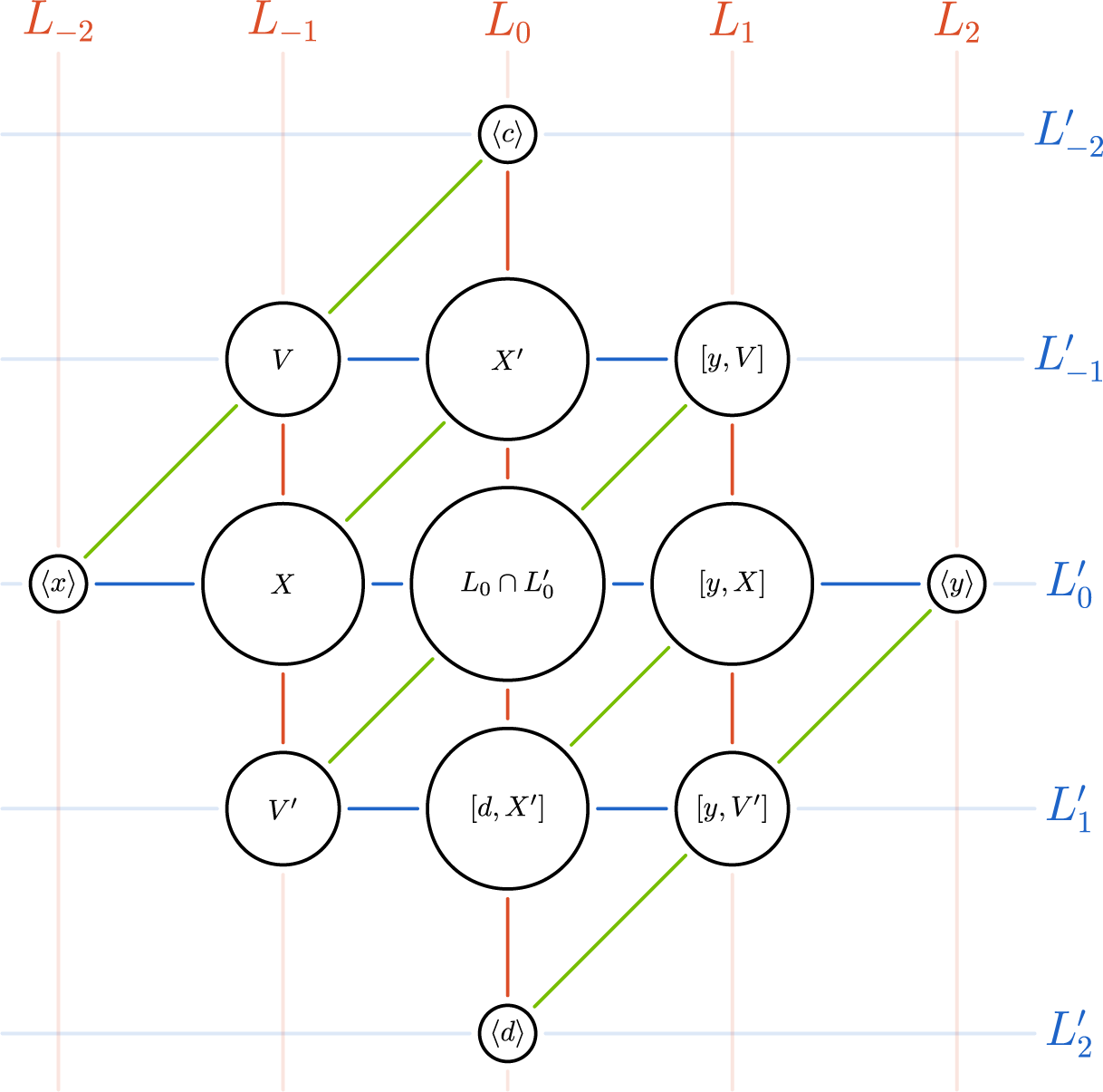
Figure 2 Intersecting gradings for quadrangular algebras.
We have summarized all the information about the intersections of the two gradings in Figure 2. Notice that the four subspaces V, $V' = [d,V]$
,
$V' = [d,V]$
, $[y,V]$
and
$[y,V]$
and $[y,V'] = [y,[d,V]]$
are all isomorphic, by Proposition 2.4(iii). (See also the proof of Corollary 5.8 below.) For the same reason,
$[y,V'] = [y,[d,V]]$
are all isomorphic, by Proposition 2.4(iii). (See also the proof of Corollary 5.8 below.) For the same reason, $X \cong [y,X]$
and
$X \cong [y,X]$
and $X' \cong [d,X']$
. We will see later that also the subspaces X and
$X' \cong [d,X']$
. We will see later that also the subspaces X and $X'$
are isomorphic; see Corollary 5.24. Notice that in Figure 2, we have also identified a third grading (diagonally), but this grading is not directly necessary for our purposes. See, however, Remark 5.60 below.
$X'$
are isomorphic; see Corollary 5.24. Notice that in Figure 2, we have also identified a third grading (diagonally), but this grading is not directly necessary for our purposes. See, however, Remark 5.60 below.
By combining both gradings, we already obtain some more information on the Lie bracket.
Corollary 5.8. The following identities and inclusions hold:
 $$ \begin{align} &[c,V']=V, && [d,V]=V', \end{align} $$
 $$ \begin{align} &[c,V]=0, && [d,V']=0, \end{align} $$
 $$ \begin{align} &[c,X]=0, && [d,X]=0, \end{align} $$
 $$ \begin{align} &[V,V]=0, \quad [V',V']=0, \quad && [V,X]=0, \quad [V',X]=0, \end{align} $$
 $$ \begin{align} &[X,[X,[y,V]]\leq V, && [X,[X,[y,V']]\leq V', \end{align} $$
 $$ \begin{align} &[X,[V,[y,V']]]\leq X, && [X,[V',[y,V]]]\leq X. \end{align} $$
Proof. By Proposition 2.4(iii) applied on the grading (55), the map $\operatorname {\mathrm {ad}}_d$
is an isomorphism from
$\operatorname {\mathrm {ad}}_d$
is an isomorphism from $L^{\prime }_{-1}$
to
$L^{\prime }_{-1}$
to $L^{\prime }_1$
with inverse
$L^{\prime }_1$
with inverse $-\operatorname {\mathrm {ad}}_c$
. Since
$-\operatorname {\mathrm {ad}}_c$
. Since $c,d \in L_0$
, these maps preserve the grading (54). It follows from Proposition 5.7 that
$c,d \in L_0$
, these maps preserve the grading (54). It follows from Proposition 5.7 that $\operatorname {\mathrm {ad}}_d$
induces an isomorphism from V to
$\operatorname {\mathrm {ad}}_d$
induces an isomorphism from V to $V'$
, with inverse
$V'$
, with inverse $-\operatorname {\mathrm {ad}}_c$
. This shows (56).
$-\operatorname {\mathrm {ad}}_c$
. This shows (56).
The relations (57) to (61) all follow immediately from combining the two gradings, as can be seen from Figure 2.
We will now exploit the uniqueness of certain extremal elements to define a quadratic form on the vector space V.
Lemma 5.9. For every $v \in V$
, there is a unique
$v \in V$
, there is a unique $\lambda \in k$
such that
$\lambda \in k$
such that
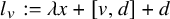 $$ \begin{align} l_v := \lambda x + [v,d] + d \end{align} $$
is an extremal element. Moreover, $l_v=l_{v'}$
if and only if
$l_v=l_{v'}$
if and only if $v=v'$
, where
$v=v'$
, where $v,v'\in V$
.
$v,v'\in V$
.
Proof. Since $v \in L_{-1}$
, Theorem 3.16 implies that there exists a v-exponential automorphism
$v \in L_{-1}$
, Theorem 3.16 implies that there exists a v-exponential automorphism $\alpha \in \operatorname {\mathrm {Aut}}(L)$
. Then
$\alpha \in \operatorname {\mathrm {Aut}}(L)$
. Then $\alpha (d)$
is an extremal element, and we have
$\alpha (d)$
is an extremal element, and we have $\alpha (d) = q_\alpha (d) + [v,d] + d$
with
$\alpha (d) = q_\alpha (d) + [v,d] + d$
with $q_\alpha (d) \in L_{-2} = \langle x \rangle $
, showing the existence.
$q_\alpha (d) \in L_{-2} = \langle x \rangle $
, showing the existence.
Assume now that that there are two distinct scalars such that (62) holds. Then the $2$
-dimensional subspace
$2$
-dimensional subspace $\langle x, [v,d] + d \rangle $
contains three distinct extremal elements, so Proposition 1.8 implies that this is a line of the extremal geometry. This contradicts Corollary 2.6.
$\langle x, [v,d] + d \rangle $
contains three distinct extremal elements, so Proposition 1.8 implies that this is a line of the extremal geometry. This contradicts Corollary 2.6.
Finally, if $l_v = l_{v'}$
for certain
$l_v = l_{v'}$
for certain $v,v' \in V$
, then
$v,v' \in V$
, then $[v,d]=[v',d]$
. Proposition 2.4(iii) applied on the grading (55) then implies that
$[v,d]=[v',d]$
. Proposition 2.4(iii) applied on the grading (55) then implies that $v = v'$
.
$v = v'$
.
Definition 5.10. Define the map $Q \colon V \to k$
by setting
$Q \colon V \to k$
by setting $Q(v)$
to be the unique
$Q(v)$
to be the unique $\lambda \in k$
from Lemma 5.9 – that is, such that the element
$\lambda \in k$
from Lemma 5.9 – that is, such that the element
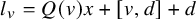 $$ \begin{align} l_v = Q(v)x + [v,d] + d \end{align} $$
is an extremal element. Define the bilinear form $T \colon V\times V \to k$
by
$T \colon V\times V \to k$
by
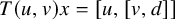 $$\begin{align*}T(u,v) x = [u,[v,d]] \end{align*}$$
for all $u,v \in V$
.
$u,v \in V$
.
Remark 5.11. The uniqueness aspect, although easy to prove, is somewhat subtle, because the v-exponential automorphism $\alpha $
that we have used in the proof of Lemma 5.9 is not unique. Notice, however, that we will be able to single out a unique v-exponential automorphism in Definition 5.15 below.
$\alpha $
that we have used in the proof of Lemma 5.9 is not unique. Notice, however, that we will be able to single out a unique v-exponential automorphism in Definition 5.15 below.
Lemma 5.12. The map Q is a quadratic form on V, with corresponding bilinear form T.
Proof. Let $\lambda \in k$
and
$\lambda \in k$
and $u,v \in V$
. Let
$u,v \in V$
. Let $\alpha ,\beta $
be a u-exponential and a v-exponential automorphism, respectively. Then
$\alpha ,\beta $
be a u-exponential and a v-exponential automorphism, respectively. Then $q_{\alpha }(d) + [u,d] + d \in E$
and
$q_{\alpha }(d) + [u,d] + d \in E$
and $q_\alpha (d) = Q(u)x$
. By Theorem 3.13(vii),
$q_\alpha (d) = Q(u)x$
. By Theorem 3.13(vii), $\lambda ^2 q_{\alpha }(d) + \lambda [u,d] + d \in E$
. Hence,
$\lambda ^2 q_{\alpha }(d) + \lambda [u,d] + d \in E$
. Hence, $Q(\lambda u)=\lambda ^2 Q(u)$
.
$Q(\lambda u)=\lambda ^2 Q(u)$
.
Next, we have
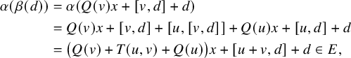 $$ \begin{align*} \alpha(\beta(d)) &= \alpha( Q(v)x + [v,d] + d) \\ &= Q(v)x + [v,d] + [u,[v,d]] + Q(u)x + [u,d] + d \\ &= \big( Q(v) + T(u,v) + Q(u) \big) x + [u+v, d] + d \in E, \end{align*} $$
and hence, $Q(u+v) = Q(v) + T(u,v) + Q(u)$
. The map T is bilinear by construction; hence, Q is a quadratic form on V with corresponding bilinear form T.
$Q(u+v) = Q(v) + T(u,v) + Q(u)$
. The map T is bilinear by construction; hence, Q is a quadratic form on V with corresponding bilinear form T.
We will see in Lemma 5.19 below that Q is not the zero map. The following lemma is a first step, useful in its own right.
Lemma 5.13. Let $v \in V \setminus \{ 0 \}$
be such that
$v \in V \setminus \{ 0 \}$
be such that $Q(v) = 0$
. Then v,
$Q(v) = 0$
. Then v, $[v,d]$
,
$[v,d]$
, $[y,v]$
and
$[y,v]$
and $[y,[v,d]]$
are extremal elements.
$[y,[v,d]]$
are extremal elements.
Proof. By definition of Q and Lemma 5.12, we have $\lambda [v,d] + d \in E$
for all
$\lambda [v,d] + d \in E$
for all $\lambda \in k$
. Note that
$\lambda \in k$
. Note that $[v,d] \neq 0$
since
$[v,d] \neq 0$
since $\operatorname {\mathrm {ad}}_d$
induces an isomorphism from V to
$\operatorname {\mathrm {ad}}_d$
induces an isomorphism from V to $V'$
. By Proposition 1.8, this implies that
$V'$
. By Proposition 1.8, this implies that $[v,d]\in E$
. Since
$[v,d]\in E$
. Since $\operatorname {\mathrm {ad}}_c$
maps extremal elements in
$\operatorname {\mathrm {ad}}_c$
maps extremal elements in $L^{\prime }_1$
to extremal elements in
$L^{\prime }_1$
to extremal elements in $L^{\prime }_{-1}$
(by Lemma 2.8), it follows that also
$L^{\prime }_{-1}$
(by Lemma 2.8), it follows that also $v = [c, [v,d]] \in E$
. Similarly,
$v = [c, [v,d]] \in E$
. Similarly, $\operatorname {\mathrm {ad}}_y$
maps extremal elements in
$\operatorname {\mathrm {ad}}_y$
maps extremal elements in $L_{-1}$
to extremal elements in
$L_{-1}$
to extremal elements in $L_1$
, and thus also
$L_1$
, and thus also $[y,v]$
and
$[y,v]$
and $[y, [v,d]]$
are extremal elements.
$[y, [v,d]]$
are extremal elements.
Lemma 5.14. Let $v \in V$
. Then
$v \in V$
. Then
 $$ \begin{align} &Q(v)x + v + c \in E, && x + v + Q(v)c \in E, \end{align} $$
 $$ \begin{align} &Q(v)x + [v,d] + d \in E, && x + [v,d] + Q(v)d \in E, \end{align} $$
 $$ \begin{align} &Q(v)y + [y,v] + c \in E, && y + [y,v] + Q(v)c \in E, \end{align} $$
 $$ \begin{align} &Q(v)y + [y,[v,d]] + d \in E, && y + [y,[v,d]] + Q(v)d \in E. \end{align} $$
Moreover, in each case, $Q(v)$
is the unique scalar that makes the statement true.
$Q(v)$
is the unique scalar that makes the statement true.
Proof. Assume first that $Q(v) = 0$
. Then by Lemma 5.13, we have
$Q(v) = 0$
. Then by Lemma 5.13, we have $v \in E$
. By Corollary 2.6, this element is collinear with c and with x, so in particular,
$v \in E$
. By Corollary 2.6, this element is collinear with c and with x, so in particular, $v + c \in E$
and
$v + c \in E$
and $x + v \in E$
. The proof of the other 6 statements is similar.
$x + v \in E$
. The proof of the other 6 statements is similar.
Assume now that $Q(v) \neq 0$
. By definition,
$Q(v) \neq 0$
. By definition, $Q(v)x + [v,d] + d \in E$
. By replacing v with
$Q(v)x + [v,d] + d \in E$
. By replacing v with $Q(v)^{-1} v$
, we also get
$Q(v)^{-1} v$
, we also get $Q(v)^{-1}x + Q(v)^{-1} [v,d] + d \in E$
, and multiplying by
$Q(v)^{-1}x + Q(v)^{-1} [v,d] + d \in E$
, and multiplying by $Q(v)$
now gives
$Q(v)$
now gives $x + [v,d] + Q(v) d \in E$
. This proves (65).
$x + [v,d] + Q(v) d \in E$
. This proves (65).
Next, let $\varphi \in \operatorname {\mathrm {Aut}}(L)$
be the automorphism obtained from Lemma 2.8 applied to the grading (55). In particular,
$\varphi \in \operatorname {\mathrm {Aut}}(L)$
be the automorphism obtained from Lemma 2.8 applied to the grading (55). In particular, $\varphi (d) = c$
and
$\varphi (d) = c$
and $\varphi (x) = x + [c, [d, x]] = x$
, so we get
$\varphi (x) = x + [c, [d, x]] = x$
, so we get
 $$\begin{align*}\varphi \big( Q(v)x+[v,d]+d \big) = Q(v)x+[c,[v,d]]+c = Q(v)x+v+c \in E. \end{align*}$$
We can again replace v by $Q(v)^{-1} v$
to get
$Q(v)^{-1} v$
to get $x + v + Q(v)c \in E$
as well. This proves (64).
$x + v + Q(v)c \in E$
as well. This proves (64).
We now apply the automorphism $\psi \in \operatorname {\mathrm {Aut}}(L)$
obtained from Lemma 2.8 applied to the grading (54). Then in exactly the same way as in the previous paragraph, applying
$\psi \in \operatorname {\mathrm {Aut}}(L)$
obtained from Lemma 2.8 applied to the grading (54). Then in exactly the same way as in the previous paragraph, applying $\psi $
on (64) yields (66) and applying
$\psi $
on (64) yields (66) and applying $\psi $
on (65) yields (67).
$\psi $
on (65) yields (67).
Finally, the uniqueness statement follows in each case in exactly the same way as in the proof of Lemma 5.9.
The previous lemma will, in particular, allow us to single out a specific v-exponential automorphism, as announced in Remark 5.11 above.
Definition 5.15. Let $v \in V$
. Then by Lemma 5.14 applied on
$v \in V$
. Then by Lemma 5.14 applied on $-v$
, we have
$-v$
, we have $y + [v,y] + Q(v)c \in E$
. By Proposition 3.22, there exists a unique automorphism
$y + [v,y] + Q(v)c \in E$
. By Proposition 3.22, there exists a unique automorphism $\alpha _v \in E_-(x,y)$
such that
$\alpha _v \in E_-(x,y)$
such that
 $$ \begin{align} \alpha_v(y) = y + [v,y] + Q(v)c. \end{align} $$
By Theorem 3.13(vi), $\alpha _v$
is an
$\alpha _v$
is an $\ell $
-exponential automorphism for some
$\ell $
-exponential automorphism for some $\ell \in L_{-1}$
, but then
$\ell \in L_{-1}$
, but then $[\ell , y] = [v,y]$
, and therefore, by applying
$[\ell , y] = [v,y]$
, and therefore, by applying $\operatorname {\mathrm {ad}}_x$
, we get
$\operatorname {\mathrm {ad}}_x$
, we get $\ell = v$
, so
$\ell = v$
, so $\alpha _v$
is a v-exponential automorphism. Notice that by Lemma 5.9 and Definition 5.10, we also have
$\alpha _v$
is a v-exponential automorphism. Notice that by Lemma 5.9 and Definition 5.10, we also have
 $$ \begin{align} \alpha_v(d) = d + [v,d] + Q(v)x. \end{align} $$
In a similar way, we can define a unique $[y,v]$
-exponential automorphism for each
$[y,v]$
-exponential automorphism for each $v \in V$
, this time with respect to the
$v \in V$
, this time with respect to the $L_i'$
-grading (55). We will need these automorphisms in Lemma 5.53 and Proposition 5.55 below.
$L_i'$
-grading (55). We will need these automorphisms in Lemma 5.53 and Proposition 5.55 below.
Definition 5.16. Let $v \in V$
and consider
$v \in V$
and consider $[y,v] \in [y,V]$
. By Lemma 5.14, we have
$[y,v] \in [y,V]$
. By Lemma 5.14, we have $d + [y, [v,d]] + Q(v)y \in E$
. By Proposition 3.22, there exists a unique automorphism
$d + [y, [v,d]] + Q(v)y \in E$
. By Proposition 3.22, there exists a unique automorphism $\beta _v \in E_-(c,d)$
such that
$\beta _v \in E_-(c,d)$
such that
 $$\begin{align*}\beta_v(d) = d + [y, [v,d]] + Q(v)y = d + [[y,v], d] + Q(v)y. \end{align*}$$
In particular, by Theorem 3.13(vi), $\beta _v$
is an
$\beta _v$
is an $\ell $
-exponential automorphism for some
$\ell $
-exponential automorphism for some $\ell \in L^{\prime }_{-1}$
, but then
$\ell \in L^{\prime }_{-1}$
, but then $[\ell , d] = [[y,v], d]$
, so by applying
$[\ell , d] = [[y,v], d]$
, so by applying $\operatorname {\mathrm {ad}}_c$
, we get
$\operatorname {\mathrm {ad}}_c$
, we get $\ell = [y,v]$
, so
$\ell = [y,v]$
, so $\beta _v$
is a
$\beta _v$
is a $[y,v]$
-exponential automorphism with respect to the
$[y,v]$
-exponential automorphism with respect to the $L_i'$
-grading (55). Notice that
$L_i'$
-grading (55). Notice that $\beta _v(x) = x + [[y,v], x] + \lambda c \in E$
for some
$\beta _v(x) = x + [[y,v], x] + \lambda c \in E$
for some $\lambda \in k$
, so
$\lambda \in k$
, so $x + v + \lambda c \in E$
, and hence by the uniqueness part of Lemma 5.14, we have
$x + v + \lambda c \in E$
, and hence by the uniqueness part of Lemma 5.14, we have
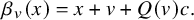 $$\begin{align*}\beta_v(x) = x + v + Q(v) c. \end{align*}$$
It is a slightly subtle fact that $\alpha _v$
is not only v-exponential with respect to the
$\alpha _v$
is not only v-exponential with respect to the $L_i$
-grading (54), but also with respect to the
$L_i$
-grading (54), but also with respect to the $L^{\prime }_i$
-grading (55), as we now show.
$L^{\prime }_i$
-grading (55), as we now show.
Proposition 5.17. Let $v \in V = L_{-1} \cap L^{\prime }_{-1}$
. Then
$v \in V = L_{-1} \cap L^{\prime }_{-1}$
. Then $\alpha _v$
is also v-exponential with respect to the
$\alpha _v$
is also v-exponential with respect to the $L^{\prime }_i$
-grading (55).
$L^{\prime }_i$
-grading (55).
Proof. First apply Assumption 5.1(i) and extend k to a larger field $k'$
such that the extremal geometry
$k'$
such that the extremal geometry $E(L \otimes k')$
contains lines. Let
$E(L \otimes k')$
contains lines. Let $\alpha _v$
be the v-exponential automorphism with respect to the
$\alpha _v$
be the v-exponential automorphism with respect to the $L_i$
-grading (54) as in Definition 5.15. Moreover, let
$L_i$
-grading (54) as in Definition 5.15. Moreover, let $\alpha ^{\prime }_v$
be the unique v-exponential automorphism with respect to the
$\alpha ^{\prime }_v$
be the unique v-exponential automorphism with respect to the $L^{\prime }_i$
-grading (55) such that
$L^{\prime }_i$
-grading (55) such that
 $$\begin{align*}\alpha^{\prime}_v(d) = d + [v,d] + Q(v)x , \end{align*}$$
similarly to what we have done in Definition 5.16, and notice that also
 $$\begin{align*}\alpha^{\prime}_v(y) = y + [v,y] + Q(v)c = \alpha_v(y). \end{align*}$$
We claim that $\alpha _v$
and
$\alpha _v$
and $\alpha ^{\prime }_v$
also coincide on
$\alpha ^{\prime }_v$
also coincide on $L_{-1} = V \oplus X \oplus V'$
; it will then follow from Lemma 3.3 that
$L_{-1} = V \oplus X \oplus V'$
; it will then follow from Lemma 3.3 that $\alpha _v = \alpha ^{\prime }_v$
. Our claim is obvious by the grading for elements of
$\alpha _v = \alpha ^{\prime }_v$
. Our claim is obvious by the grading for elements of $V \oplus X$
, so it only remains to show that
$V \oplus X$
, so it only remains to show that $\alpha _v([d,w]) = \alpha ^{\prime }_v([d,w])$
for all
$\alpha _v([d,w]) = \alpha ^{\prime }_v([d,w])$
for all $w \in V$
. This is also clear, however, because
$w \in V$
. This is also clear, however, because $\alpha _v$
and
$\alpha _v$
and $\alpha ^{\prime }_v$
coincide on both
$\alpha ^{\prime }_v$
coincide on both $\langle d \rangle $
and V.
$\langle d \rangle $
and V.
We conclude that indeed, $\alpha _v = \alpha ^{\prime }_v$
, so in particular,
$\alpha _v = \alpha ^{\prime }_v$
, so in particular, $\alpha _v$
is also v-exponential with respect to the
$\alpha _v$
is also v-exponential with respect to the $L^{\prime }_i$
-grading (55).
$L^{\prime }_i$
-grading (55).
Lemma 5.18. We have $V \neq 0$
and
$V \neq 0$
and $V' \neq 0$
. Moreover, the bilinear form
$V' \neq 0$
. Moreover, the bilinear form $T \colon V \times V \to k$
is nondegenerate.
$T \colon V \times V \to k$
is nondegenerate.
Proof. Notice that by (56), we have $V \neq 0$
if and only if
$V \neq 0$
if and only if $V' \neq 0$
. Suppose now that
$V' \neq 0$
. Suppose now that $V = V' = 0$
; then
$V = V' = 0$
; then $L_{-1} = X$
and
$L_{-1} = X$
and $L_1 = [y, X]$
(see Figure 2), so
$L_1 = [y, X]$
(see Figure 2), so
 $$\begin{align*}L_{-2} \oplus L_{-1} \oplus L_1 \oplus L_2 \leq L^{\prime}_0. \end{align*}$$
In particular, by Proposition 2.4(ii), $\operatorname {\mathrm {ad}}_{[c,d]}$
maps
$\operatorname {\mathrm {ad}}_{[c,d]}$
maps $L_{-2} \oplus L_{-1} \oplus L_1 \oplus L_2$
to
$L_{-2} \oplus L_{-1} \oplus L_1 \oplus L_2$
to $0$
. Since L is generated by
$0$
. Since L is generated by $L_{-2} \oplus L_{-1} \oplus L_1 \oplus L_2$
, this implies that the map
$L_{-2} \oplus L_{-1} \oplus L_1 \oplus L_2$
, this implies that the map $\operatorname {\mathrm {ad}}_{[c,d]}$
is zero on all of L, a contradiction. Hence,
$\operatorname {\mathrm {ad}}_{[c,d]}$
is zero on all of L, a contradiction. Hence, $V \neq 0$
and
$V \neq 0$
and $V' \neq 0$
.
$V' \neq 0$
.
Now let $v \in V \setminus \{ 0 \}$
be arbitrary, and assume that
$v \in V \setminus \{ 0 \}$
be arbitrary, and assume that $T(v,u) = 0$
for all
$T(v,u) = 0$
for all $u \in V$
. Then by definition of T, this implies that
$u \in V$
. Then by definition of T, this implies that $[v, V'] = 0$
, but since also
$[v, V'] = 0$
, but since also $[v, X] = 0$
and
$[v, X] = 0$
and $[v, V] = 0$
by the grading, we then have
$[v, V] = 0$
by the grading, we then have $[v, L_{-1}] = 0$
. This contradicts Lemma 2.11.
$[v, L_{-1}] = 0$
. This contradicts Lemma 2.11.
Lemma 5.19. There exists $v\in V$
such that
$v\in V$
such that $Q(v)\neq 0$
.
$Q(v)\neq 0$
.
Proof. Assume that $Q(v) = 0$
for all
$Q(v) = 0$
for all $v \in V$
. By Lemma 5.13, there exist elements in
$v \in V$
. By Lemma 5.13, there exist elements in $E \cap L_{-1}$
, so by Corollary 2.6, the extremal geometry contains lines. In fact, each nonzero
$E \cap L_{-1}$
, so by Corollary 2.6, the extremal geometry contains lines. In fact, each nonzero $v \in V$
is an extremal element collinear with x and, by Lemma 5.14, also collinear with c. Moreover, it now follows from the grading and Corollary 2.6 that
$v \in V$
is an extremal element collinear with x and, by Lemma 5.14, also collinear with c. Moreover, it now follows from the grading and Corollary 2.6 that $E_{-1}(x) \cap E_{-1}(c) = V \setminus \{ 0 \}$
.
$E_{-1}(x) \cap E_{-1}(c) = V \setminus \{ 0 \}$
.
By Proposition 3.5, however, there is a (unique) symplecton S containing $\langle x \rangle $
and
$\langle x \rangle $
and $\langle c \rangle $
. By Proposition 3.5(i), S is a nondegenerate polar space of rank
$\langle c \rangle $
. By Proposition 3.5(i), S is a nondegenerate polar space of rank $\geq 2$
, so we can find two distinct non-collinear points
$\geq 2$
, so we can find two distinct non-collinear points $\langle u \rangle $
and
$\langle u \rangle $
and $\langle v \rangle $
both collinear to both
$\langle v \rangle $
both collinear to both $\langle x \rangle $
and
$\langle x \rangle $
and $\langle c \rangle $
. By the previous paragraph, u and v belong to
$\langle c \rangle $
. By the previous paragraph, u and v belong to $V \setminus \{ 0 \}$
. However, this implies that also
$V \setminus \{ 0 \}$
. However, this implies that also $u+v \in V \setminus \{ 0 \}$
, so by assumption,
$u+v \in V \setminus \{ 0 \}$
, so by assumption, $Q(u+v) = 0$
, so also
$Q(u+v) = 0$
, so also $u+v$
is an extremal element. This contradicts Proposition 1.8 because u and v are not collinear.
$u+v$
is an extremal element. This contradicts Proposition 1.8 because u and v are not collinear.
In a similar way as in Lemma 4.18, we can now ensure that Q has a base point (i.e., $Q(v) = 1$
for some
$Q(v) = 1$
for some $v \in V$
).
$v \in V$
).
Lemma 5.20. We can re-choose x in y in Notation 5.4 in such a way that $Q(e) = 1$
for some
$Q(e) = 1$
for some $e \in V$
. We call e a base point for Q.
$e \in V$
. We call e a base point for Q.
Proof. Consider $e \in V$
such that
$e \in V$
such that $Q(e) \neq 0$
. Set
$Q(e) \neq 0$
. Set $\tilde x := Q(e)x$
and
$\tilde x := Q(e)x$
and $\tilde y := Q(e)^{-1}y$
. Then
$\tilde y := Q(e)^{-1}y$
. Then $\tilde x$
,
$\tilde x$
, $\tilde y$
, c and d still satisfy the conclusions from Proposition 5.3. Since we have only replaced these elements by a scalar multiple, this does not affect any of the decompositions.
$\tilde y$
, c and d still satisfy the conclusions from Proposition 5.3. Since we have only replaced these elements by a scalar multiple, this does not affect any of the decompositions.
Now denote the map obtained as in Definition 5.10 from these new choices by $\tilde Q$
. Since
$\tilde Q$
. Since $\tilde x + [e,d] + d = Q(e)x + [e,d] + d \in E$
, it follows that indeed
$\tilde x + [e,d] + d = Q(e)x + [e,d] + d \in E$
, it follows that indeed $\tilde Q(e) = 1$
.
$\tilde Q(e) = 1$
.
Definition 5.21. Assume from now on that $e \in V$
is a base point for Q.
$e \in V$
is a base point for Q.
-
(i) We set
$$\begin{align*}e' := [d,e] \in V', \quad f := [y,e] \in [y,V], \quad f' := [y, e'] \in [y, V']. \end{align*}$$
Notice that
$f' = [d,f]$
because
$[d,y] = 0$
. -
(ii) Since T is nondegenerate by Lemma 5.18, we can fix an element
$\delta \in V$
such that
$T(e, \delta ) = 1$
. If
$\operatorname {\mathrm {char}}(k) \neq 2$
, we will assume that
$\delta = \tfrac {1}{2} e$
.We may assume, in addition, that
$Q(\delta ) \neq 0$
. Indeed, this holds automatically if
$\operatorname {\mathrm {char}}(k) \neq 2$
, and if
$\operatorname {\mathrm {char}}(k) = 2$
and
$Q(\delta ) = 0$
, then we choose some
$\lambda \in k$
with
$\lambda ^2 \neq \lambda $
(which exist because we assume
$|k|> 2$
; see Assumption 5.1) and we replace
$\delta $
by
$\lambda e + \delta $
.


Remark 5.22. This definition of $\delta $
corresponds to the definition of
$\delta $
corresponds to the definition of $\delta $
for quadrangular algebras in [Reference WeissWei06, Definition 4.1] and [Reference Mühlherr and WeissMW19, Definition 7.1]. In fact, we will use this
$\delta $
for quadrangular algebras in [Reference WeissWei06, Definition 4.1] and [Reference Mühlherr and WeissMW19, Definition 7.1]. In fact, we will use this $\delta $
in Proposition 5.28 below to ensure that our quadrangular algebra will be
$\delta $
in Proposition 5.28 below to ensure that our quadrangular algebra will be $\delta $
-standard; see Definition 5.29(iii).
$\delta $
-standard; see Definition 5.29(iii).
Lemma 5.23. For any $v\in V$
, we have
$v\in V$
, we have
 $$ \begin{align} Q(v) \big( [c,d] - [x,y] \big) &= [[v,d],[v,y]]; \end{align} $$
 $$ \begin{align} Q(v) \big( [c,d] + [x,y] \big) &= [v,[y,[d,v]]]. \end{align} $$
In particular,
 $$ \begin{align} [e', f] = [c,d] - [x,y] \quad \text{and} \quad [e, f'] = [c,d] + [x,y]. \end{align} $$
Proof. Let $v \in V$
and let
$v \in V$
and let $\alpha _v \in \operatorname {\mathrm {Aut}}(L)$
be as in Definition 5.15. Since
$\alpha _v \in \operatorname {\mathrm {Aut}}(L)$
be as in Definition 5.15. Since $[d,y] = 0$
and
$[d,y] = 0$
and $\alpha _v \in \operatorname {\mathrm {Aut}}(L)$
, we also get
$\alpha _v \in \operatorname {\mathrm {Aut}}(L)$
, we also get $[\alpha _v(d), \alpha _v(y)] = 0$
, so by (68) and (69), we get
$[\alpha _v(d), \alpha _v(y)] = 0$
, so by (68) and (69), we get
 $$\begin{align*}\big[ d + [v,d] + Q(v)x, \ y + [v,y] + Q(v)c \big] = 0. \end{align*}$$
Expanding this – or in fact, only expanding the $(L_0 \cap L^{\prime }_0)$
-component suffices – yields (70).
$(L_0 \cap L^{\prime }_0)$
-component suffices – yields (70).
Next, observe that $[v,[v,d]]=T(v,v)x=2Q(v)x$
by Lemma 5.12. Hence,
$[v,[v,d]]=T(v,v)x=2Q(v)x$
by Lemma 5.12. Hence,
 $$\begin{align*}[[v,d],[v,y]] = [v,[[v,d],y]] - 2Q(v)[x,y] , \end{align*}$$
so together with (70), this yields (71).
Finally, (72) now follows by plugging in $v=e$
and using
$v=e$
and using $Q(e)=1$
.
$Q(e)=1$
.
Corollary 5.24. The restriction of $\operatorname {\mathrm {ad}}_f$
to X defines a linear isomorphism from X to
$\operatorname {\mathrm {ad}}_f$
to X defines a linear isomorphism from X to $X'$
with inverse
$X'$
with inverse $\operatorname {\mathrm {ad}}_{e'}$
.
$\operatorname {\mathrm {ad}}_{e'}$
.
Proof. Let $a \in X$
and
$a \in X$
and $a' \in X'$
. Then using (72) and Proposition 2.4(ii), we get
$a' \in X'$
. Then using (72) and Proposition 2.4(ii), we get
 $$ \begin{align*} [e', [f,a]] &= [a, [f, e']] = [[c,d] - [x,y], a] = a, \\ [f, [e',a']] &= [a', [e', f]] = [-[c,d] + [x,y], a'] = a'. \end{align*} $$
We can now also determine the Lie bracket between V and $[y,V]$
explicitly.
$[y,V]$
explicitly.
Proposition 5.25. Let $v,w \in V$
. Then
$v,w \in V$
. Then $[[y,v], w] = T(v,w)c$
.
$[[y,v], w] = T(v,w)c$
.
Proof. Since $V = L_{-1} \cap L^{\prime }_{-1}$
, it follows from Proposition 2.4(ii) that
$V = L_{-1} \cap L^{\prime }_{-1}$
, it follows from Proposition 2.4(ii) that
 $$\begin{align*}[[c,d] - [x,y], w] = 0. \end{align*}$$
By (70), therefore, we have $\big [ [[v,d], [v,y]], \, w \big ] = 0$
, and hence,
$\big [ [[v,d], [v,y]], \, w \big ] = 0$
, and hence,
 $$\begin{align*}\big[ [v,d], \, [[v,y], w] \big] = \big[ [v,y], \, [[v,d], w] \big]. \end{align*}$$
By the grading, we know that $[[y,v], w] = \mu c$
for some
$[[y,v], w] = \mu c$
for some $\mu \in k$
. Hence, by Definition 5.10, the previous equality reduces to
$\mu \in k$
. Hence, by Definition 5.10, the previous equality reduces to
 $$\begin{align*}[[v,d], -\mu c] = [[v,y], -T(v,w)x]. \end{align*}$$
By Proposition 2.4(iii), this can be rewritten as $\mu v = T(v,w)v$
, so
$\mu v = T(v,w)v$
, so $\mu = T(v,w)$
.
$\mu = T(v,w)$
.
Definition 5.26. We define maps $h \colon X\times X\to V$
and
$h \colon X\times X\to V$
and $\cdot \colon X\times V \to X \colon (a,v) \mapsto a\cdot v$
by setting
$\cdot \colon X\times V \to X \colon (a,v) \mapsto a\cdot v$
by setting
 $$ \begin{align} h(a, b) &:= [a, [b, f]], \end{align} $$
 $$ \begin{align} a \cdot v &:= [a, [e', [v,y]]] = [[a, [y, v]], e'] , \end{align} $$
for all $a,b \in X$
and all
$a,b \in X$
and all $v \in V$
. Note that the image of these maps is indeed contained in V and X, respectively, by (60) and (61) (see again Figure 2). Also notice that the second equality in (74) holds because
$v \in V$
. Note that the image of these maps is indeed contained in V and X, respectively, by (60) and (61) (see again Figure 2). Also notice that the second equality in (74) holds because $[V',X] = 0$
.
$[V',X] = 0$
.
Lemma 5.27. Let $a,b \in X$
and
$a,b \in X$
and $v \in V$
. Then
$v \in V$
. Then
-
(i)
$a \cdot e = a$
, -
(ii)
$[a \cdot v, f] = [a, [y,v]] = [[a,y], v]$
, -
(iii)
$h(a, b \cdot v) = [a, [b, [y,v]]]$
, -
(iv)
$[d, h(a, b)] = [a, [b, f']]$
.


Proof.
-
(i) Using Definition 5.21 and (72), we have
since
$$\begin{align*}a \cdot e = [a, [e', [e, y]]] = - [a, [e', f]] = [[c,d] - [x,y], a] = a \end{align*}$$
$a \in X = L_{-1}\cap L^{\prime }_0$
.
-
(ii) The first equality follows from (74) and Corollary 5.24, and the second equality follows from the fact that
$[X, V] = 0$
. -
(iii) This follows from (73) and (ii).
-
(iv) Since
$[d,X] = 0$
, we have
$$\begin{align*}[d, h(a,b)] = [d, [a, [b, f]]] = [a, [b, [d, f]]] = [a, [b, f']]. \end{align*}$$


Proposition 5.28. Let $a \in X \leq L_{-1}$
. Then there exists a unique a-exponential automorphism
$a \in X \leq L_{-1}$
. Then there exists a unique a-exponential automorphism $\alpha \in \operatorname {\mathrm {Aut}}(L)$
such that
$\alpha \in \operatorname {\mathrm {Aut}}(L)$
such that
 $$ \begin{align} [q_\alpha(f), [d, \delta]] = 0. \end{align} $$
Moreover, $\alpha $
preserves the
$\alpha $
preserves the $L^{\prime }_i$
-grading (55) of L, so in particular,
$L^{\prime }_i$
-grading (55) of L, so in particular, $q_\alpha ([y,v]) \in V$
for all
$q_\alpha ([y,v]) \in V$
for all $v \in V$
.
$v \in V$
.
Proof. By Theorem 3.16, there exists an a-exponential automorphism $\alpha \in \operatorname {\mathrm {Aut}}(L)$
. We first show that
$\alpha \in \operatorname {\mathrm {Aut}}(L)$
. We first show that $\alpha $
preserves the
$\alpha $
preserves the $L^{\prime }_i$
-grading (55) of L. Since
$L^{\prime }_i$
-grading (55) of L. Since $c \in L_0$
, we can write
$c \in L_0$
, we can write $\alpha (c) = c + [a,c] + q_\alpha (c)$
. Now
$\alpha (c) = c + [a,c] + q_\alpha (c)$
. Now $[a,c] = 0$
, and if
$[a,c] = 0$
, and if $q_\alpha (c) \neq 0$
, then
$q_\alpha (c) \neq 0$
, then $\alpha (c)$
is an extremal element of the form
$\alpha (c)$
is an extremal element of the form $c + \lambda x$
, which is impossible. Hence,
$c + \lambda x$
, which is impossible. Hence, $\alpha (c) = c$
, and similarly
$\alpha (c) = c$
, and similarly $\alpha (d) = d$
. By Lemma 2.12, this implies that
$\alpha (d) = d$
. By Lemma 2.12, this implies that $\alpha $
preserves the
$\alpha $
preserves the $L^{\prime }_i$
grading (55).
$L^{\prime }_i$
grading (55).
In particular, $\alpha (f) \in L^{\prime }_{-1}$
, so we can write
$\alpha (f) \in L^{\prime }_{-1}$
, so we can write
 $$\begin{align*}\alpha(f) = f + [a,f] + q_\alpha(f) \end{align*}$$
with $q_\alpha (f) \in L_{-1} \cap L^{\prime }_{-1} = V$
. By Theorem 3.13(v), any other such a-exponential automorphism
$q_\alpha (f) \in L_{-1} \cap L^{\prime }_{-1} = V$
. By Theorem 3.13(v), any other such a-exponential automorphism $\alpha '$
can be written as
$\alpha '$
can be written as $\alpha ' = \exp (\lambda x) \alpha $
for some
$\alpha ' = \exp (\lambda x) \alpha $
for some $\lambda \in k$
. By Remark 3.14(i), we then have
$\lambda \in k$
. By Remark 3.14(i), we then have $q_{\alpha '}(f) = q_\alpha (f) + [\lambda x, f] = q_\alpha (f) - \lambda e$
. Notice now that
$q_{\alpha '}(f) = q_\alpha (f) + [\lambda x, f] = q_\alpha (f) - \lambda e$
. Notice now that $[q_\alpha (f), [d, \delta ]] \in \langle x \rangle $
. Since –
$[q_\alpha (f), [d, \delta ]] \in \langle x \rangle $
. Since – $ [e, [d, \delta ]] = T(e, \delta )x = x$
by Definitions 5.10 and 5.21, there is indeed a unique choice of
$ [e, [d, \delta ]] = T(e, \delta )x = x$
by Definitions 5.10 and 5.21, there is indeed a unique choice of $\lambda $
such that (75) holds.
$\lambda $
such that (75) holds.
Definition 5.29.
-
(i) For each
$a \in X$
, we denote the a-exponential automorphism
$\alpha \in \operatorname {\mathrm {Aut}}(L)$
satisfying (75) by
$\Theta _a$
. The corresponding (uniquely defined) maps
$q_\alpha $
,
$n_\alpha $
and
$v_\alpha $
will be denoted by
$q_a$
,
$n_a$
and
$v_a$
, respectively. -
(ii) For each
$a \in X$
and each
$v \in V$
, we define
$\theta (a,v) := q_a([y,v]) \in V$
. In particular, we have (76)where the second equality holds by Lemma 5.27(ii). Notice that for each
$$ \begin{align} \Theta_a([y,v]) = [y,v] + [a, [y,v]] + \theta(a,v) = [y,v] + [a \cdot v, f] + \theta(a,v) , \end{align} $$
$\lambda \in k$
, the automorphism
$\Theta _{\lambda a}$
coincides with
$(\Theta _a)_\lambda $
as defined in Theorem 3.13(vii); it follows that
$\theta (\lambda a, v) = \lambda ^2 \theta (a,v)$
.
-
(iii) For each
$a \in X$
, we define
$\pi (a) := \theta (a,e) = q_a(f) \in V$
. In particular, we have Notice that (75) tells us that
$$\begin{align*}\Theta_a(f) = f + [a, f] + \pi(a). \end{align*}$$
(77)which corresponds precisely to condition (iii) in [Reference WeissWei06, Definition 4.1] and [Reference Mühlherr and WeissMW19, Definition 7.1].
$$ \begin{align} T(\pi(a), \delta) = 0 , \end{align} $$


When $\operatorname {\mathrm {char}}(k) \neq 2$
, we can describe
$\operatorname {\mathrm {char}}(k) \neq 2$
, we can describe $\theta $
and
$\theta $
and $\pi $
in terms of h and
$\pi $
in terms of h and $\cdot $
; cfr. [Reference WeissWei06, Proposition 4.5(i) and Remark 4.8].
$\cdot $
; cfr. [Reference WeissWei06, Proposition 4.5(i) and Remark 4.8].
Proposition 5.30. If $\operatorname {\mathrm {char}}(k) \neq 2$
, then
$\operatorname {\mathrm {char}}(k) \neq 2$
, then $\Theta _a = e_-(a)$
as in Theorem 3.13(ix). Moreover, we have
$\Theta _a = e_-(a)$
as in Theorem 3.13(ix). Moreover, we have $\pi (a) = \tfrac {1}{2}h(a,a)$
and
$\pi (a) = \tfrac {1}{2}h(a,a)$
and $\theta (a,v) = \tfrac {1}{2}h(a, a \cdot v)$
.
$\theta (a,v) = \tfrac {1}{2}h(a, a \cdot v)$
.
Proof. By definition, we have
 $$ \begin{align*} \Theta_a(f) &= f + [a,f] + \pi(a), \\ e_-(a)(f) &= f + [a,f] + \tfrac{1}{2}[a, [a,f]] = f + [a,f] + \tfrac{1}{2} h(a,a). \end{align*} $$
We claim that $T(\tfrac {1}{2}[a, [a,f]], \delta ) = 0$
. Recall that
$T(\tfrac {1}{2}[a, [a,f]], \delta ) = 0$
. Recall that $\delta = \tfrac {1}{2} e$
since
$\delta = \tfrac {1}{2} e$
since $\operatorname {\mathrm {char}}(k) \neq 2$
. Using twice the fact that
$\operatorname {\mathrm {char}}(k) \neq 2$
. Using twice the fact that $[a, e'] = 0$
and using (72), we get
$[a, e'] = 0$
and using (72), we get
 $$ \begin{align*} T([a, [a,f]], e) &= [[a, [a,f]], [e,d]] = [e', [a, [a,f]]] = [a, [e', [a,f]]] \\ &= [a, [a, [e',f]]] = [a, [a, [c,d] - [x,y]]] = [a, a] = 0 , \end{align*} $$
proving our claim. This shows that $e_-(a)$
satisfies the assumption (75), so it coincides with
$e_-(a)$
satisfies the assumption (75), so it coincides with $\Theta _a$
. In particular,
$\Theta _a$
. In particular, $\pi (a) = \tfrac {1}{2}h(a,a)$
. Moreover,
$\pi (a) = \tfrac {1}{2}h(a,a)$
. Moreover,
 $$\begin{align*}\Theta_a([y,v]) = e_-(a)([y,v]) = [y,v] + [a, [y,v]] + \tfrac{1}{2}[a, [a, [y,v]]] , \end{align*}$$
and hence, $\theta (a,v) = \tfrac {1}{2} [a, [a, [y,v]]] = \tfrac {1}{2} h(a, a \cdot v)$
by Lemma 5.27(iii).
$\theta (a,v) = \tfrac {1}{2} [a, [a, [y,v]]] = \tfrac {1}{2} h(a, a \cdot v)$
by Lemma 5.27(iii).
Next, we return to the case where $\operatorname {\mathrm {char}}(k)$
is arbitrary, and we recover identity (vii) from Definition 1.17.
$\operatorname {\mathrm {char}}(k)$
is arbitrary, and we recover identity (vii) from Definition 1.17.
Proposition 5.31. There exists a function $\gamma \colon X \times X \to k$
such that
$\gamma \colon X \times X \to k$
such that
 $$\begin{align*}\theta(a+b, v) = \theta(a,v) + \theta(b,v) + h(a, b \cdot v) - \gamma(a,b) v \end{align*}$$
for all $a,b \in X$
and all
$a,b \in X$
and all $v \in V$
. Moreover, we have
$v \in V$
. Moreover, we have $\gamma (a,b) = T(h(a,b), \delta )$
for all
$\gamma (a,b) = T(h(a,b), \delta )$
for all $a,b \in X$
.
$a,b \in X$
.
Proof. Let $a,b \in X$
. By Theorem 3.13(viii), the composition
$a,b \in X$
. By Theorem 3.13(viii), the composition $\Theta _a \Theta _b$
is an
$\Theta _a \Theta _b$
is an $(a+b)$
-exponential automorphism of L, so by Theorem 3.13(v), there exists some
$(a+b)$
-exponential automorphism of L, so by Theorem 3.13(v), there exists some $\lambda \in k$
such that
$\lambda \in k$
such that
 $$ \begin{align} \Theta_a \Theta_b = \exp(\lambda x) \Theta_{a+b}. \end{align} $$
We write $\gamma (a,b) := - \lambda $
.
$\gamma (a,b) := - \lambda $
.
Observe now that $[b, f] \in [X,f] = X'$
. Since
$[b, f] \in [X,f] = X'$
. Since $\Theta _a$
preserves the
$\Theta _a$
preserves the $L^{\prime }_i$
-grading by Proposition 5.28, we thus get
$L^{\prime }_i$
-grading by Proposition 5.28, we thus get
 $$ \begin{align} \Theta_a([b,f]) = [b,f] + [a, [b, f]] = [b,f] + h(a,b). \end{align} $$
Now let $v \in V$
; then using (76) and (79), we get
$v \in V$
; then using (76) and (79), we get
 $$ \begin{align*} \Theta_a \Theta_b([y,v]) &= \Theta_a\big( [y,v] + [b \cdot v, f] + \theta(b,v) \big) \\ &= [y,v] + [a \cdot v, f] + \theta(a,v) + [b \cdot v, f] + h(a, b \cdot v) + \theta(b,v). \end{align*} $$
However,
 $$\begin{align*}\Theta_{a+b}([y,v]) = [y,v] + [(a+b) \cdot v, f] + \theta(a+b, v) , \end{align*}$$
and since $[x, [y,v]] = -v$
, we get
$[x, [y,v]] = -v$
, we get
 $$\begin{align*}\exp(\lambda x) \Theta_{a+b}([y,v]) = [y,v] + [(a+b) \cdot v, f] + \theta(a+b, v) - \lambda v. \end{align*}$$
Since $\lambda = - \gamma (a,b)$
, the required expression for
$\lambda = - \gamma (a,b)$
, the required expression for $\theta (a+b)$
now follows from (78).
$\theta (a+b)$
now follows from (78).
Next, if we set $v = e$
in this expression, then we get, using Lemma 5.27(i),
$v = e$
in this expression, then we get, using Lemma 5.27(i),
 $$ \begin{align} \pi(a+b) = \pi(a) + \pi(b) + h(a, b) - \gamma(a,b) e. \end{align} $$
By (77), this implies that $T(h(a,b) - \gamma (a,b)e, \delta ) = 0$
, and since
$T(h(a,b) - \gamma (a,b)e, \delta ) = 0$
, and since $T(e,\delta ) = 1$
, this implies that
$T(e,\delta ) = 1$
, this implies that $\gamma (a,b) = T(h(a,b), \delta )$
, as claimed.
$\gamma (a,b) = T(h(a,b), \delta )$
, as claimed.
Recall from Definition 1.16 that the quadratic form Q with base point e has an associated involution
 $$\begin{align*}\sigma \colon V \to V \colon v \mapsto v^\sigma := T(v,e)e - v. \end{align*}$$
Lemma 5.32. Let $a \in X$
and
$a \in X$
and $v \in V$
. Then
$v \in V$
. Then $a \cdot v^\sigma = [a, [v, f']] = [v, [a, f']]$
.
$a \cdot v^\sigma = [a, [v, f']] = [v, [a, f']]$
.
Proof. Notice that
 $$ \begin{align*} [v, e'] &= [v, [d, e]] = - T(v,e)x \quad \text{and} \\ [v, f'] &= [v, [y, e']] = - [[v, e'], y] - [e', [v, y]] = T(v,e)[x,y] - [e', [v,y]]. \end{align*} $$
Since $X \leq L_{-1}$
, it follows that
$X \leq L_{-1}$
, it follows that
 $$\begin{align*}[a, [v, f']] = T(v,e)a - [a, [e', [v,y]]] = T(v,e)a - a \cdot v = a \cdot v^\sigma. \end{align*}$$
The second equality follows from the fact that $[a,v] = 0$
.
$[a,v] = 0$
.
Proposition 5.33. Let $a \in X$
and
$a \in X$
and $v \in V$
. Then
$v \in V$
. Then
 $$\begin{align*}(a \cdot v)\cdot v^\sigma = Q(v)a. \end{align*}$$
Proof. Since $[d, a \cdot v] \in [d, X] = 0$
, we have, using Lemma 5.27(ii), that
$[d, a \cdot v] \in [d, X] = 0$
, we have, using Lemma 5.27(ii), that
 $$ \begin{align} [a \cdot v, f'] = [a \cdot v, [d, f]] = [d, [a \cdot v, f]] = [d, [a, [y, v]]]. \end{align} $$
By Lemma 5.32, we then get
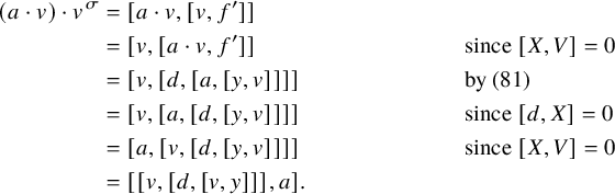 $$ \begin{align*} (a \cdot v) \cdot v^\sigma &= [a \cdot v, [v, f']] \\ &= [v, [a \cdot v, f']] && \text{since }[X, V] = 0 \\ &= [v, [d, [a, [y, v]]]] && \text{by (81)} \\ &= [v, [a, [d, [y, v]]]] && \text{since }[d, X] = 0 \\ &= [a, [v, [d, [y, v]]]] && \text{since }[X, V] = 0 \\ &= [[v, [d, [v, y]]], a]. \end{align*} $$
Now $[[v,d], [v,y]] = [v, [d, [v,y]]] - [d, [v, [v,y]]] = [v, [d, [v,y]]] + \lambda [c,d]$
for some
$[[v,d], [v,y]] = [v, [d, [v,y]]] - [d, [v, [v,y]]] = [v, [d, [v,y]]] + \lambda [c,d]$
for some $\lambda \in k$
because
$\lambda \in k$
because $[v, [v, y]] \in \langle c \rangle $
by the grading. By Proposition 2.4(ii), however,
$[v, [v, y]] \in \langle c \rangle $
by the grading. By Proposition 2.4(ii), however, $[[c,d], a] = 0$
, and hence,
$[[c,d], a] = 0$
, and hence,
 $$\begin{align*}(a \cdot v) \cdot v^\sigma = \big[ [[v,d], [v,y]], a \big]. \end{align*}$$
The result now follows from (70) together with Proposition 2.4(ii).
Lemma 5.34. Let $a,b \in X$
. Then
$a,b \in X$
. Then $[a,b] = - T(h(a,b), e)x$
. In particular, the bilinear map
$[a,b] = - T(h(a,b), e)x$
. In particular, the bilinear map
 $$\begin{align*}X \times X \to k \colon (a,b) \mapsto T(h(a,b), e) \end{align*}$$
is nondegenerate.
Proof. Using the definitions of T and h, we get
 $$\begin{align*}T(h(a,b), e)x = [h(a,b), [e,d]] = [[a, [b,f]], -e'] = [e', [a, [b, f]]]. \end{align*}$$
Since $[e', a] = [e', b] = 0$
, it follows that
$[e', a] = [e', b] = 0$
, it follows that
 $$\begin{align*}T(h(a,b), e)x = [a, [b, [e', f]]]. \end{align*}$$
Once again using (72) and Proposition 2.4(ii), we get $[b, [e', f]] = -b$
, and the required identity follows.
$[b, [e', f]] = -b$
, and the required identity follows.
Next, suppose that $a \in X$
is such that
$a \in X$
is such that $T(h(a,b), e) = 0$
for all
$T(h(a,b), e) = 0$
for all $b \in X$
. Then
$b \in X$
. Then $[a,b] = 0$
for all
$[a,b] = 0$
for all $b \in X$
. Since also
$b \in X$
. Since also $[a,V] = 0$
and
$[a,V] = 0$
and $[a, V'] = 0$
by the grading, this implies that
$[a, V'] = 0$
by the grading, this implies that $[a, L_{-1}] = 0$
. By Lemma 2.11, however, this implies
$[a, L_{-1}] = 0$
. By Lemma 2.11, however, this implies $a = 0$
, as required.
$a = 0$
, as required.
Corollary 5.35. Let $a,b \in X$
. Then
$a,b \in X$
. Then $h(a,b)^\sigma = -h(b,a)$
.
$h(a,b)^\sigma = -h(b,a)$
.
Proof. Since $[x,f] = -e$
, it follows from Lemma 5.34 that
$[x,f] = -e$
, it follows from Lemma 5.34 that
 $$\begin{align*}T(h(a,b), e) e = [[a,b], f] = [a, [b, f]] - [b, [a, f]] = h(a,b) - h(b,a). \end{align*}$$
Since $h(a,b)^\sigma = T(h(a,b), e)e - h(a,b)$
, the result follows.
$h(a,b)^\sigma = T(h(a,b), e)e - h(a,b)$
, the result follows.
Proposition 5.36. Let $a,b \in X$
and
$a,b \in X$
and $v\in V$
. Then
$v\in V$
. Then
 $$\begin{align*}T(h(a, b), v) = T(h(a \cdot v, b), e) = T(h(a, b \cdot v^\sigma), e). \end{align*}$$
Proof. Using the definition of T, Lemma 5.27(iv) and the fact that $[V, X] = 0$
, we get
$[V, X] = 0$
, we get
 $$\begin{align*}T(h(a, b), v)x = [v, [h(a,b), d]] = - [v, [a, [b, f']]] = - [a, [b, [v, f']]]. \end{align*}$$
By Lemma 5.32, we have $[b, [v, f']] = b \cdot v^\sigma $
, so together with Lemma 5.34, we get
$[b, [v, f']] = b \cdot v^\sigma $
, so together with Lemma 5.34, we get
 $$\begin{align*}T(h(a, b), v)x = - [a, b \cdot v^\sigma] = - T(h(a, b \cdot v^\sigma), e) x. \end{align*}$$
Next, since $\sigma $
is an involutory isometry of Q, we also have, using Corollary 5.35,
$\sigma $
is an involutory isometry of Q, we also have, using Corollary 5.35,
 $$ \begin{align*} T(h(a, b), v)x &= T(h(a,b)^\sigma, v^\sigma) x = - T(h(b,a), v^\sigma) x = - T(h(b, a \cdot v), e) x \\ &= - T(h(b, a \cdot v)^\sigma, e^\sigma) x = T(h(a \cdot v, b), e) x. \end{align*} $$
Proposition 5.37. Let $a,b \in X$
and
$a,b \in X$
and $v\in V$
. Then
$v\in V$
. Then
 $$\begin{align*}h(a, b\cdot v) = h(b, a \cdot v) + T(h(a, b), e)v. \end{align*}$$
Proof. By Proposition 5.31, we have
 $$\begin{align*}h(a, b \cdot v) - \gamma(a,b) v = h(b, a \cdot v) - \gamma(b,a) v. \end{align*}$$
Moreover, we have
 $$\begin{align*}\gamma(a,b) - \gamma(b,a) = T(h(a,b) - h(b,a), \delta), \end{align*}$$
so by Corollary 5.35, we get, using $T(e, \delta ) = 1$
, that
$T(e, \delta ) = 1$
, that
 $$\begin{align*}\gamma(a,b) - \gamma(b,a) = T \big( T(h(a,b), e)e, \delta \big) = T(h(a,b), e). \end{align*}$$
The result follows.
We now introduce some auxiliary notation.
Notation 5.38. Let $a \in X$
and let
$a \in X$
and let $\Theta _a$
be as in Definition 5.29. Then we can decompose
$\Theta _a$
be as in Definition 5.29. Then we can decompose
 $$\begin{align*}\Theta_a(y) = y + [a, y] + \ell_a + \tilde a + \lambda_a x \end{align*}$$
with $\ell _a \in L_0 \cap L^{\prime }_0$
,
$\ell _a \in L_0 \cap L^{\prime }_0$
, $\tilde a \in X$
and
$\tilde a \in X$
and $\lambda _a \in k$
.
$\lambda _a \in k$
.
It turns out that understanding the adjoint action of $\ell _a$
explicitly on the various components in the
$\ell _a$
explicitly on the various components in the $5 \times 5$
-grading gives a lot of insight, so this is what we will examine in the next few results.
$5 \times 5$
-grading gives a lot of insight, so this is what we will examine in the next few results.
Lemma 5.39. Let $a \in X$
. Then
$a \in X$
. Then $[\ell _a, c] = 0$
and
$[\ell _a, c] = 0$
and $[\ell _a, d] = 0$
.
$[\ell _a, d] = 0$
.
Proof. Since $\Theta _a(c) = c$
and
$\Theta _a(c) = c$
and $[y,c] = 0$
, we have
$[y,c] = 0$
, we have $[\Theta _a(y), c] = 0$
, so in particular,
$[\Theta _a(y), c] = 0$
, so in particular, $[\ell _a, c] = 0$
. The proof of
$[\ell _a, c] = 0$
. The proof of $[\ell _a, d] = 0$
is similar.
$[\ell _a, d] = 0$
is similar.
Lemma 5.40. Let $a \in X$
and
$a \in X$
and $v \in V$
. Then
$v \in V$
. Then
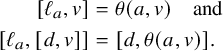 $$ \begin{align*} [\ell_a, v] &= \theta(a,v) \quad \text{and} \\ [\ell_a, [d,v]] &= [d, \theta(a,v)]. \end{align*} $$
Proof. Since $\Theta _a(v) = v$
, we have
$\Theta _a(v) = v$
, we have
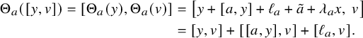 $$ \begin{align*} \Theta_a([y,v]) = [\Theta_a(y), \Theta_a(v)] &= \big[ y + [a, y] + \ell_a + \tilde a + \lambda_a x, \ v \big] \\ &= [y, v] + [[a,y], v] + [\ell_a, v]. \end{align*} $$
However, recall from (76) that
 $$\begin{align*}\Theta_a([y,v]) = [y,v] + [a \cdot v, f] + \theta(a,v). \end{align*}$$
Hence, $[\ell _a, v] = \theta (a,v)$
. Next, consider the automorphism
$[\ell _a, v] = \theta (a,v)$
. Next, consider the automorphism $\varphi $
from Lemma 2.8 with respect to the
$\varphi $
from Lemma 2.8 with respect to the $L^{\prime }_i$
-grading (55). Then by Lemmas 2.8 and 5.39,
$L^{\prime }_i$
-grading (55). Then by Lemmas 2.8 and 5.39,
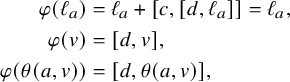 $$ \begin{align*} \varphi(\ell_a) &= \ell_a + [c, [d, \ell_a]] = \ell_a, \\ \varphi(v) &= [d, v], \\ \varphi(\theta(a,v)) &= [d, \theta(a,v)], \end{align*} $$
so the second identity follows from the first by applying $\varphi $
.
$\varphi $
.
Proposition 5.41. Let $a \in X$
and
$a \in X$
and $v \in V$
. Then
$v \in V$
. Then
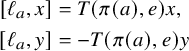 $$\begin{align*} [\ell_a, x] &= T(\pi(a), e) x, \notag \\ [\ell_a, y] &= - T(\pi(a), e) y \end{align*}$$
and
 $$ \begin{align} T(\theta(a,v), v) &= Q(v) T(\pi(a), e). \end{align} $$
Proof. Since $\Theta _a(x) = x$
, we have
$\Theta _a(x) = x$
, we have
 $$ \begin{align} \Theta_a([x,y]) = \big[ x, \ y + [a, y] + \ell_a + \tilde a + \lambda_a x \big] = [x,y] + a - [\ell_a, x]. \end{align} $$
We also have $\Theta _a([c,d]) = [\Theta _a(c), \Theta _a(d)] = [c,d]$
and
$\Theta _a([c,d]) = [\Theta _a(c), \Theta _a(d)] = [c,d]$
and $\Theta _a([d,v]) = [d,v]$
. We now apply
$\Theta _a([d,v]) = [d,v]$
. We now apply $\Theta _a$
to (70), so we get, using (76) and (83),
$\Theta _a$
to (70), so we get, using (76) and (83),
 $$\begin{align*}Q(v) \big( [c,d] - [x,y] - a + [\ell_a, x] \big) = \big[ [d,v], [y,v] + [a \cdot v, f] + \theta(a,v) \big]. \end{align*}$$
In particular, the $L_{-2}$
-components of both sides are equal, so we get
$L_{-2}$
-components of both sides are equal, so we get
 $$\begin{align*}Q(v) [\ell_a, x] = \big[ [d,v], \theta(a,v) \big] = T(\theta(a,v), v). \end{align*}$$
If we set $v = e$
, then we get
$v = e$
, then we get $[\ell _a, x] = T(\pi (a), e)$
. Substituting this again in the identity for general v then yields the third identity. Finally, to get the second identity, write
$[\ell _a, x] = T(\pi (a), e)$
. Substituting this again in the identity for general v then yields the third identity. Finally, to get the second identity, write $[\ell _a, y] = \mu y$
. Since
$[\ell _a, y] = \mu y$
. Since $[\ell _a, [x,y]] = 0$
by Proposition 2.4(ii), we have
$[\ell _a, [x,y]] = 0$
by Proposition 2.4(ii), we have $[[\ell _a, x], y] = [[\ell _a, y], x]$
and hence
$[[\ell _a, x], y] = [[\ell _a, y], x]$
and hence $\mu = - T(\pi (a), e)$
.
$\mu = - T(\pi (a), e)$
.
Corollary 5.42. Let $a \in X$
and
$a \in X$
and $v,w \in V$
. Then
$v,w \in V$
. Then
 $$\begin{align*}T(\theta(a,v), w) + T(\theta(a,w), v) = T(v,w) T(\pi(a), e) \end{align*}$$
and
 $$\begin{align*}\theta(a, v^\sigma)^\sigma = \theta(a,v) - T(e,v) \pi(a) + T(\pi(a), v)e. \end{align*}$$
Proof. The first identity follows by linearizing (82). If we choose $w = e$
, then we get
$w = e$
, then we get
 $$\begin{align*}T(\theta(a,v), e) + T(\pi(a), v) = T(v,e) T(\pi(a), e). \end{align*}$$
The second identity then follows from the definition of $\sigma $
together with this identity.
$\sigma $
together with this identity.
Lemma 5.43. Let $a,b \in X$
. Then
$a,b \in X$
. Then
 $$ \begin{align} [\ell_a, [b, f]] = - [ a \cdot h(a,b), f ] \end{align} $$
and
 $$ \begin{align} \theta(a, h(a,b)) + h(\tilde a, b) = 0. \end{align} $$
Proof. We have $[y, [b,f]] = 0$
by the grading, and hence,
$[y, [b,f]] = 0$
by the grading, and hence, $[\Theta _a(y), \Theta _a([b,f])] = 0$
. Recall from (79) that
$[\Theta _a(y), \Theta _a([b,f])] = 0$
. Recall from (79) that
 $$\begin{align*}\Theta_a([b,f]) = [b,f] + h(a,b) \in X' \oplus V. \end{align*}$$
Combining this with Notation 5.38, we get
 $$\begin{align*}\big[ y + [a, y] + \ell_a + \tilde a + \lambda_a x, \ [b,f] + h(a,b) \big] = 0. \end{align*}$$
In particular, the $L_0$
-component and
$L_0$
-component and $L_{-1}$
-component of the left-hand side are
$L_{-1}$
-component of the left-hand side are $0$
, so
$0$
, so
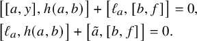 $$ \begin{align*} &\big[ [a,y], h(a,b) \big] + \big[ \ell_a, [b,f] \big] = 0, \\ &\big[ \ell_a, h(a,b) \big] + \big[ \tilde a, [b,f] \big] = 0. \end{align*} $$
Applying Lemma 5.27(ii) on the first identity now yields (84), and applying Lemma 5.40 and (73) on the second identity yields (85).
Lemma 5.44. Let $a \in X$
and
$a \in X$
and $v \in V$
. Then
$v \in V$
. Then
 $$ \begin{align} h(a, a \cdot v) + T(\pi(a), e)v = 2 \theta(a,v). \end{align} $$
In particular, $\pi (a)^\sigma = \pi (a) - h(a,a)$
. Moreover, we have
$\pi (a)^\sigma = \pi (a) - h(a,a)$
. Moreover, we have $T(\pi (a), e) = \gamma (a,a)$
and
$T(\pi (a), e) = \gamma (a,a)$
and $2 \gamma (a,a) = 0$
(i.e.,
$2 \gamma (a,a) = 0$
(i.e., $\gamma (a,a) = 0$
when
$\gamma (a,a) = 0$
when $\operatorname {\mathrm {char}}(k) \neq 2$
).
$\operatorname {\mathrm {char}}(k) \neq 2$
).
Proof. By Proposition 2.4(ii), we have $[[x,y], y] = 2y$
. Applying
$[[x,y], y] = 2y$
. Applying $\Theta _a$
and using Notation 5.38, Proposition 5.41, and (83) then gives
$\Theta _a$
and using Notation 5.38, Proposition 5.41, and (83) then gives
 $$\begin{align*}\big[ [x,y] + a - T(\pi(a), e)x, \ y + [a, y] + \ell_a + \tilde a + \lambda_a x \big] = 2 \big( y + [a, y] + \ell_a + \tilde a + \lambda_a x \big). \end{align*}$$
In particular, the $L_0$
-components of both sides are equal, so using
$L_0$
-components of both sides are equal, so using $[[x,y], \ell _a] = 0$
(by Proposition 2.4(ii) again), we get
$[[x,y], \ell _a] = 0$
(by Proposition 2.4(ii) again), we get
 $$\begin{align*}[a, [a, y]] - T(\pi(a), e) [x,y] = 2 \ell_a. \end{align*}$$
Now notice that by Lemma 5.27(iii) and using $[a,v] = 0$
, we have
$[a,v] = 0$
, we have $\big [ [a, [a,y]], v \big ] = h(a, a \cdot v)$
. Moreover,
$\big [ [a, [a,y]], v \big ] = h(a, a \cdot v)$
. Moreover, $[[x,y], v] = -v$
by Proposition 2.4(ii) again, and
$[[x,y], v] = -v$
by Proposition 2.4(ii) again, and $[\ell _a, v] = \theta (a,v)$
by Lemma 5.40, so we get (86). In particular, we have
$[\ell _a, v] = \theta (a,v)$
by Lemma 5.40, so we get (86). In particular, we have $h(a,a) + T(\pi (a), e)e = 2 \pi (a)$
, so
$h(a,a) + T(\pi (a), e)e = 2 \pi (a)$
, so
 $$\begin{align*}\pi(a)^\sigma = T(\pi(a), e)e - \pi(a) = \pi(a) - h(a,a). \end{align*}$$
Moreover, by Proposition 5.31 with $a=b$
and
$a=b$
and $v=e$
, we have
$v=e$
, we have
 $$\begin{align*}2 \pi(a) = h(a,a) - \gamma(a,a)e , \end{align*}$$
so by comparing with the previous identity, we get $T(\pi (a), e) = - \gamma (a,a)$
.
$T(\pi (a), e) = - \gamma (a,a)$
.
Finally, observe that when $\operatorname {\mathrm {char}}(k) \neq 2$
, then
$\operatorname {\mathrm {char}}(k) \neq 2$
, then $\delta = \tfrac {1}{2}e$
, so by Proposition 5.31,
$\delta = \tfrac {1}{2}e$
, so by Proposition 5.31, $\gamma (a,a) = T(h(a,a), \tfrac {1}{2} e)$
, which is
$\gamma (a,a) = T(h(a,a), \tfrac {1}{2} e)$
, which is $0$
by Lemma 5.34.
$0$
by Lemma 5.34.
Proposition 5.45. Let $a \in X$
and
$a \in X$
and $v \in V$
. Then
$v \in V$
. Then $\tilde a = - a \cdot \pi (a)^\sigma $
and
$\tilde a = - a \cdot \pi (a)^\sigma $
and
 $$ \begin{align} a \cdot \theta(a,v) = a \cdot \pi(a) \cdot v. \end{align} $$
Moreover, we have
 $$ \begin{align} \lambda_a v = \theta(a, \theta(a,v)) - h(a \cdot \pi(a)^\sigma, a \cdot v). \end{align} $$
Proof. We have $[y, [y,v]] = 0$
by the grading, and hence,
$[y, [y,v]] = 0$
by the grading, and hence, $[\Theta _a(y), \Theta _a([y,v])] = 0$
. By (76) and Notation 5.38, we get
$[\Theta _a(y), \Theta _a([y,v])] = 0$
. By (76) and Notation 5.38, we get
 $$ \begin{align} \big[ y + [a, y] + \ell_a + \tilde a + \lambda_a x, \ [y,v] + [a \cdot v, f] + \theta(a,v) \big] = 0. \end{align} $$
In particular, the $L_0$
-component of the left-hand side is
$L_0$
-component of the left-hand side is $0$
, so
$0$
, so
 $$\begin{align*}\big[ [a,y], \theta(a,v) \big] + \big[ \ell_a, [a \cdot v, f] \big] + \big[ \tilde a, [y, v] \big] = 0. \end{align*}$$
Now using Lemma 5.27(ii) for the first and third term and using (84) for the second term, we get
 $$\begin{align*}\big[ a \cdot \theta(a,v) - a \cdot h(a, a \cdot v) + \tilde a \cdot v, \ f \big] = 0, \end{align*}$$
and hence, by Corollary 5.24,
 $$\begin{align*}a \cdot \theta(a,v) - a \cdot h(a, a \cdot v) + \tilde a \cdot v = 0. \end{align*}$$
By (86), this can be rewritten as
 $$\begin{align*}\tilde a \cdot v = a \cdot \theta(a,v) - T(\pi(a), e) a \cdot v. \end{align*}$$
If we set $v = e$
, then we get
$v = e$
, then we get $\tilde a = - a \cdot \pi (a)^\sigma $
. Substituting this again in the previous identity, we get, using
$\tilde a = - a \cdot \pi (a)^\sigma $
. Substituting this again in the previous identity, we get, using $\pi (a)^\sigma = T(\pi (a), e)e - \pi (a)$
, that
$\pi (a)^\sigma = T(\pi (a), e)e - \pi (a)$
, that
 $$\begin{align*}a \cdot \theta(a,v) = - a \cdot \pi(a)^\sigma \cdot v + T(\pi(a), e) a \cdot v = a \cdot \pi(a) \cdot v. \end{align*}$$
To prove the second identity, we again start from (89), but this time we compute the $L_{-1}$
-component, so we get
$L_{-1}$
-component, so we get
 $$\begin{align*}\big[ \ell_a, \theta(a,v) \big] + \big[ \tilde a, [a \cdot v, f] \big] + \big[ \lambda_a x, [y,v] \big] = 0. \end{align*}$$
Using $\tilde a = - a \cdot \pi (a)^\sigma $
, (73) and Lemma 5.40, we get (88).
$\tilde a = - a \cdot \pi (a)^\sigma $
, (73) and Lemma 5.40, we get (88).
Lemma 5.46. Let $a \in X$
and
$a \in X$
and $v \in V$
. Then
$v \in V$
. Then
 $$\begin{align*}[\ell_a, [y, v]] = [y, \theta(a,v) - T(\pi(a), e)v]. \end{align*}$$
In particular, $[\ell _a, f] = - [y, \pi (a)^\sigma ]$
.
$[\ell _a, f] = - [y, \pi (a)^\sigma ]$
.
Proof. Using Lemma 5.40 and Proposition 5.41, we get
 $$\begin{align*}[\ell_a, [y, v]] = [[\ell_a, y], v] + [y, [\ell_a, v]] = - T(\pi(a), e)[y,v] + [y, \theta(a,v)]. \end{align*}$$
The second identity follows by setting $v = e$
since
$v = e$
since $f = [y, e]$
.
$f = [y, e]$
.
Lemma 5.47. Let $a,b \in X$
. Then
$a,b \in X$
. Then
 $$\begin{align*}[\ell_a, b] = b \cdot \pi(a)^\sigma - a \cdot h(a,b). \end{align*}$$
Proof. Using (84), Lemma 5.46 and Lemma 5.27(iii), we get
 $$ \begin{align*} [[\ell_a, b], f] = [\ell_a, [b, f]] - [b, [\ell_a, f]] &= - [a \cdot h(a,b), f] + [b, [y, \pi(a)^\sigma]] \\ &= [- a \cdot h(a,b) + b \cdot \pi(a)^\sigma, f]. \end{align*} $$
The result now follows from Corollary 5.24.
We can now explicitly determine the value of $\lambda _a$
introduced in Notation 5.38.
$\lambda _a$
introduced in Notation 5.38.
Proposition 5.48. Let $a \in X$
. Then
$a \in X$
. Then $\lambda _a = Q(\pi (a))$
.
$\lambda _a = Q(\pi (a))$
.
Proof. Since $\tilde a = - a \cdot \pi (a)^\sigma $
by Proposition 5.45, it follows from (85) with
$\tilde a = - a \cdot \pi (a)^\sigma $
by Proposition 5.45, it follows from (85) with $b=a$
that
$b=a$
that $h(a \cdot \pi (a)^\sigma , a) = \theta (a, h(a,a))$
, so by (87), we get
$h(a \cdot \pi (a)^\sigma , a) = \theta (a, h(a,a))$
, so by (87), we get
 $$ \begin{align} a \cdot h(a \cdot \pi(a)^\sigma, a) = a \cdot \pi(a) \cdot h(a,a). \end{align} $$
By (88) with $v = e$
, we have
$v = e$
, we have $\lambda _a e = \theta (a, \pi (a)) - h(a \cdot \pi (a)^\sigma , a)$
, and hence,
$\lambda _a e = \theta (a, \pi (a)) - h(a \cdot \pi (a)^\sigma , a)$
, and hence,
 $$\begin{align*}\lambda_a a = a \cdot \theta(a, \pi(a)) - a \cdot h(a \cdot \pi(a)^\sigma, a). \end{align*}$$
By (87) again and by (90), we can rewrite this as
 $$\begin{align*}\lambda_a a = a \cdot \pi(a) \cdot \pi(a) - a \cdot \pi(a) \cdot h(a,a). \end{align*}$$
Since $\pi (a) - h(a,a) = \pi (a)^\sigma $
by Lemma 5.44, we get, using Proposition 5.33, that
$\pi (a) - h(a,a) = \pi (a)^\sigma $
by Lemma 5.44, we get, using Proposition 5.33, that
 $$\begin{align*}\lambda_a a = a \cdot \pi(a) \cdot \pi(a)^\sigma = Q(\pi(a)) a.\\[-37pt] \end{align*}$$
We can now summarize our information about $\Theta _a(y)$
.
$\Theta _a(y)$
.
Corollary 5.49. Let $a \in X$
. Then
$a \in X$
. Then
 $$\begin{align*}\Theta_a(y) = y + [a, y] + \ell_a - a \cdot \pi(a)^\sigma + Q(\pi(a)) x. \end{align*}$$
We deduce another interesting identity, which is not required for the proof of our main result (Theorem 5.56), but which is interesting in its own right, and relevant also in the reconstruction process (see Remark 5.59 below).
Proposition 5.50. Let $a,b,c \in X$
. Write
$a,b,c \in X$
. Write $V_{a,b} := [a, [y,b]] \in L_0 \cap L^{\prime }_0$
. Then
$V_{a,b} := [a, [y,b]] \in L_0 \cap L^{\prime }_0$
. Then
 $$\begin{align*}[V_{a,b}, c] = a \cdot h(b,c) + b \cdot h(a,c) + c \cdot h(b,a). \end{align*}$$
Proof. We apply (78) on y and invoke Corollary 5.49 to get
 $$ \begin{align*} &\Theta_a \big( y + [b,y] + \ell_b - b \cdot \pi(b)^\sigma + Q(\pi(b)) x \big) \\ &\quad = \exp( -\gamma(a,b)x ) \big( y + [a+b,y] + \ell_{a+b} - (a+b) \cdot \pi(a+b)^\sigma + Q(\pi(a+b)) x \big). \end{align*} $$
Comparing the $L_0$
-component of both sides yields
$L_0$
-component of both sides yields
 $$\begin{align*}\ell_a + [a, [b,y]] + \ell_b = \ell_{a+b} - \gamma(a,b) [x,y]. \end{align*}$$
Taking the Lie bracket with $c \in X \leq L_{-1}$
now gives
$c \in X \leq L_{-1}$
now gives
 $$\begin{align*}[\ell_a, c] - [V_{a,b}, c] + [\ell_b, c] = [\ell_{a+b}, c] + \gamma(a,b) c. \end{align*}$$
We now apply Lemma 5.47, and we get
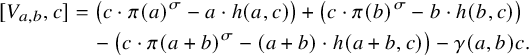 $$ \begin{align} [V_{a,b}, c] &= \big( c \cdot \pi(a)^\sigma - a \cdot h(a,c) \big) + \big( c \cdot \pi(b)^\sigma - b \cdot h(b,c) \big) \nonumber\\ &\quad- \big( c \cdot \pi(a+b)^\sigma - (a+b) \cdot h(a+b,c) \big) - \gamma(a,b) c. \end{align} $$
By (80) and Corollary 5.35, we have
 $$\begin{align*}c \cdot \pi(a+b)^\sigma = c \cdot \pi(a)^\sigma + c \cdot \pi(b)^\sigma - c \cdot h(b,a) - \gamma(a,b) c. \end{align*}$$
Substituting this expression in (91), the result follows.
Remark 5.51. The notation $V_{a,b}$
that we use is not a coincidence: the expression for
$V_{a,b}$
that we use is not a coincidence: the expression for $[V_{a,b}, c]$
is exactly the expression for the V-operators in the theory of structurable algebras (in characteristic
$[V_{a,b}, c]$
is exactly the expression for the V-operators in the theory of structurable algebras (in characteristic $\neq 2,3$
) related to quadrangular algebras. See [Reference Boelaert and De MedtsBDM13, Theorem 5.4].
$\neq 2,3$
) related to quadrangular algebras. See [Reference Boelaert and De MedtsBDM13, Theorem 5.4].
We have now arrived at the most difficult identity, which we will prove in Proposition 5.55 below. The crucial ingredient will be Lemma 5.53, proving the equality of certain products of automorphisms, which is, in fact, a typical ‘long commutator relation’ in disguise.
Similarly to Proposition 5.28 and Definition 5.29, we will need exponential maps for elements of $X'$
, with respect to the
$X'$
, with respect to the $L^{\prime }_i$
-grading (55).
$L^{\prime }_i$
-grading (55).
Definition 5.52.
-
(i) For each
$[a,f] \in X' \leq L^{\prime }_{-1}$
, we write
$\hat \Theta _a$
for the unique
$[a,f]$
-exponential automorphism
$\alpha \in \operatorname {\mathrm {Aut}}(L)$
such that
$[q_\alpha (e'), [d, \delta ]] = 0$
. The corresponding (uniquely defined) maps
$q_\alpha $
,
$n_\alpha $
and
$v_\alpha $
will be denoted by
$\hat q_a$
,
$\hat n_a$
and
$\hat v_a$
, respectively. -
(ii) For each
$a \in X$
and each
$v \in V$
, we define
$\hat \theta (a,v) := \hat q_a([d,v]) \in V$
. In particular, we have (92)where the second equality holds by Lemma 5.32 since
$$ \begin{align} \hat\Theta_a([d,v]) = [d,v] + [[a,f], [d,v]] + \hat\theta(a,v) = [d,v] + a \cdot v^\sigma + \hat\theta(a,v) , \end{align} $$
$f' = [d,f]$
.


For the next lemma, recall that $\alpha _{\theta (a,v)}$
and
$\alpha _{\theta (a,v)}$
and $\beta _v$
have been introduced in Definitions 5.15 and 5.16, respectively.
$\beta _v$
have been introduced in Definitions 5.15 and 5.16, respectively.
Lemma 5.53. Let $a \in X$
and
$a \in X$
and $v \in V$
. Then there is a (unique)
$v \in V$
. Then there is a (unique) $\mu =: \mu (a,v) \in k$
such that
$\mu =: \mu (a,v) \in k$
such that
 $$\begin{align*}\exp(- \mu c) \, \Theta_a \, \beta_v = \beta_v \, \hat\Theta_{a \cdot v} \, \alpha_{\theta(a,v)} \, \Theta_a. \end{align*}$$
Proof. Consider the automorphism $\beta := \Theta _a \, \beta _v \, \Theta _a^{-1}$
and recall that
$\beta := \Theta _a \, \beta _v \, \Theta _a^{-1}$
and recall that $\beta _v$
is a
$\beta _v$
is a $[y,v]$
-exponential automorphism with respect to the
$[y,v]$
-exponential automorphism with respect to the $L^{\prime }_i$
-grading (55). Write
$L^{\prime }_i$
-grading (55). Write
 $$\begin{align*}\beta_v = \operatorname{\mathrm{id}} + \operatorname{\mathrm{ad}}_{[y,v]} + q_{[y,v]} + n_{[y,v]} + v_{[y,v]}. \end{align*}$$
Now let $l_i \in L^{\prime }_i$
. Since
$l_i \in L^{\prime }_i$
. Since $\Theta _a$
preserves the
$\Theta _a$
preserves the $L^{\prime }_i$
-grading (55), also
$L^{\prime }_i$
-grading (55), also $\Theta _a^{-1}(l_i) \in L^{\prime }_i$
, so we can write
$\Theta _a^{-1}(l_i) \in L^{\prime }_i$
, so we can write
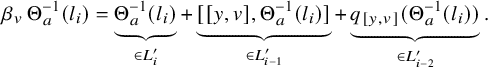 $$\begin{align*}\beta_v \, \Theta_a^{-1}(l_i) = \underbrace{\Theta_a^{-1}(l_i)}_{\in L^{\prime}_i} + \underbrace{[[y,v], \Theta_a^{-1}(l_i)]}_{\in L^{\prime}_{i-1}} + \underbrace{q_{[y,v]}(\Theta_a^{-1}(l_i))}_{\in L^{\prime}_{i-2}}. \end{align*}$$
Hence,
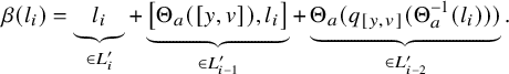 $$\begin{align*}\beta(l_i) = \underbrace{l_i}_{\in L^{\prime}_i} + \underbrace{\big[ \Theta_a([y,v]), l_i \big]}_{\in L^{\prime}_{i-1}} + \underbrace{\Theta_a(q_{[y,v]}(\Theta_a^{-1}(l_i)))}_{\in L^{\prime}_{i-2}}. \end{align*}$$
This shows that $\beta $
is an l-exponential automorphism for
$\beta $
is an l-exponential automorphism for $l = \Theta _a([y,v])$
, with respect to the
$l = \Theta _a([y,v])$
, with respect to the $L^{\prime }_i$
-grading (55). Now
$L^{\prime }_i$
-grading (55). Now
 $$\begin{align*}l = [y,v] + [a \cdot v, f] + \theta(a,v) , \end{align*}$$
so by Theorem 3.13(viii), also $\beta _v \, \hat \Theta _{a \cdot v} \, \alpha _{\theta (a,v)}$
is an l-exponential automorphism. (Notice that we have implicitly used Proposition 5.17 for
$\beta _v \, \hat \Theta _{a \cdot v} \, \alpha _{\theta (a,v)}$
is an l-exponential automorphism. (Notice that we have implicitly used Proposition 5.17 for $\alpha _{\theta (a,v)}$
here.) The result now follows from Theorem 3.13(v).
$\alpha _{\theta (a,v)}$
here.) The result now follows from Theorem 3.13(v).
Definition 5.54. Let $a \in X$
and
$a \in X$
and $v \in V$
. Then we set
$v \in V$
. Then we set
 $$\begin{align*}\phi(a,v) := \mu(a,v) - \mu(a \cdot v, e). \end{align*}$$
Proposition 5.55. Let $a \in X$
and
$a \in X$
and $v,w \in V$
. Then
$v,w \in V$
. Then
 $$\begin{align*}\hat\theta(a,v) = \theta(a, v^\sigma)^\sigma + \mu(a,e) v \end{align*}$$
and
 $$\begin{align*}\theta(a \cdot v, w^\sigma)^\sigma = Q(v) \theta(a,w) - T(v,w) \theta(a,v) + T(\theta(a,v), w)v + \phi(a,v)w. \end{align*}$$
Proof. We apply both sides of Lemma 5.53 to $[d,w] \in V'$
, and we extract the V-component of the resulting equality (so there are many terms that we do not need to compute explicitly). We first compute
$[d,w] \in V'$
, and we extract the V-component of the resulting equality (so there are many terms that we do not need to compute explicitly). We first compute
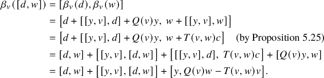 $$ \begin{align*} \beta_v([d,w]) &= [\beta_v(d), \beta_v(w)] \\ &= \big[ d + [[y,v], d] + Q(v)y , \ w + [[y,v], w] \big] \\ &= \big[ d + [[y,v], d] + Q(v)y , \ w + T(v,w)c \big] \quad \text{(by Proposition~}{5.25}) \\ &= [d,w] + \big[ [y,v], [d,w] \big] + \big[ [[y,v], d], \ T(v,w)c \big] + [Q(v)y, w] \\ &= [d,w] + \big[ [y,v], [d,w] \big] + \big[ y, Q(v)w - T(v,w)v \big]. \end{align*} $$
After applying $\exp (-\mu (a,v) c) \Theta _a$
on
$\exp (-\mu (a,v) c) \Theta _a$
on $\beta _v([d,w])$
, we see from the grading in Figure 2 that only two terms contribute to the V-component, namely
$\beta _v([d,w])$
, we see from the grading in Figure 2 that only two terms contribute to the V-component, namely
 $$\begin{align*}\exp(-\mu(a,v) c)([d,w]) \quad \text{and} \quad \Theta_a \big( \big[ y, Q(v)w - T(v,w)v \big] \big) , \end{align*}$$
and the resulting V-component is equal to
 $$ \begin{align} \mu(a,v) w + Q(v) \theta(a,w) - T(v,w) \theta(a,v). \end{align} $$
We now compute the V-component of
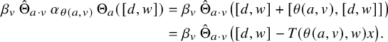 $$ \begin{align*} \beta_v \, \hat\Theta_{a \cdot v} \, \alpha_{\theta(a,v)} \, \Theta_a([d,w]) &= \beta_v \, \hat\Theta_{a \cdot v} \big( [d,w] + [\theta(a,v), [d,w]] \big) \\ &= \beta_v \, \hat\Theta_{a \cdot v} \big( [d,w] - T(\theta(a,v), w)x \big). \end{align*} $$
Again, only two terms contribute, namely
 $$\begin{align*}\hat\Theta_{a \cdot v}([d,w]) \quad \text{and} \quad \beta_v\big( - T(\theta(a,v), w)x \big) , \end{align*}$$
and the resulting V-component is equal to
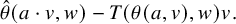 $$ \begin{align} \hat\theta(a \cdot v, w) - T(\theta(a,v), w) v. \end{align} $$
Since the expressions in (93) and (94) coincide, we get
 $$ \begin{align} \hat\theta(a \cdot v, w) = Q(v) \theta(a,w) - T(v,w) \theta(a,v) + T(\theta(a,v), w) v + \mu(a,v) w. \end{align} $$
Setting $v = e$
and invoking Corollary 5.42 then gives
$v = e$
and invoking Corollary 5.42 then gives
 $$ \begin{align*} \hat\theta(a, w) &= \theta(a,w) - T(e,w) \pi(a) + T(\pi(a), w) e + \mu(a,e) w \\ &= \theta(a, w^\sigma)^\sigma + \mu(a,e) w. \end{align*} $$
Finally, substituting $a \cdot v$
for a in this identity gives
$a \cdot v$
for a in this identity gives
 $$\begin{align*}\hat\theta(a \cdot v, w) = \theta(a \cdot v, w^\sigma)^\sigma + \mu(a \cdot v, e) w. \end{align*}$$
Comparing this with (95) gives the required identity.
We have now assembled all that is required to prove our main result of this section.
Theorem 5.56. Let L be as in Assumption 5.1, let V and X be as in Notation 5.4, let Q and T be as in Definition 5.10, let e and $\delta $
be as in Definition 5.21, let h and
$\delta $
be as in Definition 5.21, let h and $\cdot $
be as in Definition 5.26 and let
$\cdot $
be as in Definition 5.26 and let $\theta $
be as in Definition 5.29.
$\theta $
be as in Definition 5.29.
Then the system $(k,V,Q,T,e,X,\cdot ,h,\theta )$
is a quadrangular algebra, which is
$(k,V,Q,T,e,X,\cdot ,h,\theta )$
is a quadrangular algebra, which is $\delta $
-standard and for which both T and the bilinear map
$\delta $
-standard and for which both T and the bilinear map $X \times X \to k \colon (a,b) \mapsto T(h(a,b), e)$
are nondegenerate (so in particular, h is nodegenerate).
$X \times X \to k \colon (a,b) \mapsto T(h(a,b), e)$
are nondegenerate (so in particular, h is nodegenerate).
Proof. We first observe that $Q \colon V \to k$
is a regular quadratic form with associated bilinear form T, by Definition 5.10 and Lemma 5.18, so in fact, T is nondegenerate. By Definition 5.21,
$Q \colon V \to k$
is a regular quadratic form with associated bilinear form T, by Definition 5.10 and Lemma 5.18, so in fact, T is nondegenerate. By Definition 5.21, $e \in V$
is a base point for Q. By definition, the maps
$e \in V$
is a base point for Q. By definition, the maps $\cdot \colon X \times V \to X$
and
$\cdot \colon X \times V \to X$
and $h \colon X \times X \to V$
defined in Definition 5.26 are bilinear maps. Finally, the map
$h \colon X \times X \to V$
defined in Definition 5.26 are bilinear maps. Finally, the map $\theta \colon X \times V \to V$
has been introduced in Definition 5.29.
$\theta \colon X \times V \to V$
has been introduced in Definition 5.29.
We now verify each of the defining axioms (i)–(ix) from Definition 1.17.
-
(i) This is Lemma 5.27(i).
-
(ii) This is Proposition 5.33.
-
(iii) This is Proposition 5.37.
-
(iv) This is Proposition 5.36.
-
(v) This follows from the definition of
$\theta $
in Definition 5.29 because for each
$a \in X$
,
$\Theta _a$
is a linear map. -
(vi) This was observed already in Definition 5.29.
-
(vii) This is Proposition 5.31.
-
(viii) This is Proposition 5.55.
-
(ix) This is Proposition 5.45.


This shows that $(k,V,Q,T,e,X,\cdot ,h,\theta )$
is a quadrangular algebra. By Definition 5.21 and (77), it is
$(k,V,Q,T,e,X,\cdot ,h,\theta )$
is a quadrangular algebra. By Definition 5.21 and (77), it is $\delta $
-standard. Finally, the bilinear map
$\delta $
-standard. Finally, the bilinear map $X \times X \to k \colon (a,b) \mapsto T(h(a,b), e)$
is nondegenerate by Lemma 5.34.
$X \times X \to k \colon (a,b) \mapsto T(h(a,b), e)$
is nondegenerate by Lemma 5.34.
Remark 5.57. The conditions on the quadrangular algebra in the statement of Theorem 5.56 imply that if $X \neq 0$
, then either the quadrangular algebra is ‘generic’ (as in [Reference Mühlherr and WeissMW19, §8]) or it is ‘of split type
$X \neq 0$
, then either the quadrangular algebra is ‘generic’ (as in [Reference Mühlherr and WeissMW19, §8]) or it is ‘of split type $F_4$
’ (as in [Reference Mühlherr and WeissMW19, §10]). (We ignore the detail that
$F_4$
’ (as in [Reference Mühlherr and WeissMW19, §10]). (We ignore the detail that $|K|>4$
is required in the generic case in [Reference Mühlherr and WeissMW19, Hypothesis 8.1] and
$|K|>4$
is required in the generic case in [Reference Mühlherr and WeissMW19, Hypothesis 8.1] and $|K|>3$
is required in the split
$|K|>3$
is required in the split $F_4$
-case in [Reference Mühlherr and WeissMW19, Hypothesis 10.1].) Notice, however, that we allow the situation where
$F_4$
-case in [Reference Mühlherr and WeissMW19, Hypothesis 10.1].) Notice, however, that we allow the situation where $X = 0$
, in which case the quadrangular algebra is nothing more than a nondegenerate quadratic space with base point.
$X = 0$
, in which case the quadrangular algebra is nothing more than a nondegenerate quadratic space with base point.
Remark 5.58. When the quadrangular algebra is anisotropic, it ought to be possible to show that the resulting inner ideal geometry is a Moufang generalized quadrangle and that it is isomorphic to the Moufang quadrangle obtained from the quadrangular algebra as in [Reference WeissWei06]. (Notice that in this case, the extremal geometry has no lines. The inner ideal geometry is the geometry with point set ${\mathcal {E}}(L)$
and as line set the collection of inner ideals containing at least two extremal points and minimal with respect to this property.)
${\mathcal {E}}(L)$
and as line set the collection of inner ideals containing at least two extremal points and minimal with respect to this property.)
The explicit computations might be lengthy in general, but in the case that $\operatorname {\mathrm {char}}(k) \neq 2$
, this has been worked out in [Reference MeulewaeterMeu21, §4.5.2].
$\operatorname {\mathrm {char}}(k) \neq 2$
, this has been worked out in [Reference MeulewaeterMeu21, §4.5.2].
Remark 5.59. We are confident that, similarly to Corollary 4.17, the Lie algebra can be completely reconstructed from the quadrangular algebra, but we have not worked out the details. This time, we let
 $$\begin{align*}K_0 := \langle [x,y], [c,d] \rangle \oplus [X, [y,X]] \oplus [V, [y, V']] , \end{align*}$$
and we follow exactly the same procedure as in the proof of Corollary 4.17. However, working out all the different cases of Lie brackets between the $13$
different pieces in the grading requires substantially more computational effort than in the case of Section 4, and one crucial ingredient seems to be Proposition 5.50. We leave the details to the courageous reader.
$13$
different pieces in the grading requires substantially more computational effort than in the case of Section 4, and one crucial ingredient seems to be Proposition 5.50. We leave the details to the courageous reader.
Remark 5.60. As we can see, there is a third interesting grading on the Lie algebra L that we obtain from the diagonals in Figure 2. (There is, of course, also a fourth grading from the other diagonals.) Notice that this time, the ends of the grading are not one-dimensional! More precisely, we have
 $$\begin{align*}L = L^{\prime\prime}_{-2} \oplus L^{\prime\prime}_{-1} \oplus L^{\prime\prime}_0 \oplus L^{\prime\prime}_1 \oplus L^{\prime\prime}_2 \end{align*}$$
with
 $$ \begin{align*} L^{\prime\prime}_{-2} &= \langle x \rangle \oplus V \oplus \langle c \rangle \\ L^{\prime\prime}_{-1} &= X \oplus X' \\ L^{\prime\prime}_{0} &= V' \oplus (L_0 \cap L^{\prime}_0) \oplus [y,V] \\ L^{\prime\prime}_{1} &= [d, X'] \oplus [y,X] \\ L^{\prime\prime}_{2} &= \langle d \rangle \oplus [y,V'] \oplus \langle y \rangle. \end{align*} $$
This grading has been used implicitly in [Reference Boelaert and De MedtsBDM15] in the context of J-ternary algebras. See in particular its Theorem 3.5, where the Jordan algebra J is of the form $k \oplus V \oplus k$
, and where the space called X plays the role of
$k \oplus V \oplus k$
, and where the space called X plays the role of $L^{\prime \prime }_{\pm 1}$
and admits a Peirce decomposition into two isomorphic parts
$L^{\prime \prime }_{\pm 1}$
and admits a Peirce decomposition into two isomorphic parts $X = X_0 \oplus X_1$
(introduced in its Lemma 3.4).
$X = X_0 \oplus X_1$
(introduced in its Lemma 3.4).
A Tables
In this appendix, we present an overview of the possible Lie algebras of exceptional type that arise in this context. For each of the two situations (cubic norm structures vs. quadrangular algebras), we present two tables:
-
○ We first list the dimensions of the different pieces in the decomposition of the Lie algebra, depending only on the absolute type of the Lie algebra.
-
○ We then present a more detailed table with the possible Tits indices along with the corresponding precise form of the algebraic structure.
We do not provide proofs, and we rely instead on the corresponding information for Tits hexagons (taken from [Reference Mühlherr and WeissMW22]) and Tits quadrangles (taken from [Reference Mühlherr and WeissMW19]), respectively. Providing a direct connection between Tits hexagons and Tits quadrangles of index type and our Lie algebras is an interesting project in its own right. (See also Remarks 4.25 and 5.58.)
A.1 Cubic norm structures
In the case of cubic norm structures, corresponding to the $G_2$
-grading as in Figure 1 on p. 32, we see that
$G_2$
-grading as in Figure 1 on p. 32, we see that
 $$\begin{align*}\dim L = 6 + 6 \dim J + \dim (L_0 \cap L^{\prime}_0). \end{align*}$$
We have listed the six possibilities in Table 1.
In Table 2, we rely on [Reference Mühlherr and WeissMW22, Theorem 2.5.22], and we adopt its notation $\mathcal {H}(C, k)$
for the Freudenthal algebra constructed from the composition algebra C over k. (See also [Reference Mühlherr and WeissMW22, Notation 4.1.72].)
$\mathcal {H}(C, k)$
for the Freudenthal algebra constructed from the composition algebra C over k. (See also [Reference Mühlherr and WeissMW22, Notation 4.1.72].)
Remark A.1. The example of type $D_4$
in the second row of Table 2 also occurs in non-triality forms, which we have not included in the list because they are not exceptional. These correspond to the Tits indices
$D_4$
in the second row of Table 2 also occurs in non-triality forms, which we have not included in the list because they are not exceptional. These correspond to the Tits indices
and have corresponding $3$
-dimensional J of the form
$3$
-dimensional J of the form $J = k \times E$
, where
$J = k \times E$
, where $E/k$
is a separable quadratic field extension, for the first case, and of the form
$E/k$
is a separable quadratic field extension, for the first case, and of the form $J = k \times k \times k$
, a split cubic étale extension, for the second case.
$J = k \times k \times k$
, a split cubic étale extension, for the second case.
A.2 Quadrangular algebras
In the case of quadrangular algebras, corresponding to the $BC_2$
-grading as in Figure 2 on p. 42, we see that
$BC_2$
-grading as in Figure 2 on p. 42, we see that
 $$\begin{align*}\dim L = 4 + 4 \dim X + 4 \dim V + \dim (L_0 \cap L^{\prime}_0). \end{align*}$$
We have listed the four possibilities in Table 3.
By Remark 5.57, our quadrangular algebras are either generic or of split type $F_4$
. By [Reference Mühlherr and WeissMW19, Theorems 8.16 and 10.16], these are either special (i.e., not exceptional), or they are anisotropic, or they are isotopic to
$F_4$
. By [Reference Mühlherr and WeissMW19, Theorems 8.16 and 10.16], these are either special (i.e., not exceptional), or they are anisotropic, or they are isotopic to $\mathcal {Q}_2(C, k)$
for some octonion algebra C or to
$\mathcal {Q}_2(C, k)$
for some octonion algebra C or to $\mathcal {Q}_4(C, k)$
for some composition algebra C. (The definition of these quadrangular algebras can be found in [Reference Mühlherr and WeissMW19, Notations 4.12 and 4.14].) In other words, we get all cases from [Reference Mühlherr and WeissMW19, Table 1] except the last two rows. We have essentially reproduced this table in Table 4.
$\mathcal {Q}_4(C, k)$
for some composition algebra C. (The definition of these quadrangular algebras can be found in [Reference Mühlherr and WeissMW19, Notations 4.12 and 4.14].) In other words, we get all cases from [Reference Mühlherr and WeissMW19, Table 1] except the last two rows. We have essentially reproduced this table in Table 4.
Table 1 Dimensions of the pieces for the $G_2$
-grading.
$G_2$
-grading.
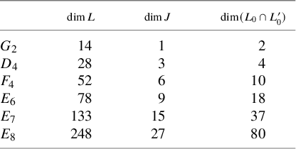
Table 2 Exceptional Tits indices with $G_2$
-graded Lie algebra
$G_2$
-graded Lie algebra
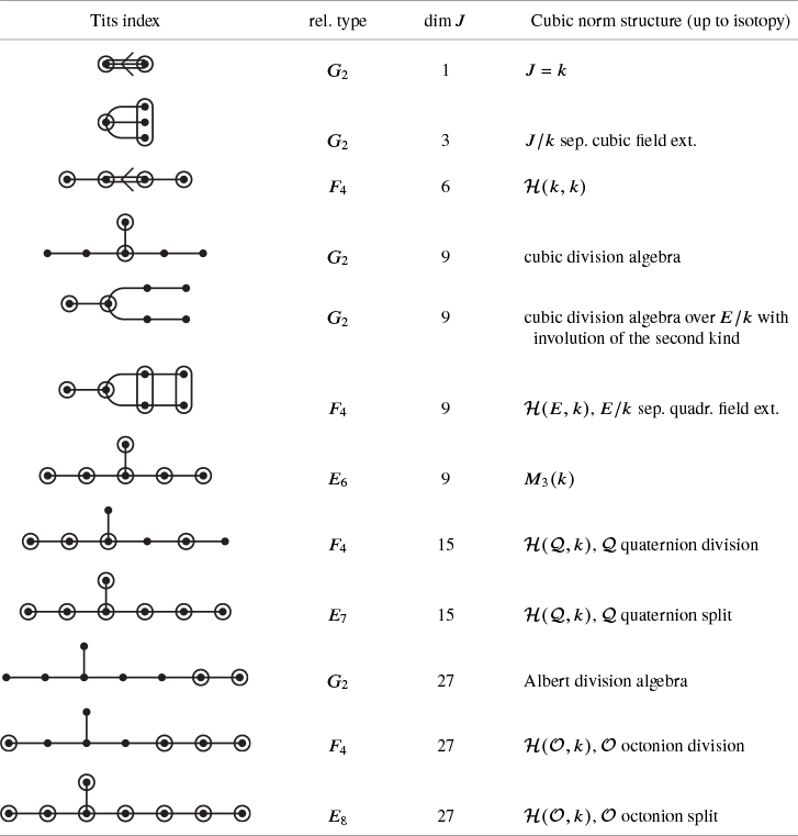
Remark A.2. Comparing Tables 2 and 4, we see that the Tits indices that occur in both tables are the following:
-
(i) The split forms of type
$F_4$
,
$E_6$
,
$E_7$
and
$E_8$
; -
(ii) The forms of relative type
$F_4$
(and of absolute type
$F_4$
,
$E_6$
,
$E_7$
and
$E_8$
).


In other words, these seven types of Lie algebras are precisely the ones admitting both a $G_2$
-grading and a
$G_2$
-grading and a $BC_2$
-grading, and hence, they are parametrized both by a cubic norm structure and by a quadrangular algebra. As we have alluded to in the introduction, it is an interesting question to investigate the connection between these two different algebraic structures for each of these seven types.
$BC_2$
-grading, and hence, they are parametrized both by a cubic norm structure and by a quadrangular algebra. As we have alluded to in the introduction, it is an interesting question to investigate the connection between these two different algebraic structures for each of these seven types.
Table 3 Dimensions of the pieces for the $BC_2$
-grading.
$BC_2$
-grading.

Table 4 Exceptional Tits indices with $BC_2$
-graded Lie algebra
$BC_2$
-graded Lie algebra
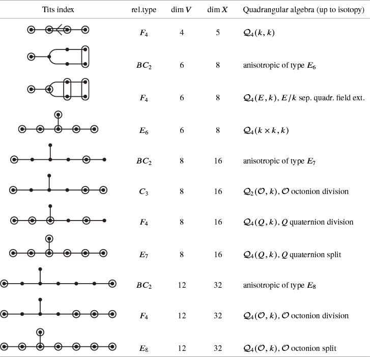
Acknowledgements
This work has been initiated as part of the PhD project of the second author [Reference MeulewaeterMeu21].
The first author has presentedFootnote 4 a preliminary version of these results at the Collège de France on the occasion of the ‘Colloque pour honorer la mémoire de Jacques Tits’ (11–13 December 2023). We thank the organizers and the Fondation Hugo du Collège de France for the invitation.
We are grateful to Michel Brion and Erhard Neher for their comments on that occasion, which have encouraged us to write down our results in the current form. We thank Vladimir Chernousov and Arjeh Cohen for the discussions about the origin of the terminology of extremal elements, and Holger Petersson for providing us with the reference [Reference FaulknerFau01] for cubic norm pairs.
We thank both referees for their valuable comments and their interesting suggestions for future research.
Competing interest
The authors have no competing interests to declare.
Funding statement
This research was supported by the Research Foundation Flanders (Belgium) (F.W.O.- Vlaanderen), grant 166032/1128720N.


 Open access