


1. Introduction
Stochastic differential equations (SDEs) evolving on linear spaces are well studied, and some of the popular books in this area are [Reference Arnold6, Reference Oksendal24]. The area of stochastic analysis on manifolds originated after K. Itô first described the coordinate transformation rules in [Reference Itô16]. Since then, the subject has evolved into what is now broadly called the stochastic differential geometry. However, many research areas in stochastic differential geometry do not particularly deal with SDEs on manifolds, which is the central theme of this article.
In linear spaces, Stratonovich SDE representation and Itô SDE representation are two popular ways of representing semimartingales in the form of SDEs. Therefore, it is natural that there will be equivalent ways of describing SDEs on manifolds. In the case of Stratonovich SDEs on manifolds, one finds that it is enough to consider sections of the tangent bundle (vector fields) to describe the drift and the noise coefficients. However, this is not true for Itô-type SDEs due to the additional drift correction term. To address this problem, L. Schwartz, in [Reference Schwartz25], introduced the idea of the second-order tangent bundle. One of the central ideas in Schwartz’s Stochastic Differential Geometry is the treatment of infinitesimal stochastic increment as an element of Schwartz’s second-order tangent space. These infinitesimal stochastic increments are also called Schwartz differentials. A complete account of Schwartz’s second-order geometry can be found in [Reference Émery2]. In the book [Reference Gliklikh14], Itô SDEs on manifolds are formulated using the idea of Itô bundle. As per this approach, if a manifold is equipped with a connection, it is possible to describe an Itô SDE on a manifold as a section of the Itô bundle. The book also describes Itô SDEs on manifolds using the Belopolskya–Daletskii form (Section 7.3 of [Reference Gliklikh14]), which can be exploited for numerical computations. Yet another approach to describe SDEs on manifolds is that of stochastic development and anti-development, which can be found in Chapter 2 of [Reference Hsu15] or in [Reference Elworthy12]. In this article, we are only interested in Schwartz’s approach to describe the SDEs.
In Schwartz’s approach, an SDE is described using the Schwartz morphism that morphs a semimartingale from a source manifold into a semimartingale on a target manifold. If we consider the source manifold as  $\mathbb{R}^{p}$ and the target manifold as
  $M$, with
  $X_t$ as a semimartingale on
  $\mathbb{R}^{p}$, then a Schwartz morphism can convert the semimartingale
  $X_t\in \mathbb{R}^{p}$ into a semimartingale on the target manifold
  $M$. Moreover, for a map
  $F:\mathbb{R}^{p}\to M$, there exists a Schwartz morphism that morphs the semimartingale
  $X_t\in \mathbb{R}^{p}$ into the semimartingale
  $F(X_t)\in M$.
In this article, we focus on the Schwartz morphisms that morph the process  $(t,W_t)\in \mathbb{R}^{p+1}$ into a semimartingale on
  $M$, which can also be described in terms of vector fields and a Schwartz’s second-order vector field (also called diffusor field in this article). In this article, we observe that it is possible to construct diffusor fields using special maps that we call diffusion generators. Hence, the idea of diffusion generator serves as an alternative viewpoint for the Schwartz morphism approach to describe SDEs on manifolds (when the driving process is
  $(t,W_t)\in \mathbb{R}^{p+1}$).
A recent approach in [Reference Armstrong and Brigo5] uses the idea of 2-jets to describe SDEs on manifolds, which can be interpreted as constructing the Schwartz morphism using 2-jet of a function  $F:\mathbb{R}^p \to M$. Our idea of the diffusion generator and its construction using the flow of differential equations can be seen as an extension of the 2-jet formulation for the SDEs on manifolds. Our work in this article is an exploration in the following three directions.
(i) Construction of Schwartz morphisms and diffusion generators. In Section 2, we demonstrate that it is possible to construct Schwartz morphisms using a diffusion generator and a set of vector fields. Like Schwartz’s approach, the diffusion generator approach also generalizes the Stratonovich representation and the Itô representation of SDEs. This is demonstrated by constructing diffusion generators using the flow of differential equations. We observe that in the case of a diffusion generator obtained by considering the flow of a first-order vector field, we end up with a Stratonovich SDE. Similarly, in the case of a manifold with a connection, considering the geodesic equation, the corresponding SDE is nothing but the Itô SDE.
(ii) Lagrangian mechanics and diffusion generators. Based on the diffusion generator approach, in Section 3, we show that in addition to Stratonovich representation and the Itô representation of SDEs, it is possible to have yet another representation of SDEs by defining a canonical diffusion generator using a regular Lagrangian. This is achieved by constructing a diffusion generator using the flow of the Euler–Lagrange equation with a regular Lagrangian. We call this canonical diffusion generator the Lagrangian diffusion generator. We demonstrate that it is possible to write the equations of motion in mechanics in terms of the Lagrangian diffusion generator.
(iii) Extended Itô formula on manifolds using diffusion generators. If
 $F:\mathbb{R}\times M\to N$, such that
$F(t,x)$ is a semimartingale for every
$x\in M$ and
$X_t$ is a semimartingale on
$M$, then the SDE representation for the semimartingale
$F(t,X_t)$ is not a straightforward application of the Schwartz morphism. In Euclidean spaces, the SDE for
$F(t,X_t)$ is given by the extended Itô formula [Reference Kunita19] (the extended Itô formula is also known as the generalized Itô formula or the Itô–Wentzell formula (also spelled Itô–Ventzel)). We give a representation conversion formula to convert the SDE representation of a stochastic process from one diffusion generator to another. Finally, using this conversion formula, we derive the extended Itô formula on the manifolds in the framework of diffusion generators.
$F:\mathbb{R}\times M\to N$, such that
$F(t,x)$ is a semimartingale for every
$x\in M$ and
$X_t$ is a semimartingale on
$M$, then the SDE representation for the semimartingale
$F(t,X_t)$ is not a straightforward application of the Schwartz morphism. In Euclidean spaces, the SDE for
$F(t,X_t)$ is given by the extended Itô formula [Reference Kunita19] (the extended Itô formula is also known as the generalized Itô formula or the Itô–Wentzell formula (also spelled Itô–Ventzel)). We give a representation conversion formula to convert the SDE representation of a stochastic process from one diffusion generator to another. Finally, using this conversion formula, we derive the extended Itô formula on the manifolds in the framework of diffusion generators.


Before giving a detailed overview of the article in Section 1.2, we will present some pre-existing notions and results from Schwartz’s stochastic differential geometry and basic Lagrangian mechanics in Section 1.1.
1.1. Review of basic notations and definitions, Schwartz’s stochastic differential geometry, and basic Lagrangian mechanics
We will denote the set of all sections of any fibre bundle  $F$ by
  $\Gamma(F)$. The set of all smooth vector fields will be denoted by
  $\mathfrak{X}(M)$ and the set of all smooth functions by
  $\mathfrak{F}(M)$. The natural pairing between a covector
  $\alpha_x\in T^*M$ and a vector
  $v_x\in TM$ will be simply denoted by the dot product in order
  $\alpha_x\cdot v_x$.
1.1.1. Schwartz’s stochastic differential geometry
Schwartz’s second-order tangent space at a point  $x$ on an n-manifold
  $M$ is defined as a vector space of all differential operators of up to order 2 at point
  $x$. We will denote it by
  $\mathfrak{D}_xM$. Locally, every second-order differential operator is symmetric and is represented as
  $\partial^2_{ij}$. Therefore, every differential operator up to the second-order is locally of the form
 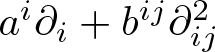 $a^i\partial_i + b^{ij}\partial^2_{ij}$. The symmetry of second-order differential operators means that the dimension of the second-order tangent space is
 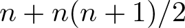 $n + n(n+1)/2$. We will call the elements of Schwartz’s second-order tangent space
  $\mathfrak{D}_xM$ as diffusors at point
  $x\in M$. With these definitions, it is clear that a tangent vector is also a diffusor, i.e.,
 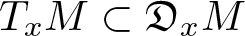 $T_xM\subset\mathfrak{D}_xM$
  $\forall$
  $x\in M$.
For any manifolds  $M$ and
  $N$, consider
  $L\in \mathfrak{D}_xM$; if
  $\phi:M\to N$, then the push forward of
  $L$ by
  $\phi$ at a specific point
  $x\in M$ is written as
  $\mathfrak{D}_x\phi (L)$, where
 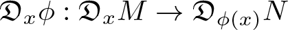 $\mathfrak{D}_x\phi:\mathfrak{D}_xM\to \mathfrak{D}_{\phi(x)}N$. Moreover,
  $\forall f\in \mathfrak{F}(N)$,
  $\mathfrak{D}_x\phi (L) [f] = L[f(\phi)] = L[\phi^*f]$. This push-forward map is linear. The fibre bundle over the manifold
  $M$, with Schwartz’s second-order tangent space
  $\mathfrak{D}_xM$ as the fibres, is called Schwartz’s second-order tangent bundle. For brevity, we will call Schwartz’s second-order tangent bundle as diffusion bundle, and Schwartz’s second-order tangent space as diffusion space. A smooth diffusor field
  $\zeta$ is defined as a smooth section of the diffusion bundle
  $\mathfrak{D}M$. Following our usual symbol for a section of a fibre bundle, we will denote the set of all smooth diffusor fields by
  $\Gamma(\mathfrak{D}M)$. For
  $\phi:M\to N$, we will call the fibre-preserving map over
  $\phi$,
 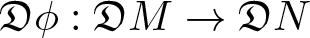 $\mathfrak{D}\phi:\mathfrak{D}M\to \mathfrak{D}N$ as the diffusion map. Locally in the charts
  $(U,\Upsilon)$ on
  $M$ and
  $(V,\chi)$ on
  $N$, for all
  $L\in \mathfrak{D}M$ such that
 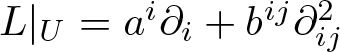 $L|_U = a^i\partial_i + b^{ij}\partial^2_{ij}$,
 \begin{equation}
\mathfrak{D}\phi \left(L\right)|_V = \left[ a^i\partial_i\phi^k + b^{ij}\partial^2_{ij}\phi^k\right] \partial_k + \left[b^{ij}\partial_i\phi^k \partial_j\phi^l\right]\partial^2_{kl}.
\end{equation}
\begin{equation}
\mathfrak{D}\phi \left(L\right)|_V = \left[ a^i\partial_i\phi^k + b^{ij}\partial^2_{ij}\phi^k\right] \partial_k + \left[b^{ij}\partial_i\phi^k \partial_j\phi^l\right]\partial^2_{kl}.
\end{equation} Given  $L\in \mathfrak{D}_xM$, consider a symmetric contravariant tensor
  $\hat{L}\in {T}^2_0M$ such that
 \begin{equation}
\hat{L}(df(x), dg(x)) = \dfrac{1}{2}(L[f(x)g(x)] - f(x)L[g(x)] - g(x)L[f(x)]).
\end{equation}
\begin{equation}
\hat{L}(df(x), dg(x)) = \dfrac{1}{2}(L[f(x)g(x)] - f(x)L[g(x)] - g(x)L[f(x)]).
\end{equation} The fact that  $\hat{L}$ is indeed symmetric can be verified locally by considering
  $L = a^i\partial_i + b^{ij}\partial^2_{ij}$. So, locally
 \begin{equation}
\hat{L}(df(x),dg(x)) = b^{ij}\partial_if\partial_jg.
\end{equation}
\begin{equation}
\hat{L}(df(x),dg(x)) = b^{ij}\partial_if\partial_jg.
\end{equation} A stochastic process  $X_t$ on a manifold
  $M$ is said to be a semimartingale if
  $f(X_t)$ is a semimartingale
  $\forall$
  $f\in \mathfrak{F}(M)$. Let
  $X_t$ be a continuous semimartingale on the manifold
  $M$. If
  $X_t^i$ are the local components of
  $X_t$ in some chart, then the local Itô differentials
  $dX_t^i$ and
  $\dfrac{1}{2}d[X_t^i,X_t^j]$ can be taken as coefficients to construct an infinitesimal diffusor
 \begin{equation}
\textbf{d}X_t = (dX^i_t)\partial_i + \left(\dfrac{1}{2}d[X_t^i,X_t^j]\right)\partial^2_{ij}.
\end{equation}
\begin{equation}
\textbf{d}X_t = (dX^i_t)\partial_i + \left(\dfrac{1}{2}d[X_t^i,X_t^j]\right)\partial^2_{ij}.
\end{equation} The diffusor  $\textbf{d}X_t$ is known as the Schwartz differential of
  $X_t$.
If there are two manifolds  $M$ and
  $N$ with
  $x\in M$ and
  $y\in N$ and there exists a linear map
 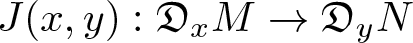 $J(x,y):\mathfrak{D}_xM\to \mathfrak{D}_yN$ such that
 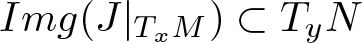 $Img(J|_{T_xM})\subset T_yN$ and
 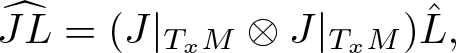 $\widehat{JL} = (J|_{T_xM}\otimes J|_{T_xM}) \hat{L},$ then this map
  $J(x,y)$ is called a Schwartz morphism and
  $J$ is a section of bundle of linear maps
 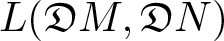 $L(\mathfrak{D}M,\mathfrak{D}N)$ on the manifold
  $M\times N$ that gives a Schwartz morphism at every point
  $(x,y)$, i.e.,
 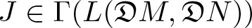 $J\in \Gamma(L(\mathfrak{D}M,\mathfrak{D}N))$ is a field of Schwartz morphisms. In this article, although sometimes we may refer to
  $J$ as the Schwartz morphism, one must remember that
  $J$ is, in fact, a field of Schwartz morphisms. As per Schwartz’s stochastic differential geometric approach, an SDE for a process
  $X_t$ on a manifold
  $M$ is defined as
 \begin{equation}
\mathbf{d}X_t = J(Y_t,X_t)\mathbf{d}Y_t,
\end{equation}
\begin{equation}
\mathbf{d}X_t = J(Y_t,X_t)\mathbf{d}Y_t,
\end{equation} where  $J$ is a Schwartz morphism from manifold
  $N$ to manifold
  $M$, and
  $Y_t$ is a given semimartingale on the manifold
  $N$. This equation is known as Schwartz SDE.
In order to represent a semimartingale on  $M$ in terms of a Schwartz SDE, we need a semimartingale on some manifold
  $N$ and a Schwartz morphism from manifold
  $N$ to
  $M$. If we consider
  $N$ as Euclidean with
  $Y_t$ as a semimartingale on
  $N$, then the problem remains to find the Schwartz morphism from
  $N$ to
  $M$. The following well-known theorem states that if we have a smooth map
  $\phi:N\to M$, then the Schwartz morphism from
  $N$ to
  $M$ is given by the diffusion map
  $\mathfrak{D}\phi$. The reader can refer to [Reference Émery2] for the proof of the theorem.
Theorem 1.1 ([Reference Émery2])
If 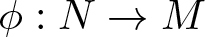 $\phi:N\to M$ is a smooth map, then the diffusion map
 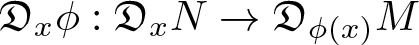 $\mathfrak{D}_{x}\phi:\mathfrak{D}_xN\to \mathfrak{D}_{\phi(x)}M$ is a Schwartz morphism from point
  $x$
$x$  $\to$
$\to$  $\phi(x)$. Moreover, if
  $U_t$ is a semimartingale on
  $N$, then the semimartingale
  $\phi(U_t)$ on
  $M$ is given by the solution of the Schwartz SDE,
 \begin{equation}
\textbf{d}X_t = \mathfrak{D}_{U_t}\phi(\textbf{d}U_t).
\end{equation}
\begin{equation}
\textbf{d}X_t = \mathfrak{D}_{U_t}\phi(\textbf{d}U_t).
\end{equation} In other words, the Schwartz differential  $\textbf{d}(\phi(U_t))$ is obtained by the push forward of the Schwartz differential
  $\textbf{d}U_t$ by
  $\phi$; i.e.,
 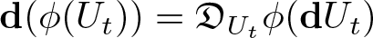 $\textbf{d}(\phi(U_t)) = \mathfrak{D}_{U_t}\phi(\textbf{d}U_t)$.
According to the following theorem from [Reference Émery2], the Schwartz morphism can be constructed using the flow of differential equation defined using the linear map 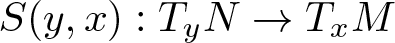 $S(y,x):T_yN\to T_xM$. The operator
  $S(y,x)$, is known as Stratonovich operator.
Theorem 1.2 ([Reference Émery2])
For every Stratonovich operator  $S(y,x):T_yN\to T_xM$, there exists a unique Schwartz operator
  $J(y,x):\mathfrak{D}_yN\to \mathfrak{D}_xM$, such that the Stratonovich SDE
  $\delta X_t = S(U_t,X_t)\delta U_t$ has the same solution as that of the Schwartz SDE
 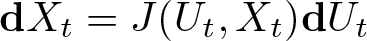 $\mathbf{d}X_t = J(U_t,X_t)\mathbf{d}U_t$; such that, for smooth curves
  $(x(t),y(t))\in M\times N$, if
  $ \dot{x}(t) = S(y(t),x(t))\dot{y}(t)$, then
 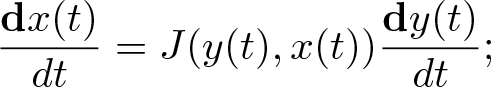 $\dfrac{\mathbf{d}x(t)}{dt} = J(y(t),x(t)) \dfrac{\mathbf{d}y(t)}{dt};$ where
  $\dfrac{\mathbf{d}c(t)}{dt}$ for some curve
  $c(t)$ is given by
  $\dfrac{\mathbf{d}c(t)}{dt}= \mathfrak{D}c\left(\dfrac{d^2}{dt^2}\right)$.
Let us consider an arbitrary Schwartz morphism 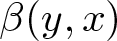 $\beta(y,x)$ from
  $\mathbb{R}^{p+1}$ to
  $M$ that does not have an explicit dependence on
  $y$. We know that, locally on the chart
  $(U,\chi)$, such a Schwartz morphism is given by
 \begin{equation*}\beta(y,x) L|_U = \left( f^i_l(x) a^l + g^i_{lm}(x)b^{lm}\right) \partial_i + \left(f^i_l(x) f^j_m(x) b^{lm} \right) \partial^2_{ij},\end{equation*}
 for every  $L \in \mathfrak{D}_y\mathbb{R}^{p+1}$ such that
  $L = a^l\partial_l + b^{lm}\partial^2_{lm}$ and the indices
  $l,m \in \{0,1, 2, ..., p\}$. Here,
  $f^i_l, g^i_{lm}$ are local coefficients of
  $\beta$. With this Schwartz morphism
  $\beta$, if we consider the SDE
 \begin{equation*}\mathbf{d}X_t = \beta(X_t) \mathbf{d}(t,W_t),\end{equation*}
then we find that
 \begin{equation}
\begin{aligned}
\mathbf{d}X_t|_U =\left[ f^i_0(X_t)\partial_i +\dfrac{1}{2}\left( \sum_{l=1}^p g^i_{ll}(X_t)\partial_i +(f^i_l(X_t) f^j_l(X_t))\partial^2_{ij}\right)\right] dt\\ + \sum_{l=1}^p(f^i_l(X_t) \partial_i)dW^l_t.
\end{aligned}
\end{equation}
\begin{equation}
\begin{aligned}
\mathbf{d}X_t|_U =\left[ f^i_0(X_t)\partial_i +\dfrac{1}{2}\left( \sum_{l=1}^p g^i_{ll}(X_t)\partial_i +(f^i_l(X_t) f^j_l(X_t))\partial^2_{ij}\right)\right] dt\\ + \sum_{l=1}^p(f^i_l(X_t) \partial_i)dW^l_t.
\end{aligned}
\end{equation} Note that the term in parentheses with coefficient  $\dfrac{1}{2}$ transforms as a diffusor if
  $f^i_0\partial_i, f^i_l\partial_i$ are local representations of vector fields. Therefore, if we consider vector fields
  $V,\sigma_1, ..., \sigma_p\in \mathfrak{X}(M)$, and a diffusor field
  $\alpha\in \Gamma(\mathfrak{D}M)$; then the following equation,
 \begin{equation}
\mathbf{d}X_t = Vdt +\dfrac{1}{2}\alpha dt + \sum_{l=1}^p\sigma_ldW^l_t,
\end{equation}
\begin{equation}
\mathbf{d}X_t = Vdt +\dfrac{1}{2}\alpha dt + \sum_{l=1}^p\sigma_ldW^l_t,
\end{equation} is a co-ordinate invariant representation of equation (1.7) if the diffusor field  $\alpha$ is such that
 \begin{equation}
\widehat{\alpha} = \sum_{l=1}^p\sigma_l \otimes \sigma_l.
\end{equation}
\begin{equation}
\widehat{\alpha} = \sum_{l=1}^p\sigma_l \otimes \sigma_l.
\end{equation}Remark 1.3. Since we consider a Schwartz morphism 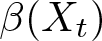 $\beta(X_t)$ that does not explicitly depend on the driving process
 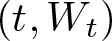 $(t,W_t)$, we end up with autonomous deterministic fields on the right-hand side of equation (1.8). Instead, one can also start with the Schwartz morphism
 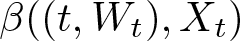 $\beta((t,W_t),X_t)$, which has an explicit dependence on
  $(t,W_t)$. In this case, one ends up with non-autonomous and adapted fields. In this article, we focus only on autonomous deterministic fields.
Based on Theorem 1.2, if we consider the Stratonovich differential equation
 \begin{equation*}\partial X_t = V(X_t) dt + \sum_{l = 1}^p\sigma_l(X_t) \circ dW^l_t,\end{equation*}
then it is easy to verify that the equivalent Schwartz SDE is
 \begin{equation*}\mathbf{d}X_t = \left[V(X_t) + \dfrac{1}{2}\alpha_S(X_t) \right] dt + \sum_{l = 1}^p\sigma_l(X_t) dW^l_t,\end{equation*}
 where  $\alpha_S$ is locally given as
 \begin{equation*}\alpha_S|_U = \sum_{l = 1}^pd\sigma^i_l\cdot\sigma_l\dfrac{\partial}{\partial x^i} + \sum_{l = 1}^p\sigma^i_l \sigma^j_l\dfrac{\partial^2}{\partial x^i \partial x^j}.\end{equation*}
 From [Reference Émery1], we know that the following short exact sequence is valid at every point  $x\in M$.

This implies that there exists an isomorphism  $J_x:\mathfrak{D}_xM\to T_xM \oplus (T_xM\odot T_xM)$. Moreover, if we represent a linear map from
  $\mathfrak{D}_xM$ to
  $T_xM$ as
  $Q_x$, then
 \begin{equation}
J_x(\cdot) = (Q_x(\cdot), \widehat{\cdot}).
\end{equation}
\begin{equation}
J_x(\cdot) = (Q_x(\cdot), \widehat{\cdot}).
\end{equation} In chapter 7 of [Reference Émery2], it has been demonstrated that such linear maps  $Q_x$ can be uniquely identified with a connection on the manifold. Therefore, from equation (1.10), it is possible to construct the isomorphism
  $J_x$ using a connection on the manifold. Due to the isomorphism
  $J_x$, a diffusor field
  $\lambda$ can be obtained from a vector field
  $V$ by considering
 \begin{equation*}\lambda_x = J_x^{-1}((Q_x(\lambda_x),V_x\otimes V_x)),\end{equation*}
 where  $Q_x:\mathfrak{D}_xM\to T_xM$ is the linear map corresponding to the given connection. If
  $\Gamma$ is the Christoffel symbol for the connection, then the diffusor field
  $\lambda$ is locally given as
 \begin{equation*}\lambda|_U = -\Gamma^i_{jk}V^jV^k\partial_i + V^iV^j\partial^2_{ij}.\end{equation*}
 Therefore, we find that there exists a diffusor field  $\alpha_I$ such that it is locally given as
 \begin{equation*}\alpha_I|_U = \sum_{l=1}^p -\Gamma^i_{jk}\sigma^j_l\sigma^k_l\partial_i + \sum_{l=1}^p\sigma^i_l \sigma^j_l\partial^2_{ij}.\end{equation*}
 Since 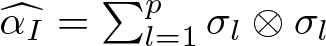 $\widehat{\alpha_I} = \sum_{l=1}^p\sigma_l \otimes \sigma_l$, the following SDE gives us a special case of equation (1.8),
 \begin{equation}
\mathbf{d}X_t = Vdt +\dfrac{1}{2}\alpha_I dt + \sum_{l=1}^p\sigma_ldW^l_t.
\end{equation}
\begin{equation}
\mathbf{d}X_t = Vdt +\dfrac{1}{2}\alpha_I dt + \sum_{l=1}^p\sigma_ldW^l_t.
\end{equation} Such equations are called Itô SDEs on manifolds. This idea of using a connection to construct a diffusor field  $\alpha$ (as given in equation (1.8)) was originally presented by Meyer in [Reference Meyer23] (in French). As English speakers, we find chapters 6 and 7 of [Reference Émery2] a useful reference. A modern approach that uses the idea of connections and the Itô-bundle can be found in [Reference Gliklikh14].
1.1.2. Basic Lagrangian mechanics
Now we will review some basics of Lagrangian mechanics, which will be used later in Section 3. For continuity, one may skip this section and return while reading Section 3. The reader may also refer to [Reference Abraham and Marsden3] for a complete introduction to various concepts in mechanics.
A smooth function  $L\in\mathfrak{F}(TM)$ on the tangent bundle of the manifold
  $M$ is called a Lagrangian. For a Lagrangian
  $L\in \mathfrak{F}(TM)$, the Euler–Lagrange equation for
  $c(t) \in TM$ is locally given as
 \begin{equation*}\dfrac{d}{dt}D_{\dot{x}}L((x(t),\dot{x}(t))) = D_xL((x(t),\dot{x}(t))),\end{equation*}
 where  $(x(t),\dot{x}(t))$ is the local representation of the curve
  $c(t)$. Fibre derivative of a Lagrangian
  $L$ is defined as a fibre-preserving map
  $FL: TM\to T^*M$ from tangent bundle to cotangent bundle over identity, such that if
  $L_x$ is the restriction of
  $L$ to the fibre at
  $x\in M$, then
 \begin{equation*}FL(v_x) = DL_x(v_x),\end{equation*}
 where  $DL_x(v_x)$ is the derivative of
  $L_x$ at point
  $v_x\in T_xM$. A Lagrangian
  $L\in \mathfrak{F}(TM)$ whose fibre derivative
  $FL$ is regular at all the points in
  $TM$ is called a regular Lagrangian. The canonical symplectic form on the cotangent bundle
  $T^*M$ is defined as a non-degenerate and closed differential 2-form
  $\omega_0\in \Omega^2(T^*M)$ such that
 \begin{equation*} \omega_0 = -d\theta;\end{equation*}
 where  $\theta\in \Omega^1(T^*M)$ such that
 \begin{equation*}\theta_\alpha(\beta) = \alpha\cdot T\tau^*_M(\beta),\end{equation*}
  $\forall$
  $\alpha\in T^*M$ and
  $\beta\in T_\alpha(T^*M)$. Using the fibre derivative of a Lagrangian, it is possible for us to define another function on
  $TM$, called energy. The energy
  $E\in \mathfrak{F}(TM)$ is defined as
 \begin{equation*}E(v) = FL(v)\cdot v - L(v) \ \text{for all } v\in TM.\end{equation*}
 The fibre derivative of a Lagrangian  $L$ also allows us to take the pullback of the canonical symplectic form
  $\omega_0$. For a regular Lagrangian, this pullback gives us
  $\omega_L = FL^*\omega_0$, which is a non-degenerate and closed differential 2-form on
  $TM$. Therefore,
  $\omega_L\in \Omega^2(TM)$ is symplectic and is called the Lagrangian symplectic form. A vector field
  $X_E\in \mathfrak{X}(TM)$ that satisfies
  $\mathbf{i}_{X_E}\omega_L= dE$ is called a Lagrangian vector field. In other words, the Lagrangian vector field is given as
  $X_E = \omega^\sharp_LdE$. Moreover, if
  $\dot{z} = X_E(z)$, then
  $E(z(t))$ is constant in time as
  $dE(z(t)) = dE\cdot \dot{z} = dE\cdot \omega^\sharp_LdE = 0$. Therefore, the flow of the Lagrangian vector field,
  $X_E$, is energy-preserving.
Theorem 1.4 ([Reference Abraham and Marsden3])
If  $X_E\in \mathfrak{X}(TM)$ is a Lagrangian vector field for a regular Lagrangian
  $L\in \mathfrak{F}(TM)$, then
  $X_E$ is necessarily a second-order vector field (i.e.,
  $(d/dt)(\tau_M\circ c)(t) = c(t)$ for all integral curves
  $c:I\to TM$ of
  $X_E$), which further implies that
  $X_E$ satisfies the Euler–Lagrange equation for the Lagrangian
  $L$.
$L$.
1.2. Motivation and detailed overview of the article
As seen in Section 1.1.1, there are two ways of constructing the diffusor field  $\alpha$ in equation (1.8). In the first approach, one considers the theorem 1.2 to obtain the diffusor field
  $\alpha_S$ that gives the Schwartz representation of the Stratonovich SDE. Another approach is to consider the Itô diffusor field
  $\alpha_I$, which requires a connection on the manifold. These two approaches are well known and well studied.
In this article, our interest is in the general way of constructing the diffusor field  $\alpha$ in the equation (1.8), without using the notion of connection and without depending on the underlying Stratonovich morphism. To this end, we observe that if the diffusor field
  $\alpha$ is considered to be a sum of diffusor fields
  $\alpha_l$ (i.e.,
  $\alpha = \sum_{l=1}^p \alpha_l$), such that for each
  $\alpha_l\in \Gamma(\mathfrak{D}M)$
 \begin{equation}
\widehat{\alpha_l} = \sigma_l \otimes \sigma_l,
\end{equation}
\begin{equation}
\widehat{\alpha_l} = \sigma_l \otimes \sigma_l,
\end{equation}then equation (1.8) changes to
 \begin{equation}
\mathbf{d}X_t = Vdt + \sum_{l=1}^p \left(\dfrac{1}{2}\alpha_l dt + \sigma_ldW^l_t\right).
\end{equation}
\begin{equation}
\mathbf{d}X_t = Vdt + \sum_{l=1}^p \left(\dfrac{1}{2}\alpha_l dt + \sigma_ldW^l_t\right).
\end{equation} As each  $\alpha_l$ has the property that
  $\widehat{\alpha_l} = \sigma_l \otimes \sigma_l$, each diffusor field
  $\alpha_l$ is associated with the vector field
  $\sigma_l$.
Due to this property of the diffusor field  $\alpha_l$, which requires the noise vector field
  $\sigma_l$, it is natural to ask if we can construct a diffusor from a given vector. To achieve this, we need a function that maps from the tangent space
  $T_xM$ to the diffusion space
  $\mathfrak{D}_xM$. In other words, we need a fibre-preserving map from
  $TM$ to
  $\mathfrak{D}M$ over identity.
Therefore, if we have a fibre-preserving map  $G: TM \to \mathfrak{D}M$ over identity, then a diffusor field
  $\alpha_l$ can be obtained from a vector field
  $\sigma_l$ by considering
 \begin{equation*}\alpha_l(x) = G(\sigma_l(x)) \ \text{for all } x\in M.\end{equation*}
 As we have to ensure that  $\widehat{\alpha_l} = \sigma_l \otimes \sigma_l$, we must construct the function
  $G$ such that
 \begin{equation*}\widehat{G(v)} = v \otimes v\end{equation*}
 for all  $v\in TM$. Using such a function
  $G$, we can rewrite equation (1.8) as
 \begin{equation}
\mathbf{d}X_t = \left[V(X_t) + \dfrac{1}{2} \sum_{l = 1}^p G\circ\sigma_l(X_t)\right]dt + \sum_{l=1}^p \sigma_l(X_t) dW^l_t.
\end{equation}
\begin{equation}
\mathbf{d}X_t = \left[V(X_t) + \dfrac{1}{2} \sum_{l = 1}^p G\circ\sigma_l(X_t)\right]dt + \sum_{l=1}^p \sigma_l(X_t) dW^l_t.
\end{equation} We have already seen an example of this function  $G$ in the case of Itô SDE representation, where
 \begin{equation*}G(v)|_U = \alpha_I|_U = -\Gamma^i_{jk}v^jv^k\partial_i + v^iv^j\partial^2_{ij}.\end{equation*}
 As discussed in the previous section, this was originally obtained by constructing a linear map  $Q_x:\mathfrak{D}_xM\to T_xM$ that depends on the given connection. However, this is just a special case of all possible functions
  $G$ and inevitably requires a connection.
Definition 1.5. We define a diffusion generator (or a type-I diffusion generator) as a fibre-preserving map 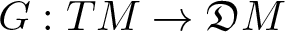 $G:TM\to \mathfrak{D}M$ over identity such that
 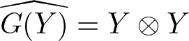 $\widehat{G(Y)} = Y\otimes Y$
  $\forall$
  $Y\in TM$. The set of all diffusion vector generators on the manifold
  $M$ will be denoted by
  ${\mathcal{G}(M)}$.
An equivalent definition for a map of fields is given as follows.
Definition 1.6. We define a diffusion field generator (or a type-II diffusion generator) as a map  $G:\mathfrak{X}(M)\to \Gamma(\mathfrak{D}M)$, such that
  $\widehat{G(\sigma)} = \sigma\otimes \sigma$
  $\forall$
  $\sigma\in\mathfrak{X}(M)$. The set of all diffusion field generators on the manifold
  $M$ will be denoted by
  ${\mathfrak{G}(M)}$.
Remark 1.7. Let  $G \in \mathcal{G}(M)$ be a smooth diffusion generator. This induces a map
 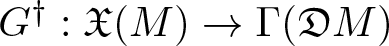 $G^\dagger:\mathfrak{X}(M)\to \Gamma(\mathfrak{D}M)$ such that
 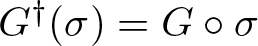 $ G^\dagger(\sigma)=G\circ\sigma$, for all
  $\sigma\in\mathfrak{X}(M)$. Since
 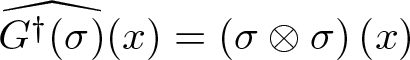 $\widehat{G^\dagger(\sigma)}(x)=\left(\sigma\otimes\sigma\right)(x)$ for all
  $x\in M$, the map
  $G^\dagger$ is in fact a diffusion field generator. In this work, as seen in equation (1.14), for SDEs on manifolds, we restrict our attention to fields as inputs to diffusion generators of both types. Consequently, as shown above, since a smooth diffusion generator (type-I diffusion generator) induces a diffusion field generator (type-II diffusion generator), it is not necessary to distinguish between type-I and type-II diffusion generator. Hence, we shall collectively refer to the maps of both types as diffusion generators, unless explicitly needed.
If a diffusion field generator is local then it induces a map between the space of germs of vector fields and the space of germs of diffusor fields.
Diffusion generator should not be confused with the generator of a stochastic process. However, given a noise vector field  $\sigma$, a diffusion generator can be identified with a generator of a semimartingale driven by a one-dimensional Wiener process. This identification is evident if we consider the equation
  $\mathbf{d}Z_t = \left[(G\circ\sigma)(Z_t)\right]dt/2 + \sigma(Z_t) dW_t$, wherein the generator for
  $Z_t$ is
 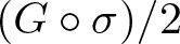 $(G\circ\sigma)/2$.
Some fundamental questions on the existence of a diffusion generator and its properties remain unanswered. In Section 2, we are mainly interested in exploring the construction of such maps. At the beginning of Section 2, we formally demonstrate that it is possible to construct a Schwartz morphism using a diffusion generator and a set of vector fields. Like Schwartz’s approach, the diffusion generator approach also generalizes the Stratonovich representation and the Itô representation of SDEs. This is demonstrated in Section 2.2 by constructing diffusion generators using the flow of differential equations. We observe that when the diffusion generator is obtained by considering the flow of first-order vector field, we end up with the Schwartz representation of the Stratonovich SDE. Similarly, when the diffusion generator is obtained using the geodesic equation, the corresponding SDE is nothing but the Itô SDE.
In [Reference Lázaro-Camí and Ortega21], one finds that a Hamiltonian (or a collection of Hamiltonians) allows one to describe a special type of Stratonovich SDE on the given manifold, and this equation is termed the stochastic Hamiltonian system. Using the symplectic form  $\omega_L$ on
  $TM$ given by a regular Lagrangian
  $L$, one can easily construct a stochastic Lagrangian system on
  $TM$ that preserves the energy of the system. However, exploring stochastic Hamiltonian/Lagrangian systems is not within the scope of this manuscript. Instead, we construct a canonical diffusion generator that is associated with a regular Lagrangian. We call this canonical diffusion generator as the Lagrangian diffusion generator. This is the second part of the article and can be found in Section 3.
An interesting application involving the stochastic Lagrangian system is in obtaining a stochastically varying vector field on  $M$ such that the motion of a stochastic point
  $X_t\in M$, described on the velocity phase space
  $TM$, is energy preserving. Let us assume that we are given a regular Lagrangian
  $L\in \mathfrak{F}(TM)$ such that the corresponding energy is given by
  $E\in \mathfrak{F}(TM)$. We are looking for a stochastic curve
  $Z_t\in TM$ such that
  $E(Z_t)$ is constant in time and
  $X_t = \tau_M\circ Z_t$. Clearly, if the stochastic process
  $Z_t\in TM$ is given by
 \begin{equation*}\delta Z_t = \omega^\sharp_L dE dt + \sum_{l = 1}^p \sigma_l \delta W^l_t,\end{equation*}
 where  $\sigma_l\in Ker(dE)$; then
  $\delta(E(Z_t)) = 0$, i.e., the energy of the system is constant.
As 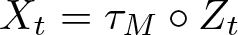 $X_t = \tau_M\circ Z_t$,
 \begin{equation*}\delta X_t = T\tau_M \delta Z_t = T\tau_M\omega^\sharp_L dE(Z_t) dt + \sum_{l = 1}^p T\tau_M\sigma_l(Z_t) \delta W^l_t\end{equation*}
 \begin{equation*} = Z_t dt + \sum_{l = 1}^p T\tau_M \sigma_l(Z_t) \delta W^l_t.\end{equation*}
 The question we are interested in answering is that if there exists a stochastically varying vector field  $F_t(x)\in T_xM$, then what is the SDE for
  $F_t(x)$ such that
 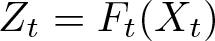 $Z_t = F_t(X_t)$?
If such a stochastically varying vector field  $F_t$ were to exist, then it would allow us to describe the energy preservation in terms of position
  $X_t$ and stochastically varying vector field
  $F_t(x)\in T_xM$. The existence of such a vector field
  $F_t$ is beyond the scope of this article, and we are only interested in finding the SDE representation of such a vector field
  $F_t(x)$. To answer this question, we need the generalized Itô formula that gives the SDE representation for the composition of the stochastic process
  $X_t$ into the stochastic field
  $F_t$. In the last part of this article (Section 4), we give the generalized Itô formula in terms of the diffusion generators.
2. Intrinsic stochastic differential equations using diffusion generators
Lemma 2.1. For vector fields  $V\in \mathfrak{X}(M)$,
  $\sigma_i\in \mathfrak{X}(M)$ for
  $i \in \{1, 2, ..., p\}$, and a diffusion generator
  $G\in \mathcal{G}(M)$, there exists a Schwartz morphism
 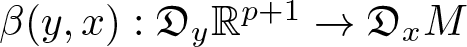 $\beta(y,x):\mathfrak{D}_y\mathbb{R}^{p+1} \to \mathfrak{D}_xM$ such that
 \begin{equation*}\beta((t,W_t),x) \mathbf{d}(t,W_t) = \left[V(x) + \dfrac{1}{2} \sum_{l = 1}^p G(\sigma_l(x))\right]dt + \sum_{l=1}^p \sigma_l(x) dW^l_t.\end{equation*}
Proof. Given vector fields  $V\in \mathfrak{X}(M)$,
  $\sigma_i\in \mathfrak{X}(M)$ for
  $i \in \{1, 2, ..., p\}$, and a diffusion generator for vector
  $G\in \mathcal{G}(M)$ such that
 \begin{equation*}G(v)|_U = g^i(v)\partial_i + v^iv^j\partial^2_{ij};\end{equation*}
 we can consider the Schwartz morphism  $\beta(y,x):\mathfrak{D}_y\mathbb{R}^{p+1} \to \mathfrak{D}_xM$ such that locally it is given as
 \begin{equation}
\begin{aligned}
\beta(y,x) L|_U & = \left( V^i(x) a^0 + \sigma^i_l(x) a^l + \sum_{n = 1}^p \dfrac{1}{p} g^i(\sigma_n(x))\delta_{lm}b^{lm}\right) \partial_i\\
& + \left(V^i\sigma^j_m(x)b^{0m} + \sigma^i_mV^jb^{m0} + V^iV^jb^{00} + \sigma^i_l(x) \sigma^j_m(x) b^{lm} \right) \partial^2_{ij},
\end{aligned}
\end{equation}
\begin{equation}
\begin{aligned}
\beta(y,x) L|_U & = \left( V^i(x) a^0 + \sigma^i_l(x) a^l + \sum_{n = 1}^p \dfrac{1}{p} g^i(\sigma_n(x))\delta_{lm}b^{lm}\right) \partial_i\\
& + \left(V^i\sigma^j_m(x)b^{0m} + \sigma^i_mV^jb^{m0} + V^iV^jb^{00} + \sigma^i_l(x) \sigma^j_m(x) b^{lm} \right) \partial^2_{ij},
\end{aligned}
\end{equation} for every  $L \in \mathfrak{D}_y\mathbb{R}^{p+1}$ such that
  $L = a^k\partial_k + b^{kz}\partial^2_{kz}$ and the indices
  $k,z \in \{0,1, 2, ..., p\}$ and
  $l,m \in \{1, 2, ..., p\}$. Clearly, this Schwartz morphism is constructed using the local components of the vector fields and the diffusion generator. It can be verified that
  $\beta((t,W_t),x) \mathbf{d}(t,W_t)$ is locally given as
 \begin{equation*}
\begin{split}
\beta((t,W_t),x) \mathbf{d}(t,W_t)|_U & = \left[\dfrac{1}{2} \sum_{l = 1}^p g^i(\sigma_l(x))\partial_i + \sigma^i_l(x)\sigma^j_l(x)\partial^2_{ij}\right]dt\\
& \quad+ V^i(x)\partial_i dt+ \sum_{l=1}^p \sigma^i_l(x)\partial_i dW^l_t\\
&= \left[V(x)|_U + \dfrac{1}{2} \sum_{l = 1}^p G(\sigma_l(x))|_U\right]dt + \sum_{l=1}^p \sigma_l(x)|_U dW^l_t.
\end{split}
\end{equation*}
\begin{equation*}
\begin{split}
\beta((t,W_t),x) \mathbf{d}(t,W_t)|_U & = \left[\dfrac{1}{2} \sum_{l = 1}^p g^i(\sigma_l(x))\partial_i + \sigma^i_l(x)\sigma^j_l(x)\partial^2_{ij}\right]dt\\
& \quad+ V^i(x)\partial_i dt+ \sum_{l=1}^p \sigma^i_l(x)\partial_i dW^l_t\\
&= \left[V(x)|_U + \dfrac{1}{2} \sum_{l = 1}^p G(\sigma_l(x))|_U\right]dt + \sum_{l=1}^p \sigma_l(x)|_U dW^l_t.
\end{split}
\end{equation*}Since this is true for all the charts, the proof is complete.
Before proving the converse of the above lemma, let us consider the following property of the diffusion generators.
Lemma 2.2. Consider  $n$ diffusion generators
  $G_i\in \mathcal{G}(M)$ for
  $i\in \{1, ..., n\}$. The average of all these diffusion generators
  $\left\langle G_i\right\rangle$, defined as
 \begin{equation*}\left\langle G_i\right\rangle = \dfrac{1}{n}\sum_{i = 1}^n G_i,\end{equation*}
is also a diffusion generator.
Proof. To prove 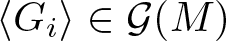 $\left\langle G_i\right\rangle\in \mathcal{G}(M)$, we need to prove that
  $\widehat{\left\langle G_i\right\rangle(X)} = X\otimes X$ for all
  $X\in TM$. But this is true because
  $\widehat{\left\langle G_i\right\rangle(X)} = \dfrac{1}{n}\sum_{i = 1}^n \widehat{G_i(X)}$ and
  $\widehat{G_i(X)} = X\otimes X$.
Lemma 2.3. Consider a field of Schwartz morphisms  $\beta$ from
  $\mathbb{R}^{p+1}$ to
  $M$ that does not explicitly depend on the driving process
  $(t,W_t)\in \mathbb{R}^{p+1}$. Let
  $(U,\chi)$ be a chart on
  $M$. Then there exists a 3-tuple
  $(V,\{\sigma_i\},G)$ of vector fields
  $V, \sigma_1, \sigma_2, ...,\sigma_p\in \mathfrak{X}(U)$, and a diffusion generator
  $G\in\mathcal{G}(U)$ such that for some semimartingale
  $X_t\in U\subset M$, given by
  $\mathbf{d}X_t=\beta(X_t) \mathbf{d}(t,W_t),$ we get
 \begin{equation}
\begin{aligned}
\mathbf{d}X_t|_U =\left[\beta(X_t) \mathbf{d}(t,W_t)\right]\big\vert_U &\\
= &\left[V(X_t) + \dfrac{1}{2} \sum_{l = 1}^p G(\sigma_l(X_t))\right]dt + \sum_{l=1}^p \sigma_l(X_t)dW^l_t.
\end{aligned}
\end{equation}
\begin{equation}
\begin{aligned}
\mathbf{d}X_t|_U =\left[\beta(X_t) \mathbf{d}(t,W_t)\right]\big\vert_U &\\
= &\left[V(X_t) + \dfrac{1}{2} \sum_{l = 1}^p G(\sigma_l(X_t))\right]dt + \sum_{l=1}^p \sigma_l(X_t)dW^l_t.
\end{aligned}
\end{equation}Proof. Following the discussion in Section 1.1, from equation (1.7) we know that locally,
 \begin{equation}
\begin{aligned}
\mathbf{d}X_t|_U =& \left[ f^i_0(X_t)\partial_i +\dfrac{1}{2}\left( \sum_{l=1}^p g^i_{ll}(X_t)\partial_i +(f^i_l(X_t) f^j_l(X_t))\partial^2_{ij}\right)\right] dt \\
&\qquad\qquad\qquad\qquad\qquad\qquad\qquad+ \sum_{l=1}^p(f^i_l(X_t) \partial_i)dW^l_t,
\end{aligned}
\end{equation}
\begin{equation}
\begin{aligned}
\mathbf{d}X_t|_U =& \left[ f^i_0(X_t)\partial_i +\dfrac{1}{2}\left( \sum_{l=1}^p g^i_{ll}(X_t)\partial_i +(f^i_l(X_t) f^j_l(X_t))\partial^2_{ij}\right)\right] dt \\
&\qquad\qquad\qquad\qquad\qquad\qquad\qquad+ \sum_{l=1}^p(f^i_l(X_t) \partial_i)dW^l_t,
\end{aligned}
\end{equation} where  $f^i_l, g^i_{lm}$ are local coefficients of
  $\beta$. Suppose that there exist a 3-tuple
  $(V,\{\sigma_i\},G)$ of vector fields
  $V, \sigma_1, \sigma_2, ...,\sigma_p\in \mathfrak{X}(U)$, and a diffusion generator
  $G\in\mathcal{G}(U)$ such that the statement of the lemma is satisfied. Then, we find that locally
 \begin{equation*}V = f^i_0\partial_i,\end{equation*}
 \begin{equation*}\sigma_l= f^i_l\partial_i,\text{and}\end{equation*}
 \begin{equation}
\sum_{l=1}^pG(\sigma_l(X_t)) = \sum_{m=1}^p g^i_{mm}(X_t)\partial_i + \sigma^i_m(X_t)\sigma^j_m(X_t)\partial^2_{ij}.
\end{equation}
\begin{equation}
\sum_{l=1}^pG(\sigma_l(X_t)) = \sum_{m=1}^p g^i_{mm}(X_t)\partial_i + \sigma^i_m(X_t)\sigma^j_m(X_t)\partial^2_{ij}.
\end{equation} Therefore, we need to prove that there exists such a diffusion generator  $G$ that satisfies the above equation (2.4). For this, we first define
  $p$ diffusion generators
  $G_m\in \mathcal{G}(U)$ for
  $m\in \{1,2, ..., p\}$ such that they are locally given as
 \begin{equation*}G_m(v) = g^i_{mm}\circ\tau_M(v) \partial_i + v^iv^j\partial^2_{ij}.\end{equation*}
 Then from the lemma 2.2, we know that the average of these diffusion generators 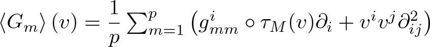 ${\left\langle G_m\right\rangle(v)} = \dfrac{1}{p}\sum_{m = 1}^p\left( g^i_{mm}\circ\tau_M(v) \partial_i + v^iv^j\partial^2_{ij}\right)$ is also a diffusion generator. If
 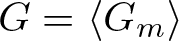 $G = \left\langle G_m\right\rangle$, then we find that
 \begin{equation*}G(\sigma_l(X_t)) = \dfrac{1}{p}\left(\sum_{m = 1}^p g^i_{mm}\circ\tau_M(\sigma_l(X_t)) \partial_i\right) + \sigma^i_l(X_t)\sigma^j_l(X_t)\partial^2_{ij}.\end{equation*}
 \begin{align*}
\therefore \sum_{l=1}^pG(\sigma_l(X_t)) = \sum_{l=1}^p\left[\dfrac{1}{p}\left( \sum_{m = 1}^p g^i_{mm}(X_t) \partial_i \right) + \sigma^i_l(X_t)\sigma^j_l(X_t)\partial^2_{ij}\right] \\
=\sum_{n=1}^p g^i_{nn}(X_t) \partial_i + \sigma^i_n(X_t)\sigma^j_n(X_t)\partial^2_{ij},
\end{align*}
\begin{align*}
\therefore \sum_{l=1}^pG(\sigma_l(X_t)) = \sum_{l=1}^p\left[\dfrac{1}{p}\left( \sum_{m = 1}^p g^i_{mm}(X_t) \partial_i \right) + \sigma^i_l(X_t)\sigma^j_l(X_t)\partial^2_{ij}\right] \\
=\sum_{n=1}^p g^i_{nn}(X_t) \partial_i + \sigma^i_n(X_t)\sigma^j_n(X_t)\partial^2_{ij},
\end{align*}which is nothing but equation (2.4).
With lemma 2.1 and lemma 2.3, we have formally demonstrated that the type-I diffusion generator serves as an alternative to the idea of Schwartz morphism when the driving process of the Schwartz SDE is  $(t,W_t)$. As discussed in remark 1.7, a smooth type-I diffusion generator induces a type-II diffusion generator. Therefore, these results easily extend to the case of type-II diffusion generator as well. This allows us to formally define what we mean by an Intrinsic SDE obtained using a diffusion generator.
Definition 2.4. We define an Intrinsic Stochastic Differential Equation using a diffusion generator as a 3-tuple  $(V,\{\sigma_i\}, G)$, where
  $V\in \mathfrak{X}(M)$,
  $\sigma_i\in \mathfrak{X}(M)$ for
  $i \in \{1, 2, ..., p\}$, and
 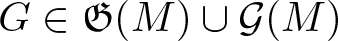 $G\in \mathfrak{G}(M)\cup \mathcal{G}(M)$. The Intrinsic SDE
 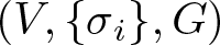 $(V,\{\sigma_i\}, G)$ can also be written in the form of equation (1.14)
 \begin{align*}
\mathbf{d}X_t = \left[V(X_t) + \dfrac{1}{2} \sum_{l = 1}^p G\circ\sigma_l(X_t)\right]dt + \sum_{l=1}^p \sigma_l(X_t) dW^l_t.
\tag{(1.14)}
\end{align*}
\begin{align*}
\mathbf{d}X_t = \left[V(X_t) + \dfrac{1}{2} \sum_{l = 1}^p G\circ\sigma_l(X_t)\right]dt + \sum_{l=1}^p \sigma_l(X_t) dW^l_t.
\tag{(1.14)}
\end{align*} A solution for the SDE  $(V,\{\sigma_i\}, G)$ is a semimartingale
  $X_t\in M$ that satisfies equation (1.14) in all the charts in the strong sense.
Notice that we allow both type-I and type-II diffusion generators in the above definition.
2.1. Existence and uniqueness of a local strong solution of an intrinsic SDE
We would like to see if equation (1.14) has a unique and strong solution that is adapted to the filtration generated by the Wiener process  $W_t\in \mathbb{R}^p$. We already know that equation (1.14) is just a reformulation of equation (1.8), and that equation (1.8) has a unique local (local in time) strong solution when the coefficients are smooth. In case the Intrinsic SDE is defined using a diffusion field generator, the existence of the local solution for the SDE is guaranteed because by definition, a diffusion field generator takes a smooth vector field as an input and outputs a smooth diffusor field. For the Intrinsic SDE with a type-I diffusion generator, we will need to ensure the smoothness for the existence of the solution.
Proposition 2.5. Given a smooth diffusion generator  $G\in \mathcal{G}(M)$, and smooth vector fields
  $V, \sigma_1, \sigma_2, ..., \sigma_p\in \mathfrak{X}(M),$ the Intrinsic SDE
 \begin{align*}
\mathbf{d}X_t = \left[V(X_t) + \dfrac{1}{2} \sum_{l = 1}^p G(\sigma_l(X_t))\right]dt + \sum_{l=1}^p \sigma_l(X_t) dW^l_t.
\tag{(1.14)}
\end{align*}
\begin{align*}
\mathbf{d}X_t = \left[V(X_t) + \dfrac{1}{2} \sum_{l = 1}^p G(\sigma_l(X_t))\right]dt + \sum_{l=1}^p \sigma_l(X_t) dW^l_t.
\tag{(1.14)}
\end{align*} has a unique local strong solution, i.e., there exists a semimartingale  $X_t\in M$ that satisfies the equation (locally in time) in the strong sense, for any initial condition
  $X_0\in M$.
Proof. Suppose for the vector field  $\sigma_l\in \mathfrak{X}(M)$, locally in the chart
  $(U,\chi)$ with coordinates
  $(x^1, x^2, ..., x^n)$,
  $\alpha_l = G(\sigma_l)$ is given as
 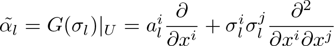 $\tilde{\alpha_l} = G(\sigma_l)|_U = a^i_l\dfrac{\partial}{\partial x^i} + \sigma^i_l \sigma^j_l \dfrac{\partial^2}{\partial x^i \partial x^j}$. In the chart
  $(U,\chi)$, the left-hand side of equation (1.14) is given by
 \begin{equation}
\mathbf{d}X_t|_U = dX^i_t\dfrac{\partial}{\partial x^i} +\dfrac{1}{2} d[X^i_t,X^j_t]\dfrac{\partial^2}{\partial x^i \partial x^j},
\end{equation}
\begin{equation}
\mathbf{d}X_t|_U = dX^i_t\dfrac{\partial}{\partial x^i} +\dfrac{1}{2} d[X^i_t,X^j_t]\dfrac{\partial^2}{\partial x^i \partial x^j},
\end{equation} where 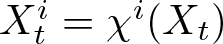 $X^i_t = \chi^i(X_t)$. Therefore, in chart
  $(U,\chi)$, we get the Itô SDEs,
 \begin{equation}
dX^i_t = (V^i+ \dfrac{1}{2}\sum_{l = 1}^p a^i_l)dt + \sigma^i_l dW^l_t
\end{equation}
\begin{equation}
dX^i_t = (V^i+ \dfrac{1}{2}\sum_{l = 1}^p a^i_l)dt + \sigma^i_l dW^l_t
\end{equation}and
 \begin{equation}
d[X^i_t,X^j_t] = \sigma^i_l(X_t)\sigma^j_l(X_t) dt.
\end{equation}
\begin{equation}
d[X^i_t,X^j_t] = \sigma^i_l(X_t)\sigma^j_l(X_t) dt.
\end{equation} The smoothness of the diffusor fields  $\alpha_l$ follows from the smoothness of the map
  $G$ and the smoothness of the vector fields
  $\sigma_l$. As the Itô SDE (2.6) has a unique local solution when the coefficients are smooth, we can conclude that if equation (1.14) is coordinate invariant, then there exists a unique semimartingale
  $X_t$ that satisfies equation (1.14) locally in time. As we already know that equation (1.14) is coordinate invariant, the proof is complete.
The notion of Intrinsic SDE using a diffusion generator can be easily generalized to the case with multiple diffusion generators  $G^1, G^2, ...,G^p\in \mathfrak{G}(M)\cup \mathcal{G}(M)$, in which the generic form with vector fields
  $V,\sigma_1, \sigma_2, ..., \sigma_p\in \mathfrak{X}(M)$ is given as
 \begin{equation}
\mathbf{d}X_t = \left[V(X_t) + \dfrac{1}{2} \sum_{l = 1}^p G^l\circ\sigma_l(X_t)\right]dt + \sum_{l=1}^p \sigma_l(X_t) dW^l_t.
\end{equation}
\begin{equation}
\mathbf{d}X_t = \left[V(X_t) + \dfrac{1}{2} \sum_{l = 1}^p G^l\circ\sigma_l(X_t)\right]dt + \sum_{l=1}^p \sigma_l(X_t) dW^l_t.
\end{equation}Like in the case of Intrinsic SDEs with a single diffusion generator, in the case of multiple diffusion generators, we need the diffusion generators of type-I to be smooth for the existence of a local, strong, and unique solution.
2.2. Construction of diffusion generators using flow of differential equations
From our review in Section 1.1, we know that

This implies that there exists an isomorphism  $J_x:\mathfrak{D}_xM\to T_xM \oplus (T_xM\odot T_xM)$. Therefore, if the isomorphism
 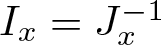 $I_x = J^{-1}_x$ is given, then a diffusion generator
  $G\in \mathfrak{G}(M)\cup\mathcal{G}(M)$ can be identified with a map
  $A_x:T_xM\to T_xM$ such that
 \begin{equation*}G(v_x) = I_x((A_x(v_x),v_x\otimes v_x)).\end{equation*}
 Therefore, the isomorphism  $I_x:\mathfrak{D}_xM\to T_xM \oplus (T_xM\odot T_xM)$ and the map
 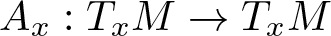 $A_x:T_xM\to T_xM$ can be used to define a diffusion generator. An example of a diffusion generator obtained through such construction is the case of a manifold with connection, which gives us an Itô SDE.
In this section, we will demonstrate that it is possible to obtain diffusion generators using the flow of differential equations as well. For this purpose, we consider the smooth curve  $c(t)$ with the diffusor
 \begin{equation*}\dfrac{\mathbf{d}c}{dt} = \mathfrak{Dc}\dfrac{d^2}{dt^2}.\end{equation*}
 We know that in chart  $(U,\chi)$,
 \begin{equation}
\dfrac{\mathbf{d}c}{dt}\Big\vert_{U} = \ddot{c}^i\partial_i + \dot{c}^i\dot{c}^j\partial^2_{ij}.
\end{equation}
\begin{equation}
\dfrac{\mathbf{d}c}{dt}\Big\vert_{U} = \ddot{c}^i\partial_i + \dot{c}^i\dot{c}^j\partial^2_{ij}.
\end{equation} Since  $\widehat{\dfrac{\mathbf{d}c}{dt}} = \dot{c}\otimes \dot{c}$, any function that maps the vector
  $\dot{c}$ to the diffusor
 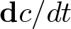 $\mathbf{d}c/dt$ should give us the diffusion generator. This approach of constructing a diffusion generator using smooth curves is similar to the 2-jet approach discussed in [Reference Armstrong and Brigo5]. This is because both approaches are fundamentally based on the idea of considering up to second derivative of the curve. In this section, we will only consider curves obtained through the flow of first-order and second-order differential equations.
2.2.1. Construction of diffusion generator using flow of first-order differential equation and its relation to Stratonovich SDEs
Recall from Section 1.1, if the vector field  $\sigma\in \mathfrak{X}(M)$ is taken as the noise coefficient in a Stratonovich SDE on a manifold
  $M$, then the associated diffusor field
  $\alpha_S\in \Gamma(\mathfrak{D}M)$ is such that locally, in chart
  $(U,\chi)$ with coordinates
  $(x^1, x^2, ..., x^n)$,
 \begin{equation}
\tilde{\alpha}_S = \alpha_S|_U = d\sigma^i\cdot\sigma\dfrac{\partial}{\partial x^i} + \sigma^i \sigma^j\dfrac{\partial^2}{\partial x^i \partial x^j},
\end{equation}
\begin{equation}
\tilde{\alpha}_S = \alpha_S|_U = d\sigma^i\cdot\sigma\dfrac{\partial}{\partial x^i} + \sigma^i \sigma^j\dfrac{\partial^2}{\partial x^i \partial x^j},
\end{equation} where  $\sigma^i = d\chi^i\cdot \sigma$. The fact that
  $\alpha_S\in \Gamma(\mathfrak{D}M)$ is indeed a diffusor field can be easily verified by checking the coordinate invariance. Moreover, the diffusor field
  $\alpha_S\in \Gamma(\mathfrak{D}M)$ is associated with the vector field
  $\sigma\in \mathfrak{X}(M)$. This association can be expressed through a diffusion field generator
  $G_S\in \mathfrak{G}(M)$ such that
 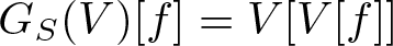 $G_S(V)[f] = V[V[f]]$, for all
  $f\in \mathfrak{F}(M)$ and
  $V\in \mathfrak{X}(M)$. The map is locally given as
 \begin{equation}
G_S(\sigma)|_U=d\sigma^i\cdot\sigma\dfrac{\partial}{\partial x^i} + \sigma^i \sigma^j\dfrac{\partial^2}{\partial x^i \partial x^j}.
\end{equation}
\begin{equation}
G_S(\sigma)|_U=d\sigma^i\cdot\sigma\dfrac{\partial}{\partial x^i} + \sigma^i \sigma^j\dfrac{\partial^2}{\partial x^i \partial x^j}.
\end{equation} Now, let us consider an alternative viewpoint. To each vector field  $\sigma\in \mathfrak{X}(M)$, we can associate a restricted type-I diffusion generator
  $G_{S,\sigma}\in \mathcal{G}(M)|_{Img(\sigma)}$ (as a map
  $G_{S,\sigma}:Img(\sigma)\to \mathfrak{D}(M)$ such that
  $\widehat{G}_{S,\sigma}(v) = v\otimes v$
  $\forall$
  $v\in Img(\sigma)\subset TM$). This map is locally given as
 \begin{equation}
G_{S,\sigma}(v)|_U = d\sigma^i\cdot v\dfrac{\partial}{\partial x^i} + v^i v^j\dfrac{\partial^2}{\partial x^i \partial x^j}, \forall v\in Img(\sigma).
\end{equation}
\begin{equation}
G_{S,\sigma}(v)|_U = d\sigma^i\cdot v\dfrac{\partial}{\partial x^i} + v^i v^j\dfrac{\partial^2}{\partial x^i \partial x^j}, \forall v\in Img(\sigma).
\end{equation} Because a point  $v\in Img(\sigma)\subset TM$ is given as
  $\sigma(x)\in TM$ for
  $x\in \tau_M(v)$, the diffusion field generator induced by the type-I restricted diffusion generator
  $G_{S,\sigma}$ (as per remark 1.7) is given as
 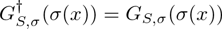 $G^\dagger_{S,\sigma}(\sigma(x)) = G_{S,\sigma}(\sigma(x))$. But, we observe that
  $G_{S,\sigma}(\sigma(x)) = G_S(\sigma)(x)$. Moreover, this is true for every vector field
  $\sigma\in\mathfrak{X}(M)$. In other words,
  $G_{S,\sigma}(\sigma(x)) = G_S(\sigma)(x)$ for all
  $\sigma\in \mathfrak{X}(M)$. Hence, even with the alternative viewpoint of restricted type-I diffusion generator, we ultimately end up with the diffusor field given by the diffusion field generator
  $G_S\in \mathfrak{G}(M)$.
In the proof of the following lemma, we show that the diffusion generator  $G_S\in \mathfrak{G}(M)$ is constructed through the flow of first-order differential equation and is related to Stratonovich SDEs.
Lemma 2.6. Let  $\sigma\in \mathfrak{X}(M)$ be a vector field on the manifold
  $M$. There exists a diffusion field generator
  $G_S\in \mathfrak{G}(M)$ (given by equation (2.11)), such that the solution of the ODE
  $\dot{x} = \sigma(x)$ is also the solution of the Schwartz differential equation
 \begin{equation}
\dfrac{\mathbf{d}x}{dt} = G_S\circ\sigma(x).
\end{equation}
\begin{equation}
\dfrac{\mathbf{d}x}{dt} = G_S\circ\sigma(x).
\end{equation} Moreover, the Stratonovich SDE,  $\delta X_t = V(X_t) dt + \sigma(X_t)\circ dW_t$ with some drift vector field
  $V\in \mathfrak{X}(M)$, has an equivalent Schwartz SDE that is given by
 \begin{equation}
\mathbf{d}X_t = \left[V(X_t) + \dfrac{1}{2}G_S\circ\sigma(X_t)\right]dt +\sigma(X_t)dW_t.
\end{equation}
\begin{equation}
\mathbf{d}X_t = \left[V(X_t) + \dfrac{1}{2}G_S\circ\sigma(X_t)\right]dt +\sigma(X_t)dW_t.
\end{equation}Proof. We know that for a curve  $x(t)\in M$,
 \begin{equation}
\dfrac{\mathbf{d}x(t)}{dt}\Big\vert_U =\ddot{x}^i(t)\partial_i + \dot{x}^i(t)\dot{x}^j(t)\partial^2_{ij}.
\end{equation}
\begin{equation}
\dfrac{\mathbf{d}x(t)}{dt}\Big\vert_U =\ddot{x}^i(t)\partial_i + \dot{x}^i(t)\dot{x}^j(t)\partial^2_{ij}.
\end{equation} Since  $\dot{x}(t) = \sigma(x(t))$, we get
 \begin{equation}
\dfrac{\mathbf{d}x}{dt}\Big\vert_U =d\sigma^i\cdot \sigma\partial_i + \sigma^i\sigma^j\partial^2_{ij}.
\end{equation}
\begin{equation}
\dfrac{\mathbf{d}x}{dt}\Big\vert_U =d\sigma^i\cdot \sigma\partial_i + \sigma^i\sigma^j\partial^2_{ij}.
\end{equation} From equation (2.11), we know that the right-hand side of equation (2.16) is also given by  $G_S(\sigma)|_U$, where the map
  $G_S\in \mathfrak{G}(M)$. Since, this is true for any chart, we get
 \begin{equation*}
\dfrac{\mathbf{d}x}{dt} = G_S(\sigma)(x).
\end{equation*}
\begin{equation*}
\dfrac{\mathbf{d}x}{dt} = G_S(\sigma)(x).
\end{equation*}From Section 1.1.1, we know that
 \begin{equation}
\delta X_t = V(X_t) dt + \sigma(X_t)\circ dW_t,
\end{equation}
\begin{equation}
\delta X_t = V(X_t) dt + \sigma(X_t)\circ dW_t,
\end{equation}has an equivalent Schwartz SDE that is given by
 \begin{equation}
\begin{aligned}
\mathbf{d}X_t &= \left[V(X_t) + \dfrac{1}{2}\alpha_S(X_t)\right]dt +\sigma(X_t)dW_t\\
&= \left[V(X_t) + \dfrac{1}{2}G_{S}\circ\sigma(X_t)\right]dt +\sigma(X_t)dW_t.
\end{aligned}
\end{equation}
\begin{equation}
\begin{aligned}
\mathbf{d}X_t &= \left[V(X_t) + \dfrac{1}{2}\alpha_S(X_t)\right]dt +\sigma(X_t)dW_t\\
&= \left[V(X_t) + \dfrac{1}{2}G_{S}\circ\sigma(X_t)\right]dt +\sigma(X_t)dW_t.
\end{aligned}
\end{equation}Notice that the above lemma is a special case of a more general result given by theorem 1.2 that allows the conversion of a generalized Stratonovich SDE into a Schwartz SDE. The above result is in terms of the idea of diffusion generators.
Definition 2.7. The diffusion generator  $G_{S}\in \mathfrak{G}(M)$ that ensures that the solution of the ODE
  $\dot{x}(t) = \sigma(x(t))$ is also the solution of the Schwartz differential equation
 \begin{equation}\dfrac{\mathbf{d}x(t)}{dt} = G_S\circ\sigma(x(t)),\end{equation}
will be called Stratonovich diffusion generator.
2.2.2. Construction of diffusion generator using flow of second-order differential equations and its relation to Itô SDEs
We will now construct a diffusion generator using the flow of second-order differential equation. A second-order differential equation is defined by a vector field  $Z$ on the tangent bundle
  $TM$ such that
  $T\tau_M\circ Z = Id_{TM}$. Therefore, every second-order vector field is locally given as
 \begin{equation*}Z((x,v)) = ((x,v),(v,Z_V(x,v)))\end{equation*}
 for all  $z = (x,v)\in TM$, where
  $Z_V(z)\in VTM$ with
  $VTM = Ker(T\tau_M)$ as the vertical bundle. As
  $x(t) = \tau_M(z(t))$,
 \begin{equation*}\dot{x}(t) = T\tau_M(z(t))\cdot \dot{z}(t) =T\tau_M(z(t))\cdot Z(z(t)) = z(t).\end{equation*}
 Therefore,  $\ddot{x}^i(t) = Z^i_V(z(t))$.
Lemma 2.8. For a given second-order differential equation  $Z\in \mathfrak{X}(TM)$, there exists a diffusion generator
  $G_{Z}\in \mathcal{G}(M)$ such that if
  $z(t)$ is the solution of the second-order differential equation
  $\dot{z} = Z(z)$, then
 \begin{equation}\dfrac{\mathbf{d}x}{dt} = G_{Z}(z(t)),\end{equation}
 where  $x(t) = \tau_M(z(t))$.
Proof. Since
 \begin{equation*}\dfrac{\mathbf{d}x}{dt}\Big\vert_{U} = \ddot{x}^i\partial_i + \dot{x}^i\dot{x}^j\partial^2_{ij},\end{equation*}
 \begin{equation*}\dfrac{\mathbf{d}x}{dt}\Big\vert_{U} = Z_V^i(z(t))\partial_i + z^i(t)z^j(t)\partial^2_{ij}.\end{equation*}
 Therefore, if  $x(t) = \tau_M(z(t))$,
  $\dot{z} = Z(z)$, and
 \begin{equation*}G_Z(v)|_U = Z_V^i(v)\partial_i + v^i v^j \partial^2_{ij};\end{equation*}
then
 \begin{equation*}\dfrac{\mathbf{d}x}{dt} = G_{Z}(z(t)).\end{equation*}
 In terms of the covariant derivative  $\nabla$, a second-order equation is given as
  $\nabla_{\dot{x}}\dot{x} = Y(x)$, for some
  $Y\in \mathfrak{X}(M)$. A special case is
  $Y = 0$, in which the solution curve is a geodesic and satisfies
 \begin{equation*}(\nabla_{\dot{x}}\dot{x})^i = \ddot{x}^i + \Gamma^i_{jk}\dot{x}^j\dot{x}^k = 0.\end{equation*}
 Using lemma 2.8, we can construct a diffusion generator associated with the geodesic equation. Given a connection on the manifold, in local coordinates  $(U,\chi)$, the diffusion generator for the geodesic equation is given as,
 \begin{equation}
G(\dot{x})|_U = \ddot{x}^i\partial_i + \dot{x}^i\dot{x}^j\partial^2_{ij}= -\Gamma^i_{jk}\dot{x}^j\dot{x}^k\partial_i + \dot{x}^i\dot{x}^j\partial^2_{ij}.
\end{equation}
\begin{equation}
G(\dot{x})|_U = \ddot{x}^i\partial_i + \dot{x}^i\dot{x}^j\partial^2_{ij}= -\Gamma^i_{jk}\dot{x}^j\dot{x}^k\partial_i + \dot{x}^i\dot{x}^j\partial^2_{ij}.
\end{equation}We find that the resulting Intrinsic SDE with the above diffusion generator corresponding to the geodesic equation, is the Schwartz representation of the Itô SDE on a manifold with a connection, as defined in [Reference Gliklikh14] and [Reference Émery2].
Definition 2.9. Let  $G_I\in\mathcal{G}(M)$ be a diffusion generator on the manifold
  $M$ such that the solution of the differential equation
  $\nabla_{\dot{x}}\dot{x} = 0$ is also the solution of the Schwartz equation
  $\mathbf{d}x/dt = G_I(\dot{x})$. Then
  $G_I\in\mathcal{G}(M)$ will be called Itô diffusion generator. Locally, in chart
  $(U,\chi)$, an Itô diffusion generator for a manifold with a connection corresponding to the Christoffel form
  $\Gamma$ is given as
 \begin{equation}
G_I(v)|_U = -\Gamma_{ij}^k(x) v^iv^j\dfrac{\partial}{\partial x^i} + v^iv^j\dfrac{\partial^2}{\partial x^i \partial x^j},
\end{equation}
\begin{equation}
G_I(v)|_U = -\Gamma_{ij}^k(x) v^iv^j\dfrac{\partial}{\partial x^i} + v^iv^j\dfrac{\partial^2}{\partial x^i \partial x^j},
\end{equation} for all  $v\in TM$. We will call an SDE generated by
  $G_I$ as an Itô SDE.
Since  $\mathbf{d}x/dt = G_I(\dot{x})$ corresponds to the geodesic equation
  $\nabla_{\dot{x}}\dot{x} = 0$, the Itô diffusion generator is just another way to look at the geodesic spray. To construct the Itô diffusion generator (or the induced Itô SDE), the manifold must be equipped with a connection. In the following section, we show that if a regular Lagrangian is used to define a second-order equation, then the lemma 2.8 allows for the construction of a diffusion generator without using the notion of connection.
3. Construction of diffusion generator using Lagrangian
From theorem 1.4, we know that if we consider a regular Lagrangian  $L\in \mathfrak{F}(TM)$, then it is possible to construct a second-order vector field
  $X_E$. In Section 2.2, we have shown that one can construct a diffusion generator using the flow of both first-order and second-order vector fields. Therefore, by combining theorem 1.4 with the construction of the diffusion generator using the flow of a second-order vector field, we can obtain a diffusion generator using a regular Lagrangian.
The following proposition states the existence of a diffusion generator for every regular Lagrangian.
Proposition 3.1. For every regular Lagrangian  $L\in \mathfrak{F}(TM)$, there exists a diffusion generator
  $G_L\in \mathcal{G}(M)$ associated with the Lagrangian
  $L$ such that if
  $z(t)$ is the solution of the Hamiltonian dynamics
  $\dot{z} = \omega_L^\sharp dE$ (where
  $\omega_L = FL^*\omega_0$,
  $\omega_0$ is the canonical symplectic form on
  $T^*M$, and
  $E\in \mathfrak{F}(TM)$ such that
  $E(v) = FL(v)\cdot v - L(v)$), then
 \begin{equation}\mathbf{d}x/dt = G_L(z(t)),
\end{equation}
\begin{equation}\mathbf{d}x/dt = G_L(z(t)),
\end{equation} where  $x(t) = \tau_M(z(t))$. Moreover, locally in chart
  $(U,\chi)$,
 \begin{equation}
G_L(v)|_U = \left[A^{ij}(x,v)\left(\dfrac{\partial L}{\partial x^j} - \dfrac{\partial^2 L}{\partial x^k\partial \dot{x}^j}v^k \right)\right]\dfrac{\partial}{\partial x^i} + v^i v^j\dfrac{\partial^2}{\partial x^i \partial x^j}, \text{for all }v\in TM,
\end{equation}
\begin{equation}
G_L(v)|_U = \left[A^{ij}(x,v)\left(\dfrac{\partial L}{\partial x^j} - \dfrac{\partial^2 L}{\partial x^k\partial \dot{x}^j}v^k \right)\right]\dfrac{\partial}{\partial x^i} + v^i v^j\dfrac{\partial^2}{\partial x^i \partial x^j}, \text{for all }v\in TM,
\end{equation} where  $A$ is the inverse of the matrix
  $\left[D^2_{\dot{x},\dot{x}} L\right]$.
Proof. From theorem 1.4, we know that in the local coordinates, the solution of the second-order equation  $\dot{z} = \omega_L^\sharp dE$ with the initial condition
  $z(0) = (x_0,v_0)$ is equivalent to solution of the Euler–Lagrange equation
  $\dfrac{d}{dt}\dfrac{\partial L}{\partial \dot{x}^i} = \dfrac{\partial L}{\partial x^i}$ with the initial condition
  $x(0) = x_0$ and
  $\dot{x}(0) = v_0$. Since the Lagrangian is regular, the inverse of
  $\dfrac{\partial^2 L}{\partial \dot{x}^i \partial \dot{x}^j}$ exists (proposition 3.5.10 in [Reference Abraham and Marsden3]).
 \begin{equation}
\therefore \ddot{x}^i(t) = A^{ij}\left(\dfrac{\partial L}{\partial x^j}\Big\vert_{z(t)} - \dfrac{\partial^2 L}{\partial x^k\partial \dot{x}^j}\Big\vert_{z(t)}\dot{x}^k(t) \right),
\end{equation}
\begin{equation}
\therefore \ddot{x}^i(t) = A^{ij}\left(\dfrac{\partial L}{\partial x^j}\Big\vert_{z(t)} - \dfrac{\partial^2 L}{\partial x^k\partial \dot{x}^j}\Big\vert_{z(t)}\dot{x}^k(t) \right),
\end{equation} where  $A$ is the inverse of the matrix
  $\left[D^2_{\dot{x},\dot{x}} L\right]\Big\vert_{z(t)}$. From lemma 2.8, we know that if
  $G_L\in \mathcal{G}(M)$, such that locally in the chart
  $(U,\chi)$,
 \begin{equation}
G_L(v)|_U = \left[A^{ij}\left(\dfrac{\partial L}{\partial x^j}\Big\vert_{v} - \dfrac{\partial^2 L}{\partial x^k\partial \dot{x}^j}\Big\vert_{v}v^k \right)\right]\dfrac{\partial}{\partial x^i} + v^i v^j\dfrac{\partial^2}{\partial x^i \partial x^j},
\end{equation}
\begin{equation}
G_L(v)|_U = \left[A^{ij}\left(\dfrac{\partial L}{\partial x^j}\Big\vert_{v} - \dfrac{\partial^2 L}{\partial x^k\partial \dot{x}^j}\Big\vert_{v}v^k \right)\right]\dfrac{\partial}{\partial x^i} + v^i v^j\dfrac{\partial^2}{\partial x^i \partial x^j},
\end{equation} for all  $v\in T_xM$, then
 \begin{equation*}\mathbf{d}x/dt = G_L(z(t)),\end{equation*}
 where  $x(t) = \tau_M(z(t))$ and
  $z(t)$ is the solution of
  $\dot{z} = \omega_L^\sharp dE$.
Definition 3.2. Let  $G_L\in\mathcal{G}(M)$ be a diffusion generator such that the solution
  $z(t)$ of the Hamiltonian dynamics
 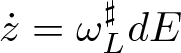 $\dot{z} = \omega_L^\sharp dE$ (where
  $L\in \mathfrak{F}(TM)$ is a regular Lagrangian,
  $\omega_L = FL^*\omega_0$,
  $\omega_0$ is the canonical symplectic form on
  $T^*M$, and
  $E\in \mathfrak{F}(TM)$ is the Energy, given as
  $E(v) = FL(v)\cdot v - L(v)$), also satisfies
  $\mathbf{d}x/dt = G_L(z(t))$, where
  $x(t) = \tau_M(z(t))$. Then
  $G_L\in\mathcal{G}(M)$ will be called Lagrangian diffusion generator. We will say that an SDE is generated by a Lagrangian
  $L$, if
  $G_L$ is the diffusion generator for the SDE.
In mechanics, one finds several interpretations of the equation of motion, such as the Symplectic formulation, the Poisson bracket formulation, the geodesic interpretation, and the interpretation using the calculus of variation [Reference Abraham and Marsden3]. All these interpretations yield the same equation of motion and usually require the Lagrangian. From the above definition, it is clear that using the Lagrangian diffusion generator, the solution to the Euler–Lagrange equation is also the solution to the Schwartz differential equation
 \begin{equation}
\dfrac{\mathbf{d}x}{dt} = G_L(\dot{x}(t)).
\end{equation}
\begin{equation}
\dfrac{\mathbf{d}x}{dt} = G_L(\dot{x}(t)).
\end{equation} Hence, using the Lagrangian diffusion generator, we have obtained the equation of motion through the diffusion bundle  $\mathfrak{D}{M}$ instead of the second tangent bundle
  $TTM$.
To understand the physical meaning of the Lagrangian diffusion generator in the context of SDEs, let us consider the general case of the diffusion generator obtained by using the flow of a second-order vector field  $Z\in \mathfrak{X}(TM)$. For this, we will consider the idea of the generator of an SDE. We know that for the Intrinsic SDE
 \begin{equation*}\mathbf{d}Y_t = \left[\dfrac{1}{2}(G_Z\circ\sigma)(Y_t)\right]dt + \sigma(Y_t) dW_t,\end{equation*}
 the generator for  $Y_t$ is
  $\dfrac{1}{2}(G_Z\circ\sigma)$. This means that in chart
  $(U,\chi)$,
 \begin{equation}
\lim_{\delta t\to 0^+}\dfrac{1}{\delta t}\mathbb{E}(Y^i_{t+\delta t} - Y^i_t) = \dfrac{1}{2}(G_Z\circ\sigma(Y_t))[\chi^i],
\end{equation}
\begin{equation}
\lim_{\delta t\to 0^+}\dfrac{1}{\delta t}\mathbb{E}(Y^i_{t+\delta t} - Y^i_t) = \dfrac{1}{2}(G_Z\circ\sigma(Y_t))[\chi^i],
\end{equation} where  $Y^i_t = \chi^i(Y_t)$. Moreover, we know that under the limit
  $\delta t\to 0^+$,
 \begin{equation*}Y^i_{t+\delta t} = Y^i_t + \dfrac{1}{2}(G_Z\circ\sigma)[\chi^i] \delta t + \sigma^i \mathcal{N} (0,\delta t),\end{equation*}
 satisfies the given SDE. Hence, the diffusion generator  $G_Z$, when composed with a vector
  $\sigma\in TM$, adds a drift in the direction
  $Z^i_V(\sigma)\partial_i$, the vertical part of
  $Z(\sigma)$. As the Lagrangian vector field
  $\omega_L^\sharp dE\in \mathfrak{X}(TM)$ is also a second-order vector field, the Lagrangian diffusion generator
  $G_L\in\mathcal{G}(M)$ adds a drift in the direction of the acceleration vector
 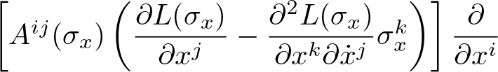 $\left[A^{ij}(\sigma_x)\left(\dfrac{\partial L(\sigma_x)}{\partial x^j} - \dfrac{\partial^2 L(\sigma_x)}{\partial x^k\partial \dot{x}^j}\sigma^k_x \right)\right]\dfrac{\partial}{\partial x^i}$, where
  $A$ is the inverse of the matrix
  $\left[D^2_{\dot{x},\dot{x}} L(\sigma_x)\right]$.
We will now consider some examples of the Lagrangian diffusion generator.
I. Manifold
$\mathbf{M}$ with a symmetric non-degenerate
$\mathbf{\mathcal{T}^0_2M}$ tensor-field
$\mathbf{\alpha}$. As
$\alpha\in T^0_2M$ is symmetric and non-degenerate, if
$L\in \mathfrak{F}(TM)$ such that
(3.7)\begin{equation}L(v) = \dfrac{1}{2}\alpha(v,v),\end{equation}for all
$v\in TM$, then from proposition 3.1 we obtain
(3.8)\begin{equation}
G_L(v)|_U = \left[\alpha^{ij}\left(\dfrac{1}{2}\dfrac{\partial \alpha_{lm}}{\partial x^j} v^lv^m - \dfrac{\partial \alpha_{jm}}{\partial x^k} v^kv^m \right)\right]\dfrac{\partial}{\partial x^i} + v^i v^j\dfrac{\partial^2}{\partial x^i \partial x^j}.
\end{equation}II. Riemannian manifold,
$\mathbf{(M,g)}$, with Kinetic energy as the Lagrangian. A special case of proposition 3.1, is a regular Lagrangian
$L\in \mathfrak{F}(TM)$ such that
(3.9)\begin{equation}L(v) = \dfrac{1}{2} g^\flat v\cdot v,\end{equation}where
$g$ is the Riemannian metric on the manifold
$M$. In Mechanics, such a Lagrangian is called Kinetic Energy. Moreover, if the initial state of the mechanical system is
$v\in TM$ and the solution is given by
$z(t)$, then
$x(t) = \tau_M(z(t))$ is a geodesic in the direction of
$v\in TM$, i.e.,
$x(t) = \exp_{\tau_M(v)}(vt) = \exp_{x_0}(\sigma(x_0)t).$From Riemannian geometry, it is known that
(3.10)\begin{equation}
\dfrac{d}{dt}\Big\vert_{t=0}(\exp_{\tau_M(v)}(vt)) = v
\end{equation}and, locally in chart
$(U,\chi)$,
(3.11)\begin{equation}
\dfrac{d^2}{dt^2}\Big\vert_{t=0}(\exp^k_{\tau_M(v)}(vt)) = \left\langle v,\nabla_v g^\sharp d\chi^k \right\rangle = -\Gamma_{ij}^k v^iv^j;
\end{equation}where
$\exp^k = \chi^k\circ \exp$. Hence, we can say that
$G\in \mathcal{G}(M)$ such that locally
(3.12)\begin{equation}
G(v)|_U = -\Gamma_{ij}^k v^iv^j\dfrac{\partial}{\partial x^i} + v^iv^j\dfrac{\partial^2}{\partial x^i \partial x^j}.
\end{equation}Comparing equation (3.12) with equation (2.22), we notice that this is a special case of diffusion generator constructed using connection obtained from the Riemannian metric. Hence, this is the Itô diffusion generator on the Riemannian manifold.
III. Riemannian manifold,
$\mathbf{(M,g)}$, with Kinetic energy - Potential Energy as the Lagrangian. Let
$\Phi:M\to R$ be the potential energy. Therefore, the Lagrangian is given by
$L\in\mathfrak{F}(TM)$ such that
(3.13)\begin{equation}L(v) = \dfrac{1}{2}g^\flat v\cdot v - \Phi(\tau_M(v)).\end{equation}Using proposition 3.1 we get
\begin{equation*}G_L(\sigma_x)|_U = \left[\left\lbrace\dfrac{\partial^2 L}{\partial \dot{x}^i \partial \dot{x}^j}\Big\vert_{(x,\sigma)}\right\rbrace^{-1}\left(\dfrac{\partial L}{\partial x^j}\Big\vert_{(x,\sigma)} - \dfrac{\partial^2 L}{\partial x^k\partial \dot{x}^j}\Big\vert_{(x,\sigma)}\sigma^k \right)\right]\dfrac{\partial}{\partial x^i}\end{equation*}(3.14)\begin{equation}+ \sigma^i \sigma^j\dfrac{\partial^2}{\partial x^i \partial x^j}.\end{equation}Therefore,
(3.15)\begin{equation}
\begin{aligned}
G_L(\sigma_x)|_U = g^{ij}(x)\left(\dfrac{\sigma^l}{2}\dfrac{\partial g_{lm}}{\partial x^j}(x)\sigma^m-\dfrac{\partial \Phi}{\partial x^j}(x) - \dfrac{\partial g_{jm}}{\partial x^k} \sigma^k\sigma^m\right)\dfrac{\partial}{\partial x^i}\\
+ \sigma^i \sigma^j\dfrac{\partial^2}{\partial x^i \partial x^j}.
\end{aligned}
\end{equation}In other words,
(3.16)\begin{equation}G_L(\sigma_x)|_U =\left( -\Gamma^i_{jk}\sigma^j\sigma^k -g^{ij}(x)\dfrac{\partial \Phi}{\partial x^j}(x)\right) \dfrac{\partial}{\partial x^i} + \sigma^i \sigma^j\dfrac{\partial^2}{\partial x^i \partial x^j}.
\end{equation}


4. Some equivalent representations and the extended Itô formula
The central theme of this section is the conversion of one form of an SDE into another. The idea of converting Schwartz SDE into Itô SDE/ Stratonovich SDE and vice versa is well known and has been considered in chapter 1 of [Reference Ferrucci13], where the author has shown that both Itô SDE and Stratonovich SDE can be reformulated as Schwartz SDE. In this section, we consider the representation conversion from the perspective of the diffusion generators.
One of the ways of representing the Itô SDEs is using the Belopolskya–Daletskii representation. From [Reference Gliklikh14], we know that the Belopolskya–Daletskii form for the Itô SDE 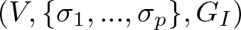 $\left(V,\{\sigma_1, ..., \sigma_p\}, G_I\right)$ is given by
 \begin{equation}
dX_t = \exp_{X_t}\left(V(X_t)dt + \sum_{l = 1}^p\sigma_l(X_t)dW^l_t\right),
\end{equation}
\begin{equation}
dX_t = \exp_{X_t}\left(V(X_t)dt + \sum_{l = 1}^p\sigma_l(X_t)dW^l_t\right),
\end{equation} where the exponential map  $\exp_x:T_xM\to M$ is due to the connection. In this section, we also show that we can convert an Intrinsic SDE with a diffusion generator into an equivalent Belopolskya–Daletskii type SDE. In order to obtain the Belopolskya–Daletskii form for the given Intrinsic SDE, we first convert the given Intrinsic SDE into an Itô SDE and then consider the Belopolskya–Daletskii form for the resulting Itô SDE.
In general, we derive a conversion formula to convert an Intrinsic SDE obtained using a diffusion generator into an Intrinsic SDE obtained using another diffusion generator. Furthermore, in Section 4.2, we use this conversion formula to derive the extended Itô formula on manifolds using the diffusion generator approach.
4.1. Equivalent representations of intrinsic SDEs in Itô representation, Stratonovich representation, and Belopolskya–Daletskii form
Earlier, in Section 3, we have observed that the Itô SDE
 \begin{equation*}\left(V,\{\sigma_1, ..., \sigma_p\}\right),\end{equation*}
is the same as the Intrinsic SDE
 \begin{equation*}\left(V,\{\sigma_1, ..., \sigma_p\}, G_I\right).\end{equation*}
 However, we do not know if an Intrinsic SDE with an arbitrary diffusion generator  $G$ can have an Itô representation. When written in the form of an equality, it is apparent that the Intrinsic SDE
 \begin{equation*}\left(V,\{\sigma_1, ..., \sigma_p\}, G\right)\end{equation*}
is the same as the Itô SDE
 \begin{equation*}\left(V + \dfrac{1}{2}\sum_{l = 1}^p (G(\sigma_l) - G_I(\sigma_l)),\{\sigma_1, ..., \sigma_p\}\right).\end{equation*}
 However, we need to prove that  $G(\sigma_l) - G_I(\sigma_l)$ is indeed a vector field.
Lemma 4.1. For every type-I diffusion generators  $G, G_\alpha \in \mathcal{G}(M)$, there exists a fibre preserving map
  $\nabla_\alpha^G:TM\to TM$ over identity such that
  $\nabla_\alpha^G(X) = G(X) - G_\alpha(X)$
  $\forall$
  $X\in TM$. Similarly, for every type-II diffusion generators
  $H,H_\alpha\in \mathfrak{G}(M)$, there exists a map
  $\nabla_\alpha^H:\mathfrak{X}(M)\to \mathfrak{X}(M)$ such that
  $\nabla_\alpha^H(\sigma) = H(\sigma) - H_\alpha(\sigma)$
  $\forall$
  $\sigma\in \mathfrak{X}(M)$.
Proof. As per the definition of the type-I diffusion generator, for any  $G\in \mathcal{G}(M)$,
 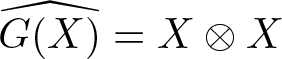 $\widehat{G(X)} = X\otimes X$,
  $\forall$
  $X\in TM$. Therefore,
 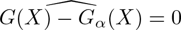 $\widehat{G(X)-G_\alpha(X)} = 0$, i.e.,
 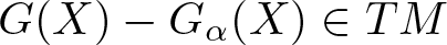 $G(X)-G_\alpha(X)\in TM$
  $\forall$
  $X\in TM$.
Similarly, we observe that for type-II diffusion generators  $H,H_\alpha\in \mathfrak{G}(M)$,
 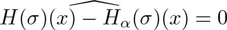 $\widehat{H(\sigma)(x) - H_\alpha(\sigma)(x)} = 0$ for all
  $\sigma\in \mathfrak{X}(M)$ and
  $x\in M$. Therefore,
  $H(\sigma) - H_\alpha(\sigma)\in \mathfrak{X}(M)$.
Lemma 4.2.  $\left(V,\{\sigma_1, ..., \sigma_p\}, G\right)$ is equivalent to
 \begin{equation*}\left(V + \dfrac{1}{2}\sum_{l = 1}^p \nabla^G_\alpha(\sigma_l),\{\sigma_1, ..., \sigma_p\}, G_\alpha \right).\end{equation*}
Proof.
 \begin{equation}
\mathbf{d}X_t = V dt + \dfrac{1}{2} \sum_{l = 1}^p G(\sigma_l)dt + \sum_{l=1}^p \sigma_l dW^l_t
\end{equation}
\begin{equation}
\mathbf{d}X_t = V dt + \dfrac{1}{2} \sum_{l = 1}^p G(\sigma_l)dt + \sum_{l=1}^p \sigma_l dW^l_t
\end{equation} \begin{equation}
= V dt + \dfrac{1}{2} \sum_{l = 1}^p \left(\nabla^G_\alpha(\sigma_l) + G_\alpha(\sigma_l)\right) dt + \sum_{l=1}^p \sigma_l dW^l_t
\end{equation}
\begin{equation}
= V dt + \dfrac{1}{2} \sum_{l = 1}^p \left(\nabla^G_\alpha(\sigma_l) + G_\alpha(\sigma_l)\right) dt + \sum_{l=1}^p \sigma_l dW^l_t
\end{equation} From lemma 4.1, we know that 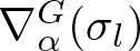 $\nabla^G_\alpha(\sigma_l)$ is a vector/vector-field. Hence,
 \begin{equation}\mathbf{d}X_t = \left[V + \dfrac{1}{2} \sum_{l = 1}^p \nabla^G_\alpha(\sigma_l)\right]dt + \dfrac{1}{2} \left(\sum_{l = 1}^pG_\alpha(\sigma_l)\right) dt + \sum_{l=1}^p \sigma_l dW^l_t,\end{equation}
 which can be considered as the SDE 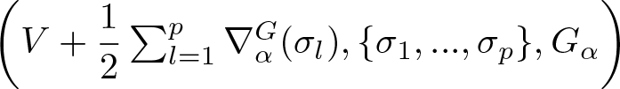 $\left(V + \dfrac{1}{2}\sum_{l = 1}^p \nabla^G_\alpha(\sigma_l),\{\sigma_1, ..., \sigma_p\}, G_\alpha \right)$.
Due to this lemma, if the manifold is equipped with a connection, then the Intrinsic SDE 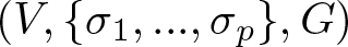 $\left(V,\{\sigma_1, ..., \sigma_p\}, G\right)$ has the Itô representation
 \begin{equation}
\left(V + \dfrac{1}{2}\sum_{l = 1}^p \nabla^G_I(\sigma_l),\{\sigma_1, ..., \sigma_p\}\right).
\end{equation}
\begin{equation}
\left(V + \dfrac{1}{2}\sum_{l = 1}^p \nabla^G_I(\sigma_l),\{\sigma_1, ..., \sigma_p\}\right).
\end{equation} Similarly, the Intrinsic SDE  $\left(V,\{\sigma_1, ..., \sigma_p\}, G\right)$ has the Stratonovich representation
 \begin{equation}
\left(V + \dfrac{1}{2}\sum_{l = 1}^p \nabla^G_S(\sigma_l),\{\sigma_1, ..., \sigma_p\}\right).
\end{equation}
\begin{equation}
\left(V + \dfrac{1}{2}\sum_{l = 1}^p \nabla^G_S(\sigma_l),\{\sigma_1, ..., \sigma_p\}\right).
\end{equation}Corollary 4.3. The Intrinsic SDE
 \begin{equation*}\left(V,\{\sigma_1, ..., \sigma_p\}, G\right)\end{equation*}
has an equivalent Belopolskya–Daletskii form that is given by
 \begin{equation}
dX_t = \exp_{X_t}\left(V(X_t)dt + \dfrac{1}{2}\sum_{l = 1}^p \nabla^G_I(\sigma_l) (X_t) dt + \sum_{l = 1}^p\sigma_l(X_t)dW^l_t\right).
\end{equation}
\begin{equation}
dX_t = \exp_{X_t}\left(V(X_t)dt + \dfrac{1}{2}\sum_{l = 1}^p \nabla^G_I(\sigma_l) (X_t) dt + \sum_{l = 1}^p\sigma_l(X_t)dW^l_t\right).
\end{equation}This statement allows us to take advantage of the underlying exponential map for numerical computations, e.g., a simple numerical method can be given by,
 \begin{equation}
X_{t+\delta t} = \exp_{X_t}(Y_{t+\Delta t} - Y_t),
\end{equation}
\begin{equation}
X_{t+\delta t} = \exp_{X_t}(Y_{t+\Delta t} - Y_t),
\end{equation} where  $Y_{t+\Delta t} - Y_t = \left[V(X_t) + \dfrac{1}{2}\sum_{l = 1}^p \nabla^G_I(\sigma_l(X_t))\right]\Delta t + \sum_{l=1}^p\sigma_l(X_t) \Delta W^l_t.$
Instead of converting Intrinsic SDE into Belopolskya–Daletskii form, one may also choose to convert the Intrinsic SDE into a Stratonovich SDE and use numerical methods for Stratonovich SDEs on manifolds from [Reference Castell and Gaines8, Reference Malham and Wiese22]. Alternatively, the option of numerical computations in a local chart is always available.
4.2. Extended Itô formula on manifolds
Let us consider the probability space  $(\Omega,\mathcal{F},\mathtt{P})$ with filtration
  $\{\mathcal{F}_t\}$. Let
  $F:\Omega\times \mathbb{R}\times \mathbb{R}^n\to \mathbb{R}^m$ be such that for the constant
  $x$,
$x$,  $F(t,x)$ is a random process given by
 \begin{equation*}d F^i(t,x) = \sum_{l=1}^p \Phi^i_l(t,x) d Y^l_t,\end{equation*}
 with  $Y_t\in\mathbb{R}^p$ as a driving semimartingale and
  $\Phi(t,x)$ as an adapted process for all
  $x\in\mathbb{R}^n$ with infinite smoothness in
  $x$. If
  $X_t$ is a semimartingale on
  $\mathbb{R}^n$, then
 \begin{equation*}d F^i(t,X_t) =D_2F^i(t,X_t) dX_t + \sum_{l=1}^p \Phi^i_l(t,X_t) dY^l_t \end{equation*}
 \begin{equation}
+ \dfrac{1}{2}\sum_{j=1}^n\sum_{k=1}^n\dfrac{\partial^2}{\partial x^j \partial x^k}F^i(t,X_t)d[X_t^j,X_t^k] + \sum_{j=1}^nd\left[\dfrac{\partial}{\partial x^j}F^i(t,X_t),X^j_t\right].
\end{equation}
\begin{equation}
+ \dfrac{1}{2}\sum_{j=1}^n\sum_{k=1}^n\dfrac{\partial^2}{\partial x^j \partial x^k}F^i(t,X_t)d[X_t^j,X_t^k] + \sum_{j=1}^nd\left[\dfrac{\partial}{\partial x^j}F^i(t,X_t),X^j_t\right].
\end{equation}This formula is known as the extended Itô formula. It is also known by other names such as the generalized Itô formula or the Itô–Wentzell formula (also spelled Itô–Ventzel), credited to A D Ventzel for its discovery in [4]. It is usually derived by proving the convergences of infinitesimal increments to the corresponding Itô integrals. The reader can refer to [Reference Kunita19, Reference Kunita20] for more details on the derivation of the formula. The generalized Itô formula is used in the area of Partial Differential Equations [Reference Bethencourt de Leon, Holm, Luesink and Takao7, Reference Constantin and Iyer11]. Some of the variants of this formula can be found in [Reference Bethencourt de Leon, Holm, Luesink and Takao7, Reference Catuogno and Stelmastchuk10] for differential k-forms, [Reference Castrequini, Catuogno and Hernandez9, Reference Keller and Zhang17, Reference Krylov18] for rough paths, and distribution-valued functions in [Reference Krylov18].
On manifolds, the generalized Itô formula is usually considered in terms of the Stratonovich representation and can be easily found, e.g., in [Reference Kunita19]. In this section, we give an equivalent formula for the Intrinsic SDEs on manifolds from the viewpoint of the diffusion generators. For this, we consider the conversion formula from the previous section to convert the Intrinsic SDE with diffusion generator into Stratonovich SDE and vice-versa.
To begin with, let us consider the Stratonovich representation on Euclidean spaces. If
 \begin{equation}
\delta F^i(t,x) = \sum_{l=1}^p \nu^i_l(t,x)\delta Y^l_t
\end{equation}
\begin{equation}
\delta F^i(t,x) = \sum_{l=1}^p \nu^i_l(t,x)\delta Y^l_t
\end{equation} such that for every  $x$,
$x$,  $\nu^i_l(l,x)$ are adapted processes that are
  $\mathcal{C}^2$ in
  $x$, and
  $F^i(t,x)$ is
  $\mathcal{C}^3$ smooth in
  $x$, then as per the generalized Itô formula,
 \begin{equation}
\delta F^i(t,X_t) = \sum_{l=1}^p \nu^i_l(t,X_t)\delta Y^l_t + D_2F^i(t,X_t)\delta X_t.
\end{equation}
\begin{equation}
\delta F^i(t,X_t) = \sum_{l=1}^p \nu^i_l(t,X_t)\delta Y^l_t + D_2F^i(t,X_t)\delta X_t.
\end{equation} On manifolds, if  $X_t\in M$ and
  $F_t:M\to N$ is a stochastically evolving smooth function such that it satisfies
 \begin{equation}
\delta F_t(x) = \sum_{l=1}^p \nu_l(t,x)\delta Y^l_t,
\end{equation}
\begin{equation}
\delta F_t(x) = \sum_{l=1}^p \nu_l(t,x)\delta Y^l_t,
\end{equation} with  $\nu_l(t,x)\in TN$ as adapted processes that are
  $\mathcal{C}^2$ smooth in
  $x$,
$x$,  $\tau_N(\nu_l(t,x)) = F_t(x)$, and
  $Y_t$ as a semimartingale on
  $\mathbb{R}^p$; then the generalized Itô formula for
  $F_t(X_t)\in N$ is given by
 \begin{equation}
\delta F_t(X_t) = \sum_{l=1}^p \nu_l(t,X_t)\delta Y^l_t + TF_t \delta X_t.
\end{equation}
\begin{equation}
\delta F_t(X_t) = \sum_{l=1}^p \nu_l(t,X_t)\delta Y^l_t + TF_t \delta X_t.
\end{equation}The generalized Itô formula on manifolds in the Stratonovich representation, given by the equation (4.13), is well known and can easily be verified by considering the local coordinates. The reader can refer to [Reference Kunita19] for variants of the generalized Itô formula on manifolds in the Stratonovich sense.
As a direct extension, in the spirit of the Schwartz–Meyer interpretation of SDEs on manifolds, the generalized Itô formula can also be expressed in terms of Stratonovich morphism. Suppose that we have a family of Stratonovich morphisms  $S_x$, between manifold
  $P$ and manifold
  $N$, which is parametrized by points
  $x\in M$, i.e.,
  $S_x = S(\cdot,\cdot;x)\in\Gamma(L(TP,TN))$ is a field of Stratonovich operators for every
  $x\in M$. This means that for a semimartingale
  $Y_t\in P$ and for a fixed point
  $x\in M$, there exits a semimartingale
  $Z^x_t = F_t(x)$ such that
 \begin{equation}
\delta Z^x_t = S_x(Y_t,Z^x_t)\delta Y_t.
\end{equation}
\begin{equation}
\delta Z^x_t = S_x(Y_t,Z^x_t)\delta Y_t.
\end{equation} We say that the above equation has a solution, given by  $H_t\in\mathcal{C}^3(M,N)$, if
  $H_t$ is a stochastically varying smooth function such that, for each point
  $x\in M$, it satisfies
  $\delta H_t(x) = S_x(Y_t,H_t(x))\delta Y_t$ in the strong sense in all the charts.
If we assume that  $F_t\in\mathcal{C}^3(M,N)$ is a solution for the SDE (4.14), then in some local coordinates on the manifold
  $P$ and manifold
  $N$, we get
 \begin{equation*}\delta F^i_t(x) = S_x{}^i_j(Y_t,F_t(x))\delta Y^j_t.\end{equation*}
 Moreover,  $F_t(x)$ is an adapted process for every
  $x\in M$. This means that if
 \begin{equation*}\nu^i_j(t,x) = S_x{}^i_j(Y_t,F_t(x)),\end{equation*}
 then by the usual Itô’s formula,  $\nu^i_j(t,x)$ are also adapted processes that are
  $\mathcal{C}^3$ smooth in
  $x$ (necessary smoothness of
  $S$ with respect to
  $x$ is assumed). This allows us to use the local Stratonovich version of the generalized Itô formula, which is given by the equation (4.11). Accordingly, we find that if
  $X_t$ is a semimartingale on
  $M$ then
 \begin{equation}
\delta F^i_t(X_t) = S^i_j(Y_t,F_t(X_t);X_t)\delta Y^j_t + \partial_j F^i_t(X_t)\delta X^j_t.
\end{equation}
\begin{equation}
\delta F^i_t(X_t) = S^i_j(Y_t,F_t(X_t);X_t)\delta Y^j_t + \partial_j F^i_t(X_t)\delta X^j_t.
\end{equation}Since this is true for all the charts, we can say that if the SDE
 \begin{equation}
\delta F(t,x) = S_x(Y_t,F(t,x))\delta Y_t
\end{equation}
\begin{equation}
\delta F(t,x) = S_x(Y_t,F(t,x))\delta Y_t
\end{equation}has a solution, then
 \begin{equation}
\delta F(t,X_t) = S_{X_t}(Y_t,F(t,X_t))\delta Y_t + T_2F(t,X_t)\delta X_t.
\end{equation}
\begin{equation}
\delta F(t,X_t) = S_{X_t}(Y_t,F(t,X_t))\delta Y_t + T_2F(t,X_t)\delta X_t.
\end{equation} Equation (4.17) can also be interpreted as a stochastic process  $Z_t = F(t,X_t)$ obtained by the driver
  $(t,Y_t,X_t)\in \mathbb{R}\times P\times M$ and the Stratonovich morphism
  $O((t,y,x),z):\mathbb{R}\times T_yP\times T_xM\to T_zN$ such that in matrix representation
 \begin{equation}
O((t,y,x),z) = \begin{bmatrix}
0 & S_x(y,z) & T_2F(t,x)
\end{bmatrix}.
\end{equation}
\begin{equation}
O((t,y,x),z) = \begin{bmatrix}
0 & S_x(y,z) & T_2F(t,x)
\end{bmatrix}.
\end{equation} In other words, if  $\delta F(t,x) = S_x(Y_t,F(t,x))\delta Y_t$ for all
  $x\in M$, then the process
  $Z_t = F(t,X_t)$ can be represented by the Stratonovich SDE
 \begin{equation}
\delta Z_t = O((t,Y_t,X_t),Z_t)\delta(t,Y_t,X_t),
\end{equation}
\begin{equation}
\delta Z_t = O((t,Y_t,X_t),Z_t)\delta(t,Y_t,X_t),
\end{equation} where the field of Stratonovich morphism  $O$ is given by equation (4.18).
In this section, we are interested in considering the extended Itô formula for the SDEs given in terms of Schwartz morphisms instead of Stratonovich morphisms. From theorem 1.2, we know that for every Stratonovich morphism there exists a Schwartz morphism. However, the converse is not true. Therefore, obtaining Itô–Wentzell formula is a challenging task when the underlying stochastic process  $F(t,x)\in N$ is given by a Schwartz SDE with an arbitrary Schwartz morphism. As the framework of the diffusion generators allows for seamless transition between the Schwartz SDE representation and the Stratonovich SDE representation, we can derive Itô–Wentzell formula in the framework of the diffusion generators. This derivation is the main contribution of this section.
Before stating the proposition for the generalized Itô’s formula, we introduce some notations that will be used throughout the remainder of this section.
(i) Manifolds
$M$ and
$N$ are equipped with the diffusion generators
${}^M G$ and
${}^N G$, respectively.(ii) We will consider
$\alpha,\beta_l\in\mathfrak{X}(M)$ for
$l\in \{1,2, ..., p\}$. We will use
$a(t)$ and
$B_l(t)$ as a short-hand notation for
$\alpha(X_t)$ and
$\beta_l(X_t)$, respectively, with
$X_t\in M$ as a semi-martingale.(iii) The Stratonovich diffusion generator on the product manifold
$M\times N$ is given by
$G_S$. The Stratonovich diffusion generator on the manifold
$N$ is given as
$G^N_S$ and as
$G^M_S$ on manifold
$M$. Moreover,
$\nabla^{{}^{N}G}_S = {}^NG - G^N_S$ and
$\nabla^{{}^MG}_S = {}^MG - G^M_S$.(iv) If
$V\in\mathfrak{X}(M\times N)$ splits as
$V = (V_1,V_2)$, i.e.,
$V_1(x,y)\in T_xM$ and
$V_2(x,y)\in T_yN$ for all
$(x,y)\in M\times N$; then the
$2^{nd}$ part of the Stratonovich diffusion generator
$G_S$, denoted by
${}^{N}G_S$, is locally (in chart
$(U,\chi)$ on
$N$) given as
(4.20)\begin{equation}
^{N}G_S(V_2)|_U = dV_2^i\cdot V \partial_i + V_2^iV_2^j\partial^2_{ij}.
\end{equation}


Proposition 4.4. Suppose  $F:\mathbb{R}\times M\to N$ is a solution of the equation
 \begin{equation}
\mathbf{d}(F(t,x)) = \left[V(x,F(t,x)) + \dfrac{1}{2} \sum_{l = 1}^p {}^N G(\sigma_l (x,F(t,x)))\right]dt + \sum_{l=1}^p \sigma_l (x,F(t,x)) dW^l_t,
\end{equation}
\begin{equation}
\mathbf{d}(F(t,x)) = \left[V(x,F(t,x)) + \dfrac{1}{2} \sum_{l = 1}^p {}^N G(\sigma_l (x,F(t,x)))\right]dt + \sum_{l=1}^p \sigma_l (x,F(t,x)) dW^l_t,
\end{equation} where  $V(x,\cdot), \sigma_1(x,\cdot), ..., \sigma_l(x,\cdot)\in \mathfrak{X}(N)$ for all
  $x\in M$ such that they are smooth in
  $x$. Let
  $X_t$ be a semimartingale on
  $M$ such that
 \begin{equation*}\mathbf{d}X_t = \left[a(t) + \dfrac{1}{2} \sum_{l = 1}^p {}^MG(B_l(t))\right]dt + \sum_{l=1}^p B_l(t) dW^l_t.\end{equation*}
Then,
 \begin{equation}
\begin{aligned}
&\mathbf{d}(F(t,X_t))= \left[ V(X_t,F(t,X_t)) + T_2F(t,X_t)a(t)\right] dt\\
&+\dfrac{1}{2}\sum_{l=1}^p \left[\nabla^{{}^N G}_S(\sigma_l (X_t,F(t,X_t))) + {}^NG_S\left(\sigma_l(X_t,F(t,X_t)) + T_2F(t,X_t)B_l(t)\right)\right] dt\\
&+ \dfrac{1}{2} \sum_{l = 1}^pT_2F(t,X_t) \nabla^{{}^M G}_S(B_l(t)) dt+\sum_{l=1}^p \left[ \sigma_l(X_t,F(t,X_t)) + T_2F(t,X_t)B_l(t)\right] dW^l_t.
\end{aligned}
\end{equation}
\begin{equation}
\begin{aligned}
&\mathbf{d}(F(t,X_t))= \left[ V(X_t,F(t,X_t)) + T_2F(t,X_t)a(t)\right] dt\\
&+\dfrac{1}{2}\sum_{l=1}^p \left[\nabla^{{}^N G}_S(\sigma_l (X_t,F(t,X_t))) + {}^NG_S\left(\sigma_l(X_t,F(t,X_t)) + T_2F(t,X_t)B_l(t)\right)\right] dt\\
&+ \dfrac{1}{2} \sum_{l = 1}^pT_2F(t,X_t) \nabla^{{}^M G}_S(B_l(t)) dt+\sum_{l=1}^p \left[ \sigma_l(X_t,F(t,X_t)) + T_2F(t,X_t)B_l(t)\right] dW^l_t.
\end{aligned}
\end{equation}Proof. In Stratonovich representation,
 \begin{equation*}\delta X_t = \left[a(t) + \dfrac{1}{2} \sum_{l = 1}^p \nabla^{{}^M G}_S(B_l(t))\right]dt + \sum_{l=1}^p B_l(t)\circ dW^l_t,\end{equation*}
and
 \begin{equation*}\delta (F(t,x)) = \left[V(x,F(t,x)) + \dfrac{1}{2} \sum_{l = 1}^p \nabla^{{}^N G}_S(\sigma_l (x,F(t,x)))\right]dt+ \sum_{l=1}^p \sigma_l (x,F(t,x)) \delta W^l_t.\end{equation*}
 As we are given that the stochastically varying function  $F_t$ is smooth enough and it satisfies the given SDE in the strong sense, the Itô–Wentzell formula given by equation 4.17 gives,
 \begin{equation*}\delta F(t,X_t) = \left[V(X_t,F(t,x)) + \dfrac{1}{2} \sum_{l = 1}^p \nabla^{{}^N G}_S(\sigma_l (X_t,F(t,x)))\right]_{x = X_t} dt\end{equation*}
 \begin{equation*}+ \sum_{l=1}^p \sigma_l (X_t,F(t,x))\big\vert_{x = X_t} \circ dW^l_t + T_2F(t,X_t) \delta X_t\end{equation*}
 \begin{equation*}= \left[ V(X_t,F(t,X_t)) + T_2F(t,X_t)a(t) + \dfrac{1}{2} \sum_{l = 1}^p \nabla^{{}^N G}_S(\sigma_l (X_t,F(t,X_t)))\right] dt\end{equation*}
 \begin{equation*}+ \dfrac{1}{2} \sum_{l = 1}^pT_2F(t,X_t) \nabla^{{}^M G}_S(B_l(t)) dt+\sum_{l=1}^p \left[ \sigma_l (X_t,F(t,X_t)) + T_2F(t,X_t)B_l(t)\right] \circ dW^l_t.\end{equation*}
 Considering  $Z_t = F(t,X_t)$, we get
 \begin{equation*}\delta Z_t = \left[ V(X_t,Z_t) + T_2F(t,X_t)a(t) + \dfrac{1}{2} \sum_{l = 1}^p \nabla^{{}^N G}_S(\sigma_l (X_t,Z_t))\right] dt\end{equation*}
 \begin{equation*}+ \dfrac{1}{2} \sum_{l = 1}^pT_2F(t,X_t) \nabla^{{}^M G}_S(B_l(t)) dt+\sum_{l=1}^p \left[ \sigma_l (X_t,Z_t) + T_2F(t,X_t)B_l(t)\right] \circ dW^l_t.\end{equation*}
 Using  $G_S$, the Stratonovich diffusion generator on
  $M\times N$, we can directly obtain the Intrinsic Schwartz SDE representation for
  $(X_t,Z_t)\in M\times N$ from its Stratonovich representation. However, it can be verified locally that the Schwartz SDE for
  $Z_t\in N$ can be obtained from its Stratonovich representation using
  ${}^NG_S$ from equation (4.20), and it is given as
 \begin{equation*}\mathbf{d} Z_t = \left[ V(X_t,Z_t) + T_2F(t,X_t)a(t) + \dfrac{1}{2} \sum_{l = 1}^p \nabla^{{}^N G}_S(\sigma_l (X_t,Z_t))\right] dt\end{equation*}
 \begin{equation*}+ \dfrac{1}{2} \sum_{l = 1}^p\left[T_2F(t,X_t) \nabla^{{}^M G}_S(B_l(t)) + {}^NG_S\left[ \sigma_l (X_t,Z_t) + T_2F(t,X_t)B_l(t)\right]\right]dt\end{equation*}
 \begin{equation*}+\sum_{l=1}^p \left[ \sigma_l (X_t,Z_t) + T_2F(t,X_t)B_l(t)\right] dW^l_t,\end{equation*}
 where  $Z_t = F(t,X_t)$.
Equation (4.22) is the extended Itô formula on manifolds when the semimartingale  $X_t\in M$ is in the Intrinsic representation with the given diffusion generator. If
  $X_t\in M$ is given as a Stratonovich SDE, then the extended Itô formula on manifolds is given by equation (4.24) in the following statement.
Corollary. Let  $F:\mathbb{R}\times M\to N$ be the solution of the SDE
 \begin{equation}
\mathbf{d}(F(t,x)) = \left[V(x,F(t,x)) + \dfrac{1}{2} \sum_{l = 1}^p {}^N G(\sigma_l (x,F(t,x)))\right]dt + \sum_{l=1}^p \sigma_l (x,F(t,x)) dW^l_t;
\end{equation}
\begin{equation}
\mathbf{d}(F(t,x)) = \left[V(x,F(t,x)) + \dfrac{1}{2} \sum_{l = 1}^p {}^N G(\sigma_l (x,F(t,x)))\right]dt + \sum_{l=1}^p \sigma_l (x,F(t,x)) dW^l_t;
\end{equation} where  $V(x,\cdot), \sigma_1(x,\cdot), ..., \sigma_l(x,\cdot)\in \mathfrak{X}(N)$ for all
  $x\in M$. Let
  $X_t$ be a semimartingale on
  $M$, with Stratonovich representation as
 \begin{equation*}\delta X_t = a(t)dt + \sum_{l=1}^p B_l(t)\circ dW^l_t,\end{equation*}
 where  $a(t)$ and
  $B_l(t)$ is a short-hand notation for
  $\alpha(X_t)$ and
  $\beta_l(X_t)$, respectively, for some
  $\alpha,\beta_l\in\mathfrak{X}(M).$ Then,
 \begin{equation}
\begin{aligned}
&\mathbf{d}(F(t,X_t))= \left[ V(X_t,F(t,X_t)) + T_2F(t,X_t)a(t)\right] dt\\
&+\dfrac{1}{2}\sum_{l=1}^p \left[\nabla^{{}^N G}_S(\sigma_l (X_t,F(t,X_t))) + {}^NG_S\left(\sigma_l(X_t,F(t,X_t)) + T_2F(t,X_t)B_l(t)\right)\right] dt\\
&+\sum_{l=1}^p \left[ \sigma_l(X_t,F(t,X_t)) + T_2F(t,X_t)B_l(t)\right] dW^l_t.
\end{aligned}
\end{equation}
\begin{equation}
\begin{aligned}
&\mathbf{d}(F(t,X_t))= \left[ V(X_t,F(t,X_t)) + T_2F(t,X_t)a(t)\right] dt\\
&+\dfrac{1}{2}\sum_{l=1}^p \left[\nabla^{{}^N G}_S(\sigma_l (X_t,F(t,X_t))) + {}^NG_S\left(\sigma_l(X_t,F(t,X_t)) + T_2F(t,X_t)B_l(t)\right)\right] dt\\
&+\sum_{l=1}^p \left[ \sigma_l(X_t,F(t,X_t)) + T_2F(t,X_t)B_l(t)\right] dW^l_t.
\end{aligned}
\end{equation}Proof. To convert the Stratonovich SDE for  $X_t\in M$ into its Schwartz representation, we consider the Stratonovich diffusion generator on
  $M$, denoted by
  $G^M_S$. Therefore, in proposition 4.4, we consider the given diffusion generator
  ${}^MG$ to be the same as
  $G^M_S$. Then
  $\nabla^{{}^MG}_S = {}^MG - G^M_S = 0$.
Example. Using the generalized Itô formula, we can answer the motivational question introduced at the end of Section 1.2. To recall, we consider  $L\in \mathfrak{F}(TM)$ as a regular Lagrangian with associated energy
  $E\in \mathfrak{F}(TM)$.
  $X_t\in M$ satisfies
 \begin{equation}
\delta X_t = Z_t dt + \sum_{l = 1}^p T\tau_M\sigma_l(Z_t) \delta W_t^l,
\end{equation}
\begin{equation}
\delta X_t = Z_t dt + \sum_{l = 1}^p T\tau_M\sigma_l(Z_t) \delta W_t^l,
\end{equation} where  $\sigma_l\in Ker(dE)$, and
  $Z_t\in TM$ such that
  $X_t = \tau_M(Z_t)$ and it satisfies
 \begin{equation}
\delta Z_t = \omega^\sharp_L dE(Z_t) dt + \sum_{l = 1}^p\sigma_l(Z_t) \delta W_t^l.
\end{equation}
\begin{equation}
\delta Z_t = \omega^\sharp_L dE(Z_t) dt + \sum_{l = 1}^p\sigma_l(Z_t) \delta W_t^l.
\end{equation} We are interested in finding an SDE for a stochastically varying vector field  $F_t\in \mathfrak{X}(M)$ that satisfies
  $Z_t = F_t(X_t)$.
Using the generalized Itô formula, we immediately observe that if there exists  $F_t:M\to TM$ such that
  $F_t(X_t) = Z_t$, then for every
  $x\in M$,
 \begin{equation}
\delta F_t(x) = (\omega^\sharp_L dE(F_t(x)) - TF_t F_t(x)) dt + \sum_{l = 1}^p \left[\sigma_l(F_t(x)) - TF_tT\tau_M\sigma_l(F_t(x)) \right]\delta W_t^l,
\end{equation}
\begin{equation}
\delta F_t(x) = (\omega^\sharp_L dE(F_t(x)) - TF_t F_t(x)) dt + \sum_{l = 1}^p \left[\sigma_l(F_t(x)) - TF_tT\tau_M\sigma_l(F_t(x)) \right]\delta W_t^l,
\end{equation} Notice that the horizontal part of the drift and the noise vector fields in the above equation is zero, which implies that the stochastic curve  $F_t(x)\in TM$ is constrained to be on the tangent space
  $T_xM$, making the map
  $F_t:M\to TM$ a vector field. Component-wise, the drift vector can also be given as
 \begin{equation*}(\omega^\sharp_L dE(F_t(x)) - TF_t F_t(x))^i = \left(0,\left[\nabla^{G_L}_S(F_t(x))\right]^i\right),\end{equation*}
 where  $G_L$ is the Lagrangian diffusion generator, and
  $0$ represents the horizontal part. Since
  $Z_t = F_t(X_t)$ is energy-preserving, the solution of (4.27), if it were to exist, is enough to describe the energy-preserving motion of the point
  $X_t\in M$ given by equation (4.25).
5. Concluding remarks
We have shown that intrinsic SDEs on manifolds can be described using diffusion generators that are constructed using the flow of ordinary differential equations. We have demonstrated that by considering diffusion generators obtained using first-order differential equations, we end up with the Schwartz representation of a Stratonovich SDE. We have also demonstrated that it is possible to obtain diffusion generator using a second-order differential equation. We have demonstrated that if this second-order differential equation is the geodesic equation, then the corresponding diffusion generator gives us the Schwartz representation of an Itô SDE. Another example of the diffusion generator obtained using the second-order differential equation is that of the Lagrangian dynamics with a regular Lagrangian.
In Section 4, we derived a formula to convert an Intrinsic SDE with a diffusion generator into an Intrinsic SDE obtained using a different diffusion generator. Using this conversion formula, we also derived the extended/generalized Itô formula on the manifolds. As an application of the extended Itô formula and an attempt to link the Lagrangian diffusion generator with the generalized Itô formula, we also present a point-wise SDE for the stochastically varying vector field such that the flow of a stochastic point along this vector field preserves the energy of the Lagrangian system.
Overall, we find that the diffusion generator approach makes the coordinate-invariant analysis of SDEs on manifolds easier.

 Open access