3.1. Approximate solution of the fourth order

To the fourth order in $\epsilon$ , we obtain the sequence of equations given by

(3.7) \begin{align} & \Phi _{4\xi \xi }+\Phi _{4\eta \eta }=0, \quad -\mu \leqslant \eta \lt 0,\\& \Phi _{4\eta }+C_{0}E_{4\xi }=-E_{1}\Phi _{3\eta \eta }-E_{2}\Phi _{2\eta \eta }-E_{3}\Phi _{1\eta \eta }-\frac {1}{2}E_{1}^{2}\Phi _{2\eta \eta \eta }-E_{1}E_{2}\Phi _{1\eta \eta \eta } \nonumber \\& \quad -\frac {1}{6}E_{1}^{3}\Phi _{1\eta \eta \eta \eta }+(\Phi _{1\xi }+\Omega {E_{1}})E_{3\xi }+(\Phi _{2\xi }+E_{1}\Phi _{1\xi \eta }+\Omega {E_{2}}-C_{2})E_{2\xi }, \nonumber \end{align}

(3.8) \begin{align} & \quad +(\Phi _{3\xi }+E_{1}\Phi _{2\xi \eta }+E_{2}\Phi _{1\xi \eta }+\frac {1}{2}E_{1}^{2}\Phi _{1\xi \eta \eta } +\Omega {E_{3}}-C_{3})E_{1\xi }, \quad \eta =0 \end{align}

(3.9) \begin{align} & C_{0}\Phi _{4\xi }-(1-C_{0}\Omega )E_{4}+\kappa {E_{4\xi \xi }}=\frac {1}{2}\left(\Phi _{2\xi }^{2}+\Phi _{2\eta }^{2}\right)+\Phi _{1\xi }\Phi _{3\xi }+\Phi _{1\eta }\Phi _{3\eta } \nonumber \\&\quad +E_{1}(\Phi _{1\xi }\Phi _{2\xi \eta }+\Phi _{2\xi }\Phi _{1\xi \eta }+\Phi _{1\eta }\Phi _{2\eta \eta }+\Phi _{2\eta }\Phi _{1\eta \eta }) +\frac {1}{2}E_{1}^{2}\left(\Phi _{1\xi \eta }^2+\Phi _{1\xi }\Phi _{1\xi \eta \eta } \right.\nonumber \\ & \quad +\left.\Phi _{1\eta \eta }^2+\Phi _{1\eta }\Phi _{1\eta \eta \eta }\right)+E_{2}(\Phi _{1\xi }\Phi _{1\xi \eta }+\Phi _{1\eta }\Phi _{1\eta \eta })+\frac {1}{2}\Omega ^2\left(E_2^2+2{E_1}{E_3}\right) \nonumber \\ & \quad +\Omega \left(E_1\Phi _{3\xi } +E_2\Phi _{2\xi }+E_3\Phi _{1\xi }+E_1^2\Phi _{2\xi \eta }+2E_1E_2\Phi _{1\xi \eta }+\frac {1}{2}E_1^3\Phi _{1\xi \eta \eta }\right) \nonumber \\ & \quad -C_0\left(E_1\Phi _{3\xi \eta }+E_2\Phi _{2\xi \eta }+E_3\Phi _{1\xi \eta } +\frac {1}{2}E_1^2\Phi _{2\xi \eta \eta }+E_1E_2\Phi _{1\xi \eta \eta }+\frac {1}{6}E_1^3\Phi _{1\xi \eta \eta \eta }\right) \nonumber \\ & \quad -C_3\left(\Phi _{1\xi }+\Omega {E_1}\right)-C_2\left(\Phi _{2\xi }+\Omega {E_2}+E_1\Phi _{1\xi \eta }\right)+\frac {3}{2}\kappa {E_{1\xi }^{2}}E_{2\xi \xi } \nonumber \\ & \quad +3\kappa {E_{1\xi }}E_{2\xi }E_{1\xi \xi } -\frac {1}{2}K_4=0, \quad \eta =0, \end{align}

(3.10) \begin{align} & \Phi _{4\eta }=0, \quad \eta =-\mu . \end{align}

Classically, we seek the solutions for the fourth-order potential and elevation amplitude in the form

(3.11) \begin{align} & \Phi _{4}(\xi ,\eta )=A_{44}\frac {\cosh [4(\eta +\mu )]}{\cosh (4\mu )}\sin (4\xi )+A_{42}\frac {\cosh [2(\eta +\mu )]}{\cosh (2\mu )}\sin (2\xi ), \end{align}

(3.12) \begin{align} &\qquad\qquad\qquad\qquad E_{4}(\xi )=a_{44}\cos (4\xi )+a_{42}\cos (2\xi ). \end{align}

Then by inserting (3.11)–(3.12) into the boundary conditions (3.8)–(3.9) and using the first-, second- and third-order solutions, after tedious algebra we obtain

(3.13) \begin{align} &A_{44}=\frac {3\epsilon }{8\left [(5+\sigma ^2)-15\overline \kappa (1+\sigma ^2)\right ]}\frac {(1+6\sigma ^2+\sigma ^4)}{\sigma ^3(1+3\sigma ^2)}\left [(1+3\sigma ^2)\overline {\Omega } +2(1-3\sigma ^2-2\sigma ^4) \right.\nonumber \\ & \quad +\left. 15\overline \kappa \sigma ^2(1+3\sigma ^2)\right ]A_{33}+\frac {C_{0}\epsilon }{8\left [(5+\sigma ^2)-15\overline \kappa (1+\sigma ^2)\right ]}\frac {(1+6\sigma ^2+\sigma ^4)}{\sigma ^4}\nonumber \\ & \quad\times\left [\overline {\Omega }^2 +\left \{2+15\overline \kappa \sigma ^2\right \}\overline {\Omega } +(1-\sigma ^2)+15\overline \kappa \sigma ^2\right ]a_{33} \nonumber \\ & \quad +\frac {C_0\epsilon ^4}{768(1-3\overline \kappa )^2\left [(5+\sigma ^2)-15\overline \kappa (1+\sigma ^2)\right ]}\frac {(1+6\sigma ^2+\sigma ^4)}{\sigma ^{10}} \nonumber \\ & \quad \times \left [3\overline {\Omega }^6+\!\left \{3(9+4\sigma ^2)+45\overline \kappa \sigma ^2\right \}\overline {\Omega }^5\!+\!\left \{12(9+3\sigma ^2+\sigma ^4)+18\overline \kappa \sigma ^2(21+11\sigma ^2)\right \}\overline {\Omega }^4 \right.\nonumber \\ & \quad +\left \{3(81-14\sigma ^2+21\sigma ^4) +9\overline \kappa \sigma ^2(149+68\sigma ^2+19\sigma ^4)+270{\overline {\kappa }}^2\sigma ^4(1+\sigma ^2)\right \}\overline {\Omega }^3 \nonumber \\ & \quad +\left \{12(27-29\sigma ^2+21\sigma ^4-4\sigma ^6)+18\overline \kappa \sigma ^2(139+18\sigma ^2+41\sigma ^4) \right.\nonumber \\ & \quad +\left. 27{\overline {\kappa }}^2\sigma ^4(51-34\sigma ^2+11\sigma ^4)\right \}\overline {\Omega }^2+\left \{3(81-192\sigma ^2+169\sigma ^4-82\sigma ^6) +9\overline \kappa \sigma ^2\right.\nonumber \\ & \quad \times\left. (273-110\sigma ^2+253\sigma ^4-12\sigma ^6) +54{\overline {\kappa }}^2\sigma ^4(47-84\sigma ^2+15\sigma ^4)-3240{\overline {\kappa }}^3\sigma ^8\right \}\overline {\Omega } \nonumber \\ & \quad +(81-342\sigma ^2+432\sigma ^4-302\sigma ^6+131\sigma ^8) +6\overline \kappa \sigma ^2(171-177\sigma ^2+359\sigma ^4-283\sigma ^6) \nonumber \\ & \quad +\left. 144{\overline {\kappa }}^2\sigma ^4(12-38\sigma ^2+43\sigma ^4)-5940{\overline {\kappa }}^3\sigma ^8\right ] , \end{align}

(3.14) \begin{align} & A_{42}=\frac {3\epsilon }{4(1-3\overline \kappa )}\frac {(1+\sigma ^2)}{\sigma ^3(1+3\sigma ^2)}\left [(1+3\sigma ^2)\overline {\Omega }+2(1-\sigma ^4)+3\overline \kappa \sigma ^2(1+3\sigma ^2)\right ]A_{33} \nonumber \\ & \quad +\frac {\epsilon }{4(1-3\overline \kappa )}\frac {(1+\sigma ^2)}{\sigma ^3}\left [\overline {\Omega }+2(1-\sigma ^2)+3\sigma ^2\overline \kappa \right ]A_{31}-\frac {\epsilon ^4}{8(1-3\overline \kappa )^2}\frac {(1+\sigma ^2)}{\sigma ^{6}} \nonumber \\ & \quad \times \left [\overline {\Omega }^3+\left \{(5+2\sigma ^2)+3\overline \kappa \sigma ^2\right \}\overline {\Omega }^2 +\left \{3(3+\sigma ^2) +6\overline \kappa \sigma ^2(2+\sigma ^2)\right \}\overline {\Omega } \right.\nonumber \\ & \quad +\left.(6-\sigma ^2-\sigma ^4)+3\overline \kappa \sigma ^2(5-\sigma ^2)\right ]C_2 +\frac {C_0\epsilon ^4}{48(1-3\overline \kappa )^2}\frac {(1+\sigma ^2)}{\sigma ^{6}}\left [18\overline {\Omega }^3 \right.\nonumber \\ & \quad +\left \{3(25+\sigma ^2)+45\overline \kappa \sigma ^2\right \}\overline {\Omega }^2 +\left \{39(3-\sigma ^2)+18\overline \kappa \sigma ^2(7-\sigma ^2) +54{\overline {\kappa }}^2\sigma ^4\right \}\overline {\Omega } \nonumber \\ & \quad +\left.(63-52\sigma ^2+13\sigma ^4) +3\overline \kappa \sigma ^2(31-23\sigma ^2) +90{\overline {\kappa }}^2\sigma ^4\right ], \end{align}

(3.15) \begin{align} & a_{44}=\frac {\tanh (4\mu )}{C_{0}}A_{44}+\frac {3\epsilon }{2C_{0}}A_{33}+\frac {\epsilon }{2\sigma }(\overline {\Omega }+1)a_{33} +\frac {\epsilon ^4}{192(1-3\overline \kappa )^2}\frac {1}{\sigma ^7}\nonumber \\ & \quad\times\left [3\overline {\Omega }^5 +12(2+\sigma ^2)\overline {\Omega }^4 +\left \{9(9+6\sigma ^2+\sigma ^4)+18\overline \kappa \sigma ^2(1+\sigma ^2)\right \}\overline {\Omega }^3\right.\nonumber \\ & \quad+\left \{12(12+7\sigma ^2+2\sigma ^4) +18\overline \kappa \sigma ^2(5+\sigma ^4)\right \}\overline {\Omega }^2 +\left \{3(45+12\sigma ^2+13\sigma ^4-2\sigma ^6)\right.\nonumber \\ & \quad+\left. 18\overline \kappa \sigma ^2(9-8\sigma ^2+3\sigma ^4) -216{\overline {\kappa }}^2\sigma ^6\right \}\overline {\Omega }+2(27-9\sigma ^2+27\sigma ^4-31\sigma ^6)\nonumber \\ & \quad +\left.12\overline \kappa \sigma ^2(9-21\sigma ^2+28\sigma ^4)-396{\overline {\kappa }}^2\sigma ^6 \right ] , \end{align}

and, furthermore,

(3.16) \begin{align} & a_{42}= \frac {\tanh (2\mu )}{C_{0}}A_{42}+\frac {3\epsilon }{2C_{0}}A_{33}+\frac {\epsilon }{2C_{0}}A_{31}-\frac {\epsilon ^2}{C_{0}}(C_{2}a_{2})+\frac {\epsilon ^4}{24(1-3\overline \kappa )}\frac {1}{\sigma ^3} \nonumber \\ & \quad \times \left [9\overline {\Omega }^2 +\left \{3(9+\sigma ^2)+18\overline \kappa \sigma ^2\right \}\overline {\Omega }+(27-19\sigma ^2)+30\overline \kappa \sigma ^2\right ], \end{align}

(3.17) \begin{align} & K_4=\frac {C_0\epsilon }{\sigma }(\overline {\Omega }+1)A_{31}+\frac {C_0^2\epsilon }{\sigma ^2}(\overline {\Omega }^2+\overline {\Omega }-\sigma ^2)a_{31}-\epsilon ^4 C_0 C_2+\frac {C_0^2\epsilon ^4}{32(1-3\overline \kappa )^2}\frac {1}{\sigma ^8} \nonumber \\ & \quad \times \left [\overline {\Omega }^6+4(2+\sigma ^2)\overline {\Omega }^5 +\left \{4(7+4\sigma ^2+\sigma ^4)+6\overline \kappa \sigma ^2(1+\sigma ^2)\right \}\overline {\Omega }^4\right.\nonumber \\ & \quad+\left \{2(27+8\sigma ^2+9\sigma ^4) +12\overline \kappa \sigma ^2(3-2\sigma ^2+\sigma ^4)\right \}\overline {\Omega }^3\nonumber \\ & \quad+\left \{12(5-2\sigma ^2+5\sigma ^4)+12\overline \kappa \sigma ^2(7-14\sigma ^2+2\sigma ^4) +9{\overline {\kappa }}^2\sigma ^4(1-10\sigma ^2+\sigma ^4)\right \}\overline {\Omega }^2\nonumber \\ & \quad +\left \{12(3-5\sigma ^2+9\sigma ^4-2\sigma ^6) +6\overline \kappa \sigma ^2(15-53\sigma ^2+27\sigma ^4-\sigma ^6)+36{\overline {\kappa }}^2\sigma ^4(1-6\sigma ^2)\right \} \nonumber \\ & \quad \times\overline {\Omega }+(9-36\sigma ^2+78\sigma ^4-40\sigma ^6+9\sigma ^8)+12\overline \kappa \sigma ^2(3-15\sigma ^2+12\sigma ^4-4\sigma ^6) \nonumber \\ & \left.\quad +36{\overline {\kappa }}^2\sigma ^4(1-9\sigma ^2+2\sigma ^4)\vphantom{\overline {\Omega }^6} \right ], \end{align}

(3.18) \begin{align} &\qquad\qquad\qquad\qquad\qquad\qquad\qquad\qquad C_3=0. \end{align}

Equations (3.13)–(3.18) constitute the main analytical results of this study and extend the third-order analysis initiated by Hsu et al. (Reference Hsu, Francius, Montalvo and Kharif2016). In the next section we shall use these relations to describe the improvements gained with the fourth-order approximation by analysing not only the surface profiles but also the internal flow velocities.

Not surprisingly, the fourth-order approximation is found to be invalid when $\kappa$ equals another critical value, $\kappa _3$ , the root of the following equation:

(3.19) \begin{align} \kappa =\frac {(5+\sigma ^2)\sigma ^2}{15(1+\overline {\Omega })+5(2+3\overline {\Omega })\sigma ^2-\sigma ^4}. \end{align}

Without vorticity, (3.19) becomes

(3.20) \begin{align} \kappa _3=\frac {(5+\sigma ^2)\sigma ^2}{15+10\sigma ^2-\sigma ^4} \end{align}

in agreement with the results of Barakat & Houston (Reference Barakat and Houston1968). This latter equation reduces in deep water ( $\sigma =1$ ) to the other well-known value $\kappa _3=1/4$ .

3.2. Critical wavenumbers

Since the pioneering works of Harrison (Reference Harrison1909) and Pierson & Fife (Reference Pierson and Fife1961), it is well known that the application of the Stokes expansion method for the periodic steady irrotational GC wave problem, either in deep water or finite depth, is not legitimate when $\kappa$ is close to the critical values $\kappa _n$ ( $n\geqslant 1)$ , which form, when they exist, an infinite discrete set of critical values. At these critical values, it is observed that there is a lack of uniqueness in the linear solution. Physically, it can be explained by a resonance mechanism due to the fact that infinitesimal waves of wavenumber $k_0$ and $nk_0$ have the same phase velocity when $\kappa =\kappa _n$ .

For irrotational GC waves on finite depth, Barakat & Houston (Reference Barakat and Houston1968) remarked that the $n$ th approximation obtained with the classical Stokes expansion method breaks down when $\kappa =\kappa _{n-1}$ , the roots of the following equations:

(3.21) \begin{align} \kappa =\frac {n\tanh \mu -\tanh (n\mu )}{n^2\tanh (n\mu )-n\tanh \mu }, \quad \quad n \geqslant 2. \end{align}

In deep water these roots have the well-known values $\kappa _{n-1}=1/n$ ( $n\geqslant 2$ ). Solutions that bifurcate from these critical values are the so-called Wilton ripples, which correspond to resonances between the fundamental and the nth harmonic. For $n=4$ , with some algebra one can show that (3.21) corresponds to (3.20).

If the dependence between the dimensionless parameters $\kappa$ and $\mu$ is not considered, graphs of $\kappa _n$ versus $\mu$ may be misleading with respect to the interpretation of the influence of the depth of the fluid layer. It should be realized that the critical numbers are the roots $\kappa _{n-1}$ of the following equations for $n\geqslant 2$ :

(3.22) \begin{align} \kappa \left [ n^2\tanh (n\kappa ^{1/2} \tilde {h})-n\tanh (\kappa ^{1/2} \tilde {h}) \right ] - \left [n\tanh (\kappa ^{1/2} \tilde {h})-\tanh (n \kappa ^{1/2} \tilde {h})\right ]=0, \end{align}

obtained from (3.21) and the relation $\mu =\kappa ^{1/2}\tilde {h}$ , where $\tilde {h}=k_c h_0$ and $k_c=\sqrt {\rho g/T}$ . Numerical calculations were performed for water ( $T=74\,\rm dynes\,cm^-{^1}$ ), by using a variant of the Newton–Raphson method to solve (3.22) for $\kappa$ . The results for the first three critical values are shown in figure 1 as a function of $\tilde {h}$ . The dotted lines represent the well-known asymptotic values of $\kappa _n$ ( $n=1,2$ and $3$ ) for irrotational GC waves in deep water. The thin solid lines are drawn to show the dependency of the dimensionless number $\kappa$ on the depth layer $\tilde {h}$ for fixed values of $\mu$ . The thin solid lines of figure 1 are drawn for $\mu =10,2$ and $1$ .

Figure 1. Variations of $\kappa _1,\kappa _2,\kappa _3$ as a function of depth for water for irrotational GC waves. In any case $\kappa _1\gt \kappa _2\gt \kappa _3$ . The dotted lines represent the corresponding deep-water values. Using a separate y-axis, the relation $\mu =\kappa ^{1/2}\tilde {h}$ is plotted for $\mu =10,2$ and $1$ (from the right to the left).

As shown in figure 1 the critical values $\kappa _n$ decrease rapidly with decreasing $\tilde {h}$ , and eventually disappear when $\tilde {h} \lt \tilde {h}_c=\sqrt {3}$ . It is noticed that these results match those of figure 2 in Barakat & Houston (Reference Barakat and Houston1968). For water $\tilde {h}_c=\sqrt {3}$ corresponds to the particular water depth 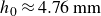$h_0\approx 4.76\,\rm mm$ . In fact, when the surface tension is large, or equivalently, the fluid depth is sufficiently small so that $\tilde {h} \lt \tilde {h}_c$ , the phase velocity is strictly a monotonic function of the wavenumber, and thus no resonances are possible. In other words, when $\tilde {h} \lt \tilde {h}_c$ the asymptotic expansion of the solution is regular to any order, as demonstrated by Nayfeh (Reference Nayfeh1970a ) who considered the limit $\mu \ll 1$ . In contrast, when $\tilde {h} \gt \tilde {h}_c=\sqrt {3}$ resonances between the fundamental and the nth harmonic are possible. Figure 1 also indicates that using the asymptotic theory with a constant value of $\mu$ , the fundamental dimensional wavenumber $k_0$ being kept fixed, the first three singularities are found at the intersections between the corresponding thin solid line and the curves in thick solid lines. It should be emphasized that for a given $\mu$ each critical value of the wavenumber corresponds indeed to a different physical depth of the fluid layer. Nonetheless, for $\tilde {h}\gt 5$ , the effects of the depth are negligible and the GC waves may be regarded as deep-water phenomena.

It is possible to generalize the approach of Barakat & Houston (Reference Barakat and Houston1968) to the case of GC waves with constant vorticity in finite depth. Namely, for steadily travelling periodic waves it is expected that the nth-order approximation obtained with the classical Stokes expansion method will break down when the wavenumber $k_0$ satisfies the following relation:

(3.23) \begin{align} C_* (k_0)= C_* (n k_0) \end{align}

or equivalently in dimensionless form, considering only forward propagating modes,

(3.24) \begin{align} -\frac {\Omega }{2} \alpha _1 + \sqrt {\left (\frac {\Omega \alpha _1}{2}\right )^2+(1 +\kappa ) \alpha _1} = -\frac {\Omega }{2} \alpha _n + \sqrt {\left (\frac {\Omega \alpha _n}{2}\right )^2+(1 +n^2\kappa ) \alpha _n} , \end{align}

where $n\alpha _n= \tanh (n \mu )$ . With elementary relations for hyperbolic functions and some algebra, it can be shown that (3.24) yields the equations (A12), (B12) and (3.19) when $n=2,3$ and $4$ (respectively), and therefore represents the extension of (3.21) in the presence of current shear. Introducing $\tilde {\Omega }=\Omega _0/\sqrt {g k_c}$ and using the relation $\Omega =\kappa ^{-1/4}\tilde {\Omega }$ , one can see that (3.24) defines a nonlinear equation for $\kappa$ for fixed values of the two intrinsic dimensionless parameters, $\tilde {h}$ and $\tilde {\Omega }$ . It should be emphasized here that in the analysis carried out by Hsu et al. (Reference Hsu, Francius, Montalvo and Kharif2016) the fully implicit definition of the critical wavenumbers was not properly recognized. More explicitly, the relation $\Omega =\kappa ^{-1/4}\tilde {\Omega }$ was not taken into account when solving for the roots of (B11) and (B12). This gives rise to ambiguous results, as for instance the doubling of the critical wavenumbers at second and third order when $\Omega \lt 0$ for a given fixed ‘physical’ dimensionless depth $\tilde {h}$ (see figure 2 in Hsu et al. (Reference Hsu, Francius, Montalvo and Kharif2016)). Though the plotted results in figure 2 of Hsu et al. (Reference Hsu, Francius, Montalvo and Kharif2016) are correct, their interpretation may be misleading.

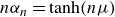
Figure 2. Variations of $\kappa _1,\kappa _2,\kappa _3$ as a function of depth for water for different values of the shear parameter: (a) $\tilde {\Omega }=\pm 0.5$ ; (b) $\tilde {\Omega }=\pm 0.9$ . In any case $\kappa _1\gt \kappa _2\gt \kappa _3$ ; dashed lines correspond to positive values of $\tilde {\Omega }$ , dash–dotted lines to negative ones and thin solid lines are drawn for $\mu =10, 2$ and $1$ (from the right to the left).

Numerical calculations were also performed for water ( $T=74$ dynes/cm) to solve (3.24) for $\kappa$ . The results for the first three critical values are shown in figure 2 as a function of $\tilde {h}$ with four different values of the shear parameter $\tilde {\Omega }$ . In any case it is seen that there is still a critical depth, $\tilde {h}_*$ , below which resonances are not possible, although it depends on the value of the vorticity. When resonances are possible, namely when $\tilde {h}\gt \tilde {h}_*$ , we always have $\kappa _1\gt \kappa _2\gt \kappa _3$ and their values are, of course, different from the irrotational case. Figure 2 shows that these critical values increase (decrease) with increasing positive (negative) vorticity. Interestingly, given that $\kappa _1$ decreases with increasing (negative) vorticity when $\tilde {h}\gt \tilde {h}_*$ , the interval $[\kappa _1,\infty [$ , over which the asymptotic theory is regular, also increases.

Actually the dependency of $\tilde {h}_*$ on the shear parameter $\tilde {\Omega }$ can be analysed with the analytical results obtained by Martin (Reference Martin2013). As far as we are concerned with the forward propagating mode, we can use his Lemma 3 to write the appropriate relationship in dimensionless form, as

(3.25) \begin{align} \tilde {h}_*^2=3+ \tilde {\Omega }\tilde {h}_* \left [ \tilde {h}_*\sqrt {\tilde {h}_*+\frac {\tilde {\Omega }^2\tilde {h}_*^2}{4}}-\frac {\tilde {\Omega }\tilde {h}_*}{2}\right ]. \end{align}

Figure 3, in which the solution of (3.25) is plotted as a function of $\tilde {\Omega }$ , shows that $\tilde {h}_*\gt \sqrt {3}$ when $\tilde {\Omega }\gt 0$ and $\tilde {h}_*\lt \sqrt {3}$ when $\tilde {\Omega }\lt 0$ . In the region below the solid curve plotted in this figure, namely when $\tilde {h}\lt \tilde {h}_*$ , resonances are not possible and thus the asymptotic theory is regular for any wavenumber. Notice that Gao et al. (Reference Gao, Milewski and Wang2021) have also described the effects of vorticity on the properties of the dispersion relation and obtained identical results for the forward propagating mode. Actually the first case in their inequalities (13) correspond to the region in figure 3 where $\tilde {h}\lt \tilde {h}_*$ , which they have named shallow-water regime. Figure 3 also reveals that for any given value of the physical depth, or equivalently $\tilde {h}$ , there exist a threshold value of $\tilde {\Omega }$ above which there are no resonances. This particular value is positive when $\tilde {h}\gt \sqrt {3}$ , but negative when $\tilde {h}\lt \sqrt {3}$ . This is further illustrated in figure 4, where the critical values $\kappa _{n-1}$ ( $n=2,3\,\mathrm{and}\,4$ ) are plotted as a function of $\tilde {\Omega }$ for two particular values of the depth.

Figure 3. Normalized critical depth $\tilde {h}_*$ as a function of $\tilde {\Omega }$ .

Figure 4. Variations of $\kappa _1,\kappa _2,\kappa _3$ for different values of $\tilde {h}$ for water as a function of the shear parameter $\tilde {\Omega }$ : (a) $\tilde {h}/\sqrt {3}=2$ ; (b) $\tilde {h}/\sqrt {3}=0.9$ . In any case $\kappa _1\gt \kappa _2\gt \kappa _3$ . The dotted lines represent the corresponding well-known values in deep water.

4.1. Fully nonlinear solutions

To compute steadily travelling periodic GC waves with constant vorticity in finite depth, we shall use a numerical method based on a conformal mapping method and Fourier series expansions of the unknowns, such as given by Guo et al. (Reference Guo, Tao and Zeng2014) and Choi (Reference Choi2009) for two-dimensional GC solitary waves and gravity waves, respectively. It is emphasized here that, though these authors established the governing equations for GC waves in finite depth with constant vorticity, the numerical computations were carried out only in the deep-water case. The formulation of the governing equations in the transformed plane (a canonical strip) is well documented by these authors, and therefore needs not to be reproduced here.

To be concise and consistent, however, we present the transformed governing equations used in our study and adopt the same notations as Ribeiro et al. (Reference Ribeiro, Milewski and Nachbin2017) except for the coordinates in the canonical domain. Namely the conformal map is defined as $\tilde {Z} ( \zeta ,\vartheta )=\tilde {X} ( \zeta ,\vartheta )+i\tilde {Y} ( \zeta ,\vartheta )$ and the surface elevation as $z=\eta (X)=Y(\zeta )$ where $X=\tilde {X}(\zeta ,0)$ and $Y=\tilde {Y}(\zeta ,0)$ . After performing similar calculations as those presented in Choi (Reference Choi2009), we can show that the free surface kinematic and dynamic boundary conditions can be combined into a single pseudodifferential equation for the free surface elevation $Y(\zeta )$ ,

(4.1) \begin{align} -\frac {\tilde {c}^2}{2} -\frac {\tilde {c}^2}{2 J} + Y + \gamma ^2 \frac { \left (\mathcal{C}\left [ \left (Y+b\right )Y_\zeta \right ]\right ) - \left (\left (Y+b\right )Y_\zeta \right )^2}{2 J} - \gamma \tilde {c} b & \nonumber \\ +\frac {\left (\tilde {c}+\gamma \mathcal{C}\left [ \left (Y+b\right )Y_\zeta \right ] \right ) \left (\tilde {c} +\gamma \left (Y+b\right ) \left ( 1-\mathcal{C}\left [Y_\zeta \right ]\right ) \right )}{J} + \tilde {\kappa } \frac {X_\zeta Y_{\zeta \zeta }-Y_\zeta X_{\zeta \zeta }}{J^{3/2}} & = \tilde {B}, \end{align}

where $J=\tilde {X}_\zeta ^2+\tilde {Y}_\zeta ^2$ is Jacobian of the conformal map evaluated at the free surface. According to our choice of scaling (see § 2), we have $\tilde {c}=C/\sqrt {\mu }$ , $\tilde {\kappa }=\kappa /\mu ^2$ , $\gamma =-\sqrt {\mu }\Omega$ , and $\tilde {B}$ is the Bernoulli constant. As explained in Ribeiro et al. (Reference Ribeiro, Milewski and Nachbin2017), $b$ is a free parameter that determines the choice of the reference frame, or equivalently the depth at which the Eulerian mean horizontal velocity is zero in the limit of small amplitude waves. Since the governing equations have the property of Galilean invariance, the parameter $b$ affects neither the shape of the wave nor the streamlines in the frame of reference travelling with the wave. For the comparison with the analytical results derived in § 3 we shall take $b=0$ . Equation (4.1) contains three additional unknowns, the phase velocity $\tilde {c}$ , the Bernoulli constant $\tilde {B}$ and the conformal depth $\tilde {d}$ , the latter being embedded in the pseudodifferential operator $\mathcal{C}$ , defined as $\mathcal{C} [f ]=\mathcal{F}^{-1} [i \coth (k\tilde {d}) \hat {f}_k ]$ where $\hat {f}_k=\mathcal{F} [f ]$ and $\mathcal{F}$ represents the Fourier transform operator. Accordingly, we also have the relation

(4.2) \begin{align} X_\zeta = 1 - \mathcal{C}\left [Y_\zeta \right ]. \end{align}

To obtain a closed system of equations for the unknowns, (4.1) must be supplemented by three additional equations. We choose to impose a zero-mean level in the physical space,

(4.3) \begin{align} \int _{0}^{L/2} Y X_\zeta {\rm d}\zeta =0 ,\end{align}

and, assuming the wave crest is at $\zeta =0$ , we fix the dimensionless wave height through

(4.4) \begin{align} Y(0)-Y(L/2)=H, \end{align}

as well as the depth condition

(4.5) \begin{align} \tilde {d} = 1 + \frac {1}{L} \int _{-L/2}^{L/2} {Y {\rm d}\zeta }. \end{align}

A Fourier spectral discretization for the unknown function $Y(\zeta )$ allows one to obtain an efficient numerical method with fast Fourier transform, wherein all derivatives and pseudodifferential operators are calculated via Fourier multipliers while the nonlinear terms are computed pseudospectrally (with dealiasing). Hence, we consider a truncated Fourier series with $N$ modes,

(4.6) \begin{align} Y \left (\zeta \right )= \sum _{n=-N/2}^{N/2} {\hat {Y}_n e^{i n\frac {2\pi }{L}\zeta } }, \quad \quad \hat {Y}_0=0, \end{align}

and assume that the solutions are periodic with a wavelength $L=2\pi /\mu$ equal to the dimensionless wavelength in the physical space. Note that $\hat {Y}_{-n}=\hat {Y}_n^*$ since the surface elevation is a real function. Taking $N$ even and considering only symmetric waves, we discretize (4.1) at $N/2+1$ collocation points uniformly distributed over a half-period, $\zeta _j = (j-1 )L/N$ with 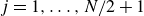$j=1,\dots ,N/2+1$ , to obtain $N/2+1$ equations for the unknown values $Y_{j}=Y (\zeta _{j} ), j=1,\dots ,N/2+1$ . Performing the discretization of the additional equations, (4.3)–(4.5), we can close the system for the N/2 + 4 unknowns $\tilde {c}$ , $\tilde {B}$ , $\tilde {d}$ and $Y_j$ , 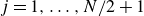$j=1,\dots ,N/2+1$ .

To solve the resulting nonlinear system of algebraic equations, we use the Levenberg–Marquardt algorithm implemented in the fsolve function of the Optimisation Toolbox of MATLAB. As an initial guess for this iterative procedure we use the first-order solution presented in § 3,

(4.7) \begin{align} \tilde {c}=C_0/\mu , \quad \quad \tilde {B}=0, \quad \quad \tilde {d}=1, \quad \quad Y(\zeta )=H \cos \left (\frac {2\pi }{L} \zeta \right ), \end{align}

where $H=\epsilon / \mu$ with our choice of scaling and $\epsilon$ is small. Unlike Ribeiro et al. (Reference Ribeiro, Milewski and Nachbin2017), who used the mean absolute residuals errors for the whole system of equations, our stopping criterion is based on the infinite norm of the residuals of (4.1). In our practice, with $N=128$ or $256$ both errors were found to be of the order $10^{-12}$ .

The following numerical results were obtained by natural numerical continuation in the parameters space, using the prior converged solution as the initial guess to a new solution. Owing to the number of dimensionless parameters characterizing branches of solutions, it is obviously a difficult task to give a thorough description of the bifurcation diagrams. Even in the simpler case of irrotational flows in deep water, namely with $\Omega =0$ and $\mu =\infty$ , Shelton et al. (Reference Shelton, Milewski and Trinh2021) have shown that the bifurcation space of the GC problem is certainly non-trivial, rendering difficult to observe any clear structure. Crucially, this is due to the existence of multiple solutions, the so-called Wilton ripples or combined waves, which emerge from resonant interactions between two modes. On account of this difficulty, we take $\mu$ and $\kappa$ as constants on a branch of solutions and vary $\Omega$ and $\epsilon$ over their admissible range in most of the cases studied here.

4.2. Gravity-capillary waves in irrotational flows

We first study irrotational flows with $\mu =10$ and several values of $\kappa$ . The values $\kappa =1$ and $0.8$ are taken to verify the correctness of the analytical solutions for GC waves, in which the effects of both gravity and capillarity are equally important, whereas the values of $\kappa =0.58,\,0.42$ and $0.30$ are used to determine the behaviour of the weakly nonlinear solutions close to the critical wavenumbers.

The variations of phase velocity $C$ as a function of $\epsilon$ for $\Omega =0$ and several values of $\kappa$ are shown in figure 5. The solid lines represent the numerical solutions of the Euler equations, and the dashed lines correspond to the approximate solutions. According to the asymptotic theory, the phase velocity decreases with the increase of $\epsilon$ for $\kappa =1,\,0.8$ and $0.58$ much like pure capillary waves, whereas it increases with $\epsilon$ for $\kappa =0.42$ and $0.30$ much like pure gravity waves. For $\kappa =1$ and $0.8$ the approximate solution agrees fairly well with the exact numerical solution over the range of $\epsilon$ values shown here. In contrast, with 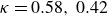$\kappa =0.58,\,0.42$ and $0.30$ the approximate solution matches the exact solution only for small values of the amplitude parameter $\epsilon$ .

Figure 5. Plot of phase velocity $C$ against $\epsilon$ for $\mu =10$ , $\Omega =0$ and some values of $\kappa =1.0,0.80,0.58, 0.42,0.30$ (from top to bottom): solid lines show the numerical results, dashed lines the analytical results and the boxed number indicates the type of the waves.

Figure 6. Plot of $C^2$ against $\kappa$ for $\mu =10$ , $\epsilon =0.10$ and $\Omega =0$ . Solid line, numerical solutions; dash–dotted line, weakly nonlinear analytical solution; dashed lines, infinitesimal wave solutions.

To better understand the meaning of the curves in figure 5, it should be realized that in general there is no unique branch of solutions for a fixed $\kappa$ , in the neighbourhood or not of the critical wavenumbers. This was demonstrated numerically by the seminal work of Schwartz & Vanden-Broeck (Reference Schwartz and Vanden-Broeck1979) in the deep-water case. With our numerical method and continuation in either the amplitude parameter $\epsilon$ or the surface tension parameter $\kappa$ , we find that this is also the case in finite depth, as illustrated by figure 6 where the variations of the squared phase velocity $C^2$ with $\kappa$ are shown.

In this figure three branches of numerical solutions with $\mu =10$ and $\epsilon =0.10$ are plotted with solid lines, as well as the corresponding weakly nonlinear solution (dash–dotted line obtained with (B11)) and the linear solutions for infinitesimal waves with (dimensional) wavenumber $nk_0$ for $n=1,\,2$ and $3$ (dashed lines obtained with (3.5)). According to the classification of the different branches of solutions proposed in Schwartz & Vanden-Broeck (Reference Schwartz and Vanden-Broeck1979), the types $1,\,2$ and $3$ are represented in this figure, and correspond to the number of observed ’dimples’ or inflexion points on a (half-) wave profile. Like in the deep-water case, for much of the figure the type number is seen to increase with $C^2$ for given $\kappa$ . For this value of the amplitude parameter, $\epsilon =0.10$ , the branches of types $1$ and $3$ follow the linear solution closely as $\kappa$ increases from the critical values $\kappa _1$ and $\kappa _2$ , respectively, whereas the wave profiles become indistinguishable from a sinusoid with wavenumbers $1$ and $3$ (in units of $k_0$ ), respectively. In contrast, the branch of type $2$ reaches a limiting configuration, as $\kappa$ increases, through the trapping of a bubble (not shown). As $\kappa \lt \kappa _1$ decreases, all the branches reach a limiting configuration through the trapping of one or more bubbles (not shown). As expected, the approximate solution for $C^2$ , the dash–dotted line in figure 6, breaks down as $\kappa$ approaches the critical value $\kappa _1$ . An interesting feature of this curve, however, is that for decreasing values of $\kappa \lt \kappa _1$ it approaches first the branch of type $2$ , and matches almost perfectly the branch of type $3$ when 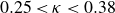$0.25\lt \kappa \lt 0.38$ .

Knowing that initialization of the numerical continuation method with the linear solution with $\kappa$ in the open intervals $[\kappa _{1},\infty]$ and $[\kappa _{n},\kappa _{n-1}]$ (with $n\geqslant 2$ ) yields numerical solutions corresponding to the branch of type $n$ , one can realize that, in figure 5, the branches with $\kappa =1,\,0.8$ and $0.58$ correspond to waves of type 1, while the branches with $\kappa =0.42$ and $0.30$ correspond to waves of the type $2$ and $3$ , respectively. This analysis is supported by the examination of typical surface profiles for several values of $\epsilon$ and $\kappa$ , as shown in figures 7 and 8.

Figure 7. Comparison of surface profiles between third-order (dotted line), fourth-order (dashed line) and exact numerical solutions (solid line) for $\Omega =0$ , $\mu =10$ and some values of $\epsilon =0.3, 0.2, 0.1$ (from top to bottom); (a) $\kappa =1$ , (b) $\kappa =0.8$ .

Figure 8. Comparison of surface profiles between third-order (dotted line), fourth-order (dashed line) and exact numerical solutions (solid line) for $\Omega =0$ , $\mu =10$ and some values of $\epsilon =0.1, 0.05, 0.025$ (from top to bottom); (a) $\kappa =0.58$ , (b) $\kappa =0.42$ , (c) $\kappa =0.30$ .

Figure 7 shows that the trough becomes deeper and narrower as $\kappa$ decreases from $1$ to $0.8$ and $\epsilon$ increases from $0.1$ to $0.3$ . It is to be noted that it displays only wave profiles corresponding to the type $1$ . For these waves where surface tension balances gravity, we observe that the fourth-order analytical solution provides better results than the third-order solution for predictions of the surface elevation and is in good agreement with the exact numerical solution when $\epsilon \le 0.2$ .

Figure 8 shows for smaller values of $\epsilon$ the surface profiles of near resonant waves with $\kappa =0.58,\,0.42$ and $0.30$ . For waves with $\kappa =0.58$ , figure 8(a) shows that the troughs tend to sharpen with the increase of $\epsilon$ , whereas the crests tend to flatten, which is typical of the waves of type $1$ . For the largest amplitude, $\epsilon =0.1$ , it is observed that the fourth-order solution makes a somewhat better job than the third-order solution, in the sense that it does not predict the formation of a crest dimple. Quantitatively, however, there is no significant improvement, neither near the crest nor near the trough. For waves with $\kappa =0.42$ the numerical solution indicates the presence of a secondary maximum on the surface profile with a trough between the two maxima, which is typical of the waves of type $2$ (see figure 8b ). For the largest amplitude, $\epsilon =0.1$ , neither of the asymptotic solutions is in agreement with the numerical solution. In fact, the fourth-order solution incorrectly predicts the occurrence of a crest dimple that is absent in the profiles of the third-order and numerical solutions. With $\kappa =0.30$ , the plots of figure 8(c) show that when the amplitude increases, the numerical solution takes the appearance of a primary sine wave with a relatively small $3$ -cycle perturbation superimposed upon it, which is typical of the waves of type $3$ . Similarly, neither of the asymptotic solutions is in agreement with the numerical solution for the largest amplitude considered here, though they predict qualitatively waves of type 3. It is noteworthy that when $\kappa$ is close to $\kappa _1$ , like in figures 8(a) and 8(b), the fourth-order approximations fail more importantly than the third-order ones for the larger steepness, due to the fact that the associated small divisors in (3.13)–(3.17) are found to be squared in the fourth-order coefficients.

Figure 9. Comparison of horizontal velocity profiles between third-order (dotted line), fourth-order (dashed line) and exact numerical solutions (solid line) for the waves plotted in figure 7(a). The profiles beneath the crest are plotted in (a), (c) and (e), and beneath the trough in (b), (d) and (f); and the steepness increases as (a,b) $\epsilon =0.1$ , (c,d) $\epsilon =0.2$ and (e,f) $\epsilon =0.3$ .

For further insight into the differences between the third- and fourth-order solutions, we have also compared the predictions of the interior flow with the numerical solutions. The method for the computation of the interior flow is explained in Ribeiro et al. (Reference Ribeiro, Milewski and Nachbin2017) and, therefore, need not be detailed here. To illustrate the differences in the interior flow, we have focused on the wave-induced horizontal velocities beneath the crest and the trough of the waves plotted in figure 7(a), where $\kappa =1$ is not close to $\kappa _1$ and $\epsilon =0.1,0.2$ and $0.3$ . Figure 9 shows the comparison between the asymptotic solutions and the exact results over the dimensionless range $y=-1$ to the free surface. Note that the bottom is located at $y=-10$ , where the wave-induced velocities vanish (not shown).

For the smallest steepness, it is found that the fourth-order predictions are closer to the exact results both beneath the crest and the trough. However, for the larger steepness the differences between the third-order and the fourth-order are much more important beneath the crest than beneath the trough. Actually, below the trough it is observed that those differences increase with the steepness and the fourth-order predictions are closer to the exact results. Beneath the crest, those differences also increase with the steepness, but neither such approximations are close to the exact results in the near surface region. Nonetheless, as the depth increases the fourth-order solutions are found to be better than the third-order ones. These results can be explained, noting that, firstly the local slopes at the trough are in closer agreement with the exact results than they are the crest, and secondly that a binomial expansion has been used in the dynamic boundary condition to approximate the nonlinear term related to the surface tension. Only two terms in this binomial expansion are required for the third-order approximation, but three terms are necessary for the fourth-order approximation. Due to this approximation there is a mismatch between the approximate wave-induced horizontal velocities and the exact results, though the differences in the phase velocity are very small over the range of steepness considered here (see figure 5, the case $\kappa =1$ ).

4.3. Gravity-capillary waves in flows with constant vorticity

Like in the previous subsection, we start by analysing the nonlinear dependency of the phase velocity on the wave steepness for the same different values of $\kappa$ but with different values of the vorticity parameter $\Omega$ . According to the numerical solutions the dependency of $C$ on $\epsilon$ is strongly affected by the vorticity whatever the value of $\kappa$ , as shown in figure 10. In comparison with the case of irrotational flow (see figure 5), not only the values of $C$ in the small amplitude limit are modified, but also the type of the waves depending on the value of $\kappa$ . In figure 10 the solid lines represent the numerical solutions of the Euler equations, and the dashed lines correspond to the approximate nonlinear dispersion relation presented in § 3. As expected from the linear dispersion relation (3.5), it is observed that in the limit of small amplitude increasing negative vorticity ( $\Omega \gt 0$ ) reduces the phase velocity, whereas increasing positive vorticity enhances it. In this limit the analytical results are in excellent agreement with the exact results whatever the value of $\kappa$ .

Figure 10. Plot of phase velocity $C$ against $\epsilon$ for $\mu =10$ and some values of $\kappa =1.0,0.80,0.58,0.42,0.30$ (from top to bottom): solid lines show the numerical results, dashed lines the analytical results and the boxed number indicates the type of the waves; (a) $\Omega =0.5$ , (b) $\Omega =0.9$ , (c) $\Omega =-0.5$ and (d) $\Omega =-0.9$ .

When $\Omega \gt 0$ , figures 10(a) and 10(b) show that for each value of $\kappa$ , the phase velocity is a decreasing function of the steepness. Except for the two lowest values of $\kappa$ , namely $0.30$ and $0.42$ , the agreement between the asymptotic theory and the exact theory is excellent over the range of steepness considered here, namely $0\lt \epsilon \le 0.25$ . In any case, the exact results, as well as the corresponding approximations, show that the phase velocity is a decreasing function of steepness. This suggests that the waves are capillary-like. For the calculations with $\kappa =0.30$ and $0.42$ , it appears that the mismatch between the approximations and the exact results is reduced with the increase of $\Omega$ , the curves becoming closer to each other over a larger range of steepness. In contrast, when $\Omega \lt 0$ the phase velocity is an increasing function of steepness for all $\kappa$ values, except for the branch of solutions with $\kappa =1$ and $\Omega =-0.5$ that is plotted as shown in figure 10(c). In this figure, the exact branches of solutions with $\kappa =1$ and $0.8$ agree with the approximations only when $\epsilon \lt 0.1$ . In figure 10(d), $\Omega =-0.9$ and the agreement between the approximations and the exact results is very satisfactory over the range of steepness shown here, namely $0\lt \epsilon \le 0.25$ .

To identify the type of waves for each branch of solutions plotted in figure 10 we may adopt the reasoning used in § 4.2 for the GC waves in irrotational flows. This in turn requires us to determine the critical values of $\kappa$ for given values of the intrinsic parameters $\tilde {h}$ and $\tilde {\Omega }$ . In our case $\mu =10$ and we have seen in § 3.2 that these critical values are mainly affected by the vorticity, the depth effects being negligible when $\tilde {h}\gg \tilde {h}_*$ . For each value of $\kappa$ and $\Omega$ used in figure 10, we have computed the first height $\kappa _n$ . These values are reported in table 1. It should be emphasized that for given values of $\mu$ and $\Omega$ , the intrinsic parameters $\tilde {h}$ and $\tilde {\Omega }$ have different values that depend on the value of $\kappa$ . The last column of table 1 indicates the type of the branch of solution for each triplet ( $\mu ,\,\kappa ,\,\Omega$ ) considered in figure 10. Solutions are of type $n+1$ when the values of $\kappa$ falls in the interval $[\kappa _{n+1},\kappa _n]$ for $n\geqslant 1$ . Waves of type 1 have wavelengths such that $\kappa \gt \kappa _1$ , where $\kappa _1$ is the largest critical wavenumber.

Table 1. Values of $\tilde {h}$ and $\tilde {\Omega }$ for given values of $\kappa$ and $\Omega$ . Here $\mu =10$ for each wave. The deep-water values of the first eight critical $\kappa _n$ are also reported, as well as the type of each wave.

Figure 11. Comparison of surface profiles and wave-induced horizontal velocity profiles under crest ( $u_c$ ) and trough ( $u_t$ ) for waves with $\mu =10, \,\Omega =0.5, \,\epsilon =0.10$ and several values of $\kappa$ . Third-order solution (dotted line), fourth-order solution (dashed line) and numerical solution (solid line): (a) $\kappa =1$ ; (b) $\kappa =0.80$ ; (c) $\kappa =0.58$ ; (d) $\kappa =0.42$ ; (e) $\kappa =0.30$ .

For several values of $\kappa$ and a fixed wave steepness, $\epsilon =0.10$ , we have also compared the surface profiles and the wave-induced horizontal velocities in the presence of a linear shear current with $\mu =10$ . Figure 11 shows the comparison between the analytical solutions and the exact results for waves of different wavelengths, namely $\kappa =1,\,0.80,\,0.58,\,0.42$ and $0.30$ , and a vorticity parameter $\Omega =0.5$ . According to table 1 all the waves are of type $1$ , since their wavelength is such that $\kappa \gt \kappa _1$ . Except for the longest wave with $\kappa =0.30$ , there is a remarkable agreement between the analytical results and the exact ones, the fourth-order results being more accurate than the third-order ones. As expected, neither such approximations is valid for the waves with $\kappa =0.30$ , a value that is very close to $\kappa _1\approx 0.27$ .

Figure 12. Same legend as in figure 11 but with $\Omega =-0.5$ .

The same comparison has been carried out with $\Omega =-0.5$ , and the results are shown in figure 12. According to table 1, each wave is of a different type. The type number is seen to increase with increasing wavelength. The shortest wave ( $\kappa =1$ ) is the only capillary-like wave, in the sense that it belongs to a branch of solutions with decreasing phase velocity with increasing steepness (see figure 10 c), and it is of type $1$ as shown in figure 12(a). Again, for this value of $\kappa$ that is close to the $\kappa _1\approx 0.92$ , both the third-order and fourth-order solutions differ significantly from the exact results, the disagreement being larger near the crest than near the trough. For the wave of type $2$ shown in figure 12(b) we have $\kappa =0.80$ , which falls near the middle of the interval $[\kappa _2,\kappa _1]=[0.61,0.90]$ . Looking at the wave-induced horizontal velocities, it is found that the fourth-order theory does a better job than the third-order one beneath the trough, and that the situation is reversed beneath the crest. Nonetheless, both analytical solutions fail to match with the exact results in the near surface region. Actually, these differences between the exact results and the approximations are expected in view of figure 10(c), which shows that there is mismatch in the prediction of $C$ for the waves with $\kappa =1$ and $0.80$ .

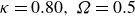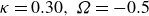Figure 13. Comparison of surface profiles and wave-induced horizontal velocity profiles under crest ( $u_c$ ) and trough ( $u_t$ ) for waves with $\mu =10, \,\epsilon =0.20$ . Third-order solution (dotted line), fourth-order solution (dashed line) and numerical solution (solid line): (a) $\kappa =1,\,\Omega =0.5$ ; (b) $\kappa =0.80,\,\Omega =0.5$ ; (c) $\kappa =0.42,\,\Omega =-0.5$ ; (d) $\kappa =0.30,\,\Omega =-0.5$ .

In contrast, for the gravity-like waves with $\kappa =0.58,\,0.42$ and $0.30$ , figure 10(c) shows an excellent agreement between the exact phase velocity and the approximate one when $\epsilon =0.1$ . Not surprisingly, when the value of $\kappa$ is close to one of the first three critical values $\kappa _n$ , both approximations fail to reproduce the near surface horizontal velocities (see figures 12 c and 12 d). However, when $\kappa =0.42$ we have $|\kappa -\kappa _2|=0.15$ , $|\kappa -\kappa _3|=0.01$ , and although the approximate surface profiles are almost indistinguishable from the exact solution, it is found that there are important differences in the internal flow structure. Figure 12(d) shows that the fourth-order theory does a better job than the third-order one beneath the trough, the situation being reversed beneath the crest. As shown in figure 12(e), the surface profiles and the wave-induced horizontal velocities are indistinguishable from the exact solution for the wave with $\kappa =0.32$ , which is in the interval $[\kappa _5,\kappa _4]$ and far enough the smallest critical value of either the third-order or fourth-order approximations.

Finally we present the results of a similar comparison for steeper waves with $\mu =10,\,\Omega =\pm 0.5$ and $\epsilon =0.2$ . The four different waves have been chosen so that the approximation of the phase velocity is still in very good agreement with the exact solution. In view of the results of figures 10(a) and 10(c), we consider $\kappa =1$ and $\kappa =0.8$ with $\Omega =0.5$ , whereas with $\Omega =-0.5$ we choose $\kappa =0.42$ and $\kappa =0.30$ . For the waves with $\Omega =0.5$ , $\kappa$ is quite far from the first critical value $\kappa _1$ , and we observe that the third- and fourth-order surface profiles are almost indistinguishable from the exact solution. However, in each case the approximations fail to describe the wave-induced velocities close to the surface. Nonetheless it should be noticed that the fourth-order solution performs better than the third-order one, though this improvement is lessened beneath the crest. For the waves with $\Omega =-0.5$ and $\kappa =0.42$ , which falls in $[\kappa _4,\kappa _3]=[0.35,0.43]$ , figure 13(c) shows that nonlinearity has become sufficiently important to reveal the defect of the fourth-order theory in comparison with the third-order theory and the exact results (see also for comparison figure 12 d). For the longest wave with $\kappa =0.30$ , shown in figure 13(d), the approximate surface profiles are in very good agreement with the exact results. In this case the coefficients of the asymptotic series are well ordered, $\kappa$ being $O(\epsilon )$ far from $\kappa _1=0.80,\,\kappa _2=0.55$ and $\kappa _3=0.42$ , though they fail to predict the wave-induced velocities close to the surface beneath both crest and trough. Actually there is no improvement using the fourth-order theory and its results are very similar to that obtained with the third-order theory.