


1. Introduction
Surface-tension-driven phenomena in pure simple-liquid systems are ubiquitous in nature, as well as in industrial applications. For example, tears of wine (Scriven & Sternling Reference Scriven and Sternling1960), the footprint of a whale caused by the sweeping of the biomaterial to the surface (Levy et al. Reference Levy, Uminsky, Park and Calambokidis2011), crystal growth techniques (Schwabe et al. Reference Schwabe, Scharmann, Preisser and Oeder1978) and in experiments with heated fluid layers in microgravity (Smith & Davis Reference Smith and Davis1983a , Reference Smith and Davisb ; Schatz & Neitzel Reference Schatz and Neitzel2001) are some of these, just to mention a few. The inhomogeneity of scalar fields at the layer interface such as temperature that affects the local surface tension may induce, under certain conditions, a convective motion in a liquid layer, known in the literature as the Marangoni or thermocapillary instability (Davis Reference Davis1987). Pearson (Reference Pearson1958) was the first to theoretically investigate the onset of the monotonic Marangoni instability, which may be either long-wave or short-wave, by considering a layer of a pure Newtonian liquid with the non-deformable interface which is heated at its solid support, provided that the temperature drop across the layer is sufficiently large to overcome the dissipative properties of the liquid such as viscosity and thermal diffusivity. Scriven & Sternling (Reference Scriven and Sternling1964) later found that interfacial deflection significantly alters the stability boundary and may lead to the onset of the oscillatory Marangoni instability. However, their result was further corrected by Smith (Reference Smith1966) who showed the stabilisation of the long-wave gravitational waves predicted by Scriven & Sternling (Reference Scriven and Sternling1964). In a similar way, in an isothermal fluid layer, inhomogeneities of the local solute concentration at the layer interface also affect the local surface tension and may lead to the emergence of the solutocapillary instability (Davies & Rideal Reference Davies and Rideal1963).
In a pure liquid layer, heating at the layer interface or, equivalently, cooling at the substrate, provides a stabilising mechanism (Deissler & Oron Reference Deissler and Oron1992; Oron & Rosenau Reference Oron and Rosenau1992; Alexeev & Oron Reference Alexeev and Oron2007), which may lead to a full stabilisation or saturation at the nonlinear stage. The suppression of the Rayleigh–Taylor instability in an inverted air–oil system by the thermocapillarity was demonstrated experimentally by Burgess et al. (Reference Burgess, Juel, McCormick, Swift and Swinney2001).
In liquid mixtures such as binary mixtures, the Soret effect (Cross & Hohenberg Reference Cross and Hohenberg1993; Skarda, Jacqmin & McCaughan Reference Skarda, Jacqmin and McCaughan1998) introduces an additional component to the expression of Fick’s law for the mass flux normally related to the gradient of the bulk solute concentration. It is associated with the temperature gradient in the mixture and is found to be important. By coupling between heat and mass transfer effects, the Soret effect by itself may affect and modify thermal instabilities in a layer of a binary mixture (Oron & Nepomnyashchy Reference Oron and Nepomnyashchy2004). Various aspects of long- and finite-wave thermosolutocapillary instabilities in dilute binary mixtures heated at the substrate have already been investigated (Oron & Nepomnyashchy Reference Oron and Nepomnyashchy2004; Podolny, Oron & Nepomnyashchy Reference Podolny, Oron and Nepomnyashchy2005; Shklyaev et al. Reference Shklyaev, Nepomnyashchy and Oron2007, Reference Shklyaev, Nepomnyashchy and Oron2009; Bestehorn & Borcia Reference Bestehorn and Borcia2010; Podolny, Nepomnyashchy & Oron Reference Podolny, Nepomnyashchy and Oron2010; Morozov, Oron & Nepomnyashchy Reference Morozov, Oron and Nepomnyashchy2014). Sarma & Mondal (Reference Sarma and Mondal2021a ) studied thermosolutocapillary instabilities in a viscoelastic binary fluid with a particular case of a Newtonian binary fluid at zero Deborah number. In all of these papers, the emergence of both monotonic and oscillatory instabilities was reported.
The instability mechanism for such a system depends on the direction of heating or cooling. Joo (Reference Joo1995) revealed the onset of the monotonic solutocapillary instability in a layer of a binary mixture with heating imposed at the free interface. Furthermore, it was noted that oscillatory instability takes place due to the competition between the stabilising solutocapillary and destabilising thermocapillary instability in the case of heating at the substrate (Joo Reference Joo1995). Sarma & Mondal (Reference Sarma and Mondal2021b ) investigated thermosolutal Marangoni instability in a layer of a viscoelastic binary fluid heated at the interface. They showed the emergence of a long-wave monotonic instability in the cases of both a deformable and non-deformable layer interface, and demonstrated that this instability is driven by solutocapillarity.
Colloidal dispersions made of a mixture of a base fluid and nanoparticles of diameter $d_p^*$
between
$d_p^*$
between $1$
and
$1$
and $100$
nm are known as nanofluids. The material properties of a nanofluid such as density, kinematic viscosity, thermal diffusivity and Soret diffusion coefficient naturally depend on the local bulk concentration of the particles (Buongiorno Reference Buongiorno2006), as well as the Brownian diffusion coefficient (Batchelor Reference Batchelor1976). This fact introduces obvious challenges affecting theoretical work and practical applications such as inkjet printing (Lohse Reference Lohse2022), paint coating and microgravity experiments (Vailati et al. Reference Vailati2023). In heat-transfer related technological applications, metallic particles, for instance, alumina, copper oxide, silica, titania, etc., are purposely employed to enhance the thermal conductivity of the nanofluid relative to that of the base fluid (Choi & Eastman Reference Choi and Eastman1995). There are also promising technological applications such as nanofluid fuel (Abramzon & Sirignano Reference Abramzon and Sirignano1989; Basu & Miglani Reference Basu and Miglani2016), where thermosolutal Marangoni stresses are of importance (Vang & Shaw Reference Vang and Shaw2020; Shaw Reference Shaw2022). The thermophysical stratification in such systems introduces even more complex features into mathematical modelling and investigations due to that.
$100$
nm are known as nanofluids. The material properties of a nanofluid such as density, kinematic viscosity, thermal diffusivity and Soret diffusion coefficient naturally depend on the local bulk concentration of the particles (Buongiorno Reference Buongiorno2006), as well as the Brownian diffusion coefficient (Batchelor Reference Batchelor1976). This fact introduces obvious challenges affecting theoretical work and practical applications such as inkjet printing (Lohse Reference Lohse2022), paint coating and microgravity experiments (Vailati et al. Reference Vailati2023). In heat-transfer related technological applications, metallic particles, for instance, alumina, copper oxide, silica, titania, etc., are purposely employed to enhance the thermal conductivity of the nanofluid relative to that of the base fluid (Choi & Eastman Reference Choi and Eastman1995). There are also promising technological applications such as nanofluid fuel (Abramzon & Sirignano Reference Abramzon and Sirignano1989; Basu & Miglani Reference Basu and Miglani2016), where thermosolutal Marangoni stresses are of importance (Vang & Shaw Reference Vang and Shaw2020; Shaw Reference Shaw2022). The thermophysical stratification in such systems introduces even more complex features into mathematical modelling and investigations due to that.
It is important to note that instabilities may also be triggered in a simple fluid layer featuring a non-uniformity in one or more of the physical properties of the fluid. For instance, if the fluid density in a horizontal layer in the gravity field increases with height, a situation where a heavier fluid is above the lighter one, the system may become unstable (Rayleigh Reference Rayleigh1882; Chandrasekhar Reference Chandrasekhar1961). An analogue to this instability may arise in a nanofluid layer due to the presence of nanoparticles heavier than the carrier liquid in its upper stratum. We refer to this instability as to the solutal buoyancy instability since the local density of the fluid depends on the local particle concentration. The presence of the Soret effect with a positive thermodiffusivity coefficient promotes the formation of an unstable nanoparticle concentration stratification across the layer, and thereby enhances the possibility of the onset of the solutal buoyancy instability. Although off the scope of the current paper, in liquid metal batteries (Herreman et al. Reference Herreman, Bénard, Nore, Personnettaz, Cappanera and Guermond2020), the onset of the solutal buoyancy instability during the charge phase was found due to the emergence of the unstable stratification of lithium. Interestingly, Herreman et al. (Reference Herreman, Bénard, Nore, Personnettaz, Cappanera and Guermond2020) found that the onset of solutal buoyancy convection actually helps to homogenise the alloy layer, and the same physical effect introduces complexities during the discharge phase by creating the stable stratification (Herreman et al. Reference Herreman, Nore, Cappanera and Guermond2021). Solutal buoyancy instability was also found to create convective flow by dissolution from a soluble solid into a fluid (Berhanu et al. Reference Berhanu, Philippi, Courrech du Pont and Derr2021).
Furthermore, the viscosity of a nanofluid increases with the local particle concentration and can be approximated via an empirical model (Maron & Pierce Reference Maron and Pierce1956). We note that in shear-induced flows, additional contributions to the normal stress in a nanofluid may be important in the presence of a base flow (Phillips et al. Reference Phillips, Armstrong, Brown, Graham and Abbott1992; Dhas & Roy Reference Dhas and Roy2022; Lavrenteva, Smagin & Nir Reference Lavrenteva, Smagin and Nir2024), but in the case considered in the current paper, the base state is quiescent, and hence, these effects may be safely omitted.
Experimental data show that the thermal conductivity of a nanofluid varies with the local particle concentration. Maxwell (Reference Maxwell1873) and Jeffrey (Reference Jeffrey1973) derived analytical expressions for the thermal conductivity of a suspension of spherical particles in a fluid. Buongiorno (Reference Buongiorno2006) proposed analytical expressions based on experimental data for this feature for two cases of nanofluids, namely those of alumina particles in water and titanium particles in water. It is interesting to note that thermal conductivity stratification in a two-layer system of Newtonian fluids may significantly influence its stability. For instance, Welander (Reference Welander1964) and Gershuni & Zhukhovitskii (Reference Gershuni and Zhukhovitskii1980) investigated the onset of an oscillatory instability induced by the thermal conductivity stratification in a stably stratified two-layer liquid system. Such instability may be driven by a disparity between the characteristic diffusion time scales of the two liquids.
The purpose of this paper is to investigate the combined thermo-solutocapillary instability in a layer of a moderately dense nanoparticle suspension subjected to the Soret effect, bounded by a deformable liquid–gas interface and supported by a horizontal solid substrate subjected to a prescribed heat flux in the gravity field. The cases of both heating and cooling at the substrate are considered. To simplify the analysis, we assume the carrier fluid to be a simple Newtonian liquid. In contradistinction with the Rayleigh–Bénard instability in a nanofluid layer considered by Chang & Ruo (Reference Chang and Ruo2022), the thermosolutocapillary instability in nanofluids has not been investigated to date. The main challenge and the novelty of the current investigation is taking into account the dependence of all thermophysical properties of the nanofluid on the local particle concentration, which was not considered before in this context, e.g., by Chang & Ruo (Reference Chang and Ruo2022). In our approach, because of the dependence of the fluid density on the local particle concentration which varies within the bulk, we adopt a ‘compressible’ approach to describe the dynamics of a nanofluid and show that the contribution of ‘compressibility’ is minor. As a result of accounting for the dependence of the thermophysical properties on the local particle concentration, we find that in the case of a layer heated at the substrate, such variation of thermal conductivity of the fluid leads to the change of the instability type from monotonic for weak variations to oscillatory for stronger variations. In the case of the layer cooled at the substrate, the emerging instability is monotonic, similar to what Sarma & Mondal (Reference Sarma and Mondal2021b ) found for a Newtonian dilute binary fluid. Most of the instabilities found in this investigation are finite-wave, although narrow windows of long-wave instability also emerge in both cases of the heating direction.
The plan of the paper is as follows. Section 2 offers the problem formulation, and presents a set of governing equations and boundary conditions accounting for local particle concentration-dependent thermophysical properties of the system. The quiescent base state of the system is presented in § 2.4 with the details of its derivation given in Appendix A.1. Section 3 is dedicated to the linear stability analysis of the determined base state and presents the eigenvalue problem which is numerically investigated. Section 4, subdivided into six subsections, presents the results of the investigation: § 4.1 outlines the numerical procedure used for solving the linear eigenvalue problem; § 4.2 presents the results for the case of cooling at the substrate; whereas § 4.3 delivers the results for the case of heating at the substrate. Further, §§ 4.4, 4.5 and 4.6 explore the effect of the thermal conductivity stratification of the suspension on the system instability, presents typical eigenfunctions corresponding to the observed instabilities and discusses a possibility of using an incompressibility simplification, which is akin, in some sense, to the Boussinesq approximation for a heated layer of a simple liquid, respectively. A use of a simplified ‘incompressible’ formulation could significantly reduce the numerical effort associated with the solution of the linear eigenvalue problem in its full formulation. Finally, § 5 summarises the findings of the paper.
2. Problem formulation and governing equations
We consider a nanofluid layer of a mean thickness $h_0^\ast$
, density
$h_0^\ast$
, density $\rho ^\ast _{nf}$
, dynamic viscosity
$\rho ^\ast _{nf}$
, dynamic viscosity $\mu ^\ast _{nf}$
, kinematic viscosity
$\mu ^\ast _{nf}$
, kinematic viscosity $\nu ^\ast _{nf}=\mu ^\ast _{nf}/\rho ^\ast _{nf}$
, thermal conductivity
$\nu ^\ast _{nf}=\mu ^\ast _{nf}/\rho ^\ast _{nf}$
, thermal conductivity $K^\ast _{nf}$
, heat capacity
$K^\ast _{nf}$
, heat capacity $c^\ast _{nf}$
, and thermal diffusivity
$c^\ast _{nf}$
, and thermal diffusivity $\kappa ^\ast _{nf} = K^\ast _{nf}/\rho ^\ast _{nf} c^\ast _{nf}$
. Here, the subscripts
$\kappa ^\ast _{nf} = K^\ast _{nf}/\rho ^\ast _{nf} c^\ast _{nf}$
. Here, the subscripts $nf$
refer to the nanofluid. In what follows, the presence of nanoparticles in a nanofluid will be accounted for via the local concentration of particles.
$nf$
refer to the nanofluid. In what follows, the presence of nanoparticles in a nanofluid will be accounted for via the local concentration of particles.
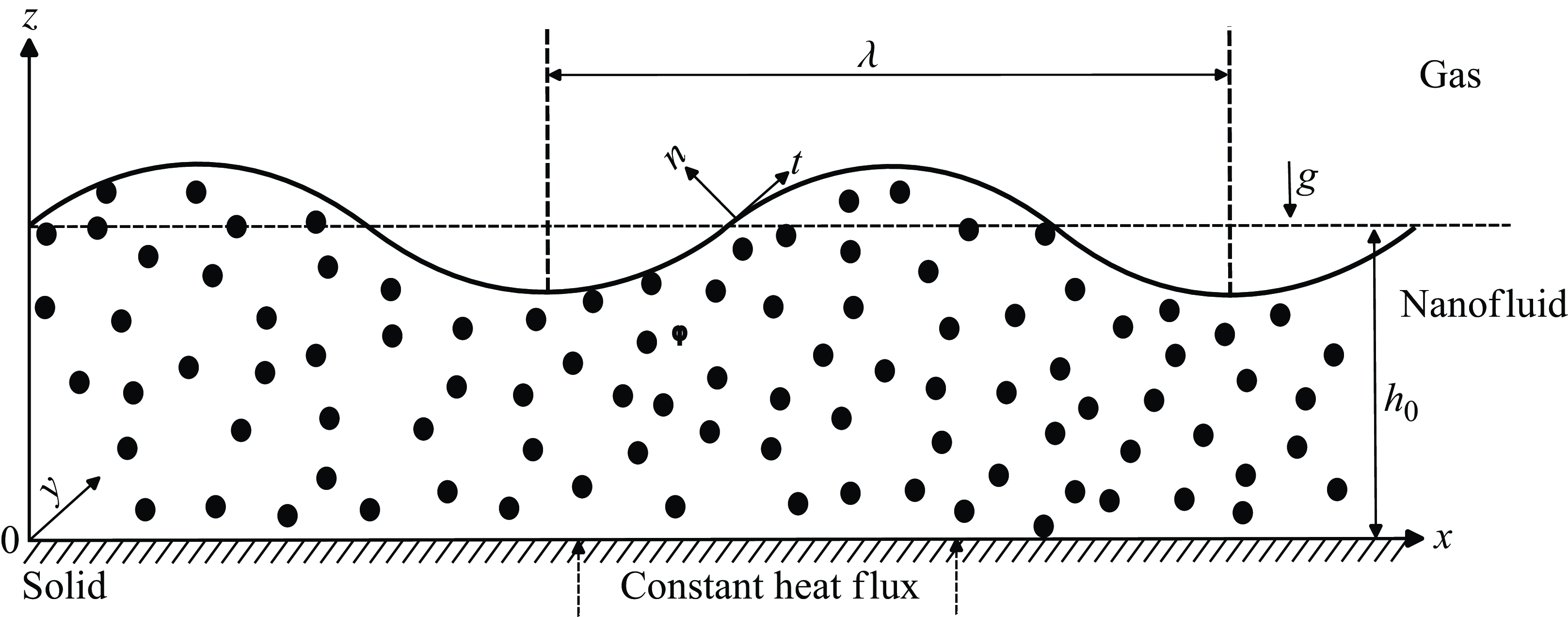
Figure 1. Nanofluid $(d_p^*=10{-}100\,\text{nm})$
layer on the solid substrate subjected to a constant heat flux at the substrate and exposed to the gas phase at its deformable interface.
$(d_p^*=10{-}100\,\text{nm})$
layer on the solid substrate subjected to a constant heat flux at the substrate and exposed to the gas phase at its deformable interface.
We further denote the physical properties of the base fluid and the nanoparticles with subscripts $bf$
and
$bf$
and $np$
, respectively. The nanofluid layer is assumed to be of local thickness
$np$
, respectively. The nanofluid layer is assumed to be of local thickness $h^\ast$
and rests on a solid planar horizontal substrate being exposed at its deformable liquid–gas interface to the quiescent gas environment held at constant pressure
$h^\ast$
and rests on a solid planar horizontal substrate being exposed at its deformable liquid–gas interface to the quiescent gas environment held at constant pressure $p^\ast _\infty$
and temperature
$p^\ast _\infty$
and temperature $T_\infty ^*$
in the gravity field
$T_\infty ^*$
in the gravity field $g^*$
. The frame of reference is chosen so that the
$g^*$
. The frame of reference is chosen so that the $x^\ast$
and
$x^\ast$
and $y^\ast$
axes are located in the substrate, whereas the axis
$y^\ast$
axes are located in the substrate, whereas the axis $z^\ast$
is normal to the substrate and directed into the fluid layer opposite to the direction of gravity; hence, the substrate and the deformable liquid–gas interface are located at
$z^\ast$
is normal to the substrate and directed into the fluid layer opposite to the direction of gravity; hence, the substrate and the deformable liquid–gas interface are located at $z^\ast =0$
and
$z^\ast =0$
and $z^\ast =h^\ast$
, respectively (figure 1).
$z^\ast =h^\ast$
, respectively (figure 1).
The fluid is assumed to be a moderately dense nanofluid, i.e. a mixture of a Newtonian base fluid with nanoparticles of $d_p^\ast \approx 10 \,\text{nm}$
whose volumetric concentration
$d_p^\ast \approx 10 \,\text{nm}$
whose volumetric concentration $\phi ^\ast = \phi ^\ast (x^\ast, y^\ast, z^\ast, t^\ast )$
is varying in time
$\phi ^\ast = \phi ^\ast (x^\ast, y^\ast, z^\ast, t^\ast )$
is varying in time $t^\ast$
and space. The entire system is subjected to the prescribed heat flux
$t^\ast$
and space. The entire system is subjected to the prescribed heat flux $\mathcal{Q}q^\ast$
with
$\mathcal{Q}q^\ast$
with $\mathcal{Q}=\pm 1$
and
$\mathcal{Q}=\pm 1$
and $q^\ast \gt 0$
at its solid bottom in the direction normal to the latter. Note that the value of
$q^\ast \gt 0$
at its solid bottom in the direction normal to the latter. Note that the value of $\mathcal{Q}$
is related to the direction of the heat flux, so that the cases of
$\mathcal{Q}$
is related to the direction of the heat flux, so that the cases of $\mathcal{Q}=1$
and
$\mathcal{Q}=1$
and $\mathcal{Q}=-1$
correspond to heating and cooling at the solid–liquid interface, respectively. An imposed heat flux leads to the emergence of the temperature field
$\mathcal{Q}=-1$
correspond to heating and cooling at the solid–liquid interface, respectively. An imposed heat flux leads to the emergence of the temperature field $T^\ast =T^\ast (x^\ast, y^\ast, z^\ast, t^\ast )$
varying with time and space within the layer.
$T^\ast =T^\ast (x^\ast, y^\ast, z^\ast, t^\ast )$
varying with time and space within the layer.
The surface tension at the liquid–gas interface is assumed to depend on both the interfacial temperature and nanoparticle concentration, and for small variations of temperature and particle concentration at the interface, is adequately approximated by a linear function
 \begin{equation} \sigma ^\ast (T^\ast, \phi ^\ast ) = \sigma ^\ast _r - \sigma ^\ast _{T^\ast }(T^\ast -T_r^\ast )-\sigma ^\ast _{\phi ^\ast }(\phi ^\ast -\phi _r^\ast ), \end{equation}
where
 \begin{equation} \sigma ^\ast _{T^\ast } = -\partial \sigma ^\ast /\partial T^\ast \gt 0\quad \text{and}\quad \sigma _{\phi ^\ast }^\ast = -\partial \sigma ^\ast /\partial \phi ^\ast \gt 0. \end{equation}
Here, $\sigma ^\ast _r$
is the equilibrium reference value of the surface tension at the reference values of
$\sigma ^\ast _r$
is the equilibrium reference value of the surface tension at the reference values of $T_r^\ast$
and
$T_r^\ast$
and $\phi _r^\ast$
, so
$\phi _r^\ast$
, so $\sigma ^\ast _r=\sigma ^\ast (T_r^\ast, \phi _r^\ast )$
, and both
$\sigma ^\ast _r=\sigma ^\ast (T_r^\ast, \phi _r^\ast )$
, and both $\sigma ^\ast _{T^\ast }$
and
$\sigma ^\ast _{T^\ast }$
and $\sigma ^\ast _{\phi ^\ast }$
are positive, thus, the surface tension linearly decreases with both the temperature and particle concentration at the interface. We use, as an example, an alumina nanoparticle dispersion in distilled water which exhibits a vanishing value of the adsorption/desorption coefficient ratio; hence, it is possible to neglect interfacial kinetics mechanisms in this situation. However, we note that nanoparticle dispersions in different liquids such as non-stabilised water, n-decane, n-dodecane, n-hexadecane, etc., exhibit a significant contribution of the interfacial kinetics. In those cases, consideration of the interfacial kinetics becomes necessary (Machrafi Reference Machrafi2022), and instead of the interfacial value of the bulk particle concentration
$\sigma ^\ast _{\phi ^\ast }$
are positive, thus, the surface tension linearly decreases with both the temperature and particle concentration at the interface. We use, as an example, an alumina nanoparticle dispersion in distilled water which exhibits a vanishing value of the adsorption/desorption coefficient ratio; hence, it is possible to neglect interfacial kinetics mechanisms in this situation. However, we note that nanoparticle dispersions in different liquids such as non-stabilised water, n-decane, n-dodecane, n-hexadecane, etc., exhibit a significant contribution of the interfacial kinetics. In those cases, consideration of the interfacial kinetics becomes necessary (Machrafi Reference Machrafi2022), and instead of the interfacial value of the bulk particle concentration $\phi ^\ast$
, a surface particle concentration
$\phi ^\ast$
, a surface particle concentration $\Gamma ^*$
needs to be used in (2.1a
) and (2.1b
).
$\Gamma ^*$
needs to be used in (2.1a
) and (2.1b
).
2.1. Thermophysical properties of a nanofluid
In the case of non-dilute mixtures, the thermophysical properties of a nanofluid depend on the local particle concentration (Buongiorno Reference Buongiorno2006). The density and the specific heat capacity of a nanofluid are determined as the weighted sum of the respective properties of the base fluid and the nanoparticles,
 \begin{align}&\qquad \rho ^\ast _{nf}(\phi ^\ast ) =(1-\phi ^\ast )\rho ^\ast _{bf}+\phi ^\ast \rho ^\ast _{np}, \end{align}
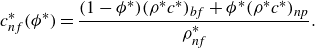 \begin{align}& c^\ast _{nf}(\phi ^\ast ) = \frac {(1-\phi ^\ast )(\rho ^\ast c^\ast ) _{bf}+ \phi ^\ast (\rho ^\ast c^\ast ) _{np}}{\rho _{nf}^\ast }. \end{align}
The thermal conductivity of nanofluids is also known to depend on the local particle concentration. In what follows, we use the empirical model
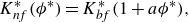 \begin{equation} K^\ast _{nf}(\phi ^\ast ) = K^\ast _{bf}(1 + a \phi ^\ast ), \end{equation}
where $a$
is a constant describing the degree of the thermal conductivity variation with the local particle concentration. The value
$a$
is a constant describing the degree of the thermal conductivity variation with the local particle concentration. The value $a=7.47$
(Buongiorno Reference Buongiorno2006) is valid for an alumina
$a=7.47$
(Buongiorno Reference Buongiorno2006) is valid for an alumina $\text{Al}_2\text{O}_3$
nanoparticles suspension in water. This value was extracted from the experimental data of Pak & Cho (Reference Pak and Cho1998) who measured thermal conductivity of an alumina–water nanofluid for various particle concentrations. The relationship between the thermal conductivity of the nanofluid and the particle concentration depends on both particles and solvent material. For instance, in the case of titania nanoparticles in water, the thermal conductivity varies with the particle concentration as
$\text{Al}_2\text{O}_3$
nanoparticles suspension in water. This value was extracted from the experimental data of Pak & Cho (Reference Pak and Cho1998) who measured thermal conductivity of an alumina–water nanofluid for various particle concentrations. The relationship between the thermal conductivity of the nanofluid and the particle concentration depends on both particles and solvent material. For instance, in the case of titania nanoparticles in water, the thermal conductivity varies with the particle concentration as
 \begin{align} K^\ast _{nf}(\phi ^\ast ) = K^\ast _{bf} (1+2.92\phi ^\ast -11.99\phi ^{\ast 2}) \end{align}
(Buongiorno Reference Buongiorno2006).
We note that in the absence of an empirical relationship between the thermal conductivity $K^\ast _{nf}$
of a nanosuspension and its particle concentration
$K^\ast _{nf}$
of a nanosuspension and its particle concentration $\phi ^\ast$
, one can employ the analytical models developed by Maxwell (Reference Maxwell1873) and Jeffrey (Reference Jeffrey1973), which estimated the value of
$\phi ^\ast$
, one can employ the analytical models developed by Maxwell (Reference Maxwell1873) and Jeffrey (Reference Jeffrey1973), which estimated the value of $K^\ast _{nf}$
for a dilute (
$K^\ast _{nf}$
for a dilute ( $\phi ^\ast /\phi _m \ll 1$
with
$\phi ^\ast /\phi _m \ll 1$
with $\phi _m$
being the maximal packing volume fraction) suspension providing terms proportional to
$\phi _m$
being the maximal packing volume fraction) suspension providing terms proportional to $\phi ^\ast$
, whose coefficient could have yielded the value of
$\phi ^\ast$
, whose coefficient could have yielded the value of $a$
, and
$a$
, and $ (\phi ^\ast )^2$
, respectively. Our estimate for the value of
$ (\phi ^\ast )^2$
, respectively. Our estimate for the value of $a$
, based on Maxwell theory and the values of thermal conductivity of Al
$a$
, based on Maxwell theory and the values of thermal conductivity of Al $_2$
O
$_2$
O $_3$
and water, yields
$_3$
and water, yields $a \lesssim 3$
, which is quite far from the experimental value of
$a \lesssim 3$
, which is quite far from the experimental value of $a=7.47$
; therefore, in most of our results presented below,
$a=7.47$
; therefore, in most of our results presented below, $a=7.47$
is adopted. Additionally, we mention that the limits of the effective thermal conductivity
$a=7.47$
is adopted. Additionally, we mention that the limits of the effective thermal conductivity $(K_{nf}^*/K_{bf}^*)$
of a monodisperse nanosuspension can be estimated by the Hashin–Shtrikman bounds (Hashin & Shtrikman Reference Hashin and Shtrikman1962; Keblinski, Prasher & Eapen Reference Keblinski, Prasher and Eapen2008)
$(K_{nf}^*/K_{bf}^*)$
of a monodisperse nanosuspension can be estimated by the Hashin–Shtrikman bounds (Hashin & Shtrikman Reference Hashin and Shtrikman1962; Keblinski, Prasher & Eapen Reference Keblinski, Prasher and Eapen2008)
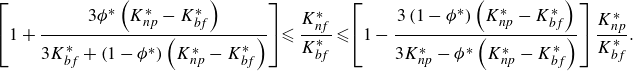 \begin{align} \left [1+\frac {3\phi ^*\left (K_{np}^*-K_{bf}^*\right )}{3K_{bf}^*+\left (1-\phi ^*\right )\left (K_{np}^*-K_{bf}^*\right )}\right ]\!\leqslant \frac {K_{nf}^*}{K_{bf}^*}\leqslant \!\left [1-\frac {3\left (1-\phi ^*\right )\left (K_{np}^*-K_{bf}^*\right )}{3K_{np}^*-\phi ^*\left (K_{np}^*-K_{bf}^*\right )}\right ]\frac {K_{np}^*}{K_{bf}^*}. \end{align}
We find that in a low-concentration limit $\phi ^*\ll 1$
, the effective thermal conductivity parameter
$\phi ^*\ll 1$
, the effective thermal conductivity parameter $a$
for Al
$a$
for Al $_2$
O
$_2$
O $_3$
nanoparticles in water ranges therefore in the interval
$_3$
nanoparticles in water ranges therefore in the interval $2.84\leqslant a\leqslant 38$
. Also, the effect of varying
$2.84\leqslant a\leqslant 38$
. Also, the effect of varying $a$
on the properties of the instability will be briefly assessed in § 4.4.
$a$
on the properties of the instability will be briefly assessed in § 4.4.
As for the nanofluid viscosity, we employ the empirical correlation model proposed by Maron & Pierce (Reference Maron and Pierce1956) and de Kruif et al. (Reference de Kruif, van Iersel, Vrij and Russel1985) for a concentrated suspension,
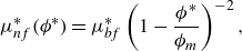 \begin{equation} \mu ^\ast _{nf}(\phi ^\ast ) = \mu ^\ast _{bf} \left (1-\frac {\phi ^\ast }{\phi _m}\right )^{-2}, \end{equation}
where $\phi _m$
is the maximal packing fraction. The value of
$\phi _m$
is the maximal packing fraction. The value of $\phi _m$
varies from
$\phi _m$
varies from $0.524\ \text{to}\ 0.71$
. We use the value of
$0.524\ \text{to}\ 0.71$
. We use the value of $\phi _m=0.65$
related to the random close packing (RCP) volume fraction of nanoparticles. The viscosity model given by (2.2f
) illustrates the power-law variation of the viscosity with the nanoparticle concentration growing indefinitely when the nanoparticle concentration
$\phi _m=0.65$
related to the random close packing (RCP) volume fraction of nanoparticles. The viscosity model given by (2.2f
) illustrates the power-law variation of the viscosity with the nanoparticle concentration growing indefinitely when the nanoparticle concentration $\phi ^\ast \to \phi _m$
.
$\phi ^\ast \to \phi _m$
.
2.2. Physical mechanisms relevant for our model
Buongiorno (Reference Buongiorno2006) described seven different slip mechanisms, i.e. mechanisms causing deviation of the particle velocity field from that of the carrier fluid, for the nanoparticle motion in a nanofluid. Out of these seven, we account for the two dominant slip mechanisms, namely, the Brownian and the Soret diffusion (thermophoresis).
The Brownian diffusion coefficient is given by the generalised Stokes–Einstein formula valid for arbitrary mass fraction of nanoparticle concentration (Russel, Saville & Schowalter Reference Russel, Saville and Schowalter1989; Bird, Stewart & Lightfoot Reference Bird, Stewart and Lightfoot2002; Espín & Kumar Reference Espín and Kumar2014),
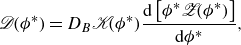 \begin{equation} \mathscr{D}(\phi ^*) = D_B\mathscr{K}(\phi ^*)\frac {{\rm d}\left [\phi ^*\mathscr{Z}(\phi ^*)\right ]}{{\rm d}\phi ^*}, \end{equation}
where $D_B$
is the diffusivity coefficient given by the Stokes–Einstein formula as
$D_B$
is the diffusivity coefficient given by the Stokes–Einstein formula as
 \begin{align} D_B = \frac {K_BT^\ast }{3\pi \mu ^\ast _{bf}d_p^\ast }, \end{align}
and $K_B$
is the Boltzmann constant,
$K_B$
is the Boltzmann constant, $K_B= 1.380649 \times 10^{-23}$
JK−1. The generalised Stokes–Einstein formula (2.3) exhibits a strong dependence of the diffusion coefficient on the local nanoparticle concentration via hydrodynamic and thermodynamic interaction given by the sedimentation coefficient
$K_B= 1.380649 \times 10^{-23}$
JK−1. The generalised Stokes–Einstein formula (2.3) exhibits a strong dependence of the diffusion coefficient on the local nanoparticle concentration via hydrodynamic and thermodynamic interaction given by the sedimentation coefficient $\mathscr{K}(\phi ^*)$
and the compressibility contribution
$\mathscr{K}(\phi ^*)$
and the compressibility contribution $\mathscr{Z}(\phi ^*)$
, respectively. Combining the Carnahan & Starling (Reference Carnahan and Starling1969) equation for the compressibility effect
$\mathscr{Z}(\phi ^*)$
, respectively. Combining the Carnahan & Starling (Reference Carnahan and Starling1969) equation for the compressibility effect $\displaystyle \mathscr{Z}(\phi ^*) = \frac {1+\phi ^*+\phi ^{*2}-\phi ^{*3}}{ (1-\phi ^* )^3}$
and the semi-empirical expression for the sedimentation coefficient
$\displaystyle \mathscr{Z}(\phi ^*) = \frac {1+\phi ^*+\phi ^{*2}-\phi ^{*3}}{ (1-\phi ^* )^3}$
and the semi-empirical expression for the sedimentation coefficient $\displaystyle \mathscr{K}(\phi ^*) = (1-\phi ^* )^{6.55}$
, Russel et al. (Reference Russel, Saville and Schowalter1989) derived the following form for the generalised Stokes–Einstein formula:
$\displaystyle \mathscr{K}(\phi ^*) = (1-\phi ^* )^{6.55}$
, Russel et al. (Reference Russel, Saville and Schowalter1989) derived the following form for the generalised Stokes–Einstein formula:
 \begin{equation} \mathscr{D}^\ast (\phi ^*) = D_B\left (1-\phi ^*\right )^{2.55}\left (1+4\phi ^*+4\phi ^{*2}-4\phi ^{*3}+\phi ^{*4}\right ), \end{equation}
which reduces for low particle concentrations $\phi ^\ast$
to
$\phi ^\ast$
to
 \begin{equation} \mathscr{D}^\ast (\phi ^*) = D_B\left (1+1.45 \phi ^\ast \right ) \end{equation}
previously derived by Batchelor (Reference Batchelor1976). Despite this, in our investigation below, we will use a constant value for the Brownian diffusivity coefficient $\mathscr{D}^\ast (\phi ^*) = D_B$
with the justification given towards the end of § 2.3 and in § 4.4.
$\mathscr{D}^\ast (\phi ^*) = D_B$
with the justification given towards the end of § 2.3 and in § 4.4.
The second slip mechanism is due to the fact that the nanofluid layer is non-isothermal. The temperature gradient induces a flux of nanoparticles, and this phenomenon is known as the thermophoresis or the Soret effect. The Soret or thermal diffusion coefficient in a nanofluid is proportional to the particle concentration $\phi ^\ast$
and is expressed by Whitmore & Meisen (Reference Whitmore and Meisen1977) and Morozov (Reference Morozov2002) as
$\phi ^\ast$
and is expressed by Whitmore & Meisen (Reference Whitmore and Meisen1977) and Morozov (Reference Morozov2002) as
 \begin{equation} D_T = \left (\frac {0.26K^\ast _{bf}}{2K^\ast _{bf}+K^\ast _{np}}\right )\frac {\mu ^\ast _{bf}}{\rho ^\ast _{bf}}\phi ^\ast . \end{equation}
In what follows, we consider the total nanoparticle mass flux as a superposition of the Brownian and Soret diffusion processes via
 \begin{equation} \textbf{j}_p = -\rho ^\ast _{np}\left ( C_BT^\ast \nabla ^\ast \phi ^\ast + C_T\phi ^\ast \frac {\nabla ^\ast T^\ast }{T^\ast }\right ), \end{equation}
where $C_B = D_B/T^\ast$
,
$C_B = D_B/T^\ast$
, $C_T = D_T/\phi ^\ast$
and
$C_T = D_T/\phi ^\ast$
and $\displaystyle \nabla ^\ast = (\partial _{x^\ast }, \partial _{y^\ast },\partial _{z^\ast } )$
with subscripts
$\displaystyle \nabla ^\ast = (\partial _{x^\ast }, \partial _{y^\ast },\partial _{z^\ast } )$
with subscripts ${x^\ast }, {y^\ast },{z^\ast }$
denoting partial differentiation with respect to the corresponding variable. Buzzaccaro et al. (Reference Buzzaccaro, Tripodi, Rusconi, Vigolo and Piazza2008) noted that the expression in the parentheses in (2.6) is valid for relatively large nanoparticles of diameter
${x^\ast }, {y^\ast },{z^\ast }$
denoting partial differentiation with respect to the corresponding variable. Buzzaccaro et al. (Reference Buzzaccaro, Tripodi, Rusconi, Vigolo and Piazza2008) noted that the expression in the parentheses in (2.6) is valid for relatively large nanoparticles of diameter $1$
$1$ $\mu$
m in water. In fact, it was found that the Soret coefficient
$\mu$
m in water. In fact, it was found that the Soret coefficient $C_T$
depends on the nanoparticle size (Braibanti, Vigolo & Piazza Reference Braibanti, Vigolo and Piazza2008; Michaelides Reference Michaelides2015). It is also important to note that the total particle mass flux given by (2.7) ensures a consistently positive distribution of nanoparticle concentration across the nanofluid layer even when subjected to a strong thermophoresis. However, we also note that a use of a constant Soret coefficient in front of the
$C_T$
depends on the nanoparticle size (Braibanti, Vigolo & Piazza Reference Braibanti, Vigolo and Piazza2008; Michaelides Reference Michaelides2015). It is also important to note that the total particle mass flux given by (2.7) ensures a consistently positive distribution of nanoparticle concentration across the nanofluid layer even when subjected to a strong thermophoresis. However, we also note that a use of a constant Soret coefficient in front of the $\nabla ^\ast T^\ast$
term in (2.7) is constrained to a range bounded from above for this coefficient, since beyond this range, spurious unphysical negative values for the particle concentration
$\nabla ^\ast T^\ast$
term in (2.7) is constrained to a range bounded from above for this coefficient, since beyond this range, spurious unphysical negative values for the particle concentration $\phi ^\ast$
emerge. This fact was also emphasised by Dastvareh & Azaiez (Reference Dastvareh and Azaiez2018).
$\phi ^\ast$
emerge. This fact was also emphasised by Dastvareh & Azaiez (Reference Dastvareh and Azaiez2018).
The other five slip mechanisms mentioned by Buongiorno (Reference Buongiorno2006) are inertia, diffusiophoresis, Magnus effect, fluid drainage and gravitational settling. Inertia has a negligible effect due to the homogeneous motion of nanoparticles with the surrounding continuum media. We neglect the diffusiophoresis effect for a one-component nanofluid; however, it may be important when the base fluid is subjected to an additional solute species gradient (Ruckenstein Reference Ruckenstein1981; Anderson Reference Anderson1989; Morozov Reference Morozov2002). The Magnus effect arises due to a force perpendicular to the main flow direction, induced by the relative axial velocity between the nanoparticle and fluid flow. We neglect the Magnus effect as well considering an homogeneous motion of the nanoparticles with the surrounding fluid. The fluid drainage contribution is important for the distance between the wall and particle of the order of nanoparticle diameter and can be neglected for nanoparticles with a small diameter $d^\ast _{p}$
.
$d^\ast _{p}$
.
The relative strength of the particle flux due to gravitational settling (Mason & Weaver Reference Mason and Weaver1924; Shliomis & Smorodin Reference Shliomis and Smorodin2005; Buzzaccaro et al. Reference Buzzaccaro, Tripodi, Rusconi, Vigolo and Piazza2008; Cherepanov & Smorodin Reference Cherepanov and Smorodin2019) versus the flux due to Brownian diffusion may be estimated by the ratio
 \begin{equation} \mathcal{S}_g = \frac {h_0^*(\rho _{np}^*-\rho _{bf}^*)g^*(\pi d_p^{*3}/6)}{K_B T_r^*}. \end{equation}
For nanoparticles of $d_p^*\approx 10\,\text{nm and }\rho ^\ast _{np}\sim 4\,\text{g cm}^{-3}$
in a nanofluid layer of
$d_p^*\approx 10\,\text{nm and }\rho ^\ast _{np}\sim 4\,\text{g cm}^{-3}$
in a nanofluid layer of $0.1$
mm thickness at room temperature, and the terrestrial gravity is
$0.1$
mm thickness at room temperature, and the terrestrial gravity is $\mathcal{S}_g\approx 3.7\times 10^{-4}$
and, therefore, the mass flux induced by gravitational settling may be neglected. However, gravitational settling contributes significantly for nanoparticles with a larger diameter, say of
$\mathcal{S}_g\approx 3.7\times 10^{-4}$
and, therefore, the mass flux induced by gravitational settling may be neglected. However, gravitational settling contributes significantly for nanoparticles with a larger diameter, say of $d_p^*\approx 100$
nm with
$d_p^*\approx 100$
nm with $\mathcal{S}_g\approx 0.37$
. Therefore, in the latter case, the contribution of gravitational settling could not be disregarded, see also Chang & Ruo (Reference Chang and Ruo2022) and their modification for the mass flux, their (2.3). For more details, see also Appendix A.2.
$\mathcal{S}_g\approx 0.37$
. Therefore, in the latter case, the contribution of gravitational settling could not be disregarded, see also Chang & Ruo (Reference Chang and Ruo2022) and their modification for the mass flux, their (2.3). For more details, see also Appendix A.2.
Finally, the heat flux in a nanofluid is given by Fourier’s law of heat conduction,
 \begin{equation} \textbf{j}_T = - K_{nf}^\ast \nabla ^\ast T^\ast . \end{equation}
The Dufour effect is exceedingly weak in liquid mixtures (Cross & Hohenberg Reference Cross and Hohenberg1993; Oron & Nepomnyashchy Reference Oron and Nepomnyashchy2004; Morozov et al. Reference Morozov, Oron and Nepomnyashchy2014) and can be safely neglected in the case at hand. We also note that following Buongiorno (Reference Buongiorno2006), the expression for the heat flux $\textbf{j}_T$
in (2.9) of Chang & Ruo (Reference Chang and Ruo2022) had four more terms, with one of them arising from gravitational settling. All these terms are found to be negligible in our case in comparison with the heat conduction term there, and will be omitted in what follows. A justification for this simplification will be presented in § 2.3 in the context of non-dimensional equations (2.13).
$\textbf{j}_T$
in (2.9) of Chang & Ruo (Reference Chang and Ruo2022) had four more terms, with one of them arising from gravitational settling. All these terms are found to be negligible in our case in comparison with the heat conduction term there, and will be omitted in what follows. A justification for this simplification will be presented in § 2.3 in the context of non-dimensional equations (2.13).
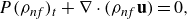
2.3. Governing equations
The set of governing equations comprises the continuity, Navier–Stokes, advection–conduction heat transfer and nanoparticle mass transfer equations (Rohsenow, Hartnett & Cho Reference Rohsenow, Hartnett and Cho1998; Batchelor Reference Batchelor2000; Colinet, Legros & Velarde Reference Colinet, Legros and Velarde2001; Bird et al. Reference Bird, Stewart and Lightfoot2002), respectively
 \begin{align}&\qquad\qquad\qquad (\rho _{nf}^*)_{t^*} + \nabla ^\ast \cdot (\rho _{nf}^*\textbf{u}^*) = 0, \end{align}
 \begin{align}& (\rho _{nf}^*\textbf{u}^*)_{t^*} + \nabla ^\ast \cdot (\rho _{nf}^*\textbf{u}^*\textbf{u}^*) = -\nabla ^\ast p^* + \nabla ^\ast \cdot \boldsymbol{\tau }^* -\rho _{nf}^*g^*\textbf{e}_{z^*}, \end{align}
 \begin{align}&\,\, (\rho ^* c^*)_{nf}(T^*)_{t^*} + (\rho ^* c^*)_{nf} (\textbf{u}^\ast \cdot \nabla ^\ast ) T^\ast = \nabla ^\ast \cdot (K_{nf}^*\nabla ^\ast T^*), \end{align}
 \begin{align}&\,\,\, (\phi ^*)_{t^*} + \nabla ^\ast \cdot (\textbf{u}^*\phi ^*) = \nabla ^\ast \cdot \Big(C_BT^*\nabla ^\ast \phi ^* +C_T\phi ^*\frac {\nabla ^\ast T^*}{T^*}\Big), \end{align}
where $g^*$
is the gravity acceleration,
$g^*$
is the gravity acceleration, $\textbf{e}_{z^*}$
is the unit vector in the
$\textbf{e}_{z^*}$
is the unit vector in the $z^\ast$
direction,
$z^\ast$
direction, ${\textbf u}^* = (u^*,v^*,w^* )$
is the flow field vector and
${\textbf u}^* = (u^*,v^*,w^* )$
is the flow field vector and $\boldsymbol{\tau }^*$
is the viscous part of the stress tensor
$\boldsymbol{\tau }^*$
is the viscous part of the stress tensor $\displaystyle \boldsymbol{\tau }^* =\mu _{nf}^\ast (\nabla ^\ast {\textbf u^*}+ (\nabla ^\ast {\textbf u^*} )^\intercal ) - \Big(\frac {2}{3}\mu _{nf}^\ast - \mathcal{K}^\ast \Big) (\nabla ^\ast \cdot \textbf{u}^\ast ) \textbf{I}$
, where the superscript
$\displaystyle \boldsymbol{\tau }^* =\mu _{nf}^\ast (\nabla ^\ast {\textbf u^*}+ (\nabla ^\ast {\textbf u^*} )^\intercal ) - \Big(\frac {2}{3}\mu _{nf}^\ast - \mathcal{K}^\ast \Big) (\nabla ^\ast \cdot \textbf{u}^\ast ) \textbf{I}$
, where the superscript $^\intercal$
denotes the transpose of the corresponding tensor,
$^\intercal$
denotes the transpose of the corresponding tensor, $\textbf{I}$
is the unity tensor, the subscript
$\textbf{I}$
is the unity tensor, the subscript $t^\ast$
stands for a partial derivative with respect to time
$t^\ast$
stands for a partial derivative with respect to time $t^\ast$
and
$t^\ast$
and $\mathcal{K}^\ast$
is the dilatational viscosity of the fluid. We note that the last term in (2.10b
) represents the buoyancy force which is due to the fluid density varying within the layer with the particle concentration that is in turn coupled to the fluid temperature via the governing equations (2.10).
$\mathcal{K}^\ast$
is the dilatational viscosity of the fluid. We note that the last term in (2.10b
) represents the buoyancy force which is due to the fluid density varying within the layer with the particle concentration that is in turn coupled to the fluid temperature via the governing equations (2.10).
We impose three boundary conditions at the solid–liquid interface $z^*=0$
. At the substrate, the fluid velocity exhibits no-slip and no-penetration, zero total mass flux implying the impermeability of the substrate, and a constant prescribed heat flux
$z^*=0$
. At the substrate, the fluid velocity exhibits no-slip and no-penetration, zero total mass flux implying the impermeability of the substrate, and a constant prescribed heat flux $\mathcal{Q}q^*$
. We note that it is quite natural to prescribe the heat flux at the substrate to better fit experimental settings in the case where the substrate is not made of material with a high thermal conductivity (Rohsenow et al. Reference Rohsenow, Hartnett and Cho1998):
$\mathcal{Q}q^*$
. We note that it is quite natural to prescribe the heat flux at the substrate to better fit experimental settings in the case where the substrate is not made of material with a high thermal conductivity (Rohsenow et al. Reference Rohsenow, Hartnett and Cho1998):
 \begin{equation} z^\ast =0: \quad \textbf{u}^* = 0, \quad -K_{nf}^{*}T^*_{z^\ast } = \mathcal{Q}q^*, \quad C_BT^* \phi ^*_{z^\ast }+C_T\phi ^*\frac {T^*_{z^\ast }}{T^*} = 0. \end{equation}
At the deformable interface $z^* = h^*(x^*,y^*,t^*)$
, we impose the kinematic boundary condition, the continuity of the normal and tangential stresses, the continuity of the heat flux and impermeability for mass transfer, respectively
$z^* = h^*(x^*,y^*,t^*)$
, we impose the kinematic boundary condition, the continuity of the normal and tangential stresses, the continuity of the heat flux and impermeability for mass transfer, respectively
 \begin{align}&\qquad\qquad\qquad\qquad\quad h_{t^*}^*+u^*h_{x^*}^*+v^*h_{y^*}^*=w^*, \end{align}
 \begin{align}& {\textbf{n}}^\ast \cdot \boldsymbol{\mathcal{T}}^*\cdot {\textbf{n}}^\ast = 2\boldsymbol{\mathcal{H}^\ast }\sigma ^\ast, \quad {\textbf{n}}^\ast \cdot \boldsymbol{\mathcal{T}}^*\cdot \textbf{x}^\ast = \textbf{x}^\ast \cdot \nabla ^\ast _s\sigma ^*,\quad {\textbf{n}}^\ast \cdot \boldsymbol{\mathcal{T}}^*\cdot \textbf{y}^\ast = \textbf{y}^\ast \cdot \nabla ^\ast _s\sigma ^*, \end{align}
 \begin{align}&\qquad\qquad\qquad\qquad -K_{nf}^*\nabla ^\ast T^*\cdot {\textbf{n}}^\ast =\widehat {q}(T^*-T_\infty ^*), \end{align}
 \begin{align}&\qquad\qquad\qquad\quad \Big(C_BT^*\nabla ^\ast \phi ^*+C_T\phi ^*\frac {\nabla ^\ast T^*}{T^*}\Big)\cdot {\textbf{n}}^\ast =0, \end{align}
where ${\nabla }^{\ast} _s = (\textbf{I} - {\textbf{n}}^\ast {\textbf{n}}^\ast )\cdot {\nabla }^\ast$
is the surface gradient operator,
${\nabla }^{\ast} _s = (\textbf{I} - {\textbf{n}}^\ast {\textbf{n}}^\ast )\cdot {\nabla }^\ast$
is the surface gradient operator,
 \begin{align} {\textbf{n}}^\ast = \frac {-h_{x^*}^*\textbf{e}_{x^*}-h_{y^*}^*\textbf{e}_{y^*}+\textbf{e}_{z^*}}{\sqrt {1+h_{x^*}^{*2}+h_{y^*}^{*2}}} \end{align}
is the unit vector normal to the interface, $\textbf{e}_{x^\ast }$
and
$\textbf{e}_{x^\ast }$
and $\textbf{e}_{y^\ast }$
are the orthonormal vectors in the
$\textbf{e}_{y^\ast }$
are the orthonormal vectors in the $x^\ast$
and
$x^\ast$
and $y^\ast$
directions, respectively,
$y^\ast$
directions, respectively,
 \begin{align} \textbf{x}^\ast = \frac {\textbf{e}_{x^*}+h_{x^*}^* \textbf{e}_{z^\ast}}{\sqrt {1+h_{x^*}^{*2}}},\quad \textbf{y}^\ast =\frac {\textbf{e}_{y^*}+h_{y^*}^* \textbf{e}_{z^\ast}}{\sqrt {1+h_{y^*}^{*2}}}, \end{align}
are unit vectors tangent to the interface, $\boldsymbol{\mathcal{T}}^*$
is total stress tensor
$\boldsymbol{\mathcal{T}}^*$
is total stress tensor
 \begin{align} \boldsymbol{\mathcal{T}}^* = -p^*\textbf{I} + \mu _{nf}^*\left (\nabla ^\ast {{\textbf{u}}^*}+ \left (\nabla ^\ast {{\textbf{u}}^*}\right )^\intercal \right ) -\left (\frac {2}{3}\mu _{nf}^\ast - {\mathcal{K}}^\ast \right )\left (\nabla ^\ast \cdot {\textbf{u}}^\ast \right ) \textbf{I}, \end{align} $2\boldsymbol{\mathcal{H}}^*$
is the mean curvature of the interface
$2\boldsymbol{\mathcal{H}}^*$
is the mean curvature of the interface
 \begin{align} 2\boldsymbol{\mathcal{H}}^* = -\nabla ^\ast _s\cdot {\textbf{n}}^\ast, \end{align}
and $\widehat {q}$
is the rate of heat transfer from the liquid phase to the gas phase by convection according to Newton’s law of cooling. We note that Stokes’ hypothesis (Buresti Reference Buresti2015) of a zero value of the dilatational viscosity
$\widehat {q}$
is the rate of heat transfer from the liquid phase to the gas phase by convection according to Newton’s law of cooling. We note that Stokes’ hypothesis (Buresti Reference Buresti2015) of a zero value of the dilatational viscosity $\mathcal{K}^\ast$
will be used in what follows. This implies that the absolute value of
$\mathcal{K}^\ast$
will be used in what follows. This implies that the absolute value of $\mathcal{K}^\ast \nabla ^\ast \cdot {\textbf{u}}^\ast$
is negligible compared with the thermodynamic pressure
$\mathcal{K}^\ast \nabla ^\ast \cdot {\textbf{u}}^\ast$
is negligible compared with the thermodynamic pressure $p^\ast$
, i.e.
$p^\ast$
, i.e. $|\mathcal{K}^\ast \nabla ^\ast \cdot {\textbf{u}}^\ast |\ll p^\ast$
.
$|\mathcal{K}^\ast \nabla ^\ast \cdot {\textbf{u}}^\ast |\ll p^\ast$
.
To obtain the closure of the problem, one more condition needs to be added. The average solute concentration $\Phi ^*$
is determined via
$\Phi ^*$
is determined via
 \begin{equation} \Phi ^*=\frac {1}{I({{\mathcal{D}}^\ast })h_0^\ast }\int _0^{h^\ast } \left (\int \int _{{\mathcal{D}}^\ast }{\phi ^\ast (x^\ast, y^\ast, z^*)}{\rm d}x^*{\rm d}y^\ast \right ){\rm d}z^\ast, \end{equation}
where ${\mathcal{D}}^*$
is a projection of the flow domain onto the
${\mathcal{D}}^*$
is a projection of the flow domain onto the $x^\ast {-}y^\ast$
plane and
$x^\ast {-}y^\ast$
plane and $I({{\mathcal{D}}^*})$
is the area of this projection. A needed closure of the problem is obtained by imposing a constraint that the value
$I({{\mathcal{D}}^*})$
is the area of this projection. A needed closure of the problem is obtained by imposing a constraint that the value $\Phi ^*$
is prescribed and fixed. We note that the condition of the constant nanoparticle averaged bulk concentration
$\Phi ^*$
is prescribed and fixed. We note that the condition of the constant nanoparticle averaged bulk concentration $\Phi ^*$
is appropriate for the case of the quiescent base state. However, in the presence of the base state flow, the conservation of the nanoparticle mass flux should be employed (Krishnan, Beimfohr & Leighton Reference Krishnan, Beimfohr and Leighton1996; Frank et al. Reference Frank, Anderson, Weeks and Morris2003; Ramachandran & Leighton Reference Ramachandran and Leighton2008; Morris Reference Morris2020).
$\Phi ^*$
is appropriate for the case of the quiescent base state. However, in the presence of the base state flow, the conservation of the nanoparticle mass flux should be employed (Krishnan, Beimfohr & Leighton Reference Krishnan, Beimfohr and Leighton1996; Frank et al. Reference Frank, Anderson, Weeks and Morris2003; Ramachandran & Leighton Reference Ramachandran and Leighton2008; Morris Reference Morris2020).
To obtain dimensionless formulation of the problem, we introduce the following normalisation:
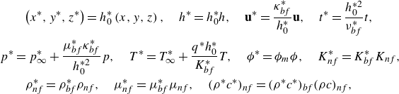 \begin{align} & \qquad \left (x^*,y^*,z^* \right )=h_0^\ast \left (x,y,z\right ),\quad h^{\ast} = h_{0}^{\ast}h, \quad {{\textbf{u}}^*}=\frac {\kappa ^\ast _{bf}}{h_0^\ast } {\textbf{u}}, \quad t^\ast=\frac{h_0^{\ast2}}{\nu^\ast_{bf}} t,\nonumber \\ & \quad p^*=p^\ast _\infty +\frac {\mu ^\ast _{bf}\kappa ^\ast _{bf}}{h_0^{*2}} p, \quad T^*=T^\ast _\infty +\frac {q^\ast h_0^\ast }{K^\ast _{bf}}T,\quad \phi ^* = \phi _m \phi, \quad K^\ast _{nf}=K^\ast _{bf}K_{nf}, \quad \nonumber \\&\qquad\quad \rho _{nf}^* = \rho ^\ast _{bf}\rho _{nf}, \quad \mu _{nf}^*=\mu ^\ast _{bf} \mu _{nf},\quad (\rho ^\ast c^\ast )_{nf} =(\rho ^\ast c^\ast ) _{bf} (\rho c)_{nf}, \end{align}
so the variables with no asterisk decoration are dimensionless.
A set of non-dimensional governing equations and boundary conditions based on this scaling reads
 \begin{align}&\qquad\qquad\quad P(\rho _{nf})_t+\nabla \cdot (\rho _{nf}\textbf{u}) = 0, \end{align}
 \begin{align}& (\rho _{nf}\textbf{u})_t + P^{-1}\nabla \cdot (\rho _{nf}\textbf{u}\textbf{u}) = -\nabla p +\nabla \cdot \boldsymbol{\tau } - \rho _{nf} G {\textbf{e}}_z, \end{align}
 \begin{align}&\qquad\quad (\rho c)_{nf}\left [PT_t + (\textbf{u}\cdot \nabla )T\right ] = \nabla \cdot ( K_{nf}\nabla T), \end{align}
 \begin{align}&\quad\,\, PL^{-1}\phi _t + L^{-1}\nabla \cdot (\textbf{u}\phi ) = \nabla ^2\phi + \nabla \cdot (\eta \phi \nabla T), \end{align}
where $\displaystyle \nabla \equiv ({\partial }/{\partial x}, {\partial }/{\partial y},{\partial }/{\partial z} )$
, and
$\displaystyle \nabla \equiv ({\partial }/{\partial x}, {\partial }/{\partial y},{\partial }/{\partial z} )$
, and $\displaystyle \boldsymbol{\tau } =\mu _{nf} [\nabla {\textbf{u}}+ \nabla {\textbf{u}}^\intercal - {2}/{3} (\nabla \cdot \textbf{u} ) \textbf{I} ]$
is the viscous part of the dimensionless stress tensor.
$\displaystyle \boldsymbol{\tau } =\mu _{nf} [\nabla {\textbf{u}}+ \nabla {\textbf{u}}^\intercal - {2}/{3} (\nabla \cdot \textbf{u} ) \textbf{I} ]$
is the viscous part of the dimensionless stress tensor.
The energy conservation equation (2.9) of Chang & Ruo (Reference Chang and Ruo2022) is written following Buongiorno (Reference Buongiorno2006) in terms of our dimensionless variables as
 \begin{align} (\rho c)_{nf}\left [PT_t + (\textbf{u}\cdot \nabla )T\right ] &= \nabla \cdot ( K_{nf}\nabla T) + \mathscr{K}_1 \nabla \phi \cdot \nabla T + \mathscr{K}_2T\nabla \phi \cdot \nabla T + \mathscr{K}_3\phi \nabla T\cdot \nabla T \nonumber\\&\quad + \mathscr{K}_4\phi \nabla T, \end{align}
where
 \begin{align} &\mathscr{K}_1 = \frac {(\rho c)_{np}^*C_BT_{\infty }^*\phi _m}{(\rho c)_{bf}^*\kappa _{bf}^*}\sim 10^{-4},\quad \mathscr{K}_2 = \frac {(\rho c)_{np}^*C_B\Delta T^*\phi _m}{(\rho c)_{bf}^*\kappa _{bf}^*}\sim 10^{-7},\nonumber\\ &\,\,\mathscr{K}_3 = \frac {(\rho c)_{np}^*C_T\phi _m\Delta T^*}{(\rho c)_{bf}^*\kappa _{bf}^*T_{\infty }^*}\sim 10^{-5},\quad \mathscr{K}_4 = \frac {(\rho c)_{np}^*h_0^*\mathcal{S}_g\phi _m}{(\rho c)_{bf}^*\kappa _{bf}^*} \sim 10^{-5}. \end{align}
It is noted that the $\mathscr{K}_4$
term is related to gravitational settling. Based on the typical values of the parameters in (2.15), in what follows, we neglect the contribution of the nanoparticle mass flux to heat transfer for
$\mathscr{K}_4$
term is related to gravitational settling. Based on the typical values of the parameters in (2.15), in what follows, we neglect the contribution of the nanoparticle mass flux to heat transfer for $h_0^*\approx 10^{-6}$
m. For much thicker layers and bigger nanoparticles, the contribution of gravitational settling needs to be included in (2.13c
).
$h_0^*\approx 10^{-6}$
m. For much thicker layers and bigger nanoparticles, the contribution of gravitational settling needs to be included in (2.13c
).
The non-dimensional boundary conditions at $z=0$
are
$z=0$
are
 \begin{equation} \textbf{u} = 0,\quad K_{nf} T_z = -\mathcal{Q},\quad \phi _z + \eta \phi T_z =0. \end{equation}
The non-dimensional boundary conditions at $z = h$
are
$z = h$
are
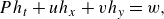 \begin{align}&\qquad\qquad\qquad\qquad Ph_t+uh_x+vh_y=w, \end{align}
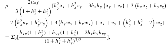 \begin{align}& -p - \frac {2\mu _{nf}}{3\left (1+h_{x}^{2} + h_{y}^{2}\right ) }\Big[h_y^2 u_x + h_x^2 v_y - 3 h_x h_y \left (u_y + v_x \right ) + 3 \left (h_x u_z + h_y v_z \right ) \nonumber\\&\quad- 2 \left (h_x^2 u_x + h_y^2 v_y \right ) + 3 \left (h_y w_y + h_x w_x \right ) + u_x+ v_y + \left (h_y^2 + h_x^2 - 2\right ) w_z \Big] \nonumber\\&\quad = \Sigma _0\Big[\frac {h_{xx}(1+h_{y}^{2})+h_{yy}(1+h_{x}^{2})-2h_{x}h_{y}h_{xy}}{(1+h_{x}^{2}+h_{y}^{2})^{3/2}}\Big], \end{align}
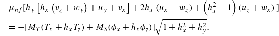 \begin{align}& -\mu _{nf} \Big [h_y \left [h_x \left (v_z+w_y\right )+u_y+v_x\right ]+2 h_x \left (u_x-w_z\right )+\left (h_{x}^2-1\right ) \left (u_z + w_x \right ) \Big ] \nonumber\\&\quad = -\Big [M_T(T_x + h_x T_z) + M_S(\phi _x + h_x\phi _z)\Big ]\sqrt {1+h_{x}^{2} + h_{y}^{2} }, \end{align}
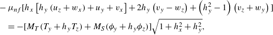 \begin{align}& -\mu _{nf} \Big[h_x \left [h_{y} \left (u_z+w_x\right )+ u_y+v_x \right ] + 2 h_y \left (v_y - w_z \right ) +\left (h_y^2-1\right ) \left (v_z + w_y \right )\Big] \nonumber\\&\quad = -\Big [M_T(T_y + h_y T_z) + M_S(\phi _y + h_y\phi _z)\Big ]\sqrt {1+h_x^2+h_y^2}, \end{align}
 \begin{align}&\qquad\qquad\quad K_{nf}\nabla T\cdot \textbf{n}+BT=0,\quad \left (\nabla \phi + \eta \phi \nabla T\right )\cdot \textbf{n}= 0, \end{align}
where $P,\,G,\, L,\, B,\, M_T,\, M_S,\,\Sigma _0,\,\eta \ \text{and}\ \mathcal{Q}$
are respectively the Prandtl, the modified Galileo, Lewis, Biot, thermal Marangoni, solutal Marangoni, and dimensionless surface tension numbers, the Soret coefficient and the direction of the applied heat flux,
$P,\,G,\, L,\, B,\, M_T,\, M_S,\,\Sigma _0,\,\eta \ \text{and}\ \mathcal{Q}$
are respectively the Prandtl, the modified Galileo, Lewis, Biot, thermal Marangoni, solutal Marangoni, and dimensionless surface tension numbers, the Soret coefficient and the direction of the applied heat flux,
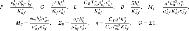 \begin{align} &P=\frac {\nu ^\ast _{bf} \rho ^\ast _{bf} c_{bf}^\ast }{K^\ast _{bf}}, \!\quad G=\frac {g^\ast h_0^{*3}}{\nu ^\ast _{bf}\kappa ^\ast _{bf}}, \!\quad L=\frac {C_B T^\ast _\infty \rho ^\ast _{bf} c_{bf}^\ast }{K^\ast _{bf}}, \!\quad B=\frac {\widehat {q}h_0^\ast }{K^\ast _{bf}},\!\quad M_T = \frac {q^\ast h_0^{*2} \sigma ^\ast_{T^\ast}}{\mu ^\ast _{bf}K^\ast _{bf} \kappa ^\ast _{bf}},\nonumber \\&\qquad\quad M_S = \frac {\phi _mh_0^\ast \sigma^\ast _{\phi ^\ast }}{\mu ^\ast _{bf}\kappa ^\ast _{bf}}, \quad \Sigma _0 = \frac {\sigma ^\ast _rh_0^\ast }{\mu ^\ast _{bf}\kappa ^\ast _{bf}},\quad \eta = \frac {C_T q^\ast h_0^\ast }{C_BT_\infty ^{\ast 2} K^\ast _{bf}}, \quad \mathcal{Q} = \pm 1. \end{align}
In addition, the dimensionless form of the thermophysical properties appearing in the set of equations (2.13) and (2.16) is
 \begin{align} &\rho _{nf}(\phi ) =(1-\phi \phi _m)+\phi \phi _m\rho _{np},\quad (\rho c)_{nf}(\phi ) = (1-\phi \phi _m)+ \phi \phi _m(\rho c)_{np},\nonumber\\&\qquad\qquad\qquad K_{nf}(\phi ) = 1 + a \phi \phi _m,\quad \mu _{nf}(\phi ) = \left (1-\phi \right )^{-2}. \end{align}
As already mentioned above, in what follows, we assume a constant, particle-concentration independent mass diffusivity. We now wish to explain why the use of a constant diffusivity instead of a particle concentration-dependent diffusivity should not introduce a significant impact on the results. In fact, this is not surprising if the following list of concentration-dependent dimensionless thermophysical properties of the fluid based on (2.18) is written out for a low $\phi$
:
$\phi$
:
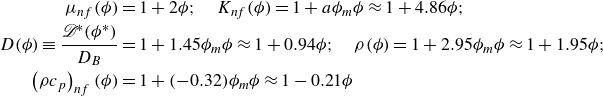 \begin{align} \mu _{nf} (\phi )&=1+2 \phi ; \quad K_{nf} (\phi )=1+a \phi _m \phi \approx 1+4.86 \phi ; \nonumber \\ D(\phi ) \equiv \frac {\mathscr{D}^\ast (\phi ^\ast )}{D_B}&= 1+ 1.45 \phi _m \phi \approx 1+0.94 \phi ; \quad \rho (\phi )= 1+ 2.95 \phi _m \phi \approx 1+ 1.95\phi ;\nonumber \\ \left (\rho c_p \right )_{nf}(\phi )&=1+(-0.32)\phi _m\phi \approx 1-0.21\phi \end{align}
for alumina particles Al $_2$
O
$_2$
O $_3$
in water with
$_3$
in water with $a=7.47$
and
$a=7.47$
and $\phi _m=0.65$
. It is clear that the heat capacity of the nanofluid varies very weakly with
$\phi _m=0.65$
. It is clear that the heat capacity of the nanofluid varies very weakly with $\phi$
, see (2.19), and its dependence on
$\phi$
, see (2.19), and its dependence on $\phi$
may in principle be safely neglected. We also find based on our results (not shown) that using a constant viscosity instead of a concentration-dependent one leads to a negligible deviation, within a few percent, from the results obtained when the varying viscosity
$\phi$
may in principle be safely neglected. We also find based on our results (not shown) that using a constant viscosity instead of a concentration-dependent one leads to a negligible deviation, within a few percent, from the results obtained when the varying viscosity $\mu _{nf}$
is used. Since the variation of the mass diffusivity
$\mu _{nf}$
is used. Since the variation of the mass diffusivity $D(\phi )$
with
$D(\phi )$
with $\phi$
is even weaker than that of the viscosity, as seen in (2.19), being both dissipative effects, it would be logical to assume a constant value for the diffusivity
$\phi$
is even weaker than that of the viscosity, as seen in (2.19), being both dissipative effects, it would be logical to assume a constant value for the diffusivity $D(\phi ) \approx D_B$
, especially because the use of a varying diffusivity prevents from obtaining the base state in the analytical form and would require its fully numerical evaluation with all ensuing consequences and costly computational effort. However, we will return to this issue in § 4.4, where we show that using a constant Brownian diffusion coefficient instead of a particle concentration-dependent one produces a negligible difference in the results, even for small values of
$D(\phi ) \approx D_B$
, especially because the use of a varying diffusivity prevents from obtaining the base state in the analytical form and would require its fully numerical evaluation with all ensuing consequences and costly computational effort. However, we will return to this issue in § 4.4, where we show that using a constant Brownian diffusion coefficient instead of a particle concentration-dependent one produces a negligible difference in the results, even for small values of $a$
.
$a$
.
Recently, Chang & Ruo (Reference Chang and Ruo2022) investigated the Rayleigh–Bénard instability in a nanofluid and considered, among other effects, the presence of density stratification due to both thermal and solutal contributions. To evaluate their relative importance, we introduce the ratio between the thermal Rayleigh number $Ra$
and the solutal Rayleigh number
$Ra$
and the solutal Rayleigh number $Rn$
defined there,
$Rn$
defined there, $\displaystyle R \equiv Ra/Rn= \beta _T^*\Delta T^*/((\rho _{np}-1) \Phi )$
in our notation with
$\displaystyle R \equiv Ra/Rn= \beta _T^*\Delta T^*/((\rho _{np}-1) \Phi )$
in our notation with $\beta _T^*$
being the thermal expansion coefficient. For water as a base fluid,
$\beta _T^*$
being the thermal expansion coefficient. For water as a base fluid, $\beta _T^*\approx 2\times 10^{-4}$
K
$\beta _T^*\approx 2\times 10^{-4}$
K $^{-1}$
(Chang & Ruo Reference Chang and Ruo2022). In the case of the temperature difference between
$^{-1}$
(Chang & Ruo Reference Chang and Ruo2022). In the case of the temperature difference between $1$
K and
$1$
K and $10$
K and the average particle concentration
$10$
K and the average particle concentration $\Phi =0.01$
, we see that
$\Phi =0.01$
, we see that $R$
varies between
$R$
varies between $0.0067$
and
$0.0067$
and $0.067$
, that is,
$0.067$
, that is, $R \ll 1$
, with both bounds decreasing with an increase in
$R \ll 1$
, with both bounds decreasing with an increase in $\Phi$
. We thus neglect the temperature-induced buoyancy effect and consider the buoyancy related to the solutal stratification effect only. We also comment that for a dilute nanosuspension
$\Phi$
. We thus neglect the temperature-induced buoyancy effect and consider the buoyancy related to the solutal stratification effect only. We also comment that for a dilute nanosuspension $\Phi \ll 1$
,
$\Phi \ll 1$
, $R$
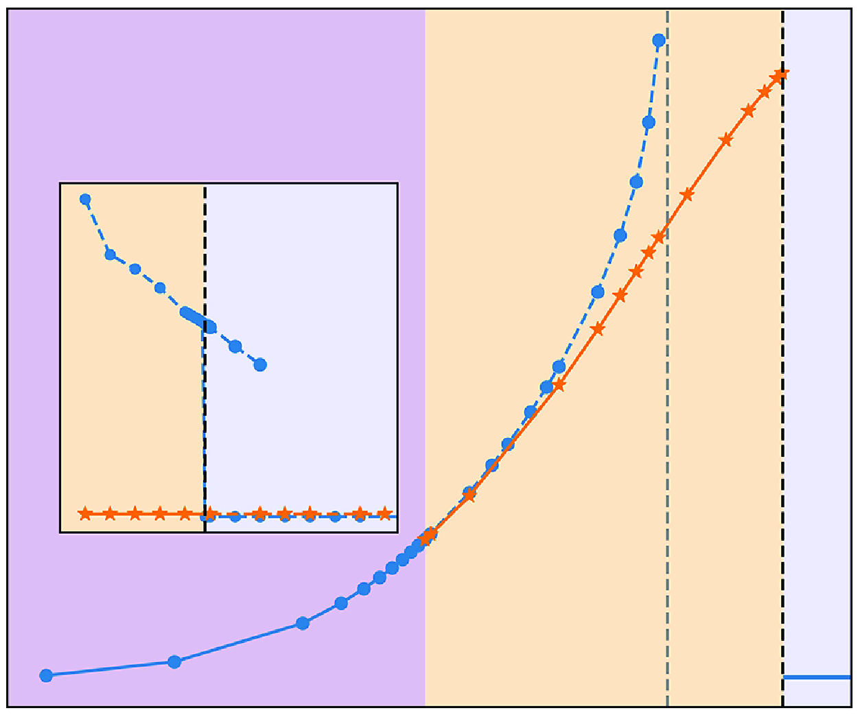
may be of order one, so both effects would have been of the same importance and would have been included in the analysis. In the limiting case of no solute, only the thermal buoyancy term would have remained. Furthermore, in the least favourable case, where in the base state, the concentration in the particle-depleted subdomain is approximately a fifth of the average particle concentration, see figures 2 and 3, the upper bound for the local Rayleigh number ratio
$R$
may be of order one, so both effects would have been of the same importance and would have been included in the analysis. In the limiting case of no solute, only the thermal buoyancy term would have remained. Furthermore, in the least favourable case, where in the base state, the concentration in the particle-depleted subdomain is approximately a fifth of the average particle concentration, see figures 2 and 3, the upper bound for the local Rayleigh number ratio $R = Ra/Rn \approx 0.32$
. For thin layers
$R = Ra/Rn \approx 0.32$
. For thin layers $10^{-6}\,\text{m}\leqslant h_0^*\leqslant 10^{-4}\,\text{m}$
, the relative importance between the two thermal instabilities, namely, thermal Rayleigh
$10^{-6}\,\text{m}\leqslant h_0^*\leqslant 10^{-4}\,\text{m}$
, the relative importance between the two thermal instabilities, namely, thermal Rayleigh $Ra$
and thermal Marangoni
$Ra$
and thermal Marangoni $M_T$
, is given by the dynamic Bond number
$M_T$
, is given by the dynamic Bond number $B_d=Ra/M_T$
. The comparison between the thermal Rayleigh number
$B_d=Ra/M_T$
. The comparison between the thermal Rayleigh number $Ra$
and the thermal Marangoni number
$Ra$
and the thermal Marangoni number $M_T$
shows that for thin layers, their ratio is much lower than
$M_T$
shows that for thin layers, their ratio is much lower than $1$
. More specifically,
$1$
. More specifically,
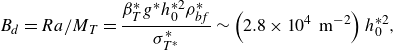 \begin{align} B_d = Ra/M_T = \frac {\beta _T^* g^*h_0^{*2}\rho _{bf}^* }{\sigma _{T^*}^*}\sim \left (2.8\times 10^{4}\,\textrm { m}^{-2}\right ) h_0^{*2}, \end{align}
in the case of an alumina particle suspension in water; therefore, for the layer thickness of $h_0^{*}\approx 10^{-4}$
m, the dynamic Bond number
$h_0^{*}\approx 10^{-4}$
m, the dynamic Bond number $B_d = 2.8\times 10^{-4}$
. Hence, the thermal buoyancy is negligible as compared with the Marangoni effect, and in our case, it may be safely omitted.
$B_d = 2.8\times 10^{-4}$
. Hence, the thermal buoyancy is negligible as compared with the Marangoni effect, and in our case, it may be safely omitted.
We note in passing that the physical problem at hand is isotropic in the $x{-}y$
plane, and therefore, (2.13) and (2.16) possess the symmetry
$x{-}y$
plane, and therefore, (2.13) and (2.16) possess the symmetry $x \leftrightarrow y$
,
$x \leftrightarrow y$
, $u \leftrightarrow v$
and they are written in a way so the symmetry is apparent.
$u \leftrightarrow v$
and they are written in a way so the symmetry is apparent.
2.4. Base state
We now look for a quiescent ( ${\textbf u}= \textbf{u}_0=\textbf{0}$
) steady base state of the system with the flat interface
${\textbf u}= \textbf{u}_0=\textbf{0}$
) steady base state of the system with the flat interface $h=1$
and with the temperature and concentration fields depending solely on
$h=1$
and with the temperature and concentration fields depending solely on $z$
,
$z$
, $T=T_0(z),\, \phi =\phi _0(z)$
, of the problem given by (2.13)–(2.16). It is determined by
$T=T_0(z),\, \phi =\phi _0(z)$
, of the problem given by (2.13)–(2.16). It is determined by
 \begin{align}&\qquad\qquad\qquad\qquad p_{0,z}= - G -G \phi _m \left (\rho _{np}-1\right ) \phi _0, \end{align}
 \begin{align}&\qquad\qquad\qquad\qquad\quad \left [(1+a \phi _m \phi _0)T_{0,z}\right ]_z =0, \end{align}
 \begin{align}&\qquad\qquad\qquad\qquad\quad \left (\phi _{0,z} + \eta \phi _0 T_{0,z}\right )_z=0, \end{align}
 \begin{align}&\qquad\quad z=0: \quad \left (1+a\phi _m\phi _0\right )T_{0,z} = -\mathcal{Q},\quad \phi _{0,z} + \eta \phi _0 T_{0,z} =0, \end{align}
 \begin{align}& z=1: \quad p_0 =0, \quad (1+a \phi _m \phi _0)T_{0,z} +B T_0=0, \quad \phi _{0,z} + \eta \phi _0 T_{0,z}=0. \end{align}
Finally, following (2.11j ),
 \begin{equation} \int _0^1{\phi _0(z)\,{\rm d}z} = \Phi \end{equation}
for a fixed specified positive value $\Phi$
.
$\Phi$
.
The solution of the problem equations (2.21)–(2.22) for the pressure, temperature and concentration components is found to be (details can be found in Appendix A.1)
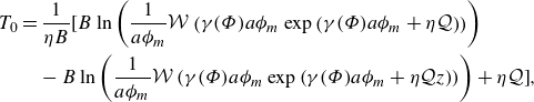 \begin{align}&\qquad\qquad T_0 =\frac {1}{\eta B}\Big [B \ln \left (\frac {1}{a\phi _m}\mathcal{W}\left (\gamma (\Phi ) a\phi _m \exp {\left (\gamma (\Phi ) a\phi _m+\eta \mathcal{Q}\right )}\right )\right )\notag\\&\qquad\qquad\qquad -B \ln \left (\frac {1}{a\phi _m}\mathcal{W}\left (\gamma (\Phi ) a\phi _m \exp {\left (\gamma (\Phi ) a\phi _m+\eta \mathcal{Q} z\right )}\right )\right )+\eta \mathcal{Q}\Big], \end{align}
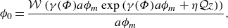 \begin{align}&\qquad\qquad\qquad\qquad \phi _0 =\frac {\mathcal{W}\left (\gamma (\Phi ) a\phi _m \exp {\left (\gamma (\Phi ) a\phi _m+\eta \mathcal{Q} z\right )}\right )}{a\phi _m}, \end{align}
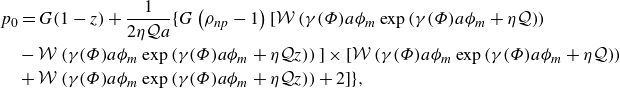 \begin{align}& p_0 = G (1-z) + \frac {1}{2 \eta \mathcal{Q} a}\Big \{G \left (\rho _{np}-1\right ) \Big [\mathcal{W}\left (\gamma (\Phi ) a\phi _m \exp {\left (\gamma (\Phi ) a\phi _m+\eta \mathcal{Q}\right )}\right )\notag\\&\quad -\mathcal{W}\left (\gamma (\Phi ) a\phi _m \exp {\left (\gamma (\Phi ) a\phi _m+\eta \mathcal{Q} z\right )}\right )\Big ]\times \Big [\mathcal{W}\left (\gamma (\Phi ) a\phi _m \exp {\left (\gamma (\Phi ) a\phi _m+\eta \mathcal{Q}\right )}\right )\notag\\&\quad +\mathcal{W}\left (\gamma (\Phi ) a\phi _m \exp {\left (\gamma (\Phi ) a\phi _m+\eta \mathcal{Q} z\right )}\right )+2\Big ]\Big \}, \end{align}
where ${\mathcal{W}}(z)$
is the principal (increasing) branch of the Lambert W function (Corless et al. Reference Corless, Gonnet, Hare, Jeffrey and Knuth1996; Vallis, Parker & Tobias Reference Vallis, Parker and Tobias2019) defined via
${\mathcal{W}}(z)$
is the principal (increasing) branch of the Lambert W function (Corless et al. Reference Corless, Gonnet, Hare, Jeffrey and Knuth1996; Vallis, Parker & Tobias Reference Vallis, Parker and Tobias2019) defined via
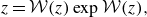 \begin{equation} z={\mathcal{W}}(z) \exp {\mathcal{W}}(z), \end{equation}
and $\gamma (\Phi )$
is determined by substitution of
$\gamma (\Phi )$
is determined by substitution of $\phi _0(z)$
from (2.24b
) into (2.23) to satisfy the conservation of the total volume of nanoparticles. In fact, the value of
$\phi _0(z)$
from (2.24b
) into (2.23) to satisfy the conservation of the total volume of nanoparticles. In fact, the value of $\gamma (\Phi )$
is a solution of (A14) which is solved numerically. We emphasise that the constant
$\gamma (\Phi )$
is a solution of (A14) which is solved numerically. We emphasise that the constant $\gamma (\Phi )$
depends on four more parameters, namely,
$\gamma (\Phi )$
depends on four more parameters, namely, $\phi _m, \eta, \mathcal{Q}$
and
$\phi _m, \eta, \mathcal{Q}$
and $a$
, and the used notation of
$a$
, and the used notation of $\gamma (\Phi )$
is intended only to remind the reader about the source of its appearance. We note that the secondary (decreasing) branch of the Lambert W function yields negative values of
$\gamma (\Phi )$
is intended only to remind the reader about the source of its appearance. We note that the secondary (decreasing) branch of the Lambert W function yields negative values of $\phi_0$
and is therefore irrelevant.
$\phi_0$
and is therefore irrelevant.
Figure 2 presents several examples of the base state in terms of the particle concentration $\phi _0(z)$
(panel a) and temperature
$\phi _0(z)$
(panel a) and temperature $T_0(z)$
(panel b) in the case of cooling at the substrate for various values of the average particle concentration
$T_0(z)$
(panel b) in the case of cooling at the substrate for various values of the average particle concentration $\Phi$
and the temperature drop across the layer in the base state with
$\Phi$
and the temperature drop across the layer in the base state with $\Delta T^*$
determined via
$\Delta T^*$
determined via
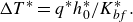 \begin{equation} \Delta T^* = q^\ast h_0^\ast /K^\ast _{bf}. \end{equation}
Furthermore, we observe that the concentration profile shows an opposite variation with height $z$
to that of the temperature profile, owing to the positive value of the Soret coefficient. This leads to the formation of stable stratification in the nanofluid layer. The temperature profile
$z$
to that of the temperature profile, owing to the positive value of the Soret coefficient. This leads to the formation of stable stratification in the nanofluid layer. The temperature profile $T_0(z)$
exhibits a monotonic, almost linear variation with
$T_0(z)$
exhibits a monotonic, almost linear variation with $z$
with a maximal temperature attained at the free surface
$z$
with a maximal temperature attained at the free surface $z=1$
; therefore, the values of the temperature in the bulk are below
$z=1$
; therefore, the values of the temperature in the bulk are below $T_\infty ^*$
, and the difference
$T_\infty ^*$
, and the difference $T_0(z)-T_0(z=1)$
presented in figure 2(b) is negative. We note that the nanoparticle concentration
$T_0(z)-T_0(z=1)$
presented in figure 2(b) is negative. We note that the nanoparticle concentration $\phi _0(z)$
variation with height
$\phi _0(z)$
variation with height $z$
exhibits a nonlinear variation for larger values of the temperature difference
$z$
exhibits a nonlinear variation for larger values of the temperature difference $\Delta T^*$
.
$\Delta T^*$
.
Similarly, we illustrate the base-state profiles of the nanoparticle concentration and temperature for the case of heating at the substrate in figure 3. In contrast with the case of cooling at the substrate, the steady-state profile for the nanoparticle concentration with heating at the substrate depicts an increasing with height $z$
profile of the particle concentration which achieves a maximum at the interface promoted by the Soret effect. Such a profile of the particle concentration represents an unstable density stratification and is prone to a kind of buoyancy instability, which is also similar in spirit to the Rayleigh–Taylor instability and is described in what follows. Opposite to the case of cooling at the substrate, presented in figure 2(b), in the case of heating at the substrate, the temperature increases with height
$z$
profile of the particle concentration which achieves a maximum at the interface promoted by the Soret effect. Such a profile of the particle concentration represents an unstable density stratification and is prone to a kind of buoyancy instability, which is also similar in spirit to the Rayleigh–Taylor instability and is described in what follows. Opposite to the case of cooling at the substrate, presented in figure 2(b), in the case of heating at the substrate, the temperature increases with height $z$
, as presented in figure 3(b).
$z$
, as presented in figure 3(b).
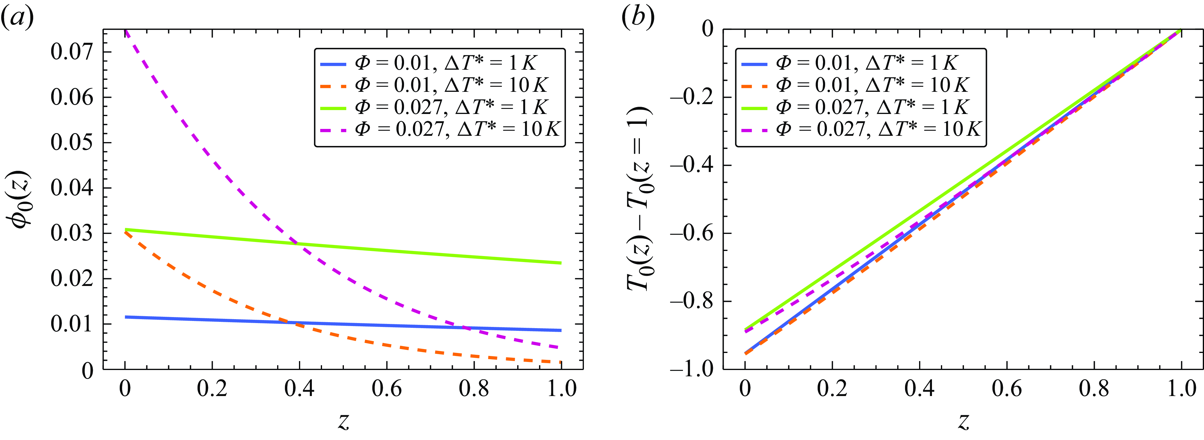
Figure 2. Variation of the quiescent base-state (a) concentration $\phi _0(z)$
and (b) temperature presented as
$\phi _0(z)$
and (b) temperature presented as $T_0(z)-T_0(z=1)$
with height
$T_0(z)-T_0(z=1)$
with height $z$
, for the case of cooling at the substrate
$z$
, for the case of cooling at the substrate $\mathcal{Q}=-1$
, and different values of the averaged bulk concentration
$\mathcal{Q}=-1$
, and different values of the averaged bulk concentration $\Phi$
and temperature difference
$\Phi$
and temperature difference $\Delta T^*$
with
$\Delta T^*$
with $B=0.01,\,\eta =0.31$
and
$B=0.01,\,\eta =0.31$
and $a=7.47$
.
$a=7.47$
.
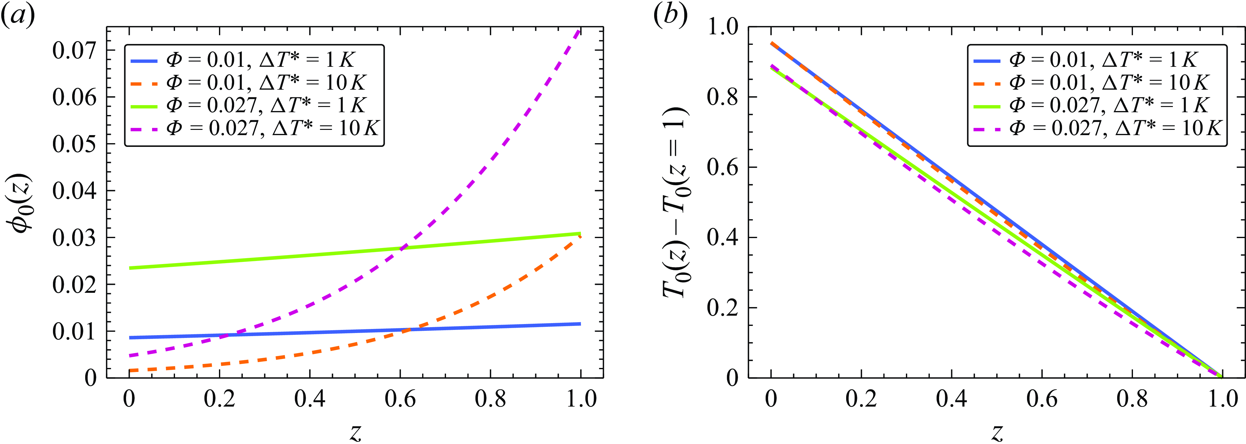
Figure 3. Variation of the quiescent base-state (a) concentration $\phi _0(z)$
and (b) temperature presented as
$\phi _0(z)$
and (b) temperature presented as $T_0(z)-T_0(z=1)$
with height
$T_0(z)-T_0(z=1)$
with height $z$
, for the case of heating at the substrate
$z$
, for the case of heating at the substrate $\mathcal{Q}=1$
, and different values of the averaged bulk concentration
$\mathcal{Q}=1$
, and different values of the averaged bulk concentration $\Phi$
and temperature difference
$\Phi$
and temperature difference $\Delta T^*$
with
$\Delta T^*$
with $B=0.01,\,\eta =0.31$
and
$B=0.01,\,\eta =0.31$
and $a=7.47$
.
$a=7.47$
.
3. Linear stability analysis
We now investigate the linear stability of the base state given by (2.24) with ${\textbf{u}}_0=0$
and
${\textbf{u}}_0=0$
and $h_0=1$
. To do this, the fields of the dependent variables are linearised around the base state in the form
$h_0=1$
. To do this, the fields of the dependent variables are linearised around the base state in the form
 \begin{equation} {\textbf u} = {\textbf{u}}_0+\bar {{\textbf u}}= \bar {\textbf u}, \quad p=p_0+\bar {p}, \quad T=T_0+\bar {T}, \quad \phi =\phi _0+\bar {\phi }, \quad h = h_0 + \bar {\zeta }, \end{equation}
where the values with an overbar represent the disturbances of the corresponding fields. Furthermore, we linearise the thermophysical properties around the dimensionless base state concentration $\phi _0$
, i.e.
$\phi _0$
, i.e.
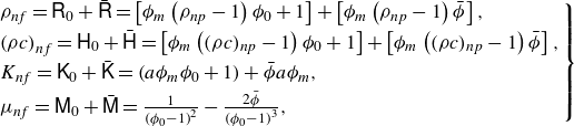 \begin{align} \left . \begin{array}{ll} \rho _{nf} = \textsf{R}_0 + \bar {\textsf{R}} = \left [\phi _m \left (\rho _{np}-1\right ) \phi _0 + 1 \right ]+ \left [\phi _m \left (\rho _{np}-1\right ) \bar {\phi }\right ],\\[3pt] \left (\rho c\right )_{nf} = \textsf{H}_0 + \bar {\textsf{H}} = \left [\phi _m \left ((\rho c) _{np}-1\right ) \phi _0 + 1 \right ]+ \left [\phi _m \left ((\rho c) _{np}-1\right ) \bar {\phi }\right ],\\[3pt] K_{nf} =\textsf{K}_0 + \bar {\textsf{K}} = \left (a\phi _m \phi _0 +1\right ) + \bar {\phi } a\phi _m, \\[3pt] \mu _{nf} = \textsf{M}_0 + \bar {\textsf{M}} = \frac {1}{\left (\phi _0-1\right )^2} -\frac {2 \bar {\phi }}{\left (\phi _0-1\right )^3}, \end{array}\right \} \end{align}
where for brevity, the symbols $\bar {\textsf{X}}\equiv (\bar {\textsf{R}},\bar {\textsf{M}}, \bar {\textsf{K}}, \bar {\textsf{H}} )$
stand for disturbances of
$\bar {\textsf{X}}\equiv (\bar {\textsf{R}},\bar {\textsf{M}}, \bar {\textsf{K}}, \bar {\textsf{H}} )$
stand for disturbances of $\rho _{nf}$
,
$\rho _{nf}$
, $\mu _{nf}$
,
$\mu _{nf}$
, $K_{nf}$
and
$K_{nf}$
and $(\rho c)_{nf}$
, respectively, represented each by the second term in the corresponding equation in (3.2). The values of
$(\rho c)_{nf}$
, respectively, represented each by the second term in the corresponding equation in (3.2). The values of $\bar {\textsf{R}_0},\bar {\textsf{M}_0}, \bar {\textsf{K}_0}$
and
$\bar {\textsf{R}_0},\bar {\textsf{M}_0}, \bar {\textsf{K}_0}$
and $\bar {\textsf{H}}_0$
are given by the respective first terms in (3.2) and all represent known functions of
$\bar {\textsf{H}}_0$
are given by the respective first terms in (3.2) and all represent known functions of $z$
.
$z$
.
The linearised governing equations are now presented in vector form and they are
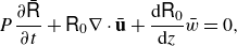 \begin{align}&\qquad\qquad\qquad\qquad\qquad\quad P \frac {\partial \bar {\textsf{R}}}{\partial t} + \textsf{R}_0 \nabla \cdot \bar {\textbf u} + \frac {{\rm d}\textsf{R}_0}{{\rm d} z} \bar {w} = 0, \end{align}
 \begin{align}&\qquad\qquad \textsf{R}_0\frac {\partial \bar {\textbf u}}{\partial t} - \textsf{M}_0 \nabla ^2 \bar {\textbf u} -\frac 13 \textsf{M}_0 \nabla \left ( \nabla \cdot \bar {\textbf u} \right ) + \nabla \bar p +G \bar {\textsf{R}} {\textbf {e}}_z - \frac {{\rm d}\textsf{M}_0}{{\rm d} z} \boldsymbol{\varepsilon }=0, \end{align}
 \begin{align}&\qquad\quad \textsf{H}_0 \left (P \frac {\partial \bar {T}}{\partial t} + \frac {{\rm d} T_0}{{\rm d} z}\bar {w}\right ) -\textsf{K}_0 \nabla ^2 \bar {T} -\bar {\textsf{K}}\frac {{\rm d}^2 T_0}{{\rm d} z^2} - \frac {{\rm d} T_0}{{\rm d} z}\frac {\partial \bar {\textsf{K}}}{\partial z} - \frac {{\rm d} \textsf{K}_0}{{\rm d} z}\frac {\partial \bar {T}}{\partial z} = 0, \end{align}
 \begin{align}& PL^{-1}\frac {\partial \bar {\phi }}{\partial t} + \phi _0 L^{-1} \nabla \!\cdot \bar {\textbf u} +\frac {{\rm d}\phi _0}{{\rm d} z}\!\left (\!L^{-1}\bar {w}-\eta \frac {\partial \bar {T}}{\partial z}\right ) - \eta \phi _0\nabla ^2 \bar T -\eta \frac {\partial }{\partial z} \!\left (\frac {{\rm d} T_0}{{\rm d} z} \bar \phi \right ) - \nabla ^2 \bar \phi =0, \end{align}
where
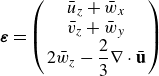 \begin{align} \displaystyle \boldsymbol{\varepsilon } = \left ( \begin{array}{c} \displaystyle \bar {u}_z+\bar {w}_x \\ \displaystyle \bar {v}_z+\bar {w}_y\\ \displaystyle 2 \bar {w}_z -\frac 23 \nabla \cdot \bar {\textbf u} \\ \end{array} \right ) \end{align}
is a vector containing the two off-diagonal and one diagonal components of the strain rate associated with the $z$
-direction.
$z$
-direction.
The linearised boundary conditions at $z=0$
are
$z=0$
are
 \begin{equation} \bar {\textbf{u}}=0,\quad \textsf{K}_0\frac {\partial \bar {T}}{\partial z} + \bar {\textsf{K}}\frac {{\rm d} T_0}{{\rm d} z} = 0,\quad \eta \phi _0 \frac {\partial \bar {T}}{\partial z} + \eta \frac {{\rm d} T_0}{{\rm d} z} \bar {\phi } + \frac {\partial \bar {\phi }}{\partial z}=0. \end{equation}
Note that (3.3a ), (3.3b ), (3.3c ), and (3.3d ) represent the linearised versions of the continuity, three-dimensional momentum conservation, energy and mass diffusion equations, respectively.
The linearised boundary conditions at $z=1$
are
$z=1$
are
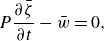 \begin{align}&\qquad\qquad\qquad\qquad\qquad P\frac {\partial \bar {\zeta }}{\partial t} - \bar {w} =0, \end{align}
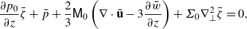 \begin{align}&\qquad\quad \frac {\partial p_0}{\partial z}\bar {\zeta } + \bar {p} + \frac {2}{3} \textsf{M}_0\left ( \nabla \cdot \bar {\textbf u} - 3 \frac {\partial \bar {w}}{\partial z}\right ) + \Sigma _0 \nabla _\perp ^2 \bar {\zeta } = 0, \end{align}
 \begin{align}& M_S \left (\nabla _\perp \bar {\phi }+\frac {{\rm d}\phi _0}{{\rm d} z}\nabla _\perp \bar\zeta \right ) + M_T \left (\nabla _\perp \bar {T}+\frac {{\rm d}T_0}{{\rm d} z}\nabla _\perp \bar\zeta \right ) + \textsf{M}_0 \boldsymbol{\varepsilon }_\perp = 0, \end{align}
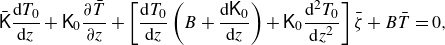 \begin{align}&\,\, \bar {\textsf{K}}\frac {{\rm d} T_0}{{\rm d} z} + \textsf{K}_0\frac {\partial \bar {T}}{\partial z} + \left [\frac {{\rm d} T_0}{{\rm d} z} \left (B+ \frac {{\rm d} \textsf{K}_0}{{\rm d} z}\right )+ \textsf{K}_0 \frac {{\rm d}^2T_0}{{\rm d} z^2}\right ] \bar {\zeta } + B \bar {T} =0, \end{align}
 \begin{align}& \frac {\partial \bar {\phi }}{\partial z}+ \left [\eta \frac {{\rm d} T_0}{{\rm d} z} \frac {{\rm d} \phi _0}{{\rm d} z} + \eta \phi _0\frac {{\rm d}^2 T_0}{{\rm d} z^2} + \frac {{\rm d}^2\phi _0}{{\rm d} z^2}\right ] \bar {\zeta } + \eta \frac {{\rm d} T_0}{{\rm d} z} \bar {\phi } + \eta \phi _0 \frac {\partial \bar {T}}{\partial z} = 0, \end{align}
where $\displaystyle \nabla _\perp \equiv \Big (\frac {\partial }{\partial x}, \frac {\partial }{\partial y} \Big)^\intercal$
and
$\displaystyle \nabla _\perp \equiv \Big (\frac {\partial }{\partial x}, \frac {\partial }{\partial y} \Big)^\intercal$
and
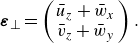 \begin{align} \displaystyle \boldsymbol{\varepsilon }_\perp = \left ( \begin{array}{c} \displaystyle \bar {u}_z+\bar {w}_x \\ \displaystyle \bar {v}_z+\bar {w}_y \\ \end{array} \right ). \end{align}
Equations (3.5a
), (3.5b
), (3.5c
), (3.5d
), and (3.5e
) represent the linearised versions of the kinematic, balance of normal stresses, two-dimensional balance of tangential stresses, heat and mass fluxes boundary conditions, respectively. In what follows, we constrain our study to the two-dimensional (2-D) case in the $x{-}z$
plane.
$x{-}z$
plane.
By applying the $\nabla \times$
operator to the momentum conservation equations and differentiating the normal stress balance boundary condition along the interface followed by substituting there the pressure gradient components obtained from the momentum conservation equations, we completely eliminate the pressure from the momentum conservation equations.
$\nabla \times$
operator to the momentum conservation equations and differentiating the normal stress balance boundary condition along the interface followed by substituting there the pressure gradient components obtained from the momentum conservation equations, we completely eliminate the pressure from the momentum conservation equations.
Normal perturbation modes are introduced in the form
 \begin{equation} \left (\bar u, \bar {w}, \bar {T}, \bar {\phi }, \bar {\zeta } ; \bar {\textsf{X}}\right )\left (x,z,t\right ) = \left (u(z), w(z),\theta (z),\varphi (z),\zeta ; \textsf{X}\right )\exp (ikx+\lambda t), \end{equation}
where $u,\, w,\, \theta, $ $\varphi, $ $\zeta $
, and
$\zeta $
, and $\textsf{X} \equiv (\textsf{R}(z),\textsf{M}(z), \textsf{K}(z), \textsf{H}(z) )$
are the amplitudes of the horizontal and vertical fluid velocity components, temperature, concentration, interfacial deformation and material properties (all expressed via
$\textsf{X} \equiv (\textsf{R}(z),\textsf{M}(z), \textsf{K}(z), \textsf{H}(z) )$
are the amplitudes of the horizontal and vertical fluid velocity components, temperature, concentration, interfacial deformation and material properties (all expressed via $\varphi$
) perturbations, respectively, with
$\varphi$
) perturbations, respectively, with $k$
and
$k$
and $\lambda$
representing the wavenumber and the growth rate of the disturbances, respectively. In this representation, positive and negative values of the real part of
$\lambda$
representing the wavenumber and the growth rate of the disturbances, respectively. In this representation, positive and negative values of the real part of $\lambda$
correspond to instability and stability regimes of the system, respectively. We note that
$\lambda$
correspond to instability and stability regimes of the system, respectively. We note that $\textsf{X}$
represents the material properties of the nanofluid which are concentration-dependent and does not contain independent variables following (3.2).
$\textsf{X}$
represents the material properties of the nanofluid which are concentration-dependent and does not contain independent variables following (3.2).
The resulting eigenvalue problem which determines the growth rate $\lambda$
of the disturbance as a function of its wavenumber
$\lambda$
of the disturbance as a function of its wavenumber $k$
and the rest of the problem parameters reads
$k$
and the rest of the problem parameters reads
 \begin{align}&\qquad\qquad\qquad \textsf{R}_0 \left (w^{\prime }+i k u\right )+\lambda P \textsf{R} + w \textsf{R}_0^{\prime }=0, \end{align}
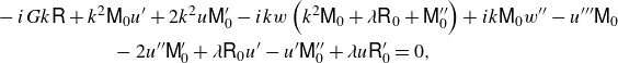 \begin{align}& -i G k \textsf{R} + k^2 \textsf{M}_0 u^{\prime } + 2 k^2 u \textsf{M}_0^{\prime } - i k w \left (k^2 \textsf{M}_0 + \lambda \textsf{R}_0 +\textsf{M}_0^{\prime \prime } \right )+i k \textsf{M}_0 w^{\prime \prime }-u^{\prime \prime \prime } \textsf{M}_0 \notag \\&\qquad\qquad\qquad -2 u^{\prime \prime } \textsf{M}_0^{\prime } + \lambda \textsf{R}_0 u^{\prime } - u^{\prime } \textsf{M}_0^{\prime \prime }+\lambda u \textsf{R}_0^{\prime } = 0, \end{align}
 \begin{align}&\qquad -T_0^{\prime \prime } \textsf{K} + \theta \left (k^2 \textsf{K}_{0} + \lambda P \textsf{H}_{0} \right )+T_0^{\prime } \left (w \textsf{H}_{0} - \textsf{K}^\prime \right )-\textsf{K}_{0} \theta ^{\prime \prime } - \textsf{K}_{0}^{\prime } \theta ^{\prime } = 0, \end{align}
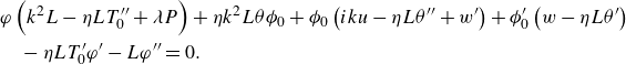 \begin{align}& \varphi \left (k^2 L-\eta L T_0^{\prime \prime } + \lambda P\right )+\eta k^2 L \theta \phi _0 + \phi _0 \left (i k u - \eta L \theta ^{\prime \prime } + w^{\prime } \right )+\phi _0^{\prime } \left (w - \eta L \theta ^{\prime } \right )\notag\\&\quad-\eta L T_0^{\prime } \varphi ^{\prime } - L \varphi ^{\prime \prime } =0. \end{align}
The boundary conditions at $z=0$
are
$z=0$
are
 \begin{equation} \textbf{u} = \left (a \phi _m \phi _0+1\right ) \theta ^{\prime } + a\phi _m T_0^{\prime } \varphi = \eta \phi _0 \theta ^{\prime } + \eta T_0^{\prime } \varphi + \varphi ^{\prime }=0. \end{equation}
The boundary conditions at the deformable interface $z=h$
projected onto
$z=h$
projected onto $z=1$
are
$z=1$
are
 \begin{align}&\qquad\qquad\qquad\qquad\qquad\qquad \zeta \lambda P-w =0, \end{align}
 \begin{align}& T_0^{\prime } \left (a\phi _m \left (\zeta \phi _0^{\prime } + \varphi \right )+B \zeta \right )+\left ( a\phi _m \phi _0 +1\right ) \theta ^{\prime } + \zeta T_0^{\prime \prime } \left (a\phi _m \phi _0 +1\right )+B \theta =0, \end{align}
 \begin{align}&\qquad\qquad\quad \zeta \phi _0^{\prime \prime } + \eta \phi _0 \left (\theta ^{\prime } + \zeta T_0^{\prime \prime }\right )+\eta T_0^{\prime } \left (\zeta \phi _0^{\prime } + \varphi \right )+\varphi ^{\prime } = 0, \end{align}
 \begin{align}&\qquad\qquad k M_S \left (\zeta \phi _0^{\prime } + \varphi \right )+k M_T \left (\zeta T_0^{\prime } + \theta \right )+ \textsf{M}_{0} \left (k w-i u^{\prime }\right )=0, \end{align}
 \begin{align}& i \zeta k^3 \Sigma _0+u \left (2 k^2 \textsf{M}_{0} + \lambda \textsf{R}_{0} \right )+i \left (-\zeta k p_0^{\prime } + k \textsf{M}_{0} w^{\prime } - k \textsf{M} _{0}^{\prime } w+i \textsf{M}_{0} u^{\prime \prime } + i \textsf{M}_{0}^{\prime } u^{\prime }\right )=0. \end{align}
Here and on, primes denote differentiation with respect to $z$
. We reiterate that
$z$
. We reiterate that $\textsf{R}_0,\textsf{M}_0, \textsf{K}_0, \textsf{H}_0$
represent the base state values of the thermophysical properties of the system given by (3.2), whereas
$\textsf{R}_0,\textsf{M}_0, \textsf{K}_0, \textsf{H}_0$
represent the base state values of the thermophysical properties of the system given by (3.2), whereas $\textsf{R},\textsf{M}, \textsf{K}, \textsf{H}$
are the amplitudes of their respective disturbances depending on
$\textsf{R},\textsf{M}, \textsf{K}, \textsf{H}$
are the amplitudes of their respective disturbances depending on $z$
. Finally, we note that normal perturbations imposed on the bulk concentration
$z$
. Finally, we note that normal perturbations imposed on the bulk concentration $\phi$
automatically preserve the average bulk concentration due to periodicity of the
$\phi$
automatically preserve the average bulk concentration due to periodicity of the $x$
-component
$x$
-component $\exp (ikx)$
of the perturbation
$\exp (ikx)$
of the perturbation $\bar \phi$
.
$\bar \phi$
.
4. Results
4.1. Numerical procedure
To precondition the eigenvalue problem equations (3.7) for a more efficient numerical solution, we substitute the expression of the perturbed longitudinal velocity component $u$
from (3.7a
) into the rest of the equations of the eigenvalue problem (3.7). We also extract the expression for the interfacial deformation
$u$
from (3.7a
) into the rest of the equations of the eigenvalue problem (3.7). We also extract the expression for the interfacial deformation $\zeta$
from (3.7j
) and substitute it into the rest of the boundary conditions at
$\zeta$
from (3.7j
) and substitute it into the rest of the boundary conditions at $z=1$
. Hence, our eigenvalue problem is formulated in terms of
$z=1$
. Hence, our eigenvalue problem is formulated in terms of $w, \theta, \varphi$
and it is treated numerically in this format. We note here that in the case of the non-deformable interface considered in § 4.4, the pressure will be eliminated without substituting its gradients into the normal stress boundary condition, since the latter is redundant, and
$w, \theta, \varphi$
and it is treated numerically in this format. We note here that in the case of the non-deformable interface considered in § 4.4, the pressure will be eliminated without substituting its gradients into the normal stress boundary condition, since the latter is redundant, and $\zeta =0$
is imposed.
$\zeta =0$
is imposed.
The numerical solution of the linear eigenvalue problem given by (3.7), or any of its simplified versions discussed in what follows, is obtained using the open-source code developed by Pearce et al. (Reference Pearce, Heil, Jensen, Jones and Prokop2018). It is based on the shooting method and numerical construction of the complex-valued Evans function (Evans & Feroe Reference Evans and Feroe1977) whose roots represent the eigenvalues of the given problem. The solution is initiated by specifying the range where the roots of the Evans function are searched and adjusted if needed.
Alternatively, it is possible to locate the eigenvalues graphically by sampling the Evans function on the complex plane of $\lambda$
, and by doing so, one obtains contour plots of the Evans function for a specified range of
$\lambda$
, and by doing so, one obtains contour plots of the Evans function for a specified range of $(\lambda _r,\lambda _i)$
, where
$(\lambda _r,\lambda _i)$
, where $\lambda _r \equiv \Re (\lambda )$
and
$\lambda _r \equiv \Re (\lambda )$
and $\lambda _i \equiv \Im (\lambda )$
. Then, the intersection points of the contour lines with the reference point of the plane or with the axis
$\lambda _i \equiv \Im (\lambda )$
. Then, the intersection points of the contour lines with the reference point of the plane or with the axis $\lambda _i=0$
are traced. These intersection points represent the eigenvalues of the problem among which one finds the eigenvalue relevant for the onset of either monotonic or oscillatory instability of the system, respectively. However, this approach is computationally costly, and the available routine to locate roots of the Evans function is preferable and is therefore used in our investigation.
$\lambda _i=0$
are traced. These intersection points represent the eigenvalues of the problem among which one finds the eigenvalue relevant for the onset of either monotonic or oscillatory instability of the system, respectively. However, this approach is computationally costly, and the available routine to locate roots of the Evans function is preferable and is therefore used in our investigation.
The shooting method is implemented by solving the differential equations of the eigenvalue problem (3.7) or any of their simplified versions discussed below as a boundary-value problem using the compound matrix method (Ng & Reid Reference Ng and Reid1979) to construct the Evans function by satisfying the boundary conditions separately at each of the two endpoints $z=0$
and
$z=0$
and $z=1$
, and then matching the solutions at the interim point either in the middle of the domain or elsewhere.
$z=1$
, and then matching the solutions at the interim point either in the middle of the domain or elsewhere.
To verify the convergence of the computation procedure, we check the accuracy of the results by changing the number of decimal digits used in the computation and by varying the matching point where the Evans function is created. We find that the values obtained for the critical values of the Marangoni number for various parameter sets of the problem based on three different matching points within the layer domain $ 0 \leqslant z \leqslant 1$
, namely
$ 0 \leqslant z \leqslant 1$
, namely $z=1/3,\,z=1/2$
and
$z=1/3,\,z=1/2$
and $z=2/3$
, converge up to the third digit.
$z=2/3$
, converge up to the third digit.
In what follows, we concentrate on physical systems in which the solvent is water. Therefore, the corresponding value of the Prandtl number is taken in our investigation as $P=7$
. The value of the Lewis number used in most cases discussed below is
$P=7$
. The value of the Lewis number used in most cases discussed below is $L=10^{-3}$
, which is quite representative for a moderately dense nanosuspension mixture. For reference, in the case of nanoparticles of diameter
$L=10^{-3}$
, which is quite representative for a moderately dense nanosuspension mixture. For reference, in the case of nanoparticles of diameter $d_p^*\sim 10$
nm, the Lewis number estimated using the Stokes–Einstein formula (2.4), is
$d_p^*\sim 10$
nm, the Lewis number estimated using the Stokes–Einstein formula (2.4), is $L = 4.22\times 10^{-4}$
when the solvent temperature is
$L = 4.22\times 10^{-4}$
when the solvent temperature is $T^*=300\,$
K. Furthermore, we consider the range of the values for the Soret coefficient
$T^*=300\,$
K. Furthermore, we consider the range of the values for the Soret coefficient $\eta \in (0.31,3.1)$
corresponding to the temperature drop of
$\eta \in (0.31,3.1)$
corresponding to the temperature drop of $\Delta T^* \in (1,10)$
K across the layer. In addition, we determine the dimensionless parameters related to nanoparticle density via
$\Delta T^* \in (1,10)$
K across the layer. In addition, we determine the dimensionless parameters related to nanoparticle density via
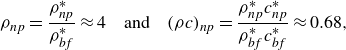 \begin{align} \rho _{np} = \frac {\rho _{np}^*}{\rho _{bf}^*}\approx 4\quad \text{and}\quad (\rho c)_{np} = \frac {\rho _{np}^*c_{np}^*}{\rho _{bf}^*c_{bf}^*}\approx 0.68, \end{align}
which corresponds to alumina nanoparticles in water, also taking $a=7.47$
in this investigation, except for § 4.4 where the parameter
$a=7.47$
in this investigation, except for § 4.4 where the parameter $a$
is changing.
$a$
is changing.
Before we present the results of the linear stability analysis, we note that the equilibrium surface tension $\sigma ^\ast _r$
ranges for aqueous solutions from
$\sigma ^\ast _r$
ranges for aqueous solutions from ${\sim} 10^{-3} \ \textrm {to}\ 30 \times 10^{-3}$
Nm−1 (De Wit, Gallez & Christov Reference De Wit, Gallez and Christov1994); therefore, the dimensionless surface tension for a layer of density
${\sim} 10^{-3} \ \textrm {to}\ 30 \times 10^{-3}$
Nm−1 (De Wit, Gallez & Christov Reference De Wit, Gallez and Christov1994); therefore, the dimensionless surface tension for a layer of density $\rho ^\ast _{bf}=10^{3}\,\text{kg m}^{-3}$
, viscosity
$\rho ^\ast _{bf}=10^{3}\,\text{kg m}^{-3}$
, viscosity $\mu ^\ast _{bf}=10^{-3}\,\text{kg (m} \cdot \text{s)}^{-1}$
, thermal diffusivity
$\mu ^\ast _{bf}=10^{-3}\,\text{kg (m} \cdot \text{s)}^{-1}$
, thermal diffusivity $\kappa ^\ast _{bf}=0.146\times 10^{-6}\,\text{m}^2 \, \text{s}^{-1}$
and thickness
$\kappa ^\ast _{bf}=0.146\times 10^{-6}\,\text{m}^2 \, \text{s}^{-1}$
and thickness $h_0^\ast =10^{-4}\,\text{m}$
is approximately
$h_0^\ast =10^{-4}\,\text{m}$
is approximately $\Sigma _0=2\times 10^{4}$
. Similarly, the modified Galileo number for the terrestrial gravity of
$\Sigma _0=2\times 10^{4}$
. Similarly, the modified Galileo number for the terrestrial gravity of $g^\ast =9.81\,\text{m s}^{-2}$
yields
$g^\ast =9.81\,\text{m s}^{-2}$
yields $G=67.2$
for
$G=67.2$
for $h^\ast _0=10^{-4}$
m and
$h^\ast _0=10^{-4}$
m and $G \sim 10^{-4}$
for
$G \sim 10^{-4}$
for $h^\ast _0=10^{-6}$
m. A list of typical values of the thermophysical properties of the nanofluid and the dimensionless numbers is given in table 1.
$h^\ast _0=10^{-6}$
m. A list of typical values of the thermophysical properties of the nanofluid and the dimensionless numbers is given in table 1.
Table 1. Parameter nomenclature and their typical values used in this investigation.
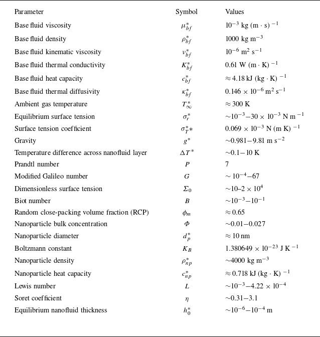
4.2. Cooling at the substrate $(\mathcal{Q} = -1)$

In this section, we study the onset of the thermosolutocapillary instability when the nanofluid layer is cooled at the substrate. Studies of this configuration for pure fluids are quite rare in the literature (Deissler & Oron Reference Deissler and Oron1992; Oron & Rosenau Reference Oron and Rosenau1992; Burgess et al. Reference Burgess, Juel, McCormick, Swift and Swinney2001; Alexeev & Oron Reference Alexeev and Oron2007). Recently, Sarma & Mondal (Reference Sarma and Mondal2021b ) studied thermosolutal Marangoni instability in a layer of a viscoelastic binary fluid in the presence of the Soret effect. They also presented some results for the limiting case of a Newtonian fluid associated with a zero Deborah number. However, due to the fact they used a linearised version for the Soret component of the mass flux along with constant thermophysical properties of the fluid in contradistiction to the particle concentration-dependent Soret coefficient and other thermophysical properties of the nanofluid used in this paper, any quantitative comparison between the results is impossible. However, a qualitative comparison is possible and it will be made at the end of this section.
First, it must be clear that in the configuration at hand, thermocapillarity is stabilising for $M_T\gt 0$
, because any small elevation (depression) at the layer interface will have a higher (lower) temperature than in its vicinity along the interface, and thermocapillary interfacial tractions will lead to flattening of the interface. Figure 2(a) shows a stably stratified concentration profile and this configuration suggests a possibility of the emergence of the solutocapillary instability. Indeed, we find that solutocapillarity destabilises the system when the layer is cooled at the substrate and figure 4(a) displays the neutral curves for the pure monotonic solutocapillary instability for varying Biot numbers
$M_T\gt 0$
, because any small elevation (depression) at the layer interface will have a higher (lower) temperature than in its vicinity along the interface, and thermocapillary interfacial tractions will lead to flattening of the interface. Figure 2(a) shows a stably stratified concentration profile and this configuration suggests a possibility of the emergence of the solutocapillary instability. Indeed, we find that solutocapillarity destabilises the system when the layer is cooled at the substrate and figure 4(a) displays the neutral curves for the pure monotonic solutocapillary instability for varying Biot numbers $B$
. We note that the solutal Marangoni number
$B$
. We note that the solutal Marangoni number $M_S$
exhibits non-monotonic variation with the wavenumber
$M_S$
exhibits non-monotonic variation with the wavenumber $k$
. We also infer that the variation of the Biot number does not significantly affect the critical value of the solutal Marangoni number. However, we note that the neutral curves display the emergence of two local minima, one of them is associated with a low value of the wavenumber
$k$
. We also infer that the variation of the Biot number does not significantly affect the critical value of the solutal Marangoni number. However, we note that the neutral curves display the emergence of two local minima, one of them is associated with a low value of the wavenumber $k$
, whereas the second one belongs to the finite range of
$k$
, whereas the second one belongs to the finite range of $k$
. Both of them are clearly seen in the neutral curve for
$k$
. Both of them are clearly seen in the neutral curve for $B=0.01$
in figure 4(a).
$B=0.01$
in figure 4(a).
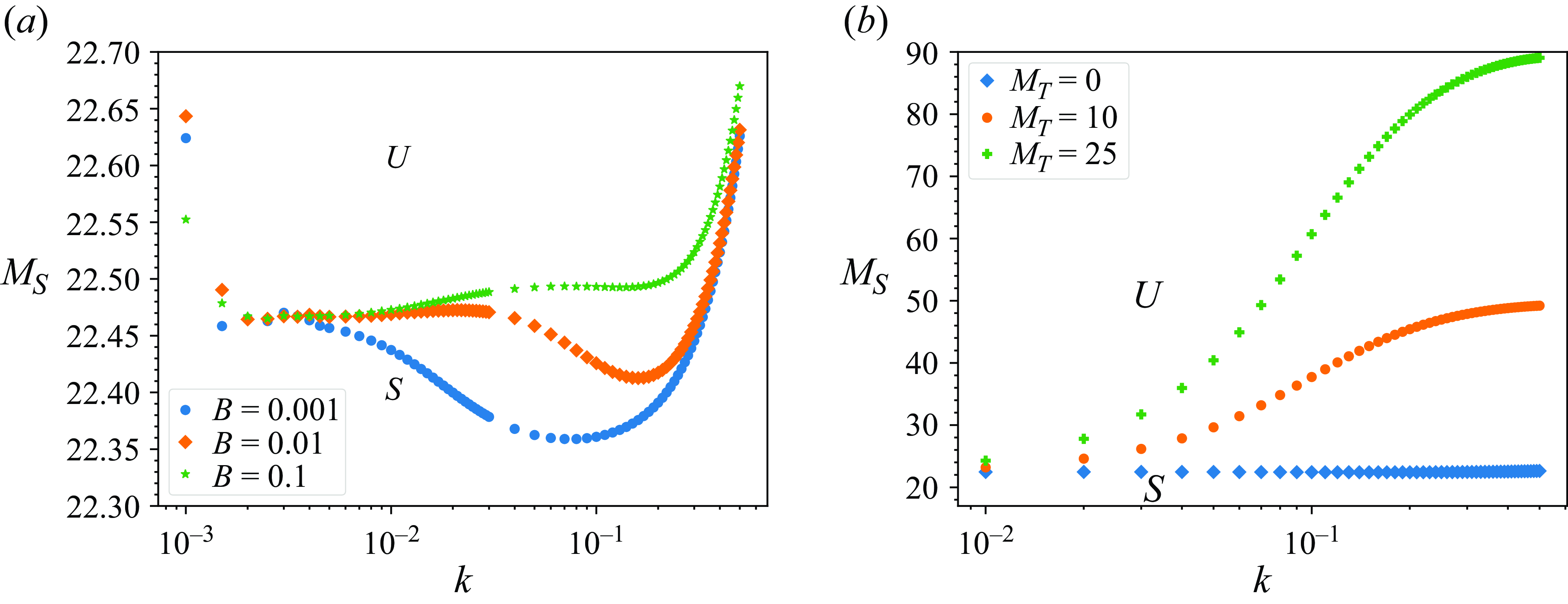
Figure 4. Monotonic solutocapillary instability in the case of cooling at the substrate $\mathcal{Q}=-1$
at
$\mathcal{Q}=-1$
at $\Phi =0.01, a=7.47, \eta =0.31, L=10^{-3}, \Sigma _0\approx 2\times 10^{4}$
and
$\Phi =0.01, a=7.47, \eta =0.31, L=10^{-3}, \Sigma _0\approx 2\times 10^{4}$
and $G=6.71$
. (a) Neutral curves
$G=6.71$
. (a) Neutral curves $M_S(k)$
for the pure solutocapillarity instability,
$M_S(k)$
for the pure solutocapillarity instability, $M_T = 0$
, versus the wavenumber
$M_T = 0$
, versus the wavenumber $k$
for various Biot numbers
$k$
for various Biot numbers $B$
. (b) Neutral curves
$B$
. (b) Neutral curves $M_S(k)$
for various values of
$M_S(k)$
for various values of $M_T$
with
$M_T$
with $B=0.01$
. The rise of the neutral curves with an increase in
$B=0.01$
. The rise of the neutral curves with an increase in $M_T$
illustrates a stabilising effect of thermocapillarity on the monotonic solutocapillary instability. In both panels, the symbols
$M_T$
illustrates a stabilising effect of thermocapillarity on the monotonic solutocapillary instability. In both panels, the symbols $U$
and
$U$
and $S$
denote the unstable and stable domains of the system, respectively.
$S$
denote the unstable and stable domains of the system, respectively.
In addition, we note that when the layer is cooled at the substrate, the temperature base state increases with height $z$
, as shown in figure 2(b). This implies that at the interfacial hump, the temperature is higher than that at its depression. Thus, the emerging thermocapillary shear stress will lead to fluid flow from the hump into the depression, causing the tendency of interface flattening and therefore indicating a tendency to stabilisation (Deissler & Oron Reference Deissler and Oron1992; Alexeev & Oron Reference Alexeev and Oron2007). Figure 4(b) illustrates a significant stabilisation effect imparted by thermocapillarity on the solutocapillary instability threshold. In the range of
$z$
, as shown in figure 2(b). This implies that at the interfacial hump, the temperature is higher than that at its depression. Thus, the emerging thermocapillary shear stress will lead to fluid flow from the hump into the depression, causing the tendency of interface flattening and therefore indicating a tendency to stabilisation (Deissler & Oron Reference Deissler and Oron1992; Alexeev & Oron Reference Alexeev and Oron2007). Figure 4(b) illustrates a significant stabilisation effect imparted by thermocapillarity on the solutocapillary instability threshold. In the range of $M_T$
presented in this figure, the critical value of
$M_T$
presented in this figure, the critical value of $M_S$
slightly increases with
$M_S$
slightly increases with $M_T$
; however, the finite-wave modes are strongly stabilised with an increase in
$M_T$
; however, the finite-wave modes are strongly stabilised with an increase in $M_T$
.
$M_T$
.
Figure 5(a) shows that the threshold value of the solutal Marangoni number $M_S$
in the pure solutocapillary instability increases linearly with the modified Galileo number
$M_S$
in the pure solutocapillary instability increases linearly with the modified Galileo number $G$
. However, as we already mentioned, the neutral curves
$G$
. However, as we already mentioned, the neutral curves $M_S(k)$
exhibit two minima: one of them,
$M_S(k)$
exhibit two minima: one of them, $M_S=m_f$
, is in the finite-wave domain, whereas the second one,
$M_S=m_f$
, is in the finite-wave domain, whereas the second one, $M_S=m_l$
, belongs to the long-wave domain. The relative importance of these two minima with respect to the onset of the purely solutocapillary instability is now under scrutiny. The inset of figure 5(a) shows that in the domain of intermediate values of the modified Galileo number
$M_S=m_l$
, belongs to the long-wave domain. The relative importance of these two minima with respect to the onset of the purely solutocapillary instability is now under scrutiny. The inset of figure 5(a) shows that in the domain of intermediate values of the modified Galileo number $14.8\leqslant G\leqslant 66.6$
, the long-wave minimum
$14.8\leqslant G\leqslant 66.6$
, the long-wave minimum $M_S=m_l$
corresponding to the deformational mode prevails over the finite-wave minimum
$M_S=m_l$
corresponding to the deformational mode prevails over the finite-wave minimum $M_S=m_f$
, namely
$M_S=m_f$
, namely $m_l\lt m_f$
, and corresponds to the instability onset. In addition, we find that in the rest of the
$m_l\lt m_f$
, and corresponds to the instability onset. In addition, we find that in the rest of the $G$
range, i.e. for relatively low and sufficiently high values of
$G$
range, i.e. for relatively low and sufficiently high values of $G$
,
$G$
, $m_l\gt m_f$
, and the finite-wave solutocapillary instability emerges. VanHook et al. (Reference VanHook, Schatz, Swift, McCormick and Swinney1997) and Golovin, Nepomnyashchy & Pismen (Reference Golovin, Nepomnyashchy and Pismen1997) observed an analogous effect of the competition between the long-wave deformational and finite-wave pattern forming modes for the thermocapillary instability in a layer with a deformable interface. Figure 5(b) displays the variation of the critical wavenumber
$m_l\gt m_f$
, and the finite-wave solutocapillary instability emerges. VanHook et al. (Reference VanHook, Schatz, Swift, McCormick and Swinney1997) and Golovin, Nepomnyashchy & Pismen (Reference Golovin, Nepomnyashchy and Pismen1997) observed an analogous effect of the competition between the long-wave deformational and finite-wave pattern forming modes for the thermocapillary instability in a layer with a deformable interface. Figure 5(b) displays the variation of the critical wavenumber $k_c$
with
$k_c$
with $G$
. We note that the critical wavenumber
$G$
. We note that the critical wavenumber $k_c$
for the finite-wave minimum
$k_c$
for the finite-wave minimum $M_T=m_f$
exhibits two distinct domains of variation with
$M_T=m_f$
exhibits two distinct domains of variation with $G$
. For moderate values of the modified Galileo number
$G$
. For moderate values of the modified Galileo number $G$
,
$G$
, $k_c$
varies slowly; however, for sufficiently large values of
$k_c$
varies slowly; however, for sufficiently large values of $G$
, the critical wave number
$G$
, the critical wave number $k_c$
sharply increases. The inset of figure 5(b) shows a decrease in the critical wavenumber
$k_c$
sharply increases. The inset of figure 5(b) shows a decrease in the critical wavenumber $k_c$
of the long-wave instability corresponding to the minimum
$k_c$
of the long-wave instability corresponding to the minimum $M_S=m_l$
with
$M_S=m_l$
with $G$
.
$G$
.

Figure 5. Onset of a purely solutocapillary monotonic instability in the case of cooling at the substrate $\mathcal{Q}=-1$
at
$\mathcal{Q}=-1$
at $\Phi =0.01,\,a=7.47,\,\eta =0.31,\,L=10^{-3},\,M_T = 0,\,\Sigma _0\approx 2\times 10^{4}$
and
$\Phi =0.01,\,a=7.47,\,\eta =0.31,\,L=10^{-3},\,M_T = 0,\,\Sigma _0\approx 2\times 10^{4}$
and $B = 0.01$
. (a) Variation of the critical value of the solutal Marangoni number
$B = 0.01$
. (a) Variation of the critical value of the solutal Marangoni number $M_S$
versus the modified Galileo number
$M_S$
versus the modified Galileo number $G$
that shows both the finite-wave range minimum
$G$
that shows both the finite-wave range minimum $M_S=m_f$
and the long-wave minimum
$M_S=m_f$
and the long-wave minimum $M_S=m_l$
; the inset presents the variation of the difference
$M_S=m_l$
; the inset presents the variation of the difference $m_l-m_f$
versus
$m_l-m_f$
versus $G$
. FW and LW stand for domains of finite-wave and long-wave instability, respectively. (b) Variation of the critical wavenumber
$G$
. FW and LW stand for domains of finite-wave and long-wave instability, respectively. (b) Variation of the critical wavenumber $k_c$
with
$k_c$
with $G$
; the inset shows a decrease in the critical wavenumber
$G$
; the inset shows a decrease in the critical wavenumber $k_c$
corresponding to the long-wave minimum
$k_c$
corresponding to the long-wave minimum $M_S=m_l$
with
$M_S=m_l$
with $G$
. The symbols
$G$
. The symbols $U$
and
$U$
and $S$
denote the unstable and stable domains of the system, respectively.
$S$
denote the unstable and stable domains of the system, respectively.
Figure 6(a) shows that in the case of a purely solutocapillary instability, the critical solutal Marangoni number $M_S$
monotonically increases with the dimensionless surface tension number
$M_S$
monotonically increases with the dimensionless surface tension number $\Sigma _0$
when the rest of the parameters are fixed and saturates at a very high value of
$\Sigma _0$
when the rest of the parameters are fixed and saturates at a very high value of $\Sigma _0$
that corresponds to the non-deformable interface. Slightly above it, a dashed curve corresponding to the secondary minimum of the corresponding neutral curve is located. The critical value of
$\Sigma _0$
that corresponds to the non-deformable interface. Slightly above it, a dashed curve corresponding to the secondary minimum of the corresponding neutral curve is located. The critical value of $M_S$
is attained at the local minimum of the neutral curves corresponding to
$M_S$
is attained at the local minimum of the neutral curves corresponding to $M_S=m_f$
and varies weakly with
$M_S=m_f$
and varies weakly with $\Sigma _0$
. The variation of the critical wavenumber
$\Sigma _0$
. The variation of the critical wavenumber $k_c$
is non-monotonic with
$k_c$
is non-monotonic with $\Sigma _0$
in the finite but relatively low wavenumber range, as shown in figure 6(b), so the instability is finite-wave. The wavenumber corresponding to the secondary local minimum of the neutral curves
$\Sigma _0$
in the finite but relatively low wavenumber range, as shown in figure 6(b), so the instability is finite-wave. The wavenumber corresponding to the secondary local minimum of the neutral curves $M_S(k)=m_l$
remains almost unchanging with
$M_S(k)=m_l$
remains almost unchanging with $\Sigma _0$
and small,
$\Sigma _0$
and small, $k \approx 2.0 \times 10^{-3}$
; therefore, this secondary mode is long-wave.
$k \approx 2.0 \times 10^{-3}$
; therefore, this secondary mode is long-wave.
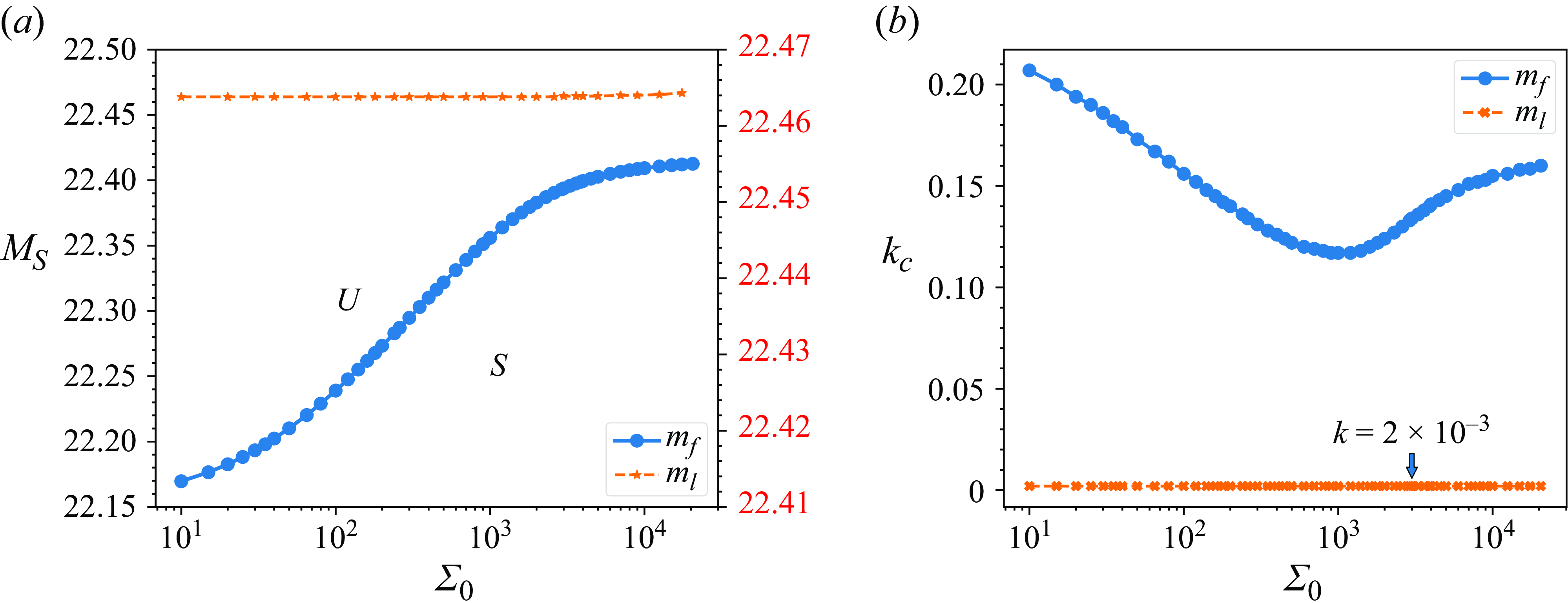
Figure 6. Variation of the onset of the pure solutocapillary monotonic instability with the dimensionless surface tension number $\Sigma _0$
for the case of cooling at the substrate
$\Sigma _0$
for the case of cooling at the substrate $\mathcal{Q}=-1$
at
$\mathcal{Q}=-1$
at $\Phi =0.01,\,a=7.47,\,\eta =0.31,\,L=10^{-3},\,M_T = 0,\,G=6.71$
and
$\Phi =0.01,\,a=7.47,\,\eta =0.31,\,L=10^{-3},\,M_T = 0,\,G=6.71$
and $B = 0.01$
. The
$B = 0.01$
. The $m_l$
and
$m_l$
and $m_f$
points correspond to the long-wave and finite-wave modes, respectively. The symbols
$m_f$
points correspond to the long-wave and finite-wave modes, respectively. The symbols $U$
and
$U$
and $S$
denote the unstable and stable domains of the system, respectively. (a) Variation of the values of the solutal Marangoni number
$S$
denote the unstable and stable domains of the system, respectively. (a) Variation of the values of the solutal Marangoni number $M_S$
corresponding to the two local minima
$M_S$
corresponding to the two local minima $M_S=m_l$
and
$M_S=m_l$
and $M_S=m_f$
of the neutral curves
$M_S=m_f$
of the neutral curves $M_S(k)$
. The instability threshold
$M_S(k)$
. The instability threshold $M_S$
increases with
$M_S$
increases with $\Sigma _0$
. The right vertical scale corresponds to
$\Sigma _0$
. The right vertical scale corresponds to $M_S$
related to the long-wave minimum
$M_S$
related to the long-wave minimum $M_S=m_l$
. (b) Variation of the wavenumbers corresponding to the two local minima of the neutral curves with
$M_S=m_l$
. (b) Variation of the wavenumbers corresponding to the two local minima of the neutral curves with $\Sigma _0$
. The critical wavenumber
$\Sigma _0$
. The critical wavenumber $k_c$
corresponding to the onset of the instability lies in the finite-wave range and varies non-monotonically with the dimensionless surface tension number
$k_c$
corresponding to the onset of the instability lies in the finite-wave range and varies non-monotonically with the dimensionless surface tension number $\Sigma _0$
. The wavenumber
$\Sigma _0$
. The wavenumber $k$
corresponding to the long-wave competing mode is almost constant with
$k$
corresponding to the long-wave competing mode is almost constant with $\Sigma _0$
.
$\Sigma _0$
.
We next study the variation of the onset of the pure solutocapillary instability with the averaged nanoparticle bulk concentration $\Phi$
. Figure 7(a) displays a significant monotonic decrease in the threshold value of the solutal Marangoni number
$\Phi$
. Figure 7(a) displays a significant monotonic decrease in the threshold value of the solutal Marangoni number $M_S$
(for both modes
$M_S$
(for both modes $m_f$
and
$m_f$
and $m_l$
) with an increase in
$m_l$
) with an increase in $\Phi$
. The reason for this effect is mainly due to the Soret effect whose strength is proportional to the local concentration
$\Phi$
. The reason for this effect is mainly due to the Soret effect whose strength is proportional to the local concentration $\phi$
. In the case of cooling at the substrate, the temperature gradient is directed upward; therefore, the Soret effect with
$\phi$
. In the case of cooling at the substrate, the temperature gradient is directed upward; therefore, the Soret effect with $\eta \gt 0$
drives the thermophoretic component of the mass flux downward and becomes stronger with an increase in the average particle concentration
$\eta \gt 0$
drives the thermophoretic component of the mass flux downward and becomes stronger with an increase in the average particle concentration $\Phi$
. This leads to a stronger decrease in particle concentration in the neighbourhood of the interface and to an enhanced decrease in local viscosity there with an increase in
$\Phi$
. This leads to a stronger decrease in particle concentration in the neighbourhood of the interface and to an enhanced decrease in local viscosity there with an increase in $\Phi$
. Thus, the critical solutal Marangoni number
$\Phi$
. Thus, the critical solutal Marangoni number $M_S$
driving the instability decreases with
$M_S$
driving the instability decreases with $\Phi$
.
$\Phi$
.
It is natural to observe such a decrease of the solutocapillary instability threshold for a nanofluid suspension or a mixture with a surfactant where the surface tension linearly decreases with the interfacial concentration (Morozov et al. Reference Morozov, Oron and Nepomnyashchy2014; Shklyaev & Nepomnyashchy Reference Shklyaev and Nepomnyashchy2017). However, for an inorganic salt where the surface tension increases with the interfacial concentration, the opposite behaviour could be observed (Oron & Nepomnyashchy Reference Oron and Nepomnyashchy2004). Further, we note that the critical wavenumber $k_c$
for the finite-wave minimum gradually increases with
$k_c$
for the finite-wave minimum gradually increases with $\Phi$
, whereas the wavenumber for the long-wave minimum remains almost constant around
$\Phi$
, whereas the wavenumber for the long-wave minimum remains almost constant around $k_c\approx 8\times 10^{-4}$
. Since the finite-wave minimum
$k_c\approx 8\times 10^{-4}$
. Since the finite-wave minimum $M_S=m_f$
remains always slightly below the long-wave one
$M_S=m_f$
remains always slightly below the long-wave one $M_S=m_l$
, the instability remains finite-wave, with the wavenumber variation shown in figure 7(b). We also find that the structure of the neutral curves remains unchanged with the variation of
$M_S=m_l$
, the instability remains finite-wave, with the wavenumber variation shown in figure 7(b). We also find that the structure of the neutral curves remains unchanged with the variation of $\Phi$
and a typical neutral curve is shown in the inset of figure 7(a).
$\Phi$
and a typical neutral curve is shown in the inset of figure 7(a).
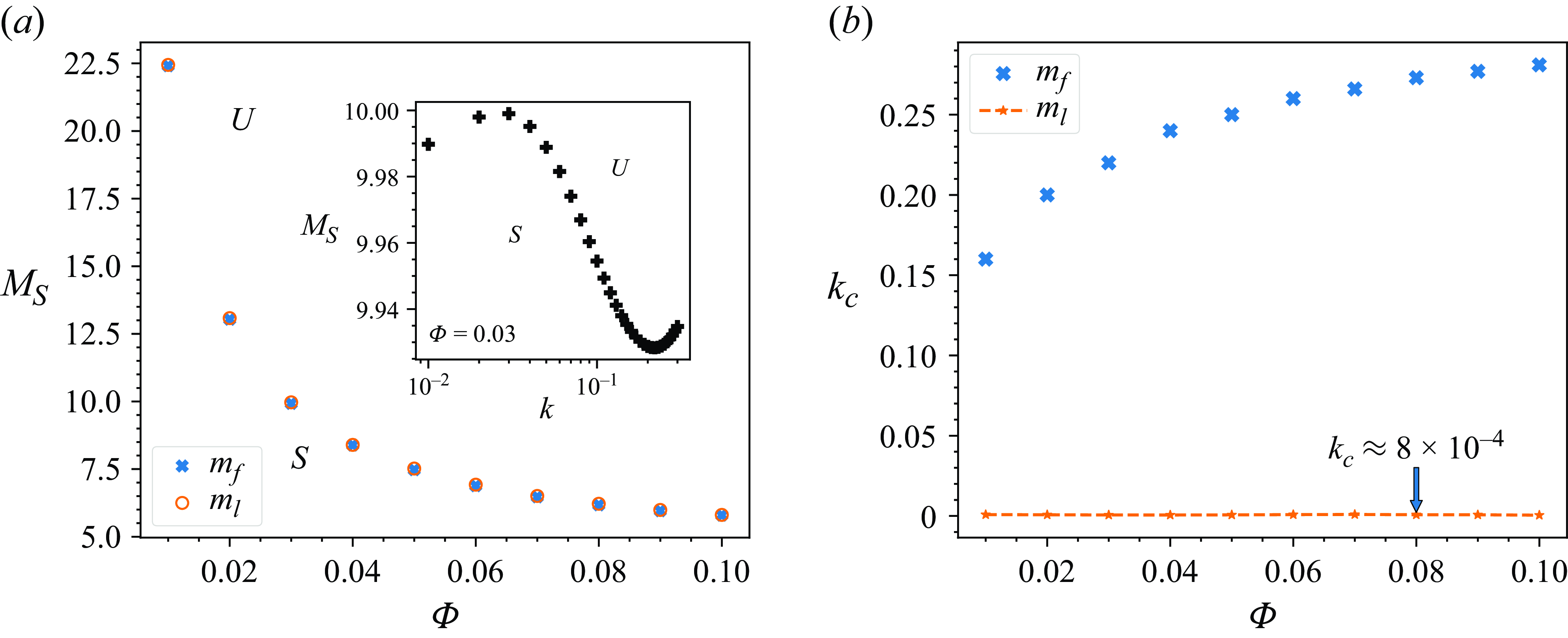
Figure 7. Variation of the onset of the pure solutocapillary monotonic instability with the averaged bulk nanoparticle concentration $\Phi$
for the case of cooling at the substrate
$\Phi$
for the case of cooling at the substrate $\mathcal{Q}=-1$
and
$\mathcal{Q}=-1$
and $a=7.47,\,\eta =0.31, L=10^{-3},\,M_T = 0,\,G=6.71,\,\Sigma _0=2\times 10^{4}$
and
$a=7.47,\,\eta =0.31, L=10^{-3},\,M_T = 0,\,G=6.71,\,\Sigma _0=2\times 10^{4}$
and $B = 0.01$
. (a) Variation of the two minimal values
$B = 0.01$
. (a) Variation of the two minimal values $M_S=m_f$
and
$M_S=m_f$
and $M_S=m_l$
of the neutral curves
$M_S=m_l$
of the neutral curves $M_S(k)$
. The inset shows the neutral curve for
$M_S(k)$
. The inset shows the neutral curve for $\Phi =0.03$
. (b) Variation of the wavenumbers corresponding to the two local minima of the neutral curves with
$\Phi =0.03$
. (b) Variation of the wavenumbers corresponding to the two local minima of the neutral curves with $\Phi$
. The upper curve corresponding to
$\Phi$
. The upper curve corresponding to $M_S=m_f$
represents the critical wavenumber
$M_S=m_f$
represents the critical wavenumber $k_c$
. The symbols
$k_c$
. The symbols $U$
and
$U$
and $S$
denote the unstable and stable domains of the system, respectively.
$S$
denote the unstable and stable domains of the system, respectively.
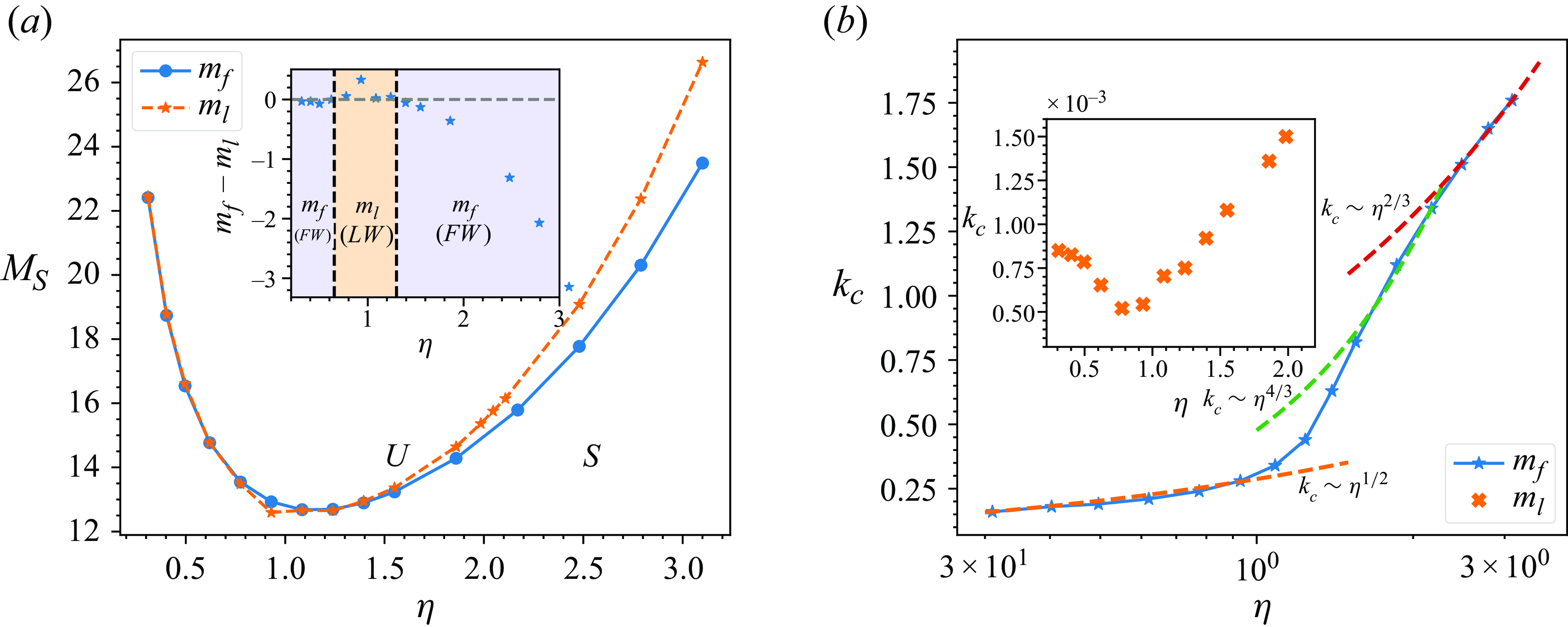
Figure 8. (a) Variation of the critical value of the solutal Marangoni number $M_S$
for a pure solutocapillary monotonic instability with the Soret coefficient
$M_S$
for a pure solutocapillary monotonic instability with the Soret coefficient $\eta$
in the case of cooling at the substrate
$\eta$
in the case of cooling at the substrate $\mathcal{Q}=-1$
with
$\mathcal{Q}=-1$
with $a=7.47,\,\Phi =0.01,\,L=10^{-3},\,M_T = 0,\,G=6.71,\,\Sigma _0=2\times 10^{4}$
and
$a=7.47,\,\Phi =0.01,\,L=10^{-3},\,M_T = 0,\,G=6.71,\,\Sigma _0=2\times 10^{4}$
and $B = 0.01$
; the inset shows the difference
$B = 0.01$
; the inset shows the difference $m_f-m_l$
between the two minimal values of
$m_f-m_l$
between the two minimal values of $M_S$
of the two solutocapillary modes versus
$M_S$
of the two solutocapillary modes versus $\eta$
. (b) Variation of the critical wavenumber
$\eta$
. (b) Variation of the critical wavenumber $k_c$
corresponding to the short-wave minimum
$k_c$
corresponding to the short-wave minimum $M_S=m_f$
with
$M_S=m_f$
with $\eta$
; the inset shows the variation of the wavenumber
$\eta$
; the inset shows the variation of the wavenumber $k$
corresponding to the long-wave mode
$k$
corresponding to the long-wave mode $M_S=m_l$
with
$M_S=m_l$
with $\eta$
. The dashed lines display various ranges of the data fit for the critical wavenumber as a function of
$\eta$
. The dashed lines display various ranges of the data fit for the critical wavenumber as a function of $\eta$
. The symbols
$\eta$
. The symbols $U$
and
$U$
and $S$
denote the unstable and stable domains of the system, respectively. FW and LW stand for domains of finite-wave and long-wave instability, respectively.
$S$
denote the unstable and stable domains of the system, respectively. FW and LW stand for domains of finite-wave and long-wave instability, respectively.
Figure 8(a) illustrates the non-monotonic variation of the critical solutal Marangoni number $M_S$
with the Soret coefficient
$M_S$
with the Soret coefficient $\eta$
for both competing modes. We find that the temperature difference across the layer of the base state given by
$\eta$
for both competing modes. We find that the temperature difference across the layer of the base state given by $\displaystyle \Delta T^*=q^*h_0^*/K_{bf}^*$
influences the value of the Soret coefficient
$\displaystyle \Delta T^*=q^*h_0^*/K_{bf}^*$
influences the value of the Soret coefficient $\eta$
defined in (2.17) and affects the competition between the long-wave deformational mode
$\eta$
defined in (2.17) and affects the competition between the long-wave deformational mode $M_S=m_l$
and the finite-wave pattern forming mode
$M_S=m_l$
and the finite-wave pattern forming mode $M_S=m_f$
. The inset of figure 8(a) displays the domains of instability versus the parameter
$M_S=m_f$
. The inset of figure 8(a) displays the domains of instability versus the parameter $\eta$
. We find that in the narrow range of the Soret coefficient
$\eta$
. We find that in the narrow range of the Soret coefficient $0.62 \leqslant \eta \leqslant 1.24$
corresponding to the temperature difference
$0.62 \leqslant \eta \leqslant 1.24$
corresponding to the temperature difference $2$
K
$2$
K $\leqslant \Delta T^\ast \leqslant 4$
K, the deformational mode
$\leqslant \Delta T^\ast \leqslant 4$
K, the deformational mode $M_S=m_l$
dominates over the finite-wave mode
$M_S=m_l$
dominates over the finite-wave mode $M_S=m_f$
in terms of the instability onset, namely
$M_S=m_f$
in terms of the instability onset, namely $m_l\lt m_f$
. Outside of this range of
$m_l\lt m_f$
. Outside of this range of $\eta$
, with a sufficiently low value of the modified Galileo number
$\eta$
, with a sufficiently low value of the modified Galileo number $G$
, the finite-wave mode
$G$
, the finite-wave mode $M_S=m_f$
prevails over the long-wave mode
$M_S=m_f$
prevails over the long-wave mode $M_S=m_l$
and determines the instability onset, namely
$M_S=m_l$
and determines the instability onset, namely $m_f\lt m_l$
. Figure 8(b) displays the variation of the critical wavenumber
$m_f\lt m_l$
. Figure 8(b) displays the variation of the critical wavenumber $k_c$
with the Soret coefficient
$k_c$
with the Soret coefficient $\eta$
. We observe that the critical wavenumber increases with
$\eta$
. We observe that the critical wavenumber increases with $\eta$
and exhibits three different functional variations with
$\eta$
and exhibits three different functional variations with $\eta$
. Notably, we observe that the critical wavenumber
$\eta$
. Notably, we observe that the critical wavenumber $k_c$
follows the scaling
$k_c$
follows the scaling $k_c \sim \eta ^{1/2}$
up to the value of
$k_c \sim \eta ^{1/2}$
up to the value of $\eta$
corresponding to the minimum of
$\eta$
corresponding to the minimum of $k_c$
for
$k_c$
for $M_S=m_l$
, which is shown in the inset of figure 8(a). This is followed by two different scalings
$M_S=m_l$
, which is shown in the inset of figure 8(a). This is followed by two different scalings $k_c \sim \eta ^{4/3}$
and
$k_c \sim \eta ^{4/3}$
and $k_c \sim \eta ^{2/3}$
for higher values of
$k_c \sim \eta ^{2/3}$
for higher values of $\eta$
. The inset of figure 8(b) also shows that the critical wavenumber for the long-wave mode
$\eta$
. The inset of figure 8(b) also shows that the critical wavenumber for the long-wave mode $M_S=m_l$
exhibits a non-monotonic variation with
$M_S=m_l$
exhibits a non-monotonic variation with $\eta$
in its relevant subdomain.
$\eta$
in its relevant subdomain.
Finally, we conclude that in the case of the layer cooled at the substrate, the pure solutocapillary instability is monotonic. It also remains monotonic when stabilising thermocapillarity is present along with gravity, the Soret effect and interfacial deformation. The type of this instability is finite-wave for both sufficiently low and sufficiently high values of the modified Galileo number $G$
, whereas in the intermediate range of
$G$
, whereas in the intermediate range of $G$
, it is long-wave. A similar feature takes place with a variation of the Soret coefficient
$G$
, it is long-wave. A similar feature takes place with a variation of the Soret coefficient $\eta$
. Last, but not least, the fact that only the monotonic solutocapillary instability emerges in the case of cooling at the substrate is similar to what Sarma & Mondal (Reference Sarma and Mondal2021b
) found in this case making a statement that the monotonic mode is independent of the degree of viscoelasticity of the binary fluid. However, in contrast with the results obtained by Sarma & Mondal (Reference Sarma and Mondal2021b
) pointing to the emergence of the long-wave instability, our results show that the emerging solutocapillary instability may be either long-wave or finite-wave depending on the system parameters. This difference in the results between the current paper and Sarma & Mondal (Reference Sarma and Mondal2021b
) is possibly due to the presence of concentration-dependent thermophysical properties of the nanofluid.
$\eta$
. Last, but not least, the fact that only the monotonic solutocapillary instability emerges in the case of cooling at the substrate is similar to what Sarma & Mondal (Reference Sarma and Mondal2021b
) found in this case making a statement that the monotonic mode is independent of the degree of viscoelasticity of the binary fluid. However, in contrast with the results obtained by Sarma & Mondal (Reference Sarma and Mondal2021b
) pointing to the emergence of the long-wave instability, our results show that the emerging solutocapillary instability may be either long-wave or finite-wave depending on the system parameters. This difference in the results between the current paper and Sarma & Mondal (Reference Sarma and Mondal2021b
) is possibly due to the presence of concentration-dependent thermophysical properties of the nanofluid.
4.3. Heating at the substrate
$(\mathcal{Q} = 1)$

In this section, we investigate the onset of instability in the case of a heated substrate and reveal that it may be either monotonic or oscillatory. Joo (Reference Joo1995) and Oron & Nepomnyashchy (Reference Oron and Nepomnyashchy2004) found that in the case of a layer of a dilute binary mixture with either deformable or non-deformable interface, the system exhibits competition between destabilising thermocapillarity and stabilising solutocapillarity, and as a result, the oscillatory instability emerges.
In the case of a nanofluid layer heated from below, the base state displays a profile of the particle concentration increasing with height. Therefore, if the particle density is higher than that of the liquid, then, in the presence of gravity, there exists an ingredient of Rayleigh–Taylor instability (Chandrasekhar Reference Chandrasekhar1961), which, in what follows, will be referred to as a solutal buoyancy due to its qualitative similarity to the thermal buoyancy.
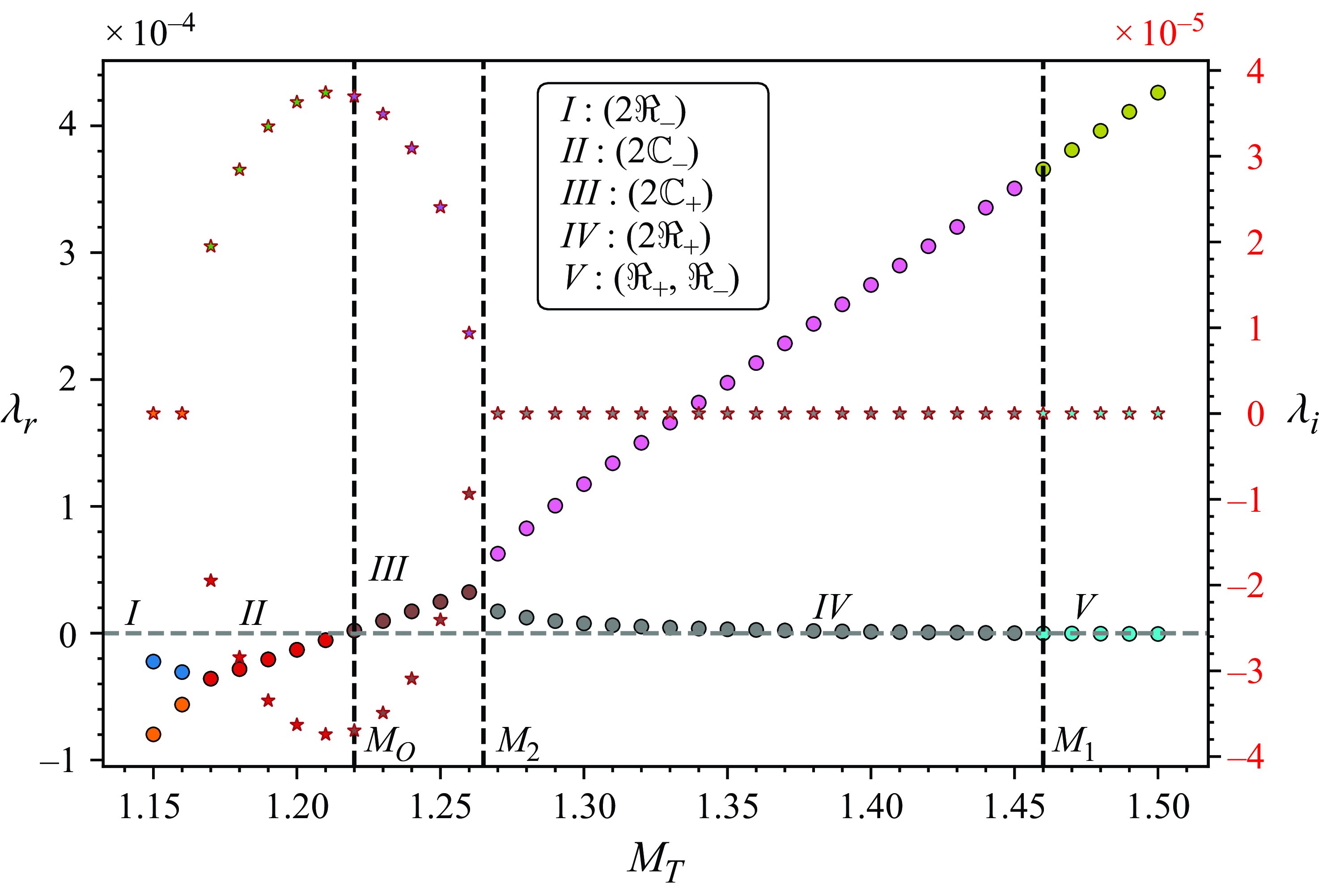
Figure 9. Eigenspectrum map of the two leading eigenvalues $\lambda$
in the complex plane spanned by their growth rate (the real part
$\lambda$
in the complex plane spanned by their growth rate (the real part $\Re (\lambda ) \equiv \lambda _r$
the vertical axis on the left) and their frequency (the imaginary part
$\Re (\lambda ) \equiv \lambda _r$
the vertical axis on the left) and their frequency (the imaginary part $\Im (\lambda ) \equiv \lambda _i$
– the vertical axis on the right) versus
$\Im (\lambda ) \equiv \lambda _i$
– the vertical axis on the right) versus $M_T$
in the case of heating at the substrate
$M_T$
in the case of heating at the substrate $\mathcal{Q}=1$
with
$\mathcal{Q}=1$
with $\Phi =0.01,$ $G=1,$ $\Sigma _0=10,$ $\eta =0.31,$ $L=10^{-3},$ $a=7.47,$ $M_S=0,$ $P=7,$ $B=0.01$
and
$B=0.01$
and $k=0.18$
. The domains
$k=0.18$
. The domains $I{-}V$
are the domains with two negative real eigenvalues (
$I{-}V$
are the domains with two negative real eigenvalues ( $2\Re _-$
), two complex conjugate eigenvalues with a negative real part (
$2\Re _-$
), two complex conjugate eigenvalues with a negative real part ( $2\mathbb{C}_-$
), two complex conjugate eigenvalues with a positive real part (
$2\mathbb{C}_-$
), two complex conjugate eigenvalues with a positive real part ( $2\mathbb{C}_+$
), two positive real eigenvalues (
$2\mathbb{C}_+$
), two positive real eigenvalues ( $2\Re _+$
), and two real eigenvalues (one positive (
$2\Re _+$
), and two real eigenvalues (one positive ( $\Re _+$
) and one negative (
$\Re _+$
) and one negative ( $\Re _-$
) ), respectively. The circle
$\Re _-$
) ), respectively. The circle $(\circ )$
and star
$(\circ )$
and star $(\star )$
points correspond to the real and imaginary parts of the complex growth rate
$(\star )$
points correspond to the real and imaginary parts of the complex growth rate $\lambda$
, respectively. The vertical dashed lines represent the transition from the subdomain
$\lambda$
, respectively. The vertical dashed lines represent the transition from the subdomain $II$
to the subdomain
$II$
to the subdomain $III$
, from
$III$
, from $III$
to
$III$
to $IV$
and from
$IV$
and from $IV$
to
$IV$
to $V$
. The horizontal dashed line represents
$V$
. The horizontal dashed line represents $\lambda _r=0$
.
$\lambda _r=0$
.
Figure 9 presents a typical example of the structure of the eigenspectrum of the problem given by (3.7) by following the two leading eigenvalue branches by increasing the thermal Marangoni number $M_T$
for
$M_T$
for $G=1$
near the critical wavenumber
$G=1$
near the critical wavenumber $k_c \approx 0.18$
for a parameter set specified in the caption. The entire variation range of
$k_c \approx 0.18$
for a parameter set specified in the caption. The entire variation range of $M_T$
is naturally subdivided into five different subdomains. With an increase in
$M_T$
is naturally subdivided into five different subdomains. With an increase in $M_T$
, the first subdomain (subdomain
$M_T$
, the first subdomain (subdomain $I$
) is where the two tracked eigenvalues are real and negative. The two branches of subdomain
$I$
) is where the two tracked eigenvalues are real and negative. The two branches of subdomain $I$
merge with an increase in
$I$
merge with an increase in $M_T$
and split into two branches, along which the eigenvalues are complex conjugate with the negative real part
$M_T$
and split into two branches, along which the eigenvalues are complex conjugate with the negative real part $\lambda _r$
; this is subdomain
$\lambda _r$
; this is subdomain $II$
. A combination of subdomains
$II$
. A combination of subdomains $I$
and
$I$
and $II$
belongs to the stability domain of the system. Following the two branches in the subdomain
$II$
belongs to the stability domain of the system. Following the two branches in the subdomain $II$
in figure 9, we observe that with an increase in
$II$
in figure 9, we observe that with an increase in $M_T$
, the frequency
$M_T$
, the frequency $\lambda _i$
of the two leading eigenvalues increases in its absolute value, whereas the growth rate
$\lambda _i$
of the two leading eigenvalues increases in its absolute value, whereas the growth rate $\lambda _r$
increases and crosses zero. We emphasise that the oscillatory instability emerges here in the case of
$\lambda _r$
increases and crosses zero. We emphasise that the oscillatory instability emerges here in the case of $M_S=0$
; hence, solutocapillarity is irrelevant. This is where the subdomain
$M_S=0$
; hence, solutocapillarity is irrelevant. This is where the subdomain $II$
ends and the subdomain
$II$
ends and the subdomain $III$
begins. In the subdomain
$III$
begins. In the subdomain $III$
, the two leading eigenvalues are still complex conjugates, but their real part
$III$
, the two leading eigenvalues are still complex conjugates, but their real part $\lambda _r$
is positive and, therefore, the system undergoes oscillatory instability. In the subdomain
$\lambda _r$
is positive and, therefore, the system undergoes oscillatory instability. In the subdomain $III$
, the growth rate
$III$
, the growth rate $\lambda _i$
increases with
$\lambda _i$
increases with $M_T$
, whereas the absolute value of the frequency
$M_T$
, whereas the absolute value of the frequency $|\lambda _i|$
decreases until it reaches its zero value, and the two leading eigenvalues become real and positive. At this point, the subdomain
$|\lambda _i|$
decreases until it reaches its zero value, and the two leading eigenvalues become real and positive. At this point, the subdomain $III$
ends at
$III$
ends at $M_T=M_2$
and the subdomain
$M_T=M_2$
and the subdomain $IV$
begins. In the subdomain
$IV$
begins. In the subdomain $IV$
, there are two real positive eigenvalues, one of them increases with an increase in
$IV$
, there are two real positive eigenvalues, one of them increases with an increase in $M_T$
, whereas the other one decreases until it reaches zero, where the subdomain
$M_T$
, whereas the other one decreases until it reaches zero, where the subdomain $IV$
ends at
$IV$
ends at $M_T=M_1$
, and the subdomain
$M_T=M_1$
, and the subdomain $V$
begins. In the subdomain
$V$
begins. In the subdomain $V$
, there is only one positive eigenvalue and the second leading eigenvalue is negative.
$V$
, there is only one positive eigenvalue and the second leading eigenvalue is negative.
As an illustration for figure 9, figure 10 presents the neutral curves $M_T(k)$
in the case of a moderately low Galileo number
$M_T(k)$
in the case of a moderately low Galileo number $G,\,G=1$
, and the parameter set of figure 9, where the pure thermocapillary oscillatory instability sets in at a finite wavenumber
$G,\,G=1$
, and the parameter set of figure 9, where the pure thermocapillary oscillatory instability sets in at a finite wavenumber $k \approx 0.18$
. Along with the neutral curve
$k \approx 0.18$
. Along with the neutral curve $M_T(k)$
, we present in figure 10 two more boundary curves that illustrate important features of the spectrum of the eigenvalue problem (3.7). The boundary located just above the threshold of the oscillatory instability in figure 10 marked as
$M_T(k)$
, we present in figure 10 two more boundary curves that illustrate important features of the spectrum of the eigenvalue problem (3.7). The boundary located just above the threshold of the oscillatory instability in figure 10 marked as $M_2$
separates the domain where two complex conjugate eigenvalues with a positive real part exist from the domain of two real leading positive eigenvalues. The space between the
$M_2$
separates the domain where two complex conjugate eigenvalues with a positive real part exist from the domain of two real leading positive eigenvalues. The space between the $M_O$
and
$M_O$
and $M_2$
lines constitutes the subdomain
$M_2$
lines constitutes the subdomain $III$
. Slightly further above the boundary
$III$
. Slightly further above the boundary $M_2$
lies one more boundary marked as
$M_2$
lies one more boundary marked as $M_1$
along which one of the leading positive eigenvalues turns to be zero, whereas the other one remains positive. The emergence of several boundaries in a close proximity illustrates a competition between thermocapillarity, gravity and other factors such as the Soret effect, interfacial deformability and possibly concentration-dependence of the thermal conductivity of the suspension which will be discussed below.
$M_1$
along which one of the leading positive eigenvalues turns to be zero, whereas the other one remains positive. The emergence of several boundaries in a close proximity illustrates a competition between thermocapillarity, gravity and other factors such as the Soret effect, interfacial deformability and possibly concentration-dependence of the thermal conductivity of the suspension which will be discussed below.
Figure 10. Pure thermocapillary oscillatory instability for the case of heating at the substrate $\mathcal{Q}=1$
and the parameter set of figure 9. The lowest curve marked as
$\mathcal{Q}=1$
and the parameter set of figure 9. The lowest curve marked as $M_O$
represents the onset of instability
$M_O$
represents the onset of instability $M_T(k)$
showing the thermal Marangoni number versus the wavenumber
$M_T(k)$
showing the thermal Marangoni number versus the wavenumber $k$
. The subdomains
$k$
. The subdomains $I {-} V$
correspond to the respective subdomains in figure 9.
$I {-} V$
correspond to the respective subdomains in figure 9. $M_1$
,
$M_1$
, $M_2$
and
$M_2$
and $M_O$
are transition values of
$M_O$
are transition values of $M_T$
between domains
$M_T$
between domains $IV$
to
$IV$
to $V$
, from
$V$
, from $III$
to
$III$
to $IV$
and from
$IV$
and from $II$
to
$II$
to $III$
, respectively.
$III$
, respectively.
The branch of the larger real eigenvalue in the subdomains $IV$
and
$IV$
and $V$
corresponds to the thermocapillary mode which increases almost linearly with an increase in the Marangoni number
$V$
corresponds to the thermocapillary mode which increases almost linearly with an increase in the Marangoni number $M_T$
. The branch of the smaller real eigenvalue, which remains positive but very small in the domain
$M_T$
. The branch of the smaller real eigenvalue, which remains positive but very small in the domain $IV$
and crossing zero at
$IV$
and crossing zero at $M=M_1$
, is driven by particle diffusion, which is coupled with the unstable thermal mode. To check this observation, we have increased the Lewis number
$M=M_1$
, is driven by particle diffusion, which is coupled with the unstable thermal mode. To check this observation, we have increased the Lewis number $L$
ten-fold, thereby effectively leading to a ten-fold increase in the smaller eigenvalue and, as a result of this, the positive decreasing branch of the second leading eigenvalue has decayed much faster and, therefore,
$L$
ten-fold, thereby effectively leading to a ten-fold increase in the smaller eigenvalue and, as a result of this, the positive decreasing branch of the second leading eigenvalue has decayed much faster and, therefore, $M_1$
has decreased. It turns out that the same decreasing branch weakly depends on the surface tension number
$M_1$
has decreased. It turns out that the same decreasing branch weakly depends on the surface tension number $\Sigma _0$
as well.
$\Sigma _0$
as well.
Figure 11. Pure thermocapillary instability in the case of heating at the substrate $\mathcal{Q}=1$
with
$\mathcal{Q}=1$
with $\Phi =0.01,$ $\Sigma _0=10,$ $\eta =0.31,$ $L=10^{-3},$ $B=0.01,$ $M_S=0,$ $P=7.$
(a) Variation of the instability threshold
$P=7.$
(a) Variation of the instability threshold $M_T$
with the modified Galileo number
$M_T$
with the modified Galileo number $G$
. The circle
$G$
. The circle $(\circ )$
and star
$(\circ )$
and star $(\star )$
points correspond to the monotonic and oscillatory modes, respectively; inset shows the upper line
$(\star )$
points correspond to the monotonic and oscillatory modes, respectively; inset shows the upper line $M_T(G)$
above which the long-wave mode becomes unstable. Note that these values of
$M_T(G)$
above which the long-wave mode becomes unstable. Note that these values of $M_T$
are much larger than the critical values of
$M_T$
are much larger than the critical values of $M_T$
for the oscillatory instability for
$M_T$
for the oscillatory instability for $G \lt 55.6$
, so the values of the latter appear as zero. However, for
$G \lt 55.6$
, so the values of the latter appear as zero. However, for $G \geqslant 55.6$
, the solutal buoyancy becomes dominant and drives the long-wave solutal buoyancy monotonic instability with the critical Marangoni number
$G \geqslant 55.6$
, the solutal buoyancy becomes dominant and drives the long-wave solutal buoyancy monotonic instability with the critical Marangoni number $M_T=0$
and the critical wavenumber
$M_T=0$
and the critical wavenumber $k_c=0$
. (b) Variation of the growth rate
$k_c=0$
. (b) Variation of the growth rate $\lambda$
versus wavenumber
$\lambda$
versus wavenumber $k$
for
$k$
for $M_T=0$
for several values of
$M_T=0$
for several values of $G$
in the domain of solutal buoyancy instability,
$G$
in the domain of solutal buoyancy instability, $G \gt 55.6$
. The dashed lines illustrate data fit proportional to
$G \gt 55.6$
. The dashed lines illustrate data fit proportional to $k^2$
with the proportionality coefficient increasing with
$k^2$
with the proportionality coefficient increasing with $G$
. The symbols
$G$
. The symbols $U,\,U^\dagger, $
and
$U,\,U^\dagger, $
and $S$
represent the domains where the two leading eigenvalues are real and positive, complex conjugates with a positive real part and complex conjugates with a negative real part, respectively.
$S$
represent the domains where the two leading eigenvalues are real and positive, complex conjugates with a positive real part and complex conjugates with a negative real part, respectively.
Based on our earlier discussion, it is essential to understand the role of gravity in the onset of instability of the system at hand. Figure 11(a) displays the variation of the critical value of the thermal Marangoni number $M_T$
with the modified Galileo number
$M_T$
with the modified Galileo number $G$
in the case of a pure thermocapillary instability. Here, we note that for sufficiently low values of
$G$
in the case of a pure thermocapillary instability. Here, we note that for sufficiently low values of $G$
, the monotonic instability sets in. Note the difference with the case of
$G$
, the monotonic instability sets in. Note the difference with the case of $G=1$
presented in figures 9 and 10, where the oscillatory instability takes place. Following the monotonic branch of the
$G=1$
presented in figures 9 and 10, where the oscillatory instability takes place. Following the monotonic branch of the $M_T{-}G$
plane, we observe that at
$M_T{-}G$
plane, we observe that at $G \approx 10^{-1}$
, the monotonic branch becomes the
$G \approx 10^{-1}$
, the monotonic branch becomes the $M_1$
- branch presented in figures 9 and 10 for
$M_1$
- branch presented in figures 9 and 10 for $G=1$
, and the system undergoes the oscillatory instability. The left vertical dashed line in figure 11(a) represents the asymptotic line for the monotonic branch
$G=1$
, and the system undergoes the oscillatory instability. The left vertical dashed line in figure 11(a) represents the asymptotic line for the monotonic branch $\lambda =0$
. Note the
$\lambda =0$
. Note the $M_2$
branch is not presented here to not overburden the figure. Also, there exists a branch above which the long-wave mode becomes unstable (shown in the inset). However, since the values of
$M_2$
branch is not presented here to not overburden the figure. Also, there exists a branch above which the long-wave mode becomes unstable (shown in the inset). However, since the values of $M_T$
along this branch are much higher than those along the monotonic and oscillatory branches discussed above, it is irrelevant for the onset of instability.
$M_T$
along this branch are much higher than those along the monotonic and oscillatory branches discussed above, it is irrelevant for the onset of instability.
As mentioned above, in the case of heating at the substrate considered now, the density stratification in the layer is unstable for particles heavier than the carrier fluid, e.g., $\rho _{np}=4$
, and, in addition to the Marangoni effect, there exists at least one more instability ingredient referred to as solutal buoyancy. Also, gravity plays both stabilising and destabilising roles in the long-wavelength range, i.e. an increase in
$\rho _{np}=4$
, and, in addition to the Marangoni effect, there exists at least one more instability ingredient referred to as solutal buoyancy. Also, gravity plays both stabilising and destabilising roles in the long-wavelength range, i.e. an increase in $G$
may promote the solutal buoyancy instability, but at the same time, the deformable interface tends to flatten out and to relieve a tendency to instability. We note that for relatively low values of
$G$
may promote the solutal buoyancy instability, but at the same time, the deformable interface tends to flatten out and to relieve a tendency to instability. We note that for relatively low values of $G$
, the solutal buoyancy mechanism is weak and the monotonic thermocapillary instability dominates. However, we find that with an increase in the value of
$G$
, the solutal buoyancy mechanism is weak and the monotonic thermocapillary instability dominates. However, we find that with an increase in the value of $G$
, the solutal buoyancy mechanism becomes stronger, and, at a sufficiently large value of
$G$
, the solutal buoyancy mechanism becomes stronger, and, at a sufficiently large value of $G$
,
$G$
, $G \approx 55.6$
(marked by the right vertical dashed line shown also in the inset) for the given parameter set, it dominates over both the oscillatory thermocapillary instability and a long-wave solutal buoyancy instability emerging at
$G \approx 55.6$
(marked by the right vertical dashed line shown also in the inset) for the given parameter set, it dominates over both the oscillatory thermocapillary instability and a long-wave solutal buoyancy instability emerging at $M_T=0$
marked by a horizontal thick line for
$M_T=0$
marked by a horizontal thick line for $G \geqslant 55.6$
with the critical wavenumber
$G \geqslant 55.6$
with the critical wavenumber $k_c=0$
. Figure 11(b) illustrates the growth rate
$k_c=0$
. Figure 11(b) illustrates the growth rate $\lambda$
variation for different values of
$\lambda$
variation for different values of $G,\, G\gt 55.6$
with the data fit proportional to
$G,\, G\gt 55.6$
with the data fit proportional to $k^2$
for
$k^2$
for $M_T=0$
. We also find that the proportionality constant increases with the value of
$M_T=0$
. We also find that the proportionality constant increases with the value of $G$
within the unstable domain. As expected, the range of instability widens with an increase in
$G$
within the unstable domain. As expected, the range of instability widens with an increase in $G$
.
$G$
.
Figure 12. Pure thermocapillary stability boundaries versus wavenumber $k$
in the domain of solutal buoyancy instability for the case of heating at the substrate
$k$
in the domain of solutal buoyancy instability for the case of heating at the substrate $\mathcal{Q}=1$
with
$\mathcal{Q}=1$
with $\Phi =0.01,$ $\Sigma _0=10,$ $\eta =0.31,$ $L=10^{-3},$ $M_S=0,$ $a=7.47,$ $P=7$
and
$P=7$
and $B=0.01$
. The two solid (blue) curves on the left and the solid (red) curve on the right represent the monotonic and oscillatory boundaries with the vertical axes on the left and right vertical axes, respectively, for the two values of
$B=0.01$
. The two solid (blue) curves on the left and the solid (red) curve on the right represent the monotonic and oscillatory boundaries with the vertical axes on the left and right vertical axes, respectively, for the two values of $G, G=55.8$
and
$G, G=55.8$
and $G=56$
. Note that, unlike the curves for the monotonic instability, the curves for the oscillatory instability almost overlap. Straight dashed lines represent the data fit
$G=56$
. Note that, unlike the curves for the monotonic instability, the curves for the oscillatory instability almost overlap. Straight dashed lines represent the data fit $M_T \sim \alpha k^{-\beta }$
with
$M_T \sim \alpha k^{-\beta }$
with $(\alpha =5.77\times 10^{-5}, \beta =2.2)$
for
$(\alpha =5.77\times 10^{-5}, \beta =2.2)$
for $G=55.8$
and
$G=55.8$
and $(\alpha =1.91\times 10^{-4}, \beta =2.12)$
for
$(\alpha =1.91\times 10^{-4}, \beta =2.12)$
for $G=56$
. The symbols
$G=56$
. The symbols $U,\,U^\dagger, $
and
$U,\,U^\dagger, $
and $S$
represent the domains of monotonic solutal buoyancy instability, of two complex conjugate leading eigenvalues with a positive real part, and that of stability, respectively.
$S$
represent the domains of monotonic solutal buoyancy instability, of two complex conjugate leading eigenvalues with a positive real part, and that of stability, respectively.
Figure 12 presents more details related to the structure of the eigenspectrum of the system for the parameter set used in figure 11 in the range of $G$
adjacent to the onset of the solutal buoyancy instability. We observe that the long-wave monotonic branch
$G$
adjacent to the onset of the solutal buoyancy instability. We observe that the long-wave monotonic branch $\lambda =0$
of the thermocapillary mode crosses zero at a finite but small wavenumber
$\lambda =0$
of the thermocapillary mode crosses zero at a finite but small wavenumber $k_c$
shown in figure 11(b). These curves represent boundaries of stabilisation of the thermocapillarity where the domain of instability and stability of the system are located beneath and above the corresponding curve. Therefore, higher values of
$k_c$
shown in figure 11(b). These curves represent boundaries of stabilisation of the thermocapillarity where the domain of instability and stability of the system are located beneath and above the corresponding curve. Therefore, higher values of $M_T$
stabilise the system. The instability range of the system in the solutal buoyancy regime expands with an increase in
$M_T$
stabilise the system. The instability range of the system in the solutal buoyancy regime expands with an increase in $G$
in terms of
$G$
in terms of $M_T$
and
$M_T$
and $k_c$
. In the same range of
$k_c$
. In the same range of $G$
, we also find that the oscillatory branch shown in the inset of figure 11(a) continues further into the solutal buoyancy domain, as also shown in figure 12 with the corresponding scale on the right-hand side of the figure. It is noted that the values of
$G$
, we also find that the oscillatory branch shown in the inset of figure 11(a) continues further into the solutal buoyancy domain, as also shown in figure 12 with the corresponding scale on the right-hand side of the figure. It is noted that the values of $M_T$
along the oscillatory finite-wave branch are much higher than those along the monotonic branches. Hence, in the range of finite wavenumbers
$M_T$
along the oscillatory finite-wave branch are much higher than those along the monotonic branches. Hence, in the range of finite wavenumbers $k$
, the oscillatory mode emerges in the solutal buoyancy instability domain and, within the range of the wavenumbers corresponding to this instability, the long-wave instability does not set in.
$k$
, the oscillatory mode emerges in the solutal buoyancy instability domain and, within the range of the wavenumbers corresponding to this instability, the long-wave instability does not set in.
The variation of the critical wavenumber $k_c$
along the instability curves
$k_c$
along the instability curves $M_T(G)$
shown in figure 11(a), are displayed in figure 13(a). We note that the critical wavenumber
$M_T(G)$
shown in figure 11(a), are displayed in figure 13(a). We note that the critical wavenumber $k_c$
increases monotonically with
$k_c$
increases monotonically with $G$
along both the monotonic and oscillatory instability thresholds. Also, along the stretch of the monotonic mode when it does not represent the instability onset, the minimal wavenumber is lower than the critical wavenumber
$G$
along both the monotonic and oscillatory instability thresholds. Also, along the stretch of the monotonic mode when it does not represent the instability onset, the minimal wavenumber is lower than the critical wavenumber $k_c$
. In addition, we find that the critical wavenumber
$k_c$
. In addition, we find that the critical wavenumber $k_c$
along the monotonic stabilisation boundary tends to zero with an increase in
$k_c$
along the monotonic stabilisation boundary tends to zero with an increase in $G$
. Figure 13(b) displays a non-monotonic variation of the growth rate
$G$
. Figure 13(b) displays a non-monotonic variation of the growth rate $\lambda$
with
$\lambda$
with $k$
for several values of
$k$
for several values of $G$
near the onset of the solutal buoyancy instability. Figure 13(c) shows the monotonic increase in the critical frequency along the oscillatory branch presented in figure 13(a) with the modified Galileo number
$G$
near the onset of the solutal buoyancy instability. Figure 13(c) shows the monotonic increase in the critical frequency along the oscillatory branch presented in figure 13(a) with the modified Galileo number $G$
.
$G$
.
Figure 13. Pure thermocapillary instability in the case of heating at the substrate $\mathcal{Q}=1$
with
$\mathcal{Q}=1$
with $\Phi =0.01,$ $\eta =0.31,$ $L=10^{-3},$ $a=7.47,$ $\Sigma _0=10,$ $M_S=0,$ $B=0.01$
. (a) Variation of the critical wavenumber
$B=0.01$
. (a) Variation of the critical wavenumber $k_c$
versus the modified Galileo number
$k_c$
versus the modified Galileo number $G$
. The
$G$
. The $\circ$
,
$\circ$
, $\star$
and
$\star$
and $\times$
points in the inset represent the critical wavenumber
$\times$
points in the inset represent the critical wavenumber $k_c$
for the monotonic, oscillatory and solutal buoyancy instability, respectively. Inset shows the variation of the minimal wavenumber
$k_c$
for the monotonic, oscillatory and solutal buoyancy instability, respectively. Inset shows the variation of the minimal wavenumber $k$
in the long-wave mode versus
$k$
in the long-wave mode versus $G$
in the transition domain,
$G$
in the transition domain, $55 \leqslant G \leqslant 56.5$
. (b) Variation of the growth rate
$55 \leqslant G \leqslant 56.5$
. (b) Variation of the growth rate $\lambda$
versus wavenumber
$\lambda$
versus wavenumber $k$
in the transition domain for various
$k$
in the transition domain for various $G$
. (c) Variation of the frequency
$G$
. (c) Variation of the frequency $\lambda _i$
versus the modified Galileo number
$\lambda _i$
versus the modified Galileo number $G$
along the oscillatory instability threshold of panel (a).
$G$
along the oscillatory instability threshold of panel (a).
Figure 14(a) shows the neutral curves in the case of a pure thermocapillary monotonic instability for a small Galileo number $G=0.01$
for different Biot numbers
$G=0.01$
for different Biot numbers $B$
. The results for the instability threshold shown in the
$B$
. The results for the instability threshold shown in the $M_T{-}G$
plane in figure 11(a) suggest that the parameter set here for
$M_T{-}G$
plane in figure 11(a) suggest that the parameter set here for $B=0.01$
corresponds to the monotonic instability. The instability remains monotonic for the two other values of the Biot number
$B=0.01$
corresponds to the monotonic instability. The instability remains monotonic for the two other values of the Biot number $B$
. As in the case of the Marangoni instability in a simple fluid (Pearson Reference Pearson1958), we find that the stability domain located underneath the neutral curves expands with an increase in the Biot number accompanied with an increase of the critical Marangoni number
$B$
. As in the case of the Marangoni instability in a simple fluid (Pearson Reference Pearson1958), we find that the stability domain located underneath the neutral curves expands with an increase in the Biot number accompanied with an increase of the critical Marangoni number $M_T$
at the minimum of the corresponding neutral curve. This is due to the fact that a higher Biot number implies that the system loses some of the heat to the atmosphere, and therefore it requires a higher temperature drop or the heat flux transferred into the system, equivalently, a higher
$M_T$
at the minimum of the corresponding neutral curve. This is due to the fact that a higher Biot number implies that the system loses some of the heat to the atmosphere, and therefore it requires a higher temperature drop or the heat flux transferred into the system, equivalently, a higher $M_T$
to drive the Marangoni instability (Davis Reference Davis1987). Further, figure 14(b) presents the variation of the critical wavenumber
$M_T$
to drive the Marangoni instability (Davis Reference Davis1987). Further, figure 14(b) presents the variation of the critical wavenumber $k_c$
with the Biot number
$k_c$
with the Biot number $B$
. It follows the relationship
$B$
. It follows the relationship $k_c \sim B^{1/4}$
which is a known asymptotic limit for the Marangoni instability in a simple Newtonian fluid (Sivashinsky Reference Sivashinsky1982) and is also one of the two known asymptotic limits for the long-wave instability in dilute binary fluids (Podolny et al. Reference Podolny, Oron and Nepomnyashchy2005) in the limit of small Biot numbers.
$k_c \sim B^{1/4}$
which is a known asymptotic limit for the Marangoni instability in a simple Newtonian fluid (Sivashinsky Reference Sivashinsky1982) and is also one of the two known asymptotic limits for the long-wave instability in dilute binary fluids (Podolny et al. Reference Podolny, Oron and Nepomnyashchy2005) in the limit of small Biot numbers.
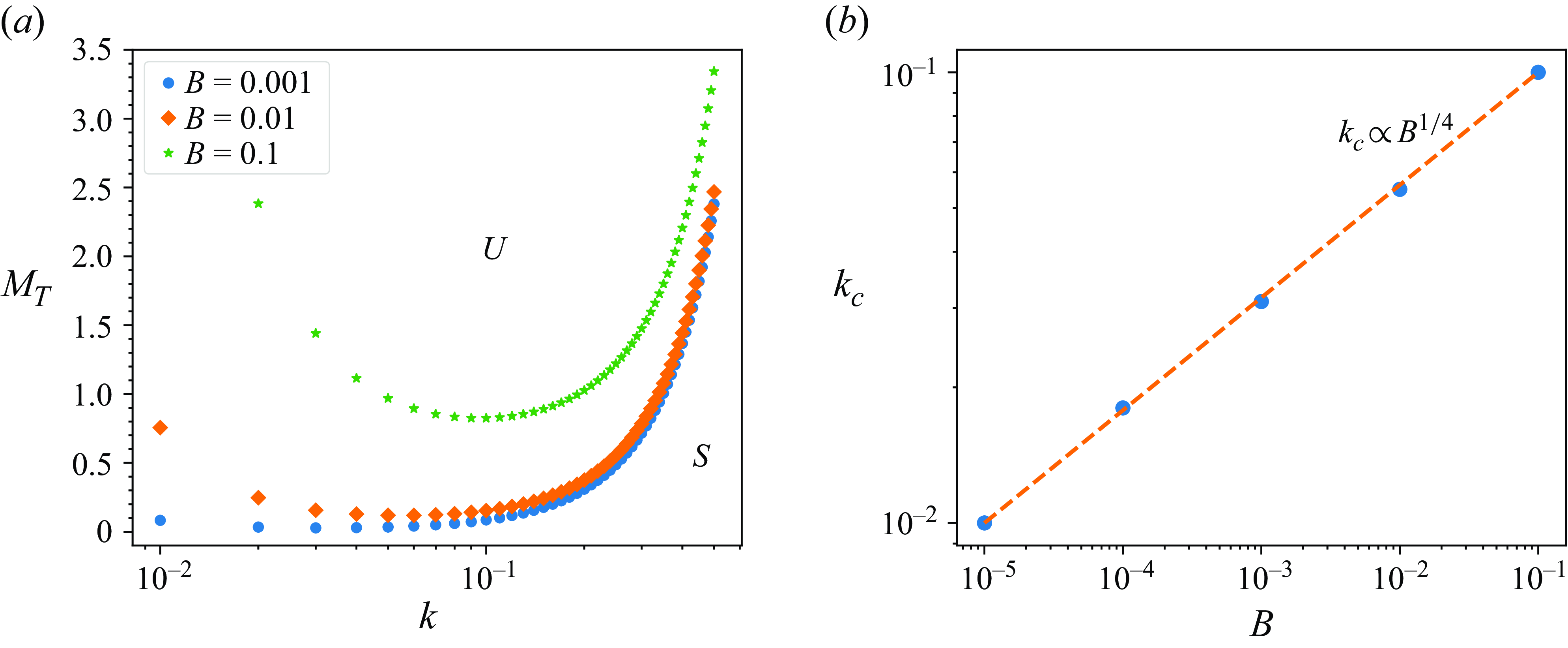
Figure 14. Pure monotonic thermocapillary instability in the case of heating at the substrate $\mathcal{Q}=1$
at
$\mathcal{Q}=1$
at $\Phi =0.01,$ $\eta =0.31,$ $L=10^{-3},$ $a=7.47,$ $M_S = 0,$ $\Sigma _0=10,$ $G=0.01$
. (a) Neutral curves
$G=0.01$
. (a) Neutral curves $M_T(k)$
for various Biot numbers
$M_T(k)$
for various Biot numbers $B$
. The symbols
$B$
. The symbols $U$
and
$U$
and $S$
denote the unstable and stable domains, respectively. (b) Variation of the critical wavenumber
$S$
denote the unstable and stable domains, respectively. (b) Variation of the critical wavenumber $k_c$
with the Biot number
$k_c$
with the Biot number $B$
. The dashed line represents the data fit
$B$
. The dashed line represents the data fit $k_c \sim B^{1/4}$
with the factor of
$k_c \sim B^{1/4}$
with the factor of $0.178$
. The filled circle points correspond to the numerical solution of the EVP, (3.7).
$0.178$
. The filled circle points correspond to the numerical solution of the EVP, (3.7).
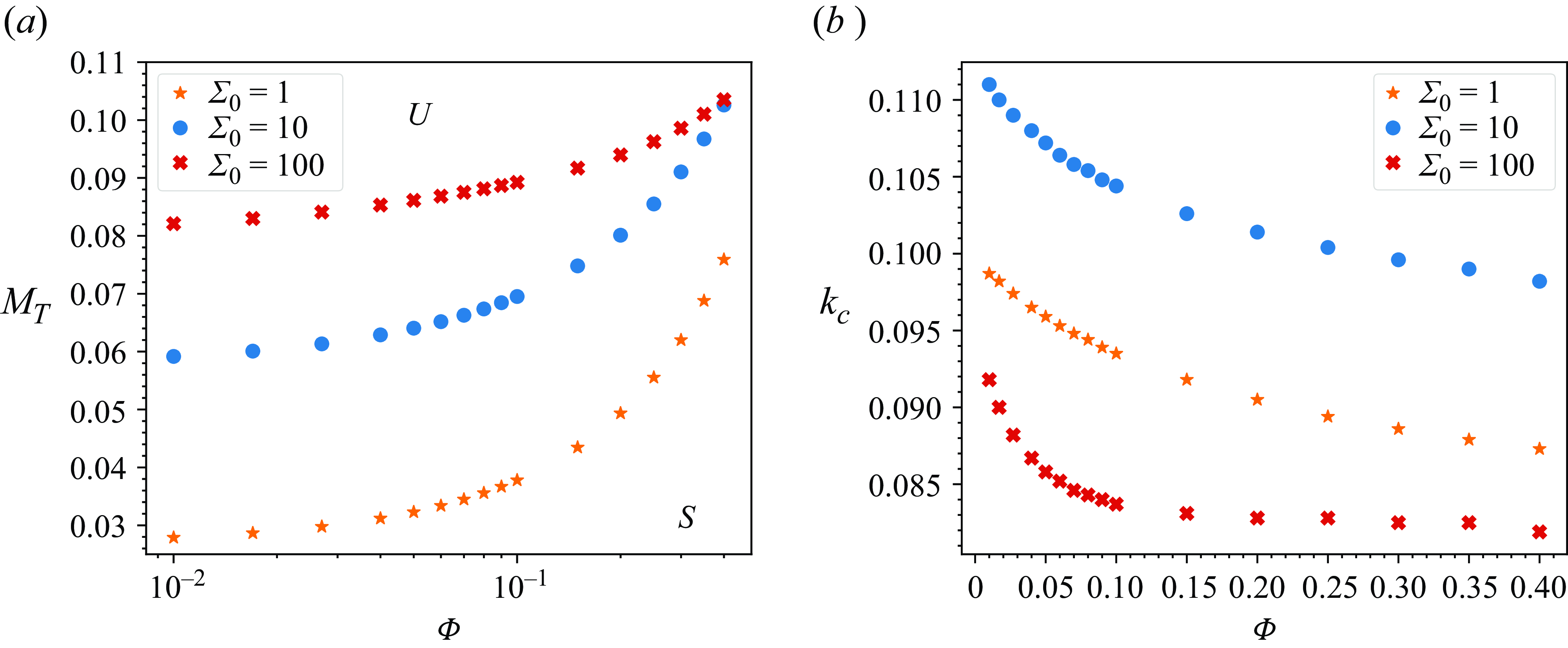
Figure 15. Pure monotonic thermocapillary instability in the case of heating at the substrate $\mathcal{Q}=1$
at
$\mathcal{Q}=1$
at $B=0.01,$ $\eta =0.31,$ $L=10^{-3},$ $a=7.47,$ $M_S = 0$
and
$M_S = 0$
and $G=0.01$
for several values of the inverse capillary number
$G=0.01$
for several values of the inverse capillary number $\Sigma _0$
. (a) Variation of the critical thermal Marangoni number
$\Sigma _0$
. (a) Variation of the critical thermal Marangoni number $M_T$
with the averaged bulk nanoparticle concentration
$M_T$
with the averaged bulk nanoparticle concentration $\Phi$
, where
$\Phi$
, where $ M_T/2$
and
$ M_T/2$
and $M_T/10$
are presented for
$M_T/10$
are presented for $\Sigma _0=10$
and
$\Sigma _0=10$
and $\Sigma _0=100$
, respectively. The symbols
$\Sigma _0=100$
, respectively. The symbols $U$
and
$U$
and $S$
denote the unstable and stable domains of the system, respectively. (b) Variation of the critical wavenumber
$S$
denote the unstable and stable domains of the system, respectively. (b) Variation of the critical wavenumber $k_c$
with
$k_c$
with $\Phi$
, where
$\Phi$
, where $2 k_c$
and
$2 k_c$
and $3 k_c$
are presented for
$3 k_c$
are presented for $\Sigma _0=10$
and
$\Sigma _0=10$
and $\Sigma _0=100$
, respectively.
$\Sigma _0=100$
, respectively.
Figure 15(a) presents the variation of the critical thermal Marangoni number $M_T$
with the mean particle concentration
$M_T$
with the mean particle concentration $\Phi$
. We note that the latter directly influences the viscosity and the heat conductivity of the fluid as given by (2.2f) and (2.2c
), respectively. We find that the enhanced nanoparticle concentration near the interface promoted by both the base state concentration profile and the Soret effect significantly affects the fluid viscosity near the layer interface, and thereby, notably leads to the delay of the pure thermocapillary instability and an increase in the critical value of the Marangoni number
$\Phi$
. We note that the latter directly influences the viscosity and the heat conductivity of the fluid as given by (2.2f) and (2.2c
), respectively. We find that the enhanced nanoparticle concentration near the interface promoted by both the base state concentration profile and the Soret effect significantly affects the fluid viscosity near the layer interface, and thereby, notably leads to the delay of the pure thermocapillary instability and an increase in the critical value of the Marangoni number $M_T$
. We also find that the concentration-dependent thermal conductivity also delays the thermocapillary instability, but weakly, whereas the destabilising impact of the unstable stratification is also weak for the given small value of
$M_T$
. We also find that the concentration-dependent thermal conductivity also delays the thermocapillary instability, but weakly, whereas the destabilising impact of the unstable stratification is also weak for the given small value of $G$
. Hence, the overall impact of an increase in
$G$
. Hence, the overall impact of an increase in $\Phi$
is stabilisation of the system, i.e. an ensuing increase in the critical value of
$\Phi$
is stabilisation of the system, i.e. an ensuing increase in the critical value of $M_T$
. It is also revealed that an increase in the inverse capillary number
$M_T$
. It is also revealed that an increase in the inverse capillary number $\Sigma _0$
leads to an increase in the rigidity of the interface and a significant increase in the critical value of the thermal Marangoni number. We also observe that the critical wavenumber
$\Sigma _0$
leads to an increase in the rigidity of the interface and a significant increase in the critical value of the thermal Marangoni number. We also observe that the critical wavenumber $k_c$
of the purely thermocapillary instability gradually decreases with an increase in
$k_c$
of the purely thermocapillary instability gradually decreases with an increase in $\Phi$
and also with an increase in
$\Phi$
and also with an increase in $\Sigma _0$
, as presented in figure 15(b).
$\Sigma _0$
, as presented in figure 15(b).
We recall that in the base state when the system is heated at the substrate, the Soret effect with $\eta \gt 0$
causes an increase in the concentration of particles near the layer interface, as shown in figure 3. A change in
$\eta \gt 0$
causes an increase in the concentration of particles near the layer interface, as shown in figure 3. A change in $\eta$
may be caused by a change in the heat flux
$\eta$
may be caused by a change in the heat flux $q^\ast$
supplied to the system. Interestingly, an increase in the Soret coefficient
$q^\ast$
supplied to the system. Interestingly, an increase in the Soret coefficient $\eta$
leads to an increase in fluid viscosity in general and in the vicinity of the layer interface. As a result of this, the system stabilises, which is expressed by an increase in the critical Marangoni number
$\eta$
leads to an increase in fluid viscosity in general and in the vicinity of the layer interface. As a result of this, the system stabilises, which is expressed by an increase in the critical Marangoni number $M_T$
, as illustrated in figure 16. The critical wavenumber
$M_T$
, as illustrated in figure 16. The critical wavenumber $k_c$
is found to decrease with
$k_c$
is found to decrease with $\eta$
, similarly to the variation with
$\eta$
, similarly to the variation with $\Phi$
, as presented in the inset to figure 16. We note in passing that the solutal buoyancy instability is highly sensitive to the nanoparticle concentration at and near the interface, and indirectly to the strength of the Soret effect; nevertheless, we find that for low values of the modified Galileo number
$\Phi$
, as presented in the inset to figure 16. We note in passing that the solutal buoyancy instability is highly sensitive to the nanoparticle concentration at and near the interface, and indirectly to the strength of the Soret effect; nevertheless, we find that for low values of the modified Galileo number $G$
, the solutal buoyancy mechanism remains weak.
$G$
, the solutal buoyancy mechanism remains weak.
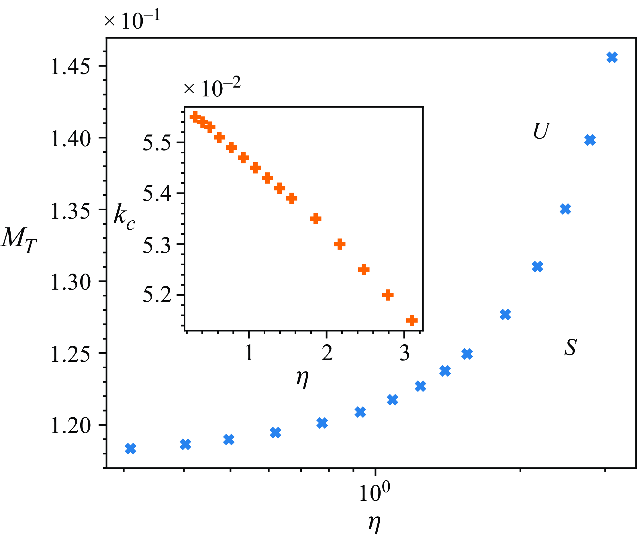
Figure 16. Variation of the critical values of the thermal Marangoni number $M_T$
in the case of a pure monotonic thermocapillary instability with the Soret coefficient
$M_T$
in the case of a pure monotonic thermocapillary instability with the Soret coefficient $\eta$
in the case of heating at the substrate
$\eta$
in the case of heating at the substrate $\mathcal{Q}=1$
at
$\mathcal{Q}=1$
at $B=0.01,$ $\Phi =0.01,$ $L=10^{-3},$ $a=7.47,$ $M_S = 0,$ $\Sigma _0=10,$ $G=0.01$
; inset shows variation of the critical wavenumber
$G=0.01$
; inset shows variation of the critical wavenumber $k_c$
with
$k_c$
with $\eta$
. The symbols
$\eta$
. The symbols $U$
and
$U$
and $S$
denote the unstable and stable domains of the system, respectively.
$S$
denote the unstable and stable domains of the system, respectively.
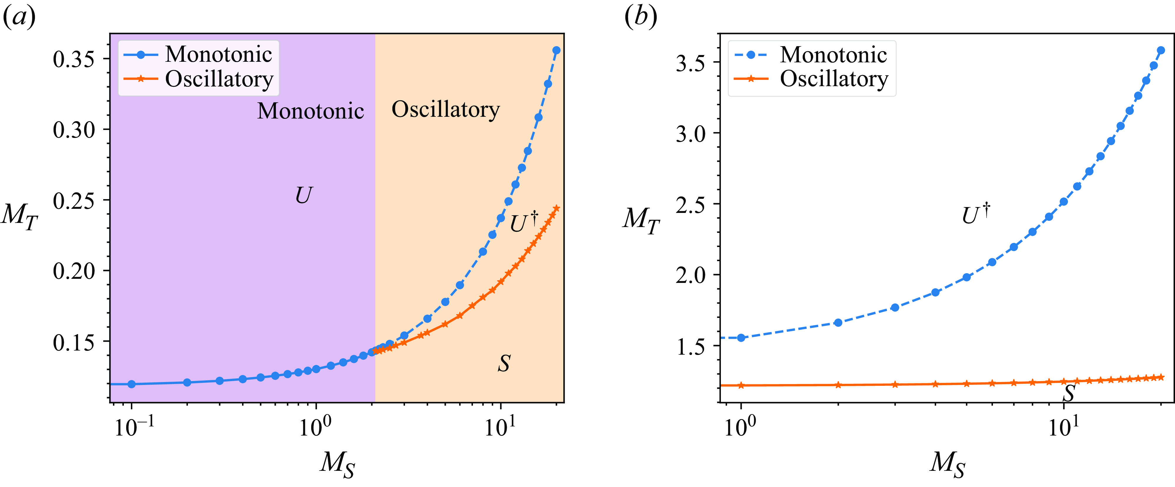
Figure 17. Threshold of the combined soluto-thermocapillary instability shown in the plane $M_T{-} M_S$
in the case of heating at the substrate
$M_T{-} M_S$
in the case of heating at the substrate $\mathcal{Q}=1$
with
$\mathcal{Q}=1$
with $\Phi =0.01,\,\eta =0.31,\,L=10^{-3},\,\Sigma _0=10,\,B=0.01$
. Panels (a) and (b) correspond to
$\Phi =0.01,\,\eta =0.31,\,L=10^{-3},\,\Sigma _0=10,\,B=0.01$
. Panels (a) and (b) correspond to $G=0.01$
and
$G=0.01$
and $G=1$
, respectively. The symbols
$G=1$
, respectively. The symbols $U,\,U^\dagger $
and
$U,\,U^\dagger $
and $S$
represent the domains of one real positive eigenvalue, of two complex conjugate leading eigenvalues with a positive real part, and that of stability, respectively.
$S$
represent the domains of one real positive eigenvalue, of two complex conjugate leading eigenvalues with a positive real part, and that of stability, respectively.
We now consider the onset of the combined soluto-thermocapillary instability. We find that the threshold value of the thermal Marangoni number $M_T$
increases with an increase in the value of the solutal Marangoni number
$M_T$
increases with an increase in the value of the solutal Marangoni number $M_S$
, which implies that solutocapillarity has a stabilising effect, as shown in figure 17. As a reference, in the pure thermocapillary case (
$M_S$
, which implies that solutocapillarity has a stabilising effect, as shown in figure 17. As a reference, in the pure thermocapillary case ( $M_S=0$
), the instability in the case of the given parameter set with
$M_S=0$
), the instability in the case of the given parameter set with $G=0.01$
is monotonic, as seen in figure 11. With an increase of the solutal Marangoni number, the instability turns from monotonic to oscillatory. With a very small value of the modified Galileo number
$G=0.01$
is monotonic, as seen in figure 11. With an increase of the solutal Marangoni number, the instability turns from monotonic to oscillatory. With a very small value of the modified Galileo number $G$
, e.g.,
$G$
, e.g., $G=0.01$
, and with a sufficiently small solutal Marangoni number
$G=0.01$
, and with a sufficiently small solutal Marangoni number $M_S$
,
$M_S$
, $M_S \lesssim 2$
, the emerging instability is monotonic suggesting that thermocapillarity dominates. However, the system undergoes transition from monotonic instability to oscillatory instability with an increase in the value of
$M_S \lesssim 2$
, the emerging instability is monotonic suggesting that thermocapillarity dominates. However, the system undergoes transition from monotonic instability to oscillatory instability with an increase in the value of $M_S$
at approximately
$M_S$
at approximately $M_S = 2$
, as shown in figure 17(a). The oscillatory instability is apparently induced by the disparity between the characteristic times of the thermal diffusivity and the nanoparticle diffusivity, i.e.
$M_S = 2$
, as shown in figure 17(a). The oscillatory instability is apparently induced by the disparity between the characteristic times of the thermal diffusivity and the nanoparticle diffusivity, i.e. $L \ll 1$
. For higher values of
$L \ll 1$
. For higher values of $G$
, e.g.,
$G$
, e.g., $G=1$
, the instability is oscillatory,
$G=1$
, the instability is oscillatory, $M_S=0$
in the pure thermocapillary case, as shown in figure 11. In the combined soluto-thermocapillary case considered here, the instability is oscillatory, as the monotonic boundary remains above the oscillatory one for all
$M_S=0$
in the pure thermocapillary case, as shown in figure 11. In the combined soluto-thermocapillary case considered here, the instability is oscillatory, as the monotonic boundary remains above the oscillatory one for all $M_S\gt 0$
, as presented in figure 17(b). The critical wavenumber
$M_S\gt 0$
, as presented in figure 17(b). The critical wavenumber $k_c$
is presented in figure 18(a), which shows that
$k_c$
is presented in figure 18(a), which shows that $k_c$
weakly depends on
$k_c$
weakly depends on $M_S$
in the case of the monotonic instability, whereas it significantly increases with
$M_S$
in the case of the monotonic instability, whereas it significantly increases with $M_S$
for the oscillatory instability. It is also interesting to note that the value of
$M_S$
for the oscillatory instability. It is also interesting to note that the value of $k_c$
exhibits a discontinuity at
$k_c$
exhibits a discontinuity at $M_S$
corresponding to the change in the instability type. This suggests that the transition from the monotonic to oscillatory instability takes place through the codimension-two point. The critical frequency
$M_S$
corresponding to the change in the instability type. This suggests that the transition from the monotonic to oscillatory instability takes place through the codimension-two point. The critical frequency $\lambda _i$
is presented in figure 18(b). It is found to increase monotonically and almost linearly with
$\lambda _i$
is presented in figure 18(b). It is found to increase monotonically and almost linearly with $M_S$
and collaterally with
$M_S$
and collaterally with $M_T$
along the critical curve.
$M_T$
along the critical curve.
Figure 19 presents the neutral curves $M_T(k)$
for three values of
$M_T(k)$
for three values of $M_S$
with both monotonic and oscillatory branches shown. In the case of
$M_S$
with both monotonic and oscillatory branches shown. In the case of $M_S=0$
displayed in figure 19(a), the oscillatory branch bifurcates off the monotonic one at
$M_S=0$
displayed in figure 19(a), the oscillatory branch bifurcates off the monotonic one at $M_T$
higher than the minimum of the neutral curve, and being a monotonically increasing function of
$M_T$
higher than the minimum of the neutral curve, and being a monotonically increasing function of $k$
, it remains above the critical value of
$k$
, it remains above the critical value of $M_T$
corresponding to the onset of the monotonic instability of the system, as also shown in figure 17. The case of
$M_T$
corresponding to the onset of the monotonic instability of the system, as also shown in figure 17. The case of $M_S=2.1$
presented in figure 19(b), illustrates the emergence of a codimension-two point, so the minimal values of the monotonic and oscillatory branches are attained at the same
$M_S=2.1$
presented in figure 19(b), illustrates the emergence of a codimension-two point, so the minimal values of the monotonic and oscillatory branches are attained at the same $M_T$
, see the borderline between the two domains in figure 17(a). The critical wavenumber
$M_T$
, see the borderline between the two domains in figure 17(a). The critical wavenumber $k_c$
of the oscillatory instability is larger than that of the monotonic instability. This case is in particular interesting due to the dual mechanism of the selection of the type of the emerging instability. Near the threshold of the thermocapillary instability, the emerging instability may be monotonic or oscillatory or of both types, and thus exhibits a competition between the monotonic and oscillatory modes (Brand, Hohenberg & Steinberg Reference Brand, Hohenberg and Steinberg1984). With an increase in
$k_c$
of the oscillatory instability is larger than that of the monotonic instability. This case is in particular interesting due to the dual mechanism of the selection of the type of the emerging instability. Near the threshold of the thermocapillary instability, the emerging instability may be monotonic or oscillatory or of both types, and thus exhibits a competition between the monotonic and oscillatory modes (Brand, Hohenberg & Steinberg Reference Brand, Hohenberg and Steinberg1984). With an increase in $M_S$
, the oscillatory branch bifurcates off the monotonic branch near the minimum of the monotonic branch and descends below it; hence, the emerging instability is oscillatory. The critical wavenumber
$M_S$
, the oscillatory branch bifurcates off the monotonic branch near the minimum of the monotonic branch and descends below it; hence, the emerging instability is oscillatory. The critical wavenumber $k_c$
of the oscillatory instability is larger than that for
$k_c$
of the oscillatory instability is larger than that for $M_S=2.1$
, which is consistent with an increase of
$M_S=2.1$
, which is consistent with an increase of $k_c$
with
$k_c$
with $M_S$
shown in figure 18(a) for the oscillatory instability.
$M_S$
shown in figure 18(a) for the oscillatory instability.
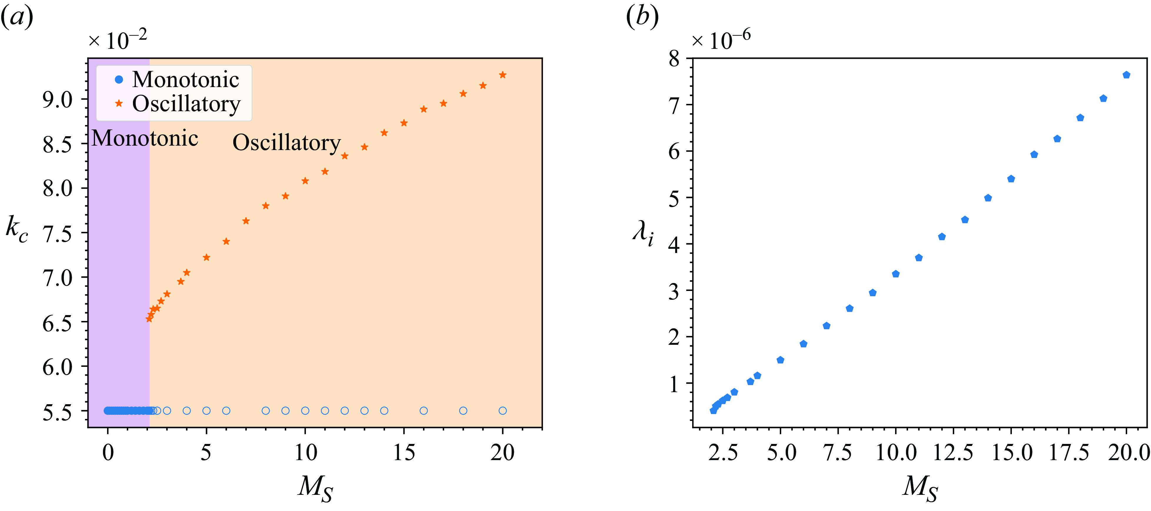
Figure 18. The case of heating at the substrate $\mathcal{Q}=1$
at
$\mathcal{Q}=1$
at $\Phi =0.01,$ $\eta =0.31,$ $L=10^{-3},$ $a=7.47,$ $\Sigma _0=10,$ $G=0.01,$ $B=0.01$
. (a) Variation of the critical wavenumber
$B=0.01$
. (a) Variation of the critical wavenumber $k_c$
with the solutal Marangoni number
$k_c$
with the solutal Marangoni number $M_S$
along the critical curve shown in figure 17(a). Note that the values of
$M_S$
along the critical curve shown in figure 17(a). Note that the values of $k$
along the monotonic curve protruding into the domain of the oscillatory instability which are shown by the hollow circles are not critical. (b) Variation of the critical frequency
$k$
along the monotonic curve protruding into the domain of the oscillatory instability which are shown by the hollow circles are not critical. (b) Variation of the critical frequency $\lambda _i$
with the solutal Marangoni number
$\lambda _i$
with the solutal Marangoni number $M_S$
along the critical curve presented in figure 17(a) in the domain of the oscillatory instability.
$M_S$
along the critical curve presented in figure 17(a) in the domain of the oscillatory instability.

Figure 19. Neutral curves $M_T(k)$
in the case of heating at the substrate
$M_T(k)$
in the case of heating at the substrate $\mathcal{Q}=1$
with
$\mathcal{Q}=1$
with $\Phi =0.01,$ $\eta =0.31,$ $L=10^{-3},$ $a=7.47,$ $\Sigma _0=10,$ $G=0.01$
and
$G=0.01$
and $B=0.01$
. Panels (a), (b) and (c) display the structure of the neutral curves for the monotonic
$B=0.01$
. Panels (a), (b) and (c) display the structure of the neutral curves for the monotonic $(\circ )$
and oscillatory branches
$(\circ )$
and oscillatory branches $(\star )$
for
$(\star )$
for $M_S=0,\,2.1$
and
$M_S=0,\,2.1$
and $20$
, respectively. Panel (b) shows the emergence of the co-dimension two point at
$20$
, respectively. Panel (b) shows the emergence of the co-dimension two point at $M_S=2.1$
. The symbols
$M_S=2.1$
. The symbols $U,\,U^\dagger $
and
$U,\,U^\dagger $
and $S$
represent the domains of one real positive eigenvalue, two leading complex conjugate eigenvalues with a positive real part, and that of the system stability, respectively.
$S$
represent the domains of one real positive eigenvalue, two leading complex conjugate eigenvalues with a positive real part, and that of the system stability, respectively.
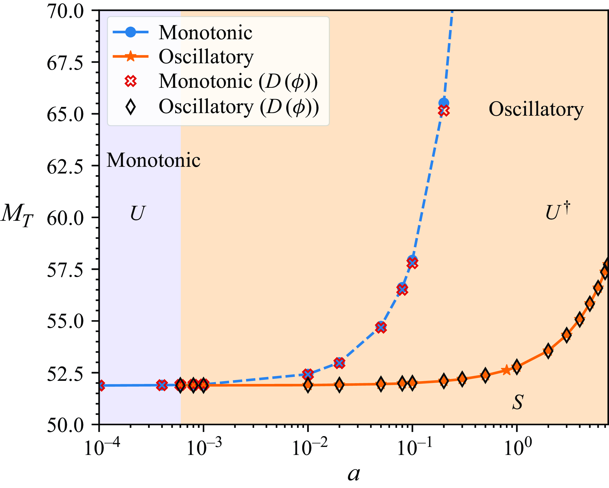
Figure 20. Variation of the critical thermal Marangoni number $M_T$
with the thermal conductivity stratification parameter
$M_T$
with the thermal conductivity stratification parameter $a$
in the case of heating at the substrate
$a$
in the case of heating at the substrate $\mathcal{Q}=1$
with
$\mathcal{Q}=1$
with $\Phi =0.01,$ $\eta =0.31,$ $L=10^{-3},$ $M_S = 0,$ $\zeta =0,$ $G=0$
and
$G=0$
and $B=0.01$
. The symbols
$B=0.01$
. The symbols $U,\,U^\dagger $
and
$U,\,U^\dagger $
and $S$
denote the domains with one real positive eigenvalue, with two leading complex conjugate eigenvalues with a positive real part, and that of stability, respectively. The
$S$
denote the domains with one real positive eigenvalue, with two leading complex conjugate eigenvalues with a positive real part, and that of stability, respectively. The $\circ$
and
$\circ$
and $\star$
symbols denote, respectively, the onset of the monotonic and oscillatory instabilities in the case of a constant Brownian diffusivity
$\star$
symbols denote, respectively, the onset of the monotonic and oscillatory instabilities in the case of a constant Brownian diffusivity $D_B$
, whereas
$D_B$
, whereas $\times$
and
$\times$
and $\diamond$
symbols represent, respectively, the onset of monotonic and oscillatory instability with nanoparticle concentration-dependent Brownian diffusion
$\diamond$
symbols represent, respectively, the onset of monotonic and oscillatory instability with nanoparticle concentration-dependent Brownian diffusion $D(\phi )$
given by (2.5b
).
$D(\phi )$
given by (2.5b
).
4.4. Influence of the thermal conductivity stratification of the nanofluid
In this subsection, we study the effect of thermal conductivity stratification of the nanofluid on the type of Marangoni instability. To simplify the analysis, we assume here the absence of gravity, $G=0$
, the non-deformability of the interface,
$G=0$
, the non-deformability of the interface, $\zeta =0$
, and the absence of solutocapillarity,
$\zeta =0$
, and the absence of solutocapillarity, $M_S=0$
. Figure 20 displays the variation of the critical thermal Marangoni number
$M_S=0$
. Figure 20 displays the variation of the critical thermal Marangoni number $M_T$
with the thermal conductivity stratification parameter
$M_T$
with the thermal conductivity stratification parameter $a$
. We find that the monotonic instability sets in for sufficiently small values of
$a$
. We find that the monotonic instability sets in for sufficiently small values of $a\lt a_c\sim 6\times 10^{-4}$
. However, the oscillatory instability emerges when the thermal conductivity stratification further increases. Therefore, fluids with nanoparticles with a low thermal conductivity undergo the monotonic instability, whereas those made of metals, i.e. with a higher thermal conductivity, for instance, alumina, copper, etc. (Buongiorno Reference Buongiorno2006; Coccia, Tomassetti & Di Nicola et al. Reference Coccia, Tomassetti and Di Nicola2021), are expected to exhibit oscillatory instability.
$a\lt a_c\sim 6\times 10^{-4}$
. However, the oscillatory instability emerges when the thermal conductivity stratification further increases. Therefore, fluids with nanoparticles with a low thermal conductivity undergo the monotonic instability, whereas those made of metals, i.e. with a higher thermal conductivity, for instance, alumina, copper, etc. (Buongiorno Reference Buongiorno2006; Coccia, Tomassetti & Di Nicola et al. Reference Coccia, Tomassetti and Di Nicola2021), are expected to exhibit oscillatory instability.
We recall that throughout this paper, we used a constant value for the Brownian diffusion coefficient. As follows from (2.19), with low values of the thermal conductivity parameter $a$
, the coefficient of the term linear in
$a$
, the coefficient of the term linear in $\phi$
for
$\phi$
for $D(\phi )$
in equation (2.19) is larger than
$D(\phi )$
in equation (2.19) is larger than $a$
; therefore, it may be inferred that the variation of the Brownian diffusivity with particle concentration must be accounted for. Figure 20 also demonstrates the threshold of the thermocapillary instability for the case in which the nanoparticle concentration-dependent Brownian diffusion coefficient
$a$
; therefore, it may be inferred that the variation of the Brownian diffusivity with particle concentration must be accounted for. Figure 20 also demonstrates the threshold of the thermocapillary instability for the case in which the nanoparticle concentration-dependent Brownian diffusion coefficient $D(\phi )$
given by (2.19) is taken into account. We find that the critical value of
$D(\phi )$
given by (2.19) is taken into account. We find that the critical value of $M_T$
based on the use of the concentration-dependent Brownian diffusion coefficient given by Batchelor (Reference Batchelor1976) differs from
$M_T$
based on the use of the concentration-dependent Brownian diffusion coefficient given by Batchelor (Reference Batchelor1976) differs from $M_T$
determined using a constant Brownian diffusion coefficient
$M_T$
determined using a constant Brownian diffusion coefficient $D_B$
by less than
$D_B$
by less than $2\,\%$
. We also find that the instability type, either monotonic or oscillatory, and the transition value of
$2\,\%$
. We also find that the instability type, either monotonic or oscillatory, and the transition value of $a=a_c$
from one to another are not affected by whether a constant or particle concentration-dependent Brownian diffusion coefficient is used. Moreover, we note that the variation of the threshold of the oscillatory thermocapillary instability up to the upper bound of the Hashin–Shtrikman interval (Hashin & Shtrikman Reference Hashin and Shtrikman1962; Keblinski et al. Reference Keblinski, Prasher and Eapen2008) remains smooth, and an increase in
$a=a_c$
from one to another are not affected by whether a constant or particle concentration-dependent Brownian diffusion coefficient is used. Moreover, we note that the variation of the threshold of the oscillatory thermocapillary instability up to the upper bound of the Hashin–Shtrikman interval (Hashin & Shtrikman Reference Hashin and Shtrikman1962; Keblinski et al. Reference Keblinski, Prasher and Eapen2008) remains smooth, and an increase in $a$
leads to a substantial increase in
$a$
leads to a substantial increase in $M_T$
(not shown).
$M_T$
(not shown).
Figure 21(a) demonstrates that the critical wavenumber $k_c$
for the onset of Marangoni instability lies in the short-wave domain for both monotonic and oscillatory instabilities. The critical wavenumber slowly increases with
$k_c$
for the onset of Marangoni instability lies in the short-wave domain for both monotonic and oscillatory instabilities. The critical wavenumber slowly increases with $a$
continuously changing through the transition value of
$a$
continuously changing through the transition value of $a=a_c$
from the monotonic to oscillatory domains. Figure 21(b) shows an increase in the critical frequency
$a=a_c$
from the monotonic to oscillatory domains. Figure 21(b) shows an increase in the critical frequency $\lambda _i$
with an increase in
$\lambda _i$
with an increase in $a$
. Again, the difference between the results based on a constant
$a$
. Again, the difference between the results based on a constant $D_B$
and nanoparticle concentration-dependent forms for the Brownian diffusivity
$D_B$
and nanoparticle concentration-dependent forms for the Brownian diffusivity $D(\phi )$
is minor.
$D(\phi )$
is minor.
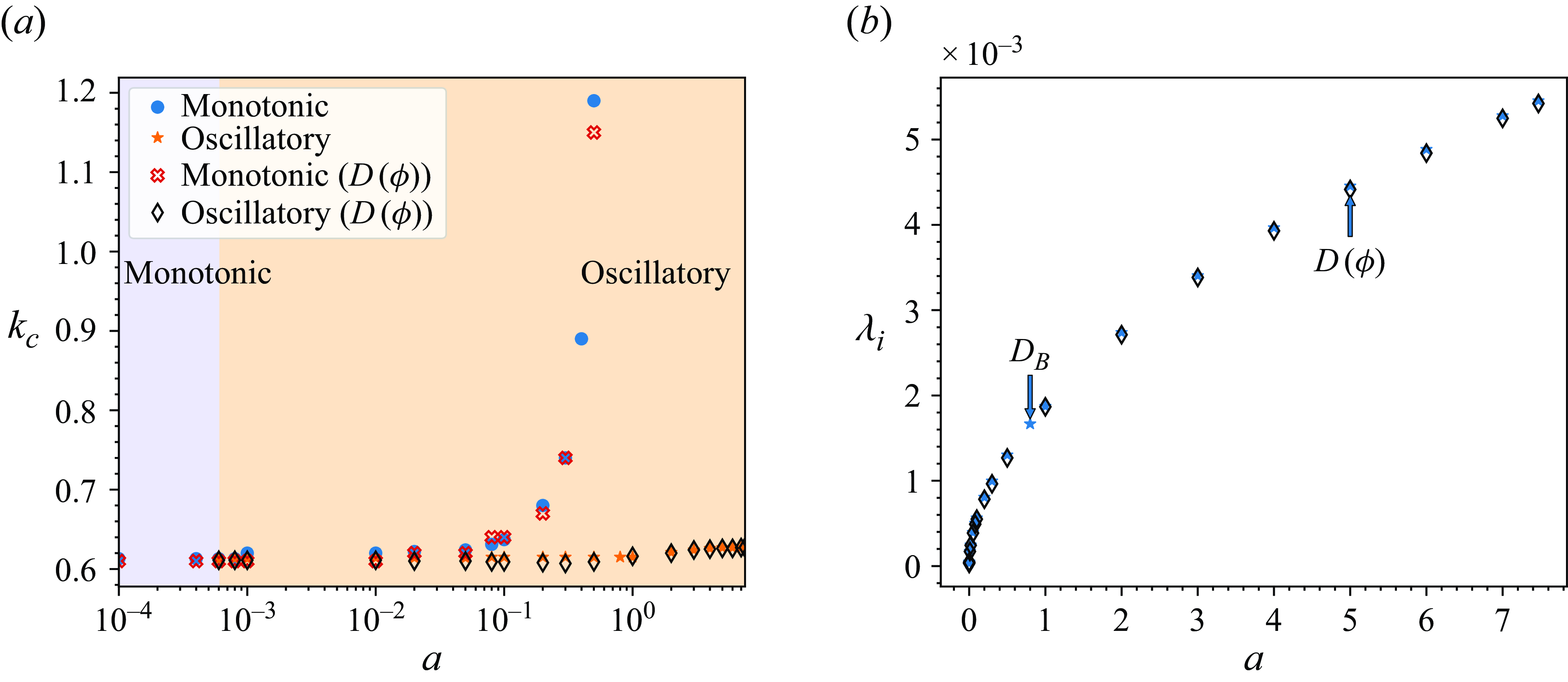
Figure 21. The case of heating at the substrate $\mathcal{Q}=1$
at
$\mathcal{Q}=1$
at $\Phi =0.01,$ $\eta =0.31,$ $L=10^{-3},$ $M_S = 0,$ $\zeta =0,$ $G=0$
and
$G=0$
and $B=0.01$
. (a) Variation of the critical wavenumber
$B=0.01$
. (a) Variation of the critical wavenumber $k_c$
with the thermal conductivity stratification parameter
$k_c$
with the thermal conductivity stratification parameter $a$
. The
$a$
. The $\circ$
and
$\circ$
and $\star$
symbols show
$\star$
symbols show $k_c$
of the monotonic and oscillatory instabilities, respectively, when a constant Brownian diffusivity
$k_c$
of the monotonic and oscillatory instabilities, respectively, when a constant Brownian diffusivity $D_B$
is used, whereas the
$D_B$
is used, whereas the $\times$
and
$\times$
and $\diamond$
symbols denote
$\diamond$
symbols denote $k_c$
of the monotonic and oscillatory instability, respectively, when the nanoparticle concentration-dependent Brownian diffusion
$k_c$
of the monotonic and oscillatory instability, respectively, when the nanoparticle concentration-dependent Brownian diffusion $D(\phi )$
is used. The circles in the oscillatory domain denote the values of the wavenumber corresponding to the monotonic mode and they do not represent critical values. The
$D(\phi )$
is used. The circles in the oscillatory domain denote the values of the wavenumber corresponding to the monotonic mode and they do not represent critical values. The $U,\,U^\dagger, $
and
$U,\,U^\dagger, $
and $S$
symbols represent the domains of monotonic instability, oscillatory instability and stability of the system, respectively. (b) Variation of the critical frequency
$S$
symbols represent the domains of monotonic instability, oscillatory instability and stability of the system, respectively. (b) Variation of the critical frequency $\lambda _i$
with the thermal conductivity stratification parameter
$\lambda _i$
with the thermal conductivity stratification parameter $a$
in the domain where the oscillatory instability sets in. The
$a$
in the domain where the oscillatory instability sets in. The $\star$
and
$\star$
and $\diamond$
symbols represent the critical frequency
$\diamond$
symbols represent the critical frequency $\lambda _i$
corresponding to a constant and nanoparticle concentration-dependent forms for the Brownian diffusivity,
$\lambda _i$
corresponding to a constant and nanoparticle concentration-dependent forms for the Brownian diffusivity, $D_B$
and
$D_B$
and $D(\phi )$
, respectively.
$D(\phi )$
, respectively.
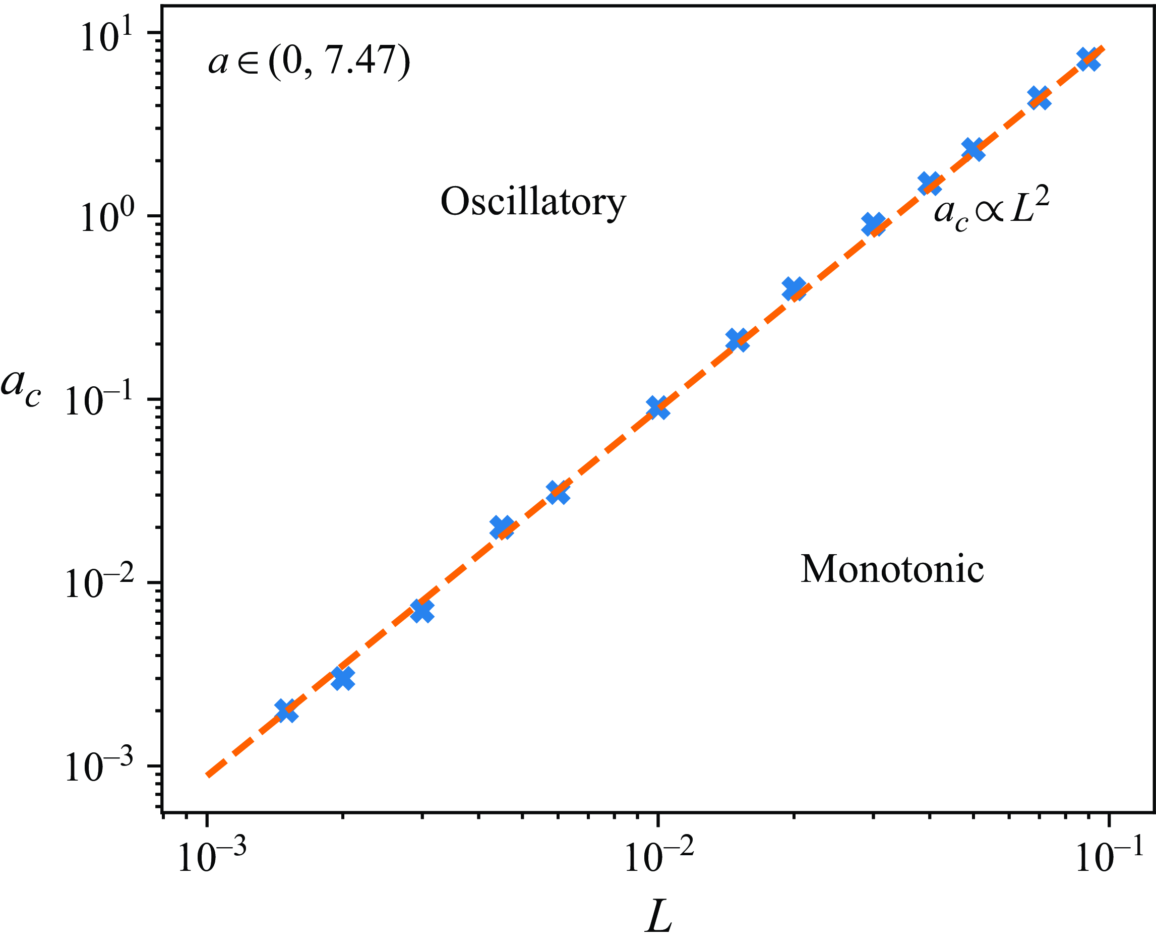
Figure 22. Variation of the critical thermal conductivity stratification parameter $a_c$
with the Lewis number
$a_c$
with the Lewis number $L$
in the case of heating at the substrate
$L$
in the case of heating at the substrate $\mathcal{Q}=1$
with
$\mathcal{Q}=1$
with $\Phi =0.01,$ $\eta =0.31,$ $M_S = 0,$ $\zeta =0,$ $G=0$
and
$G=0$
and $B=0.01$
. The thermal conductivity stratification parameter
$B=0.01$
. The thermal conductivity stratification parameter $a$
varies in the domain
$a$
varies in the domain $a\in (0,7.47)$
. The dashed line represents the data fit
$a\in (0,7.47)$
. The dashed line represents the data fit $a_c\propto L^2$
with the factor of
$a_c\propto L^2$
with the factor of $8.80\times 10^2$
.
$8.80\times 10^2$
.
The variation of the critical thermal stratification parameter $a_c$
for the onset of oscillatory instability with the Lewis number
$a_c$
for the onset of oscillatory instability with the Lewis number $L$
is shown in figure 22 for the case of a layer with the non-deformable interface. It is found that in the limit of small
$L$
is shown in figure 22 for the case of a layer with the non-deformable interface. It is found that in the limit of small $L$
, the value of
$L$
, the value of $a_c$
is proportional to
$a_c$
is proportional to $L^2$
. We note that having a large value for the proportionality factor, the nanofluid layer with the particle concentration diffusion time scale comparable to the thermal diffusion time scale, e.g., with the Lewis number
$L^2$
. We note that having a large value for the proportionality factor, the nanofluid layer with the particle concentration diffusion time scale comparable to the thermal diffusion time scale, e.g., with the Lewis number $L\sim O(10^{-1})$
, requires a significantly higher value of the thermal stratification parameter
$L\sim O(10^{-1})$
, requires a significantly higher value of the thermal stratification parameter $a=a_c$
for the system to switch from the monotonic to oscillatory instability. However, with a sufficiently low value of the Lewis number
$a=a_c$
for the system to switch from the monotonic to oscillatory instability. However, with a sufficiently low value of the Lewis number $L\ll 1$
, the oscillatory instability occurs already at a very low thermal conductivity stratification parameter
$L\ll 1$
, the oscillatory instability occurs already at a very low thermal conductivity stratification parameter $a_c \ll 1$
. We also note that the critical value
$a_c \ll 1$
. We also note that the critical value $a_c$
in figure 22 will be different for a layer when the interfacial deformation is present. The effect of the interfacial deformation via the dimensionless surface tension number
$a_c$
in figure 22 will be different for a layer when the interfacial deformation is present. The effect of the interfacial deformation via the dimensionless surface tension number $\Sigma _0$
on the variation of
$\Sigma _0$
on the variation of $a_c$
will be discussed elsewhere.
$a_c$
will be discussed elsewhere.
4.5. Eigenfunctions and physical mechanism
We examine the underlying physical mechanism driving the instabilities of our system by presenting sets of eigenfunctions near the criticality, i.e. the critical wavenumber $k_c$
, where the growth rate is the highest and the value of the control parameter, here the solutal or the thermal Marangoni number, reaches the minimal value along the neutral curve.
$k_c$
, where the growth rate is the highest and the value of the control parameter, here the solutal or the thermal Marangoni number, reaches the minimal value along the neutral curve.
The purely solutocapillary mechanism of instability in the case of a nanofluid layer cooled at the substrate works in the following way. The concentration profile in this configuration exhibits a gravity stable stratification, e.g., a higher concentration of heavier nanoparticles near the substrate compared with their lower concentration near the interface. Now, suppose that due to an infinitesimal disturbance, a fluid packet with a higher concentration and lower temperature from underneath the interface is displaced towards it, where the surface tension decreases with the concentration. This creates a cooler spot with a higher concentration at the layer interface. If the thermocapillary effect is absent, $\sigma^\ast_{T^\ast}=0$
, a higher concentration spot represents a spot with a lower surface tension inducing flow along the interface emanating from it towards the domain with a higher surface tension which is that of a lower concentration. The flow is then fed by mass conservation bringing fresh fluid packets with even higher concentration from the bulk.
$\sigma^\ast_{T^\ast}=0$
, a higher concentration spot represents a spot with a lower surface tension inducing flow along the interface emanating from it towards the domain with a higher surface tension which is that of a lower concentration. The flow is then fed by mass conservation bringing fresh fluid packets with even higher concentration from the bulk.
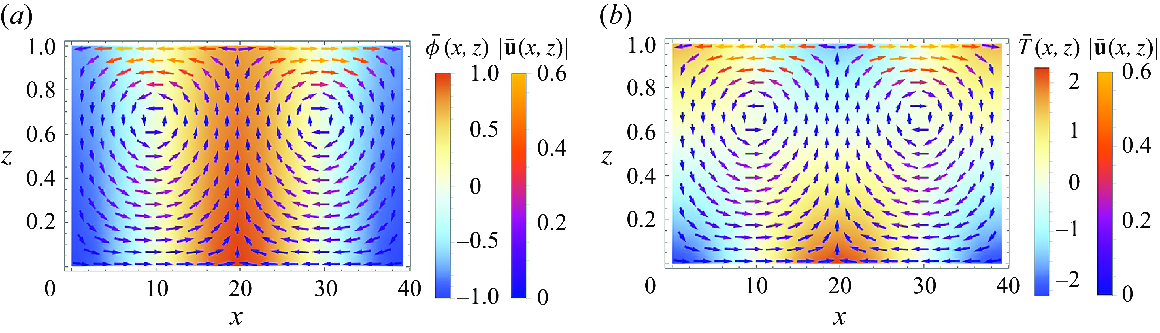
Figure 23. Normalised eigenfunctions of the EVP (3.7) in the case of cooling at the substrate $\mathcal{Q} = -1$
for the critical wavenumber
$\mathcal{Q} = -1$
for the critical wavenumber $k_c = 0.16$
with
$k_c = 0.16$
with $L=10^{-3},$ $\Phi =0.01,$ $\eta =0.31,$ $a=7.47,$ $B=0.01,$ $\Sigma _0\approx 2\times 10^{4},$ $G=6.71,$ $M_S = 23,\,M_T=0$
and
$M_S = 23,\,M_T=0$
and $\lambda =1.1707\times 10^{-7}.$
The eigenfunctions
$\lambda =1.1707\times 10^{-7}.$
The eigenfunctions $\bar {\phi }(x,z)$
and
$\bar {\phi }(x,z)$
and $\bar {T}(x,z)$
superimposed with the velocity vector field
$\bar {T}(x,z)$
superimposed with the velocity vector field $\bar {\textbf{u}}(x,z)$
are shown in panels (a) and (b), respectively. The velocity vector field
$\bar {\textbf{u}}(x,z)$
are shown in panels (a) and (b), respectively. The velocity vector field $\bar {\textbf{u}}(x,z)$
shows the convective flow driven from the low surface tension spot (high nanoparticle concentration) towards that of the high surface tension (low nanoparticle concentration).
$\bar {\textbf{u}}(x,z)$
shows the convective flow driven from the low surface tension spot (high nanoparticle concentration) towards that of the high surface tension (low nanoparticle concentration).
Figure 23 displays a typical set of the eigenfunctions for the monotonic instability emerging in the case of the system cooled at the substrate. Panels (a) and (b) present the eigenfunctions for the concentration disturbances $\bar {\phi } (x,z)$
and those for the temperature
$\bar {\phi } (x,z)$
and those for the temperature $\bar {T}(x,z)$
, respectively, both superimposed with the flow velocity field presented by the velocity vectors. In figure 23(a) of nanoparticle concentration
$\bar {T}(x,z)$
, respectively, both superimposed with the flow velocity field presented by the velocity vectors. In figure 23(a) of nanoparticle concentration $\bar {\phi }(x,z)$
, we observe a rising flow in the high-concentration domain which is driven by the solutocapillary shear stress towards the low-concentration domain forming a descending flow there. Gravity, thermal diffusion and viscosity of the fluid all act against the destabilising solutocapillary effect and saturate the instability, so that the latter is monotonic. It is interesting to note that both fields of concentration and temperature disturbances
$\bar {\phi }(x,z)$
, we observe a rising flow in the high-concentration domain which is driven by the solutocapillary shear stress towards the low-concentration domain forming a descending flow there. Gravity, thermal diffusion and viscosity of the fluid all act against the destabilising solutocapillary effect and saturate the instability, so that the latter is monotonic. It is interesting to note that both fields of concentration and temperature disturbances $\bar {\phi }$
and
$\bar {\phi }$
and $\bar {T}$
, respectively, form stripes. This is explained by the fact that the functions
$\bar {T}$
, respectively, form stripes. This is explained by the fact that the functions $\phi$
and
$\phi$
and $\theta$
found from the numerical solution of the eigenvalue problem (3.7) weakly vary with the height
$\theta$
found from the numerical solution of the eigenvalue problem (3.7) weakly vary with the height $z$
when the former retains its sign, whereas the latter changes its sign.
$z$
when the former retains its sign, whereas the latter changes its sign.

Figure 24. Normalised eigenfunctions of the EVP (3.7) in the case of heating at the substrate $\mathcal{Q} = 1$
for the critical wavenumber
$\mathcal{Q} = 1$
for the critical wavenumber $k_c = 0.18$
with
$k_c = 0.18$
with $L=10^{-3},$ $\Phi =0.01,$ $\eta =0.31,$ $a=7.47,$ $B=0.01,$ $\Sigma _0=10,$ $G=1,$ $M_S =0,\,M_T=1.22\ \text{and}\ \lambda =2.0773\times 10^{-6}+3.6965\times 10^{-5}i.$
The eigenfunctions for the concentration
$M_S =0,\,M_T=1.22\ \text{and}\ \lambda =2.0773\times 10^{-6}+3.6965\times 10^{-5}i.$
The eigenfunctions for the concentration $\bar {\phi }(x,z)$
and temperature
$\bar {\phi }(x,z)$
and temperature $\bar {T}(x,z)$
disturbances superimposed with the velocity vector field
$\bar {T}(x,z)$
disturbances superimposed with the velocity vector field $|\bar {\textbf{u}}(x,z)|$
, are shown in panels (a) and (b), respectively.
$|\bar {\textbf{u}}(x,z)|$
, are shown in panels (a) and (b), respectively.
We next present a set of eigenfunctions in the case of a pure oscillatory thermocapillary instability in a layer heated at the substrate in figure 24. Both $\varphi (z)$
and
$\varphi (z)$
and $\theta (z)$
are found to weakly depend on
$\theta (z)$
are found to weakly depend on $z$
, so both eigenfunctions
$z$
, so both eigenfunctions $\bar {\phi }(x,z)$
and
$\bar {\phi }(x,z)$
and $\bar {T}(x,z)$
display rolls contained between the extrema of the interfacial deformation. Since the depression of the interface is closer to a hot substrate and the interfacial elevation is farther away from it, their temperatures correspond to the maximum and the minimum of the interfacial temperature, respectively. This creates thermocapillary shear stresses directed away from the depression where the surface tension is the lowest to the elevation where the surface tension is the highest, thereby driving a flow within the entire bulk by means of fluid viscosity. In figure 24(b) of
$\bar {T}(x,z)$
display rolls contained between the extrema of the interfacial deformation. Since the depression of the interface is closer to a hot substrate and the interfacial elevation is farther away from it, their temperatures correspond to the maximum and the minimum of the interfacial temperature, respectively. This creates thermocapillary shear stresses directed away from the depression where the surface tension is the lowest to the elevation where the surface tension is the highest, thereby driving a flow within the entire bulk by means of fluid viscosity. In figure 24(b) of $\bar {T}(x,z)$
, we note the formation of the upwelling flow in the higher-temperature domain and the descending flow in the lower-temperature domain. As in the case shown in figure 23, the patterns shown in the profiles of the concentration and temperature disturbances eigenfunctions are stripes, since their amplitude functions
$\bar {T}(x,z)$
, we note the formation of the upwelling flow in the higher-temperature domain and the descending flow in the lower-temperature domain. As in the case shown in figure 23, the patterns shown in the profiles of the concentration and temperature disturbances eigenfunctions are stripes, since their amplitude functions $\phi$
and
$\phi$
and $\theta$
, respectively, depend weakly on
$\theta$
, respectively, depend weakly on $z$
. However, there is a phase shift between these stripes. This phase shift is due to the fact that in one of them, the real part dominates its imaginary part, whereas the opposite takes place in the other.
$z$
. However, there is a phase shift between these stripes. This phase shift is due to the fact that in one of them, the real part dominates its imaginary part, whereas the opposite takes place in the other.
4.6. Incompressibility simplification
The fluid density, as described in § 2.1, varies with space, time and depends on the particle concentration which itself evolves in time and space. Therefore, generally speaking, the fluid in the problem at hand is ‘compressible’. It is possible to rewrite the non-dimensional form of the nanofluid continuity equation (2.13a ) as
 \begin{equation} \nabla \cdot \textbf{u} = -\left (\rho _{np}-1\right )\phi _m\left [P\phi _t + \nabla \cdot \left (\phi \textbf{u}\right )\right ]. \end{equation}
Based on (4.1) and on the nanoparticle mass flux balance equation (2.13d ), the divergence of the velocity vector is obtained in the form
 \begin{equation} \nabla \cdot \textbf{u} = -L\left (\rho _{np}-1\right ) \phi _m\left [\nabla ^2\phi + \nabla \cdot \left (\eta \phi \nabla T\right )\right ]. \end{equation}
The right-hand side of (4.2) represents the deviation of the full ‘compressible’ system from an incompressible one. Assuming that for a moderately dense nanofluid in the case of a small Lewis number $L$
satisfying the condition
$L$
satisfying the condition $L\in (10^{-4},10^{-2} )$
, the parameter
$L\in (10^{-4},10^{-2} )$
, the parameter $L(\rho _{np}-1)$
is
$L(\rho _{np}-1)$
is $O (10^{-4}-10^{-2} )$
. Thus, (4.2) suggests that the nanofluid system at hand can be, by neglecting its right-hand side, simplified by imposing its ‘incompressibility’. The question is now about the implications of this simplification.
$O (10^{-4}-10^{-2} )$
. Thus, (4.2) suggests that the nanofluid system at hand can be, by neglecting its right-hand side, simplified by imposing its ‘incompressibility’. The question is now about the implications of this simplification.
We now compare the results obtained for the problem governed in its full formulation by the EVP (3.7) with a non-uniform density depending on the space-time dependent particle concentration, and in this case, the problem is referred to as ‘compressible’, with those obtained for a simplified problem where the right-hand side of (4.2) is neglected and the rest of the governing equations and boundary conditions remain with no change. This simplified formulation will be referred to as an ‘incompressible’ one. In some sense, the latter is akin to the Boussinesq approximation where the density is assumed to be constant except for allowing for the buoyancy force arising from the variation in the fluid density.
Figure 25(a) illustrates the comparison between the neutral curve $M_S(k)$
for a pure solutocapillary instability in the case of cooling at the substrate for compressible and incompressible formulations of the problem. We observe that the neutral curve of the simplified incompressible problem displays a close match with the neutral curve obtained for the compressible formulation. Note the difference between the two which does not exceed 2 %. Further, figure 25(b) illustrates an excellent agreement between the variation of the critical thermal Marangoni number
$M_S(k)$
for a pure solutocapillary instability in the case of cooling at the substrate for compressible and incompressible formulations of the problem. We observe that the neutral curve of the simplified incompressible problem displays a close match with the neutral curve obtained for the compressible formulation. Note the difference between the two which does not exceed 2 %. Further, figure 25(b) illustrates an excellent agreement between the variation of the critical thermal Marangoni number $M_T$
with the thermal conductivity stratification parameter
$M_T$
with the thermal conductivity stratification parameter $a$
for both monotonic and oscillatory instabilities in the case of heating at the substrate. Note that the curves for both the compressible and incompressible formulations almost fully overlap with the maximal difference of
$a$
for both monotonic and oscillatory instabilities in the case of heating at the substrate. Note that the curves for both the compressible and incompressible formulations almost fully overlap with the maximal difference of $1.66\,\%$
. Therefore, we infer that the incompressible simplification can be safely used for a nanofluid with stratification of thermophysical properties. We emphasise that all of the results presented here were obtained without using the incompressibility simplification, but note that this simplification may significantly reduce the numerical effort needed for treatment of the problem.
$1.66\,\%$
. Therefore, we infer that the incompressible simplification can be safely used for a nanofluid with stratification of thermophysical properties. We emphasise that all of the results presented here were obtained without using the incompressibility simplification, but note that this simplification may significantly reduce the numerical effort needed for treatment of the problem.
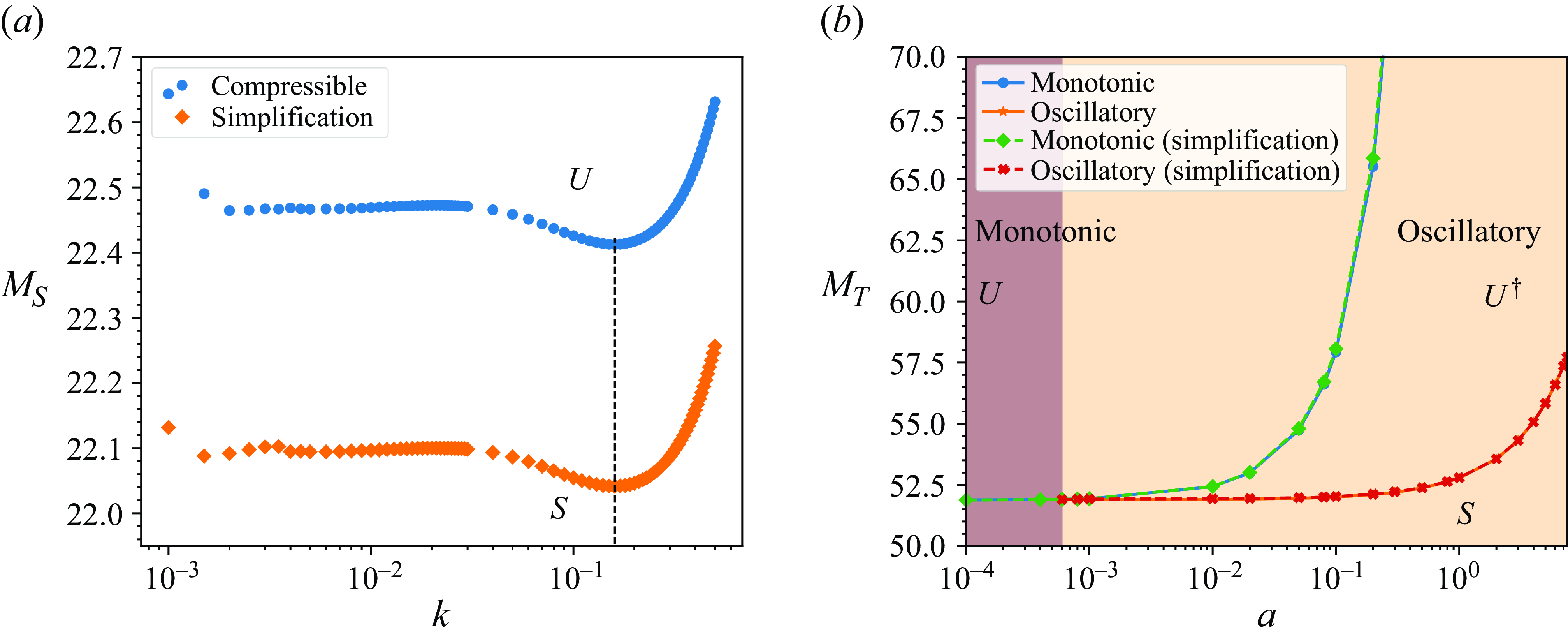
Figure 25. (a) Neutral curves for a pure solutocapillary monotonic instability $M_S(k)$
for the case of cooling at the substrate
$M_S(k)$
for the case of cooling at the substrate $\mathcal{Q}=-1$
with
$\mathcal{Q}=-1$
with $B = 0.01,$ $\Phi =0.01,$ $\eta =0.31,$ $a=7.47,$ $L=10^{-3},$ $M_T = 0,$ $\Sigma _0\approx 2\times 10^{4}$
and
$\Sigma _0\approx 2\times 10^{4}$
and $G=6.71$
. The
$G=6.71$
. The $\circ$
and
$\circ$
and $\diamond$
points correspond to the cases of the full EVP (3.7) and a simplified incompressible formulation, respectively. (b) Variation of the critical thermal Marangoni number with the thermal conductivity stratification parameter
$\diamond$
points correspond to the cases of the full EVP (3.7) and a simplified incompressible formulation, respectively. (b) Variation of the critical thermal Marangoni number with the thermal conductivity stratification parameter $a$
for a pure thermocapillary instability in the case of heating at the substrate
$a$
for a pure thermocapillary instability in the case of heating at the substrate $\mathcal{Q}=1$
with
$\mathcal{Q}=1$
with $\Phi =0.01,$ $\eta =0.31,$ $L=10^{-3},$ $M_S = 0,$ $\zeta =0,$ $G=0,$
and
$G=0,$
and $B=0.01$
. The
$B=0.01$
. The $\circ$
,
$\circ$
, $\star$
,
$\star$
, $\diamond$
and
$\diamond$
and $\times$
points represent the values obtained for the monotonic and oscillatory instabilities based on the full EVP (3.7), respectively, and the monotonic and oscillatory instabilities obtained for a simplified incompressible formulation, respectively. The
$\times$
points represent the values obtained for the monotonic and oscillatory instabilities based on the full EVP (3.7), respectively, and the monotonic and oscillatory instabilities obtained for a simplified incompressible formulation, respectively. The $U,\,U^\dagger, $
and
$U,\,U^\dagger, $
and $S$
symbols represent the domains of monotonic instability, oscillatory instability, and stability of the system, respectively.
$S$
symbols represent the domains of monotonic instability, oscillatory instability, and stability of the system, respectively.
5. Summary and conclusions
In this paper, we present a set of model governing equations and boundary conditions describing the dynamics of a moderately dense heated nanofluid layer with a deformable gas–liquid interface when the carrier fluid is Newtonian. This set of equations is based on continuity, momentum conservation, energy conservation and particle mass conservation equations, and represents an extension of the governing equations valid for dilute binary mixtures. Since, in the case at hand, the mixture is moderately dense, it is unrealistic to assume that its thermophysical properties, e.g., density, dynamic viscosity, thermal conductivity and heat capacity, are constant. Therefore, here they are assumed to depend on the local particle concentration (Maron & Pierce Reference Maron and Pierce1956; Krieger & Dougherty Reference Krieger and Dougherty1959; de Kruif et al. Reference de Kruif, van Iersel, Vrij and Russel1985; Buongiorno Reference Buongiorno2006). We also assume that the Soret effect is present and the thermodiffusion coefficient is also local-particle-concentration dependent (Scriven & Sternling Reference Scriven and Sternling1964; Platten & Legros Reference Platten and Legros1984).
We apply our equations to investigate the stability of a nanofluid layer open to the atmosphere at its deformable interface and subjected to a specified heat flux whether heating or cooling at its underneath support in the gravity field. We also assume that surface tension is both temperature- and particle-concentration dependent, so the thermocapillary and solutocapillary effects are present and accounted for. However, we assume that the considered layer is sufficiently thin, so buoyancy effects arising from an unstable temperature distribution with height is neglected. It is important to emphasise that since the fluid density in our model depends on the local particle concentration varying in both time and space, the system considered here is compressible, so the fluid velocity field is not solenoidal.
We find a steady base state of the system which is written out analytically in terms of the Lambert W function. In the case of cooling at the substrate, the base state exhibits stable stratification in terms of both temperature and particle concentration, which affects directly the fluid density. In contrast, in the case of heating at the substrate, the temperature decreases with height, whereas the particle concentration increases with height; therefore, both conceive several instability mechanisms.
We carry out the linear stability analysis of the base state of the system based on normal mode disturbances. We find that in the case of the system cooled at the substrate, the solutocapillary effect destabilises the system, whereas the thermocapillarity provides a stabilising effect. Interestingly, we note that the neutral curves vary weakly with the disturbance wavenumber and exhibit the emergence of two local minima, one of them located in the long-wave domain, whereas the other is in the finite-wave domain. These two minima compete with each other owing to the variation of the modified Galileo number $G$
and the Soret coefficient
$G$
and the Soret coefficient $\eta$
. We also find that only the finite-wave minimum of the neutral curves is sensitive to variation of the inverse capillary number which is related to the interfacial deformability.
$\eta$
. We also find that only the finite-wave minimum of the neutral curves is sensitive to variation of the inverse capillary number which is related to the interfacial deformability.
In the case of heating at the substrate, the linear stability properties of the system are by far more diverse than in the case of a cooled substrate. We find the emergence of both monotonic and oscillatory instabilities. The former is more typical for low values of the modified Galileo numbers $G$
equivalent to thinner nanofluid layers, mainly driven by thermocapillarity, whereas the latter is typical for moderate values of the Galileo number equivalent to thicker layers and displays a competition between thermocapillarity, solutocapillarity, and gravity. It is interesting to note that the low-Galileo number monotonic instability is long-wave with the critical wavenumber
$G$
equivalent to thinner nanofluid layers, mainly driven by thermocapillarity, whereas the latter is typical for moderate values of the Galileo number equivalent to thicker layers and displays a competition between thermocapillarity, solutocapillarity, and gravity. It is interesting to note that the low-Galileo number monotonic instability is long-wave with the critical wavenumber $k_c$
that follows the well-known scaling with the Biot number
$k_c$
that follows the well-known scaling with the Biot number $B$
for a pure fluid and is one of the two possible scalings found in the literature for a dilute binary mixture, namely
$B$
for a pure fluid and is one of the two possible scalings found in the literature for a dilute binary mixture, namely $k_c \sim B^{1/4}$
. Further, we find that the long-wave thermocapillary instability is stabilised with an increase in the averaged bulk nanoparticle concentration
$k_c \sim B^{1/4}$
. Further, we find that the long-wave thermocapillary instability is stabilised with an increase in the averaged bulk nanoparticle concentration $\Phi$
and in the Soret coefficient
$\Phi$
and in the Soret coefficient $\eta$
. We also reveal that the oscillatory instability for moderate values of
$\eta$
. We also reveal that the oscillatory instability for moderate values of $G$
is finite-wave. For sufficiently high values of
$G$
is finite-wave. For sufficiently high values of $G$
, the instability becomes again monotonic and long-wave driven solely by gravity, referred as to solutal buoyancy instability emerging from an unstable density stratification due to the number of particles which increases with height.
$G$
, the instability becomes again monotonic and long-wave driven solely by gravity, referred as to solutal buoyancy instability emerging from an unstable density stratification due to the number of particles which increases with height.
We have also elucidated the details of the structure of a typical eigenspectrum by following the two leading eigenvalues for different values of the thermal Marangoni number $M_T$
. Among other details, we find that near the emergence of the monotonically growing mode driven by thermocapillarity, there exists another, slowly decreasing with the Marangoni number diffusional mode with a small growth rate which depends on the Lewis number and which is small. Near the inception point where the two modes are comparable, oscillations may emerge.
$M_T$
. Among other details, we find that near the emergence of the monotonically growing mode driven by thermocapillarity, there exists another, slowly decreasing with the Marangoni number diffusional mode with a small growth rate which depends on the Lewis number and which is small. Near the inception point where the two modes are comparable, oscillations may emerge.
When both thermocapillarity and solutocapillarity are active, the instability is monotonic for lower values of the solutal Marangoni numbers, whereas with an increase in the latter, the instability becomes oscillatory via the codimension-two point. Both of these instabilities occur at non-zero wavenumbers with the critical wavenumber for the oscillatory instability higher than that for the monotonic instability.
As mentioned above, since the nanofluid density depends on the local nanoparticle concentration which is time- and space-dependent, the problem is essentially compressible, so the fluid velocity is not solenoidal. This fact poses additional difficulties in the numerical treatment of the linear eigenvalue problem solved to carry out the linear stability analysis. However, despite the fact that all of the results presented in this paper are obtained by solving the full formulation of the problem, we find that in many cases, the difference between the results obtained by solving the problem in its full version and, alternatively, in its simplified version in which the continuity equation is written in the form identical to that of an incompressible fluid is small.
The presence of nanoparticles in a fluid causes a variation in the thermal conductivity of the nanofluid. As mentioned by Buongiorno (Reference Buongiorno2006), thermal conductivity of the nanofluid in the case of alumina particles in water is linear with the local particle concentration with the parameter $a$
referred to here as the thermal conductivity stratification parameter. Our results show that the value of
$a$
referred to here as the thermal conductivity stratification parameter. Our results show that the value of $a$
affects the type of instability, namely, a pure thermocapillary instability is monotonic for small
$a$
affects the type of instability, namely, a pure thermocapillary instability is monotonic for small $a$
and oscillatory when
$a$
and oscillatory when $a$
exceed a certain critical value which is found to be proportional to the square of the Lewis number when the layer interface is non-deformable and in the absence of gravity. This oscillatory instability adds a new mechanism leading to the oscillatory instability induced by the thermal conductivity stratification in addition to other cases known in the literature (Joo Reference Joo1995; Nepomnyashchy & Simanovskii Reference Nepomnyashchy and Simanovskii1995).
$a$
exceed a certain critical value which is found to be proportional to the square of the Lewis number when the layer interface is non-deformable and in the absence of gravity. This oscillatory instability adds a new mechanism leading to the oscillatory instability induced by the thermal conductivity stratification in addition to other cases known in the literature (Joo Reference Joo1995; Nepomnyashchy & Simanovskii Reference Nepomnyashchy and Simanovskii1995).
Most of the instabilities found and discussed here are finite-wave instabilities. However, many of the instabilities, both monotonic and oscillatory dealt with in the similar setting but in the context of dilute binary mixtures (Oron & Nepomnyashchy Reference Oron and Nepomnyashchy2004; Podolny, Oron & Nepomnyashchy Reference Podolny, Oron and Nepomnyashchy2006; Shklyaev et al. Reference Shklyaev, Nepomnyashchy and Oron2007, Reference Shklyaev, Nepomnyashchy and Oron2009) with both constant Soret coefficient and the thermal conductivity of the mixture, were long-wave. To resolve this apparent mismatch, we emphasise that in our setting of a moderately dense mixture with concentration-dependent thermal conductivity and the Soret coefficient, the instabilities become also long-wave in the combined limit of mean particle concentration $\Phi$
, the Soret coefficient
$\Phi$
, the Soret coefficient $\eta$
, the thermal conductivity stratification parameter
$\eta$
, the thermal conductivity stratification parameter $a$
and the Biot number
$a$
and the Biot number $B$
being all very low. In this case, our present theory matches the critical values of the Marangoni number derived by Oron & Nepomnyashchy (Reference Oron and Nepomnyashchy2004) and Podolny et al. (Reference Podolny, Oron and Nepomnyashchy2005) for the layers with either non-deformable or deformable interface. This issue will be further discussed in detail elsewhere.
$B$
being all very low. In this case, our present theory matches the critical values of the Marangoni number derived by Oron & Nepomnyashchy (Reference Oron and Nepomnyashchy2004) and Podolny et al. (Reference Podolny, Oron and Nepomnyashchy2005) for the layers with either non-deformable or deformable interface. This issue will be further discussed in detail elsewhere.
Finally, we emphasise that various analytical approximations have been derived over the years for the thermophysical properties of dilute monodisperse suspensions. At first order with respect to the low local particle concentration, they introduce factors which depend on the respective thermophysical properties of the base fluid and the suspended hard spherical particles. To mention the most prominent ones, these are the expressions for the viscosity (Einstein Reference Einstein1906), thermal conductivity (Maxwell Reference Maxwell1873) and Brownian diffusivity (Batchelor Reference Batchelor1976) of a suspension. In contrast, there are various empirical fits for these properties which are based on experiments conducted with different nanofluids. To bridge between the differences, we have employed the expressions arising from the experimental data, but also compared the results with those based on the theoretical expressions mentioned above. We have found that in terms of the thresholds of the thermosolutal instabilities investigated here, the differences appear to be very small within several percent and without any qualitative discrepancies.
Acknowledgements
We are indebted to the anonymous referees whose valuable comments have contributed to the improvement of the quality of this paper.
Funding
This work is supported by the grant from the European Union’s Horizon 2020 research and innovation program under the Marie Skłodowska–Curie grant agreement number 955612 (NanoPaInt).
Declaration of interests
The authors report no conflict of interest.
Appendix A. Base state of the system
A.1. Nanoparticle concentration-dependent Soret coefficient and thermal conductivity
First, we note that since we seek a quiescent ( ${\textbf u}_0=0$
) equilibrium state of the system, the fluid viscosity does not affect the result. To proceed with this task, we rewrite here for the reader’s convenience the system of equations and boundary conditions given by (2.21), (2.22), and (2.23) with prime denoting differentiation with respect to
${\textbf u}_0=0$
) equilibrium state of the system, the fluid viscosity does not affect the result. To proceed with this task, we rewrite here for the reader’s convenience the system of equations and boundary conditions given by (2.21), (2.22), and (2.23) with prime denoting differentiation with respect to $z$
:
$z$
:
 \begin{align}&\qquad\qquad\qquad p^\prime _{0}= - G -G \phi _m \left (\rho _{np}-1\right ) \phi _0, \end{align}
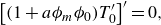 \begin{align}&\qquad\qquad\qquad\quad\,\, \left [(1+a \phi _m \phi _0)T_{0}^\prime \right ]^\prime =0, \end{align}
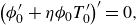 \begin{align}&\qquad\qquad\qquad\qquad \left (\phi ^\prime _{0} + \eta \phi _0 T^\prime _{0}\right )^\prime =0, \end{align}
 \begin{align}&\qquad z=0: \quad \left (1+a\phi _m\phi _0\right )T^\prime _{0} = -\mathcal{Q},\quad \phi ^\prime _{0} + \eta \phi _0 T^\prime _{0} =0, \end{align}
 \begin{align}& z=1: \quad p_0 =0, \quad (1+a \phi _m \phi _0)T^\prime _{0} +B T_0=0, \quad \phi ^\prime _{0} + \eta \phi _0 T^\prime _{0}=0, \end{align}
and
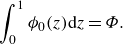 \begin{equation} \int _0^1\phi _0(z){\rm d}z = \Phi . \end{equation}
Integrating once (A1b ) and (A1c ) with the boundary conditions (A2) at the substrate and at the interface, we obtain
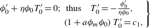 \begin{align} \left . \begin{array}{ll} \phi ^\prime _{0} + \eta \phi _0 T^\prime _{0} =0; & \textrm { thus}\quad T^\prime _{0} = -\frac {\phi ^\prime _{0}}{\eta \phi _0}, \\[5pt] &\left (1+a\phi _m\phi _0\right )T^\prime _{0} = c_1, \end{array}\right \} \end{align}
where $c_1$
is the integration constant. Substituting
$c_1$
is the integration constant. Substituting $T^\prime _{0}$
from the upper equation (A4) into the equation in its lower line, yields
$T^\prime _{0}$
from the upper equation (A4) into the equation in its lower line, yields
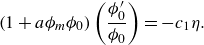 \begin{equation} \left (1+a\phi _m\phi _0\right )\left (\frac {\phi ^\prime _{0}}{\phi _0}\right ) =- c_1\eta . \end{equation}
Equation (A5) is then solved to obtain
 \begin{equation} \phi _0\exp \left (a\phi _m\phi _0\right ) = \exp \left (-c_1\eta z + c_2\right ), \end{equation}
with $c_2$
being another integration constant and which, upon a definition
$c_2$
being another integration constant and which, upon a definition $\chi =a\phi _m\phi _0$
, yields a solution in terms of function
$\chi =a\phi _m\phi _0$
, yields a solution in terms of function $\chi = \chi (z)$
based on the definition of the Lambert W function, (2.25), as
$\chi = \chi (z)$
based on the definition of the Lambert W function, (2.25), as
 \begin{equation} \chi = \mathcal{W}\left (a\phi _m\exp \left (-c_1\eta z+c_2\right )\right ) \end{equation}
and, therefore,
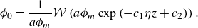 \begin{equation} \phi _0 = \frac {1}{a\phi _m} \mathcal{W}\left (a\phi _m\exp \left (-c_1\eta z + c_2\right )\right ). \end{equation}
Choosing the constant $c_2$
in the form
$c_2$
in the form $c_2 = \ln \gamma + a\phi _m\gamma$
with
$c_2 = \ln \gamma + a\phi _m\gamma$
with $\gamma$
as a new alternative constant of integration to be determined in what follows, and under definition
$\gamma$
as a new alternative constant of integration to be determined in what follows, and under definition
 \begin{equation} \mathcal{P}(z) \equiv \mathcal{W}\left (a\phi _m\gamma \exp \left (-c_1 \eta z + a\phi _m\gamma \right )\right ), \end{equation}
(A8) becomes
 \begin{equation} \phi _0 = \frac {1}{a\phi _m} \mathcal{W}\left (a\phi _m\gamma \exp \left (-c_1 \eta z + a\phi _m\gamma \right )\right ) \equiv \frac {1}{a\phi _m}\mathcal{P}(z). \end{equation}
To proceed, we now need to derive a differentiation rule for $\mathcal{P}$
with respect to
$\mathcal{P}$
with respect to $z$
. By definition of the Lambert function, (2.25),
$z$
. By definition of the Lambert function, (2.25),
 \begin{equation} \mathcal{P} \exp {\left (\mathcal{P}\right )}= a\phi _m\gamma \exp {\left (-c_1 \eta z+a \phi _m \gamma \right )}. \end{equation}
Solving (A11) for $z$
, differentiating
$z$
, differentiating $z$
with respect to
$z$
with respect to $\mathcal{P}$
and employing the inverse function theorem, we find
$\mathcal{P}$
and employing the inverse function theorem, we find
 \begin{equation} {\mathcal{P}^\prime } = -\frac {c_1 \eta \mathcal{P}}{\mathcal{P}+1}. \end{equation}
Using the differentiation rule (A12) and combining (A5) and the heat flux boundary condition (A2a
) at $z=0$
yields
$z=0$
yields $c_1=-\mathcal{Q}$
.
$c_1=-\mathcal{Q}$
.
Equation (A10) now reads
 \begin{equation} \phi _0 = \frac {1}{a\phi _m}\mathcal{W}\left (a\phi _m\gamma \exp \left (\eta \mathcal{Q}z + a\phi _m\gamma \right )\right ) \equiv \frac {1}{a\phi _m}\mathcal{P}(z). \end{equation}
A yet unknown value of $\gamma$
is found from (A3) which represents the conservation of the volume of nanoparticles. For this reason,
$\gamma$
is found from (A3) which represents the conservation of the volume of nanoparticles. For this reason, $\gamma$
from hereon will be denoted as
$\gamma$
from hereon will be denoted as $\gamma (\Phi )$
to stress its origin. The integral
$\gamma (\Phi )$
to stress its origin. The integral $\displaystyle \int _0^1 {\phi _0(z)\,dz}$
can be determined using (A12) with
$\displaystyle \int _0^1 {\phi _0(z)\,dz}$
can be determined using (A12) with $c_1=- \mathcal{Q}$
, and (A3) results in
$c_1=- \mathcal{Q}$
, and (A3) results in
 \begin{align} &\left [1+\mathcal{W}\left (a\phi _m\gamma (\Phi )\exp \left (\eta \mathcal{Q}+a\phi _m\gamma (\Phi )\right ) \right )\right ]^2 -\left [1+\mathcal{W}\left (a\phi _m\gamma (\Phi )\exp \left (a\phi _m\gamma (\Phi )\right )\right )\right ]^2 \notag\\&\quad = 2a\phi _m\eta \mathcal{Q}\Phi . \end{align}
Equation (A14) is solved numerically in terms of $\gamma (\Phi )$
as a function of the parameter set. It is emphasised that the value of
$\gamma (\Phi )$
as a function of the parameter set. It is emphasised that the value of $\gamma (\Phi )$
depends, in addition to
$\gamma (\Phi )$
depends, in addition to $\Phi$
, on four more parameters, namely
$\Phi$
, on four more parameters, namely $a, \phi _m, \eta$
and
$a, \phi _m, \eta$
and $\mathcal{Q}$
.
$\mathcal{Q}$
.
We now proceed to the derivation of the equilibrium temperature $T_0$
based on (A4) with substituting
$T_0$
based on (A4) with substituting $\phi _0$
given by (A13) to obtain
$\phi _0$
given by (A13) to obtain
 \begin{equation} T^\prime _{0} = \frac {-\mathcal{P}^\prime (z)}{\eta \mathcal{P}(z)}. \end{equation}
Hence,
 \begin{equation} T_0 = -\frac {1}{\eta }\left (\ln \mathcal{P}(z)-\ln \mathcal{P}(1)\right ) + c_3, \end{equation}
where $c_3$
is an integration constant to be determined now.
$c_3$
is an integration constant to be determined now.
Using $T_0$
given by (A15b
), we apply the boundary condition (A2b
) and obtain the value of the integration constant
$T_0$
given by (A15b
), we apply the boundary condition (A2b
) and obtain the value of the integration constant $\displaystyle c_3=\frac {\mathcal{Q}}{B}$
. Henceforth, the equilibrium temperature distribution is given by
$\displaystyle c_3=\frac {\mathcal{Q}}{B}$
. Henceforth, the equilibrium temperature distribution is given by
 \begin{align} T_0 ={}&\frac {1}{\eta B}\left [B \ln \left (\frac {1}{a\phi _m}\mathcal{W}\left (\gamma (\Phi ) a\phi _m \exp {\left (\gamma (\Phi ) a\phi _m+\eta \mathcal{Q}\right )}\right )\right )\right .\notag \\&-B\left . \ln \left (\frac {1}{a\phi _m}\mathcal{W}\left (\gamma (\Phi ) a\phi _m \exp {\left (\gamma (\Phi ) a\phi _m+\eta \mathcal{Q} z\right )}\right )\right )+\eta \mathcal{Q}\right ]. \end{align}
Finally, using (A1a
) and the boundary condition $p_0 = 0$
at
$p_0 = 0$
at $z=1$
along with a substitution of
$z=1$
along with a substitution of $\phi _0$
given by (A10), we obtain
$\phi _0$
given by (A10), we obtain
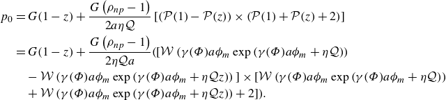 \begin{align} p_0 &= G(1-z) + \frac {G\left (\rho _{np}-1\right )}{2a\eta \mathcal{Q}}\left [\left (\mathcal{P}(1)-\mathcal{P}(z)\right )\times \left (\mathcal{P}(1)+\mathcal{P}(z)+ 2\right )\right ]\nonumber\\&= G (1-z) + \frac {G \left (\rho _{np}-1\right )}{2 \eta \mathcal{Q} a}\Big ( \Big [\mathcal{W}\left (\gamma (\Phi ) a\phi _m \exp {\left (\gamma (\Phi ) a\phi _m+\eta \mathcal{Q}\right )}\right )\nonumber\\&\quad-\mathcal{W}\left (\gamma (\Phi ) a\phi _m \exp {\left (\gamma (\Phi ) a\phi _m+\eta \mathcal{Q} z\right )}\right )\Big ]\times \Big [\mathcal{W}\left (\gamma (\Phi ) a\phi _m \exp {\left (\gamma (\Phi ) a\phi _m+\eta \mathcal{Q}\right )}\right )\nonumber\\&\quad+\mathcal{W}\left (\gamma (\Phi ) a\phi _m \exp {\left (\gamma (\Phi ) a\phi _m+\eta \mathcal{Q} z\right )}\right )+2\Big ]\Big ). \end{align}
In the particular case of $a = 0$
, (A1b
) and (A1c
) are easily solved and the following equilibrium state is obtained:
$a = 0$
, (A1b
) and (A1c
) are easily solved and the following equilibrium state is obtained:
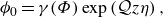 \begin{align}&\qquad\qquad\qquad\qquad\quad \phi _0 = \gamma (\Phi )\exp \left (\mathcal{Q}z\eta \right ), \end{align}
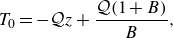 \begin{align}&\qquad\qquad\qquad\qquad\quad T_0 = -\mathcal{Q}z + \frac {\mathcal{Q}(1+B)}{B}, \end{align}
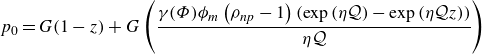 \begin{align}& p_0 = G(1-z) + G \left (\frac {\gamma (\Phi ) \phi _m \left (\rho _{np}-1\right ) \left (\exp \left (\eta \mathcal{Q}\right )-\exp \left (\eta \mathcal{Q}z\right )\right )}{\eta \mathcal{Q}}\right ) \end{align}
with
 \begin{equation} \gamma (\Phi )=\frac {\Phi \mathcal{Q} \eta }{\exp {(\mathcal{Q} \eta )}-1}. \end{equation}
We note that power series expansion of the base state given by (A13), (A16), (A17) and (A14) around $a=0$
leads to their reduction to their respective expressions given by (A18).
$a=0$
leads to their reduction to their respective expressions given by (A18).
A.2. Effect of gravitational settling with constant thermal conductivity and concentration-dependent Soret coefficient
To account for the possibility of a nanoparticle mass flux due to gravitational settling, $\textbf{j}_g=-\mathcal{S}_g\phi _0\textbf{e}_z$
(Shliomis & Smorodin Reference Shliomis and Smorodin2005; Cherepanov & Smorodin Reference Cherepanov and Smorodin2019; Chang & Ruo Reference Chang and Ruo2022) is added to (A1c). The base state of the system under the assumption of a constant thermal conductivity
$\textbf{j}_g=-\mathcal{S}_g\phi _0\textbf{e}_z$
(Shliomis & Smorodin Reference Shliomis and Smorodin2005; Cherepanov & Smorodin Reference Cherepanov and Smorodin2019; Chang & Ruo Reference Chang and Ruo2022) is added to (A1c). The base state of the system under the assumption of a constant thermal conductivity $a=0$
and particle concentration-dependent Soret coefficient
$a=0$
and particle concentration-dependent Soret coefficient $\eta \phi$
is readily found to be
$\eta \phi$
is readily found to be
 \begin{equation} T_0 = \mathcal{Q}\!\left (\!1-z+\frac {1}{B}\right ),\!\!\!\quad \phi _0 = \gamma (\Phi )\exp \left (z(\mathcal{Q}\eta - \mathcal{S}_g)\right )\ \textrm {with}\!\!\quad \gamma (\Phi )=\frac {\Phi \! \left (\mathcal{Q}\eta - \mathcal{S}_g\right )} {\exp \!\left (\mathcal{Q}\eta - \mathcal{S}_g \right )-1}. \end{equation}
We note that the concentration component $\phi _0$
of the base state in (A19) contains two factors: (i) the mechanism sustaining the unstable stratification due to an increase of the concentration with height
$\phi _0$
of the base state in (A19) contains two factors: (i) the mechanism sustaining the unstable stratification due to an increase of the concentration with height $z$
, which is induced by the Soret effect for
$z$
, which is induced by the Soret effect for $\mathcal{Q} \eta \gt 0$
; (ii) the contribution of gravitational settling
$\mathcal{Q} \eta \gt 0$
; (ii) the contribution of gravitational settling $\mathcal{S}_g$
promoting a stable stratification by hindering an increase of
$\mathcal{S}_g$
promoting a stable stratification by hindering an increase of $\phi _0$
with height
$\phi _0$
with height $z$
,
$z$
,
To summarise, similar to the conclusions of Chang & Ruo (Reference Chang and Ruo2022) in the case of heating at the substrate, $\mathcal{Q}=1$
, the base state for the particle concentration
$\mathcal{Q}=1$
, the base state for the particle concentration $\phi _0(z)$
features a gravitationally unstable configuration increasing with height
$\phi _0(z)$
features a gravitationally unstable configuration increasing with height $z$
for
$z$
for $\eta \gt \mathcal{S}_g$
and a gravitationally stable configuration decreasing with height
$\eta \gt \mathcal{S}_g$
and a gravitationally stable configuration decreasing with height $z$
otherwise. For a layer cooled at the substrate
$z$
otherwise. For a layer cooled at the substrate $\mathcal{Q}=-1$
, the configuration is gravitationally stable for any
$\mathcal{Q}=-1$
, the configuration is gravitationally stable for any $\eta \gt 0$
. Finally, we emphasise that the competition between the Soret effect and gravitational settling takes place mainly for nanoparticles of a sufficiently large size and for a sufficiently thick layer of a nanofluid. For sufficiently small particles and a sufficiently thin nanofluid layer, gravitational settling may be neglected. We also note that the Soret coefficient
$\eta \gt 0$
. Finally, we emphasise that the competition between the Soret effect and gravitational settling takes place mainly for nanoparticles of a sufficiently large size and for a sufficiently thick layer of a nanofluid. For sufficiently small particles and a sufficiently thin nanofluid layer, gravitational settling may be neglected. We also note that the Soret coefficient $\eta$
may depend on both the particle size and the fluid temperature (Braibanti et al. Reference Braibanti, Vigolo and Piazza2008; Michaelides Reference Michaelides2015).
$\eta$
may depend on both the particle size and the fluid temperature (Braibanti et al. Reference Braibanti, Vigolo and Piazza2008; Michaelides Reference Michaelides2015).


 Open access