


1. Introduction
The dynamics of fibre-like objects and their interaction with fluid flows concern many environmental and industrial problems, such as pollutant dispersion (Nepf Reference Nepf2012), marine snow formation (Arguedas-Leiva et al. Reference Arguedas-Leiva, Słomka, Lalescu, Stocker and Wilczek2022), pulp production in the paper industry (Butler & Snook Reference Butler and Snook2018), and many other phenomena of ecological or industrial relevance (Lundell et al. Reference Lundell, Söderberg and Alfredsson2011; Du Roure et al. Reference du Roure, Lindner, Nazockdast and Shelley2019). Hence it is essential to understand how fibres disperse in a fluid drift and tumble, depending on the flow conditions.
In most real-world applications, particle-laden flows are turbulent (Brandt & Coletti Reference Brandt and Coletti2022). In this context, the dynamic behaviour of the fibres depends on their size compared to the smallest active scales in the flow (Voth & Soldati Reference Voth and Soldati2017). Moreover, the effect of the shape of the inertial particles (spheres, discs and rods) has been studied recently in the case of turbulent open channel flows (Sanness Salmon et al. Reference Salmon, Henri, Baker, Kozarek and Coletti2023). Discs and rods showed different accelerations compared to spheres, in terms of statistical distributions, most probably due to the mechanism known as inertial filtering (Bec et al. Reference Bec, Biferale, Boffetta, Celani, Cencini, Lanotte, Musacchio and Toschi2006; Toschi & Bodenschatz Reference Toschi and Bodenschatz2009) that describes how different objects may resist and interact with different scales of turbulence within the flow due to their characteristic shapes. On the one hand, non-inertial and infinitesimal fibres (whose length is much shorter than the viscous length scale) follow the trajectories of the fluid parcels without significant feedback to the flow, rotating and deforming due to their coupling with the velocity gradient tensor (Jeffery Reference Jeffery1922; Ni et al. Reference Ni, Kramel, Ouellette and Voth2015; Allende et al. Reference Allende, Henry and Bec2018). On the other hand, predicting the motion of finite-sized fibres (whose length falls into the inertial range of turbulence) is less trivial, as their dynamics is affected by the interaction with a range of eddies of different sizes (Frisch & Kolmogorov Reference Frisch and Kolmogorov1995). Moreover, finite-sized fibres might modify the flow at inertial scales so that at sufficiently high concentrations, they modulate the global energy budgets (Olivieri et al. Reference Olivieri, Brandt, Rosti and Mazzino2020; Cannon et al. Reference Cannon, Olivieri and Rosti2024).
Focusing on the very dilute case, the statistical properties of the tumbling and deformation of isolated fibres in turbulence have been studied extensively through laboratory experiments and numerical simulations (see e.g. Marchioli et al. Reference Marchioli, Fantoni and Soldati2010; Alipour et al. Reference Alipour, De Paoli, Ghaemi and Soldati2021; Olivieri et al. Reference Olivieri, Mazzino and Rosti2022; Giurgiu et al. Reference Giurgiu, Caridi, De Paoli and Soldati2024). Regarding rigid fibres, Parsa et al. (Reference Parsa, Calzavarini, Toschi and Voth2012) and Parsa & Voth (Reference Parsa and Voth2014) measured the mean square tumbling rate as a function of their length in three-dimensional Homogeneous and Isotropic Turbulence (HIT), ranging from viscous to inertial scales. The Authors found that this quantity is self-similar in the inertial range and follows a power law derived from the Kolmogorov theory (Kolmogorov Reference Kolmogorov1941a ,Reference Kolmogorov b ; K41 in the following). Adding the effect of flexibility, fibres were found to behave as rigid most of the time at viscous scales due to the combined action of flexural rigidity and fluid stretching (Allende et al. Reference Allende, Henry and Bec2018). However, as their length extends into the inertial range, fibres can transition to a flexible state (Brouzet et al. Reference Brouzet, Verhille and Le Gal2014) where the magnitude of their longitudinal oscillations is consistent with the K41 predictions (Rosti et al. Reference Rosti, Banaei, Brandt and Mazzino2018, Reference Rosti, Olivieri, Banaei, Brandt and Mazzino2020).
A recent line of research has explored the possibility of using fibre-like objects to measure flow properties at both inertial and viscous scales. Using two-way coupled direct numerical simulations (DNS) of HIT based on the Immersed Boundary Method (IBM), Rosti et al. (Reference Rosti, Banaei, Brandt and Mazzino2018, Reference Rosti, Olivieri, Banaei, Brandt and Mazzino2020) showed that the two-point longitudinal structure function can be probed at a separation corresponding to the fibre length, by tracking the endpoints of a sufficiently flexible fibre. Following the same approach, Hejazi et al. (Reference Hejazi, Krellenstein and Voth2019) attempted to measure the full velocity gradient tensor at viscous scales by tracking the rotation and deformation of small flexible triadic particles in both two-dimensional shear flows and three-dimensional turbulence. A similar approach has been applied to rigid fibres rather than flexible ones.
In Cavaiola et al. (Reference Cavaiola, Olivieri and Mazzino2020), it has been verified that rigid fibres can effectively probe the velocity gradient tensor in steady, unsteady regular and chaotic cellular flows by means of Lagrangian tracking of assembly of rigid fibres, employing two-way coupled IBM DNS in two- and three-dimensional spatially periodic flows. These simulations, characterised by Lagrangian chaos, were designed to conduct a direct and reliable comparison between the sampling of the unperturbed flow and the velocity increments measured through the fibre endpoints. If a single rigid fibre is used, then only one component of the velocity gradient tensor can be sampled, corresponding to the direction orthogonal to the fibre orientation. However, by tracking a suitably built assembly of rigid fibres, the whole velocity gradient tensor can be recovered from the velocities at its endpoints. Moreover, Cavaiola & Mazzino (Reference Cavaiola and Mazzino2021) extended this concept by demonstrating that even self-propelled slender objects, pusher or puller swimmers, can sample hydrodynamic signals with reasonable accuracy over a wide range of both flow and swimmer Reynolds numbers.
Combining IBM DNS with laboratory experiments, Brizzolara et al. (Reference Brizzolara, Rosti, Olivieri, Brandt, Holzner and Mazzino2021) showed that rigid fibres can also sample the inertial range statistics of the transverse velocity structure function in HIT. In particular, they suggested that this method – named Fibre Tracking Velocimetry (FTV) – may be useful for measuring structure functions at a fixed length scale (the fibre length) in geophysical domains such as open ocean or atmosphere, where superdiffusion is known to lead to non-converging statistics at a fixed separation (Richardson Reference Richardson1926).
Much less has been done in non-homogeneous, non-stationary and non-isotropic turbulence, which are the most common flow conditions as far as geophysical flows are concerned. This work explores the feasibility of using slender, rigid fibres to probe the two-point statistics of the surface turbulence generated by a large-scale, chaotic geophysical flow. This is done by performing a laboratory experiment in which simultaneous FTV and Particle Image Velocimetry (PIV) are employed for three fibre lengths and several flow conditions. To our knowledge, this is the first attempt to exploit FTV as a measuring tool in such non-idealised conditions (non-homogeneous, non-stationary and non-isotropic turbulence). The flow under examination is a tidal current generated in a laboratory facility, representing a class of geophysical flows that occur in the coastal zone (Boyd et al. Reference Boyd, Dalrymple and Zaitlin1992; Bosboom & Stive Reference Bosboom and Stive2021). This complex flow periodically generates a large number of eddies at different scales, due mainly to the interaction with coastal features or the orographic profile of the coast (Kapolnai et al. Reference Kapolnai, Werner and Blanton1996; Vethamony et al. Reference Vethamony, Reddy, Babu, Desa and Sudheesh2005; Branyon et al. BReference Branyon, Valle-Levinson, Mariño-Tapia and Enriquez2022). As an additional note, in geophysical contexts, this flow has been documented to produce both direct (Kolmogorov Reference Kolmogorov1941a ; Boffetta Reference Boffetta2007) and inverse (Bruneau et al. Reference Bruneau, Fischer and Kellay2007; Boffetta et al. Reference Boffetta, Musacchio, Mazzino and Rosti2023) energy cascades, or in some cases, even multiple cascades (Alexakis & Biferale Reference Alexakis and Biferale2018; De Leo et al. Reference De Leo, Enrile and Stocchino2022a ).
From another perspective, this paper investigates experimentally the tumbling dynamics of large floating rigid fibres on a free surface complex turbulence representing a widely diffused type of geophysical flow. These elongated particles mimic a class of plastic litter in the sea, namely meso-(5–25 mm) and macro-(>25 mm) plastic (Crawford & Quinn Reference Crawford and Quinn2017; Núñez et al. Reference Núñez, Romano, García-Alba, Besio and Medina2023). Therefore, investigating this problem is essential to understand the dynamics of this type of litter in the coastal zone.
2. Material and methods
For the present analysis, we employed the same laboratory facility described in detail in a series of previous works (De Leo & Stocchino 2022; De Leo et al. Reference De Leo, Enrile and Stocchino2022a , Reference De Leo, Tambroni and Stocchinob ; De Leo & Stocchino Reference De Leo and Stocchino2023). The large-scale experimental flume geometry, forcing tidal flow, and measuring technique are briefly described in § 2.1. The rigid fibres preparation and the proposed fibre-tracking algorithm based on deep learning are then described in detail.
2.1. The experimental set-up
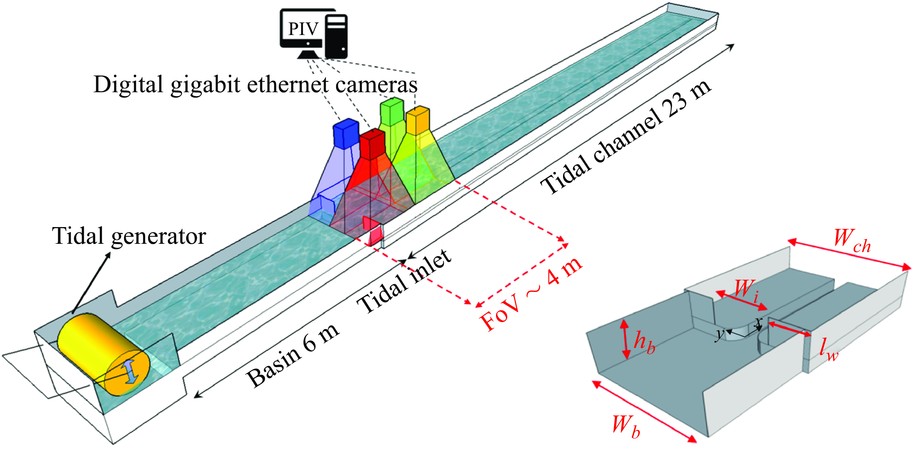
Figure 1. Sketch of the experimental tidal flume and the image acquisition system. The inset shows a close-up of the field of view (FoV).
The laboratory flume (figure 1) consists of two main components: a compound tidal channel that is 23 m long and 2.5 m wide, and a rectangular basin representing open sea conditions, approximately 6 m long, 2.2 m wide and 0.5 m deep. This latter depth is denoted by $h_{b}$
in the inset of figure 1, whereas the channel and the basin widths are marked by
$h_{b}$
in the inset of figure 1, whereas the channel and the basin widths are marked by $w_{ch}$
and
$w_{ch}$
and $w_{b}$
, respectively. The basin is connected to the tidal channel through an inlet made of two vertical barriers, whose length
$w_{b}$
, respectively. The basin is connected to the tidal channel through an inlet made of two vertical barriers, whose length $l_w$
is 0.86 m. The net inlet entrance width
$l_w$
is 0.86 m. The net inlet entrance width $w_i$
is 0.7 m. The channel has a symmetric composite transversal profile with a deep main channel and wide lateral tidal flats.
$w_i$
is 0.7 m. The channel has a symmetric composite transversal profile with a deep main channel and wide lateral tidal flats.
A volume wave generator, located at the end of the basin, generates the periodic tidal wave following a monochromatic wave with a time law of the type $\eta (t)=a\sin {({2\pi \! t}/{T})}$
, where
$\eta (t)=a\sin {({2\pi \! t}/{T})}$
, where $\eta$
is the free surface elevation,
$\eta$
is the free surface elevation, $a$
is the tidal amplitude,
$a$
is the tidal amplitude, $T$
is the tidal period, and
$T$
is the tidal period, and $t$
is the time.
$t$
is the time.
For the present experiments, we kept the mean water level at the channel inlet ( $D_0$
) and the tidal wave period constant at 0.12 m and 100 s, respectively. Consequently, the inviscid tidal wavelength
$D_0$
) and the tidal wave period constant at 0.12 m and 100 s, respectively. Consequently, the inviscid tidal wavelength $L_g=T\sqrt {g D_0}$
was also kept constant. In table 1, we reported the main parameters of the experiments together with the estimate of the Reynolds number defined as
$L_g=T\sqrt {g D_0}$
was also kept constant. In table 1, we reported the main parameters of the experiments together with the estimate of the Reynolds number defined as $R_e = U \mathcal{L} / \nu$
, where
$R_e = U \mathcal{L} / \nu$
, where $U$
is the maximum velocity registered at the tidal inlet,
$U$
is the maximum velocity registered at the tidal inlet, $\nu$
is the kinematic fluid viscosity, and
$\nu$
is the kinematic fluid viscosity, and $\mathcal{L}$
is an integral length scale, set equal to the length of the inlet barrier
$\mathcal{L}$
is an integral length scale, set equal to the length of the inlet barrier $l_w$
, consistent with previous work by De Leo & Stocchino (2022). This choice of scales for the characteristic Reynolds number is determined by the fact that the surface turbulence is expected to be driven primarily by the shedding of large-scale vortices generated by the interaction between the tide and the inlet barriers in a jet-like shape.
$l_w$
, consistent with previous work by De Leo & Stocchino (2022). This choice of scales for the characteristic Reynolds number is determined by the fact that the surface turbulence is expected to be driven primarily by the shedding of large-scale vortices generated by the interaction between the tide and the inlet barriers in a jet-like shape.
Table 1. Main experimental parameters: $T$
is the tidal period,
$T$
is the tidal period, $U$
is the maximum velocity registered at the tidal inlet,
$U$
is the maximum velocity registered at the tidal inlet, $\epsilon =a/D_0$
is the non-dimensional tidal amplitude, where
$\epsilon =a/D_0$
is the non-dimensional tidal amplitude, where $a$
is the amplitude and
$a$
is the amplitude and $D_0$
is the mean water level,
$D_0$
is the mean water level, $R_e$
is the Reynolds number,
$R_e$
is the Reynolds number, $L_g$
is the inviscid tidal wavelength, and
$L_g$
is the inviscid tidal wavelength, and $\eta _k$
and
$\eta _k$
and $u_{\eta }$
are the Kolmogorov length and velocity scale, respectively.
$u_{\eta }$
are the Kolmogorov length and velocity scale, respectively.

Based on the above large length and velocity scales, we also evaluated the Kolmogorov length scale as $\eta _k = l_w\, Re^{-3/4}$
and the associated velocity scale as
$\eta _k = l_w\, Re^{-3/4}$
and the associated velocity scale as $u_{\eta }=\nu /\eta _k$
(Tennekes & Lumley Reference Tennekes and Lumley1972). The Kolmogorov scales are used in the following to characterise the fibres and to provide dimensionless values of key variables, namely the flow and fibre structure functions.
$u_{\eta }=\nu /\eta _k$
(Tennekes & Lumley Reference Tennekes and Lumley1972). The Kolmogorov scales are used in the following to characterise the fibres and to provide dimensionless values of key variables, namely the flow and fibre structure functions.
2.2. Fibre characterisation and Stokes numbers estimation
In this work, we investigated three different classes of rigid fibre-like dipoles, consisting of two small polystyrene spheres (radius 5 mm) connected together with a rigid wooden rod of 1 mm diameter. The three classes of fibres, labelled Class 01, Class 02 and Class 03, had centre-to-centre lengths 40, 60 and 90 mm, respectively, with error $\pm$
1 mm, and they were released into the flow with a random orientation distribution, with starting point placed always outside the field of view (FoV); see figure 1. Moreover, the dispersed fibres always float on the water surface remaining on the
$\pm$
1 mm, and they were released into the flow with a random orientation distribution, with starting point placed always outside the field of view (FoV); see figure 1. Moreover, the dispersed fibres always float on the water surface remaining on the $x{-}y$
plane.
$x{-}y$
plane.
For the present analysis, it is important to ensure negligible rotational inertia, which means having the fibre rotational Stokes number $S_t$
much smaller than unity. In general,
$S_t$
much smaller than unity. In general, $S_t$
is defined as the ratio between the relaxation time of the fibre (
$S_t$
is defined as the ratio between the relaxation time of the fibre ( $\tau _p$
) and a typical time scale of the flow (
$\tau _p$
) and a typical time scale of the flow ( $\tau _f$
), i.e.
$\tau _f$
), i.e. $S_t = \tau _p/\tau _f$
. As far as
$S_t = \tau _p/\tau _f$
. As far as $\tau _f$
is concerned, a natural choice when dealing with tidal flows is the tidal wave period
$\tau _f$
is concerned, a natural choice when dealing with tidal flows is the tidal wave period $T$
(Toffolon et al. Reference Toffolon, Vignoli and Tubino2006; Cai et al. Reference Cai, Savenije and Toffolon2012).
$T$
(Toffolon et al. Reference Toffolon, Vignoli and Tubino2006; Cai et al. Reference Cai, Savenije and Toffolon2012).
To estimate $S_t$
, we first convert the geometry of our rigid fibre into an equivalent prolate spheroid; see Voth & Soldati (Reference Voth and Soldati2017). In particular, we assumed that the area originally occupied by the fibre would be redistributed over the surface of an equivalent prolate spheroid in such a way that its major axis corresponded to the length of the fibre,
$S_t$
, we first convert the geometry of our rigid fibre into an equivalent prolate spheroid; see Voth & Soldati (Reference Voth and Soldati2017). In particular, we assumed that the area originally occupied by the fibre would be redistributed over the surface of an equivalent prolate spheroid in such a way that its major axis corresponded to the length of the fibre, $L$
. From the equivalence of the areas, the evaluation of the minor axis of the spheroid
$L$
. From the equivalence of the areas, the evaluation of the minor axis of the spheroid $B$
is straightforward. Once the dimensions of the spheroid are known, we can define the aspect ratio
$B$
is straightforward. Once the dimensions of the spheroid are known, we can define the aspect ratio $\lambda$
as the ratio of the major axis to the minor axis,
$\lambda$
as the ratio of the major axis to the minor axis, $\lambda =L/B$
.
$\lambda =L/B$
.
Then two distinct approaches to estimate $S_t$
are adopted. The first approach consists in employing the relationship proposed by Shapiro & Goldenberg (Reference Shapiro and Goldenberg1993), Zhao et al. (Reference Zhao, Challabotla, Andersson and Variano2015) and Voth & Soldati (Reference Voth and Soldati2017), which reads
$S_t$
are adopted. The first approach consists in employing the relationship proposed by Shapiro & Goldenberg (Reference Shapiro and Goldenberg1993), Zhao et al. (Reference Zhao, Challabotla, Andersson and Variano2015) and Voth & Soldati (Reference Voth and Soldati2017), which reads
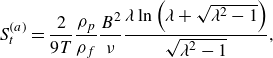 \begin{equation} S_t^{(a)} = \frac {2}{9T} \frac {\rho _p}{\rho _f} \frac {B^2}{\nu } \frac {\lambda \ln \left (\lambda +\sqrt {\lambda ^2-1}\right )}{\sqrt {\lambda ^2-1}} \textrm {,} \end{equation}
where $T$
is the tidal period,
$T$
is the tidal period, $\rho _p=900\,\textrm kg\, \textrm{m}^{-3}$
and
$\rho _p=900\,\textrm kg\, \textrm{m}^{-3}$
and $\rho _f=1000\,\textrm kg\,\textrm{m}^-{^3}$
are the fibre and fluid densities, respectively,
$\rho _f=1000\,\textrm kg\,\textrm{m}^-{^3}$
are the fibre and fluid densities, respectively, $B$
is the minor axis,
$B$
is the minor axis, $\lambda$
is the aspect ratio of the equivalent prolate spheroid, and
$\lambda$
is the aspect ratio of the equivalent prolate spheroid, and $\nu$
is the kinematic fluid viscosity (
$\nu$
is the kinematic fluid viscosity ( $10^{-6}\,\textrm m^{2}\, \textrm{s}^{-1}$
).
$10^{-6}\,\textrm m^{2}\, \textrm{s}^{-1}$
).
The second approach estimates the Stokes number by means of the fibre rotational relaxation time using the formulation by Bounoua et al. (Reference Bounoua, Bouchet and Verhille2018) as
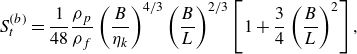 \begin{equation} S_t^{(b)} = \frac {1}{48} \frac {\rho _p}{\rho _f}\left (\frac {B}{\eta _k}\right )^{4 / 3}\left (\frac {B}{L}\right )^{2 / 3}\left [1+\frac {3}{4}\left (\frac {B}{L}\right )^2\right ] \textrm {,} \end{equation}
where $\eta _k$
is the Kolmogorov length (Kolmogorov Reference Kolmogorov1941a
,Reference Kolmogorov
b
) and
$\eta _k$
is the Kolmogorov length (Kolmogorov Reference Kolmogorov1941a
,Reference Kolmogorov
b
) and $L$
is the centre-to-centre pole distance as in table 2.
$L$
is the centre-to-centre pole distance as in table 2.
Table 2. Main fibre parameters: $L$
is the fibre length,
$L$
is the fibre length, $\lambda$
is the aspect ratio of the equivalent prolate spheroid, and
$\lambda$
is the aspect ratio of the equivalent prolate spheroid, and $S_t$
is the Stokes number. The superscripts (a) and (b) indicate
$S_t$
is the Stokes number. The superscripts (a) and (b) indicate $S_t$
computed with (2.1) and (2.2), respectively.
$S_t$
computed with (2.1) and (2.2), respectively.
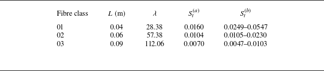
Note that neither (2.1) nor (2.2) is strictly applicable to the present case. On the one hand, (2.1) is valid only for infinitesimal particles, which is not the case in our experiments. On the other hand, (2.2) is derived under the assumption that the fibre tumbling is a Langevin process driven by a random delta-correlated-in-time forcing, whose variance is set by using Kolmogorov scaling for the velocity differences. This hypothesis is, in principle, not valid for non-ideal turbulence. Nevertheless, both (2.1) and (2.2) can be used to estimate the order of magnitude of $S_t$
. The results of the different approaches for Stokes numbers, the values of the fibre slenderness
$S_t$
. The results of the different approaches for Stokes numbers, the values of the fibre slenderness $\lambda$
, and the Kolmogorov scales are reported in table 2 for comparison. In all cases, the Stokes number of the fibres considered is much smaller than unity, i.e. the fibre response time is instantaneous.
$\lambda$
, and the Kolmogorov scales are reported in table 2 for comparison. In all cases, the Stokes number of the fibres considered is much smaller than unity, i.e. the fibre response time is instantaneous.
2.3. Eulerian flow measurements and fibre tracking algorithm
In the present experiments, we simultaneously measured the fluid Eulerian velocity fields and the fibre trajectories. In particular, the two-dimensional time-resolved Eulerian free surface velocity ( $\boldsymbol{u}(\boldsymbol{x},t)=(u(\boldsymbol{x},t),v(\boldsymbol{x},t))$
) was measured using the same PIV set-up employed in previous studies (De Leo & Stocchino 2022; De Leo et al. Reference De Leo, Enrile and Stocchino2022a
,
Reference De Leo, Tambroni and Stocchinob
). Note that the origin of the coordinate system,
$\boldsymbol{u}(\boldsymbol{x},t)=(u(\boldsymbol{x},t),v(\boldsymbol{x},t))$
) was measured using the same PIV set-up employed in previous studies (De Leo & Stocchino 2022; De Leo et al. Reference De Leo, Enrile and Stocchino2022a
,
Reference De Leo, Tambroni and Stocchinob
). Note that the origin of the coordinate system, $\boldsymbol{x}=(x,y)$
, was placed at the inlet opening in the middle of the channel, with the
$\boldsymbol{x}=(x,y)$
, was placed at the inlet opening in the middle of the channel, with the $x$
-axis pointing towards the end of the main channel, and the
$x$
-axis pointing towards the end of the main channel, and the $y$
-axis following the right-hand rule.
$y$
-axis following the right-hand rule.
Regarding the PIV, the acquisition system consisted of four digital cameras (Teledyne Dalsa Genie Nano 89 C1280, resolution 1280 $\times$
1024 pixels) placed on the tidal flume pointing downward to the free surface and covering a FoV of approximately 4 m times 2.5 m (the entire flume width), see figure 1 for reference. The images recorded separately by the four cameras, at a frequency of 15 fps, were merged together before the PIV analysis, which was performed using the software proVision-XS (Integrated Design Tools (IDT), Inc.). The final spatial resolution of the measured velocity fields was approximately one vector every 31 mm in both
$\times$
1024 pixels) placed on the tidal flume pointing downward to the free surface and covering a FoV of approximately 4 m times 2.5 m (the entire flume width), see figure 1 for reference. The images recorded separately by the four cameras, at a frequency of 15 fps, were merged together before the PIV analysis, which was performed using the software proVision-XS (Integrated Design Tools (IDT), Inc.). The final spatial resolution of the measured velocity fields was approximately one vector every 31 mm in both $x$
and
$x$
and $y$
directions. It is worth noting that fibres released during the experiments did not significantly influence the Eulerian velocities at the scale resolved by the PIV. This is reasonable to expect since the fibre mass fraction used in the present experiments is extremely low, and it has been shown that only at very high fibre concentration the flow is influenced by the presence of the fibres (Olivieri et al. Reference Olivieri, Mazzino and Rosti2022). However, to test this assumption, we repeated experiment 4 twice without the fibres using the same forcing conditions (tidal amplitude and period) and then compared the time averaged velocity fields in terms of single velocity components and of the velocity module. The percentage differences between the two repetitions without fibres were 0.09
$y$
directions. It is worth noting that fibres released during the experiments did not significantly influence the Eulerian velocities at the scale resolved by the PIV. This is reasonable to expect since the fibre mass fraction used in the present experiments is extremely low, and it has been shown that only at very high fibre concentration the flow is influenced by the presence of the fibres (Olivieri et al. Reference Olivieri, Mazzino and Rosti2022). However, to test this assumption, we repeated experiment 4 twice without the fibres using the same forcing conditions (tidal amplitude and period) and then compared the time averaged velocity fields in terms of single velocity components and of the velocity module. The percentage differences between the two repetitions without fibres were 0.09 $\pm$
0.65 % and −0.09
$\pm$
0.65 % and −0.09 $\pm$
0.66 % for
$\pm$
0.66 % for $u(\boldsymbol{x},t)$
and
$u(\boldsymbol{x},t)$
and $v(\boldsymbol{x},t)$
, respectively, and 0.55
$v(\boldsymbol{x},t)$
, respectively, and 0.55 $\pm$
0.78 % for the velocity modulus. The differences observed between the experiments with and without fibres lead to values 0.1
$\pm$
0.78 % for the velocity modulus. The differences observed between the experiments with and without fibres lead to values 0.1 $\pm$
0.7 %, −0.08
$\pm$
0.7 %, −0.08 $\pm$
0.56 % and 0.5
$\pm$
0.56 % and 0.5 $\pm$
0.75 % for the velocity components and modulus, respectively. Differences of the order of 1
$\pm$
0.75 % for the velocity components and modulus, respectively. Differences of the order of 1 $\%$
are within the expected repeatability of the experiments, and the presence of the fibres did not produce statistically significant differences.
$\%$
are within the expected repeatability of the experiments, and the presence of the fibres did not produce statistically significant differences.
Regarding the fibre tracking algorithm, we employed a novel two-step framework for multi-object tracing, enabling precise detection and tracking of both fibres and their poles within frame sequences. Given a sequence of frames $\mathcal{V} = \{v_{1}, \ldots, v_{t}, \ldots, v_{T}\}$
, where
$\mathcal{V} = \{v_{1}, \ldots, v_{t}, \ldots, v_{T}\}$
, where $v_{t}$
represented the
$v_{t}$
represented the $t$
th frame, we identified
$t$
th frame, we identified $K$
distinct fibres, depicted as
$K$
distinct fibres, depicted as $\boldsymbol{d}_t = \{{d}_t^1, \ldots, {d}_t^k, \ldots, {d}_t^K\}$
, where
$\boldsymbol{d}_t = \{{d}_t^1, \ldots, {d}_t^k, \ldots, {d}_t^K\}$
, where $d_t^k$
denoted the
$d_t^k$
denoted the $k$
th fibre. Each fibre
$k$
th fibre. Each fibre ${d}_t^k$
was characterised by a tuple
${d}_t^k$
was characterised by a tuple $(\text{fibre\_id}, x_1^k, y_1^k, x_2^k, y_2^k)$
, wherein
$(\text{fibre\_id}, x_1^k, y_1^k, x_2^k, y_2^k)$
, wherein $\text{fibre\_id}$
was a unique identifier that persisted across frames for tracking continuity. The tuple elements
$\text{fibre\_id}$
was a unique identifier that persisted across frames for tracking continuity. The tuple elements $x_1^k, y_1^k$
and
$x_1^k, y_1^k$
and $x_2^k, y_2^k$
corresponded to the pixel coordinates of the fibre’s poles. Our objective was to establish
$x_2^k, y_2^k$
corresponded to the pixel coordinates of the fibre’s poles. Our objective was to establish $\boldsymbol{d}_t$
for each frame
$\boldsymbol{d}_t$
for each frame $v_t$
, allowing for the detection of pole trajectories throughout the sequence of recorded frames.
$v_t$
, allowing for the detection of pole trajectories throughout the sequence of recorded frames.

In the initial phase, our approach used two YOLOv8-based deep detectors to locate fibres and their corresponding poles (Li et al. Reference Li, Fan, Huang, Han and Gu2023; Talaat & ZainEldin Reference Talaat and ZainEldin2023). The algorithm started by pinpointing fibres, from which it cropped the relevant image regions for the subsequent step to determine the exact positions of the poles.
The framework then moved into its second phase, focusing on the consistent identification of each fibre and pole across frames. We introduced a pair of measures to determine the distance between objects, namely the Euclidean distance and the Intersection over Union (IoU), an unsupervised tracking algorithm inspired by Bochinski et al. (Reference Bochinski, Eiselein and Sikora2017). The main assumption was that the nearest object in the following frame was recognised as the subsequent position of the current object.
Given two bounding boxes of two objects $ A_i$
and
$ A_i$
and $ B_j$
, the IoU is calculated as
$ B_j$
, the IoU is calculated as
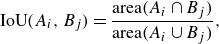 \begin{equation} \text{IoU}(A_i, B_j) = \frac {\text{area}(A_i \cap B_j)}{\text{area}(A_i \cup B_j)}, \end{equation}
where $ \text{area}(A_i \cap B_j)$
was the area of the intersection, and
$ \text{area}(A_i \cap B_j)$
was the area of the intersection, and $ \text{area}(A_i \cup B_j)$
was the area of the union of the two bounding boxes.
$ \text{area}(A_i \cup B_j)$
was the area of the union of the two bounding boxes.
Let $ (x_i, y_i)$
and
$ (x_i, y_i)$
and $ (x_j, y_j)$
be the centre coordinates of poles
$ (x_j, y_j)$
be the centre coordinates of poles $ A_i$
and
$ A_i$
and $ B_j$
, respectively. Then the Euclidean distance between them could be calculated as
$ B_j$
, respectively. Then the Euclidean distance between them could be calculated as
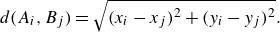 \begin{equation} d(A_i, B_j) = \sqrt {(x_i - x_j)^2 + (y_i - y_j)^2}. \end{equation}
The novel contribution of our algorithm lies in the implementation of a hierarchical detection and tracking scheme. We adopted an IoU-based continuity criterion for fibres, which served as a robust metric for preserving track continuity across consecutive frames. In contrast, for poles, where the regions of interest were significantly smaller, we used the Euclidean distance as the tracking metric. The detailed workflow is illustrated in algorithm1 through a pseudo-code.
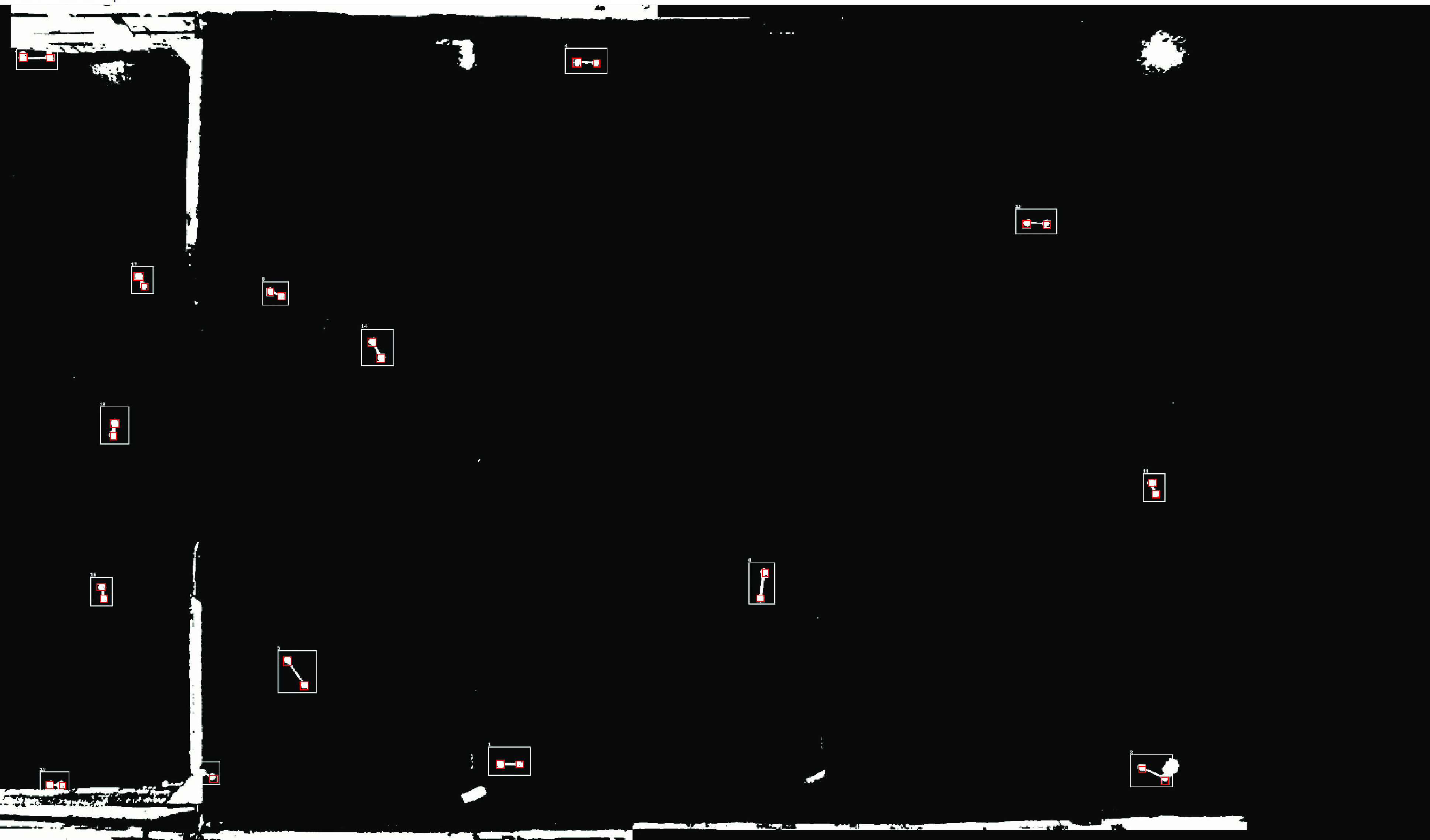
Figure 2. Example of the new tracking algorithm applied to one frame of experiment 1. A threshold has been applied to the original recorded images before tracking the fibres to remove the PIV seeding particles and improve contrast between the fibre and the background. The code automatically detects and tracks fibres (white boxes) as well as lateral poles (red boxes) within image sequences. This frame was taken during a tidal flood phase, flow from left to right.
Figure 2 shows a snapshot of the application of the proposed tracking algorithm. The image represents one frame from experiment 1 of the surveyed region. As a result of the threshold applied to the original image to remove PIV particle seeding and improve contrast with the fibre, the background is almost completely black. On the left is still visible, in white, the tidal barrier that divides the basin (left-hand side) from the tidal channel (right-hand side). The fibres are clearly visible surrounded by the rectangular bounding boxes, automatically identified and tracked by the algorithm. In each frame, all three fibre classes are, on average, always found. Moreover, the density of fibres in the FoV shown in figure 2 is the typical density maintained during all the experiments.
The number of tracked fibres during the four experiments ranged between $50$
(for experiment 1) to
$50$
(for experiment 1) to $121$
(for experiment 4), with a trajectory time duration between
$121$
(for experiment 4), with a trajectory time duration between $10\,{\textrm s}$
and
$10\,{\textrm s}$
and $620\,{\textrm s}$
. The wide range of durations observed depended on the initial seeding location of the fibres and the background Eulerian velocities. Note that the FoV of the acquisition system did not cover the full length of the flume, thus cases where a fibre entered or exited the measurement area were unavoidable. However, this issue did not substantially influence the results of the analysis. Indeed, most of the trajectories lasted for more than a single tidal period of 100 s, in some cases reaching up to six consecutive periods. Moreover, the trajectories were almost equally distributed among the three Classes of fibres. In all experiments, the algorithm detected a total number of objects classified as Class 01, 02 and 03 fibres equal to
$620\,{\textrm s}$
. The wide range of durations observed depended on the initial seeding location of the fibres and the background Eulerian velocities. Note that the FoV of the acquisition system did not cover the full length of the flume, thus cases where a fibre entered or exited the measurement area were unavoidable. However, this issue did not substantially influence the results of the analysis. Indeed, most of the trajectories lasted for more than a single tidal period of 100 s, in some cases reaching up to six consecutive periods. Moreover, the trajectories were almost equally distributed among the three Classes of fibres. In all experiments, the algorithm detected a total number of objects classified as Class 01, 02 and 03 fibres equal to $143\,854$
,
$143\,854$
, $137\,740$
and
$137\,740$
and $119\,277$
, respectively. The average estimated centre-to-centre distances for the three classes were 35.7
$119\,277$
, respectively. The average estimated centre-to-centre distances for the three classes were 35.7 $\pm$
1.7 mm, 58.7
$\pm$
1.7 mm, 58.7 $\pm$
2.3 mm and 86.1
$\pm$
2.3 mm and 86.1 $\pm$
3.1 mm, demonstrating the good accuracy of the tracking algorithm. Note that the obtained standard deviation corresponded to 1 or 2 pixels, with a single pixel equal to 1.6 mm.
$\pm$
3.1 mm, demonstrating the good accuracy of the tracking algorithm. Note that the obtained standard deviation corresponded to 1 or 2 pixels, with a single pixel equal to 1.6 mm.
The final outputs of the fibre tracking algorithm are the positions in time of the two poles of the fibre, denoted as $\boldsymbol{X}_A$
and
$\boldsymbol{X}_A$
and $\boldsymbol{X}_B$
, and of its centre of mass
$\boldsymbol{X}_B$
, and of its centre of mass $\boldsymbol{X}_c$
. From the position in time, we evaluated the Lagrangian velocities
$\boldsymbol{X}_c$
. From the position in time, we evaluated the Lagrangian velocities $\boldsymbol{V}^A(t)$
,
$\boldsymbol{V}^A(t)$
, $\boldsymbol{V}^B(t)$
and
$\boldsymbol{V}^B(t)$
and $\boldsymbol{V}^c(t)$
, respectively, along the trajectories.
$\boldsymbol{V}^c(t)$
, respectively, along the trajectories.
2.4. Description of the fibre motion
We aim to investigate how the fibre dynamics is coupled with the background Eulerian flow, and in particular, how the Eulerian fluid velocities at the same positions as the fibre poles, usually called the fluid seen-by-particle velocities (Jung et al. Reference Jung, Yeo and Lee2008), drive the fibre rotation. To this end, we first evaluate the Eulerian velocity in the positions experienced by the fibre trajectories by interpolating the PIV field ( $\boldsymbol{u}(\boldsymbol{x},t)$
) at the pole positions (
$\boldsymbol{u}(\boldsymbol{x},t)$
) at the pole positions ( $\boldsymbol{X}_A(t)$
,
$\boldsymbol{X}_A(t)$
, $\boldsymbol{X}_B(t)$
) and at the fibre centre of mass (
$\boldsymbol{X}_B(t)$
) and at the fibre centre of mass ( $\boldsymbol{X}_C(t)$
) using a bi-cubic interpolation algorithm. Once the Lagrangian fibre velocities (
$\boldsymbol{X}_C(t)$
) using a bi-cubic interpolation algorithm. Once the Lagrangian fibre velocities ( $\boldsymbol{V}_A(t)$
,
$\boldsymbol{V}_A(t)$
, $\boldsymbol{V}_B(t)$
) and fluid seen-by-particle Eulerian velocities (
$\boldsymbol{V}_B(t)$
) and fluid seen-by-particle Eulerian velocities ( $\boldsymbol{u}_A(t)$
,
$\boldsymbol{u}_A(t)$
, $\boldsymbol{u}_B(t)$
) are known, we compute
$\boldsymbol{u}_B(t)$
) are known, we compute
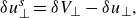
 \begin{equation} \delta \boldsymbol{V}=\boldsymbol{V}_{B}-\boldsymbol{V}_{A}, \quad \delta \boldsymbol{u}=\boldsymbol{u}_{B}-\boldsymbol{u}_{A}, \end{equation}
where $\delta \boldsymbol{V}$
and
$\delta \boldsymbol{V}$
and $\delta \boldsymbol{u}$
are the Lagrangian and Eulerian velocity differences between the fibre endpoints, respectively.
$\delta \boldsymbol{u}$
are the Lagrangian and Eulerian velocity differences between the fibre endpoints, respectively.
From (2.5), we then compute the transverse components, namely projection along the unit vector normal orthogonal to the fibre axis ( $\hat {\boldsymbol{r}}_{\bot }$
), as (Cavaiola et al. Reference Cavaiola, Olivieri and Mazzino2020)
$\hat {\boldsymbol{r}}_{\bot }$
), as (Cavaiola et al. Reference Cavaiola, Olivieri and Mazzino2020)
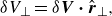 \begin{align} \delta V_{\bot }=\delta \boldsymbol{V} \boldsymbol{\cdot } \hat {\boldsymbol{r}}_{\bot }, \end{align}
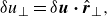 \begin{align} \delta u_{\bot }=\delta \boldsymbol{u} \boldsymbol{\cdot } \hat {\boldsymbol{r}}_{\bot }, \end{align}
where $\delta V_{\bot }$
is the Lagrangian projected velocity of the fibre, and
$\delta V_{\bot }$
is the Lagrangian projected velocity of the fibre, and $\delta u_{\bot }$
is the Eulerian projected velocity seen by fibre. The transverse velocity differences are indeed the only component responsible for the fibre rotation. Specifically, the Lagrangian velocity difference between the fibre endpoints is related to the variation of the fibre’s axis rotation per unit time, as this equals
$\delta u_{\bot }$
is the Eulerian projected velocity seen by fibre. The transverse velocity differences are indeed the only component responsible for the fibre rotation. Specifically, the Lagrangian velocity difference between the fibre endpoints is related to the variation of the fibre’s axis rotation per unit time, as this equals $\delta V_{\perp }/L$
. Generally, the Lagrangian and Eulerian transverse velocity differences are of the same order of magnitude (
$\delta V_{\perp }/L$
. Generally, the Lagrangian and Eulerian transverse velocity differences are of the same order of magnitude ( $\delta V_{\perp } \sim \delta u_{\perp }$
), as the fibre rotates preferentially due to the interaction with the eddies of its own size (Parsa & Voth Reference Parsa and Voth2014; Bounoua et al. Reference Bounoua, Bouchet and Verhille2018; Brizzolara et al. Reference Brizzolara, Rosti, Olivieri, Brandt, Holzner and Mazzino2021). This phenomenon is referred to as scale selection.
$\delta V_{\perp } \sim \delta u_{\perp }$
), as the fibre rotates preferentially due to the interaction with the eddies of its own size (Parsa & Voth Reference Parsa and Voth2014; Bounoua et al. Reference Bounoua, Bouchet and Verhille2018; Brizzolara et al. Reference Brizzolara, Rosti, Olivieri, Brandt, Holzner and Mazzino2021). This phenomenon is referred to as scale selection.
Note that if the fibre moves on a plane, then the projection of the velocity difference of (2.5) along the direction parallel to the fibre would simply lead to zero, as the fibre is rigid and inextensible in the present case (Cavaiola et al. Reference Cavaiola, Olivieri and Mazzino2020).
Different properties of the transverse velocity differences (2.6) and (2.7) can be analysed. First, a one-to-one comparison of the instantaneous signal is useful to understand how the fibres drift with the background flow. Second, we can define a rotational slip velocity as
 \begin{equation} \delta u_{\bot }^{s} = \delta V_{\bot } - \delta u_{\bot } \textrm {,} \end{equation}
which quantifies to what extent the Lagrangian projected velocity differs from the Eulerian signal instantaneously.
The properties of $\delta V_{\bot }$
and
$\delta V_{\bot }$
and $\delta u_{\bot }$
can be further characterised by their statistical properties, from the probability distribution function to the statistical moments, i.e. the structure functions. In particular, we focus on the scaling of the second- and third-order moments of
$\delta u_{\bot }$
can be further characterised by their statistical properties, from the probability distribution function to the statistical moments, i.e. the structure functions. In particular, we focus on the scaling of the second- and third-order moments of $|\delta V_{\bot }|$
, which are the FTV-based absolute value transverse structure functions (Brizzolara et al. Reference Brizzolara, Rosti, Olivieri, Brandt, Holzner and Mazzino2021)
$|\delta V_{\bot }|$
, which are the FTV-based absolute value transverse structure functions (Brizzolara et al. Reference Brizzolara, Rosti, Olivieri, Brandt, Holzner and Mazzino2021)
 \begin{equation} S_2^{\bot } = \langle {\delta V_{\bot }}^2 \rangle, \quad S_3^{\bot } = \langle {|\delta V_{\bot }|}^3 \rangle \textrm {,} \end{equation}
where $\langle \cdot \rangle$
indicates the average over all the fibre trajectories belonging to the same class length and flow Reynolds number in space and time. We preferred to use the relative third-order structure function (Arneodo et al. Reference Arneodo1996) due to the periodicity of the Eulerian mean flow, which induces a periodic reversal of the main longitudinal velocity.
$\langle \cdot \rangle$
indicates the average over all the fibre trajectories belonging to the same class length and flow Reynolds number in space and time. We preferred to use the relative third-order structure function (Arneodo et al. Reference Arneodo1996) due to the periodicity of the Eulerian mean flow, which induces a periodic reversal of the main longitudinal velocity.
3. Results and discussion
3.1. The background Eulerian turbulent tidal flow
The description of the flow under investigation encompasses both Eulerian and Lagrangian properties, and for details we refer the reader to De Leo et al. (Reference De Leo, Tambroni and Stocchino2022b ). In the following paragraphs, we will briefly summarise the main features, which we believe will be helpful in discussing the present results.
The volume wave arising from the periodic oscillation of the tidal generator propagates towards the tidal channel with wavelength $L_g$
much longer than the channel length, avoiding resonant behaviours of the tidal waves (Garrett Reference Garrett1972; Savenije Reference Savenije2001). Subsequently, the resulting flow remains relatively regular until it encounters the tidal inlet during the flood phase, i.e. when the mean flow intrudes into the tidal channel. As soon as the almost uniform flow reaches the lateral inlet barriers, vortex shedding is observed at the tips of the two plates of length
$L_g$
much longer than the channel length, avoiding resonant behaviours of the tidal waves (Garrett Reference Garrett1972; Savenije Reference Savenije2001). Subsequently, the resulting flow remains relatively regular until it encounters the tidal inlet during the flood phase, i.e. when the mean flow intrudes into the tidal channel. As soon as the almost uniform flow reaches the lateral inlet barriers, vortex shedding is observed at the tips of the two plates of length $l_w$
. During the flood phase, a series of small-scale vortices is continuously emitted and merged into a larger recirculating structure occupying the entire lateral flat, as observed previously by Nicolau del Roure et al. (2009). Recently, this process has been reinterpreted by De Leo et al. (Reference De Leo, Enrile and Stocchino2022a
) through the use of Lagrangian-Averaged Vorticity Deviation (LAVD) (Haller et al. Reference Haller, Hadjighasem, Farazmand and Huhn2016) and Finite Time Lyapunov Exponent (FTLE) dynamics (Haller Reference Haller2015), which showed the entrainment of small-scale vortices within the main vortical structure. In particular, detailed analysis of the LAVD dynamics demonstrated the occurrence of a clear vortex thinning mechanism (Chen et al. Reference Chen, Ecke, Eyink, Rivera, Wan and Xiao2006), ultimately linked to an inverse energy cascade (De Leo & Stocchino 2022).
$l_w$
. During the flood phase, a series of small-scale vortices is continuously emitted and merged into a larger recirculating structure occupying the entire lateral flat, as observed previously by Nicolau del Roure et al. (2009). Recently, this process has been reinterpreted by De Leo et al. (Reference De Leo, Enrile and Stocchino2022a
) through the use of Lagrangian-Averaged Vorticity Deviation (LAVD) (Haller et al. Reference Haller, Hadjighasem, Farazmand and Huhn2016) and Finite Time Lyapunov Exponent (FTLE) dynamics (Haller Reference Haller2015), which showed the entrainment of small-scale vortices within the main vortical structure. In particular, detailed analysis of the LAVD dynamics demonstrated the occurrence of a clear vortex thinning mechanism (Chen et al. Reference Chen, Ecke, Eyink, Rivera, Wan and Xiao2006), ultimately linked to an inverse energy cascade (De Leo & Stocchino 2022).
During the ebb phase of the tide, an inversion of the mean flow occurs, with the main flow directed towards the outer basin. This results in the disruption of the large gyres, with the subsequent large-scale flow carrying the macro-vortices out of the tidal channel. The observed asymmetry between the vortex shedding at the inlet during the flood and ebb phase, and the resulting ebb dominance (De Leo et al. Reference De Leo, Tambroni and Stocchino2022b
), can be attributed to two main factors: the geometry of the channel (compound cross-section) and the geometry of the basin (rectangular cross-section). In contrast, the symmetry of the inlet and tidal channel geometries with respect to the $x$
-axis implies the existence of symmetry in the flow along the transverse direction.
$x$
-axis implies the existence of symmetry in the flow along the transverse direction.
If we now consider the phase-averaged velocity fields, also known as residual tidal currents (Jay Reference Jay1991), then De Leo et al. (Reference De Leo, Tambroni and Stocchino2022b
) showed how the pattern of the averaged velocity fields depends on the main tidal parameters (amplitude $\epsilon$
, period
$\epsilon$
, period $T$
and tidal shape factor). In the present case, we decided to keep the tidal period constant and vary only the amplitude. Figure 3 shows two examples of the residual currents observed in the present experiments, i.e. experiment 1, with the minimum
$T$
and tidal shape factor). In the present case, we decided to keep the tidal period constant and vary only the amplitude. Figure 3 shows two examples of the residual currents observed in the present experiments, i.e. experiment 1, with the minimum $\epsilon$
(figure 3
a), and experiment 4, with the maximum
$\epsilon$
(figure 3
a), and experiment 4, with the maximum $\epsilon$
(figure 3
b). As expected, increasing the tidal amplitude generates two symmetric longer gyres downstream of the tidal inlet, whose width is controlled and limited by the transverse extension of the later floodplains.
$\epsilon$
(figure 3
b). As expected, increasing the tidal amplitude generates two symmetric longer gyres downstream of the tidal inlet, whose width is controlled and limited by the transverse extension of the later floodplains.

Figure 3. Example of residual velocity fields: (a) experiment 1 ( $\epsilon =0.0082$
,
$\epsilon =0.0082$
, $T=100$
s), and (b) experiment 4 (
$T=100$
s), and (b) experiment 4 ( $\epsilon =0.0258$
,
$\epsilon =0.0258$
, $T=100$
s).
$T=100$
s).

Figure 4. All recorded fibre trajectories for the four experiments: (a) experiment 1, (b) experiment 2, (c) experiment 3, (d) experiment 4. Different colours identify different fibre classes: class 01 in black; class 02 in light blue; class 03 in pink.
3.2. Fibre trajectories
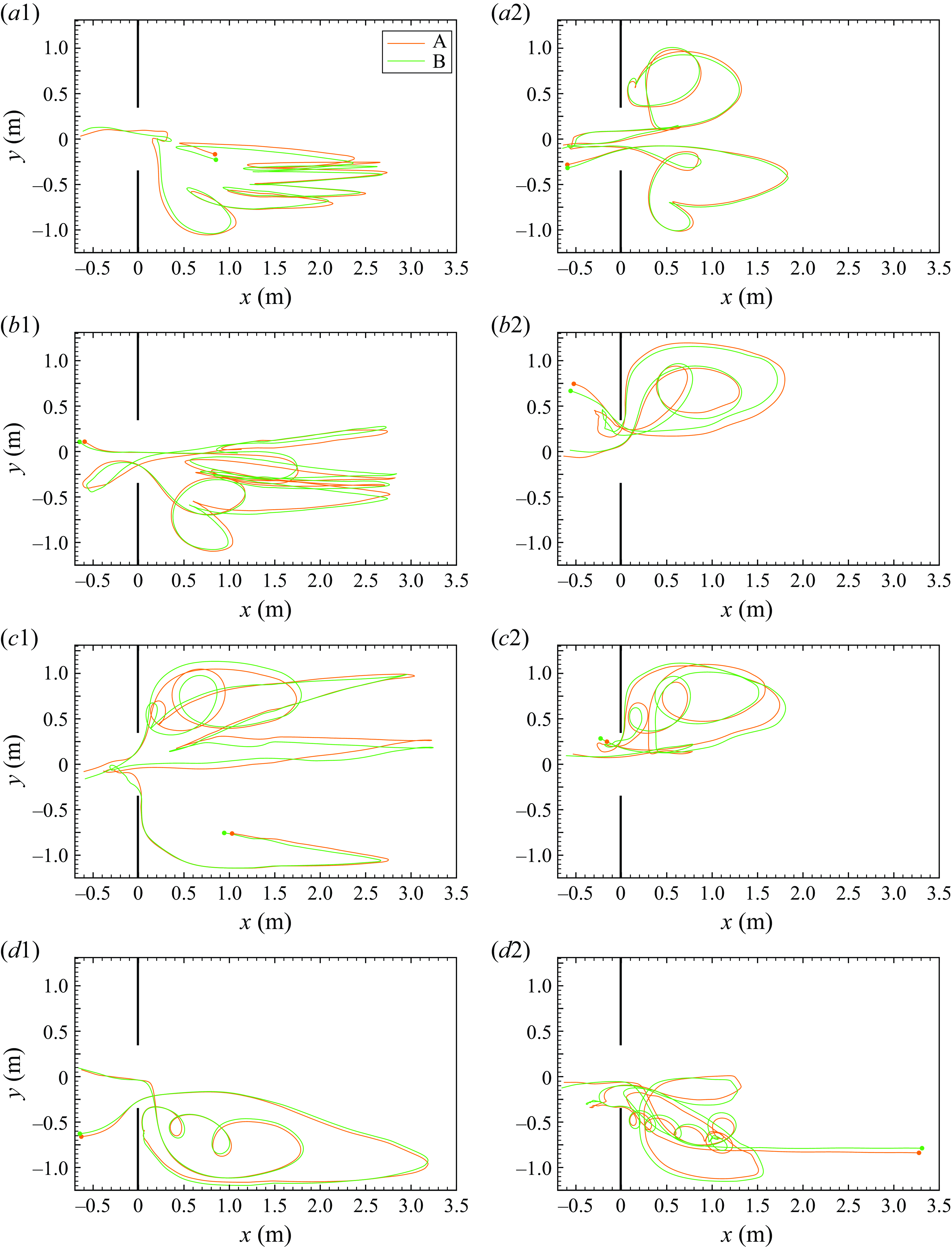
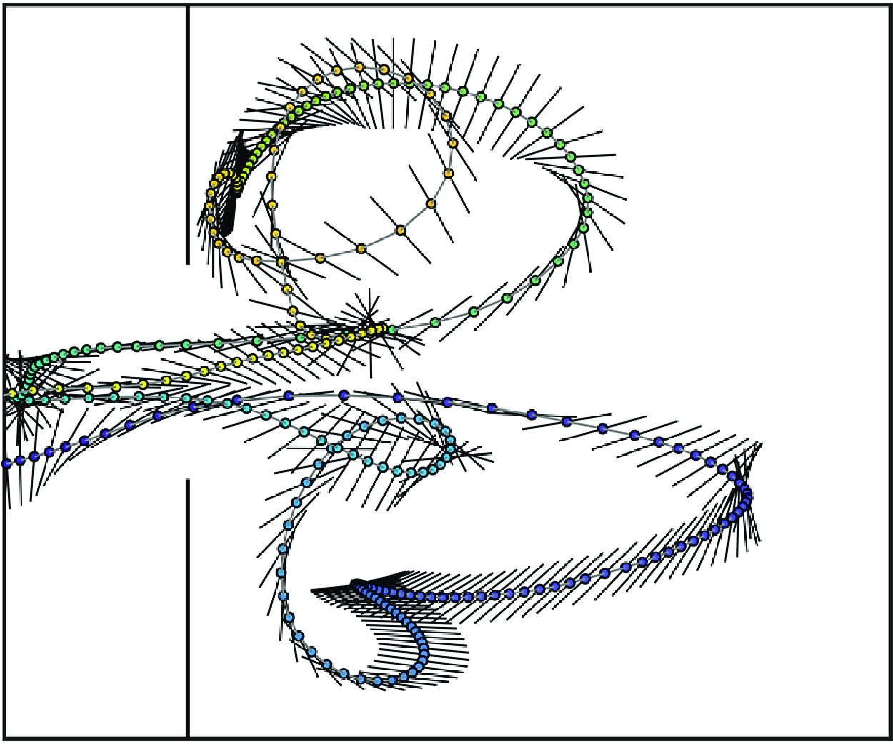
Figure 5. Examples of fibre trajectories observed during the experiments: (a1) experiment 1, fibre of class 02; (a2) experiment 1, fibre of class 01; (b1) experiment 2, fibre of class 02; (b2) experiment 2, fibre of class 03; (c1) experiment 3, fibre of class 03; (c2) experiment 3, fibre of class 03; (d1) experiment 4, fibre of class 01; (d2) experiment 4, fibre of class 02. Here, A and B refer to the fibre ends, and the dots indicate the initial positions of the fibres’ poles.
Figure 4 shows all trajectories of the fibres’ centroids ( $\boldsymbol{X}_C(t)$
) measured during experiments 1, 2, 3 and 4. The three classes of fibres are shown in different colours. By inspecting the four panels, it can be observed that a reasonably good coverage of the entire domain was achieved in the four experiments. The only exceptions are the regions in the lateral corners at the inlet barriers on the basin side, where no fibres are detected. This is consistent with the presence of Lagrangian Coherent Structures, which tend to keep those regions dynamically separated from the most active part of the domain (De Leo et al. Reference De Leo, Enrile and Stocchino2022a
). Moreover, the fibre centroid trajectories clearly mark not only the presence of the two large-scale gyres as a signature of the residual currents shown in figure 3, but also the trace of smaller-scale vortices generated during the flood phase, when the main flow direction is from the open basin towards the tidal channel. It is also possible to detect where the fibres were not engulfed in the large macro-vortices but rather remained in the part of the channel where the flow was smoother and periodically reversed the main direction, approximately for
$\boldsymbol{X}_C(t)$
) measured during experiments 1, 2, 3 and 4. The three classes of fibres are shown in different colours. By inspecting the four panels, it can be observed that a reasonably good coverage of the entire domain was achieved in the four experiments. The only exceptions are the regions in the lateral corners at the inlet barriers on the basin side, where no fibres are detected. This is consistent with the presence of Lagrangian Coherent Structures, which tend to keep those regions dynamically separated from the most active part of the domain (De Leo et al. Reference De Leo, Enrile and Stocchino2022a
). Moreover, the fibre centroid trajectories clearly mark not only the presence of the two large-scale gyres as a signature of the residual currents shown in figure 3, but also the trace of smaller-scale vortices generated during the flood phase, when the main flow direction is from the open basin towards the tidal channel. It is also possible to detect where the fibres were not engulfed in the large macro-vortices but rather remained in the part of the channel where the flow was smoother and periodically reversed the main direction, approximately for $x\gtrsim 2$
m. In fact, fibres released in the farthest part of the tidal channel tended to remain confined outside the main flow structures, and they showed almost rectilinear trajectories that reversed every tidal half-cycle, following the flood and ebb phase cycle. This is again consistent with the Lagrangian Coherent Structures dynamics reported in De Leo et al. (Reference De Leo, Enrile and Stocchino2022a
).
$x\gtrsim 2$
m. In fact, fibres released in the farthest part of the tidal channel tended to remain confined outside the main flow structures, and they showed almost rectilinear trajectories that reversed every tidal half-cycle, following the flood and ebb phase cycle. This is again consistent with the Lagrangian Coherent Structures dynamics reported in De Leo et al. (Reference De Leo, Enrile and Stocchino2022a
).
A better insight into the qualitative behaviour of the fibre trajectories could be inferred by analysing some examples of fibre trajectories, as shown in figure 5. The plots in each row correspond to a single experiment, from experiment 1 to experiment 4. For each experiment, two trajectories are shown as examples: Class 01 in figures 5(a2,d1), class 02 in figures 5(a1,b1,d2), and class 03 in figures 5(b2,c1,c2). The trajectories are displayed as two lines corresponding to the two poles of the fibre: the path of pole A is in orange, and the path of pole B is in green. The initial position of each fibre is marked with a dot of the colour of the corresponding pole. All displayed trajectories lasted for more than a tidal period, thus experiencing all phases of the background flow, namely the accelerating and decelerating flood that controls the generation of vortices in a wide range of scales (up to large gyre occupying the entire channel expansion area) and the accelerating and decelerating ebb when the flow reverses and destroys the large-scale vortices in the channel.
An interesting feature that is easily identified in the fibre trajectories is that they tend to remain confined in the half of the channel where they were initially released or tracked. Very few exceptions to the latter behaviour were observed: two cases are shown in figures 5(a1,c1), for experiments 1 and 3, respectively. In general, the fibres are engulfed inside the lateral macro-vortices, producing looping trajectories, like the cases in experiment 4. Moreover, it is evident that fibres often exhibit tumbling trajectories on scales much smaller than the lateral macro-vortices; see, for example, figures 5(b1,c1,c2,d1,d2). In these cases, the tumbling frequencies are clearly much higher than the tidal period, and it is reasonable to assume that they are driven by the Eulerian flow structure at the scale of the fibre. This aspect will be discussed in detail in the following sections.
3.3. Instantaneous and projected velocity signals
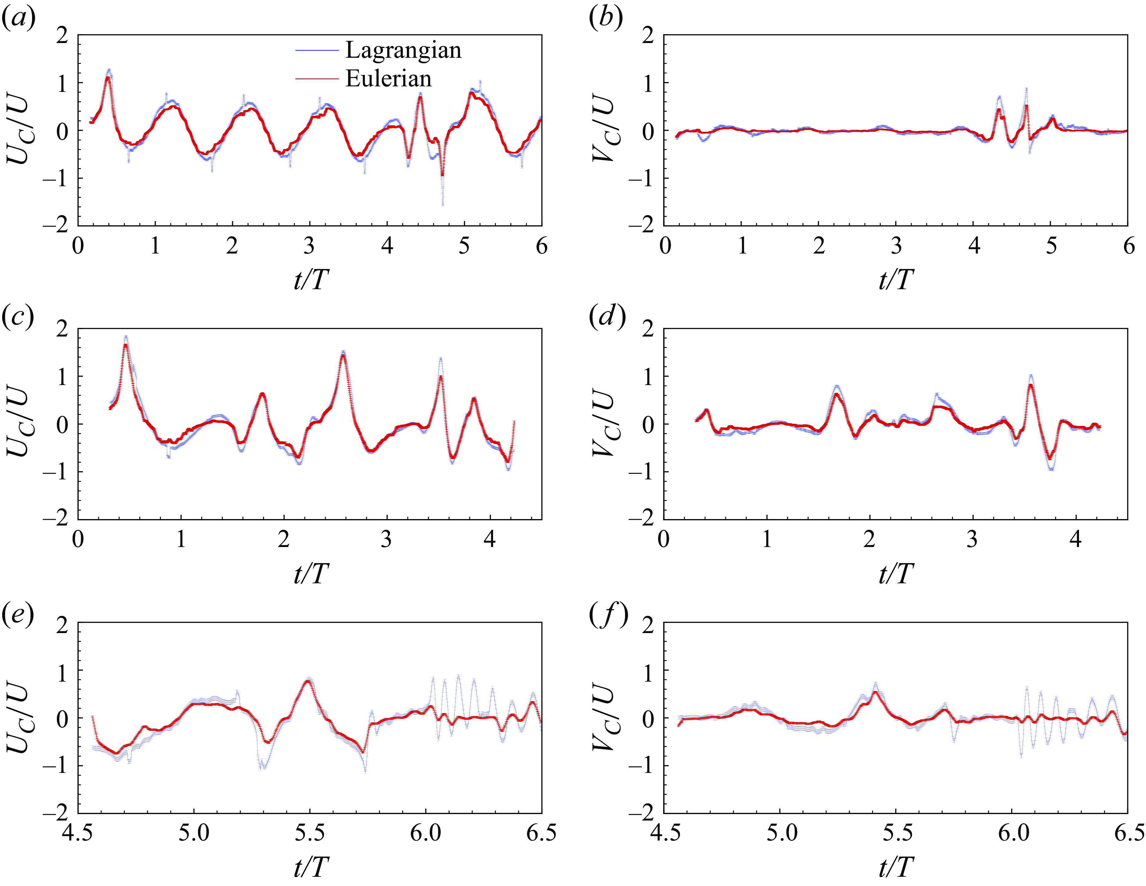
Figure 6. Comparisons between the non-dimensional fibre centroid Lagrangian velocities (blue lines) and the corresponding Eulerian fluid velocities (red lines): (a,c,e) longitudinal velocities of trajectories in figures 5(b1,a2,d2), respectively; (b,d,f) transversal velocities of the same trajectories. The signals are normalised with the velocity $U$
; see table 1.
$U$
; see table 1.
In this section, we compare the instantaneous velocity signals of the fibres’ centroids, resulting from the FTV (Lagrangian) and PIV (Eulerian) measurements, and the projected velocities computed using (2.6) and (2.7). All velocities are made dimensionless using the velocity scale $U$
, reported in table 1.
$U$
, reported in table 1.
Figure 6 shows the comparison between the dimensionless Lagrangian velocity components of the fibres’ centroids ( $\textbf {V}_C=(U_C,V_C)$
) and the corresponding dimensionless Eulerian velocity components interpolated at the centroid location (the fluid flow seen by fibre;
$\textbf {V}_C=(U_C,V_C)$
) and the corresponding dimensionless Eulerian velocity components interpolated at the centroid location (the fluid flow seen by fibre; $\textbf {u}_C=(u_C,v_C)$
).
$\textbf {u}_C=(u_C,v_C)$
).
To help the presentation and the discussion of the velocity signals, we considered only some examples of fibre trajectories shown in figure 5 as prototypes of the possible fibre behaviours. In fact, we can observe that the fibres exhibit different velocity trends depending on their position in space and on the tidal phase. Based on the overall behaviour of the fibres, we tried to group their trajectories into three categories. Note that this was done without following any quantitative criterion, instead considering their time evolution and the Eulerian flow structures that they experienced.
First, we identified fibres whose motion strictly follows the mean periodic flow (controlled by the tidal period), with the longitudinal velocity as the main component. Examples are the trajectories shown in figure 5(a1), whose instantaneous velocity components are shown in figures 6(a,b), and in figure 5(b1). The comparison between panels (a) and (b) suggests that the longitudinal component $U_C/U$
is much higher than the transversal component
$U_C/U$
is much higher than the transversal component $V_C/U$
. Moreover, the periodicity of
$V_C/U$
. Moreover, the periodicity of $U_C/U$
is consistently equal to the tidal period
$U_C/U$
is consistently equal to the tidal period $T$
for most of the trajectory duration, approximately six tidal periods. However, oscillations of
$T$
for most of the trajectory duration, approximately six tidal periods. However, oscillations of $U_C/U$
with a period much shorter than
$U_C/U$
with a period much shorter than $T$
are observed as transient events (time range between
$T$
are observed as transient events (time range between $t/T\sim 4$
and
$t/T\sim 4$
and $t/T\sim 5$
), associated with the interaction of the fibre with Eulerian flow vortices with a typical size of a few fibre lengths
$t/T\sim 5$
), associated with the interaction of the fibre with Eulerian flow vortices with a typical size of a few fibre lengths $L$
. As further proof, the transversal velocity
$L$
. As further proof, the transversal velocity $V_C/U$
shows similar oscillations compared to
$V_C/U$
shows similar oscillations compared to $U_C/U$
in intensity and periodicity, with a phase shift between the velocity components as a signature of fibre tumbling.
$U_C/U$
in intensity and periodicity, with a phase shift between the velocity components as a signature of fibre tumbling.
A second group of fibre trajectories is characterised by instantaneous velocities time signals $U_C/U$
and
$U_C/U$
and $V_C/U$
as the ones reported in figures 6(c,d). In this case, the intensities of the velocity components are closer compared to the previous case. Moreover, the periodicity with
$V_C/U$
as the ones reported in figures 6(c,d). In this case, the intensities of the velocity components are closer compared to the previous case. Moreover, the periodicity with $T$
is less evident, and the signals seem to oscillate over a broader frequency spectrum. This behaviour is ascribed to trajectories of the kind shown in figures 5(a2,b2), where the fibres are transported within the lateral macro-vortices.
$T$
is less evident, and the signals seem to oscillate over a broader frequency spectrum. This behaviour is ascribed to trajectories of the kind shown in figures 5(a2,b2), where the fibres are transported within the lateral macro-vortices.
Whenever the fibres experience flow structures much smaller than the lateral macro-vortices, the instantaneous velocities show a periodic behaviour in both velocity components with a much shorter period than the main tidal forcing. Examples are shown in figures 6(e,f), in particular for $6\lt t/T\lt 6.5$
. The velocities shown in these plots correspond to the trajectory in figure 5(d2), but we obtained similar observations whenever small-scale looping trajectories are identified, e.g. figures 5(c2,d1).
$6\lt t/T\lt 6.5$
. The velocities shown in these plots correspond to the trajectory in figure 5(d2), but we obtained similar observations whenever small-scale looping trajectories are identified, e.g. figures 5(c2,d1).
Finally, a few general aspects can be discussed based on the above results. The time signals of the Lagrangian and fluid seen by fibre velocities (Eulerian) seem to overlap in all cases, but only when short-period events occur. In these cases, the fibre velocities are set in oscillations, with a relatively high amplitude, by the small-scale flow structures, whereas the fluid seen by the fibre signal seems to smooth them out. Another important point is that the behaviours described above are qualitatively valid regardless of the fibre class and the Reynolds number. Differences might arise in terms of velocity intensities while preserving the typical frequencies of oscillations. We will return to this aspect later in the paper.
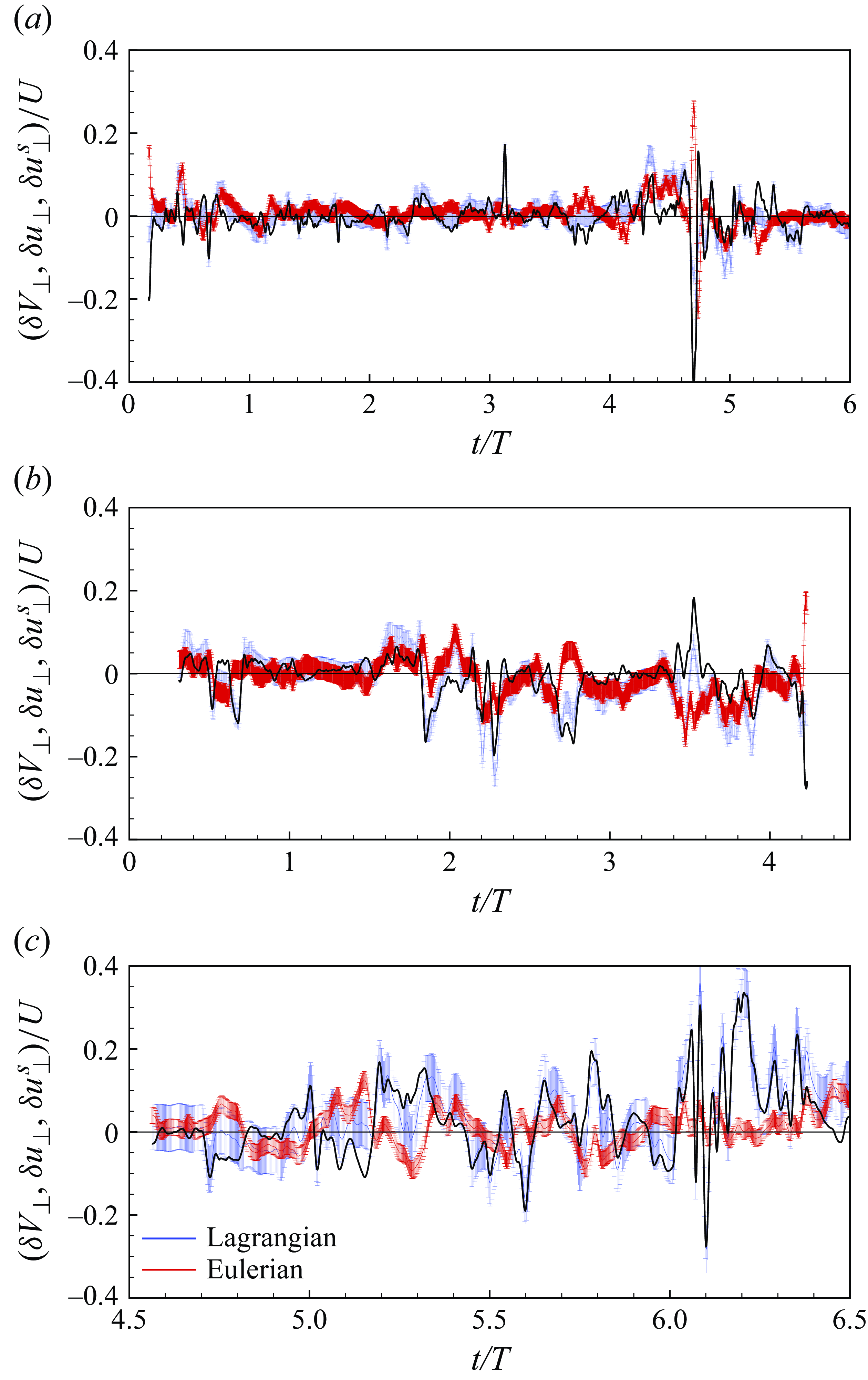
Figure 7. Comparisons between Lagrangian ( $\delta V_{\bot }$
, blue lines) and Eulerian (
$\delta V_{\bot }$
, blue lines) and Eulerian ( $\delta u_{\bot }$
, red lines) transversal projected velocities. The black solid line is the rotational slip velocity (
$\delta u_{\bot }$
, red lines) transversal projected velocities. The black solid line is the rotational slip velocity ( $\delta u^s$
), namely the difference between Lagrangian and Eulerian signals (2.8). The signals are normalised with
$\delta u^s$
), namely the difference between Lagrangian and Eulerian signals (2.8). The signals are normalised with $U$
in table 1. Projected and slip velocity inferred by: (a) instantaneous components of figures 6(a,b); (b) instantaneous components of figures 6(c,d); (c) instantaneous components of figures 6(e,f).
$U$
in table 1. Projected and slip velocity inferred by: (a) instantaneous components of figures 6(a,b); (b) instantaneous components of figures 6(c,d); (c) instantaneous components of figures 6(e,f).
Regarding the projected velocities, figure 7 compares the Lagrangian ( $\delta V_{\bot }$
) and Eulerian (
$\delta V_{\bot }$
) and Eulerian ( $\delta u_{\bot }$
) transverse projected velocities, which are responsible for the fibre’s rotation ((2.6) and (2.7)). These signals are shown along with their confidence levels, calculated starting from the known uncertainties of the measured quantities, namely the displacements. We then propagated the error to all variables derived from the direct measures with the assumption of treating uncorrelated variables and a nonlinear variance propagation (Ku Reference Ku1966; Taylor Reference Taylor1997; Fornasini Reference Fornasini2008). Moreover, the rotational slip velocity (
$\delta u_{\bot }$
) transverse projected velocities, which are responsible for the fibre’s rotation ((2.6) and (2.7)). These signals are shown along with their confidence levels, calculated starting from the known uncertainties of the measured quantities, namely the displacements. We then propagated the error to all variables derived from the direct measures with the assumption of treating uncorrelated variables and a nonlinear variance propagation (Ku Reference Ku1966; Taylor Reference Taylor1997; Fornasini Reference Fornasini2008). Moreover, the rotational slip velocity ( $\delta u_{\bot }^s$
) in (2.8) is also reported as a solid black line.
$\delta u_{\bot }^s$
) in (2.8) is also reported as a solid black line.
Comparing individual trajectories, both Lagrangian and Eulerian signals follow similar overall trends, indicating that the general motion patterns are consistent between the two perspectives. However, figure 7 highlights higher differences, particularly in correspondence of localised peaks, which result in significantly non-zero rotational slip velocities. Furthermore, we can note that the discrepancies between the two signals vary according to the trajectory considered, i.e. the spatial domain explored by each fibre and the phase of the tidal cycle. This means that variations in location and phase, i.e. flow scales experienced by the fibre, can lead to differences in velocity intensities. For example, when the fibres’ trajectories are driven mainly by the large-scale tidal flow (e.g. figure 5
b1), both instantaneous and projected fibre Lagrangian velocities nicely overlap with the Eulerian counterpart; compare figures 6(a,b) and 7(a). On the contrary, the high frequency oscillations detected for example in figures 6(e,f) result in an even larger difference in the projected velocities; see figure 7(c) for $t/T\gt 6$
. Surprisingly, the differences between
$t/T\gt 6$
. Surprisingly, the differences between $\delta V_{\bot }$
and
$\delta V_{\bot }$
and $\delta u_{\bot }$
of figure 7(b) are relatively large in several time intervals, e.g.
$\delta u_{\bot }$
of figure 7(b) are relatively large in several time intervals, e.g. $t/T\sim 2.8$
and
$t/T\sim 2.8$
and $t/T\sim 3.5$
, despite the similarities in the instantaneous signals (same plot of figures 6
c,d). This is apparently in contrast to previous works where projecting the velocities increased the superposition between the Lagrangian and Eulerian velocities along single fibre trajectories (Cavaiola et al. Reference Cavaiola, Olivieri and Mazzino2020), at least at low Stokes numbers. The main reason could be ascribed to the different nature of the underlying Eulerian flow, which is turbulent at moderate Reynolds number in the present case.
$t/T\sim 3.5$
, despite the similarities in the instantaneous signals (same plot of figures 6
c,d). This is apparently in contrast to previous works where projecting the velocities increased the superposition between the Lagrangian and Eulerian velocities along single fibre trajectories (Cavaiola et al. Reference Cavaiola, Olivieri and Mazzino2020), at least at low Stokes numbers. The main reason could be ascribed to the different nature of the underlying Eulerian flow, which is turbulent at moderate Reynolds number in the present case.
Finally, it appears that the instantaneous velocity signals of the centroids (related to translation) are almost indistinguishable between the Eulerian and Lagrangian samplings (figure 6). In contrast, the velocity projections (related to rotation) are generally more dissimilar. In the latter regard, it can be seen that even if the two signals have similar patterns, they may differ significantly instantaneously when the fibre rotation experiences strong fluctuations. This effect can be attributed to the sub-resolution turbulent fluctuations, which are not probed in the Eulerian measurements (see § 3.1), but it can nevertheless contribute to the instantaneous fibre rotation (Shapiro & Goldenberg Reference Shapiro and Goldenberg1993). In this regard, it is worth noting that an infinitely resolved PIV measurement at the fibre location would not change these observations, as it would probe the no-slip condition imposed by the fibre on the flow, resulting in a trivial equivalence between the two signals. In fact, past experiments always relied on a coarse-graining of the velocity gradients field in the fibres’ surroundings for a meaningful comparison (Parsa et al. Reference Parsa, Guasto, Kishore, Ouellette, Gollub and Voth2011; Ni et al. Reference Ni, Kramel, Ouellette and Voth2015; Pujara et al. Reference Pujara, Voth and Variano2019), which is, in our case, provided by the PIV resolution directly. Finally, comparing the coarse-grained flow to the fibre velocity requires to assume that the feedback of the fibre on the flow at scales larger than the fibre length is negligible. This assumption is justified in our experiments by the small mass fraction occupied by the fibres (Olivieri et al. Reference Olivieri, Mazzino and Rosti2022), even compared to the volume of fluid in their surroundings.
3.4. Flow and fibre related statistics
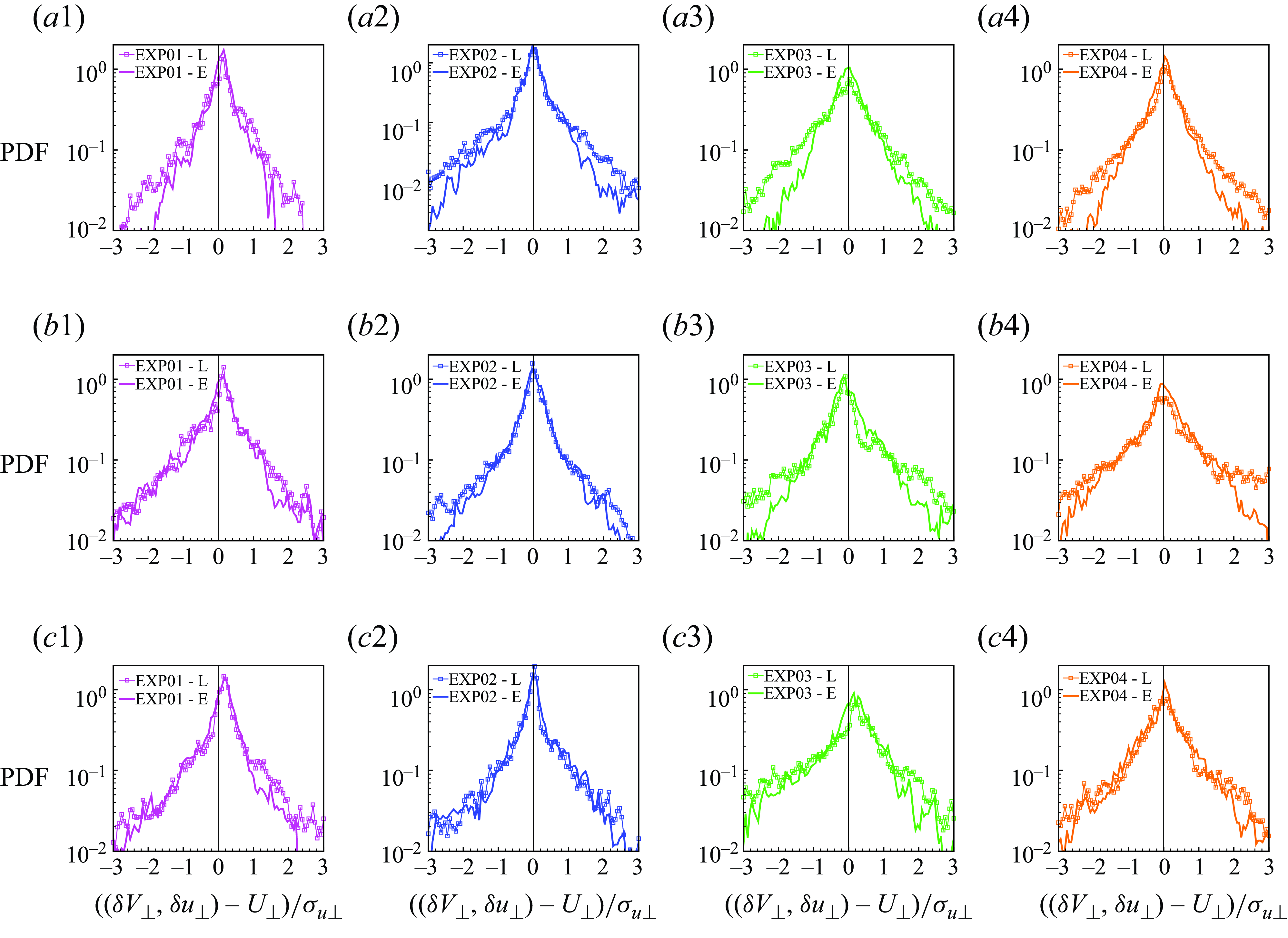
Figure 8. Probability distributions of the projected velocity fluctuations for all experiments and all fibre classes. Rows (a), (b) and (c) correspond to the fibre Class 01 (short), 02 (intermediate) and 03 (long), respectively. The numbers from 1 to 4 (columns) correspond to the experiment labels, from the smallest to the largest Reynolds number.
In the previous section, we presented and discussed the observations considering the single fibre in terms of both trajectories and velocities time series. Herein, we are interested in analysing the fibre dynamics from a statistical point of view, using a few important target quantities, namely the projected velocities and the structure functions. In particular, we aim to compare the Lagrangian (fibre) statistics with the Eulerian (fluid) statistics, and to understand to what extent we could consider the fibre as a proxy for the underlying turbulent Eulerian flow.
Figure 8 shows a comparison between the Lagrangian and Eulerian probability density functions (PDFs) of the normalised projected velocity fluctuations for each fibre class and experiment, i.e.
 \begin{equation} (\delta V_{\bot }-U_{\bot })/\sigma _{U_{\bot }}, \quad (\delta u_{\bot }-U_{\bot })/\sigma _{U_{\bot }}, \end{equation}
where $U_{\bot } = \langle \delta u_{\bot } \rangle$
and
$U_{\bot } = \langle \delta u_{\bot } \rangle$
and $\sigma _{U_{\bot }} = \langle ( \delta u_{\bot } - U_{\bot } )^2 \rangle ^{1/2}$
are the Eulerian mean and standard deviation, respectively, calculated for each fibre class and experiment. Note that both the Lagrangian and Eulerian projected velocity fluctuations have been calculated by subtracting the same mean value (
$\sigma _{U_{\bot }} = \langle ( \delta u_{\bot } - U_{\bot } )^2 \rangle ^{1/2}$
are the Eulerian mean and standard deviation, respectively, calculated for each fibre class and experiment. Note that both the Lagrangian and Eulerian projected velocity fluctuations have been calculated by subtracting the same mean value ( $U_{\bot }$
) and normalising with the same standard deviation (
$U_{\bot }$
) and normalising with the same standard deviation ( $\sigma _{U_{\bot }}$
).
$\sigma _{U_{\bot }}$
).
The Lagrangian and Eulerian PDFs show a fairly good agreement over the whole range of normalised projected velocity fluctuations, suggesting that the two frameworks are statistically equivalent despite their instantaneous differences. As a consequence, this result might suggest that the sub-resolution velocity fluctuations, below the PIV resolution, can influence the instantaneous transverse velocity differences but not their means and standard deviations. The major differences between the Eulerian and Lagrangian distributions are observed for the larger values of the projected velocity fluctuations, corresponding to the extreme events of the distribution, as can be seen, for example, in figures 8(a1,b4,c3).
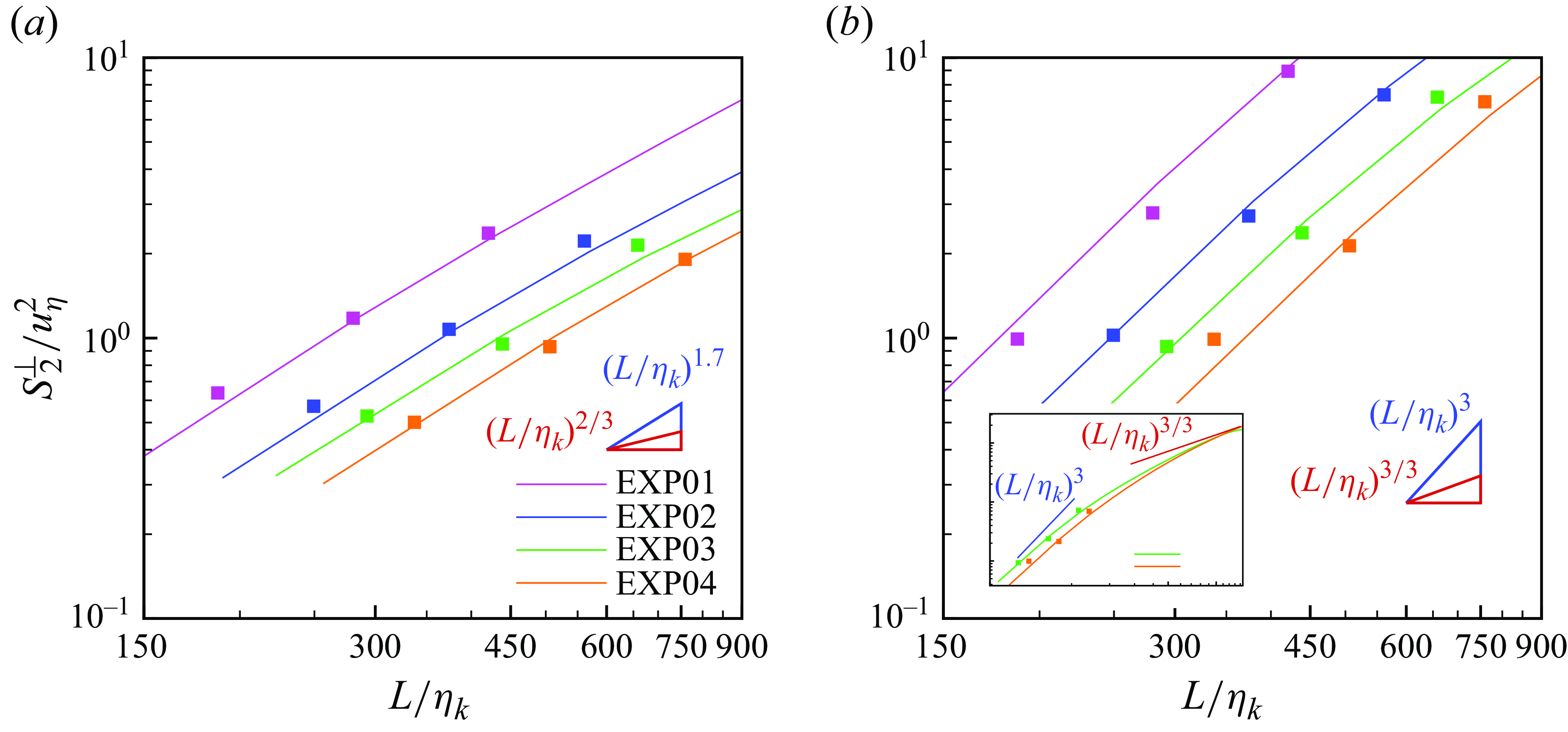
Figure 9. Normalised second- and third-order absolute value structure functions. The solid lines are obtained from the Eulerian signals, whereas the markers are from the fibres’ statistics. (a) Normalised Eulerian (solid lines) and Lagrangian (markers) second-order structure functions. The red triangle represents the K41 power law, while the blue triangle marks the $1.7$
slope. (b) Normalised Eulerian (solid lines) and Lagrangian (markers) third-order absolute structure functions. The red and blue triangles show the linear and cubic power laws, respectively. The inset shows the
$1.7$
slope. (b) Normalised Eulerian (solid lines) and Lagrangian (markers) third-order absolute structure functions. The red and blue triangles show the linear and cubic power laws, respectively. The inset shows the $S_3^{\bot }/u^3_{\eta }$
distribution for experiments 3 and 4 over the full range of scales observed.
$S_3^{\bot }/u^3_{\eta }$
distribution for experiments 3 and 4 over the full range of scales observed.
This observation may be attributed to the effect of the small yet finite fibres inertia, which would, however, lead to weaker tails for more inertial fibres (see the observation of Parsa & Voth (Reference Parsa and Voth2014) in HIT, where longer fibres possess weaker tails). However, in our case, we do not observe any clear trend with fibre length or flow Reynolds number. Furthermore, in some cases – see e.g. the short fibres of Class 01 in figures 8(a1,a2,a3,a4) – the Eulerian PDF tails exceed the fibre one: this can be due to the effect of sub-resolution eddies, which can contribute the fibre rotation but are not captured by the PIV measurement.
We then compared the second- and third-order transverse absolute value structure functions ( $S_2^{\bot }, S_3^{\bot }$
) obtained by the Eulerian (PIV) and Lagrangian (FTV) measurements; see (2.9). The structure functions have been normalised using the Kolmogorov velocity scale, and similarly the fibre length using the Kolmogorov length scale.
$S_2^{\bot }, S_3^{\bot }$
) obtained by the Eulerian (PIV) and Lagrangian (FTV) measurements; see (2.9). The structure functions have been normalised using the Kolmogorov velocity scale, and similarly the fibre length using the Kolmogorov length scale.
Figure 9 shows the normalised structure functions ( $S_2^{\bot }/u^2_{\eta }, S_3^{\bot }/u^3_{\eta }$
) against the normalised fibre length (
$S_2^{\bot }/u^2_{\eta }, S_3^{\bot }/u^3_{\eta }$
) against the normalised fibre length ( $L/\eta _k$
) for all experiments. Solid markers represent the values obtained by averaging the structure functions over the fibres of each class, i.e. we obtained three values for each experiment. The Eulerian
$L/\eta _k$
) for all experiments. Solid markers represent the values obtained by averaging the structure functions over the fibres of each class, i.e. we obtained three values for each experiment. The Eulerian $S_2^{\bot }/u^2_{\eta }$
and
$S_2^{\bot }/u^2_{\eta }$
and $S_3^{\bot }/u^3_{\eta }$
have been computed starting from the PIV fields.
$S_3^{\bot }/u^3_{\eta }$
have been computed starting from the PIV fields.
The results suggest that the FTV-based structure functions can probe the Eulerian structure functions with reasonable accuracy for all four experiments, i.e. for the whole range of Reynolds numbers investigated. In particular, the second-order structure function (figure 9
a), which represents the standard deviation of the transverse velocity fluctuations (see (2.9)), is almost indistinguishable between the two frameworks, whereas the third-order structure function shows slightly higher differences. The latter could be ascribed to the experimental errors, which tend to be amplified with the order of the structure function. However, a more physical explanation could be found in the dynamics of the fibres under more extreme conditions. In fact, as discussed above, also the PDF of the projected velocity fluctuations showed a worse comparison at the extrema of the observed range. It is not surprising that $S_3^{\bot }/u^3_{\eta }$
turns out to be more sensitive to the higher velocity difference, where the fibre showed a longer adaptation time. Nevertheless, the similarity between the structure functions of the Eulerian and fibre-related signals confirms that the eddies of size comparable to the fibre length still drive the fibre rotation, regardless of the specific turbulence structure.
$S_3^{\bot }/u^3_{\eta }$
turns out to be more sensitive to the higher velocity difference, where the fibre showed a longer adaptation time. Nevertheless, the similarity between the structure functions of the Eulerian and fibre-related signals confirms that the eddies of size comparable to the fibre length still drive the fibre rotation, regardless of the specific turbulence structure.
It is now interesting to discuss the scaling of the observed $S_2^{\bot }/u^2_{\eta }$
and
$S_2^{\bot }/u^2_{\eta }$
and $S_3^{\bot }/u^3_{\eta }$
. It is well accepted that in case of HIT, power-law structure functions of the form
$S_3^{\bot }/u^3_{\eta }$
. It is well accepted that in case of HIT, power-law structure functions of the form $S_n \sim ( L/\eta _{k} )^{n/3}$
are expected to hold (Frisch & Kolmogorov Reference Frisch and Kolmogorov1995; Pope Reference Pope2000). This power law behaviour was originally predicted by the K41 theory (Kolmogorov Reference Kolmogorov1941b
), assuming a constant energy flux across inertial range scales.
$S_n \sim ( L/\eta _{k} )^{n/3}$
are expected to hold (Frisch & Kolmogorov Reference Frisch and Kolmogorov1995; Pope Reference Pope2000). This power law behaviour was originally predicted by the K41 theory (Kolmogorov Reference Kolmogorov1941b
), assuming a constant energy flux across inertial range scales.
However, De Leo & Stocchino (2022, Reference De Leo and Stocchino2023) pointed out that in the flow under consideration, the energy cascade exhibits a direct or an inverse behaviour, depending on the phase of the tide. Indeed, the Eulerian structure functions and the corresponding Lagrangian values show a strongly non-K41 behaviour (see the comparison with the $2/3$
and
$2/3$
and $3/3$
slopes, in red in figures 9
a,b) with an
$3/3$
slopes, in red in figures 9
a,b) with an $S_2$
exponent closer to
$S_2$
exponent closer to $1.7$
, a value often observed in two-dimensional turbulence (Belmonte et al. Reference Belmonte, Goldburg, Kellay, Rutgers, Martin and Wu1999; Goldburg et al. Reference Goldburg, Cressman, Vörös, Eckhardt and Schumacher2001; Rivera et al. Reference Rivera, Daniel, Chen and Ecke2003; Paraz & Bandi Reference Paraz and Bandi2019). Note that the range of scales covered by the three fibre classes is
$1.7$
, a value often observed in two-dimensional turbulence (Belmonte et al. Reference Belmonte, Goldburg, Kellay, Rutgers, Martin and Wu1999; Goldburg et al. Reference Goldburg, Cressman, Vörös, Eckhardt and Schumacher2001; Rivera et al. Reference Rivera, Daniel, Chen and Ecke2003; Paraz & Bandi Reference Paraz and Bandi2019). Note that the range of scales covered by the three fibre classes is $190\lesssim L/\eta _{k}\lesssim 800$
, i.e. within the inertial range.
$190\lesssim L/\eta _{k}\lesssim 800$
, i.e. within the inertial range.
However, the peculiar scaling of both $S_2$
and
$S_2$
and $S_3$
can result from a combination of causes, such as the free surface compressibility (Rivera et al. Reference Rivera, Vorobieff and Ecke1998), the presence of a sustained external force (Boffetta & Musacchio Reference Boffetta and Musacchio2010), the non-homogeneity of the domain, i.e. water depth variability acting as a geometric constraint on the turbulent flow (Stocchino & Brocchini Reference Stocchino and Brocchini2010; Stocchino et al. Reference Stocchino, Besio, Angiolani and Brocchini2011), and in general, the strongly non-idealised flow conditions. The typical signature of an inverse energy cascade is the change of sign of the nonlinear energy fluxes at the injection scale (Boffetta & Musacchio Reference Boffetta and Musacchio2010; Alexakis & Biferale Reference Alexakis and Biferale2018). In the present context of periodical turbulent flow, the injection scale was found to be proportional to the length of the tidal barrier (
$S_3$
can result from a combination of causes, such as the free surface compressibility (Rivera et al. Reference Rivera, Vorobieff and Ecke1998), the presence of a sustained external force (Boffetta & Musacchio Reference Boffetta and Musacchio2010), the non-homogeneity of the domain, i.e. water depth variability acting as a geometric constraint on the turbulent flow (Stocchino & Brocchini Reference Stocchino and Brocchini2010; Stocchino et al. Reference Stocchino, Besio, Angiolani and Brocchini2011), and in general, the strongly non-idealised flow conditions. The typical signature of an inverse energy cascade is the change of sign of the nonlinear energy fluxes at the injection scale (Boffetta & Musacchio Reference Boffetta and Musacchio2010; Alexakis & Biferale Reference Alexakis and Biferale2018). In the present context of periodical turbulent flow, the injection scale was found to be proportional to the length of the tidal barrier ( $l_w$
). Moreover, De Leo & Stocchino (2022) showed that the dominant energy process, after averaging in space and time (over the tidal period), was indeed an inverse energy cascade. The two-dimensional inverse energy process studied in configuration space, i.e. using the velocity increments, yields a specific scaling for the longitudinal and transversal structure functions, namely
$l_w$
). Moreover, De Leo & Stocchino (2022) showed that the dominant energy process, after averaging in space and time (over the tidal period), was indeed an inverse energy cascade. The two-dimensional inverse energy process studied in configuration space, i.e. using the velocity increments, yields a specific scaling for the longitudinal and transversal structure functions, namely $S_3(l) \varpropto l^3$
for scales smaller than the injection scale, and
$S_3(l) \varpropto l^3$
for scales smaller than the injection scale, and $S_3(l) \varpropto l$
for scales larger than the injection scale, where
$S_3(l) \varpropto l$
for scales larger than the injection scale, where $l$
is the increment (Boffetta & Musacchio Reference Boffetta and Musacchio2010; Alexakis & Biferale Reference Alexakis and Biferale2018). Figure 9(b) shows the distribution of
$l$
is the increment (Boffetta & Musacchio Reference Boffetta and Musacchio2010; Alexakis & Biferale Reference Alexakis and Biferale2018). Figure 9(b) shows the distribution of $S_3^{\bot }/u^3_{\eta }$
together with the theoretical power laws (blue and red triangles) in the range covered by the fibre length (main plot) and for a wider range in the inset. In the latter, only two experiments (3 and 4) are shown for clarity. In a previous study of the tidal flow under investigation, the injection scale was estimated to be proportional to the inlet barrier length
$S_3^{\bot }/u^3_{\eta }$
together with the theoretical power laws (blue and red triangles) in the range covered by the fibre length (main plot) and for a wider range in the inset. In the latter, only two experiments (3 and 4) are shown for clarity. In a previous study of the tidal flow under investigation, the injection scale was estimated to be proportional to the inlet barrier length $l_w$
, and specifically
$l_w$
, and specifically $l_{inj}\sim 0.2 l_w$
, which corresponds to
$l_{inj}\sim 0.2 l_w$
, which corresponds to $l_{inj}/\eta _k \approx 1000{-}2000$
using the Kolmogorov length scale for normalisation. Thus theoretically, we expect a change in slope at
$l_{inj}/\eta _k \approx 1000{-}2000$
using the Kolmogorov length scale for normalisation. Thus theoretically, we expect a change in slope at $l/\eta _{k}\approx l_{inj}/\eta _k$
. The distribution of
$l/\eta _{k}\approx l_{inj}/\eta _k$
. The distribution of $S_3^{\bot }/u^3_{\eta }$
in our experiment shows a two-slope behaviour, with a steeper value for
$S_3^{\bot }/u^3_{\eta }$
in our experiment shows a two-slope behaviour, with a steeper value for $l/\eta _{k}\lt l_{inj}/\eta _k$
, and tending towards linearity for
$l/\eta _{k}\lt l_{inj}/\eta _k$
, and tending towards linearity for $l/\eta _{k}\gt l_{inj}/\eta _k$
. In the first range, which corresponds to a direct energy cascade, we estimate exponent 2.5, which is slightly lower than the theoretical value 3, as shown in the case of forced turbulence discussed in Boffetta & Musacchio (Reference Boffetta and Musacchio2010), in particular, for their numerical experiment with the highest Reynolds number. This discrepancy might be ascribed to two main reasons. First, the Reynolds number of the present experiment attains only moderate values, and it might affect the power laws expected for infinite Reynolds number (Antonia et al. Reference Antonia, Satyaprakash and Chambers1982; Boffetta & Romano Reference Boffetta and Romano2002; Antonia et al. Reference Antonia, Tang, Djenidi and Zhou2019). Second, we used the absolute or relative third-order structure function, whose slopes might be slightly different from the standard definition (Arneodo et al. Reference Arneodo1996). However, the second-order structure function is expected to be quadratic in association with a direct energy cascade, and indeed, our experiment shows a value close to the theoretical one (Casciola et al. Reference Casciola, Benzi, Gualtieri, Jacob and Piva2001; Kellay & Goldburg Reference Kellay and Goldburg2002; Boffetta & Ecke Reference Boffetta and Ecke2012), thus reinforcing the conclusions on the existence of an inverse energy process presented in De Leo & Stocchino (2022, Reference De Leo and Stocchino2023).
$l/\eta _{k}\gt l_{inj}/\eta _k$
. In the first range, which corresponds to a direct energy cascade, we estimate exponent 2.5, which is slightly lower than the theoretical value 3, as shown in the case of forced turbulence discussed in Boffetta & Musacchio (Reference Boffetta and Musacchio2010), in particular, for their numerical experiment with the highest Reynolds number. This discrepancy might be ascribed to two main reasons. First, the Reynolds number of the present experiment attains only moderate values, and it might affect the power laws expected for infinite Reynolds number (Antonia et al. Reference Antonia, Satyaprakash and Chambers1982; Boffetta & Romano Reference Boffetta and Romano2002; Antonia et al. Reference Antonia, Tang, Djenidi and Zhou2019). Second, we used the absolute or relative third-order structure function, whose slopes might be slightly different from the standard definition (Arneodo et al. Reference Arneodo1996). However, the second-order structure function is expected to be quadratic in association with a direct energy cascade, and indeed, our experiment shows a value close to the theoretical one (Casciola et al. Reference Casciola, Benzi, Gualtieri, Jacob and Piva2001; Kellay & Goldburg Reference Kellay and Goldburg2002; Boffetta & Ecke Reference Boffetta and Ecke2012), thus reinforcing the conclusions on the existence of an inverse energy process presented in De Leo & Stocchino (2022, Reference De Leo and Stocchino2023).
3.5. Signatures of the turbulence non-ideality on the fibre dynamics
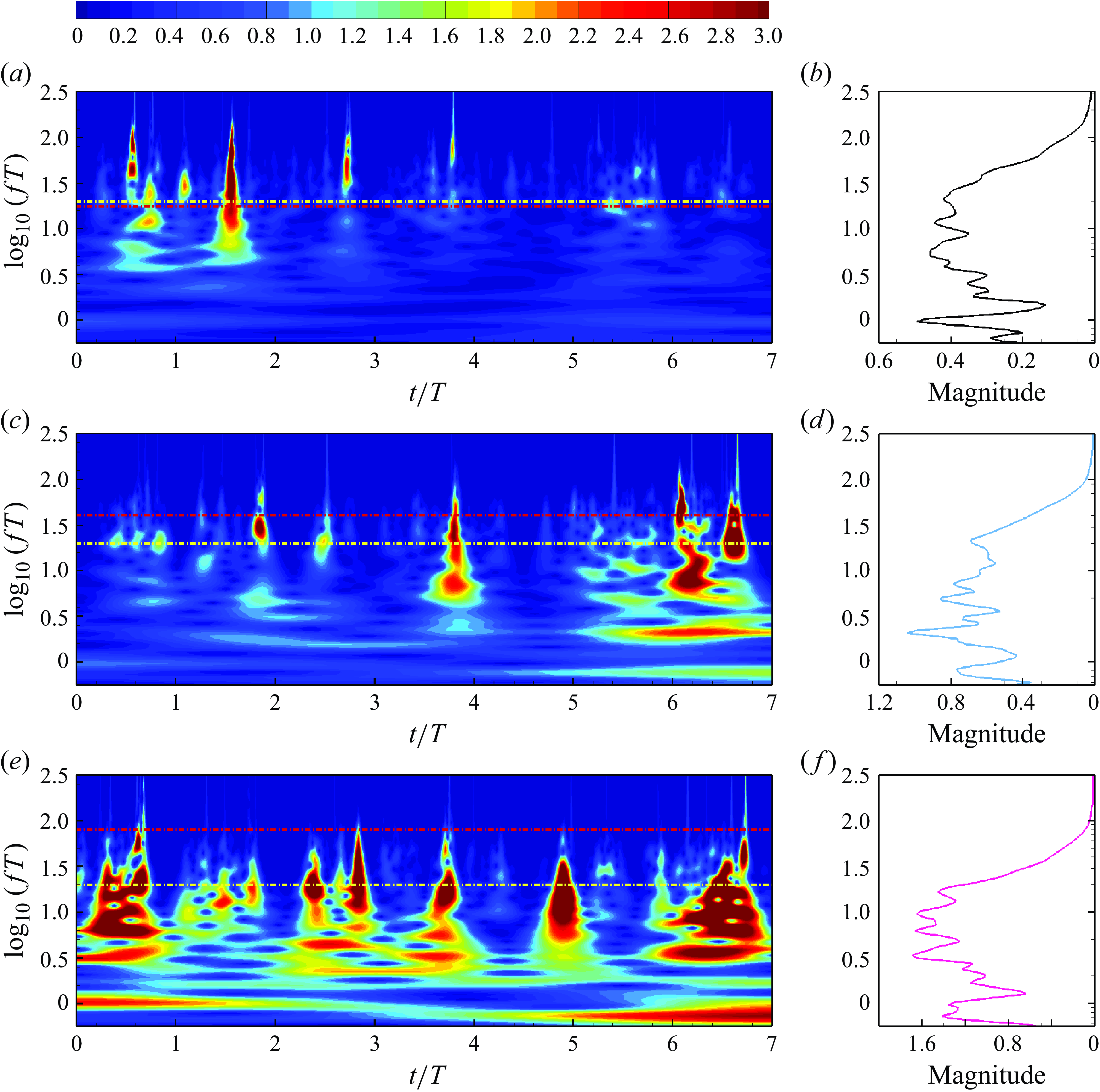
Figure 10. (a,c,e) Wavelet maps of the averaged second-order structure functions, along with (b,d,f) their time averages, corresponding to the Fourier spectra. The plots are obtained from experiment 4 (the largest Reynolds number): (a,b) fibre class 01 (short), (c,d) class 02 (intermediate), and (e,f) class 03 (long). The red dash-dotted line corresponds to the normalised fibre tumbling frequency ( $T/\tau _p$
), and the yellow dash-dotted line to the mean normalised Eulerian vortex turnover frequency (
$T/\tau _p$
), and the yellow dash-dotted line to the mean normalised Eulerian vortex turnover frequency ( $T/T_T$
).
$T/T_T$
).
The section analyses the effect of non-ideal turbulence on the fibre dynamics, focusing mainly on the periodicity and non-stationarity of the flow. The time-averaged statistical analysis presented in § 3.4 cannot fully capture the complex interplay between the fibre motion and the turbulent Eulerian flow. Indeed, at every cycle, a transient energy cascade is produced (De Leo & Stocchino 2022), which may interact with the fibres in different ways depending on the tidal phase. During the early flood phase, a jet of water enters the basin, and the wall inlet sheds small eddies that merge in two separated large-scale stable macro-vortices that could, in principle, rotate the fibres. However, the typical size of these large eddies, approximately equal to the integral length scale of the flow, is much larger than the fibre length, which falls into the inertial range. Thus the fibres are mainly advected and not significantly rotated by these eddies. During the ebb phase, the large eddies fragment and periodically produce an extended turbulent cascade that contains eddies comparable in size with the fibre length. Quantitatively, this process can be described by the wavelet maps of the fibre transverse velocity increments averaged over the fibre ensemble at each time. Indeed, while a simple Fourier analysis does not reveal the interplay between the fibre dynamics and the transient energy cascade, this is visible when considering wavelets, which are complete time-frequency transforms, thus better at examining localised-in-time features in the fibre rotational dynamics (Aswathy & Rosti Reference Aswathy and Rosti2024).
Figure 10 summarises the results of the wavelet analysis for the three classes of fibre during experiment 4 (highest Reynolds number). Figures 10(a,c,e) show the wavelet transform scalogram corresponding to Classes 01, 02 and 03, respectively. The frequency normalised to the tidal period $T$
is reported as
$T$
is reported as $\log_{10}(fT)$
as a function of the non-dimensional time
$\log_{10}(fT)$
as a function of the non-dimensional time $t/T$
. With this choice, the dominant non-dimensional tidal frequency (
$t/T$
. With this choice, the dominant non-dimensional tidal frequency ( $1/T$
) corresponds to the value 0. In the same plots, two other important frequencies are reported as dash-dotted lines. The red line indicates the normalised fibre tumbling frequency (
$1/T$
) corresponds to the value 0. In the same plots, two other important frequencies are reported as dash-dotted lines. The red line indicates the normalised fibre tumbling frequency ( $T/\tau _p$
), and the yellow line indicates the mean normalised Eulerian vortex turnover frequency (
$T/\tau _p$
), and the yellow line indicates the mean normalised Eulerian vortex turnover frequency ( $T/T_T$
). The turnover time
$T/T_T$
). The turnover time $T_T$
is defined as
$T_T$
is defined as $T_T=1/\sqrt {2Z^2}$
, where
$T_T=1/\sqrt {2Z^2}$
, where $Z^2$
is the total enstrophy (calculated as the ensemble averaged square vorticity
$Z^2$
is the total enstrophy (calculated as the ensemble averaged square vorticity $\omega$
,
$\omega$
, $Z^2=\langle\| \boldsymbol{\omega }\|^2/2\rangle$
).
$Z^2=\langle\| \boldsymbol{\omega }\|^2/2\rangle$
).
The wavelet maps in figures 10(a,c,e) show that a particular range of normalised frequencies between $0.5$
and
$0.5$
and $2$
– which is approximately the mean turnover frequency of the turbulent eddies at the fibre’s scale – turns on intermittently at every tidal cycle. This is not the case when considering the Eulerian turnover time signal (figure 11
a), where the tidal frequency (
$2$
– which is approximately the mean turnover frequency of the turbulent eddies at the fibre’s scale – turns on intermittently at every tidal cycle. This is not the case when considering the Eulerian turnover time signal (figure 11
a), where the tidal frequency ( $10^{-2}$
Hz), zero on the vertical axis of the figure, dominates the wavelet map for all times. The contribution of the fibres’ frequencies becomes dominant when they interact with eddies of size comparable with fibre length. Notably, the tidal frequency becomes more present in the wavelet maps for increasing fibre lengths (from figure 10(a) to figure 10(e)), as longer fibres can interact even with the integral scale eddies. Furthermore, the wavelet maps show that the fibre frequencies are activated in a non-perfectly periodic manner. The main reason for the latter behaviour can be attributed to the fact that the fibres are non-homogeneously distributed in space, and this, in addition to the spatial non-homogeneity of the background turbulence, makes them explore regions of different turbulent intensities and structures in each cycle.
$10^{-2}$
Hz), zero on the vertical axis of the figure, dominates the wavelet map for all times. The contribution of the fibres’ frequencies becomes dominant when they interact with eddies of size comparable with fibre length. Notably, the tidal frequency becomes more present in the wavelet maps for increasing fibre lengths (from figure 10(a) to figure 10(e)), as longer fibres can interact even with the integral scale eddies. Furthermore, the wavelet maps show that the fibre frequencies are activated in a non-perfectly periodic manner. The main reason for the latter behaviour can be attributed to the fact that the fibres are non-homogeneously distributed in space, and this, in addition to the spatial non-homogeneity of the background turbulence, makes them explore regions of different turbulent intensities and structures in each cycle.
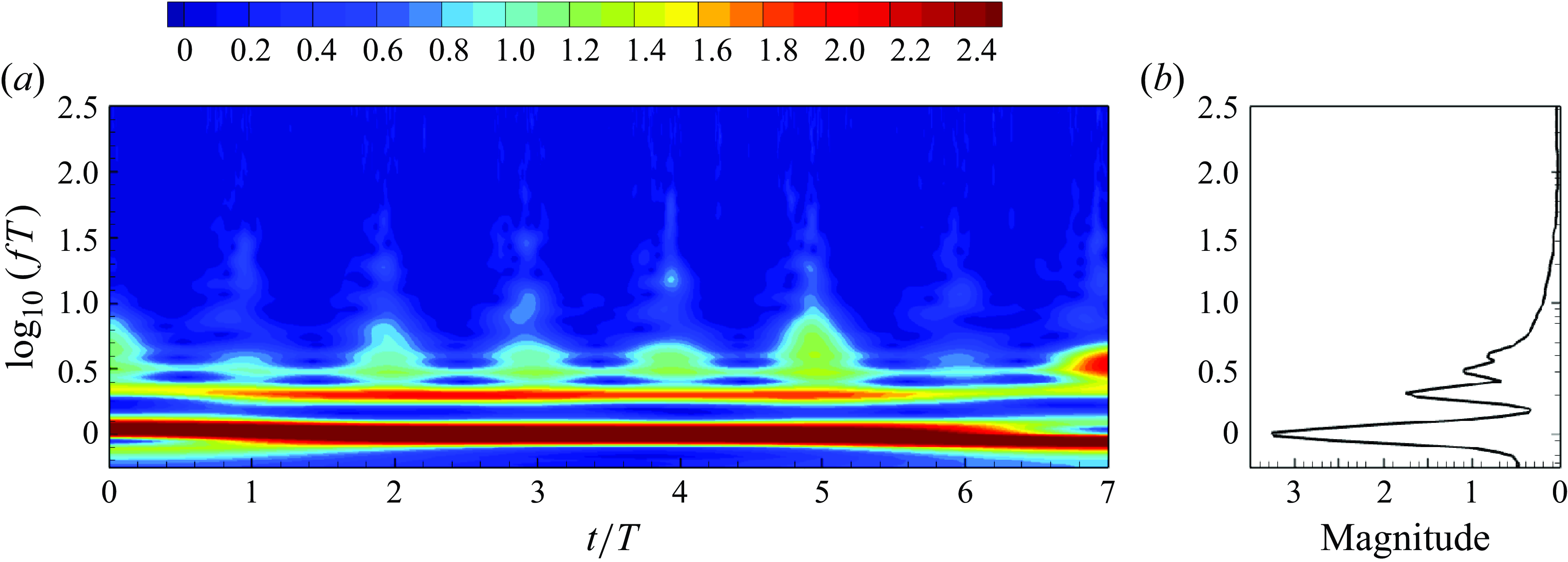
Figure 11. (a) Wavelet map of the Eulerian turnover time, along with (b) its time average, corresponding to the Fourier spectrum. The figure is obtained from experiment 4 (the largest Reynolds number).
Figures 10(b,d,f) show the time-averaged wavelet maps, i.e. the Fourier spectra. These reveal a multi-peaked response of the fibre to the turbulence cascade within the inertial range frequencies, which is absent in the Eulerian signal (figure 11 b).
4. Concluding remarks
We performed large-scale laboratory experiments to study the dynamics of long (whose length falls into the inertial range of turbulence) fibres in a non-homogeneous, non-stationary and non-isotropic free surface turbulence generated by a tidal flow interacting with a tidal inlet. By combining surface PIV with fibre tracking, we studied the interplay between fibre motion and flow, sampled at spatial resolution approximately the fibre length.
Our work reveals that the coupling between the fibre rotational dynamics and the flow is evident when considering statistical observables. At the same time, the instantaneous signals differ significantly between the PIV and fibre-based sampling. This fact has not been observed for short fibres in two-dimensional chaotic flows, where a match between the fibres’ rotational velocity and the prediction provided by the Jeffery model was observed experimentally (Parsa et al. Reference Parsa, Guasto, Kishore, Ouellette, Gollub and Voth2011). This is also the case for Kolmogorov-sized fibres in three-dimensional HIT (Ni et al. Reference Ni, Kramel, Ouellette and Voth2015). However, while all these studies encompass short fibres, which are expected to obey Jeffery’s model, our fibres are long (estimated to be between $200$
and
$200$
and $800$
Kolmogorov scales), and the equivalence between the instantaneous Lagrangian and Eulerian signals is no longer ensured.
$800$
Kolmogorov scales), and the equivalence between the instantaneous Lagrangian and Eulerian signals is no longer ensured.
Nevertheless, the transverse velocity differences statistics are well captured by the fibres in terms of PDFs and structure functions. This means that the scale selection hypothesis, according to which the fibre rotates primarily due to the eddies of its own size (Parsa & Voth Reference Parsa and Voth2014; Bounoua et al. Reference Bounoua, Bouchet and Verhille2018; Pujara et al. Reference Pujara, Voth and Variano2019; Brizzolara et al. Reference Brizzolara, Rosti, Olivieri, Brandt, Holzner and Mazzino2021), generalises to non-idealised conditions. This can be due either to the universality of small-scale motion, meaning that the structure functions become more HIT-like at small scale, or to the fact that the requirements for the scale selection to occur are more general than having ideal turbulence (e.g. having on average a direct energy cascade).
In conjunction with the third-order structure function, the PDFs show that extreme events are harder to capture for long fibres. These fibres are well within the inertial range. The longer the fibre, the less it samples the small-scale velocity fluctuations, where most extreme events concentrate. However, the fibres should be able to capture inertial range intermittency, as they are expected to act as (anisotropic) low-pass filters. This observation may be explained by considering that the small yet finite rotational and translational inertia could alter the fibres’ sensitivity to extreme events. Indeed, one way to quantify the rotational inertia of long fibres in turbulence is by using the Stokes number provided by Bounoua et al. (Reference Bounoua, Bouchet and Verhille2018) ( ${St}^{(b)}$
), which considers the fibres to be within the inertial range of turbulence. However, to derive their Stokes number, the Authors assume that the turbulence is K41-like and delta-correlated in time, which is not true in our experiments because (i) the structure functions are non-K41 (see figure 9), and (ii) the temporal correlation is strongly non-delta (De Leo et al. Reference De Leo, Ruffini, Postacchini, Colombini and Stocchino2020, 2021; De Leo & Stocchino Reference De Leo and Stocchino2023).
${St}^{(b)}$
), which considers the fibres to be within the inertial range of turbulence. However, to derive their Stokes number, the Authors assume that the turbulence is K41-like and delta-correlated in time, which is not true in our experiments because (i) the structure functions are non-K41 (see figure 9), and (ii) the temporal correlation is strongly non-delta (De Leo et al. Reference De Leo, Ruffini, Postacchini, Colombini and Stocchino2020, 2021; De Leo & Stocchino Reference De Leo and Stocchino2023).
As the turbulence is non-homogeneous and non-stationary, the question of how its non-ideality is reflected in the fibre dynamics arises spontaneously. In this regard, the standard statistical approach to analyse the fibre’s rotational statistics by looking at the PDFs and the structure functions is overly simplistic. We therefore employed a wavelet transform, which allowed us to investigate how the fibres coupled with the transient energy cascade generated by the tidal flow. In this context, we found a scenario in which the fibre rotates intermittently only when the turbulence cascade propagates down to the scale of the fibre length. This fact strengthens the generally accepted belief that fibres rotate mainly due to the eddies of their size, namely the scale selection.
From another point of view, our work could be applied to the transport and rotation of mesoscale and macroscale floating litter in the coastal zone (Crawford & Quinn Reference Crawford and Quinn2017; Núñez et al. Reference Núñez, Romano, García-Alba, Besio and Medina2023). Here, the relevant literature mainly focuses on micro-litters (fragments whose size is smaller than $5$
mm), since most fragments – in number – accumulate at microscales due to plastic inertia and self-similar fragmentation (see e.g. Cózar et al. Reference Cózar2014). However, considering mass or volume, the largest contribution to the global balance is provided by meso- and macro-sized litters, with the highest frequency at approximately
$5$
mm), since most fragments – in number – accumulate at microscales due to plastic inertia and self-similar fragmentation (see e.g. Cózar et al. Reference Cózar2014). However, considering mass or volume, the largest contribution to the global balance is provided by meso- and macro-sized litters, with the highest frequency at approximately $30$
cm (see the probability distributions provided by Kaandorp et al. Reference Kaandorp, Lobelle, Kehl, Dijkstra and van Sebille2023). This class of litter falls into the inertial range of oceanic turbulence, where the Kolmogorov scale ranges between
$30$
cm (see the probability distributions provided by Kaandorp et al. Reference Kaandorp, Lobelle, Kehl, Dijkstra and van Sebille2023). This class of litter falls into the inertial range of oceanic turbulence, where the Kolmogorov scale ranges between $0.1$
and
$0.1$
and $10$
mm depending on the sea state and the water depth (Gargett Reference Gargett1989; D’Asaro Reference D’Asaro2014). Attempts to develop a framework for analysing inertial particle motion in the surface ocean using a vertically averaged Maxey–Riley set on spherical objects confirm our findings that the inertial particle velocity exponentially approaches a weighted average of seawater and air velocities, highlighting the role of anticyclonic mesoscale eddies in trapping marine debris (Beron-Vera et al. Reference Beron-Vera, Olascoaga and Miron2019). More complex shapes, such as ellipsoidal particles, have been studied in wave current flows through a parametric study of the Maxey–Riley and Euler equations, considering negatively buoyant dispersion and finding that the settling wave time scale ratio significantly affects particle dispersion (Sunberg et al. Reference Sunberg, DiBenedetto, Ouellette and Koseff2024).
$10$
mm depending on the sea state and the water depth (Gargett Reference Gargett1989; D’Asaro Reference D’Asaro2014). Attempts to develop a framework for analysing inertial particle motion in the surface ocean using a vertically averaged Maxey–Riley set on spherical objects confirm our findings that the inertial particle velocity exponentially approaches a weighted average of seawater and air velocities, highlighting the role of anticyclonic mesoscale eddies in trapping marine debris (Beron-Vera et al. Reference Beron-Vera, Olascoaga and Miron2019). More complex shapes, such as ellipsoidal particles, have been studied in wave current flows through a parametric study of the Maxey–Riley and Euler equations, considering negatively buoyant dispersion and finding that the settling wave time scale ratio significantly affects particle dispersion (Sunberg et al. Reference Sunberg, DiBenedetto, Ouellette and Koseff2024).
In this context, our work contributes to the understanding of the interaction between large litters and ocean turbulence in the coastal zone, specifically focusing on both transport and stress. In particular, the first aspect involves the distribution of fragments in space and time due to the complex flow generated by the tide, whereas the latter offers a first insight into the gradients that act on the particles. We discovered that despite the Lagrangian and Eulerian frameworks being quite similar from a purely statistical point of view, the strong temporal and spatial inhomogeneity of the flow leads the fibres to experience strongly intermittent gradients, which alternate periods of almost zero gradients with strong, localised-in-time, peaks that are more likely to break up the fragments (see time series in figure 7). Our study thus highlights the need to take into account the strong flow non-ideality when forecasting the fate and transport of mesoscale litter.
Acknowledgements.
We would like to thank Professor A. Mazzino for his initial idea on the fibre experiments. We are also deeply thankful to Dr S. Olivieri for his insightful discussions and for suggesting relevant papers.
Funding.
A.S. expresses thanks for support from the Research Grants Council of Hong Kong (project IDs 15216422 and C5032-22EF) and from the Research Institute for Land and Space (RILS) (project ID P0049622). S.B. is funded by the European Union’s Horizon 2020 research and innovation programme under the Marie Skłodowska-Curie grant agreement (no.101034413).
Declaration of interests.
The authors report no conflict of interest.
Author contributions.
A.D.L.: conceptualisation, formal analysis, investigation, resources, data curation, writing – original draft, writing – review and editing, visualisation. S.B.: conceptualisation, formal analysis, writing – original draft, writing – review and editing, funding acquisition. M.C.: conceptualisation, writing – review and editing. J.H.: methodology, data curation, writing – review and editing. A.S.: conceptualisation, investigation, resources, data curation, writing – original draft, writing – review and editing, supervision, funding acquisition.
Data availability statement.
The data to reproduce all figures presented in this study are openly available in Zenodo at https://doi.org/10.5281/zenodo.14176932


 Open access