


1. Introduction
Flying in a gusty environment is challenging because wings can experience massive flow separation and violent transient force fluctuations. One critical gust parameter is the relative velocity between the gust and the free stream, often referred to as the gust ratio $G$
(Jones Reference Jones2020). The gust ratio indicates how strong a gust is; a larger-amplitude gust is likely to incite more intense flow efforts on a flying body. In nature, the profile and strength of aerodynamic disturbances can vary significantly depending upon the environment of interest. For these reasons, previous studies have considered transient gusts, including streamwise gusts, transverse gusts and vortex gusts. Among these various types of gusts, a spanwise vortex-gust elicits perhaps the most fluctuations in lift. When such a gust interacts with an airfoil, the resulting dynamics is transient and nonlinear, posing considerable challenges in understanding the unsteady flow behaviour. However, it is crucial to understand such effects that large-amplitude vortex gusts pose on flying bodies.
$G$
(Jones Reference Jones2020). The gust ratio indicates how strong a gust is; a larger-amplitude gust is likely to incite more intense flow efforts on a flying body. In nature, the profile and strength of aerodynamic disturbances can vary significantly depending upon the environment of interest. For these reasons, previous studies have considered transient gusts, including streamwise gusts, transverse gusts and vortex gusts. Among these various types of gusts, a spanwise vortex-gust elicits perhaps the most fluctuations in lift. When such a gust interacts with an airfoil, the resulting dynamics is transient and nonlinear, posing considerable challenges in understanding the unsteady flow behaviour. However, it is crucial to understand such effects that large-amplitude vortex gusts pose on flying bodies.
Unsteady aerodynamic models have been developed to capture the dominant effects of gust–airfoil interaction. For small-amplitude gust encounters where attached flow is assumed around the airfoil, linear thin airfoil theory and its extensions have been used to build theoretical models for both discrete (von Kármán & Sears Reference von Kármán and Sears1938; Sears Reference Sears1941) and periodic (Atassi Reference Atassi1984) gust disturbances. In fact, linear aerodynamic models such as the Küssner model have been known to be effective for a variety of disturbances, including cases where gust-induced flow separation occurs (Küssner Reference Küssner1936; Badrya et al. Reference Badrya, Biler, Jones and Baeder2021). However, linear models become less accurate when the gust ratio is larger than 0.5 or when the angle of attack is higher than $20^\circ$
in which case nonlinear effects are significant. While advancements in theoretical and analytical models have been made, characterizing the detailed transient gust–airfoil interactions in a global manner remains elusive due to the high dimensionality of the full-order problem.
$20^\circ$
in which case nonlinear effects are significant. While advancements in theoretical and analytical models have been made, characterizing the detailed transient gust–airfoil interactions in a global manner remains elusive due to the high dimensionality of the full-order problem.
To capture the dynamics of global flow fields, modal analysis is a useful tool that extracts dominant features of high-dimensional flows. For example, proper orthogonal decomposition (Lumley Reference Lumley1967; Aubry et al. Reference Aubry, Holmes, Lumley and Stone1988) identifies spatially energetic modes, and dynamic mode decomposition (Schmid Reference Schmid2010) extracts spatial structures that are associated with the spectral content of flow dynamics. Modal analysis can also reveal the stability and transition characteristics of fluid flows. Global stability analysis (Theofilis Reference Theofilis2011) reveals the dominant stability modes from the linearized Navier–Stokes equations about a given steady state. The linear eigenvalues found from the global stability analysis provide information about the growth or decay rates of perturbations with respect to the base flow. Based on an energy measure for the time-dependent response of the flow (Schmid Reference Schmid2007), the non-modal analysis framework can evaluate energy amplification by analysing the harmonic response from harmonic forcing inputs (Farrell & Ioannou Reference Farrell and Ioannou1993) and formulate an initial-value problem to examine the transient energy growth over a finite time interval (Blackburn, Barkley & Sherwin Reference Blackburn, Barkley and Sherwin2008). Resolvent analysis (Trefethen et al. Reference Trefethen, Trefethen, Reddy and Driscoll1993; Jovanović & Bamieh Reference Jovanović and Bamieh2005) is a method for understanding the response of a dynamical system to external forcing or perturbations. The response and forcing modes obtained from the resolvent analysis reveal the most amplified perturbation structures and how they are excited by external forcing. The resolvent analysis was extended for turbulent flows by treating the nonlinearity in the perturbation equation as forcing (McKeon & Sharma Reference McKeon and Sharma2010). The coherent structures identified by resolvent analysis provide physical interpretations in wall turbulence (Moarref et al. Reference Moarref, Sharma, Tropp and McKeon2013) and turbulent cavity flows (Gómez et al. Reference Gómez, Blackburn, Rudman, Sharma and McKeon2016). These modal techniques can provide fundamental behaviour of the flow response, which can help us understand turbulent flows and implement flow control (Yeh & Taira Reference Yeh and Taira2019; Liu et al. Reference Liu, Sun, Yeh, Ukeiley, Cattafesta and Taira2021).
Although the aforementioned modal analysis techniques offer valuable insights into the characterization of complex fluid flows (Taira et al. Reference Taira, Brunton, Dawson, Rowley, Colonius, McKeon, Schmidt, Gordeyev, Theofilis and Ukeiley2017; Unnikrishnan Reference Unnikrishnan2023), the majority of these methods are built on the assumption of a time-invariant base flow. These analysis techniques require careful generalization for analysing unsteady base flows. To address this issue, optimally time-dependent (OTD) mode decomposition (Babaee & Sapsis Reference Babaee and Sapsis2016) has been developed, where linear stability analysis can be performed for perturbation growth around arbitrarily time-dependent base flows. In particular, the OTD analysis is applied to the instantaneously linearized dynamics, and an evolution equation is derived for a set of orthonormal time-dependent modes. It has been shown that the OTD modes converge exponentially fast to the dominant eigenvectors associated with the largest finite-time Lyapunov exponents (Babaee et al. Reference Babaee, Farazmand, Haller and Sapsis2017). The OTD mode decomposition is closely related to dynamical low-rank approximation (Koch & Lubich Reference Koch and Lubich2007) and dynamically orthogonal decomposition (Sapsis & Lermusiaux Reference Sapsis and Lermusiaux2009). The OTD method uncovers the time-dependent orthonormal modes that capture the dominant transient amplification of perturbations with respect to time-varying base flows, hence serves as a powerful tool to characterize the perturbation dynamics of various unsteady flows (Kern, Hanifi & Henningson Reference Kern, Hanifi and Henningson2022; Donello, Carpenter & Babaee Reference Donello, Carpenter and Babaee2022; Beneitez et al. Reference Beneitez, Duguet, Schlatter and Henningson2023; Amiri-Margavi & Babaee Reference Amiri-Margavi and Babaee2024; Kern et al. Reference Kern, Negi, Hanifi and Henningson2024).
In this study, we employ OTD mode analysis to investigate vortex–airfoil interactions, where the vortex gust ratio magnitude exceeds 0.5. The complexity of such interactions, characterized by strong nonlinearities, transient dynamics and high-dimensional flow structures, demands a method that can adaptively capture perturbation dynamics of the evolving flow field. The OTD modes, which are found at each time step, offer a dynamic approach for dimensionality reduction and reveal the optimal timing and locations of critical perturbation amplifications. This makes OTD mode analysis particularly suited for studying the violent aerodynamic phenomena associated with large vortex gusts, where traditional methods fall short in capturing the essential dynamics.
By capturing the evolving flow structures and identifying regions of sensitivity at precise moments in time, OTD mode analysis enables the possibility of designing highly effective, time-varying flow control strategies. This dynamic approach to flow manipulation is critical for optimizing aerodynamic performance and mitigating adverse flow effects. For example, Blanchard & Sapsis (Reference Blanchard and Sapsis2019b ) proposed a strategy for identifying the optimal control domain using a criterion derived from the OTD modes. They demonstrated that OTD-based control can successfully alleviate the flow unsteadiness by guiding flow trajectories towards the desired fixed point.
The current study is organized as follows. We start § 2 by presenting the methodology of OTD analysis. The model problem of vortex–airfoil interactions and the related physics are described in § 3. In § 4, the amplifications of perturbations for four vortex–airfoil interaction cases are examined with the OTD analysis. Finally, the conclusions are presented in § 5.
2. Methodology: OTD mode analysis
Our objective is to find the dominant transient amplification mechanisms of non-periodic time-dependent flows using the OTD mode analysis (Babaee & Sapsis Reference Babaee and Sapsis2016). To identify the transient amplification of perturbations about an unsteady vortex gust–airfoil interactions, we consider the flow state $ \boldsymbol{\mathsf{q}}(t)$
to be comprised of the base flow trajectory
$ \boldsymbol{\mathsf{q}}(t)$
to be comprised of the base flow trajectory ${\bar {\boldsymbol{\mathsf{q}}}}(t)$
and perturbation
${\bar {\boldsymbol{\mathsf{q}}}}(t)$
and perturbation $ \boldsymbol{\mathsf{q}}^{\prime }(t)$
,
$ \boldsymbol{\mathsf{q}}^{\prime }(t)$
,
 \begin{equation} \boldsymbol{\mathsf{q}}(t) ={\bar{\boldsymbol{\mathsf{q}}}}(t)+\boldsymbol{\mathsf{q}}^{\prime }(t) \in {\mathbb {R}}^{n}. \end{equation}
Here, it is assumed that the flow domain is spatially discretized, and $n$
is the degree of the freedom of the discretized flow, i.e. the number of grid points times the number of state variables
$n$
is the degree of the freedom of the discretized flow, i.e. the number of grid points times the number of state variables $(\rho ,\rho u, \rho v, \rho w, e)$
. We substitute this flow expression into the Navier–Stokes equations to derive the linear evolution equation for the perturbation
$(\rho ,\rho u, \rho v, \rho w, e)$
. We substitute this flow expression into the Navier–Stokes equations to derive the linear evolution equation for the perturbation $ \boldsymbol{\mathsf{q}}^{\prime }(t)$
about an arbitrary trajectory
$ \boldsymbol{\mathsf{q}}^{\prime }(t)$
about an arbitrary trajectory ${\bar{\boldsymbol{\mathsf{q}}}}(t)$
. With the assumption that the perturbation magnitude is small, we find that
${\bar{\boldsymbol{\mathsf{q}}}}(t)$
. With the assumption that the perturbation magnitude is small, we find that
 \begin{equation} \frac {{\rm d} \boldsymbol{\mathsf{q}}^{\prime }(t)}{{\rm d}t} =\boldsymbol{\mathsf{L}}_{{\bar{\boldsymbol{\mathsf{q}}}}}(t)\boldsymbol{\mathsf{q}}^{\prime }(t). \end{equation}
The time-varying linear operator $\boldsymbol{\mathsf{L}}_{{\bar{\boldsymbol{\mathsf{q}}}}}(t)\in {\mathbb {R}}^{n\times n}$
is derived about the unsteady base state
$\boldsymbol{\mathsf{L}}_{{\bar{\boldsymbol{\mathsf{q}}}}}(t)\in {\mathbb {R}}^{n\times n}$
is derived about the unsteady base state ${\bar { \boldsymbol{\mathsf{q}}}}(t)$
. For convenience, we drop the subscript from
${\bar { \boldsymbol{\mathsf{q}}}}(t)$
. For convenience, we drop the subscript from $\boldsymbol{\mathsf{L}}_{{\bar { q}}}(t)$
and denote it as
$\boldsymbol{\mathsf{L}}_{{\bar { q}}}(t)$
and denote it as $\boldsymbol{\mathsf{L}}(t)$
.
$\boldsymbol{\mathsf{L}}(t)$
.
In this paper, we take the base state ${\bar { \boldsymbol{\mathsf{q}}}}(t)$
to be the unsteady flow produced by a gust vortex impinging on an airfoil. Through the present analysis, we aim to identify the dominant temporary evolving spatial structures susceptible to amplification during the vortex–airfoil interaction. The dynamics of the unsteady base flows will be discussed in § 3.2.
${\bar { \boldsymbol{\mathsf{q}}}}(t)$
to be the unsteady flow produced by a gust vortex impinging on an airfoil. Through the present analysis, we aim to identify the dominant temporary evolving spatial structures susceptible to amplification during the vortex–airfoil interaction. The dynamics of the unsteady base flows will be discussed in § 3.2.
Now, we consider a collection of $d$
initial perturbations
$d$
initial perturbations
 \begin{equation*} \boldsymbol{\mathsf{Q}}^{\prime }(t_0)\equiv [\boldsymbol{\mathsf{q}}^{\prime }_{1}(t_0),\boldsymbol{\mathsf{q}}^{\prime }_{2}(t_0),\ldots ,\boldsymbol{\mathsf{q}}^{\prime }_{d}(t_0)] \in {\mathbb {R}}^{n\times {{\rm d}}} \end{equation*}
and evolve them over time using linear equation (2.2) such that
 \begin{equation} \frac {{\rm d} \boldsymbol{\mathsf{Q}}^{\prime }(t)}{{\rm d}t} =\boldsymbol{\mathsf{L}}(t)\boldsymbol{\mathsf{Q}}^{\prime }(t). \end{equation}
The aim here is to take the collection of perturbation trajectories $\boldsymbol{\mathsf{Q}}^{\prime }(t)$
that dynamically evolve about the time-varying base state
$\boldsymbol{\mathsf{Q}}^{\prime }(t)$
that dynamically evolve about the time-varying base state ${\bar{\boldsymbol{\mathsf{q}}}}(t)$
and determine the dominant modes that capture their time-varying amplification characteristics. To approximate the perturbations
${\bar{\boldsymbol{\mathsf{q}}}}(t)$
and determine the dominant modes that capture their time-varying amplification characteristics. To approximate the perturbations $\boldsymbol{\mathsf{Q}}^{\prime }(t)$
in a reduced-order subspace, we take a low-rank approximation (Babaee & Sapsis Reference Babaee and Sapsis2016; Ramezanian, Nouri & Babaee Reference Ramezanian, Nouri and Babaee2021) as
$\boldsymbol{\mathsf{Q}}^{\prime }(t)$
in a reduced-order subspace, we take a low-rank approximation (Babaee & Sapsis Reference Babaee and Sapsis2016; Ramezanian, Nouri & Babaee Reference Ramezanian, Nouri and Babaee2021) as
 \begin{equation} \boldsymbol{\mathsf{Q}}^{\prime }(t)\approx \boldsymbol{\mathsf{U}}_r(t)\boldsymbol{\mathsf{Y}}_r(t)^{\textrm {T}}, \end{equation}
where
 \begin{equation} \boldsymbol{\mathsf{U}}_r(t) \equiv [\boldsymbol{\mathsf{u}}_1(t), \boldsymbol{\mathsf{u}}_2(t), \ldots ,\boldsymbol{\mathsf{u}}_r(t)] \in {\mathbb {R}}^{n\times r} \end{equation}
is a set of $r$
time-dependent orthonormal basis vectors, and
$r$
time-dependent orthonormal basis vectors, and
 \begin{equation} \boldsymbol{\mathsf{Y}}_r(t)\equiv [\boldsymbol{\mathsf{y}}_1(t), \boldsymbol{\mathsf{y}}_2(t),\ldots ,\boldsymbol{\mathsf{y}}_r(t)]\in {\mathbb {R}}^{d\times r} \end{equation}
is the reduced-order coefficient matrix. The full-order perturbation dynamics can be approximated properly with an appropriate choice of $r$
basis vectors and their coefficients.
$r$
basis vectors and their coefficients.
To derive the evolution equations for $\boldsymbol{\mathsf{U}}_r(t)$
and
$\boldsymbol{\mathsf{U}}_r(t)$
and $\boldsymbol{\mathsf{Y}}_r(t)$
, we trace the perturbation dynamics by substituting (2.4) into the linearized equation (2.3):
$\boldsymbol{\mathsf{Y}}_r(t)$
, we trace the perturbation dynamics by substituting (2.4) into the linearized equation (2.3):
 \begin{equation} \frac {{\rm d}\big(\boldsymbol{\mathsf{U}}_r\boldsymbol{\mathsf{Y}}_r^{\textrm {T}}\big)}{{\rm d}t}=\boldsymbol{\mathsf{U}}_r\frac {{\rm d}\boldsymbol{\mathsf{Y}}_r^{\textrm {T}}}{{\rm d}t}+\frac {{\rm d}\boldsymbol{\mathsf{U}}_r}{{\rm d}t}\boldsymbol{\mathsf{Y}}_r^{\textrm {T}} {=} \boldsymbol{\mathsf{L}}\boldsymbol{\mathsf{U}}_r\boldsymbol{\mathsf{Y}}_r^{\textrm {T}}{.} \end{equation}
Strictly speaking, ${d}(\boldsymbol{\mathsf{U}}_r\boldsymbol{\mathsf{Y}}_r^{\textrm {T}})/{\rm d}t \neq \boldsymbol{\mathsf{L}}\boldsymbol{\mathsf{U}}_r\boldsymbol{\mathsf{Y}}_r^{\textrm {T}}$
due to the OTD low-rank approximation error. The evolution equations for
${d}(\boldsymbol{\mathsf{U}}_r\boldsymbol{\mathsf{Y}}_r^{\textrm {T}})/{\rm d}t \neq \boldsymbol{\mathsf{L}}\boldsymbol{\mathsf{U}}_r\boldsymbol{\mathsf{Y}}_r^{\textrm {T}}$
due to the OTD low-rank approximation error. The evolution equations for $\boldsymbol{\mathsf{U}}_r(t)$
and
$\boldsymbol{\mathsf{U}}_r(t)$
and $\boldsymbol{\mathsf{Y}}_r(t)$
can be obtained via a variational principle according to Donello et al. (Reference Donello, Carpenter and Babaee2022), which involves minimizing the residual
$\boldsymbol{\mathsf{Y}}_r(t)$
can be obtained via a variational principle according to Donello et al. (Reference Donello, Carpenter and Babaee2022), which involves minimizing the residual
 \begin{equation} F\left(\frac {{\rm d}\boldsymbol{\mathsf{Y}}_r}{{\rm d}t},\frac {{\rm d}\boldsymbol{\mathsf{U}}_r}{{\rm d}t}\right)=\left \| \boldsymbol{\mathsf{U}}_r\frac {{\rm d}\boldsymbol{\mathsf{Y}}_r^{\textrm {T}}}{{\rm d}t}+\frac {{\rm d}\boldsymbol{\mathsf{U}}_r}{{\rm d}t}\boldsymbol{\mathsf{Y}}_r^{\textrm {T}} - \boldsymbol{\mathsf{L}}\boldsymbol{\mathsf{U}}_r\boldsymbol{\mathsf{Y}}_r^{\textrm {T}} \right\|_F, \end{equation}
subject to the orthonormality constraints of OTD modes. In (2.8), $\| \cdot \|_F$
is the matrix Frobenius norm. The first-order optimality conditions of the above minimization principle yield the OTD evolution equations. The individual evolution equations for
$\| \cdot \|_F$
is the matrix Frobenius norm. The first-order optimality conditions of the above minimization principle yield the OTD evolution equations. The individual evolution equations for $\boldsymbol{\mathsf{U}}_r$
and
$\boldsymbol{\mathsf{U}}_r$
and $\boldsymbol{\mathsf{Y}}_r$
can alternatively be found via the Galerkin projection of (2.7) onto
$\boldsymbol{\mathsf{Y}}_r$
can alternatively be found via the Galerkin projection of (2.7) onto $\boldsymbol{\mathsf{U}}_r$
and
$\boldsymbol{\mathsf{U}}_r$
and $\boldsymbol{\mathsf{Y}}_r$
and enforcing the orthonormality condition of the time-dependent modes
$\boldsymbol{\mathsf{Y}}_r$
and enforcing the orthonormality condition of the time-dependent modes $\boldsymbol{\mathsf{U}}_r^{\textrm {T}}\boldsymbol{\mathsf{U}}_r=\boldsymbol{\mathsf{I}}$
. Taking the time derivative of the orthonormality condition leads to
$\boldsymbol{\mathsf{U}}_r^{\textrm {T}}\boldsymbol{\mathsf{U}}_r=\boldsymbol{\mathsf{I}}$
. Taking the time derivative of the orthonormality condition leads to
 \begin{equation} \boldsymbol{\mathsf{U}}_r^{\textrm {T}}\frac {{\rm d}\boldsymbol{\mathsf{U}}_r}{{\rm d} t}+\frac {{\rm d}\boldsymbol{\mathsf{U}}_r^{\textrm {T}}}{{\rm d} t}\boldsymbol{\mathsf{U}}_r=\boldsymbol{\mathsf{0}}, \end{equation}
where we, henceforth, denote $\boldsymbol {\Phi }=\boldsymbol{\mathsf{U}}_r^{\textrm {T}}{\rm d} \boldsymbol{\mathsf{U}}_r/{{\rm d}t} \in \mathbb {R}^{r \times r}$
. In order to satisfy (2.9),
$\boldsymbol {\Phi }=\boldsymbol{\mathsf{U}}_r^{\textrm {T}}{\rm d} \boldsymbol{\mathsf{U}}_r/{{\rm d}t} \in \mathbb {R}^{r \times r}$
. In order to satisfy (2.9), $\boldsymbol {\Phi }$
needs to be a skew-symmetric matrix, i.e.
$\boldsymbol {\Phi }$
needs to be a skew-symmetric matrix, i.e. $\boldsymbol {\Phi }^{\textrm {T}}=- \boldsymbol {\Phi }$
. The evolution equation for
$\boldsymbol {\Phi }^{\textrm {T}}=- \boldsymbol {\Phi }$
. The evolution equation for $\boldsymbol{\mathsf{Y}}_r(t)$
can be found via projecting (2.7) onto
$\boldsymbol{\mathsf{Y}}_r(t)$
can be found via projecting (2.7) onto $\boldsymbol{\mathsf{U}}_r$
. This is accomplished by multiplying both sides of that equation with
$\boldsymbol{\mathsf{U}}_r$
. This is accomplished by multiplying both sides of that equation with $\boldsymbol{\mathsf{U}}_r^{\textrm {T}}$
from the left-hand side, which yields
$\boldsymbol{\mathsf{U}}_r^{\textrm {T}}$
from the left-hand side, which yields
 \begin{equation} \frac {{\rm d}\boldsymbol{\mathsf{Y}}_r^{\textrm {T}}}{{\rm d}t}=\big(\boldsymbol{\mathsf{U}}_r^{\textrm {T}}\boldsymbol{\mathsf{L}}\boldsymbol{\mathsf{U}}_r-\boldsymbol {\Phi }\big)\boldsymbol{\mathsf{Y}}_r^{\textrm {T}}, \end{equation}
where the orthonormality constraints, $\boldsymbol{\mathsf{U}}_r^{\textrm {T}}\boldsymbol{\mathsf{U}}_r=\boldsymbol{\mathsf{I}}$
and
$\boldsymbol{\mathsf{U}}_r^{\textrm {T}}\boldsymbol{\mathsf{U}}_r=\boldsymbol{\mathsf{I}}$
and $\boldsymbol {\Phi }=\boldsymbol{\mathsf{U}}_r^{\textrm {T}}d \boldsymbol{\mathsf{U}}_r/{{\rm d}t}$
are utilized. Similarly, the evolution equation for
$\boldsymbol {\Phi }=\boldsymbol{\mathsf{U}}_r^{\textrm {T}}d \boldsymbol{\mathsf{U}}_r/{{\rm d}t}$
are utilized. Similarly, the evolution equation for $\boldsymbol{\mathsf{U}}_r(t)$
can be found projecting (2.7) onto
$\boldsymbol{\mathsf{U}}_r(t)$
can be found projecting (2.7) onto $\boldsymbol{\mathsf{Y}}_r$
, which can be performed by multiplying that equation onto
$\boldsymbol{\mathsf{Y}}_r$
, which can be performed by multiplying that equation onto $\boldsymbol{\mathsf{Y}}_r$
from the right-hand side. This results in
$\boldsymbol{\mathsf{Y}}_r$
from the right-hand side. This results in
 \begin{equation} \frac {{\rm d}\boldsymbol{\mathsf{U}}_r}{{\rm d} t}=\boldsymbol{\mathsf{L}}\boldsymbol{\mathsf{U}}_r-\boldsymbol{\mathsf{U}}_r\big(\boldsymbol{\mathsf{U}}_r^{\textrm {T}}\boldsymbol{\mathsf{L}}\boldsymbol{\mathsf{U}}_r-\boldsymbol {\Phi }\big), \end{equation}
where (2.10) is utilized for ${\rm d}\boldsymbol{\mathsf{Y}}_r^{\textrm {T}}/{\rm d}t$
and the two sides of the equations are multiplied by
${\rm d}\boldsymbol{\mathsf{Y}}_r^{\textrm {T}}/{\rm d}t$
and the two sides of the equations are multiplied by $(\boldsymbol{\mathsf{Y}}_r^{\textrm {T}}\boldsymbol{\mathsf{Y}}_r)^{-1}$
. With these equations, we can evolve the time-dependent basis and the coefficient matrix given the time-varying linear operator
$(\boldsymbol{\mathsf{Y}}_r^{\textrm {T}}\boldsymbol{\mathsf{Y}}_r)^{-1}$
. With these equations, we can evolve the time-dependent basis and the coefficient matrix given the time-varying linear operator $\boldsymbol{\mathsf{L}}(t)$
and the initial conditions.
$\boldsymbol{\mathsf{L}}(t)$
and the initial conditions.
To further simplify (2.11) and (2.10), we can choose $\boldsymbol {\Phi }=\boldsymbol{\mathsf{0}}$
. The choice of the skew-symmetric matrix
$\boldsymbol {\Phi }=\boldsymbol{\mathsf{0}}$
. The choice of the skew-symmetric matrix $\boldsymbol {\Phi }$
is not unique. With different choices of
$\boldsymbol {\Phi }$
is not unique. With different choices of $\boldsymbol {\Phi }$
, it can be proven that one OTD subspace is equivalent to another OTD subspace after being rotated by an orthogonal rotation matrix (Babaee & Sapsis Reference Babaee and Sapsis2016; Blanchard & Sapsis Reference Blanchard and Sapsis2019a
). When we choose a simple choice of
$\boldsymbol {\Phi }$
, it can be proven that one OTD subspace is equivalent to another OTD subspace after being rotated by an orthogonal rotation matrix (Babaee & Sapsis Reference Babaee and Sapsis2016; Blanchard & Sapsis Reference Blanchard and Sapsis2019a
). When we choose a simple choice of $\boldsymbol {\Phi } = \boldsymbol{\mathsf{0}}$
, we have
$\boldsymbol {\Phi } = \boldsymbol{\mathsf{0}}$
, we have
 \begin{equation} \frac {{\rm d}\boldsymbol{\mathsf{U}}_r}{{\rm d} t}=\big(\boldsymbol{\mathsf{I}}-\boldsymbol{\mathsf{U}}_r\boldsymbol{\mathsf{U}}_r^{\textrm {T}}\big)\boldsymbol{\mathsf{L}}\boldsymbol{\mathsf{U}}_r, \end{equation}
where $\boldsymbol{\mathsf{I}}-\boldsymbol{\mathsf{U}}_r\boldsymbol{\mathsf{U}}_r^{\textrm {T}}$
is the orthogonal projector onto the complement of subspace
$\boldsymbol{\mathsf{I}}-\boldsymbol{\mathsf{U}}_r\boldsymbol{\mathsf{U}}_r^{\textrm {T}}$
is the orthogonal projector onto the complement of subspace $\boldsymbol{\mathsf{U}}_r$
(Donello et al. Reference Donello, Carpenter and Babaee2022). In this case, we arrive at the closed form of OTD evolution equations of
$\boldsymbol{\mathsf{U}}_r$
(Donello et al. Reference Donello, Carpenter and Babaee2022). In this case, we arrive at the closed form of OTD evolution equations of
 \begin{equation} \frac {{\rm d}\boldsymbol{\mathsf{U}}_r}{{\rm d}t}=\boldsymbol{\mathsf{L}}\boldsymbol{\mathsf{U}}_r-\boldsymbol{\mathsf{U}}_r\big(\boldsymbol{\mathsf{U}}_r^{\textrm {T}}\boldsymbol{\mathsf{L}}\boldsymbol{\mathsf{U}}_r\big) \end{equation}
and
 \begin{equation} \frac {{\rm d}\boldsymbol{\mathsf{Y}}_r^{\textrm {T}}}{{\rm d}t}=\big(\boldsymbol{\mathsf{U}}_r^{\textrm {T}}\boldsymbol{\mathsf{L}}\boldsymbol{\mathsf{U}}_r\big)\boldsymbol{\mathsf{Y}}_r^{\textrm {T}}. \end{equation}
Based on the above time-dependent equations, we can evolve $\boldsymbol{\mathsf{U}}_r(t)$
and
$\boldsymbol{\mathsf{U}}_r(t)$
and $\boldsymbol{\mathsf{Y}}_r(t)^{\textrm {T}}$
given the initial conditions
$\boldsymbol{\mathsf{Y}}_r(t)^{\textrm {T}}$
given the initial conditions $\boldsymbol{\mathsf{U}}_r(t_0)$
and
$\boldsymbol{\mathsf{U}}_r(t_0)$
and $\boldsymbol{\mathsf{Y}}_r(t_0)^{\textrm {T}}$
. Here, the choice of initial condition is also not unique. However, the time-dependent modes from two different initial conditions span the same OTD subspace when one initial condition can be transformed into another one (Babaee et al. Reference Babaee, Farazmand, Haller and Sapsis2017).
$\boldsymbol{\mathsf{Y}}_r(t_0)^{\textrm {T}}$
. Here, the choice of initial condition is also not unique. However, the time-dependent modes from two different initial conditions span the same OTD subspace when one initial condition can be transformed into another one (Babaee et al. Reference Babaee, Farazmand, Haller and Sapsis2017).
The variational principle introduced in this work differs slightly from the minimization problem presented in Babaee & Sapsis (Reference Babaee and Sapsis2016), though the resulting OTD evolution equations are identical. Since the evolution equation for $\boldsymbol{\mathsf{U}}_r$
is independent of
$\boldsymbol{\mathsf{U}}_r$
is independent of $\boldsymbol{\mathsf{Y}}_r$
, as is evident from (2.13) and (2.14), it is possible to formulate a variational principle with respect to
$\boldsymbol{\mathsf{Y}}_r$
, as is evident from (2.13) and (2.14), it is possible to formulate a variational principle with respect to ${{\rm d}\boldsymbol{\mathsf{U}}_r}/{{\rm d}t}$
, as shown in Babaee & Sapsis (Reference Babaee and Sapsis2016) and obtain an evolution equation for
${{\rm d}\boldsymbol{\mathsf{U}}_r}/{{\rm d}t}$
, as shown in Babaee & Sapsis (Reference Babaee and Sapsis2016) and obtain an evolution equation for $\boldsymbol{\mathsf{U}}_r$
. The evolution equation for
$\boldsymbol{\mathsf{U}}_r$
. The evolution equation for $\boldsymbol{\mathsf{Y}}_r^{\textrm {T}}$
can be derived by projecting the full-order model of (2.2) onto
$\boldsymbol{\mathsf{Y}}_r^{\textrm {T}}$
can be derived by projecting the full-order model of (2.2) onto $\boldsymbol{\mathsf{U}}_r$
. However, in the variational principle presented in (2.8), both
$\boldsymbol{\mathsf{U}}_r$
. However, in the variational principle presented in (2.8), both ${{\rm d}\boldsymbol{\mathsf{U}}_r}/{{\rm d}t}$
and
${{\rm d}\boldsymbol{\mathsf{U}}_r}/{{\rm d}t}$
and ${{\rm d}\boldsymbol{\mathsf{Y}}_r}/{{\rm d}t}$
are control variables and minimizing the functional in (2.8) yields the evolution equations for
${{\rm d}\boldsymbol{\mathsf{Y}}_r}/{{\rm d}t}$
are control variables and minimizing the functional in (2.8) yields the evolution equations for $\boldsymbol{\mathsf{U}}_r$
and
$\boldsymbol{\mathsf{U}}_r$
and $\boldsymbol{\mathsf{Y}}_r$
. The variational principle presented in this work has the advantage of having a simple interpretation. The matrix
$\boldsymbol{\mathsf{Y}}_r$
. The variational principle presented in this work has the advantage of having a simple interpretation. The matrix $\boldsymbol{\mathsf{U}}_r\boldsymbol{\mathsf{Y}}_r^{\textrm {T}}$
is a low-rank approximation of
$\boldsymbol{\mathsf{U}}_r\boldsymbol{\mathsf{Y}}_r^{\textrm {T}}$
is a low-rank approximation of $\boldsymbol{\mathsf{Q}}^{\prime }$
with
$\boldsymbol{\mathsf{Q}}^{\prime }$
with $\boldsymbol{\mathsf{U}}_r$
and
$\boldsymbol{\mathsf{U}}_r$
and $\boldsymbol{\mathsf{Y}}_r$
evolving to minimize the residual due to the low-rank approximation error.
$\boldsymbol{\mathsf{Y}}_r$
evolving to minimize the residual due to the low-rank approximation error.
In the above formulation, the time-dependent modes are correlated with each other. We can perform a rotation so that these modes are independent and ranked by their importance. To this end, let us consider a correlation matrix $\boldsymbol{\mathsf{C}}(t)=\boldsymbol{\mathsf{Y}}_r^{\textrm {T}}(t) \boldsymbol{\mathsf{Y}}_r(t)\in {\mathbb {R}}^{r\times r}$
. The eigenvalue decomposition of this correlation matrix
$\boldsymbol{\mathsf{C}}(t)=\boldsymbol{\mathsf{Y}}_r^{\textrm {T}}(t) \boldsymbol{\mathsf{Y}}_r(t)\in {\mathbb {R}}^{r\times r}$
. The eigenvalue decomposition of this correlation matrix $\boldsymbol{\mathsf{C}}(t)$
yields
$\boldsymbol{\mathsf{C}}(t)$
yields
 \begin{equation} \boldsymbol{\mathsf{C}}(t)\boldsymbol{\mathsf{R}}(t)=\boldsymbol{\mathsf{R}}(t){\boldsymbol {\Lambda }}(t), \end{equation}
where $\boldsymbol {\Lambda } (t)\equiv \text {diag}(\lambda _1(t),\lambda _2(t),\ldots ,\lambda _{\textit {r}}(t))$
holds the set of eigenvalues and
$\boldsymbol {\Lambda } (t)\equiv \text {diag}(\lambda _1(t),\lambda _2(t),\ldots ,\lambda _{\textit {r}}(t))$
holds the set of eigenvalues and $\boldsymbol{\mathsf{R}}(t)\in {\mathbb {R}}^{r\times r}$
is composed of the corresponding eigenvectors of
$\boldsymbol{\mathsf{R}}(t)\in {\mathbb {R}}^{r\times r}$
is composed of the corresponding eigenvectors of $\boldsymbol{\mathsf{C}}(t)$
. Since
$\boldsymbol{\mathsf{C}}(t)$
. Since $\boldsymbol{\mathsf{C}}(t)$
is a symmetric positive matrix,
$\boldsymbol{\mathsf{C}}(t)$
is a symmetric positive matrix, $\boldsymbol{\mathsf{R}}(t)$
is an orthonormal matrix and
$\boldsymbol{\mathsf{R}}(t)$
is an orthonormal matrix and $\boldsymbol {\Lambda } (t)$
has all non-negative eigenvalues of
$\boldsymbol {\Lambda } (t)$
has all non-negative eigenvalues of $\lambda _1\geq \lambda _2\geq \cdots \geq \lambda _r$
. Here,
$\lambda _1\geq \lambda _2\geq \cdots \geq \lambda _r$
. Here, $\boldsymbol{\mathsf{C}}(t)$
is generally a full matrix, which indicates that the coefficients are correlated.
$\boldsymbol{\mathsf{C}}(t)$
is generally a full matrix, which indicates that the coefficients are correlated.
A linear mapping from the correlated coefficients $\boldsymbol{\mathsf{Y}}_r(t)$
to the uncorrelated coefficient matrix
$\boldsymbol{\mathsf{Y}}_r(t)$
to the uncorrelated coefficient matrix ${\boldsymbol{\hat{\mathsf{Y}}}}_r(t)\boldsymbol {\Sigma }_r(t)$
can be found using the fact that the perturbations
${\boldsymbol{\hat{\mathsf{Y}}}}_r(t)\boldsymbol {\Sigma }_r(t)$
can be found using the fact that the perturbations $\boldsymbol{\mathsf{U}}_r\boldsymbol{\mathsf{Y}}_r^{\textrm {T}}$
can be decomposed through a singular value decomposition
$\boldsymbol{\mathsf{U}}_r\boldsymbol{\mathsf{Y}}_r^{\textrm {T}}$
can be decomposed through a singular value decomposition ${\boldsymbol{\hat{\mathsf{U}}}}_r(t)\boldsymbol {\Sigma }_r(t){\boldsymbol{\hat{\mathsf{Y}}}}_r(t)^{\textrm {T}}$
. Such a mapping is realized by performing a matrix rotation and scaling
${\boldsymbol{\hat{\mathsf{U}}}}_r(t)\boldsymbol {\Sigma }_r(t){\boldsymbol{\hat{\mathsf{Y}}}}_r(t)^{\textrm {T}}$
. Such a mapping is realized by performing a matrix rotation and scaling
 \begin{equation} {\boldsymbol{\hat{\mathsf{Y}}}}_r(t)=\boldsymbol{\mathsf{Y}}_r(t)\boldsymbol{\mathsf{R}}(t){\boldsymbol {\Sigma _r}}^{-1}(t), \end{equation}
where $\boldsymbol {\Sigma }_r (t)\equiv \textrm {diag}(\sigma _1(t),\sigma _2(t),\ldots ,\sigma _r(t))$
holds singular values
$\boldsymbol {\Sigma }_r (t)\equiv \textrm {diag}(\sigma _1(t),\sigma _2(t),\ldots ,\sigma _r(t))$
holds singular values $\sigma _i(t)=\lambda _i(t)^{1/2}$
. Thus, we now have the ranked spatial modes
$\sigma _i(t)=\lambda _i(t)^{1/2}$
. Thus, we now have the ranked spatial modes ${\boldsymbol{\hat{\mathsf{U}}}}_r(t)$
based on the eigenvalues
${\boldsymbol{\hat{\mathsf{U}}}}_r(t)$
based on the eigenvalues $\lambda _i(t)$
:
$\lambda _i(t)$
:
 \begin{equation} {\boldsymbol{\hat{\mathsf{U}}}}_r(t)=\boldsymbol{\mathsf{U}}_r(t)\boldsymbol{\mathsf{R}}(t). \end{equation}
We will, henceforth, refer to this ranked time-dependent modes ${\boldsymbol{\hat{\mathsf{U}}}}_r(t)$
as the OTD modes. Since the leading mode possesses the largest singular value, the primary amplified structure of perturbations can be identified from the leading time-dependent mode. As an illustrative example, we show the OTD modes of three-dimensional Rössler system in figure 1. The two time-evolving vectors indicate the two dominant amplification directions of the perturbations.
${\boldsymbol{\hat{\mathsf{U}}}}_r(t)$
as the OTD modes. Since the leading mode possesses the largest singular value, the primary amplified structure of perturbations can be identified from the leading time-dependent mode. As an illustrative example, we show the OTD modes of three-dimensional Rössler system in figure 1. The two time-evolving vectors indicate the two dominant amplification directions of the perturbations.

Figure 1. The evolution of the base flow ${\bar{\boldsymbol{\mathsf{q}}}}(t)$
and the OTD modes
${\bar{\boldsymbol{\mathsf{q}}}}(t)$
and the OTD modes $\boldsymbol{\mathsf{u}}_i(t)$
for an example of the Rössler system. The perturbation
$\boldsymbol{\mathsf{u}}_i(t)$
for an example of the Rössler system. The perturbation $\boldsymbol{\mathsf{q}}^{\prime }(t)$
is captured by the product of OTD modes
$\boldsymbol{\mathsf{q}}^{\prime }(t)$
is captured by the product of OTD modes $\boldsymbol{\mathsf{u}}(t)$
and their coefficients
$\boldsymbol{\mathsf{u}}(t)$
and their coefficients $\boldsymbol{\mathsf{y}}(t)$
.
$\boldsymbol{\mathsf{y}}(t)$
.
One of the utilities of the OTD analysis is that it reveals the most amplified initial perturbation and the corresponding instantaneous amplification factor. The first singular vector and singular value of the OTD low-rank approximation contain information about the optimal perturbation. In particular, the most amplified perturbation is represented as $\boldsymbol{\mathsf{q}}^{\prime}_{*_1}(t) = \sigma _1(t) \hat {\boldsymbol{\mathsf{u}}}_1(t)$
and the optimal initial perturbation that leads to the maximum amplification at time
$\boldsymbol{\mathsf{q}}^{\prime}_{*_1}(t) = \sigma _1(t) \hat {\boldsymbol{\mathsf{u}}}_1(t)$
and the optimal initial perturbation that leads to the maximum amplification at time $t$
is obtained via
$t$
is obtained via
 \begin{equation} \boldsymbol{\mathsf{q}}^{\prime}_{0_1} (t) = {\boldsymbol{\hat{\mathsf{U}}}}_r(t_0) \boldsymbol {\Sigma }_r(t_0) {\boldsymbol{\hat{\mathsf{Y}}}}_r(t_0)^{\textrm {T}} {\boldsymbol{\hat{\mathsf{y}}}}_1(t). \end{equation}
The amplitude of the optimal perturbation is $\|\boldsymbol{\mathsf{q}}^{\prime}_{*_1} (t) \|_2 = \|\sigma _1(t) \hat {\boldsymbol{\mathsf{u}}}_1(t) \|_2=\sigma _1(t)$
, since
$\|\boldsymbol{\mathsf{q}}^{\prime}_{*_1} (t) \|_2 = \|\sigma _1(t) \hat {\boldsymbol{\mathsf{u}}}_1(t) \|_2=\sigma _1(t)$
, since $\| \hat {\boldsymbol{\mathsf{u}}}_1(t) \|_2=1$
. The optimal initial perturbation is also time-dependent as evident from (2.18). That is, for each choice of
$\| \hat {\boldsymbol{\mathsf{u}}}_1(t) \|_2=1$
. The optimal initial perturbation is also time-dependent as evident from (2.18). That is, for each choice of $t$
, a different optimal perturbation condition achieves the maximum amplification at time
$t$
, a different optimal perturbation condition achieves the maximum amplification at time $t$
and as time evolves, the optimal initial perturbation
$t$
and as time evolves, the optimal initial perturbation $\boldsymbol{\mathsf{q}}^{\prime}_{0_1}(t)$
varies smoothly. The optimal initial perturbation is confined to the space spanned by the columns of
$\boldsymbol{\mathsf{q}}^{\prime}_{0_1}(t)$
varies smoothly. The optimal initial perturbation is confined to the space spanned by the columns of ${\boldsymbol{\hat{\mathsf{U}}}}_r(t_0){\boldsymbol {\Sigma }}_r(t_0){\boldsymbol{\hat{\mathsf{Y}}}}_r^{\textrm {T}}(t_0)$
. To obtain the maximum energy amplification, denoted as
${\boldsymbol{\hat{\mathsf{U}}}}_r(t_0){\boldsymbol {\Sigma }}_r(t_0){\boldsymbol{\hat{\mathsf{Y}}}}_r^{\textrm {T}}(t_0)$
. To obtain the maximum energy amplification, denoted as $g_1(t)$
, the amplitude of the perturbation should be normalized with respect to the amplitude of the initial perturbation
$g_1(t)$
, the amplitude of the perturbation should be normalized with respect to the amplitude of the initial perturbation
 \begin{equation} g_1(t) \equiv \frac {\| \boldsymbol{\mathsf{q}}^{\prime}_{*_1}(t)\|^2}{\|\boldsymbol{\mathsf{q}}^{\prime}_{0_1}(t) \|^2} =\frac {\sigma ^2_1(t)}{\|\boldsymbol{\mathsf{q}}^{\prime}_{0_1}(t) \|^2}{.} \end{equation}
Similarly, the higher-order suboptimal initial perturbations are
 \begin{equation} \boldsymbol{\mathsf{q}}^{\prime}_{0_i}(t) = {\boldsymbol{\hat{\mathsf{U}}}}_r(t_0) \boldsymbol {\Sigma }_r(t_0) {\boldsymbol{\hat{\mathsf{Y}}}}_r(t_0)^{\textrm {T}} {\boldsymbol{\hat{\mathsf{y}}}}_i(t), \quad i=2, 3, \ldots , r. \end{equation}
The corresponding amplified perturbations are $\boldsymbol{\mathsf{q}}^{\prime}_{*_i} (t) = \sigma _i(t) \hat {\boldsymbol{\mathsf{u}}}_i(t)$
for
$\boldsymbol{\mathsf{q}}^{\prime}_{*_i} (t) = \sigma _i(t) \hat {\boldsymbol{\mathsf{u}}}_i(t)$
for $i=2,3,\ldots ,r$
. Therefore, the levels of energy amplification
$i=2,3,\ldots ,r$
. Therefore, the levels of energy amplification $g_i(t)$
are found to be
$g_i(t)$
are found to be
 \begin{equation} g_i(t) \equiv \frac {\| \boldsymbol{\mathsf{q}}^{\prime}_{*_i}(t)\|^2}{\|\boldsymbol{\mathsf{q}}^{\prime}_{0_i}(t) \|^2} =\frac {\sigma ^2_i(t)}{\|\boldsymbol{\mathsf{q}}^{\prime}_{0_i}(t) \|^2}, \quad i=2, 3, \ldots , r{.} \end{equation}
For each OTD mode ${\boldsymbol{\hat{\mathsf{U}}}}_i$
,
${\boldsymbol{\hat{\mathsf{U}}}}_i$
, $g_1(t)$
is the maximum possible amplification of the perturbation energy that can occur in the fluid system over a given time horizon. The higher-order energy amplification
$g_1(t)$
is the maximum possible amplification of the perturbation energy that can occur in the fluid system over a given time horizon. The higher-order energy amplification $g_i(t)$
,
$g_i(t)$
, $i\gt 1$
, may also capture important growth. Analysing the higher-order energy amplifications provides a supplemental understanding of the transient dynamics of the fluid system. Each singular value
$i\gt 1$
, may also capture important growth. Analysing the higher-order energy amplifications provides a supplemental understanding of the transient dynamics of the fluid system. Each singular value $\sigma _i(t)$
indicates the magnitude of each OTD mode, as shown in the SVD form of low-rank approximation of perturbations
$\sigma _i(t)$
indicates the magnitude of each OTD mode, as shown in the SVD form of low-rank approximation of perturbations $\boldsymbol{\mathsf{Q}}^{\prime }(t)\approx {\boldsymbol{\hat{\mathsf{U}}}}_r(t)\boldsymbol {\Sigma }_r(t){\boldsymbol{\hat{\mathsf{Y}}}}_r(t)^{\textrm {T}}$
. On the other hand,
$\boldsymbol{\mathsf{Q}}^{\prime }(t)\approx {\boldsymbol{\hat{\mathsf{U}}}}_r(t)\boldsymbol {\Sigma }_r(t){\boldsymbol{\hat{\mathsf{Y}}}}_r(t)^{\textrm {T}}$
. On the other hand, $g_i(t)$
is a direct indicator of how much energy is amplified for each OTD mode with respect to the initial perturbation energy.
$g_i(t)$
is a direct indicator of how much energy is amplified for each OTD mode with respect to the initial perturbation energy.
3. Model problem
3.1. Problem set-up
The OTD modes identify the transient amplification of a time-varying flow. With strong vortex–airfoil interactions exhibiting violent transient flow features, OTD mode analysis can be useful for capturing the perturbation dynamics. We study the transient amplifications of the complex interactions between a vortical gust and the NACA 0012 airfoil, as shown in figure 2. The base flow considered in OTD mode analysis is the flow disturbed by a vortex gust. Direct numerical simulations (DNS) of flows with and without a gust vortex-impingement are performed with the compressible flow solver CharLES (Khalighi et al. Reference Khalighi, Ham, Moin, Lele and Schlinker2011a
,Reference Khalighi, Ham, Nichols, Lele and Moin
b
; Bres et al. Reference Bres, Ham, Nichols and Lele2017). Before interacting with a vortex gust, the two-dimensional flow is steady over an airfoil at an angle of attack of $12^{\circ }$
for a chord-based Reynolds number
$12^{\circ }$
for a chord-based Reynolds number $Re \equiv u_{\infty } c/{\nu }_{\infty }=400$
and Mach number
$Re \equiv u_{\infty } c/{\nu }_{\infty }=400$
and Mach number $M_{\infty }\equiv u_{\infty }/a_{\infty }=0.1$
. Here,
$M_{\infty }\equiv u_{\infty }/a_{\infty }=0.1$
. Here, $u_{\infty }$
is the free stream velocity,
$u_{\infty }$
is the free stream velocity, $c$
is the chord length,
$c$
is the chord length, ${\nu }_{\infty }$
is the kinematic viscosity and
${\nu }_{\infty }$
is the kinematic viscosity and $a_{\infty }$
is the free stream sonic speed. The DNS domain is shown in figure 2(a), and the steady-state vorticity field is presented in figure 2(b).
$a_{\infty }$
is the free stream sonic speed. The DNS domain is shown in figure 2(a), and the steady-state vorticity field is presented in figure 2(b).

Figure 2. (a) Computational domains of DNS, linear operator and OTD mode analysis for vortex–airfoil interaction problem. (b) Vorticity fields of steady state (without vortex gust) and time-varying base state at ${\tau }=1$
. (c) Parameters of vortex–airfoil interaction problem. (d) Velocity profile of the vortex gust.
${\tau }=1$
. (c) Parameters of vortex–airfoil interaction problem. (d) Velocity profile of the vortex gust.
We validate the DNS model without a vortex gust by comparing the time-averaged lift $\overline {C_L}$
on a NACA0012 airfoil with previous studies (Liu et al. Reference Liu, Li, Zhang, Wang and Liu2012; Kurtulus Reference Kurtulus2016; Di Ilio et al. Reference Di Ilio, Chiappini, Ubertini, Bella and Succi2018), as shown in figure 3(a). At
$\overline {C_L}$
on a NACA0012 airfoil with previous studies (Liu et al. Reference Liu, Li, Zhang, Wang and Liu2012; Kurtulus Reference Kurtulus2016; Di Ilio et al. Reference Di Ilio, Chiappini, Ubertini, Bella and Succi2018), as shown in figure 3(a). At $Re=1000$
, the
$Re=1000$
, the $\overline {C_L}$
from our simulation agrees well with the references over various angles of attack. The
$\overline {C_L}$
from our simulation agrees well with the references over various angles of attack. The $\overline {C_L}$
from
$\overline {C_L}$
from $Re=400$
is generally lower than that from
$Re=400$
is generally lower than that from $Re=1000$
. In addition, time convergence and grid convergence are checked for our DNS results of the flow over a NACA0012 airfoil at
$Re=1000$
. In addition, time convergence and grid convergence are checked for our DNS results of the flow over a NACA0012 airfoil at $\alpha =12^\circ$
and
$\alpha =12^\circ$
and $Re=400$
. The coarse, medium and fine meshes have grid points of 62 566, 74 046 and 194 012, respectively. Figure 3(b) shows that both time and grid convergence are achieved for the lift coefficient
$Re=400$
. The coarse, medium and fine meshes have grid points of 62 566, 74 046 and 194 012, respectively. Figure 3(b) shows that both time and grid convergence are achieved for the lift coefficient $C_L$
over time. We chose the medium mesh and a Courant–Friedrichs–Lewy number of
$C_L$
over time. We chose the medium mesh and a Courant–Friedrichs–Lewy number of $a_{\infty }\Delta t/\Delta x\lt 1$
in our DNS. For the DNS of vortex–airfoil interactions, the results from the compressible solver CharLES has been compared with that from the incompressible solver Cliff. The lift coefficients match with each other with these two different solvers. In addition, time convergence and grid convergence are achieved for vortex–airfoil interactions.
$a_{\infty }\Delta t/\Delta x\lt 1$
in our DNS. For the DNS of vortex–airfoil interactions, the results from the compressible solver CharLES has been compared with that from the incompressible solver Cliff. The lift coefficients match with each other with these two different solvers. In addition, time convergence and grid convergence are achieved for vortex–airfoil interactions.

Figure 3. (a) Comparison of time-averaged lift coefficient between references and the present study over different angles of attack. (b) Temporal and spatial convergence of lift history for a NACA0012 airfoil at the angle of attack $12^\circ$
and
$12^\circ$
and $Re=400$
.
$Re=400$
.
A compressible Taylor vortex (Taylor Reference Taylor1918) is introduced upstream of the airfoil, whose angular velocity is given by
 \begin{equation} u_{\theta }=u_{\theta {max}}{\dfrac {r}{R}}{\rm {exp}}\left({\dfrac {1}{2}-\dfrac {r^2}{2R^2}}\right), \end{equation}
where $r$
is the radial coordinate from the vortex centre,
$r$
is the radial coordinate from the vortex centre, $R$
is the radius of the vortex,
$R$
is the radius of the vortex, $u_{\theta {max}}$
is the maximum rotational velocity and
$u_{\theta {max}}$
is the maximum rotational velocity and $(x_0,y_0)$
is the initial centre position of the vortex, as shown in figure 2(c,d). Here, the gust ratio is defined as
$(x_0,y_0)$
is the initial centre position of the vortex, as shown in figure 2(c,d). Here, the gust ratio is defined as
 \begin{equation} G\equiv \frac {u_{\theta {max}}}{u_{\infty }}. \end{equation}
For the current study, we consider $G\in \{-1,-0.5,0.5,1\}$
and
$G\in \{-1,-0.5,0.5,1\}$
and $R/c=0.5$
. Disturbed flows with moderate (
$R/c=0.5$
. Disturbed flows with moderate ( $G=\pm 0.5$
) and strong (
$G=\pm 0.5$
) and strong ( $G=\pm 1$
) vortices are studied as representative examples of highly unsteady flow scenarios (Jones, Cetiner & Smith Reference Jones, Cetiner and Smith2022; Zhong et al. Reference Zhong, Fukami, An and Taira2023). As the initial condition of the simulations, vortices are introduced with their centres at
$G=\pm 1$
) vortices are studied as representative examples of highly unsteady flow scenarios (Jones, Cetiner & Smith Reference Jones, Cetiner and Smith2022; Zhong et al. Reference Zhong, Fukami, An and Taira2023). As the initial condition of the simulations, vortices are introduced with their centres at $(x_0,y_0)=(-3c,0)$
. We define
$(x_0,y_0)=(-3c,0)$
. We define $\tau \equiv u_\infty t/c=0$
as the time the centre of the vortex arrives at the leading edge of the airfoil placed at
$\tau \equiv u_\infty t/c=0$
as the time the centre of the vortex arrives at the leading edge of the airfoil placed at $(x_{0},y_{0})=(0,0)$
.
$(x_{0},y_{0})=(0,0)$
.
To start tracing the transient amplification of the fluid system with the optimal time-dependent modes, we need to choose an appropriate initial condition for the time-dependent modes and coefficient matrix. We take the initial guess of the perturbations $\boldsymbol{\mathsf{Q}}^{\prime }$
from the initial condition matrix
$\boldsymbol{\mathsf{Q}}^{\prime }$
from the initial condition matrix
 \begin{equation} \boldsymbol{\mathsf{Q}}^{\prime }_{0}\equiv [\boldsymbol{\mathsf{q}}^{\prime }_{\tau _a},\boldsymbol{\mathsf{q}}^{\prime }_{\tau _a+\Delta \tau },\ldots ,\boldsymbol{\mathsf{q}}^{\prime }_{\tau _b}] \in {\mathbb {R}}^{n\times {d}}, \end{equation}
where $\boldsymbol{\mathsf{q}}^{\prime }_{\tau }\equiv \boldsymbol{\mathsf{q}}_{\tau }-\boldsymbol{\mathsf{q}}_{{steady}}$
, and
$\boldsymbol{\mathsf{q}}^{\prime }_{\tau }\equiv \boldsymbol{\mathsf{q}}_{\tau }-\boldsymbol{\mathsf{q}}_{{steady}}$
, and $\boldsymbol{\mathsf{q}}_{{steady}}$
is the flow state matrix of steady state. When the airfoil is at an angle of attack of
$\boldsymbol{\mathsf{q}}_{{steady}}$
is the flow state matrix of steady state. When the airfoil is at an angle of attack of $12^{\circ }$
, a steady flow is achieved in the absence of a vortical gust. For other flows without a steady state,
$12^{\circ }$
, a steady flow is achieved in the absence of a vortical gust. For other flows without a steady state, $\boldsymbol{\mathsf{q}}_{{steady}}$
can be approximated by taking the time average of the flow. The initial condition matrix is obtained by stacking
$\boldsymbol{\mathsf{q}}_{{steady}}$
can be approximated by taking the time average of the flow. The initial condition matrix is obtained by stacking $d$
snapshots within
$d$
snapshots within $\tau \in [\tau _a,\tau _b]$
with a constant time interval
$\tau \in [\tau _a,\tau _b]$
with a constant time interval $\Delta \tau$
. Then, the initial OTD modes and their coefficients are chosen from the singular value decomposition of the initial condition matrix
$\Delta \tau$
. Then, the initial OTD modes and their coefficients are chosen from the singular value decomposition of the initial condition matrix $\boldsymbol{\mathsf{Q}}^{\prime }_{0}$
as
$\boldsymbol{\mathsf{Q}}^{\prime }_{0}$
as
 \begin{equation} \boldsymbol{\mathsf{Q}}^{\prime }_{0}=\boldsymbol{\mathsf{U}}{\boldsymbol {\Sigma }} \boldsymbol{\mathsf{V}}^{\textrm {T}}\approx \boldsymbol{\mathsf{U}}_r(\tau _0)\boldsymbol{\mathsf{Y}}_r^{\textrm {T}}(\tau _0), \end{equation}
where $\boldsymbol{\mathsf{U}}\in {\mathbb {R}}^{n\times {d}}$
and
$\boldsymbol{\mathsf{U}}\in {\mathbb {R}}^{n\times {d}}$
and ${\boldsymbol{\mathsf{V}}}\in {\mathbb {R}}^{{d}\times {d}}$
are the left and right singular vectors, respectively. By choosing the leading
${\boldsymbol{\mathsf{V}}}\in {\mathbb {R}}^{{d}\times {d}}$
are the left and right singular vectors, respectively. By choosing the leading $r$
vectors of
$r$
vectors of $\boldsymbol{\mathsf{U}}$
as the initial time-dependent modes
$\boldsymbol{\mathsf{U}}$
as the initial time-dependent modes $\boldsymbol{\mathsf{U}}_r(\tau _0)$
, the coefficient matrix
$\boldsymbol{\mathsf{U}}_r(\tau _0)$
, the coefficient matrix $\boldsymbol{\mathsf{Y}}_r(\tau _0)$
can be initialized as the first
$\boldsymbol{\mathsf{Y}}_r(\tau _0)$
can be initialized as the first $r$
vectors of
$r$
vectors of $\boldsymbol{\mathsf{V}}\boldsymbol {\Sigma }$
. Here, the initial evolution moment is indicated with
$\boldsymbol{\mathsf{V}}\boldsymbol {\Sigma }$
. Here, the initial evolution moment is indicated with $\tau _0$
.
$\tau _0$
.
After obtaining the initial OTD modes and their coefficients, we use the fourth-order Runge–Kutta time-stepping method to solve the OTD evolution (2.13)–(2.14) with the time-dependent linear operator ${\boldsymbol{\mathsf{L}}}(t)$
. To reduce the computational cost, the unsteady base state
${\boldsymbol{\mathsf{L}}}(t)$
. To reduce the computational cost, the unsteady base state ${\bar{\boldsymbol{\mathsf{q}}}}(t)$
obtained from the DNS is interpolated into a smaller domain to extract the linear operator
${\bar{\boldsymbol{\mathsf{q}}}}(t)$
obtained from the DNS is interpolated into a smaller domain to extract the linear operator ${\boldsymbol{\mathsf{L}}}(t)$
(Sun et al. Reference Sun, Taira, Cattafesta and Ukeiley2017), as shown in figure 2(a). The Dirichlet boundary condition is applied to the far-field boundary and the airfoil, and the Neumann boundary condition is set as the outlet boundary condition. With these boundary conditions, we extract the linear operator
${\boldsymbol{\mathsf{L}}}(t)$
(Sun et al. Reference Sun, Taira, Cattafesta and Ukeiley2017), as shown in figure 2(a). The Dirichlet boundary condition is applied to the far-field boundary and the airfoil, and the Neumann boundary condition is set as the outlet boundary condition. With these boundary conditions, we extract the linear operator ${\boldsymbol{\mathsf{L}}}(t)\in {\mathbb {R}}^{n\times n}$
in a discrete form. Here, the degrees of the freedom of the discretized flow
${\boldsymbol{\mathsf{L}}}(t)\in {\mathbb {R}}^{n\times n}$
in a discrete form. Here, the degrees of the freedom of the discretized flow $n=428\,370$
. To further reduce the computational cost, we restrict the OTD domain as the linear operator domain overlapping with the rectangle
$n=428\,370$
. To further reduce the computational cost, we restrict the OTD domain as the linear operator domain overlapping with the rectangle $(x,y)/c\in [-4,8]\times [-2,2]$
. As all OTD modal structures appear around the airfoil, changing the OTD domain size does not affect the OTD modes and their coefficients.
$(x,y)/c\in [-4,8]\times [-2,2]$
. As all OTD modal structures appear around the airfoil, changing the OTD domain size does not affect the OTD modes and their coefficients.
In the current study, the initial time for OTD analysis is chosen as $\tau _0=-1$
. The initial condition matrix is formulated by collecting a total of
$\tau _0=-1$
. The initial condition matrix is formulated by collecting a total of $d=710$
flow state vectors from
$d=710$
flow state vectors from $[\tau _a,\tau _b]=[-1,-0.4]$
, during which time the vortical gust advects from upstream of the airfoil towards the leading edge of the airfoil. The initial conditions are carefully selected before the vortex gust interacts with the airfoil. This choice is critical for analysing the response to upstream disturbances and enabling timely interventions to suppress the growth of perturbations during the vortex–airfoil interaction. We consider the overall OTD analysis over
$[\tau _a,\tau _b]=[-1,-0.4]$
, during which time the vortical gust advects from upstream of the airfoil towards the leading edge of the airfoil. The initial conditions are carefully selected before the vortex gust interacts with the airfoil. This choice is critical for analysing the response to upstream disturbances and enabling timely interventions to suppress the growth of perturbations during the vortex–airfoil interaction. We consider the overall OTD analysis over $\tau \in [-1,1]$
. Additional details on the initial modes are discussed in appendix A, and discussions on the optimal initial perturbation are presented in appendix B.
$\tau \in [-1,1]$
. Additional details on the initial modes are discussed in appendix A, and discussions on the optimal initial perturbation are presented in appendix B.
3.2. Flow physics

Figure 4. Vorticity fields and aerodynamic forces disturbed by (a) a positive and (b) a negative vortex gust.
Vortex–airfoil interactions exhibit strong transient characteristics within a short time. Previous studies have shown that vortex–body interaction may involve both rapid distortion of the incident vorticity field and injection of vorticity from the surface of the body (Rockwell Reference Rockwell1998; Eldredge & Jones Reference Eldredge and Jones2019; Martínez-Muriel & Flores Reference Martínez-Muriel and Flores2020; Qian, Wang & Gursul Reference Qian, Wang and Gursul2022; Fukami & Taira Reference Fukami and Taira2023). To inform our interpretation of the dominant OTD modes, we analyse the perturbation evolution during the vortex–airfoil interaction process. Here, we first analyse the dynamics of the unsteady base flows of the aforementioned four vortex–airfoil interaction cases. The time evolution of the vorticity fields and the aerodynamic forces of the vortex–airfoil interaction cases are presented in figure 4. The lift and drag coefficients are defined as $C_L= F_L /(0.5\rho u_{\infty }^2c)$
and
$C_L= F_L /(0.5\rho u_{\infty }^2c)$
and $C_D=F_D /(0.5\rho u_{\infty }^2c)$
, respectively, where
$C_D=F_D /(0.5\rho u_{\infty }^2c)$
, respectively, where $F_L$
is the lift force and
$F_L$
is the lift force and $F_D$
is the drag force on the airfoil. Initially, the vortical disturbance is introduced upstream of the wing. This vortex approaches the airfoil and produces large transient effects around the airfoil.
$F_D$
is the drag force on the airfoil. Initially, the vortical disturbance is introduced upstream of the wing. This vortex approaches the airfoil and produces large transient effects around the airfoil.
The dynamics of a positive (anticlockwise) vortex interacting with a NACA0012 airfoil is presented in figure 4(a). A positive vortex gust induces lift and drag force increase as it impinges on the leading edge of the airfoil. Shortly thereafter, the aerodynamic forces decrease once the centre of the vortex convects past the centre of the airfoil. When a moderate positive vortex ( $G=0.5$
) first impinges on the airfoil, negative vorticity generated at the leading edge quickly rolls up into a leading-edge vortex (LEV) above the airfoil surface, as seen at
$G=0.5$
) first impinges on the airfoil, negative vorticity generated at the leading edge quickly rolls up into a leading-edge vortex (LEV) above the airfoil surface, as seen at $\tau =-0.28$
. The increase of the negative circulation due to the growth of the LEV results in a lift augmentation on the airfoil (Dickinson & Götz Reference Dickinson and Götz1993; Eldredge & Jones Reference Eldredge and Jones2019). After the LEV detaches from the LEV sheet around
$\tau =-0.28$
. The increase of the negative circulation due to the growth of the LEV results in a lift augmentation on the airfoil (Dickinson & Götz Reference Dickinson and Götz1993; Eldredge & Jones Reference Eldredge and Jones2019). After the LEV detaches from the LEV sheet around ${\tau }=1$
, the vortex advects into the wake. For a strong positive vortex (
${\tau }=1$
, the vortex advects into the wake. For a strong positive vortex ( $G=1$
) shown in figure 4
$G=1$
) shown in figure 4 $(a)$
, the interactions between the vortex and the airfoil generate a large LEV forming a vortex pair with the gust vortex, which moves far away from the airfoil body. Such a strong interaction produces four times larger lift and drag fluctuations compared with a moderate vortex–airfoil interaction with
$(a)$
, the interactions between the vortex and the airfoil generate a large LEV forming a vortex pair with the gust vortex, which moves far away from the airfoil body. Such a strong interaction produces four times larger lift and drag fluctuations compared with a moderate vortex–airfoil interaction with $G=0.5$
. In addition, a trailing-edge vortex is produced as the centre of the strong vortex passes over the wing around
$G=0.5$
. In addition, a trailing-edge vortex is produced as the centre of the strong vortex passes over the wing around ${\tau }=1$
. The shedding of the trailing-edge vortex is not seen in the moderate positive vortex–airfoil interaction of
${\tau }=1$
. The shedding of the trailing-edge vortex is not seen in the moderate positive vortex–airfoil interaction of $G=0.5$
, indicating that the
$G=0.5$
, indicating that the $G=1$
case has more drastic transient effects on wakes around the airfoil.
$G=1$
case has more drastic transient effects on wakes around the airfoil.
A negative (clockwise) vortex gust induces different effects on wake dynamics and aerodynamic performance compared with a positive vortex gust. For a moderate negative vortex case ( $G=-0.5$
) shown in figure 4 (b i), the gust vortex does not cause large-scale flow separations as it convects around the airfoil, but imposes lift variation of approximately five times the steady-state lift. For a strong negative vortex gust of
$G=-0.5$
) shown in figure 4 (b i), the gust vortex does not cause large-scale flow separations as it convects around the airfoil, but imposes lift variation of approximately five times the steady-state lift. For a strong negative vortex gust of $G=-1$
, such a disturbance induces massive flow separation on both sides of the wing, as shown in figure 4 (b ii). A large positive vortex is formed from the pressure-side roll-up around
$G=-1$
, such a disturbance induces massive flow separation on both sides of the wing, as shown in figure 4 (b ii). A large positive vortex is formed from the pressure-side roll-up around ${\tau }=0.4$
. When the disturbance moves away from the airfoil around
${\tau }=0.4$
. When the disturbance moves away from the airfoil around ${\tau }=1$
, the remaining effect of the gust vortex is still sufficiently strong to disturb the flow on the suction side of the airfoil, producing a secondary LEV. Moreover, the airfoil experiences lift reduction and augmentation that are approximately 10 times larger than the steady-state lift when interacting with a negative vortex gust.
${\tau }=1$
, the remaining effect of the gust vortex is still sufficiently strong to disturb the flow on the suction side of the airfoil, producing a secondary LEV. Moreover, the airfoil experiences lift reduction and augmentation that are approximately 10 times larger than the steady-state lift when interacting with a negative vortex gust.
From these cases, we identify different transient features of the disturbed airfoil wakes impinged by a gust vortex. We consider these vortex–airfoil interaction cases as the unsteady base flows and examine the perturbation dynamics of each of these base flows using the OTD mode analysis below.
4. The OTD mode analysis
Given the time-varying base flows studied in § 3.2, the OTD mode analysis is performed to reveal the transient flow structures that may be amplified throughout the vortex–airfoil interactions. The OTD modes reveal regions where perturbations can undergo amplification with respect to the time-varying base flow. Four interaction scenarios involving a moderate positive vortex ( $G=0.5$
), a strong positive vortex (
$G=0.5$
), a strong positive vortex ( $G=1$
), a moderate negative vortex (
$G=1$
), a moderate negative vortex ( $G=-0.5$
) and a strong negative vortex (
$G=-0.5$
) and a strong negative vortex ( $G=-1$
) are examined. Verification of numerical calculations for the OTD modes is provided in appendix B.
$G=-1$
) are examined. Verification of numerical calculations for the OTD modes is provided in appendix B.
Let us first examine the case of moderate positive vortex ( $G=0.5$
), which advects over the airfoil and induces a new vortex roll-up above the airfoil. Given the transient variations of the unsteady base flow, we now investigate when and where perturbations can possibly be amplified through the lens of the OTD modes. We present the leading three time-dependent modes in the order of their singular values
$G=0.5$
), which advects over the airfoil and induces a new vortex roll-up above the airfoil. Given the transient variations of the unsteady base flow, we now investigate when and where perturbations can possibly be amplified through the lens of the OTD modes. We present the leading three time-dependent modes in the order of their singular values $\sigma _i(\tau )$
. The vorticity fields and the top three time-dependent vorticity modes over time are shown in figure 5(a). The temporal evolution of the leading three singular values is depicted in figure 5(b), and the leading three levels of energy amplification are shown in figure 5(c).
$\sigma _i(\tau )$
. The vorticity fields and the top three time-dependent vorticity modes over time are shown in figure 5(a). The temporal evolution of the leading three singular values is depicted in figure 5(b), and the leading three levels of energy amplification are shown in figure 5(c).

Figure 5. (a) Vorticity fields of the time-varying base flow and the top three OTD vorticity modes, (b) the leading three singular values and (c) the leading three energy amplifications for $G=0.5$
.
$G=0.5$
.
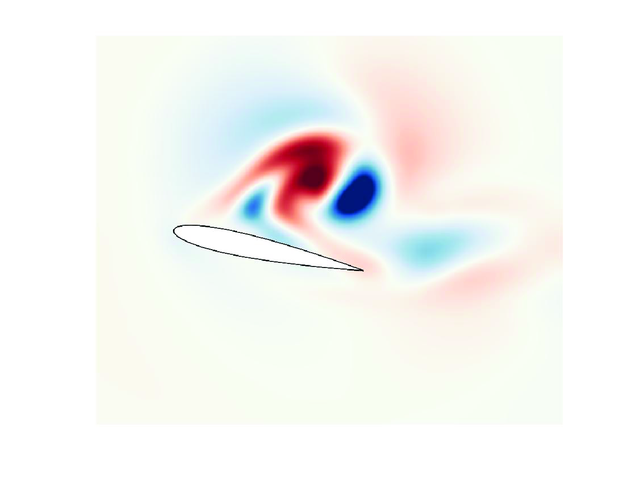
Around ${\tau }=-0.5$
, the vortical gust advects towards the leading edge of the airfoil. The primary amplified region, highlighted by dominant spatial modes, appears around the top boundary layer near the leading edge of the airfoil. At the same time, the secondary amplified region emerges to coincide with the core of the vortical disturbance, shown upstream of the leading three OTD modes. Additionally, streamwise oscillations in the model structures appear for the higher-order modes 2 and 3. Therefore, during the period when the vortex approaches the airfoil, the primary amplified structure stems from the boundary layer near the leading edge of the airfoil and the subdominant sensitive regions correlate with the advection of the baseline vortical disturbance.
${\tau }=-0.5$
, the vortical gust advects towards the leading edge of the airfoil. The primary amplified region, highlighted by dominant spatial modes, appears around the top boundary layer near the leading edge of the airfoil. At the same time, the secondary amplified region emerges to coincide with the core of the vortical disturbance, shown upstream of the leading three OTD modes. Additionally, streamwise oscillations in the model structures appear for the higher-order modes 2 and 3. Therefore, during the period when the vortex approaches the airfoil, the primary amplified structure stems from the boundary layer near the leading edge of the airfoil and the subdominant sensitive regions correlate with the advection of the baseline vortical disturbance.
After the vortical gust impinges on the airfoil, the boundary layer separates and rolls up into an LEV. Around ${\tau }=0$
, modes 1 and 2 identify the amplification of perturbations colocated and corotating with the LEV, as indicated above the suction side of the airfoil in figure 5(a). During the LEV formation, perturbations can experience maximum amplification along the core of the LEV. As the centre of the vortical disturbance nears the half-chord position around the airfoil at
${\tau }=0$
, modes 1 and 2 identify the amplification of perturbations colocated and corotating with the LEV, as indicated above the suction side of the airfoil in figure 5(a). During the LEV formation, perturbations can experience maximum amplification along the core of the LEV. As the centre of the vortical disturbance nears the half-chord position around the airfoil at ${\tau }=0.5$
, the LEV grows and moves towards the trailing edge of the airfoil. During this time, the most amplified region extends and shifts in the streamwise direction while rotating with the core of the LEV. By
${\tau }=0.5$
, the LEV grows and moves towards the trailing edge of the airfoil. During this time, the most amplified region extends and shifts in the streamwise direction while rotating with the core of the LEV. By ${\tau }=1$
, the LEV in the base flow has detached from the airfoil. During this time, the primary OTD mode still follows the advection and rotation of the LEV, while the wake region behind the trailing edge of the airfoil becomes increasingly important due to the trailing-edge vortex sheet roll-up. This shows the transition of the most amplified flow structure from the LEV to the wake behind the airfoil.
${\tau }=1$
, the LEV in the base flow has detached from the airfoil. During this time, the primary OTD mode still follows the advection and rotation of the LEV, while the wake region behind the trailing edge of the airfoil becomes increasingly important due to the trailing-edge vortex sheet roll-up. This shows the transition of the most amplified flow structure from the LEV to the wake behind the airfoil.
By examining the singular values and energy amplifications, we identify the evolution of each OTD mode over time. Temporal changes of the corresponding singular values and energy amplifications $g_i(t)$
are presented in figures 5(b) and 5(c). The first OTD mode aligns with the most amplified direction during the evolution, associated with a large singular value of
$g_i(t)$
are presented in figures 5(b) and 5(c). The first OTD mode aligns with the most amplified direction during the evolution, associated with a large singular value of $O(100)$
. In figure 5(c), the maximum possible energy amplification
$O(100)$
. In figure 5(c), the maximum possible energy amplification $g_1(t)$
and the suboptimal energy amplifications
$g_1(t)$
and the suboptimal energy amplifications $g_2(t)$
and
$g_2(t)$
and $g_3(t)$
have an increasing trend before
$g_3(t)$
have an increasing trend before $\tau =0$
. The increasing energy amplifications indicate that the perturbations can undergo a large transient growth as the LEV is forming. After the LEV detaches from the airfoil body around
$\tau =0$
. The increasing energy amplifications indicate that the perturbations can undergo a large transient growth as the LEV is forming. After the LEV detaches from the airfoil body around ${\tau }=0.5$
, the optimal and suboptimal energy amplifications become twice their initial values, which uncovers that the perturbations can experience large amplification in the trailing-edge wakes. Later, at
${\tau }=0.5$
, the optimal and suboptimal energy amplifications become twice their initial values, which uncovers that the perturbations can experience large amplification in the trailing-edge wakes. Later, at ${\tau }=1$
, the third OTD mode shows growth in energy. This third OTD mode exhibits finer flow structures, indicative of its role in capturing more localized and higher-frequency dynamics within the flow field. As the interaction progresses, the observed increase in the energy growth of this mode suggests an amplification of these finer structures, likely driven by the development of small-scale instabilities and the transfer of energy from larger to smaller scales within the vortex–airfoil interaction.
${\tau }=1$
, the third OTD mode shows growth in energy. This third OTD mode exhibits finer flow structures, indicative of its role in capturing more localized and higher-frequency dynamics within the flow field. As the interaction progresses, the observed increase in the energy growth of this mode suggests an amplification of these finer structures, likely driven by the development of small-scale instabilities and the transfer of energy from larger to smaller scales within the vortex–airfoil interaction.

Figure 6. (a) Vorticity fields of the time-varying base flow and the top three OTD vorticity modes, (b) the leading three singular values and (c) the leading three energy amplifications for $G=1$
.
$G=1$
.
Now, let us consider the impact of vortex strength on the transient amplification of perturbations. In the case of a disturbed flow with a strong positive vortical gust of $G=1$
, the vorticity field undergoes prominent transient fluctuations, as shown in figure 6(ai). The dominant three spatial time-dependent modes are also presented. Around
$G=1$
, the vorticity field undergoes prominent transient fluctuations, as shown in figure 6(ai). The dominant three spatial time-dependent modes are also presented. Around ${\tau }=-0.5$
, the strong vortex induces drastic deformation of the vortex sheet around the leading edge of the airfoil. During this time, the primary and secondary modes exhibit substantial amplification potential of perturbations in a localized region concentrated on the core of the vortex roll-up. Shortly after
${\tau }=-0.5$
, the strong vortex induces drastic deformation of the vortex sheet around the leading edge of the airfoil. During this time, the primary and secondary modes exhibit substantial amplification potential of perturbations in a localized region concentrated on the core of the vortex roll-up. Shortly after ${\tau }=0$
, the strong dipole (vortex pair) forms over the airfoil surface. The core of the negative LEV emerges as the most amplified region shown in modes 1 and 2. Mode 3 highlights a thin region between the positive vortex and the negative vortex in the LEV pair, suggesting that the stretching of vortex filaments within the LEV can lead to the growth of perturbations.
${\tau }=0$
, the strong dipole (vortex pair) forms over the airfoil surface. The core of the negative LEV emerges as the most amplified region shown in modes 1 and 2. Mode 3 highlights a thin region between the positive vortex and the negative vortex in the LEV pair, suggesting that the stretching of vortex filaments within the LEV can lead to the growth of perturbations.
Later, when the vortex pair detaches from the airfoil after ${\tau }=0.5$
, all three dominant OTD modes identify the vortex pair as the most amplified flow structure. Concurrently, a small positive vortical structure in the base flow emerges at the trailing edge around
${\tau }=0.5$
, all three dominant OTD modes identify the vortex pair as the most amplified flow structure. Concurrently, a small positive vortical structure in the base flow emerges at the trailing edge around ${\tau }=0.5$
. The amplified region behind the trailing edge suggests that a secondary amplification of the perturbations is associated with the formation of a trailing-edge vortex. From the analysis of the OTD modes over time, we find that the most amplified flow structures follow the vortices induced during the interaction between the strong vortical gust and the airfoil. The LEV pair, being a focal point of energy concentration, coincides with the maximum amplification regions of the OTD modes. The dominant singular values and the energy amplifications over time are shown in figure 6(b–c). Across all three modes, singular values exhibit a steady increase from
${\tau }=0.5$
. The amplified region behind the trailing edge suggests that a secondary amplification of the perturbations is associated with the formation of a trailing-edge vortex. From the analysis of the OTD modes over time, we find that the most amplified flow structures follow the vortices induced during the interaction between the strong vortical gust and the airfoil. The LEV pair, being a focal point of energy concentration, coincides with the maximum amplification regions of the OTD modes. The dominant singular values and the energy amplifications over time are shown in figure 6(b–c). Across all three modes, singular values exhibit a steady increase from ${\tau }=-1$
to
${\tau }=-1$
to $1$
. The optimal energy amplification is approximately seven times its initial value, revealing that perturbations can be continuously amplified during the interaction between the vortex and the wing. The second and third energy growths are non-monotonic, suggesting that the higher-order modes have different temporal growth rates compared with the first mode.
$1$
. The optimal energy amplification is approximately seven times its initial value, revealing that perturbations can be continuously amplified during the interaction between the vortex and the wing. The second and third energy growths are non-monotonic, suggesting that the higher-order modes have different temporal growth rates compared with the first mode.
In contrast, when encountering a negative vortical gust, the dynamics of perturbations differ from those cases of positive vortex–airfoil interactions. We employ OTD mode analysis for the unsteady base flow concerning interactions between an airfoil and a moderate vortical gust ( $G=-0.5$
). Despite inducing significant lift and drag fluctuations on the airfoil, a moderate negative gust does not lead to large vortex shedding upon impingement, as visualized in figure 7(a). Regarding the perturbation amplification, the primary OTD mode only exhibits a gradual change in the most amplified flow structures. The amplified regions identified by mode 1 are associated with the deformation of the wakes from
$G=-0.5$
). Despite inducing significant lift and drag fluctuations on the airfoil, a moderate negative gust does not lead to large vortex shedding upon impingement, as visualized in figure 7(a). Regarding the perturbation amplification, the primary OTD mode only exhibits a gradual change in the most amplified flow structures. The amplified regions identified by mode 1 are associated with the deformation of the wakes from ${\tau }=-0.5$
to 1.
${\tau }=-0.5$
to 1.

Figure 7. (a) Vorticity fields of the time-varying base flow and the top three OTD vorticity modes, (b) the leading three singular values and (c) the leading three energy amplifications for $G=-0.5$
.
$G=-0.5$
.

Figure 8. (a) Vorticity fields of the time-varying base flow and the top three OTD vorticity modes, (b) the leading three singular values and (c) the leading three energy amplifications for $G=-1$
.
$G=-1$
.
The time evolution of the amplified regions in modes 2 and 3 exhibits different perturbation dynamics from mode 1. Before ${\tau }=-0.5$
, modes 2 and 3 do not exhibit any prominent features in spatially sensitive areas. As the moderate negative vortex interacts with the airfoil around
${\tau }=-0.5$
, modes 2 and 3 do not exhibit any prominent features in spatially sensitive areas. As the moderate negative vortex interacts with the airfoil around ${\tau }=0$
, the boundary layer separates from the pressure side of the airfoil and becomes highlighted by OTD modes 2 and 3. Subsequently, as the vortical gust advects downstream after
${\tau }=0$
, the boundary layer separates from the pressure side of the airfoil and becomes highlighted by OTD modes 2 and 3. Subsequently, as the vortical gust advects downstream after ${\tau }=0.5$
, a compact amplified area from the bottom side vortex sheet roll-up is captured in the second and third modes. This result suggests that the second and third modes are more sensitive to localized disturbances and transient phenomena. This underscores the importance of higher-order modes in providing a comprehensive understanding of the vortex–airfoil interaction, particularly in capturing the nuanced flow features that govern the local perturbation behaviour.
${\tau }=0.5$
, a compact amplified area from the bottom side vortex sheet roll-up is captured in the second and third modes. This result suggests that the second and third modes are more sensitive to localized disturbances and transient phenomena. This underscores the importance of higher-order modes in providing a comprehensive understanding of the vortex–airfoil interaction, particularly in capturing the nuanced flow features that govern the local perturbation behaviour.
The corresponding singular values and perturbation amplifications are shown in figure 7(b–c). The leading singular value $\sigma _1=O(100)$
remains fairly flat during its evolution, corresponding to the gradual changes of the leading OTD mode. On the other hand, the secondary energy amplification
$\sigma _1=O(100)$
remains fairly flat during its evolution, corresponding to the gradual changes of the leading OTD mode. On the other hand, the secondary energy amplification $g_2(t)$
shows a spike around
$g_2(t)$
shows a spike around ${\tau }=-0.1$
, as depicted in figure 7(c). The large energy amplification of mode 2 indicates that the perturbations can grow large when the bottom side vortex sheet starts to roll up. The ability of the second mode to detect and amplify during the onset of roll-up underscores its importance in tracking the timing of transient perturbation amplification. Eventually all three energy amplifications become lower than 1 at
${\tau }=-0.1$
, as depicted in figure 7(c). The large energy amplification of mode 2 indicates that the perturbations can grow large when the bottom side vortex sheet starts to roll up. The ability of the second mode to detect and amplify during the onset of roll-up underscores its importance in tracking the timing of transient perturbation amplification. Eventually all three energy amplifications become lower than 1 at $\tau =1$
, suggesting a loss of coherent structures and a decrease in the energy of the OTD modes.
$\tau =1$
, suggesting a loss of coherent structures and a decrease in the energy of the OTD modes.
Let us now consider the interactions between a strong negative vortical gust ( $G=-1$
) and an airfoil, which inherently include high levels of unsteadiness and nonlinearity. As visualized in figure 8(a), a large vortex pair is generated from the pressure side of the airfoil around
$G=-1$
) and an airfoil, which inherently include high levels of unsteadiness and nonlinearity. As visualized in figure 8(a), a large vortex pair is generated from the pressure side of the airfoil around ${\tau }=0$
during the violent interaction. After the vortex pair detaches from the airfoil body around
${\tau }=0$
during the violent interaction. After the vortex pair detaches from the airfoil body around ${\tau }=1$
, a smaller LEV is generated from the vortex sheet roll-up on the suction side of the airfoil. The three dominant modes in general highlight the most amplified region following the large vortex pair below the airfoil, shown in figure 8(a). Modes 1–3 have similar modal structures with notable features about the positive vortex. The most amplified structures coincide with the motion and rotation of the vortex pair that is generated around
${\tau }=1$
, a smaller LEV is generated from the vortex sheet roll-up on the suction side of the airfoil. The three dominant modes in general highlight the most amplified region following the large vortex pair below the airfoil, shown in figure 8(a). Modes 1–3 have similar modal structures with notable features about the positive vortex. The most amplified structures coincide with the motion and rotation of the vortex pair that is generated around ${\tau }=0$
. In addition, a secondary sensitive region is found to be related to the subsequent vortex roll-up above the airfoil, as indicated by the emerging spatial structures about the LEV around
${\tau }=0$
. In addition, a secondary sensitive region is found to be related to the subsequent vortex roll-up above the airfoil, as indicated by the emerging spatial structures about the LEV around ${\tau }=1$
.
${\tau }=1$
.
In figure 8(b,c), the variations of the three leading singular values and energy amplifications show that the amplification of perturbations generally becomes larger over $-1 \le {\tau } \le 1$
. In this case, the interaction between the strong negative vortex and the airfoil gives rise to a high level of perturbation amplifications. The suboptimal energy amplification
$-1 \le {\tau } \le 1$
. In this case, the interaction between the strong negative vortex and the airfoil gives rise to a high level of perturbation amplifications. The suboptimal energy amplification $g_2(t)$
exhibits one peak around
$g_2(t)$
exhibits one peak around ${\tau }=-0.1$
, as shown in the figure 8(c). During this time, both the positive and negative vorticity on the bottom side of the airfoil are highlighted by OTD mode 2. This result suggests that the perturbations can be amplified both in the LEV and the strong disturbance vortex. Later when the LEV convects into the wake near the airfoil trailing edge, the optimal energy amplification
${\tau }=-0.1$
, as shown in the figure 8(c). During this time, both the positive and negative vorticity on the bottom side of the airfoil are highlighted by OTD mode 2. This result suggests that the perturbations can be amplified both in the LEV and the strong disturbance vortex. Later when the LEV convects into the wake near the airfoil trailing edge, the optimal energy amplification $g_1(t)$
becomes four times its initial value during evolution, as presented in figure 8(c). The increasing trend of energy growth indicates a substantial amplification of perturbations.
$g_1(t)$
becomes four times its initial value during evolution, as presented in figure 8(c). The increasing trend of energy growth indicates a substantial amplification of perturbations.
The uncovering of optimal time-dependent modes offers valuable insights for understanding transient amplification in response to perturbations about unsteady flows. By leveraging the most amplified structures discovered by OTD mode analysis, we can pinpoint the most amplified regions subject to time-varying perturbations. For a moderate positive vortex–airfoil interaction case ( $G=0.5$
), OTD modes unveil complex transitions of amplified flow structures from the LEV sheet to the forming LEV, with a secondary sensitive region as the wakes behind the airfoil. On the other hand, the leading amplified structures evolve slowly when the airfoil encounters a moderate negative vortical gust (
$G=0.5$
), OTD modes unveil complex transitions of amplified flow structures from the LEV sheet to the forming LEV, with a secondary sensitive region as the wakes behind the airfoil. On the other hand, the leading amplified structures evolve slowly when the airfoil encounters a moderate negative vortical gust ( $G=-0.5$
). When the airflow is disturbed by a strong vortex (
$G=-0.5$
). When the airflow is disturbed by a strong vortex ( $G=\pm 1$
), OTD modes expose a direct correlation between shedding vortex trajectory and transient amplification of perturbations.
$G=\pm 1$
), OTD modes expose a direct correlation between shedding vortex trajectory and transient amplification of perturbations.
The energy amplification of OTD modes provides valuable insights into the underlying dynamics that govern the evolution of perturbations. A monotonic increase in energy amplification, as seen in $g_1(t)$
ofthe
$g_1(t)$
ofthe $G=\pm 1$
cases, indicates a persistent instability mechanism. This mechanism for these two vortex–airfoil interactions is correlated with the high intensity of the vorticity of the primary shedding vortex. However, the region with the highest amplification is not always associated with the largest vorticity magnitude. For the example of
$G=\pm 1$
cases, indicates a persistent instability mechanism. This mechanism for these two vortex–airfoil interactions is correlated with the high intensity of the vorticity of the primary shedding vortex. However, the region with the highest amplification is not always associated with the largest vorticity magnitude. For the example of $G=-0.5$
, the highlighted modal structures of all three leading modes do not collapse on the leading edge of the airfoil where the highest vorticity magnitude is observed. Diverse transient behaviours are uncovered by the variations of energy amplification. For example,
$G=-0.5$
, the highlighted modal structures of all three leading modes do not collapse on the leading edge of the airfoil where the highest vorticity magnitude is observed. Diverse transient behaviours are uncovered by the variations of energy amplification. For example, $g_1$
and
$g_1$
and $g_2$
exhibit rapid increases followed by decreases, as shown in figure 5. A rapid increase in energy amplification indicates a highly unstable region of the flow. The roll-up of the LEV for
$g_2$
exhibit rapid increases followed by decreases, as shown in figure 5. A rapid increase in energy amplification indicates a highly unstable region of the flow. The roll-up of the LEV for $G=0.5$
corresponds to increasing energy amplifications. This region is prone to perturbations that can quickly amplify and lead to significant flow modifications. The subsequent decay suggests that the instability is transient, energy can be transferred downstream because of the wake formation.
$G=0.5$
corresponds to increasing energy amplifications. This region is prone to perturbations that can quickly amplify and lead to significant flow modifications. The subsequent decay suggests that the instability is transient, energy can be transferred downstream because of the wake formation.
The OTD mode analysis can be used to identify perturbation dynamics for more complex flows, such as extreme aerodynamic flows and turbulent flows. Capturing the coherent structures that are receptive to perturbations in a time-evolving manner is critical in understanding the unsteady flow physics. In addition, OTD mode analysis has the potential to guide flow control strategies. The OTD modes evolve dynamically, identifying when and where perturbations are most likely to grow. The OTD modes inform when the flow is most receptive to perturbations, suggesting that actuators or energy inputs (e.g. actuation via jets or local forcing) can be applied at the most effective moments to amplify (or suppress) instabilities. For example, for the $G=0.5$
case, when the vortex is approaching the airfoil, the most amplified region is the leading edge of the airfoil. The control effects at this moment should focus on the local region around the leading edge. On the other hand, when the vortex convects to the trailing edge of the airfoil, the trailing edge can be amplified more compared with the leading edge. A different local forcing near the trailing edge will be more efficient than the leading edge at this specific moment.
$G=0.5$
case, when the vortex is approaching the airfoil, the most amplified region is the leading edge of the airfoil. The control effects at this moment should focus on the local region around the leading edge. On the other hand, when the vortex convects to the trailing edge of the airfoil, the trailing edge can be amplified more compared with the leading edge. A different local forcing near the trailing edge will be more efficient than the leading edge at this specific moment.
5. Conclusions
Vortex–airfoil interactions involve strong transient features, which are difficult to characterize with classical methods that are founded on time-invariant or periodic flow. In this study, OTD mode analysis was used to identify the most amplified flow structures of unsteady base flows of vortex–airfoil interactions. We considered four scenarios of vortex–airfoil interaction with a moderate positive vortex ( $G=0.5$
), a strong positive vortex (
$G=0.5$
), a strong positive vortex ( $G=1$
), a moderate negative vortex (
$G=1$
), a moderate negative vortex ( $G=-0.5$
) and a strong negative vortex (
$G=-0.5$
) and a strong negative vortex ( $G=-1$
). The OTD modes capture the most amplified regions subject to perturbations, and the singular value variations offer insights into the significance of the OTD modes. For the vortex–airfoil interaction of
$G=-1$
). The OTD modes capture the most amplified regions subject to perturbations, and the singular value variations offer insights into the significance of the OTD modes. For the vortex–airfoil interaction of $G=0.5$
, the amplified region transitions from the LEV sheet to the evolving LEV. In addition, a secondary amplified flow structure near the trailing-edge wake is revealed by subdominant OTD modes. When a strong positive vortical gust (
$G=0.5$
, the amplified region transitions from the LEV sheet to the evolving LEV. In addition, a secondary amplified flow structure near the trailing-edge wake is revealed by subdominant OTD modes. When a strong positive vortical gust ( $G=1$
) interacts with an airfoil, perturbations are amplified following the advection and rotation of the LEV pair generated from the impingement of the strong vortical gust. For a moderate negative vortex disturbance (G = –0.5), the flowfield exhibits few dominant vortical structures, and thus, the dominant OTD mode follows the advection of the wakes around the airfoil and undergoes gradual changes over time. For the strong negative vortex–airfoil interaction of
$G=1$
) interacts with an airfoil, perturbations are amplified following the advection and rotation of the LEV pair generated from the impingement of the strong vortical gust. For a moderate negative vortex disturbance (G = –0.5), the flowfield exhibits few dominant vortical structures, and thus, the dominant OTD mode follows the advection of the wakes around the airfoil and undergoes gradual changes over time. For the strong negative vortex–airfoil interaction of $G=-1$
, the shedding vortex pair convecting from the pressure side of the airfoil surface is identified as the most amplified flow structure subject to perturbations. The findings through the OTD mode analysis for the present vortex–gust airfoil interactions provide insights into the transient amplification of perturbations in unsteady flight conditions and hold promising implications for diverse unsteady flow problems.
$G=-1$
, the shedding vortex pair convecting from the pressure side of the airfoil surface is identified as the most amplified flow structure subject to perturbations. The findings through the OTD mode analysis for the present vortex–gust airfoil interactions provide insights into the transient amplification of perturbations in unsteady flight conditions and hold promising implications for diverse unsteady flow problems.
Acknowledgments
Y.Z. and K.T. acknowledge the support from the US Air Force Office of Scientific Research (grant no. FA 9550-21- 1-0178) and the US Department of Defense Vannevar Bush Faculty Fellowship (grant no. N 00014-22- 1-2798).
Declaration of interest
The authors report no conflict of interest.
Appendix A. Verification of OTD modes
The OTD modes are obtained by time-integrating the evolution (2.13). In this appendix, we briefly outline the checks performed to ensure the accuracy of the OTD modes. We first check the temporal convergence of the top three singular values, as shown in figure 9 for the case of $G=-0.5$
. Using different time step sizes of
$G=-0.5$
. Using different time step sizes of $\Delta \tau =8.5\times {10}^{-5}$
and
$\Delta \tau =8.5\times {10}^{-5}$
and $1.7\times {10}^{-4}$
, the singular values from the two cases match well with each other over time. Therefore, we choose
$1.7\times {10}^{-4}$
, the singular values from the two cases match well with each other over time. Therefore, we choose $\Delta \tau =1.7\times {10}^{-4}$
as the default time step for finding the OTD modes.
$\Delta \tau =1.7\times {10}^{-4}$
as the default time step for finding the OTD modes.

Figure 9. Time convergence on the top three singular values of moderate negative vortex–airfoil interaction.
Next, we examine the convergence on the number of OTD modes $r$
. This is studied by comparing the singular values for different numbers of modes
$r$
. This is studied by comparing the singular values for different numbers of modes $r$
. For brevity, we present only positive vortex–airfoil interaction cases in the following analyses. The negative vortex–airfoil interaction cases exhibit analogous results. As presented in figure 10 for positive gust cases, the top five singular values over time are shown for
$r$
. For brevity, we present only positive vortex–airfoil interaction cases in the following analyses. The negative vortex–airfoil interaction cases exhibit analogous results. As presented in figure 10 for positive gust cases, the top five singular values over time are shown for $r=5, 15$
and
$r=5, 15$
and $40$
. The solid lines represent the
$40$
. The solid lines represent the $r=40$
cases, the dashed lines denote the
$r=40$
cases, the dashed lines denote the $r=15$
cases and the dashed–dot lines are the
$r=15$
cases and the dashed–dot lines are the $r=5$
cases. In general, the leading three singular values of cases with different numbers of modes agree perfectly with each other. However, the lowest
$r=5$
cases. In general, the leading three singular values of cases with different numbers of modes agree perfectly with each other. However, the lowest $r=5$
cases have discrepancies in the fourth and fifth singular values compared with cases with a larger number of modes. Hence, we concluded that the singular values exhibit convergence with 15 modes for positive vortex–airfoil interaction cases.
$r=5$
cases have discrepancies in the fourth and fifth singular values compared with cases with a larger number of modes. Hence, we concluded that the singular values exhibit convergence with 15 modes for positive vortex–airfoil interaction cases.

Figure 10. Convergence on the number of OTD modes for the top five singular values of four disturbed flow cases: $(a)$
$(a)$ $G=0.5$
,
$G=0.5$
, $(b)$
$(b)$ $G=1$
.
$G=1$
.
The convergence check on the number of modes is also performed by comparing the cosine similarity between modes. Cosine similarity is defined as the inner product of two vectors, whose absolute value is in the range of $[0,1]$
. When the absolute cosine similarity approaches 1, it indicates that the two vectors are similar to each other. For convenience, we present the absolute value of the cosine similarity between OTD modes below. We examine the cosine similarity of the dominant three modes betweenthe
$[0,1]$
. When the absolute cosine similarity approaches 1, it indicates that the two vectors are similar to each other. For convenience, we present the absolute value of the cosine similarity between OTD modes below. We examine the cosine similarity of the dominant three modes betweenthe $r=5$
and
$r=5$
and $15$
cases. Figures 11(a) and 11(b) show the vortex–airfoil interaction cases for positive vortices, respectively. Among the comparisons of positive vortex cases of
$15$
cases. Figures 11(a) and 11(b) show the vortex–airfoil interaction cases for positive vortices, respectively. Among the comparisons of positive vortex cases of $G=0.5$
and
$G=0.5$
and $1$
, all three modes from the
$1$
, all three modes from the $r=5$
cases achieve over 99.99
$r=5$
cases achieve over 99.99 $\%$
cosine similarity with the corresponding modes from
$\%$
cosine similarity with the corresponding modes from $r=15$
cases. The high similarity levels demonstrate the high agreement of the leading three modes extracted from disturbed flow scenarios. With only
$r=15$
cases. The high similarity levels demonstrate the high agreement of the leading three modes extracted from disturbed flow scenarios. With only $r=5$
modes, the top three modes are as accurate as using 15 modes.
$r=5$
modes, the top three modes are as accurate as using 15 modes.

Figure 11. Cosine similarity of each of the three dominant modes between $r=5$
and
$r=5$
and $r=15$
of positive vortex–airfoil interaction cases.
$r=15$
of positive vortex–airfoil interaction cases.

Figure 12. The influence of initial time for OTD evolution. For each of the leading three OTD modes, cosine similarity is checked between modes computed with initial time $\tau _0=-0.85$
and
$\tau _0=-0.85$
and $-1$
(solid lines), and between
$-1$
(solid lines), and between $\tau _0=-1.12$
and
$\tau _0=-1.12$
and $-1$
(dashed lines). The initial condition matrix is extracted from the flow state snapshots over
$-1$
(dashed lines). The initial condition matrix is extracted from the flow state snapshots over $[\tau _a,\tau _b]\in [-1,-0.4]$
.
$[\tau _a,\tau _b]\in [-1,-0.4]$
.
Now we investigate the influence of initial evolution time $\tau _0$
on the OTD modes, the leading singular values converge while being insensitive to the choice of the OTD initial condition time
$\tau _0$
on the OTD modes, the leading singular values converge while being insensitive to the choice of the OTD initial condition time $\tau _0$
. Using the same initial condition matrix considering
$\tau _0$
. Using the same initial condition matrix considering $[\tau _a,\tau _b]=[-1,-0.4]$
, we integrate the initial OTD modes from different initial times of
$[\tau _a,\tau _b]=[-1,-0.4]$
, we integrate the initial OTD modes from different initial times of $\tau _0=-1.12$
,
$\tau _0=-1.12$
, $-1$
and
$-1$
and $-0.85$
. The influence of different initial times on the evolution of the leading three modes is presented in figure 12. The solid lines indicate the comparison of each of the leading three modes computed with
$-0.85$
. The influence of different initial times on the evolution of the leading three modes is presented in figure 12. The solid lines indicate the comparison of each of the leading three modes computed with $\tau _0=-0.85$
and
$\tau _0=-0.85$
and $-1$
, and the dashed lines are computed with
$-1$
, and the dashed lines are computed with $\tau _0=-1.12$
and
$\tau _0=-1.12$
and $-1$
. In the case of
$-1$
. In the case of $G=0.5$
, each of the three dominant modes with different initial evolution moments maintains over 80
$G=0.5$
, each of the three dominant modes with different initial evolution moments maintains over 80 $\%$
similarity throughout the entire time span. For the vortex–airfoil interaction cases of
$\%$
similarity throughout the entire time span. For the vortex–airfoil interaction cases of $G=1$
, however, the similarities start from relatively low values and increase afterward. This indicates that the observed dominant features converge to the same subset of OTD modes regardless of the initial evolution moments. Based on these results, we perform the OTD mode evolution from
$G=1$
, however, the similarities start from relatively low values and increase afterward. This indicates that the observed dominant features converge to the same subset of OTD modes regardless of the initial evolution moments. Based on these results, we perform the OTD mode evolution from $\tau _0=-1$
, and the initial condition is given by
$\tau _0=-1$
, and the initial condition is given by $[\tau _a,\tau _b]=[-1,-0.4]$
.
$[\tau _a,\tau _b]=[-1,-0.4]$
.

Figure 13. The evolution of OTD modes with random noise as the initial condition, $G=0.5$
.
$G=0.5$
.
To show that the primary OTD mode shown earlier in figure 5 is not dependent on the initial condition, let us also consider random noise as the initial condition and evolve the OTD modes in time for the $G=0.5$
case. We use 15 orthonormal random noise vectors as the initial OTD modes at
$G=0.5$
case. We use 15 orthonormal random noise vectors as the initial OTD modes at ${\tau }=-1$
.
${\tau }=-1$
.
As shown in the figure 13, the OTD mode 1 captures very similar structures to the case shown in the figure 5 when ${\tau }\gt 0$
. The amplified region starts from the LEV sheet around
${\tau }\gt 0$
. The amplified region starts from the LEV sheet around ${\tau }=-0.5$
, then evolves with the shedding of the LEV. Later around
${\tau }=-0.5$
, then evolves with the shedding of the LEV. Later around ${\tau }=1$
, the region after the trailing edge of the airfoil is highlighted as the most amplified region. On the other hand, OTD modes 2 and 3 are filled with random noises evolved from the initial condition. The noise structures get smoothed out as time increases, and vortical structures similar to OTD mode 1 are observed near the airfoil.
${\tau }=1$
, the region after the trailing edge of the airfoil is highlighted as the most amplified region. On the other hand, OTD modes 2 and 3 are filled with random noises evolved from the initial condition. The noise structures get smoothed out as time increases, and vortical structures similar to OTD mode 1 are observed near the airfoil.
Compared with the initial modes, which are the singular vectors from the initial perturbation matrix, random noise as the initial condition yields a worse result in capturing the perturbation amplification. Although the OTD modes converge to the most amplified structures subject to perturbations, the convergence requires a large number of initial condition vectors. Therefore, we infer that a proper set of initial OTD modes can be selected from the SVD of the initial condition matrix collected around the OTD evolution starting time.
Appendix B. Most amplified initial perturbation
After acquiring knowledge about transient amplifications from spatial modes, we can identify which perturbation has the maximum impact on the disturbed flows. This information is crucial for understanding the underlying mechanisms driving flow instabilities and transient growth phenomena. The optimal initial perturbation that leads to the maximum amplification at time $\tau ^*$
is obtained via (2.18). Starting from
$\tau ^*$
is obtained via (2.18). Starting from $\tau _0$
to
$\tau _0$
to $\tau ^*$
, the most amplified initial perturbation can be written as
$\tau ^*$
, the most amplified initial perturbation can be written as
 \begin{equation} {\boldsymbol{\mathsf{q}}}_0^{\prime *}={\boldsymbol{\hat{\mathsf{U}}}}_r(\tau _0){\boldsymbol {\Sigma }}_r(\tau _0){\boldsymbol{\hat{\mathsf{Y}}}}_r^{\textrm {T}}(\tau _0){\boldsymbol{\hat{\mathsf{y}}}}_1(\tau ^{*})\in {\mathbb {R}}^{n}, \end{equation}
which leads to a largest singular value at $\sigma _1(\tau ^*)$
by evolving
$\sigma _1(\tau ^*)$
by evolving ${\boldsymbol{\mathsf{q}}}_0^{\prime *}$
in OTD subspace from
${\boldsymbol{\mathsf{q}}}_0^{\prime *}$
in OTD subspace from $\tau _0$
to
$\tau _0$
to $\tau ^*$
. It is important to note that the optimal initial condition determined via B1) is confined to the space spanned by the columns of
$\tau ^*$
. It is important to note that the optimal initial condition determined via B1) is confined to the space spanned by the columns of ${\boldsymbol{\mathsf{Q}}}^{\prime}_0 \approx {\boldsymbol{\hat{\mathsf{U}}}}_r(\tau _0){\boldsymbol {\Sigma }}_r(\tau _0){\boldsymbol{\hat{\mathsf{Y}}}}_r^{\textrm {T}}(\tau _0)$
.
${\boldsymbol{\mathsf{Q}}}^{\prime}_0 \approx {\boldsymbol{\hat{\mathsf{U}}}}_r(\tau _0){\boldsymbol {\Sigma }}_r(\tau _0){\boldsymbol{\hat{\mathsf{Y}}}}_r^{\textrm {T}}(\tau _0)$
.

Figure 14. Evolution of the leading singular value subject to different ${\boldsymbol{\mathsf{q}}}_0^{\prime *}$
at
${\boldsymbol{\mathsf{q}}}_0^{\prime *}$
at $\tau _0 = -1, -0.5, 0,$
and
$\tau _0 = -1, -0.5, 0,$
and $0.5$
(shown with circles),
$0.5$
(shown with circles), $\tau ^*=1$
(square). The vorticity fields surrounded by yellow, purple and green dashed boxes indicate the most amplified initial perturbations at
$\tau ^*=1$
(square). The vorticity fields surrounded by yellow, purple and green dashed boxes indicate the most amplified initial perturbations at $\tau _0= -0.5, 0,$
and 0.5, respectively. Each perturbation is normalized for visualization.
$\tau _0= -0.5, 0,$
and 0.5, respectively. Each perturbation is normalized for visualization.
To show the most amplified perturbation at different $\tau _0$
that arrives at the largest singular value at
$\tau _0$
that arrives at the largest singular value at $\tau ^*=1$
, we compare its singular value with the largest singular value from the evolution of the set of perturbations
$\tau ^*=1$
, we compare its singular value with the largest singular value from the evolution of the set of perturbations ${{\boldsymbol{\mathsf{Q}}}}_r^{\prime }\equiv {\boldsymbol{\hat{\mathsf{U}}}}_r(\tau _0=-1){\boldsymbol {\Sigma }}_r(\tau _0=-1){\boldsymbol{\hat{\mathsf{Y}}}}_r^{\textrm {T}}(\tau _0=-1)$
in the OTD subspace. The product of the OTD modes and the associated coefficients approximates the evolution of the set of perturbations
${{\boldsymbol{\mathsf{Q}}}}_r^{\prime }\equiv {\boldsymbol{\hat{\mathsf{U}}}}_r(\tau _0=-1){\boldsymbol {\Sigma }}_r(\tau _0=-1){\boldsymbol{\hat{\mathsf{Y}}}}_r^{\textrm {T}}(\tau _0=-1)$
in the OTD subspace. The product of the OTD modes and the associated coefficients approximates the evolution of the set of perturbations ${{\boldsymbol{\mathsf{Q}}}}_r^{\prime }$
, which is referred to as the baseline case in this section. We present the leading singular value of evolving
${{\boldsymbol{\mathsf{Q}}}}_r^{\prime }$
, which is referred to as the baseline case in this section. We present the leading singular value of evolving ${{\boldsymbol{\mathsf{Q}}}}_r^{\prime }$
over time with blue solid lines in figure 14. Starting from four initial conditions at
${{\boldsymbol{\mathsf{Q}}}}_r^{\prime }$
over time with blue solid lines in figure 14. Starting from four initial conditions at $\tau _0= -1, -0.5, 0$
and
$\tau _0= -1, -0.5, 0$
and $0.5$
, the most amplified initial perturbations are identified from
$0.5$
, the most amplified initial perturbations are identified from ${\boldsymbol{\mathsf{q}}}_0^{\prime *}={\boldsymbol{\hat{\mathsf{U}}}}_r(\tau _0){\boldsymbol {\Sigma }}_r(\tau _0){\boldsymbol{\hat{\mathsf{Y}}}}_r^{\textrm {T}}(\tau _0){\boldsymbol{\hat{\mathsf{y}}}}_1(\tau ^{*}=1)$
. The singular value variations are shown on the left-hand side of figure 14. For the vortex–airfoil interaction cases of
${\boldsymbol{\mathsf{q}}}_0^{\prime *}={\boldsymbol{\hat{\mathsf{U}}}}_r(\tau _0){\boldsymbol {\Sigma }}_r(\tau _0){\boldsymbol{\hat{\mathsf{Y}}}}_r^{\textrm {T}}(\tau _0){\boldsymbol{\hat{\mathsf{y}}}}_1(\tau ^{*}=1)$
. The singular value variations are shown on the left-hand side of figure 14. For the vortex–airfoil interaction cases of $G=\pm 0.5$
, the singular values from
$G=\pm 0.5$
, the singular values from ${\boldsymbol{\mathsf{q}}}_0^{\prime *}(\tau _0= -1, -0.5, 0)$
and
${\boldsymbol{\mathsf{q}}}_0^{\prime *}(\tau _0= -1, -0.5, 0)$
and ${\boldsymbol{\mathsf{q}}}_0^{\prime *}(\tau _0= 0.5)$
almost collapse with the leading singular value of evolving the full set of perturbations
${\boldsymbol{\mathsf{q}}}_0^{\prime *}(\tau _0= 0.5)$
almost collapse with the leading singular value of evolving the full set of perturbations ${{\boldsymbol{\mathsf{Q}}}}_r^{\prime }$
. This result reveals that there exists one single perturbation that can be amplified the most over time. On the other hand, it is observed that the most amplified initial perturbations from cases of
${{\boldsymbol{\mathsf{Q}}}}_r^{\prime }$
. This result reveals that there exists one single perturbation that can be amplified the most over time. On the other hand, it is observed that the most amplified initial perturbations from cases of $G=\pm 1$
have lower singular values than the largest singular value of the baseline case. This suggests that a strong vortex–airfoil interaction The normalized
$G=\pm 1$
have lower singular values than the largest singular value of the baseline case. This suggests that a strong vortex–airfoil interaction The normalized ${\boldsymbol{\mathsf{q}}}_0^{\prime *}$
subject to different
${\boldsymbol{\mathsf{q}}}_0^{\prime *}$
subject to different $\tau _0$
are shown on the right-hand side of figure 14. For all interaction cases, they follow a similar shape of the leading mode
$\tau _0$
are shown on the right-hand side of figure 14. For all interaction cases, they follow a similar shape of the leading mode $\hat{\boldsymbol{\mathsf{u}}}_1(t)$
, indicating that the regions in which perturbation is amplified the most can be captured by the leading OTD mode.
$\hat{\boldsymbol{\mathsf{u}}}_1(t)$
, indicating that the regions in which perturbation is amplified the most can be captured by the leading OTD mode.

Figure 15. Evolution of the leading singular value subject to different ${\boldsymbol{\mathsf{q}}}_0^{\prime *}$
at
${\boldsymbol{\mathsf{q}}}_0^{\prime *}$
at $\tau ^* = \tau ^{*}(\sigma _{{max}}), -0.5, 0,$
and
$\tau ^* = \tau ^{*}(\sigma _{{max}}), -0.5, 0,$
and $0.5$
(denoted as squares) with
$0.5$
(denoted as squares) with $\tau _0=-1$
. The vorticity fields surrounded by orange, green and grey dashed boxes indicate the most amplified perturbations at
$\tau _0=-1$
. The vorticity fields surrounded by orange, green and grey dashed boxes indicate the most amplified perturbations at $\tau ^*= \tau ^*(\sigma _{{{max}}}), -0.5,$
and the difference between them, respectively. Each perturbation is normalized for visualization.
$\tau ^*= \tau ^*(\sigma _{{{max}}}), -0.5,$
and the difference between them, respectively. Each perturbation is normalized for visualization.
Moreover, figure 15 presents the most amplified perturbations for a fixed $\tau _0$
and different
$\tau _0$
and different $\tau ^*$
. The initial evolution time are the same at
$\tau ^*$
. The initial evolution time are the same at $\tau _0=-1$
, and the target singular values are at
$\tau _0=-1$
, and the target singular values are at $\tau ^*=\tau ^{*}(\sigma _{{max}}),-0.5,0$
and
$\tau ^*=\tau ^{*}(\sigma _{{max}}),-0.5,0$
and $0.5$
. By comparing the difference between initial perturbations at the same
$0.5$
. By comparing the difference between initial perturbations at the same $\tau _0$
, we are able to identify the key features of the most dangerous initial perturbation that can be amplified the most over the whole interaction period. For moderate vortex–airfoil interaction cases as presented in figure 15, the singular value variations generally have the same trend as the baseline case. This indicates that the identified
$\tau _0$
, we are able to identify the key features of the most dangerous initial perturbation that can be amplified the most over the whole interaction period. For moderate vortex–airfoil interaction cases as presented in figure 15, the singular value variations generally have the same trend as the baseline case. This indicates that the identified ${\boldsymbol{\mathsf{q}}}_0^{\prime *}(\tau _0=-1)$
subject to different
${\boldsymbol{\mathsf{q}}}_0^{\prime *}(\tau _0=-1)$
subject to different $\tau ^*$
are similar to each other, which can also be visualized on the right-hand side of figure 15. For strong vortex–airfoil interactions, however, the identified
$\tau ^*$
are similar to each other, which can also be visualized on the right-hand side of figure 15. For strong vortex–airfoil interactions, however, the identified ${\boldsymbol{\mathsf{q}}}_0^{\prime *}(\tau _0=-1)$
that leads to a largest singular value of
${\boldsymbol{\mathsf{q}}}_0^{\prime *}(\tau _0=-1)$
that leads to a largest singular value of $\tau ^*\geq 0.5$
possesses a lower singular value than the baseline case. In figure 15, we compare normalized
$\tau ^*\geq 0.5$
possesses a lower singular value than the baseline case. In figure 15, we compare normalized ${\boldsymbol{\mathsf{q}}}_0^{\prime *}(\tau ^*(\sigma _{{max}}))$
with normalized
${\boldsymbol{\mathsf{q}}}_0^{\prime *}(\tau ^*(\sigma _{{max}}))$
with normalized ${\boldsymbol{\mathsf{q}}}_0^{\prime *}(\tau ^*=-0.5)$
. For strong vortex–airfoil interactions (
${\boldsymbol{\mathsf{q}}}_0^{\prime *}(\tau ^*=-0.5)$
. For strong vortex–airfoil interactions ( $G=\pm 1$
),
$G=\pm 1$
), ${\boldsymbol{\mathsf{q}}}_0^{\prime *}(\tau ^*(\sigma _{{max}}))$
has a higher intensity of vorticity at vortex centre, and
${\boldsymbol{\mathsf{q}}}_0^{\prime *}(\tau ^*(\sigma _{{max}}))$
has a higher intensity of vorticity at vortex centre, and ${\boldsymbol{\mathsf{q}}}_0^{\prime *}(\tau ^*=-0.5)$
has a sparsely distributed vorticity region in the upstream. This result indicates that a concentrated perturbation on the vortex core upstream is likely to be amplified more than a sparsely distributed perturbation.
${\boldsymbol{\mathsf{q}}}_0^{\prime *}(\tau ^*=-0.5)$
has a sparsely distributed vorticity region in the upstream. This result indicates that a concentrated perturbation on the vortex core upstream is likely to be amplified more than a sparsely distributed perturbation.
In summary, for a time-varying fluid system, the most amplified initial perturbation within the initial perturbation subspace evolves dynamically with time. Identifying these time-dependent, most amplified perturbations through OTD mode analysis highlights the key structures that have the potential to drive significant deviations from the base flow. This understanding is invaluable for perturbation amplification analysis of unsteady fluid systems.


 Open access