


1. Introduction
Many studies have considered how oscillations of a heated solid surface in an oncoming fluid flow can increase heat transfer from the solid to the fluid. Motions of the boundary alter the flow patterns from the scale of the viscous boundary layer to the larger scale of the outer flow. Previous experimental and computational studies have quantified the resulting heat transfer enhancement for the case of a circular cylinder undergoing translational or rotational oscillations in a two-dimensional cross-flow (Saxena & Laird Reference Saxena and Laird1978; Fu & Tong Reference Fu and Tong2002; Mittal & Al-Mdallal Reference Mittal and Al-Mdallal2018). Typically, significant local heat transfer improvement is observed at the rear part of the cylinder due to the vortex wake.
After the circular cylinder, perhaps the next most common geometry is the flat plate. When a flat plate is held normal to a flow, the flow transitions from steady flow to von Kármán vortex shedding at a lower Reynolds number (Re) than a circular cylinder (Thompson et al. Reference Thompson, Radi, Rao, Sheridan and Hourigan2014), and undergoes a more complex series of wake transitions as Re increases. The flat plate also sheds stronger and larger vortices into the wake. Unlike the circular cylinder, the flat plate lacks rotational symmetry and the vortex-shedding patterns change with the plate’s orientation in the flow. At a moderate Reynolds number of $\mathcal{O}(100)$
, different plate orientations may lead to a steady, periodic or non-periodic flow (Taira & Colonius Reference Taira and Colonius2009). Oscillating the plate adds new features to the flow. How these different flow patterns influence heat transfer is the focus of the present study.
$\mathcal{O}(100)$
, different plate orientations may lead to a steady, periodic or non-periodic flow (Taira & Colonius Reference Taira and Colonius2009). Oscillating the plate adds new features to the flow. How these different flow patterns influence heat transfer is the focus of the present study.
Heat transfer by oscillating thin plates has important applications in the biological world. Elephants’ ears are thin surfaces that hold large networks of blood vessels, and ear flapping was speculated to make a large contribution to thermoregulation (Sikes Reference Sikes1971). Koffi et al. (Reference Koffi, Andreopoulos and Jiji2014, Reference Koffi, Andreopoulos and Jiji2017) studied the enhancement of heat transfer due to oscillations in computational and experimental models of elephant ears, characterised vortical flow structures and noted an additional heat transfer enhancement in a flexible model relative to a rigid one. Bats vary the blood flow to their wings for thermoregulation, and the constraints of this process affect bats’ survival in cold climates (Reeder & Cowles Reference Reeder and Cowles1951; Rubalcaba et al. Reference Rubalcaba2022). Heat transfer may have also played a role in the evolution of insect wings (Douglas Reference Douglas1981; Kingsolver & Koehl Reference Kingsolver and Koehl1985). Heat stress is a major factor in plant survival and reproductive success (Jagadish, Way & Sharkey Reference Jagadish, Way and Sharkey2021). Many studies have considered the effect of wind-induced oscillations on the cooling of plant leaves, both with and without water evaporation at the leaf surface (Schuepp Reference Schuepp1972; Murphy & Knoerr Reference Murphy and Knoerr1977; Roden & Pearcy Reference Roden and Pearcy1993; Vogel Reference Vogel2009). In this work we focus on heat transfer under prescribed oscillations, but there is also a large body of work on heat transfer when the body motion results from fluid–structure interaction; Mittal & Bhardwaj (Reference Mittal and Bhardwaj2022) reviewed the application of immersed boundary methods in this area.
A model problem that resembles these biological situations was recently studied by Rahman & Tafti (Reference Rahman and Tafti2020a
). They computed the heat transfer enhancement due to sinusoidal oscillations of a heated flat plate with a fixed temperature in an oncoming flow using a two-dimensional (2-D) formulation. The plate was aligned with the oncoming flow direction and oscillated transversely, with a fixed Reynolds number of 100 based on the oncoming flow speed. They varied the plate oscillation amplitude and frequency and computed the Nusselt number averaged over a time interval [ $T$
,
$T$
, $2T$
], where
$2T$
], where $T$
ranged from 8 to 16 oscillation periods. They identified the ‘plunge velocity’, i.e. the product of dimensionless amplitude and frequency of the oscillation, as a key parameter for controlling the average Nusselt number. The average Nusselt number increased monotonically with the plunge velocity as it varied from 0.25, close to the limit of no oscillation (a static plate), to 4, a rapid oscillation. When the oscillation amplitude and frequency were varied simultaneously while keeping their product (the plunge velocity) fixed, there was a smaller variation in the average Nusselt number.
$T$
ranged from 8 to 16 oscillation periods. They identified the ‘plunge velocity’, i.e. the product of dimensionless amplitude and frequency of the oscillation, as a key parameter for controlling the average Nusselt number. The average Nusselt number increased monotonically with the plunge velocity as it varied from 0.25, close to the limit of no oscillation (a static plate), to 4, a rapid oscillation. When the oscillation amplitude and frequency were varied simultaneously while keeping their product (the plunge velocity) fixed, there was a smaller variation in the average Nusselt number.
In this paper we study the same system and Reynolds number ( $Re_U$
) as Rahman & Tafti (Reference Rahman and Tafti2020a
) in two dimensions but we now consider the full range of plate orientations and oscillation directions relative to the oncoming flow velocity (see figure 1), instead of just a streamwise orientation and transverse oscillation direction. Also, we consider a fixed-heat-flux boundary condition in addition to the fixed-plate-temperature condition considered by Rahman & Tafti (Reference Rahman and Tafti2020a
). They focused on the effect of plunge velocity and did not discuss the details of the flow and temperature fields. By contrast, our work aims to relate the heat transfer enhancement to the flow patterns. We still consider the plunge velocity, now generalised as the ‘oscillation velocity’ (
$Re_U$
) as Rahman & Tafti (Reference Rahman and Tafti2020a
) in two dimensions but we now consider the full range of plate orientations and oscillation directions relative to the oncoming flow velocity (see figure 1), instead of just a streamwise orientation and transverse oscillation direction. Also, we consider a fixed-heat-flux boundary condition in addition to the fixed-plate-temperature condition considered by Rahman & Tafti (Reference Rahman and Tafti2020a
). They focused on the effect of plunge velocity and did not discuss the details of the flow and temperature fields. By contrast, our work aims to relate the heat transfer enhancement to the flow patterns. We still consider the plunge velocity, now generalised as the ‘oscillation velocity’ ( $A/|\boldsymbol{U}_{\infty }|$
, defined in equation (2.3) below) which differs from the plunge velocity by a factor of
$A/|\boldsymbol{U}_{\infty }|$
, defined in equation (2.3) below) which differs from the plunge velocity by a factor of $\pi$
. Since the flow is typically chaotic and difficult to characterise at high oscillation velocities (Rahman & Tafti Reference Rahman and Tafti2020a
), we study cases with relatively low
$\pi$
. Since the flow is typically chaotic and difficult to characterise at high oscillation velocities (Rahman & Tafti Reference Rahman and Tafti2020a
), we study cases with relatively low $A/|\boldsymbol{U}_{\infty }|$ $(= 0.2$
and
$(= 0.2$
and $0.3$
) where the flow computation is more tractable while the heat transfer enhancement is significant. Additionally, we detail how the parameters, particularly the newly added oncoming flow direction
$0.3$
) where the flow computation is more tractable while the heat transfer enhancement is significant. Additionally, we detail how the parameters, particularly the newly added oncoming flow direction $\gamma$
and the plate oscillation direction
$\gamma$
and the plate oscillation direction $\alpha$
, influence the global and local heat transfer. An important result is that the global and local heat transfer typically improve as we move from in-plane to transverse oscillations, i.e. as
$\alpha$
, influence the global and local heat transfer. An important result is that the global and local heat transfer typically improve as we move from in-plane to transverse oscillations, i.e. as $\alpha$
increases from
$\alpha$
increases from $0^\circ$
to
$0^\circ$
to $90^\circ$
. The oncoming flow direction
$90^\circ$
. The oncoming flow direction $\gamma$
and the oscillatory frequency (assuming fixed oscillation velocity) have noticeable but generally weaker effects on the global heat transfer. They strongly alter the flows and spatial distributions of heat transfer quantities, but when taking an average over the plate, these variations are reduced to a surprising extent.
$\gamma$
and the oscillatory frequency (assuming fixed oscillation velocity) have noticeable but generally weaker effects on the global heat transfer. They strongly alter the flows and spatial distributions of heat transfer quantities, but when taking an average over the plate, these variations are reduced to a surprising extent.
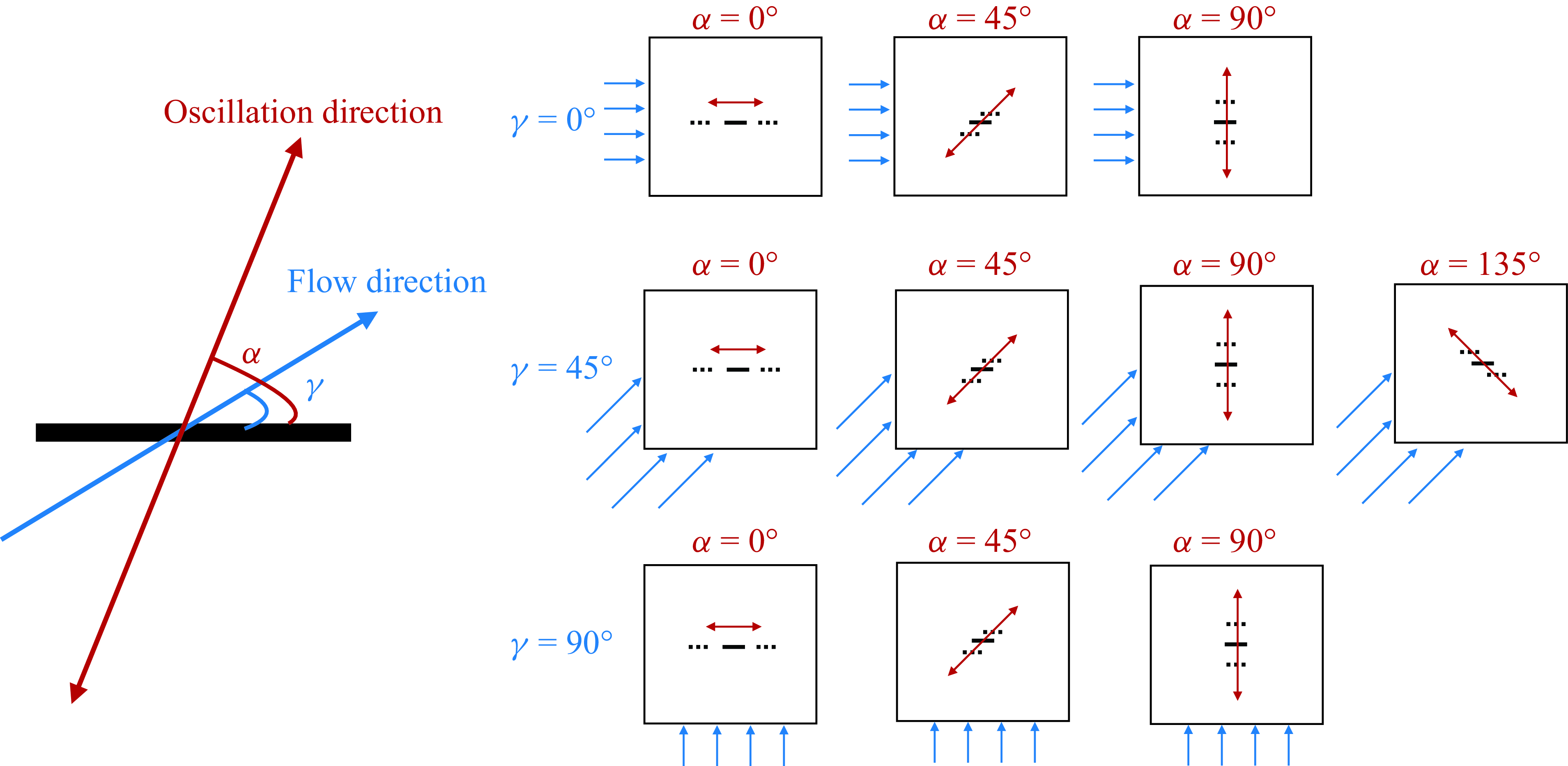
Figure 1. Schematic of the plate orientation and oscillation direction (angle $\alpha$
) and the background flow direction (angle
$\alpha$
) and the background flow direction (angle $\gamma$
).
$\gamma$
).
We also note that, in the present study, the Reynolds number based on the oncoming flow speed is 100, but the instantaneous Reynolds number based on the relative velocity between the oscillating plate and the flow can exceed 200 in some cases. Previous studies showed that the flow behind a plate is intrinsically three-dimensional (3-D) beyond a certain critical Reynolds number ( ${\approx}200$
behind a normal plate (Najjar & Vanka Reference Najjar and Vanka1995), and
${\approx}200$
behind a normal plate (Najjar & Vanka Reference Najjar and Vanka1995), and ${\approx}300$
behind an inclined plate (Yang et al. Reference Yang, Narasimhamurthy, Pettersen and Andersson2012)). Therefore, 3-D effects may begin at parameters near our values. However, Khaledi et al. (Reference Khaledi, Andersson, Barri and Pettersen2012) showed that, for a plate normal to the flow undergoing inline oscillations, the flow remains two-dimensional at
${\approx}300$
behind an inclined plate (Yang et al. Reference Yang, Narasimhamurthy, Pettersen and Andersson2012)). Therefore, 3-D effects may begin at parameters near our values. However, Khaledi et al. (Reference Khaledi, Andersson, Barri and Pettersen2012) showed that, for a plate normal to the flow undergoing inline oscillations, the flow remains two-dimensional at $Re_U=100$
if the oscillation frequency is sufficiently larger than the natural shedding frequency of the plate. (Two-dimensional flow was reported at plate-oscillation-to-natural-shedding-frequency ratios 1.74 and 2.1 for
$Re_U=100$
if the oscillation frequency is sufficiently larger than the natural shedding frequency of the plate. (Two-dimensional flow was reported at plate-oscillation-to-natural-shedding-frequency ratios 1.74 and 2.1 for $Re_U=100$
.) In the present study, the lowest oscillation frequency studied is at least twice the natural shedding frequency. Furthermore, the body oscillations seem to suppress the transition from two to three dimensions, at least for circular cylinders (Leontini, Thompson & Hourigan Reference Leontini, Thompson and Hourigan2007; Lo Jacono et al. Reference Jacono, David, Justin, Thompson and Sheridan2010). Therefore, we believe our 2-D formulation at
$Re_U=100$
.) In the present study, the lowest oscillation frequency studied is at least twice the natural shedding frequency. Furthermore, the body oscillations seem to suppress the transition from two to three dimensions, at least for circular cylinders (Leontini, Thompson & Hourigan Reference Leontini, Thompson and Hourigan2007; Lo Jacono et al. Reference Jacono, David, Justin, Thompson and Sheridan2010). Therefore, we believe our 2-D formulation at $Re_U=100$
is a reasonable model.
$Re_U=100$
is a reasonable model.
The structure of the paper is as follows. In § 2 we present the governing equations and numerical method. Section 3 presents the flow fields and the local heat transfer distributions in the benchmark cases of non-oscillating plates. Section 4 shows the effect of vorticity patterns on global and local heat transfer for oscillating plates with different orientations and oscillation directions. In § 5 we discuss the input power for this system, including the power to oscillate the plates and to drive the oncoming flow. Section 6 presents the conclusions.
2. Governing equations and numerical method
We consider a heated zero-thickness flat plate oscillating sinusoidally in a uniform oncoming flow at angle $\gamma$
relative to the plane of the plate (see figure 1). The plate oscillates in a direction with angle
$\gamma$
relative to the plane of the plate (see figure 1). The plate oscillates in a direction with angle $\alpha$
relative to the plane of the plate, different from
$\alpha$
relative to the plane of the plate, different from $\gamma$
in general. The problem is formulated in two dimensions. We non-dimensionalise all variables using the plate length
$\gamma$
in general. The problem is formulated in two dimensions. We non-dimensionalise all variables using the plate length $\ell ^\star$
as the characteristic length scale and the plate oscillation period
$\ell ^\star$
as the characteristic length scale and the plate oscillation period $1/f^\star$
as the characteristic time scale, with
$1/f^\star$
as the characteristic time scale, with $f^\star$
the plate oscillation frequency. The oscillation period is a convenient reference time scale for our computations, so that a fixed small time step is sufficient to resolve the dynamics over a period of oscillation. Then
$f^\star$
the plate oscillation frequency. The oscillation period is a convenient reference time scale for our computations, so that a fixed small time step is sufficient to resolve the dynamics over a period of oscillation. Then $f^\star \ell ^\star$
is the characteristic velocity scale. We use the fluid density
$f^\star \ell ^\star$
is the characteristic velocity scale. We use the fluid density $\rho _f^\star$
as the characteristic mass density.
$\rho _f^\star$
as the characteristic mass density.
We prescribe the plate’s oscillation velocity, $\boldsymbol{U}_b(t) = (U_b(t), V_b(t))$
as follows:
$\boldsymbol{U}_b(t) = (U_b(t), V_b(t))$
as follows:
 \begin{equation} (U_b,V_b) = \left (\frac {U_b^\star }{f^\star \ell ^\star },\frac {V_b^\star }{f^\star \ell ^\star }\right ) = 2 \pi A\sin (2\pi t)\left(1-e^{-(t/t_0)^2}\right) \left (\cos (\alpha ), \sin (\alpha )\right ), \end{equation}
where the starred variables and parameters are dimensional and the unstarred variables and parameters are dimensionless. The latter include $A$
, the plate’s oscillation amplitude (relative to its length). The exponential term makes the simulated flow start smoothly from rest. We use
$A$
, the plate’s oscillation amplitude (relative to its length). The exponential term makes the simulated flow start smoothly from rest. We use $t_0=0.2$
for all the simulations because it is small enough to make the exponential term decay quickly but large enough to ensure a smooth start.
$t_0=0.2$
for all the simulations because it is small enough to make the exponential term decay quickly but large enough to ensure a smooth start.
The governing equations for an incompressible viscous flow in the (non-inertial) frame of reference attached to the moving plate are (Li, Sherwin & Bearman Reference Li, Sherwin and Bearman2002; Alben Reference Alben2021a )
 \begin{align}& \frac {\partial \boldsymbol{u}}{\partial t} + \boldsymbol{u\cdot \nabla u} = -\boldsymbol{\nabla } p + \frac {1}{Re_f}\nabla ^2 \boldsymbol{u} - \frac {\textrm{d}\boldsymbol{U}_b}{\textrm{d}t}, \end{align}
 \begin{align}&\qquad\qquad\qquad \boldsymbol{\nabla \cdot u} = 0, \end{align}
with $\boldsymbol{u}(x, y, t)=(u(x, y, t), v(x, y, t))$
and
$\boldsymbol{u}(x, y, t)=(u(x, y, t), v(x, y, t))$
and $p(x, y, t)$
the flow velocity and pressure, respectively. Here,
$p(x, y, t)$
the flow velocity and pressure, respectively. Here, $Re_f$
is the frequency-based Reynolds number, included in the list of important dimensionless parameters for this problem
$Re_f$
is the frequency-based Reynolds number, included in the list of important dimensionless parameters for this problem
 \begin{equation} Re_f = \frac {f^\star {\ell ^\star }^2}{\nu ^\star }, \, \boldsymbol{U}_{\infty }=\frac {\boldsymbol{U}_{\infty }^\star }{f^\star \ell ^\star }, \, Re_U \!= \frac {|\boldsymbol{U}_{\infty }^\star |\ell ^\star }{\nu ^\star }=Re_f\times |\boldsymbol{U}_{\infty }| ,\, A = \frac {A^\star }{\ell ^\star }, \,\, \frac {A}{|\boldsymbol{U}_{\infty }|} =\frac {f^\star A^\star }{|\boldsymbol{U}_{\infty }^\star |_{_{_{\!}}}} . \end{equation}
Here, $\boldsymbol{U}_{\infty } = (U_{\infty }, V_{\infty }) = (|\boldsymbol{U}_{\infty }|\cos (\gamma ), |\boldsymbol{U}_{\infty }|\sin (\gamma ))$
is the steady far-field oncoming flow velocity and
$\boldsymbol{U}_{\infty } = (U_{\infty }, V_{\infty }) = (|\boldsymbol{U}_{\infty }|\cos (\gamma ), |\boldsymbol{U}_{\infty }|\sin (\gamma ))$
is the steady far-field oncoming flow velocity and $\nu^{\star}$
is the kinematic viscosity of the fluid. Besides the frequency-based Reynolds number
$\nu^{\star}$
is the kinematic viscosity of the fluid. Besides the frequency-based Reynolds number $Re_f$
, we can also define a Reynolds number based on
$Re_f$
, we can also define a Reynolds number based on $\boldsymbol{U}_{\infty }$
, which is
$\boldsymbol{U}_{\infty }$
, which is $Re_U$
in equation (2.3), also given by the product of
$Re_U$
in equation (2.3), also given by the product of $Re_f$
and
$Re_f$
and $|\boldsymbol{U}_{\infty }|$
. In this study, we vary both
$|\boldsymbol{U}_{\infty }|$
. In this study, we vary both $Re_f$
and
$Re_f$
and $\boldsymbol{U}_{\infty }$
but fix
$\boldsymbol{U}_{\infty }$
but fix $Re_U=100$
. The physical interpretation is that the plate length, fluid viscosity and background flow speed are considered fixed, but the plate oscillation frequency varies (as do the oscillation amplitude and direction, and the plate orientation). Another important parameter is
$Re_U=100$
. The physical interpretation is that the plate length, fluid viscosity and background flow speed are considered fixed, but the plate oscillation frequency varies (as do the oscillation amplitude and direction, and the plate orientation). Another important parameter is $A/|\boldsymbol{U}_{\infty }|$
, which we term the ‘oscillation velocity.’ It is proportional to the ratio between the plate’s oscillation velocity amplitude,
$A/|\boldsymbol{U}_{\infty }|$
, which we term the ‘oscillation velocity.’ It is proportional to the ratio between the plate’s oscillation velocity amplitude, $2\pi f^\star A^\star$
, and the oncoming flow velocity magnitude,
$2\pi f^\star A^\star$
, and the oncoming flow velocity magnitude, $|\boldsymbol{U}^\star _{\infty }|$
. For transverse oscillation (
$|\boldsymbol{U}^\star _{\infty }|$
. For transverse oscillation ( $\alpha = 90^\circ$
) in an in-plane flow (
$\alpha = 90^\circ$
) in an in-plane flow ( $\gamma = 0^\circ$
), the `plunge velocity’ (Rahman & Tafti Reference Rahman and Tafti2020a
) (defined as
$\gamma = 0^\circ$
), the `plunge velocity’ (Rahman & Tafti Reference Rahman and Tafti2020a
) (defined as $\pi f^\star A^\star /|\boldsymbol{U}_{\infty }^\star | = \pi A/|\boldsymbol{U}_{\infty }|$
), or `Strouhal number’ (twice the oscillation velocity) (Triantafyllou et al. Reference Triantafyllou, Triantafyllou and Gopalkrishnan1991, Reference Triantafyllou, Triantafyllou and Grosenbaugh1993) are often used, particularly in studies of locomotion and fluid–structure interaction. Because we consider a wide range of oscillation and flow directions, we use ‘oscillation velocity’ for this class of motions. Rahman & Tafti (Reference Rahman and Tafti2020a
) found that the rate of heat transfer is increased at higher
$\pi f^\star A^\star /|\boldsymbol{U}_{\infty }^\star | = \pi A/|\boldsymbol{U}_{\infty }|$
), or `Strouhal number’ (twice the oscillation velocity) (Triantafyllou et al. Reference Triantafyllou, Triantafyllou and Gopalkrishnan1991, Reference Triantafyllou, Triantafyllou and Grosenbaugh1993) are often used, particularly in studies of locomotion and fluid–structure interaction. Because we consider a wide range of oscillation and flow directions, we use ‘oscillation velocity’ for this class of motions. Rahman & Tafti (Reference Rahman and Tafti2020a
) found that the rate of heat transfer is increased at higher $A/|\boldsymbol{U}_{\infty }|$
. However, the flow also becomes very chaotic at high
$A/|\boldsymbol{U}_{\infty }|$
. However, the flow also becomes very chaotic at high $A/|\boldsymbol{U}_{\infty }|$
. In this study, we mainly study flows with
$A/|\boldsymbol{U}_{\infty }|$
. In this study, we mainly study flows with $A/|\boldsymbol{U}_{\infty }|=0.2$
and
$A/|\boldsymbol{U}_{\infty }|=0.2$
and $0.3$
. At these relatively low
$0.3$
. At these relatively low $A/|\boldsymbol{U}_{\infty }|$
values (compared with the range studied by Rahman & Tafti (Reference Rahman and Tafti2020a
)), the flow is typically tractable and heat transfer enhancement is significant so that we can obtain insight into how oscillatory motions alter global and local heat transfer.
$A/|\boldsymbol{U}_{\infty }|$
values (compared with the range studied by Rahman & Tafti (Reference Rahman and Tafti2020a
)), the flow is typically tractable and heat transfer enhancement is significant so that we can obtain insight into how oscillatory motions alter global and local heat transfer.
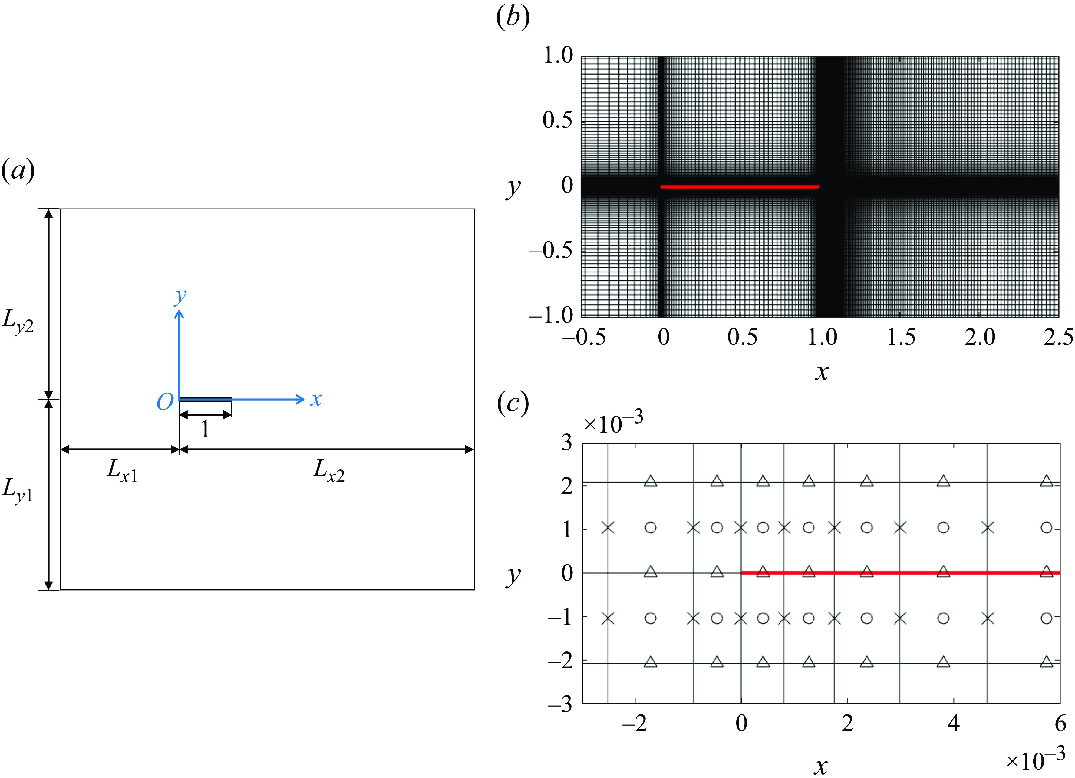
Figure 2. (a) Schematic of the computational domain. All the parameters shown are dimensionless. (b) Example of the non-uniform grid near the plate (red). (c) The marker-and-cell grid near the left edge of the plate. The flow velocity components $u$
and
$u$
and $v$
are solved at the crosses and triangles, respectively, while the pressure
$v$
are solved at the crosses and triangles, respectively, while the pressure $p$
and temperature
$p$
and temperature $T$
are solved at the circles.
$T$
are solved at the circles.
The temperature field $T(x,y,t)$
is governed by the unsteady advection-diffusion equation
$T(x,y,t)$
is governed by the unsteady advection-diffusion equation
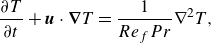 \begin{equation} \frac {\partial T}{\partial t} + \boldsymbol{u}\cdot \boldsymbol{\nabla }T = \frac {1}{Re_f Pr}\nabla ^2 T, \end{equation}
where $Pr = \nu ^\star /\kappa ^\star$
is the Prandtl number, with
$Pr = \nu ^\star /\kappa ^\star$
is the Prandtl number, with $\kappa ^\star$
the thermal diffusivity. In this study, we take air as the fluid, with
$\kappa ^\star$
the thermal diffusivity. In this study, we take air as the fluid, with $Pr=0.7$
. As shown in figure 2(a), the heated plate is positioned at
$Pr=0.7$
. As shown in figure 2(a), the heated plate is positioned at $0\leqslant x \leqslant 1, y=0$
. For the temperature boundary conditions on the plate, we consider two cases
$0\leqslant x \leqslant 1, y=0$
. For the temperature boundary conditions on the plate, we consider two cases
 \begin{align} &\qquad\qquad\quad{\text {Fixed temperature:}} \,\, T|_{y=0^+} = T|_{y=0^-} = 1 \,\, \text{for}\ 0\leqslant x \leqslant 1. \end{align}
 \begin{align}& {\text {Fixed heat flux:}} \,\, -\left .\frac {\partial T}{\partial y}\right |_{y=0^+}+\left .\frac {\partial T}{\partial y}\right |_{y=0^-} = 2, \,\, T|_{y=0^+} = T|_{y=0^-}, \quad \text{for}\ 0\leqslant x \leqslant 1. \end{align}
In (2.5) the plate temperature is fixed, while in (2.6) the heat flux per unit plate length is fixed. In the latter case we have also equated the temperatures of the top and bottom surfaces of the plate, as we assume the plate is a thin conducting material. If instead of (2.6) we used $-\partial _y T(y=0^+) = \partial _y T(y=0^-) = 1$
, the top and bottom surfaces of the plate would have different temperatures in general.
$-\partial _y T(y=0^+) = \partial _y T(y=0^-) = 1$
, the top and bottom surfaces of the plate would have different temperatures in general.
We solve equation (2.2) as a fully coupled system for $\boldsymbol{u}$
and
$\boldsymbol{u}$
and $p$
, using essentially the same method as in Alben (Reference Alben2021a
), a second-order finite-difference method on the MAC (marker-and-cell) grid (Harlow & Welch Reference Harlow and Welch1965). A portion of the MAC grid is shown in figure 2(c). We solve
$p$
, using essentially the same method as in Alben (Reference Alben2021a
), a second-order finite-difference method on the MAC (marker-and-cell) grid (Harlow & Welch Reference Harlow and Welch1965). A portion of the MAC grid is shown in figure 2(c). We solve $u$
at the crosses,
$u$
at the crosses, $v$
at the triangles and
$v$
at the triangles and $p$
at the circles. The grid spacing is larger toward the boundary of the computational domain and smaller near the plate, where the vorticity is large. An example of the grid is shown in figure 2(b). The details for generating the non-uniform mesh are given in Appendix A. The distances from the plate to the outer boundary (given by
$p$
at the circles. The grid spacing is larger toward the boundary of the computational domain and smaller near the plate, where the vorticity is large. An example of the grid is shown in figure 2(b). The details for generating the non-uniform mesh are given in Appendix A. The distances from the plate to the outer boundary (given by $L_{x1}$
,
$L_{x1}$
, $L_{x2}$
,
$L_{x2}$
, $L_{y1}$
,
$L_{y1}$
, $L_{y2}$
in figure 2(a) and the outer boundary conditions are chosen differently for each value of
$L_{y2}$
in figure 2(a) and the outer boundary conditions are chosen differently for each value of $\gamma$
to limit the influence of the outer boundary. We use Dirichlet boundary conditions at the inflow sides and Neumann boundary conditions at the outflow sides. For sides parallel to the mean oncoming flow, we set the normal velocity to the far-field value, and impose zero shear, to avoid vorticity generation (Tamaddon-Jahromi, Townsend & Webster Reference Tamaddon-Jahromi, Townsend and Webster1994; Sen, Mittal & Biswas Reference Sen, Mittal and Biswas2009). These boundary conditions are listed in table 1. On the plate surface, we apply no-slip boundary conditions. At
$\gamma$
to limit the influence of the outer boundary. We use Dirichlet boundary conditions at the inflow sides and Neumann boundary conditions at the outflow sides. For sides parallel to the mean oncoming flow, we set the normal velocity to the far-field value, and impose zero shear, to avoid vorticity generation (Tamaddon-Jahromi, Townsend & Webster Reference Tamaddon-Jahromi, Townsend and Webster1994; Sen, Mittal & Biswas Reference Sen, Mittal and Biswas2009). These boundary conditions are listed in table 1. On the plate surface, we apply no-slip boundary conditions. At $t=0$
, we assume steady uniform flow with
$t=0$
, we assume steady uniform flow with $\boldsymbol{u}(x,y,0) = \boldsymbol{U}_{\infty }$
(at points off of the plate), except in one case,
$\boldsymbol{u}(x,y,0) = \boldsymbol{U}_{\infty }$
(at points off of the plate), except in one case, $\alpha = \gamma = 90^\circ$
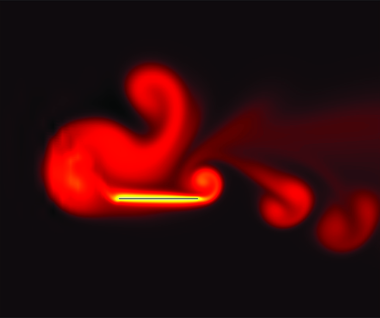
, where we use an asymmetric initial flow described in § 4.2.3. In figure 3 we provide examples of typical vorticity fields, with
$\alpha = \gamma = 90^\circ$
, where we use an asymmetric initial flow described in § 4.2.3. In figure 3 we provide examples of typical vorticity fields, with $\gamma$
increasing from the top row to the bottom row, and
$\gamma$
increasing from the top row to the bottom row, and $\alpha$
increasing from left to right within each row. The overall orientation of the wake relative to the body is set by
$\alpha$
increasing from left to right within each row. The overall orientation of the wake relative to the body is set by $\gamma$
; both
$\gamma$
; both $\gamma$
and
$\gamma$
and $\alpha$
affect the vorticity patterns around the body and particularly within the wake. A main focus of the current study is the effect of these vorticity patterns on heat transfer.
$\alpha$
affect the vorticity patterns around the body and particularly within the wake. A main focus of the current study is the effect of these vorticity patterns on heat transfer.
Table 1. The dimensions of the computational domain, the number of grid cells along $x$
and
$x$
and $y$
(denoted
$y$
(denoted $m$
and
$m$
and $n$
, respectively) and the boundary conditions, with
$n$
, respectively) and the boundary conditions, with $a_1 = (1+\textrm{sign}(-V_b))/2$
,
$a_1 = (1+\textrm{sign}(-V_b))/2$
, $a_2 = (1-\textrm{sign}(-V_b))/2$
,
$a_2 = (1-\textrm{sign}(-V_b))/2$
, $b_1 = (1+\textrm{sign}(-U_b))/2$
and
$b_1 = (1+\textrm{sign}(-U_b))/2$
and $b_2 = (1-\textrm{sign}(-U_b))/2$
.
$b_2 = (1-\textrm{sign}(-U_b))/2$
.
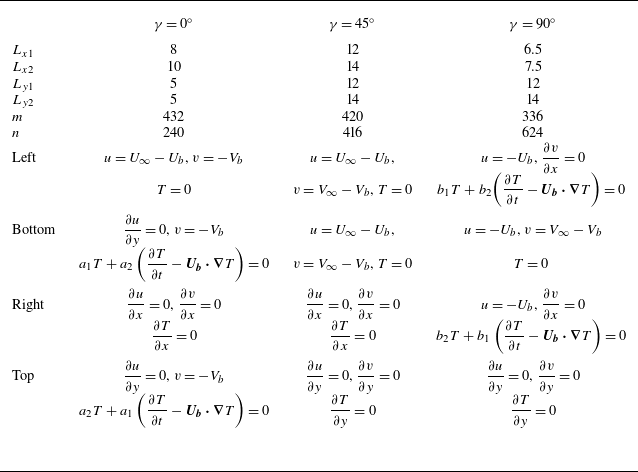
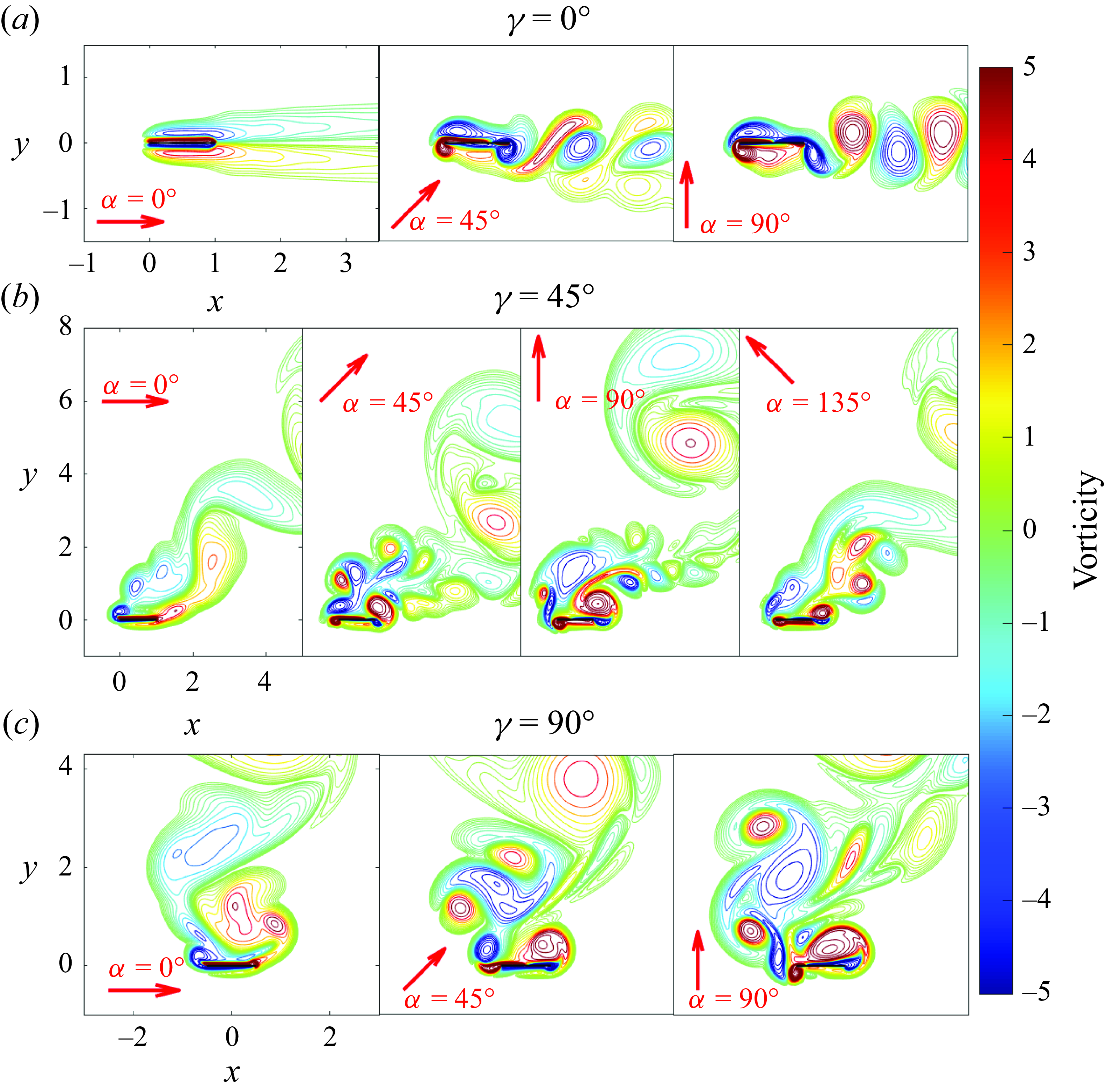
Figure 3. Examples of the vorticity fields for different plate orientations and oscillation directions. The rows from top to bottom have (a) $\gamma = 0^\circ$
, (b)
$\gamma = 0^\circ$
, (b) $45^\circ$
and (c)
$45^\circ$
and (c) $90^\circ$
. The red arrow indicates instantaneous plate oscillation direction given by
$90^\circ$
. The red arrow indicates instantaneous plate oscillation direction given by $\alpha$
. Within each row,
$\alpha$
. Within each row, $\alpha$
increases in increments of
$\alpha$
increases in increments of $45^\circ$
moving rightward, starting at
$45^\circ$
moving rightward, starting at $0^\circ$
in the leftmost panel. All of the examples have
$0^\circ$
in the leftmost panel. All of the examples have $Re_f=100$
,
$Re_f=100$
, $Re_U=100$
,
$Re_U=100$
, $A=0.2$
and
$A=0.2$
and $A/|\boldsymbol{U}_{\infty }|=0.2$
.
$A/|\boldsymbol{U}_{\infty }|=0.2$
.
After computing the flow velocity $\boldsymbol{u}$
, we solve for the temperature using a second-order discretisation of (2.4) at the same grid points as
$\boldsymbol{u}$
, we solve for the temperature using a second-order discretisation of (2.4) at the same grid points as $p$
(the centres of the MAC grid cells). Either (2.5) or (2.6) is applied in one-sided finite-difference formulas for the
$p$
(the centres of the MAC grid cells). Either (2.5) or (2.6) is applied in one-sided finite-difference formulas for the $y$
-derivatives in (2.4) on either side of the plate, depending on whether we fix the plate temperature or the heat flux. As with
$y$
-derivatives in (2.4) on either side of the plate, depending on whether we fix the plate temperature or the heat flux. As with $\boldsymbol{u}$
, we apply different outer boundary conditions for
$\boldsymbol{u}$
, we apply different outer boundary conditions for $T$
depending on
$T$
depending on $\gamma$
, i.e. which sides of the computational domain are the inflow and outflow boundaries. These are listed in table 1. We apply
$\gamma$
, i.e. which sides of the computational domain are the inflow and outflow boundaries. These are listed in table 1. We apply $T=0$
at inflow boundaries and
$T=0$
at inflow boundaries and $\partial T/\partial n = 0$
at outflow boundaries, with
$\partial T/\partial n = 0$
at outflow boundaries, with $\partial /\partial n$
the normal derivative. For sides parallel to the mean oncoming flow, we switch between Dirichlet and outflow boundary conditions for
$\partial /\partial n$
the normal derivative. For sides parallel to the mean oncoming flow, we switch between Dirichlet and outflow boundary conditions for $T$
depending on whether the flow is inward or outward at a given time, as shown in table 1. At
$T$
depending on whether the flow is inward or outward at a given time, as shown in table 1. At $t = 0$
the temperature is set to zero at all points in the fluid, i.e.
$t = 0$
the temperature is set to zero at all points in the fluid, i.e. $T(x,y,0)=0$
. A comparison of results with different domain and mesh sizes is given in Appendix B. Validations of our numerical method against previous theoretical and computational results are provided in Appendix C.
$T(x,y,0)=0$
. A comparison of results with different domain and mesh sizes is given in Appendix B. Validations of our numerical method against previous theoretical and computational results are provided in Appendix C.
The main heat transfer performance metric in this study is the Nusselt number, the local heat flux relative to the difference between the plate temperature $T_{{plate}}$
and the far-field fluid temperature
$T_{{plate}}$
and the far-field fluid temperature $T_\infty$
, set to zero here (Incropera et al. Reference Incropera, DeWitt, Bergman and Lavine2006)
$T_\infty$
, set to zero here (Incropera et al. Reference Incropera, DeWitt, Bergman and Lavine2006)
 \begin{align} Nu = \frac {\partial T/\partial y}{T_{{plate}} - T_\infty }. \end{align}
A larger rate of heat transfer corresponds to larger $Nu$
. With the fixed-plate-temperature boundary condition, the denominator of (2.7) is fixed at unity while the numerator varies along the plate. We consider two local and one global Nusselt number in this case
$Nu$
. With the fixed-plate-temperature boundary condition, the denominator of (2.7) is fixed at unity while the numerator varies along the plate. We consider two local and one global Nusselt number in this case
 \begin{align} &Nu_{{top}}(x, t) = -\left .\frac {\partial T}{\partial y}\right |_{y=0^+}, \quad Nu_{{bot}}(x,t) = \left .\frac {\partial T}{\partial y}\right |_{y=0^-},\nonumber\\& \qquad \overline {Nu}(t) = \displaystyle \int _0^1 -\left .\frac {\partial T}{\partial y}\right |_{y=0^+} + \left .\frac {\partial T}{\partial y}\right |_{y=0^-}\, \textrm{d}x. \end{align}
The first two Nusselt numbers are the local heat fluxes from the plate’s top and bottom surfaces, respectively, while the third is the global Nusselt number, the total heat flux from both plate surfaces.
With the fixed-heat-flux boundary condition, the numerator of (2.7) summed over both sides of the plate is fixed at each $x$
while
$x$
while $T_{{plate}}$
in the denominator varies with
$T_{{plate}}$
in the denominator varies with $x$
. In this case
$x$
. In this case $Nu$
is inversely proportional to
$Nu$
is inversely proportional to $T_{{plate}}$
, so lower plate temperature corresponds to better heat transfer performance. In this case, instead of
$T_{{plate}}$
, so lower plate temperature corresponds to better heat transfer performance. In this case, instead of $Nu$
, we use the plate-temperature distribution
$Nu$
, we use the plate-temperature distribution $T_{{plate}}(x, t)$
, the maximum plate temperature
$T_{{plate}}(x, t)$
, the maximum plate temperature $T_{max }(t)$
and the spatially averaged plate temperature
$T_{max }(t)$
and the spatially averaged plate temperature $T_{{avg}}(t)$
as performance metrics
$T_{{avg}}(t)$
as performance metrics
 \begin{equation} T_{{plate}}(x, t) = T|_{y=0}, \quad T_{max }(t) = \max (T_{{plate}}), \quad T_{{avg}}(t) = \displaystyle \int _0^1 T_{{plate}}(x, t)\, \textrm{d}x. \end{equation}
In the following sections, we will also examine the time averages of quantities in equations (2.8) and (2.9), denoted as $\langle \cdot \rangle$
. In § 4.1 we explain how we choose appropriate time spans for the time averages.
$\langle \cdot \rangle$
. In § 4.1 we explain how we choose appropriate time spans for the time averages.
3. Non-oscillating plate in steady oncoming flows
In figures 4 and 5, we show results for a non-oscillating plate in steady oncoming flows, which can be taken as a reference state for investigating how plate oscillations influence heat transfer. As in the cases with oscillating plates, the Reynolds number of the oncoming flow is fixed at $Re_U=100$
for different plate orientations. However, since the plate is not oscillating,
$Re_U=100$
for different plate orientations. However, since the plate is not oscillating, $t$
is non-dimensionalised using
$t$
is non-dimensionalised using $\ell ^\star /|\boldsymbol{U}^\star _{\infty }|$
instead of
$\ell ^\star /|\boldsymbol{U}^\star _{\infty }|$
instead of $1/f^\star$
.
$1/f^\star$
.
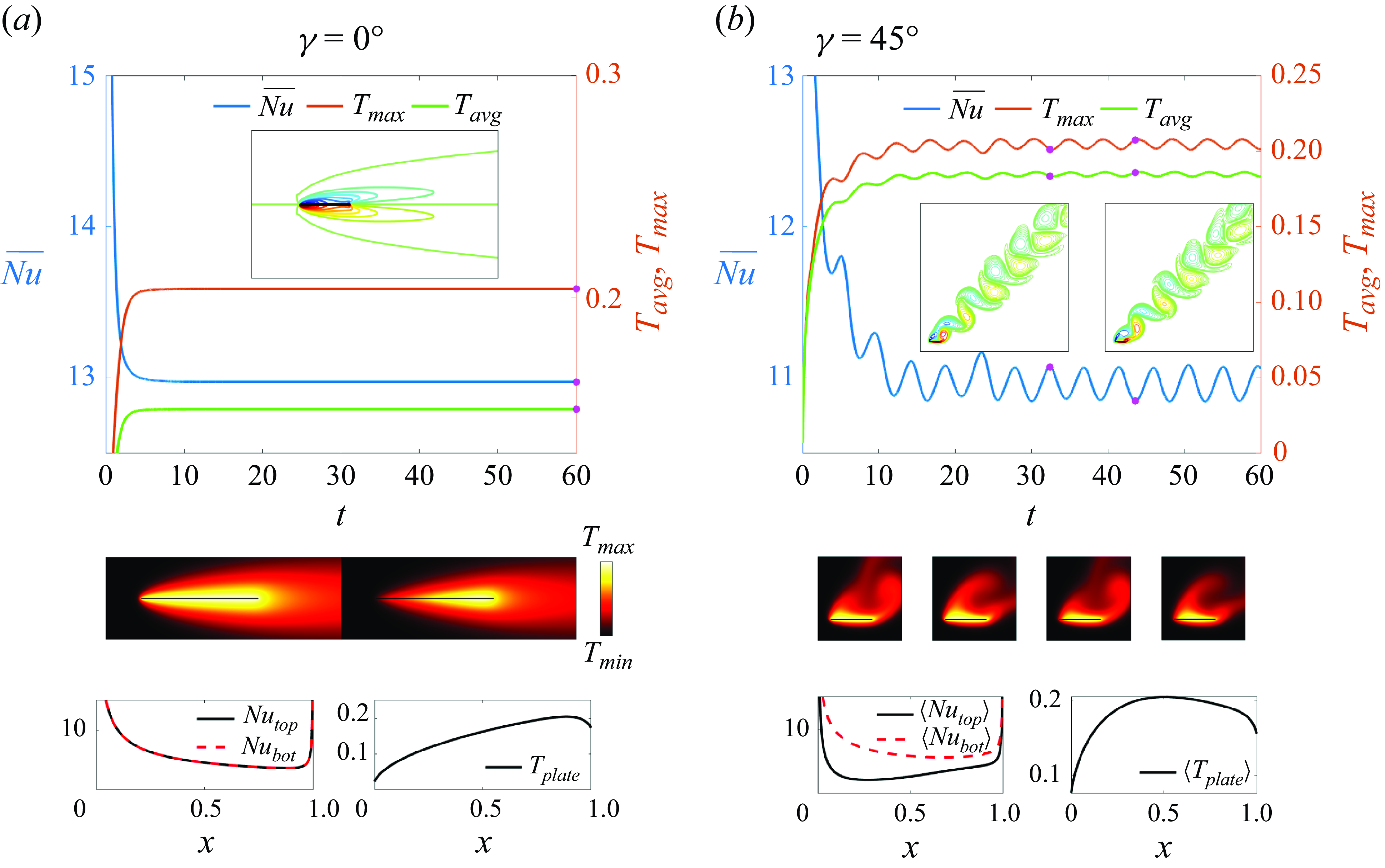
Figure 4. Heat transfer from a non-oscillating plate in steady oncoming flows angled at $\gamma = 0^\circ$
(panel (a)), and
$\gamma = 0^\circ$
(panel (a)), and $\gamma = 45^\circ$
(panel (b)). The time series of
$\gamma = 45^\circ$
(panel (b)). The time series of $\overline {Nu}$
,
$\overline {Nu}$
, $T_{max }$
and
$T_{max }$
and $T_{{avg}}$
with selected snapshots of the vorticity field and temperature field (at times marked with pink dots) are shown for each case. In panel (a), the temperature field snapshots show the isothermal-plate and fixed-flux cases on the left and right, respectively. In panel (b) the same quantities are shown but with four temperature snapshots, the leftmost two for the isothermal-plate case, and the rightmost two for the fixed-flux case. At the bottom of each panel, the local
$T_{{avg}}$
with selected snapshots of the vorticity field and temperature field (at times marked with pink dots) are shown for each case. In panel (a), the temperature field snapshots show the isothermal-plate and fixed-flux cases on the left and right, respectively. In panel (b) the same quantities are shown but with four temperature snapshots, the leftmost two for the isothermal-plate case, and the rightmost two for the fixed-flux case. At the bottom of each panel, the local $Nu$
and plate temperatures are shown, steady in panel (a) and averaged over the last four periods in panel (b).
$Nu$
and plate temperatures are shown, steady in panel (a) and averaged over the last four periods in panel (b).
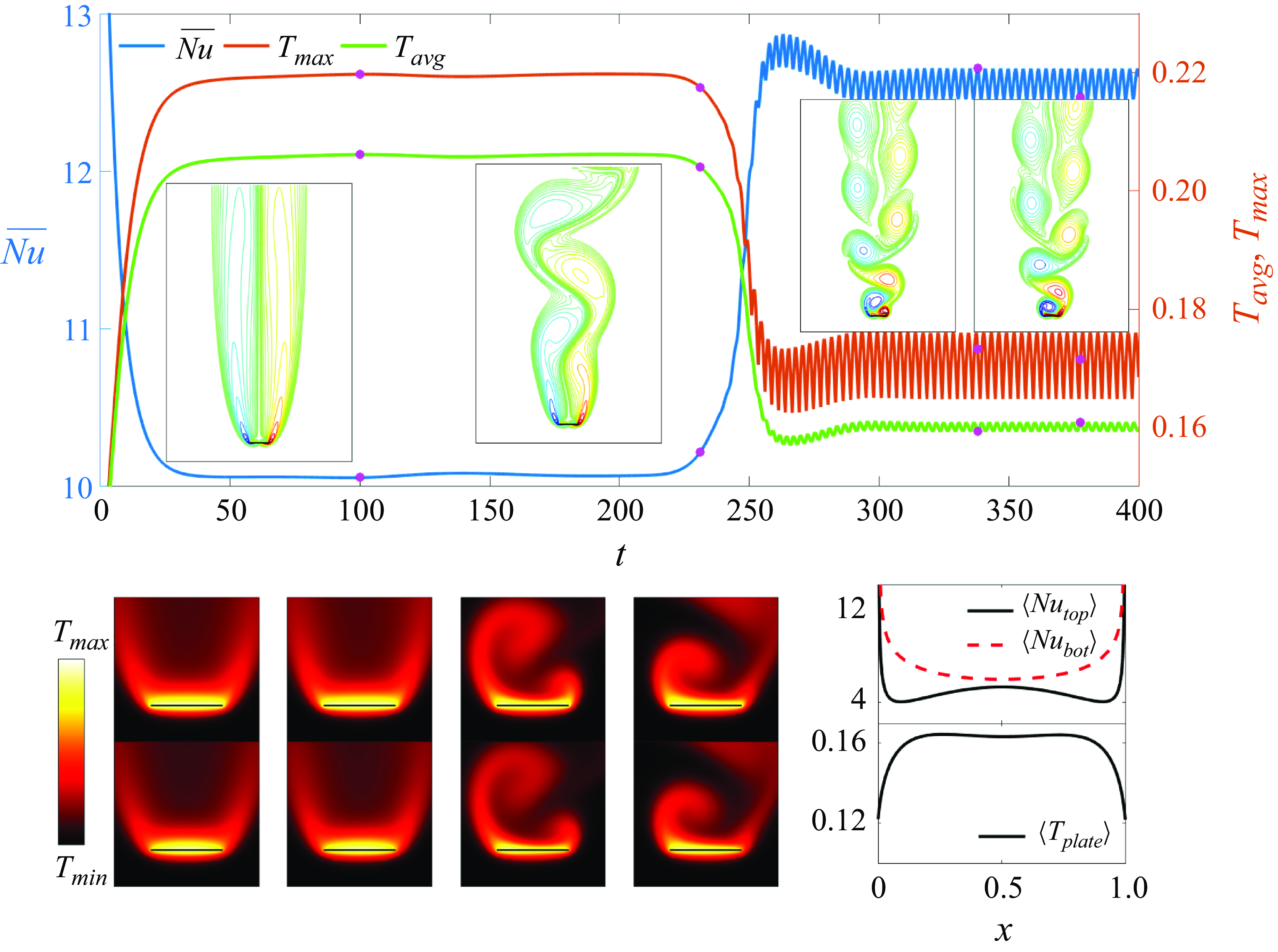
Figure 5. Heat transfer from a non-oscillating plate in a steady oncoming flow angled at $\gamma = 90^\circ$
. The time series of
$\gamma = 90^\circ$
. The time series of $\overline {Nu}$
,
$\overline {Nu}$
, $T_{max }$
and
$T_{max }$
and $T_{{avg}}$
with selected snapshots of the vorticity field and temperature field (at times marked with pink dots) are shown at the bottom left. The first row of the temperature snapshots is for the isothermal case and the second row is for the fixed-flux case. The local
$T_{{avg}}$
with selected snapshots of the vorticity field and temperature field (at times marked with pink dots) are shown at the bottom left. The first row of the temperature snapshots is for the isothermal case and the second row is for the fixed-flux case. The local $Nu$
and plate temperature, averaged over the last four periods, are shown at the bottom right.
$Nu$
and plate temperature, averaged over the last four periods, are shown at the bottom right.
In figure 4(a) the plate is aligned with the flow ( $\gamma =0^\circ$
). We have rapid convergence to a steady flow with symmetrical boundary layers along both sides of the plate. The temperature field is also up–down symmetric, and the thickness of the thermal boundary layer increases toward the trailing edge (the right edge). For the isothermal plate (left sides of the bottom rows of panel (a)), the local Nusselt number is equal on the top and bottom surfaces, and larger near the leading edge than the trailing edge. Previous computations show that the local Nusselt number diverges at both edges (Dennis & Smith Reference Dennis and Smith1966; Rahman & Tafti Reference Rahman and Tafti2020a
). When instead the heat flux from the plate is fixed (right sides of the bottom rows of panel (a)), the hottest spot is located slightly upstream of the trailing edge.
$\gamma =0^\circ$
). We have rapid convergence to a steady flow with symmetrical boundary layers along both sides of the plate. The temperature field is also up–down symmetric, and the thickness of the thermal boundary layer increases toward the trailing edge (the right edge). For the isothermal plate (left sides of the bottom rows of panel (a)), the local Nusselt number is equal on the top and bottom surfaces, and larger near the leading edge than the trailing edge. Previous computations show that the local Nusselt number diverges at both edges (Dennis & Smith Reference Dennis and Smith1966; Rahman & Tafti Reference Rahman and Tafti2020a
). When instead the heat flux from the plate is fixed (right sides of the bottom rows of panel (a)), the hottest spot is located slightly upstream of the trailing edge.
In figure 4(b), with an oblique oncoming flow relative to the plate ( $\gamma =45^\circ$
), we observe a periodic flow with a von Kármán vortex street wake instead of the steady flow at
$\gamma =45^\circ$
), we observe a periodic flow with a von Kármán vortex street wake instead of the steady flow at $\gamma =0^\circ$
. During one complete period, a negative vortex (in blue) and a positive vortex (in red) form and shed at the left and right edges of the top wall alternately. Because the flow is oblique, the negative vortex covers a larger portion of the top wall, shown in the rightmost vorticity snapshot in panel (b). The rotation of the negative vortex sweeps hot fluid along the top surface from the right edge toward the left edge, which makes the thermal boundary layer thicker near the left edge. Therefore, the time-averaged local Nusselt number of the top wall
$\gamma =0^\circ$
. During one complete period, a negative vortex (in blue) and a positive vortex (in red) form and shed at the left and right edges of the top wall alternately. Because the flow is oblique, the negative vortex covers a larger portion of the top wall, shown in the rightmost vorticity snapshot in panel (b). The rotation of the negative vortex sweeps hot fluid along the top surface from the right edge toward the left edge, which makes the thermal boundary layer thicker near the left edge. Therefore, the time-averaged local Nusselt number of the top wall $\langle Nu_{{top}} \rangle$
(black solid line), which is roughly the inverse of the temperature boundary layer thickness, has a minimum near the left edge. There are no vortices adjacent to the bottom wall, and the thermal boundary layer thickness is more uniform along the bottom wall. The thermal boundary layer is much thinner along the bottom wall, so
$\langle Nu_{{top}} \rangle$
(black solid line), which is roughly the inverse of the temperature boundary layer thickness, has a minimum near the left edge. There are no vortices adjacent to the bottom wall, and the thermal boundary layer thickness is more uniform along the bottom wall. The thermal boundary layer is much thinner along the bottom wall, so $\langle Nu_{{bot}} \rangle \gt \langle Nu_{{top}} \rangle$
. The temperature fields in the case of fixed heat flux from the plate (two rightmost snapshots) are qualitatively similar to those for the isothermal plate (two leftmost snapshots). The time-averaged plate temperature
$\langle Nu_{{bot}} \rangle \gt \langle Nu_{{top}} \rangle$
. The temperature fields in the case of fixed heat flux from the plate (two rightmost snapshots) are qualitatively similar to those for the isothermal plate (two leftmost snapshots). The time-averaged plate temperature $\langle T_{{plate}} \rangle$
rises sharply from the left edge to a maximum near the centre, and decreases more gradually on the right side.
$\langle T_{{plate}} \rangle$
rises sharply from the left edge to a maximum near the centre, and decreases more gradually on the right side.
For the vertical oncoming flow ( $\gamma =90^\circ$
) in figure 5, the vortex wake instead has a long transition from a symmetric initial state to the time-periodic alternating-vortex-shedding state. Initially, there is a pair of recirculation bubbles behind the plate, and the corresponding temperature field is symmetric about the middle of the plate, as shown in the first column of the temperature snapshots. The thermal boundary layer thickness is fairly uniform and thinner along the bottom wall, as before. Small asymmetric perturbations (from numerical round-off error) grow exponentially during this time and reach O(1) amplitude at
$\gamma =90^\circ$
) in figure 5, the vortex wake instead has a long transition from a symmetric initial state to the time-periodic alternating-vortex-shedding state. Initially, there is a pair of recirculation bubbles behind the plate, and the corresponding temperature field is symmetric about the middle of the plate, as shown in the first column of the temperature snapshots. The thermal boundary layer thickness is fairly uniform and thinner along the bottom wall, as before. Small asymmetric perturbations (from numerical round-off error) grow exponentially during this time and reach O(1) amplitude at $t \approx 200$
. During this instability, which has been studied more extensively for circular cylinders than for flat plates (Thompson et al. Reference Thompson, Radi, Rao, Sheridan and Hourigan2014), the long recirculation bubbles become wavy and shed vortices, as shown in the second vorticity field snapshot. However, the corresponding temperature field close to the plate does not change much from the first stage, as shown in the second column of the temperature snapshots, because the flow is still fairly symmetric close to the plate. At
$t \approx 200$
. During this instability, which has been studied more extensively for circular cylinders than for flat plates (Thompson et al. Reference Thompson, Radi, Rao, Sheridan and Hourigan2014), the long recirculation bubbles become wavy and shed vortices, as shown in the second vorticity field snapshot. However, the corresponding temperature field close to the plate does not change much from the first stage, as shown in the second column of the temperature snapshots, because the flow is still fairly symmetric close to the plate. At $t \approx 300$
, the system reaches a periodic state, with alternating shedding of positive and negative vortices from the edges, giving rise to a von Kármán vortex street. The near-wake flow and temperature fields (third and the fourth columns of the temperature snapshots) are now very asymmetric. The top panel shows jumps in the global Nusselt number
$t \approx 300$
, the system reaches a periodic state, with alternating shedding of positive and negative vortices from the edges, giving rise to a von Kármán vortex street. The near-wake flow and temperature fields (third and the fourth columns of the temperature snapshots) are now very asymmetric. The top panel shows jumps in the global Nusselt number $\overline {Nu}$
,
$\overline {Nu}$
, $T_{{avg}}$
and
$T_{{avg}}$
and $T_{max }$
during the transition at
$T_{max }$
during the transition at $t \approx 250$
. Similarly to the case of
$t \approx 250$
. Similarly to the case of $\gamma =45^\circ$
, the vortices behind the plate make the thermal boundary layer thinner along the top wall, increasing heat transfer, although
$\gamma =45^\circ$
, the vortices behind the plate make the thermal boundary layer thinner along the top wall, increasing heat transfer, although $\langle Nu_{{bot}} \rangle$
is still larger than
$\langle Nu_{{bot}} \rangle$
is still larger than $\langle Nu_{{top}} \rangle$
. The plots of
$\langle Nu_{{top}} \rangle$
. The plots of $\langle Nu_{{top}} \rangle$
,
$\langle Nu_{{top}} \rangle$
, $\langle Nu_{{bot}} \rangle$
and
$\langle Nu_{{bot}} \rangle$
and $\langle T_{{plate}} \rangle$
are symmetric about the plate centre when
$\langle T_{{plate}} \rangle$
are symmetric about the plate centre when $\gamma =90^\circ$
, reflecting the symmetry of the plate with respect to the oncoming flow. The vortices at the two edges take the same time to develop and have the same strength. The vortices alternately sweep hot fluid toward the two edges, so the thermal boundary layer is thinnest in the middle of the plate, where
$\gamma =90^\circ$
, reflecting the symmetry of the plate with respect to the oncoming flow. The vortices at the two edges take the same time to develop and have the same strength. The vortices alternately sweep hot fluid toward the two edges, so the thermal boundary layer is thinnest in the middle of the plate, where $\langle Nu_{{top}} \rangle$
has a local maximum and
$\langle Nu_{{top}} \rangle$
has a local maximum and $\langle T_{{plate}} \rangle$
has a local minimum. Thompson et al. (Reference Thompson, Radi, Rao, Sheridan and Hourigan2014) studied the transient wake development for elliptical cylinders ranging from a flat plate to a circular cylinder at a Reynolds number of
$\langle T_{{plate}} \rangle$
has a local minimum. Thompson et al. (Reference Thompson, Radi, Rao, Sheridan and Hourigan2014) studied the transient wake development for elliptical cylinders ranging from a flat plate to a circular cylinder at a Reynolds number of $150$
. Using a much larger domain than we use here, they reported not only the von Kármán street behind the plate but also secondary vortex shedding further downstream. We believe that the secondary vortex shedding has negligible influence on heat transfer as the near wake reported by Thompson et al. (Reference Thompson, Radi, Rao, Sheridan and Hourigan2014) is very similar to what we show in figure 5 and very close to periodic, despite the existence of the secondary vortex shedding.
$150$
. Using a much larger domain than we use here, they reported not only the von Kármán street behind the plate but also secondary vortex shedding further downstream. We believe that the secondary vortex shedding has negligible influence on heat transfer as the near wake reported by Thompson et al. (Reference Thompson, Radi, Rao, Sheridan and Hourigan2014) is very similar to what we show in figure 5 and very close to periodic, despite the existence of the secondary vortex shedding.
Our discussion so far has shown that the local heat transfer is quite different for $\gamma =0^\circ , 45^\circ$
and
$\gamma =0^\circ , 45^\circ$
and $90^\circ$
. The time-averaged global heat transfer quantities
$90^\circ$
. The time-averaged global heat transfer quantities $\langle \overline {Nu} \rangle$
and
$\langle \overline {Nu} \rangle$
and $\langle T_{{avg}} \rangle$
can be inferred from the graphs in figures 4 and 5 at the latest times (in the final periodic steady state for
$\langle T_{{avg}} \rangle$
can be inferred from the graphs in figures 4 and 5 at the latest times (in the final periodic steady state for $\gamma =90^\circ$
, after the symmetry breaking). For the isothermal plate,
$\gamma =90^\circ$
, after the symmetry breaking). For the isothermal plate, $\gamma =0^\circ$
has the best heat transfer i.e. the largest
$\gamma =0^\circ$
has the best heat transfer i.e. the largest $\langle \overline {Nu} \rangle$
, 13.0, and the smallest
$\langle \overline {Nu} \rangle$
, 13.0, and the smallest $\langle T_{{avg}} \rangle$
, 0.15. Slightly worse is
$\langle T_{{avg}} \rangle$
, 0.15. Slightly worse is $\gamma =90^\circ$
, with
$\gamma =90^\circ$
, with $\langle \overline {Nu} \rangle = 12.6$
and
$\langle \overline {Nu} \rangle = 12.6$
and $\langle T_{{avg}} \rangle =0.16$
. Third best is
$\langle T_{{avg}} \rangle =0.16$
. Third best is $\gamma =45^\circ$
with
$\gamma =45^\circ$
with $\langle \overline {Nu} \rangle = 11.0$
and
$\langle \overline {Nu} \rangle = 11.0$
and $\langle T_{{avg}} \rangle =0.19$
. At
$\langle T_{{avg}} \rangle =0.19$
. At $\gamma =45^\circ$
, local heat transfer is decreased particularly at the left edge of the top wall, as shown by
$\gamma =45^\circ$
, local heat transfer is decreased particularly at the left edge of the top wall, as shown by $\langle Nu_{{top}} \rangle$
and the temperature snapshots in figure 4(b). Considering the possibility of device failure above a temperature threshold (Wen & Yan Reference Wen and Yan2021), it is also important to consider the maximum temperature over space and time,
$\langle Nu_{{top}} \rangle$
and the temperature snapshots in figure 4(b). Considering the possibility of device failure above a temperature threshold (Wen & Yan Reference Wen and Yan2021), it is also important to consider the maximum temperature over space and time, $\max (T_{max })$
. By this measure
$\max (T_{max })$
. By this measure $\gamma =90^\circ$
is best with
$\gamma =90^\circ$
is best with $\max (T_{max }) = 0.18$
. The other cases are close, with
$\max (T_{max }) = 0.18$
. The other cases are close, with $\max (T_{max })$
0.20 and 0.21 for
$\max (T_{max })$
0.20 and 0.21 for $\gamma =0^\circ$
and
$\gamma =0^\circ$
and $45^\circ$
, respectively. The temperature snapshots of figures 4(a) and 4(b) show that the highest temperatures occur near the trailing edge for
$45^\circ$
, respectively. The temperature snapshots of figures 4(a) and 4(b) show that the highest temperatures occur near the trailing edge for $\gamma =0^\circ$
and near the top left edge for
$\gamma =0^\circ$
and near the top left edge for $\gamma =45^\circ$
, where the mean flow tends to advect hot fluid in each case. By contrast, the alternating vortex shedding for
$\gamma =45^\circ$
, where the mean flow tends to advect hot fluid in each case. By contrast, the alternating vortex shedding for $\gamma =90^\circ$
leads to a more uniform temperature distribution, lowering the temperature of the hottest spots, as shown in the last two columns of the temperature snapshots in figure 5.
$\gamma =90^\circ$
leads to a more uniform temperature distribution, lowering the temperature of the hottest spots, as shown in the last two columns of the temperature snapshots in figure 5.
4. Vorticity patterns and their effects on heat transfer
Having quantified heat transfer in the baseline non-oscillating-plate cases at the three $\gamma$
values, we now examine the same heat transfer quantities with plate oscillation, in the direction
$\gamma$
values, we now examine the same heat transfer quantities with plate oscillation, in the direction $\alpha$
, at frequency
$\alpha$
, at frequency $Re_f$
and oscillation velocity
$Re_f$
and oscillation velocity $A/|\boldsymbol{U}_{\infty }|$
, and at the same three
$A/|\boldsymbol{U}_{\infty }|$
, and at the same three $\gamma$
(flow orientation) values.
$\gamma$
(flow orientation) values.
For $\gamma =0^\circ$
and
$\gamma =0^\circ$
and $90^\circ$
, we consider five
$90^\circ$
, we consider five $\alpha$
values:
$\alpha$
values: $0^\circ ,\ 30^\circ ,\ 45^\circ ,\ 60^\circ$
and
$0^\circ ,\ 30^\circ ,\ 45^\circ ,\ 60^\circ$
and $90^\circ$
. For
$90^\circ$
. For $\gamma =45^\circ$
, we consider eight
$\gamma =45^\circ$
, we consider eight $\alpha$
values:
$\alpha$
values: $0^\circ ,\ 30^\circ ,\ 45^\circ ,\ 60^\circ ,\ 90^\circ ,\ 120^\circ ,\ 135^\circ$
and
$0^\circ ,\ 30^\circ ,\ 45^\circ ,\ 60^\circ ,\ 90^\circ ,\ 120^\circ ,\ 135^\circ$
and $150^\circ$
. (There is no need to consider
$150^\circ$
. (There is no need to consider $\alpha \gt 90^\circ$
for
$\alpha \gt 90^\circ$
for $\gamma =0^\circ$
and
$\gamma =0^\circ$
and $90^\circ$
since
$90^\circ$
since $\alpha = \alpha _1$
and
$\alpha = \alpha _1$
and $\alpha = 180^\circ -\alpha _1$
give the same flows after a reflection.) For each combination of
$\alpha = 180^\circ -\alpha _1$
give the same flows after a reflection.) For each combination of $\gamma$
and
$\gamma$
and $\alpha$
, we use two values of the plate’s oscillation velocity
$\alpha$
, we use two values of the plate’s oscillation velocity $A/|\boldsymbol{U}_{\infty }|$
, 0.2 and
$A/|\boldsymbol{U}_{\infty }|$
, 0.2 and $0.3$
, and vary
$0.3$
, and vary $Re_f$
from 50 to 250 in increments of 50. Note that
$Re_f$
from 50 to 250 in increments of 50. Note that $Re_U=Re_f\times A \times |\boldsymbol{U}_{\infty }|/A$
by (2.3). At a given
$Re_U=Re_f\times A \times |\boldsymbol{U}_{\infty }|/A$
by (2.3). At a given $A/|\boldsymbol{U}_{\infty }|$
(0.2 or 0.3) and at fixed
$A/|\boldsymbol{U}_{\infty }|$
(0.2 or 0.3) and at fixed $Re_U$
(always 100), the product of the oscillatory frequency and amplitude
$Re_U$
(always 100), the product of the oscillatory frequency and amplitude $Re_f \times A$
must be constant. Therefore, at each
$Re_f \times A$
must be constant. Therefore, at each $A/|\boldsymbol{U}_{\infty }|$
we vary
$A/|\boldsymbol{U}_{\infty }|$
we vary $Re_f$
with the understanding that simultaneously the amplitude
$Re_f$
with the understanding that simultaneously the amplitude $A$
is varied inversely.
$A$
is varied inversely.
4.1. Global heat transfer
We investigate the global heat transfer using $\overline {Nu}(t)$
,
$\overline {Nu}(t)$
, $T_{{avg}}(t)$
and
$T_{{avg}}(t)$
and $T_{max }(t)$
from (2.8) and (2.9). Although the plate oscillates periodically, these three quantities are not necessarily time periodic. We use the time series of
$T_{max }(t)$
from (2.8) and (2.9). Although the plate oscillates periodically, these three quantities are not necessarily time periodic. We use the time series of $\overline {Nu}(t)$
,
$\overline {Nu}(t)$
, $T_{{avg}}(t)$
and
$T_{{avg}}(t)$
and $T_{max }(t)$
to classify the types of periodic and non-periodic dynamics in figure 6. Panels (a) and (b) give the classifications for
$T_{max }(t)$
to classify the types of periodic and non-periodic dynamics in figure 6. Panels (a) and (b) give the classifications for $A/|\boldsymbol{U}_{\infty }|=0.2$
and 0.3, respectively. Each panel is divided into three subpanels, one each for
$A/|\boldsymbol{U}_{\infty }|=0.2$
and 0.3, respectively. Each panel is divided into three subpanels, one each for $\gamma =0^\circ , 45^\circ$
and
$\gamma =0^\circ , 45^\circ$
and $90^\circ$
. Each subpanel classifies the dynamics in the space of
$90^\circ$
. Each subpanel classifies the dynamics in the space of $\alpha$
and
$\alpha$
and $Re_f$
as one of four types using circles and squares, with and without crosses.
$Re_f$
as one of four types using circles and squares, with and without crosses.
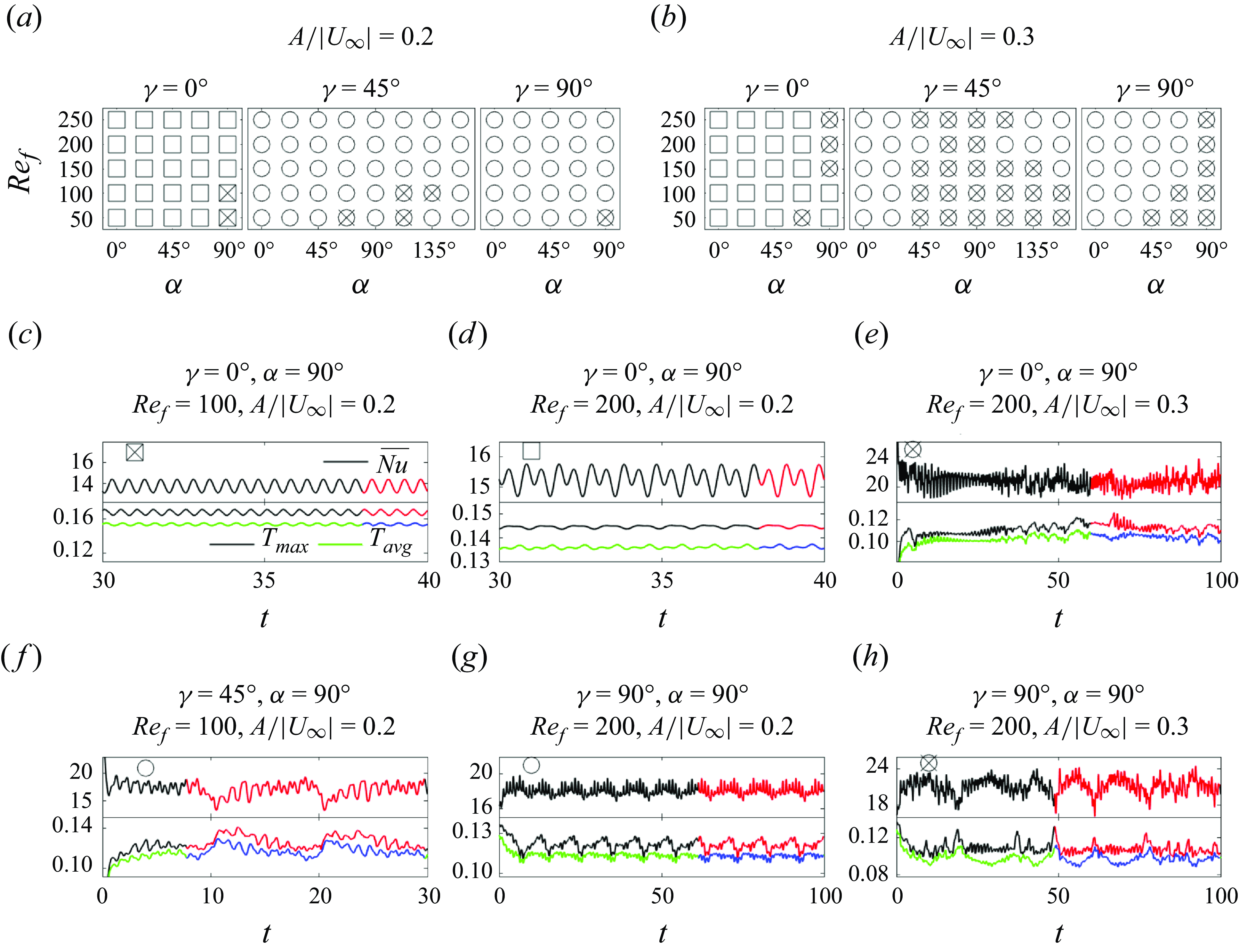
Figure 6. The four classes of the time series of $\overline {Nu}$
,
$\overline {Nu}$
, $T_{{avg}}$
and
$T_{{avg}}$
and $T_{max }$
. The three panels in (a) and (b) correspond to
$T_{max }$
. The three panels in (a) and (b) correspond to $\gamma =0^\circ$
,
$\gamma =0^\circ$
, $\gamma =45^\circ$
and
$\gamma =45^\circ$
and $\gamma =90^\circ$
, respectively. The open and filled squares denote period-1 and period-1/2 cases, respectively. The open and filled circles represent almost-periodic and non-periodic cases, respectively, with periods typically
$\gamma =90^\circ$
, respectively. The open and filled squares denote period-1 and period-1/2 cases, respectively. The open and filled circles represent almost-periodic and non-periodic cases, respectively, with periods typically $\gg 1$
in the almost-periodic cases. Panels (c)–(h) show examples of the four classes, with the class label at the upper left. The portion of the curves in red and blue is used to compute the time average.
$\gg 1$
in the almost-periodic cases. Panels (c)–(h) show examples of the four classes, with the class label at the upper left. The portion of the curves in red and blue is used to compute the time average.
The first major class corresponds to periodic time series, shown with squares. The squares are open for period-1 dynamics and filled with crosses for period-1/2 dynamics. To determine whether a case is periodic, we consider the last four cycles of the plate oscillation and compute the time average of $\overline {Nu}(t)$
and
$\overline {Nu}(t)$
and $T_{{avg}}(t)$
every half-cycle. We take the standard deviation of the eight values, normalised by
$T_{{avg}}(t)$
every half-cycle. We take the standard deviation of the eight values, normalised by ${1}/{4}\int _{t_{{end}}-4}^{t_{{end}}} \overline {Nu}(t) \, \textrm{d}t$
and
${1}/{4}\int _{t_{{end}}-4}^{t_{{end}}} \overline {Nu}(t) \, \textrm{d}t$
and ${1}/{4}\int _{t_{{end}}-4}^{t_{{end}}} T_{{avg}}(t) \, \textrm{d}t$
, respectively, with
${1}/{4}\int _{t_{{end}}-4}^{t_{{end}}} T_{{avg}}(t) \, \textrm{d}t$
, respectively, with $t_{{end}}$
the final time of the simulation. If the normalised standard deviation is below 0.1 % we label the case 1/2-periodic. If the case is not 1/2-periodic, we test for 1-periodicity by splitting the eight values into two groups, one for the first half-cycle and the other for the second half-cycle. If the average of the normalised standard deviations of each group is below 0.1 %, we label the case 1-periodic.
$t_{{end}}$
the final time of the simulation. If the normalised standard deviation is below 0.1 % we label the case 1/2-periodic. If the case is not 1/2-periodic, we test for 1-periodicity by splitting the eight values into two groups, one for the first half-cycle and the other for the second half-cycle. If the average of the normalised standard deviations of each group is below 0.1 %, we label the case 1-periodic.
Most cases with $\gamma =0^\circ$
(left sides of panels (a) and (b)) have period 1, i.e. the period of the plate oscillation. Period 1/2 occurs when the flow is symmetric on the two half-strokes of the plate, and this is possible only when the two half-strokes are symmetric with respect to the oncoming flow, i.e. for
$\gamma =0^\circ$
(left sides of panels (a) and (b)) have period 1, i.e. the period of the plate oscillation. Period 1/2 occurs when the flow is symmetric on the two half-strokes of the plate, and this is possible only when the two half-strokes are symmetric with respect to the oncoming flow, i.e. for $\alpha =90^\circ$
. Two cases with
$\alpha =90^\circ$
. Two cases with $\gamma =0^\circ$
,
$\gamma =0^\circ$
, $\alpha =90^\circ$
and
$\alpha =90^\circ$
and $A/|\boldsymbol{U}_{\infty }|=0.2$
have period 1/2 (filled squares), and the remainder have period 1.
$A/|\boldsymbol{U}_{\infty }|=0.2$
have period 1/2 (filled squares), and the remainder have period 1.
A period-1/2 example is shown in figure 6(c), and we will show the corresponding up–down symmetry of the vorticity field in § 4.2. Panel (d) shows an example with period 1 but not 1/2. Although the plate motion is up–down symmetric here, the flow is not. For all the periodic cases, we compute time averages using the last two plate oscillation cycles, e.g. the intervals marked in red and blue in panels (c) and (d).
The second major class corresponds to non-periodic time series, labelled with circles. In this class, the aforementioned normalised standard deviations based on the last four cycles of the plate oscillation are far above 0.1 %. All cases with $\gamma =45^\circ$
and
$\gamma =45^\circ$
and $90^\circ$
, and several cases with
$90^\circ$
, and several cases with $\gamma =0^\circ$
at
$\gamma =0^\circ$
at $A/|\boldsymbol{U}_{\infty }|=0.3$
, belong to this class. Within this class, open circles denote cases that are almost periodic with a period longer than 1. Figures 6(f) and 6(g) show examples of these cases. The time series have a component with the frequency of the plate oscillation and a much lower-frequency component, corresponding to 11 plate oscillations in figure 6(f) and 10 plate oscillations in figure 6(g). The low-frequency component is caused by the vortex grouping dynamics over several plate oscillation cycles, at almost the same location each time. We take time averages using at least two of these longer cycles of vortex grouping, shown in red and blue in panels (f) and (g).
$A/|\boldsymbol{U}_{\infty }|=0.3$
, belong to this class. Within this class, open circles denote cases that are almost periodic with a period longer than 1. Figures 6(f) and 6(g) show examples of these cases. The time series have a component with the frequency of the plate oscillation and a much lower-frequency component, corresponding to 11 plate oscillations in figure 6(f) and 10 plate oscillations in figure 6(g). The low-frequency component is caused by the vortex grouping dynamics over several plate oscillation cycles, at almost the same location each time. We take time averages using at least two of these longer cycles of vortex grouping, shown in red and blue in panels (f) and (g).
To quantitatively determine whether a case is almost periodic, we compare the cycle averages of $\overline {Nu}(t)$
and
$\overline {Nu}(t)$
and $T_{{avg}}(t)$
every
$T_{{avg}}(t)$
every $t_{{low}}$
apart for five consecutive oscillations, with
$t_{{low}}$
apart for five consecutive oscillations, with $t_{{low}}$
the tentative number of plate oscillations corresponding to the low-frequency component. For example, with
$t_{{low}}$
the tentative number of plate oscillations corresponding to the low-frequency component. For example, with $t_{{low}}=11$
in figure 6(f), the cycle-averaged
$t_{{low}}=11$
in figure 6(f), the cycle-averaged $\langle \overline {Nu} \rangle$
and
$\langle \overline {Nu} \rangle$
and $\langle T_{{avg}} \rangle$
from the 26th to 30th cycle are compared with those from the 15th to 19th cycle, respectively. We compute the standard deviations of the five pairs and then take the average and normalise it by
$\langle T_{{avg}} \rangle$
from the 26th to 30th cycle are compared with those from the 15th to 19th cycle, respectively. We compute the standard deviations of the five pairs and then take the average and normalise it by ${1}/{t_{{low}}}\int _{t_{{end}}-t_{{low}}}^{t_{{end}}} \overline {Nu}(t) \, \textrm{d}t$
and
${1}/{t_{{low}}}\int _{t_{{end}}-t_{{low}}}^{t_{{end}}} \overline {Nu}(t) \, \textrm{d}t$
and ${1}/{t_{{low}}}\int _{t_{{end}}-t_{{low}}}^{t_{{end}}} T_{{avg}}(t) \, \textrm{d}t$
, respectively. If the resulting value is
${1}/{t_{{low}}}\int _{t_{{end}}-t_{{low}}}^{t_{{end}}} T_{{avg}}(t) \, \textrm{d}t$
, respectively. If the resulting value is $\leqslant$
1 %, we label the case ‘almost periodic.’ In figure 6(f),
$\leqslant$
1 %, we label the case ‘almost periodic.’ In figure 6(f), $t_{{low}}=11$
, and the resulting two normalised average standard deviations are 0.67 % and 0.56 %, respectively. In figure 6(g), we have
$t_{{low}}=11$
, and the resulting two normalised average standard deviations are 0.67 % and 0.56 %, respectively. In figure 6(g), we have $t_{{low}}=10$
and the values are 0.26 % and 0.17 %. There are subtle but noticeable differences between the longer cycles that make these cases non-periodic: although the vortex configuration near the plate is nearly the same from one long period to the next, the configuration far from the plate differs. For this reason we chose the 1 % threshold for the almost-periodic cases, instead of the 0.1 % threshold for the periodic cases.
$t_{{low}}=10$
and the values are 0.26 % and 0.17 %. There are subtle but noticeable differences between the longer cycles that make these cases non-periodic: although the vortex configuration near the plate is nearly the same from one long period to the next, the configuration far from the plate differs. For this reason we chose the 1 % threshold for the almost-periodic cases, instead of the 0.1 % threshold for the periodic cases.
The last subclass, shown by circles with crosses, corresponds to a strongly non-periodic dynamics. In these cases, vortex grouping still occurs over long cycles, but the long cycles vary in duration, the positions of the groups vary from one long cycle to the next, and the vortex shedding can be irregular. These cases are more prevalent at $A/|\boldsymbol{U}_{\infty }|=0.3$
than 0.2, and with
$A/|\boldsymbol{U}_{\infty }|=0.3$
than 0.2, and with $\alpha$
close to
$\alpha$
close to $90^\circ$
, i.e. with more transverse plate motions. Such cases correspond to stronger vortices with a more complicated dynamics. Example time series are shown in figures 6(e) and 6(h). For this subclass we compute time averages over time intervals that are long enough that further increases give only minor changes, as shown in Appendix B. The beginnings and ends of the intervals are chosen so that the vorticity distributions near the plate approximately match.
$90^\circ$
, i.e. with more transverse plate motions. Such cases correspond to stronger vortices with a more complicated dynamics. Example time series are shown in figures 6(e) and 6(h). For this subclass we compute time averages over time intervals that are long enough that further increases give only minor changes, as shown in Appendix B. The beginnings and ends of the intervals are chosen so that the vorticity distributions near the plate approximately match.
We can interpret the periodic and almost-period cases by considering the frequency of vortex shedding due to the plate oscillation together with the natural wake shedding frequency seen in the steady cases of § 3 at $\gamma = 45^\circ$
and
$\gamma = 45^\circ$
and $90^\circ$
. At
$90^\circ$
. At $\gamma = 0^\circ$
there is no natural wake shedding frequency, so here the dynamics is mostly periodic with the period of the plate oscillation. At
$\gamma = 0^\circ$
there is no natural wake shedding frequency, so here the dynamics is mostly periodic with the period of the plate oscillation. At $\gamma = 45^\circ$
and
$\gamma = 45^\circ$
and $90^\circ$
there is the additional wake frequency, but many cases are close to periodic, particularly at
$90^\circ$
there is the additional wake frequency, but many cases are close to periodic, particularly at $A/|\boldsymbol{U}_{\infty }|$
= 0.2. Such cases resemble frequency locking between the wake and plate oscillation, which has been studied most often for circular cylinders (Koopmann Reference Koopmann1967; Armstrong, Barnes & Grant Reference Armstrong, Barnes and Grant1986; Williamson & Roshko Reference Williamson and Roshko1988; Chen & Fang Reference Chen and Fang1998). In these studies, lock-in was observed when the body was forced at a period within approximately 20 % of the natural wake period. Locking of the flow to a multiple of the period of the oscillating body was found in experiments by Bishop & Hassan (Reference Bishop and Hassan1964) and in computations of an oscillating ellipse that is free to translate horizontally (Alben Reference Alben2008).
$A/|\boldsymbol{U}_{\infty }|$
= 0.2. Such cases resemble frequency locking between the wake and plate oscillation, which has been studied most often for circular cylinders (Koopmann Reference Koopmann1967; Armstrong, Barnes & Grant Reference Armstrong, Barnes and Grant1986; Williamson & Roshko Reference Williamson and Roshko1988; Chen & Fang Reference Chen and Fang1998). In these studies, lock-in was observed when the body was forced at a period within approximately 20 % of the natural wake period. Locking of the flow to a multiple of the period of the oscillating body was found in experiments by Bishop & Hassan (Reference Bishop and Hassan1964) and in computations of an oscillating ellipse that is free to translate horizontally (Alben Reference Alben2008).
Although it might be conjectured that the four classes correspond to completely different heat transfer performances, we do not see a direct mechanism by which one class performs better than the other consistently. In particular, as we will show next, it is not uncommon for different classes to have similar global heat transfer. Thus the classification only indicates the regularity of the vortex dynamics. In the following discussion, we can see that, compared with the regularity of the vortex dynamics, the strength of the shed vorticity is more correlated with heat transfer.
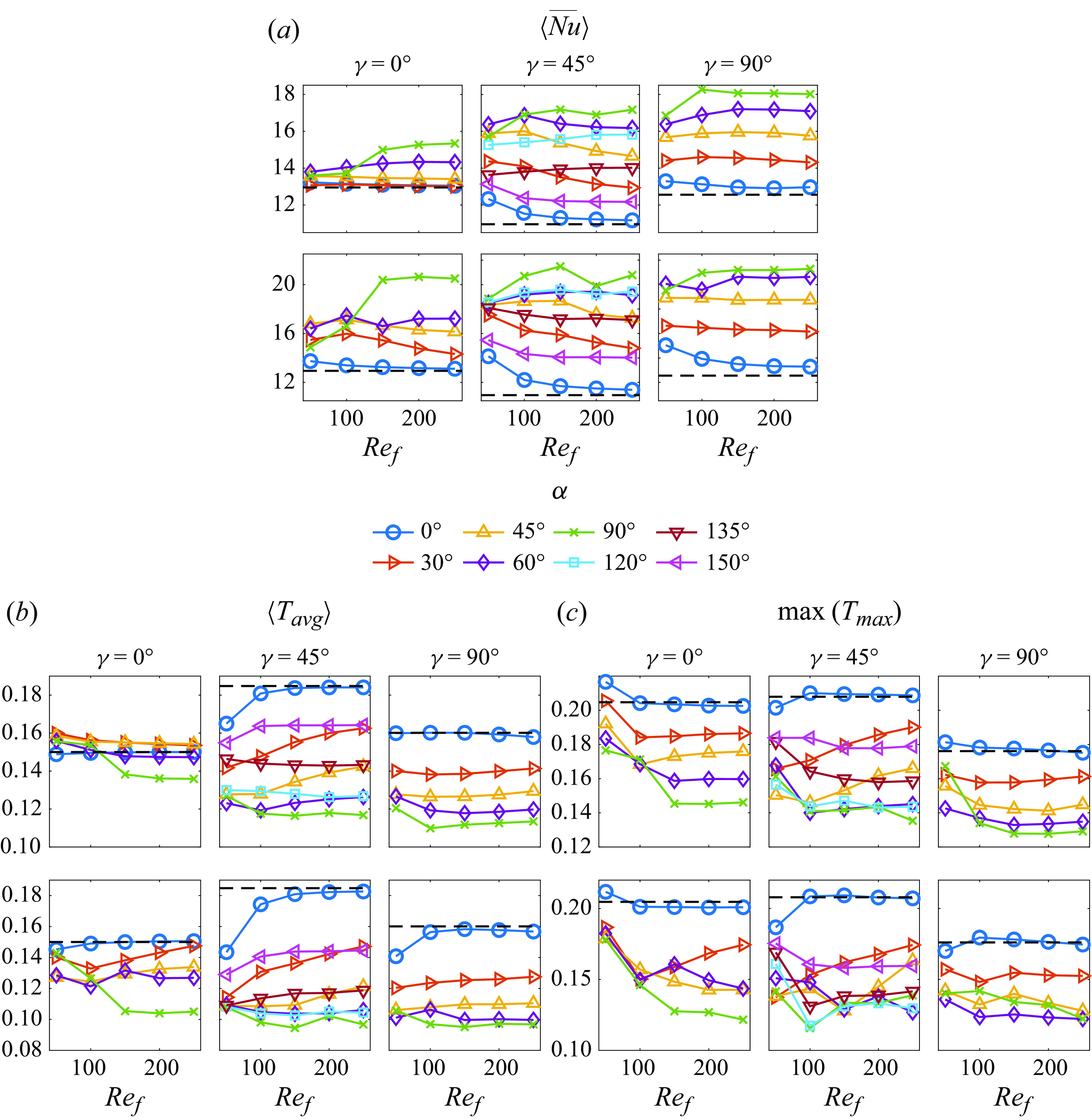
Figure 7. (a) The time-averaged global Nusselt number, $\langle \overline {Nu}\rangle$
, for the isothermal plate, (b) the time-averaged plate temperature,
$\langle \overline {Nu}\rangle$
, for the isothermal plate, (b) the time-averaged plate temperature, $\langle T_{{avg}} \rangle$
and (c) the maximum plate temperature,
$\langle T_{{avg}} \rangle$
and (c) the maximum plate temperature, $\max (T_{max })$
, when the heat flux from the plate is fixed. The first and second rows in each panel correspond to
$\max (T_{max })$
, when the heat flux from the plate is fixed. The first and second rows in each panel correspond to $A/|\boldsymbol{U}_{\infty }|=0.2$
and 0.3, respectively. The dashed line in each panel gives the values for the non-oscillating plate. The panels in the same row share the same
$A/|\boldsymbol{U}_{\infty }|=0.2$
and 0.3, respectively. The dashed line in each panel gives the values for the non-oscillating plate. The panels in the same row share the same $y$
axis for ease of comparison.
$y$
axis for ease of comparison.
Having classified the types of dynamics over the full parameter space in figures 6(a) and 6(b), we plot the key global measures of heat transfer in the same parameter space in figure 7. Panels (a) and (b) show the time- and space-averaged Nusselt number $\langle \overline {Nu} \rangle$
and plate temperature
$\langle \overline {Nu} \rangle$
and plate temperature $\langle T_{{avg}} \rangle$
in the fixed-temperature and fixed-flux cases respectively. In the latter case, panel (c) shows the maximum plate temperature over space and time,
$\langle T_{{avg}} \rangle$
in the fixed-temperature and fixed-flux cases respectively. In the latter case, panel (c) shows the maximum plate temperature over space and time, $\max (T_{max })$
. Instead of 2-D plots in the (
$\max (T_{max })$
. Instead of 2-D plots in the ( $Re_f$
,
$Re_f$
, $\alpha$
) space of figure 6, figure 7 plots each quantity versus
$\alpha$
) space of figure 6, figure 7 plots each quantity versus $Re_f$
with a separate line for each
$Re_f$
with a separate line for each $\alpha$
, so that we can compare the values of the quantities clearly by referring to the vertical axes.
$\alpha$
, so that we can compare the values of the quantities clearly by referring to the vertical axes.
Comparing figures 7(a) and 7(b) we see that $\langle \overline {Nu} \rangle$
and
$\langle \overline {Nu} \rangle$
and $\langle T_{{avg}} \rangle$
are generally anticorrelated as
$\langle T_{{avg}} \rangle$
are generally anticorrelated as $Re_f$
and
$Re_f$
and $\alpha$
vary, i.e. the two quantities give the same ordering of parameters in terms of optimality for heat transfer. Here,
$\alpha$
vary, i.e. the two quantities give the same ordering of parameters in terms of optimality for heat transfer. Here, $\max (T_{max })$
is generally consistent with this ordering but shows more deviations, because it is more sensitive to the details of the velocity and temperature field evolution near the particular instant when the maximum temperature occurs.
$\max (T_{max })$
is generally consistent with this ordering but shows more deviations, because it is more sensitive to the details of the velocity and temperature field evolution near the particular instant when the maximum temperature occurs.
Now we discuss the effect of each of the four key parameters – $A/|\boldsymbol{U}_{\infty }|$
,
$A/|\boldsymbol{U}_{\infty }|$
, $\alpha$
,
$\alpha$
, $\gamma$
and
$\gamma$
and $Re_f$
– on global (time- and space-averaged) heat transfer, and the role of the vortex dynamics. Since the heat transfer enhancement is realised through oscillation-induced vortices, we expect a positive correlation between the vorticity strength near the plate and the global heat transfer. In Appendix D, we show the time-averaged vorticity strength, defined as the integral of the absolute value of the vorticity within a box around the plate, as
$Re_f$
– on global (time- and space-averaged) heat transfer, and the role of the vortex dynamics. Since the heat transfer enhancement is realised through oscillation-induced vortices, we expect a positive correlation between the vorticity strength near the plate and the global heat transfer. In Appendix D, we show the time-averaged vorticity strength, defined as the integral of the absolute value of the vorticity within a box around the plate, as $A/|\boldsymbol{U}_{\infty }|$
,
$A/|\boldsymbol{U}_{\infty }|$
, $\alpha$
,
$\alpha$
, $\gamma$
and
$\gamma$
and $Re_f$
vary. It is confirmed that the vorticity strength is strongly correlated with global heat transfer as the parameters vary. In the next subsection, we will present detailed descriptions of the vorticity distributions across space and time, and the corresponding local distributions of heat transfer quantities that underlie the global patterns.
$Re_f$
vary. It is confirmed that the vorticity strength is strongly correlated with global heat transfer as the parameters vary. In the next subsection, we will present detailed descriptions of the vorticity distributions across space and time, and the corresponding local distributions of heat transfer quantities that underlie the global patterns.
Consistent with Rahman & Tafti (Reference Rahman and Tafti2020a
), we find $A/|\boldsymbol{U}_{\infty }| = 0.3$
(bottom rows of each panel) gives better global heat transfer—larger
$A/|\boldsymbol{U}_{\infty }| = 0.3$
(bottom rows of each panel) gives better global heat transfer—larger $\langle \overline {Nu} \rangle$
and smaller
$\langle \overline {Nu} \rangle$
and smaller $\langle T_{{avg}} \rangle$
—than 0.2 (top rows), if the other parameters are the same. The extent of the improvement varies with
$\langle T_{{avg}} \rangle$
—than 0.2 (top rows), if the other parameters are the same. The extent of the improvement varies with $\alpha$
,
$\alpha$
, $\gamma$
and
$\gamma$
and $Re_f$
. Larger
$Re_f$
. Larger $A/|\boldsymbol{U}_{\infty }|$
means larger plate velocity and stronger vorticity generation (as shown in figure 25 in Appendix D), which tend to bring colder fluid close to the plate.
$A/|\boldsymbol{U}_{\infty }|$
means larger plate velocity and stronger vorticity generation (as shown in figure 25 in Appendix D), which tend to bring colder fluid close to the plate.
By comparing different coloured lines within each panel we see the effect of varying the plate oscillation direction $\alpha$
. At
$\alpha$
. At $\gamma = 45^\circ$
and
$\gamma = 45^\circ$
and $90^\circ$
, the three metrics vary by a factor of 1.5–2 as
$90^\circ$
, the three metrics vary by a factor of 1.5–2 as $\alpha$
is varied, with smaller variation at
$\alpha$
is varied, with smaller variation at $\gamma = 0^\circ$
. In most cases
$\gamma = 0^\circ$
. In most cases $\alpha$
has a stronger effect than
$\alpha$
has a stronger effect than $A/|\boldsymbol{U}_{\infty }|$
with other parameters fixed. Transverse oscillation (
$A/|\boldsymbol{U}_{\infty }|$
with other parameters fixed. Transverse oscillation ( $\alpha =90^\circ$
) generally gives the best heat transfer (highest
$\alpha =90^\circ$
) generally gives the best heat transfer (highest $\langle \overline {Nu} \rangle$
and lowest
$\langle \overline {Nu} \rangle$
and lowest $\langle T_{{avg}}\rangle$
) and in-plane oscillation (
$\langle T_{{avg}}\rangle$
) and in-plane oscillation ( $\alpha =0^\circ$
) is generally worst, except for a few cases at low
$\alpha =0^\circ$
) is generally worst, except for a few cases at low $Re_f$
. The lowest
$Re_f$
. The lowest $\max (T_{max })$
generally occurs at
$\max (T_{max })$
generally occurs at $\alpha = 90^\circ$
also, or at nearby values (
$\alpha = 90^\circ$
also, or at nearby values ( $60^\circ$
or
$60^\circ$
or $120^\circ$
).
$120^\circ$
).
These dependences on $\alpha$
and other, more subtle, effects are connected to the vortex dynamics. First, the plate generates stronger vortices when
$\alpha$
and other, more subtle, effects are connected to the vortex dynamics. First, the plate generates stronger vortices when $\alpha$
is closer to
$\alpha$
is closer to $90^\circ$
(i.e. the oscillation is more transverse than in plane). (In Appendix D, we show that the vorticity strength increases as
$90^\circ$
(i.e. the oscillation is more transverse than in plane). (In Appendix D, we show that the vorticity strength increases as $\alpha$
approaches
$\alpha$
approaches $90^\circ$
.) This generally enhances local heat transfer in the wake, as discussed in § 4.2. Some exceptions are seen, e.g. in panel (b), the fixed-heat-flux cases, in the top left subpanel (
$90^\circ$
.) This generally enhances local heat transfer in the wake, as discussed in § 4.2. Some exceptions are seen, e.g. in panel (b), the fixed-heat-flux cases, in the top left subpanel ( $\gamma =0^\circ$
and
$\gamma =0^\circ$
and $A/|\boldsymbol{U}_{\infty }|=0.2$
). Here,
$A/|\boldsymbol{U}_{\infty }|=0.2$
). Here, $\alpha =30^\circ$
and
$\alpha =30^\circ$
and $45^\circ$
have higher
$45^\circ$
have higher $\langle T_{{avg}} \rangle$
than
$\langle T_{{avg}} \rangle$
than $\alpha =0^\circ$
, while
$\alpha =0^\circ$
, while $\max (T_{max })$
is more monotonic with
$\max (T_{max })$
is more monotonic with $\alpha$
. The vorticity fields at
$\alpha$
. The vorticity fields at $\alpha =30^\circ$
and
$\alpha =30^\circ$
and $45^\circ$
create a more uniform thermal boundary layer with a lower maximum temperature but a higher average temperature than
$45^\circ$
create a more uniform thermal boundary layer with a lower maximum temperature but a higher average temperature than $\alpha =0^\circ$
.
$\alpha =0^\circ$
.
At $\gamma =45^\circ$
,
$\gamma =45^\circ$
, $\alpha$
spans the range
$\alpha$
spans the range $[0^\circ , 180^\circ )$
, unlike
$[0^\circ , 180^\circ )$
, unlike $\gamma =0^\circ$
and
$\gamma =0^\circ$
and $90^\circ$
which have the (
$90^\circ$
which have the ( $\alpha \leftrightarrow 180^\circ -\alpha$
) symmetry. For
$\alpha \leftrightarrow 180^\circ -\alpha$
) symmetry. For $\gamma =45^\circ$
, the eight
$\gamma =45^\circ$
, the eight $\alpha$
values form five groups in order of proximity to 90
$\alpha$
values form five groups in order of proximity to 90 $^\circ$
: 90
$^\circ$
: 90 $^\circ$
, 60
$^\circ$
, 60 $^\circ$
/120
$^\circ$
/120 $^\circ$
, 45
$^\circ$
, 45 $^\circ$
/135
$^\circ$
/135 $^\circ$
, 30
$^\circ$
, 30 $^\circ$
/150
$^\circ$
/150 $^\circ$
and 0
$^\circ$
and 0 $^\circ$
. We have already mentioned that heat transfer increases with proximity to 90
$^\circ$
. We have already mentioned that heat transfer increases with proximity to 90 $^\circ$
, but there is an additional variation within the three pairs. The plate oscillation is more in plane with the oncoming flow for the first member of each pair (
$^\circ$
, but there is an additional variation within the three pairs. The plate oscillation is more in plane with the oncoming flow for the first member of each pair ( $\alpha \lt 90^\circ$
) and more transverse for the second (
$\alpha \lt 90^\circ$
) and more transverse for the second ( $\alpha \gt 90^\circ$
), e.g.
$\alpha \gt 90^\circ$
), e.g. $\alpha = 45$
versus
$\alpha = 45$
versus $135^\circ$
with
$135^\circ$
with $\gamma = 45^\circ$
in figure 1. Comparing the graphs for each pair in figure 7, we usually have better global heat transfer for in-plane oscillation, but the difference becomes smaller as
$\gamma = 45^\circ$
in figure 1. Comparing the graphs for each pair in figure 7, we usually have better global heat transfer for in-plane oscillation, but the difference becomes smaller as $Re_f$
or
$Re_f$
or $A/|\boldsymbol{U}_{\infty }|$
increases. For example,
$A/|\boldsymbol{U}_{\infty }|$
increases. For example, $\langle \overline {Nu} \rangle$
is larger and
$\langle \overline {Nu} \rangle$
is larger and $\langle T_{{avg}} \rangle$
is smaller with
$\langle T_{{avg}} \rangle$
is smaller with $\alpha =60^\circ$
than
$\alpha =60^\circ$
than $\alpha =120^\circ$
at
$\alpha =120^\circ$
at $\gamma =45^\circ$
and
$\gamma =45^\circ$
and $A/|\boldsymbol{U}_{\infty }|=0.2$
(top centre subpanels of (a) and (b)), and the difference between the two becomes smaller at higher
$A/|\boldsymbol{U}_{\infty }|=0.2$
(top centre subpanels of (a) and (b)), and the difference between the two becomes smaller at higher $Re_f$
, and is almost non-existent at
$Re_f$
, and is almost non-existent at $A/|\boldsymbol{U}_{\infty }|$
= 0.3 (bottom centre subpanels of (a) and (b)). A short explanation for this phenomenon is that oscillating along the flow (
$A/|\boldsymbol{U}_{\infty }|$
= 0.3 (bottom centre subpanels of (a) and (b)). A short explanation for this phenomenon is that oscillating along the flow ( $\alpha \lt 90^\circ$
) generates stronger vortices than oscillating across the flow (
$\alpha \lt 90^\circ$
) generates stronger vortices than oscillating across the flow ( $\alpha \gt 90^\circ$
), as shown by figure 25 in Appendix D. In the next section we will discuss the differences between the vortex dynamics that underlie these results.
$\alpha \gt 90^\circ$
), as shown by figure 25 in Appendix D. In the next section we will discuss the differences between the vortex dynamics that underlie these results.
The plate orientation $\gamma$
generally has a weaker effect on heat transfer than
$\gamma$
generally has a weaker effect on heat transfer than $\alpha$
and
$\alpha$
and $A/|\boldsymbol{U}_{\infty }|$
, particularly when we focus on the variations with
$A/|\boldsymbol{U}_{\infty }|$
, particularly when we focus on the variations with $\gamma$
when
$\gamma$
when $\alpha = 90^\circ$
in figure 7 (the green curves), usually the best
$\alpha = 90^\circ$
in figure 7 (the green curves), usually the best $\alpha$
for heat transfer. At
$\alpha$
for heat transfer. At $A/|\boldsymbol{U}_{\infty }|$
= 0.2 (top rows),
$A/|\boldsymbol{U}_{\infty }|$
= 0.2 (top rows), $\langle \overline {Nu} \rangle$
is lowest at
$\langle \overline {Nu} \rangle$
is lowest at $\gamma = 0^\circ$
, where the flow is periodic with period 1 and has an attached vortex group near the leading edge of the bottom wall that decreases local heat transfer. By contrast, the flows for
$\gamma = 0^\circ$
, where the flow is periodic with period 1 and has an attached vortex group near the leading edge of the bottom wall that decreases local heat transfer. By contrast, the flows for $\gamma =45^\circ$
and
$\gamma =45^\circ$
and $90^\circ$
are non-periodic, with alternating formations of vortex groups at both edges of the plate’s top wall over many plate oscillation cycles, which improves the local (and global) heat transfer. We will give examples in § 4.2.
$90^\circ$
are non-periodic, with alternating formations of vortex groups at both edges of the plate’s top wall over many plate oscillation cycles, which improves the local (and global) heat transfer. We will give examples in § 4.2.
At $A/|\boldsymbol{U}_{\infty }| = 0.3$
, by contrast, the maximum
$A/|\boldsymbol{U}_{\infty }| = 0.3$
, by contrast, the maximum $\langle \overline {Nu} \rangle$
and minimum
$\langle \overline {Nu} \rangle$
and minimum $\langle T_{{avg}} \rangle$
are approximately the same for all three
$\langle T_{{avg}} \rangle$
are approximately the same for all three $\gamma$
values, as shown in the bottom rows of each subpanel. All of these cases are non-periodic and involve long-lasting groups of strong vortices at the plate edges. Here, different
$\gamma$
values, as shown in the bottom rows of each subpanel. All of these cases are non-periodic and involve long-lasting groups of strong vortices at the plate edges. Here, different $\gamma$
yield different vortex group positions that enhance heat transfer in different locations, but the global heat transfer performance is similar, as we will show in § 4.2.
$\gamma$
yield different vortex group positions that enhance heat transfer in different locations, but the global heat transfer performance is similar, as we will show in § 4.2.
Surprisingly, the global heat transfer quantities do not vary much with $Re_f$
in most cases i.e. most curves in figure 7 are nearly flat, particularly at
$Re_f$
in most cases i.e. most curves in figure 7 are nearly flat, particularly at $Re_f$
above 100. Recall from the beginning of § 4 that we vary
$Re_f$
above 100. Recall from the beginning of § 4 that we vary $Re_f$
by keeping the oscillation velocity
$Re_f$
by keeping the oscillation velocity $A/|\boldsymbol{U}_{\infty }|$
fixed, so for each graph in figure 7, increasing the frequency
$A/|\boldsymbol{U}_{\infty }|$
fixed, so for each graph in figure 7, increasing the frequency $Re_f$
decreases the amplitude
$Re_f$
decreases the amplitude $A$
such that the product is fixed. (Also, as shown in figure 25 in Appendix D, vorticity strength does not vary strongly with
$A$
such that the product is fixed. (Also, as shown in figure 25 in Appendix D, vorticity strength does not vary strongly with $Re_f$
in most cases.) As we will see in § 4.2, the vortex dynamics and the resulting local heat transfer do not vary much as
$Re_f$
in most cases.) As we will see in § 4.2, the vortex dynamics and the resulting local heat transfer do not vary much as $Re_f$
increases. An exception is
$Re_f$
increases. An exception is $\gamma =0^\circ$
and
$\gamma =0^\circ$
and $\alpha =90^\circ$
(green curves). In the leftmost subpanels, the green curves jump when
$\alpha =90^\circ$
(green curves). In the leftmost subpanels, the green curves jump when $Re_f$
increases from 100 to 150, showing improved heat transfer. These jumps correspond to flow transitions: the transition from period-1/2 to period-1 dynamics at
$Re_f$
increases from 100 to 150, showing improved heat transfer. These jumps correspond to flow transitions: the transition from period-1/2 to period-1 dynamics at $A/|\boldsymbol{U}_{\infty }|=0.2$
due to symmetry breaking, and the transition from period-1 to non-periodic dynamics at
$A/|\boldsymbol{U}_{\infty }|=0.2$
due to symmetry breaking, and the transition from period-1 to non-periodic dynamics at $A/|\boldsymbol{U}_{\infty }|=0.3$
. With each transition, stronger vortices are generated by means of vortex grouping (see figure 25 in Appendix D), and local and global heat transfer are enhanced, as described in § 4.2. At other parameters (e.g.
$A/|\boldsymbol{U}_{\infty }|=0.3$
. With each transition, stronger vortices are generated by means of vortex grouping (see figure 25 in Appendix D), and local and global heat transfer are enhanced, as described in § 4.2. At other parameters (e.g. $\gamma = 45^\circ$
and
$\gamma = 45^\circ$
and $90^\circ$
), the curves also jump between
$90^\circ$
), the curves also jump between $Re_f$
= 50 and 100. These changes also correspond to transitions in the vortex dynamics. In particular, vortex grouping is enhanced as
$Re_f$
= 50 and 100. These changes also correspond to transitions in the vortex dynamics. In particular, vortex grouping is enhanced as $Re_f$
increases from 50 to 100 so that stronger vortices are trapped near the plate, increasing local and global heat transfer at
$Re_f$
increases from 50 to 100 so that stronger vortices are trapped near the plate, increasing local and global heat transfer at $Re_f=100$
. In Appendix D, we compare the vortex dynamics between
$Re_f=100$
. In Appendix D, we compare the vortex dynamics between $Re_f$
= 50 and 100 with
$Re_f$
= 50 and 100 with $\gamma = 45^\circ$
and
$\gamma = 45^\circ$
and $90^\circ$
in figure 26 and 27, respectively, to illustrate this point.
$90^\circ$
in figure 26 and 27, respectively, to illustrate this point.
4.2. Local heat transfer
In the previous section we summarised the general trends of the vorticity dynamics and heat transfer in terms of time- and space-averaged (global) quantities. Now we show the vorticity and temperature fields and the heat flux and temperature distributions on the plate that explain these trends, in the space of the four key parameters: $A/|\boldsymbol{U}_{\infty }|$
,
$A/|\boldsymbol{U}_{\infty }|$
, $\alpha$
,
$\alpha$
, $\gamma$
and
$\gamma$
and $Re_f$
. Since the temperature fields are similar for the isothermal and fixed-heat-flux plates (also seen in figures 4(a), 4(b) and 5), we only show the temperature fields for the isothermal plate in this section.
$Re_f$
. Since the temperature fields are similar for the isothermal and fixed-heat-flux plates (also seen in figures 4(a), 4(b) and 5), we only show the temperature fields for the isothermal plate in this section.
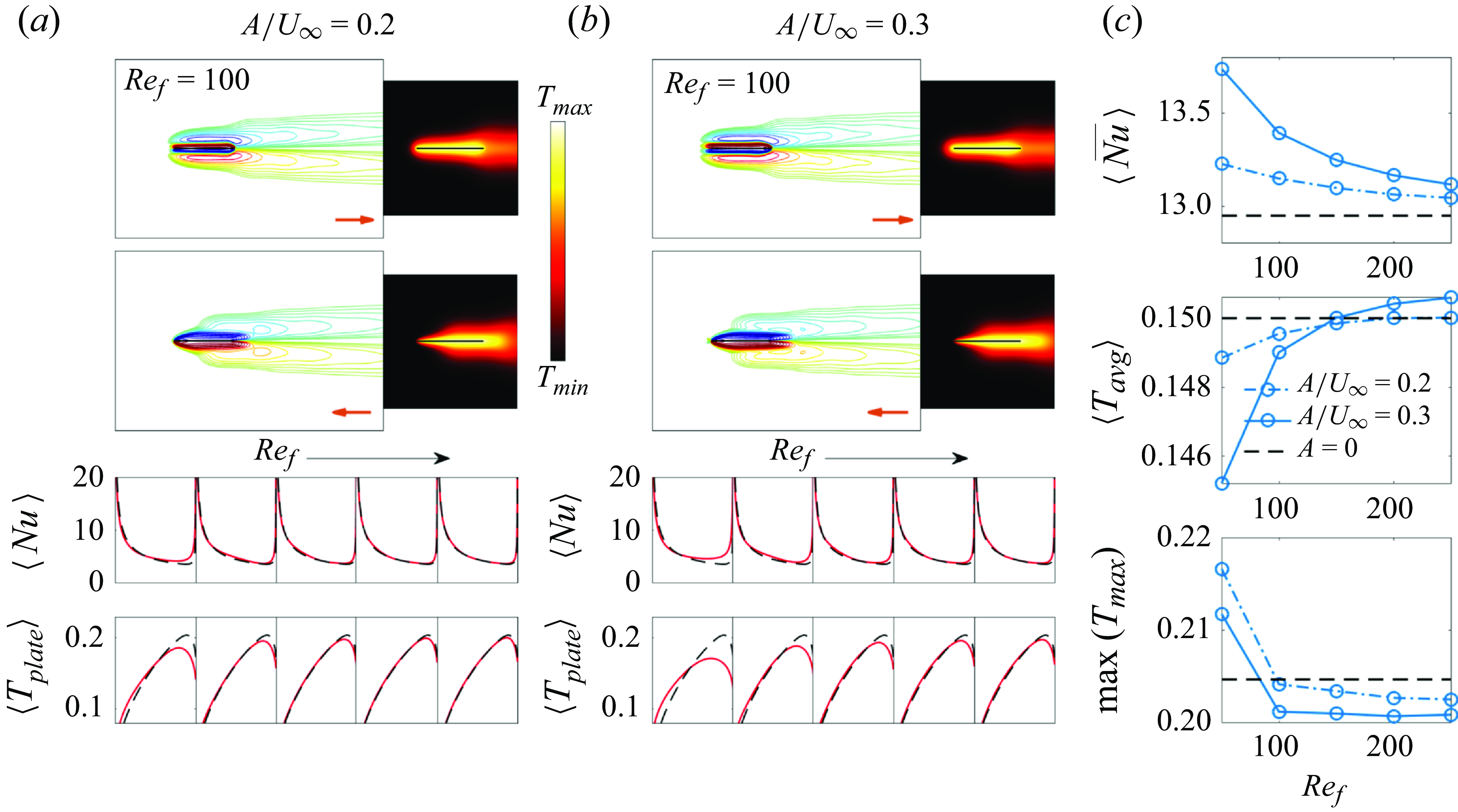
Figure 8. Flows and heat transfer for in-plane plate oscillation ( $\alpha = 0^\circ$
) in an in-plane oncoming flow (
$\alpha = 0^\circ$
) in an in-plane oncoming flow ( $\gamma =0^\circ$
). Panels (a) and (b) show vorticity and temperature fields (in the first two rows) at
$\gamma =0^\circ$
). Panels (a) and (b) show vorticity and temperature fields (in the first two rows) at $Re_f = 100$
, the time-averaged local
$Re_f = 100$
, the time-averaged local $Nu$
with fixed plate temperature (red lines in the third row) and the time-averaged plate temperature with fixed heat flux (red lines in the fourth row). The red arrows in the vorticity snapshots indicate the instantaneous plate velocity direction. The motion in panel (b) is shown in the supplementary movie 1, accessible https://doi.org/10.1017/jfm.2025.10201. Panel (c) shows time-averaged global heat transfer quantities. In each panel the black dashed lines are the non-oscillating-plate results.
$Nu$
with fixed plate temperature (red lines in the third row) and the time-averaged plate temperature with fixed heat flux (red lines in the fourth row). The red arrows in the vorticity snapshots indicate the instantaneous plate velocity direction. The motion in panel (b) is shown in the supplementary movie 1, accessible https://doi.org/10.1017/jfm.2025.10201. Panel (c) shows time-averaged global heat transfer quantities. In each panel the black dashed lines are the non-oscillating-plate results.
4.2.1. In-plane oncoming flow: $\gamma =0^\circ$

We start with in-plane plate oscillation ( $\alpha = 0^\circ$
) in an in-plane oncoming flow (
$\alpha = 0^\circ$
) in an in-plane oncoming flow ( $\gamma =0^\circ$
). These are the only cases without significant vortex shedding and thus have the smallest change in heat transfer due to plate motion.
$\gamma =0^\circ$
). These are the only cases without significant vortex shedding and thus have the smallest change in heat transfer due to plate motion.
The top panels of figures 8(a) and 8(b) show the vorticity and temperatures fields for $A/|\boldsymbol{U}_{\infty }| =0.2$
and
$A/|\boldsymbol{U}_{\infty }| =0.2$
and $A/|\boldsymbol{U}_{\infty }| =0.3$
, respectively, at the instants of maximum rightward and leftward velocity, shown by the red arrows. The attached shear layers and vortex wakes are slightly different from those without plate motion (figure 4
a), but still up–down symmetric. When the plate moves to the right (top row), the thermal boundary layer is more uniform than for the steady plate, and heat flux is reduced near the leading edge. When the plate moves to the left (second row), the larger velocity difference with the oncoming flow reduces the thermal boundary thickness near the leading edge, increasing the heat flux there.
$A/|\boldsymbol{U}_{\infty }| =0.3$
, respectively, at the instants of maximum rightward and leftward velocity, shown by the red arrows. The attached shear layers and vortex wakes are slightly different from those without plate motion (figure 4
a), but still up–down symmetric. When the plate moves to the right (top row), the thermal boundary layer is more uniform than for the steady plate, and heat flux is reduced near the leading edge. When the plate moves to the left (second row), the larger velocity difference with the oncoming flow reduces the thermal boundary thickness near the leading edge, increasing the heat flux there.
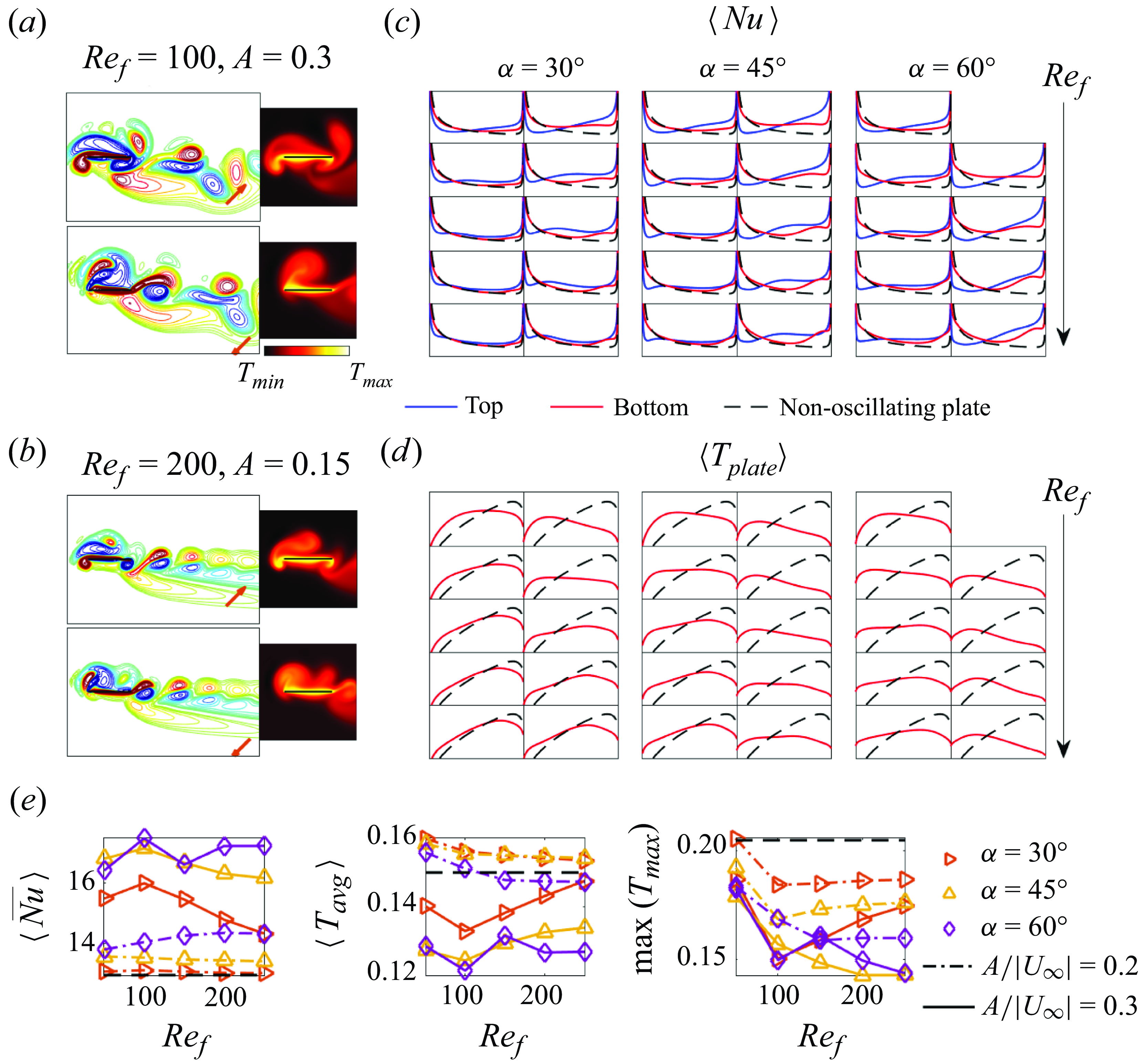
Figure 9. Flows and heat transfer for oblique plate oscillation ( $\alpha = 30^\circ , 45^\circ$
and
$\alpha = 30^\circ , 45^\circ$
and $60^\circ$
) in an in-plane oncoming flow (
$60^\circ$
) in an in-plane oncoming flow ( $\gamma =0^\circ$
). Panels (a) and (b) show snapshots of the vorticity and temperature field at
$\gamma =0^\circ$
). Panels (a) and (b) show snapshots of the vorticity and temperature field at $\alpha = 45^\circ$
and
$\alpha = 45^\circ$
and $\gamma =0^\circ$
. The motion in panel (b) is shown in the supplementary movie 2, accessible here. The red arrows in the vorticity snapshots show the instantaneous plate velocity direction. Panels (c) and (d) show the time-averaged local
$\gamma =0^\circ$
. The motion in panel (b) is shown in the supplementary movie 2, accessible here. The red arrows in the vorticity snapshots show the instantaneous plate velocity direction. Panels (c) and (d) show the time-averaged local $Nu$
and plate-temperature distributions versus
$Nu$
and plate-temperature distributions versus $x$
(the horizontal axis) when the plate temperature or heat flux is fixed, respectively. The graphs are arranged in three columns, one for each
$x$
(the horizontal axis) when the plate temperature or heat flux is fixed, respectively. The graphs are arranged in three columns, one for each $\alpha$
, and five rows, one for each
$\alpha$
, and five rows, one for each $Re_f$
from 50 to 250, increasing downward. Pairs of subpanels are shown in each column, corresponding to
$Re_f$
from 50 to 250, increasing downward. Pairs of subpanels are shown in each column, corresponding to $A/|\boldsymbol{U}_{\infty }| =0.2$
and 0.3 on the left and right, respectively. Panel (e) shows the global heat transfer quantities; here
$A/|\boldsymbol{U}_{\infty }| =0.2$
and 0.3 on the left and right, respectively. Panel (e) shows the global heat transfer quantities; here $\langle \overline {Nu} \rangle$
and
$\langle \overline {Nu} \rangle$
and $\langle T_{{avg}} \rangle$
are the spatial averages of the graphs in panels (c) and (d) (and summing the top and bottom values of
$\langle T_{{avg}} \rangle$
are the spatial averages of the graphs in panels (c) and (d) (and summing the top and bottom values of $\langle Nu \rangle$
for
$\langle Nu \rangle$
for $\langle \overline {Nu} \rangle$
). In all cases the black dashed lines show the results for the non-oscillating plate.
$\langle \overline {Nu} \rangle$
). In all cases the black dashed lines show the results for the non-oscillating plate.
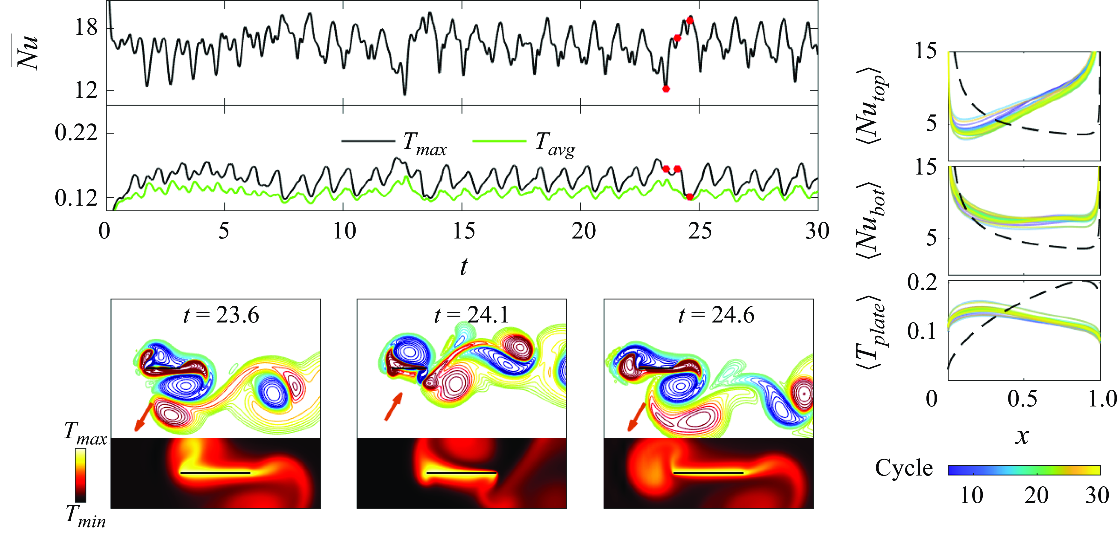
Figure 10. The non-periodic case with $\gamma =0^\circ$
,
$\gamma =0^\circ$
, $\alpha = 60^\circ$
,
$\alpha = 60^\circ$
, $Re_f=50$
and
$Re_f=50$
and $A/{|\boldsymbol{U}|_{\infty }}=0.3$
. The three snapshots of the vorticity and temperature field correspond to times marked with red dots on the graphs of
$A/{|\boldsymbol{U}|_{\infty }}=0.3$
. The three snapshots of the vorticity and temperature field correspond to times marked with red dots on the graphs of $ \overline {Nu}$
and
$ \overline {Nu}$
and $\langle T_{{max}} \rangle$
. The red arrows in the vorticity snapshots show the instantaneous direction of plate motion. The right three panels show the cycle-averaged
$\langle T_{{max}} \rangle$
. The red arrows in the vorticity snapshots show the instantaneous direction of plate motion. The right three panels show the cycle-averaged $\langle Nu \rangle$
of the top and bottom walls for the isothermal plate, and the cycle-averaged
$\langle Nu \rangle$
of the top and bottom walls for the isothermal plate, and the cycle-averaged $\langle T_{{plate}} \rangle$
with fixed heat flux. The first 5 cycles are omitted to avoid transient effects. The black dashed line shows the results for the non-oscillating plate. This motion is shown in the supplementary movie 3, accessible here.
$\langle T_{{plate}} \rangle$
with fixed heat flux. The first 5 cycles are omitted to avoid transient effects. The black dashed line shows the results for the non-oscillating plate. This motion is shown in the supplementary movie 3, accessible here.
The third and fourth rows of panels (a) and (b) show that the time-averaged quantities $\langle Nu \rangle$
and
$\langle Nu \rangle$
and $\langle T_{{plate}} \rangle$
(red lines) are slightly worse near the leading edge and slightly better near the trailing edge than the steady case (black dashed lines), and the difference diminishes as
$\langle T_{{plate}} \rangle$
(red lines) are slightly worse near the leading edge and slightly better near the trailing edge than the steady case (black dashed lines), and the difference diminishes as $Re_f$
increases. Here,
$Re_f$
increases. Here, $Nu$
denotes
$Nu$
denotes $Nu_{{top}}$
and
$Nu_{{top}}$
and $Nu_{{bot}}$
, equal by symmetry. As
$Nu_{{bot}}$
, equal by symmetry. As $Re_f$
increases, the vorticity fields and
$Re_f$
increases, the vorticity fields and $\langle \overline {Nu} \rangle$
(panel (c)) are closer to the steady values. The lower two subpanels of (c) show that, interestingly,
$\langle \overline {Nu} \rangle$
(panel (c)) are closer to the steady values. The lower two subpanels of (c) show that, interestingly, $\langle T_{{avg}} \rangle$
and
$\langle T_{{avg}} \rangle$
and $\max (T_{max })$
have opposite trends with
$\max (T_{max })$
have opposite trends with $Re_f$
, so smaller, higher-frequency oscillations mitigate the maximum temperature better, although the overall differences are small for both quantities.
$Re_f$
, so smaller, higher-frequency oscillations mitigate the maximum temperature better, although the overall differences are small for both quantities.
Next, we discuss oblique plate oscillation ( $\alpha = 30^\circ , 45^\circ$
and
$\alpha = 30^\circ , 45^\circ$
and $60^\circ$
) in an in-plane oncoming flow (
$60^\circ$
) in an in-plane oncoming flow ( $\gamma =0^\circ$
), with the results shown in figure 9. As shown in figure 6, unlike
$\gamma =0^\circ$
), with the results shown in figure 9. As shown in figure 6, unlike $\gamma =45^\circ$
and
$\gamma =45^\circ$
and $90^\circ$
, these flows are time periodic at both
$90^\circ$
, these flows are time periodic at both $A/|\boldsymbol{U}_{\infty }|$
values and all
$A/|\boldsymbol{U}_{\infty }|$
values and all $Re_f$
values, except for a single case (
$Re_f$
values, except for a single case ( $\alpha =60^\circ$
,
$\alpha =60^\circ$
, $Re_f=50$
and
$Re_f=50$
and $A/|\boldsymbol{U}_{\infty }| = 0.3$
) that is deferred to figure 10. The vortex dynamics and temperature fields of the cases in figure 9 have a common form. Panels (a) and (b) show two examples with
$A/|\boldsymbol{U}_{\infty }| = 0.3$
) that is deferred to figure 10. The vortex dynamics and temperature fields of the cases in figure 9 have a common form. Panels (a) and (b) show two examples with $\alpha =45^\circ$
, at a lower
$\alpha =45^\circ$
, at a lower $Re_f$
(100) and a higher
$Re_f$
(100) and a higher $Re_f$
(200), respectively. In both cases, negative (blue) vortices shed from the left edge merge into a group that stays attached to the top of the left edge. We also observe that positive vortices (red) form at the bottom of the left edge when the plate moves upward (the first snapshot of the vorticity field). Meanwhile a series of dipoles sheds from the right edge and advects downstream. At the lower
$Re_f$
(200), respectively. In both cases, negative (blue) vortices shed from the left edge merge into a group that stays attached to the top of the left edge. We also observe that positive vortices (red) form at the bottom of the left edge when the plate moves upward (the first snapshot of the vorticity field). Meanwhile a series of dipoles sheds from the right edge and advects downstream. At the lower $Re_f$
in panel (a), the vortical structures are larger than in panel (b) because they have more time to grow.
$Re_f$
in panel (a), the vortical structures are larger than in panel (b) because they have more time to grow.
These common patterns of the vortex dynamics lead to similar local heat transfer distributions. Local heat transfer is typically enhanced near the right edge but reduced near the left edge. Specifically, panel (c) shows the local $Nu$
distributions, which vary along
$Nu$
distributions, which vary along $x$
, the horizontal axis, and are time averaged. All the subpanels share the same
$x$
, the horizontal axis, and are time averaged. All the subpanels share the same $y$
axis, and the local
$y$
axis, and the local $Nu$
of the non-oscillating plate (black dashed lines) is provided as a reference. The blue curves showing
$Nu$
of the non-oscillating plate (black dashed lines) is provided as a reference. The blue curves showing $\langle Nu_{{top}} \rangle$
are lower than the non-oscillating-plate curves (black dashed lines) near the left edge but higher on the rest of the wall. Meanwhile the red curves showing
$\langle Nu_{{top}} \rangle$
are lower than the non-oscillating-plate curves (black dashed lines) near the left edge but higher on the rest of the wall. Meanwhile the red curves showing $\langle Nu_{{bot}} \rangle$
are increased from the non-oscillating case on the right sides and less changed on the left sides. For the fixed-heat-flux plate, panel (d) shows that
$\langle Nu_{{bot}} \rangle$
are increased from the non-oscillating case on the right sides and less changed on the left sides. For the fixed-heat-flux plate, panel (d) shows that $\langle T_{{plate}} \rangle$
is higher than the steady values on the left sides and lower and more uniform on the right sides. These changes in local heat transfer are caused by the combined effects of the vortices (or vortex groups) formed at the left edge and the vortex shedding at the right edge. On one hand, the rotation of the negative vortex group advects hot fluid leftward along the top wall from the middle of the plate (or sometimes from the right edge if the vortex (group) is large enough), making the thermal boundary layer thicker than that of the non-oscillating plate near the left edge but thinner along the rest of the top wall. The positive vortex at the bottom of the left edge has a similar effect. However, since this vortex is smaller and weaker, the reduction of
$\langle T_{{plate}} \rangle$
is higher than the steady values on the left sides and lower and more uniform on the right sides. These changes in local heat transfer are caused by the combined effects of the vortices (or vortex groups) formed at the left edge and the vortex shedding at the right edge. On one hand, the rotation of the negative vortex group advects hot fluid leftward along the top wall from the middle of the plate (or sometimes from the right edge if the vortex (group) is large enough), making the thermal boundary layer thicker than that of the non-oscillating plate near the left edge but thinner along the rest of the top wall. The positive vortex at the bottom of the left edge has a similar effect. However, since this vortex is smaller and weaker, the reduction of $\langle Nu_{{bot}} \rangle$
near the left edge is less significant than
$\langle Nu_{{bot}} \rangle$
near the left edge is less significant than $\langle Nu_{{top}} \rangle$
. On the other hand, the dipoles shed from the right edge also enhance heat transfer near the right edge because they disrupt the layer of hot fluid that forms there in the non-oscillating-plate case.
$\langle Nu_{{top}} \rangle$
. On the other hand, the dipoles shed from the right edge also enhance heat transfer near the right edge because they disrupt the layer of hot fluid that forms there in the non-oscillating-plate case.
The effect of $Re_f$
is more subtle but still noticeable. The dips at the left side of the blue
$Re_f$
is more subtle but still noticeable. The dips at the left side of the blue $\langle Nu_{{top}} \rangle$
curves in panel (c) become more concentrated as
$\langle Nu_{{top}} \rangle$
curves in panel (c) become more concentrated as $Re_f$
increases (moving downward), because the shed vortices are smaller in this high-frequency–low-amplitude regime. Meanwhile, the improvements in
$Re_f$
increases (moving downward), because the shed vortices are smaller in this high-frequency–low-amplitude regime. Meanwhile, the improvements in $\langle Nu_{{top}} \rangle$
and
$\langle Nu_{{top}} \rangle$
and $\langle Nu_{{bot}} \rangle$
on the right sides become smaller. These effects are strongest at
$\langle Nu_{{bot}} \rangle$
on the right sides become smaller. These effects are strongest at $\alpha =30^\circ$
(left column of panel (c)), still significant at
$\alpha =30^\circ$
(left column of panel (c)), still significant at $\alpha =45^\circ$
(middle column) and less noticeable at
$\alpha =45^\circ$
(middle column) and less noticeable at $\alpha =60^\circ$
(right column), particularly at
$\alpha =60^\circ$
(right column), particularly at $A/|\boldsymbol{U}_{\infty }|=0.3$
(right side of right column). In this case, higher
$A/|\boldsymbol{U}_{\infty }|=0.3$
(right side of right column). In this case, higher $A/|\boldsymbol{U}_{\infty }|$
and more transverse oscillations make the vortices strong enough even at large
$A/|\boldsymbol{U}_{\infty }|$
and more transverse oscillations make the vortices strong enough even at large $Re_f$
(small amplitude) to give strong heat transfer enhancement on the right side. Panel (d) shows the effects of
$Re_f$
(small amplitude) to give strong heat transfer enhancement on the right side. Panel (d) shows the effects of $Re_f$
on
$Re_f$
on $\langle T_{{plate}} \rangle$
in the fixed-heat-flux case. The results are similar to those in panel (c), with increases and decreases in
$\langle T_{{plate}} \rangle$
in the fixed-heat-flux case. The results are similar to those in panel (c), with increases and decreases in $\langle T_{{plate}} \rangle$
relative to the steady case in panel (d) occurring where there are relative decreases and increases in
$\langle T_{{plate}} \rangle$
relative to the steady case in panel (d) occurring where there are relative decreases and increases in $\langle Nu_{{top}} \rangle$
in panel (c). With stronger vortices, the location of the largest
$\langle Nu_{{top}} \rangle$
in panel (c). With stronger vortices, the location of the largest $\langle T_{{plate}} \rangle$
shifts farther from the non-oscillating-plate location at the right side towards the left side, due to advection of cold fluid by the vortex group near the left edge as well as the dipoles shed at the right edge. Despite these common characteristics of the variation of local heat transfer with
$\langle T_{{plate}} \rangle$
shifts farther from the non-oscillating-plate location at the right side towards the left side, due to advection of cold fluid by the vortex group near the left edge as well as the dipoles shed at the right edge. Despite these common characteristics of the variation of local heat transfer with $Re_f$
, the global heat transfer quantities (panel (e)) do not display a uniform trend as
$Re_f$
, the global heat transfer quantities (panel (e)) do not display a uniform trend as $Re_f$
increases (monotonic variation is only seen in some cases), indicating a complicated relationship between oscillation frequency and heat transfer.
$Re_f$
increases (monotonic variation is only seen in some cases), indicating a complicated relationship between oscillation frequency and heat transfer.
The net effect, shown in $\langle \overline {Nu} \rangle$
in panel (e), is a maximum increase of
$\langle \overline {Nu} \rangle$
in panel (e), is a maximum increase of $1$
%–
$1$
%– $11\,\%$
at
$11\,\%$
at $A/|\boldsymbol{U}_{\infty }|=0.2$
and
$A/|\boldsymbol{U}_{\infty }|=0.2$
and $23$
%–
$23$
%– $35\%$
at
$35\%$
at $A/|\boldsymbol{U}_{\infty }|=0.3$
as
$A/|\boldsymbol{U}_{\infty }|=0.3$
as $\alpha$
ranges from 30 to 60
$\alpha$
ranges from 30 to 60 $^\circ$
. For the fixed-heat-flux plate, the net result,
$^\circ$
. For the fixed-heat-flux plate, the net result, $\langle T_{{avg}} \rangle$
in panel (e), ranges from worse to slightly better than the steady plate as
$\langle T_{{avg}} \rangle$
in panel (e), ranges from worse to slightly better than the steady plate as $\alpha$
ranges from 30 to 60
$\alpha$
ranges from 30 to 60 $^\circ$
at
$^\circ$
at $A/|\boldsymbol{U}_{\infty }|=0.2$
. There is always improvement at
$A/|\boldsymbol{U}_{\infty }|=0.2$
. There is always improvement at $A/|\boldsymbol{U}_{\infty }|=0.3$
, however, up to 11 %–19 % decreases in average temperature in the best cases over this
$A/|\boldsymbol{U}_{\infty }|=0.3$
, however, up to 11 %–19 % decreases in average temperature in the best cases over this $\alpha$
range. Panel (e) shows generally larger improvements in
$\alpha$
range. Panel (e) shows generally larger improvements in $\max (T_{max })$
. The improvements are larger at larger
$\max (T_{max })$
. The improvements are larger at larger $\alpha$
because stronger vorticity is shed when the oscillation is more transverse (closer to 90
$\alpha$
because stronger vorticity is shed when the oscillation is more transverse (closer to 90 $^\circ$
) than in-plane (0
$^\circ$
) than in-plane (0 $^\circ$
, where essentially no shedding occurs). Improvements are also larger at the larger
$^\circ$
, where essentially no shedding occurs). Improvements are also larger at the larger $A/|\boldsymbol{U}_{\infty }|$
, where stronger vorticity is shed.
$A/|\boldsymbol{U}_{\infty }|$
, where stronger vorticity is shed.
A single case was omitted in figures 9(c) and 9(d), in the upper right corners where blank spaces appear. This is the only non-periodic case in that parameter range, as can also be seen in figure 6(b) where, at $\gamma =0^\circ$
,
$\gamma =0^\circ$
, $\alpha = 60^\circ$
and
$\alpha = 60^\circ$
and $Re_f = 50$
, it is marked with a filled circle rather than the open square of the other cases from figure 9, which have period 1. Figure 6 shows that non-periodicity is most common with
$Re_f = 50$
, it is marked with a filled circle rather than the open square of the other cases from figure 9, which have period 1. Figure 6 shows that non-periodicity is most common with $\gamma = 45^\circ$
and
$\gamma = 45^\circ$
and $90^\circ$
, but among those cases, the dynamics is farther from periodic with
$90^\circ$
, but among those cases, the dynamics is farther from periodic with $\alpha$
close to
$\alpha$
close to $90^\circ$
and
$90^\circ$
and $A/|\boldsymbol{U}_{\infty }| = 0.3$
. For the case omitted from figure 9(c) and (d),
$A/|\boldsymbol{U}_{\infty }| = 0.3$
. For the case omitted from figure 9(c) and (d), $\gamma =0^\circ$
like the periodic cases discussed so far, but
$\gamma =0^\circ$
like the periodic cases discussed so far, but $\alpha = 60^\circ$
and
$\alpha = 60^\circ$
and $A/|\boldsymbol{U}_{\infty }| =0.3$
, values associated with stronger shed vorticity and non-periodicity. This case is shown in figure 10, in a format we use for other non-periodic cases shown subsequently.
$A/|\boldsymbol{U}_{\infty }| =0.3$
, values associated with stronger shed vorticity and non-periodicity. This case is shown in figure 10, in a format we use for other non-periodic cases shown subsequently.
The vortex dynamics has similarities to the period-1 cases shown in figure 9. However, the formation and shedding of vortices vary from one cycle to the next in an irregular fashion. The first and third vorticity snapshots of figure 10, one oscillation period apart, have some similarities but differences strong enough to give large differences in $\overline {Nu}$
,
$\overline {Nu}$
, $T_{avg}$
, and
$T_{avg}$
, and $ T_{{max}} $
, corresponding to the first and third red dots on the graphs. Instead of long-time averages of their spatial distributions, as shown previously, in the three rightmost panels we show ensembles of distributions averaged over single oscillation cycles, from the 6th to the 30th cycles. The variations among the cycles are noticeable but not large compared with the mean (not shown). The distributions are close to those next to the omitted panels in figure 9. Like those cases, large negative vortex groups at the left edge and vortex shedding at the right edge increase
$ T_{{max}} $
, corresponding to the first and third red dots on the graphs. Instead of long-time averages of their spatial distributions, as shown previously, in the three rightmost panels we show ensembles of distributions averaged over single oscillation cycles, from the 6th to the 30th cycles. The variations among the cycles are noticeable but not large compared with the mean (not shown). The distributions are close to those next to the omitted panels in figure 9. Like those cases, large negative vortex groups at the left edge and vortex shedding at the right edge increase $\langle Nu_{{top}} \rangle$
and
$\langle Nu_{{top}} \rangle$
and $\langle Nu_{{bot}} \rangle$
near the right edge, and
$\langle Nu_{{bot}} \rangle$
near the right edge, and $\langle T_{{plate}} \rangle$
is maximum near the left edge.
$\langle T_{{plate}} \rangle$
is maximum near the left edge.
For $\gamma = 0^\circ$
we have discussed
$\gamma = 0^\circ$
we have discussed $\alpha = 0^\circ , 30^\circ , 45^\circ $
and
$\alpha = 0^\circ , 30^\circ , 45^\circ $
and $60^\circ$
. The last
$60^\circ$
. The last $\alpha$
,
$\alpha$
, $90^\circ$
, was previously studied for heat transfer (Rahman & Tafti Reference Rahman and Tafti2020a
) and is the most commonly studied case for propulsion (Alben Reference Alben2021a
). At
$90^\circ$
, was previously studied for heat transfer (Rahman & Tafti Reference Rahman and Tafti2020a
) and is the most commonly studied case for propulsion (Alben Reference Alben2021a
). At $A/|\boldsymbol{U}_{\infty }| = 0.2$
, the dynamics transitions from up–down symmetric with period 1/2 to asymmetric with period 1 as
$A/|\boldsymbol{U}_{\infty }| = 0.2$
, the dynamics transitions from up–down symmetric with period 1/2 to asymmetric with period 1 as $Re_f$
increases above 100. Figures 11(a) and 11(b) show the vorticity and temperature fields before and after the transition, respectively. Panel (c) shows that the local heat transfer quantities improve after the transition, moving from the red to the blue lines. The improvement is mainly on the left side. This corresponds to enlarged positive vorticity (through merging with the positive vortex of the previous cycle) and shrunken negative vorticity regions below and above the left edge, respectively, in panel (b). Panel (c) shows that the heat transfer is enhanced on both sides of the plate, with a smaller but broader region of enhancement on the bottom. Near the right edge, similar reverse von Kármán vortex streets form and give similar distributions of heat transfer quantities. Overall,
$Re_f$
increases above 100. Figures 11(a) and 11(b) show the vorticity and temperature fields before and after the transition, respectively. Panel (c) shows that the local heat transfer quantities improve after the transition, moving from the red to the blue lines. The improvement is mainly on the left side. This corresponds to enlarged positive vorticity (through merging with the positive vortex of the previous cycle) and shrunken negative vorticity regions below and above the left edge, respectively, in panel (b). Panel (c) shows that the heat transfer is enhanced on both sides of the plate, with a smaller but broader region of enhancement on the bottom. Near the right edge, similar reverse von Kármán vortex streets form and give similar distributions of heat transfer quantities. Overall, $\langle \overline {Nu} \rangle$
increases by 11 % and (in the fixed-flux case)
$\langle \overline {Nu} \rangle$
increases by 11 % and (in the fixed-flux case) $\langle T_{{avg}} \rangle$
and
$\langle T_{{avg}} \rangle$
and $\max (T_{max })$
decrease by 11 % and 15 %, respectively, moving from
$\max (T_{max })$
decrease by 11 % and 15 %, respectively, moving from $Re_f=100$
to 200.
$Re_f=100$
to 200.
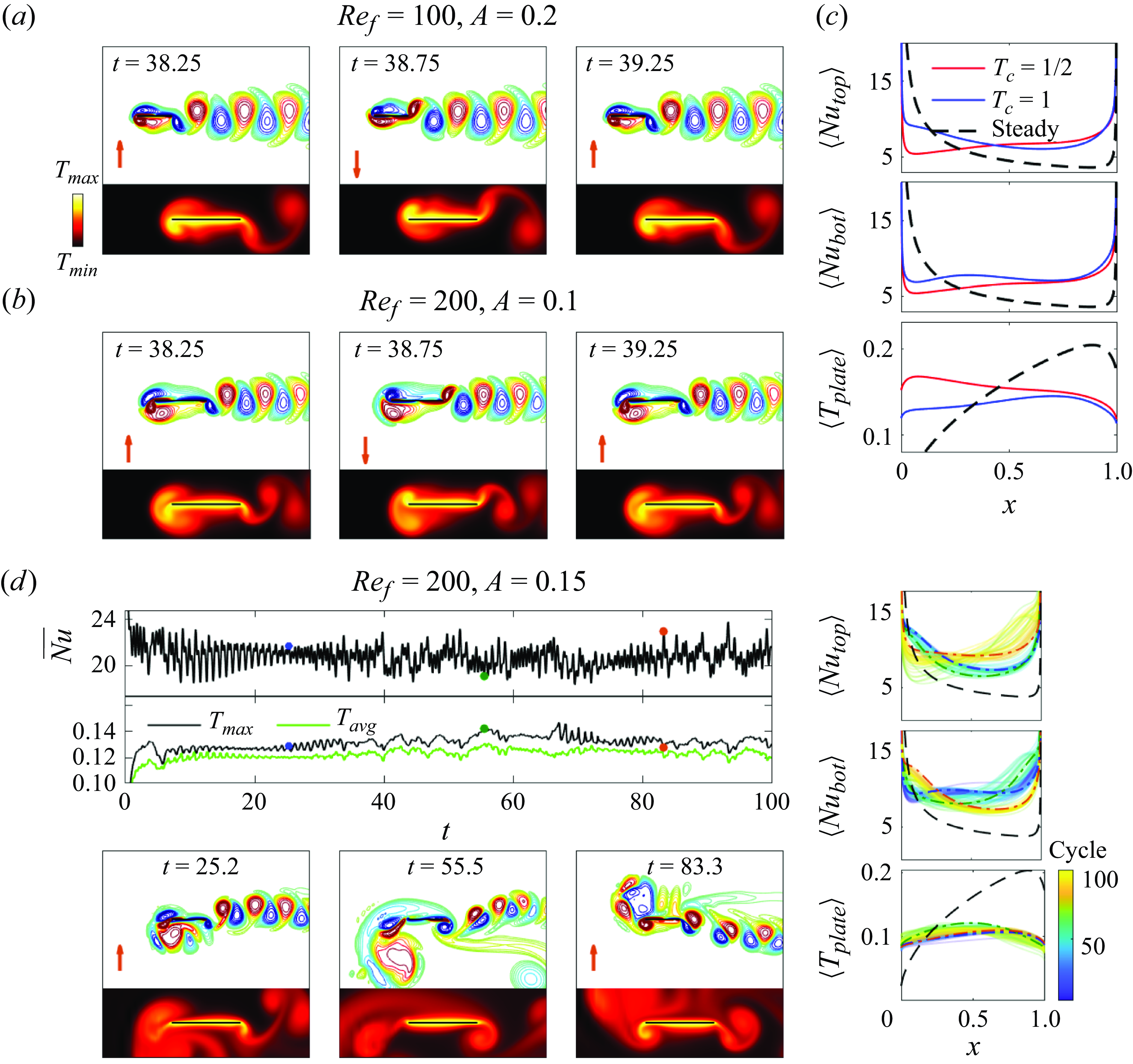
Figure 11. Flows and heat transfer for transverse plate oscillation ( $\alpha = 90^\circ$
) in an in-plane oncoming flow (
$\alpha = 90^\circ$
) in an in-plane oncoming flow ( $\gamma =0^\circ$
). (a) The case with period
$\gamma =0^\circ$
). (a) The case with period $ T_c=1/2$
at
$ T_c=1/2$
at $Re_f=100$
and
$Re_f=100$
and $A=0.2$
, also shown in the supplementary movie 4, accessible here. (b) The case with period
$A=0.2$
, also shown in the supplementary movie 4, accessible here. (b) The case with period $T_c=1$
at
$T_c=1$
at $Re_f=200$
and
$Re_f=200$
and $A=0.1$
, also shown in the supplementary movie 5, accessible here. (c) Comparison of time-averaged local
$A=0.1$
, also shown in the supplementary movie 5, accessible here. (c) Comparison of time-averaged local $Nu$
and plate temperature for (a) and (b). (d) The non-periodic case at
$Nu$
and plate temperature for (a) and (b). (d) The non-periodic case at $Re_f=200$
and
$Re_f=200$
and $A=0.15$
. The three snapshots at the bottom left occur during the 26th, 56th and 84th cycles of oscillation, respectively, and the corresponding cycle-averaged local heat transfer quantities are shown with dash-dotted curves blue, green and orange curves, respectively, in the three rightmost subpanels. This motion is shown in the supplementary movie 6, accessible here. The red arrows in the vorticity snapshots show the instantaneous direction of plate motion. In all cases the black dashed lines show the results for the non-oscillating plate.
$A=0.15$
. The three snapshots at the bottom left occur during the 26th, 56th and 84th cycles of oscillation, respectively, and the corresponding cycle-averaged local heat transfer quantities are shown with dash-dotted curves blue, green and orange curves, respectively, in the three rightmost subpanels. This motion is shown in the supplementary movie 6, accessible here. The red arrows in the vorticity snapshots show the instantaneous direction of plate motion. In all cases the black dashed lines show the results for the non-oscillating plate.
At $A/|\boldsymbol{U}_{\infty }| = 0.3$
, the dynamics instead transitions from periodic to non-periodic as
$A/|\boldsymbol{U}_{\infty }| = 0.3$
, the dynamics instead transitions from periodic to non-periodic as $Re_f$
increases, again with significant improvement of the global heat transfer after the transition. Panel (d) shows examples of the vorticity and temperature fields at
$Re_f$
increases, again with significant improvement of the global heat transfer after the transition. Panel (d) shows examples of the vorticity and temperature fields at $Re_f=200$
, after the transition. Here, vortex grouping occurs in an irregular fashion, and the graphs of
$Re_f=200$
, after the transition. Here, vortex grouping occurs in an irregular fashion, and the graphs of $\overline {Nu}$
,
$\overline {Nu}$
, $T_{{avg}}$
and
$T_{{avg}}$
and $T_{{max}}$
are not close to periodic. We observe three different stages in the vortex dynamics and show one snapshot from each stage. The first snapshot somewhat resembles those in panel (b), with a grouping of positive vortices near the left edge of the bottom wall and a reverse von Kármán vortex street emanating from the right edge. At this instant, blue dashed-dotted lines show the cycle-averaged local heat transfer quantities in the three subpanels on the right side of panel (d). We see some similarities with the blue lines in panel (c). The second snapshot shows the second stage, when the large positive vortex group detaches from the left edge. It continues absorbing positive vortices from the left edge, but is more diffuse than in the previous stage. The local heat transfer quantities for this snapshot are shown by the green dashed-dotted lines in the rightmost subpanels, and are somewhat worse at the middle and left side of the plate than the blue dashed-dotted lines of the first stage. At the right edge the vortex street is more strongly paired as dipoles, and
$T_{{max}}$
are not close to periodic. We observe three different stages in the vortex dynamics and show one snapshot from each stage. The first snapshot somewhat resembles those in panel (b), with a grouping of positive vortices near the left edge of the bottom wall and a reverse von Kármán vortex street emanating from the right edge. At this instant, blue dashed-dotted lines show the cycle-averaged local heat transfer quantities in the three subpanels on the right side of panel (d). We see some similarities with the blue lines in panel (c). The second snapshot shows the second stage, when the large positive vortex group detaches from the left edge. It continues absorbing positive vortices from the left edge, but is more diffuse than in the previous stage. The local heat transfer quantities for this snapshot are shown by the green dashed-dotted lines in the rightmost subpanels, and are somewhat worse at the middle and left side of the plate than the blue dashed-dotted lines of the first stage. At the right edge the vortex street is more strongly paired as dipoles, and $\langle Nu_{{bot}} \rangle$
is improved. The third snapshot approximates a mirror image of the first snapshot, with a region of negative vorticity above the left edge and an array of dipoles shed from the right edge, directed downward. The local heat transfer quantities are shown by the orange dashed-dotted line in the rightmost subpanels. The values of
$\langle Nu_{{bot}} \rangle$
is improved. The third snapshot approximates a mirror image of the first snapshot, with a region of negative vorticity above the left edge and an array of dipoles shed from the right edge, directed downward. The local heat transfer quantities are shown by the orange dashed-dotted line in the rightmost subpanels. The values of $\langle Nu_{{top}}\rangle$
and
$\langle Nu_{{top}}\rangle$
and $\langle Nu_{{bot}} \rangle$
for this snapshot are approximately
$\langle Nu_{{bot}} \rangle$
for this snapshot are approximately $\langle Nu_{{bot}} \rangle$
and
$\langle Nu_{{bot}} \rangle$
and $\langle Nu_{{top}}\rangle$
for the first snapshot (blue dashed-dotted lines), while the
$\langle Nu_{{top}}\rangle$
for the first snapshot (blue dashed-dotted lines), while the $\langle T_{{plate}} \rangle$
distributions are approximately equal, consistent with a mirror-image symmetry of the flows and temperature fields. In these cases and in figures 9 and 10,
$\langle T_{{plate}} \rangle$
distributions are approximately equal, consistent with a mirror-image symmetry of the flows and temperature fields. In these cases and in figures 9 and 10, $\langle Nu \rangle$
has a local minimum near the leading edge on the side facing the large region of merged vortices, and is larger (relative to the steady case, the black dashed line) near the trailing edge. On the other side of the plate,
$\langle Nu \rangle$
has a local minimum near the leading edge on the side facing the large region of merged vortices, and is larger (relative to the steady case, the black dashed line) near the trailing edge. On the other side of the plate, $\langle Nu \rangle$
is instead larger near the leading edge and smaller near the trailing edge. In figure 11(d) and in other non-periodic cases discussed next, vortices merge near one edge into a large cloud over many cycles, then the cloud detaches, and then vortex merging occurs at the other edge. The switching between the edges occurs at somewhat irregular intervals. During these changes in the local heat transfer distribution, the global (spatially averaged) heat transfer does not change much; increases in heat transfer in one region are balanced by decreases in other regions. At lower
$\langle Nu \rangle$
is instead larger near the leading edge and smaller near the trailing edge. In figure 11(d) and in other non-periodic cases discussed next, vortices merge near one edge into a large cloud over many cycles, then the cloud detaches, and then vortex merging occurs at the other edge. The switching between the edges occurs at somewhat irregular intervals. During these changes in the local heat transfer distribution, the global (spatially averaged) heat transfer does not change much; increases in heat transfer in one region are balanced by decreases in other regions. At lower $Re_f$
, 50 and 100, the dynamics is periodic and similar to panel (b). In these two cases
$Re_f$
, 50 and 100, the dynamics is periodic and similar to panel (b). In these two cases $\langle \overline {Nu} \rangle$
values are 28 % and 20 % lower than the non-periodic
$\langle \overline {Nu} \rangle$
values are 28 % and 20 % lower than the non-periodic $Re_f=200$
case, while
$Re_f=200$
case, while $\langle T_{{avg}} \rangle$
values are 37 % and 22 % higher than at
$\langle T_{{avg}} \rangle$
values are 37 % and 22 % higher than at $Re_f=200$
, respectively. The merged vorticity near the leading edge is stronger in the non-periodic case than in the periodic case, and hence more capable of bringing cold fluid towards the plate.
$Re_f=200$
, respectively. The merged vorticity near the leading edge is stronger in the non-periodic case than in the periodic case, and hence more capable of bringing cold fluid towards the plate.
4.2.2. Oblique oncoming flow:
$\gamma =45^\circ$


Figure 12. The cases that optimise global heat transfer ( $\langle \overline {Nu} \rangle$
and
$\langle \overline {Nu} \rangle$
and $\langle T_{{avg}} \rangle$
) at
$\langle T_{{avg}} \rangle$
) at $\gamma =45^\circ$
for
$\gamma =45^\circ$
for $A/|\boldsymbol{U}_{\infty }|=0.2$
(a) and 0.3 (b). The supplementary movies for panel (a) and (b) are named ‘movie 7’ and ‘movie 8’, respectively, and can be found here. In each panel, the four snapshots of the vorticity and temperature field correspond to times marked with red dots on the graphs of
$A/|\boldsymbol{U}_{\infty }|=0.2$
(a) and 0.3 (b). The supplementary movies for panel (a) and (b) are named ‘movie 7’ and ‘movie 8’, respectively, and can be found here. In each panel, the four snapshots of the vorticity and temperature field correspond to times marked with red dots on the graphs of $ \overline {Nu}$
and
$ \overline {Nu}$
and $\langle T_{{max}} \rangle$
, with the red arrows indicating the instantaneous direction of plate motion. The bottom three panels show the cycle-averaged
$\langle T_{{max}} \rangle$
, with the red arrows indicating the instantaneous direction of plate motion. The bottom three panels show the cycle-averaged $\langle Nu \rangle$
of the top and bottom walls for the isothermal plate, and the cycle-averaged
$\langle Nu \rangle$
of the top and bottom walls for the isothermal plate, and the cycle-averaged $\langle T_{{plate}} \rangle$
with fixed heat flux. The first 5 cycles are omitted to avoid transient effects. The black dashed line shows the time-averaged results for the non-oscillating plate in the final periodic state for
$\langle T_{{plate}} \rangle$
with fixed heat flux. The first 5 cycles are omitted to avoid transient effects. The black dashed line shows the time-averaged results for the non-oscillating plate in the final periodic state for $\gamma =45^\circ$
.
$\gamma =45^\circ$
.
The previous section considered the case of the background flow along the plane of the plate, $\gamma = 0^\circ$
. We now consider heat transfer in the same system with
$\gamma = 0^\circ$
. We now consider heat transfer in the same system with $\gamma$
increased to
$\gamma$
increased to $45^\circ$
, an oblique background flow. For any
$45^\circ$
, an oblique background flow. For any $\gamma$
significantly different from
$\gamma$
significantly different from $0^\circ$
, the wake oscillates periodically (for a range of
$0^\circ$
, the wake oscillates periodically (for a range of $Re_U$
near the present value of 100) even for a steady plate, as shown in § 3. When we oscillate the plate also but at a different period, the dynamics can be almost periodic on a longer time scale (i.e. the flow period locks to a multiple of the plate period) or clearly non-periodic, as indicated by the open and filled circles respectively in figure 6 for
$Re_U$
near the present value of 100) even for a steady plate, as shown in § 3. When we oscillate the plate also but at a different period, the dynamics can be almost periodic on a longer time scale (i.e. the flow period locks to a multiple of the plate period) or clearly non-periodic, as indicated by the open and filled circles respectively in figure 6 for $\gamma = 45^\circ$
and 90
$\gamma = 45^\circ$
and 90 $^\circ$
. Almost-periodic cases are the most common at
$^\circ$
. Almost-periodic cases are the most common at $A/|\boldsymbol{U}_{\infty }|=0.2$
, while non-periodic cases are approximately equally common at
$A/|\boldsymbol{U}_{\infty }|=0.2$
, while non-periodic cases are approximately equally common at $A/|\boldsymbol{U}_{\infty }|=0.3$
, and more common with transverse oscillation, when the shed vorticity is stronger. In almost-periodic cases, vortex merging occurs over the same number of plate oscillation cycles and at the same location each time. In non-periodic cases, the locations and dynamics of vortex merging are somewhat irregular. In general, the almost-periodic and non-periodic cases are distinguished by the regularity of the vortex dynamics, but not heat transfer performance. Generally, we see larger heat transfer with stronger vortices, which are also associated with non-periodic flows. But we do not see a direct mechanism by which non-periodicity increases heat transfer relative to almost-periodic flows with vortices of roughly the same strength. If we compare almost-periodic and non-periodic cases with the same
$A/|\boldsymbol{U}_{\infty }|=0.3$
, and more common with transverse oscillation, when the shed vorticity is stronger. In almost-periodic cases, vortex merging occurs over the same number of plate oscillation cycles and at the same location each time. In non-periodic cases, the locations and dynamics of vortex merging are somewhat irregular. In general, the almost-periodic and non-periodic cases are distinguished by the regularity of the vortex dynamics, but not heat transfer performance. Generally, we see larger heat transfer with stronger vortices, which are also associated with non-periodic flows. But we do not see a direct mechanism by which non-periodicity increases heat transfer relative to almost-periodic flows with vortices of roughly the same strength. If we compare almost-periodic and non-periodic cases with the same $A/|\boldsymbol{U}_{\infty }|$
(i.e. the same oscillation velocity), for example,
$A/|\boldsymbol{U}_{\infty }|$
(i.e. the same oscillation velocity), for example, $\gamma =45^\circ$
and
$\gamma =45^\circ$
and $\alpha =120^\circ$
at
$\alpha =120^\circ$
at $A/|\boldsymbol{U}_{\infty }|=0.3$
in figures 6 and 7, we see similar global heat transfer for the open and filled circles.
$A/|\boldsymbol{U}_{\infty }|=0.3$
in figures 6 and 7, we see similar global heat transfer for the open and filled circles.
In figure 12, we show the cases with the best global heat transfer ( $\langle \overline {Nu} \rangle$
) when
$\langle \overline {Nu} \rangle$
) when $\gamma = 45^\circ$
, for
$\gamma = 45^\circ$
, for $A/|\boldsymbol{U}_{\infty }|=0.2$
(panel (a)) and 0.3 (panel (b)). Both occur with transverse oscillation (
$A/|\boldsymbol{U}_{\infty }|=0.2$
(panel (a)) and 0.3 (panel (b)). Both occur with transverse oscillation ( $\alpha =90^\circ$
), which is also optimal at
$\alpha =90^\circ$
), which is also optimal at $\gamma = 0^\circ$
and 90
$\gamma = 0^\circ$
and 90 $^\circ$
. Both optima occur at an intermediate
$^\circ$
. Both optima occur at an intermediate $Re_f$
of 150, but other
$Re_f$
of 150, but other $Re_f$
give similar
$Re_f$
give similar $\langle \overline {Nu} \rangle$
and
$\langle \overline {Nu} \rangle$
and $\langle T_{{avg}}\rangle$
. As indicated by the time series of the global quantities in the first row of each panel, panel (a) is nearly periodic with a period of 17 plate oscillation cycles, while panel (b) is non-periodic. In both cases a dipole sheds alternately from the left and right edge every half-cycle; the stronger vortex of the dipole pair merges with the cloud of previously shed vortices of the same sign and the weaker vortex diffuses. Over many cycles, negative vortices group at the left edge, detach and then positive vortices group at the right edge, detach and the process repeats. (Supplementary movies of these cases, named ‘movie 7’ and ‘movie 8’, can be found here.) During this time, the graphs of the global quantities
$\langle T_{{avg}}\rangle$
. As indicated by the time series of the global quantities in the first row of each panel, panel (a) is nearly periodic with a period of 17 plate oscillation cycles, while panel (b) is non-periodic. In both cases a dipole sheds alternately from the left and right edge every half-cycle; the stronger vortex of the dipole pair merges with the cloud of previously shed vortices of the same sign and the weaker vortex diffuses. Over many cycles, negative vortices group at the left edge, detach and then positive vortices group at the right edge, detach and the process repeats. (Supplementary movies of these cases, named ‘movie 7’ and ‘movie 8’, can be found here.) During this time, the graphs of the global quantities $\overline {\textit{Nu}}$
,
$\overline {\textit{Nu}}$
, $T_{\textit{avg}}$
and
$T_{\textit{avg}}$
and $T_{{max}}$
show oscillations on the time scale of the plate oscillation and on much longer time scales. At the bottom of each panel, the graphs of the local quantities
$T_{{max}}$
show oscillations on the time scale of the plate oscillation and on much longer time scales. At the bottom of each panel, the graphs of the local quantities $\langle Nu_{{top}} \rangle$
,
$\langle Nu_{{top}} \rangle$
, $\langle Nu_{{bot}} \rangle$
and
$\langle Nu_{{bot}} \rangle$
and $\langle T_{{plate}} \rangle$
also oscillate, between distributions with maxima on the left and right alternately for the first and third quantities. These oscillations are correlated with the vortex dynamics shown in the snapshots in the middle of each panel.
$\langle T_{{plate}} \rangle$
also oscillate, between distributions with maxima on the left and right alternately for the first and third quantities. These oscillations are correlated with the vortex dynamics shown in the snapshots in the middle of each panel.
In the first vorticity snapshot of panel (a), a region of negative merged vortices lies above the left edge, which makes $\langle Nu_{{top}} \rangle$
low on the left and high on the right and gives a maximum of
$\langle Nu_{{top}} \rangle$
low on the left and high on the right and gives a maximum of $\langle T_{{plate}} \rangle$
near the left edge. The top subpanel shows
$\langle T_{{plate}} \rangle$
near the left edge. The top subpanel shows $\overline {Nu}$
is generally increasing at this time. In the second vorticity snapshot, a positive vortex group forms and repels the negative vortex group. The maximum of
$\overline {Nu}$
is generally increasing at this time. In the second vorticity snapshot, a positive vortex group forms and repels the negative vortex group. The maximum of $\langle Nu_{{top}} \rangle$
shifts from the right towards the left. The second red dot on the
$\langle Nu_{{top}} \rangle$
shifts from the right towards the left. The second red dot on the $\overline {Nu}$
time series above shows that the global heat transfer reaches a maximum at this time. In the third snapshot, the positive vortex group detaches, while
$\overline {Nu}$
time series above shows that the global heat transfer reaches a maximum at this time. In the third snapshot, the positive vortex group detaches, while $\overline {Nu}$
decreases, reaching a minimum at the time of the fourth snapshot, when the negative vortex group begins to grow again. The graphs of
$\overline {Nu}$
decreases, reaching a minimum at the time of the fourth snapshot, when the negative vortex group begins to grow again. The graphs of $T_{{avg}}$
and
$T_{{avg}}$
and $T_{{max}}$
below show nearly the inverse behaviour for the fixed-flux case, as expected. During this entire cycle
$T_{{max}}$
below show nearly the inverse behaviour for the fixed-flux case, as expected. During this entire cycle $\langle Nu_{{bot}} \rangle$
, which is less influenced by the vortex wake dynamics, has much smaller oscillations about a mean distribution slightly above that of the steady case (black dashed line).
$\langle Nu_{{bot}} \rangle$
, which is less influenced by the vortex wake dynamics, has much smaller oscillations about a mean distribution slightly above that of the steady case (black dashed line).
A few differences are seen in panel (b) ( $A/|\boldsymbol{U}_{\infty }|=0.3$
). The vortex groups form over more oscillation cycles than at
$A/|\boldsymbol{U}_{\infty }|=0.3$
). The vortex groups form over more oscillation cycles than at $A/|\boldsymbol{U}_{\infty }|=0.2$
. In the first snapshot of panel (b), the negative vortex group is more diffuse than in panel (a), with a longer chain of dipoles emanating from the right edge. Meanwhile, the global heat transfer quantities (
$A/|\boldsymbol{U}_{\infty }|=0.2$
. In the first snapshot of panel (b), the negative vortex group is more diffuse than in panel (a), with a longer chain of dipoles emanating from the right edge. Meanwhile, the global heat transfer quantities ( $\overline {Nu}$
,
$\overline {Nu}$
, $T_{{avg}}$
and
$T_{{avg}}$
and $T_{{max}}$
) are nearly steady. In the second snapshot, the positive vortices from the right edge have formed a loose group that repels the negative vortex group, and
$T_{{max}}$
) are nearly steady. In the second snapshot, the positive vortices from the right edge have formed a loose group that repels the negative vortex group, and $\overline {Nu}$
drops to a local minimum. In the third snapshot the positive vortices have formed a more compact group attached to the right edge of the plate, during a long period of increase of
$\overline {Nu}$
drops to a local minimum. In the third snapshot the positive vortices have formed a more compact group attached to the right edge of the plate, during a long period of increase of $\overline {Nu}$
. In the fourth snapshot, the positive vortex group has detached, the negative vortex group is reforming and
$\overline {Nu}$
. In the fourth snapshot, the positive vortex group has detached, the negative vortex group is reforming and $\overline {Nu}$
drops to another local minimum. Meanwhile
$\overline {Nu}$
drops to another local minimum. Meanwhile $\langle Nu_{{top}} \rangle$
,
$\langle Nu_{{top}} \rangle$
, $\langle Nu_{{bot}} \rangle$
and
$\langle Nu_{{bot}} \rangle$
and $\langle T_{{plate}} \rangle$
at the bottom oscillate between distributions similar to those in panel (a), but more erratically and with larger oscillation amplitudes.
$\langle T_{{plate}} \rangle$
at the bottom oscillate between distributions similar to those in panel (a), but more erratically and with larger oscillation amplitudes.
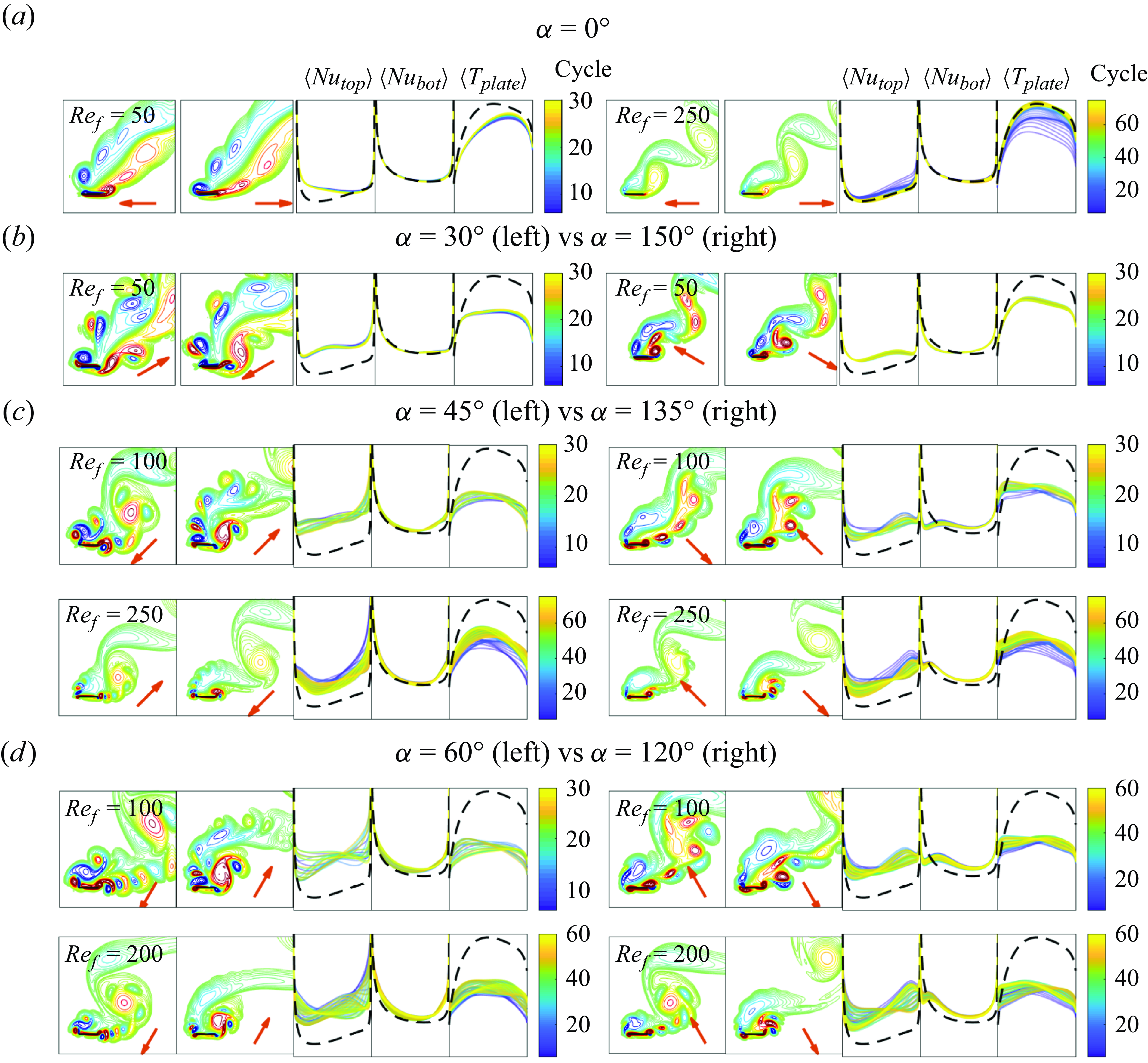
Figure 13. Vorticity fields and cycle-averaged local heat transfer quantities for an oscillating plate in an oblique flow ( $\gamma =45^\circ$
) with
$\gamma =45^\circ$
) with $A/|\boldsymbol{U}_{\infty }| = 0.2$
and
$A/|\boldsymbol{U}_{\infty }| = 0.2$
and $\alpha \neq 90^\circ$
, i.e. oscillation directions other than transverse. The red arrow in each vorticity panel indicates the instantaneous plate velocity direction. Supplementary movies are available at this link for the left case of panel (a) (‘movie 9’), the two cases in panel (b) (‘movie 10’ and ‘movie 11’) and the two cases in panel (c) (‘movie 12’ and ‘movie 13’).
$\alpha \neq 90^\circ$
, i.e. oscillation directions other than transverse. The red arrow in each vorticity panel indicates the instantaneous plate velocity direction. Supplementary movies are available at this link for the left case of panel (a) (‘movie 9’), the two cases in panel (b) (‘movie 10’ and ‘movie 11’) and the two cases in panel (c) (‘movie 12’ and ‘movie 13’).
Figure 13 shows vorticity field snapshots and local heat transfer quantities for oblique flow ( $\gamma =45^\circ$
) and the remaining seven plate oscillation directions, i.e.
$\gamma =45^\circ$
) and the remaining seven plate oscillation directions, i.e. $\alpha \neq 90^\circ$
. We only discuss
$\alpha \neq 90^\circ$
. We only discuss $A/|\boldsymbol{U}_{\infty }|=0.2$
because the phenomena are generally similar at
$A/|\boldsymbol{U}_{\infty }|=0.2$
because the phenomena are generally similar at $A/|\boldsymbol{U}_{\infty }|=0.3$
. In figure 13, we show the variations in vorticity and local heat transfer distributions with a simplified presentation. In each row, two cases are positioned side by side and compared. Two representative snapshots of the vorticity field are selected for each case to indicate the motions of the vortices. We also provide supplementary movies of each case (at the link in the figure caption). The three subpanels to the right of each pair of vorticity fields show the cycle-averaged local quantities. We have removed the axis labels to make the figure compact, but all the subpanels for the cycle-averaged local
$A/|\boldsymbol{U}_{\infty }|=0.3$
. In figure 13, we show the variations in vorticity and local heat transfer distributions with a simplified presentation. In each row, two cases are positioned side by side and compared. Two representative snapshots of the vorticity field are selected for each case to indicate the motions of the vortices. We also provide supplementary movies of each case (at the link in the figure caption). The three subpanels to the right of each pair of vorticity fields show the cycle-averaged local quantities. We have removed the axis labels to make the figure compact, but all the subpanels for the cycle-averaged local $Nu$
and plate temperature share the same y axes, respectively, and the non-oscillating-plate values (the black dashed curve) can be taken as a reference. (Besides the cycle-averaged local quantities, we also show the long-time-averaged local
$Nu$
and plate temperature share the same y axes, respectively, and the non-oscillating-plate values (the black dashed curve) can be taken as a reference. (Besides the cycle-averaged local quantities, we also show the long-time-averaged local $Nu$
in figure 28 in Appendix E.)
$Nu$
in figure 28 in Appendix E.)
The top row (panel (a)) shows in-plane oscillation ( $\alpha =0^\circ$
), for which the largest heat transfer enhancement occurs at
$\alpha =0^\circ$
), for which the largest heat transfer enhancement occurs at $Re_f=50$
(shown on the left side), and mainly on the top side of the plate near the left edge. As
$Re_f=50$
(shown on the left side), and mainly on the top side of the plate near the left edge. As $Re_f$
increases and the amplitude decreases, the enhancement drops. The flow and local heat transfer quantities converge to those of the steady plate, as shown on the right side of panel (a), neglecting the dark blue graphs of the initial transient period before the steady state. With in-plane oscillations, each edge mainly sheds vorticity of a single sign, as for the static plate. Without strong interactions of oppositely signed vorticity, there is relatively weak fluid mixing near the plate.
$Re_f$
increases and the amplitude decreases, the enhancement drops. The flow and local heat transfer quantities converge to those of the steady plate, as shown on the right side of panel (a), neglecting the dark blue graphs of the initial transient period before the steady state. With in-plane oscillations, each edge mainly sheds vorticity of a single sign, as for the static plate. Without strong interactions of oppositely signed vorticity, there is relatively weak fluid mixing near the plate.
The remaining rows, panels (b)–(d), show $\alpha = 30^\circ , 45^\circ $
and
$\alpha = 30^\circ , 45^\circ $
and $60^\circ$
on the left paired with the supplementary angles
$60^\circ$
on the left paired with the supplementary angles $150^\circ , 135^\circ $
and
$150^\circ , 135^\circ $
and $120^\circ$
on the right. For each pair, the transverse velocity component is the same, ranging from smaller (more in plane) at
$120^\circ$
on the right. For each pair, the transverse velocity component is the same, ranging from smaller (more in plane) at $\alpha = 30^\circ$
and
$\alpha = 30^\circ$
and $150^\circ$
(panel (b)) to larger (more transverse) at
$150^\circ$
(panel (b)) to larger (more transverse) at $\alpha = 60^\circ$
and
$\alpha = 60^\circ$
and $120^\circ$
(panel (d)). But the in-plane velocity components are reversed, so the left side (
$120^\circ$
(panel (d)). But the in-plane velocity components are reversed, so the left side ( $\alpha \lt 90^\circ$
) oscillates more along the oncoming flow direction while the right side (
$\alpha \lt 90^\circ$
) oscillates more along the oncoming flow direction while the right side ( $\alpha \gt 90^\circ$
) oscillates more across it, as seen from the plate velocity vectors (red arrows) in each panel. In figure 7 we saw that oscillating along the flow is better, i.e. within each pair
$\alpha \gt 90^\circ$
) oscillates more across it, as seen from the plate velocity vectors (red arrows) in each panel. In figure 7 we saw that oscillating along the flow is better, i.e. within each pair $\alpha \lt 90^\circ$
outperforms
$\alpha \lt 90^\circ$
outperforms $\alpha \gt 90^\circ$
, and the difference between the two becomes smaller as
$\alpha \gt 90^\circ$
, and the difference between the two becomes smaller as $Re_f$
increases. This is also seen in the local heat transfer graphs of figure 13, for which
$Re_f$
increases. This is also seen in the local heat transfer graphs of figure 13, for which $\langle Nu_{{top/bot}} \rangle$
is generally higher and
$\langle Nu_{{top/bot}} \rangle$
is generally higher and $\langle T_{{plate}} \rangle$
is lower relative to the steady reference case (black dashed) on the left side, oscillating along the flow.
$\langle T_{{plate}} \rangle$
is lower relative to the steady reference case (black dashed) on the left side, oscillating along the flow.
Previously, we mentioned that stronger vorticity is found near the plate for $\alpha \lt 90^\circ$
than
$\alpha \lt 90^\circ$
than $\alpha \gt 90^\circ$
(as shown in figure 25 in Appendix D), which might be a short explanation for the better heat transfer achieved with
$\alpha \gt 90^\circ$
(as shown in figure 25 in Appendix D), which might be a short explanation for the better heat transfer achieved with $\alpha \lt 90^\circ$
. We now give a more detailed explanation by showing the differences in vortex dynamics for
$\alpha \lt 90^\circ$
. We now give a more detailed explanation by showing the differences in vortex dynamics for $\alpha \lt 90^\circ$
and
$\alpha \lt 90^\circ$
and $\alpha \gt 90^\circ$
. With
$\alpha \gt 90^\circ$
. With $A/|\boldsymbol{U}_{\infty }|$
= 0.2, the ratio of the maximum plate velocity to the oncoming flow velocity is
$A/|\boldsymbol{U}_{\infty }|$
= 0.2, the ratio of the maximum plate velocity to the oncoming flow velocity is $2\pi \cdot 0.2 = 1.26$
, so the plate oscillation is strong enough to reverse the oncoming flow velocity. This occurs for
$2\pi \cdot 0.2 = 1.26$
, so the plate oscillation is strong enough to reverse the oncoming flow velocity. This occurs for $\alpha = 45^\circ$
, when the plate oscillates along the flow, and at nearby values, i.e. over most of the range
$\alpha = 45^\circ$
, when the plate oscillates along the flow, and at nearby values, i.e. over most of the range $0^\circ \lt \alpha \lt 90^\circ$
. In this case, oppositely signed vortices are shed from each edge on each cycle, and they have relatively strong interactions and mix the fluid close to the plate, as can be seen in the vorticity snapshots on the left sides of panels (b)–(d). When
$0^\circ \lt \alpha \lt 90^\circ$
. In this case, oppositely signed vortices are shed from each edge on each cycle, and they have relatively strong interactions and mix the fluid close to the plate, as can be seen in the vorticity snapshots on the left sides of panels (b)–(d). When $\alpha = 135^\circ$
, the plate oscillates across the flow, and there is always a positive flow component in the oncoming flow direction. The same is true over most of the range
$\alpha = 135^\circ$
, the plate oscillates across the flow, and there is always a positive flow component in the oncoming flow direction. The same is true over most of the range $90^\circ \lt \alpha \lt 180^\circ$
. In this case, the vorticity shed from each edge is predominantly (but not completely) single signed, similarly to the in-plane oscillation of panel (a). Here there are weaker interactions between the vortices near the plate, before they are advected away by the oncoming flow, as seen in the vorticity snapshots on the right sides of panels (b)–(d). These differences may underlie some of the common features of the local heat transfer quantities on the left and right. For example, the right subpanels but not the left subpanels show a dip in
$90^\circ \lt \alpha \lt 180^\circ$
. In this case, the vorticity shed from each edge is predominantly (but not completely) single signed, similarly to the in-plane oscillation of panel (a). Here there are weaker interactions between the vortices near the plate, before they are advected away by the oncoming flow, as seen in the vorticity snapshots on the right sides of panels (b)–(d). These differences may underlie some of the common features of the local heat transfer quantities on the left and right. For example, the right subpanels but not the left subpanels show a dip in $\langle Nu_{{bot}} \rangle$
, and a rise in
$\langle Nu_{{bot}} \rangle$
, and a rise in $\langle T_{{plate}} \rangle$
, at the left edge relative to the steady graph (black dashed line). The difference between the two cases diminishes as
$\langle T_{{plate}} \rangle$
, at the left edge relative to the steady graph (black dashed line). The difference between the two cases diminishes as $Re_f$
increases, because the vorticity fields become more similar. This is seen in the second rows of panels (c) and (d), where the vorticity snapshots are more similar on the left and right sides than in the first rows, at lower
$Re_f$
increases, because the vorticity fields become more similar. This is seen in the second rows of panels (c) and (d), where the vorticity snapshots are more similar on the left and right sides than in the first rows, at lower $Re_f$
.
$Re_f$
.
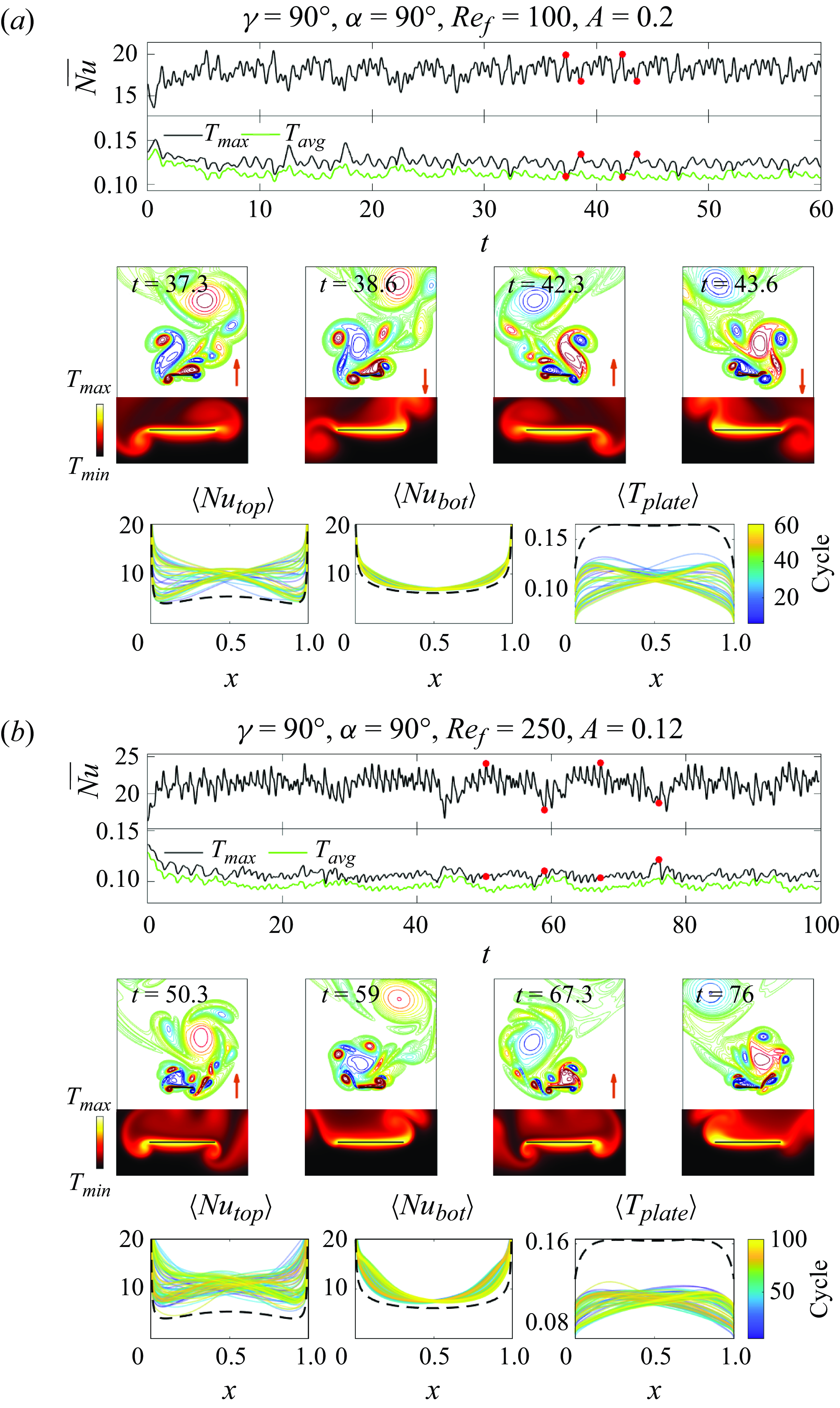
Figure 14. The cases that optimise global heat transfer ( $\langle \overline {Nu} \rangle$
and
$\langle \overline {Nu} \rangle$
and $\langle T_{{avg}} \rangle$
) at
$\langle T_{{avg}} \rangle$
) at $\gamma =90^\circ$
for
$\gamma =90^\circ$
for $A/|\boldsymbol{U}_{\infty }|=0.2$
(a) and 0.3 (b), with supplementary movies named ‘14‘ and ‘15’, respectively, linked here. In each panel, the four snapshots of the vorticity and temperature field correspond to times marked with red dots on the graphs of
$A/|\boldsymbol{U}_{\infty }|=0.2$
(a) and 0.3 (b), with supplementary movies named ‘14‘ and ‘15’, respectively, linked here. In each panel, the four snapshots of the vorticity and temperature field correspond to times marked with red dots on the graphs of $ \overline {Nu}$
and
$ \overline {Nu}$
and $\langle T_{{max}} \rangle$
, with the red arrows indicating the instantaneous direction of plate motion. The bottom three panels show the cycle-averaged
$\langle T_{{max}} \rangle$
, with the red arrows indicating the instantaneous direction of plate motion. The bottom three panels show the cycle-averaged $\langle Nu \rangle$
of the top and bottom walls for the isothermal plate, and the cycle-averaged
$\langle Nu \rangle$
of the top and bottom walls for the isothermal plate, and the cycle-averaged $\langle T_{{plate}} \rangle$
with fixed heat flux. The first 5 cycles are omitted to avoid transient effects. The black dashed line shows the time-averaged results for the non-oscillating plate in the final periodic state for
$\langle T_{{plate}} \rangle$
with fixed heat flux. The first 5 cycles are omitted to avoid transient effects. The black dashed line shows the time-averaged results for the non-oscillating plate in the final periodic state for $\gamma =90^\circ$
, after the symmetry breaking.
$\gamma =90^\circ$
, after the symmetry breaking.
4.2.3. Transverse oncoming flow:
$\gamma =90^\circ$

Having discussed in-plane and oblique oncoming flows, $\gamma =0^\circ$
and
$\gamma =0^\circ$
and $45^\circ$
, we now consider transverse oncoming flow,
$45^\circ$
, we now consider transverse oncoming flow, $\gamma =90^\circ$
. Due to symmetry, we can restrict ourselves to
$\gamma =90^\circ$
. Due to symmetry, we can restrict ourselves to $0^\circ \leqslant \alpha \leqslant 90^\circ$
. As before, the best global heat transfer occurs with transverse plate oscillations (
$0^\circ \leqslant \alpha \leqslant 90^\circ$
. As before, the best global heat transfer occurs with transverse plate oscillations ( $\alpha =90^\circ$
). At these particular
$\alpha =90^\circ$
). At these particular $\alpha$
and
$\alpha$
and $\gamma$
, as for the steady plate at
$\gamma$
, as for the steady plate at $\gamma =90^\circ$
, a uniform initial oncoming flow with small asymmetric perturbations reaches the asymmetric steady state slowly, after
$\gamma =90^\circ$
, a uniform initial oncoming flow with small asymmetric perturbations reaches the asymmetric steady state slowly, after ${\approx}300$
time units. To reach the steady state faster, we instead initialise the flow and temperature fields to be those at
${\approx}300$
time units. To reach the steady state faster, we instead initialise the flow and temperature fields to be those at $t=400$
for the steady plate with
$t=400$
for the steady plate with $\gamma =90^\circ$
, similar to the cases shown at the latest times in figure 5, which have a von Kármán vortex wake.
$\gamma =90^\circ$
, similar to the cases shown at the latest times in figure 5, which have a von Kármán vortex wake.
The optimal flows for heat transfer at $A/|\boldsymbol{U}_{\infty }|=0.2$
and 0.3 are shown in figures 14(a) and 14(b), respectively, using a layout similar to figure 12, with links to corresponding movies in the caption. With the combination of a plate oscillation frequency and the bluff-body wake shedding frequency, the vortex dynamics and resulting heat transfer for
$A/|\boldsymbol{U}_{\infty }|=0.2$
and 0.3 are shown in figures 14(a) and 14(b), respectively, using a layout similar to figure 12, with links to corresponding movies in the caption. With the combination of a plate oscillation frequency and the bluff-body wake shedding frequency, the vortex dynamics and resulting heat transfer for $\gamma =90^\circ$
are generally similar to those for
$\gamma =90^\circ$
are generally similar to those for $\gamma =45^\circ$
in a few ways. First, in both cases complex vortex-shedding patterns occur in the wake, and greatly enhance heat transfer on the top of the plate (the side facing the wake). Second, shed vortices merge into large regions of single-signed vorticity over many oscillation periods, and then detach, alternately at one edge and then the other. Third, in most cases at
$\gamma =45^\circ$
in a few ways. First, in both cases complex vortex-shedding patterns occur in the wake, and greatly enhance heat transfer on the top of the plate (the side facing the wake). Second, shed vortices merge into large regions of single-signed vorticity over many oscillation periods, and then detach, alternately at one edge and then the other. Third, in most cases at $A/|\boldsymbol{U}_{\infty }|=0.2$
the vortex dynamics is close to periodic and locked to a multiple of the plate oscillation period (10 in panel (a)), while at
$A/|\boldsymbol{U}_{\infty }|=0.2$
the vortex dynamics is close to periodic and locked to a multiple of the plate oscillation period (10 in panel (a)), while at $A/|\boldsymbol{U}_{\infty }|=0.3$
more cases are non-periodic, particularly near
$A/|\boldsymbol{U}_{\infty }|=0.3$
more cases are non-periodic, particularly near $\alpha = 90^\circ$
. One difference is the bilateral symmetry of the
$\alpha = 90^\circ$
. One difference is the bilateral symmetry of the $\gamma =\alpha = 90^\circ$
cases, e.g. in figure 14, so that the positive and negative vortex groups are essentially mirror images in the two leftmost and rightmost snapshots of the periodic case in panel (a), and almost mirror images in the non-periodic case of panel (b). A corresponding left-right symmetry is seen in the ensemble of cycle-averaged
$\gamma =\alpha = 90^\circ$
cases, e.g. in figure 14, so that the positive and negative vortex groups are essentially mirror images in the two leftmost and rightmost snapshots of the periodic case in panel (a), and almost mirror images in the non-periodic case of panel (b). A corresponding left-right symmetry is seen in the ensemble of cycle-averaged $\langle Nu_{{top}} \rangle$
,
$\langle Nu_{{top}} \rangle$
, $\langle Nu_{{bot}} \rangle$
and
$\langle Nu_{{bot}} \rangle$
and $\langle T_{{plate}} \rangle$
distributions in panel (a), and to a lesser extent in panel (b). Key features of the graphs of the global heat transfer quantities are correlated with events in the vortex dynamics, similarly to
$\langle T_{{plate}} \rangle$
distributions in panel (a), and to a lesser extent in panel (b). Key features of the graphs of the global heat transfer quantities are correlated with events in the vortex dynamics, similarly to $\gamma = 45^\circ$
. Troughs in
$\gamma = 45^\circ$
. Troughs in $\overline {Nu}$
and peaks in
$\overline {Nu}$
and peaks in $T_{{avg}}$
and
$T_{{avg}}$
and $T_{{max}}$
in panels (a) and (b) occur when a vortex group detaches from one edge and starts to form at the other edge, as shown in the second and fourth snapshots of each panel. During the process of vortex merging, the global heat transfer quantities first increase and then oscillate about fairly constant levels, as occurs during the first and third snapshot of panel (b).
$T_{{max}}$
in panels (a) and (b) occur when a vortex group detaches from one edge and starts to form at the other edge, as shown in the second and fourth snapshots of each panel. During the process of vortex merging, the global heat transfer quantities first increase and then oscillate about fairly constant levels, as occurs during the first and third snapshot of panel (b).
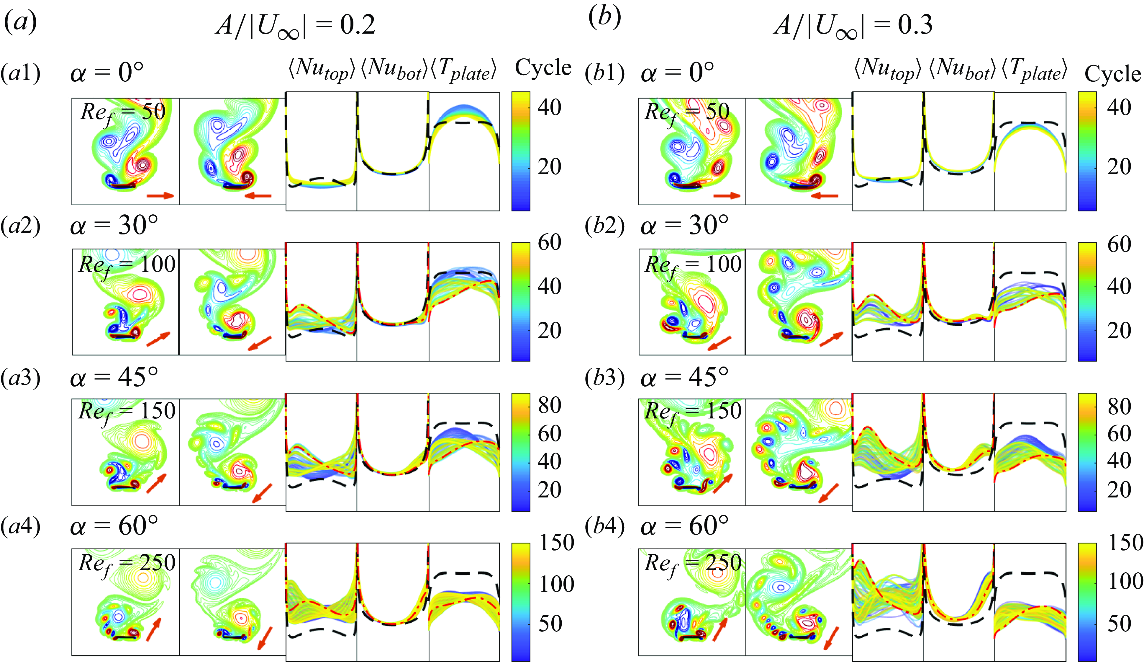
Figure 15. Vorticity fields and cycle-averaged local heat transfer quantities for an oscillating plate in a transverse flow ( $\gamma =90^\circ$
) with
$\gamma =90^\circ$
) with $A/|\boldsymbol{U}_{\infty }| = 0.2$
(a) and 0.3 (b) and
$A/|\boldsymbol{U}_{\infty }| = 0.2$
(a) and 0.3 (b) and $\alpha \neq 90^\circ$
, i.e. oscillation directions other than transverse. The red arrow in each vorticity panel indicates the instantaneous plate velocity direction. The red dash-dotted curves show instantaneous distributions of cycle-averaged local heat transfer quantities that are discussed in the main text. Supplementary movies named ‘movie 16’ and ‘movie 17’ are available here for panels (
$\alpha \neq 90^\circ$
, i.e. oscillation directions other than transverse. The red arrow in each vorticity panel indicates the instantaneous plate velocity direction. The red dash-dotted curves show instantaneous distributions of cycle-averaged local heat transfer quantities that are discussed in the main text. Supplementary movies named ‘movie 16’ and ‘movie 17’ are available here for panels ( $a1$
) and (
$a1$
) and ( $b3$
), respectively.
$b3$
), respectively.
Examples of flows and heat transfer quantities for the other plate oscillation directions are shown in figure 15, for $A/|\boldsymbol{U}_{\infty }|=0.2$
(panel (a)) and 0.3 (panel (b)). For each case shown, the first vorticity snapshot shows the negative vortex/vortex group at the left edge, while the second vorticity snapshot shows the positive vortex/vortex group at the right edge. To the right of the two snapshots, the cycle-averaged local quantities are shown with the same
$A/|\boldsymbol{U}_{\infty }|=0.2$
(panel (a)) and 0.3 (panel (b)). For each case shown, the first vorticity snapshot shows the negative vortex/vortex group at the left edge, while the second vorticity snapshot shows the positive vortex/vortex group at the right edge. To the right of the two snapshots, the cycle-averaged local quantities are shown with the same $y$
-axis scales. Similar to figure 13, the axis labels are removed to make the figure compact but the result for the non-oscillating plate (black dashed curve) can be taken as a reference. The second vorticity snapshots in the last three rows show typical vorticity patterns for
$y$
-axis scales. Similar to figure 13, the axis labels are removed to make the figure compact but the result for the non-oscillating plate (black dashed curve) can be taken as a reference. The second vorticity snapshots in the last three rows show typical vorticity patterns for $\gamma =90^\circ$
, with the corresponding distributions of the cycle-averaged local quantities highlighted with red dash-dotted curves. The caption lists links to two supplementary movies that show the dynamics of the vortices and local heat transfer distributions. As a supplement, the time-averaged local Nusselt number is shown in figure 29 in Appendix E.
$\gamma =90^\circ$
, with the corresponding distributions of the cycle-averaged local quantities highlighted with red dash-dotted curves. The caption lists links to two supplementary movies that show the dynamics of the vortices and local heat transfer distributions. As a supplement, the time-averaged local Nusselt number is shown in figure 29 in Appendix E.
Subpanels (a1) and (b1) show the in-plane-oscillation case ( $\alpha =0^\circ$
). As occurred with
$\alpha =0^\circ$
). As occurred with $\gamma = 45^\circ$
, the most noticeable heat transfer enhancement relative to the steady case occurs at this value of
$\gamma = 45^\circ$
, the most noticeable heat transfer enhancement relative to the steady case occurs at this value of $Re_f$
, the lowest (see figure 7). The graphs of
$Re_f$
, the lowest (see figure 7). The graphs of $\langle Nu_{{top}} \rangle$
and
$\langle Nu_{{top}} \rangle$
and $\langle T_{{plate}} \rangle$
show that the local heat transfer is enhanced mainly at the edges and less enhanced or even worsened in the middle. The overall enhancement in both subpanels (a1) and (b1) is very limited. In these subpanels the cycle-averaged local heat transfer quantities have a left–right symmetry that is broken for the
$\langle T_{{plate}} \rangle$
show that the local heat transfer is enhanced mainly at the edges and less enhanced or even worsened in the middle. The overall enhancement in both subpanels (a1) and (b1) is very limited. In these subpanels the cycle-averaged local heat transfer quantities have a left–right symmetry that is broken for the $\alpha$
in the following subpanels. Here, we have vortex groupings at both edges, with the positive vortex group (above the right edge) more prominent. It usually lasts longer, is more compact and intense and is closer to the top wall than the negative vortex group. In subpanels (
$\alpha$
in the following subpanels. Here, we have vortex groupings at both edges, with the positive vortex group (above the right edge) more prominent. It usually lasts longer, is more compact and intense and is closer to the top wall than the negative vortex group. In subpanels ( $a2$
), (
$a2$
), ( $b2$
), (
$b2$
), ( $a3$
) and (
$a3$
) and ( $b3$
), the negative vortex group is partially or fully separated into individual vortices, while the positive vortex group is a single compact region at the right edge. When the positive vortex group grows to a certain size, it is repelled by the negative vortex group and detaches from the plate. At higher
$b3$
), the negative vortex group is partially or fully separated into individual vortices, while the positive vortex group is a single compact region at the right edge. When the positive vortex group grows to a certain size, it is repelled by the negative vortex group and detaches from the plate. At higher $Re_f$
, the negative vortex group also forms into a compact group attached to the plate, as shown in subpanels (
$Re_f$
, the negative vortex group also forms into a compact group attached to the plate, as shown in subpanels ( $a4$
) and (
$a4$
) and ( $b4$
), but the positive vortex group still lasts longer. The second snapshots in the last three rows of subpanels show an instant when the positive vortex group is detaching from the plate and dipoles have been shed from the left edge. At these times,
$b4$
), but the positive vortex group still lasts longer. The second snapshots in the last three rows of subpanels show an instant when the positive vortex group is detaching from the plate and dipoles have been shed from the left edge. At these times, $\langle Nu_{{top}} \rangle$
has a local maximum near the left edge and a local minimum near the right edge, with the inverse pattern in
$\langle Nu_{{top}} \rangle$
has a local maximum near the left edge and a local minimum near the right edge, with the inverse pattern in $\langle T_{{plate}} \rangle$
, as shown by the red dash-dotted lines.
$\langle T_{{plate}} \rangle$
, as shown by the red dash-dotted lines.
5. Input power
In the previous sections we studied the heat transfer of oscillating plates without considering what drives the oscillation and what input power may be required. Both natural (e.g. plants) and human-made structures can passively vibrate in ambient air and water flows, in which case no additional power source is required to produce the flow (Dowell & Hall Reference Dowell and Hall2001; Heil & Hazel Reference Heil and Hazel2011; Leontini et al. Reference Leontini, Lo Jacono and Thompson2013; Mavroyiakoumou & Alben Reference Mavroyiakoumou and Alben2021, Reference Mavroyiakoumou and Alben2022; Alben Reference Alben2022; Wang & Christov Reference Wang and Christov2022). Many previous studies have examined the benefits of passive fluid–structure interaction for heat transfer specifically (Kim & Choi Reference Kim and Choi2004; Soti, Bhardwaj & Sheridan Reference Soti, Bhardwaj and Sheridan2015; Glezer, Mittal & Alben Reference Glezer, Mittal and Alben2016; Lee et al. Reference Lee, Park, Kim, Ryu and Sung2017; Gosselin Reference Gosselin2019; Solano, Ordonez & Shoele Reference Solano, Ordonez and Shoele2020; Kumar et al. Reference Kumar, Garg, Sharma and Bhardwaj2020).
In other situations, power is needed to oscillate the plate but the ambient flow is free. Flapping plates are a model for the wings or fins of flying and swimming animals in ambient flows (Dabiri Reference Dabiri2009). Under ‘free locomotion’, the organism reaches a steady state with non-zero forward velocity in a quiescent flow, in which case the ambient flow is simply the negative of the forward velocity of the organism (Alben & Shelley Reference Alben and Shelley2005; Alben et al. Reference Alben, Witt, Baker, Anderson and Lauder2012; Tytell et al. Reference Tytell, Leftwich, Hsu, Griffith, Cohen, Smits, Hamlet and Fauci2016; Hoover et al. Reference Hoover, Cortez, Tytell and Fauci2018; Godoy-Diana et al. Reference Godoy-Diana, Vacher, Raspa and Thiria2019; Alben Reference Alben2021b ). Other examples are energy-harvesting applications in which flapping bodies are used to harvest energy from the ambient flow (Zhu & Peng Reference Zhu and Peng2009; Zhu Reference Zhu2011).
One may also consider the power needed to oscillate the plate and drive the oncoming flow. Recent works have calculated the flows that maximise heat transfer for a given total power needed to drive the flow, for flows through channels (Alben Reference Alben2017a ; Alben, Prabala & Godek Reference Alben, Prabala and Godek2024), between parallel heated walls (Hassanzadeh, Chini & Doering Reference Hassanzadeh, Chini and Doering2014; Tobasco & Doering Reference Tobasco and Doering2017; Motoki et al. Reference Motoki, Kawahara and Shimizu2018a ,Reference Motoki, Kawahara and Shimizu b ; Souza, Tobasco & Doering Reference Souza, Tobasco and Doering2020; Kumar 2022; Alben Reference Alben2023) and in more general geometries (Alben Reference Alben2017b ).
Here, we will consider the input power in two situations. In the first, the oncoming flow is freely available from the environment but power is needed to oscillate the plate. In the second situation, power is needed both to drive the oncoming flow past the moving plate and to oscillate the plate. In the previous sections we found that the best global heat transfer occurs with transverse oscillation ( $\alpha =90^\circ$
). However, more power may be required to sustain transverse oscillation because it displaces more fluid than other oscillation directions. Varying the oncoming flow direction from transverse to in plane has a similar effect on the power needed to drive the flow.
$\alpha =90^\circ$
). However, more power may be required to sustain transverse oscillation because it displaces more fluid than other oscillation directions. Varying the oncoming flow direction from transverse to in plane has a similar effect on the power needed to drive the flow.
First, we express the input power needed to oscillate the plate. The horizontal force exerted on the plate by the fluid is due to viscous shear stress on the two sides of the plate
 \begin{equation} F_x(t) = \displaystyle \frac {1}{Re_f}\int _0^1 [ \partial _y u(x, 0, t)]_-^+ \, \textrm{d} x, \end{equation}
where the bracket notation denotes the jump along the plate, the value on the top minus the value on the bottom. The vertical force on the plate is due to the pressure difference between the two sides
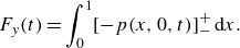 \begin{equation} F_y(t) = \displaystyle \int _0^1 [ -p(x, 0, t)]_-^+ \, \textrm{d} x. \end{equation}
The power needed to move the plate is the product of the force the plate exerts on the fluid ( $-F_x,-F_y$
) with the sinusoidal velocity given in equation (2.1), i.e.
$-F_x,-F_y$
) with the sinusoidal velocity given in equation (2.1), i.e.
 \begin{equation} P_{{body}} (t) = -(F_x(t)\times U_b(t) + F_y(t) \times V_b(t)), \quad \tilde {P}_{{body}} = Re_f^3P_{{body}}. \end{equation}
Equation (5.3) is the total input power required if the oncoming flow is freely available. In (5.3) we rescale the power by multiplying it by $Re_f^3$
. The rescaled power corresponds to using
$Re_f^3$
. The rescaled power corresponds to using $\nu ^\star/\ell ^\star$
as the characteristic velocity scale instead of
$\nu ^\star/\ell ^\star$
as the characteristic velocity scale instead of $f^\star\ell ^\star$
. Then the power non-dimensionalisation does not depend on frequency, which allows us to compare results with different frequencies (i.e. different
$f^\star\ell ^\star$
. Then the power non-dimensionalisation does not depend on frequency, which allows us to compare results with different frequencies (i.e. different $Re_f$
).
$Re_f$
).
To consider the power required for the oncoming flow, we can write the energy balance for a fixed rectangular region $R$
containing the oscillating plate (Kundu, Cohen & Dowling Reference Kundu, Cohen and Dowling2016)
$R$
containing the oscillating plate (Kundu, Cohen & Dowling Reference Kundu, Cohen and Dowling2016)
 \begin{align} \frac {d}{{\textrm d}t}\iint _R \frac {1}{2} u_i^2 {\textrm d}A = -\oint _{\partial R + {plate}} \frac {1}{2}u_i^2 u_j n_j {\textrm d}s + \oint _{\partial R + {plate}} u_i \tau _{ij} n_j {\textrm d}s - \iint _R \frac {2}{Re_f}e_{ij}^2 {\textrm d}A. \end{align}
We have used tensor index notation to express the terms more easily. The equation says that the rate of change of fluid kinetic energy in the rectangle equals the sum of three terms: the net inward flux of kinetic energy ( $n_j$
is the outward unit normal vector), the rate of work done on the fluid in
$n_j$
is the outward unit normal vector), the rate of work done on the fluid in $R$
by pressure and viscous stresses from the oscillating plate and at the outer boundary of
$R$
by pressure and viscous stresses from the oscillating plate and at the outer boundary of $R$
(
$R$
( $\tau _{ij}$
is the stress tensor) and the rate of viscous dissipation in the rectangle (
$\tau _{ij}$
is the stress tensor) and the rate of viscous dissipation in the rectangle ( $e_{ij}$
is the rate-of-strain tensor). When we take a long-time-average, the left-hand side is zero. Hence, the average power dissipated is supplied by the stresses at the plate and outer boundary and by kinetic energy flux at the outer boundary. In heat exchangers, the dominant contribution from the outer boundary is from the pressure stresses there, and is called the `pumping power’ (Rathore & Kapuno Reference Rathore and Kapuno2010).
$e_{ij}$
is the rate-of-strain tensor). When we take a long-time-average, the left-hand side is zero. Hence, the average power dissipated is supplied by the stresses at the plate and outer boundary and by kinetic energy flux at the outer boundary. In heat exchangers, the dominant contribution from the outer boundary is from the pressure stresses there, and is called the `pumping power’ (Rathore & Kapuno Reference Rathore and Kapuno2010).
We define the average input power required for the entire flow, the oncoming flow plus that induced by the oscillating plate, to be the time average of all the terms at the plate and at the outer boundary in (5.4), in the limit that the outer boundary $\partial R$
tends to infinite distance from the body. By (5.4), the sum of all the terms at the plate and outer boundary equals the average viscous power dissipation rate. To calculate this term, we consider the flow in the frame that is at rest in the far field by adding
$\partial R$
tends to infinite distance from the body. By (5.4), the sum of all the terms at the plate and outer boundary equals the average viscous power dissipation rate. To calculate this term, we consider the flow in the frame that is at rest in the far field by adding $-\boldsymbol{U}_{\infty }$
to the fluid velocity. In this frame the body moves upstream while it oscillates and has velocity
$-\boldsymbol{U}_{\infty }$
to the fluid velocity. In this frame the body moves upstream while it oscillates and has velocity $\boldsymbol{U}_{b}-\boldsymbol{U}_{\infty }$
. For this flow,
$\boldsymbol{U}_{b}-\boldsymbol{U}_{\infty }$
. For this flow, $e_{ij}$
is the same as before. As the boundary of
$e_{ij}$
is the same as before. As the boundary of $R$
tends to infinite distance from the body, all the work is done at the body surface, because then there is no other source of energy input. In effect we have replaced the power to drive the flow past the body with the power to move the body upstream into a quiescent flow.
$R$
tends to infinite distance from the body, all the work is done at the body surface, because then there is no other source of energy input. In effect we have replaced the power to drive the flow past the body with the power to move the body upstream into a quiescent flow.
Thus, the average total power required for the plate oscillation plus the oncoming flow is
 \begin{equation} \langle P_{{total}}(t) \rangle = -F_x(t)\times (U_{b}(t)-U_{\infty }) -F_y(t) \times (V_{b}(t)-V_{\infty }), \!\!\quad \langle \tilde {P}_{{total}} \rangle = Re_f^3\langle P_{{total}} \rangle , \end{equation}
which is (5.3) but with the body velocity in the frame where it moves upstream into a quiescent far-field flow. In (5.5), as in (5.3), we rescale the power by $Re_f^3$
to remove the frequency dependence of the non-dimensionalisation.
$Re_f^3$
to remove the frequency dependence of the non-dimensionalisation.
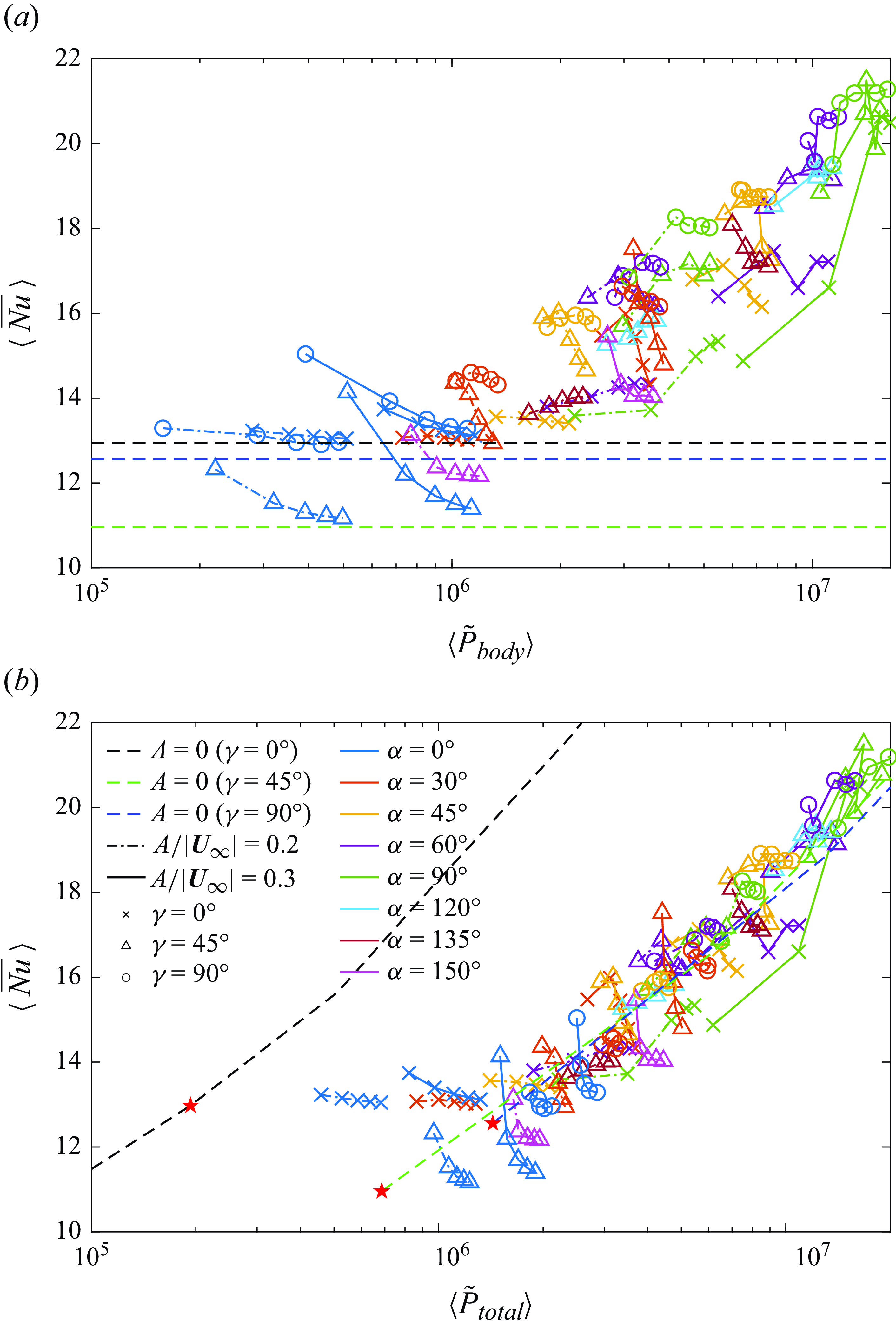
Figure 16. The value of $\langle \overline {Nu} \rangle$
versus (a) the time-averaged power needed to oscillate the plate, and (b) the time-averaged total power including the power needed to drive the oncoming uniform flow. The three horizontal dashed lines in panel (a) show
$\langle \overline {Nu} \rangle$
versus (a) the time-averaged power needed to oscillate the plate, and (b) the time-averaged total power including the power needed to drive the oncoming uniform flow. The three horizontal dashed lines in panel (a) show $\langle \overline {Nu} \rangle$
at
$\langle \overline {Nu} \rangle$
at $Re_U = 100$
for the non-oscillating plates, for which
$Re_U = 100$
for the non-oscillating plates, for which $\langle \tilde {P}_{{body}} \rangle$
= 0. In panel (b) the data for the non-oscillating plates correspond to
$\langle \tilde {P}_{{body}} \rangle$
= 0. In panel (b) the data for the non-oscillating plates correspond to $Re_U$
ranging from 100 to 500 for the green and blue dashed lines, and also include
$Re_U$
ranging from 100 to 500 for the green and blue dashed lines, and also include $Re_U$
below 100 for the black dashed line. The values with
$Re_U$
below 100 for the black dashed line. The values with $Re_U = 100$
are marked with red stars.
$Re_U = 100$
are marked with red stars.
In figure 16 we plot $\langle \overline {Nu} \rangle$
versus
$\langle \overline {Nu} \rangle$
versus $\langle \tilde {P}_{{body}} \rangle$
(panel (a)) and
$\langle \tilde {P}_{{body}} \rangle$
(panel (a)) and $\langle \tilde {P}_{{total}} \rangle$
(panel (b)) for all of the isothermal-plate cases. We compute
$\langle \tilde {P}_{{total}} \rangle$
(panel (b)) for all of the isothermal-plate cases. We compute $\langle \tilde {P}_{{body}} \rangle$
and
$\langle \tilde {P}_{{body}} \rangle$
and $\langle \tilde {P}_{{total}} \rangle$
using the same time spans as for
$\langle \tilde {P}_{{total}} \rangle$
using the same time spans as for $\langle \overline {Nu} \rangle$
, discussed in § 4 and Appendix B. In each panel, the Pareto optimal cases lie at the upper left of each region of points. For such cases, no other cases provide equal or greater
$\langle \overline {Nu} \rangle$
, discussed in § 4 and Appendix B. In each panel, the Pareto optimal cases lie at the upper left of each region of points. For such cases, no other cases provide equal or greater $\langle \overline {Nu} \rangle$
with equal or smaller input power.
$\langle \overline {Nu} \rangle$
with equal or smaller input power.
For panel (a), the input power is given by (5.3) and the oncoming flow is free. Three horizontal dashed lines mark $\langle \overline {Nu} \rangle$
at
$\langle \overline {Nu} \rangle$
at $Re_U$
= 100 for the non-oscillating plates, for which
$Re_U$
= 100 for the non-oscillating plates, for which $\langle \tilde {P}_{{body}} \rangle = 0$
. The cases connected with dashed-dotted lines and solid lines have
$\langle \tilde {P}_{{body}} \rangle = 0$
. The cases connected with dashed-dotted lines and solid lines have $A/|\boldsymbol{U}_{\infty }|=0.2$
and 0.3, respectively. For each group of connected points,
$A/|\boldsymbol{U}_{\infty }|=0.2$
and 0.3, respectively. For each group of connected points, $Re_f$
increases from left to right.
$Re_f$
increases from left to right.
A few cases with $\gamma =45^\circ$
and
$\gamma =45^\circ$
and $\alpha =0^\circ$
or
$\alpha =0^\circ$
or $150^\circ$
are below the horizontal dashed lines with
$150^\circ$
are below the horizontal dashed lines with $\gamma =0^\circ$
and/or
$\gamma =0^\circ$
and/or $45^\circ$
, so the non-oscillating plates with these
$45^\circ$
, so the non-oscillating plates with these $\gamma$
values achieve better global heat transfer. Above the dashed lines, the Pareto optimal cases mostly have
$\gamma$
values achieve better global heat transfer. Above the dashed lines, the Pareto optimal cases mostly have $\gamma =45^\circ$
and
$\gamma =45^\circ$
and $90^\circ$
. The Pareto optimal cases with the lowest
$90^\circ$
. The Pareto optimal cases with the lowest $\langle \tilde {P}_{{body}} \rangle$
(left side) have in-plane oscillations in transverse flow (
$\langle \tilde {P}_{{body}} \rangle$
(left side) have in-plane oscillations in transverse flow ( $\alpha =0^\circ$
and
$\alpha =0^\circ$
and $\gamma =90^\circ$
). These cases give a small increase in
$\gamma =90^\circ$
). These cases give a small increase in $\langle \overline {Nu} \rangle$
relative to the steady plate as well as a few oscillating plates with larger
$\langle \overline {Nu} \rangle$
relative to the steady plate as well as a few oscillating plates with larger $\alpha$
at
$\alpha$
at $\gamma = 0^\circ$
and
$\gamma = 0^\circ$
and $45^\circ$
. Moving rightward to intermediate
$45^\circ$
. Moving rightward to intermediate $\langle \tilde {P}_{{body}} \rangle$
, Pareto optimal cases typically have
$\langle \tilde {P}_{{body}} \rangle$
, Pareto optimal cases typically have $A/|\boldsymbol{U}_{\infty }|=0.2$
and
$A/|\boldsymbol{U}_{\infty }|=0.2$
and $\gamma = 45^\circ$
and
$\gamma = 45^\circ$
and $90^\circ$
. In general,
$90^\circ$
. In general, $\langle \tilde {P}_{{body}} \rangle$
increases strongly with
$\langle \tilde {P}_{{body}} \rangle$
increases strongly with $\alpha$
, i.e. with the degree of transverse oscillation. At the far right, where
$\alpha$
, i.e. with the degree of transverse oscillation. At the far right, where $\langle \tilde {P}_{{body}} \rangle$
is largest, the optimal cases have
$\langle \tilde {P}_{{body}} \rangle$
is largest, the optimal cases have $A/|\boldsymbol{U}_{\infty }|=0.3$
and most have
$A/|\boldsymbol{U}_{\infty }|=0.3$
and most have $\gamma = 90^\circ$
, transverse oncoming flow.
$\gamma = 90^\circ$
, transverse oncoming flow.
Panel (b) shows the results including the power for the oncoming flow, i.e. with $\langle \tilde {P}_{{total}} \rangle$
instead of
$\langle \tilde {P}_{{total}} \rangle$
instead of $\langle \tilde {P}_{{body}} \rangle$
. Now non-zero power is required for the steady plates due to drag from the oncoming flow. The three dashed lines show
$\langle \tilde {P}_{{body}} \rangle$
. Now non-zero power is required for the steady plates due to drag from the oncoming flow. The three dashed lines show $\langle \overline {Nu} \rangle$
and
$\langle \overline {Nu} \rangle$
and $\langle \tilde {P}_{{total}} \rangle$
for the steady plates as
$\langle \tilde {P}_{{total}} \rangle$
for the steady plates as $Re_U$
ranges from 10 (black dashed line,
$Re_U$
ranges from 10 (black dashed line, $\gamma = 0^\circ$
) or 100 (green and blue dashed lines,
$\gamma = 0^\circ$
) or 100 (green and blue dashed lines, $\gamma = 45^\circ$
and 90
$\gamma = 45^\circ$
and 90 $^\circ$
) up to 500, with the values at
$^\circ$
) up to 500, with the values at $Re_U$
= 100 marked by red stars. By varying
$Re_U$
= 100 marked by red stars. By varying $Re_U$
from 100, we extend the steady cases from the red stars to the dashed curves, so that we can cover the
$Re_U$
from 100, we extend the steady cases from the red stars to the dashed curves, so that we can cover the $\langle \overline {Nu} \rangle$
and
$\langle \overline {Nu} \rangle$
and $\langle \tilde {P}_{{total}} \rangle$
ranges of all the oscillating-plate data. With this comparison we imagine that we have a fixed amount of input power
$\langle \tilde {P}_{{total}} \rangle$
ranges of all the oscillating-plate data. With this comparison we imagine that we have a fixed amount of input power $\langle \tilde {P}_{{total}} \rangle$
that we can use to either move a flow at
$\langle \tilde {P}_{{total}} \rangle$
that we can use to either move a flow at $Re_U$
= 100 past an oscillating plate or move a flow at various
$Re_U$
= 100 past an oscillating plate or move a flow at various $Re_U$
past a steady plate, to obtain the largest
$Re_U$
past a steady plate, to obtain the largest $\langle \overline {Nu} \rangle$
. Panel (b) shows that the best option, i.e. the Pareto front, is in-plane flow past a steady plate, the black dashed line. It requires much less power at every
$\langle \overline {Nu} \rangle$
. Panel (b) shows that the best option, i.e. the Pareto front, is in-plane flow past a steady plate, the black dashed line. It requires much less power at every $\langle \overline {Nu} \rangle$
value, even compared with in-plane flow with in-plane oscillations (blue crosses,
$\langle \overline {Nu} \rangle$
value, even compared with in-plane flow with in-plane oscillations (blue crosses, $\alpha = 0^\circ$
). The dashed lines for
$\alpha = 0^\circ$
). The dashed lines for $\gamma =45^\circ$
and
$\gamma =45^\circ$
and $\gamma =90^\circ$
are far to the right, and here pressure drag dominates skin friction for a steady plate. If we constrain the oncoming flow orientation at
$\gamma =90^\circ$
are far to the right, and here pressure drag dominates skin friction for a steady plate. If we constrain the oncoming flow orientation at $\gamma =45^\circ$
or
$\gamma =45^\circ$
or $90^\circ$
, then many oscillating cases, particularly at low
$90^\circ$
, then many oscillating cases, particularly at low $Re_f$
, lie above and to the left of the corresponding steady curves (the green and blue dashed lines). For these cases, larger
$Re_f$
, lie above and to the left of the corresponding steady curves (the green and blue dashed lines). For these cases, larger $\langle \overline {Nu} \rangle$
is obtained with an oscillating plate at
$\langle \overline {Nu} \rangle$
is obtained with an oscillating plate at $Re_U$
= 100 than for a steady plate with the same
$Re_U$
= 100 than for a steady plate with the same $\langle \tilde {P}_{{total}} \rangle$
(which has
$\langle \tilde {P}_{{total}} \rangle$
(which has $Re_U \gt 100$
).
$Re_U \gt 100$
).
By comparing the groups of points connected by a line of a given colour and line type in panels (a) and (b), we can see the effect of adding the power needed to drive the flow. This power is the amount by which the lines are shifted to the right in (b) relative to (a) (with $\langle \overline {Nu} \rangle$
, the vertical position, unchanged). Many of the lines are also more compressed horizontally in (b). The horizontal shift and compression is most noticeable on the left side, i.e. for the lower-power cases. Here, the power for the oncoming flow makes a proportionately larger contribution to the overall power. On the right side, the power for the plate oscillation is dominant, and such cases typically have
$\langle \overline {Nu} \rangle$
, the vertical position, unchanged). Many of the lines are also more compressed horizontally in (b). The horizontal shift and compression is most noticeable on the left side, i.e. for the lower-power cases. Here, the power for the oncoming flow makes a proportionately larger contribution to the overall power. On the right side, the power for the plate oscillation is dominant, and such cases typically have $A/|\boldsymbol{U}_{\infty }|=0.3$
and
$A/|\boldsymbol{U}_{\infty }|=0.3$
and $\alpha$
close to
$\alpha$
close to $90^\circ$
, i.e. a strong transverse plate oscillation.
$90^\circ$
, i.e. a strong transverse plate oscillation.
An alternative to the Pareto frontier is a performance measure that combines the output quantity $\langle \overline {Nu} \rangle$
with the total input power
$\langle \overline {Nu} \rangle$
with the total input power $\langle \tilde {P}_{{total}} \rangle$
. Similar to Tsia & Hwang (Reference Tsia and Hwang1999), Webb & Kim (Reference Webb and Kim2004) and Shoele & Mittal (Reference Shoele and Mittal2014), we define a performance measure
$\langle \tilde {P}_{{total}} \rangle$
. Similar to Tsia & Hwang (Reference Tsia and Hwang1999), Webb & Kim (Reference Webb and Kim2004) and Shoele & Mittal (Reference Shoele and Mittal2014), we define a performance measure $\langle \overline {Nu} \rangle / \langle \overline {Nu} \rangle ^{{ref}}$
, the ratio of
$\langle \overline {Nu} \rangle / \langle \overline {Nu} \rangle ^{{ref}}$
, the ratio of $\langle \overline {Nu} \rangle$
for the oscillating plate to
$\langle \overline {Nu} \rangle$
for the oscillating plate to $\langle \overline {Nu} \rangle ^{{ref}}$
, the global heat transfer for the stationary plate with the same
$\langle \overline {Nu} \rangle ^{{ref}}$
, the global heat transfer for the stationary plate with the same $\gamma$
and
$\gamma$
and $\langle \tilde {P}_{{total}} \rangle$
. To achieve the same
$\langle \tilde {P}_{{total}} \rangle$
. To achieve the same $\langle \tilde {P}_{{total}} \rangle$
as the oscillating plate at
$\langle \tilde {P}_{{total}} \rangle$
as the oscillating plate at $Re_U = 100$
, the stationary plate has
$Re_U = 100$
, the stationary plate has $Re_U \gt 100$
.
$Re_U \gt 100$
.
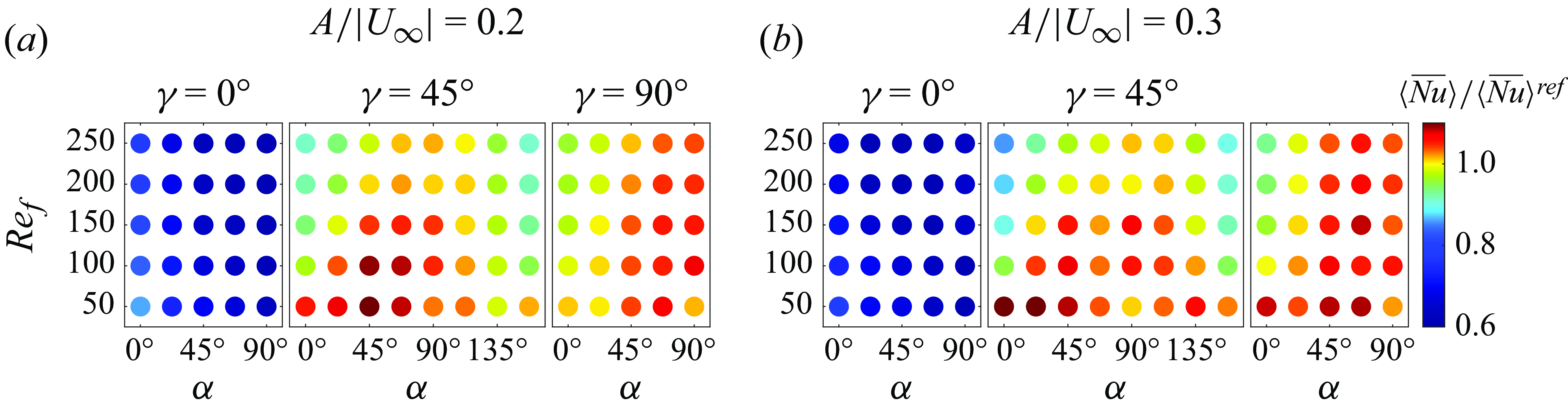
Figure 17. Ratio of $\langle \overline {Nu} \rangle$
for the oscillating plate to that of the stationary plate at the same total input power. Panels (a) and (b) correspond to
$\langle \overline {Nu} \rangle$
for the oscillating plate to that of the stationary plate at the same total input power. Panels (a) and (b) correspond to $A/|\boldsymbol{U}_{\infty }|=0.2$
and 0.3, respectively. The colours of the filled circles in the
$A/|\boldsymbol{U}_{\infty }|=0.2$
and 0.3, respectively. The colours of the filled circles in the $\alpha$
-
$\alpha$
- $Re_f$
plane correspond to different values of the ratio
$Re_f$
plane correspond to different values of the ratio $\langle \overline {Nu} \rangle / \langle \overline {Nu} \rangle ^{{ref}}$
, with
$\langle \overline {Nu} \rangle / \langle \overline {Nu} \rangle ^{{ref}}$
, with $\langle \overline {Nu} \rangle$
and
$\langle \overline {Nu} \rangle$
and $\langle \overline {Nu} \rangle ^{{ref}}$
computed for the oscillating and stationary plates at the same total input power evaluated with equation (5.5).
$\langle \overline {Nu} \rangle ^{{ref}}$
computed for the oscillating and stationary plates at the same total input power evaluated with equation (5.5).
Figure 17 shows the values of $\langle \overline {Nu} \rangle / \langle \overline {Nu} \rangle ^{{ref}}$
with coloured circles in the
$\langle \overline {Nu} \rangle / \langle \overline {Nu} \rangle ^{{ref}}$
with coloured circles in the $\alpha$
-
$\alpha$
- $Re_f$
plane for each
$Re_f$
plane for each $\gamma$
at
$\gamma$
at $A/|\boldsymbol{U}_{\infty }|=0.2$
(panel (a)) and 0.3 (panel (b)). Circles coloured orange to red show
$A/|\boldsymbol{U}_{\infty }|=0.2$
(panel (a)) and 0.3 (panel (b)). Circles coloured orange to red show $\langle \overline {Nu} \rangle / \langle \overline {Nu} \rangle ^{{ref}}\gt 1$
, i.e. when the oscillating plate outperforms the stationary plate. Such cases occur when
$\langle \overline {Nu} \rangle / \langle \overline {Nu} \rangle ^{{ref}}\gt 1$
, i.e. when the oscillating plate outperforms the stationary plate. Such cases occur when $\gamma =45^\circ$
and
$\gamma =45^\circ$
and $90^\circ$
but not when
$90^\circ$
but not when $\gamma =0^\circ$
, consistent with what we observe in figure 16(b). For
$\gamma =0^\circ$
, consistent with what we observe in figure 16(b). For $\gamma =45^\circ$
and
$\gamma =45^\circ$
and $90^\circ$
,
$90^\circ$
, $\langle \overline {Nu} \rangle / \langle \overline {Nu} \rangle ^{{ref}}$
is generally larger with more transverse oscillation (
$\langle \overline {Nu} \rangle / \langle \overline {Nu} \rangle ^{{ref}}$
is generally larger with more transverse oscillation ( $\alpha$
closer to
$\alpha$
closer to $90^\circ$
) and smaller
$90^\circ$
) and smaller $Re_f$
, but there are exceptions.
$Re_f$
, but there are exceptions.
We present Pareto fronts and performance measures for the fixed-flux case in Appendix F. The optimal cases are generally similar to those with fixed plate temperature.
6. Conclusion
We studied the effect of vortex dynamics on heat transfer for an oscillating plate in an oncoming flow with Reynolds number $Re_U = 100$
. We varied the oncoming flow direction (
$Re_U = 100$
. We varied the oncoming flow direction ( $\gamma$
) from in plane to transverse, the plate oscillation direction (
$\gamma$
) from in plane to transverse, the plate oscillation direction ( $\alpha$
) from in plane to transverse and studied the effects of the plate oscillation velocity, frequency and amplitude. Although our work is an extension of the work of Rahman & Tafti (Reference Rahman and Tafti2020a
) with an expanded parameter space, we investigated a variety of flow patterns and focused on how these flows influence local and global heat transfer, while Rahman & Tafti (Reference Rahman and Tafti2020a
) mainly studied the effect of the plunge velocity (similar to the oscillation velocity (
$\alpha$
) from in plane to transverse and studied the effects of the plate oscillation velocity, frequency and amplitude. Although our work is an extension of the work of Rahman & Tafti (Reference Rahman and Tafti2020a
) with an expanded parameter space, we investigated a variety of flow patterns and focused on how these flows influence local and global heat transfer, while Rahman & Tafti (Reference Rahman and Tafti2020a
) mainly studied the effect of the plunge velocity (similar to the oscillation velocity ( $A/|\boldsymbol{U}_{\infty }|$
) in our work) on the global Nusselt number without discussing the flow details.
$A/|\boldsymbol{U}_{\infty }|$
) in our work) on the global Nusselt number without discussing the flow details.
We classified the resulting vortex dynamics and heat transfer patterns into a small number of main categories. Steady plates provided benchmark flows, either steady Prandtl-boundary-layer-type flows (at $\gamma = 0^\circ$
) or von Kármán vortex wakes (at
$\gamma = 0^\circ$
) or von Kármán vortex wakes (at $\gamma = 45^\circ$
and
$\gamma = 45^\circ$
and $90^\circ$
). Without a natural wake frequency, many in-plane oncoming flows (
$90^\circ$
). Without a natural wake frequency, many in-plane oncoming flows ( $\gamma = 0^\circ$
) resulted in a periodic dynamics with the period of the plate oscillation. A few cases with transverse oscillation had period 1/2, up–down symmetry, and smaller heat transfer, and a few other cases at larger oscillation velocity (
$\gamma = 0^\circ$
) resulted in a periodic dynamics with the period of the plate oscillation. A few cases with transverse oscillation had period 1/2, up–down symmetry, and smaller heat transfer, and a few other cases at larger oscillation velocity ( $A/|\boldsymbol{U}_{\infty }|=0.3$
) were non-periodic and had larger heat transfer. With natural wake frequencies in addition to the plate frequency, oblique and transverse flows (
$A/|\boldsymbol{U}_{\infty }|=0.3$
) were non-periodic and had larger heat transfer. With natural wake frequencies in addition to the plate frequency, oblique and transverse flows ( $\gamma = 45^\circ$
and
$\gamma = 45^\circ$
and $90^\circ$
) resulted in a dynamics that was almost periodic at multiples of the plate oscillation period, or non-periodic, the latter occurring mainly with more transverse oscillations at larger velocity (
$90^\circ$
) resulted in a dynamics that was almost periodic at multiples of the plate oscillation period, or non-periodic, the latter occurring mainly with more transverse oscillations at larger velocity ( $A/|\boldsymbol{U}_{\infty }|=0.3$
). Note that the classification is based on the regularity of the vortex dynamics instead of heat transfer performance, although non-periodic cases are often associated with stronger vortices and thus better heat transfer.
$A/|\boldsymbol{U}_{\infty }|=0.3$
). Note that the classification is based on the regularity of the vortex dynamics instead of heat transfer performance, although non-periodic cases are often associated with stronger vortices and thus better heat transfer.
The steady plate has different vorticity patterns at different plate orientations ( $\gamma$
). Including the plate oscillation adds many new features to the vorticity patterns and alters the local heat transfer distributions dramatically. With in-plane flow (
$\gamma$
). Including the plate oscillation adds many new features to the vorticity patterns and alters the local heat transfer distributions dramatically. With in-plane flow ( $\gamma =0^\circ$
) and no plate oscillation, heat transfer is maximum at the leading edge and temperature is maximum near the trailing edge. Adding in-plane oscillation (
$\gamma =0^\circ$
) and no plate oscillation, heat transfer is maximum at the leading edge and temperature is maximum near the trailing edge. Adding in-plane oscillation ( $\alpha =0^\circ$
) gives modest improvements near the trailing edge, but the boundary layers remain intact. With oblique (
$\alpha =0^\circ$
) gives modest improvements near the trailing edge, but the boundary layers remain intact. With oblique ( $\alpha =45^\circ$
) and transverse (
$\alpha =45^\circ$
) and transverse ( $\alpha =90^\circ$
) oscillations, vortices are shed from the edges, decreasing heat transfer near the leading edge and but enhancing it over the rest of the plate, giving a net improvement. With oblique and transverse flow (
$\alpha =90^\circ$
) oscillations, vortices are shed from the edges, decreasing heat transfer near the leading edge and but enhancing it over the rest of the plate, giving a net improvement. With oblique and transverse flow ( $\gamma = 45^\circ$
and
$\gamma = 45^\circ$
and $90^\circ$
), the heat transfer is controlled by the formation of large regions of vorticity, from the merging of vortices shed over multiple cycles. These ‘vortex groups’ tend to form near one edge and enhance heat transfer mainly at the opposite edge. After many cycles the group detaches from one edge, a new group of oppositely signed vorticity forms near the other edge, and the cycle repeats. The net effect of the vortex groups is to greatly increase heat transfer on the wake side, to a level comparable to that on the side facing the oncoming flow. On the wake side, heat transfer is increased most on the portion farther from the vortex group, which draws colder fluid there. Although the local heat transfer patterns for different
$90^\circ$
), the heat transfer is controlled by the formation of large regions of vorticity, from the merging of vortices shed over multiple cycles. These ‘vortex groups’ tend to form near one edge and enhance heat transfer mainly at the opposite edge. After many cycles the group detaches from one edge, a new group of oppositely signed vorticity forms near the other edge, and the cycle repeats. The net effect of the vortex groups is to greatly increase heat transfer on the wake side, to a level comparable to that on the side facing the oncoming flow. On the wake side, heat transfer is increased most on the portion farther from the vortex group, which draws colder fluid there. Although the local heat transfer patterns for different $\gamma$
are quite different, when we take an average over the plate to compute the global heat transfer, the differences are significantly reduced.
$\gamma$
are quite different, when we take an average over the plate to compute the global heat transfer, the differences are significantly reduced.
The global heat transfer (figure 7) was most strongly affected by the oscillation velocity ( $A/|\boldsymbol{U}_{\infty }|$
) and direction (
$A/|\boldsymbol{U}_{\infty }|$
) and direction ( $\alpha$
), being larger with a faster and more transverse oscillation. In this case the shed vortices were stronger and the dynamics was less periodic, enhancing mixing in the wake region. The effect of
$\alpha$
), being larger with a faster and more transverse oscillation. In this case the shed vortices were stronger and the dynamics was less periodic, enhancing mixing in the wake region. The effect of $\gamma$
was relatively small for the cases with better heat transfer (
$\gamma$
was relatively small for the cases with better heat transfer ( $\gamma \neq 0, \alpha \neq 0$
). For a given oscillation velocity (
$\gamma \neq 0, \alpha \neq 0$
). For a given oscillation velocity ( $A/|\boldsymbol{U}_{\infty }|$
), increasing the oscillation frequency (
$A/|\boldsymbol{U}_{\infty }|$
), increasing the oscillation frequency ( $Re_f$
) while decreasing the oscillation amplitude had relatively little effect on the global heat transfer, except in a few cases with transitions between patterns of vortex dynamics. Local heat transfer was altered by
$Re_f$
) while decreasing the oscillation amplitude had relatively little effect on the global heat transfer, except in a few cases with transitions between patterns of vortex dynamics. Local heat transfer was altered by $\gamma$
and
$\gamma$
and $Re_f$
, however, through changes in the sizes and locations of shed vortices.
$Re_f$
, however, through changes in the sizes and locations of shed vortices.
Another mechanism we found was that vortex grouping helped trap the vorticity and enhanced mixing near the plate. We already mentioned that the shed vorticity was stronger with more transverse oscillations ( $\alpha$
closer to
$\alpha$
closer to $90^\circ$
). At
$90^\circ$
). At $\gamma = 45^\circ$
, pairs of cases (supplementary angles) have the same degree of transverse motion but one (
$\gamma = 45^\circ$
, pairs of cases (supplementary angles) have the same degree of transverse motion but one ( $\alpha \lt 90^\circ$
) moves more along the oncoming flow and the other across it (
$\alpha \lt 90^\circ$
) moves more along the oncoming flow and the other across it ( $\alpha \gt 90^\circ$
). The former case leads to stronger, more compact vortex groups and somewhat better heat transfer. Vortex grouping was also seen in some cases of in-plane flow (
$\alpha \gt 90^\circ$
). The former case leads to stronger, more compact vortex groups and somewhat better heat transfer. Vortex grouping was also seen in some cases of in-plane flow ( $\gamma =0^\circ$
) with transverse oscillation, where it also enhanced heat transfer.
$\gamma =0^\circ$
) with transverse oscillation, where it also enhanced heat transfer.
We considered plates with fixed temperature or fixed heat flux. In general the same parameters are optimal in both cases, with some variability when the maximum (rather than average) plate temperature is considered in the latter case.
We also considered the input power needed to oscillate the plate and to drive the entire flow including the oncoming flow. The input power can be neglected if the oncoming flow is provided by ambient flows in the environment and the plate oscillation occurs through passive fluid–structure interaction. In this case the best case, the one that maximises $\langle \overline {Nu} \rangle$
, has
$\langle \overline {Nu} \rangle$
, has $A/|\boldsymbol{U}_{\infty }|=0.3$
,
$A/|\boldsymbol{U}_{\infty }|=0.3$
, $\alpha = 90^\circ$
and
$\alpha = 90^\circ$
and $\gamma = 45^\circ$
(with
$\gamma = 45^\circ$
(with $\gamma = 90^\circ$
very close). If power is needed to oscillate the plate, optimality is given by the Pareto front in
$\gamma = 90^\circ$
very close). If power is needed to oscillate the plate, optimality is given by the Pareto front in $\langle \overline {Nu} \rangle$
–
$\langle \overline {Nu} \rangle$
– $\langle \tilde {P}_{{body}} \rangle$
space. The front includes the steady plate with
$\langle \tilde {P}_{{body}} \rangle$
space. The front includes the steady plate with $\gamma = 0^\circ$
(with
$\gamma = 0^\circ$
(with $\langle \tilde {P}_{{body}} \rangle$
= 0) as well as many oscillating plates with larger
$\langle \tilde {P}_{{body}} \rangle$
= 0) as well as many oscillating plates with larger $\langle \overline {Nu} \rangle$
and non-zero
$\langle \overline {Nu} \rangle$
and non-zero $\langle \tilde {P}_{{body}} \rangle$
. These cases have
$\langle \tilde {P}_{{body}} \rangle$
. These cases have $A/|\boldsymbol{U}_{\infty }|=0.2$
and 0.3,
$A/|\boldsymbol{U}_{\infty }|=0.2$
and 0.3, $0^\circ \leqslant \alpha \leqslant 90^\circ$
and
$0^\circ \leqslant \alpha \leqslant 90^\circ$
and $\gamma = 45^\circ$
and
$\gamma = 45^\circ$
and $90^\circ$
. If power is also needed to drive the oncoming flow, the optimal case (the Pareto front in
$90^\circ$
. If power is also needed to drive the oncoming flow, the optimal case (the Pareto front in $\langle \overline {Nu} \rangle$
–
$\langle \overline {Nu} \rangle$
– $\langle \tilde {P}_{{total}} \rangle$
space) is the steady plate with
$\langle \tilde {P}_{{total}} \rangle$
space) is the steady plate with $\gamma = 0^\circ$
. If we restrict
$\gamma = 0^\circ$
. If we restrict $\gamma$
to
$\gamma$
to $45^\circ$
and
$45^\circ$
and $90^\circ$
, then many of the oscillating-plate cases that are Pareto optimal in
$90^\circ$
, then many of the oscillating-plate cases that are Pareto optimal in $\langle \overline {Nu} \rangle$
–
$\langle \overline {Nu} \rangle$
– $\langle \tilde {P}_{{body}} \rangle$
space are also Pareto optimal in
$\langle \tilde {P}_{{body}} \rangle$
space are also Pareto optimal in $\langle \overline {Nu} \rangle$
–
$\langle \overline {Nu} \rangle$
– $\langle \tilde {P}_{{total}} \rangle$
space.
$\langle \tilde {P}_{{total}} \rangle$
space.
We used a Prandtl number of 0.7, corresponding to air at standard temperature and pressure. Changing $Pr$
will not affect our flows as the flow is independent of the temperature field in our problem. However, the temperature fields and resulting Nusselt numbers will be affected. In general, increasing
$Pr$
will not affect our flows as the flow is independent of the temperature field in our problem. However, the temperature fields and resulting Nusselt numbers will be affected. In general, increasing $Pr$
decreases the thermal boundary layer thickness, which increases the Nusselt number. At
$Pr$
decreases the thermal boundary layer thickness, which increases the Nusselt number. At $Pr = 0.7$
, the thermal and velocity boundary layers are comparable in thickness. If
$Pr = 0.7$
, the thermal and velocity boundary layers are comparable in thickness. If $Pr \ll 1$
(
$Pr \ll 1$
( $\gg 1$
), the thermal boundary layer is much thicker (thinner) than the velocity boundary layer, and the Nusselt number increases as different power laws of
$\gg 1$
), the thermal boundary layer is much thicker (thinner) than the velocity boundary layer, and the Nusselt number increases as different power laws of $Pr$
in these two regimes for steady boundary layer flow (Schlichting & Gersten Reference Schlichting and Gersten2017). There are some studies on the effect of
$Pr$
in these two regimes for steady boundary layer flow (Schlichting & Gersten Reference Schlichting and Gersten2017). There are some studies on the effect of $Pr$
on oscillatory flows past fixed bodies at
$Pr$
on oscillatory flows past fixed bodies at $Re$
similar to our study (Dhiman et al. Reference Dhiman, Chhabra, Sharma and Eswaran2006; Chandra & Chhabra Reference Chandra and Chhabra2011; Sarkar, Dalal & Biswas Reference Sarkar, Dalal and Biswas2011; Chatterjee & Mondal Reference Chatterjee and Mondal2012; Ali et al. Reference Ali, Arif, Haider and Shamim2024), but fewer studies consider oscillating bodies, although the work of Cheng, Hong & Aung (Reference Cheng, Hong and Aung1997) is one example. In general, these studies find, as for steady flows, that increasing
$Re$
similar to our study (Dhiman et al. Reference Dhiman, Chhabra, Sharma and Eswaran2006; Chandra & Chhabra Reference Chandra and Chhabra2011; Sarkar, Dalal & Biswas Reference Sarkar, Dalal and Biswas2011; Chatterjee & Mondal Reference Chatterjee and Mondal2012; Ali et al. Reference Ali, Arif, Haider and Shamim2024), but fewer studies consider oscillating bodies, although the work of Cheng, Hong & Aung (Reference Cheng, Hong and Aung1997) is one example. In general, these studies find, as for steady flows, that increasing $Pr$
increases the Nusselt number by thinning the thermal boundary layer. When
$Pr$
increases the Nusselt number by thinning the thermal boundary layer. When $Pr \ll 1$
, the thermal boundary is thicker than the flow boundary layer, and may be comparable in size to, or larger than, the shed vortices. This can make the temperature field less sensitive to the vortex dynamics. In contrast, when
$Pr \ll 1$
, the thermal boundary is thicker than the flow boundary layer, and may be comparable in size to, or larger than, the shed vortices. This can make the temperature field less sensitive to the vortex dynamics. In contrast, when $Pr \gg 1$
, the thermal boundary is thinner than the flow boundary layer. However, the pattern of temperature contours is still strongly determined by the vorticity pattern, since the flow determines the temperature field. Thus the temperature boundary layer separates and rolls up on length scales set by the vortices. As
$Pr \gg 1$
, the thermal boundary is thinner than the flow boundary layer. However, the pattern of temperature contours is still strongly determined by the vorticity pattern, since the flow determines the temperature field. Thus the temperature boundary layer separates and rolls up on length scales set by the vortices. As $Pr$
varies in our problem, we expect broadly similar trends to those mentioned above. However, it is difficult to give more detailed predictions without simulating the system at various
$Pr$
varies in our problem, we expect broadly similar trends to those mentioned above. However, it is difficult to give more detailed predictions without simulating the system at various $Pr$
, which is beyond the scope of this study.
$Pr$
, which is beyond the scope of this study.
Supplementary movies
Supplementary movies are available at https://doi.org/10.1017/jfm.2025.10201.
Funding
This research was supported by the NSF-DMS Applied Mathematics program under award number DMS-2204900.
Declaration of interests
The authors report no conflict of interest.
Appendix A. Grid details
In this appendix, we provide details about the grid generation and mesh point distributions. The method used here to generate a non-uniform mesh (as shown in figure 2) is modified from that used by Alben (Reference Alben2021a ).
To generate grid points in the $x$
direction, we first specify
$x$
direction, we first specify $m_2$
,
$m_2$
, $m_1$
and
$m_1$
and $m_3$
, the numbers of grid points on the plate (
$m_3$
, the numbers of grid points on the plate ( $0\leqslant x\leqslant 1$
), on the interval from the left edge of the plate to the left boundary of the computational domain (
$0\leqslant x\leqslant 1$
), on the interval from the left edge of the plate to the left boundary of the computational domain ( $-L_{x1}\leqslant x \leqslant 0$
), and on the interval from the right edge of the plate to the right boundary of the computational domain (
$-L_{x1}\leqslant x \leqslant 0$
), and on the interval from the right edge of the plate to the right boundary of the computational domain ( $1\leqslant x \leqslant L_{x2}$
), respectively. Then we generate uniform grids (
$1\leqslant x \leqslant L_{x2}$
), respectively. Then we generate uniform grids ( $X$
) for each segment and stretch them as follows:
$X$
) for each segment and stretch them as follows:
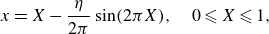 \begin{align}&\qquad\qquad\qquad x = X-\frac {\eta }{2\pi }\sin (2\pi X), \quad 0\leqslant X \leqslant 1, \end{align}
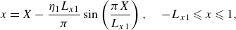 \begin{align}&\qquad\qquad x = X-\frac {\eta _1 L_{x1}}{\pi }\sin \left (\displaystyle \frac {\pi X}{L_{x1}}\right ), \quad -L_{x1}\leqslant x \leqslant 1, \end{align}
 \begin{align}& x = 1+X-\frac {\eta _2 (L_{x2}-1)}{\pi }\sin \left (\displaystyle \frac {\pi X}{L_{x2}-1}\right ), \quad 0\leqslant X\leqslant L_{x2}-1. \end{align}
Here, $\eta$
,
$\eta$
, $\eta _1$
and
$\eta _1$
and $\eta _2$
are the three factors controlling grid spacing. On the plate (A1a
), the uniform grid spacing
$\eta _2$
are the three factors controlling grid spacing. On the plate (A1a
), the uniform grid spacing $\Delta X$
is compressed by approximately
$\Delta X$
is compressed by approximately $1-\eta$
near the edges and stretched by approximately
$1-\eta$
near the edges and stretched by approximately $1+\eta$
in the centre. Similarly, by equations (A1b
) and (A1c
), the grid points cluster near the plate edges and gradually spread out toward the boundary of the computational domain. In our simulation, we set
$1+\eta$
in the centre. Similarly, by equations (A1b
) and (A1c
), the grid points cluster near the plate edges and gradually spread out toward the boundary of the computational domain. In our simulation, we set $\eta =0.95$
. This number is also suggested by Alben (Reference Alben2021a
), which is close enough to 1 to reduce the errors at the plate edges. In order to keep the grid size similar at the two sides of the plate edge, we set
$\eta =0.95$
. This number is also suggested by Alben (Reference Alben2021a
), which is close enough to 1 to reduce the errors at the plate edges. In order to keep the grid size similar at the two sides of the plate edge, we set $\eta _1$
and
$\eta _1$
and $\eta _2$
by imposing
$\eta _2$
by imposing
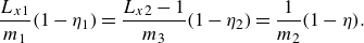 \begin{equation} \frac {L_{x1}}{m_1}(1-\eta _1) = \frac {L_{x2}-1}{m_3}(1-\eta _2) = \frac {1}{m_2}(1-\eta ). \end{equation}
In a similar way, we first create a uniform grid $Y$
by assigning
$Y$
by assigning $n_1$
and
$n_1$
and $n_2$
points below and above the plate, respectively. Then the grid is deformed using
$n_2$
points below and above the plate, respectively. Then the grid is deformed using
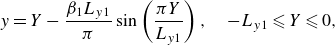 \begin{align}& y = Y-\frac {\beta _1 L_{y1}}{\pi }\sin \left (\frac {\pi Y}{L_{y1}} \right ), \quad -L_{y1}\leqslant Y \leqslant 0, \end{align}
 \begin{align}&\,\, y = Y-\frac {\beta _2 L_{y2}}{\pi }\sin \left (\frac {\pi Y}{L_{y2}} \right ), \quad 0\leqslant Y \leqslant L_{y2}. \end{align}
The grid size along $y$
is smallest near the plate and gradually increases toward the bottom and top boundaries of the computational domain. In our simulation, we use
$y$
is smallest near the plate and gradually increases toward the bottom and top boundaries of the computational domain. In our simulation, we use $\beta _1=0.95$
. Again, to ensure the grid sizes at the top and bottom of the plate are similar,
$\beta _1=0.95$
. Again, to ensure the grid sizes at the top and bottom of the plate are similar, $\beta _2$
is computed by imposing
$\beta _2$
is computed by imposing
 \begin{equation} \frac {L_{y1}}{n_1}(1-\beta _1) = \frac {L_{y2}}{n_2}(1-\beta _2). \end{equation}
In table 2, we report the number of grid cells for each segment in (A1) and (A3) as well as the smallest and the largest grid spacings in the $x$
and
$x$
and $y$
directions, respectively. The mesh near the plate is dense to capture the sharp gradients in flow velocity and temperature there. For
$y$
directions, respectively. The mesh near the plate is dense to capture the sharp gradients in flow velocity and temperature there. For $\gamma =0^\circ$
, we have approximately 40 cells in the
$\gamma =0^\circ$
, we have approximately 40 cells in the $y$
direction across the boundary layer thickness (calculated using the Blasius approximation) at the plate centre (
$y$
direction across the boundary layer thickness (calculated using the Blasius approximation) at the plate centre ( $x=0.5$
). The larger grid cells are close to the boundaries of the computational domain. For
$x=0.5$
). The larger grid cells are close to the boundaries of the computational domain. For $\gamma =0^\circ$
and
$\gamma =0^\circ$
and $\gamma =45^\circ$
, the mesh near the left boundary is more sparse than that near the right boundary because the left boundary is the inlet and the flow is almost uniform.
$\gamma =45^\circ$
, the mesh near the left boundary is more sparse than that near the right boundary because the left boundary is the inlet and the flow is almost uniform.
Table 2. The numbers of grid cells in different regions and the minimal and maximal grid sizes in the $x$
and
$x$
and $y$
directions.
$y$
directions.
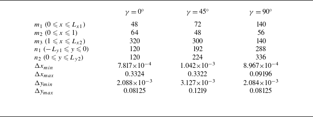
Appendix B. Grid independence study
In this appendix, we give numerical tests to explain the chosen domain and grid sizes in table 1. We vary the domain size according to the plate orientation $\gamma$
to avoid boundary effects. For different
$\gamma$
to avoid boundary effects. For different $\gamma$
, we compare the time series of the global heat transfer quantities,
$\gamma$
, we compare the time series of the global heat transfer quantities, $\overline {Nu}$
,
$\overline {Nu}$
, $T_{max }$
and
$T_{max }$
and $T_{{avg}}$
using different grid sizes with different domain sizes. We also investigate the variation of the time averages of the global heat transfer quantities when we average over different numbers of oscillation cycles.
$T_{{avg}}$
using different grid sizes with different domain sizes. We also investigate the variation of the time averages of the global heat transfer quantities when we average over different numbers of oscillation cycles.
When the oncoming flow is horizontal ( $\gamma = 0^\circ$
), we use a computational domain with horizontal length approximately twice the vertical length. In figure 18, we compare the time series of the three global heat transfer quantities in three computational domains. The number of grid points is roughly proportional to the domain size. For example, the ratios of
$\gamma = 0^\circ$
), we use a computational domain with horizontal length approximately twice the vertical length. In figure 18, we compare the time series of the three global heat transfer quantities in three computational domains. The number of grid points is roughly proportional to the domain size. For example, the ratios of $x$
grid points satisfy:
$x$
grid points satisfy: $288/224\approx (8+10)/(6+8)$
and
$288/224\approx (8+10)/(6+8)$
and $352/288\approx (10+12)/(8+10)$
. We find that domain 2 with the intermediate mesh of
$352/288\approx (10+12)/(8+10)$
. We find that domain 2 with the intermediate mesh of $432\times 240$
can produce results with sufficient accuracy. Since it is a periodic flow, the time averages are taken over the last 2 cycles of the plate oscillation. This mesh is also studied in a case with a non-periodic, irregular dynamics in figure 19. Here, close agreement with different meshes and domain sizes is only observed in the first several cycles. In panel (c), we show the time-averaged quantities
$432\times 240$
can produce results with sufficient accuracy. Since it is a periodic flow, the time averages are taken over the last 2 cycles of the plate oscillation. This mesh is also studied in a case with a non-periodic, irregular dynamics in figure 19. Here, close agreement with different meshes and domain sizes is only observed in the first several cycles. In panel (c), we show the time-averaged quantities $\langle \overline {Nu} \rangle$
,
$\langle \overline {Nu} \rangle$
, $\max {T_{max }}$
and
$\max {T_{max }}$
and $\langle T_{max } \rangle$
using averages over different numbers of cycles. Note that the number of cycles is counted backwards starting from the final time. For example, if the number of cycles is 2, it means that the last 2 cycles are used to compute the time averages. The averages show stronger variations when close to the maximum number of cycles is used, since then the cycles from the initial transient are included. As shown in panels (c) and (d),
$\langle T_{max } \rangle$
using averages over different numbers of cycles. Note that the number of cycles is counted backwards starting from the final time. For example, if the number of cycles is 2, it means that the last 2 cycles are used to compute the time averages. The averages show stronger variations when close to the maximum number of cycles is used, since then the cycles from the initial transient are included. As shown in panels (c) and (d), $\langle \overline {Nu} \rangle$
starts to increase and
$\langle \overline {Nu} \rangle$
starts to increase and $T_{{avg}}$
starts to decrease if more than 54 cycles are used. This is because
$T_{{avg}}$
starts to decrease if more than 54 cycles are used. This is because $\overline {Nu}$
rapidly decreases from a very high value while
$\overline {Nu}$
rapidly decreases from a very high value while $T_{{avg}}$
increases from 0 (recalling that
$T_{{avg}}$
increases from 0 (recalling that $T(t=0) =0$
in the fixed-heat-flux case) over the first several cycles, as shown in panels (a) and (b). Therefore, time averages should be taken over approximately 5–10 cycles fewer than the maximum (
$T(t=0) =0$
in the fixed-heat-flux case) over the first several cycles, as shown in panels (a) and (b). Therefore, time averages should be taken over approximately 5–10 cycles fewer than the maximum ( $t_{{end}}$
), e.g. 50–55 cycles in figure 19, where the time averages are nearly flat. It is somewhat coincidental that the time-averaged results with the coarsest and finest meshes are closer, because the agreements between the time series in panels (a) and (b) are less close: in panel (a), the finest mesh agrees better with the middle mesh than the coarsest mesh. In this case, we take the last
$t_{{end}}$
), e.g. 50–55 cycles in figure 19, where the time averages are nearly flat. It is somewhat coincidental that the time-averaged results with the coarsest and finest meshes are closer, because the agreements between the time series in panels (a) and (b) are less close: in panel (a), the finest mesh agrees better with the middle mesh than the coarsest mesh. In this case, we take the last $40$
cycles to compute the time-averaged quantities. For the other non-periodic and irregular cases, we do similar comparisons, and the time span chosen to compute the time average is usually at least half of the total simulated time.
$40$
cycles to compute the time-averaged quantities. For the other non-periodic and irregular cases, we do similar comparisons, and the time span chosen to compute the time average is usually at least half of the total simulated time.
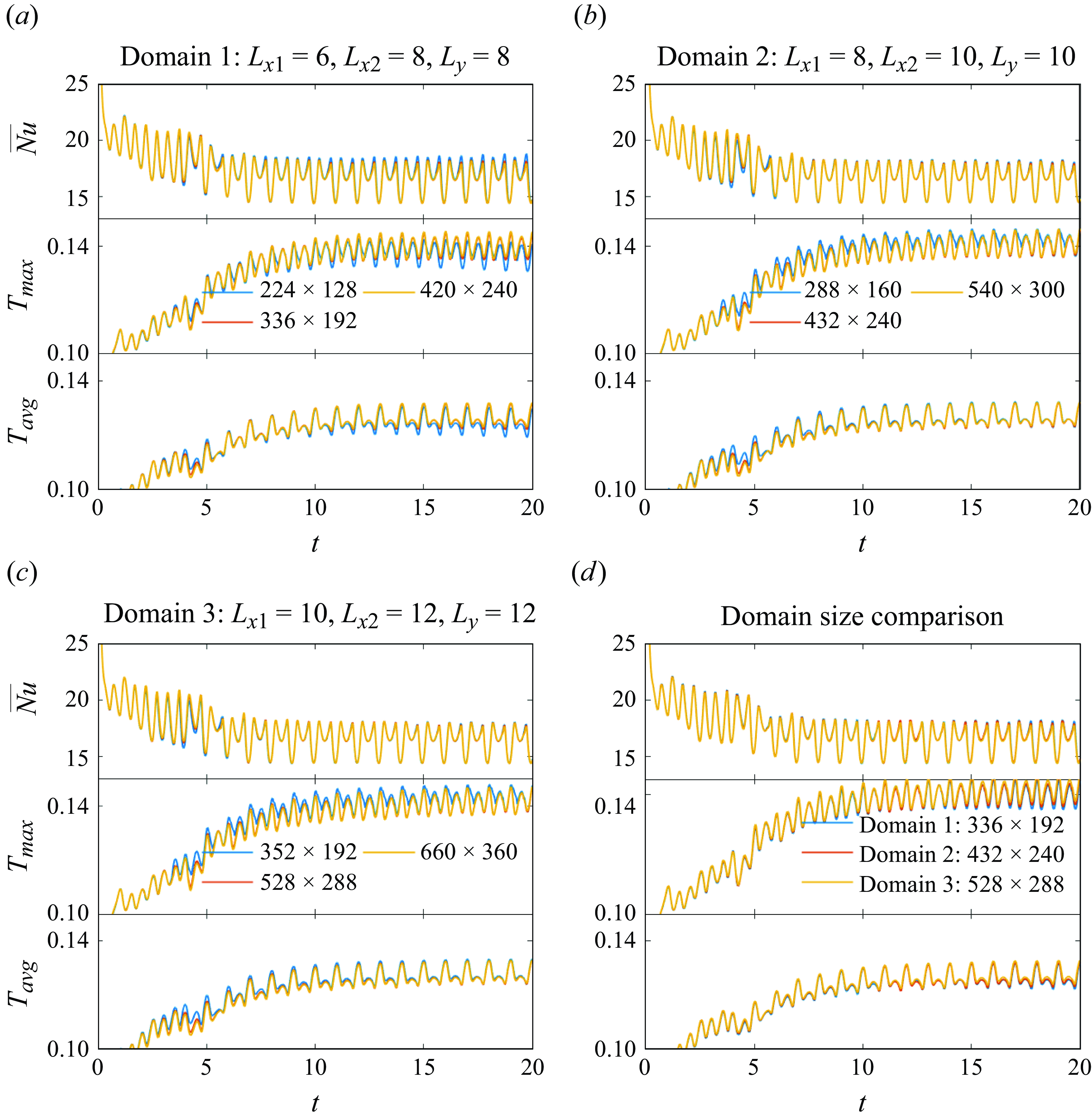
Figure 18. Comparisons of the time series of the global heat transfer quantities $\overline {Nu}$
,
$\overline {Nu}$
, $T_{max }$
and
$T_{max }$
and $T_{{avg}}$
with different domain sizes and grid sizes when the oncoming flow is horizontal (
$T_{{avg}}$
with different domain sizes and grid sizes when the oncoming flow is horizontal ( $\gamma = 0^\circ$
). The other simulation parameters are:
$\gamma = 0^\circ$
). The other simulation parameters are: $Re_f=100$
,
$Re_f=100$
, $Re_U=100$
,
$Re_U=100$
, $\alpha = 90^\circ$
and
$\alpha = 90^\circ$
and $A/|\boldsymbol{U}_{\infty }|=0.2$
.
$A/|\boldsymbol{U}_{\infty }|=0.2$
.
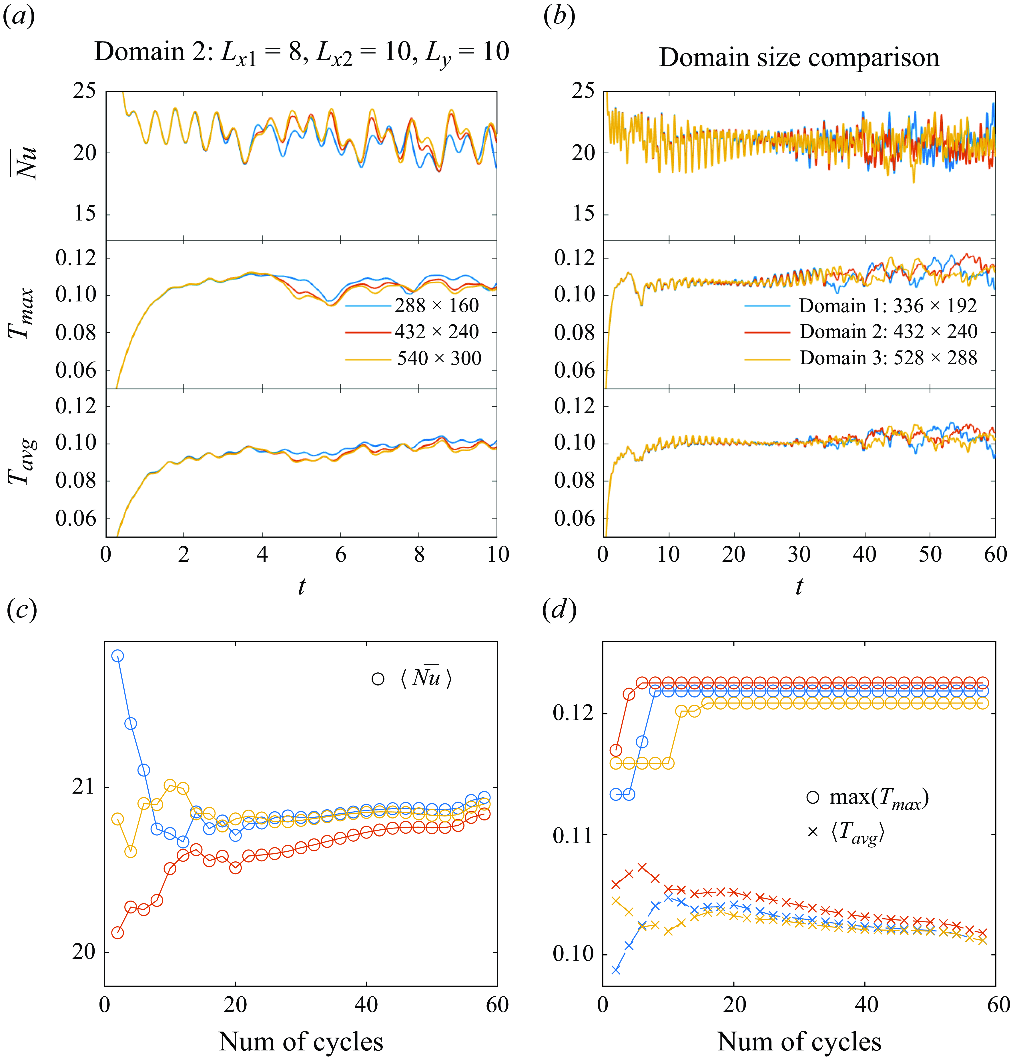
Figure 19. Comparisons of the global heat transfer quantities $\overline {Nu}$
,
$\overline {Nu}$
, $T_{max }$
and
$T_{max }$
and $T_{{avg}}$
, and their time averages, using different grid sizes (a) and domain sizes (b) when the oncoming flow is horizontal (
$T_{{avg}}$
, and their time averages, using different grid sizes (a) and domain sizes (b) when the oncoming flow is horizontal ( $\gamma = 0^\circ$
) and
$\gamma = 0^\circ$
) and $Re_f=200$
,
$Re_f=200$
, $Re_U=100$
,
$Re_U=100$
, $\alpha = 90^\circ$
and
$\alpha = 90^\circ$
and $A/|\boldsymbol{U}_{\infty }|=0.3$
. (c) Time-averaged global heat transfer quantities using different numbers of cycles in the three computational domains. The correspondence between the curve colour and the domain size is the same as in panel (b).
$A/|\boldsymbol{U}_{\infty }|=0.3$
. (c) Time-averaged global heat transfer quantities using different numbers of cycles in the three computational domains. The correspondence between the curve colour and the domain size is the same as in panel (b).
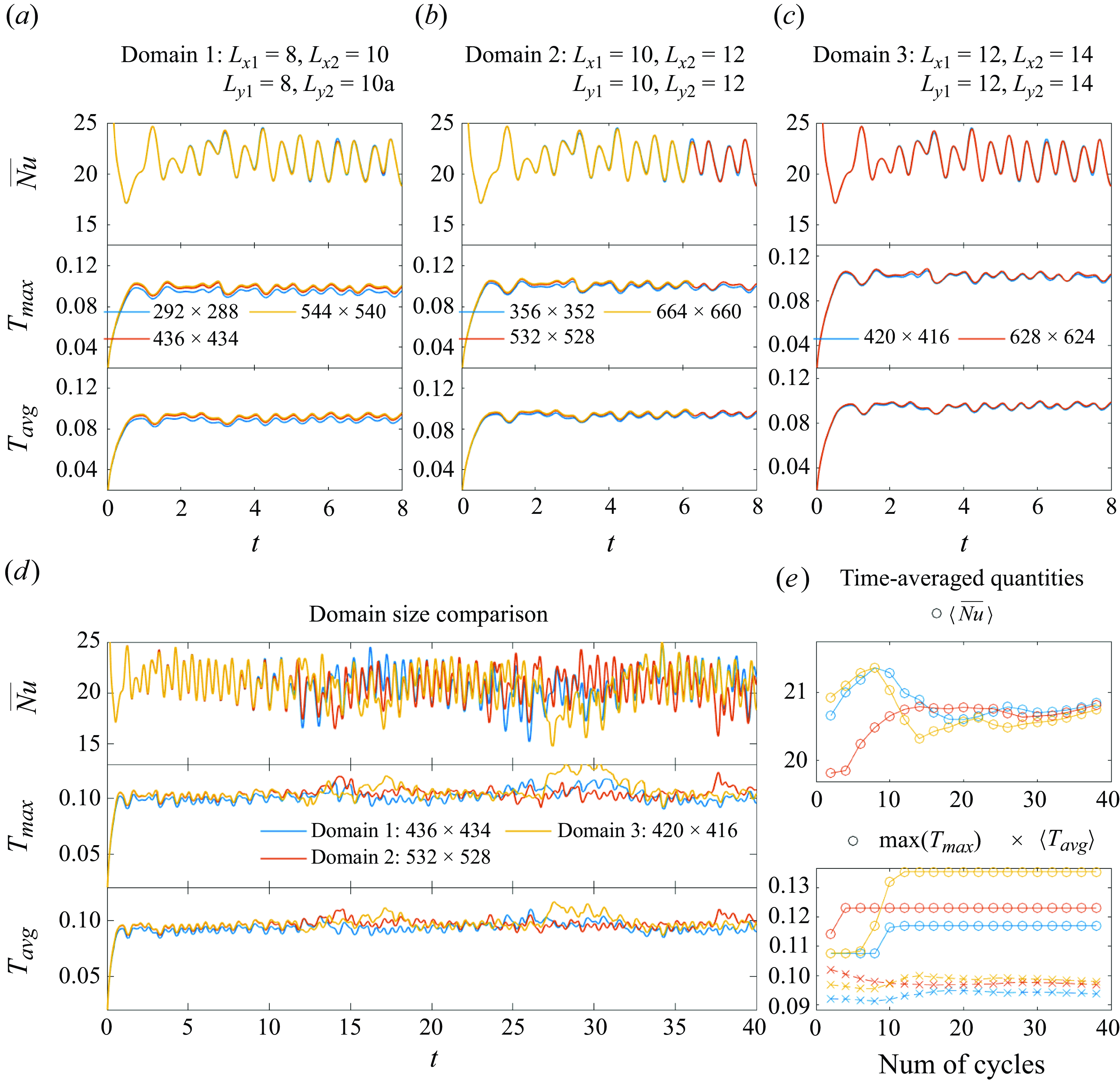
Figure 20. Comparisons of the global heat transfer quantities $\overline {Nu}$
,
$\overline {Nu}$
, $T_{max }$
and
$T_{max }$
and $T_{{avg}}$
, and their time averages, using different domain and grid sizes when the oncoming flow is oblique (
$T_{{avg}}$
, and their time averages, using different domain and grid sizes when the oncoming flow is oblique ( $\gamma = 45^\circ$
) and
$\gamma = 45^\circ$
) and $Re_f=100$
,
$Re_f=100$
, $Re_U=100$
,
$Re_U=100$
, $\alpha = 90^\circ$
and
$\alpha = 90^\circ$
and $A/|\boldsymbol{U}_{\infty }|=0.3$
. The correspondence between the curve colour and the domain size in panel (e) is the same as in panel (d).
$A/|\boldsymbol{U}_{\infty }|=0.3$
. The correspondence between the curve colour and the domain size in panel (e) is the same as in panel (d).

Figure 21. Comparisons of the global heat transfer quantities $\overline {Nu}$
,
$\overline {Nu}$
, $T_{max }$
and
$T_{max }$
and $T_{{avg}}$
, and their time averages, using different domain and grid sizes when the oncoming flow is transverse (
$T_{{avg}}$
, and their time averages, using different domain and grid sizes when the oncoming flow is transverse ( $\gamma = 90^\circ$
) and
$\gamma = 90^\circ$
) and $Re_f=100$
,
$Re_f=100$
, $Re_U=100$
,
$Re_U=100$
, $A=0.3$
,
$A=0.3$
, $\alpha = 60^\circ$
and
$\alpha = 60^\circ$
and $A/|\boldsymbol{U}_{\infty }|=0.3$
. The correspondence between the curve colour and the domain size in panel (e) is the same as in panel (d).
$A/|\boldsymbol{U}_{\infty }|=0.3$
. The correspondence between the curve colour and the domain size in panel (e) is the same as in panel (d).
For the oblique oncoming flow ( $\gamma =45^\circ$
), we use a square computational domain since the oncoming flow has equal horizontal and vertical components. Panels (a), (b) and (c) of figure 20 show the time series of the three global heat transfer quantities computed with different domain sizes. In each computation domain, we have good agreement between the results at different grid sizes. Compared with the fixed-temperature results, we find that the fixed-heat-flux results are more sensitive to the grid and domain sizes: in panels (a) and (b),
$\gamma =45^\circ$
), we use a square computational domain since the oncoming flow has equal horizontal and vertical components. Panels (a), (b) and (c) of figure 20 show the time series of the three global heat transfer quantities computed with different domain sizes. In each computation domain, we have good agreement between the results at different grid sizes. Compared with the fixed-temperature results, we find that the fixed-heat-flux results are more sensitive to the grid and domain sizes: in panels (a) and (b), $T_{max }$
and
$T_{max }$
and $T_{{avg}}$
on the coarsest mesh are noticeably smaller, unlike
$T_{{avg}}$
on the coarsest mesh are noticeably smaller, unlike $\overline {Nu}$
. We compare the results with different computational domain sizes in panel (d). The middle mesh is chosen for domains 1 and 2 whereas the coarsest mesh is chosen for domain 3 because its results agree well with those of the finest mesh. In the first several cycles of plate oscillations,
$\overline {Nu}$
. We compare the results with different computational domain sizes in panel (d). The middle mesh is chosen for domains 1 and 2 whereas the coarsest mesh is chosen for domain 3 because its results agree well with those of the finest mesh. In the first several cycles of plate oscillations, $T_{max }$
and
$T_{max }$
and $T_{{avg}}$
for domains 2 and 3 agree well and are smaller for domain 1. Since boundary effects are more apparent for domain 1 we use domain 3 with the
$T_{{avg}}$
for domains 2 and 3 agree well and are smaller for domain 1. Since boundary effects are more apparent for domain 1 we use domain 3 with the $420\times 416$
grid because it is moderately expensive computationally. This case is non-periodic and irregular, as shown by the time series after 15 cycles. However, the time-averaged
$420\times 416$
grid because it is moderately expensive computationally. This case is non-periodic and irregular, as shown by the time series after 15 cycles. However, the time-averaged $\langle \overline {Nu} \rangle$
and
$\langle \overline {Nu} \rangle$
and $\langle T_{{avg}} \rangle$
in the three domains using more than 15 cycles of oscillations agree well, as shown in panel (e). The large variations in
$\langle T_{{avg}} \rangle$
in the three domains using more than 15 cycles of oscillations agree well, as shown in panel (e). The large variations in $\max (T_{max })$
are expected because, as the temperature of the hottest spot of the plate at one moment, it is sensitive to the irregular dynamics.
$\max (T_{max })$
are expected because, as the temperature of the hottest spot of the plate at one moment, it is sensitive to the irregular dynamics.
Finally, we show the convergence study for transverse oncoming flow ( $\gamma =90^\circ$
) in figure 21. Similar to the case of
$\gamma =90^\circ$
) in figure 21. Similar to the case of $\gamma =0^\circ$
, the computational domain for
$\gamma =0^\circ$
, the computational domain for $\gamma =90^\circ$
has a vertical dimension approximately twice the horizontal dimension. The case shown is not periodic but not as irregular as the case in figure 20, as the time series computed in different domains and with different grid sizes tend to agree for the entire simulated time. We again observe that the results with fixed heat flux are more sensitive to the domain size and grid size. For this case domain 1 is less accurate for the global heat transfer quantities, as shown in panels (d) and (e). Based on the comparisons in panels (a)–(e), we choose domain 3 with a mesh of
$\gamma =90^\circ$
has a vertical dimension approximately twice the horizontal dimension. The case shown is not periodic but not as irregular as the case in figure 20, as the time series computed in different domains and with different grid sizes tend to agree for the entire simulated time. We again observe that the results with fixed heat flux are more sensitive to the domain size and grid size. For this case domain 1 is less accurate for the global heat transfer quantities, as shown in panels (d) and (e). Based on the comparisons in panels (a)–(e), we choose domain 3 with a mesh of $336\times 624$
for transverse oncoming flow.
$336\times 624$
for transverse oncoming flow.
Appendix C. Validation
In this appendix we first validate our numerical method against the theoretical and computational results for a stationary plate with a fixed temperature in an in-plane oncoming flow. In figure 22(a), we compare the local Nusselt number
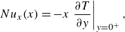 \begin{equation} Nu_x(x) = -x \left .\frac {\partial T}{\partial y}\right |_{y=0^+} ,\end{equation}
with that of Rahman & Tafti (Reference Rahman and Tafti2020a
). Here, we only compare $Nu_x$
on the top plate surface; it is the same on the bottom surface by symmetry. We also compare the Blasius boundary layer solution (Incropera et al. Reference Incropera, DeWitt, Bergman and Lavine2006)
$Nu_x$
on the top plate surface; it is the same on the bottom surface by symmetry. We also compare the Blasius boundary layer solution (Incropera et al. Reference Incropera, DeWitt, Bergman and Lavine2006)
 \begin{equation} Nu_x = 0.332Re_x^{1/2}Pr^{1/3}. \end{equation}
The simulated $Nu_x$
is larger than the Blasius result, especially near the trailing edge. The Blasius assumption of a semi-infinite plate shows the strongest deviation from the finite plate here. For the finite plate only,
$Nu_x$
is larger than the Blasius result, especially near the trailing edge. The Blasius assumption of a semi-infinite plate shows the strongest deviation from the finite plate here. For the finite plate only, $Nu_x$
diverges at the trailing edge, as discussed by Dennis & Smith (Reference Dennis and Smith1966) and Rahman & Tafti (Reference Rahman and Tafti2020a
).
$Nu_x$
diverges at the trailing edge, as discussed by Dennis & Smith (Reference Dennis and Smith1966) and Rahman & Tafti (Reference Rahman and Tafti2020a
).
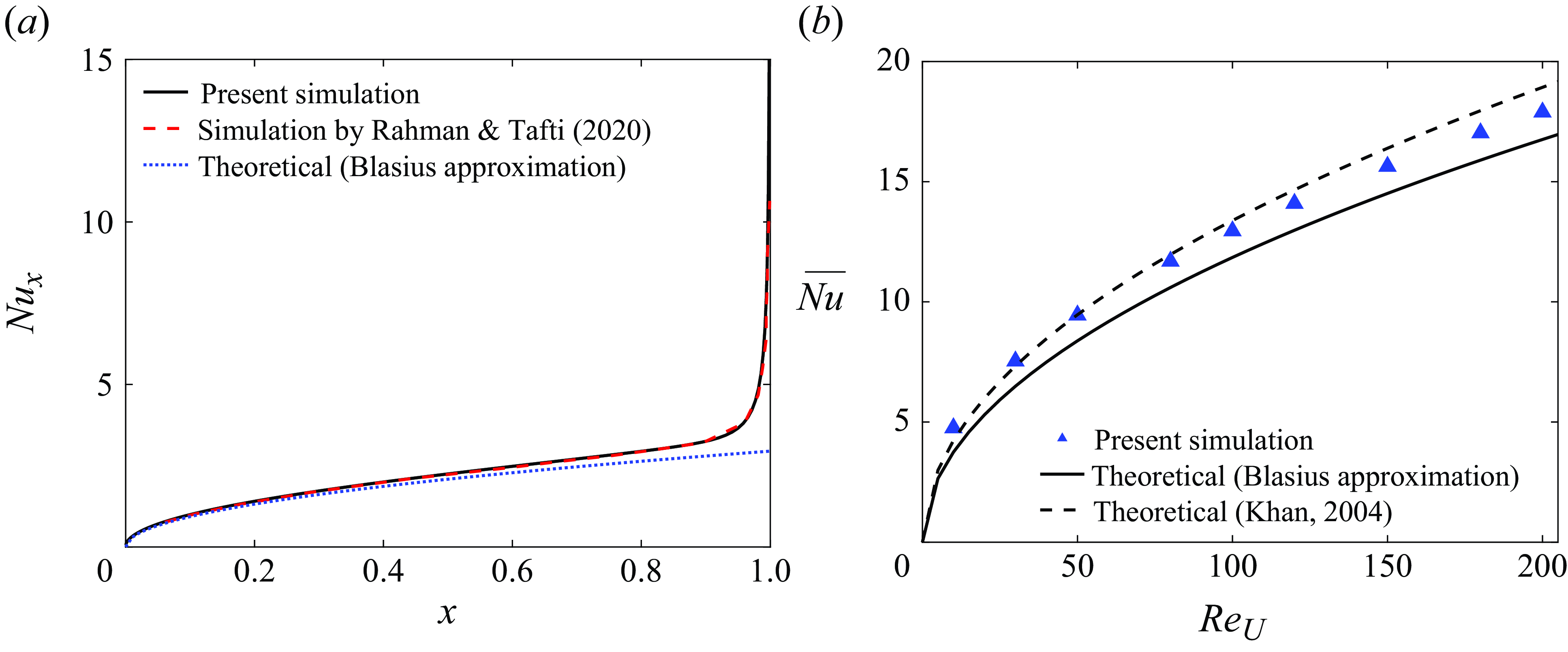
Figure 22. For a stationary plate in the horizontal oncoming flow ( $\gamma =0^\circ$
), (a) the local Nusselt number
$\gamma =0^\circ$
), (a) the local Nusselt number ${Nu}_x$
compared with (Rahman & Tafti Reference Rahman and Tafti2020a
, figure 6) and the Blasius approximation, and (b) the global Nusselt number compared with the Blasius approximation and a different theoretical approximation of Khan (Reference Khan2004).
${Nu}_x$
compared with (Rahman & Tafti Reference Rahman and Tafti2020a
, figure 6) and the Blasius approximation, and (b) the global Nusselt number compared with the Blasius approximation and a different theoretical approximation of Khan (Reference Khan2004).
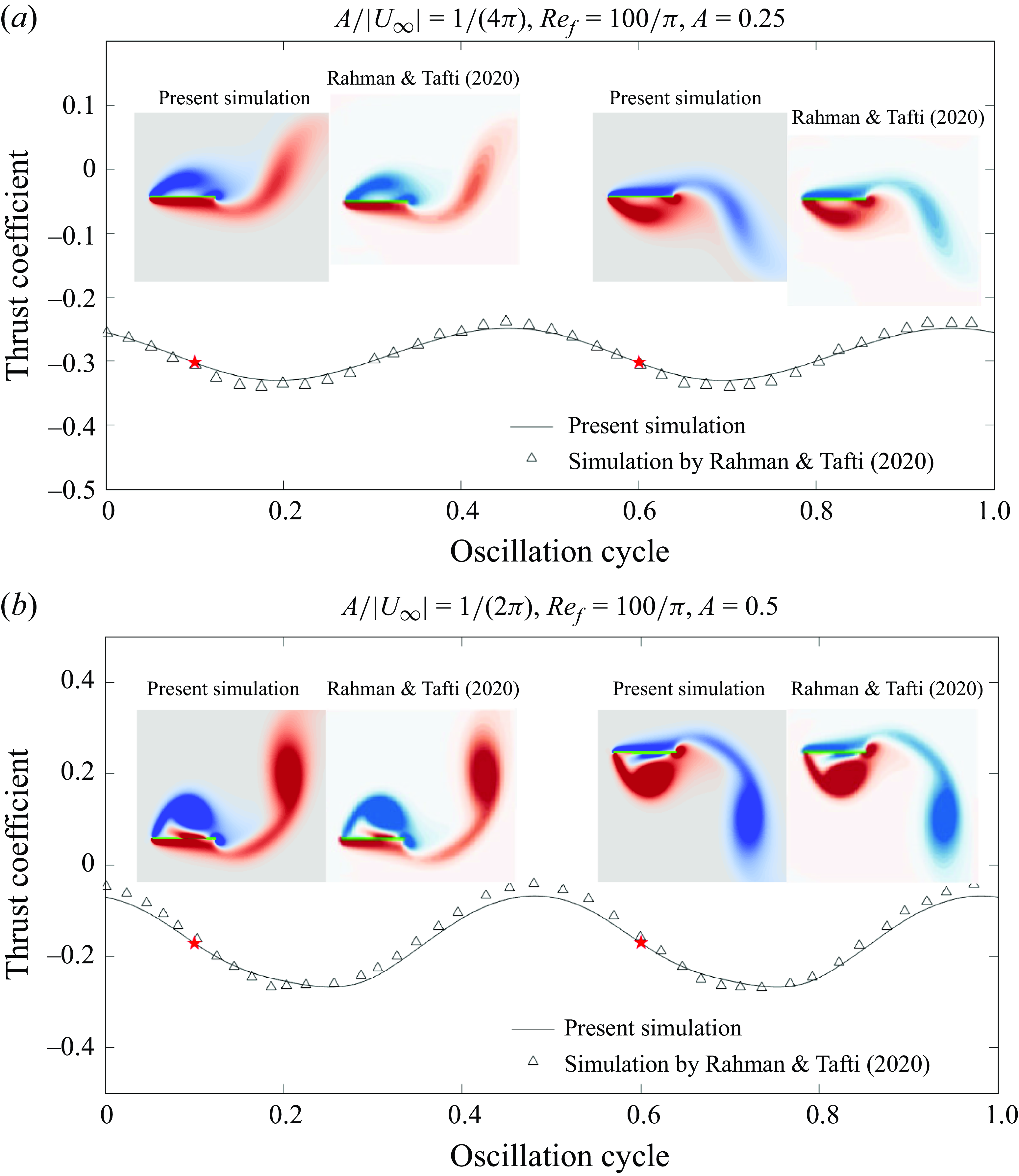
Figure 23. Comparison between the present numerical method and the results from Rahman & Tafti (Reference Rahman and Tafti2020b
) for a vertically oscillating plate ( $\alpha =90^\circ$
) in a horizontal oncoming flow (
$\alpha =90^\circ$
) in a horizontal oncoming flow ( $\gamma =0^\circ$
) with
$\gamma =0^\circ$
) with $Re_U=100$
. The black curve (the present simulation) and the triangles (the results of Rahman & Tafti (Reference Rahman and Tafti2020b
)) in each panel show the histories of the thrust coefficient during one oscillation cycle, defined as
$Re_U=100$
. The black curve (the present simulation) and the triangles (the results of Rahman & Tafti (Reference Rahman and Tafti2020b
)) in each panel show the histories of the thrust coefficient during one oscillation cycle, defined as $F_x/({1}/{2}|\boldsymbol{U}_{\infty }|^2)$
, with
$F_x/({1}/{2}|\boldsymbol{U}_{\infty }|^2)$
, with $F_x$
computed by(5.1). The stars on the curve mark the beginning and the end of upstroke, respectively, with the corresponding vorticity fields compared above the stars in each panel.
$F_x$
computed by(5.1). The stars on the curve mark the beginning and the end of upstroke, respectively, with the corresponding vorticity fields compared above the stars in each panel.
We show corresponding global Nusselt number results in figure 22(b). The symbols show our $\overline {Nu}$
(2.8) at several
$\overline {Nu}$
(2.8) at several $Re_U$
. The simulation results are compared with the Blasius solution (Incropera et al. Reference Incropera, DeWitt, Bergman and Lavine2006)
$Re_U$
. The simulation results are compared with the Blasius solution (Incropera et al. Reference Incropera, DeWitt, Bergman and Lavine2006)
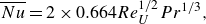 \begin{equation} \overline {Nu} = 2\times 0.664Re_U^{1/2}Pr^{1/3}, \end{equation}
and the theoretical model of Khan (Reference Khan2004):
 \begin{equation} \overline {Nu} = 2\times 0.750Re_U^{1/2}Pr^{1/3}. \end{equation}
The latter is derived for an elliptic body in a uniform oncoming flow. A boundary layer equation is used on the body surface and potential flow is assumed outside the boundary layer. Equation (C4) is obtained in the flat plate limit, i.e. taking the ratio of the minor and major ellipse axes to zero. In equations (C2) and (C4), the factor 2 on the right-hand sides is because both sides of the plate are considered. Similar to the local Nusselt number, the simulated $\overline {Nu}$
is larger than the Blasius approximation. Better agreement is seen between our simulation and (C4), mainly at lower
$\overline {Nu}$
is larger than the Blasius approximation. Better agreement is seen between our simulation and (C4), mainly at lower $Re_U$
.
$Re_U$
.
For two examples of an oscillating plate, we validate our flow simulations with results in Rahman & Tafti (Reference Rahman and Tafti2020b
) in figure 23. Good agreement is seen in the thrust coefficient ( $F_x/({1}/{2}|\boldsymbol{U}_{\infty }|^2)$
with
$F_x/({1}/{2}|\boldsymbol{U}_{\infty }|^2)$
with $F_x$
in (5.1)) over one oscillation cycle and The vorticity fields at the beginning and the end of upstroke (marked with red stars).
$F_x$
in (5.1)) over one oscillation cycle and The vorticity fields at the beginning and the end of upstroke (marked with red stars).
Appendix D. Vorticity strength
In this appendix, we show how the vorticity strength varies with the plate’s orientation, oscillation direction, frequency and amplitude. We define the vorticity strength as the integral of the absolute value of the vorticity within a box around the plate (denoted as $\Omega ^b$
), written as
$\Omega ^b$
), written as
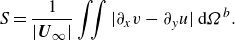 \begin{equation} S = \frac {1}{|\boldsymbol{U}_{\infty }|}\iint |\partial _x v-\partial _y u|\, \textrm{d}\Omega ^b. \end{equation}
Note that $S$
has been rescaled by dividing by
$S$
has been rescaled by dividing by $|\boldsymbol{U}_{\infty }|$
, which corresponds to using the fixed oncoming flow speed
$|\boldsymbol{U}_{\infty }|$
, which corresponds to using the fixed oncoming flow speed $|\boldsymbol{U}^{\star }_{\infty }|$
as the characteristic velocity scale instead of
$|\boldsymbol{U}^{\star }_{\infty }|$
as the characteristic velocity scale instead of $f^\star \ell ^{\star }$
. Then the non-dimensionalisation of vorticity strength does not depend on frequency, so we can compare results with different frequencies, analogous to how we rescaled power in § 5. In figure 25, we show the time-averaged vorticity strength
$f^\star \ell ^{\star }$
. Then the non-dimensionalisation of vorticity strength does not depend on frequency, so we can compare results with different frequencies, analogous to how we rescaled power in § 5. In figure 25, we show the time-averaged vorticity strength $\langle S \rangle$
using boxes of three different sizes:
$\langle S \rangle$
using boxes of three different sizes: $2\times 2$
(panel (a)),
$2\times 2$
(panel (a)), $4\times 4$
(b) and
$4\times 4$
(b) and $6\times 6$
(c). The time average is taken over the same number of cycles as in figure 7. The boxes are chosen to include the plate and surrounding vorticity, and are therefore biased to include more of the downstream than upstream flow. The positions are different for different
$6\times 6$
(c). The time average is taken over the same number of cycles as in figure 7. The boxes are chosen to include the plate and surrounding vorticity, and are therefore biased to include more of the downstream than upstream flow. The positions are different for different $\gamma$
, and are shown in figure 24.
$\gamma$
, and are shown in figure 24.
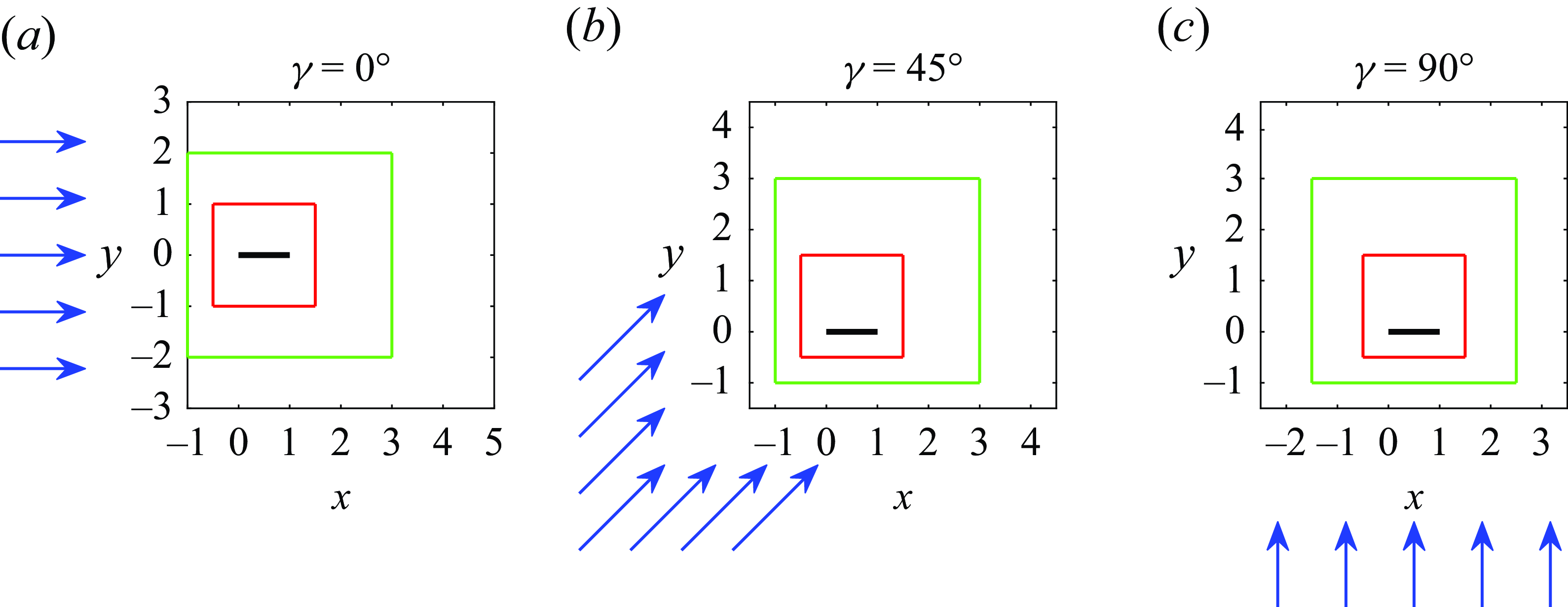
Figure 24. The box’s position relative to the plate (the black line) for (a) $\gamma =0^\circ$
, (b)
$\gamma =0^\circ$
, (b) $\gamma =45^\circ$
and (c)
$\gamma =45^\circ$
and (c) $\gamma =90^\circ$
. In each panel, the boxes in red, green and black have sizes of
$\gamma =90^\circ$
. In each panel, the boxes in red, green and black have sizes of $2\times 2$
,
$2\times 2$
, $4\times 4$
and
$4\times 4$
and $6\times 6$
, respectively. The coordinates of the box vertices are either integers or half-integers. The blue arrows indicate the oncoming flow direction.
$6\times 6$
, respectively. The coordinates of the box vertices are either integers or half-integers. The blue arrows indicate the oncoming flow direction.
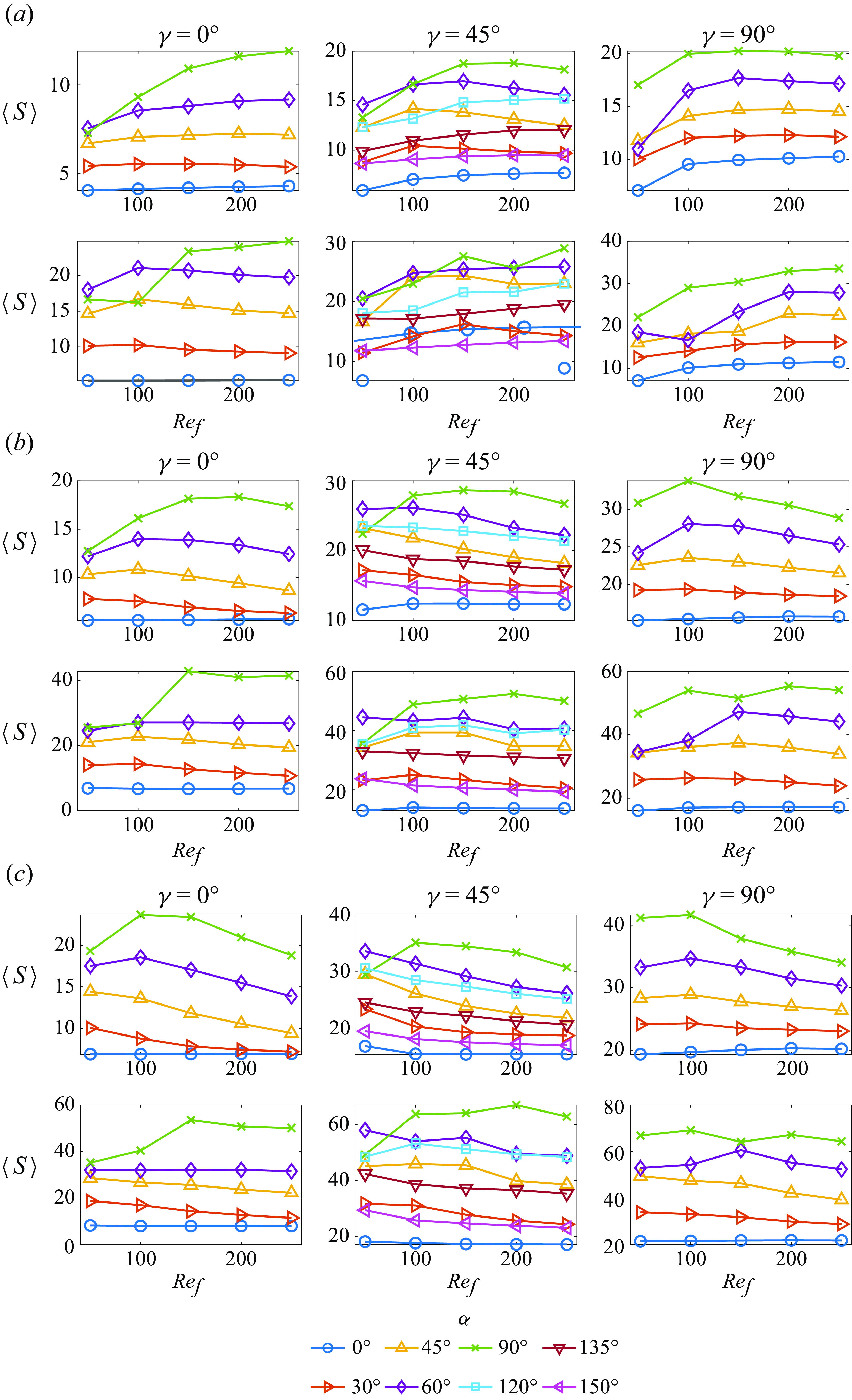
Figure 25. The time-averaged vorticity strength $\langle S \rangle$
computed within a box around the oscillating plate. The box dimensions are (a)
$\langle S \rangle$
computed within a box around the oscillating plate. The box dimensions are (a) $2\times 2$
, (b)
$2\times 2$
, (b) $4\times 4$
and (c)
$4\times 4$
and (c) $6\times 6$
, and shown in figure 24. The first and the second rows correspond to
$6\times 6$
, and shown in figure 24. The first and the second rows correspond to $A/|\boldsymbol{U}_{\infty }|=0.2$
and
$A/|\boldsymbol{U}_{\infty }|=0.2$
and $0.3$
, respectively.
$0.3$
, respectively.
Generally speaking, the overall trends of the time-averaged vorticity $\langle S \rangle$
with respect to
$\langle S \rangle$
with respect to $A/|\boldsymbol{U}_{\infty }|$
,
$A/|\boldsymbol{U}_{\infty }|$
, $\alpha$
and
$\alpha$
and $Re_f$
do not depend very strongly on the box size. It is more straightforward to compare the values of
$Re_f$
do not depend very strongly on the box size. It is more straightforward to compare the values of $\langle S \rangle$
across
$\langle S \rangle$
across $A/|\boldsymbol{U}_{\infty }|$
,
$A/|\boldsymbol{U}_{\infty }|$
, $\alpha$
and
$\alpha$
and $Re_f$
at a given
$Re_f$
at a given $\gamma$
than at different
$\gamma$
than at different $\gamma$
, because the wake vorticity distributions vary with
$\gamma$
, because the wake vorticity distributions vary with $\gamma$
; e.g. the boxes typically include different numbers of vortices at different
$\gamma$
; e.g. the boxes typically include different numbers of vortices at different $\gamma$
.
$\gamma$
.
With the other parameters fixed, $\langle S \rangle$
is larger at
$\langle S \rangle$
is larger at $A/|\boldsymbol{U}_{\infty }|=0.3$
(bottom rows) than
$A/|\boldsymbol{U}_{\infty }|=0.3$
(bottom rows) than $A/|\boldsymbol{U}_{\infty }|=0.2$
(top rows), since stronger vortices are generated at higher oscillation velocity. In most cases,
$A/|\boldsymbol{U}_{\infty }|=0.2$
(top rows), since stronger vortices are generated at higher oscillation velocity. In most cases, $\langle S \rangle$
is larger for more transverse oscillation, i.e.
$\langle S \rangle$
is larger for more transverse oscillation, i.e. $\alpha$
closer to
$\alpha$
closer to $90^\circ$
. Also at
$90^\circ$
. Also at $\gamma =45^\circ$
,
$\gamma =45^\circ$
, $\langle S \rangle$
is larger when the plate oscillates more along the flow (
$\langle S \rangle$
is larger when the plate oscillates more along the flow ( $\alpha \lt 90^\circ$
) than across the flow (
$\alpha \lt 90^\circ$
) than across the flow ( $\alpha \gt 90^\circ$
).
$\alpha \gt 90^\circ$
).
With $A/|\boldsymbol{U}_{\infty }|$
and
$A/|\boldsymbol{U}_{\infty }|$
and $\alpha$
fixed, the vorticity strength
$\alpha$
fixed, the vorticity strength $\langle S \rangle$
does not vary much with
$\langle S \rangle$
does not vary much with $Re_f$
in most cases, as indicated by many flat curves in figure 25. However, a sudden change of
$Re_f$
in most cases, as indicated by many flat curves in figure 25. However, a sudden change of $\langle S \rangle$
as
$\langle S \rangle$
as $Re_f$
increases is also observed in several cases. Those jumps are typically associated with a change in the vortex dynamics. Specifically, the cases with more enhanced vortex grouping have stronger vorticity near the plate because vorticity grouping helps trap the vortices near the plate.
$Re_f$
increases is also observed in several cases. Those jumps are typically associated with a change in the vortex dynamics. Specifically, the cases with more enhanced vortex grouping have stronger vorticity near the plate because vorticity grouping helps trap the vortices near the plate.
In summary, $\langle S \rangle$
varies similarly to the global Nusselt number
$\langle S \rangle$
varies similarly to the global Nusselt number $\langle \overline {Nu} \rangle$
across parameters space, so the strength of shed vorticity is a strong indicator of the global heat transfer. We now discuss the changes in the vortex dynamics that occur as
$\langle \overline {Nu} \rangle$
across parameters space, so the strength of shed vorticity is a strong indicator of the global heat transfer. We now discuss the changes in the vortex dynamics that occur as $\langle S \rangle$
increases from
$\langle S \rangle$
increases from $Re_f = 50$
to
$Re_f = 50$
to $100$
.
$100$
.
At $\gamma =0^\circ$
,
$\gamma =0^\circ$
, $\langle S \rangle$
with
$\langle S \rangle$
with $\alpha =90^\circ$
at
$\alpha =90^\circ$
at $Re_f=50$
and
$Re_f=50$
and $100$
is lower than that at higher
$100$
is lower than that at higher $Re_f$
, as shown by the green curve of the first panel in each row (except the green curve of the upper left subpanel in panel (c)). At
$Re_f$
, as shown by the green curve of the first panel in each row (except the green curve of the upper left subpanel in panel (c)). At $A/|\boldsymbol{U}_{\infty }|=0.2$
, no vortex grouping occurs at
$A/|\boldsymbol{U}_{\infty }|=0.2$
, no vortex grouping occurs at $Re_f=50$
and
$Re_f=50$
and $Re_f=100$
(and the vortices shed display up–down symmetry as in figure 11
a), while the positive vortices merge at the plate’s left edge every cycle at
$Re_f=100$
(and the vortices shed display up–down symmetry as in figure 11
a), while the positive vortices merge at the plate’s left edge every cycle at $Re_f\gt 100$
(with the up–down symmetry broken as shown in figure 11
b). Consequently, the cases at
$Re_f\gt 100$
(with the up–down symmetry broken as shown in figure 11
b). Consequently, the cases at $Re_f\gt 100$
have stronger vorticity near the plate. At
$Re_f\gt 100$
have stronger vorticity near the plate. At $A/|\boldsymbol{U}_{\infty }|=0.3$
, the positive vortices merge every cycle at the plate’s left edge at
$A/|\boldsymbol{U}_{\infty }|=0.3$
, the positive vortices merge every cycle at the plate’s left edge at $Re_f=50$
and
$Re_f=50$
and $Re_f=100$
as in figure 11(b), but the cases at
$Re_f=100$
as in figure 11(b), but the cases at $Re_f\gt 100$
become non-periodic, with not only the positive vortices but also the negative vortices grouping at the left edge for many cycles, and the resulting vorticity strength is much larger than for
$Re_f\gt 100$
become non-periodic, with not only the positive vortices but also the negative vortices grouping at the left edge for many cycles, and the resulting vorticity strength is much larger than for $Re_f=50$
and
$Re_f=50$
and $Re_f=100$
.
$Re_f=100$
.
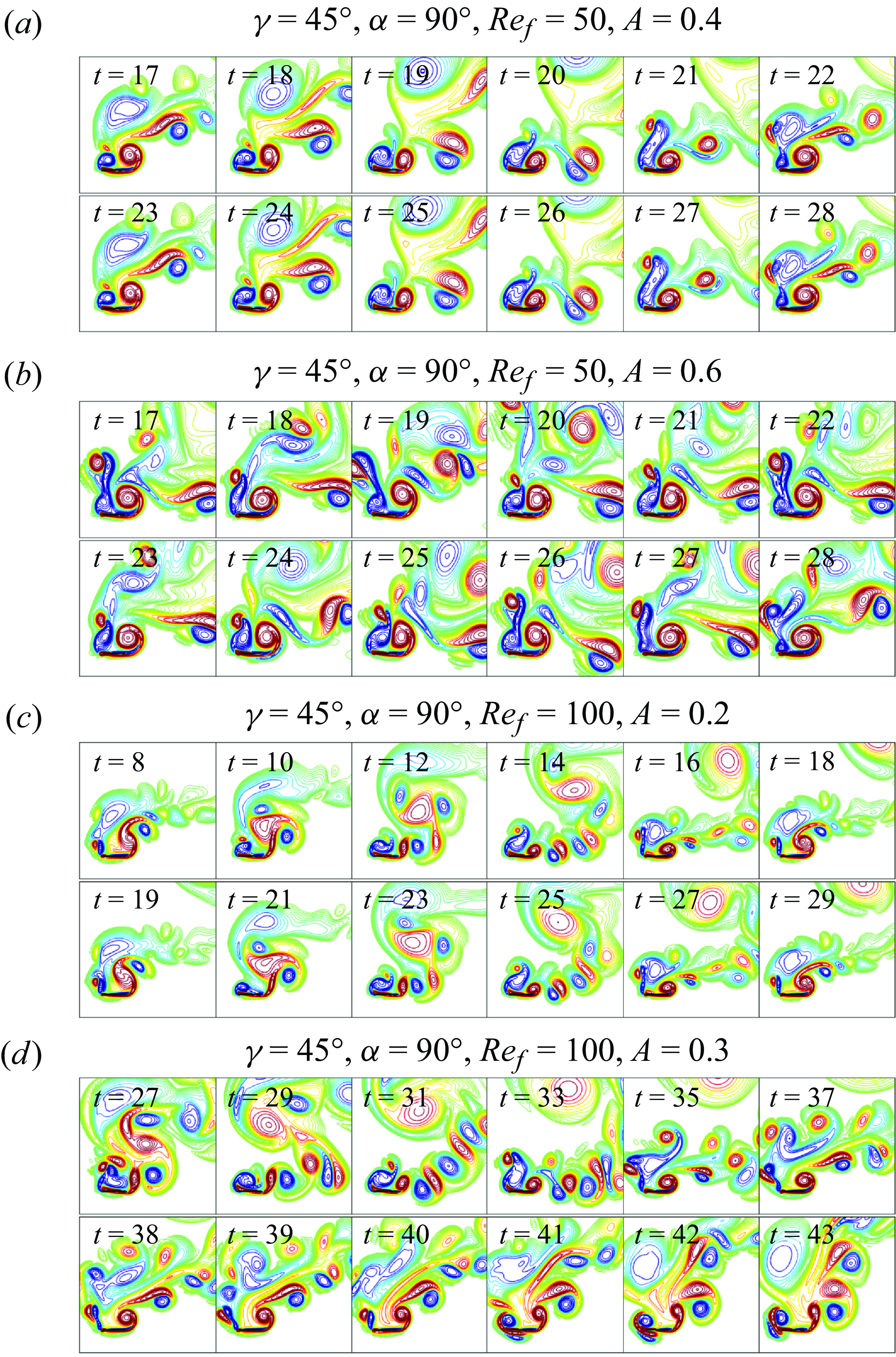
Figure 26. Changes in the vortex dynamics from $Re_f=50$
((a) to (b)) to
$Re_f=50$
((a) to (b)) to $Re_f=100$
((c) and (d)) with
$Re_f=100$
((c) and (d)) with $\gamma =45^\circ$
and
$\gamma =45^\circ$
and $\alpha =90^\circ$
.
$\alpha =90^\circ$
.
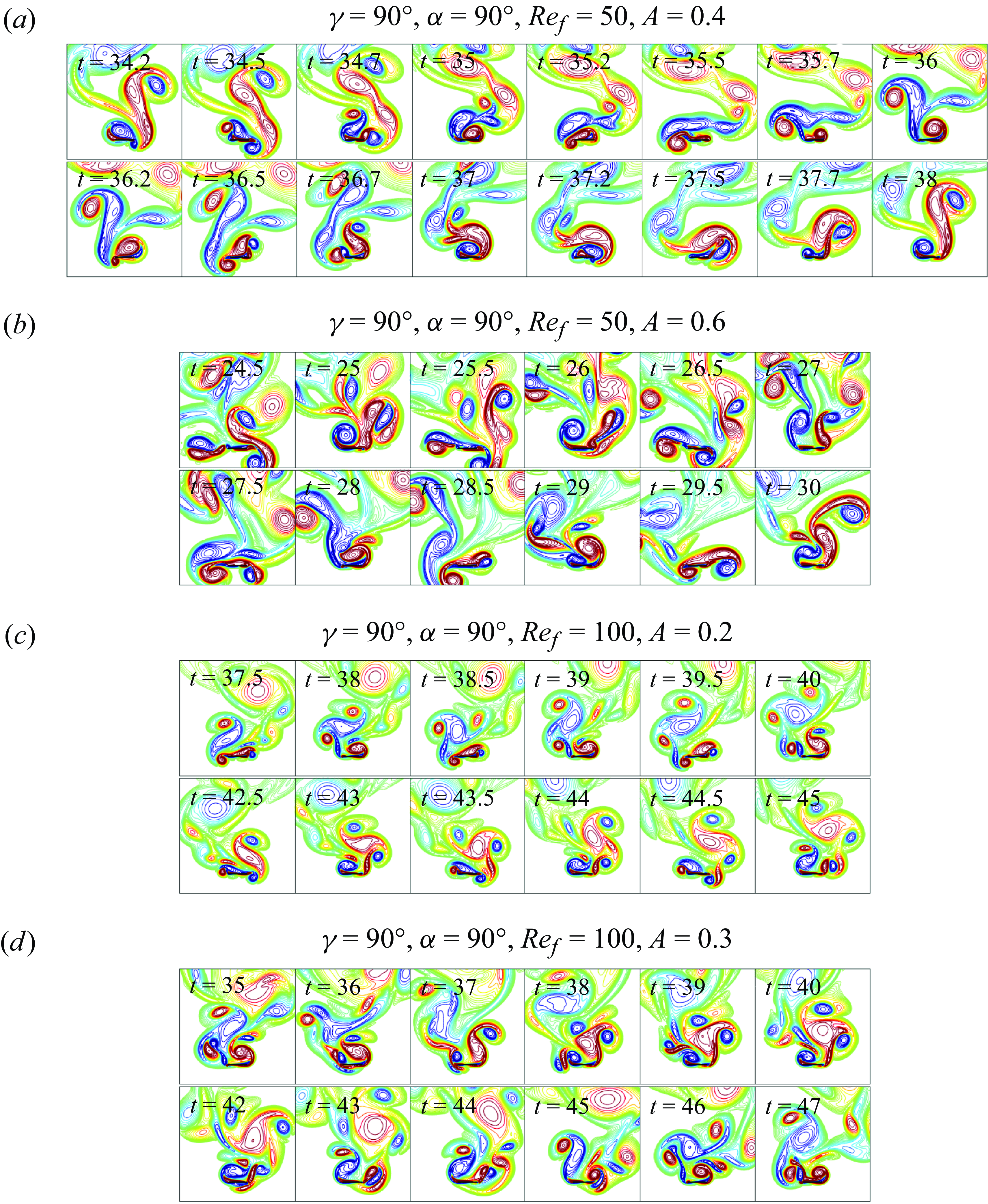
Figure 27. Change of vortex dynamics from $Re_f=50$
((a) to (b)) to
$Re_f=50$
((a) to (b)) to $Re_f=100$
((c) and (d)) with
$Re_f=100$
((c) and (d)) with $\gamma =90^\circ$
and
$\gamma =90^\circ$
and $\alpha =90^\circ$
.
$\alpha =90^\circ$
.
A jump in $\langle S \rangle$
is also found with
$\langle S \rangle$
is also found with $\gamma =45^\circ$
and
$\gamma =45^\circ$
and $\alpha =90^\circ$
as
$\alpha =90^\circ$
as $Re_f$
increases from 50 to 100 at both
$Re_f$
increases from 50 to 100 at both $A/|\boldsymbol{U}_{\infty }|=0.2$
and
$A/|\boldsymbol{U}_{\infty }|=0.2$
and $0.3$
. As shown in panels (a) and (c) of figure 26, for
$0.3$
. As shown in panels (a) and (c) of figure 26, for $\gamma =45^\circ$
at
$\gamma =45^\circ$
at $A/|\boldsymbol{U}_{\infty }|=0.2$
, the negative vortices merge at the plate’s left edge every 6 cycles of oscillations and there is no vortex grouping at the right edge at
$A/|\boldsymbol{U}_{\infty }|=0.2$
, the negative vortices merge at the plate’s left edge every 6 cycles of oscillations and there is no vortex grouping at the right edge at $Re_f=50$
, while vortex grouping at
$Re_f=50$
, while vortex grouping at $Re_f=100$
is enhanced with the merging of positive and negative vortices at the two edges alternately every 11 cycles of oscillations. (Note that in (a) and (c) the two rows are similar, indicating that the two cases are almost periodic over several cycles). Panels (b) and (d) of figure 26 show the comparison between
$Re_f=100$
is enhanced with the merging of positive and negative vortices at the two edges alternately every 11 cycles of oscillations. (Note that in (a) and (c) the two rows are similar, indicating that the two cases are almost periodic over several cycles). Panels (b) and (d) of figure 26 show the comparison between $Re_f=50$
and
$Re_f=50$
and $100$
for
$100$
for $\gamma =45^\circ$
at
$\gamma =45^\circ$
at $A/|\boldsymbol{U}_{\infty }|=0.3$
. Both cases are non-periodic. No vortex grouping occurs at
$A/|\boldsymbol{U}_{\infty }|=0.3$
. Both cases are non-periodic. No vortex grouping occurs at $Re_f=50$
whereas the negative vortices group at the left edge (as shown by the first row of panel (d)) and the positive vortices tend to group loosely at the right edge at
$Re_f=50$
whereas the negative vortices group at the left edge (as shown by the first row of panel (d)) and the positive vortices tend to group loosely at the right edge at $Re_f=100$
(as shown by the second row of panel (d)).
$Re_f=100$
(as shown by the second row of panel (d)).
We also observe that the vorticity strength suddenly increases from $Re_f=50$
to
$Re_f=50$
to $100$
for
$100$
for $\gamma =90^\circ$
and
$\gamma =90^\circ$
and $\alpha =90^\circ$
at both
$\alpha =90^\circ$
at both $A/|\boldsymbol{U}_{\infty }|=0.2$
and
$A/|\boldsymbol{U}_{\infty }|=0.2$
and $0.3$
, and
$0.3$
, and $\alpha =60^\circ$
at
$\alpha =60^\circ$
at $A/|\boldsymbol{U}_{\infty }|=0.2$
. Similarly, the stronger vorticity at
$A/|\boldsymbol{U}_{\infty }|=0.2$
. Similarly, the stronger vorticity at $Re_f=100$
results from more enhanced vortex grouping at
$Re_f=100$
results from more enhanced vortex grouping at $Re_f=100$
. Here, we only show the cases with
$Re_f=100$
. Here, we only show the cases with $\alpha =90^\circ$
for simplicity but the situation with
$\alpha =90^\circ$
for simplicity but the situation with $\alpha =60^\circ$
is similar. As shown in figure 27(a), at
$\alpha =60^\circ$
is similar. As shown in figure 27(a), at $Re_f=50$
and
$Re_f=50$
and $A/|\boldsymbol{U}_{\infty }|=0.2$
, the negative and positive vortices from two consecutive cycles tend to merge at the two edges alternately but they ungroup quickly once shed from the plate. However, at
$A/|\boldsymbol{U}_{\infty }|=0.2$
, the negative and positive vortices from two consecutive cycles tend to merge at the two edges alternately but they ungroup quickly once shed from the plate. However, at $Re_f=100$
, as shown in figure 27(c), compact vortex groups are formed at the two edges by merging vortices from several cycles (note that the second row is the mirror image of the first row), resulting in stronger vorticity near the plate. For the cases with
$Re_f=100$
, as shown in figure 27(c), compact vortex groups are formed at the two edges by merging vortices from several cycles (note that the second row is the mirror image of the first row), resulting in stronger vorticity near the plate. For the cases with $A/|\boldsymbol{U}_{\infty }|=0.3$
shown in panels (b) and (d), although they are non-periodic with an irregular vortex dynamics, positive and negative vortex grouping are observed to occur at the two edges at
$A/|\boldsymbol{U}_{\infty }|=0.3$
shown in panels (b) and (d), although they are non-periodic with an irregular vortex dynamics, positive and negative vortex grouping are observed to occur at the two edges at $Re_f=100$
while no vortex grouping occurs near the plate at
$Re_f=100$
while no vortex grouping occurs near the plate at $Re_f=50$
.
$Re_f=50$
.
In summary, stronger vorticity typically occurs as $Re_f$
increases from 50 to 100 because there is stronger vortex grouping near the plate.
$Re_f$
increases from 50 to 100 because there is stronger vortex grouping near the plate.
Appendix E. Long-time-averaged local Nusselt number at
$\boldsymbol{\gamma} =\boldsymbol{45}^{\boldsymbol{\circ}}$
and
$\boldsymbol{\gamma} = \boldsymbol{90}^{\boldsymbol{\circ}}$


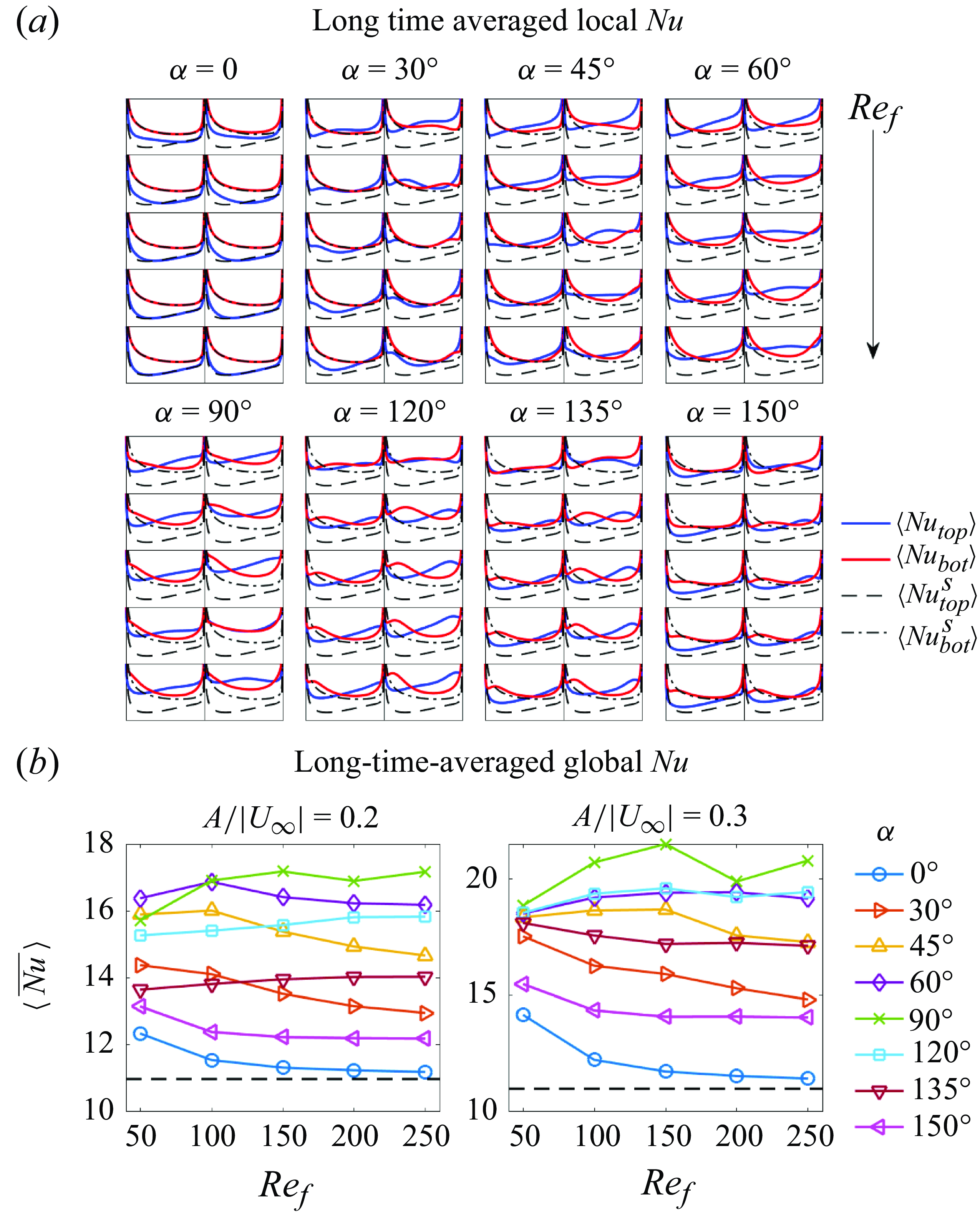
Figure 28. (a) The long-time-averaged local $Nu$
and (b) the time-averaged global
$Nu$
and (b) the time-averaged global $Nu$
at
$Nu$
at $\gamma =45^\circ$
. Note that the number of cycles taken to compute the time average is the same in (a) and (b). The graphs in (a) are arranged in eight columns, one for each
$\gamma =45^\circ$
. Note that the number of cycles taken to compute the time average is the same in (a) and (b). The graphs in (a) are arranged in eight columns, one for each $\alpha$
, and five rows, one for each
$\alpha$
, and five rows, one for each $Re_f$
from 50 to 250, increasing downward. Pairs of subpanels are shown in each column, corresponding to
$Re_f$
from 50 to 250, increasing downward. Pairs of subpanels are shown in each column, corresponding to $A/|\boldsymbol{U}_{\infty }| =0.2$
and 0.3 on the left and right, respectively. Here,
$A/|\boldsymbol{U}_{\infty }| =0.2$
and 0.3 on the left and right, respectively. Here, $\langle Nu_{{top}}^s \rangle$
(black dashed curve) and
$\langle Nu_{{top}}^s \rangle$
(black dashed curve) and $\langle Nu_{{bot}}^s \rangle$
(black dash-dotted curve) in (a) denote the time-averaged local
$\langle Nu_{{bot}}^s \rangle$
(black dash-dotted curve) in (a) denote the time-averaged local $Nu$
on the top and bottom walls of the non-oscillating plate, respectively.
$Nu$
on the top and bottom walls of the non-oscillating plate, respectively.

Figure 29. (a) The long-time-averaged local $Nu$
and (b) the time-averaged global
$Nu$
and (b) the time-averaged global $Nu$
at
$Nu$
at $\gamma =90^\circ$
. Note that the number of cycles taken to compute the time average is the same in (a) and (b). The graphs in (a) are arranged in five columns, one for each
$\gamma =90^\circ$
. Note that the number of cycles taken to compute the time average is the same in (a) and (b). The graphs in (a) are arranged in five columns, one for each $\alpha$
, and five rows, one for each
$\alpha$
, and five rows, one for each $Re_f$
from 50 to 250, increasing downward. Pairs of subpanels are shown in each column, corresponding to
$Re_f$
from 50 to 250, increasing downward. Pairs of subpanels are shown in each column, corresponding to $A/|\boldsymbol{U}_{\infty }| =0.2$
and 0.3 on the left and right, respectively. Here,
$A/|\boldsymbol{U}_{\infty }| =0.2$
and 0.3 on the left and right, respectively. Here, $\langle Nu_{{top}}^s \rangle$
(black dashed curve) and
$\langle Nu_{{top}}^s \rangle$
(black dashed curve) and $\langle Nu_{{bot}}^s \rangle$
(black dash-dotted curve) in (a) denote the time-averaged local
$\langle Nu_{{bot}}^s \rangle$
(black dash-dotted curve) in (a) denote the time-averaged local $Nu$
on the top and bottom walls of the non-oscillating plate, respectively.
$Nu$
on the top and bottom walls of the non-oscillating plate, respectively.
In this appendix, we show the time-averaged local Nusselt number at $\gamma =45^\circ$
and
$\gamma =45^\circ$
and $\gamma =90^\circ$
as a supplement to the cycle-averaged local quantities discussed in §§ 4.2.2 and 4.2.3. The time interval used to compute the averaged local
$\gamma =90^\circ$
as a supplement to the cycle-averaged local quantities discussed in §§ 4.2.2 and 4.2.3. The time interval used to compute the averaged local $Nu$
is the same as in figure 7, and the time-averaged global
$Nu$
is the same as in figure 7, and the time-averaged global $Nu$
is repeated as the second panels in figures 28 and 29 for convenience.
$Nu$
is repeated as the second panels in figures 28 and 29 for convenience.
Figure 28(a) shows the time-averaged local $Nu$
at
$Nu$
at $\gamma =45^\circ$
. Note that the subpanels share the same
$\gamma =45^\circ$
. Note that the subpanels share the same $y$
axis, and the values of the non-oscillating plate (black curves) are given as reference values. As the vortex wake is mainly behind the top wall,
$y$
axis, and the values of the non-oscillating plate (black curves) are given as reference values. As the vortex wake is mainly behind the top wall, $\langle Nu_{{top}} \rangle$
is improved more than
$\langle Nu_{{top}} \rangle$
is improved more than $\langle Nu_{{bot}}\rangle$
. The improvement is more pronounced at the higher
$\langle Nu_{{bot}}\rangle$
. The improvement is more pronounced at the higher $A/|\boldsymbol{U}_{\infty }| =0.3$
(the right panels of each column) and when the oscillation is more transverse with
$A/|\boldsymbol{U}_{\infty }| =0.3$
(the right panels of each column) and when the oscillation is more transverse with $\alpha$
closer to
$\alpha$
closer to $90^\circ$
, which is consistent with the variation of
$90^\circ$
, which is consistent with the variation of $\langle \overline {Nu}\rangle$
(i.e. the space average of the local
$\langle \overline {Nu}\rangle$
(i.e. the space average of the local $Nu$
) with
$Nu$
) with $A/|\boldsymbol{U}_{\infty }|$
and
$A/|\boldsymbol{U}_{\infty }|$
and $\alpha$
in panel (b).
$\alpha$
in panel (b).
The effect of $Re_f$
is more complicated. When the plate oscillates in plane (
$Re_f$
is more complicated. When the plate oscillates in plane ( $\alpha =0^\circ$
),
$\alpha =0^\circ$
), $\langle Nu_{{top}} \rangle$
is improved slightly at the left edge but the improvement diminishes as
$\langle Nu_{{top}} \rangle$
is improved slightly at the left edge but the improvement diminishes as $Re_f$
increases, while
$Re_f$
increases, while $\langle Nu_{{bot}} \rangle$
is almost the same as the non-oscillating plate. Consequently, we see
$\langle Nu_{{bot}} \rangle$
is almost the same as the non-oscillating plate. Consequently, we see $\langle \overline {Nu}\rangle$
with
$\langle \overline {Nu}\rangle$
with $\alpha =0^\circ$
decreases with
$\alpha =0^\circ$
decreases with $Re_f$
and
$Re_f$
and $\langle \overline {Nu}\rangle$
with
$\langle \overline {Nu}\rangle$
with $\alpha =30^\circ$
and
$\alpha =30^\circ$
and $\alpha =150^\circ$
also decrease monotonically with
$\alpha =150^\circ$
also decrease monotonically with $Re_f$
, but the local
$Re_f$
, but the local $Nu$
for the two cases is different. The case of
$Nu$
for the two cases is different. The case of $\alpha =30^\circ$
is more like
$\alpha =30^\circ$
is more like $\alpha =0^\circ$
. As
$\alpha =0^\circ$
. As $Re_f$
increases, the vortices become smaller, making the enhancement of
$Re_f$
increases, the vortices become smaller, making the enhancement of $\langle Nu_{{top}} \rangle$
near the left edge less significant;
$\langle Nu_{{top}} \rangle$
near the left edge less significant; $\langle Nu_{{bot}} \rangle$
near the right edge is also improved with
$\langle Nu_{{bot}} \rangle$
near the right edge is also improved with $\alpha =30^\circ$
at
$\alpha =30^\circ$
at $A/|\boldsymbol{U}_{\infty }| =0.3$
. Similarly, the improvement becomes less pronounced as
$A/|\boldsymbol{U}_{\infty }| =0.3$
. Similarly, the improvement becomes less pronounced as $Re_f$
increases. The case of
$Re_f$
increases. The case of $\alpha =150^\circ$
has the same vertical oscillation velocity as
$\alpha =150^\circ$
has the same vertical oscillation velocity as $\alpha =30^\circ$
but the horizontal oscillation is opposite. Both
$\alpha =30^\circ$
but the horizontal oscillation is opposite. Both $\langle Nu_{{top}} \rangle$
and
$\langle Nu_{{top}} \rangle$
and $\langle Nu_{{bot}} \rangle$
at
$\langle Nu_{{bot}} \rangle$
at $\alpha =150^\circ$
are improved over a broader range of the plate, each with a dip located near the right and left edges, respectively. This pattern of local
$\alpha =150^\circ$
are improved over a broader range of the plate, each with a dip located near the right and left edges, respectively. This pattern of local $Nu$
distribution is also observed in the other cases with
$Nu$
distribution is also observed in the other cases with $\alpha \gt 90^\circ$
, i.e.
$\alpha \gt 90^\circ$
, i.e. $\alpha =120^\circ$
and
$\alpha =120^\circ$
and $135^\circ$
. Furthermore, the dips move closer to the edges and the improved regions seem to shrink as
$135^\circ$
. Furthermore, the dips move closer to the edges and the improved regions seem to shrink as $Re_f$
increases. However, only at
$Re_f$
increases. However, only at $\alpha =150^\circ$
, we see that the local
$\alpha =150^\circ$
, we see that the local $Nu$
is less enhanced as
$Nu$
is less enhanced as $Re_f$
increases, while the variation at
$Re_f$
increases, while the variation at $\alpha =120^\circ$
and
$\alpha =120^\circ$
and $135^\circ$
is more complicated. As shown in panel (b), the global
$135^\circ$
is more complicated. As shown in panel (b), the global $Nu$
at
$Nu$
at $\alpha =120^\circ$
and
$\alpha =120^\circ$
and $135^\circ$
slightly increase with increasing
$135^\circ$
slightly increase with increasing $Re_f$
at
$Re_f$
at $A/|\boldsymbol{U}_{\infty }|=0.2$
and vary non-monotonically with
$A/|\boldsymbol{U}_{\infty }|=0.2$
and vary non-monotonically with $Re_f$
at
$Re_f$
at $A/|\boldsymbol{U}_{\infty }|=0.3$
. For the other cases,
$A/|\boldsymbol{U}_{\infty }|=0.3$
. For the other cases, $\alpha =45^\circ$
–
$\alpha =45^\circ$
– $90^\circ$
, significant improvement is observed in
$90^\circ$
, significant improvement is observed in $\langle Nu_{{top}} \rangle$
over a broad range of the plate while the enhancement of
$\langle Nu_{{top}} \rangle$
over a broad range of the plate while the enhancement of $\langle Nu_{{bot}} \rangle$
is more significant near the right edge. Monotonic variations of the local and global
$\langle Nu_{{bot}} \rangle$
is more significant near the right edge. Monotonic variations of the local and global $Nu$
with
$Nu$
with $Re_f$
are not seen in this range of
$Re_f$
are not seen in this range of $\alpha$
. Typically, strong vortices are generated and complicated interactions between vortices are observed with
$\alpha$
. Typically, strong vortices are generated and complicated interactions between vortices are observed with $\alpha =45^\circ$
to
$\alpha =45^\circ$
to $135^\circ$
, which do not give rise to a simple correlation between heat transfer and
$135^\circ$
, which do not give rise to a simple correlation between heat transfer and $Re_f$
.
$Re_f$
.
The time-averaged local $Nu$
at
$Nu$
at $\gamma =90^\circ$
is shown in figure 29 and has a pattern similar to figure 28. As for
$\gamma =90^\circ$
is shown in figure 29 and has a pattern similar to figure 28. As for $\gamma =90^\circ$
,
$\gamma =90^\circ$
, $\langle Nu_{{top}} \rangle$
is enhanced more than
$\langle Nu_{{top}} \rangle$
is enhanced more than $\langle Nu_{{bot}} \rangle$
, and the enhancement is more significant at larger
$\langle Nu_{{bot}} \rangle$
, and the enhancement is more significant at larger $A/|\boldsymbol{U}_{\infty }|$
and
$A/|\boldsymbol{U}_{\infty }|$
and $\alpha$
closer to
$\alpha$
closer to $90^\circ$
. The distribution of local
$90^\circ$
. The distribution of local $Nu$
is symmetric at
$Nu$
is symmetric at $\alpha =0^\circ$
, with
$\alpha =0^\circ$
, with $\langle Nu_{{top}} \rangle$
improved most significantly at the lowest
$\langle Nu_{{top}} \rangle$
improved most significantly at the lowest $Re_f=50$
. The global
$Re_f=50$
. The global $Nu$
also decreases with
$Nu$
also decreases with $Re_f$
at
$Re_f$
at $\alpha =0^\circ$
. For
$\alpha =0^\circ$
. For $\alpha =30^\circ$
–
$\alpha =30^\circ$
– $60^\circ$
, the distribution of local
$60^\circ$
, the distribution of local $Nu$
is asymmetric. Due to the intense positive vortex group formed at the right edge (as shown in figure 15), the enhancement near the left edge is more significant, usually with a local maximum of
$Nu$
is asymmetric. Due to the intense positive vortex group formed at the right edge (as shown in figure 15), the enhancement near the left edge is more significant, usually with a local maximum of $\langle Nu_{{top}} \rangle$
located near the left edge. As
$\langle Nu_{{top}} \rangle$
located near the left edge. As $Re_f$
increases, the local maximum moves closer to the left edge. An improvement in
$Re_f$
increases, the local maximum moves closer to the left edge. An improvement in $\langle Nu_{{bot}} \rangle$
is also seen at
$\langle Nu_{{bot}} \rangle$
is also seen at $\alpha =30^\circ$
with
$\alpha =30^\circ$
with $A/|\boldsymbol{U}_{\infty }| =0.3$
, and at
$A/|\boldsymbol{U}_{\infty }| =0.3$
, and at $\alpha =45^\circ$
and
$\alpha =45^\circ$
and $60^\circ$
with both
$60^\circ$
with both $A/|\boldsymbol{U}_{\infty }|$
. The enhancement is most significant near the right edge, and the improved area gradually shrinks as
$A/|\boldsymbol{U}_{\infty }|$
. The enhancement is most significant near the right edge, and the improved area gradually shrinks as $Re_f$
increases. However, this shrinkage does not necessarily lead to decreased global heat transfer. As shown in panel (b),
$Re_f$
increases. However, this shrinkage does not necessarily lead to decreased global heat transfer. As shown in panel (b), $\langle \overline {Nu} \rangle$
does not vary much with
$\langle \overline {Nu} \rangle$
does not vary much with $Re_f$
at
$Re_f$
at $\alpha =30^\circ$
and
$\alpha =30^\circ$
and $45^\circ$
, and has non-monotonic variation at
$45^\circ$
, and has non-monotonic variation at $\alpha =60^\circ$
. Finally, at
$\alpha =60^\circ$
. Finally, at $\alpha =90^\circ$
, the local
$\alpha =90^\circ$
, the local $Nu$
becomes more symmetric again because the vortices/vortex groups at the two edges have similar intensities. Here,
$Nu$
becomes more symmetric again because the vortices/vortex groups at the two edges have similar intensities. Here, $\langle Nu_{{top}} \rangle$
has a local maximum in the middle of the plate because the vortices bring the hot fluid toward the two edges alternately. The enhancement at the lowest
$\langle Nu_{{top}} \rangle$
has a local maximum in the middle of the plate because the vortices bring the hot fluid toward the two edges alternately. The enhancement at the lowest $Re_f$
of 50 is the smallest since vortex grouping is less intense than in the other cases, leading to weaker vorticity and thus weaker mixing near the plate (as shown in figure 27 and see our discussion in Appendix D). Beyond
$Re_f$
of 50 is the smallest since vortex grouping is less intense than in the other cases, leading to weaker vorticity and thus weaker mixing near the plate (as shown in figure 27 and see our discussion in Appendix D). Beyond $Re_f=50$
, no significant changes in local
$Re_f=50$
, no significant changes in local $Nu$
are observed as
$Nu$
are observed as $Re_f$
changes. The corresponding global
$Re_f$
changes. The corresponding global $Nu$
also stays at a fairly constant level.
$Nu$
also stays at a fairly constant level.
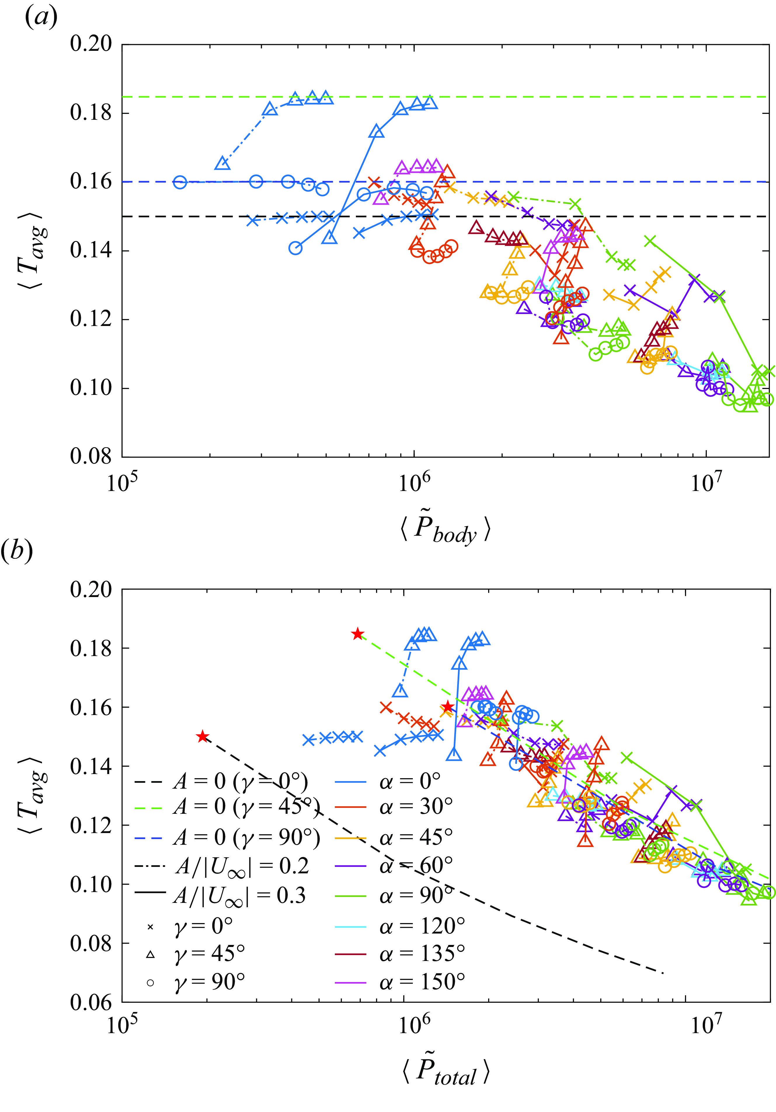
Figure 30. Value of $\langle T_{{avg}} \rangle$
versus the time-averaged power needed to oscillate the plate (a), and the time-averaged total power including the power needed to drive the oncoming flow (b). The three horizontal dashed lines in (a) mark
$\langle T_{{avg}} \rangle$
versus the time-averaged power needed to oscillate the plate (a), and the time-averaged total power including the power needed to drive the oncoming flow (b). The three horizontal dashed lines in (a) mark $\langle T_{{avg}} \rangle$
for the steady plate. The three dashed curves in (b) show
$\langle T_{{avg}} \rangle$
for the steady plate. The three dashed curves in (b) show $\langle T_{{avg}} \rangle$
versus
$\langle T_{{avg}} \rangle$
versus $\langle \tilde {P}_{{total}} \rangle$
for the steady plate. The values with
$\langle \tilde {P}_{{total}} \rangle$
for the steady plate. The values with $Re_U = 100$
are marked with red stars.
$Re_U = 100$
are marked with red stars.
Appendix F. Pareto fronts for the fixed-heat-flux case
In this appendix we present $\langle T_{{avg}} \rangle$
versus the input powers (figure 30) and
$\langle T_{{avg}} \rangle$
versus the input powers (figure 30) and $\max (T_{max })$
versus the input powers (figure 32) for the fixed-heat-flux case. For both figures, a case is Pareto optimal with respect to another case if it lies below and to the left of it. The Pareto optimal cases are those that minimise
$\max (T_{max })$
versus the input powers (figure 32) for the fixed-heat-flux case. For both figures, a case is Pareto optimal with respect to another case if it lies below and to the left of it. The Pareto optimal cases are those that minimise $\langle T_{{avg}} \rangle$
or
$\langle T_{{avg}} \rangle$
or $\max (T_{max })$
at a given input power, or minimise the input power at a given
$\max (T_{max })$
at a given input power, or minimise the input power at a given $\langle T_{{avg}} \rangle$
or
$\langle T_{{avg}} \rangle$
or $\max (T_{max })$
.
$\max (T_{max })$
.
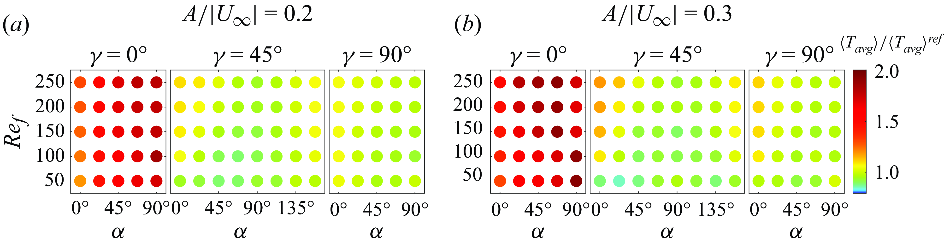
Figure 31. Comparison of $\langle T_{{avg}} \rangle$
between the oscillating and stationary plate at the same total input power. Panels (a) and (b) correspond to
$\langle T_{{avg}} \rangle$
between the oscillating and stationary plate at the same total input power. Panels (a) and (b) correspond to $A/|\boldsymbol{U}_{\infty }|=0.2$
and 0.3, respectively. The different colours of the filled circles in the
$A/|\boldsymbol{U}_{\infty }|=0.2$
and 0.3, respectively. The different colours of the filled circles in the $\alpha$
-
$\alpha$
- $Re_f$
plane correspond to different values of the ratio of
$Re_f$
plane correspond to different values of the ratio of $\langle T_{{avg}} \rangle / \langle T_{{avg}} \rangle ^{{ref}}$
, with
$\langle T_{{avg}} \rangle / \langle T_{{avg}} \rangle ^{{ref}}$
, with $\langle T_{{avg}} \rangle$
and
$\langle T_{{avg}} \rangle$
and $\langle T_{{avg}}\rangle ^{{ref}}$
computed for the oscillating and stationary plate at the same total input power evaluated with equation (5.5).
$\langle T_{{avg}}\rangle ^{{ref}}$
computed for the oscillating and stationary plate at the same total input power evaluated with equation (5.5).
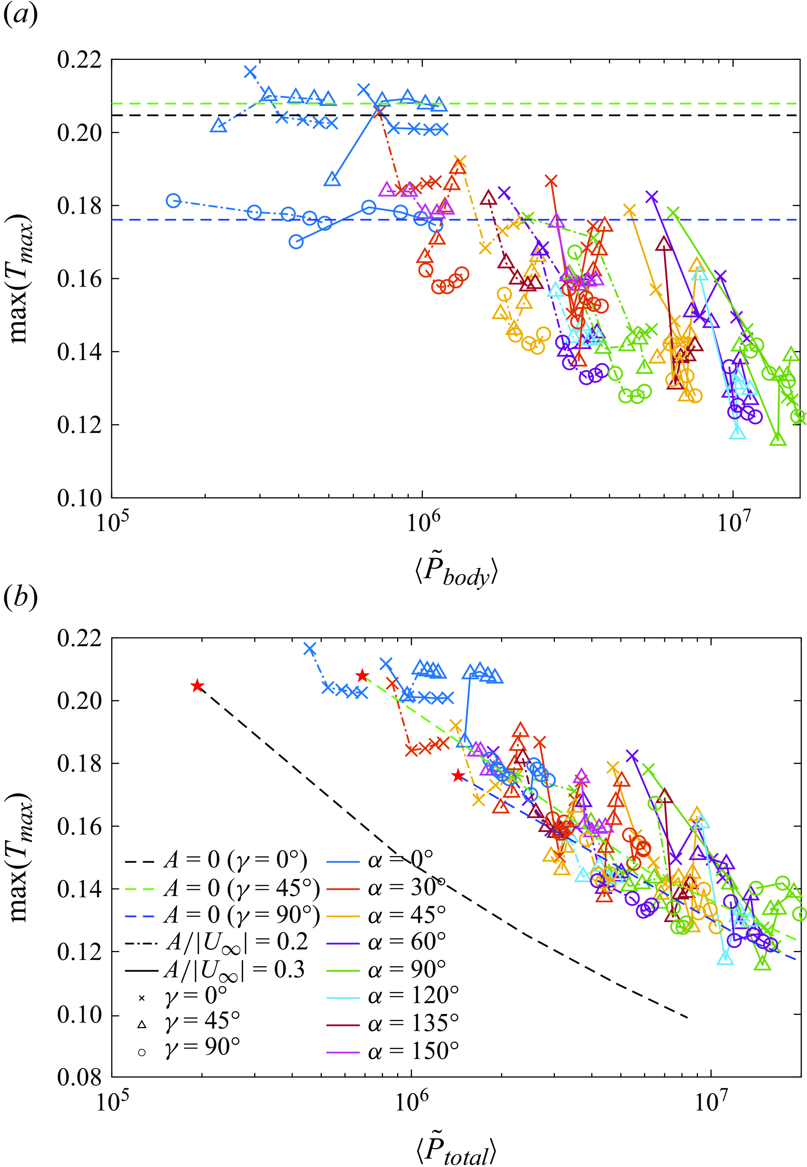
Figure 32. Value of $\max (T_{max })$
versus the time-averaged power needed to oscillate the plate (a), and the time-averaged total power including the power needed to drive the oncoming flow (b). The three horizontal dashed lines in (a) mark
$\max (T_{max })$
versus the time-averaged power needed to oscillate the plate (a), and the time-averaged total power including the power needed to drive the oncoming flow (b). The three horizontal dashed lines in (a) mark $\max (T_{max })$
for the steady plate. The three dashed curves in (b) show
$\max (T_{max })$
for the steady plate. The three dashed curves in (b) show $\max (T_{max })$
versus
$\max (T_{max })$
versus $\langle {\tilde {P}}_{total} \rangle$
for the steady plate. The values with
$\langle {\tilde {P}}_{total} \rangle$
for the steady plate. The values with $Re_U = 100$
are marked with red stars.
$Re_U = 100$
are marked with red stars.
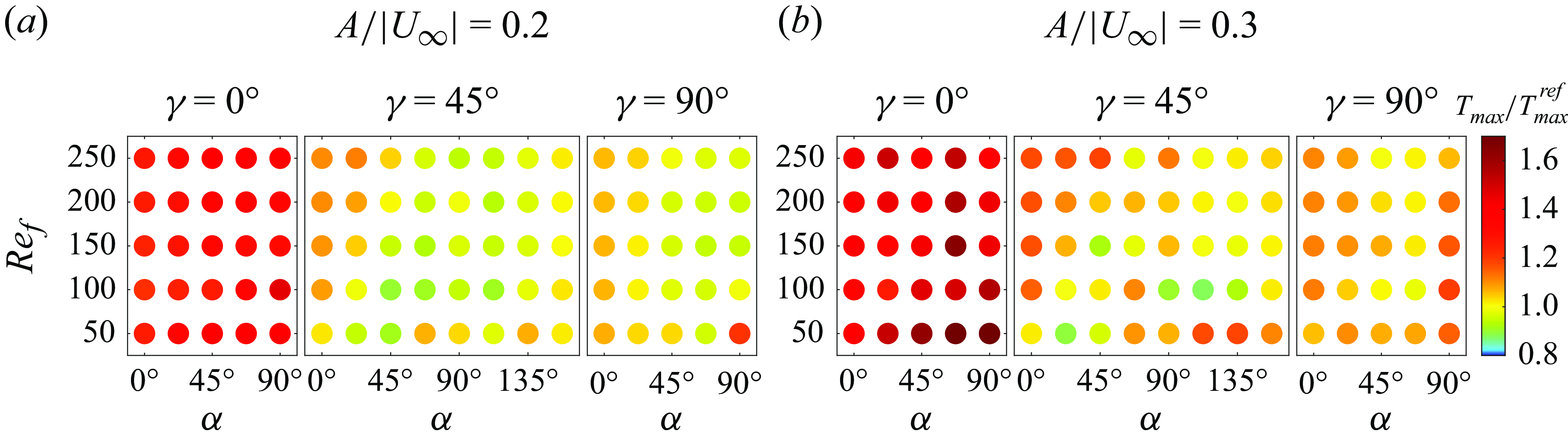
Figure 33. Comparison of $\max (T_{max })$
between the oscillating and stationary plate at the same total input power. Panels (a) and (b) correspond to
$\max (T_{max })$
between the oscillating and stationary plate at the same total input power. Panels (a) and (b) correspond to $A/|\boldsymbol{U}_{\infty }|=0.2$
and 0.3, respectively. The different colours of the filled circles in the
$A/|\boldsymbol{U}_{\infty }|=0.2$
and 0.3, respectively. The different colours of the filled circles in the $\alpha$
-
$\alpha$
- $Re_f$
plane correspond to different values of the ratio of
$Re_f$
plane correspond to different values of the ratio of $\max (T_{max })/ \max (T_{max })^{{ref}}$
, with
$\max (T_{max })/ \max (T_{max })^{{ref}}$
, with $\max (T_{max })$
and
$\max (T_{max })$
and $\max (T_{max })^{{ref}}$
computed for the oscillating and stationary plate at the same total input power evaluated with equation (5.5).
$\max (T_{max })^{{ref}}$
computed for the oscillating and stationary plate at the same total input power evaluated with equation (5.5).
If the oncoming flow is free, the conclusions from figure 30(a) are similar to those with fixed temperature, as $\langle T_{{avg}} \rangle$
is inversely related to
$\langle T_{{avg}} \rangle$
is inversely related to $\langle \overline {Nu} \rangle$
: the optimal cases have
$\langle \overline {Nu} \rangle$
: the optimal cases have $\gamma =45^\circ$
or
$\gamma =45^\circ$
or $\gamma =90^\circ$
. As
$\gamma =90^\circ$
. As $\langle T_{{avg}} \rangle$
decreases along the Pareto front, the optimal cases transition from
$\langle T_{{avg}} \rangle$
decreases along the Pareto front, the optimal cases transition from $A/|\boldsymbol{U}_{\infty }|=0.2$
to
$A/|\boldsymbol{U}_{\infty }|=0.2$
to $A/|\boldsymbol{U}_{\infty }|=0.3$
. These observations also apply for
$A/|\boldsymbol{U}_{\infty }|=0.3$
. These observations also apply for $\max (T_{max })$
versus
$\max (T_{max })$
versus $\langle \tilde {P}_{{body}} \rangle$
, as shown in figure 32(a). Here, many of the optimal cases correspond to
$\langle \tilde {P}_{{body}} \rangle$
, as shown in figure 32(a). Here, many of the optimal cases correspond to $\gamma =90^\circ$
. The reason might be that the transverse flow sets no preferences for vortex grouping at the two edges, which leads to a relatively even temperature distribution, lowering the temperature at the hottest spot.
$\gamma =90^\circ$
. The reason might be that the transverse flow sets no preferences for vortex grouping at the two edges, which leads to a relatively even temperature distribution, lowering the temperature at the hottest spot.
If the total power in (5.5) is considered, the Pareto frontier is again the steady plate with $\gamma =0^\circ$
, as shown in panels (b) of figures 30 and 32. Again, the oscillating plates at low
$\gamma =0^\circ$
, as shown in panels (b) of figures 30 and 32. Again, the oscillating plates at low $Re_f$
with
$Re_f$
with $\gamma =45^\circ$
or
$\gamma =45^\circ$
or $\gamma =90^\circ$
outperform the steady plates at
$\gamma =90^\circ$
outperform the steady plates at $\gamma =45^\circ$
or
$\gamma =45^\circ$
or $\gamma =90^\circ$
, but they still consume much more energy than the steady plate at
$\gamma =90^\circ$
, but they still consume much more energy than the steady plate at $\gamma =0^\circ$
for given
$\gamma =0^\circ$
for given $\langle T_{{avg}} \rangle$
or
$\langle T_{{avg}} \rangle$
or $\max (T_{max })$
.
$\max (T_{max })$
.
Similar to the fixed-temperature case, we define two performance measures, $\langle T_{{avg}} \rangle / \langle T_{{avg}} \rangle ^{{ref}}$
and
$\langle T_{{avg}} \rangle / \langle T_{{avg}} \rangle ^{{ref}}$
and $\max (T_{max })/ \max (T_{max })^{{ref}}$
, which compare
$\max (T_{max })/ \max (T_{max })^{{ref}}$
, which compare $\langle T_{{avg}} \rangle$
and
$\langle T_{{avg}} \rangle$
and $\max (T_{max })$
with the non-oscillating plate with the same orientation in the flow and at the same total input power. The oscillating plate is considered outperform the non-oscillating plate if
$\max (T_{max })$
with the non-oscillating plate with the same orientation in the flow and at the same total input power. The oscillating plate is considered outperform the non-oscillating plate if $\langle T_{{avg}} \rangle / \langle T_{{avg}} \rangle ^{{ref}}$
or
$\langle T_{{avg}} \rangle / \langle T_{{avg}} \rangle ^{{ref}}$
or $\max (T_{max })/ \max (T_{max })^{{ref}}$
is less than 1.
$\max (T_{max })/ \max (T_{max })^{{ref}}$
is less than 1.
The results of $\langle T_{{avg}} \rangle / \langle T_{{avg}} \rangle ^{{ref}}$
are shown in figure 31. Again, since
$\langle T_{{avg}} \rangle / \langle T_{{avg}} \rangle ^{{ref}}$
are shown in figure 31. Again, since $\langle T_{{avg}} \rangle$
is anti-correlated to
$\langle T_{{avg}} \rangle$
is anti-correlated to $\langle \overline {Nu} \rangle$
, we can draw similar conclusions as the fixed-temperature case. The stationary plate is always better than the oscillating plate at
$\langle \overline {Nu} \rangle$
, we can draw similar conclusions as the fixed-temperature case. The stationary plate is always better than the oscillating plate at $\gamma =0^\circ$
. As
$\gamma =0^\circ$
. As $\alpha$
gets closer to
$\alpha$
gets closer to $90^\circ$
, more cases have the oscillating plate outperforming the stationary plate at
$90^\circ$
, more cases have the oscillating plate outperforming the stationary plate at $\gamma =45^\circ$
and
$\gamma =45^\circ$
and $\gamma =90^\circ$
. With
$\gamma =90^\circ$
. With $\alpha$
fixed,
$\alpha$
fixed, $\langle T_{{avg}} \rangle / \langle T_{{avg}} \rangle ^{{ref}}$
increases with
$\langle T_{{avg}} \rangle / \langle T_{{avg}} \rangle ^{{ref}}$
increases with $Re_f$
at
$Re_f$
at $\gamma =45^\circ$
and
$\gamma =45^\circ$
and $\gamma =90^\circ$
, indicating that oscillations at lower
$\gamma =90^\circ$
, indicating that oscillations at lower $Re_f$
are more beneficial to heat transfer.
$Re_f$
are more beneficial to heat transfer.
The results of $\max (T_{max })/ \max (T_{max })^{{ref}}$
are shown in figure 33. The conclusions for
$\max (T_{max })/ \max (T_{max })^{{ref}}$
are shown in figure 33. The conclusions for $\max (T_{max })$
are generally similar to those for
$\max (T_{max })$
are generally similar to those for $\langle T_{{avg}} \rangle$
. However, for
$\langle T_{{avg}} \rangle$
. However, for $\gamma =45^\circ$
and
$\gamma =45^\circ$
and $90^\circ$
, many cases at the lowest
$90^\circ$
, many cases at the lowest $Re_f=50$
have the stationary plate outperforming the oscillating plate, which indicates that, although the oscillation at low
$Re_f=50$
have the stationary plate outperforming the oscillating plate, which indicates that, although the oscillation at low $Re_f$
helps lower the average temperature of the plate, it might also induce an uneven temperature distribution with a specific region very hot. Also, as
$Re_f$
helps lower the average temperature of the plate, it might also induce an uneven temperature distribution with a specific region very hot. Also, as $A/|\boldsymbol{U}_{\infty }|$
increased from 0.2 to 0.3, less cases have the oscillating plate better than the stationary plate, and the variation of
$A/|\boldsymbol{U}_{\infty }|$
increased from 0.2 to 0.3, less cases have the oscillating plate better than the stationary plate, and the variation of $\max (T_{max })/ \max (T_{max })^{{ref}}$
with
$\max (T_{max })/ \max (T_{max })^{{ref}}$
with $Re_f$
becomes more irregular. This might be related to the more irregular flows at
$Re_f$
becomes more irregular. This might be related to the more irregular flows at $A/|\boldsymbol{U}_{\infty }|=0.3$
. The value of
$A/|\boldsymbol{U}_{\infty }|=0.3$
. The value of $\max (T_{max })$
is sensitive to the flow and temperature details corresponding to a specific instant when the maximum temperature occurs, which make the variation of
$\max (T_{max })$
is sensitive to the flow and temperature details corresponding to a specific instant when the maximum temperature occurs, which make the variation of $\max (T_{max })/ \max (T_{max })^{{ref}}$
with the parameters less regular than the space and time-averaged quantities,
$\max (T_{max })/ \max (T_{max })^{{ref}}$
with the parameters less regular than the space and time-averaged quantities, $\langle \overline {Nu} \rangle$
and
$\langle \overline {Nu} \rangle$
and $\langle T_{{avg}} \rangle$
.
$\langle T_{{avg}} \rangle$
.


 Open access