


1. Introduction
Over the past few decades, there has been significant and growing interest in the field of microfluidics and in the development of lab-on-a-chip devices (see, for example, Beebe, Mensing & Walker Reference Beebe, Mensing and Walker2002; Stone, Stroock & Ajdari Reference Stone, Stroock and Ajdari2004; Squires & Quake Reference Squires and Quake2005; Dittrich & Manz Reference Dittrich and Manz2006; Sackmann, Fulton & Beebe Reference Sackmann, Fulton and Beebe2014; Nguyen, Wereley & Shaegh Reference Nguyen, Wereley and Shaegh2019; Battat, Weitz & Whitesides Reference Battat, Weitz and Whitesides2022). In particular, microfluidic devices are often used to generate and manipulate arrays of bubbles or droplets (see Anna Reference Anna2016; Zhu & Wang Reference Zhu and Wang2017) that are completely surrounded by an immiscible liquid. We study bubbles in Hele-Shaw geometries that are flattened by the channel walls and thus assume pancake-like shapes (Zhu & Gallaire Reference Zhu and Gallaire2016) with thin liquid films separating the bubble from the walls. We focus on bubbles that are small enough such that, due to the effects of surface tension, they remain approximately circular when viewed from above. This regime is relevant to many practical Hele-Shaw geometries (see, for example, Maxworthy Reference Maxworthy1986; Beatus, Tlusty & Bar-Ziv Reference Beatus, Tlusty and Bar-Ziv2006; Huerre, Miralles & Jullien Reference Huerre, Miralles and Jullien2014; Shen et al. Reference Shen, Leman, Reyssat and Tabeling2014; Gnyawali et al. Reference Gnyawali, Moon, Kieda, Karshafian, Kolios and Tsai2017).
A general model for the motion of such bubbles in a uniform background flow was developed by Booth, Griffiths & Howell (Reference Booth, Griffiths and Howell2023), who presented results for the motion of isolated bubbles and arrays of identical bubbles. This model was later generalised to the case of buoyancy-driven flow and extended to allow for bubble deformation (Wu et al. Reference Wu, Booth, Griffiths, Howell, Nunes and Stone2024). In the present paper, the model is applied to study the hydrodynamic interactions of a pair of bubbles of arbitrary radii. Understanding and characterising two-body problems is a common starting point in the study of suspensions (see, for example, Frankel & Andreas Reference Frankel and Andreas1967). In dilute suspensions, pairwise hydrodynamic interactions between particles are of principal importance, and they are used to construct first approximations of an effective viscosity (Batchelor & Green Reference Batchelor and Green1972; Batchelor Reference Batchelor1977). Moreover, studies of two particles have provided significant insight into the collision, aggregation and coalescence of particles (see, for example, Stoos, Yang & Leal Reference Stoos, Yang and Leal1992; Leal Reference Leal2004; Arp & Mason Reference Arp and Mason1977a ), processes that have a significant impact on the composition of suspensions over time. We analyse two phenomena involving pairs of bubbles that are relevant both for the propagation of bubble suspensions in narrow channels and for the control of bubble arrays in microfluidic channels.
The first phenomenon concerns a pair of circular bubbles of different radii. Since the larger bubble travels faster than the smaller one (Booth et al. Reference Booth, Griffiths and Howell2023; Wu et al. Reference Wu, Booth, Griffiths, Howell, Nunes and Stone2024), the distance between the bubbles decreases when the larger bubble is behind the smaller one. As the larger bubble approaches the smaller one, hydrodynamic interactions cause them to roll over each other and avoid contact under certain circumstances. This is similar to how lubrication forces prevent the contact of rigid spheres and cylinders approaching each other in shear flow (Bartok & Mason Reference Bartok and Mason1957; Darabaner, Raasch & Mason Reference Darabaner, Raasch and Mason1967; Arp & Mason Reference Arp and Mason1977b ). However, for the model that we examine, there are circumstances in which two bubbles will collide. Our analysis of the ‘rollover’ phenomenon includes an investigation of the conditions under which it may fail and the bubbles collide instead. The second phenomenon concerns two bubbles on the same streamline. When they are in close proximity, they deform so that the rear bubble becomes elongated and the front bubble becomes flattened. This shape change affects the bubble velocities, resulting in the eventual contact and coalescence of the bubbles. Analogous bubble phenomena, including deformation and coalescence of bubble pairs and smaller bubbles being ‘swept around’ larger ones, have been observed at low Reynolds numbers for buoyancy-driven bubbles in unconfined geometries in both experiments and numerical simulations (Manga & Stone Reference Manga and Stone1993). In Hele-Shaw geometries, deformation and pairing of single bubbles have been previously studied by Maxworthy (Reference Maxworthy1986). Shen et al. (Reference Shen, Leman, Reyssat and Tabeling2014) report observations and numerical simulations of pairs of droplets of different sizes reorienting themselves and aligning with the flow direction.
The interaction forces between circular bubbles or droplets in a Hele-Shaw cell are commonly approximated using a superposition of dipole solutions (see, for example, Beatus et al. Reference Beatus, Tlusty and Bar-Ziv2006), which is valid provided the bubbles are well separated. Sarig, Starosvetsky & Gat (Reference Sarig, Starosvetsky and Gat2016) obtained exact solutions for the interaction forces of two closely spaced circular droplets of arbitrary radii, relative position and velocities in a uniform background flow and additionally analysed the case in which the droplet velocities were determined by a force balance involving a free parameter describing the contribution of the droplets’ internal friction. Green (Reference Green2018) approximated the results of Sarig et al. (Reference Sarig, Starosvetsky and Gat2016) in order to develop a description of arbitrary numbers of identical circular droplets moving at the same velocity. In the present work, we examine the effect of the thin films above and below the bubble, resulting in a model with no free parameters. Using this model, we investigate the hydrodynamic interactions between pairs of circular bubbles of arbitrary radii. Particular attention is paid to the rollover phenomenon, which emerges as a result of these interactions under certain conditions.
We also investigate the deformation of a pair of bubbles that are aligned with the flow direction due to their hydrodynamic interactions. Generally, two identical circular bubbles or droplets in a Hele-Shaw cell aligned in the direction of the background flow are expected to travel together at some doublet velocity, which approaches that of an isolated bubble as the separation between the bubbles grows large (Sarig et al. Reference Sarig, Starosvetsky and Gat2016; Green Reference Green2018; Booth et al. Reference Booth, Griffiths and Howell2023). Analogous behaviour is seen for pairs of solid spheres (Happel & Brenner Reference Happel and Brenner2012). However, when deformable droplets or bubbles are in close proximity, they each experience distortions induced by the other (Manga & Stone Reference Manga and Stone1993Reference Manga and Stone1995). Such deformations break fore–aft symmetry and the reversibility of Stokes flow, leading to qualitatively different dynamics, some of which will be explored in our work. Irreversible particle interactions such as those we report would have significant implications on the microstructure and rheology of a suspension (Leighton & Acrivos Reference Leighton and Acrivos1987; Davis Reference Davis1993; Wilson & Davis Reference Wilson and Davis2000), as well as on the structure of bubble arrays propagating in microchannels.
The structure of this paper is as follows. In § 2, we summarise the general model developed by Booth et al. (Reference Booth, Griffiths and Howell2023) for the motion of a system of approximately circular pancake bubbles in a Hele-Shaw cell. In § 3, solutions are presented for the motion of a pair of circular bubbles of arbitrary radii. Experimental methods are described in § 4, and we present experimental and theoretical results for the motion of a pair of circular bubbles in § 5. In § 6, we focus on a pair of bubbles aligned in the flow direction and present theoretical and experimental results on the deformation of each bubble induced by the other. Finally, in § 7, we summarise our findings and discuss potential extensions of our work.
2. Mathematical modelling
2.1. Governing equations
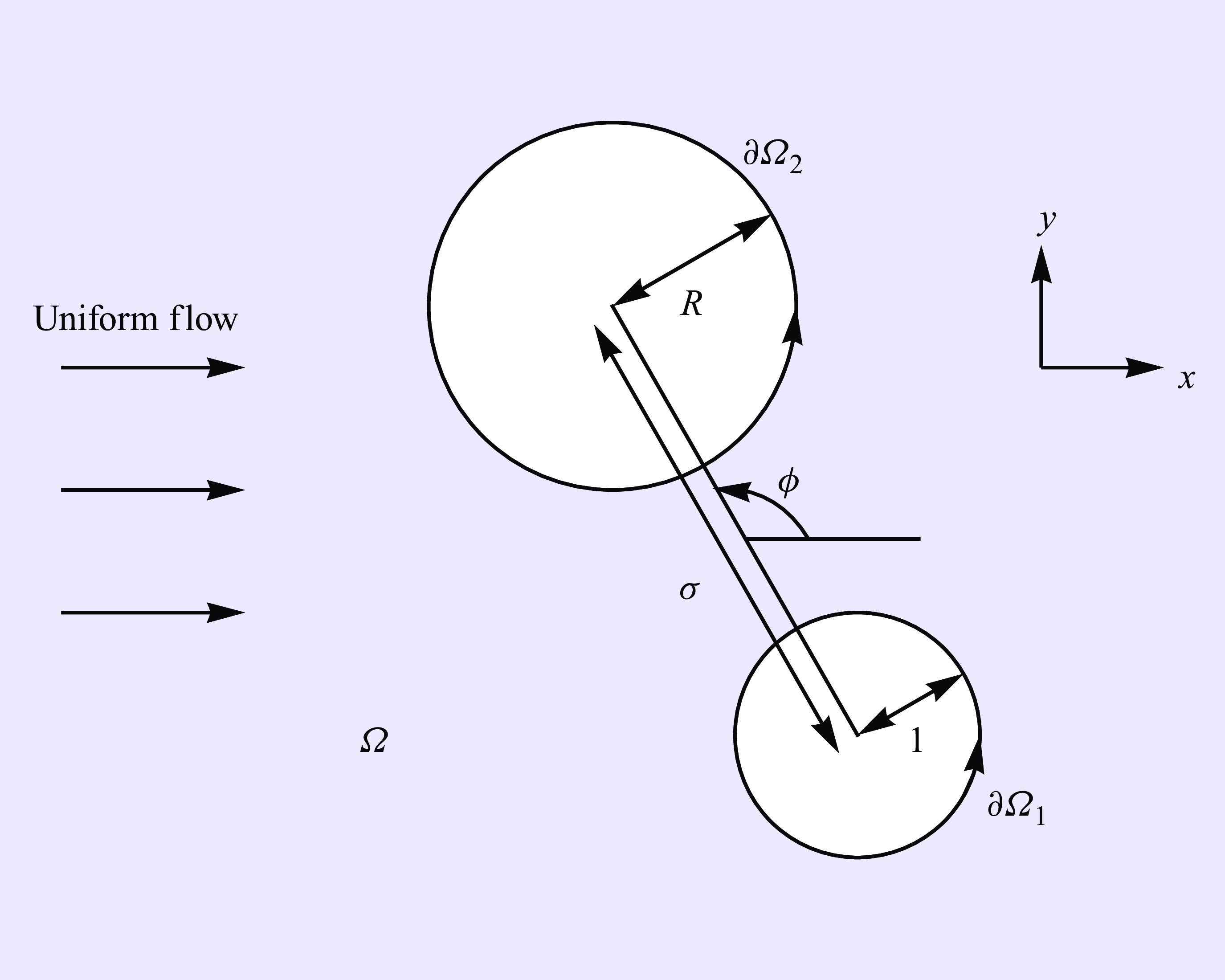
Figure 1. Schematic of the dimensionless two-bubble problem. The fluid domain is denoted by $\Omega$
and the the bubble surfaces are
$\Omega$
and the the bubble surfaces are $\partial \Omega _{1,2}$
. We supply a uniform outer flow far from the bubbles. The bubble centre–centre distance is
$\partial \Omega _{1,2}$
. We supply a uniform outer flow far from the bubbles. The bubble centre–centre distance is $\sigma$
and the angle the bubbles make to the direction of the outer flow is
$\sigma$
and the angle the bubbles make to the direction of the outer flow is $\phi$
.
$\phi$
.
As in Booth et al. (Reference Booth, Griffiths and Howell2023), we consider the motion of two bubbles in a Hele-Shaw cell of height $\hat {h}$
parallel to the
$\hat {h}$
parallel to the $(\hat {x}, \hat {y})$
-plane. Here,
$(\hat {x}, \hat {y})$
-plane. Here, $\hat {h}$
is assumed to be much smaller than the horizontal dimensions of the cell and the bubbles, so we can employ lubrication theory. The bubbles are flattened by the cell walls above and below into pancake-like shapes with approximately circular profiles when viewed from above (figure 1), whose radii are denoted by
$\hat {h}$
is assumed to be much smaller than the horizontal dimensions of the cell and the bubbles, so we can employ lubrication theory. The bubbles are flattened by the cell walls above and below into pancake-like shapes with approximately circular profiles when viewed from above (figure 1), whose radii are denoted by $\hat {R}_1$
and
$\hat {R}_1$
and $\hat {R}_2$
, where
$\hat {R}_2$
, where $\hat {R}_{1,2}\gg \hat {h}$
. We prescribe a uniform unidirectional flow with velocity
$\hat {R}_{1,2}\gg \hat {h}$
. We prescribe a uniform unidirectional flow with velocity $\hat {U}\boldsymbol {i}$
in the far field (where
$\hat {U}\boldsymbol {i}$
in the far field (where $\boldsymbol {i}$
denotes the unit vector in the
$\boldsymbol {i}$
denotes the unit vector in the $\hat {x}$
-direction). The viscosity of the liquid and the liquid–air surface tension are denoted by
$\hat {x}$
-direction). The viscosity of the liquid and the liquid–air surface tension are denoted by $\hat {\mu }$
and
$\hat {\mu }$
and $\hat {\gamma }$
, respectively.
$\hat {\gamma }$
, respectively.
We non-dimensionalise the system by scaling lengths with $\hat {R}_1$
, velocities with
$\hat {R}_1$
, velocities with $\hat {U}$
, the fluid pressure
$\hat {U}$
, the fluid pressure $\hat {p}$
with
$\hat {p}$
with $12\hat {\mu }\hat {U}\hat {R}_1/{\hat {h}}^2$
and the pressure inside the
$12\hat {\mu }\hat {U}\hat {R}_1/{\hat {h}}^2$
and the pressure inside the $k$
th bubble,
$k$
th bubble, $\hat {p}_k$
, with
$\hat {p}_k$
, with $2\hat {\gamma } / \hat {h}$
, where
$2\hat {\gamma } / \hat {h}$
, where $\hat {\gamma }$
is the surface tension. This procedure gives the following dimensionless model, in which dimensionless variables are denoted without hats:
$\hat {\gamma }$
is the surface tension. This procedure gives the following dimensionless model, in which dimensionless variables are denoted without hats:
 \begin{align} \nabla ^2 p & = 0 \qquad\qquad\qquad\qquad\qquad\qquad\qquad\qquad\quad\text {in} \quad \Omega , \end{align}
 \begin{align} \boldsymbol {n}\boldsymbol {\cdot } \boldsymbol {\nabla } p & = -U_{n,k} \qquad\qquad\qquad\qquad\qquad\qquad\qquad\quad\!\text{on} \quad\!\partial \Omega _{k}, \end{align}
 \begin{align} p_k - \frac {3\mathrm {Ca}}{\epsilon } p & = 1 + \mathrm {Ca}^{2/3}\beta \left (U_{n,k}\right ) \left (U_{n,k}\right )^{2/3} + \frac {\epsilon \pi }{4}\kappa _k \quad\quad\,\,\,\mbox {on} \quad\!\partial \Omega _k, \end{align}
 \begin{align} \boldsymbol {\nabla }p&\rightarrow -\boldsymbol {i} \qquad\qquad\qquad\qquad\qquad\qquad\qquad\qquad \text {as} \quad x^2 +y^2 \rightarrow \infty . \end{align}
Here, $\Omega$
is the fluid domain, while
$\Omega$
is the fluid domain, while $\partial \Omega _k$
,
$\partial \Omega _k$
, $\kappa _k$
and
$\kappa _k$
and $U_{n,k}$
are the boundary, in-plane curvature and local normal velocity of the interface of the
$U_{n,k}$
are the boundary, in-plane curvature and local normal velocity of the interface of the $k$
th bubble, respectively (
$k$
th bubble, respectively ( $k=1,2$
), and
$k=1,2$
), and $\beta$
is the Bretherton coefficient, whose value depends on whether the meniscus is advancing or retreating (Bretherton Reference Bretherton1961; Wong, Radke & Morris Reference Wong, Radke and Morris1995; Halpern & Jensen Reference Halpern and Jensen2002)
$\beta$
is the Bretherton coefficient, whose value depends on whether the meniscus is advancing or retreating (Bretherton Reference Bretherton1961; Wong, Radke & Morris Reference Wong, Radke and Morris1995; Halpern & Jensen Reference Halpern and Jensen2002)
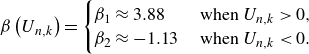 \begin{equation} \beta \left (U_{n,k}\right )=\begin{cases} \beta _1 \approx 3.88 & \text { when }U_{n,k} \gt 0,\\ \beta _2 \approx -1.13 & \text { when }U_{n,k} \lt 0. \end{cases} \end{equation}
The boundary condition (2.1c) was proposed by Meiburg (Reference Meiburg1989) and later derived by Burgess & Foster (Reference Burgess and Foster1990). In (2.1b ) we neglect to include the contribution due to leakage into the thin films because this effect is always subdominant. However, this effect could easily be included in the model (see, for example Burgess & Foster Reference Burgess and Foster1990; Peng et al. Reference Peng, Pihler-Puzović, Juel, Heil and Lister2015; Wu et al. Reference Wu, Booth, Griffiths, Howell, Nunes and Stone2024).
The system (2.1) contains two dimensionless parameters: the bubble aspect ratio and the capillary number, defined by
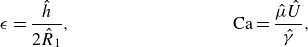 \begin{align} \epsilon & = \frac {\hat {h}}{2\hat {R}_1}, & \mathrm {Ca} &= \frac {\hat {\mu } \hat {U}}{\hat {\gamma }}, \end{align}
respectively, both of which are assumed to be small. Specifically, in the distinguished limit $\mathrm {Ca}=O(\epsilon ^3)$
, the viscous pressure balances the pressure drop across the menisci (the second and fourth terms in (2.1c
)). In this regime, both bubbles remain circular to leading order, so
$\mathrm {Ca}=O(\epsilon ^3)$
, the viscous pressure balances the pressure drop across the menisci (the second and fourth terms in (2.1c
)). In this regime, both bubbles remain circular to leading order, so $U_{n,k}=\boldsymbol {U}_k\boldsymbol {\cdot }\boldsymbol {n}$
and
$U_{n,k}=\boldsymbol {U}_k\boldsymbol {\cdot }\boldsymbol {n}$
and $p$
is therefore fully determined by the problem (2.1a
), (2.1b
) and (2.1d
) (up to an irrelevant constant) once the bubble velocities
$p$
is therefore fully determined by the problem (2.1a
), (2.1b
) and (2.1d
) (up to an irrelevant constant) once the bubble velocities $\boldsymbol {U}_k$
are specified. As a shortcut to determine the bubble velocities we perform an effective net force balance by integrating (2.1c
) around each bubble (see, for example, Booth et al. Reference Booth, Griffiths and Howell2023), to obtain
$\boldsymbol {U}_k$
are specified. As a shortcut to determine the bubble velocities we perform an effective net force balance by integrating (2.1c
) around each bubble (see, for example, Booth et al. Reference Booth, Griffiths and Howell2023), to obtain
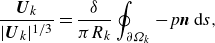 \begin{equation} \frac {\boldsymbol {U}_k}{|\boldsymbol {U}_k|^{1/3}} =\frac {\delta }{\pi R_k}\oint _{\partial \Omega _k} -p\boldsymbol {n}\, \mathrm {d}s, \end{equation}
where $R_k$
is the dimensionless radius of the
$R_k$
is the dimensionless radius of the $k$
th bubble. The resulting problem contains a single dimensionless group, the Bretherton parameter, defined by
$k$
th bubble. The resulting problem contains a single dimensionless group, the Bretherton parameter, defined by
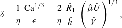 \begin{equation} \delta = \frac {1}{\eta }\, \frac {\mathrm {Ca}^{1/3}}{\epsilon } = \frac {2}{\eta }\,\frac {\hat {R}_1}{\hat {h}}\,\left (\frac {\hat {\mu }\hat {U}}{\hat {\gamma }}\right )^{1/3}, \end{equation}
which is assumed to be $O(1)$
while
$O(1)$
while $\epsilon$
and
$\epsilon$
and $\mathrm {Ca}$
both tend to zero. The numerical constant
$\mathrm {Ca}$
both tend to zero. The numerical constant
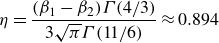 \begin{equation} \eta =\frac {(\beta _1-\beta _2)\Gamma (4/3)}{3\sqrt {\pi }\Gamma (11/6)}\approx 0.894 \end{equation}
incorporates the Bretherton pressure drops (2.2) across the advancing and retreating menisci (Bretherton Reference Bretherton1961; Wu et al. Reference Wu, Booth, Griffiths, Howell, Nunes and Stone2024).
The Bretherton parameter is a dimensionless parameter that compares the magnitudes of the viscous pressure from the flow around the bubble and of the Bretherton pressure, or the pressure drop across the thin films surrounding the bubble. As $\delta$
increases to infinity, the viscous pressure dominates over the Bretherton pressure. In this limit, we recover the result due to Taylor & Saffman (Reference Taylor and Saffman1959) that the bubble moves at twice the background flow velocity, which was obtained while disregarding the thin film drag. Booth et al. (Reference Booth, Griffiths and Howell2023) showed that an isolated circular bubble travels parallel to the background flow with velocity
$\delta$
increases to infinity, the viscous pressure dominates over the Bretherton pressure. In this limit, we recover the result due to Taylor & Saffman (Reference Taylor and Saffman1959) that the bubble moves at twice the background flow velocity, which was obtained while disregarding the thin film drag. Booth et al. (Reference Booth, Griffiths and Howell2023) showed that an isolated circular bubble travels parallel to the background flow with velocity $\boldsymbol {U}_b=U_b\boldsymbol {i}$
, where
$\boldsymbol {U}_b=U_b\boldsymbol {i}$
, where $U_b$
is a monotonically increasing function of
$U_b$
is a monotonically increasing function of $\delta$
, satisfying
$\delta$
, satisfying $U_b\rightarrow 0$
as
$U_b\rightarrow 0$
as $\delta \rightarrow 0$
and
$\delta \rightarrow 0$
and $U_b\rightarrow 2$
as
$U_b\rightarrow 2$
as $\delta \rightarrow \infty$
. Importantly for this work, it follows that larger bubbles travel faster than smaller ones when all other parameters are fixed, since
$\delta \rightarrow \infty$
. Importantly for this work, it follows that larger bubbles travel faster than smaller ones when all other parameters are fixed, since $\delta \propto \hat {R}_1$
. This conclusion may also be drawn using dimensional analysis, through which it can be shown that the driving force due to the background flow is proportional to
$\delta \propto \hat {R}_1$
. This conclusion may also be drawn using dimensional analysis, through which it can be shown that the driving force due to the background flow is proportional to $\hat {R}_1^2$
and the drag force due to the thin films is proportional to
$\hat {R}_1^2$
and the drag force due to the thin films is proportional to $\hat {R}_1$
.
$\hat {R}_1$
.
2.2. Complex variable formulation
We now reformulate the problem (2.1) in terms of complex variables. At leading order we have two circular bubbles whose centroids are at positions $(x_1,y_1)$
and
$(x_1,y_1)$
and $(x_2,y_2)$
in the
$(x_2,y_2)$
in the $(x,y)$
-plane, with a uniform velocity in the far field of unit magnitude. We label the bubbles such that the smaller bubble is located at
$(x,y)$
-plane, with a uniform velocity in the far field of unit magnitude. We label the bubbles such that the smaller bubble is located at $(x_1,y_1)$
and the dimensionless radii of the two bubbles are thus
$(x_1,y_1)$
and the dimensionless radii of the two bubbles are thus $R_1=1$
and
$R_1=1$
and $R_2 =R$
, where
$R_2 =R$
, where $R\geqslant 1$
is the radius ratio of the two bubbles. As shown schematically in figure 1, the problem is instantaneously characterised by the length
$R\geqslant 1$
is the radius ratio of the two bubbles. As shown schematically in figure 1, the problem is instantaneously characterised by the length $\sigma$
of the vector joining the smaller bubble centre to the larger bubble centre, the angle
$\sigma$
of the vector joining the smaller bubble centre to the larger bubble centre, the angle $\phi$
that it makes with the
$\phi$
that it makes with the $x$
-axis (which is parallel to the background flow direction), and the radius ratio
$x$
-axis (which is parallel to the background flow direction), and the radius ratio $R$
.
$R$
.
Since the flow is governed by Laplace’s equation, we can formulate this as a problem for the complex potential $w(z)=-p+\mathrm {i}\psi$
, where
$w(z)=-p+\mathrm {i}\psi$
, where $\psi$
is the streamfunction, and
$\psi$
is the streamfunction, and $z=x+\mathrm {i}y$
. Then
$z=x+\mathrm {i}y$
. Then $w(z)$
is holomorphic in the region
$w(z)$
is holomorphic in the region $\Omega$
outside the two bubbles and satisfies the boundary conditions
$\Omega$
outside the two bubbles and satisfies the boundary conditions
 \begin{align} \quad\operatorname {Im}[w(z)] & = Q_1 + \operatorname {Im}\left (\overline {\mathcal {U}}_1 z\right ) \qquad\text {on} \quad |z-z_1| = R_1=1, \end{align}
 \begin{align} \operatorname {Im}[w(z)]& = Q_2 + \operatorname {Im}\left (\overline {\mathcal {U}}_2 z\right ) \qquad \text {on} \quad |z-z_2| = R_2=R\geqslant 1, \end{align}
 \begin{align} & w(z)\sim z +o(1) \qquad\quad \text {as} \quad z\rightarrow \infty , \end{align}
where, for $k \in \{1,2\}$
, we denote by
$k \in \{1,2\}$
, we denote by $z_k = x_k +\mathrm {i}y_k$
and
$z_k = x_k +\mathrm {i}y_k$
and $\mathcal {U}_k = U_k +\mathrm {i}V_k$
the complex representations of the
$\mathcal {U}_k = U_k +\mathrm {i}V_k$
the complex representations of the $k$
th bubble position and velocity, respectively, and the
$k$
th bubble position and velocity, respectively, and the $Q_k$
are a priori unknown constants. The over-bars denote complex conjugation. Note that (2.7a
) and (2.7c
) are the complex representations of the kinematic boundary conditions (see, for example, Crowdy Reference Crowdy2008).
$Q_k$
are a priori unknown constants. The over-bars denote complex conjugation. Note that (2.7a
) and (2.7c
) are the complex representations of the kinematic boundary conditions (see, for example, Crowdy Reference Crowdy2008).
Once we have solved for $w(z)$
, to close the system we evaluate the effective force balance (2.4) on each bubble, which in complex variables becomes
$w(z)$
, to close the system we evaluate the effective force balance (2.4) on each bubble, which in complex variables becomes
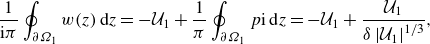 \begin{align} &\quad \frac {1}{\mathrm {i}\pi }\oint _{\partial \Omega _1} w(z)\,\mathrm {d}z=-\mathcal {U}_1+\frac {1}{\pi }\oint _{\partial \Omega _1}p\mathrm {i}\,\mathrm {d}z =-\mathcal {U}_1+\frac { \mathcal {U}_1}{\delta \left |\mathcal {U}_1\right |^{1/3}}, \end{align}
 \begin{align} &\frac {1}{\mathrm {i}\pi }\oint _{\partial \Omega _2} w(z)\,\mathrm {d}z=-R^2\mathcal {U}_2+\frac {1}{\pi }\oint _{\partial \Omega _2}p\mathrm {i}\,\mathrm {d}z =-R^2\mathcal {U}_2+\frac {R \mathcal {U}_2}{\delta \left |\mathcal {U}_2\right |^{1/3}}. \end{align}
Here $\partial \Omega _k$
is the boundary of the
$\partial \Omega _k$
is the boundary of the $k$
th bubble, given by
$k$
th bubble, given by $|z-z_k|=R_k$
.
$|z-z_k|=R_k$
.
The problem for the pressure field generated by two bubbles of unequal radii was solved by Sarig et al. (Reference Sarig, Starosvetsky and Gat2016) using a bipolar coordinate transformation, resulting in infinite series solutions for the interaction forces between the bubbles. Instead, using our complex variable formulation facilitates the evaluation of the integrals (2.8) in the force balance in closed form.
3. Solution for two bubbles of arbitrary radii
To begin we define the conformal map
 \begin{align} z=z_1+\mathrm {e}^{\mathrm {i}\phi }\left (\frac {1+a\zeta }{\zeta +a}\right ), \end{align}
from the the concentric annulus $A = \{\zeta : X\leqslant |\zeta |\leqslant 1\}$
onto the solution domain
$A = \{\zeta : X\leqslant |\zeta |\leqslant 1\}$
onto the solution domain $\Omega$
(see figure 2 for a schematic overview of the conformal mapping procedure), where
$\Omega$
(see figure 2 for a schematic overview of the conformal mapping procedure), where
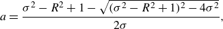 \begin{align} a & = \frac {\sigma ^2 -R^2 +1 - \sqrt {(\sigma ^2 -R^2 +1)^2-4\sigma ^2}}{2\sigma }, \end{align}
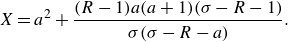 \begin{align} \quad X & = a^2+\frac {(R-1)a(a+1)(\sigma -R-1)}{\sigma (\sigma -R-\textit{a})}. \end{align}
Note that $a^2\leqslant X\lt a\lt 1$
. The conformal map is derived by first translating the fluid domain such that one of the bubbles is centred at the origin, then rotating so both bubble centres lie on the real axis, and finally applying a Möbius transformation to map the domain to a concentric annulus. In the mapping, the point at infinity in the
$a^2\leqslant X\lt a\lt 1$
. The conformal map is derived by first translating the fluid domain such that one of the bubbles is centred at the origin, then rotating so both bubble centres lie on the real axis, and finally applying a Möbius transformation to map the domain to a concentric annulus. In the mapping, the point at infinity in the $z$
-plane maps to
$z$
-plane maps to $-a$
in the
$-a$
in the $\zeta$
-plane, and
$\zeta$
-plane, and $X$
is the inner radius of the annulus.
$X$
is the inner radius of the annulus.
We then define $w(z) = z + W (\zeta )$
, where
$w(z) = z + W (\zeta )$
, where $W(\zeta )$
is holomorphic on the annulus,
$W(\zeta )$
is holomorphic on the annulus, $A$
, and satisfies the conditions
$A$
, and satisfies the conditions
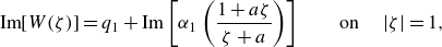 \begin{align} \operatorname {Im}[W(\zeta )] &= q_1 + \operatorname {Im}\left [\alpha _1 \left (\frac {1+a\zeta }{\zeta +a}\right )\right ]\qquad\text {on } \quad |\zeta | =1, \end{align}
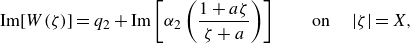 \begin{align} \operatorname {Im}[W(\zeta )] &= q_2 + \operatorname {Im}\left [\alpha _2 \left (\frac {1+a\zeta }{\zeta +a}\right )\right ] \qquad\text {on } \quad |\zeta | =X, \end{align}
with $\alpha _k = (\overline {\mathcal {U}}_k - 1)\mathrm {e}^{\mathrm {i}\phi }$
, and
$\alpha _k = (\overline {\mathcal {U}}_k - 1)\mathrm {e}^{\mathrm {i}\phi }$
, and $q_k = Q_k - \operatorname {Im}[(\overline {\mathcal {U}}_k - 1)z_1]$
.
$q_k = Q_k - \operatorname {Im}[(\overline {\mathcal {U}}_k - 1)z_1]$
.
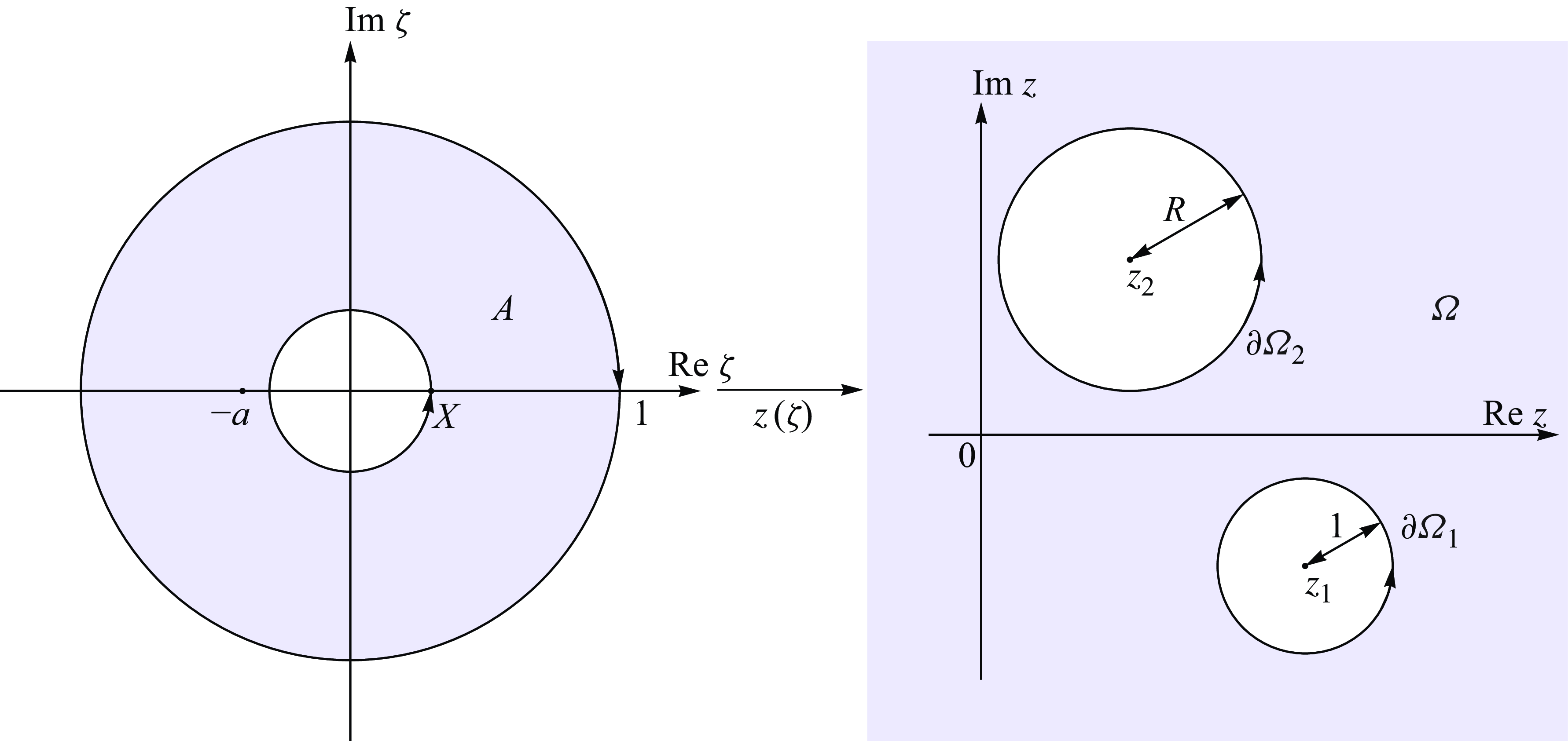
Figure 2. Schematic of the conformal map (3.1) from the annulus $A=\{\zeta : X\leqslant |\zeta |\leqslant 1\}$
in the
$A=\{\zeta : X\leqslant |\zeta |\leqslant 1\}$
in the $\zeta$
-plane to the fluid region
$\zeta$
-plane to the fluid region $\Omega$
in the
$\Omega$
in the $z$
-plane.
$z$
-plane.
Now we express $W(\zeta )$
as a Laurent expansion on
$W(\zeta )$
as a Laurent expansion on $A$
, i.e.
$A$
, i.e.
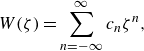 \begin{align} W(\zeta ) = \sum _{n=-\infty }^{\infty } c_n \zeta ^n, \end{align}
and use the boundary conditions (3.3) to calculate the coefficients $c_n$
. On
$c_n$
. On $|\zeta |=1$
we have
$|\zeta |=1$
we have $\overline {\zeta } = 1/\zeta$
so we can rearrange boundary condition (3.3a
) to
$\overline {\zeta } = 1/\zeta$
so we can rearrange boundary condition (3.3a
) to
 \begin{align} \operatorname {Im}[W(\zeta )] &= \operatorname {Im}[c_0] + \operatorname {Im}\left [\sum _{n=1}^{\infty } (c_n-\overline {c}_{-n})\zeta ^n\right ] \nonumber \\ &= q_1 - \operatorname {Im}[\overline {\alpha }_1 a] - \operatorname {Im}\left [\overline {\alpha }_1 \sum _{n=1}^{\infty } (1-a^2)(-a)^{n-1}\zeta ^n \right ]&&\text {on}\quad |\zeta |=1. \end{align}
It follows from (3.5) that
 \begin{align} c_n - \overline {c}_{-n} = \frac {\overline {\alpha }_1 (1-a^2)(-a)^n}{a} \qquad (n\geqslant 1), \end{align}
and, without loss of generality, we can choose $q_1 = \operatorname {Im}[\overline {\alpha }_1]a$
, so
$q_1 = \operatorname {Im}[\overline {\alpha }_1]a$
, so $c_0 = 0$
.
$c_0 = 0$
.
We progress similarly on $|\zeta | =X$
, where now
$|\zeta | =X$
, where now $\overline {\zeta } = X^2/\zeta$
. The boundary condition (3.3b
) can be rewritten as
$\overline {\zeta } = X^2/\zeta$
. The boundary condition (3.3b
) can be rewritten as
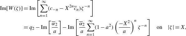 \begin{align} \operatorname {Im}[W(\zeta )] &=\operatorname {Im}\left [\sum _{n=1}^{\infty }(c_{-n}-X^{2n}\overline {c}_n)\zeta ^{-n}\right ] \nonumber \\ &= q_2 - \operatorname {Im}\left [\frac {\overline {\alpha }_2}{a}\right ] - \operatorname {Im}\left [\frac {\overline {\alpha }_2}{a}\sum _{n=1}^{\infty } (1-a^2)\left (\frac {-X^2}{a}\right )^n \zeta ^{-n}\right ] &&\text {on}\quad |\zeta |=X, \end{align}
and it follows that
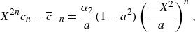 \begin{align} X^{2n}c_n - \overline {c}_{-n} = \frac {\alpha _2}{a}(1-a^2)\left (\frac {-X^2}{a}\right )^n, \end{align}
and $q_2 = \operatorname {Im}(\overline {\alpha }_2 /a)$
. We simultaneously solve equations (3.6) and (3.8) to find that the complex potential
$q_2 = \operatorname {Im}(\overline {\alpha }_2 /a)$
. We simultaneously solve equations (3.6) and (3.8) to find that the complex potential $W(\zeta )$
is given by
$W(\zeta )$
is given by
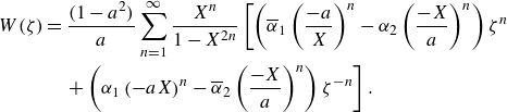 \begin{align} W(\zeta ) &= \frac {(1-a^2)}{a}\sum _{n=1}^{\infty } \frac {X^n}{1-X^{2n}}\left [\left (\overline {\alpha }_1 \left (\frac {-a}{X}\right )^n - \alpha _2\left (\frac {-X}{a}\right )^n \right )\zeta ^n \right.\notag\\ &\quad\left. + \left (\alpha _1 \left (-aX\right )^n - \overline {\alpha }_2\left (\frac {-X}{a}\right )^n \right )\zeta ^{-n}\right ]. \end{align}
The equations of motion for the bubbles can be found from (2.8) via
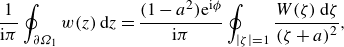 \begin{align} \frac {1}{\mathrm {i}\pi } \oint _{\partial \Omega _1} w(z) \, \mathrm {d}z &= \frac {(1-a^2) \mathrm {e}^{\mathrm {i}\phi }}{\mathrm {i}\pi } \oint _{|\zeta |=1} \frac {W(\zeta )\, \mathrm {d}\zeta }{(\zeta + a)^2} , \end{align}
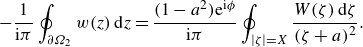 \begin{align} -\frac {1}{\mathrm {i}\pi } \oint _{\partial \Omega _2} w(z) \, \mathrm {d}z &= \frac {(1-a^2) \mathrm {e}^{\mathrm {i}\phi }}{\mathrm {i}\pi } \oint _{|\zeta |=X} \frac {W(\zeta )\, \mathrm {d}\zeta }{(\zeta + a)^2} . \end{align}
The integrand in (3.10a
) has poles at $\zeta = -a$
and
$\zeta = -a$
and $0$
, whereas (3.10b
) only has a pole at
$0$
, whereas (3.10b
) only has a pole at $\zeta = 0$
. The residue due to the pole at
$\zeta = 0$
. The residue due to the pole at $\zeta = 0$
is the same for both integrals and can be calculated to give
$\zeta = 0$
is the same for both integrals and can be calculated to give
 \begin{align} \operatorname {Res}\left [\frac {W(\zeta )}{(\zeta + a)^2};\zeta =0\right ] = \frac {1-a^2}{a^2}\sum _{n=1}^{\infty } \frac {nX^{2n}}{1-X^{2n}}\left [\frac {(\mathcal {U}_2 -1)\mathrm {e}^{-\mathrm {i}\phi }}{a^{2n}}-(\overline {\mathcal {U}}_1 -1)\mathrm {e}^{\mathrm {i}\phi } \right ]. \end{align}
The residue at $\zeta = -a$
is given by
$\zeta = -a$
is given by
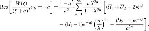 \begin{align} \operatorname {Res}\left [\frac {W(\zeta )}{(\zeta + a)^2};\zeta =-a\right ] &= \frac {1-a^2}{a^2}\sum _{n=1}^{\infty } \frac {nX^{2n}}{1-X^{2n}}\left [(\overline {\mathcal {U}}_1 + \overline {\mathcal {U}}_2 -2)\mathrm {e}^{\mathrm {i}\phi } \phantom {\left (\frac {a}{X}\right )^{2n}}\right . \nonumber \\ &\quad - \left.(\mathcal {U}_1 -1)\mathrm {e}^{-\mathrm {i}\phi } \left (\frac {a}{X}\right )^{2n} - \frac {(\mathcal {U}_2 -1)\mathrm {e}^{-\mathrm {i}\phi }}{a^{2n}} \right ]. \end{align}
Thus, by Cauchy’s residue theorem, we find
 \begin{align} \frac {1}{\mathrm {i}\pi } \oint _{\partial \Omega _1} w(z) \, \mathrm {d}z &= f_1(\sigma ,R) \bigl (\overline {\mathcal {U}}_2 -1\bigr )\mathrm {e}^{2\mathrm {i}\phi } -f_2(\sigma ,R) \bigl (\mathcal {U}_1 -1\bigr ) , \end{align}
 \begin{align} \frac {1}{\mathrm {i}\pi } \oint _{\partial \Omega _2} w(z) \, \mathrm {d}z &= f_1(\sigma ,R) \bigl (\overline {\mathcal {U}}_1-1\bigr )\mathrm {e}^{2\mathrm {i}\phi }- f_3(\sigma ,R) \bigl (\mathcal {U}_2 -1\bigr ), \end{align}
where
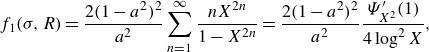 \begin{align} &\qquad\qquad f_1(\sigma ,R) = \frac {2(1-a^2)^2}{a^2}\sum _{n=1}^{\infty } \frac {nX^{2n}}{1-X^{2n}}=\frac {2(1-a^2)^2}{a^2} \frac {\Psi _{X^2}^{\prime}(1)}{4 \log ^2X}, \end{align}
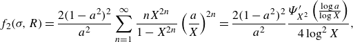 \begin{align} &\quad f_2(\sigma ,R) = \frac {2(1-a^2)^2}{a^2}\sum _{n=1}^{\infty } \frac {nX^{2n}}{1-X^{2n}} \left (\frac {a}{X}\right )^{2n} = \frac {2(1-a^2)^2}{a^2} \frac {\Psi^{\prime} _{X^2}\left (\frac {\log a}{\log X}\right )}{4 \log ^2X}, \end{align}
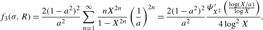 \begin{align} &f_3(\sigma ,R) = \frac {2(1-a^2)^2}{a^2}\sum _{n=1}^{\infty } \frac {nX^{2n}}{1-X^{2n}} \left (\frac {1}{a}\right )^{2n}= \frac {2(1-a^2)^2}{a^2} \frac {\Psi^{\prime} _{X^2}\left ( \frac {\log (X/a)}{\log X}\right )}{4 \log ^2X}, \end{align}
and $\Psi _q$
is the
$\Psi _q$
is the $q$
-digamma function (Salem Reference Salem2012), defined by
$q$
-digamma function (Salem Reference Salem2012), defined by
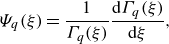 \begin{align} \Psi _q(\xi ) = \frac {1}{\Gamma _q(\xi )}\frac {\mathrm {d}\Gamma _q(\xi )}{\mathrm {d}\xi }, \end{align}
where $\Gamma _q$
is the
$\Gamma _q$
is the $q$
-gamma function (Askey Reference Askey1978). Recall that
$q$
-gamma function (Askey Reference Askey1978). Recall that $a$
and
$a$
and $X$
are given in terms of
$X$
are given in terms of $\sigma$
and
$\sigma$
and $R$
by (3.2). These formulae provide closed forms for the infinite series solutions derived by Sarig et al. (Reference Sarig, Starosvetsky and Gat2016).
$R$
by (3.2). These formulae provide closed forms for the infinite series solutions derived by Sarig et al. (Reference Sarig, Starosvetsky and Gat2016).
The equations of motion for the bubbles are given by (2.8), which reduces to
 \begin{align} f_1(\sigma ,R) \bigl (\overline {\mathcal {U}}_2 -1\bigr )\mathrm {e}^{2\mathrm {i}\phi } -f_2(\sigma ,R) \bigl (\mathcal {U}_1 -1\bigr ) & = -\mathcal {U}_1+\frac { \mathcal {U}_1}{\delta \left |\mathcal {U}_1\right |^{1/3}}, \end{align}
 \begin{align} f_1(\sigma ,R) \bigl (\overline {\mathcal {U}}_1 -1\bigr )\mathrm {e}^{2\mathrm {i}\phi } -f_3(\sigma ,R) \bigl (\mathcal {U}_2 -1\bigr ) & = -R^2\mathcal {U}_2+\frac {R \mathcal {U}_2}{\delta \left |\mathcal {U}_2\right |^{1/3}}. \end{align}
For general $R$
, both
$R$
, both $\sigma$
and
$\sigma$
and $\phi$
vary with time,
$\phi$
vary with time, $t$
, which is made dimensionless using the advective time scale
$t$
, which is made dimensionless using the advective time scale $\hat {R}_1/\hat {U}$
. At each instant, the system (3.16) is solved for
$\hat {R}_1/\hat {U}$
. At each instant, the system (3.16) is solved for $\mathcal {U}_k$
(
$\mathcal {U}_k$
( $k=1,\,2$
), using Newton’s method, and the bubble positions
$k=1,\,2$
), using Newton’s method, and the bubble positions $z_k=x_k+\mathrm {i}y_k$
are then updated using
$z_k=x_k+\mathrm {i}y_k$
are then updated using
 \begin{align} \frac {\mathrm {d}z_k}{\mathrm {d}t}=\mathcal {U}_k. \end{align}
We solve (3.17) using a forward Euler discretisation with a time step of 0.01, which was found to achieve a relative error of approximately $10^{-5}$
in the bubble positions (by comparison with solutions obtained with a smaller time step).
$10^{-5}$
in the bubble positions (by comparison with solutions obtained with a smaller time step).
If the bubbles are identical ( $R=1$
), then (3.2b
) implies that
$R=1$
), then (3.2b
) implies that $X=a^2$
so equations (3.16) are equivalent, and it follows that
$X=a^2$
so equations (3.16) are equivalent, and it follows that $\mathcal {U}_1=\mathcal {U}_2\equiv \mathcal {U}_p$
. Therefore, the two bubbles move at the same velocity, and the values of
$\mathcal {U}_1=\mathcal {U}_2\equiv \mathcal {U}_p$
. Therefore, the two bubbles move at the same velocity, and the values of $\sigma$
and
$\sigma$
and $\phi$
remain fixed for all time, a result that is expected for pairs of identical circular bubbles in a Hele-Shaw cell at low Reynolds number (Happel & Brenner Reference Happel and Brenner2012; Sarig et al. Reference Sarig, Starosvetsky and Gat2016; Green Reference Green2018). The trajectories of non-identical circular bubbles are also expected to be reversible and fore-aft symmetric, which is indeed what our model predicts.
$\phi$
remain fixed for all time, a result that is expected for pairs of identical circular bubbles in a Hele-Shaw cell at low Reynolds number (Happel & Brenner Reference Happel and Brenner2012; Sarig et al. Reference Sarig, Starosvetsky and Gat2016; Green Reference Green2018). The trajectories of non-identical circular bubbles are also expected to be reversible and fore-aft symmetric, which is indeed what our model predicts.
Having established our theoretical model for the motion of a pair of bubbles in a Hele-Shaw cell, we next describe the setup used for our experiments.
4. Experimental methods
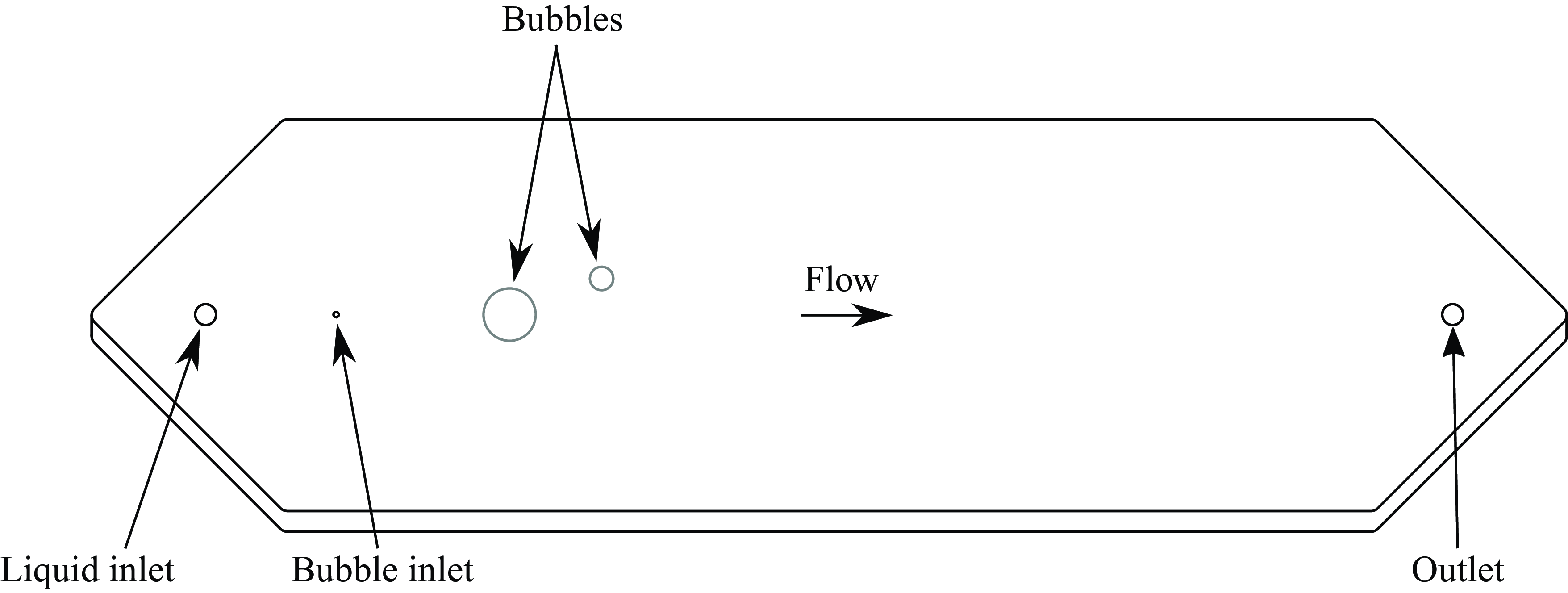
Figure 3. Diagram of the Hele-Shaw cell including bubbles of typical size.
Experiments were performed in a Hele-Shaw cell constructed using two 12.7 mm thick cast acrylic plates. A section shaped like an elongated hexagon was sealed by a gasket along its perimeter, and a uniform distance between the plates was maintained using plastic spacers. The plan view layout of the cell is shown in figure 3.
Flow in the channel was manipulated using a series of circular holes cut into the top plate. Liquid was injected into and removed from the cell through 4 mm diameter holes whose centres were located at opposing vertices of the hexagon. Bubbles were manually introduced using a syringe connected to a 1 mm diameter hole located downstream of the main inlet. The bubble inlet was sealed when not in use to limit fluctuations in pressure and flow rate during measurements. The components of the cell were cleaned with ethanol and distilled water prior to assembly and experiments.
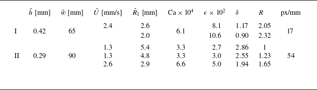
Table 1. Experimental parameters: the channel height $\hat {h}$
, the channel width
$\hat {h}$
, the channel width $\hat {w}$
, the depth-averaged background flow velocity
$\hat {w}$
, the depth-averaged background flow velocity $\hat {U}$
, the effective bubble radius of the smaller bubble
$\hat {U}$
, the effective bubble radius of the smaller bubble $\hat {R}_1$
, the capillary number
$\hat {R}_1$
, the capillary number $\mathrm {Ca} = \hat{\unicode{x03BC}}\hat {U}/\hat {\gamma }$
, the bubble aspect ratio
$\mathrm {Ca} = \hat{\unicode{x03BC}}\hat {U}/\hat {\gamma }$
, the bubble aspect ratio $\epsilon = \hat {h}/2\hat {R}_1$
, the Bretherton parameter
$\epsilon = \hat {h}/2\hat {R}_1$
, the Bretherton parameter $\delta = \mathrm {Ca}^{1/3}/\eta \epsilon$
, the radius ratio
$\delta = \mathrm {Ca}^{1/3}/\eta \epsilon$
, the radius ratio $R$
and image resolution reported in pixels per mm. Parameters are shown for experiments investigating interactions (I) between nearly circular bubbles with an initial offset in the
$R$
and image resolution reported in pixels per mm. Parameters are shown for experiments investigating interactions (I) between nearly circular bubbles with an initial offset in the $y$
-direction as discussed in § 5, and (II) between bubbles in a line parallel to background flow as discussed in § 6.
$y$
-direction as discussed in § 5, and (II) between bubbles in a line parallel to background flow as discussed in § 6.
The viscous liquid used in experiments was silicone oil (Sigma Aldrich, Product No. 317 667). According to information provided by the manufacturer, its kinematic viscosity was $\hat {\nu } = 5\,\rm mm^2s^-{^1}$
, and its dynamic viscosity was
$\hat {\nu } = 5\,\rm mm^2s^-{^1}$
, and its dynamic viscosity was $\hat {\mu } = 4.6\,\rm mPa$
s. The surface tension was measured using the pendant drop method to be
$\hat {\mu } = 4.6\,\rm mPa$
s. The surface tension was measured using the pendant drop method to be $\hat {\gamma } = 18.2\,\rm mN\,m^-{^1}$
. The bubbles were composed of air. Flow was generated by driving oil into the cell at a constant volumetric flow rate,
$\hat {\gamma } = 18.2\,\rm mN\,m^-{^1}$
. The bubbles were composed of air. Flow was generated by driving oil into the cell at a constant volumetric flow rate, $\hat {Q}$
, through the liquid inlet using a syringe pump (Harvard Apparatus, PHD Ultra). Oil ejected from the cell was collected, filtered then reused. Blockage effects due to the presence of the bubbles were not taken into account, and the background flow velocity was estimated to be
$\hat {Q}$
, through the liquid inlet using a syringe pump (Harvard Apparatus, PHD Ultra). Oil ejected from the cell was collected, filtered then reused. Blockage effects due to the presence of the bubbles were not taken into account, and the background flow velocity was estimated to be $\hat {U} = \hat {Q}/\hat {w}\hat {h}$
(where
$\hat {U} = \hat {Q}/\hat {w}\hat {h}$
(where $\hat {w}$
and
$\hat {w}$
and $\hat {h}$
are the dimensional cell width and height). The Reynolds numbers
$\hat {h}$
are the dimensional cell width and height). The Reynolds numbers $\textrm{Re} = 2\hat {U}\hat {R}_1\epsilon ^2/\hat {\nu }$
calculated using the smaller bubble radius ranged from
$\textrm{Re} = 2\hat {U}\hat {R}_1\epsilon ^2/\hat {\nu }$
calculated using the smaller bubble radius ranged from $7.2 \times 10^{-3}$
to
$7.2 \times 10^{-3}$
to $1.7 \times 10^{-2}$
.
$1.7 \times 10^{-2}$
.
Experiments were recorded using a DSLR camera (Nikon) positioned to capture the plan view of the Hele-Shaw cell. The cell was illuminated from above, and a light-absorbing black background was used to enhance contrast. Reflections of light from the bubble interfaces caused the plan view shapes of the bubbles to appear as white outlines. Videos were acquired at 30 frames per second, and calibration was performed using an object of known size in the focal plane.
Table 1 shows a summary of the experiments presented in this work. Experiments were performed to investigate the interactions (I) between two nearly circular bubbles with an initial offset in the $y$
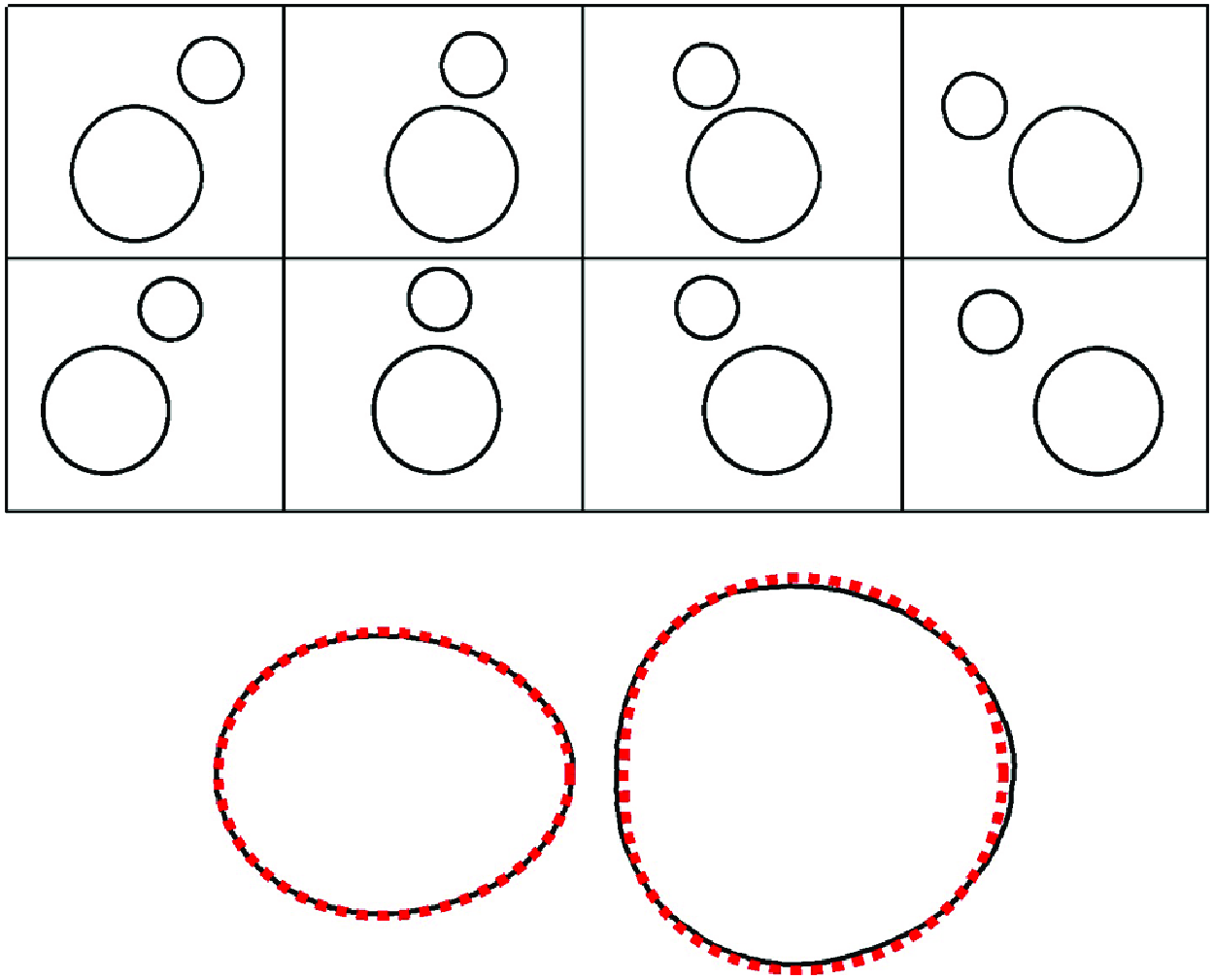
-direction, which exhibit the rollover phenomenon introduced in § 5, and (II) between two bubbles in a line parallel to the background flow, which induce shape deformations in each other as discussed in § 6. The Hele-Shaw cell used to investigate (I) had a rectangular section 19 cm long, and the one used to investigate (II) was 22 cm long. In the rollover experiments (I), the bubbles were slightly flattened in the direction of the flow with aspect ratios typically within 5 % of circularity, which is consistent with the shape perturbations predicted by Wu et al. (Reference Wu, Booth, Griffiths, Howell, Nunes and Stone2024) for isolated bubbles in uniform flow. Thus, they were tracked by fitting ellipses onto their outlines in the images. The bubble velocities were obtained using central finite differences with forward and backward finite differences applied at the two endpoints. In experiments investigating the deformation of two bubbles aligned with the flow (II), bubble shapes were extracted by obtaining an array of points on the closed contour on which the pixel intensity was maximised in grey-scale images. In all cases, the radius of a circle of equivalent area for each bubble was used as the effective radius of the bubble for scaling and further data reduction. We observed that bubbles decreased in size slightly as they travelled downstream, which we attribute to the diffusion of air from the bubble into the silicone oil (Chuan & Yurun Reference Chuan and Yurun2011). Over the course of an experiment, whose typical duration was 15 s, bubbles experienced an average decrease in their effective radius by approximately 2 %. Measurements are reported using the time-averaged bubble size.
$y$
-direction, which exhibit the rollover phenomenon introduced in § 5, and (II) between two bubbles in a line parallel to the background flow, which induce shape deformations in each other as discussed in § 6. The Hele-Shaw cell used to investigate (I) had a rectangular section 19 cm long, and the one used to investigate (II) was 22 cm long. In the rollover experiments (I), the bubbles were slightly flattened in the direction of the flow with aspect ratios typically within 5 % of circularity, which is consistent with the shape perturbations predicted by Wu et al. (Reference Wu, Booth, Griffiths, Howell, Nunes and Stone2024) for isolated bubbles in uniform flow. Thus, they were tracked by fitting ellipses onto their outlines in the images. The bubble velocities were obtained using central finite differences with forward and backward finite differences applied at the two endpoints. In experiments investigating the deformation of two bubbles aligned with the flow (II), bubble shapes were extracted by obtaining an array of points on the closed contour on which the pixel intensity was maximised in grey-scale images. In all cases, the radius of a circle of equivalent area for each bubble was used as the effective radius of the bubble for scaling and further data reduction. We observed that bubbles decreased in size slightly as they travelled downstream, which we attribute to the diffusion of air from the bubble into the silicone oil (Chuan & Yurun Reference Chuan and Yurun2011). Over the course of an experiment, whose typical duration was 15 s, bubbles experienced an average decrease in their effective radius by approximately 2 %. Measurements are reported using the time-averaged bubble size.
5. Bubble rollover
5.1. Observed behaviour
In this section, we consider situations involving two nearly circular bubbles in which the larger bubble is initially far behind the smaller one and offset in the $y$
-direction by a distance less than the sum of the two bubble’s radii, such that
$y$
-direction by a distance less than the sum of the two bubble’s radii, such that $x_1-x_2\gg 1$
and
$x_1-x_2\gg 1$
and $0\lt |y_2-y_1|\lt 1+R$
. As explained in § 2.1, the larger bubble at the rear is expected to travel faster than the bubble at the front (Booth et al. Reference Booth, Griffiths and Howell2023). Thus, the bubbles would collide if they only moved parallel to the background flow. However, for a range of starting positions, we find that the nonlinear hydrodynamic interaction between the bubbles allows them to avoid collision by rotating around one another. Lubrication forces prevent the collision of the nearly circular bubbles in a manner that is analogous to how they cause rigid spheres or cylinders to rotate around and pass each other without contact in shear flow (see, e.g. Arp & Mason Reference Arp and Mason1977b
). As the larger bubble approaches from behind, it continues along a relatively straight trajectory. It overtakes the smaller bubble, which manoeuvres out of the way to let the larger bubble pass.
$0\lt |y_2-y_1|\lt 1+R$
. As explained in § 2.1, the larger bubble at the rear is expected to travel faster than the bubble at the front (Booth et al. Reference Booth, Griffiths and Howell2023). Thus, the bubbles would collide if they only moved parallel to the background flow. However, for a range of starting positions, we find that the nonlinear hydrodynamic interaction between the bubbles allows them to avoid collision by rotating around one another. Lubrication forces prevent the collision of the nearly circular bubbles in a manner that is analogous to how they cause rigid spheres or cylinders to rotate around and pass each other without contact in shear flow (see, e.g. Arp & Mason Reference Arp and Mason1977b
). As the larger bubble approaches from behind, it continues along a relatively straight trajectory. It overtakes the smaller bubble, which manoeuvres out of the way to let the larger bubble pass.
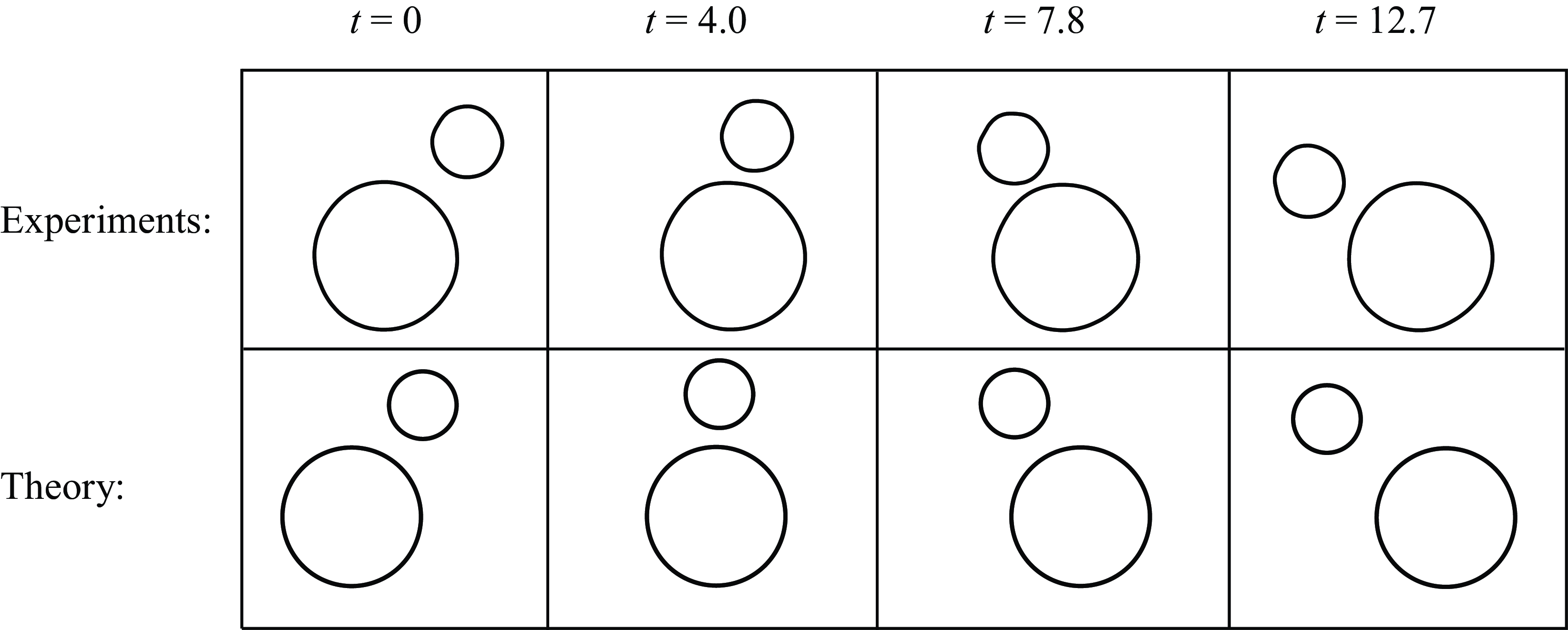
Figure 4. Two-bubble rollover with $\delta =1.17$
and
$\delta =1.17$
and $R=2.05$
at different dimensionless times
$R=2.05$
at different dimensionless times $t = \hat {t}\hat {U}/\hat {R}_1$
. (top) Experimental images are compared with (bottom) simulations of the dimensionless dynamical system (3.17) with the same initial conditions at
$t = \hat {t}\hat {U}/\hat {R}_1$
. (top) Experimental images are compared with (bottom) simulations of the dimensionless dynamical system (3.17) with the same initial conditions at $t=0$
. The background flow is from left to right. Experimental images have been rescaled by the rear bubble radius,
$t=0$
. The background flow is from left to right. Experimental images have been rescaled by the rear bubble radius, $\hat {R}_1 =$
2.6 mm, for comparison with the theory.
$\hat {R}_1 =$
2.6 mm, for comparison with the theory.
In figure 4, we show experimental images demonstrating this rollover effect for a system of two approximately circular bubbles with $\delta =1.17$
and
$\delta =1.17$
and $R=2.05$
(see movie 1 provided in the Supplementary Material). The larger bubble catches up to the smaller one, which evades contact by rolling over the larger one. In the lower plots, we demonstrate good qualitative agreement with solutions of the dynamical system (3.17) for the same parameter values and initial conditions. Movies 2–7 in the Supplementary Material show additional instances of the two-bubble rollover phenomenon, serving as evidence that it is reproducible for various combinations of bubble sizes and initial conditions.
$R=2.05$
(see movie 1 provided in the Supplementary Material). The larger bubble catches up to the smaller one, which evades contact by rolling over the larger one. In the lower plots, we demonstrate good qualitative agreement with solutions of the dynamical system (3.17) for the same parameter values and initial conditions. Movies 2–7 in the Supplementary Material show additional instances of the two-bubble rollover phenomenon, serving as evidence that it is reproducible for various combinations of bubble sizes and initial conditions.
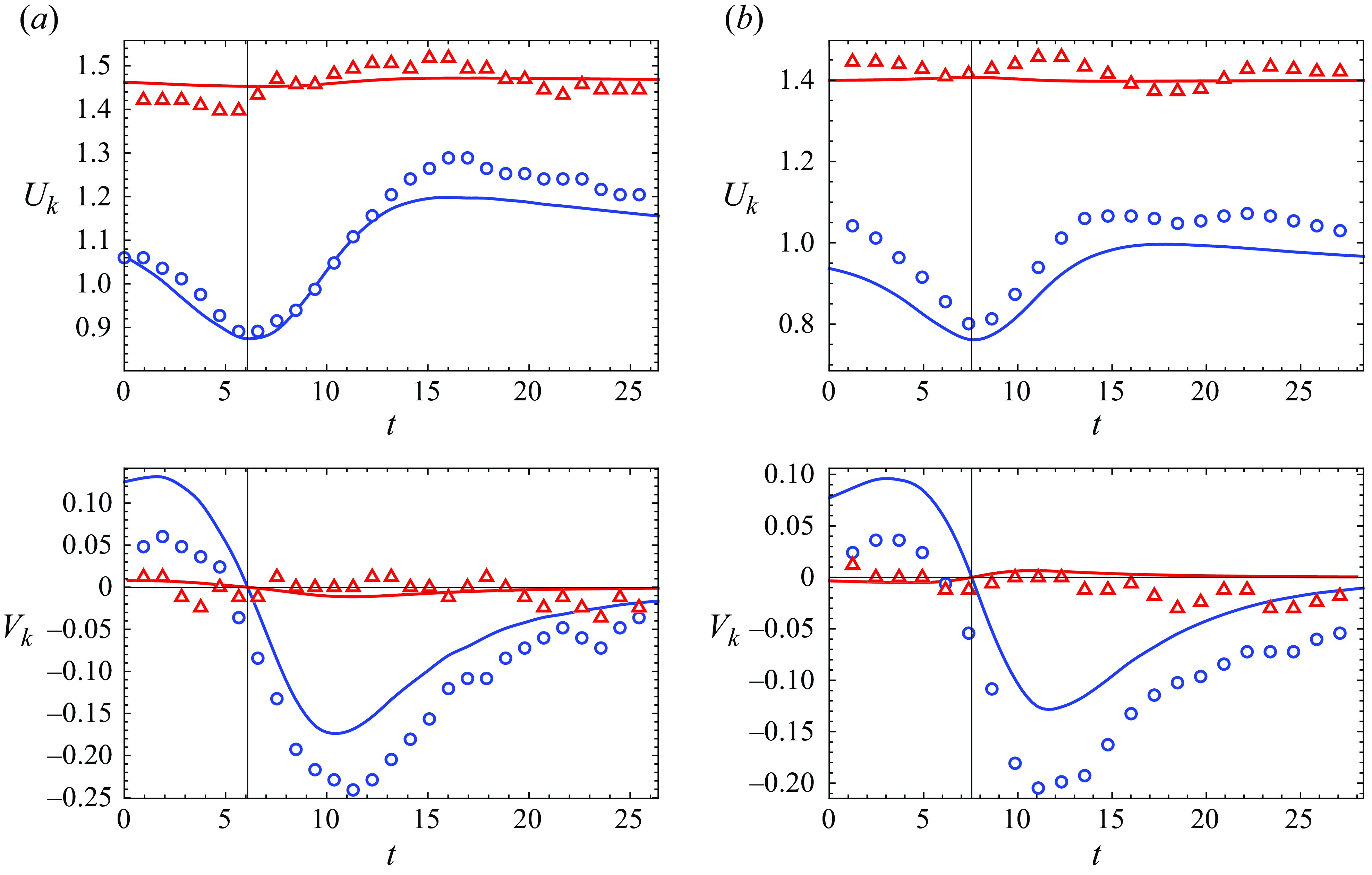
Figure 5. The instantaneous bubble velocity components $(U_k,V_k)$
(top and bottom, respectively) versus dimensionless time
$(U_k,V_k)$
(top and bottom, respectively) versus dimensionless time $t$
for (a)
$t$
for (a) $\delta =1.17$
and
$\delta =1.17$
and $R=2.05$
, (b)
$R=2.05$
, (b) $\delta =0.90$
and
$\delta =0.90$
and $R=2.32$
. Solid lines show theoretical predictions and points show experimental data. The bubble of unit dimensionless radius (
$R=2.32$
. Solid lines show theoretical predictions and points show experimental data. The bubble of unit dimensionless radius ( $k=1$
) is shown in blue (circles), and the bubble of radius
$k=1$
) is shown in blue (circles), and the bubble of radius $R$
(
$R$
( $k=2$
) is shown in red (triangles). In each plot, the time at which
$k=2$
) is shown in red (triangles). In each plot, the time at which $x_1=x_2$
is shown with a vertical line. Error bars are comparable to the size of the markers and are thus omitted.
$x_1=x_2$
is shown with a vertical line. Error bars are comparable to the size of the markers and are thus omitted.
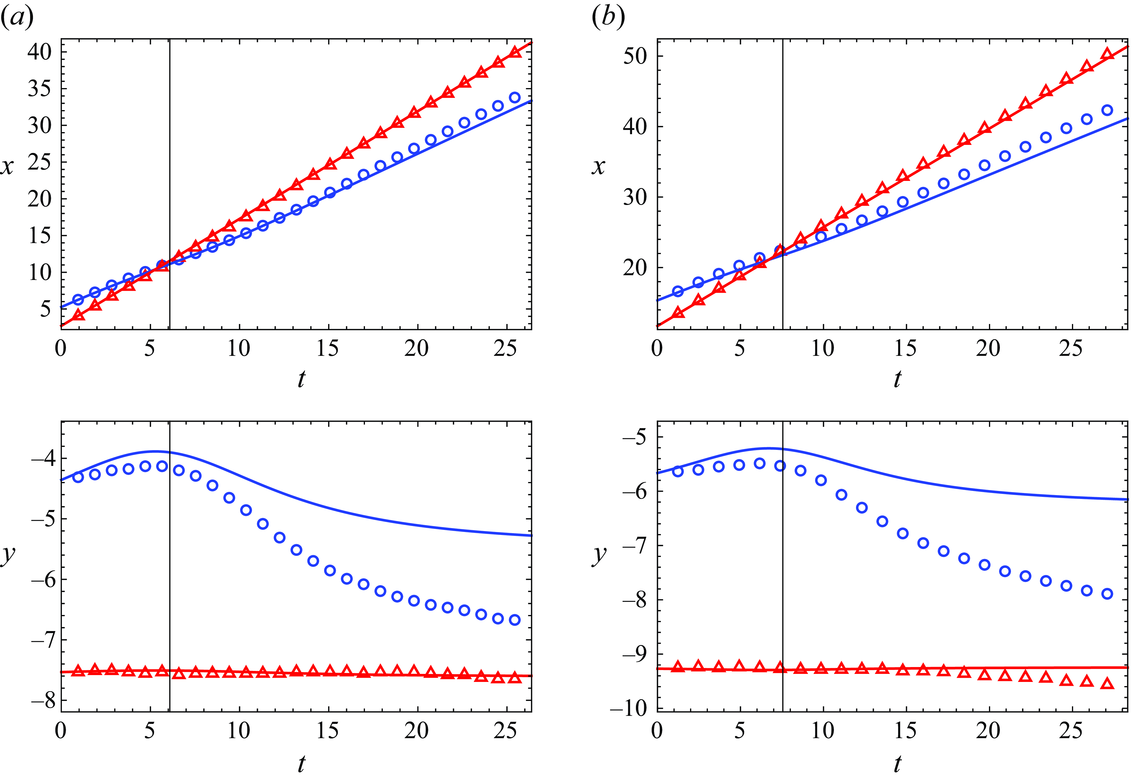
Figure 6. The positions of the bubble centres $(x,y)$
(top and bottom, respectively) versus dimensionless time
$(x,y)$
(top and bottom, respectively) versus dimensionless time $t$
for (a)
$t$
for (a) $\delta =1.17$
and
$\delta =1.17$
and $R=2.05$
, (b)
$R=2.05$
, (b) $\delta =0.90$
and
$\delta =0.90$
and $R=2.32$
. Solid lines show theoretical predictions, and points show experimental data. The bubble of unit radius (
$R=2.32$
. Solid lines show theoretical predictions, and points show experimental data. The bubble of unit radius ( $k=1$
) is shown in blue (circles), and the bubble of radius
$k=1$
) is shown in blue (circles), and the bubble of radius $R$
(
$R$
( $k=2$
) is shown in red (triangles). In each plot, the time at which
$k=2$
) is shown in red (triangles). In each plot, the time at which $x_1=x_2$
is shown with a vertical line. Error bars are comparable to the size of the markers and are thus omitted.
$x_1=x_2$
is shown with a vertical line. Error bars are comparable to the size of the markers and are thus omitted.

Figure 7. Trajectories for the two-bubble dynamical system (3.17) in the reference frame of the smaller bubble, with (a) $\delta =1.17$
and
$\delta =1.17$
and $R=2.05$
, (b)
$R=2.05$
, (b) $\delta =0.90$
and
$\delta =0.90$
and $R=2.32$
. The blue vectors show the predicted trajectories of the centre of the larger bubble relative to the smaller one, and the red points show the experimentally measured bubble positions. Error bars are comparable to the size of the markers and are thus omitted. Any trajectories entering the solid grey region
$R=2.32$
. The blue vectors show the predicted trajectories of the centre of the larger bubble relative to the smaller one, and the red points show the experimentally measured bubble positions. Error bars are comparable to the size of the markers and are thus omitted. Any trajectories entering the solid grey region $|z_2-z_1| \leqslant (1+R)$
are such that the two bubbles will collide. The solid black region
$|z_2-z_1| \leqslant (1+R)$
are such that the two bubbles will collide. The solid black region $|z_2-z_1| \leqslant 1$
represents the smaller bubble.
$|z_2-z_1| \leqslant 1$
represents the smaller bubble.
In figure 5, the instantaneous bubble velocity components $(U_k,V_k)$
are plotted for the same experiment as shown in figure 4 and for another example in which
$(U_k,V_k)$
are plotted for the same experiment as shown in figure 4 and for another example in which $\delta =0.90$
and
$\delta =0.90$
and $R=2.32$
(see movie 2 provided in the Supplementary Material). The model predicts that the smaller bubble decelerates in the
$R=2.32$
(see movie 2 provided in the Supplementary Material). The model predicts that the smaller bubble decelerates in the $x$
-direction as the large bubble approaches from behind, while also translating in the
$x$
-direction as the large bubble approaches from behind, while also translating in the $y$
-direction such that
$y$
-direction such that $|y_2-y_1|$
is increasing. The time at which the pair of bubbles is aligned perpendicularly to the background flow (i.e. when
$|y_2-y_1|$
is increasing. The time at which the pair of bubbles is aligned perpendicularly to the background flow (i.e. when $x_1=x_2$
) coincides with when the axial velocity of the smaller bubble,
$x_1=x_2$
) coincides with when the axial velocity of the smaller bubble, $U_1$
, reaches a minimum and when
$U_1$
, reaches a minimum and when $V_1=V_2=0$
. We observe reasonable agreement between theory and experiment. However, in experiments, the velocity components
$V_1=V_2=0$
. We observe reasonable agreement between theory and experiment. However, in experiments, the velocity components $U_1$
and
$U_1$
and $V_1$
of the smaller bubble are generally biased to reduce the distance between the bubble centres.
$V_1$
of the smaller bubble are generally biased to reduce the distance between the bubble centres.
In figure 6, we compare the experimental and theoretical results for the $(x,y)$
-positions of the bubble centres. In both cases, we observe that the motion of the larger bubble is largely unaffected by the interaction while the smaller bubble is displaced in the
$(x,y)$
-positions of the bubble centres. In both cases, we observe that the motion of the larger bubble is largely unaffected by the interaction while the smaller bubble is displaced in the $y$
-direction such that the bubbles avoid contact as the larger one passes. The final distance in the
$y$
-direction such that the bubbles avoid contact as the larger one passes. The final distance in the $y$
-direction between the bubbles in experiments is significantly smaller than what is theoretically predicted. The bubbles also become slightly closer in the
$y$
-direction between the bubbles in experiments is significantly smaller than what is theoretically predicted. The bubbles also become slightly closer in the $x$
-direction in experiments as compared with theory. The small discrepancies between the theoretical and experimental velocities shown in figure 5 accumulate over time and lead to noticeable differences between the theoretical and experimental bubble trajectories.
$x$
-direction in experiments as compared with theory. The small discrepancies between the theoretical and experimental velocities shown in figure 5 accumulate over time and lead to noticeable differences between the theoretical and experimental bubble trajectories.
Finally, in figure 7 we plot the trajectories of the centre of the larger bubble relative to that of the smaller one (i.e. $z_2-z_1$
) calculated using (3.17). Any trajectory entering the solid grey region
$z_2-z_1$
) calculated using (3.17). Any trajectory entering the solid grey region $|z_2-z_1|\leqslant 1+R$
corresponds to a collision between the bubbles. Points extracted from the experiments are superimposed on the theoretically determined bubble trajectories. We observe that in experiments, the larger bubble initially follows a trajectory, then departs from that trajectory when the two bubbles are close. This departure is likely to be due to interactions between the bubbles that are not included in the model. Finally, as the bubbles separate, the larger bubble once again closely follows a trajectory, albeit a different trajectory from the one on which the bubble started.
$|z_2-z_1|\leqslant 1+R$
corresponds to a collision between the bubbles. Points extracted from the experiments are superimposed on the theoretically determined bubble trajectories. We observe that in experiments, the larger bubble initially follows a trajectory, then departs from that trajectory when the two bubbles are close. This departure is likely to be due to interactions between the bubbles that are not included in the model. Finally, as the bubbles separate, the larger bubble once again closely follows a trajectory, albeit a different trajectory from the one on which the bubble started.
While the $x$
-positions of the bubble centres are well captured by the theory, there is a significant disagreement between the predicted and observed
$x$
-positions of the bubble centres are well captured by the theory, there is a significant disagreement between the predicted and observed $y$
-positions of the smaller bubble during and after the rollover (see figure 6). In the experiments, the smaller bubble appears to be entrained behind the larger bubble such that the distances between their centres in both the
$y$
-positions of the smaller bubble during and after the rollover (see figure 6). In the experiments, the smaller bubble appears to be entrained behind the larger bubble such that the distances between their centres in both the $x$
- and
$x$
- and $y$
-directions are smaller than the corresponding theoretical trajectories. This process breaks the fore–aft symmetry that is predicted by (3.17), and indeed which would be expected in Stokes flow for circular bubbles. However, as noted in § 4, there are perturbations to the bubble shape due to the background flow, which also happen to be fore–aft asymmetric due to the differences between the advancing and retreating menisci (Wu et al. Reference Wu, Booth, Griffiths, Howell, Nunes and Stone2024). Deformations due to interactions between bubbles are known to cause asymmetric trajectories for unconfined bubbles rising due to buoyancy. Experiments and numerical simulations performed at low Reynolds numbers have shown that a smaller bubble tends to align itself behind a larger bubble and even accelerate towards it so that the two bubbles collide, all while both bubbles undergo significant deformations (Manga & Stone Reference Manga and Stone1993, Reference Manga and Stone1995). It is possible that small inertial effects also play a role: experiments and numerical simulations have shown that a deformable bubble rising due to buoyancy behind another one tends to get drawn into the wake of the latter (Crabtree & Bridgwater Reference Crabtree and Bridgwater1971; Katz & Meneveau Reference Katz and Meneveau1996; Bunner & Tryggvason Reference Bunner and Tryggvason2003; Huisman, Ern & Roig Reference Huisman, Ern and Roig2012). In § 6, we investigate the deviations in the bubble shape of two bubbles in a line parallel to the background flow.
$y$
-directions are smaller than the corresponding theoretical trajectories. This process breaks the fore–aft symmetry that is predicted by (3.17), and indeed which would be expected in Stokes flow for circular bubbles. However, as noted in § 4, there are perturbations to the bubble shape due to the background flow, which also happen to be fore–aft asymmetric due to the differences between the advancing and retreating menisci (Wu et al. Reference Wu, Booth, Griffiths, Howell, Nunes and Stone2024). Deformations due to interactions between bubbles are known to cause asymmetric trajectories for unconfined bubbles rising due to buoyancy. Experiments and numerical simulations performed at low Reynolds numbers have shown that a smaller bubble tends to align itself behind a larger bubble and even accelerate towards it so that the two bubbles collide, all while both bubbles undergo significant deformations (Manga & Stone Reference Manga and Stone1993, Reference Manga and Stone1995). It is possible that small inertial effects also play a role: experiments and numerical simulations have shown that a deformable bubble rising due to buoyancy behind another one tends to get drawn into the wake of the latter (Crabtree & Bridgwater Reference Crabtree and Bridgwater1971; Katz & Meneveau Reference Katz and Meneveau1996; Bunner & Tryggvason Reference Bunner and Tryggvason2003; Huisman, Ern & Roig Reference Huisman, Ern and Roig2012). In § 6, we investigate the deviations in the bubble shape of two bubbles in a line parallel to the background flow.
5.2. Do the bubbles collide?
5.2.1. Conditions for a bubble collision
In § 5.1 we found that the bubbles can avoid colliding by rolling over one another. By analysing the dynamical system (3.17), we can predict when or if the bubble rollover effect will occur. We note that the following analysis of bubble–bubble collisions is conducted within the context of the Hele-Shaw model. The Hele-Shaw model will break down when the bubbles are close to contact, in which case a three-dimensional analysis would be needed to achieve a complete description of the dynamics.
At each instant in time, (3.16) determines $\mathcal {U}_1$
and
$\mathcal {U}_1$
and $\mathcal {U}_2$
as functions of
$\mathcal {U}_2$
as functions of $\sigma$
and
$\sigma$
and $\phi$
. We can then update
$\phi$
. We can then update $\sigma$
and
$\sigma$
and $\phi$
using
$\phi$
using $\mathcal {U}_2-\mathcal {U}_1= (\dot {\sigma }+\mathrm {i}\sigma \dot {\phi } )\mathrm {e}^{\mathrm {i}\phi }$
(where the dot represents differentiation with respect to
$\mathcal {U}_2-\mathcal {U}_1= (\dot {\sigma }+\mathrm {i}\sigma \dot {\phi } )\mathrm {e}^{\mathrm {i}\phi }$
(where the dot represents differentiation with respect to $t$
). In figure 8, we plot the phase space showing the resulting trajectories of the larger bubble relative to the smaller one, i.e.
$t$
). In figure 8, we plot the phase space showing the resulting trajectories of the larger bubble relative to the smaller one, i.e. $z_2-z_1=\sigma \mathrm {e}^{\mathrm {i}\phi }$
. In this figure, we take
$z_2-z_1=\sigma \mathrm {e}^{\mathrm {i}\phi }$
. In this figure, we take $R=2$
for illustration. The solid grey region,
$R=2$
for illustration. The solid grey region, $1\lt |z_2-z_1|\leqslant (1+R)$
, corresponds to the region of intersection between the bubbles. The rollover effect occurs on any trajectory that starts from
$1\lt |z_2-z_1|\leqslant (1+R)$
, corresponds to the region of intersection between the bubbles. The rollover effect occurs on any trajectory that starts from $x_1-x_2\gg 1$
with
$x_1-x_2\gg 1$
with $0\lt |y_2-y_1|\lt 1+R$
and that does not enter the solid grey region, and the likelihood of observing the effect depends strongly on the value of
$0\lt |y_2-y_1|\lt 1+R$
and that does not enter the solid grey region, and the likelihood of observing the effect depends strongly on the value of $\delta$
. In figure 8(a), we show a case where
$\delta$
. In figure 8(a), we show a case where $\delta$
is large, and all suitable initial conditions satisfying the inequalities stated above will give rise to the rollover effect. In this case, the bubbles repel each other so strongly that collision between the bubbles is impossible. On the other hand, in figure 8(b), we show that a smaller value of
$\delta$
is large, and all suitable initial conditions satisfying the inequalities stated above will give rise to the rollover effect. In this case, the bubbles repel each other so strongly that collision between the bubbles is impossible. On the other hand, in figure 8(b), we show that a smaller value of $\delta$
leads to much weaker interaction between the bubbles, such that the trajectories remain almost parallel to the flow. In this case, the rollover effect can occur only for a very narrow band of initial conditions, and we are much more likely to observe the bubbles colliding with each other. To understand the underlying physical mechanisms, we recall that
$\delta$
leads to much weaker interaction between the bubbles, such that the trajectories remain almost parallel to the flow. In this case, the rollover effect can occur only for a very narrow band of initial conditions, and we are much more likely to observe the bubbles colliding with each other. To understand the underlying physical mechanisms, we recall that $\delta$
is a dimensionless parameter that compares the relative magnitudes of the viscous pressure and of the Bretherton pressure, and that in this system
$\delta$
is a dimensionless parameter that compares the relative magnitudes of the viscous pressure and of the Bretherton pressure, and that in this system $\delta$
is defined using the radius of the smaller bubble, whose motion is essential to successful rollover. As
$\delta$
is defined using the radius of the smaller bubble, whose motion is essential to successful rollover. As $\delta$
increases, the magnitude of the viscous pressure dominates that of the Bretherton pressure, so the motion of the smaller bubble is less hindered by the Bretherton drag, and collision is less likely.
$\delta$
increases, the magnitude of the viscous pressure dominates that of the Bretherton pressure, so the motion of the smaller bubble is less hindered by the Bretherton drag, and collision is less likely.

Figure 8. Trajectories for the two-bubble dynamical system (3.17) in the reference frame of the smaller bubble, with $R=2$
and (a)
$R=2$
and (a) $\delta =5$
, (b)
$\delta =5$
, (b) $\delta =1/2$
. Any trajectories entering the solid grey region
$\delta =1/2$
. Any trajectories entering the solid grey region $|z_2-z_1| \leqslant (1+R)$
are such that the two bubbles will collide. Stationary points are shown in red. The solid black region
$|z_2-z_1| \leqslant (1+R)$
are such that the two bubbles will collide. Stationary points are shown in red. The solid black region $|z_2-z_1| \leqslant 1$
represents the smaller bubble.
$|z_2-z_1| \leqslant 1$
represents the smaller bubble.
In this section, we consider conditions under which the bubbles will collide. First, we observe that there are stationary points (saddle points, located at $\phi = 0$
and
$\phi = 0$
and $\phi =\pi$
, shown in red) in figure 8(a) but not in figure 8(b). The existence of such stationary points outside of the solid grey region as in figure 8(a) implies that two aligned bubbles (i.e. with
$\phi =\pi$
, shown in red) in figure 8(a) but not in figure 8(b). The existence of such stationary points outside of the solid grey region as in figure 8(a) implies that two aligned bubbles (i.e. with $y_1=y_2$
) will never collide. The stable manifolds of the two saddle points coincide with the horizontal axis,
$y_1=y_2$
) will never collide. The stable manifolds of the two saddle points coincide with the horizontal axis, $y_1-y_2 = 0$
, so a point on the horizontal axis also lies on the stable manifold of one of the stationary points. Therefore trajectories beginning on the horizontal axis converge to a stationary point without entering the solid grey region. Furthermore, we find that, in figure 8(a), the trajectories on the surface
$y_1-y_2 = 0$
, so a point on the horizontal axis also lies on the stable manifold of one of the stationary points. Therefore trajectories beginning on the horizontal axis converge to a stationary point without entering the solid grey region. Furthermore, we find that, in figure 8(a), the trajectories on the surface $|z_2-z_1|=1+R$
with
$|z_2-z_1|=1+R$
with $x_2\gt x_1$
(the larger bubble in front) are directed inwards (into the solid grey region) and for
$x_2\gt x_1$
(the larger bubble in front) are directed inwards (into the solid grey region) and for $x_2\lt x_1$
are directed outwards. In this case, bubbles may only collide if they are initially close to each other, and the larger bubble is ahead of the smaller one when the collision occurs. The reverse is true in figure 8(b), in which the surface
$x_2\lt x_1$
are directed outwards. In this case, bubbles may only collide if they are initially close to each other, and the larger bubble is ahead of the smaller one when the collision occurs. The reverse is true in figure 8(b), in which the surface $|z_2-z_1|=1+R$
is entirely outside of the separatrix connecting the two stationary points.
$|z_2-z_1|=1+R$
is entirely outside of the separatrix connecting the two stationary points.
Motivated by these observations, we examine the following two conditions on the flow:
-
(i) The stationary points of the dynamical system (3.17) in the reference frame of the smaller bubble are in the region $|z_2-z_1|\geqslant 1+R$
.
$|z_2-z_1|\geqslant 1+R$
. -
(ii) In a neighbourhood of
$x_1=x_2$
, the trajectories point into the region
$|z_2-z_1|\leqslant 1+R$
for
$x_2\gt x_1$
and out of the region
$|z_2-z_1|\leqslant 1+R$
for
$x_2\lt x_1$
.


In § 5.2.2 and § 5.2.3, for each condition $k\in \{1,2\}$
, we will find a critical minimum value of
$k\in \{1,2\}$
, we will find a critical minimum value of $\delta = \delta _k(R)$
. Then, for
$\delta = \delta _k(R)$
. Then, for $\delta \lt \delta _1$
, we argue that there is always a range of initial conditions with
$\delta \lt \delta _1$
, we argue that there is always a range of initial conditions with $x_1-x_2\gg 1$
and
$x_1-x_2\gg 1$
and $|y_2-y_1|\lt 1+R$
such that the bubbles collide (including the case
$|y_2-y_1|\lt 1+R$
such that the bubbles collide (including the case $y_2=y_1$
where the bubbles are aligned). On the other hand, for
$y_2=y_1$
where the bubbles are aligned). On the other hand, for $\delta \gt \delta _2$
, it is impossible for bubbles that start far apart in the
$\delta \gt \delta _2$
, it is impossible for bubbles that start far apart in the $x$
-direction to collide, regardless of their initial transverse separation.
$x$
-direction to collide, regardless of their initial transverse separation.
Note that there exists a third critical value of $\delta =\delta _c(R)$
satisfying
$\delta =\delta _c(R)$
satisfying $\delta _1\leqslant \delta _c\leqslant \delta _2$
, at which the separatrix connecting the two stationary points is tangent to
$\delta _1\leqslant \delta _c\leqslant \delta _2$
, at which the separatrix connecting the two stationary points is tangent to $|z_2-z_1|=1+R$
. This critical value provides a sharp bound on
$|z_2-z_1|=1+R$
. This critical value provides a sharp bound on $\delta$
above which collision between two bubbles that are initially well separated in the
$\delta$
above which collision between two bubbles that are initially well separated in the $x$
-direction (the direction of the background flow) is impossible. However,
$x$
-direction (the direction of the background flow) is impossible. However, $\delta _c$
is delicate to compute numerically as it depends on the global properties of the flow whereas, as we will show, the critical values
$\delta _c$
is delicate to compute numerically as it depends on the global properties of the flow whereas, as we will show, the critical values $\delta _1$
and
$\delta _1$
and $\delta _2$
can be determined from purely local information about the normal velocity
$\delta _2$
can be determined from purely local information about the normal velocity $U_n$
at the collision boundary
$U_n$
at the collision boundary $|z_1-z_2|=1+R$
.
$|z_1-z_2|=1+R$
.
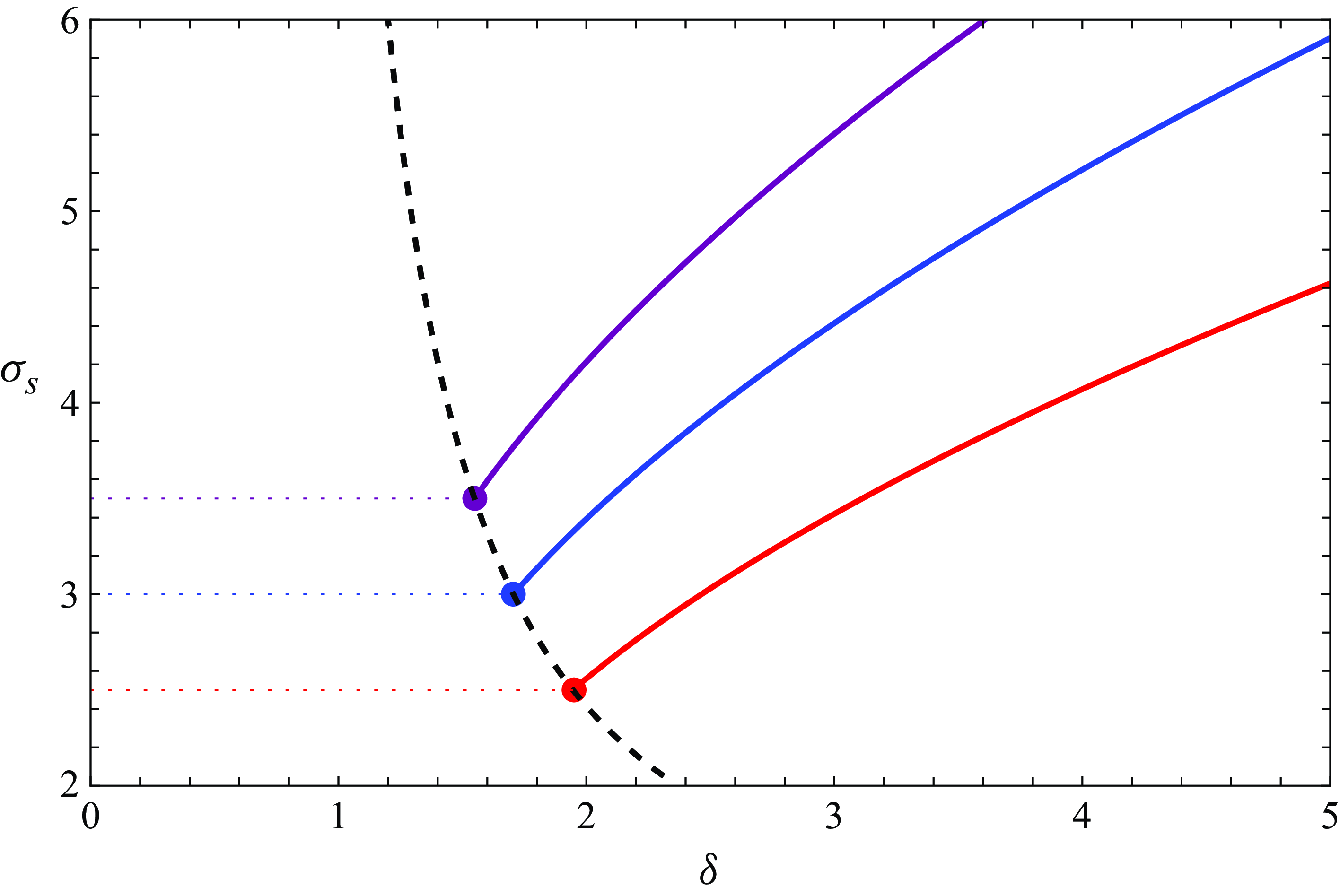
Figure 9. Position of the stationary point, $\sigma _s$
, as a function of the Bretherton parameter,
$\sigma _s$
, as a function of the Bretherton parameter, $\delta$
, for radius ratios
$\delta$
, for radius ratios $R = 1.5$
(red), 2 (blue), 2.5 (purple). The dashed black curve shows where
$R = 1.5$
(red), 2 (blue), 2.5 (purple). The dashed black curve shows where $\sigma _s=1+R$
.
$\sigma _s=1+R$
.
5.2.2. Condition i: stationary points
If this condition is satisfied, then two aligned bubbles will never collide. By analysing (3.16), we can find the stationary points by solving for $\mathcal {U}_1=\mathcal {U}_2\equiv \mathcal {U}$
and for
$\mathcal {U}_1=\mathcal {U}_2\equiv \mathcal {U}$
and for $(\sigma ,\phi )\equiv (\sigma _s,\phi _s)$
at a fixed
$(\sigma ,\phi )\equiv (\sigma _s,\phi _s)$
at a fixed $\delta$
. Since each
$\delta$
. Since each $f_k$
in (3.14) is real, by symmetry we find that
$f_k$
in (3.14) is real, by symmetry we find that $\mathcal {U}=U\in \mathbb {R}$
and
$\mathcal {U}=U\in \mathbb {R}$
and $\phi _s =0$
or
$\phi _s =0$
or $\pi$
. We focus on the case
$\pi$
. We focus on the case $\phi _s=0$
since by symmetry the stationary points are at
$\phi _s=0$
since by symmetry the stationary points are at $(\pm \sigma _s,0)$
. Thus, for given
$(\pm \sigma _s,0)$
. Thus, for given $\delta$
and
$\delta$
and $R$
we find
$R$
we find $U$
and
$U$
and $\sigma _s$
by solving the nonlinear algebraic equations
$\sigma _s$
by solving the nonlinear algebraic equations
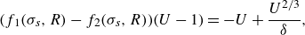 \begin{align} \quad \bigl (f_1(\sigma _s,R)-f_2(\sigma _s,R)\bigr )(U-1)&=-U+\frac {U^{2/3}}{\delta }, \end{align}
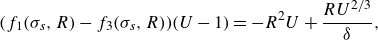 \begin{align} \bigl (f_1(\sigma _s,R)-f_3(\sigma _s,R)\bigr )(U-1)&=-R^2U+\frac {R U^{2/3}}{\delta } ,\end{align}
numerically, using Newton’s method.
The position of the stationary point, $\sigma _s$
, is plotted as a function of the Bretherton parameter,
$\sigma _s$
, is plotted as a function of the Bretherton parameter, $\delta$
, in figure 9. The black dashed curve shows where
$\delta$
, in figure 9. The black dashed curve shows where $\sigma _s=1+R$
. For each fixed value of
$\sigma _s=1+R$
. For each fixed value of $R$
we observe that, for suitably small
$R$
we observe that, for suitably small $\delta$
, there are no stationary points in the region
$\delta$
, there are no stationary points in the region $|z_2-z_1|\geqslant 1+R$
. As
$|z_2-z_1|\geqslant 1+R$
. As $\delta$
is increased, there exists a first value
$\delta$
is increased, there exists a first value $\delta = \delta _1(R)$
at which a stationary point appears at
$\delta = \delta _1(R)$
at which a stationary point appears at $\sigma _s = 1+R$
. Then, for
$\sigma _s = 1+R$
. Then, for $\delta \gt \delta _1$
,
$\delta \gt \delta _1$
, $\sigma _s$
is a monotonically increasing function of
$\sigma _s$
is a monotonically increasing function of $\delta$
.
$\delta$
.
We can find $\delta _1(R)$
by substituting
$\delta _1(R)$
by substituting $\sigma _s=1+R$
in (5.1) and solving for
$\sigma _s=1+R$
in (5.1) and solving for $U$
and
$U$
and $\delta _1$
; the details of this calculation may be found in Appendix A. We plot
$\delta _1$
; the details of this calculation may be found in Appendix A. We plot $\delta _1$
as a function of the bubble radius ratio,
$\delta _1$
as a function of the bubble radius ratio, $R$
, in figure 10. We observe that
$R$
, in figure 10. We observe that $\delta _1$
is a monotonically decreasing function of
$\delta _1$
is a monotonically decreasing function of $R$
, which means that for larger values of
$R$
, which means that for larger values of $R$
the stationary points are present for smaller values of
$R$
the stationary points are present for smaller values of $\delta$
. We also observe that, as
$\delta$
. We also observe that, as $R\rightarrow 1^+$
,
$R\rightarrow 1^+$
, $\delta _1(R)$
tends to a finite value that is approximately
$\delta _1(R)$
tends to a finite value that is approximately $2.37$
.
$2.37$
.
In figure 11(a), we plot the phase space showing the resulting trajectories of the larger bubble relative to the smaller bubble with $R=2$
for
$R=2$
for $\delta =\delta _1(2)$
. We observe that the stationary points of the system occur on the real axis at
$\delta =\delta _1(2)$
. We observe that the stationary points of the system occur on the real axis at $\sigma _s=1+R$
(shown by red points); however, there are still trajectories that enter the solid grey region
$\sigma _s=1+R$
(shown by red points); however, there are still trajectories that enter the solid grey region $|z_2-z_1|\leqslant 1+R$
. Hence the bubbles can still collide.
$|z_2-z_1|\leqslant 1+R$
. Hence the bubbles can still collide.


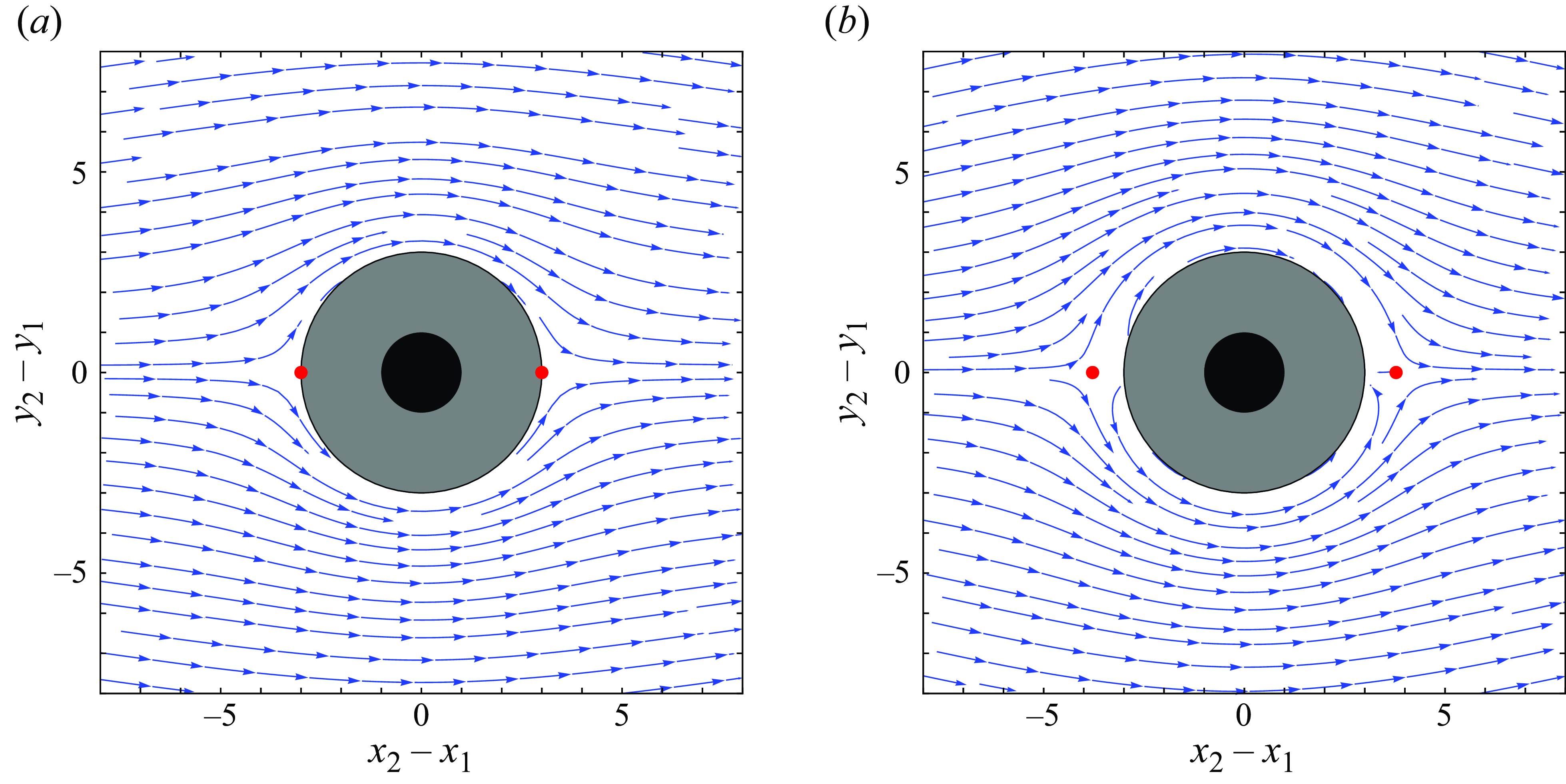
Figure 11. Trajectories for the two-bubble dynamical system (3.17) in the frame of the smaller bubble, with $R=2$
and (a)
$R=2$
and (a) $\delta =\delta _1(2)$
, at which the stationary points (shown as red points) lie on the surface
$\delta =\delta _1(2)$
, at which the stationary points (shown as red points) lie on the surface $|z_2-z_1| =1+R$
, (b)
$|z_2-z_1| =1+R$
, (b) $\delta =\delta _2(2)$
, above which the separatrix encloses the region
$\delta =\delta _2(2)$
, above which the separatrix encloses the region $|z_2-z_1| \lt 1+R$
(solid grey fill). The solid black region
$|z_2-z_1| \lt 1+R$
(solid grey fill). The solid black region $|z_2-z_1| \leqslant 1$
represents the smaller bubble.
$|z_2-z_1| \leqslant 1$
represents the smaller bubble.
5.2.3. Condition ii: normal velocity
Condition ii concerns the sign of the normal relative velocity of the two bubbles in a neighbourhood of the two points where $z_2-z_1=\pm \mathrm {i}(1+R)$
. When this condition is satisfied, the only trajectories that result in a collision of the bubbles are ones in which the bubbles are initially close to one another, and collisions always occur when the larger bubble is ahead of the smaller bubble. If the larger bubble is initially behind the smaller one, the bubbles will rotate around one another before colliding. We define the normal velocity by
$z_2-z_1=\pm \mathrm {i}(1+R)$
. When this condition is satisfied, the only trajectories that result in a collision of the bubbles are ones in which the bubbles are initially close to one another, and collisions always occur when the larger bubble is ahead of the smaller bubble. If the larger bubble is initially behind the smaller one, the bubbles will rotate around one another before colliding. We define the normal velocity by $U_n = (\boldsymbol {U}_2-\boldsymbol {U}_1)\boldsymbol {\cdot } \boldsymbol {n}$
, where here
$U_n = (\boldsymbol {U}_2-\boldsymbol {U}_1)\boldsymbol {\cdot } \boldsymbol {n}$
, where here $\boldsymbol {n}$
is the outward unit normal of the smaller bubble at the point where the bubbles are touching. When the separatrix encloses the region
$\boldsymbol {n}$
is the outward unit normal of the smaller bubble at the point where the bubbles are touching. When the separatrix encloses the region $|z_2-z_1|\leqslant 1+R$
, we have
$|z_2-z_1|\leqslant 1+R$
, we have $U_n\gt 0$
for
$U_n\gt 0$
for $x_2\lt x_1$
, meaning the bubbles separate when the larger bubble is behind, and
$x_2\lt x_1$
, meaning the bubbles separate when the larger bubble is behind, and $U_n\lt 0$
for
$U_n\lt 0$
for $x_2\gt x_1$
, meaning the bubbles collide when the larger bubble is ahead. For condition ii, we find the value of
$x_2\gt x_1$
, meaning the bubbles collide when the larger bubble is ahead. For condition ii, we find the value of $\delta$
at which
$\delta$
at which $U_n$
is stationary at
$U_n$
is stationary at $x_1=x_2$
, i.e.,
$x_1=x_2$
, i.e., $\partial U_n/\partial \phi =0$
at
$\partial U_n/\partial \phi =0$
at $\sigma =1+R$
,
$\sigma =1+R$
, $\phi =\pm \pi /2$
. The details of the calculation can be found in Appendix A.
$\phi =\pm \pi /2$
. The details of the calculation can be found in Appendix A.
We plot $\delta _2$
as a function of the bubble radius ratio,
$\delta _2$
as a function of the bubble radius ratio, $R$
, in figure 10. We observe that
$R$
, in figure 10. We observe that $\delta _2(R)$
is a monotonically decreasing function of
$\delta _2(R)$
is a monotonically decreasing function of $R$
. We also observe that as
$R$
. We also observe that as $R\rightarrow 1^+$
,
$R\rightarrow 1^+$
, $\delta _2(R)$
tends to a finite value
$\delta _2(R)$
tends to a finite value $\delta ^*\approx 3.10$
. For all
$\delta ^*\approx 3.10$
. For all $R$
, we have
$R$
, we have $\delta _2(R)\gt \delta _1(R)$
, as expected, and we know that the critical value
$\delta _2(R)\gt \delta _1(R)$
, as expected, and we know that the critical value $\delta _c(R)$
lies somewhere between these two curves. In figure 11(b), we plot the phase space showing the resulting trajectories of the larger bubble relative to the smaller bubble with
$\delta _c(R)$
lies somewhere between these two curves. In figure 11(b), we plot the phase space showing the resulting trajectories of the larger bubble relative to the smaller bubble with $R=2$
for
$R=2$
for $\delta =\delta _2(2)$
. We observe that the separatrix fully encloses the region
$\delta =\delta _2(2)$
. We observe that the separatrix fully encloses the region $|z_2-z_1|\lt 1+R$
and hence it is impossible for the bubbles to collide whenever they start far apart. Hence, we find that for any value of
$|z_2-z_1|\lt 1+R$
and hence it is impossible for the bubbles to collide whenever they start far apart. Hence, we find that for any value of $R$
and
$R$
and $|y_2-y_1|\gt 0$
, if
$|y_2-y_1|\gt 0$
, if $\delta \geqslant \delta ^*\approx 3.10$
(this is not a sharp bound), then any trajectory with the larger bubble initially far behind will result in the bubbles rolling over one another instead of colliding.
$\delta \geqslant \delta ^*\approx 3.10$
(this is not a sharp bound), then any trajectory with the larger bubble initially far behind will result in the bubbles rolling over one another instead of colliding.
5.3. Do the bubbles collide in finite time?
In figure 8(b), we observe trajectories that enter the solid grey region $|z_2-z_1|\leqslant 1+R$
, which suggests that the bubbles collide. To show that a collision occurs in finite time, we calculate the relative normal velocity
$|z_2-z_1|\leqslant 1+R$
, which suggests that the bubbles collide. To show that a collision occurs in finite time, we calculate the relative normal velocity $U_n$
of the two bubbles in in the limit when they are touching as
$U_n$
of the two bubbles in in the limit when they are touching as $\sigma \rightarrow 1+R$
(see Appendix A for the behaviour of the functions
$\sigma \rightarrow 1+R$
(see Appendix A for the behaviour of the functions $f_k$
given by (3.14) in this limit). If
$f_k$
given by (3.14) in this limit). If $U_n\lt 0$
, the bubbles collide in finite time if they start sufficiently close. We plot
$U_n\lt 0$
, the bubbles collide in finite time if they start sufficiently close. We plot $U_n$
as a function of
$U_n$
as a function of $\phi$
in figure 12(a) for
$\phi$
in figure 12(a) for $R=2$
and various values of
$R=2$
and various values of $\delta$
. Figure 12(b) shows a schematic of the two bubbles touching with the definitions of
$\delta$
. Figure 12(b) shows a schematic of the two bubbles touching with the definitions of $\boldsymbol {n}$
and
$\boldsymbol {n}$
and $\phi$
.
$\phi$
.
We find three possible regimes:
-
(i) If
$\delta \geqslant \delta _c$
(see § 5.2), then when a trajectory starts inside the separatrix with a non-zero offset in the
$y$
-direction, it will result in a collision in finite time (see figure 8
a). -
(ii) If
$\delta _1\lt \delta \lt \delta _c$
, we are in an intermediate regime where
$U_n \gt 0$
for parts of both
$\phi \in (0,\pi /2)$
and
$\phi \in (\pi /2,\pi )$
and the separatrix does not completely enclose the region
$|z_2-z_1|\leqslant 1+R$
. In this regime, the stationary points of (3.17) are in the region
$|z_2-z_1|\gt 1+R$
. Hence, there exist trajectories with the larger bubble beginning far behind the smaller one (
$x_1- x_2\gg 1$
) that result in collision in finite time. -
(iii) If
$\delta \leqslant \delta _1$
, we have
$U_n\lt 0$
for
$\phi \in (\pi /2,\pi )$
. Thus, in configurations where the larger bubble is behind the smaller one (
$x_1 \gt x_2$
), they collide in finite time provided that the initial value of
$|y_2-y_1|$
is not too large. Example trajectories of this kind are observed in figure 8(b).


In figure 12(a) we observe that the values of $\delta _1$
and
$\delta _1$
and $\delta _2$
can be determined by the local information about the normal velocity
$\delta _2$
can be determined by the local information about the normal velocity $U_n$
. The first critical value,
$U_n$
. The first critical value, $\delta _1$
is the value of
$\delta _1$
is the value of $\delta$
at which
$\delta$
at which $U_n =0$
at
$U_n =0$
at $\phi =0$
and
$\phi =0$
and $\pi$
, and the second critical value,
$\pi$
, and the second critical value, $\delta _2$
, is the value of
$\delta _2$
, is the value of $\delta$
at which
$\delta$
at which $\partial U_n/\partial \phi = 0$
at
$\partial U_n/\partial \phi = 0$
at $\phi =\pi /2$
.
$\phi =\pi /2$
.
It should be noted that we would expect our model to break down in the moments preceding the collision because the squeezing and drainage of liquid out from between the bubbles significantly influences the bubble dynamics (see, for example, Crabtree & Bridgwater Reference Crabtree and Bridgwater1971; Chauhan & Kumar Reference Chauhan and Kumar2020; Ohashi, Toramaru & Namiki Reference Ohashi, Toramaru and Namiki2022). Furthermore, when the distance between the bubble interfaces is of the order of the gap height, we expect additional three-dimensional effects to become important.
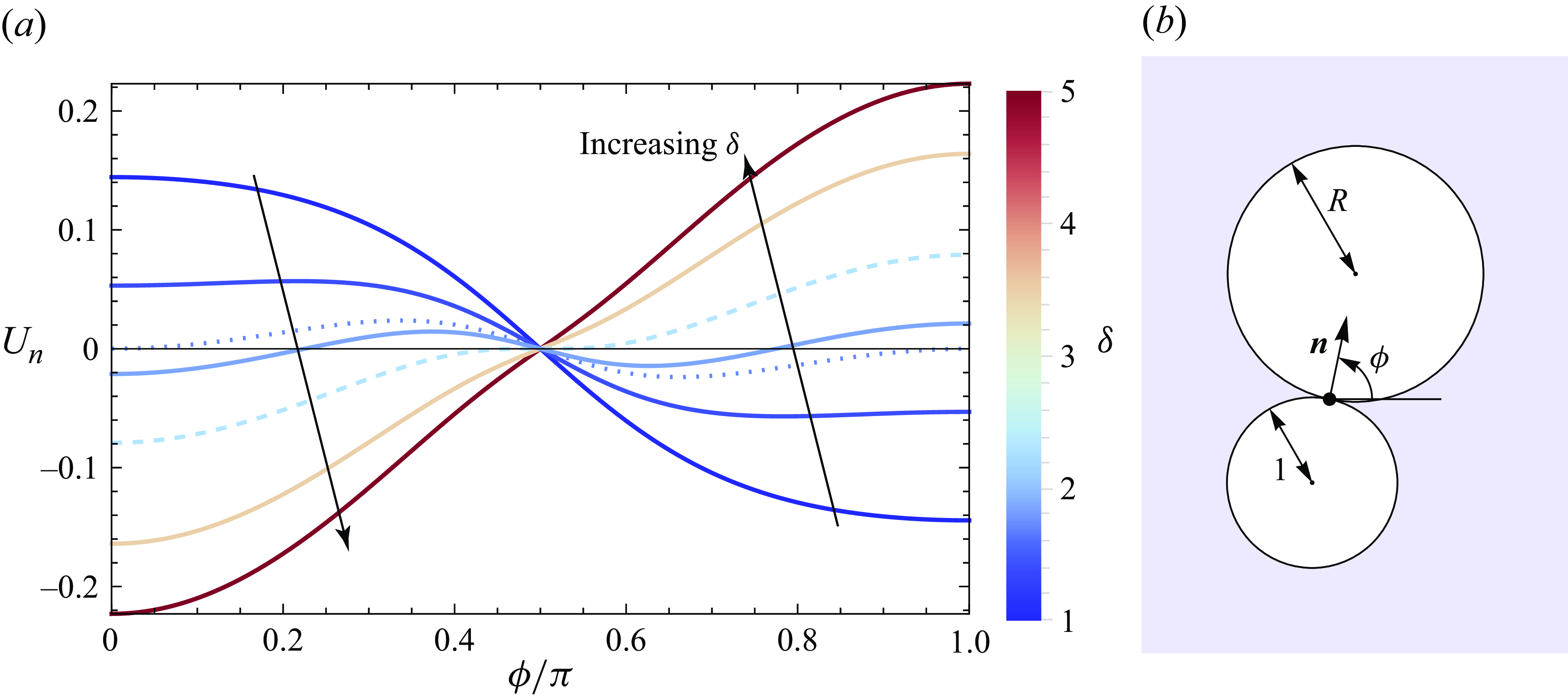
Figure 12. (a) The relative normal velocity, $U_n$
, of the two bubbles as a function of the polar angle,
$U_n$
, of the two bubbles as a function of the polar angle, $\phi$
, for a fixed
$\phi$
, for a fixed $R=2$
and
$R=2$
and $\delta$
shown by the colour bar. The dotted and dashed curves show
$\delta$
shown by the colour bar. The dotted and dashed curves show $U_n$
as a function of
$U_n$
as a function of $\phi$
at
$\phi$
at $\delta =\delta _1(2)$
, and
$\delta =\delta _1(2)$
, and $\delta =\delta _2(2)$
, respectively (see § 5.2). (b) Schematic of two bubbles touching showing the definitions of
$\delta =\delta _2(2)$
, respectively (see § 5.2). (b) Schematic of two bubbles touching showing the definitions of $\boldsymbol {n}$
and
$\boldsymbol {n}$
and $\phi$
.
$\phi$
.
6. The deformation of two bubbles
6.1. Asymptotic expansions
In this section, we calculate the first-order corrections in $\epsilon$
, the bubble aspect ratio (2.3), to the shapes of a pair of bubbles, each of which undergoes deformations induced by the presence of the other. For simplicity, we consider two bubbles aligned in the direction of the flow with centres at positions
$\epsilon$
, the bubble aspect ratio (2.3), to the shapes of a pair of bubbles, each of which undergoes deformations induced by the presence of the other. For simplicity, we consider two bubbles aligned in the direction of the flow with centres at positions $(0,0)$
and
$(0,0)$
and $(\sigma ,0)$
, respectively, in the
$(\sigma ,0)$
, respectively, in the $(x,y)$
-plane (see figure 13). At leading order, the bubbles are circles of radii
$(x,y)$
-plane (see figure 13). At leading order, the bubbles are circles of radii $ R_1=1$
, and
$ R_1=1$
, and $R_2=R$
, with velocities
$R_2=R$
, with velocities $\mathcal {U}_1=U_1$
and
$\mathcal {U}_1=U_1$
and $\mathcal {U}_2=U_2$
given by (3.16), respectively. We assume that the deformations occur faster than the time scale,
$\mathcal {U}_2=U_2$
given by (3.16), respectively. We assume that the deformations occur faster than the time scale, $1/|U_1-U_2|$
for the relative motion of the two bubbles, which means we can treat the deformations as quasi-steady, with
$1/|U_1-U_2|$
for the relative motion of the two bubbles, which means we can treat the deformations as quasi-steady, with $\sigma$
assumed to be a known constant.
$\sigma$
assumed to be a known constant.
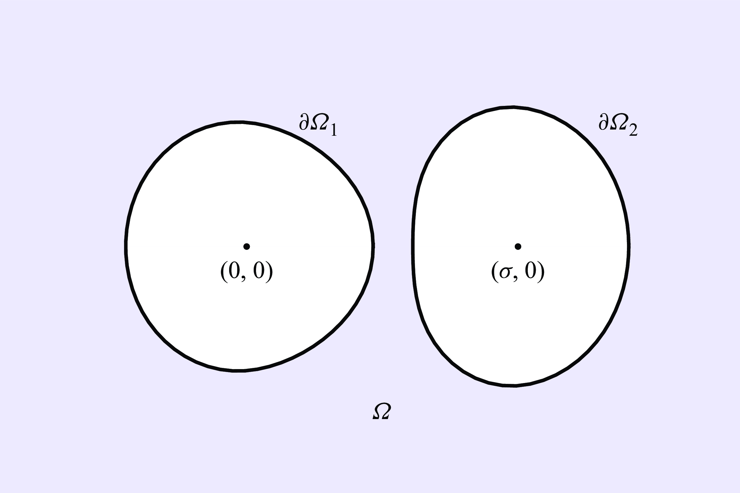
Figure 13. Schematic of the two-bubble deformation problem. The background flow is from left to right.
To find the corrections to the bubble shapes, we return to the dynamic boundary condition (2.1c
) and expand the curvatures and bubble pressures in powers of $\epsilon$
as
$\epsilon$
as
 \begin{align} &\qquad \kappa _k \sim \frac {1}{R_k}+\epsilon \kappa _{k1}+\cdots , \end{align}
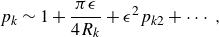 \begin{align} &p_k \sim 1+\frac {\pi \epsilon }{4R_k}+\epsilon ^2 p_{k2}+\cdots , \end{align}
for $k\in \{1,2\}$
. Note that, for completeness, one should also expand the complex potential,
$k\in \{1,2\}$
. Note that, for completeness, one should also expand the complex potential, $w(z)$
, and the bubble velocities,
$w(z)$
, and the bubble velocities, $U_1$
and
$U_1$
and $U_2$
, as asymptotic series in powers of
$U_2$
, as asymptotic series in powers of $\epsilon$
. However, to find the first-order shape correction we only need the leading-order solutions (3.9) and (3.16), and so for ease of notation we do not include an additional subscript 0 for these variables. We note that our analysis does not at present determine the first corrections to the bubble velocities due to the deformations.
$\epsilon$
. However, to find the first-order shape correction we only need the leading-order solutions (3.9) and (3.16), and so for ease of notation we do not include an additional subscript 0 for these variables. We note that our analysis does not at present determine the first corrections to the bubble velocities due to the deformations.
6.2. Deformation of the rear bubble
For the first bubble, the dynamic boundary condition (2.1c
) at $O(\epsilon ^2)$
reads
$O(\epsilon ^2)$
reads
 \begin{align} \kappa _{11} = \frac {4p_{12}}{\pi } +\frac {12\delta ^3\eta ^3}{\pi }\operatorname {Re}\left [z+W\left (\frac {1-a z}{z-a}\right )\right ] - \frac {4\delta ^2\eta ^2U_1^{2/3}}{\pi }\beta (\boldsymbol {i}\boldsymbol {\cdot }\boldsymbol {n})|\boldsymbol {i}\boldsymbol {\cdot }\boldsymbol {n}|^{2/3}, \end{align}
on $|z|=1$
. We define polar coordinates centred at
$|z|=1$
. We define polar coordinates centred at $(0,0)$
, so the bubble surface is given by
$(0,0)$
, so the bubble surface is given by $r=1+\epsilon g_1(\theta )$
, where
$r=1+\epsilon g_1(\theta )$
, where $\theta$
is the polar angle. The dynamic boundary condition (6.2) in polar coordinates is given by
$\theta$
is the polar angle. The dynamic boundary condition (6.2) in polar coordinates is given by
 \begin{align} -g_1^{\prime\prime}\! - g_1 = \frac {4p_{12}}{\pi } +\frac {12\delta ^3\eta ^3}{\pi }\operatorname {Re}\left [\mathrm {e}^{\mathrm {i}\theta }+W\!\left (\frac {1-a \mathrm {e}^{\mathrm {i}\theta }}{\mathrm {e}^{\mathrm {i}\theta }-a}\right )\!\right ] - \frac {4\delta ^2\eta ^2U_1^{2/3}}{\pi }\beta (\cos \theta )|\cos \theta |^{2/3}. \end{align}
We determine $p_{12}$
by enforcing conservation of bubble area, i.e.
$p_{12}$
by enforcing conservation of bubble area, i.e.
 \begin{align} \int _0^{2\pi }g_{1}\,\mathrm {d}\theta =-\int _0^{2\pi }\kappa _{11}\,\mathrm {d}\theta = 0. \end{align}
We solve (6.3) by expanding $g_1$
as the Fourier cosine series
$g_1$
as the Fourier cosine series
 \begin{align} g_1(\theta ) = \frac {c_0}{2}+\sum _{n=1}^{\infty } c_n \cos n \theta . \end{align}
By the area conservation condition (6.4), we find that $c_0=0$
. We further fix the centroid of the bubble at the origin, which corresponds to
$c_0=0$
. We further fix the centroid of the bubble at the origin, which corresponds to $c_1=0$
. The remaining coefficients (
$c_1=0$
. The remaining coefficients ( $n\geqslant 2)$
are determined by
$n\geqslant 2)$
are determined by
 \begin{align} c_n = \frac {1}{(n^2-1)}\int _0^{2\pi }\frac {12\delta ^3\eta ^3}{\pi ^2}\operatorname {Re}\left [W\left (\frac {1-a \mathrm {e}^{\mathrm {i}\theta }}{\mathrm {e}^{\mathrm {i}\theta }-a}\right )\right ] \cos n \theta \,\mathrm {d}\theta - \frac {4\delta ^2\eta ^2U_1^{2/3}b_n}{\pi (n^2-1)}, \end{align}
where the $b_n$
are the Fourier coefficients of
$b_n$
are the Fourier coefficients of $\beta (\cos \theta )|\cos \theta |^{2/3}$
and are given by
$\beta (\cos \theta )|\cos \theta |^{2/3}$
and are given by
 \begin{align} b_n &= \frac {\Gamma \left (\frac {5}{3}\right )\Gamma \left (\frac {n}{2}-\frac {1}{3}\right )}{4\pi 2^{2/3}\Gamma \left (\frac {n}{2}+\frac {4}{3}\right )}\left [\left ((\sqrt {3}+1)\beta _1+(\sqrt {3}-1)\beta _2\right )(-1)^{\left\lfloor \frac {n-1}{2}\right\rfloor }\right. \nonumber \\ &\quad -\left. \left ((\sqrt {3}-1)\beta _1+(\sqrt {3}+1)\beta _2\right )(-1)^{\left\lfloor \frac {n}{2}\right\rfloor }\right ]. \end{align}
Equation (6.5) then determines the first-order shape correction of the rear bubble $\partial \Omega _1$
.
$\partial \Omega _1$
.
6.3. Deformation of the front bubble
We proceed similarly with the second bubble. By defining polar coordinates centred at $(\sigma ,0)$
, we find that the bubble surface is given by
$(\sigma ,0)$
, we find that the bubble surface is given by $r=R+\epsilon g_2(\theta )$
, where
$r=R+\epsilon g_2(\theta )$
, where $g_2(\theta )$
is given by the Fourier series
$g_2(\theta )$
is given by the Fourier series
 \begin{align} g_2(\theta ) = \frac {d_0}{2}+\sum _{n=1}^{\infty } d_n \cos n \theta . \end{align}
By area conservation, we find that $d_0=0$
. We further fix the centroid of the bubble at
$d_0=0$
. We further fix the centroid of the bubble at $(\sigma ,0)$
, which corresponds to
$(\sigma ,0)$
, which corresponds to $d_1=0$
. The remaining coefficients (
$d_1=0$
. The remaining coefficients ( $n\geqslant 2)$
are determined by
$n\geqslant 2)$
are determined by
 \begin{equation} d_n = \frac {R^2}{(n^2-1)}\int _0^{2\pi }\frac {12\delta ^3\eta ^3}{\pi ^2}\operatorname {Re}\left [W\left (\frac {1-a (\sigma +R\mathrm {e}^{\mathrm {i}\theta })}{ (\sigma +R\mathrm {e}^{\mathrm {i}\theta })-a}\right )\right ] \cos n \theta \,\mathrm {d}\theta - \frac {4R^2\delta ^2\eta ^2U_1^{2/3}b_n}{\pi (n^2-1)}. \end{equation}
This then determines the first-order shape correction of the front bubble $\partial \Omega _2$
.
$\partial \Omega _2$
.
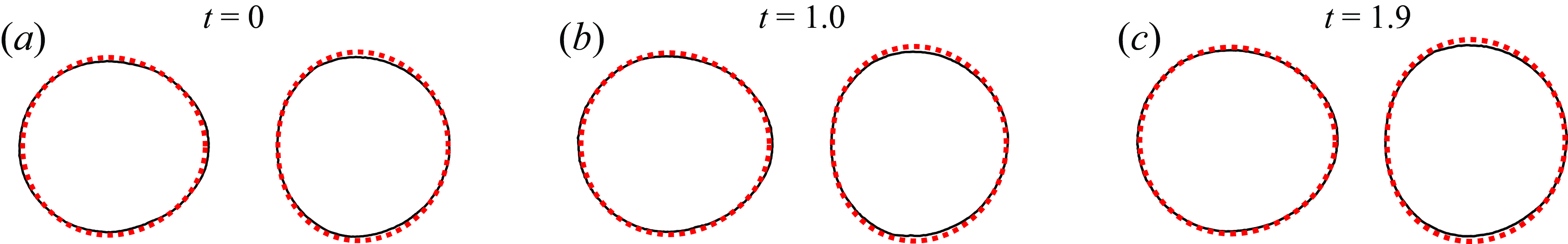
Figure 14. Experimental bubble shapes (black solid), asymptotic solution (6.5) and (6.8) (red dashed) dashed for $R=1$
,
$R=1$
, $\delta =2.86$
and
$\delta =2.86$
and $\sigma =$
(a) 2.68, (b) 2.56, (c) 2.43. The corresponding different dimensionless times
$\sigma =$
(a) 2.68, (b) 2.56, (c) 2.43. The corresponding different dimensionless times $t = \hat {t}\hat {U}/\hat {R}_1$
are shown above for the experiments. The background flow is from left to right. Experimental images have been rescaled by the rear bubble radius,
$t = \hat {t}\hat {U}/\hat {R}_1$
are shown above for the experiments. The background flow is from left to right. Experimental images have been rescaled by the rear bubble radius, $\hat {R}_1 =$
5.4 mm, for comparison with the theory. The bubble shapes from experiment and asymptotics are aligned so that the centroids of the bubble pairs coincide.
$\hat {R}_1 =$
5.4 mm, for comparison with the theory. The bubble shapes from experiment and asymptotics are aligned so that the centroids of the bubble pairs coincide.
6.4. Results
6.4.1. Identical bubbles (
$R=1$
)

In figure 14, we show example solutions for the bubble shapes at different separations, $\sigma$
, calculated using (6.5) and (6.8), with
$\sigma$
, calculated using (6.5) and (6.8), with $R=1$
,
$R=1$
, $\delta =2.86$
and
$\delta =2.86$
and $\epsilon =0.027$
, alongside experimental measurements under the same conditions. We observe good agreement between theory and experiments. The bubble in front flattens in the direction of motion (left to right), and the bubble behind elongates. In the theoretical plots, we use
$\epsilon =0.027$
, alongside experimental measurements under the same conditions. We observe good agreement between theory and experiments. The bubble in front flattens in the direction of motion (left to right), and the bubble behind elongates. In the theoretical plots, we use $\sigma$
as a proxy for time, because we assume that the deformations are quasi-steady.
$\sigma$
as a proxy for time, because we assume that the deformations are quasi-steady.

Figure 15. The in-plane bubble aspect ratios, $A_{k}$
, versus separation,
$A_{k}$
, versus separation, $\sigma$
, for the rear bubble (
$\sigma$
, for the rear bubble ( $k=1$
, dashed curve and open markers) and the front bubble (
$k=1$
, dashed curve and open markers) and the front bubble ( $k=2$
, solid curve and filled markers), with
$k=2$
, solid curve and filled markers), with $\delta =2.86$
and
$\delta =2.86$
and $\epsilon =0.027$
. The points show experimental measurements and the curves are the asymptotic predictions (6.10). The different marker shapes (triangle, circle, diamond) represent distinct pairs of bubbles that were tracked and measured as the rear bubble caught up and collided with the front bubble. The error between experiment and theory is approximately
$\epsilon =0.027$
. The points show experimental measurements and the curves are the asymptotic predictions (6.10). The different marker shapes (triangle, circle, diamond) represent distinct pairs of bubbles that were tracked and measured as the rear bubble caught up and collided with the front bubble. The error between experiment and theory is approximately $6$
%–
$6$
%– $10\,\%$
.
$10\,\%$
.
To quantify our results, we define the in-plane bubble aspect ratios as
 \begin{equation} A_k = \frac {2R_k+\epsilon (g_k(0)+g_k(\pi ))}{2R_k+2\epsilon g_k(\pi /2)}\sim 1+\frac {\epsilon }{2R_k}(g_k(0)+g_k(\pi )-2g_k(\pi /2)), \end{equation}
for $k\in \{1,2\}$
. In figure 15, we plot
$k\in \{1,2\}$
. In figure 15, we plot $A_{1,2}$
versus bubble separation,
$A_{1,2}$
versus bubble separation, $\sigma$
, for a fixed value of
$\sigma$
, for a fixed value of $\delta$
. We observe that, as the bubbles become close, the disparity between their aspect ratios increases: the bubble in front becomes more flattened, while the rear bubble develops a more pronounced elongation. There is good agreement between the predicted and experimentally measured aspect ratio
$\delta$
. We observe that, as the bubbles become close, the disparity between their aspect ratios increases: the bubble in front becomes more flattened, while the rear bubble develops a more pronounced elongation. There is good agreement between the predicted and experimentally measured aspect ratio $A_2$
of the front bubble, however, there is a constant offset of approximately
$A_2$
of the front bubble, however, there is a constant offset of approximately $0.06$
, which induces an approximate
$0.06$
, which induces an approximate
 error between the theory and experiments. The model generally over-predicts the degree of flattening of the front bubble. For the aspect ratio $A_1$
of the rear bubble, there is a discrepancy between theory and experiments. In the experiments,
$A_1$
of the rear bubble, there is a discrepancy between theory and experiments. In the experiments, $A_1$
is approximately constant, however, our model predicts this to be a monotonically decreasing function, and thus under-predicts the elongation of the rear bubble. In the experiments, the two bubbles become very close and, in this limit, we expect the theory may break down due to the three-dimensional effects in the fluid flow between the two bubbles. In addition, our dynamic boundary condition (2.1c
) is strictly valid only when the normal velocities at corresponding points on the front and rear menisci are equal and opposite; when the bubbles deform significantly this is no longer true and we should incorporate the full Burgess & Foster (Reference Burgess and Foster1990) boundary conditions on the bubble surface. Furthermore, bubbles in Hele-Shaw cells that are approaching or separating experience additional stresses due to their relative motion (Bremond, Thiam & Bibette Reference Bremond, Thiam and Bibette2008; Lai, Bremond & Stone Reference Lai, Bremond and Stone2009; Chan, Klaseboer & Manica Reference Chan, Klaseboer and Manica2010) that have not been included in our analysis.
$A_1$
is approximately constant, however, our model predicts this to be a monotonically decreasing function, and thus under-predicts the elongation of the rear bubble. In the experiments, the two bubbles become very close and, in this limit, we expect the theory may break down due to the three-dimensional effects in the fluid flow between the two bubbles. In addition, our dynamic boundary condition (2.1c
) is strictly valid only when the normal velocities at corresponding points on the front and rear menisci are equal and opposite; when the bubbles deform significantly this is no longer true and we should incorporate the full Burgess & Foster (Reference Burgess and Foster1990) boundary conditions on the bubble surface. Furthermore, bubbles in Hele-Shaw cells that are approaching or separating experience additional stresses due to their relative motion (Bremond, Thiam & Bibette Reference Bremond, Thiam and Bibette2008; Lai, Bremond & Stone Reference Lai, Bremond and Stone2009; Chan, Klaseboer & Manica Reference Chan, Klaseboer and Manica2010) that have not been included in our analysis.
In § 3 we found that, if $R=1$
, the bubbles travel at the same velocity at leading order in
$R=1$
, the bubbles travel at the same velocity at leading order in $\epsilon$
. However, in experiments, we observe that the bubbles approach each other while deforming, due to
$\epsilon$
. However, in experiments, we observe that the bubbles approach each other while deforming, due to $O(\epsilon )$
corrections to the velocities which we currently do not calculate. Ultimately, the bubbles collide and coalesce when
$O(\epsilon )$
corrections to the velocities which we currently do not calculate. Ultimately, the bubbles collide and coalesce when $\sigma \lt 1+R$
, a range that is inaccessible with our current analytical methods.
$\sigma \lt 1+R$
, a range that is inaccessible with our current analytical methods.
Wu et al. (Reference Wu, Booth, Griffiths, Howell, Nunes and Stone2024) found that, if an isolated bubble is flattened in the direction of motion, then the leading-order solution over-predicts the bubble velocity, and vice versa if the bubble is elongated. The same line of reasoning here would suggest that the velocity of the bubble at the front is over-predicted by (3.16), while the velocity of the bubble behind is under-predicted by (3.16). Thus, the bubble behind would travel faster than the bubble in front, resulting in the collision of bubbles of equal size. Similar behaviour has been observed experimentally and computationally for a pair of unconfined bubbles rising at low Reynolds numbers due to buoyancy (Manga & Stone Reference Manga and Stone1993, Reference Manga and Stone1995). As a result of the interaction between the bubbles, the leading bubble flattens in the direction of motion while the bubble behind elongates, and the distance between them decreases until they collide. Our results establish that there is an analogous mechanism for bubble collision in Hele-Shaw cells.

Figure 16. Experimental bubble shapes (black solid), asymptotic solution (6.5) and (6.8) (red dashed) for (a–c) $R=1.23$
,
$R=1.23$
, $\delta =2.55$
and
$\delta =2.55$
and $\sigma =$
(a) 2.39, (b) 2.34, (c) 2.28, (d–f)
$\sigma =$
(a) 2.39, (b) 2.34, (c) 2.28, (d–f) $R=1.65$
,
$R=1.65$
, $\delta =1.94$
and
$\delta =1.94$
and $\sigma =$
(d) 3.45, (e) 3.23, (f) 2.94. The corresponding different dimensionless times
$\sigma =$
(d) 3.45, (e) 3.23, (f) 2.94. The corresponding different dimensionless times $t = \hat {t}\hat {U}/\hat {R}_1$
are shown above for the experiments. The background flow is from left to right. Experimental images have been rescaled by the rear bubble radii,
$t = \hat {t}\hat {U}/\hat {R}_1$
are shown above for the experiments. The background flow is from left to right. Experimental images have been rescaled by the rear bubble radii, $\hat {R}_1 =$
(a–c) 2.9 mm and (d–f) 4.8 mm, for comparison with the theory. The bubble shapes from experiment and asymptotics are aligned so that the centroids of the bubble pairs coincide.
$\hat {R}_1 =$
(a–c) 2.9 mm and (d–f) 4.8 mm, for comparison with the theory. The bubble shapes from experiment and asymptotics are aligned so that the centroids of the bubble pairs coincide.
6.4.2. Bubbles of different radii (
$R \neq 1$
)

In the absence of shape deformation, larger bubbles are expected to travel faster than smaller ones (Booth et al. Reference Booth, Griffiths and Howell2023). For this case, conditions were derived in § 5.2 under which a larger bubble can catch and collide with a smaller bubble in finite time. In § 6.4.1, we presented suggestions of a further mechanism arising from shape deformation by which two bubbles of equal size can collide. Here, we show that shape deformations and the resulting effects on the surrounding flow can be strong enough to enable a smaller bubble to catch a larger bubble.
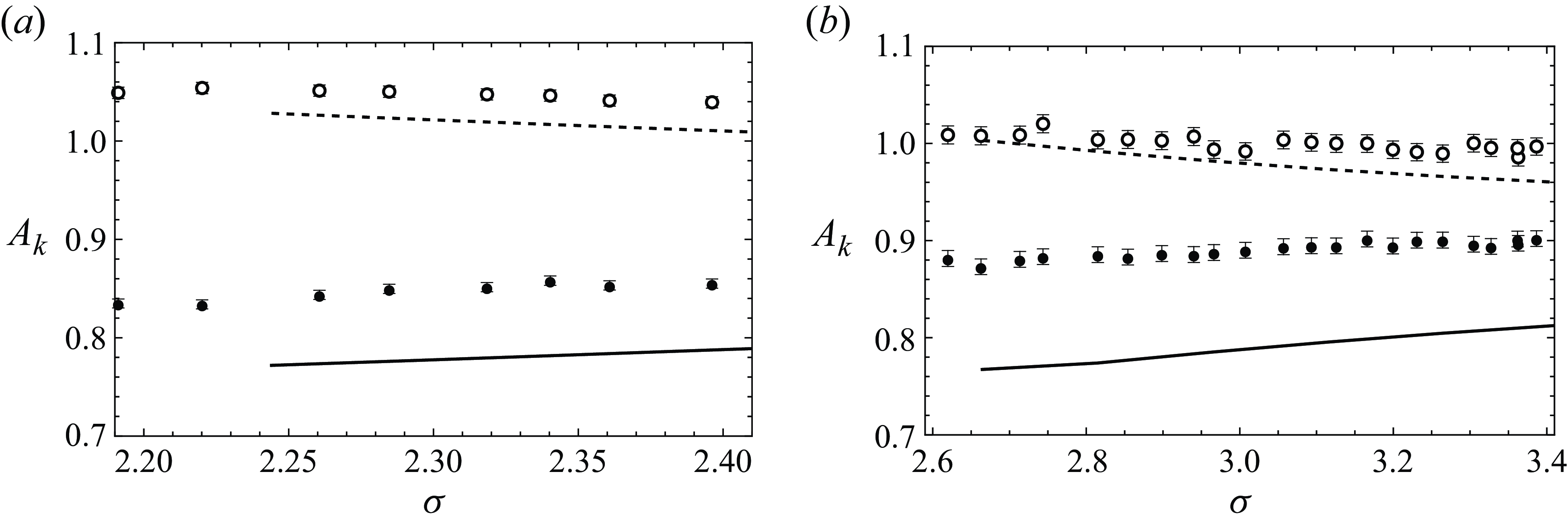
Figure 17. The bubble aspect ratios, $A_{k}$
, versus separation,
$A_{k}$
, versus separation, $\sigma$
, for the rear bubble (
$\sigma$
, for the rear bubble ( $k=1$
, dashed curve and open markers) and the front bubble (
$k=1$
, dashed curve and open markers) and the front bubble ( $k=2$
, solid curve and filled markers), with (a)
$k=2$
, solid curve and filled markers), with (a) $R=1.23$
,
$R=1.23$
, $\delta =2.55$
and
$\delta =2.55$
and $\epsilon =0.03$
(b),
$\epsilon =0.03$
(b), $R=1.65$
,
$R=1.65$
, $\delta =1.94$
and
$\delta =1.94$
and $\epsilon =0.05$
. The points show experimental measurements, and the curves are the asymptotic predictions (6.10). The error between experiment and theory is approximately (a)
$\epsilon =0.05$
. The points show experimental measurements, and the curves are the asymptotic predictions (6.10). The error between experiment and theory is approximately (a) $5$
%–
$5$
%– $7\,\%$
and (b)
$7\,\%$
and (b) $10$
%–
$10$
%– $13\,\%$
.
$13\,\%$
.
We show example solutions for the bubble shapes given by (6.5) and (6.8) alongside experimental images with, $R=1.23$
and
$R=1.23$
and $\delta =2.55$
in figures 16(a)–16(c) and
$\delta =2.55$
in figures 16(a)–16(c) and $R=1.65$
and
$R=1.65$
and $\delta =1.94$
in figures 16(d)–16(f). Similarly to the examples of the bubbles with the same leading-order radius (see figure 14), the leading bubble flattens in the direction of motion, whereas the rear bubble elongates. To quantify this observation, we plot the bubble aspect ratios
$\delta =1.94$
in figures 16(d)–16(f). Similarly to the examples of the bubbles with the same leading-order radius (see figure 14), the leading bubble flattens in the direction of motion, whereas the rear bubble elongates. To quantify this observation, we plot the bubble aspect ratios $A_{1,2}$
versus separation,
$A_{1,2}$
versus separation, $\sigma$
, in figure 17. We observe good agreement between theory and experiments. In particular, we correctly predict that
$\sigma$
, in figure 17. We observe good agreement between theory and experiments. In particular, we correctly predict that $A_1\gt A_2$
. Again, there is a discrepancy between the experimentally measured aspect ratios and theoretical predictions, which we attribute to the same reasons as discussed in § 6.4.1. Nevertheless, these results hint that, although the smaller rear bubble is expected to lag behind the larger front bubble when they are both circular, deformations may allow for a region of parameter space in which a smaller bubble can catch up to a larger one. Several collisions of this type have been observed experimentally, and the progression of shape deformation for a few examples is shown in figure 16. To establish this result theoretically, one would need to find the perturbation to the bubble speeds, for example by performing a complex variable analysis similar to that done by Wu et al. (Reference Wu, Booth, Griffiths, Howell, Nunes and Stone2024). We leave such analysis for future work.
$A_1\gt A_2$
. Again, there is a discrepancy between the experimentally measured aspect ratios and theoretical predictions, which we attribute to the same reasons as discussed in § 6.4.1. Nevertheless, these results hint that, although the smaller rear bubble is expected to lag behind the larger front bubble when they are both circular, deformations may allow for a region of parameter space in which a smaller bubble can catch up to a larger one. Several collisions of this type have been observed experimentally, and the progression of shape deformation for a few examples is shown in figure 16. To establish this result theoretically, one would need to find the perturbation to the bubble speeds, for example by performing a complex variable analysis similar to that done by Wu et al. (Reference Wu, Booth, Griffiths, Howell, Nunes and Stone2024). We leave such analysis for future work.
7. Conclusions
In this paper we analyse a model and present new experimental results for the motion of two bubbles in a Hele-Shaw cell. The mathematical model depends on two dimensionless parameters, the bubble aspect ratio $\epsilon$
and the capillary number
$\epsilon$
and the capillary number $\mathrm {Ca}$
, both of which are assumed to be small. Specifically, we consider the asymptotic distinguished limit in which
$\mathrm {Ca}$
, both of which are assumed to be small. Specifically, we consider the asymptotic distinguished limit in which $\mathrm {Ca}=O (\epsilon ^3 )$
and the bubbles are circular to leading order. Through the use of complex variable methods, we derive analytical equations of motion for the two bubbles. In general, the instantaneous bubble velocities are obtained by solving the system of nonlinear algebraic equations (3.16).
$\mathrm {Ca}=O (\epsilon ^3 )$
and the bubbles are circular to leading order. Through the use of complex variable methods, we derive analytical equations of motion for the two bubbles. In general, the instantaneous bubble velocities are obtained by solving the system of nonlinear algebraic equations (3.16).
For two non-identical bubbles such that the larger bubble is initially far behind the smaller bubble with a small transverse offset, there are two possible outcomes. The first is that the bubbles collide, while in the second, due to the nonlinear interactions, instead of colliding they rotate around each other. Which behaviour occurs depends on the value of the Bretherton parameter $\delta$
. For each bubble radius ratio,
$\delta$
. For each bubble radius ratio, $R$
, there exists a first critical Bretherton parameter,
$R$
, there exists a first critical Bretherton parameter, $\delta _1(R)$
, above which it is impossible for two aligned bubbles to collide. Then there exists a second critical Bretherton parameter,
$\delta _1(R)$
, above which it is impossible for two aligned bubbles to collide. Then there exists a second critical Bretherton parameter, $\delta _2(R)$
, above which any trajectory in which the bubbles are initially far apart in the
$\delta _2(R)$
, above which any trajectory in which the bubbles are initially far apart in the $x$
-direction results in the bubbles rotating around one another, and if the bubbles are initially close with the larger bubble behind, the bubbles will rotate around one another and then collide with the large one in front. We find that if
$x$
-direction results in the bubbles rotating around one another, and if the bubbles are initially close with the larger bubble behind, the bubbles will rotate around one another and then collide with the large one in front. We find that if $\delta \geqslant \delta ^*\approx 3.10$
then the bubbles must always rotate around one another regardless of their radii if the smaller bubble is initially in front. Furthermore, we establish that, if the bubbles collide, they do so in finite time.
$\delta \geqslant \delta ^*\approx 3.10$
then the bubbles must always rotate around one another regardless of their radii if the smaller bubble is initially in front. Furthermore, we establish that, if the bubbles collide, they do so in finite time.
Finally, we find the leading-order perturbations to the bubble shapes for a pair of bubbles in a Hele-Shaw cell aligned with a uniform background flow. If the bubbles are the same size, we observe that the bubble in front flattens in the direction of motion, while the bubble behind elongates. By analogy with the results for an isolated bubble obtained by Wu et al. (Reference Wu, Booth, Griffiths, Howell, Nunes and Stone2024), we argue that these deformations permit the bubble behind to catch and collide with the bubble in front, despite the leading-order solution predicting that two identical bubbles should travel at the same velocity. Furthermore, this same pattern of deformation is seen in systems of two bubbles with a larger bubble in front, suggesting that we could see a smaller bubble catch a larger one. Such collisions are indeed observed in experiments. It is the subject of future work to calculate the perturbations to the bubble velocities and thus confirm these observations theoretically.
As one possible application, the work presented in this paper provides a foundation for studying the interactions among suspensions of bubbles in microfluidic configurations. As is common in the study of suspensions, the analytical results obtained here for the motion of two bubbles can be used to derive an approximate pairwise interaction model. Such a model will accurately capture situations in which two bubbles become close, where the commonly used dipole model (Beatus et al. Reference Beatus, Tlusty and Bar-Ziv2006, Reference Beatus, Bar-Ziv and Tlusty2012; Green Reference Green2018) breaks down.
Supplementary movies
Supplementary movies are available at https://doi.org/:10.1017/jfm.2025.322.
Funding
D.J.B. is grateful to EPSRC, grant reference number EP/V520202/1, for funding. K.W. gratefully acknowledges the support of the National Science Foundation Graduate Research Fellowship under Grant No. DGE-2039656.
Declaration of interests
The authors report no conflict of interest.
Appendix A. Small separation asymptotics and computation of
$\boldsymbol{\delta}$
1 and
$\boldsymbol{\delta}$
2


A.1. Small separation asymptotic expansions
In § 5.2, we find two conditions, one necessary and one sufficient, for the dividing trajectory to completely enclose circle $\sigma =1+R$
and thus prevent collision between two initially separated bubbles. For each condition we find a value of
$\sigma =1+R$
and thus prevent collision between two initially separated bubbles. For each condition we find a value of $\delta = \delta _k$
, for
$\delta = \delta _k$
, for $k\in \{1,2\}$
, at which condition
$k\in \{1,2\}$
, at which condition $k$
is first satisfied (see § 5.2). We will show how to calculate the values of
$k$
is first satisfied (see § 5.2). We will show how to calculate the values of $\delta _1$
and
$\delta _1$
and $\delta _2$
in the sections below.
$\delta _2$
in the sections below.
First, we calculate the behaviour of the functions $f_k$
defined by (3.14) in the limit
$f_k$
defined by (3.14) in the limit $\sigma \rightarrow 1+R$
, namely
$\sigma \rightarrow 1+R$
, namely
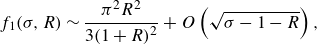 \begin{align} &\qquad\quad f_1(\sigma ,R) \sim \frac {\pi ^2 R^2}{3(1+R)^2} +O\left (\sqrt {\sigma -1-R}\right ), \end{align}
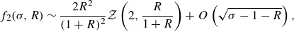 \begin{align} &f_2(\sigma ,R)\sim \frac {2R^2}{(1+R)^2} \mathcal {Z}\left (2,\frac {R}{1+R}\right )+O\left (\sqrt {\sigma -1-R}\right ), \end{align}
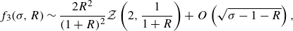 \begin{align} &f_3(\sigma ,R) \sim \frac {2R^2}{(1+R)^2} \mathcal {Z}\left (2,\frac {1}{1+R}\right ) +O\left (\sqrt {\sigma -1-R}\right ), \end{align}
where $\mathcal {Z}(s,b)$
is the Hurwitz zeta function (Kanemitsu, Katsurada & Yoshimoto Reference Kanemitsu, Katsurada and Yoshimoto2000) given by
$\mathcal {Z}(s,b)$
is the Hurwitz zeta function (Kanemitsu, Katsurada & Yoshimoto Reference Kanemitsu, Katsurada and Yoshimoto2000) given by
 \begin{align} \mathcal {Z}(s,b) = \sum _{n=0}^{\infty } \frac {1}{(n+b)^s}. \end{align}
A.2. Computation of
$\delta _1$

To find the value of $\delta _1$
at which the stationary points exist on the surface
$\delta _1$
at which the stationary points exist on the surface $|z_1-z_2|=1+R$
, we use the behaviour of
$|z_1-z_2|=1+R$
, we use the behaviour of $f_k$
(A1) in the limit
$f_k$
(A1) in the limit $\sigma \rightarrow 1+R$
to obtain the system
$\sigma \rightarrow 1+R$
to obtain the system
 \begin{align} \frac {2R^2}{(1+R)^2}\left (\frac {\pi ^2}{6} - \mathcal {Z}\left (2,\frac {R}{1+R}\right )\right )(U-1)&= -U +\frac {U^{2/3}}{\delta _1}, \end{align}
 \begin{align} \frac {2R}{(1+R)^2}\left (\frac {\pi ^2}{6} - \mathcal {Z}\left (2,\frac {1}{1+R}\right )\right )(U-1)&= -RU +\frac {U^{2/3}}{\delta _1}. \end{align}
We can easily eliminate $\delta _1$
from the (A3) by subtracting the two equations, which leaves a linear equation for
$\delta _1$
from the (A3) by subtracting the two equations, which leaves a linear equation for $U$
. The solution for
$U$
. The solution for $U$
is then substituted back into one of the equations to obtain an explicit (though unpleasant) formula for
$U$
is then substituted back into one of the equations to obtain an explicit (though unpleasant) formula for $\delta _1(R)$
.
$\delta _1(R)$
.
We observe that $\delta _1$
tends to a finite constant as
$\delta _1$
tends to a finite constant as $R\rightarrow 1^+$
. To find the value of this constant we have to be careful because the equations have a one-parameter family of solutions when
$R\rightarrow 1^+$
. To find the value of this constant we have to be careful because the equations have a one-parameter family of solutions when $R=1$
, as the bubbles travel at the same velocity. To find the limiting value we let
$R=1$
, as the bubbles travel at the same velocity. To find the limiting value we let $R=1+\varepsilon$
, where
$R=1+\varepsilon$
, where $0\lt \varepsilon \ll 1$
, and expand
$0\lt \varepsilon \ll 1$
, and expand $U\sim U^{(0)} +\varepsilon U^{(1)} +\cdots$
and
$U\sim U^{(0)} +\varepsilon U^{(1)} +\cdots$
and $\delta _1 \sim \delta _1^{(0)}+\varepsilon \delta _1^{(1)}+\cdots$
. At
$\delta _1 \sim \delta _1^{(0)}+\varepsilon \delta _1^{(1)}+\cdots$
. At $O(1)$
both equations in (A3) give
$O(1)$
both equations in (A3) give
 \begin{align} \frac {\pi ^2}{6}\left (1-U^{(0)}\right ) = -U^{(0)}+\frac {\left (U^{(0)}\right )^{2/3}}{\delta _1^{(0)}}, \end{align}
which gives us a one-parameter family of solutions. To find the relevant solution, we need to use a solvability condition. To that end we subtract (A3b
) from (A3a
) and divide by $R-1$
before expanding as above to obtain
$R-1$
before expanding as above to obtain
 \begin{align} \frac {7}{2}\mathcal {Z}(3)\left (1-U^{(0)}\right )+2U^{(0)}=\frac {\left (U^{(0)}\right )^{2/3}}{\delta _1^{(0)}}, \end{align}
where $\mathcal {Z}(s)=\mathcal {Z}(s,1)$
is the Riemann zeta function. Solving (A4) and (A5) simultaneously gives
$\mathcal {Z}(s)=\mathcal {Z}(s,1)$
is the Riemann zeta function. Solving (A4) and (A5) simultaneously gives
 \begin{align} U^{(0)}&=1+\frac {6}{21 \mathcal {Z} (3)-\pi ^2-6}\approx 1.64, & \delta _1^{(0)}&=\frac {\left (U^{(0)}\right )^{2/3}}{U^{(0)}+\pi ^2/6\left (1-U^{(0)}\right )} \approx 2.37. \end{align}
In the other extreme as $R\rightarrow \infty$
, as suggested by figure 10, it may be shown that
$R\rightarrow \infty$
, as suggested by figure 10, it may be shown that $\delta _1(R)$
tends to a finite positive limit, namely
$\delta _1(R)$
tends to a finite positive limit, namely $2^{-1/3}\approx 0.79$
.
$2^{-1/3}\approx 0.79$
.
A.3. Computation of
$\delta _2$

To find the value of $\delta _2$
, we need to determine when
$\delta _2$
, we need to determine when $\partial U_n/\partial \phi = 0$
at
$\partial U_n/\partial \phi = 0$
at $\sigma =1+R$
,
$\sigma =1+R$
, $\phi =\pi /2$
, which can be written as
$\phi =\pi /2$
, which can be written as
 \begin{align} \frac {\partial V_1}{\partial \phi }-\frac {\partial V_2}{\partial \phi } +U_2-U_1 =0. \end{align}
From (3.16) we obtain
 \begin{align} \quad\frac {2R^2}{(1+R)^2}\left (\frac {\pi ^2}{6}(U_2-1)+\mathcal {Z}\left (2,\frac {R}{1+R}\right )(U_1-1)\right ) &= U_1-\frac {U_1^{2/3}}{\delta _2}, \end{align}
 \begin{align} \frac {2R^2}{(1+R)^2}\left (\frac {\pi ^2}{6}(U_1-1)+\mathcal {Z}\left (2,\frac {1}{1+R}\right )(U_2-1)\right ) &= R^2U_2-\frac {RU_2^{2/3}}{\delta _2}, \\[6pt] \nonumber \end{align}
at $(\sigma ,\phi )=(1+R,\pi /2)$
. By differentiating (3.16) with respect to
$(\sigma ,\phi )=(1+R,\pi /2)$
. By differentiating (3.16) with respect to $\phi$
and taking the imaginary part we obtain
$\phi$
and taking the imaginary part we obtain
 \begin{align} \frac {2R^2}{(1+R)^2}\left (\frac {\pi ^2}{6}\left (\frac {\partial V_2}{\partial \phi }-2(U_2-1)\right )-\mathcal {Z}\left (2,\frac {R}{1+R}\right )\frac {\partial V_1}{\partial \phi }\right )&= -\frac {\partial V_1}{\partial \phi }\left (1-\frac {1}{\delta _2 U_1^{1/3}}\right ), \end{align}
 \begin{align} \frac {2R^2}{(1+R)^2}\left (\frac {\pi ^2}{6}\left (\frac {\partial V_1}{\partial \phi }-2(U_1-1)\right )-\mathcal {Z}\left (2,\frac {1}{1+R}\right )\frac {\partial V_2}{\partial \phi }\right )&= -\frac {\partial V_2}{\partial \phi }\left (R^2-\frac {R}{\delta _2 U_2^{1/3}}\right ). \end{align}
These equations (A7) form a closed system of five nonlinear equations for five unknowns $\{\delta _2,U_1,U_2,\partial V_1/\partial \phi ,\partial V_2/\partial \phi \}$
, which can be solved numerically via, for example, Newton’s method.
$\{\delta _2,U_1,U_2,\partial V_1/\partial \phi ,\partial V_2/\partial \phi \}$
, which can be solved numerically via, for example, Newton’s method.


 Open access