


Introduction
The analysis of multi-environment trial (MET) data is a fundamental and recurring task for the selection of superior varieties in a plant breeding programme. Smith et al. (Reference Smith, Cullis and Thompson2005) provided a comprehensive review of statistical methods for MET data and this still covers the most popular methods currently used. The methods can be broadly classified into linear mixed model (LMM) and biplot analyses. LMMs are a widely used class of statistical models that include both fixed and random effects and accommodate a range of variance structures to allow for heterogeneity and correlation. Early applications for MET data include Patterson et al. (Reference Patterson, Silvey, Talbot and Weatherup1977) and Patterson and Silvey (Reference Patterson and Silvey1980), who used LMMs that included main effects for varieties and environments, and variety by environment interaction (VEI) effects. The variance structures for random effects had simple component forms, commensurate with the assumption of independent effects with homogeneous variance. Since the late 1990s, several research groups have developed and recommended LMM that incorporate factor analytic (FA) structures for the variety effects in different environments. This allows for a very general pattern of genetic variance and covariance heterogeneity. Henceforth, this model will be referred to as a factor analytic linear mixed model (FALMM). Key papers authored by advocates of these models include Gogel et al. (Reference Gogel, Cullis and Verbyla1995), Piepho (Reference Piepho1997, Reference Piepho1998a), Smith et al. (Reference Smith, Cullis and Thompson2001, Reference Smith, Norman, Kuchel and Cullis2021b), Burgueno et al. (Reference Burgueno, Crossa, Cotes, San Vicente and Das2011) and Meyer (Reference Meyer2009). Biplot approaches involve the application of a singular value decomposition to a two-way table indexed by varieties and environments, followed by a biplot graphical representation of the first two principal components. This approach was popularised for MET data under the banner of Additive Main effects and Multiplicative Interaction models (Gauch, Reference Gauch1992) and the most common current method of this type is the GGE-biplot method (see, for example, Yan and Kang, Reference Yan and Kang2002 and Yan et al., Reference Yan, Nilsen and Beattie2023).
The analysis process for METs should be no different from any other data analysis in that it should consist of two main activities. Lee et al. (Reference Lee, Nelder and Pawitan2006) discuss this in detail and reference Lane and Nelder (Reference Lane and Nelder1982) when they state that ‘the first (activity) is model selection, which aims to find parsimonious well-fitting models for the basic responses being measured, and the second is model prediction, where the output from the primary analysis is used to derive summarising quantities of interest together with their uncertainties’. It is well known that for the purposes of variety selection, a ‘well-fitting’ MET model must accommodate a range of sources of variation associated with both genetic and non-genetic effects and field plot errors. It is crucial that the model appropriately accommodates VEI and that it allows inclusion of information on the genetic relatedness of varieties, either via ancestral or genomic data (Oakey et al., Reference Oakey, Verbyla, Pitchford, Cullis and Kuchel2006, Reference Oakey, Verbyla, Cullis, Wei and Pitchford2007). Non-genetic effects associated with experimental designs should be included, and the model should allow for error variance heterogeneity between environments and spatial correlation within environments. Accommodating all of these sources appropriately in the model will improve the accuracy of ‘output from the primary analysis’. The FALMM, in particular the model proposed by Smith et al. (Reference Smith, Cullis and Thompson2001) and extended for genetic relatedness by Oakey et al. (Reference Oakey, Verbyla, Cullis, Wei and Pitchford2007), successfully achieves this aim. This is, therefore, the model used in the current paper.
The output from the primary analysis must be summarised in a manner that facilitates variety selection. In the presence of VEI, in particular crossover VEI which is synonymous with changes in variety rankings, it makes no sense to base selection on the standard concept of variety main effects or some analogous measure of overall performance across all environments in the MET. Instead, variety performance needs to be summarised for ‘meaningful’ groups of environments. Within the framework of a FALMM, Smith et al. (Reference Smith, Norman, Kuchel and Cullis2021b) addressed this using the fundamental parameters in the FA model, namely the factor loadings, to form groups of environments. Given that the factor loadings represent the latent environmental covariates that are driving the VEI, these groups discriminate varieties with differential responses and thence differential patterns of VEI. They are therefore called interaction classes (iClasses). Smith et al. (Reference Smith, Norman, Kuchel and Cullis2021b) defined overall variety performance for each iClass by averaging variety predictions across the associated environments. This facilitates selection of the best varieties within each iClass so addresses the ‘what wins where’ question, which has become a widely used catchphrase in the biplot literature. This question should be extended to include ‘… and by how much’ as it is important to have a prediction of variety differences on the scale of the trait under consideration, together with a measure of uncertainty. This is an integral part of iClass overall performance which is reported in the units of measurement (for example, t/ha for grain yield).
Smith et al. (Reference Smith, Norman, Kuchel and Cullis2021b) developed the concept of iClasses within the framework of FALMMs in which the genetic effects for different varieties were assumed independent. They did this for ease of demonstration but stressed that, in general, the analysis of plant breeding METs will benefit greatly from the inclusion of information on the genetic relatedness of varieties. This can be achieved with the use of a relationship matrix which may be based on ancestral (pedigree) or genomic (marker) information. In the case of in-bred crops, the genetic effects in the FALMM are partitioned into additive (with a variance structure that involves the relationship matrix) and non-additive effects. As commented by Oakey et al. (Reference Oakey, Verbyla, Pitchford, Cullis and Kuchel2006), such a partitioning means that ‘a single analysis will allow both the selection of potential parents for future breeding programmes using additive effects and promising commercial lines combining both additive and non-additive effects, i.e. the overall or total genetic effect’. The FALMM with both additive and non-additive genetic effects involves two separate FA models, one for each set of effects (see Oakey et al., Reference Oakey, Verbyla, Cullis, Wei and Pitchford2007; Beeck et al., Reference Beeck, Cowling, Smith and Cullis2010; Smith and Cullis, Reference Smith and Cullis2018; Tolhurst et al., Reference Tolhurst, Mathews, Smith and Cullis2019). iClass methodology that can be applied in this setting is the focus of the current paper. Parental selection involves a straightforward application of the concepts in Smith et al. (Reference Smith, Norman, Kuchel and Cullis2021b) to the FA model for the additive effects alone, whereas the selection of varieties based on total (additive plus non-additive) effects requires an extension that incorporates both the additive and non-additive FA models.
Many authors have noted that, in addition to knowing ‘what wins where’, it is also important to characterise the stability of variety performance across environments. A seminal review paper is that of Lin et al. Reference Lin, Binns and Leftkovitch1986, who noted that ‘the concept of stability is by no means unambiguous’. They provided a helpful table that summarised nine commonly used measures and highlighted the differences in interpretations. Many of these methods are popular today, the most widely used being associated with regressions of the observed data for a variety of an environmental index defined using the mean of all observations for the environment. Key references for this type of measure are Finlay and Wilkinson (1963), Eberhart and Russell (1966) and Digby (Reference Digby1979). Oman (Reference Oman1991), Gogel et al. (Reference Gogel, Cullis and Verbyla1995) and Piepho (Reference Piepho1997) considered mixed model versions of this approach. Piepho (Reference Piepho1998b) provided a comprehensive review of stability measures (including those in Lin et al. Reference Lin, Binns and Leftkovitch1986) and showed how each relates to an underlying statistical model. He made a pivotal point, namely that ‘Usefulness of any measure of stability depends crucially on how well the underlying model approximates the real data’. Of the commonly used stability measures, arguably the best fitting model is the regression on the environmental mean model. However, it is well known that this rarely provides a ‘good approximation to the data’ since it typically only explains a very small proportion of VEI. In contrast, the FALMM routinely provides a good fit for MET data so is a prudent choice of model on which to build a stability measure. Based on this model, Smith and Cullis (Reference Smith and Cullis2018) proposed a stability measure that has a similar flavour to the regression approaches but involves the latent regression implicit in an FA model. Specifically, for each variety, the stability measure is the root mean square deviation of the predicted effects from the fitted values for the latent regression associated with the first (most important) factor. The assumption is that the estimated loadings for the first factor are all positive so it represents the scale (non-crossover) component of VEI, and hence, the deviations reflect crossover VEI. This measure is sub-optimal, however, in the sense that it restricts attention to the first factor only, so ignores the latent regressions on the higher-order factors which typically account for a non-ignorable amount of VEI. In the current paper, therefore, a stability measure is proposed that captures the VEI associated with all the factors in the FALMM (or as many as the breeder wishes to use) and has no requirement about positive signs for the estimated loadings in the first factor. The measure can be visualised in the interaction plots of Smith et al. (Reference Smith, Norman, Kuchel and Cullis2021b) which depict the overall performance of a small user-defined set of varieties across iClasses. Due to the manner in which iClasses are formed, there is a natural ordering on this plot, with the major sources of VEI being contrasted across iClasses on opposite sides of the plot. This allows a visual inspection of VEI, or equivalently, stability of performance across iClasses, for the nominated varieties. Stability is therefore indicated by the relative magnitude of the peaks and troughs across the interaction plot. In the current paper, a numerical measure that quantifies this form of stability is developed. It is easily computed in conjunction with iClass overall performance for all varieties in the MET dataset. As such it may be useful as an additional trait for selection.
The main goals of this paper are to extend the iClass methodology introduced in Smith et al. (Reference Smith, Norman, Kuchel and Cullis2021b) for analyses that include information on the genetic relatedness of varieties and to present a new measure of stability of variety performance. The utility of the methods is demonstrated using a motivating example from an Australian lentil breeding programme.
Materials and methods
The motivating example considered in this paper was provided by the Agriculture Victoria lentil breeding programme. This programme involves five stages of variety testing, labelled as L0, L1, L2, L3 and L4. Using the techniques of Smith et al. (Reference Smith, Ganesalingam, Lisle, Kadkol, Hobson and Cullis2021a), a dataset was constructed to facilitate selections for stages L0, L1, L2 and L3 in 2023. In this paper, the analysis is conducted for this entire dataset, but in the interests of brevity, the iClass methodology is applied for one set of selections only. The L3 selections have been chosen for this purpose, partly because these comprise the smallest number of varieties so the methodology is most easily demonstrated and partly because these are the final decisions prior to commercial release so have immediate ramifications for both the breeding programme and growers.
Overall, the dataset contains 160 trials grown in 90 environments and a total of 10 356 unique varieties. In this paper a ‘trial’ refers to the physical collection of field plots onto which a valid experimental design is imposed. An ‘environment’ is defined by the geographic location and year of planting of a trial. Of the 90 environments in the MET dataset, 43 encompassed multiple trials due to the presence of trials for different stages at the same location. All trials in an environment were managed in the same way and had the same plot dimensions. The number of varieties per trial ranged from 36 to 2487 and the number of plots from 108 to 3024. In 70 trials, partially replicated designs (Cullis et al., Reference Cullis, Smith, Cocks and Butler2020) were employed in which some varieties were tested without replication (that is, a single plot for each) and others were tested using two replicate plots. In the remaining trials, there was near complete replication with either two or three replicates of most varieties.
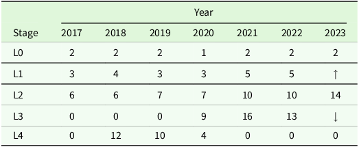
The distribution of trials across stages and years is shown in Table 1. Note that, prior to 2023, varieties in different stages of testing were grown in separate trials, whereas in 2023, varieties from stages L1, L2 and L3 were grown together in the same trial. The inclusion of the L4 trials from 2018, 2019 and 2020 warrants discussion. These were included in accordance with one of the key philosophies of Smith et al. (Reference Smith, Ganesalingam, Lisle, Kadkol, Hobson and Cullis2021a), namely to maximise the amount of observed data for the varieties under consideration for selection. The varieties impacted by the inclusion of the L4 trials were five 2023 L3 varieties under consideration for commercial release. Inclusion of the L4 trials provided an additional two years of data for each of these varieties and between 22 and 26 additional environments. It is acknowledged that the inclusion of these trials, some of which were the smallest in the dataset with only 36 varieties, must be investigated in terms of any potential negative impact on the estimation of genetic variance parameters. This is fully explored in the Supplementary Material, Section 1, where it is shown that the impact is likely to be negligible, with any associated losses in the reliability of variety predictions being far outweighed by the benefits of including the additional data. Supplementary Material, Section 1 demonstrates the statistical benefits of including the L4 trials. It should also be noted there are substantial benefits in terms of grower confidence, since, in general, L4 trials are grown in more locations than earlier stage trials and the inclusion of the L4 trials in the current dataset provided an additional 14 location/year combinations (environments) for variety comparisons.
Table 1. Multi-environment trial dataset for L0, L1, L2 and L3 stage selection decisions in 2023: number of trials included from each stage and year. Note that, prior to 2023, the entries in different stages were grown in separate trials, whereas in 2023, the L1, L2 and L3 entries were grown together in the same trial
In the current paper, genetic relatedness is included in the analysis via pedigree records on 11 330 varieties (that is, all varieties with phenotypic data together with 974 ancestors). A numerator relationship matrix (NRM), denoted by $\boldsymbol A$
, was created from these pedigree records.
$\boldsymbol A$
, was created from these pedigree records.
Statistical methods
The MET dataset is assumed to comprise $p$
environments with
$p$
environments with ${n_j}$
denoting the number of plots for environment
${n_j}$
denoting the number of plots for environment $j{\rm{\;\;}}\left( { = 1 \ldots p} \right)$
. Let
$j{\rm{\;\;}}\left( { = 1 \ldots p} \right)$
. Let ${{\boldsymbol y}_j}$
denote the
${{\boldsymbol y}_j}$
denote the ${n_j} - $
vector of data for the
${n_j} - $
vector of data for the $j{\rm{t}}{{\rm{h}}^{}}$
environment and
$j{\rm{t}}{{\rm{h}}^{}}$
environment and ${\boldsymbol y}$
denote the
${\boldsymbol y}$
denote the $n - $
vector of data combined across all environments in the MET. Thus
$n - $
vector of data combined across all environments in the MET. Thus ${\boldsymbol y} = {({\boldsymbol y}_1^ \top, {\boldsymbol y}_2^ \top, \ldots, {\boldsymbol y}_p^ \top )^ \top }$
and
${\boldsymbol y} = {({\boldsymbol y}_1^ \top, {\boldsymbol y}_2^ \top, \ldots, {\boldsymbol y}_p^ \top )^ \top }$
and $n = \mathop \sum \nolimits_{j = 1}^p \,{n_j}$
. The LMM for
$n = \mathop \sum \nolimits_{j = 1}^p \,{n_j}$
. The LMM for $\boldsymbol y$
can be written as
$\boldsymbol y$
can be written as
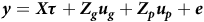 $$\boldsymbol y = X\tau + {Z_g}{u_g} + {Z_p}{u_p} + e$$
where ${\boldsymbol \tau }$
is a vector of fixed effects with associated design matrix
${\boldsymbol \tau }$
is a vector of fixed effects with associated design matrix ${\boldsymbol X}$
;
${\boldsymbol X}$
; ${{\boldsymbol u}_g}$
is the vector of random genetic effects with associated design matrix
${{\boldsymbol u}_g}$
is the vector of random genetic effects with associated design matrix ${{\boldsymbol Z}_g}$
;
${{\boldsymbol Z}_g}$
; ${{\boldsymbol u}_{\boldsymbol p}}$
is a vector of random non-genetic (or peripheral) effects with associated design matrix
${{\boldsymbol u}_{\boldsymbol p}}$
is a vector of random non-genetic (or peripheral) effects with associated design matrix ${{\boldsymbol Z}_p}$
and
${{\boldsymbol Z}_p}$
and ${\boldsymbol e} = {({\boldsymbol e}_1^ \top, {\boldsymbol e}_2^ \top, \ldots, {\boldsymbol e}_p^ \top )^ \top }$
is the combined vector of errors from all environments. The vector of fixed effects includes mean parameters for individual environments. The vector of random peripheral effects includes effects associated with the designs of individual trials within environments. The variance matrix for
${\boldsymbol e} = {({\boldsymbol e}_1^ \top, {\boldsymbol e}_2^ \top, \ldots, {\boldsymbol e}_p^ \top )^ \top }$
is the combined vector of errors from all environments. The vector of fixed effects includes mean parameters for individual environments. The vector of random peripheral effects includes effects associated with the designs of individual trials within environments. The variance matrix for ${{\boldsymbol u}_{\boldsymbol p}}$
is typically given by
${{\boldsymbol u}_{\boldsymbol p}}$
is typically given by ${\boldsymbol G_p} = \oplus _{j = 1}^p{\boldsymbol G_p}_j$
where
${\boldsymbol G_p} = \oplus _{j = 1}^p{\boldsymbol G_p}_j$
where ${\boldsymbol G_p}_j = {\rm{var}}\left( {{{\boldsymbol u}_{\boldsymbol p}}_j} \right)$
and
${\boldsymbol G_p}_j = {\rm{var}}\left( {{{\boldsymbol u}_{\boldsymbol p}}_j} \right)$
and ${{\boldsymbol u}_{\boldsymbol p}}_j$
is the vector of peripheral effects for environment
${{\boldsymbol u}_{\boldsymbol p}}_j$
is the vector of peripheral effects for environment $j$
.
$j$
.
Variance models for genetic effects
The random genetic effects, ${{\boldsymbol u}_g}$
, comprise the variety effects nested within environments (VE effects). In this paper, these effects are partitioned into additive and non-additive genetic effects, so for clarity
${{\boldsymbol u}_g}$
, comprise the variety effects nested within environments (VE effects). In this paper, these effects are partitioned into additive and non-additive genetic effects, so for clarity ${{\boldsymbol u}_g}$
will be referred to as the total VE effects. If
${{\boldsymbol u}_g}$
will be referred to as the total VE effects. If $m$
denotes the total number of unique varieties across all environments, then the vector
$m$
denotes the total number of unique varieties across all environments, then the vector ${{\boldsymbol u}_g}$
has length
${{\boldsymbol u}_g}$
has length $mp$
. These are assumed to be ordered as varieties within environments. The total VE effects can be partitioned into additive and non-additive VE effects (
$mp$
. These are assumed to be ordered as varieties within environments. The total VE effects can be partitioned into additive and non-additive VE effects ( ${{\boldsymbol u}_a}$
and
${{\boldsymbol u}_a}$
and ${{\boldsymbol u}_e}$
, respectively) as follows:
${{\boldsymbol u}_e}$
, respectively) as follows:
 $$\boldsymbol {u_g} = {u_a} + {u_e}$$
where it is assumed that
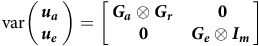 $${\rm{var}}\boldsymbol{ \left( {\matrix{ {{u_a}} \cr {{u_e}} \hfill \cr } } \right) }= \left[ {\matrix{ {{\boldsymbol {G_a}} \otimes {G_r}} & \hskip 2pt {\bf 0} \cr \hskip 2pt {\bf 0} & {{\boldsymbol {G_e}} \otimes {I_m}} } } \right]$$
where $\boldsymbol{\boldsymbol {G_a}}$
and
$\boldsymbol{\boldsymbol {G_a}}$
and $\boldsymbol{\boldsymbol {G_e}}$
are
$\boldsymbol{\boldsymbol {G_e}}$
are $p \times p$
symmetric positive semi-definite matrices that will be referred to as the between environment additive and non-additive genetic variance matrices, respectively. The matrix
$p \times p$
symmetric positive semi-definite matrices that will be referred to as the between environment additive and non-additive genetic variance matrices, respectively. The matrix $\boldsymbol{G_r}$
is an
$\boldsymbol{G_r}$
is an $m \times m$
(known) relationship matrix which may either be an NRM, denoted
$m \times m$
(known) relationship matrix which may either be an NRM, denoted ${\boldsymbol A}$
, or a genomic relationship matrix (GRM). Note that for notational simplicity, it is assumed that pedigree and/or genomic information is available for all
${\boldsymbol A}$
, or a genomic relationship matrix (GRM). Note that for notational simplicity, it is assumed that pedigree and/or genomic information is available for all $m$
varieties. This is easily relaxed in practice. In the current paper, the motivating example involves the use of pedigree information, so the approach is developed in this context, in which case
$m$
varieties. This is easily relaxed in practice. In the current paper, the motivating example involves the use of pedigree information, so the approach is developed in this context, in which case $\boldsymbol G_r = A$
. Note that
$\boldsymbol G_r = A$
. Note that ${\boldsymbol A}$
is often expanded to include both the varieties grown in the MET together with their ancestors (that were not grown in the MET). This may be done both to allow prediction of the additive VE effects for the latter and also to exploit the sparsity it induces in the inverse of the NRM. Either way,
${\boldsymbol A}$
is often expanded to include both the varieties grown in the MET together with their ancestors (that were not grown in the MET). This may be done both to allow prediction of the additive VE effects for the latter and also to exploit the sparsity it induces in the inverse of the NRM. Either way, $m$
is defined to denote the number of varieties with pedigree information which will therefore also be the number of rows and columns in
$m$
is defined to denote the number of varieties with pedigree information which will therefore also be the number of rows and columns in ${\boldsymbol A}$
. Finally, note that
${\boldsymbol A}$
. Finally, note that ${\rm{var}}{\boldsymbol{ \left( {{u_g}} \right)} = {\boldsymbol{\boldsymbol {G_a}}} \otimes {\boldsymbol A} + {\boldsymbol {\boldsymbol {G_e}}} \otimes {{\boldsymbol I}_{\it m}}}$
FA models for VE effects
Given the partitioning of the total VE effects, a separate FA model for each set of VE effects is allowed. Thus, a FA model of order ${k_a}$
, denoted FA
${k_a}$
, denoted FA ${k_a}$
, is assumed for the additive VE effects and an FA
${k_a}$
, is assumed for the additive VE effects and an FA ${k_e}$
model is assumed for the non-additive VE effects. Note that the orders of the two models, that is,
${k_e}$
model is assumed for the non-additive VE effects. Note that the orders of the two models, that is, ${k_a}$
and
${k_a}$
and ${k_e}$
may (are likely to) be different. The FA models for the VE effects can be written as
${k_e}$
may (are likely to) be different. The FA models for the VE effects can be written as
 $${\boldsymbol {u_a}} = \left( {\boldsymbol{{\Lambda _a}} \otimes {{\boldsymbol I}_{\it m}}} \right){\boldsymbol {f_a}} + {\boldsymbol {\delta _a}} = {\bf {\beta _{\it a}}} + {\boldsymbol {\delta _a}}$$
 $${\boldsymbol {u_e}} = \left( {\boldsymbol {{\Lambda _e}} \otimes {{\boldsymbol I}_{\it m}}} \right){\boldsymbol {f_e}} + {\boldsymbol {\delta _e}} = {\bf {\beta _{\it e}}} + {\boldsymbol {\delta _e}}$$
where $\boldsymbol{\Lambda _a}$
is the
$\boldsymbol{\Lambda _a}$
is the $p \times {k_a}$
matrix of environment loadings for the individual additive factors;
$p \times {k_a}$
matrix of environment loadings for the individual additive factors; $\boldsymbol{f_a}$
is the associated
$\boldsymbol{f_a}$
is the associated $m{k_a} - $
vector of variety scores (ordered as varieties within factors) and
$m{k_a} - $
vector of variety scores (ordered as varieties within factors) and $\boldsymbol {\delta _a}$
is the
$\boldsymbol {\delta _a}$
is the $mp - $
vector of additive lack of fit effects which are also known as the additive specific VE (SVE) effects. The additive common VE (CVE) effects are given by
$mp - $
vector of additive lack of fit effects which are also known as the additive specific VE (SVE) effects. The additive common VE (CVE) effects are given by $\boldsymbol{\beta _a} = \left( {{\Lambda _a} \otimes {I_{\it m}}} \right){f_a}$
. The FA model for non-additive VE effects involves
$\boldsymbol{\beta _a} = \left( {{\Lambda _a} \otimes {I_{\it m}}} \right){f_a}$
. The FA model for non-additive VE effects involves $\boldsymbol {\Lambda _e}$
, which is the
$\boldsymbol {\Lambda _e}$
, which is the $p \times {k_e}$
matrix of environment loadings for the individual non-additive factors;
$p \times {k_e}$
matrix of environment loadings for the individual non-additive factors; $\boldsymbol {f_e}$
is the associated
$\boldsymbol {f_e}$
is the associated $m{k_e} - $
vector of variety scores and
$m{k_e} - $
vector of variety scores and ${{\boldsymbol \delta} _e}$
is the
${{\boldsymbol \delta} _e}$
is the $mp - $
vector of non-additive SVE effects. The non-additive CVE effects are given by
$mp - $
vector of non-additive SVE effects. The non-additive CVE effects are given by $\boldsymbol{\beta _{\bf{e}}} = \left( {{\Lambda _e} \otimes {I_{\it m}}} \right){f_e}$
.
$\boldsymbol{\beta _{\bf{e}}} = \left( {{\Lambda _e} \otimes {I_{\it m}}} \right){f_e}$
.
This then provides a model for the total VE effects of the form
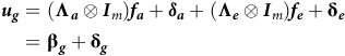 $$\eqalign{{\boldsymbol u_g} =\ & \left( {{\boldsymbol \Lambda _a} \otimes {{\boldsymbol I}_m}} \right){\boldsymbol f_a} + {{\bf \delta} _ {\boldsymbol a}} + \left( {{\boldsymbol \Lambda _e} \otimes {{\boldsymbol I}_m}} \right){\boldsymbol f_e} + {{\bf \delta} _{\boldsymbol e}}\cr=\ & {{{\bf \beta}} _{\boldsymbol g}} + {{{\bf\delta}} _{\boldsymbol g}}}$$
where ${\boldsymbol {\beta _g}} = {\boldsymbol {\beta _a}} + {\boldsymbol {\beta _e}}$
and
${\boldsymbol {\beta _g}} = {\boldsymbol {\beta _a}} + {\boldsymbol {\beta _e}}$
and ${\boldsymbol {\delta _g}} = {\boldsymbol {\delta _a}} + {\boldsymbol {\delta _e}}$
are defined to be the total CVE and total SVE effects, respectively.
${\boldsymbol {\delta _g}} = {\boldsymbol {\delta _a}} + {\boldsymbol {\delta _e}}$
are defined to be the total CVE and total SVE effects, respectively.
In the FA models, it is assumed that
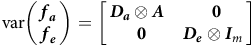 $${\rm{var}}\left( \matrix{ {{\boldsymbol f}_{\boldsymbol a}} \cr {{\boldsymbol f}_{\boldsymbol e}} } \right) = {\left[ {\matrix{ {{{\boldsymbol D}_{\boldsymbol a}} \otimes {\boldsymbol A}} & {\hskip 4pt \bf 0} \cr \hskip 4pt {\bf 0} & {{{\boldsymbol D}_{\boldsymbol e}} \otimes {\boldsymbol I}_m}}} \right]}$$
where $\boldsymbol {D_a}$
and
$\boldsymbol {D_a}$
and $\boldsymbol {D_e}$
are
$\boldsymbol {D_e}$
are ${k_a} \times {k_a}$
and
${k_a} \times {k_a}$
and ${k_e} \times {k_e}$
symmetric positive definite matrices that will be referred to as the additive and non-additive factor score variance matrices, respectively. Additionally, it is assumed that
${k_e} \times {k_e}$
symmetric positive definite matrices that will be referred to as the additive and non-additive factor score variance matrices, respectively. Additionally, it is assumed that
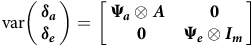 $${\rm{var}}\left( {\matrix{ {\boldsymbol{\delta _a}} \hfill \cr {\boldsymbol{\delta _e}} \hfill \cr } } \right) = \left[ {\matrix{ {{{\bf{\Psi }}_{\boldsymbol a}} \otimes \boldsymbol A} & {\hskip 2pt\bf 0} \cr {\hskip 4pt\bf 0} & {{{\bf{\Psi }}_{\boldsymbol e}} \otimes \boldsymbol {I_m}} \hfill \cr } } \right]$$
where ${{\bf{\Psi }}_{\boldsymbol a}}$
and
${{\bf{\Psi }}_{\boldsymbol a}}$
and ${{\bf{\Psi }}_{\boldsymbol e}}$
are
${{\bf{\Psi }}_{\boldsymbol e}}$
are $p \times p$
diagonal matrices with elements referred to as the additive and non-additive specific variances, respectively.
$p \times p$
diagonal matrices with elements referred to as the additive and non-additive specific variances, respectively.
The variance assumptions in equations (6) and (7) lead to
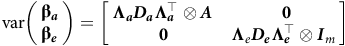 $${\rm{var}}\left( {\matrix{ {{\bf{\beta}_{\boldsymbol a}}} \hfill \cr {{\bf{\beta}_{\boldsymbol e}}} \hfill \cr } } \right) = \left[ {\matrix{ {\boldsymbol {\Lambda _a}{D_a}{{\bf\Lambda }}_{a}^ \top \otimes \boldsymbol A} & {\hskip 4pt \bf 0} \cr {\hskip 1pt \bf 0} & {{{\bf{\Lambda }}_e}{\boldsymbol D_e}{{\bf\Lambda }}_{\boldsymbol e}^ \top \otimes {{\boldsymbol I}_m}} \hfill \cr } } \right]$$
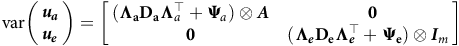 $${\rm{var}}\left( {\matrix{ {\boldsymbol {\textbf u_a}} \hfill \cr {\boldsymbol {\textbf u_e}} \hfill \cr } } \right) = \left[ {\matrix{ {\left( {{\bf {\Lambda} _a}{\bf D_a}{{\bf\Lambda }}_{a}^ \top + {{\bf{\Psi }}_a}} \right) \otimes \boldsymbol A} & {\hskip 4pt \bf 0} \cr {\bf 0} & {\left( {\boldsymbol {\Lambda _e}{\bf D_e}{{\bf\Lambda }}_{e}^ \top + {{\bf{\Psi }}_{\bf{e}}}} \right) \otimes {{\boldsymbol I}_m}} \hfill \cr } } \right]$$
so that the between environment additive and non-additive genetic variance matrices are given by $\boldsymbol {\boldsymbol \bf{G_a}} = {\Lambda _a}{D_a}\Lambda_{a}^\top+ {{\bf{\Psi }}_a}$
and
$\boldsymbol {\boldsymbol \bf{G_a}} = {\Lambda _a}{D_a}\Lambda_{a}^\top+ {{\bf{\Psi }}_a}$
and $\boldsymbol {\boldsymbol {G_e}} = {\Lambda _e}{D_e}\Lambda _{e}^ \top + {{\bf{\Psi }}_e}$
, respectively.
$\boldsymbol {\boldsymbol {G_e}} = {\Lambda _e}{D_e}\Lambda _{e}^ \top + {{\bf{\Psi }}_e}$
, respectively.
Smith et al. (Reference Smith, Norman, Kuchel and Cullis2021b) discussed the need to apply constraints in an FA model in order to ensure a unique solution. Their approach is adopted here and the same form of constraints for both the additive and non-additive FA models is imposed. Thus, it is assumed that the additive factor scores are independent so that $\boldsymbol {D_a}$
is a diagonal (non-identity) matrix with elements
$\boldsymbol {D_a}$
is a diagonal (non-identity) matrix with elements ${d_{{a_r}}}$
(
${d_{{a_r}}}$
( $r = 1 \ldots {k_a}$
), and furthermore, these are written in decreasing order of magnitude. It is also assumed that
$r = 1 \ldots {k_a}$
), and furthermore, these are written in decreasing order of magnitude. It is also assumed that $\boldsymbol\Lambda_{{a}}^ \top{\Lambda _a}$
is an identity matrix (that is, the columns of
$\boldsymbol\Lambda_{{a}}^ \top{\Lambda _a}$
is an identity matrix (that is, the columns of $ \boldsymbol {\Lambda _a}$
are orthonormal vectors). Similarly, it is assumed that the non-additive factor scores are independent so that
$ \boldsymbol {\Lambda _a}$
are orthonormal vectors). Similarly, it is assumed that the non-additive factor scores are independent so that $\boldsymbol {D_e}$
is a diagonal (non-identity) matrix with elements
$\boldsymbol {D_e}$
is a diagonal (non-identity) matrix with elements ${d_{{e_s}}}$
(
${d_{{e_s}}}$
( $s = 1 \ldots {k_e}$
) and these are written in decreasing order of magnitude. It is also assumed that
$s = 1 \ldots {k_e}$
) and these are written in decreasing order of magnitude. It is also assumed that $\boldsymbol \Lambda_{e}^\top {\Lambda _e}$
is an identity matrix. These constraints allow for a meaningful interpretation of loadings and scores (Smith and Cullis, Reference Smith and Cullis2018; Smith et al., Reference Smith, Norman, Kuchel and Cullis2021b). The constraints used for estimation will be discussed in the section ‘Model fitting and estimation’.
$\boldsymbol \Lambda_{e}^\top {\Lambda _e}$
is an identity matrix. These constraints allow for a meaningful interpretation of loadings and scores (Smith and Cullis, Reference Smith and Cullis2018; Smith et al., Reference Smith, Norman, Kuchel and Cullis2021b). The constraints used for estimation will be discussed in the section ‘Model fitting and estimation’.
It is instructive to express the model for the total VE effects in expanded form as follows: write ${\boldsymbol {\Lambda _a}} = \left[ {{{\boldsymbol \lambda} _{{{\boldsymbol a}_1}}}, \ldots, {{\boldsymbol \lambda} _{{{\boldsymbol a}_{{k_a}}}}}} \right]$
where
${\boldsymbol {\Lambda _a}} = \left[ {{{\boldsymbol \lambda} _{{{\boldsymbol a}_1}}}, \ldots, {{\boldsymbol \lambda} _{{{\boldsymbol a}_{{k_a}}}}}} \right]$
where ${{\boldsymbol \lambda} _{{{\boldsymbol a}_r}}}$
is the
${{\boldsymbol \lambda} _{{{\boldsymbol a}_r}}}$
is the $p - $
vector of environment loadings for additive factor
$p - $
vector of environment loadings for additive factor $r$
and write
$r$
and write ${\boldsymbol {f_a}} = {({\boldsymbol f}_{{{\boldsymbol a}_1}}^ \top, \ldots, {\boldsymbol f}_{{{\boldsymbol a}_{{k_a}}}}^ \top )^ \top }$
where
${\boldsymbol {f_a}} = {({\boldsymbol f}_{{{\boldsymbol a}_1}}^ \top, \ldots, {\boldsymbol f}_{{{\boldsymbol a}_{{k_a}}}}^ \top )^ \top }$
where $\boldsymbol {f_{\it{a_r}}}$
is the
$\boldsymbol {f_{\it{a_r}}}$
is the $m - $
vector of variety scores for additive factor
$m - $
vector of variety scores for additive factor $r$
. Analogous definitions are used for the loadings and scores for the non-additive factors. The model in equation (5) can then be written as
$r$
. Analogous definitions are used for the loadings and scores for the non-additive factors. The model in equation (5) can then be written as
 $$\boldsymbol {u_g} = \left( {\bf {\lambda} _{{a_1}} \otimes {\boldsymbol {I}_m}} \right){\boldsymbol {f }_{{a_1}}} + \left( {{\bf {\lambda} _{{a_2}}} \otimes {\boldsymbol {I}_m}} \right){\boldsymbol {f }_{{{a_2}}} + \ldots + \left( {{\boldsymbol {\lambda} _{{\boldsymbol {a}_{{k_a}}}}} \otimes {\boldsymbol {I}_m}} \right){\boldsymbol {f \!}_{{\boldsymbol {a}_{{k_a}}}}} }+$$
 $$ \left( {{{\bf \lambda} _{{e_1}}} \otimes {{\boldsymbol I}_m}} \right){{\boldsymbol f \!}_{{e_1}}} + \left( {{{\bf \lambda} _{{e_2}}} \otimes {{\boldsymbol I}_m}} \right){{\boldsymbol f \!}_{{e_2}}} + \ldots + \left( {{{\bf \lambda} _{{{\boldsymbol e}_{{k_e}}}}} \otimes {{\boldsymbol I}_m}} \right){\boldsymbol f_{{e_{\it {k_e}}}}} + {{\boldsymbol \delta _g}}$$
which has the appearance of a multiple regression with $k = {k_a} + {k_e}$
terms in which the covariates are the loadings (
$k = {k_a} + {k_e}$
terms in which the covariates are the loadings ( ${{\boldsymbol \lambda} _a}_r$
and
${{\boldsymbol \lambda} _a}_r$
and ${{\boldsymbol \lambda} _e}_s$
) and there are separate slopes for individual varieties which are given by the variety scores (
${{\boldsymbol \lambda} _e}_s$
) and there are separate slopes for individual varieties which are given by the variety scores ( ${\boldsymbol {f_a}}_r$
and
${\boldsymbol {f_a}}_r$
and ${\boldsymbol {f_e}}_s$
).
${\boldsymbol {f_e}}_s$
).
The percentage of variance accounted for by each factor in the overall model of equation (10) can be obtained using the results in the Appendix. Thus the percentages of variance accounted for by additive factor $r$
(
$r$
( $ = 1 \ldots {k_a}$
) and non-additive factor
$ = 1 \ldots {k_a}$
) and non-additive factor $s$
(
$s$
( $ = 1 \ldots {k_e}$
) are given by
$ = 1 \ldots {k_e}$
) are given by
 $${V_{{a_r}}} = 100 \times \bar a{d_{{a_r}}}/{\rm{tr}}\left( {\bar a\boldsymbol {\boldsymbol {G_a}} + {\boldsymbol {G_e}}} \right)$$
 $${V_{{e_s}}} = 100 \times {d_{{e_s}}}/{\rm{tr}}\left( {\bar a\boldsymbol {\boldsymbol {G_a}} + {\boldsymbol {G_e}}} \right)$$
where $\bar a$
is (typically) the mean of the diagonal elements of
$\bar a$
is (typically) the mean of the diagonal elements of $\boldsymbol A$
for those varieties that were grown in the MET or alternatively the subset under consideration for selection. By definition, the additive factor score variances are in decreasing order so that
$\boldsymbol A$
for those varieties that were grown in the MET or alternatively the subset under consideration for selection. By definition, the additive factor score variances are in decreasing order so that ${V_{{a_1}}} \gt {V_{{a_2}}} \gt \ldots \gt {V_{{a_{{k_a}}}}}$
. Similarly, the non-additive factor score variances are in decreasing order so that
${V_{{a_1}}} \gt {V_{{a_2}}} \gt \ldots \gt {V_{{a_{{k_a}}}}}$
. Similarly, the non-additive factor score variances are in decreasing order so that ${V_{{e_1}}} \gt {V_{{e_2}}} \gt \ldots \gt {V_{{e_{{k_e}}}}}$
. However, the overall ordering of factors (that is, across additive and non-additive) is data-dependent.
${V_{{e_1}}} \gt {V_{{e_2}}} \gt \ldots \gt {V_{{e_{{k_e}}}}}$
. However, the overall ordering of factors (that is, across additive and non-additive) is data-dependent.
Variance models for errors
The reader is referred to the Supplementary Material, Section 2.
Model fitting and estimation
Every model in this paper was fitted using DWReml which is a package within the R statistical software (R Core Team, 2022). DWReml fits the LMM and estimates variance parameters using residual maximum likelihood (REML) (Patterson and Thompson, 1971) and the average information algorithm and a supernodal sparse linear solver. The models could also have been fitted using the commercially available software ASReml-R (Butler et al., Reference Butler, Cullis, Gilmour, Gogel and Thompson2017). The models required a NRM and this was created from pedigree records using pedicure which is a package within the R statistical software (R Core Team, 2022) that provides tools for pedigrees and genetic marker matrices. Both DWReml and pedicure were developed by David Butler and Brian Cullis. Beta versions are freely available from Brian Cullis (bcullis@uow.edu.au) on request.
The FA variance models were fitted as in Smith and Cullis (Reference Smith and Cullis2018), that is, by splitting the VE effects into the CVE and SVE effects, each with their own variance structure. Thus, for the additive VE effects the two variance models were ${{var}}\left( {\boldsymbol {{{\bf \beta}} _a}} \right)$
and
${{var}}\left( {\boldsymbol {{{\bf \beta}} _a}} \right)$
and ${\rm{var}}\left( {\boldsymbol {\delta _a}} \right)$
as given in equations (8) and (7). The two variance models for the non-additive VE effects were
${\rm{var}}\left( {\boldsymbol {\delta _a}} \right)$
as given in equations (8) and (7). The two variance models for the non-additive VE effects were ${\rm{var}}\left( {\boldsymbol {{\bf {\beta}} _e}} \right)$
and
${\rm{var}}\left( {\boldsymbol {{\bf {\beta}} _e}} \right)$
and ${\rm{var}}\left( {\boldsymbol {\delta _e}} \right)$
as given in equations (8) and (7).
${\rm{var}}\left( {\boldsymbol {\delta _e}} \right)$
as given in equations (8) and (7).
As discussed in Smith et al. (Reference Smith, Norman, Kuchel and Cullis2021b), model fitting using the constraints on loadings and factor score variances as outlined in the section ‘FA models for VE effects’ is difficult and both DWReml and ASReml-R (Butler et al., Reference Butler, Cullis, Gilmour, Gogel and Thompson2017) use simpler constraints. These involve setting ${{\boldsymbol D_a}} = {{\boldsymbol I}_{{k_a}}}$
and
${{\boldsymbol D_a}} = {{\boldsymbol I}_{{k_a}}}$
and ${\boldsymbol D_e} = {{\boldsymbol I}_{{k_e}}}$
. Additionally, if
${\boldsymbol D_e} = {{\boldsymbol I}_{{k_e}}}$
. Additionally, if ${k_a} \gt 1$
, then all the elements in the upper triangle of
${k_a} \gt 1$
, then all the elements in the upper triangle of ${{\boldsymbol \Lambda _a}}$
are set to zero. If
${{\boldsymbol \Lambda _a}}$
are set to zero. If ${k_e} \gt 1$
, the same constraints are applied to the non-additive loadings. The original forms of the loading and score variance matrices can be reconstructed using a rotation based on a singular value decomposition of the associated loading matrix. The reader is referred to Smith et al. (Reference Smith, Norman, Kuchel and Cullis2021b) for full details.
${k_e} \gt 1$
, the same constraints are applied to the non-additive loadings. The original forms of the loading and score variance matrices can be reconstructed using a rotation based on a singular value decomposition of the associated loading matrix. The reader is referred to Smith et al. (Reference Smith, Norman, Kuchel and Cullis2021b) for full details.
Note that two separate rotations are conducted, corresponding to the additive and non-additive factor models. This is to be contrasted with the approach proposed in Smith and Cullis (Reference Smith and Cullis2018) in which the columns in the additive and non-additive loading matrices are combined to form an overall matrix of loadings to which a single rotation is applied. The authors claimed this provides a ‘special FA form’ for the total VE effects. However, the two models are not compatible, because the factor scores in the additive model have a variance structure that involves a relationship matrix whereas the factor scores in the non-additive model are independent. The single rotation then mixes the variance structures in a manner that is both unclear and results in scores that are correlated across factors. The separate rotations used in the current paper ensure that the joint factor score variance matrix remains as in equation (6), so that in terms of the regression implicit in equation (10), the slopes (scores) for an individual variety are independent (uncorrelated) across all $k$
terms. This allows for uncomplicated interpretations of the variety scores. Furthermore, the use of two separate rotations is consistent with the fundamental reason for the rotations, namely to move away from the computationally convenient constraints imposed for uniqueness. The constraints only apply within an individual FA model so that two separate rotations are required, corresponding to the additive and non-additive loading matrices. In this context, it is helpful to consider that in the simplest case where each of the two-factor models comprises a single factor, there is no need for any rotation.
$k$
terms. This allows for uncomplicated interpretations of the variety scores. Furthermore, the use of two separate rotations is consistent with the fundamental reason for the rotations, namely to move away from the computationally convenient constraints imposed for uniqueness. The constraints only apply within an individual FA model so that two separate rotations are required, corresponding to the additive and non-additive loading matrices. In this context, it is helpful to consider that in the simplest case where each of the two-factor models comprises a single factor, there is no need for any rotation.
The model fit provides REML estimates of all variance parameters and empirical best linear unbiased predictions (EBLUPs) of all random effects.
Variety selection using interaction classes
In cases where the aim is selection based on additive effects alone, the iClass approach of Smith et al. (Reference Smith, Norman, Kuchel and Cullis2021b) can be directly applied to the FA model for the additive VE effects. For example in the analysis of data for inbred crops, such as lentils, there may be interest in using the additive effects for the selection of potential new parental lines. The iClass technique of Smith et al. (Reference Smith, Norman, Kuchel and Cullis2021b) applied to additive VE effects could also be used in cases where the LMM does not include non-additive effects, such as the analysis of out-crossing species.
The extension of Smith et al. (Reference Smith, Norman, Kuchel and Cullis2021b) considered here relates to the selection of superior varieties in terms of their total (additive plus non-additive) VE effects. iClasses for this purpose can be formed by first ordering all $k = {k_a} + {k_e}$
factors in terms of their percentage variance accounted for, namely using
$k = {k_a} + {k_e}$
factors in terms of their percentage variance accounted for, namely using ${V_{{a_r}}}$
and
${V_{{a_r}}}$
and ${V_{{e_s}}}$
of equation (11). As discussed in the section ‘FA models for VE effects’, the factors are already in order of variance accounted for within their respective FA models, but the ordering across additive and non-additive factors may result in a mixing of the two types. The factor loadings ordered in this way are denoted by
${V_{{e_s}}}$
of equation (11). As discussed in the section ‘FA models for VE effects’, the factors are already in order of variance accounted for within their respective FA models, but the ordering across additive and non-additive factors may result in a mixing of the two types. The factor loadings ordered in this way are denoted by ${{\boldsymbol \lambda}_t}$
(
${{\boldsymbol \lambda}_t}$
( $t = 1 \ldots k$
). The corresponding vectors of factor scores are denoted by
$t = 1 \ldots k$
). The corresponding vectors of factor scores are denoted by ${{\boldsymbol f \!}_t}$
.
${{\boldsymbol f \!}_t}$
.
At this point, it is instructive to clarify the logic behind the iClass concept introduced in Smith et al. (Reference Smith, Norman, Kuchel and Cullis2021b). The key is to use the regression interpretation of an FA model for VE effects. In the current paper in which there is a separate FA model for the additive and non-additive VE effects, the regression interpretation stems from equation (10). Using the notation just defined for indexing factors across additive and non-additive terms, the fitted values from this regression for variety $i$
in environment
$i$
in environment $j$
are given by
$j$
are given by
 $${\tilde {\rm \beta} _{{g_{ij}}}} = {\hat {\rm \lambda} _{1j}}\,{\tilde f_{i1}} + {\hat{\rm \lambda} _{2j}}\,{\tilde f_{i2}} + \ldots {\hat {\rm \lambda} _{kj}}\,{\tilde f_{ik}}$$
where the hat symbol above a variance parameter indicates the REML estimate of the parameter and the tilde symbol above a random effect indicates the EBLUP of the effect. A visual assessment of the contribution of an individual factor (term in the regression) to the overall fitted value aids in the explanation of iClasses. A hypothetical example comprising $k = 3$
factors fitted to
$k = 3$
factors fitted to $p = 9$
environments is considered. Figure 1 shows, for three varieties (v1, v2 and v3), the fitted values for each factor (that is,
$p = 9$
environments is considered. Figure 1 shows, for three varieties (v1, v2 and v3), the fitted values for each factor (that is, ${\hat {\rm \lambda} _{tj}}\,{\tilde f_{it}}$
) plotted against the covariate (the rotated estimated environment loadings,
${\hat {\rm \lambda} _{tj}}\,{\tilde f_{it}}$
) plotted against the covariate (the rotated estimated environment loadings, ${\hat {\rm \lambda} _{tj}}$
for the factor). The slopes of the lines are the EBLUPs of the variety scores (
${\hat {\rm \lambda} _{tj}}$
for the factor). The slopes of the lines are the EBLUPs of the variety scores ( ${\tilde f_{1t}},{\tilde f_{2t}}$
and
${\tilde f_{1t}},{\tilde f_{2t}}$
and ${\tilde f_{3t}}$
) for the factor.
${\tilde f_{3t}}$
) for the factor.
In this example, the first factor contains all positive estimated loadings and it is clear from Figure 1a that there are no crossover interactions of varieties for any environments. Thus in terms of the fitted values for the first factor, variety v1 always ranks first, followed by v2 then v3. The second and third factors are bi-polar, with mixtures of positive and negative estimated loadings. Figure 1b and c show that, for all environments that have the same sign for the estimated loadings (either positive or negative), there is no crossover interaction between varieties in terms of the fitted values for the associated factor. Thus for the second factor (see Figure 1b) variety v2 ranks first, v3 second and v1 last for all environments with a positive estimated loading (e4 and e1) and variety v1 ranks first, v3 second and v2 last for all environments with negative loadings (the remainder). Clearly, the crossovers (rank changes) occur at the origin (indicated by a dashed vertical line). Thus for any pair of environments that differ in the signs of their estimated loadings (so positive versus negative), there are changes in variety rankings. These two, but dual, phenomenon provide the motivation for using the signs of estimated loadings to allocate environments into iClasses.
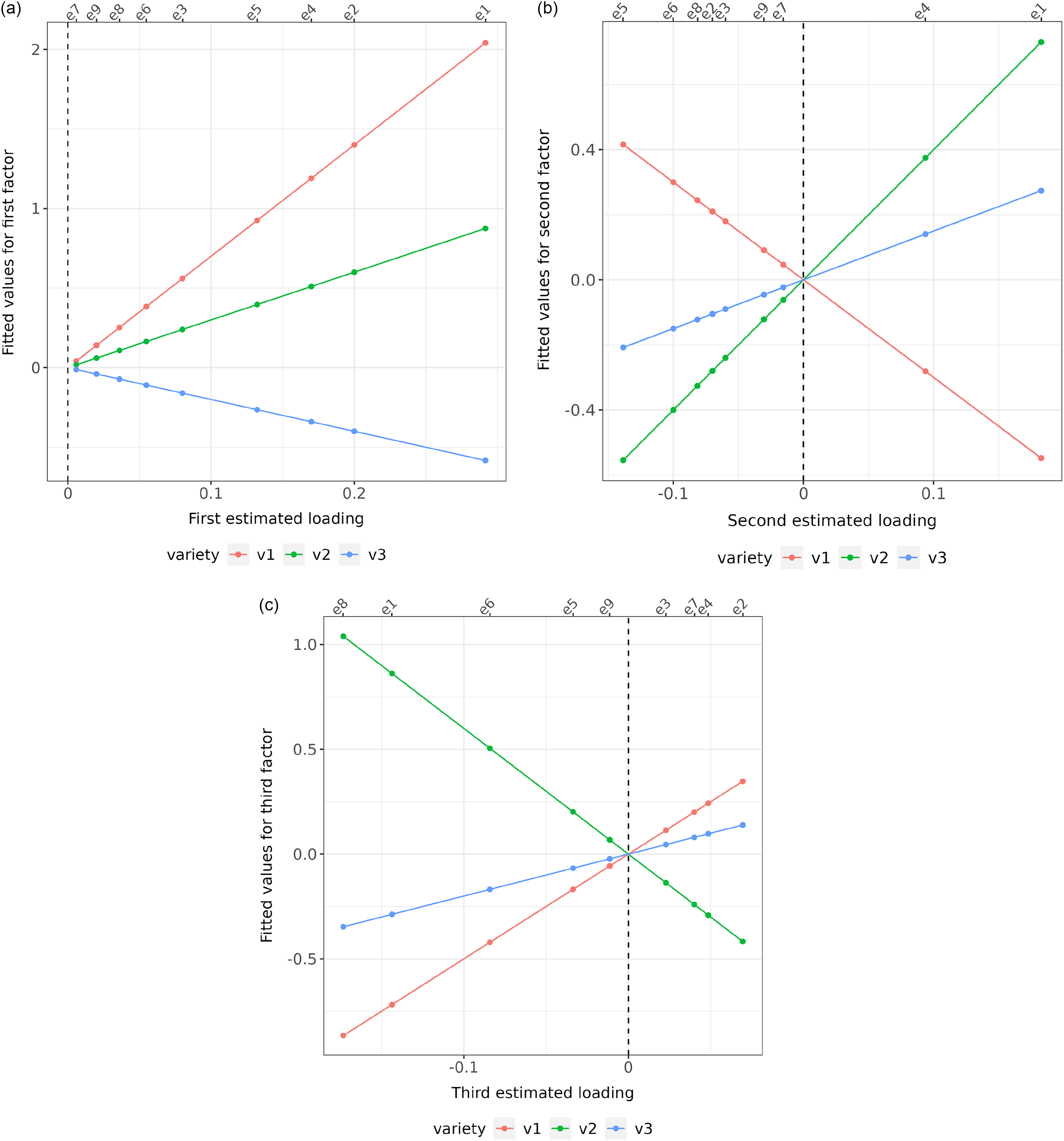
Figure 1. Factor analytic regression model for hypothetical example: fitted values for three varieties (v1, v2 and v3) from model with three factors and nine environments. Fitted values (represented as points) are plotted against estimated factor loadings for individual factors (panels (a), (b) and (c)). The slopes of the regression lines are the empirical best linear unbiased predictions of factor scores for each variety. The residual maximum likelihood estimates of the (rotated) loadings are shown along the bottom axis, and the associated environments are labelled along the top axis.
Specifically, as in Smith et al. (Reference Smith, Norman, Kuchel and Cullis2021b), the REML estimates of the (ordered) loadings are mapped to categorical variables which reflect the signs of the estimates. Formally, for the $t^{th}$
factor loading, the variable
$t^{th}$
factor loading, the variable ${{\boldsymbol S}_t}$
is defined and has only two possible values for environment
${{\boldsymbol S}_t}$
is defined and has only two possible values for environment $j$
(
$j$
( $j = 1 \ldots p$
):
$j = 1 \ldots p$
):
iClasses are then formed from all possible combinations of the values (‘p’ or ‘n’) of the categorical variables ${{\boldsymbol S}_t}$
. Thus, for example, if the total number of additive and non-additive factors is
${{\boldsymbol S}_t}$
. Thus, for example, if the total number of additive and non-additive factors is $k = 3$
, there is a maximum of
$k = 3$
, there is a maximum of ${2^3} = 8$
possible iClasses with the set of labels given by
${2^3} = 8$
possible iClasses with the set of labels given by ${\rm{\Omega }} = \{ $
ppp, ppn, pnp, pnn, npp, npn, nnp, nnn
${\rm{\Omega }} = \{ $
ppp, ppn, pnp, pnn, npp, npn, nnp, nnn $\} $
. Not all of the iClasses may be present in the data. In the hypothetical example, only four of the possible eight iClasses are present, namely ppp (comprising environment e4), ppn (environment e1), pnp (environments e2, e3 and e7) and pnn (environments e5, e6, e8 and e9). It is important to note that the ordering of the characters that form the labels corresponds to the order of importance (in terms of percentage variance accounted for) of the factors (across both additive and non-additive factors).
$\} $
. Not all of the iClasses may be present in the data. In the hypothetical example, only four of the possible eight iClasses are present, namely ppp (comprising environment e4), ppn (environment e1), pnp (environments e2, e3 and e7) and pnn (environments e5, e6, e8 and e9). It is important to note that the ordering of the characters that form the labels corresponds to the order of importance (in terms of percentage variance accounted for) of the factors (across both additive and non-additive factors).
Interaction classes: variety performance
Overall variety performance measures for individual iClasses (iClassOP) can then be computed. The iClassOP for variety $i$
in iClass
$i$
in iClass ${\rm{\omega }}$
(
${\rm{\omega }}$
( ${\rm{\omega }} \in {\rm{\Omega }}$
) is given by
${\rm{\omega }} \in {\rm{\Omega }}$
) is given by
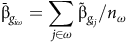 $${\bar {\rm \beta}_{{g_{i\omega }}}} = \mathop \sum \limits_{j \in \omega } {\tilde {\rm \beta} _{{g_{ij}}}}/{n_\omega }$$
where ${n_{\rm \omega} }$
is the number of environments in iClass
${n_{\rm \omega} }$
is the number of environments in iClass ${\rm \omega} $
and the sum is taken over those environments. Using equation (12), the iClassOP in equation (14) can be expressed as
${\rm \omega} $
and the sum is taken over those environments. Using equation (12), the iClassOP in equation (14) can be expressed as
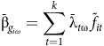 $${\bar {\rm \beta} _{{g_{i\omega }}}} = \mathop \sum \limits_{t = 1}^k {\bar {\rm \lambda} _{t{\rm \omega} }}\,{\tilde f_{it}}$$
where ${\bar {\rm \lambda} _{t{\rm \omega} }} = \mathop \sum \nolimits_{j \in {\rm \omega} } {\hat {\rm \lambda} _{tj}}/{n_{\rm \omega} }$
is the mean of the REML estimates of the loadings for factor
${\bar {\rm \lambda} _{t{\rm \omega} }} = \mathop \sum \nolimits_{j \in {\rm \omega} } {\hat {\rm \lambda} _{tj}}/{n_{\rm \omega} }$
is the mean of the REML estimates of the loadings for factor $t$
for all environments in iClass
$t$
for all environments in iClass ${\rm \omega} $
.
${\rm \omega} $
.
The fact that ${\tilde {\rm \beta} _{{g_{ij}}}} = \mathop \sum \nolimits_{t = 1}^k {\hat \lambda _{tj}}\,{\tilde f_{it}}$
, means that the only random effects associated with the CVEs are the factor scores. This has important implications for the model-based reliability of
${\tilde {\rm \beta} _{{g_{ij}}}} = \mathop \sum \nolimits_{t = 1}^k {\hat \lambda _{tj}}\,{\tilde f_{it}}$
, means that the only random effects associated with the CVEs are the factor scores. This has important implications for the model-based reliability of ${\tilde {\rm \beta} _{{g_{ij}}}}$
. In particular, for any given variety, this reliability is unaffected by the presence or absence of that variety in the environment. In fact, if
${\tilde {\rm \beta} _{{g_{ij}}}}$
. In particular, for any given variety, this reliability is unaffected by the presence or absence of that variety in the environment. In fact, if $k = 1$
, the model-based reliabilities of
$k = 1$
, the model-based reliabilities of ${\tilde {\rm \beta} _{{g_{ij}}}}$
for variety
${\tilde {\rm \beta} _{{g_{ij}}}}$
for variety $i$
are identical for all environments (
$i$
are identical for all environments ( $j = 1 \ldots p$
) in the MET dataset. This has flow-on implications for the reliabilities of iClassOP for any given variety since they are therefore unaffected by the number of environments (including zero) in which the variety is present in that iClass.
$j = 1 \ldots p$
) in the MET dataset. This has flow-on implications for the reliabilities of iClassOP for any given variety since they are therefore unaffected by the number of environments (including zero) in which the variety is present in that iClass.
Interaction classes: variety stability
Smith et al. (Reference Smith, Norman, Kuchel and Cullis2021b) provided the framework for computing iClass overall performance but did not explicitly discuss the concept of stability of variety performance. Their interaction plot enables an investigation of variety stability across iClasses but this is limited to the small number of varieties that can be sensibly displayed on a single plot and is purely a graphical tool. An explicit measure that captures this stability is developed in this paper. The first step involves the choice of iClasses across which stability is to be investigated. This is determined by the breeder and may involve exclusion of iClasses that do not align with their specific selection criteria. The number of iClasses chosen for the stability measure will be denoted by $c$
and the associated number of environments by
$c$
and the associated number of environments by ${p^{\rm{*}}}\left( { \le p} \right)$
. Stability is then investigated for variety
${p^{\rm{*}}}\left( { \le p} \right)$
. Stability is then investigated for variety $i$
using a one-way analysis of variance (AOV) of the
$i$
using a one-way analysis of variance (AOV) of the ${\tilde {\rm \beta} _{{g_{ij}}}}$
values for those environments and with the ‘treatments’ being the
${\tilde {\rm \beta} _{{g_{ij}}}}$
values for those environments and with the ‘treatments’ being the $c$
iClasses. In the AOV table for variety
$c$
iClasses. In the AOV table for variety $i,$
the ‘Between treatment (iClass)’ degrees of freedom are
$i,$
the ‘Between treatment (iClass)’ degrees of freedom are $c - 1$
and the sum of squares is given by
$c - 1$
and the sum of squares is given by
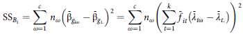 $${{\rm{SS}}_{{B_i}}} = \mathop \sum \limits_{\omega = 1}^c \,{n_\omega }{\left( {{{\bar {\rm \beta} }_{{g_{i\omega }}}} - {{\bar {\rm \beta} }_{{g_{i.}}}}} \right)^2} = \mathop \sum \limits_{\omega = 1}^c {n_\omega }{\left( {\mathop \sum \limits_{t = 1}^k {{\tilde f}_{it}}\left( {{{\bar \lambda }_{t{\rm \omega} }} - {{\bar \lambda }_{t.}}} \right)} \right)^2}$$
where ${\bar {\rm \beta} _{{g_{i.}}}} = \mathop \sum \nolimits_{{\rm \omega} = 1}^c \mathop \sum \nolimits_{j \in {\rm \omega} } {\tilde {\rm \beta} _{{g_{ij}}}}/{p^{\rm{*}}}$
, which is the grand mean of the CVEs, and
${\bar {\rm \beta} _{{g_{i.}}}} = \mathop \sum \nolimits_{{\rm \omega} = 1}^c \mathop \sum \nolimits_{j \in {\rm \omega} } {\tilde {\rm \beta} _{{g_{ij}}}}/{p^{\rm{*}}}$
, which is the grand mean of the CVEs, and ${\bar {\rm \lambda} _{t.}} = \mathop \sum \nolimits_{{\rm \omega} = 1}^c \mathop \sum \nolimits_{j \in {\rm \omega} } {\hat {\rm \lambda} _{tj}}/{p^{\rm{*}}}$
, which is the mean of all loadings for a factor. The between treatment mean square, namely
${\bar {\rm \lambda} _{t.}} = \mathop \sum \nolimits_{{\rm \omega} = 1}^c \mathop \sum \nolimits_{j \in {\rm \omega} } {\hat {\rm \lambda} _{tj}}/{p^{\rm{*}}}$
, which is the mean of all loadings for a factor. The between treatment mean square, namely ${\rm{\;}}{{\rm{SS}}_{{B_i}}}/\left( {c - 1} \right)$
, then measures the variation in treatment means of
${\rm{\;}}{{\rm{SS}}_{{B_i}}}/\left( {c - 1} \right)$
, then measures the variation in treatment means of ${\tilde {\rm \beta} _{{g_{ij}}}}$
(which by definition are the iClassOP), around the grand mean of
${\tilde {\rm \beta} _{{g_{ij}}}}$
(which by definition are the iClassOP), around the grand mean of ${\tilde {\rm \beta} _{{g_{ij}}}}$
. This provides a natural and meaningful measure of the stability of the variety’s performance across relevant iClasses. The ‘Within treatment (iClass)’ degrees of freedom are
${\tilde {\rm \beta} _{{g_{ij}}}}$
. This provides a natural and meaningful measure of the stability of the variety’s performance across relevant iClasses. The ‘Within treatment (iClass)’ degrees of freedom are ${p^{\rm{*}}} - c$
and the sum of squares is given by
${p^{\rm{*}}} - c$
and the sum of squares is given by
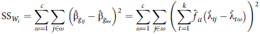 $${{\rm{SS}}_{{W_i}}} = \mathop \sum \limits_{\omega = 1}^c \mathop \sum \limits_{j \in \omega } {\left( {{{\tilde {\rm \beta} }_{{g_{ij}}}} - {{\bar {\rm \beta} }_{{g_{i\omega }}}}} \right)^2} = \mathop \sum \limits_{\omega = 1}^c \mathop \sum \limits_{j \in \omega } {\left( {\mathop \sum \limits_{t = 1}^k {{\tilde f}_{it}}\left( {{{\hat {\rm \lambda} }_{tj}} - {{\bar {\rm \lambda} }_{t\omega }}} \right)} \right)^2}$$
The AOV variance ratio, namely $\left[ {{\rm {SS}}{_{{B_i}}}/\left( {c - 1} \right)\left] / \right[SS{_{{W_i}}}/\left( {{p^{\rm{*}}} - c} \right)} \right]$
, measures the magnitude of variation in CVEs between environments in different iClasses relative to that between environments in the same iClass. As such, when considered collectively across varieties, the variance ratios provide an indication of the effectiveness of the grouping of environments encapsulated in iClass formation. To eliminate issues in summarising variance ratios with large differences in scale it is proposed to consider
$\left[ {{\rm {SS}}{_{{B_i}}}/\left( {c - 1} \right)\left] / \right[SS{_{{W_i}}}/\left( {{p^{\rm{*}}} - c} \right)} \right]$
, measures the magnitude of variation in CVEs between environments in different iClasses relative to that between environments in the same iClass. As such, when considered collectively across varieties, the variance ratios provide an indication of the effectiveness of the grouping of environments encapsulated in iClass formation. To eliminate issues in summarising variance ratios with large differences in scale it is proposed to consider $p - $
values obtained using the approximation of an F-distribution on
$p - $
values obtained using the approximation of an F-distribution on $c - 1$
and
$c - 1$
and ${p^{\rm{*}}} - c$
degrees of freedom, since the
${p^{\rm{*}}} - c$
degrees of freedom, since the $p - $
values are bounded both above and below.
$p - $
values are bounded both above and below.
In this paper, the option of using only the first ${k^{\rm{*}}} \lt k$
ordered factors to form iClasses is considered. Note that, irrespective of the number of factors used to define iClasses, all
${k^{\rm{*}}} \lt k$
ordered factors to form iClasses is considered. Note that, irrespective of the number of factors used to define iClasses, all $k$
factors are used to form
$k$
factors are used to form ${\tilde {\rm \beta} _{{g_{ij}}}}$
and thence iClassOP (equation 15). The use of
${\tilde {\rm \beta} _{{g_{ij}}}}$
and thence iClassOP (equation 15). The use of ${k^{\rm{*}}} \lt k$
factors may be necessary when high order models have been fitted so that the use of all
${k^{\rm{*}}} \lt k$
factors may be necessary when high order models have been fitted so that the use of all $k$
factors to define iClasses may lead to poor membership, that is, small values of
$k$
factors to define iClasses may lead to poor membership, that is, small values of ${n_{\rm \omega} }$
. It may also lead to pairs of iClasses in which differences in variety responses are not sufficiently large to be of importance to the breeder. In such cases, iClasses may be ‘merged’ or more generally only the first few factors may be used to define the iClasses. Such decisions should be driven by the breeder. The individual variety AOV described above may aid in this decision, since the use of too few factors in defining iClasses may lead to a preponderance of large
${n_{\rm \omega} }$
. It may also lead to pairs of iClasses in which differences in variety responses are not sufficiently large to be of importance to the breeder. In such cases, iClasses may be ‘merged’ or more generally only the first few factors may be used to define the iClasses. Such decisions should be driven by the breeder. The individual variety AOV described above may aid in this decision, since the use of too few factors in defining iClasses may lead to a preponderance of large $p$
-values, suggesting that variation in CVEs between environments within an iClass is too large compared with variation between environments in different iClasses.
$p$
-values, suggesting that variation in CVEs between environments within an iClass is too large compared with variation between environments in different iClasses.
Results
The analysis commenced with the use of a LMM in which both ${\boldsymbol {\boldsymbol {G_a}}}$
and
${\boldsymbol {\boldsymbol {G_a}}}$
and ${\boldsymbol {\boldsymbol {G_e}}}$
was assumed to be diagonal matrices. This is analogous to analysing each environment separately and is often used as a baseline to establish appropriate models for the non-genetic effects and errors prior to fitting the more complex FA models. Within the baseline model, random effects for replicate blocks aligned with columns were fitted for all correlation blocks (see Supplementary Material, Section 2 for a definition), as were random effects for rows and columns. Random effects for replicate blocks aligned with rows within correlation blocks were fitted for 32 environments and random effects for correlation blocks were fitted for 57 environments. The only fixed effects fitted were environment main effects. In terms of the spatial modelling of errors, separable (column by row) autoregressive models of order one (denoted AR1 × AR1) were used for all environments. The baseline model was also important for establishing the relative magnitude of the additive VE effects compared with non-additive. The percentage of estimated genetic variance explained by the additive effects for individual environments (see equation A2 in the Appendix), was substantial, with a median of 82 %. This information is of use in the FA modelling process in the sense of indicating that the order of FA models will need to be higher for the additive VE effects compared with non-additive.
${\boldsymbol {\boldsymbol {G_e}}}$
was assumed to be diagonal matrices. This is analogous to analysing each environment separately and is often used as a baseline to establish appropriate models for the non-genetic effects and errors prior to fitting the more complex FA models. Within the baseline model, random effects for replicate blocks aligned with columns were fitted for all correlation blocks (see Supplementary Material, Section 2 for a definition), as were random effects for rows and columns. Random effects for replicate blocks aligned with rows within correlation blocks were fitted for 32 environments and random effects for correlation blocks were fitted for 57 environments. The only fixed effects fitted were environment main effects. In terms of the spatial modelling of errors, separable (column by row) autoregressive models of order one (denoted AR1 × AR1) were used for all environments. The baseline model was also important for establishing the relative magnitude of the additive VE effects compared with non-additive. The percentage of estimated genetic variance explained by the additive effects for individual environments (see equation A2 in the Appendix), was substantial, with a median of 82 %. This information is of use in the FA modelling process in the sense of indicating that the order of FA models will need to be higher for the additive VE effects compared with non-additive.
The non-genetic and error models identified from the fit of the baseline model were carried through (and re-estimated) to the LMMs with FA forms for ${\boldsymbol {G_a}}$
and
${\boldsymbol {G_a}}$
and ${\boldsymbol {G_e}}$
. The models fitted comprised FA models of increasing order from one to four for the additive effects (so
${\boldsymbol {G_e}}$
. The models fitted comprised FA models of increasing order from one to four for the additive effects (so ${k_a} = 1 \ldots 4$
) and an FA model of order one for the non-additive effects (so
${k_a} = 1 \ldots 4$
) and an FA model of order one for the non-additive effects (so ${k_e} = 1$
). A summary of the model fits is provided in Table 2. This table includes all the FA models and the baseline model with diagonal forms for
${k_e} = 1$
). A summary of the model fits is provided in Table 2. This table includes all the FA models and the baseline model with diagonal forms for ${\boldsymbol {G_a}}$
and
${\boldsymbol {G_a}}$
and ${\boldsymbol {G_e}}$
(model M2). Model M1 was fitted in order to assess the impact of using information on genetic relatedness. This model has a diagonal form for
${\boldsymbol {G_e}}$
(model M2). Model M1 was fitted in order to assess the impact of using information on genetic relatedness. This model has a diagonal form for ${\boldsymbol {G_e}}$
but there is no
${\boldsymbol {G_e}}$
but there is no ${\boldsymbol {G_a}}$
. The residual log-likelihoods in Table 2 are expressed as deviations from this model. The benefits in using pedigree information are substantial, with an increase in residual log-likelihood of 4089 (for an additional 90 variance parameters) for model M2 over M1. The addition of genetic covariances between environments is also clearly important, with an increase in residual log-likelihood of 4279 for model M3 over M2 (for an additional 180 variance parameters). Amongst the FA models, the residual log-likelihoods increased as
${\boldsymbol {G_a}}$
. The residual log-likelihoods in Table 2 are expressed as deviations from this model. The benefits in using pedigree information are substantial, with an increase in residual log-likelihood of 4089 (for an additional 90 variance parameters) for model M2 over M1. The addition of genetic covariances between environments is also clearly important, with an increase in residual log-likelihood of 4279 for model M3 over M2 (for an additional 180 variance parameters). Amongst the FA models, the residual log-likelihoods increased as ${k_a}$
was increased, as did the total variance accounted for. Use of the Akaike Information Criteria (AIC) showed that of the models fitted, the final model provided the best fit. The AIC values decline from model M1 to M6 but the rate of decline slows dramatically as the higher models are considered so it is clear that continuing to fit higher-order models will result in smaller gains in terms of goodness-of-fit. Care must be taken when using the AIC to determine the order of FA model as there is a tendency for AIC to keep favouring higher-order models, the upper limit of which is the most general model, known as the unstructured (US) model. A key issue is that the driver for the choice of FA model in a MET context should be to maximise the reliability of variety predictions rather than the goodness-of-fit of the model. Kelly et al. (Reference Kelly, Smith, Eccleston and Cullis2007) showed in a series of simulations for datasets with 7 and 10 environments that FA models of order one or two were generally the preferred model in terms of prediction reliability compared with the US model, even for a number of datasets where the underlying variance structure was generated from a US model. The inferior performance of the US model was associated with instability in variance parameter estimation, due mainly to the large number of variance parameters. The implication is that high order FA models that contain many variance parameters may be similarly affected. This is an unresolved issue but, given the complexity of the lentil dataset, a conservative position was taken to cease the model fitting process at model M6, with
${k_a}$
was increased, as did the total variance accounted for. Use of the Akaike Information Criteria (AIC) showed that of the models fitted, the final model provided the best fit. The AIC values decline from model M1 to M6 but the rate of decline slows dramatically as the higher models are considered so it is clear that continuing to fit higher-order models will result in smaller gains in terms of goodness-of-fit. Care must be taken when using the AIC to determine the order of FA model as there is a tendency for AIC to keep favouring higher-order models, the upper limit of which is the most general model, known as the unstructured (US) model. A key issue is that the driver for the choice of FA model in a MET context should be to maximise the reliability of variety predictions rather than the goodness-of-fit of the model. Kelly et al. (Reference Kelly, Smith, Eccleston and Cullis2007) showed in a series of simulations for datasets with 7 and 10 environments that FA models of order one or two were generally the preferred model in terms of prediction reliability compared with the US model, even for a number of datasets where the underlying variance structure was generated from a US model. The inferior performance of the US model was associated with instability in variance parameter estimation, due mainly to the large number of variance parameters. The implication is that high order FA models that contain many variance parameters may be similarly affected. This is an unresolved issue but, given the complexity of the lentil dataset, a conservative position was taken to cease the model fitting process at model M6, with ${k_a} = 4$
and
${k_a} = 4$
and ${k_e} = 1$
. This has been chosen as the basis for demonstrating the iClass methodology.
${k_e} = 1$
. This has been chosen as the basis for demonstrating the iClass methodology.
Table 2. Summary of model fits when factor analytic models of order ${k_a}$
and
${k_a}$
and ${k_e}$
used for additive and non-additive (independent) variety effects, respectively. Note that an order of zero means no factors were fitted so corresponds to a diagonal variance structure; the missing order for
${k_e}$
used for additive and non-additive (independent) variety effects, respectively. Note that an order of zero means no factors were fitted so corresponds to a diagonal variance structure; the missing order for ${k_a}$
means that additive variety effects were not included in the model. The residual log-likelihoods and Akaike Information Criteria are provided as differences from model M1. The number of genetic variance parameters is given for each model. For all models with non-zero
${k_a}$
means that additive variety effects were not included in the model. The residual log-likelihoods and Akaike Information Criteria are provided as differences from model M1. The number of genetic variance parameters is given for each model. For all models with non-zero ${k_a}$
and
${k_a}$
and ${k_e}$
, the final columns in the table show the percentage of additive genetic variance accounted for by
${k_e}$
, the final columns in the table show the percentage of additive genetic variance accounted for by ${k_a}$
additive factors; percentage of non-additive genetic variance accounted for by
${k_a}$
additive factors; percentage of non-additive genetic variance accounted for by ${k_e} = 1$
non-additive factor; percentage of total genetic variance accounted for by all
${k_e} = 1$
non-additive factor; percentage of total genetic variance accounted for by all $k = {k_a} + {k_e}$
factors
$k = {k_a} + {k_e}$
factors
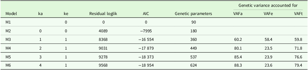
The first additive factor contained estimated loadings that all had the same sign (a 90/0 split of positive and negative values) so represents general yielding ability. The third and fourth additive factors and the single non-additive factor contained approximately equal mixtures of positive and negative values (splits of 38/52, 54/36 and 48/42, respectively) so are termed ‘bi-polar’ and thence represent contrasts between environments. The second additive factor is of particular interest. The majority of estimated loadings had the same sign (a 9/81 split of positive and negative) so the negative loadings will add to the general yielding ability but the contrast of positive and negative was found to have an important biological explanation that was revealed using iClass interaction plots (see later).
One of the aims of this analysis was the selection of L3 varieties tested in 2023 for ultimate commercial use. This requires consideration of the total of the additive and non-additive VE effects. Formation of iClasses for this purpose first requires ordering all five factors fitted in the model on the basis of the percentage of total genetic variance they account for. Using equation (11) and a value of $\overline a$
corresponding to the 125 L3 varieties, the percentage of total genetic variance accounted for by all five factors was 79.4 %, with the individual additive factors contributing 45.4, 20.7, 6.1 and 3.9 % and the non-additive factor contributing 3.3%. Thus, in this analysis, the ordering corresponded to additive factors one to four, followed by the single non-additive factor. The use of all five factors results in 13 iClasses, with labels and numbers of environments as given in the top half of Table 3. Also considered here is the use of only the four most important factors, which results in 8 iClasses as given in the bottom half of Table 3. The process of forming these iClasses is demonstrated in Table 4 which contains the rotated REML estimates of the loadings for the four additive factors and the REML estimates of the loadings for the single non-additive factor for a subset of 23 environments. The environments were chosen to cover all the iClasses formed using five factors, with two randomly chosen environments within each iClass (apart from the final three iClasses, each of which only contained one environment). This illustrates the patterns of the signs of the REML estimates of the loadings across factors which are used to define iClasses.
$\overline a$
corresponding to the 125 L3 varieties, the percentage of total genetic variance accounted for by all five factors was 79.4 %, with the individual additive factors contributing 45.4, 20.7, 6.1 and 3.9 % and the non-additive factor contributing 3.3%. Thus, in this analysis, the ordering corresponded to additive factors one to four, followed by the single non-additive factor. The use of all five factors results in 13 iClasses, with labels and numbers of environments as given in the top half of Table 3. Also considered here is the use of only the four most important factors, which results in 8 iClasses as given in the bottom half of Table 3. The process of forming these iClasses is demonstrated in Table 4 which contains the rotated REML estimates of the loadings for the four additive factors and the REML estimates of the loadings for the single non-additive factor for a subset of 23 environments. The environments were chosen to cover all the iClasses formed using five factors, with two randomly chosen environments within each iClass (apart from the final three iClasses, each of which only contained one environment). This illustrates the patterns of the signs of the REML estimates of the loadings across factors which are used to define iClasses.
Table 3. Number of environments in each interaction class for classes based on all 5 factors (top half of table) and classes based on the first 4 factors in order of percentage variance accounted for (bottom half of table)
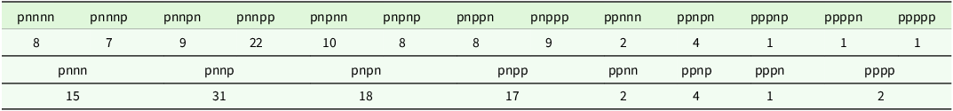
Table 4. Summary of information used to define interaction classes for a subset of 23 environments: rotated residual maximum likelihood estimates of loadings ( $ \times 1000$
) for each factor, ordered on variance accounted for (additive factors 1, 2, 3 and 4, non-additive factor 1); interaction classes based on all five factors and first four factors. The 23 environments cover all 13 interaction classes when five factors used, with two randomly chosen environments within each class (apart from the final three classes, each of which only contained one environment)
$ \times 1000$
) for each factor, ordered on variance accounted for (additive factors 1, 2, 3 and 4, non-additive factor 1); interaction classes based on all five factors and first four factors. The 23 environments cover all 13 interaction classes when five factors used, with two randomly chosen environments within each class (apart from the final three classes, each of which only contained one environment)
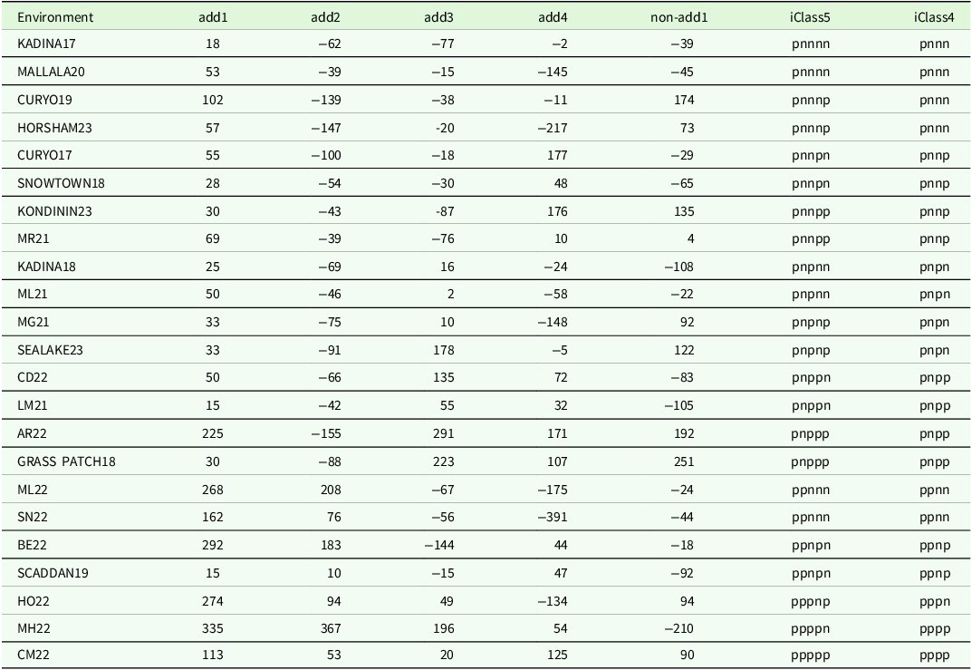
Recall that the estimated loadings for the second additive factor showed an uneven split of 9 positive values against 81 negatives. The estimated loadings for the first two additive factors are plotted against each other in Figure 2 and the 9 environments with positive loadings in the second factor have been labelled. The majority of these correspond to environments in 2022 which was an exceptionally wet year with conditions potentially leading to high disease pressure. The breeder was concerned that there may have been outbreaks of Botrytis Grey Mould (BGM) in these environments. To investigate this, an iClass interaction plot was constructed for three probe varieties, namely one variety (PBA BOLT) that is known to be susceptible to BGM and two varieties (ALB TERRIER and PBA JUMBO2) that are tolerant. The resultant plot in Figure 3 clearly demonstrates the existence of high levels of BGM in the iClasses corresponding to positive estimated loadings in the second additive factor. Henceforth, these iClasses will be termed ‘BGM iClasses’. The yield losses for the susceptible probe variety for the BGM iClasses as shown in Figure 3 were extreme (up to 3 t/ha). It was therefore recognised that the associated trials had essentially become disease tolerance trials and the breeder requested to exclude these results for the purposes of selection for general yielding ability. There was no need to re-do the analysis, however, as this can all be accommodated using iClasses.
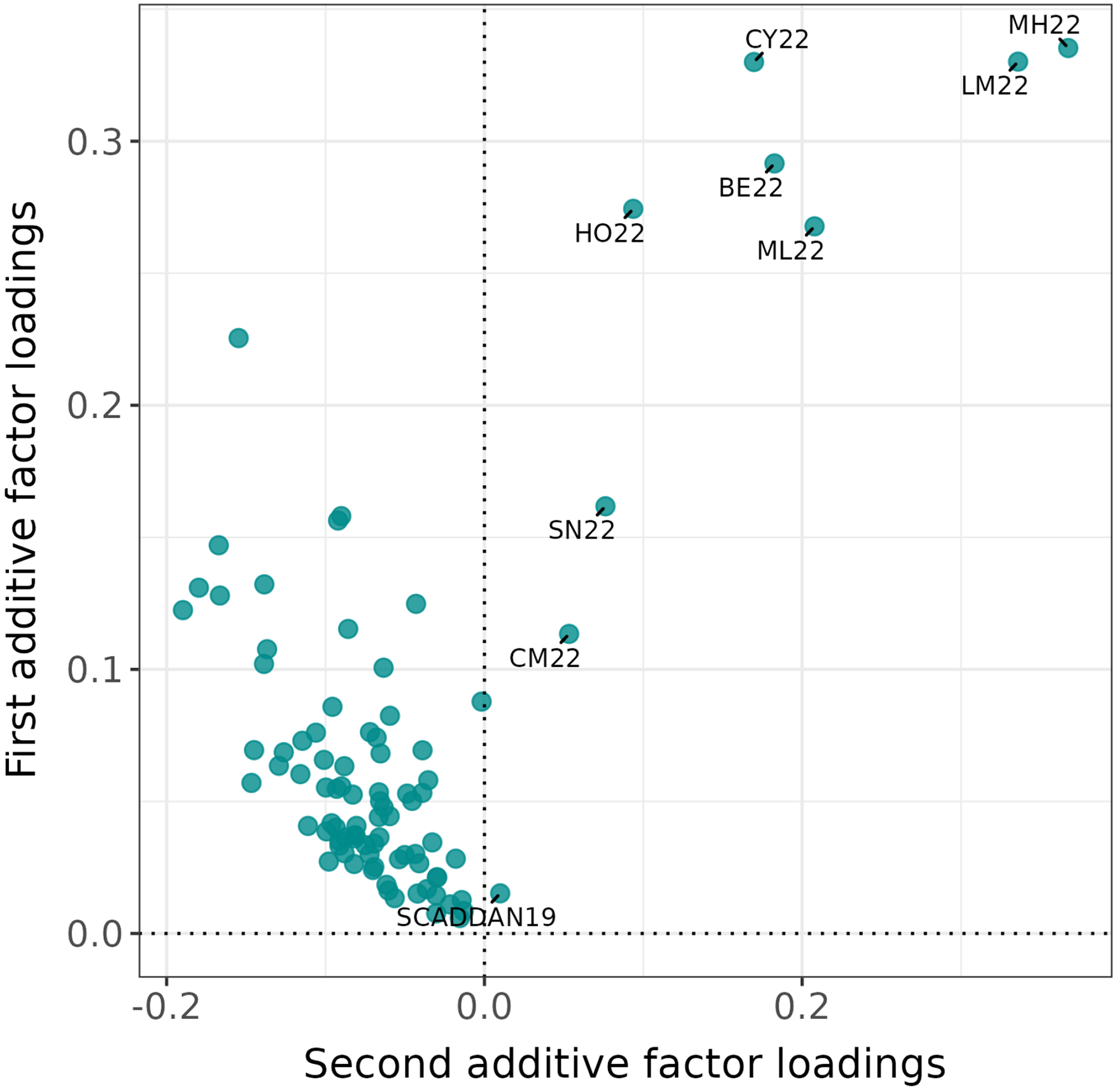
Figure 2. Rotated residual maximum likelihood estimates of loadings for first and second additive factors. Environments with positive estimated loadings in the second factor have been labelled.
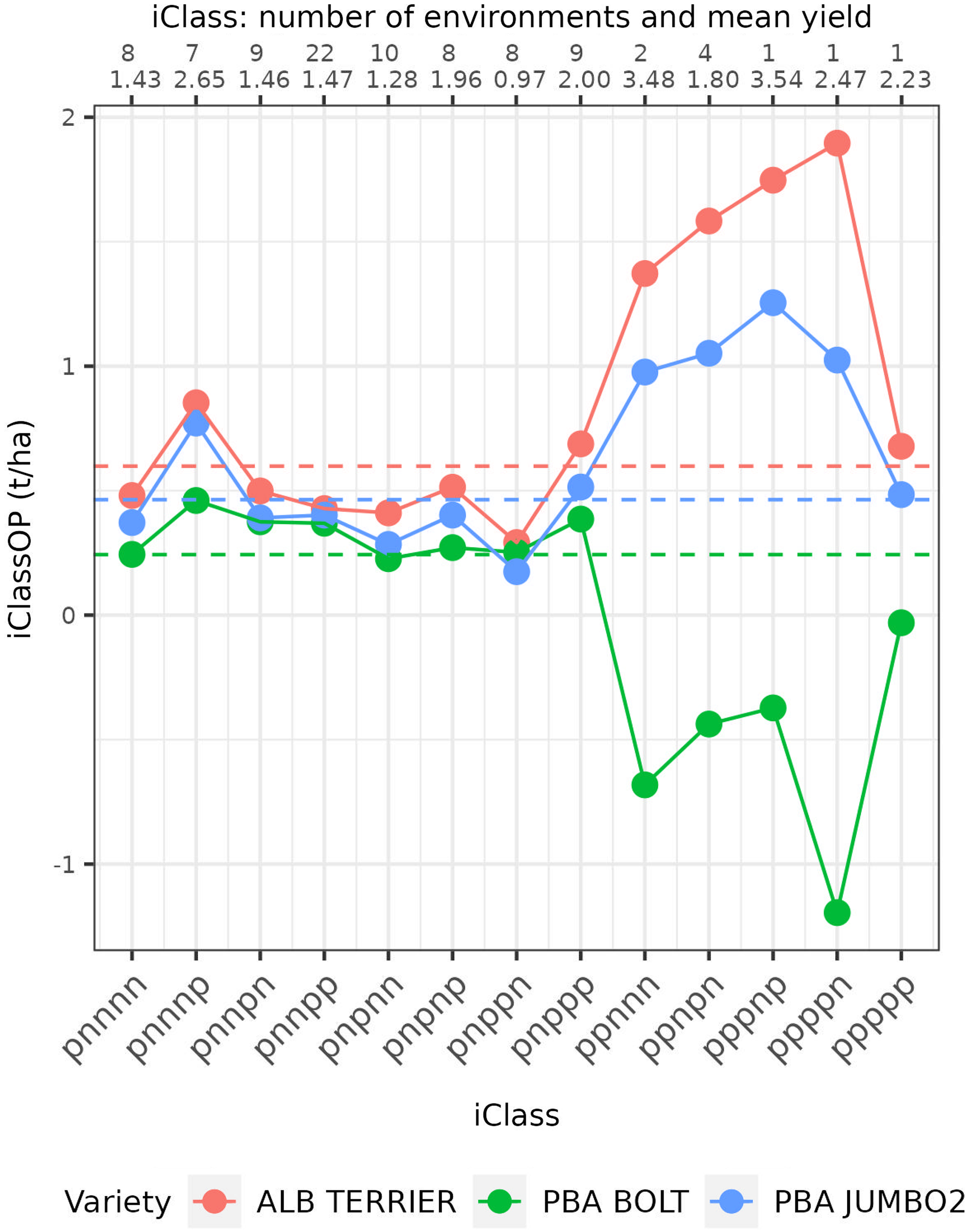
Figure 3. Plot of interaction class overall performance (t/ha) for three varieties that are probes for presence of the disease Botrytis Grey Mould. The variety PBA BOLT is a susceptible variety, whereas ALB TERRIER and PBA JUMBO2 are tolerant varieties. The number of environments in each iClass and their associated mean yield (t/ha) is given along the top axis. The dashed horizontal lines are the grand means of the common variety by environment effects across all environments for these varieties.
It is instructive to summarise the estimated genetic correlations between environments on an iClass basis. Given that variety iClassOP is based on the CVE effects, the estimated covariance matrix which excludes the contributions from the specific variances is considered. This can then be converted to a correlation matrix. Figure 4a contains a heatmap of these estimated correlations, summarised on the basis of interaction classes using five factors. The most obvious feature of this heatmap is the low genetic correlation between environments in BGM compared with non-BGM iClasses. The heatmap also shows there are strong correlations between all pairs of environments within an iClass. In contrast, the means of the pairwise estimated correlations involving environments in different iClasses are often quite low, indicating crossover interaction (even within the non-BGM iClasses). The analogous heatmap for iClasses based on the first four factors only is given in Figure 4b. One may be tempted to use these heatmaps to make the choice between using the first four or all five factors when forming iClasses. On this basis, it may appear that the use of interaction classes based on four factors might be reasonable, with the mean within iClass correlations ranging from 0.72 up to 0.82 (compared with 0.78 up to 0.88 using interaction classes based on five factors). However, it is important to recognise that genetic correlations as a measure of VEI are based on all the varieties in the dataset so may not be sufficiently specific for the varieties under consideration for selection. This issue is discussed further later.
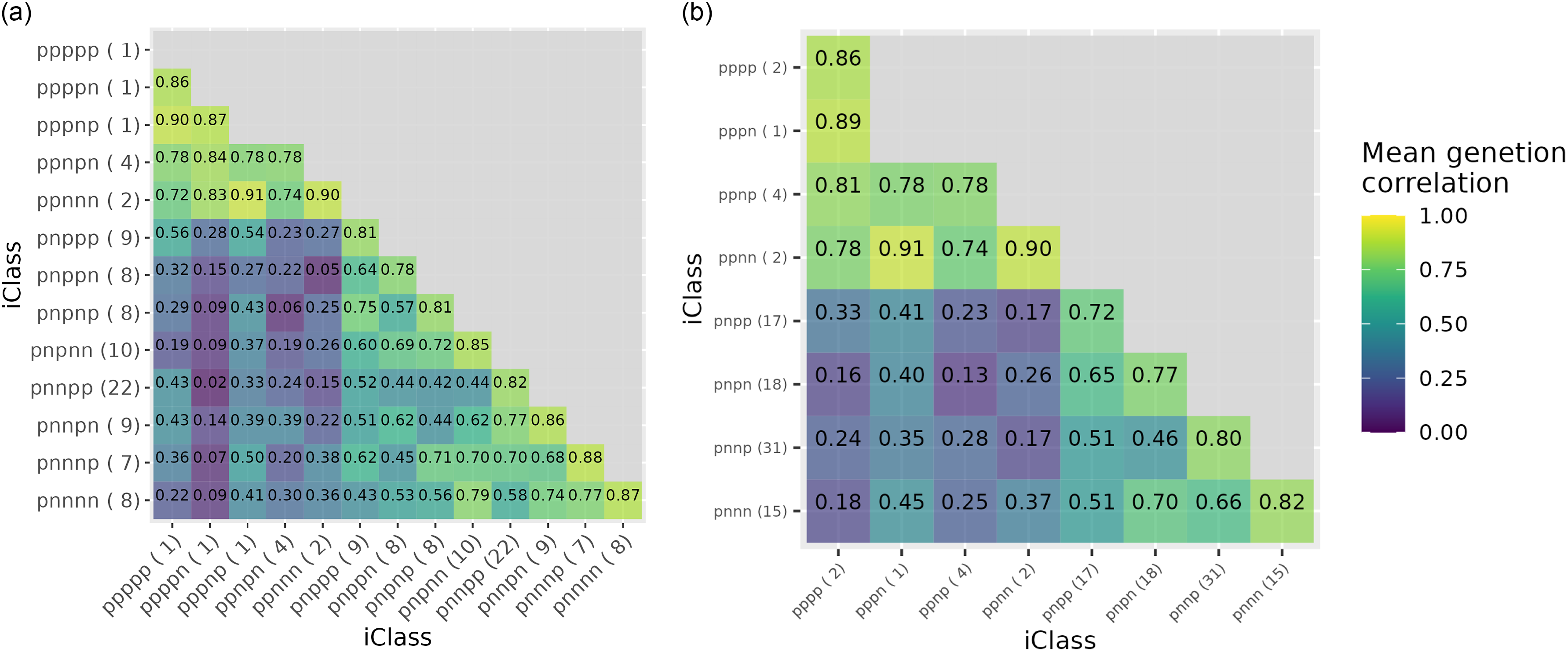
Figure 4. Estimated genetic correlations for total common variety by environment effects for all pairs of environments summarised on an interaction class basis for (a) classes based on all five factors and (b) classes based on first four factors. The value listed in each cell is the mean of all pairwise estimated correlations between environments in the interaction class. The interaction class labels include the associated numbers of environments in parentheses. The colour scale corresponds to the mean values.
In terms of variety selection, it is instructive to first consider the variety scores since these reflect their responses to the environmental covariates implied by the factor loadings. The aim of this section is selection amongst the 125 L3 varieties grown in 2023. Figure 5 plots the EBLUPs of the scores for the first additive factor against the remaining factors for these varieties. The varieties labelled in this figure correspond to six test lines (Test1 to Test6) and five commercial lines originating from this breeding programme. Of the latter, ALB TERRIER is the most recent variety. Each of the commercial varieties appeared in at least 75 environments in the dataset and in every year. The other labelled variety (ExtChk) is an important new commercial variety originating outside this breeding programme and whose parentage was unavailable for the purposes of this analysis. It was only grown in 14 environments in this dataset, all of which were in 2023. Given the nature of the environment loadings for the first two additive factors (as previously discussed) it is clear that varieties with large positive scores for the first factor and large negative scores for the second factor will likely yield well across a range of non-BGM environments. Therefore the majority of labelled test lines and the newer commercial variety look superior to the older commercial varieties. Test3 and Test4 look particularly promising and Test1 may also be but via a different mechanism. The large response of ExtChk to the last factor (the non-additive factor) is noteworthy and will be discussed later. Similarly, the behaviour of the two varieties ALB TERRIER and PBA HURRICANE XT (coloured red on the plots) will be explored later.
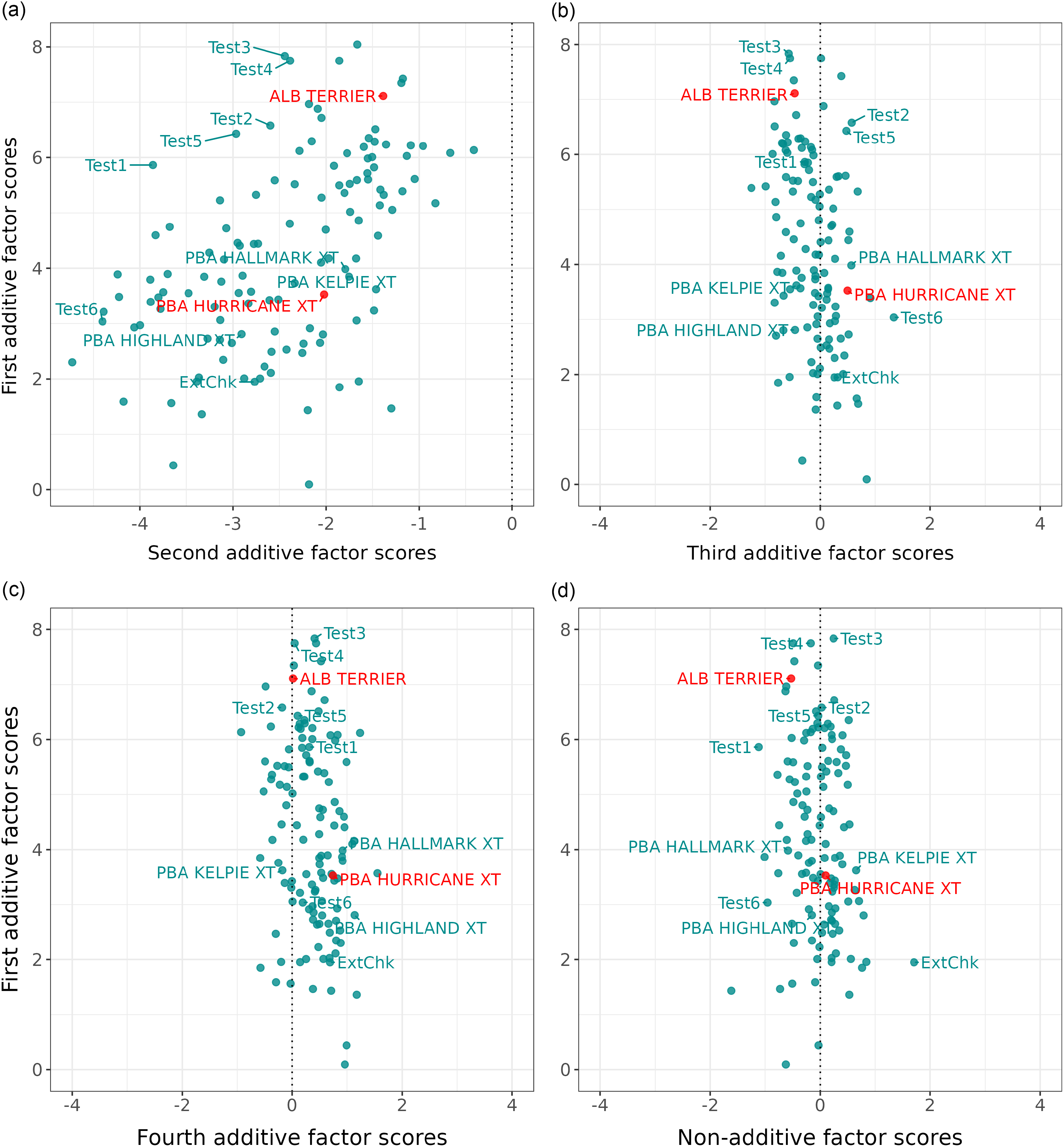
Figure 5. Empirical best linear unbiased predictions of additive factor scores for the 125 L3 varieties grown in 2023. Varieties of interest have been labelled with their names and two key varieties have been plotted in red. In each panel, the y-axis corresponds to the first factor and the x-axis to the second, third and fourth additive factors for (a), (b) and (c) and the non-additive factor for (d).
Whilst the score plots are extremely helpful in flagging varieties that have large responses to the factors, for the purposes of selection the totality of all these responses is required. Therefore the first step is to use the variety stability measure introduced in the Statistical Methods section. This is calculated for iClasses defined using all five factors and also using the first four only. It was of interest to examine stability for the non-BGM iClasses only, so the AOVs had either 8 levels for the treatment factor (when interaction classes based on five factors used) or 4 levels (when interaction classes based on four factors used). Figure 6 contains plots of the key information from the AOVs for each variety, namely the grand mean of the CVEs for non-BGM environments (on the y-axis), the square root of the between iClass mean square (on the x-axis) and the p-value for the ratio of the between to within iClass mean square (colour of the points). It is important to recognise that, because the CVEs are effects (not means), they are on the scale of the trait being analysed (here t/ha) but can be positive or negative. Thus, for example, a variety with a near zero CVE for an environment has an ‘average’ yield in that environment, whilst a variety with a large positive/negative CVE has above/below average yields for the environment. An analogous interpretation therefore follows through for both the grand means and iClassOP, each of which involves a simple arithmetic averaging across environments. Figure 6 only includes L3 varieties, which one would expect to have above-average yields relative to the entire population of varieties included in the MET. Thus all of the grand means are positive.
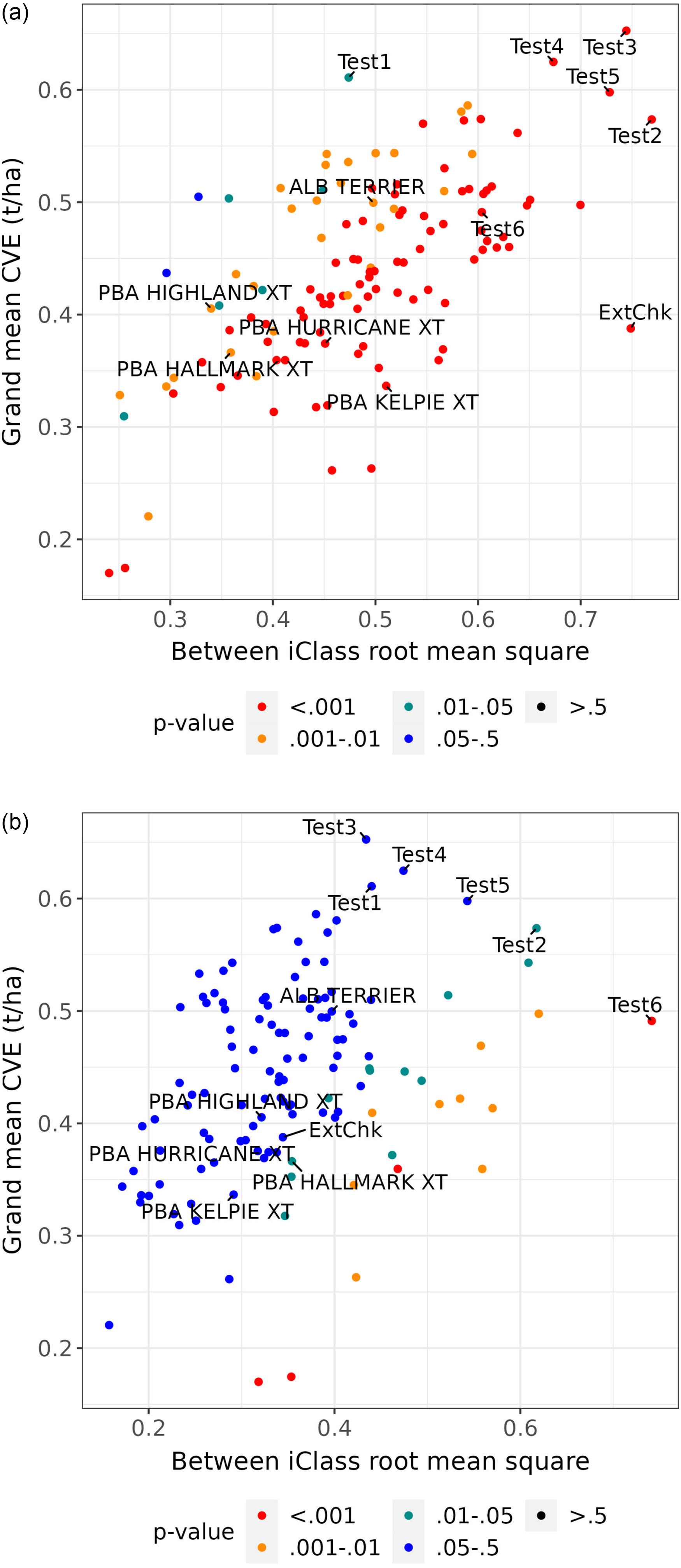
Figure 6. Stability across interaction classes (excluding those linked to the disease Botrytis Grey Mould) for the 125 L3 varieties grown in 2023: interaction classes defined using (a) all five factors and (b) first four factors. The y-axis in each plot is the grand mean of the common variety by environment effects (for each variety) across environments and the x-axis is the square root of the between interaction class mean square from the one-way analysis of variance on those effects. Points are coloured according to the p-value for the variance ratio from the analysis of variance. Varieties of interest have been labelled with their names.
A clear distinction between the two panels in Figure 6 is that when iClasses are defined using only the first four factors, many of the p-values are greater than 0.05 so that the within iClass mean square is arguably too large compared with the between iClass mean square. When all five factors are used, the majority (88) of p-values are less than 0.001. A full cross-tabulation of the p-values for iClasses defined using four or five factors is provided in Table 5. On the basis of this information it was decided to use iClasses based on all five factors to make selection decisions for the 125 L3 varieties. Note that, for other decisions, for example for the L0, L1 or L2 varieties, the associated stability plots may reveal a different story and it may be reasonable to use iClasses based on the first four factors alone. Clearly, this would simplify selection as it is then only necessary to examine four rather than eight iClasses. The key message is that it is not necessary to use the same sets of iClasses for all selection decisions. The stability plot in Figure 6a shows that most of the test lines are less stable than the commercial varieties. This is consistent with the change in the aims of the breeding programme which have moved away from breeding for broad adaptation to targeting specific environmental types. Also note that the grand means on the y-axis in the stability plot provide a naive measure of overall variety performance (in t/ha) across all environments considered (in this case the 81 non-BGM environments). Figure 6a shows that many of the test lines have higher grand means than the commercial varieties. However, it is not intended that these grand means be used as a trait for selection, as they ignore VEI, but rather to assist in choosing varieties to investigate thoroughly using interaction plots.
Table 5. Stability across interaction classes (excluding those linked to the disease Botrytis Grey Mould) for the 125 L3 varieties grown in 2023: p-values of variance ratios (ratio of between to within interaction class mean square) from analyses of variance tabulated for interaction classes defined using first four factors and all five factors
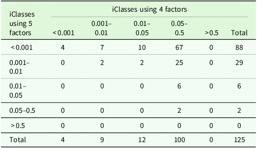
Both iClassOP and stability can be visually assessed in the interaction plots introduced in Smith et al. (Reference Smith, Norman, Kuchel and Cullis2021b) which display iClassOP for a chosen set of varieties across iClasses. Two such plots are given in Figure 7. As previously discussed, iClassOP for a variety can be positive or negative. All the values in Figure 7 are positive, indicating above-average yields for these varieties in all iClasses. As an aid to interpretation, the mean of the environment mean yields for each iClass is given on the top axis in the interaction plots. Thus, absolute yields for a variety within an iClass (within this MET) can be approximated by adding these means to iClassOP.
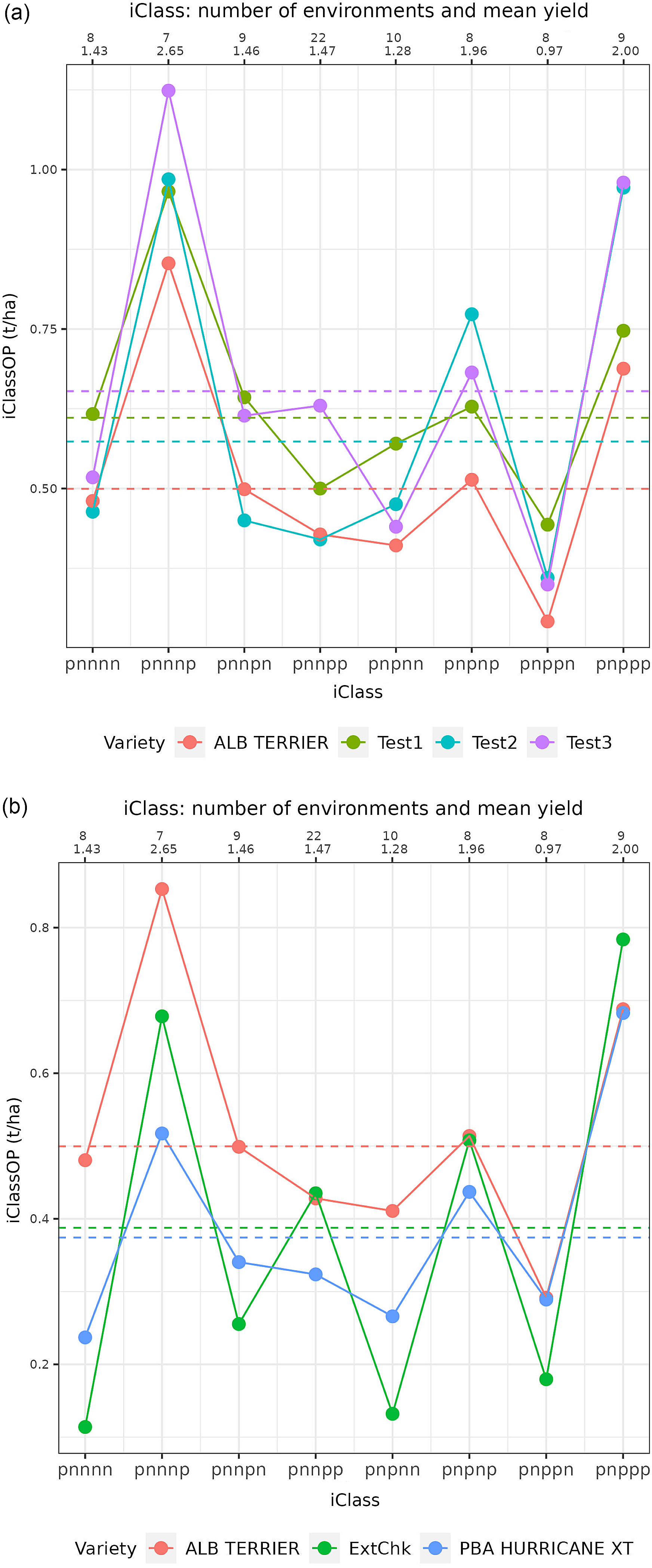
Figure 7. Plots of interaction class overall performance (t/ha) (excluding classes linked to the disease Botrytis Grey Mould) for (a) four varieties comprising ALB TERRIER and three test lines and (b) three varieties comprising ALB TERRIER and two other commercial varieties. The number of environments in each interaction class and their associated mean yield (t/ha) is given along the top axis. The dashed horizontal lines are the grand means of the common variety by environment effects for these varieties.
Figure 7a contains three test lines that had high grand means and varying levels of stability (as depicted in Figure 6a). The second panel contains the commercial variety PBA HURRICANE XT, which was released by the Agriculture Victoria lentil breeding programme in 2014, and the new external commercial variety which was released in 2023. To link the two panels, the commercial variety ALB TERRIER (released in 2024 by the Agriculture Victoria lentil breeding programme) is included on both. Figure 7a shows that Test1 and Test3 out-yield ALB TERRIER in all iClasses. Test3 yields particularly well, with an advantage of more than 0.2t/ha in three iClasses (pnnnp, pnnpp and pnppp). As expected from the stability plot, Test2 is quite unstable, ranking near the bottom of the four varieties in most iClasses, but ranking first or second in three iClasses (pnpnp, pnppp and pnnnp). Figure 7b shows that whilst the two varieties ExtChk and PBA HURRICANE XT had similar grand means, they exhibit substantial crossover VEI, with ExtChk ‘winning’ in all the iClasses with a ‘p’ as the final character, and PBA HURRICANE XT winning elsewhere. A more subtle, but equally important feature of Figure 7b is the comparison of ALB TERRIER and PBA HURRICANE XT. To aid in interpretation, the actual iClassOP values for these varieties are provided in Table 6, together with the differences. Also given are the factor scores. Recall that the factors, when ordered as in this table, have decreasing variance accounted for so have decreasing influence on CVEs and thence iClassOP. All iClasses under consideration have the same first two characters, ‘pn’ so that varieties with large positive scores for the first additive factor and, to a lesser extent, large negative scores for the second factor, will yield well across most iClasses. Thus it would be expected that ALB TERRIER, with a much higher score than PBA HURRICANE XT for the first factor would have superior performance across most iClasses. This is borne out on Figure 7b, but it is clear that the magnitude of the superiority of ALB TERRIER changes dramatically across iClasses, with essentially no difference between the two varieties in the two iClasses on the far right of the graph. This is due mainly to the differences in scores for additive factors three and four, and to a lesser extent the non-additive factor (also see Figure 5 in which PBA HURRICANE XT appears to the right of ALB TERRIER on panels (b), (c) and (d)). The differences in Table 6 and the score plots reveal that PBA HURRICANE XT would be boosted relative to ALB TERRIER for iClasses with a ‘p’ as the third character, and even more so for iClasses with a ‘p’ as third and fourth (and finally fifth) character. Thus moving from left to right on Figure 7b, the factor scores suggest it would be expected for ALB TERRIER to out-yield PBA HURRICANE XT by a substantial amount in iClasses pnnnn and pnnnp, to a lesser extent in iClasses pnnpn and pnnpp and also pnpnn and pnpnp. Finally, in pnppn and pnppp, PBA HURRICANE XT has ‘caught up’. This example clearly shows how iClassOP encapsulates and combines all of the information in the factor scores.
Table 6. Interaction class overall performance (t/ha) and factor scores for ALB TERRIER and PBA HURRICANE XT. Also given are the differences between the two varieties (ALB TERRIER and PBA HURRICANE XT for interaction class overall performance and the reverse order for factor scores.)
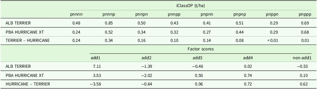
Discussion
Smith et al. (Reference Smith, Norman, Kuchel and Cullis2021b) addressed the key issue of variety selection in the presence of VEI within the framework of a FALMM. They developed their ‘iClass’ methodology for models in which the genetic effects for different varieties were assumed independent. In the current paper this has been extended for models that incorporate information on the genetic relatedness of varieties. Thus the variety effects in different environments are partitioned into additive and non-additive, with a separate FA model for each set of effects. This class of models is recommended, and widely used in Australia, for annual selection decisions by plant breeding programmes. In the example presented in this paper, genetic relatedness was included in the LMM via pedigree information. The resultant improvement in the goodness of fit of the model, as assessed via the residual log-likelihood, was undeniably substantial. Similar, or possibly greater gains, may result with the use of genomic information. Either way, the key message is the importance of using genetic relatedness to improve the accuracy of variety selection. An associated issue is that when an appropriate MET dataset is used for analysis (see later), the resultant incompleteness in terms of varieties being grown in the trials necessitates the use of genetic relatedness to provide links between environments.
As in Smith et al. (Reference Smith, Norman, Kuchel and Cullis2021b) it is stressed here that although the iClass approach involves the formation of groups of environments for the purpose of obtaining average (or overall) variety effects, it is not a clustering of environments based on genetic correlations. Given that genetic correlations reflect relationships between environments based on all varieties, it is not uncommon for a clustering on this basis to mask individual variety patterns of VEI. Instead of focussing on the environments, the iClass approach focusses attention on the actual subject of the selection decisions, namely the varieties. Specifically, the iClasses are formed in such a way that they discriminate varieties with different patterns of VEI. This is achieved using the fact that when a factor is bi-polar, there is crossover interaction of varieties (for the fitted values for that factor) between the environments with positive estimated loadings compared with negative. Hence the formation of iClasses using a concatenation across factors of the signs of the estimated loadings for each environment.
An issue that is often raised is whether iClasses can be ascribed a meaningful interpretation. Clearly, the labelling protocol is designed to illustrate the contrasting groups of environments (positive versus negative estimated loadings) for each factor used in forming the iClasses. In the authors’ experience, breeders have often been able to link iClasses to key environmental variables such as disease prevalence and growing conditions. Current work focusses on a formal statistical approach to achieve this, with the ultimate aim of being able to assign a meaningful environmental label to each iClass. In the interim, the complementary approach based on probe genotypes (see Cooper and Fox, Reference Cooper, Fox, Cooper and Hammer1996, for example) has been used successfully for iClass interpretation. This approach can be regarded as a bioassay in which varieties with known reactions to environmental factors are used to characterise the environments in a MET. A key example in the current paper was the use of probe varieties to detect the existence of the disease BGM. Three varieties (one susceptible and two tolerant) were visualised in an iClass interaction plot, and this led to the conclusion that iClasses with a ‘p’ as the second character in their label comprised environments with high levels of BGM. These iClasses were therefore termed ‘BGM iClasses’ and the breeder consequently requested to exclude them when making selection decisions for grain yield as they provided more of an assessment of tolerance rather than general yielding ability.
As alluded to above, another key requirement for variety selection is the use of a suitable MET dataset. As discussed in Smith et al. (Reference Smith, Ganesalingam, Lisle, Kadkol, Hobson and Cullis2021a) the dataset should include all trials that provide data on the selection history for the varieties under consideration for selection. This typically leads to incomplete (not all varieties in all trials) datasets with large numbers of environments that span multiple years and stages of selection. In the example presented in this paper, the MET dataset comprised 90 environments and spanned 7 years. The analysis of these data, as conducted in this paper, would have facilitated selection for four stages of selection (L0, L1, L2 and L3) for varieties grown in 2023. In the current paper, for reasons of brevity and clarity, only the L3 selection decisions were fully explored. The key point here is that it is unsatisfactory to ‘slice and dice’ datasets to achieve, for example, a complete dataset, or to reduce the size in order to avoid computational difficulties associated with statistical software. The latter may include both memory and time limitations. Linked to this issue is the preponderance in the literature of two- (or three-) stage analyses for MET data. It has long been established that the one-stage analysis, as presented in this paper, is superior, irrespective of any weighting scheme that may be proposed (Gogel, Reference Gogel1997; Gogel et al., Reference Gogel, Smith and Cullis2018). Two-stage approaches were historically necessary when individual plot data was not stored electronically and when statistical software and/or computer hardware was inadequate.
As in Smith et al. (Reference Smith, Norman, Kuchel and Cullis2021b), the approach in this paper forms groups of environments, called iClasses, on the basis of which meaningful summaries of variety performance for the trait of interest (assumed here to be yield) can be obtained. In Smith et al. (Reference Smith, Norman, Kuchel and Cullis2021b) the summary measure provided was overall yield level (iClassOP) for each variety in each iClass. The iClass interaction plot was introduced as a means of displaying this information, thence allowing a comparison of varieties in terms of their performance across iClasses. In the current paper, a measure of stability of variety performance across iClasses has been proposed. This quantifies the fluctuations in iClassOP as visualised on the interaction plot. Stability was shown to be useful in its own right as a means for choosing varieties of interest to explore in detail using an interaction plot. Additionally, it was helpful for assessing the appropriateness of using only a subset of the fitted factors (the most important factors) to define iClasses. This was found to be particularly important for the motivating example.
Conclusion
Variety selection in a plant breeding programme requires three key statistical inputs, namely
-
a MET dataset that comprises the entire selection history (or as much as possible) of the current cohort of varieties
-
a one-stage statistical analysis that accommodates incomplete data, includes information on genetic relatedness and encapsulates complex patterns of VEI
-
meaningful summaries of variety predictions from the analysis
The current paper addresses the final component within the framework of datasets and a method of analysis (the FALMM) that satisfy the first two components. The summaries relate to groups of environments called iClasses, the definitions of which are derived from the core parameters in the FALMM, namely the factor loadings for environments. The summaries of variety performance across iClasses provide growers and stakeholders not only with information about ‘what wins where’, but also about the actual yield advantage (in t/ha, for example) of the winners. This can have significant impact on the economics of variety choice.
Acknowledgement
ABS and BC would like to thank the plant breeders and plant industry professionals with whom they have had numerous discussions leading to refinements in the methodology and its application. The list of personnel includes (in no particular order) Garry Rosewarne and Babu Pandey (Agriculture Victoria); Colin Cavanagh (BASF); Kristy Hobson (Chickpea Breeding Australia); Aanandini Ganesalingam, Dan Mullen, David Tabah and David Moody (InterGrain Pty Ltd); Haydn Kuchel and Adam Norman (Australian Grain Technologies); Trevor Doerksen (Forest Genetics, British Columbia), Justin Kudnig and Willow Liddle (Advanta Seeds Pty Ltd). We thank these and other collaborators for their continued support.
Supplementary material
The supplementary material for this article can be found at https://doi.org/10.1017/S0021859625000085
Data availability statement
The data analysed in this paper cannot be made publicly available for commercial reasons associated with Agriculture Victoria’s lentil breeding programme.
Funding statement
Agriculture Victoria’s lentil breeding programme is jointly funded by Agriculture Victoria Research and Grains Research and Development Corporation (GRDC).
Competing interests
The authors declare that there are no competing interests.
Ethical standards
Not applicable.
Software availability statement
The DWReml and pedicure packages used in this paper were developed by David Butler and Brian Cullis. Beta versions are freely available from Brian Cullis (bcullis@uow.edu.au) on request.
Appendix Percentage variances associated with total VE effects
It is often of interest to compute various quantities as percentages of total (additive plus non-additive) genetic variance. For example, the additive genetic variance for an environment as a percentage of total genetic variance for the environment and the variance accounted for by individual terms in the factor analytic models as a percentage of the total genetic variance.
In order to compute these percentages, it is instructive to consider the variance structure for individual varieties so first define ${{\boldsymbol u}_g}_{\left( i \right)} = {({u_{{g_{i1}}}},{u_{{g_{i2}}}}, \ldots, {u_{{g_{ip}}}})^ \top }$
to be the
${{\boldsymbol u}_g}_{\left( i \right)} = {({u_{{g_{i1}}}},{u_{{g_{i2}}}}, \ldots, {u_{{g_{ip}}}})^ \top }$
to be the $p \times 1$
vector of total VE effects for variety
$p \times 1$
vector of total VE effects for variety $i$
. Then note that
$i$
. Then note that
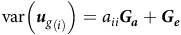 $${\rm{var}}\left( {{{\boldsymbol u}_g}_{\left( i \right)}} \right) = {a_{ii}}{\boldsymbol {G_a}} + {\boldsymbol {G_e}}$$
where ${a_{ii}}$
is the
${a_{ii}}$
is the $i^{th}$
diagonal element of the relationship matrix (either NRM or GRM). Equation (A1) shows that expressions of quantities as a percentage of total genetic variance will differ depending on
$i^{th}$
diagonal element of the relationship matrix (either NRM or GRM). Equation (A1) shows that expressions of quantities as a percentage of total genetic variance will differ depending on ${a_{ii}}$
so that specific values of interest must be chosen. Often, the mean of the diagonal elements of the relationship matrix is used, and this will be denoted by
${a_{ii}}$
so that specific values of interest must be chosen. Often, the mean of the diagonal elements of the relationship matrix is used, and this will be denoted by $\overline a$
. Then, for example, the percentage of additive variance for environment
$\overline a$
. Then, for example, the percentage of additive variance for environment $j$
can be computed as
$j$
can be computed as
 $$100 \times {{\overline a{g_{{a_{jj}}}}} \over {\overline a{g_{{a_{jj}}}} + {g_{{e_{jj}}}}}}$$
where ${g_{{a_{jj}}}}$
and
${g_{{a_{jj}}}}$
and ${g_{{e_{jj}}}}$
are the
${g_{{e_{jj}}}}$
are the $j^{th}$
diagonal elements of
$j^{th}$
diagonal elements of ${\boldsymbol {G_a}}$
and
${\boldsymbol {G_a}}$
and ${\boldsymbol {G_e}},$
respectively. Note that as an alternative to using an overall
${\boldsymbol {G_e}},$
respectively. Note that as an alternative to using an overall $\bar a$
value, a separate value for each environment could be used. Thus,
$\bar a$
value, a separate value for each environment could be used. Thus, $\overline a$
in equation (A2) could be replaced by
$\overline a$
in equation (A2) could be replaced by ${\overline a_j}$
, where this is the mean of the diagonal elements of the relationship matrix corresponding to those varieties grown in environment
${\overline a_j}$
, where this is the mean of the diagonal elements of the relationship matrix corresponding to those varieties grown in environment $j$
.
$j$
.


 Open access