2 Preliminaries and main result

2.1 Preliminaries

Suppose that $\mathfrak {M}$ is a compact metric space, $\sigma :\mathfrak {M}\to \mathfrak {M}$ is a homeomorphism, and $\mu $ is an ergodic invariant Borel probability measure supported on $\mathfrak {M}$ . Assume also that we are given a continuous map $g_{\cdot }:\mathfrak {M}\to {\operatorname {\mathrm {Homeo}}}^+(S^1)$ , where by $\operatorname {\mathrm {Homeo}}^+(S^1)$ , we denote the space of orientation-preserving homeomorphisms of the circle, where $S^1=\mathbb {R}/\mathbb {Z}$ denotes the circle. Then, one can consider an associated skew product

$$ \begin{align*} F:(\omega, x)\mapsto (\sigma \omega, g_{\omega} (x)). \end{align*} $$

Next, let us choose for every $\omega \in \mathfrak {M}$ a lift $\tilde g_{\omega }:\mathbb {R}\to \mathbb {R}$ of the map $g_{\omega }\in Homeo^+(S^1)$ ,

$$ \begin{align*} g_{\omega}(\pi(x))=\pi(\tilde g_{\omega}(x)), \end{align*} $$

where $\pi :\mathbb {R}^1\to S^1$ is a natural covering map, in such a way that $\{\tilde g_{\omega }(0)\}$ is a bounded measurable (in $\omega $ ) function (e.g. one can require $g_{\omega }(0)\in [0,1)$ for all $\omega \in \mathfrak {M}$ ). We then can consider the associated lift of the skew product:

(1) $$ \begin{align} \tilde F:(\omega, x)\mapsto (\sigma \omega, \tilde g_{\omega} (x)). \end{align} $$

Finally, let $G_{m,\omega }$ and $\tilde G_{m,\omega }$ be the length m fiberwise compositions associated to these skew products:

$$ \begin{align*} F^m (\omega,x)=(\sigma^m \omega, G_{m,\omega}(x)), \quad \tilde F^m (\omega,x)=(\sigma^m \omega, \tilde G_{m,\omega}(x)), \end{align*} $$

so that for $m>0$ , we have

$$ \begin{align*} \tilde G_{m,\omega}=\tilde g_{\sigma^{m-1}\omega}\circ \cdots \circ \tilde g_{\sigma\omega}\circ\tilde g_{\omega}. \end{align*} $$

The following statement is well known (e.g. see [Reference HermanHer, §5], [Reference RuelleR], or [Reference Gorodetski and KleptsynGK, Appendix A]).

Proposition 2.1. There exists a number $\rho \in \mathbb {R}$ such that for $\mu $ -almost every (a.e.) $\omega \in \mathfrak {M}$ and every $x\in \mathbb {R}$ , the limit

(2) $$ \begin{align} \lim_{n\to \infty}\frac{1}{n} (\tilde G_{n,\omega} (x)-x) \end{align} $$

exists and is equal to $\rho $ .

The number $\rho $ from Proposition 2.1 is called the rotation number. Notice that the rotation number $\rho $ depends on the choice of lifts $\tilde g_{\omega }$ .

Remark 2.2. It can happen that the lifts $\{\tilde g_{\omega }\}$ cannot be taken continuous in $\omega $ . At the same time, in the case when $\{g_{\omega }\}$ are projectivizations of the transfer matrices of a Schrödinger cocycle defined by a continuous potential, the lifts $\{\tilde g_{\omega }\}$ can always be chosen continuously in $\omega $ (since any Schrödinger cocycle is homotopic to a constant one).

Remark 2.3. Some of the assumptions in Proposition 2.1 can be essentially relaxed. For example, one can start with a probability space $(\mathfrak {M}, \mu )$ and a measure-preserving transformation $\sigma $ instead on a measure-preserving homeomorphism of a compact metric space. To keep the presentation more transparent, we are not trying to give the statements in the most general form.

Let us now consider the dependence of the rotation number on a parameter. Namely, assume now that we are given a continuous family $g_{\cdot ,\cdot }: J\times \mathfrak {M} \to \operatorname {\mathrm {Homeo}}_+(S^1)$ of maps as above; here, $J\subseteq \mathbb {R}^1$ is a closed interval of parameters. Then, we can consider their lifts $\tilde {g}_{a,\omega }:{\mathbb R}\to {\mathbb R}$ to be chosen continuously in parameter $a\in J$ . The corresponding skew products $F_a$ and $\tilde F_a$ as well as the fiberwise compositions $G_{n,a,\omega }$ and $\tilde G_{n,a,\omega }$ then can be defined in the same way as before.

An important note is that the increments of the images ${\tilde {G}}_{n,a',\omega }(x)-{\tilde {G}}_{n,a,\omega }(x)$ do not depend on a particular choice of lifts $\tilde {g}_{a,\omega }$ . Moreover, this increment is continuous in $\omega $ and x (and in fact is a well-defined function of the point x on the circle, not only on the real line). Also, dividing by n and passing to the limit, one gets that the difference of the corresponding rotation numbers $\rho (a')-\rho (a)$ does not depend on the choice of lifts $\tilde {g}_{a,\omega }$ , thus getting the following important note.

Remark 2.4. Even though the rotation number $\rho $ depends on a particular choice of the lifts $\tilde {g}_{a,\omega }$ , the differences of rotation numbers $\rho (a')-\rho (a)$ do not. In particular, different choice of lifts $\tilde g_{a, \omega }$ leads to a shift of the rotation number $\rho (a)$ by a constant, and intervals in the space of parameters where $\rho $ is constant are independent of the choice of the lifts.

2.3 Proof of the main result

Proof. Fix $a', a\in J$ , and set $\delta =C|a'-a|$ . It suffices to show that equation (3) holds for all $a, a'\in J$ that are sufficiently close to each other. Therefore, without loss of generality, we can assume

(4) $$ \begin{align} \delta<0.1\quad \text{and}\quad |a'-a|<C. \end{align} $$

Take any initial point $x_0=x_0'\in {\mathbb R}$ , for instance, $x_0=x_0'=0$ . Consider the sequences of its iterates associated to some $\omega \in \Omega $ and two different parameter values $a,a'\in J$ , for $n\ge 1$ ,

$$ \begin{align*} x_{n}&={\tilde{G}}_{n, a, \omega}(x_0)=\tilde{g}_{a, \sigma^{n-1}(\omega)}(x_{n-1}),\\ x^{\prime}_{n}&={\tilde{G}}_{n, a', \omega}(x_0)=\tilde{g}_{a', \sigma^{n-1}(\omega)}(x^{\prime}_{n-1}) \end{align*} $$

(to simplify the notation, we do not indicate the dependence on $\omega $ explicitly).

Then, for $\mu $ -a.e. $\omega \in \mathfrak {M}$ , we have

(5) $$ \begin{align} \rho(a')-\rho(a)=\lim_{n\to \infty}\frac{1}{n}(x^{\prime}_n - x_n). \end{align} $$

To prove equation (3), we can assume without loss of generality that $\rho (a')>\rho (a)$ , as the other case differs only by interchanging a and $a'$ . The following lemma compares the evolution of distances between the two orbits (considered for the same $\omega $ ).

Lemma 2.8. For any $n=1,2,\ldots $ and any integer j, the following holds:

(6) $$ \begin{align} x^{\prime}_n-x_n - j \le \delta + M_{\sigma^{n-1}\omega} \cdot \max (0,x^{\prime}_{n-1}-x_{n-1} - j). \end{align} $$

Proof. Consider the point $y:=\tilde {g}_{a, \sigma ^{n-1}(\omega )}(x^{\prime }_{n-1})$ . Applying the Lagrange theorem, due to the choice of C, we then have

$$ \begin{align*} |x^{\prime}_n-y| = | \tilde{g}_{a', \sigma^{n-1}(\omega)}(x^{\prime}_{n-1}) - \tilde{g}_{a, \sigma^{n-1}(\omega)}(x^{\prime}_{n-1})| \le C \cdot |a'-a| =\delta. \end{align*} $$

Thus, to establish equation (6), it suffices to show that

(7) $$ \begin{align} y-x_n - j \le M_{\sigma^{n-1}\omega} \cdot \max (0,x^{\prime}_{n-1}-x_{n-1} - j). \end{align} $$

However, we have

$$ \begin{align*} y-x_n - j&= \tilde{g}_{a, \sigma^{n-1}(\omega)}(x^{\prime}_{n-1}) - \tilde{g}_{a, \sigma^{n-1}(\omega)}(x_{n-1}) - j \\ &= \tilde{g}_{a, \sigma^{n-1}(\omega)}(x^{\prime}_{n-1}-j) - \tilde{g}_{a, \sigma^{n-1}(\omega)}(x_{n-1}), \end{align*} $$

where the second equality uses the fact that $\tilde {g}_{a, \sigma ^{n-1}(\omega )}$ commutes with integer shifts (see Figure 1).

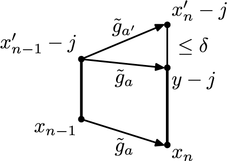
Figure 1 Action of maps $\tilde {g}_{a, \sigma ^{n-1}(\omega )}$ and $\tilde {g}_{a', \sigma ^{n-1}(\omega )}$ .

If $x^{\prime }_{n-1}-x_{n-1} - j\le 0$ , then due to the monotonicity of $\tilde {g}_{a, \sigma ^{n-1}(\omega )}$ ,

$$ \begin{align*} y-j = \tilde{g}_{a, \sigma^{n-1}(\omega)}(x^{\prime}_{n-1}-j) \le \tilde{g}_{a, \sigma^{n-1}(\omega)}(x_{n-1}) = x_n, \end{align*} $$

and equation (7) holds. Otherwise, we again apply the Lagrange theorem:

$$ \begin{align*} y-x_n - j = \frac{d\tilde{g}_{a, \sigma^{n-1}(\omega)}}{dx} \bigg|_{\xi} \cdot ((x_{n-1}'-j) - x_{n-1}) \le M_{\sigma^{n-1}\omega} \cdot \max (0,x^{\prime}_{n-1}-x_{n-1} - j), \end{align*} $$

where $\xi \in \mathbb {R}$ is a point between $x_{n-1}'-j$ and $x_{n-1}$ . This completes the proof of Lemma 2.8.

The conclusion of this lemma immediately implies the following corollary.

Corollary 2.9. Denote $d_{n,j}:= \delta + \max (0,x^{\prime }_n-x_n-j)$ . Then,

$$ \begin{align*} d_{n,j} \le M_{\sigma^{n-1}\omega} \cdot d_{n-1,j}. \end{align*} $$

Consider now the sequence of the first moments $n_j$ when the orbit associated to $a'$ goes j full turns ahead of the one associated to a:

$$ \begin{align*} n_j=\min\{n \ge 0 \mid \ x^{\prime}_{n}\ge x_{n}+j\}. \end{align*} $$

This sequence is well defined for $\mu $ -a.e. $\omega \in \mathfrak {M}$ due to equation (5) and the assumption $\rho (a')>\rho (a)$ . We have the following lemma.

Lemma 2.10. For every $j\ge 0$ ,

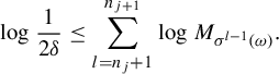$$ \begin{align*} \log \frac{1}{2\delta} \le \sum_{l=n_{j}+1}^{n_{j+1}}\log M_{\sigma^{l-1}(\omega)}. \end{align*} $$

Proof. Applying Corollary 2.9, we get

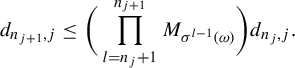$$ \begin{align*} d_{n_{j+1},j} \le \bigg(\prod_{l=n_{j}+1}^{n_{j+1}} M_{\sigma^{l-1}(\omega)} \bigg) d_{n_j,j}. \end{align*} $$

However, $d_{n_{j+1},j}\ge 1$ by definition, while $d_{n_j,j}\le 2\delta $ due to Lemma 2.8. Taking the logarithm concludes the proof.

We are now ready to complete the proof of Theorem 2.5. Namely, for every $\mu $ -regular point $\omega \in \mathfrak {M}$ , we have

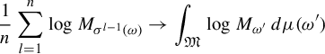$$ \begin{align*} \frac{1}{n}\sum_{l=1}^n \log M_{\sigma^{l-1}(\omega)}\to \int_{\mathfrak{M}}\log M_{\omega'}\,d\mu(\omega') \end{align*} $$

as $n\to \infty $ . In particular, for all sufficiently large values of $n\in \mathbb {N}$ , we have

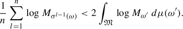$$ \begin{align*} \frac{1}{n}\sum_{l=1}^n \log M_{\sigma^{l-1}(\omega)} < 2 \int_{\mathfrak{M}}\log M_{\omega'}\,d\mu(\omega'). \end{align*} $$

Hence, for all large enough $j\in \mathbb {N}$ ,

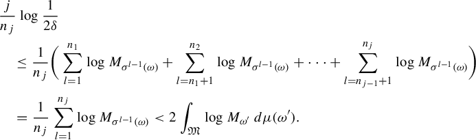$$ \begin{align*} &\frac{j}{n_j}\log \frac{1}{2\delta} \\ &\quad \le \frac{1}{n_j}\bigg(\sum_{l=1}^{n_1} \log M_{\sigma^{l-1}(\omega)}+\sum_{l=n_1+1}^{n_2} \log M_{\sigma^{l-1}(\omega)}+\cdots+ \sum_{l=n_{j-1}+1}^{n_j} \log M_{\sigma^{l-1}(\omega)}\bigg)\\ &\quad =\frac{1}{n_j}\sum_{l=1}^{n_j} \log M_{\sigma^{l-1}(\omega)}<2\int_{\mathfrak{M}}\log M_{\omega'}\,d\mu(\omega'). \end{align*} $$

By definition of $\{n_j\}$ , we have $ j\le |x^{\prime }_{n_j}- x_{n_j}|\le j+1, $ and hence

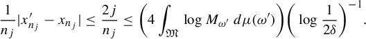$$ \begin{align*} \frac{1}{n_j}|x_{n_j}'- x_{n_j}|\le \frac{2j}{n_j}\le \bigg(4\int_{\mathfrak{M}}\log M_{\omega'}\,d\mu(\omega')\bigg)\bigg(\log \frac{1}{2\delta}\bigg )^{-1}. \end{align*} $$

Taking into account equation (5), this implies that

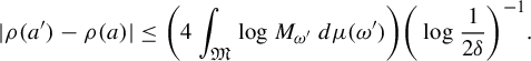(8) $$ \begin{align} |\rho(a')-\rho(a)|\le \bigg(4\int_{\mathfrak{M}}\log M_{\omega'}\,d\mu(\omega')\bigg)\bigg(\log \frac{1}{2\delta} \bigg)^{-1}. \end{align} $$

Finally,

$$ \begin{align*} \log \frac{1}{2\delta} = \log |a-a'|^{-1} - \log 2C> \frac{1}{2} \log |a-a'|^{-1} \end{align*} $$

once $|a-a'|<e^{-4C}$ ; hence, for such $a,a'$ , the estimatein equation (8) implies

$$ \begin{align*} |\rho(a')-\rho(a)| \le R \, (\log|a'-a|^{-1})^{-1}, \end{align*} $$

where $R=8\int _{\mathfrak {M}}\log M_{\omega '}\,d\mu (\omega ')$ .

Due to compactness of J, the same inequality holds also if we remove the assumption of $a,a'$ being sufficiently close, possibly with a larger value of constant R. This completes the proof of Theorem 2.5.

3 The Craig–Simon theorem on log-Hölder regularity of the IDS

In this section, we explain that an application of Theorem 2.5 to the Schrödinger cocycle of the corresponding 1D ergodic Schrödinger operator immediately implies that the integrated density of states must be log-Hölder regular; therefore, providing a purely dynamical proof of the classical Craig–Simon result in spectral theory [Reference Craig and SimonCS2, Theorem 5.2]. For the modern presentation of all the necessary background in the theory of ergodic Schrödinger operators, see [Reference Damanik and FillmanDF1, Reference Damanik and FillmanDF2].

To define an ergodic family of discrete Schrödinger operators, let us consider a homeomorphism $\sigma $ of a compact metric space $\mathfrak {M}$ , an ergodic invariant Borel probability measure $\mu $ on $\mathfrak {M}$ , and a measurable function $f : \mathfrak {M} \to {\mathbb R}$ . One associates a family of discrete Schrödinger operators on the line as follows. For $\omega \in \mathfrak {M}$ , the potential ${V_{\omega } : {\mathbb Z} \to {\mathbb R}}$ is given by $V_{\omega }(n) = f(\sigma ^n \omega )$ and the operator $H_{\omega }$ in $\ell ^2({\mathbb Z})$ acts as

(9) $$ \begin{align} [H_{\omega} \phi](n) = \phi(n+1) + \phi(n-1) + V_{\omega}(n) \phi(n). \end{align} $$

Since $\sigma :{(\mathfrak {M}, \mu )}\to (\mathfrak {M}, \mu )$ is ergodic, one should expect any $\sigma $ -invariant measurable spectral characteristic to be almost surely constant. In particular, there is a well-defined almost sure spectrum [Reference PasturPa], etc. An important quantity associated with such a family of operators, $\{H_{\omega }\}_{\omega \in \mathfrak {M}}$ , is given by the integrated density of states, which is defined as follows; compare [Reference Avron and SimonAS, Reference Cycon, Froese, Kirsch and SimonCFKS] or [Reference Damanik and FillmanDF1, §4.3]. Define the measure $dN$ by

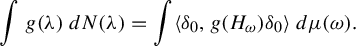(10) $$ \begin{align} \int g(\unicode{x3bb})\,dN(\unicode{x3bb}) = \int \langle \delta_0 , g(H_{\omega}) \delta_0 \rangle \, d\mu(\omega). \end{align} $$

The integrated density of states (IDS), N, is then given by

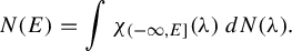(11) $$ \begin{align} N(E) = \int \chi_{(- \infty, E]} (\unicode{x3bb}) \, dN(\unicode{x3bb}). \end{align} $$

The terminology is explained by the fact that

(12) $$ \begin{align} N(E) = \lim_{n \to \infty} \frac{\# \{ \text{eigenvalues of } H_{\omega,[1,n]} \le E \}}{n} \quad \text{ for } \mu\text{-a.e.} \ \omega \in \Omega, \end{align} $$

where $H_{\omega ,[1,n]}$ denotes the restriction of $H_{\omega }$ to the interval $[1,n]$ with Dirichlet boundary conditions. It is a basic result that the IDS is always continuous [Reference Avron and SimonAS, Reference PasturPa], [Reference Damanik and FillmanDF1, Theorem 4.3.6]; see [Reference Delyon and SouillardDS2] for a very short proof that also works in higher dimensions. For specific models, explicit moduli of continuity can be established. For example, for the free Laplacian, we have

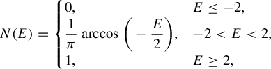$$ \begin{equation*}N(E) = \left\{\begin{array}{@{}l@{\quad}l} 0, & E \le -2, \\ \displaystyle\frac{1}{\pi} \mbox{ arccos } \bigg(\displaystyle - \frac{E}{2} \bigg), & -2 < E < 2, \\ 1, & E \ge 2, \end{array}\right.\end{equation*} $$

which is Hölder continuous. For the Anderson model (that is, for Schrödinger operators with (independent and identically distributed (iid) random potentials), it is known that the IDS must be Hölder continuous [Reference Le PageL], and under additional assumptions of regularity of the distribution that defines the potential, stronger results are available [Reference KirschKi, Reference Klein and SpeisKS, Reference Simon and TaylorST]. In particular, in the case of compactly supported distribution with polynomially decaying Fourier transform, one can show that the IDS must be $C^\infty $ , see [Reference Campanino and KleinCK]. For the Fibonacci Hamiltonian, the IDS must be Hölder continuous [Reference Damanik and GorodetskiDG1], while it is not always the case for operators with Sturmian potentials, see [Reference MungerMun] for details. Hölder continuity of the IDS in the case of quasiperiodic potentials was established in [Reference Goldstein and SchlagGS].

Many spectral properties of the operator in equation (9), including the integrated density of states, can be expressed in terms of the corresponding Schrödinger cocycle. To define it, for each $\omega \in \mathfrak {M}$ and $E\in \mathbb {R}$ , introduce the transfer matrix

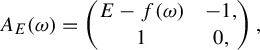$$ \begin{align*} A_E(\omega)=\begin{pmatrix} E-f(\omega) & -1, \\ 1 & 0, \\ \end{pmatrix}, \end{align*} $$

and consider the $SL(2, \mathbb {R})$ cocycle

$$ \begin{align*} (\sigma, A_E):\mathfrak{M}\times \mathbb{R}^2\to \mathfrak{M}\times\mathbb{R}^2, (\omega, \bar v)\mapsto (\sigma(\omega), A_E(\omega)\bar v), \end{align*} $$

usually called a Schrödinger cocycle corresponding to the family in equation (9). Each linear map $A_E(\omega )$ induces a projective map that we will denote by $g_{E, \omega }:\mathbb {RP}^1\to \mathbb {RP}^1$ . It is not hard to see that in the case of bounded function f, if $|E|\gg 1$ , then the cocycle in equation (1) is uniformly hyperbolic. In this case, one can choose the lifts $\tilde {g}_{E, \omega }$ in such a way that the rotation number $\rho (E)$ of the corresponding cocycle is equal to 0 for $E\gg 1$ and to $1/2$ for $E\ll -1$ . For a measurable function f, one can choose lifts in such a way that $\rho (E)\to 0$ as $E\to +\infty $ and $\rho (E)\to 1/2$ as $E\to -\infty $ . In either case, the integrated density of states $N(E)$ can be expressed via the rotation number [Reference Delyon and SouillardDS1]:

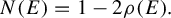$$ \begin{align*} N(E)=1-2\rho(E). \end{align*} $$

Together with Theorem 2.5, this immediately gives a purely dynamical proof of the following statement.

Theorem 3.1. (Theorem 5.2 from [Reference Craig and SimonCS2])

In the setting above, if the function ${f:\mathfrak {M}\to \mathbb {R}^1}$ is such that

$$ \begin{align*} \int_{\mathfrak{M}}\log(1+ |f(\omega)|)\,d\mu <\infty, \end{align*} $$

then the integrated density of states $N(E)$ is $\mathrm {log}$ -Hölder continuous, that is, for any compact $J\subset \mathbb {R}$ , for some $C>0$ , and any $E_1, E_2\in J$ with $|E_1-E_2|\le 1/2$ , one has

$$ \begin{align*} | N(E_1) - N(E_2) | \le C ( \log |E_1 - E_2|^{-1} )^{-1}. \end{align*} $$

A multidimensional version of this statement was provided in [Reference Craig and SimonCS1]. In both [Reference Craig and SimonCS1] and [Reference Craig and SimonCS2], the Thouless formula is used as the main tool. The Thouless formula relates the integrated density of states of an ergodic family of Schrödiger operators and the Lyapunov exponent of the corresponding Schrödinger cocycle; in the nonlinear setting of Theorem 2.5, one of the parts of this formula, the Lyapunov exponent, is just not defined. Notice that the original results [Reference Craig and SimonCS1, Reference Craig and SimonCS2] deal with bounded potentials only, but in [Reference Craig and SimonCS1], the authors make a remark that their method can be adapted to the case when the function $\log (1+|f|)$ belongs to the space $L^1$ .

An analog of Theorem 3.1 for CMV matrices was provided in [Reference Fillman and OngFO]. Also, in many models, the regularity of Lyapunov exponent of the corresponding linear cocycle is related to the regularity of the integrated density of states, and the former was heavily studied, e.g. see [Reference Bourgain and JitomirskayaBJ, Reference Duarte and KleinDK, Reference Duarte, Klein and PolettiDKP], just to give a few examples.

The question whether Theorem 3.1 is optimal was heavily discussed in spectral theory of ergodic Schrödinger operators. It turned out that the modulus of continuity of the integrated density of states in general cannot be improved. It was shown that even for the Anderson model, the integrated density of states does not have to be Hölder continuous with a given power [Reference HalperinHal]. Also, [Reference CraigCr, Theorem 5] essentially claims that for any continuous increasing function $N(E)$ on $[0,1]$ with $N(0)=0, N(1)=1$ that is $\alpha $ -log-Hölder continuous with any $\alpha>1$ , that is, just slightly more regular than allowed by Theorem 3.1, there exists a family of almost periodic Schrödinger operators with an integrated density of states given by the function $N(E)$ . Finally, in [Reference Krüger and GanKG], the limit periodic potentials were used to show that Theorem 3.1 is sharp, and an estimate in Theorem 3.1 cannot be replaced by any better modulus of continuity. Later examples in other special classes of ergodic Schrödinger operators were constructed as well. So, in [Reference Duarte, Klein and SantosDKS], an example in the class of random Schrödinger cocycles was constructed, and in [Reference Avila, Last, Shamis and ZhouALSZ]—in the class of quasiperiodic operators. In particular, these results imply that the modulus of continuity in Theorem 2.5 is also optimal.