


1 Introduction
The Birch–Swinnerton-Dyer conjecture relates the Hasse–Weil L-function $ L(E, s) $
of an elliptic curve
$ L(E, s) $
of an elliptic curve $ E $
over
$ E $
over $ \mathbb {Q} $
to certain algebraic invariants that encode important global arithmetic information of
$ \mathbb {Q} $
to certain algebraic invariants that encode important global arithmetic information of $ E $
[Reference Wiles34]. Over a finite extension
$ E $
[Reference Wiles34]. Over a finite extension $ K $
of
$ K $
of $ \mathbb {Q} $
, Artin’s formalism for L-functions says that the Hasse–Weil L-function
$ \mathbb {Q} $
, Artin’s formalism for L-functions says that the Hasse–Weil L-function $ L(E / K, s) $
of
$ L(E / K, s) $
of $ E $
base changed to
$ E $
base changed to $ K $
decomposes into a finite product of certain twisted L-functions
$ K $
decomposes into a finite product of certain twisted L-functions $ L(E, \chi , s) $
, ranging over all Artin representations
$ L(E, \chi , s) $
, ranging over all Artin representations $ \chi $
that factor through
$ \chi $
that factor through $ K $
, so that the behavior of
$ K $
, so that the behavior of $ L(E / K, s) $
is completely governed by
$ L(E / K, s) $
is completely governed by $ L(E, \chi , s) $
. The algebraic and analytic properties of these twisted L-functions are studied extensively in the literature, and they are the subject of many important open problems in the arithmetic of elliptic curves, most notably equivariant refinements of the Birch–Swinnerton-Dyer conjecture [Reference Burns and Castillo5].
$ L(E, \chi , s) $
. The algebraic and analytic properties of these twisted L-functions are studied extensively in the literature, and they are the subject of many important open problems in the arithmetic of elliptic curves, most notably equivariant refinements of the Birch–Swinnerton-Dyer conjecture [Reference Burns and Castillo5].
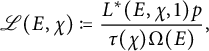
The special value $ L^*(E, \chi , 1) $
of
$ L^*(E, \chi , 1) $
of $ L(E, \chi , s) $
at
$ L(E, \chi , s) $
at $ s = 1 $
can be normalized by certain factors to get a modified twisted L-value
$ s = 1 $
can be normalized by certain factors to get a modified twisted L-value $ \mathscr {L}(E, \chi ) $
that is conjectured to have nice algebraic properties. When
$ \mathscr {L}(E, \chi ) $
that is conjectured to have nice algebraic properties. When $ \chi = 1 $
is the trivial representation,
$ \chi = 1 $
is the trivial representation, $ \mathscr {L}(E, \chi ) $
is simply given by the special value of
$ \mathscr {L}(E, \chi ) $
is simply given by the special value of $ L(E, s) $
at
$ L(E, s) $
at $ s = 1 $
divided by the real period
$ s = 1 $
divided by the real period $ \Omega (E) $
. When
$ \Omega (E) $
. When $ \chi $
is a nontrivial even Dirichlet character of prime conductor
$ \chi $
is a nontrivial even Dirichlet character of prime conductor $ p $
, this is given by
$ p $
, this is given by
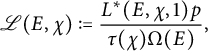
where $ \tau (\chi ) $
is the Gauss sum of
$ \tau (\chi ) $
is the Gauss sum of $ \chi $
.
$ \chi $
.
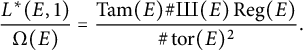
Classically, Birch and Swinnerton-Dyer conjectured that $ \mathscr {L}(E, 1) = \operatorname {BSD}(E) $
, where
$ \mathscr {L}(E, 1) = \operatorname {BSD}(E) $
, where $ \operatorname {BSD}(E) $
is the Birch–Swinnerton-Dyer quotient
$ \operatorname {BSD}(E) $
is the Birch–Swinnerton-Dyer quotient
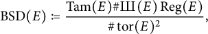
where $ \operatorname {Tam}(E) $
,
$ \operatorname {Tam}(E) $
, ![]() , and
, and $ \operatorname {Reg}(E) $
is the Tamagawa number, the Tate–Shafarevich group, and the elliptic regulator respectively. In contrast, there seems to be a barrier in formulating an analogous conjecture for
$ \operatorname {Reg}(E) $
is the Tamagawa number, the Tate–Shafarevich group, and the elliptic regulator respectively. In contrast, there seems to be a barrier in formulating an analogous conjecture for $ \mathscr {L}(E, \chi ) $
when
$ \mathscr {L}(E, \chi ) $
when $ \chi $
is nontrivial, with concrete examples of arithmetically identical elliptic curves with modified twisted L-values that differ by a unit [Reference Dokchitser, Evans and Wiersema12, Section 4]. Having such a formula would present nontrivial consequences for the arithmetic of
$ \chi $
is nontrivial, with concrete examples of arithmetically identical elliptic curves with modified twisted L-values that differ by a unit [Reference Dokchitser, Evans and Wiersema12, Section 4]. Having such a formula would present nontrivial consequences for the arithmetic of $ E / K $
, such as predictions for the non triviality of Tate–Shafarevich groups and the existence of points of infinite order, which are intractable with classical techniques for Selmer groups [Reference Dokchitser, Evans and Wiersema12, Section 3].
$ E / K $
, such as predictions for the non triviality of Tate–Shafarevich groups and the existence of points of infinite order, which are intractable with classical techniques for Selmer groups [Reference Dokchitser, Evans and Wiersema12, Section 3].
Prominent existing techniques to study the $ \ell $
-primary parts of Selmer groups, such as via the Iwasawa main conjectures, only gives a description of the ideal
$ \ell $
-primary parts of Selmer groups, such as via the Iwasawa main conjectures, only gives a description of the ideal $ I $
generated by
$ I $
generated by $ \mathscr {L}(E, \chi ) $
, rather than its actual value. In a recent paper to understand a refinement of the classical Birch–Swinnerton-Dyer conjecture, Burns–Castillo determined
$ \mathscr {L}(E, \chi ) $
, rather than its actual value. In a recent paper to understand a refinement of the classical Birch–Swinnerton-Dyer conjecture, Burns–Castillo determined $ I $
in terms of arithmetic invariants of
$ I $
in terms of arithmetic invariants of $ E $
in certain relative K-groups [Reference Burns and Castillo5, Proposition 7.3]. More concretely, Dokchitser–Evans–Wiersema expressed the norm of
$ E $
in certain relative K-groups [Reference Burns and Castillo5, Proposition 7.3]. More concretely, Dokchitser–Evans–Wiersema expressed the norm of $ I $
in terms of
$ I $
in terms of $ \operatorname {BSD}(E) $
and its base-changed quotient
$ \operatorname {BSD}(E) $
and its base-changed quotient $ \operatorname {BSD}(E / K) $
, where
$ \operatorname {BSD}(E / K) $
, where $ K $
is the number field cut out by
$ K $
is the number field cut out by $ \chi $
[Reference Dokchitser, Evans and Wiersema12, Theorem 38], but the actual value of
$ \chi $
[Reference Dokchitser, Evans and Wiersema12, Theorem 38], but the actual value of $ \mathscr {L}(E, \chi ) $
remains elusive.
$ \mathscr {L}(E, \chi ) $
remains elusive.
This article completely determines the actual value of $ \mathscr {L}(E, \chi ) $
for cubic Dirichlet characters of prime conductor, under fairly generic assumptions on the Manin constants
$ \mathscr {L}(E, \chi ) $
for cubic Dirichlet characters of prime conductor, under fairly generic assumptions on the Manin constants $ c_0(E) $
and
$ c_0(E) $
and $ c_1(E) $
, culminating in the following result proven in Section 5.
$ c_1(E) $
, culminating in the following result proven in Section 5.
Theorem 1.1 (Corollary 5.2)
Let $ E $
be an elliptic curve over
$ E $
be an elliptic curve over $ \mathbb {Q} $
of conductor
$ \mathbb {Q} $
of conductor $ N $
such that
$ N $
such that $ L(E, 1) \ne 0 $
. Let
$ L(E, 1) \ne 0 $
. Let $ \chi $
be a cubic Dirichlet character of odd prime conductor
$ \chi $
be a cubic Dirichlet character of odd prime conductor $ p \nmid N $
such that
$ p \nmid N $
such that $ 3 \nmid c_0(E)\operatorname {BSD}(E)\#E(\mathbb {F}_p) $
. Assume further that
$ 3 \nmid c_0(E)\operatorname {BSD}(E)\#E(\mathbb {F}_p) $
. Assume further that $ c_1(E) = 1 $
and that the Birch–Swinnerton-Dyer conjecture holds over number fields. Then
$ c_1(E) = 1 $
and that the Birch–Swinnerton-Dyer conjecture holds over number fields. Then
 $$ \begin{align*}\mathscr{L}(E, \chi) = u\overline{\chi(N)}B,\end{align*} $$
where the positive rational number $ B \in \mathbb {Q}^\times $
is the positive square root of the positive rational square
$ B \in \mathbb {Q}^\times $
is the positive square root of the positive rational square $ \operatorname {BSD}(E / K) / \operatorname {BSD}(E) \in (\mathbb {Q}^\times )^2 $
, and the sign
$ \operatorname {BSD}(E / K) / \operatorname {BSD}(E) \in (\mathbb {Q}^\times )^2 $
, and the sign $ u = \pm 1 $
is such that
$ u = \pm 1 $
is such that
 $$ \begin{align*}u \equiv -\#E(\mathbb{F}_p)\operatorname{BSD}(E)B^{-1} \quad\mod 3.\end{align*} $$
On the analytic side of things, in a paper on an analog of the Brauer–Siegel theorem for elliptic curves over cyclic extensions, Kisilevsky–Nam observed some patterns in the asymptotic distribution of $ \mathscr {L}(E, \chi ) $
[Reference Kisilevsky and Nam18, Section 7]. They considered six elliptic curves
$ \mathscr {L}(E, \chi ) $
[Reference Kisilevsky and Nam18, Section 7]. They considered six elliptic curves $ E $
and five positive integers
$ E $
and five positive integers $ q $
, and numerically computed the norms of
$ q $
, and numerically computed the norms of $ \mathscr {L}(E, \chi ) $
for primitive Dirichlet characters
$ \mathscr {L}(E, \chi ) $
for primitive Dirichlet characters $ \chi $
of conductor
$ \chi $
of conductor $ p $
and order
$ p $
and order $ q $
, ranging over the thirty pairs of
$ q $
, ranging over the thirty pairs of $ (E, q) $
and millions of positive integers
$ (E, q) $
and millions of positive integers $ p $
. For each pair of
$ p $
. For each pair of $ (E, q) $
, they added a normalization factor to
$ (E, q) $
, they added a normalization factor to $ \mathscr {L}(E, \chi ) $
to obtain a real L-value
$ \mathscr {L}(E, \chi ) $
to obtain a real L-value $ \mathscr {L}^+(E, \chi ) $
, and empirically determined the greatest common divisor
$ \mathscr {L}^+(E, \chi ) $
, and empirically determined the greatest common divisor $ \gcd _{E, q} $
of the norms of
$ \gcd _{E, q} $
of the norms of $ \mathscr {L}^+(E, \chi ) $
by varying over all
$ \mathscr {L}^+(E, \chi ) $
by varying over all $ p $
. Upon dividing these norms by
$ p $
. Upon dividing these norms by $ \gcd _{E, q} $
, they observed that these integers have unexpected biases when reduced modulo
$ \gcd _{E, q} $
, they observed that these integers have unexpected biases when reduced modulo $ q $
.
$ q $
.
This article completely predicts these biases for cubic Dirichlet characters of prime conductor, again under fairly generic assumptions, for three of the six elliptic curves they considered. The following result is proven under slightly relaxed assumptions in Section 7, where the normalization for $ \mathscr {L}^+(E, \chi ) $
is also defined.
$ \mathscr {L}^+(E, \chi ) $
is also defined.
Theorem 1.2 (Proposition 7.7)
Let $ E $
be an elliptic curve over
$ E $
be an elliptic curve over $ \mathbb {Q} $
of conductor
$ \mathbb {Q} $
of conductor $ N $
and minimal discriminant
$ N $
and minimal discriminant $ \Delta = \pm N^n $
for some
$ \Delta = \pm N^n $
for some $ n \in \mathbb {N} $
, such that
$ n \in \mathbb {N} $
, such that $ E $
has no rational
$ E $
has no rational $ 3 $
-isogeny and that
$ 3 $
-isogeny and that $ 3 \nmid nc_0(E)\gcd _{E, 3} $
. Let
$ 3 \nmid nc_0(E)\gcd _{E, 3} $
. Let $ \chi $
be a cubic Dirichlet character of odd prime conductor
$ \chi $
be a cubic Dirichlet character of odd prime conductor $ p \nmid N $
. Then
$ p \nmid N $
. Then
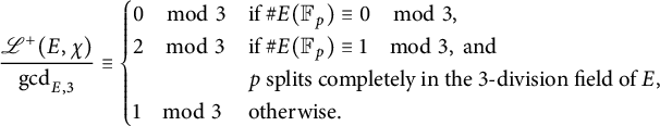 $$ \begin{align*}\dfrac{\mathscr{L}^+(E, \chi)}{\gcd_{E, 3}} \equiv \begin{cases} 0\quad \mod 3 & \text{if} \ \#E(\mathbb{F}_p) \equiv 0 \quad\mod 3, \\ 2\quad \mod 3 & \text{if} \ \#E(\mathbb{F}_p) \equiv 1 \quad\mod 3, \ \text{and} \\ & p \ \text{splits completely in the } 3 \text{-division field of} \ E, \\ 1\quad \mod 3 & \text{otherwise}. \end{cases} \end{align*} $$
To put things in a more structured perspective, these biases can be quantified asymptotically by considering the natural densities of $ \mathscr {L}(E, \chi ) $
when reduced modulo
$ \mathscr {L}(E, \chi ) $
when reduced modulo $ q $
. More precisely, let
$ q $
. More precisely, let $ X_{E, q}^{< n} $
be the set of Dirichlet characters of odd order
$ X_{E, q}^{< n} $
be the set of Dirichlet characters of odd order $ q> 1 $
and odd prime conductor
$ q> 1 $
and odd prime conductor $ p < n $
such that
$ p < n $
such that $ p $
does not divide the conductor of
$ p $
does not divide the conductor of $ E $
. Now define the residual densities
$ E $
. Now define the residual densities $ \delta _{E, q} $
of
$ \delta _{E, q} $
of $ \mathscr {L}(E, \chi ) $
to be the natural densities of
$ \mathscr {L}(E, \chi ) $
to be the natural densities of $ \mathscr {L}(E, \chi ) $
modulo
$ \mathscr {L}(E, \chi ) $
modulo $ (1 - \zeta _q) $
. In other words, this is the value
$ (1 - \zeta _q) $
. In other words, this is the value
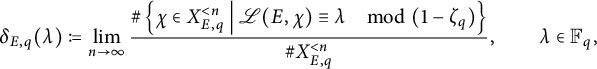
if such a limit exists. It turns out that such a limit always exists, and its value for any $ \lambda \in \mathbb {F}_q $
only depends on
$ \lambda \in \mathbb {F}_q $
only depends on $ \operatorname {BSD}(E) $
, the torsion subgroup
$ \operatorname {BSD}(E) $
, the torsion subgroup $ \operatorname {tor}(E) $
, and the mod-
$ \operatorname {tor}(E) $
, and the mod- $ q^2 $
Galois image
$ q^2 $
Galois image $ \operatorname {im}(\overline {\rho _{E, q^2}}) $
. The following result classifies the possible residual densities for cubic Dirichlet characters, namely the ordered triples
$ \operatorname {im}(\overline {\rho _{E, q^2}}) $
. The following result classifies the possible residual densities for cubic Dirichlet characters, namely the ordered triples
Theorem 1.3 (Theorem 6.4)
Let $ E $
be an elliptic curve over
$ E $
be an elliptic curve over $ \mathbb {Q} $
such that
$ \mathbb {Q} $
such that $ L(E, 1) \ne 0 $
and that
$ L(E, 1) \ne 0 $
and that $ 3 \nmid c_0(E) $
. Assume further that the Birch–Swinnerton-Dyer conjecture holds. Then
$ 3 \nmid c_0(E) $
. Assume further that the Birch–Swinnerton-Dyer conjecture holds. Then $ \delta _{E, 3} $
only depends on
$ \delta _{E, 3} $
only depends on $ \operatorname {BSD}(E) $
and on
$ \operatorname {BSD}(E) $
and on $ \operatorname {im}(\overline {\rho _{E, 9}}) $
, and can only be one of
$ \operatorname {im}(\overline {\rho _{E, 9}}) $
, and can only be one of
 $$ \begin{align*}(1, 0, 0), \ \left(\tfrac{3}{8}, \tfrac{3}{8}, \tfrac{1}{4}\right), \ \left(\tfrac{3}{8}, \tfrac{1}{4}, \tfrac{3}{8}\right), \ \left(\tfrac{1}{2}, \tfrac{1}{2}, 0\right), \ \left(\tfrac{1}{2}, 0, \tfrac{1}{2}\right), \ \left(\tfrac{1}{8}, \tfrac{3}{4}, \tfrac{1}{8}\right),\end{align*} $$
 $$ \begin{align*}\left(\tfrac{1}{8}, \tfrac{1}{8}, \tfrac{3}{4}\right), \ \left(\tfrac{1}{4}, \tfrac{1}{2}, \tfrac{1}{4}\right), \ \left(\tfrac{1}{4}, \tfrac{1}{4}, \tfrac{1}{2}\right), \ \left(\tfrac{5}{9}, \tfrac{2}{9}, \tfrac{2}{9}\right), \ \left(\tfrac{1}{3}, \tfrac{2}{3}, 0\right), \ \left(\tfrac{1}{3}, 0, \tfrac{2}{3}\right).\end{align*} $$
In particular, $ \delta _{E, 3} $
can be determined as follows.
$ \delta _{E, 3} $
can be determined as follows.
-
• If $ \operatorname {ord}_3(\operatorname {BSD}(E)) = 0 $
and
$ 3 \nmid \#\operatorname {tor}(E) $
, then
$ \delta _{E, 3} $
is given by the table in Section A.1.
$ \operatorname {ord}_3(\operatorname {BSD}(E)) = 0 $
and
$ 3 \nmid \#\operatorname {tor}(E) $
, then
$ \delta _{E, 3} $
is given by the table in Section A.1. -
• If
$ \operatorname {ord}_3(\operatorname {BSD}(E)) = -1 $
, then
$ \delta _{E, 3} $
is given by the table in Section A.2. -
• Otherwise,
$ \delta _{E, 3} = (1, 0, 0) $
.


Note that the aforementioned normalization factors are not present here, so that the resulting residual densities will be different from that of Kisilevsky–Nam. Section 6 proves this result and outlines the general procedure for higher order characters.
This classification builds upon the independent result that $ \operatorname {ord}_3(\operatorname {BSD}(E)) \ge -1 $
. In a seminal paper quantifying the cancellations between
$ \operatorname {ord}_3(\operatorname {BSD}(E)) \ge -1 $
. In a seminal paper quantifying the cancellations between $ \operatorname {tor}(E) $
and
$ \operatorname {tor}(E) $
and $ \operatorname {Tam}(E) $
, Lorenzini proved that if a prime
$ \operatorname {Tam}(E) $
, Lorenzini proved that if a prime $ \ell> 3 $
is such that
$ \ell> 3 $
is such that $ \ell \mid \#\operatorname {tor}(E) $
, then
$ \ell \mid \#\operatorname {tor}(E) $
, then $ \ell \mid \operatorname {Tam}(E) $
with finitely many explicit exceptions [Reference Lorenzini20, Proposition 1.1]. In particular, when
$ \ell \mid \operatorname {Tam}(E) $
with finitely many explicit exceptions [Reference Lorenzini20, Proposition 1.1]. In particular, when $ E $
has analytic rank zero, the denominator
$ E $
has analytic rank zero, the denominator $ \#\operatorname {tor}(E)^2 $
of the rational number
$ \#\operatorname {tor}(E)^2 $
of the rational number $ \operatorname {BSD}(E) $
necessarily shares a factor with
$ \operatorname {BSD}(E) $
necessarily shares a factor with $ \operatorname {Tam}(E) $
in its numerator, so that
$ \operatorname {Tam}(E) $
in its numerator, so that $ \operatorname {ord}_\ell (\operatorname {BSD}(E)) \ge -1 $
for any prime
$ \operatorname {ord}_\ell (\operatorname {BSD}(E)) \ge -1 $
for any prime $ \ell> 3 $
. On the other hand, he noted that there are explicit families with
$ \ell> 3 $
. On the other hand, he noted that there are explicit families with $ \#\operatorname {tor}(E) = 3 $
without any cancellation [Reference Lorenzini20, Lemma 2.26], another family of which was given by Barrios–Roy [Reference Barrios and Roy1, Corollary 5.1]. Subsequently, Melistas showed that these cancellations may instead occur between
$ \#\operatorname {tor}(E) = 3 $
without any cancellation [Reference Lorenzini20, Lemma 2.26], another family of which was given by Barrios–Roy [Reference Barrios and Roy1, Corollary 5.1]. Subsequently, Melistas showed that these cancellations may instead occur between $ \operatorname {tor}(E) $
and
$ \operatorname {tor}(E) $
and ![]() in the numerator of
in the numerator of $ \operatorname {BSD}(E) $
, and hence
$ \operatorname {BSD}(E) $
, and hence $ \operatorname {ord}_3(\operatorname {BSD}(E)) \ge -1 $
, except possibly for certain reduction types [Reference Melistas23, Theorem 1.4]. He then observed that there are again explicit exceptions, and in all these exceptions
$ \operatorname {ord}_3(\operatorname {BSD}(E)) \ge -1 $
, except possibly for certain reduction types [Reference Melistas23, Theorem 1.4]. He then observed that there are again explicit exceptions, and in all these exceptions $ c_0(E) = 3 $
[Reference Melistas23, Example 3.8], but did not explain this coincidence. The following result gives a lower bound for the odd part of the denominator of
$ c_0(E) = 3 $
[Reference Melistas23, Example 3.8], but did not explain this coincidence. The following result gives a lower bound for the odd part of the denominator of $ \operatorname {BSD}(E) $
.
$ \operatorname {BSD}(E) $
.
Theorem 1.4 (Theorem 4.4)
Let $ E $
be an elliptic curve over
$ E $
be an elliptic curve over $ \mathbb {Q} $
such that
$ \mathbb {Q} $
such that $ {L(E, 1) \ne 0} $
. Let
$ {L(E, 1) \ne 0} $
. Let $ \ell $
be an odd prime such that
$ \ell $
be an odd prime such that $ \ell \nmid c_0(E) $
. Assume further that the Birch–Swinnerton-Dyer conjecture holds. If
$ \ell \nmid c_0(E) $
. Assume further that the Birch–Swinnerton-Dyer conjecture holds. If $ \ell \mid \#\operatorname {tor}(E) $
, then
$ \ell \mid \#\operatorname {tor}(E) $
, then ![]() . In particular,
. In particular, $ \operatorname {ord}_\ell (\operatorname {BSD}(E)) \ge -1 $
.
$ \operatorname {ord}_\ell (\operatorname {BSD}(E)) \ge -1 $
.
Section 4 states this result in terms of $ \mathscr {L}(E, 1) $
and proves it in slightly larger generality. Note that this is related to the Gross–Zagier conjecture for
$ \mathscr {L}(E, 1) $
and proves it in slightly larger generality. Note that this is related to the Gross–Zagier conjecture for $ \#\operatorname {tor}(E) = 3 $
proven by Byeon–Kim–Yhee [Reference Byeon, Kim and Yhee9, Theorem 1.2], but their divisibility result holds over imaginary quadratic fields with a Heegner point of infinite order. In particular, the local computations here are a subset of their local Tamagawa number computations, but the global divisibility argument here uses the integrality of
$ \#\operatorname {tor}(E) = 3 $
proven by Byeon–Kim–Yhee [Reference Byeon, Kim and Yhee9, Theorem 1.2], but their divisibility result holds over imaginary quadratic fields with a Heegner point of infinite order. In particular, the local computations here are a subset of their local Tamagawa number computations, but the global divisibility argument here uses the integrality of $ \mathscr {L}(E, 1) $
instead.
$ \mathscr {L}(E, 1) $
instead.
The methods in this article rely on the key fact that $ \mathscr {L}(E, \chi ) \in \mathbb {Z}[\zeta _q] $
for nontrivial primitive Dirichlet characters
$ \mathscr {L}(E, \chi ) \in \mathbb {Z}[\zeta _q] $
for nontrivial primitive Dirichlet characters $ \chi $
of order
$ \chi $
of order $ q $
, which was proven by Wiersema–Wuthrich under some mild hypotheses by expressing
$ q $
, which was proven by Wiersema–Wuthrich under some mild hypotheses by expressing $ \mathscr {L}(E, \chi ) $
in terms of Manin’s modular symbols [Reference Wiersema and Wuthrich33, Theorem 2]. Parts of their argument can be adapted to obtain an explicit congruence between
$ \mathscr {L}(E, \chi ) $
in terms of Manin’s modular symbols [Reference Wiersema and Wuthrich33, Theorem 2]. Parts of their argument can be adapted to obtain an explicit congruence between $ \mathscr {L}(E, \chi ) $
and
$ \mathscr {L}(E, \chi ) $
and $ \mathscr {L}(E, 1) $
modulo the prime
$ \mathscr {L}(E, 1) $
modulo the prime $ (1 - \zeta _q) $
in
$ (1 - \zeta _q) $
in $ \mathbb {Z}[\zeta _q] $
above
$ \mathbb {Z}[\zeta _q] $
above $ q $
. After establishing notational conventions in Section 2, some background on Manin’s modular symbols will be provided in Section 3 to obtain this congruence. The remaining sections will be devoted to proving the four aforementioned results, with an appendix consisting of a list of mod-
$ q $
. After establishing notational conventions in Section 2, some background on Manin’s modular symbols will be provided in Section 3 to obtain this congruence. The remaining sections will be devoted to proving the four aforementioned results, with an appendix consisting of a list of mod- $ 3 $
and
$ 3 $
and $ 3 $
-adic Galois images.
$ 3 $
-adic Galois images.
2 Background and conventions
This section establishes some relevant background on Galois representations and L-functions of elliptic curves and Dirichlet characters, as well as some notational conventions that might be deemed less standard in the literature.
For a primitive $ n $
th root of unity
$ n $
th root of unity $ \zeta _n $
, the ring of integers of the cyclotomic field
$ \zeta _n $
, the ring of integers of the cyclotomic field $ \mathbb {Q}(\zeta _n) $
will be denoted
$ \mathbb {Q}(\zeta _n) $
will be denoted $ \mathbb {Z}[\zeta _n] $
, and denote its norm map by
$ \mathbb {Z}[\zeta _n] $
, and denote its norm map by $ \operatorname {Nm}_n : \mathbb {Q}(\zeta _n) \to \mathbb {Q} $
. The ring of integers of its maximal totally real subfield
$ \operatorname {Nm}_n : \mathbb {Q}(\zeta _n) \to \mathbb {Q} $
. The ring of integers of its maximal totally real subfield $ \mathbb {Q}(\zeta _n)^+ $
will be denoted
$ \mathbb {Q}(\zeta _n)^+ $
will be denoted $ \mathbb {Z}[\zeta _n]^+ $
, and denote its norm map by
$ \mathbb {Z}[\zeta _n]^+ $
, and denote its norm map by $ \operatorname {Nm}_n^+ : \mathbb {Q}(\zeta _n)^+ \to \mathbb {Q} $
. The isomorphism in class field theory from the unit group
$ \operatorname {Nm}_n^+ : \mathbb {Q}(\zeta _n)^+ \to \mathbb {Q} $
. The isomorphism in class field theory from the unit group $ (\mathbb {Z} / n)^\times $
of
$ (\mathbb {Z} / n)^\times $
of $ \mathbb {Z} $
modulo
$ \mathbb {Z} $
modulo $ n $
to the cyclotomic Galois group
$ n $
to the cyclotomic Galois group $ \operatorname {Gal}(\mathbb {Q}(\zeta _n) / \mathbb {Q}) $
will be given by
$ \operatorname {Gal}(\mathbb {Q}(\zeta _n) / \mathbb {Q}) $
will be given by $ a \mapsto (\zeta _n \mapsto \zeta _n^a) $
, which identifies Dirichlet characters of modulus
$ a \mapsto (\zeta _n \mapsto \zeta _n^a) $
, which identifies Dirichlet characters of modulus $ n $
with Artin representations that factor through
$ n $
with Artin representations that factor through $ \mathbb {Q}(\zeta _n) $
.
$ \mathbb {Q}(\zeta _n) $
.
Denote the two-dimensional special, general, and projective linear group functors by $ \operatorname {SL}_2 $
,
$ \operatorname {SL}_2 $
, $ \operatorname {GL}_2 $
, and
$ \operatorname {GL}_2 $
, and $ \operatorname {PGL}_2 $
. For a matrix
$ \operatorname {PGL}_2 $
. For a matrix $ M $
in such a matrix group, its trace will be denoted
$ M $
in such a matrix group, its trace will be denoted $ \operatorname {tr}(M) $
and its determinant will be denoted
$ \operatorname {tr}(M) $
and its determinant will be denoted $ \det (M) $
. For a prime
$ \det (M) $
. For a prime $ \ell $
, the conjugacy classes of
$ \ell $
, the conjugacy classes of $ \operatorname {SL}_2(\mathbb {Z} / \ell ) $
can be grouped by their traces as follows [Reference Bonnafé3, Table 1.1 and Exercise 1.4].
$ \operatorname {SL}_2(\mathbb {Z} / \ell ) $
can be grouped by their traces as follows [Reference Bonnafé3, Table 1.1 and Exercise 1.4].
-
• There are three conjugacy classes of trace
$ 2 $
represented by
$ (\begin {smallmatrix} 1 & z \\ 0 & 1 \end {smallmatrix}) $
for
$ z \in \mathbb {F}_\ell $
, one for each of the three Legendre symbols
$ \left (\tfrac {z}{\ell }\right ) \in \{0, \pm 1\} $
, each of which has cardinality equal to
$ ((\ell ^2 - 1) / 2)^{\left |\left (\frac {z}{\ell }\right )\right |} $
and has elements of order equal to
$ \ell ^{\left |\left (\frac {z}{\ell }\right )\right |} $
. -
• There are three conjugacy classes of trace
$ \ell - 2 $
represented by
$ (\begin {smallmatrix} -1 & z \\ 0 & -1 \end {smallmatrix}) $
for
$ z \in \mathbb {F}_\ell $
, one for each of the three Legendre symbols
$ \left (\tfrac {z}{\ell }\right ) \in \{0, \pm 1\} $
, each of which has cardinality equal to
$ ((\ell ^2 - 1) / 2)^{\left |\left (\frac {z}{\ell }\right )\right |} $
and has elements of order equal to
$ 2\ell ^{\left |\left (\frac {z}{\ell }\right )\right |} $
. -
• There are
$ (\ell - 3) / 2 $
conjugacy classes of trace
$ x + x^{-1} $
represented by
$ (\begin {smallmatrix} x & 0 \\ 0 & x^{-1} \end {smallmatrix}) $
for
$ x \in \mathbb {F}_\ell ^\times \setminus \{\pm 1\} $
, one for each unordered pair
$ \{x^{\pm 1}\} $
, each of which has cardinality equal to
$ \ell (\ell + 1) $
and has elements of order equal to the order of
$ x $
. -
• There are
$ (\ell - 1) / 2 $
conjugacy classes of trace
$ \xi + \xi ^\ell $
represented by where
$$ \begin{align*}\begin{pmatrix} \tfrac{1}{2}(\xi + \xi^\ell) & \tfrac{\zeta}{2}(\xi - \xi^\ell) \\ \tfrac{1}{2\zeta}(\xi - \xi^\ell) & \tfrac{1}{2}(\xi + \xi^\ell) \end{pmatrix}, \qquad \xi \in (\mathbb{F}_{\ell^2}^\times / \mathbb{F}_\ell^\times) \setminus \{\pm1\},\end{align*} $$
$ \zeta $
is a fixed element of
$ \mathbb {F}_{\ell ^2}^\times $
satisfying
$ \zeta + \zeta ^\ell = 0 $
, one for each pair
$ \{\xi ^{\pm 1}\} $
, each of which has cardinality
$ \ell (\ell - 1) $
and elements of order equal to the order of
$ \xi $
.


This will be useful for Theorem 4.4 and Proposition 6.1.
Throughout, an elliptic curve will always refer to an elliptic curve $ E $
over
$ E $
over $ \mathbb {Q} $
of conductor
$ \mathbb {Q} $
of conductor $ N $
, and any explicit example of an elliptic curve will be given by its Cremona label [Reference Cremona11, Table 1]. For a prime
$ N $
, and any explicit example of an elliptic curve will be given by its Cremona label [Reference Cremona11, Table 1]. For a prime $ \ell $
, the
$ \ell $
, the $ \ell $
-adic Galois representation associated with the
$ \ell $
-adic Galois representation associated with the $ \ell $
-adic Tate module of
$ \ell $
-adic Tate module of $ E $
is denoted
$ E $
is denoted $ \rho _{E, \ell } $
, and its
$ \rho _{E, \ell } $
, and its $ \ell $
-adic Galois image
$ \ell $
-adic Galois image $ \operatorname {im}(\rho _{E, \ell }) $
will be given by its Rouse–Sutherland–Zureick-Brown label as a subgroup of
$ \operatorname {im}(\rho _{E, \ell }) $
will be given by its Rouse–Sutherland–Zureick-Brown label as a subgroup of $ \operatorname {GL}_2(\mathbb {Z}_\ell ) $
up to conjugacy [Reference Rouse, Sutherland and Zureick-Brown25, Section 2.4]. For any
$ \operatorname {GL}_2(\mathbb {Z}_\ell ) $
up to conjugacy [Reference Rouse, Sutherland and Zureick-Brown25, Section 2.4]. For any $ n \in \mathbb {N} $
, the projection of
$ n \in \mathbb {N} $
, the projection of $ \rho _{E, \ell } $
onto
$ \rho _{E, \ell } $
onto $ \operatorname {GL}_2(\mathbb {Z} / \ell ^n) $
is denoted
$ \operatorname {GL}_2(\mathbb {Z} / \ell ^n) $
is denoted $ \overline {\rho _{E, \ell ^n}} $
, and its mod-
$ \overline {\rho _{E, \ell ^n}} $
, and its mod- $ \ell ^n $
Galois image
$ \ell ^n $
Galois image $ \operatorname {im}(\overline {\rho _{E, \ell ^n}}) $
will be given by its Sutherland label as a subgroup of
$ \operatorname {im}(\overline {\rho _{E, \ell ^n}}) $
will be given by its Sutherland label as a subgroup of $ \operatorname {GL}_2(\mathbb {Z} / \ell ^n) $
up to conjugacy [Reference Sutherland31, Section 6.4]. Note that if
$ \operatorname {GL}_2(\mathbb {Z} / \ell ^n) $
up to conjugacy [Reference Sutherland31, Section 6.4]. Note that if $ \operatorname {Fr}_v $
is an arithmetic Frobenius at a prime
$ \operatorname {Fr}_v $
is an arithmetic Frobenius at a prime $ v \ne \ell $
, then its trace is given by
$ v \ne \ell $
, then its trace is given by
Let $ \omega _E $
denote a global invariant differential on a minimal Weierstrass equation of
$ \omega _E $
denote a global invariant differential on a minimal Weierstrass equation of $ E $
. Let
$ E $
. Let $ X_0(N) $
denote the modular curve associated with the Hecke congruence subgroup
$ X_0(N) $
denote the modular curve associated with the Hecke congruence subgroup $ \Gamma _0(N) $
of
$ \Gamma _0(N) $
of $ \operatorname {SL}_2(\mathbb {Z}) $
, and let
$ \operatorname {SL}_2(\mathbb {Z}) $
, and let $ S_2(N) $
denote the space of weight two cusp forms of level
$ S_2(N) $
denote the space of weight two cusp forms of level $ \Gamma _0(N) $
. By the modularity theorem, there is a surjective morphism
$ \Gamma _0(N) $
. By the modularity theorem, there is a surjective morphism $ \phi _E : X_0(N) \twoheadrightarrow E $
of minimal degree and an eigenform
$ \phi _E : X_0(N) \twoheadrightarrow E $
of minimal degree and an eigenform $ f_E \in S_2(N) $
with Fourier coefficients
$ f_E \in S_2(N) $
with Fourier coefficients $ a_v(E) $
for each prime
$ a_v(E) $
for each prime $ v \nmid N $
. These constructions define two differentials on
$ v \nmid N $
. These constructions define two differentials on $ X_0(N) $
, namely
$ X_0(N) $
, namely $ 2\pi if_E(z)\operatorname {d}\! z $
and the pullback
$ 2\pi if_E(z)\operatorname {d}\! z $
and the pullback $ \phi _E^*\omega _E $
of
$ \phi _E^*\omega _E $
of $ \omega _E $
by
$ \omega _E $
by $ f_E $
, which are related by
$ f_E $
, which are related by
 $$ \begin{align*}\phi_E^*\omega_E = \pm c_0(E)2\pi if_E(z)\operatorname{d}\! z,\end{align*} $$
where $ c_0(E) $
is a positive integer called the Manin constant [Reference Edixhoven13, Proposition 2].
$ c_0(E) $
is a positive integer called the Manin constant [Reference Edixhoven13, Proposition 2].
It is conjectured that $ c_0(E) = 1 $
when
$ c_0(E) = 1 $
when $ E $
is
$ E $
is $ \Gamma _0(N) $
-optimal in its isogeny class, which was recently proven for semistable
$ \Gamma _0(N) $
-optimal in its isogeny class, which was recently proven for semistable $ E $
[Reference Česnavičius10, Theorem 1.2], but it is possible that
$ E $
[Reference Česnavičius10, Theorem 1.2], but it is possible that $ c_0(E) \ne 1 $
in general. Nevertheless, every modular parameterization by
$ c_0(E) \ne 1 $
in general. Nevertheless, every modular parameterization by $ X_0(N) $
factors through a parameterization by the modular curve
$ X_0(N) $
factors through a parameterization by the modular curve $ X_1(N) $
associated with the congruence subgroup
$ X_1(N) $
associated with the congruence subgroup $ \Gamma _1(N) $
of
$ \Gamma _1(N) $
of $ \operatorname {SL}_2(\mathbb {Z}) $
[Reference Stevens30, Theorem 1.9]. An analogous construction using
$ \operatorname {SL}_2(\mathbb {Z}) $
[Reference Stevens30, Theorem 1.9]. An analogous construction using $ X_1(N) $
yields the Manin constant
$ X_1(N) $
yields the Manin constant $ c_1(E) $
, with the following important conjecture.
$ c_1(E) $
, with the following important conjecture.
Conjecture 2.1 (Stevens)
Let $ E $
be an elliptic curve. Then
$ E $
be an elliptic curve. Then $ c_1(E) = 1 $
.
$ c_1(E) = 1 $
.
For a complex Galois representation $ \rho $
, its local Euler factor at a prime
$ \rho $
, its local Euler factor at a prime $ v $
is given by
$ v $
is given by
where $ \rho ^{I_v} $
is the subrepresentation of
$ \rho ^{I_v} $
is the subrepresentation of $ \rho $
invariant under the inertia subgroup
$ \rho $
invariant under the inertia subgroup $ I_v $
at
$ I_v $
at $ v $
. The L-function
$ v $
. The L-function $ L(E, s) $
of
$ L(E, s) $
of $ E $
is then defined to be the infinite Euler product of
$ E $
is then defined to be the infinite Euler product of $ L_v(\rho _{E, \ell }^\vee , v^{-s})^{-1} $
over all primes
$ L_v(\rho _{E, \ell }^\vee , v^{-s})^{-1} $
over all primes $ v $
, where
$ v $
, where $ \rho _{E, \ell }^\vee $
is the dual of the complex Galois representation associated with
$ \rho _{E, \ell }^\vee $
is the dual of the complex Galois representation associated with $ \rho _{E, \ell } \otimes _{\mathbb {Z}_\ell } \mathbb {Q}_\ell $
for some prime
$ \rho _{E, \ell } \otimes _{\mathbb {Z}_\ell } \mathbb {Q}_\ell $
for some prime $ \ell \ne v $
. The modularity theorem says that
$ \ell \ne v $
. The modularity theorem says that $ L(E, s) $
is the Hecke L-function of
$ L(E, s) $
is the Hecke L-function of $ f_E $
, so that its order of vanishing at
$ f_E $
, so that its order of vanishing at $ s = 1 $
, and hence its leading term
$ s = 1 $
, and hence its leading term $ L^*(E, 1) $
, are both well-defined.
$ L^*(E, 1) $
, are both well-defined.
The Birch–Swinnerton-Dyer conjecture predicts this order of vanishing and its leading term in terms of arithmetic invariants as follows. Let $ \operatorname {tor}(E) $
and
$ \operatorname {tor}(E) $
and $ \operatorname {rk}(E) $
denote the torsion subgroup and the rank of the Mordell–Weil group
$ \operatorname {rk}(E) $
denote the torsion subgroup and the rank of the Mordell–Weil group $ E(\mathbb {Q}) $
respectively. Let
$ E(\mathbb {Q}) $
respectively. Let $ \Omega (E) $
denote the real period given by
$ \Omega (E) $
denote the real period given by $ \int _{E(\mathbb {R})} \omega _E $
, with orientation chosen such that
$ \int _{E(\mathbb {R})} \omega _E $
, with orientation chosen such that $ \Omega (E)> 0 $
. Let
$ \Omega (E)> 0 $
. Let $ \operatorname {Tam}(E) $
denote the Tamagawa number, given as the product of local Tamagawa numbers
$ \operatorname {Tam}(E) $
denote the Tamagawa number, given as the product of local Tamagawa numbers $ \operatorname {Tam}_v(E) $
over all primes
$ \operatorname {Tam}_v(E) $
over all primes $ v $
. Let
$ v $
. Let $ \operatorname {Reg}(E) $
denote the elliptic regulator defined in terms of the Néron–Tate pairing
$ \operatorname {Reg}(E) $
denote the elliptic regulator defined in terms of the Néron–Tate pairing $ \langle P, Q\rangle = \tfrac {1}{2}h_E(P + Q) - \tfrac {1}{2}h_E(P) - \tfrac {1}{2}h_E(Q) $
, where
$ \langle P, Q\rangle = \tfrac {1}{2}h_E(P + Q) - \tfrac {1}{2}h_E(P) - \tfrac {1}{2}h_E(Q) $
, where $ h_E $
is the canonical height on
$ h_E $
is the canonical height on $ E $
. Finally, let
$ E $
. Finally, let ![]() denote the Tate–Shafarevich group, which is implicitly assumed to be finite in this article.
denote the Tate–Shafarevich group, which is implicitly assumed to be finite in this article.
Conjecture 2.2 (Birch–Swinnerton-Dyer)
Let $ E $
be an elliptic curve. Then the order of vanishing of
$ E $
be an elliptic curve. Then the order of vanishing of $ L(E, s) $
at
$ L(E, s) $
at $ s = 1 $
is equal to
$ s = 1 $
is equal to $ \operatorname {rk}(E) $
, and its leading term satisfies
$ \operatorname {rk}(E) $
, and its leading term satisfies
Here, the left hand side is the modified L-value of $ E $
, which will be denoted
$ E $
, which will be denoted $ \mathscr {L}(E) $
, and the right hand side is the Birch–Swinnerton-Dyer quotient of
$ \mathscr {L}(E) $
, and the right hand side is the Birch–Swinnerton-Dyer quotient of $ E $
, which will be denoted
$ E $
, which will be denoted $ \operatorname {BSD}(E) $
. For the base change
$ \operatorname {BSD}(E) $
. For the base change $ E / K $
of
$ E / K $
of $ E $
to an extension
$ E $
to an extension $ K $
of
$ K $
of $ \mathbb {Q} $
, there are analogous quantities
$ \mathbb {Q} $
, there are analogous quantities $ \mathscr {L}(E / K) $
and
$ \mathscr {L}(E / K) $
and $ \operatorname {BSD}(E / K) $
[Reference Dokchitser, Evans and Wiersema12, Section 1.5]. If
$ \operatorname {BSD}(E / K) $
[Reference Dokchitser, Evans and Wiersema12, Section 1.5]. If $ \operatorname {ord}_\ell : \mathbb {Q} \to \mathbb {Z} \cup \{\infty \} $
denotes the
$ \operatorname {ord}_\ell : \mathbb {Q} \to \mathbb {Z} \cup \{\infty \} $
denotes the $ \ell $
-adic valuation for some prime
$ \ell $
-adic valuation for some prime $ \ell $
, the conjecture that
$ \ell $
, the conjecture that $ \operatorname {ord}_\ell (\mathscr {L}(E)) = \operatorname {ord}_\ell (\operatorname {BSD}(E)) $
is called the
$ \operatorname {ord}_\ell (\mathscr {L}(E)) = \operatorname {ord}_\ell (\operatorname {BSD}(E)) $
is called the $ \ell $
-part of the Birch–Swinnerton-Dyer conjecture.
$ \ell $
-part of the Birch–Swinnerton-Dyer conjecture.
Remark 2.3 Thanks to the Gross–Zagier formula [Reference Gross and Zagier15, Theorem 7.3] and Kolyvagin’s Euler system [Reference Kolyvagin19, Corollary 2], the rank conjecture and the finiteness of ![]() are known when
are known when $ L(E, 1) \ne 0 $
. In this setting,
$ L(E, 1) \ne 0 $
. In this setting, $ \operatorname {BSD}(E) $
is clearly rational since
$ \operatorname {BSD}(E) $
is clearly rational since $ {\operatorname {Reg}(E) = 1} $
, and the later Proposition 3.3 will show that
$ {\operatorname {Reg}(E) = 1} $
, and the later Proposition 3.3 will show that $ \mathscr {L}(E) $
is also rational. On the other hand, the leading term conjecture is not known even in this setting, but substantial progress has been made toward
$ \mathscr {L}(E) $
is also rational. On the other hand, the leading term conjecture is not known even in this setting, but substantial progress has been made toward $ \operatorname {ord}_\ell (\mathscr {L}(E)) = \operatorname {ord}_\ell (\operatorname {BSD}(E)) $
as a consequence of the Iwasawa main conjectures for
$ \operatorname {ord}_\ell (\mathscr {L}(E)) = \operatorname {ord}_\ell (\operatorname {BSD}(E)) $
as a consequence of the Iwasawa main conjectures for $ \operatorname {GL}_2 $
, starting with the work of Skinner–Urban [Reference Skinner and Urban29, Theorem 2]. This is summarized in a survey by Burungale–Skinner–Tian [Reference Burungale, Skinner and Tian7, Section 3.3], but note that there is very recent progress in the supersingular case by Burungale–Skinner–Tian–Wan [Reference Burungale, Skinner, Tian and Wan8, Theorem 1.5], as well as in the ordinary case by Keller–Yin [Reference Keller and Yin17, Theorem C] and by Burungale–Castella–Skinner [Reference Burungale, Castella and Skinner6, Corollary 1.3.1]. For the purposes of this article, only the case
$ \operatorname {GL}_2 $
, starting with the work of Skinner–Urban [Reference Skinner and Urban29, Theorem 2]. This is summarized in a survey by Burungale–Skinner–Tian [Reference Burungale, Skinner and Tian7, Section 3.3], but note that there is very recent progress in the supersingular case by Burungale–Skinner–Tian–Wan [Reference Burungale, Skinner, Tian and Wan8, Theorem 1.5], as well as in the ordinary case by Keller–Yin [Reference Keller and Yin17, Theorem C] and by Burungale–Castella–Skinner [Reference Burungale, Castella and Skinner6, Corollary 1.3.1]. For the purposes of this article, only the case $ \ell = 3 $
will be used in assumptions.
$ \ell = 3 $
will be used in assumptions.
Throughout, a character will always refer to a nontrivial even primitive Dirichlet character $ \chi $
of order
$ \chi $
of order $ q> 1 $
and prime conductor
$ q> 1 $
and prime conductor $ p \nmid N $
, which automatically means that
$ p \nmid N $
, which automatically means that $ \chi (-1) = 1 $
and
$ \chi (-1) = 1 $
and $ p \equiv 1 \mod q $
. The L-function
$ p \equiv 1 \mod q $
. The L-function $ L(E, \chi , s) $
of
$ L(E, \chi , s) $
of $ E $
twisted by
$ E $
twisted by $ \chi $
is defined to be the Euler product of
$ \chi $
is defined to be the Euler product of $ L_v(\rho _{E, \ell }^\vee \otimes \overline {\chi }, v^{-s})^{-1} $
over all primes
$ L_v(\rho _{E, \ell }^\vee \otimes \overline {\chi }, v^{-s})^{-1} $
over all primes $ v $
, so that in particular
$ v $
, so that in particular $ \mathscr {L}(E, 1) = \mathscr {L}(E) $
. The modularity theorem says that
$ \mathscr {L}(E, 1) = \mathscr {L}(E) $
. The modularity theorem says that $ L(E, \chi , s) $
is the Hecke L-function of
$ L(E, \chi , s) $
is the Hecke L-function of $ f_E $
twisted by
$ f_E $
twisted by $ \chi $
[Reference Shimura28, Theorem 3.66], so that its order of vanishing at
$ \chi $
[Reference Shimura28, Theorem 3.66], so that its order of vanishing at $ s = 1 $
, and hence its leading term
$ s = 1 $
, and hence its leading term $ L^*(E, \chi , 1) $
, are again well-defined. When
$ L^*(E, \chi , 1) $
, are again well-defined. When $ L(E, \chi , 1) \ne 0 $
, Kato showed that
$ L(E, \chi , 1) \ne 0 $
, Kato showed that $ \operatorname {rk}(E) = \operatorname {rk}(E / K) $
and
$ \operatorname {rk}(E) = \operatorname {rk}(E / K) $
and ![]() is finite [Reference Kato16, Corollary 14.3]. The analogous modified twisted L-value is given by
is finite [Reference Kato16, Corollary 14.3]. The analogous modified twisted L-value is given by
where $ \tau (\chi ) $
is the Gauss sum of
$ \tau (\chi ) $
is the Gauss sum of $ \chi $
.
$ \chi $
.
Remark 2.4 The definitions of L-values and Birch–Swinnerton-Dyer invariants in this section agree with those by Wiersema–Wuthrich [Reference Wiersema and Wuthrich33, Section 7] and those by Dokchitser–Evans–Wiersema [Reference Dokchitser, Evans and Wiersema12, Section 1.5] whenever $ L(E, \chi , 1) \ne 0 $
, except for one notable difference for twisted L-functions due to the choice of normalization coming from class field theory. In this article, the Dirichlet series of
$ L(E, \chi , 1) \ne 0 $
, except for one notable difference for twisted L-functions due to the choice of normalization coming from class field theory. In this article, the Dirichlet series of $ L(E, \chi , s) $
is
$ L(E, \chi , s) $
is $ \sum _{n = 1}^\infty \chi (n)a_n(E)n^{-s} $
, and
$ \sum _{n = 1}^\infty \chi (n)a_n(E)n^{-s} $
, and $ \mathscr {L}(E, \chi ) $
is defined in terms of
$ \mathscr {L}(E, \chi ) $
is defined in terms of $ L(E, \chi , s) $
. Wiersema–Wuthrich gives two definitions for twisted L-functions, namely an automorphic one that agrees with
$ L(E, \chi , s) $
. Wiersema–Wuthrich gives two definitions for twisted L-functions, namely an automorphic one that agrees with $ L(E, \chi , s) $
, and a motivic one that coincides with
$ L(E, \chi , s) $
, and a motivic one that coincides with $ L(E, \overline {\chi }, s) $
instead of
$ L(E, \overline {\chi }, s) $
instead of $ L(E, \chi , s) $
. However, their modified twisted L-value is defined using the motivic definition, so that it coincides with
$ L(E, \chi , s) $
. However, their modified twisted L-value is defined using the motivic definition, so that it coincides with $ \mathscr {L}(E, \overline {\chi }) $
instead of
$ \mathscr {L}(E, \overline {\chi }) $
instead of $ \mathscr {L}(E, \chi ) $
. Dokchitser–Evans–Wiersema follows the motivic convention, so that their twisted L-functions and modified twisted L-values coincide with
$ \mathscr {L}(E, \chi ) $
. Dokchitser–Evans–Wiersema follows the motivic convention, so that their twisted L-functions and modified twisted L-values coincide with $ L(E, \overline {\chi }, s) $
and
$ L(E, \overline {\chi }, s) $
and $ \mathscr {L}(E, \overline {\chi }) $
respectively.
$ \mathscr {L}(E, \overline {\chi }) $
respectively.
3 Modular symbols
This section recalls some classical facts on modular symbols. Most arguments here are well-known since the time of Manin [Reference Manin22], with some recent results by Wiersema–Wuthrich [Reference Wiersema and Wuthrich33], but they are provided here for reference. Nevertheless, the main tool is the congruence in Corollary 3.7. Note that similar congruences were explored by Fearnley–Kisilevsky–Kuwata [Reference Fearnley, Kisilevsky and Kuwata14, Theorem 3.5], and are essentially equivalent to the equivariant Tamagawa number conjecture as shown by Bley [Reference Bley2, Section 2].
Let $ N \in \mathbb {N} $
. The congruence subgroup
$ N \in \mathbb {N} $
. The congruence subgroup $ \Gamma _0(N) $
of
$ \Gamma _0(N) $
of $ \operatorname {SL}_2(\mathbb {Z}) $
acts on the extended upper half plane
$ \operatorname {SL}_2(\mathbb {Z}) $
acts on the extended upper half plane $ \mathscr {H} $
of
$ \mathscr {H} $
of $ \mathbb {C} $
by fractional linear transformations, and a smooth path between two points in the same
$ \mathbb {C} $
by fractional linear transformations, and a smooth path between two points in the same $ \Gamma _0(N) $
-orbit projects onto a closed path in the quotient
$ \Gamma _0(N) $
-orbit projects onto a closed path in the quotient $ X_0(N) = \mathscr {H} / \Gamma _0(N) $
, which defines an integral homology class
$ X_0(N) = \mathscr {H} / \Gamma _0(N) $
, which defines an integral homology class $ \gamma \in H_1(X_0(N), \mathbb {Z}) $
. This is independent of the smooth path chosen because
$ \gamma \in H_1(X_0(N), \mathbb {Z}) $
. This is independent of the smooth path chosen because $ \mathscr {H} $
is simply connected, and any integral homology class
$ \mathscr {H} $
is simply connected, and any integral homology class $ \gamma \in H_1(X_0(N), \mathbb {Z}) $
arises in such a way. On the other hand, any cusp form
$ \gamma \in H_1(X_0(N), \mathbb {Z}) $
arises in such a way. On the other hand, any cusp form $ f \in S_2(N) $
induces a differential
$ f \in S_2(N) $
induces a differential $ 2\pi if(z)\operatorname {d}\! z $
on
$ 2\pi if(z)\operatorname {d}\! z $
on $ X_0(N) $
, and integrating this over the closed path
$ X_0(N) $
, and integrating this over the closed path $ \gamma $
gives a complex number
$ \gamma $
gives a complex number $ \int _\gamma 2\pi if(z)\operatorname {d}\! z $
called a modular symbol. A general definition for paths with arbitrary endpoints is given by Manin [Reference Manin22, Section 1.2], but for the purposes of this article, it suffices to consider the modular symbol associated with the path from
$ \int _\gamma 2\pi if(z)\operatorname {d}\! z $
called a modular symbol. A general definition for paths with arbitrary endpoints is given by Manin [Reference Manin22, Section 1.2], but for the purposes of this article, it suffices to consider the modular symbol associated with the path from $ 0 $
to cusps
$ 0 $
to cusps $ c \in \mathbb {Q} \cup \{\infty \} $
. When
$ c \in \mathbb {Q} \cup \{\infty \} $
. When $ c $
is rational with denominator coprime to
$ c $
is rational with denominator coprime to $ N $
, the image of any smooth path between
$ N $
, the image of any smooth path between $ 0 $
and
$ 0 $
and $ c $
is closed [Reference Manin22, Proposition 2.2], so that it makes sense to write the modular symbol
$ c $
is closed [Reference Manin22, Proposition 2.2], so that it makes sense to write the modular symbol
The key example for $ f $
will be the normalized cuspidal eigenform
$ f $
will be the normalized cuspidal eigenform $ f_E \in S_2(N) $
associated with an elliptic curve
$ f_E \in S_2(N) $
associated with an elliptic curve $ E $
of conductor
$ E $
of conductor $ N $
. In this case, it turns out that
$ N $
. In this case, it turns out that $ \mathscr {L}(E) $
, as well as
$ \mathscr {L}(E) $
, as well as $ \mathscr {L}(E, \chi ) $
for any character
$ \mathscr {L}(E, \chi ) $
for any character $ \chi $
of conductor coprime to
$ \chi $
of conductor coprime to $ N $
, can be written as sums of
$ N $
, can be written as sums of ![]() for some
for some $ c \in \mathbb {Q} $
. Furthermore, the terms in these sums can be paired up in a way that guarantees integrality, using the following trick.
$ c \in \mathbb {Q} $
. Furthermore, the terms in these sums can be paired up in a way that guarantees integrality, using the following trick.
Lemma 3.1 Let $ c \in \mathbb {Q} $
with denominator coprime to some
$ c \in \mathbb {Q} $
with denominator coprime to some $ N \in \mathbb {N} $
. If
$ N \in \mathbb {N} $
. If $ f \in S_2(N) $
, then
$ f \in S_2(N) $
, then
 $$ \begin{align*}\mu_f(c) + \mu_f(1 - c) = 2\Re(\mu_f(c)).\end{align*} $$
In particular, if $ E $
is an elliptic curve, then
$ E $
is an elliptic curve, then $ \mu _E(c) + \mu _E(1 - c) $
is an integer multiple of
$ \mu _E(c) + \mu _E(1 - c) $
is an integer multiple of $ c_0(E)^{-1}\Omega (E) $
.
$ c_0(E)^{-1}\Omega (E) $
.
Proof This is essentially identical to the proof by Wiersema–Wuthrich [Reference Wiersema and Wuthrich33, Lemma 4], but the argument is repeated here for reference. Note that $ \mu _f(1 - c) - \mu _f(-c) $
is the integral of
$ \mu _f(1 - c) - \mu _f(-c) $
is the integral of $ 2\pi if(z) $
along the closed path between
$ 2\pi if(z) $
along the closed path between $ -c $
and
$ -c $
and $ (\begin {smallmatrix} 1 & 1 \\ 0 & 1 \end {smallmatrix}) \cdot (-c) $
, which is zero [Reference Manin22, Proposition 1.4], so that
$ (\begin {smallmatrix} 1 & 1 \\ 0 & 1 \end {smallmatrix}) \cdot (-c) $
, which is zero [Reference Manin22, Proposition 1.4], so that $ \mu _f(1 - c) = \mu _f(-c) $
. The change of variables
$ \mu _f(1 - c) = \mu _f(-c) $
. The change of variables $ z \mapsto -\overline {z} $
then transforms
$ z \mapsto -\overline {z} $
then transforms $ \mu _f(-c) $
into
$ \mu _f(-c) $
into $ \overline {\mu _f(c)} $
, and the first statement follows. Now by definition,
$ \overline {\mu _f(c)} $
, and the first statement follows. Now by definition, $ c_0(E)\mu _E(c) $
lies in the lattice of modular symbols generated by smooth paths in
$ c_0(E)\mu _E(c) $
lies in the lattice of modular symbols generated by smooth paths in $ H_1(E(\mathbb {C}), \mathbb {Z}) $
, whose real parts lie in
$ H_1(E(\mathbb {C}), \mathbb {Z}) $
, whose real parts lie in $ \tfrac {1}{2}\Omega (E)\mathbb {Z} $
. The second statement then follows from the first statement with
$ \tfrac {1}{2}\Omega (E)\mathbb {Z} $
. The second statement then follows from the first statement with $ f = f_E $
.
$ f = f_E $
.
Remark 3.2 When $ c $
is rational with denominator coprime to
$ c $
is rational with denominator coprime to $ N $
, this definition of
$ N $
, this definition of $ \mu _E(c) $
coincides with the modular symbol denoted
$ \mu _E(c) $
coincides with the modular symbol denoted $ \mu (c) $
by Wiersema–Wuthrich [Reference Wiersema and Wuthrich33, Section 2], since their least residue denoted
$ \mu (c) $
by Wiersema–Wuthrich [Reference Wiersema and Wuthrich33, Section 2], since their least residue denoted $ \alpha $
would vanish.
$ \alpha $
would vanish.
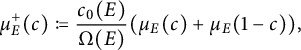
For this exact reason, the modular symbols $ \mu _E(c) $
can be normalized to be integers. More precisely, for an elliptic curve
$ \mu _E(c) $
can be normalized to be integers. More precisely, for an elliptic curve $ E $
of conductor
$ E $
of conductor $ N $
with normalized cuspidal eigenform
$ N $
with normalized cuspidal eigenform $ f_E \in S_2(N) $
, define the normalized modular symbol
$ f_E \in S_2(N) $
, define the normalized modular symbol
which is now an integer. The integrality of $ \mathscr {L}(E) $
is now a formal consequence of the action of Hecke operators on the space of modular symbols.
$ \mathscr {L}(E) $
is now a formal consequence of the action of Hecke operators on the space of modular symbols.
Proposition 3.3 Let $ E $
be an elliptic curve of conductor
$ E $
be an elliptic curve of conductor $ N $
. Let
$ N $
. Let $ v $
be an odd prime such that
$ v $
be an odd prime such that $ v \nmid N $
. Then
$ v \nmid N $
. Then
 $$ \begin{align*}c_0(E)\mathscr{L}(E)\#E(\mathbb{F}_v) = \sum_{a = 1}^{\lfloor\tfrac{v - 1}{2}\rfloor} \mu_E^+(a / v).\end{align*} $$
In particular, both sides lie in $ \mathbb {Z} $
.
$ \mathbb {Z} $
.
Proof The first statement is precisely the action of Hecke operators on the space of modular symbols [Reference Manin22, Theorem 4.2] up to a factor of $ c_0(E)^{-1}\Omega (E) $
. Integrality of both sides then follows immediately from Lemma 3.1 and the first statement.
$ c_0(E)^{-1}\Omega (E) $
. Integrality of both sides then follows immediately from Lemma 3.1 and the first statement.
Remark 3.4 The assumption that $ v \nmid N $
is crucial, and removing this may cause integrality to fail, such as for the elliptic curve 11a1 where
$ v \nmid N $
is crucial, and removing this may cause integrality to fail, such as for the elliptic curve 11a1 where $ c_0(E) = 1 $
and
$ c_0(E) = 1 $
and $ \mathscr {L}(E) = \tfrac {1}{5} $
, but
$ \mathscr {L}(E) = \tfrac {1}{5} $
, but $\#E(\mathbb{F}_{11}) = 11$
.
$\#E(\mathbb{F}_{11}) = 11$
.
The same argument can be adapted for $ \mathscr {L}(E, \chi ) $
using Birch’s formula.
$ \mathscr {L}(E, \chi ) $
using Birch’s formula.
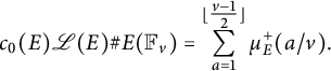
Proposition 3.5 Let $ E $
be an elliptic curve of conductor
$ E $
be an elliptic curve of conductor $ N $
. Let
$ N $
. Let $ \chi $
be a character of order
$ \chi $
be a character of order $ q $
and odd prime conductor
$ q $
and odd prime conductor $ p \nmid N $
. Then
$ p \nmid N $
. Then
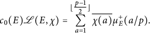 $$ \begin{align*}c_0(E)\mathscr{L}(E, \chi) = \sum_{a = 1}^{\lfloor\tfrac{p - 1}{2}\rfloor} \overline{\chi(a)}\mu_E^+(a / p).\end{align*} $$
In particular, both sides lie in $ \mathbb {Z}[\zeta _q] $
. Furthermore, if
$ \mathbb {Z}[\zeta _q] $
. Furthermore, if $ c_1(E) = 1 $
, then
$ c_1(E) = 1 $
, then $ \mathscr {L}(E, \chi ) \in \mathbb {Z}[\zeta _q] $
.
$ \mathscr {L}(E, \chi ) \in \mathbb {Z}[\zeta _q] $
.
Proof This is identical to the proof by Wiersema–Wuthrich [Reference Wiersema and Wuthrich33, Proposition 7], noting that the automorphic and motivic definitions of $ \mathscr {L}(E, \chi ) $
agree under the assumption that
$ \mathscr {L}(E, \chi ) $
agree under the assumption that $ p \nmid N $
[Reference Wiersema and Wuthrich33, Lemma 18]. Integrality of both sides then follows immediately from Lemma 3.1 and the first statement. The final statement is an analogous argument with
$ p \nmid N $
[Reference Wiersema and Wuthrich33, Lemma 18]. Integrality of both sides then follows immediately from Lemma 3.1 and the first statement. The final statement is an analogous argument with $ c_1(E) $
also given by Wiersema–Wuthrich [Reference Wiersema and Wuthrich33, Proposition 8].
$ c_1(E) $
also given by Wiersema–Wuthrich [Reference Wiersema and Wuthrich33, Proposition 8].
Remark 3.6 The assumption that $ p \nmid N $
can be weakened slightly to
$ p \nmid N $
can be weakened slightly to $ p^2 \nmid N $
for the first two statements [Reference Wiersema and Wuthrich33, Proposition 7]. However, removing this completely may cause integrality to fail, such as for the elliptic curve 50b1 satisfying
$ p^2 \nmid N $
for the first two statements [Reference Wiersema and Wuthrich33, Proposition 7]. However, removing this completely may cause integrality to fail, such as for the elliptic curve 50b1 satisfying $ c_0(E) = 1 $
and the unique quadratic character of conductor
$ c_0(E) = 1 $
and the unique quadratic character of conductor $ 5 $
, where
$ 5 $
, where $ \mathscr {L}(E, \chi ) = \tfrac {1}{3} $
.
$ \mathscr {L}(E, \chi ) = \tfrac {1}{3} $
.
Now observe that the right hand sides of Propositions 3.3 and 3.5 are highly similar. More precisely, since $ \overline {\chi (a)} \equiv 1\ \mod (1 - \zeta _q) $
except when
$ \overline {\chi (a)} \equiv 1\ \mod (1 - \zeta _q) $
except when $ \ell \mid a $
, the right hand sides are congruent modulo
$ \ell \mid a $
, the right hand sides are congruent modulo $ (1 - \zeta _q) $
. This is summarized in the following result, which will be the main tool behind much of the rest of the article.
$ (1 - \zeta _q) $
. This is summarized in the following result, which will be the main tool behind much of the rest of the article.
Corollary 3.7 Let $ E $
be an elliptic curve of conductor
$ E $
be an elliptic curve of conductor $ N $
. Let
$ N $
. Let $ \chi $
be a character of order
$ \chi $
be a character of order $ q $
and odd prime conductor
$ q $
and odd prime conductor $ p \nmid N $
. Then
$ p \nmid N $
. Then
 $$ \begin{align*}c_0(E)\mathscr{L}(E, \chi) \equiv -c_0(E)\mathscr{L}(E)\#E(\mathbb{F}_p) \quad\mod (1 - \zeta_q).\end{align*} $$
Furthermore, if $ q \nmid c_0(E) $
, then
$ q \nmid c_0(E) $
, then
 $$ \begin{align*}\mathscr{L}(E, \chi) \equiv -\mathscr{L}(E)\#E(\mathbb{F}_p) \quad\mod (1 - \zeta_q),\end{align*} $$
where the denominators of both sides are inverted modulo $ (1 - \zeta _q) $
.
$ (1 - \zeta _q) $
.
Remark 3.8 Without considering the factor of $ c_0(E) $
, both integrality results and the congruence easily fail in trivial ways, but the assumption that
$ c_0(E) $
, both integrality results and the congruence easily fail in trivial ways, but the assumption that $ q \nmid c_0(E) $
is a relatively mild one, since
$ q \nmid c_0(E) $
is a relatively mild one, since $ c_0(E) \ne 1 $
seems to be relatively rare.
$ c_0(E) \ne 1 $
seems to be relatively rare.
Remark 3.9 Modified twisted L-values $ \mathscr {L}(E, \chi ) $
are Galois equivariant as predicted by Deligne’s period conjecture [Reference Bouganis and Dokchitser4, Theorem 2.7], in the sense that
$ \mathscr {L}(E, \chi ) $
are Galois equivariant as predicted by Deligne’s period conjecture [Reference Bouganis and Dokchitser4, Theorem 2.7], in the sense that $ \mathscr {L}(E, \sigma \circ \chi ) = \sigma (\mathscr {L}(E, \chi )) $
for any
$ \mathscr {L}(E, \sigma \circ \chi ) = \sigma (\mathscr {L}(E, \chi )) $
for any $ \sigma \in \operatorname {Gal}(\mathbb {Q}(\zeta _q) / \mathbb {Q}) $
. With this property,
$ \sigma \in \operatorname {Gal}(\mathbb {Q}(\zeta _q) / \mathbb {Q}) $
. With this property, $ \mathscr {L}(E) $
can be expressed in terms of the sum of
$ \mathscr {L}(E) $
can be expressed in terms of the sum of $ \mathscr {L}(E, \chi ) $
for all characters
$ \mathscr {L}(E, \chi ) $
for all characters $ \chi $
of a given conductor and order. For instance, when
$ \chi $
of a given conductor and order. For instance, when $ \chi $
is a cubic character of conductor
$ \chi $
is a cubic character of conductor $ p $
,
$ p $
,
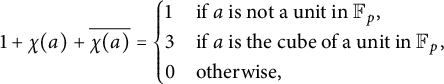 $$ \begin{align*}1 + \chi(a) + \overline{\chi(a)} = \begin{cases} 1 & \text{if} \ a \ \text{is not a unit in} \ \mathbb{F}_p, \\ 3 & \text{if} \ a \ \text{is the cube of a unit in} \ \mathbb{F}_p, \\ 0 & \text{otherwise}, \end{cases} \end{align*} $$
so that the identities in Propositions 3.3 and 3.5 combine to yield
 $$ \begin{align*}c_0(E)\mathscr{L}(E, \chi) + c_0(E)\mathscr{L}(E, \overline{\chi}) + c_0(E)\mathscr{L}(E)\#E(\mathbb{F}_p) = 3\sum_a \mu_E^+(a / p),\end{align*} $$
where the sum runs over the cubic residues $ a $
in
$ a $
in $ \mathbb {F}_p $
such that
$ \mathbb {F}_p $
such that $ 1 \le a \le \lfloor \tfrac {p - 1}{2}\rfloor $
. By Galois equivariance, the first two terms combine to
$ 1 \le a \le \lfloor \tfrac {p - 1}{2}\rfloor $
. By Galois equivariance, the first two terms combine to $ 2c_0(E)\Re (\mathscr {L}(E, \chi )) $
, so that this expresses
$ 2c_0(E)\Re (\mathscr {L}(E, \chi )) $
, so that this expresses $ \Re (\mathscr {L}(E, \chi )) $
in terms of
$ \Re (\mathscr {L}(E, \chi )) $
in terms of $ \mathscr {L}(E) $
up to a few error terms consisting of modular symbols. By reducing modulo
$ \mathscr {L}(E) $
up to a few error terms consisting of modular symbols. By reducing modulo $ 3 $
, this recovers the congruence in Corollary 3.7, but also shows that the congruence would not a priori hold modulo
$ 3 $
, this recovers the congruence in Corollary 3.7, but also shows that the congruence would not a priori hold modulo $ 9 $
, unless the modular symbols
$ 9 $
, unless the modular symbols $ \mu _E^+(a / p) $
for each cubic residue
$ \mu _E^+(a / p) $
for each cubic residue $ a $
in
$ a $
in $ \mathbb {F}_p $
sum to a multiple of
$ \mathbb {F}_p $
sum to a multiple of $ 3 $
.
$ 3 $
.
4 Denominators of L-values
This section proves a few results on the $ \ell $
-adic valuations of denominators of modified L-values, where
$ \ell $
-adic valuations of denominators of modified L-values, where $ \ell $
is an odd prime, which may be of independent interest. Since
$ \ell $
is an odd prime, which may be of independent interest. Since $ c_0(E)\mathscr {L}(E)\#E(\mathbb {F}_v) $
is integral, the
$ c_0(E)\mathscr {L}(E)\#E(\mathbb {F}_v) $
is integral, the $ \ell $
-adic valuation of the rational number
$ \ell $
-adic valuation of the rational number $ c_0(E)\mathscr {L}(E) $
can be bounded from below by the
$ c_0(E)\mathscr {L}(E) $
can be bounded from below by the $ \ell $
-adic valuation of
$ \ell $
-adic valuation of $ \#E(\mathbb {F}_v) $
, which is in turn controlled by
$ \#E(\mathbb {F}_v) $
, which is in turn controlled by $ \operatorname {tor}(E) $
in the denominator of
$ \operatorname {tor}(E) $
in the denominator of $ \operatorname {BSD}(E) $
. When
$ \operatorname {BSD}(E) $
. When $ \ell \ne 3 $
, assuming the
$ \ell \ne 3 $
, assuming the $ \ell $
-part of the Birch–Swinnerton-Dyer conjecture, such a lower bound follows from Lorenzini’s result that
$ \ell $
-part of the Birch–Swinnerton-Dyer conjecture, such a lower bound follows from Lorenzini’s result that $ \operatorname {ord}_\ell (\#\operatorname {tor}(E)) \le \operatorname {ord}_\ell (\operatorname {Tam}(E)) $
with finitely many exceptions [Reference Lorenzini20, Proposition 1.1], but the case
$ \operatorname {ord}_\ell (\#\operatorname {tor}(E)) \le \operatorname {ord}_\ell (\operatorname {Tam}(E)) $
with finitely many exceptions [Reference Lorenzini20, Proposition 1.1], but the case $ \ell = 3 $
requires more work.
$ \ell = 3 $
requires more work.
Lemma 4.1 Let $ E $
be an elliptic curve without complex multiplication such that
$ E $
be an elliptic curve without complex multiplication such that $ E(\mathbb {Q}) $
has a point of order
$ E(\mathbb {Q}) $
has a point of order $ 3 $
and that
$ 3 $
and that $ 3 \nmid \operatorname {Tam}(E) $
. Then
$ 3 \nmid \operatorname {Tam}(E) $
. Then $ \operatorname {im}(\overline {\rho _{E, 3}}) $
is the full Borel subgroup.
$ \operatorname {im}(\overline {\rho _{E, 3}}) $
is the full Borel subgroup.
Proof By the assumption that $ E $
has a point of order
$ E $
has a point of order $ 3 $
,
$ 3 $
, $ E $
is isomorphic either to the elliptic curve given by
$ E $
is isomorphic either to the elliptic curve given by $ y^2 + cy = x^3 $
for some cube-free
$ y^2 + cy = x^3 $
for some cube-free $ c \in \mathbb {N} $
, which has complex multiplication by
$ c \in \mathbb {N} $
, which has complex multiplication by $ \mathbb {Z}[\zeta _3] $
, or to the elliptic curve
$ \mathbb {Z}[\zeta _3] $
, or to the elliptic curve $ E_{1, \pm b / a} $
given by
$ E_{1, \pm b / a} $
given by
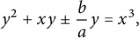 $$ \begin{align*}y^2 + xy \pm \dfrac{b}{a}y = x^3,\end{align*} $$
for some coprime $ a, b \in \mathbb {N} $
[Reference Barrios and Roy1, Proposition 2.4]. If
$ a, b \in \mathbb {N} $
[Reference Barrios and Roy1, Proposition 2.4]. If $ 3 \nmid \operatorname {ord}_v(a) $
for some prime
$ 3 \nmid \operatorname {ord}_v(a) $
for some prime $ v $
, then
$ v $
, then $ 3 \mid \operatorname {Tam}_v(E_{1, \pm b / a}) $
[Reference Barrios and Roy1, Theorem 3.5], which contradicts the assumption that
$ 3 \mid \operatorname {Tam}_v(E_{1, \pm b / a}) $
[Reference Barrios and Roy1, Theorem 3.5], which contradicts the assumption that ${ 3 \nmid \operatorname {Tam}(E) }$
, so that
${ 3 \nmid \operatorname {Tam}(E) }$
, so that $ a = d^3 $
for some
$ a = d^3 $
for some $ d \in \mathbb {N} $
coprime to
$ d \in \mathbb {N} $
coprime to $ b $
. The change of variables
$ b $
. The change of variables $ (x, y) \mapsto (x / d^2, y / d^3) $
yields an isomorphism from
$ (x, y) \mapsto (x / d^2, y / d^3) $
yields an isomorphism from $ E_{1, \pm b / a} $
to the elliptic curve
$ E_{1, \pm b / a} $
to the elliptic curve $ E_{d, \pm b} $
given by
$ E_{d, \pm b} $
given by
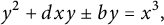 $$ \begin{align*}y^2 + dxy \pm by = x^3,\end{align*} $$
which is now a minimal model and has discriminant $ \Delta = \pm b^3(d^3 - 27b) $
. Now let
$ \Delta = \pm b^3(d^3 - 27b) $
. Now let $ v $
be a prime such that
$ v $
be a prime such that $ v \mid b $
, so that
$ v \mid b $
, so that $ v \mid \Delta $
and
$ v \mid \Delta $
and $ \operatorname {ord}_v(d^3 - 27b) = 0 $
by coprimality. By step
$ \operatorname {ord}_v(d^3 - 27b) = 0 $
by coprimality. By step $ 2 $
of Tate’s algorithm, since
$ 2 $
of Tate’s algorithm, since $ T^2 + dT $
splits in
$ T^2 + dT $
splits in $ \mathbb {F}_v $
, the elliptic curve
$ \mathbb {F}_v $
, the elliptic curve $ E_{d, \pm b} $
has Kodaira symbol
$ E_{d, \pm b} $
has Kodaira symbol $ \mathbf {I}_{\operatorname {ord}_v(\Delta )} $
with split mutiplicative reduction at
$ \mathbf {I}_{\operatorname {ord}_v(\Delta )} $
with split mutiplicative reduction at $ v $
, so that
$ v $
, so that
 $$ \begin{align*}\operatorname{Tam}_v(E) = \operatorname{Tam}_v(E_{d, \pm b}) = \operatorname{ord}_v(\Delta) = 3\operatorname{ord}_v(b),\end{align*} $$
which contradicts the assumption that $ 3 \nmid \operatorname {Tam}(E) $
. This forces
$ 3 \nmid \operatorname {Tam}(E) $
. This forces $ b = 1 $
, but the j-invariant of
$ b = 1 $
, but the j-invariant of $ E_{d, \pm b} = E_{d, \pm 1} $
computes to be
$ E_{d, \pm b} = E_{d, \pm 1} $
computes to be
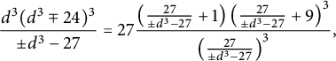 $$ \begin{align*}\dfrac{d^3(d^3 \mp 24)^3}{\pm d^3 - 27} = 27\dfrac{\left(\tfrac{27}{\pm d^3 - 27} + 1\right)\left(\tfrac{27}{\pm d^3 - 27} + 9\right)^3}{\left(\tfrac{27}{\pm d^3 - 27}\right)^3},\end{align*} $$
which implies that $ \operatorname {im}(\overline {\rho _{E, 3}}) $
is the Borel subgroup 3B.1.1 [Reference Zywina35, Theorem 1.2].
$ \operatorname {im}(\overline {\rho _{E, 3}}) $
is the Borel subgroup 3B.1.1 [Reference Zywina35, Theorem 1.2].
Assuming just one direction of the $ 3 $
-part of the Birch–Swinnerton-Dyer conjecture, a clean divisibility result for
$ 3 $
-part of the Birch–Swinnerton-Dyer conjecture, a clean divisibility result for $ \operatorname {BSD}(E) $
can be derived from the integrality of
$ \operatorname {BSD}(E) $
can be derived from the integrality of $ c_0(E)\mathscr {L}(E)\#E(\mathbb {F}_v) $
via a case-by-case analysis on
$ c_0(E)\mathscr {L}(E)\#E(\mathbb {F}_v) $
via a case-by-case analysis on $ \operatorname {im}(\rho _{E, 3}) $
.
$ \operatorname {im}(\rho _{E, 3}) $
.
Proposition 4.2 Let $ E $
be an elliptic curve of conductor
$ E $
be an elliptic curve of conductor $ N $
such that
$ N $
such that $ L(E, 1) \ne 0 $
and that
$ L(E, 1) \ne 0 $
and that $ \operatorname {tor}(E) \cong \mathbb {Z} / 3 $
. Assume further that
$ \operatorname {tor}(E) \cong \mathbb {Z} / 3 $
. Assume further that $ \operatorname {ord}_3(\mathscr {L}(E)) \le \operatorname {ord}_3(\operatorname {BSD}(E)) $
. Then
$ \operatorname {ord}_3(\mathscr {L}(E)) \le \operatorname {ord}_3(\operatorname {BSD}(E)) $
. Then ![]() . In particular, if
. In particular, if $ 3 \nmid c_0(E) $
, then
$ 3 \nmid c_0(E) $
, then $ \operatorname {ord}_3(\operatorname {BSD}(E)) \ge -1 $
.
$ \operatorname {ord}_3(\operatorname {BSD}(E)) \ge -1 $
.
Proof The final statement follows from the first statement, so it suffices to prove the latter. Assume that $ 3 \nmid c_0(E) $
. By Proposition 3.3 and the assumptions,
$ 3 \nmid c_0(E) $
. By Proposition 3.3 and the assumptions,
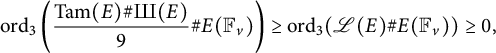
so it suffices to find an odd prime $ v \nmid N $
such that
$ v \nmid N $
such that $ \#E(\mathbb {F}_v) \equiv 3 \ \mod 9 $
. By Chebotarev’s density theorem, this reduces to finding a matrix
$ \#E(\mathbb {F}_v) \equiv 3 \ \mod 9 $
. By Chebotarev’s density theorem, this reduces to finding a matrix $ M \in \operatorname {im}(\overline {\rho _{E, 9}}) $
such that
$ M \in \operatorname {im}(\overline {\rho _{E, 9}}) $
such that $ 1 + \det (M) - \operatorname {tr}(M) = 3 $
. By inspecting the table in Section A.2, such matrices exist for all
$ 1 + \det (M) - \operatorname {tr}(M) = 3 $
. By inspecting the table in Section A.2, such matrices exist for all $ \operatorname {im}(\rho _{E, 3}) $
except for the two
$ \operatorname {im}(\rho _{E, 3}) $
except for the two $ 3 $
-adic Galois images 9.72.0.1 and 9.72.0.5, so these two cases have to be handled separately. If
$ 3 $
-adic Galois images 9.72.0.1 and 9.72.0.5, so these two cases have to be handled separately. If $ \operatorname {im}(\rho _{E, 3}) $
is 9.72.0.1, then
$ \operatorname {im}(\rho _{E, 3}) $
is 9.72.0.1, then $ \operatorname {im}(\overline {\rho _{E, 3}}) $
is 3Cs.1.1 and not 3B.1.1, so Lemma 4.1 implies that
$ \operatorname {im}(\overline {\rho _{E, 3}}) $
is 3Cs.1.1 and not 3B.1.1, so Lemma 4.1 implies that $ 3 \mid \operatorname {Tam}(E) $
. Otherwise
$ 3 \mid \operatorname {Tam}(E) $
. Otherwise $ \operatorname {im}(\rho _{E, 3}) $
is 9.72.0.5, then
$ \operatorname {im}(\rho _{E, 3}) $
is 9.72.0.5, then $ \operatorname {im}(\overline {\rho _{E, 9}}) $
fixes a subspace of the group of
$ \operatorname {im}(\overline {\rho _{E, 9}}) $
fixes a subspace of the group of $ 9 $
-torsion points of
$ 9 $
-torsion points of $ E $
, so that
$ E $
, so that $ E(\mathbb {Q}) \cong \mathbb {Z} / 9 $
, which contradicts the assumption that
$ E(\mathbb {Q}) \cong \mathbb {Z} / 9 $
, which contradicts the assumption that $ E(\mathbb {Q}) \cong \mathbb {Z} / 3 $
.
$ E(\mathbb {Q}) \cong \mathbb {Z} / 3 $
.
Remark 4.3 The conclusion of Proposition 4.2 was already observed by Melistas [Reference Melistas23, Example 3.8], where the elliptic curves 27a3, 27a4, and 54a3 all have $ E(\mathbb {Q}) \cong \mathbb {Z} / 3 $
and
$ E(\mathbb {Q}) \cong \mathbb {Z} / 3 $
and ![]() but
but $ c_0(E) = 3 $
. By the work of Lorenzini, it is generally expected that the factors in
$ c_0(E) = 3 $
. By the work of Lorenzini, it is generally expected that the factors in $ \operatorname {Tam}(E) $
would cancel
$ \operatorname {Tam}(E) $
would cancel $ \#\operatorname {tor}(E) $
, but in this case it is necessary to consider
$ \#\operatorname {tor}(E) $
, but in this case it is necessary to consider ![]() as well, such as in the elliptic curve 1638j3 where
as well, such as in the elliptic curve 1638j3 where $ E(\mathbb {Q}) \cong \mathbb {Z} / 3 $
and
$ E(\mathbb {Q}) \cong \mathbb {Z} / 3 $
and $ c_0(E)\operatorname {Tam}(E) = 1 $
but
$ c_0(E)\operatorname {Tam}(E) = 1 $
but ![]() . Note that the statement is false for
. Note that the statement is false for $ \operatorname {tor}(E) \cong \mathbb {Z} / 3 $
but
$ \operatorname {tor}(E) \cong \mathbb {Z} / 3 $
but $ \operatorname {rk}(E)> 0 $
, such as for the elliptic curve 91b1 where
$ \operatorname {rk}(E)> 0 $
, such as for the elliptic curve 91b1 where ![]() .
.
A lower bound on the $ \ell $
-adic valuation of
$ \ell $
-adic valuation of $ c_0(E)\mathscr {L}(E) $
then follows for any odd prime
$ c_0(E)\mathscr {L}(E) $
then follows for any odd prime $ \ell $
, assuming the
$ \ell $
, assuming the $ \ell $
-part of the Birch–Swinnerton-Dyer conjecture, but when
$ \ell $
-part of the Birch–Swinnerton-Dyer conjecture, but when $ E $
has no rational
$ E $
has no rational $ \ell $
-isogeny the bound is unconditional by simple group theory.
$ \ell $
-isogeny the bound is unconditional by simple group theory.
Theorem 4.4 Let $ E $
be an elliptic curve of conductor
$ E $
be an elliptic curve of conductor $ N $
such that
$ N $
such that $ L(E, 1) \ne 0 $
. Let
$ L(E, 1) \ne 0 $
. Let $ \ell $
be an odd prime.
$ \ell $
be an odd prime.
-
(1) If
$ E $
has no rational
$ \ell $
-isogeny, then
$ \operatorname {ord}_\ell (c_0(E)\mathscr {L}(E)) \ge 0 $
. -
(2) Assume further that
$ \operatorname {ord}_\ell (\mathscr {L}(E)) = \operatorname {ord}_\ell (\operatorname {BSD}(E)) $
. Then
$ \operatorname {ord}_\ell (c_0(E)\mathscr {L}(E)) \ge -1 $
.


Proof For the first statement, by Proposition 3.3, it suffices to find an odd prime $ v \nmid N $
such that
$ v \nmid N $
such that $ \ell \nmid \#E(\mathbb {F}_v) $
. By Chebotarev’s density theorem, this reduces to finding a matrix
$ \ell \nmid \#E(\mathbb {F}_v) $
. By Chebotarev’s density theorem, this reduces to finding a matrix $ M \in \operatorname {im}(\overline {\rho _{E, \ell }}) $
such that
$ M \in \operatorname {im}(\overline {\rho _{E, \ell }}) $
such that $ \operatorname {tr}(M) \ne 1 + \det (M) $
. Suppose otherwise that
$ \operatorname {tr}(M) \ne 1 + \det (M) $
. Suppose otherwise that $ \operatorname {tr}(M) = 1 + \det (M) $
for all matrices
$ \operatorname {tr}(M) = 1 + \det (M) $
for all matrices $ M \in \operatorname {im}(\overline {\rho _{E, \ell }}) $
, so that in particular
$ M \in \operatorname {im}(\overline {\rho _{E, \ell }}) $
, so that in particular $ \operatorname {tr}(M) = 2 $
for all matrices
$ \operatorname {tr}(M) = 2 $
for all matrices $ M \in \operatorname {im}(\overline {\rho _{E, \ell }}) \cap \operatorname {SL}_2(\mathbb {Z} / \ell ) $
. In this case, by inspecting the orders of elements in each conjugacy class of
$ M \in \operatorname {im}(\overline {\rho _{E, \ell }}) \cap \operatorname {SL}_2(\mathbb {Z} / \ell ) $
. In this case, by inspecting the orders of elements in each conjugacy class of $ \operatorname {SL}_2(\mathbb {Z} / \ell ) $
as in Section 2, it is clear that
$ \operatorname {SL}_2(\mathbb {Z} / \ell ) $
as in Section 2, it is clear that $ \operatorname {im}(\overline {\rho _{E, \ell }}) \cap \operatorname {SL}_2(\mathbb {Z} / \ell ) $
is necessarily an
$ \operatorname {im}(\overline {\rho _{E, \ell }}) \cap \operatorname {SL}_2(\mathbb {Z} / \ell ) $
is necessarily an $ \ell $
-group, so that in particular
$ \ell $
-group, so that in particular $ \ell \mid \#\operatorname {im}(\overline {\rho _{E, \ell }}) $
. Then either
$ \ell \mid \#\operatorname {im}(\overline {\rho _{E, \ell }}) $
. Then either $ \operatorname {im}(\overline {\rho _{E, \ell }}) $
is contained in a Borel subgroup of
$ \operatorname {im}(\overline {\rho _{E, \ell }}) $
is contained in a Borel subgroup of $ \operatorname {GL}_2(\mathbb {Z} / \ell ) $
or
$ \operatorname {GL}_2(\mathbb {Z} / \ell ) $
or $ \operatorname {im}(\overline {\rho _{E, \ell }}) $
contains
$ \operatorname {im}(\overline {\rho _{E, \ell }}) $
contains $ \operatorname {SL}_2(\mathbb {Z} / \ell ) $
[Reference Serre26, Proposition 15]. The former contradicts the assumption that
$ \operatorname {SL}_2(\mathbb {Z} / \ell ) $
[Reference Serre26, Proposition 15]. The former contradicts the assumption that $ E $
has no rational
$ E $
has no rational $ \ell $
-isogeny, and the latter is impossible by comparing orders.
$ \ell $
-isogeny, and the latter is impossible by comparing orders.
For the second statement, the assumption that $ \operatorname {ord}_\ell (\mathscr {L}(E)) = \operatorname {ord}_\ell (\operatorname {BSD}(E)) $
reduces the statement to proving that
$ \operatorname {ord}_\ell (\mathscr {L}(E)) = \operatorname {ord}_\ell (\operatorname {BSD}(E)) $
reduces the statement to proving that $ \operatorname {ord}_\ell (c_0(E)\operatorname {BSD}(E)) \ge -1 $
. By Mazur’s torsion theorem, since
$ \operatorname {ord}_\ell (c_0(E)\operatorname {BSD}(E)) \ge -1 $
. By Mazur’s torsion theorem, since $ \ell $
is odd, it suffices to consider
$ \ell $
is odd, it suffices to consider $ \operatorname {tor}(E) $
being one of the eight subgroups
$ \operatorname {tor}(E) $
being one of the eight subgroups
 $$ \begin{align*}\mathbb{Z} / 3, \ \mathbb{Z} / 5, \ \mathbb{Z} / 6, \ \mathbb{Z} / 7, \ \mathbb{Z} / 9, \ \mathbb{Z} / 10, \ \mathbb{Z} / 12, \ \mathbb{Z} / 2 \oplus \mathbb{Z} / 6,\end{align*} $$
If $ E(\mathbb {Q}) \not \cong \mathbb {Z} / 3 $
, then a case-by-case analysis of Lorenzini’s classification yields
$ E(\mathbb {Q}) \not \cong \mathbb {Z} / 3 $
, then a case-by-case analysis of Lorenzini’s classification yields $ \operatorname {ord}_\ell (\operatorname {Tam}(E)) \ge \operatorname {ord}_\ell (\#\operatorname {tor}(E)) $
except for the elliptic curve 11a3 with
$ \operatorname {ord}_\ell (\operatorname {Tam}(E)) \ge \operatorname {ord}_\ell (\#\operatorname {tor}(E)) $
except for the elliptic curve 11a3 with $ \ell = 5 $
, and the elliptic curves 14a4 and 14a6 with
$ \ell = 5 $
, and the elliptic curves 14a4 and 14a6 with $ \ell = 3 $
[Reference Lorenzini20, Proposition 1.1], but these exceptions all have
$ \ell = 3 $
[Reference Lorenzini20, Proposition 1.1], but these exceptions all have $ \operatorname {ord}_\ell (c_0(E)) = 1 $
and
$ \operatorname {ord}_\ell (c_0(E)) = 1 $
and $ \operatorname {ord}_\ell (\operatorname {BSD}(E)) = -2 $
, so that in particular
$ \operatorname {ord}_\ell (\operatorname {BSD}(E)) = -2 $
, so that in particular $ \operatorname {ord}_\ell (c_0(E))\operatorname {BSD}(E)) \ge -1 $
. If
$ \operatorname {ord}_\ell (c_0(E))\operatorname {BSD}(E)) \ge -1 $
. If $ E(\mathbb {Q}) \cong \mathbb {Z} / 3 $
, then Proposition 4.2 implies that
$ E(\mathbb {Q}) \cong \mathbb {Z} / 3 $
, then Proposition 4.2 implies that
as required.
Remark 4.5 The assumption on the $ \ell $
-part of the Birch–Swinnerton-Dyer conjecture in the second statement can be slightly weakened, by only requiring that
$ \ell $
-part of the Birch–Swinnerton-Dyer conjecture in the second statement can be slightly weakened, by only requiring that $ \operatorname {ord}_\ell (\mathscr {L}(E)) \ge \operatorname {ord}_\ell (\operatorname {BSD}(E)) $
for all
$ \operatorname {ord}_\ell (\mathscr {L}(E)) \ge \operatorname {ord}_\ell (\operatorname {BSD}(E)) $
for all $ E $
, except for when
$ E $
, except for when $ \operatorname {im}(\rho _{E, 3}) $
is 9.72.0.1, where the assumption
$ \operatorname {im}(\rho _{E, 3}) $
is 9.72.0.1, where the assumption $ \operatorname {ord}_\ell (\mathscr {L}(E)) \le \operatorname {ord}_\ell (\operatorname {BSD}(E)) $
is also needed to proceed with the argument in Proposition 4.2. In fact, it might also be provable without appealing to the conjecture at all, by finding a matrix
$ \operatorname {ord}_\ell (\mathscr {L}(E)) \le \operatorname {ord}_\ell (\operatorname {BSD}(E)) $
is also needed to proceed with the argument in Proposition 4.2. In fact, it might also be provable without appealing to the conjecture at all, by finding a matrix $ M \in \operatorname {im}(\rho _{E, \ell }) $
such that
$ M \in \operatorname {im}(\rho _{E, \ell }) $
such that $ 1 + \det (M) - \operatorname {tr}(M) \equiv \ell \ \mod \ell ^2 $
along the same lines as the proof of Proposition 4.2. In general, this would need a case-by-case analysis of
$ 1 + \det (M) - \operatorname {tr}(M) \equiv \ell \ \mod \ell ^2 $
along the same lines as the proof of Proposition 4.2. In general, this would need a case-by-case analysis of $ \operatorname {im}(\rho _{E, \ell }) $
for when
$ \operatorname {im}(\rho _{E, \ell }) $
for when $ E $
has no rational
$ E $
has no rational $ \ell $
-isogeny for
$ \ell $
-isogeny for $ \ell> 3 $
, whose classification remains incomplete at present.
$ \ell> 3 $
, whose classification remains incomplete at present.
The following is another easy result on the $ \ell $
-adic valuation of
$ \ell $
-adic valuation of $ \mathscr {L}(E)\#E(\mathbb {F}_v) $
. The factors arising from the denominator of the rational number
$ \mathscr {L}(E)\#E(\mathbb {F}_v) $
. The factors arising from the denominator of the rational number $ \mathscr {L}(E)\#E(\mathbb {F}_v) $
could a priori cancel the factors appearing in
$ \mathscr {L}(E)\#E(\mathbb {F}_v) $
could a priori cancel the factors appearing in $ c_0(E) $
, but the congruence of L-values says that this should not happen, assuming Stevens’s conjecture that
$ c_0(E) $
, but the congruence of L-values says that this should not happen, assuming Stevens’s conjecture that $ c_1(E) = 1 $
.
$ c_1(E) = 1 $
.
Proposition 4.6 Let $ E $
be an elliptic curve of conductor
$ E $
be an elliptic curve of conductor $ N $
such that
$ N $
such that $ {L(E, 1) \ne 0} $
. Let
$ {L(E, 1) \ne 0} $
. Let $ v $
and
$ v $
and $ \ell $
be odd primes such that
$ \ell $
be odd primes such that $ v \nmid N $
and that
$ v \nmid N $
and that $ v \equiv 1 \ \mod \ell $
. Assume further that
$ v \equiv 1 \ \mod \ell $
. Assume further that $ {c_1(E) = 1 }$
. Then
$ {c_1(E) = 1 }$
. Then $ \ell \nmid c_0(E)\mathscr {L}(E)\#E(\mathbb {F}_v) $
if and only if
$ \ell \nmid c_0(E)\mathscr {L}(E)\#E(\mathbb {F}_v) $
if and only if $ \ell \nmid c_0(E) $
and
$ \ell \nmid c_0(E) $
and $ \operatorname {ord}_\ell (\mathscr {L}(E)\#E(\mathbb {F}_v)) = 0 $
.
$ \operatorname {ord}_\ell (\mathscr {L}(E)\#E(\mathbb {F}_v)) = 0 $
.
Proof Assume that $ \ell \nmid c_0(E)\mathscr {L}(E)\#E(\mathbb {F}_v) $
but
$ \ell \nmid c_0(E)\mathscr {L}(E)\#E(\mathbb {F}_v) $
but $ \ell \mid c_0(E) $
. By the assumption that
$ \ell \mid c_0(E) $
. By the assumption that $ c_1(E) = 1 $
, Proposition 3.5 says that
$ c_1(E) = 1 $
, Proposition 3.5 says that $ \mathscr {L}(E, \chi ) \in \mathbb {Z}[\zeta _\ell ] $
for any character
$ \mathscr {L}(E, \chi ) \in \mathbb {Z}[\zeta _\ell ] $
for any character $ \chi $
of conductor
$ \chi $
of conductor $ v $
and order
$ v $
and order $ \ell $
, so that
$ \ell $
, so that $ c_0(E)\mathscr {L}(E, \chi ) \equiv 0 \ \mod (1 - \zeta _\ell ) $
, which contradicts
$ c_0(E)\mathscr {L}(E, \chi ) \equiv 0 \ \mod (1 - \zeta _\ell ) $
, which contradicts $ \ell \nmid c_0(E)\mathscr {L}(E)\#E(\mathbb {F}_v) $
by Corollary 3.7. Thus
$ \ell \nmid c_0(E)\mathscr {L}(E)\#E(\mathbb {F}_v) $
by Corollary 3.7. Thus $ \ell \nmid c_0(E) $
, so that
$ \ell \nmid c_0(E) $
, so that $ \operatorname {ord}_\ell (\mathscr {L}(E)\#E(\mathbb {F}_v)) = 0 $
also follows, while the converse is immediate noting that
$ \operatorname {ord}_\ell (\mathscr {L}(E)\#E(\mathbb {F}_v)) = 0 $
also follows, while the converse is immediate noting that $ \mathscr {L}(E) \ne 0 $
.
$ \mathscr {L}(E) \ne 0 $
.
Remark 4.7 Assuming Stevens’s conjecture, Proposition 4.6 yields an immediate proof that $ \mathscr {L}(E)\#E(\mathbb {F}_v) $
is integral at
$ \mathscr {L}(E)\#E(\mathbb {F}_v) $
is integral at $ \ell $
if
$ \ell $
if $ \operatorname {ord}_\ell (c_0(E)) \le 1 $
. This condition seems to hold for all elliptic curves in the LMFDB [32], but a proof remains elusive. On the other hand, assuming the
$ \operatorname {ord}_\ell (c_0(E)) \le 1 $
. This condition seems to hold for all elliptic curves in the LMFDB [32], but a proof remains elusive. On the other hand, assuming the $ \ell $
-part of the Birch–Swinnerton-Dyer conjecture, there might be a direct proof that
$ \ell $
-part of the Birch–Swinnerton-Dyer conjecture, there might be a direct proof that $ \mathscr {L}(E)\#E(\mathbb {F}_v) $
is integral at
$ \mathscr {L}(E)\#E(\mathbb {F}_v) $
is integral at $ \ell $
, by arguing that
$ \ell $
, by arguing that $ 1 + \det (M) - \operatorname {tr}(M) $
cancels
$ 1 + \det (M) - \operatorname {tr}(M) $
cancels $ \#\operatorname {tor}(E)^2 $
for every matrix
$ \#\operatorname {tor}(E)^2 $
for every matrix $ M $
lying in every possible
$ M $
lying in every possible $ \operatorname {im}(\rho _{E, \ell }) $
.
$ \operatorname {im}(\rho _{E, \ell }) $
.
5 Units of twisted L-values
Under the standard arithmetic conjectures, Dokchitser–Evans–Wiersema computed the norm of $ \mathscr {L}(E, \chi ) $
in terms of
$ \mathscr {L}(E, \chi ) $
in terms of $ \operatorname {BSD}(E) $
and
$ \operatorname {BSD}(E) $
and $ \operatorname {BSD}(E / K) $
, where
$ \operatorname {BSD}(E / K) $
, where $ K $
is the degree
$ K $
is the degree $ q $
subfield of
$ q $
subfield of $ \mathbb {Q}(\zeta _p) $
cut out by the kernel of
$ \mathbb {Q}(\zeta _p) $
cut out by the kernel of $ \chi $
[Reference Dokchitser, Evans and Wiersema12, Theorem 38]. Some of their main results can be summarized in the notation of this article as follows.
$ \chi $
[Reference Dokchitser, Evans and Wiersema12, Theorem 38]. Some of their main results can be summarized in the notation of this article as follows.
Proposition 5.1 Let $ E $
be an elliptic curve of conductor
$ E $
be an elliptic curve of conductor $ N $
such that
$ N $
such that $ {L(E, 1) \ne 0} $
. Let
$ {L(E, 1) \ne 0} $
. Let $ \chi $
be a character of odd prime conductor
$ \chi $
be a character of odd prime conductor $ p \nmid N $
and odd prime order
$ p \nmid N $
and odd prime order $ q \nmid c_0(E)\operatorname {BSD}(E)\#E(\mathbb {F}_p) $
. Assume further that
$ q \nmid c_0(E)\operatorname {BSD}(E)\#E(\mathbb {F}_p) $
. Assume further that $ c_1(E) = 1 $
, and that
$ c_1(E) = 1 $
, and that $ \mathscr {L}(E) = \operatorname {BSD}(E) $
and
$ \mathscr {L}(E) = \operatorname {BSD}(E) $
and $ \mathscr {L}(E / K) = \operatorname {BSD}(E / K) $
.
$ \mathscr {L}(E / K) = \operatorname {BSD}(E / K) $
.
-
(1) The cyclotomic integer
$ \mathscr {L}(E, \chi ) \in \mathbb {Z}[\zeta _q] $
has norm and it generates an ideal that is invariant under complex conjugation.
$$ \begin{align*}\operatorname{Nm}_q(\mathscr{L}(E, \chi)) = \pm\dfrac{\operatorname{BSD}(E / K)}{\operatorname{BSD}(E)},\end{align*} $$
-
(2) The real cyclotomic integer
$ \mathscr {L}(E, \chi )\zeta \in \mathbb {Z}[\zeta _q]^+ $
has norm where the positive rational number
$$ \begin{align*}\operatorname{Nm}_q^+(\mathscr{L}(E, \chi)\zeta) = \pm B,\end{align*} $$
$ B \in \mathbb {Q}^\times $
is the positive square root of the positive rational square
$ \operatorname {BSD}(E / K) / \operatorname {BSD}(E) \in (\mathbb {Q}^\times )^2 $
, and .


In particular, if $ B = 1 $
, then there is a unit
$ B = 1 $
, then there is a unit $ u \in \mathbb {Z}[\zeta _q]^+ $
such that
$ u \in \mathbb {Z}[\zeta _q]^+ $
such that $ \mathscr {L}(E, \chi ) = u\zeta ^{-1} $
.
$ \mathscr {L}(E, \chi ) = u\zeta ^{-1} $
.
Proof By Proposition 4.6, under the arithmetic conjectures, the assumption that $ q \nmid c_0(E)\operatorname {BSD}(E)\#E(\mathbb {F}_p) $
reduces to
$ q \nmid c_0(E)\operatorname {BSD}(E)\#E(\mathbb {F}_p) $
reduces to $ q \nmid c_0(E) $
and
$ q \nmid c_0(E) $
and $ \operatorname {ord}_q(\mathscr {L}(E)\#E(\mathbb {F}_p)) = 0 $
. In particular
$ \operatorname {ord}_q(\mathscr {L}(E)\#E(\mathbb {F}_p)) = 0 $
. In particular $ L(E, 1) \ne 0 $
, and moreover
$ L(E, 1) \ne 0 $
, and moreover $ \operatorname {ord}_q(\mathscr {L}(E, \chi )) = 0 $
by Corollary 3.7, so that
$ \operatorname {ord}_q(\mathscr {L}(E, \chi )) = 0 $
by Corollary 3.7, so that $ L(E, \chi , 1) \ne 0 $
as well. This verifies the assumptions of a result by Dokchitser–Evans–Wiersema [Reference Dokchitser, Evans and Wiersema12, Theorem 13(5)–Theorem 13(12)], and is a restatement.
$ L(E, \chi , 1) \ne 0 $
as well. This verifies the assumptions of a result by Dokchitser–Evans–Wiersema [Reference Dokchitser, Evans and Wiersema12, Theorem 13(5)–Theorem 13(12)], and is a restatement.
In ideal-theoretic language, Proposition 5.1.1 predicts that the ideal $ I $
of
$ I $
of $ \mathbb {Z}[\zeta _q] $
generated by
$ \mathbb {Z}[\zeta _q] $
generated by $ \mathscr {L}(E, \chi ) $
has norm equal to the nonzero positive rational number
$ \mathscr {L}(E, \chi ) $
has norm equal to the nonzero positive rational number $ \operatorname {BSD}(E / K) / \operatorname {BSD}(E) $
, and Proposition 5.1.2 says that this rational number is the square of a positive rational number
$ \operatorname {BSD}(E / K) / \operatorname {BSD}(E) $
, and Proposition 5.1.2 says that this rational number is the square of a positive rational number $ B $
equal to the norm of the ideal of
$ B $
equal to the norm of the ideal of $ \mathbb {Z}[\zeta _q]^+ $
generated
$ \mathbb {Z}[\zeta _q]^+ $
generated $ \mathscr {L}(E, \chi )\zeta $
. Thus there are only finitely many possibilities for the prime ideal factorization of
$ \mathscr {L}(E, \chi )\zeta $
. Thus there are only finitely many possibilities for the prime ideal factorization of $ I $
, and the fact that
$ I $
, and the fact that $ I $
is invariant under complex conjugation narrows down the possibilities further. The precise ideal factorization can then be recovered from the
$ I $
is invariant under complex conjugation narrows down the possibilities further. The precise ideal factorization can then be recovered from the $ \operatorname {Gal}(K / \mathbb {Q}) $
-module structure of
$ \operatorname {Gal}(K / \mathbb {Q}) $
-module structure of ![]() [Reference Burns and Castillo5, Remark 7.4], such as in the case of
[Reference Burns and Castillo5, Remark 7.4], such as in the case of $ \operatorname {Gal}(K / \mathbb {Q}) \cong \mathbb {Z} / 5 $
explored by Maistret–Shukla [Reference Maistret and Shukla21, Theorem 1.4].
$ \operatorname {Gal}(K / \mathbb {Q}) \cong \mathbb {Z} / 5 $
explored by Maistret–Shukla [Reference Maistret and Shukla21, Theorem 1.4].
Assuming that $ I $
has been computed as an ideal of
$ I $
has been computed as an ideal of $ \mathbb {Z}[\zeta _q] $
, any generator of
$ \mathbb {Z}[\zeta _q] $
, any generator of $ I $
is only equal to the actual value of
$ I $
is only equal to the actual value of $ \mathscr {L}(E, \chi ) $
up to a unit
$ \mathscr {L}(E, \chi ) $
up to a unit $ u \in \mathbb {Z}[\zeta _q] $
. Proposition 5.1.2 refines this prediction slightly by adding a condition on the norm of
$ u \in \mathbb {Z}[\zeta _q] $
. Proposition 5.1.2 refines this prediction slightly by adding a condition on the norm of $ \mathscr {L}(E, \chi )\zeta $
, which determines the actual value of
$ \mathscr {L}(E, \chi )\zeta $
, which determines the actual value of $ \mathscr {L}(E, \chi ) $
up to a unit
$ \mathscr {L}(E, \chi ) $
up to a unit $ u \in \mathbb {Z}[\zeta _q]^+ $
. In the special case of
$ u \in \mathbb {Z}[\zeta _q]^+ $
. In the special case of $ q = 3 $
, this is still ambiguous up to a sign, since the units of
$ q = 3 $
, this is still ambiguous up to a sign, since the units of $ \mathbb {Z}[\zeta _3]^+ = \mathbb {Z} $
are
$ \mathbb {Z}[\zeta _3]^+ = \mathbb {Z} $
are $ \pm 1 $
. Corollary 3.7 comes into the picture by pinning down the sign in terms of
$ \pm 1 $
. Corollary 3.7 comes into the picture by pinning down the sign in terms of $ \#E(\mathbb {F}_p) $
.
$ \#E(\mathbb {F}_p) $
.
Corollary 5.2 Let $ E $
be an elliptic curve of conductor
$ E $
be an elliptic curve of conductor $ N $
such that
$ N $
such that $ L(E, 1) \ne 0 $
. Let
$ L(E, 1) \ne 0 $
. Let $ \chi $
be a cubic character of odd prime conductor
$ \chi $
be a cubic character of odd prime conductor $ p \nmid N $
such that
$ p \nmid N $
such that $ 3 \nmid c_0(E)\operatorname {BSD}(E)\#E(\mathbb {F}_p) $
. Assume further that
$ 3 \nmid c_0(E)\operatorname {BSD}(E)\#E(\mathbb {F}_p) $
. Assume further that $ c_1(E) = 1 $
, and that
$ c_1(E) = 1 $
, and that $ \mathscr {L}(E) = \operatorname {BSD}(E) $
and
$ \mathscr {L}(E) = \operatorname {BSD}(E) $
and $ \mathscr {L}(E / K) = \operatorname {BSD}(E / K) $
. Then
$ \mathscr {L}(E / K) = \operatorname {BSD}(E / K) $
. Then
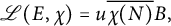 $$ \begin{align*}\mathscr{L}(E, \chi) = u\overline{\chi(N)}B,\end{align*} $$
where the positive rational number $ B \in \mathbb {Q}^\times $
is the positive square root of the positive rational square
$ B \in \mathbb {Q}^\times $
is the positive square root of the positive rational square $ \operatorname {BSD}(E / K) / \operatorname {BSD}(E) \in (\mathbb {Q}^\times )^2 $
, and the sign
$ \operatorname {BSD}(E / K) / \operatorname {BSD}(E) \in (\mathbb {Q}^\times )^2 $
, and the sign $ u = \pm 1 $
is such that
$ u = \pm 1 $
is such that
 $$ \begin{align*}u \equiv -\#E(\mathbb{F}_p)\operatorname{BSD}(E)B^{-1} \quad\mod 3.\end{align*} $$
This follows immediately from Corollary 3.7 and Proposition 5.1. Corollary 5.2 clarifies much of the phenomena observed by Dokchitser–Evans–Wiersema [Reference Dokchitser, Evans and Wiersema12, Example 45], where they gave many pairs of examples of arithmetically similar elliptic curves $ E_1 $
and
$ E_1 $
and $ E_2 $
with
$ E_2 $
with $ \mathscr {L}(E_1, \chi ) \ne \mathscr {L}(E_2, \chi ) $
for a few cubic characters
$ \mathscr {L}(E_1, \chi ) \ne \mathscr {L}(E_2, \chi ) $
for a few cubic characters $ \chi $
, in the sense that
$ \chi $
, in the sense that $ \mathscr {L}(E_1, \chi ) \ne \mathscr {L}(E_2, \chi ) $
precisely because
$ \mathscr {L}(E_1, \chi ) \ne \mathscr {L}(E_2, \chi ) $
precisely because $ \#E_1(\mathbb {F}_p) \not \equiv \#E_2(\mathbb {F}_p) \ \mod 3 $
.
$ \#E_1(\mathbb {F}_p) \not \equiv \#E_2(\mathbb {F}_p) \ \mod 3 $
.
Example 5.3 Let $ E_1 $
and
$ E_1 $
and $ E_2 $
be the elliptic curves 1356d1 and 1356f1, and let
$ E_2 $
be the elliptic curves 1356d1 and 1356f1, and let $ \chi $
be the cubic character of conductor
$ \chi $
be the cubic character of conductor $ 7 $
given by
$ 7 $
given by $ \chi (3) = \zeta _3^2 $
. Then
$ \chi (3) = \zeta _3^2 $
. Then $ c_0(E_i) = \operatorname {BSD}(E_i) = \operatorname {BSD}(E_i / K) = 1 $
for
$ c_0(E_i) = \operatorname {BSD}(E_i) = \operatorname {BSD}(E_i / K) = 1 $
for $ i \in \{1, 2\} $
, so Proposition 5.1 implies that
$ i \in \{1, 2\} $
, so Proposition 5.1 implies that $ \mathscr {L}(E_i, \chi ) = \pm \overline {\chi (1356)} = \pm \zeta _3^2 $
, but it was a priori unclear why
$ \mathscr {L}(E_i, \chi ) = \pm \overline {\chi (1356)} = \pm \zeta _3^2 $
, but it was a priori unclear why $ \mathscr {L}(E_1, \chi ) = \zeta _3^2 $
and
$ \mathscr {L}(E_1, \chi ) = \zeta _3^2 $
and $ \mathscr {L}(E_2, \chi ) = -\zeta _3^2 $
. Corollary 5.2 explains this by requiring that this sign agrees with
$ \mathscr {L}(E_2, \chi ) = -\zeta _3^2 $
. Corollary 5.2 explains this by requiring that this sign agrees with $ -\#E_i(\mathbb {F}_7) $
modulo
$ -\#E_i(\mathbb {F}_7) $
modulo $ 3 $
, and in this case
$ 3 $
, and in this case $ \#E_1(\mathbb {F}_7) = 11 $
and
$ \#E_1(\mathbb {F}_7) = 11 $
and $ \#E_2(\mathbb {F}_7) = 7 $
, which are distinct modulo
$ \#E_2(\mathbb {F}_7) = 7 $
, which are distinct modulo $ 3 $
. They provided other examples satisfying
$ 3 $
. They provided other examples satisfying $ c_0(E) = \operatorname {BSD}(E) = \operatorname {BSD}(E / K) = 1 $
with different
$ c_0(E) = \operatorname {BSD}(E) = \operatorname {BSD}(E / K) = 1 $
with different $ \mathscr {L}(E, \chi ) $
for a few different cubic characters
$ \mathscr {L}(E, \chi ) $
for a few different cubic characters $ \chi $
, and they can all be explained similarly. The values of
$ \chi $
, and they can all be explained similarly. The values of $ \mathscr {L}(E, \chi ) $
for the above character are tabulated as follows.
$ \mathscr {L}(E, \chi ) $
for the above character are tabulated as follows.
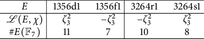
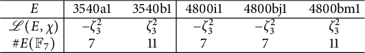
When $ q> 3 $
but
$ q> 3 $
but $ \operatorname {BSD}(E) = \operatorname {BSD}(E / K) $
, Proposition 5.1 says that
$ \operatorname {BSD}(E) = \operatorname {BSD}(E / K) $
, Proposition 5.1 says that $ \mathscr {L}(E, \chi ) $
is a unit in
$ \mathscr {L}(E, \chi ) $
is a unit in $ \mathbb {Z}[\zeta _q] $
, and Corollary 3.7 places a congruence on this unit in terms of
$ \mathbb {Z}[\zeta _q] $
, and Corollary 3.7 places a congruence on this unit in terms of $ \#E(\mathbb {F}_p) $
.
$ \#E(\mathbb {F}_p) $
.
Corollary 5.4 Let $ E $
be an elliptic curve of conductor
$ E $
be an elliptic curve of conductor $ N $
such that
$ N $
such that $ L(E, 1) \ne 0 $
. Let
$ L(E, 1) \ne 0 $
. Let $ \chi $
be a character of odd prime conductor
$ \chi $
be a character of odd prime conductor $ p \nmid N $
and odd prime order
$ p \nmid N $
and odd prime order $ q \nmid c_0(E)\operatorname {BSD}(E)\#E(\mathbb {F}_p) $
such that
$ q \nmid c_0(E)\operatorname {BSD}(E)\#E(\mathbb {F}_p) $
such that $ \operatorname {BSD}(E) = \operatorname {BSD}(E / K) $
. Assume further that
$ \operatorname {BSD}(E) = \operatorname {BSD}(E / K) $
. Assume further that $ c_1(E) = 1 $
, and that
$ c_1(E) = 1 $
, and that $ \mathscr {L}(E) = \operatorname {BSD}(E) $
and
$ \mathscr {L}(E) = \operatorname {BSD}(E) $
and $ \mathscr {L}(E / K) = \operatorname {BSD}(E / K) $
. Then
$ \mathscr {L}(E / K) = \operatorname {BSD}(E / K) $
. Then $ \mathscr {L}(E, \chi ) = u $
for some unit
$ \mathscr {L}(E, \chi ) = u $
for some unit $ u \in \mathbb {Z}[\zeta _q] $
such that
$ u \in \mathbb {Z}[\zeta _q] $
such that $ u \equiv -\#E(\mathbb {F}_p)\operatorname {BSD}(E) \ \mod (1 - \zeta _q) $
.
$ u \equiv -\#E(\mathbb {F}_p)\operatorname {BSD}(E) \ \mod (1 - \zeta _q) $
.
Again, this follows immediately from Corollary 3.7 and Proposition 5.1. Corollary 5.4 explains the remaining phenomena observed by Dokchitser–Evans–Wiersema [Reference Dokchitser, Evans and Wiersema12, Example 44], where they gave many pairs of examples of arithmetically trivial elliptic curves $ E_1 $
and
$ E_1 $
and $ E_2 $
with
$ E_2 $
with $ \mathscr {L}(E_1, \chi ) \ne \mathscr {L}(E_2, \chi ) $
for quintic characters
$ \mathscr {L}(E_1, \chi ) \ne \mathscr {L}(E_2, \chi ) $
for quintic characters $ \chi $
, in the sense that
$ \chi $
, in the sense that $ \mathscr {L}(E_1, \chi ) \ne \mathscr {L}(E_2, \chi ) $
precisely because
$ \mathscr {L}(E_1, \chi ) \ne \mathscr {L}(E_2, \chi ) $
precisely because $ \#E_1(\mathbb {F}_p) \not \equiv \#E_2(\mathbb {F}_p) \ \mod 5 $
.
$ \#E_1(\mathbb {F}_p) \not \equiv \#E_2(\mathbb {F}_p) \ \mod 5 $
.
Example 5.5 Let $ E_1 $
and
$ E_1 $
and $ E_2 $
be the elliptic curves 307a1 and 307c1, and let
$ E_2 $
be the elliptic curves 307a1 and 307c1, and let $ \chi $
be the quintic character of conductor
$ \chi $
be the quintic character of conductor $ 11 $
given by
$ 11 $
given by $ \chi (2) = \zeta _5 $
. Then
$ \chi (2) = \zeta _5 $
. Then $ c_0(E_i) = \operatorname {BSD}(E_i) = \operatorname {BSD}(E_i / K) = 1 $
for
$ c_0(E_i) = \operatorname {BSD}(E_i) = \operatorname {BSD}(E_i / K) = 1 $
for $ i \in \{1, 2\} $
, so Proposition 5.1 implies that
$ i \in \{1, 2\} $
, so Proposition 5.1 implies that $ \mathscr {L}(E_i, \chi ) $
is a unit, but it was a priori unclear why
$ \mathscr {L}(E_i, \chi ) $
is a unit, but it was a priori unclear why $ \mathscr {L}(E_1, \chi ) = 1 $
and
$ \mathscr {L}(E_1, \chi ) = 1 $
and $ \mathscr {L}(E_2, \chi ) = \zeta _5u^2 $
, where
$ \mathscr {L}(E_2, \chi ) = \zeta _5u^2 $
, where ![]() . Corollary 5.4 explains this by requiring that
. Corollary 5.4 explains this by requiring that $ \mathscr {L}(E_i, \chi ) \equiv -\#E_i(\mathbb {F}_{11}) \ \mod (1 - \zeta _5) $
, and in this case
$ \mathscr {L}(E_i, \chi ) \equiv -\#E_i(\mathbb {F}_{11}) \ \mod (1 - \zeta _5) $
, and in this case $ \#E_1(\mathbb {F}_{11}) = 9 $
and
$ \#E_1(\mathbb {F}_{11}) = 9 $
and $ \#E_2(\mathbb {F}_{11}) = 16 $
, which are distinct modulo
$ \#E_2(\mathbb {F}_{11}) = 16 $
, which are distinct modulo $ 5 $
. They provided other examples satisfying
$ 5 $
. They provided other examples satisfying $ c_0(E) = \operatorname {BSD}(E) = \operatorname {BSD}(E / K) = 1 $
with different
$ c_0(E) = \operatorname {BSD}(E) = \operatorname {BSD}(E / K) = 1 $
with different $ \mathscr {L}(E, \chi ) $
for this character, and they can all be explained similarly as follows.
$ \mathscr {L}(E, \chi ) $
for this character, and they can all be explained similarly as follows.
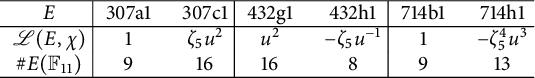
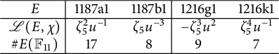
When $ q> 3 $
and
$ q> 3 $
and $ \operatorname {BSD}(E) \ne \operatorname {BSD}(E / K) $
, it is awkward to rephrase Proposition 5.1 to apply Corollary 3.7, but it can be illustrated with an example [Reference Dokchitser, Evans and Wiersema12, Example 46].
$ \operatorname {BSD}(E) \ne \operatorname {BSD}(E / K) $
, it is awkward to rephrase Proposition 5.1 to apply Corollary 3.7, but it can be illustrated with an example [Reference Dokchitser, Evans and Wiersema12, Example 46].
Example 5.6 Let $ E_1 $
and
$ E_1 $
and $ E_2 $
be the elliptic curves 291d1 and 139a1, and let
$ E_2 $
be the elliptic curves 291d1 and 139a1, and let $ \chi $
be the quintic character of conductor
$ \chi $
be the quintic character of conductor $ 31 $
given by
$ 31 $
given by $ \chi (3) = \zeta _5^3 $
. Then
$ \chi (3) = \zeta _5^3 $
. Then $ c_0(E_i) = \operatorname {BSD}(E_i) = 1 $
, but
$ c_0(E_i) = \operatorname {BSD}(E_i) = 1 $
, but $ \operatorname {BSD}(E_i / K) = 11^2 $
for
$ \operatorname {BSD}(E_i / K) = 11^2 $
for $ i \in \{1, 2\} $
, so Proposition 5.1 implies that
$ i \in \{1, 2\} $
, so Proposition 5.1 implies that $ \mathscr {L}(E_i, \chi ) $
generates an ideal of norm
$ \mathscr {L}(E_i, \chi ) $
generates an ideal of norm $ 11^2 $
that is invariant under complex conjugation. By considering the primes above
$ 11^2 $
that is invariant under complex conjugation. By considering the primes above $ 11^2 $
in
$ 11^2 $
in $ \mathbb {Z}[\zeta _5] $
, there are only two such ideals, generated by
$ \mathbb {Z}[\zeta _5] $
, there are only two such ideals, generated by ![]() and
and ![]() , and in fact
, and in fact $ (\mathscr {L}(E_i, \chi )) = (\lambda _i) $
. Assuming this fact, Corollary 3.7 then predicts that
$ (\mathscr {L}(E_i, \chi )) = (\lambda _i) $
. Assuming this fact, Corollary 3.7 then predicts that $ \mathscr {L}(E_i, \chi ) = u_i\lambda _i $
for some units
$ \mathscr {L}(E_i, \chi ) = u_i\lambda _i $
for some units $ u_i \in \mathbb {Z}[\zeta _5] $
such that
$ u_i \in \mathbb {Z}[\zeta _5] $
such that $ 2u_i \equiv -\#E_i(\mathbb {F}_{31}) \ \mod (1 - \zeta _5) $
, and in this case
$ 2u_i \equiv -\#E_i(\mathbb {F}_{31}) \ \mod (1 - \zeta _5) $
, and in this case $ \#E_1(\mathbb {F}_{31}) = 33 \equiv 3 \ \mod 5 $
and
$ \#E_1(\mathbb {F}_{31}) = 33 \equiv 3 \ \mod 5 $
and $ \#E_1(\mathbb {F}_{31}) = 23 \equiv 3 \ \mod 5 $
, so that
$ \#E_1(\mathbb {F}_{31}) = 23 \equiv 3 \ \mod 5 $
, so that $ u_i \equiv 1 \ \mod (1 - \zeta _5) $
. In fact,
$ u_i \equiv 1 \ \mod (1 - \zeta _5) $
. In fact, $ u_1 = \zeta _5^4 $
and
$ u_1 = \zeta _5^4 $
and $ u_2 = \zeta _5^2 - \zeta _5 + 1 $
.
$ u_2 = \zeta _5^2 - \zeta _5 + 1 $
.
Remark 5.7 As this example highlights, in general it is possible for $ \mathscr {L}(E_1, \chi ) \equiv \mathscr {L}(E_2, \chi ) \ \mod (1 - \zeta _q) $
but
$ \mathscr {L}(E_1, \chi ) \equiv \mathscr {L}(E_2, \chi ) \ \mod (1 - \zeta _q) $
but $ \mathscr {L}(E_1, \chi ) \ne \mathscr {L}(E_2, \chi ) $
, even when
$ \mathscr {L}(E_1, \chi ) \ne \mathscr {L}(E_2, \chi ) $
, even when $ c_0(E_i) = \operatorname {BSD}(E_i) \,{=}\, 1 $
, so that a general Birch–Swinnerton-Dyer formula for
$ c_0(E_i) = \operatorname {BSD}(E_i) \,{=}\, 1 $
, so that a general Birch–Swinnerton-Dyer formula for $ \mathscr {L}(E, \chi ) $
remains unlikely even with the factor of
$ \mathscr {L}(E, \chi ) $
remains unlikely even with the factor of $ \#E(\mathbb {F}_p) $
. There are also examples for when
$ \#E(\mathbb {F}_p) $
. There are also examples for when $ E_i $
have the same conductor and minimal discriminant, and furthermore
$ E_i $
have the same conductor and minimal discriminant, and furthermore $ \operatorname {BSD}(E_i / K) = 1 $
, such as for the elliptic curves 544b1 and 544f1 and the quintic character
$ \operatorname {BSD}(E_i / K) = 1 $
, such as for the elliptic curves 544b1 and 544f1 and the quintic character $ \chi $
of conductor
$ \chi $
of conductor $ 11 $
given by
$ 11 $
given by $ \chi (2) = \zeta _5 $
, where
$ \chi (2) = \zeta _5 $
, where $ \mathscr {L}(E_1, \chi ) = -\zeta _5^3 - \zeta _5 $
and
$ \mathscr {L}(E_1, \chi ) = -\zeta _5^3 - \zeta _5 $
and $ \mathscr {L}(E_2, \chi ) = -2\zeta _5^3 - 3\zeta _5^2 - 2\zeta _5 $
. This is the pair of elliptic curves with the smallest conductor satisfying the aforementioned properties but with
$ \mathscr {L}(E_2, \chi ) = -2\zeta _5^3 - 3\zeta _5^2 - 2\zeta _5 $
. This is the pair of elliptic curves with the smallest conductor satisfying the aforementioned properties but with $ \mathscr {L}(E_1, \chi ) \ne \mathscr {L}(E_2, \chi ) $
, but other examples do seem to be rare.
$ \mathscr {L}(E_1, \chi ) \ne \mathscr {L}(E_2, \chi ) $
, but other examples do seem to be rare.
6 Residual densities of twisted L-values
For a fixed elliptic curve $ E $
of conductor
$ E $
of conductor $ N $
, a natural problem is to determine the asymptotic distribution of
$ N $
, a natural problem is to determine the asymptotic distribution of $ \mathscr {L}(E, \chi ) $
, as
$ \mathscr {L}(E, \chi ) $
, as $ \chi $
varies over characters of some fixed prime order
$ \chi $
varies over characters of some fixed prime order $ q $
but of arbitrarily high odd prime conductor
$ q $
but of arbitrarily high odd prime conductor $ p \nmid N $
. However, for each such
$ p \nmid N $
. However, for each such $ p $
, there are
$ p $
, there are $ q - 1 $
characters
$ q - 1 $
characters $ \chi $
of conductor
$ \chi $
of conductor $ p $
and order
$ p $
and order $ q $
, giving rise to
$ q $
, giving rise to $ q - 1 $
conjugates of
$ q - 1 $
conjugates of $ \mathscr {L}(E, \chi ) $
, so that a uniform choice of
$ \mathscr {L}(E, \chi ) $
, so that a uniform choice of $ \chi $
for each
$ \chi $
for each $ p $
has to be made for any meaningful analysis. One solution is to observe that the residue class of
$ p $
has to be made for any meaningful analysis. One solution is to observe that the residue class of $ \mathscr {L}(E, \chi ) $
modulo
$ \mathscr {L}(E, \chi ) $
modulo $ (1 - \zeta _q) $
is independent of the choice of
$ (1 - \zeta _q) $
is independent of the choice of $ \chi $
for each
$ \chi $
for each $ p $
, so that a simpler problem would be to determine the asymptotic distribution of these residue classes instead. As in the introduction, let
$ p $
, so that a simpler problem would be to determine the asymptotic distribution of these residue classes instead. As in the introduction, let $ X_{E, q}^{< n} $
be the set of characters of odd order
$ X_{E, q}^{< n} $
be the set of characters of odd order $ q $
and odd prime conductor
$ q $
and odd prime conductor $ p < n $
not dividing
$ p < n $
not dividing $ N $
. Define the residual densities
$ N $
. Define the residual densities $ \delta _{E, q} $
of
$ \delta _{E, q} $
of $ \mathscr {L}(E, \chi ) $
to be the natural densities of
$ \mathscr {L}(E, \chi ) $
to be the natural densities of $ \mathscr {L}(E, \chi ) $
modulo
$ \mathscr {L}(E, \chi ) $
modulo $ (1 - \zeta _q) $
. In other words, this is the value
$ (1 - \zeta _q) $
. In other words, this is the value
if such a limit exists. Note that as these residue classes only depend on $ p $
rather than
$ p $
rather than $ \chi $
, the set
$ \chi $
, the set $ X_{E, q}^{< n} $
can be replaced with the set of equivalence classes of characters in
$ X_{E, q}^{< n} $
can be replaced with the set of equivalence classes of characters in $ X_{E, q}^{< n} $
, where two characters are equivalent if they have the same conductor. When
$ X_{E, q}^{< n} $
, where two characters are equivalent if they have the same conductor. When $ q \nmid c_0(E) $
, this can be computed for each
$ q \nmid c_0(E) $
, this can be computed for each $ \lambda \in \mathbb {F}_q $
using Corollary 3.7, with the only subtlety being the possible cancellations between
$ \lambda \in \mathbb {F}_q $
using Corollary 3.7, with the only subtlety being the possible cancellations between $ \mathscr {L}(E) $
and
$ \mathscr {L}(E) $
and $ \#E(\mathbb {F}_p) $
. In the generic scenario when
$ \#E(\mathbb {F}_p) $
. In the generic scenario when $ \operatorname {im}(\overline {\rho _{E, q}}) $
is maximal, there is a clean description in terms of Legendre symbols.
$ \operatorname {im}(\overline {\rho _{E, q}}) $
is maximal, there is a clean description in terms of Legendre symbols.
Proposition 6.1 Let $ E $
be an elliptic curve such that
$ E $
be an elliptic curve such that $ L(E, 1) \ne 0 $
. Let
$ L(E, 1) \ne 0 $
. Let $ q $
be an odd prime such that
$ q $
be an odd prime such that $ q \nmid c_0(E) $
.
$ q \nmid c_0(E) $
.
-
(1) If
$ \operatorname {ord}_q(\mathscr {L}(E))> 0 $
, then
$ \delta _{E, q}(0) = 1 $
and
$ \delta _{E, q}(\lambda ) = 0 $
for any
$ \lambda \in \mathbb {F}_q^\times $
. -
(2) If
$ \operatorname {ord}_q(\mathscr {L}(E)) \le 0 $
, then set and Then for any
$ \lambda \in \mathbb {F}_q $
,
$$ \begin{align*}\delta_{E, q}(\lambda) = \dfrac{\#\left\{M \in G_{E, q^m} \ \middle| \ 1 + \det(M) - \operatorname{tr}(M) \equiv -\lambda\mathscr{L}(E)^{-1} \quad\mod q^m\right\}}{\#G_{E, q^m}}.\end{align*} $$
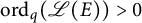


In particular, if $ \operatorname {ord}_q(\mathscr {L}(E)) \le 0 $
and
$ \operatorname {ord}_q(\mathscr {L}(E)) \le 0 $
and $ \overline {\rho _{E, q}} $
is surjective, then compute the Legendre symbols
$ \overline {\rho _{E, q}} $
is surjective, then compute the Legendre symbols
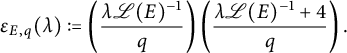
Then for any $ \lambda \in \mathbb {F}_q $
,
$ \lambda \in \mathbb {F}_q $
,
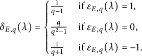 $$ \begin{align*}\delta_{E, q}(\lambda) = \begin{cases} \tfrac{1}{q - 1} & \text{if} \ \epsilon_{E, q}(\lambda) = 1, \\[5pt] \tfrac{q}{q^2 - 1} & \text{if} \ \epsilon_{E, q}(\lambda) = 0, \\[5pt] \tfrac{1}{q + 1} & \text{if} \ \epsilon_{E, q}(\lambda) = -1. \end{cases} \end{align*} $$
Proof By Corollary 3.7, $ \delta _{E, q}(\lambda ) $
is just the natural density of
$ \delta _{E, q}(\lambda ) $
is just the natural density of $ -\mathscr {L}(E)\#E(\mathbb {F}_p) \equiv \lambda \ \mod q $
. If
$ -\mathscr {L}(E)\#E(\mathbb {F}_p) \equiv \lambda \ \mod q $
. If $ \operatorname {ord}_q(\mathscr {L}(E))> 0 $
, then only
$ \operatorname {ord}_q(\mathscr {L}(E))> 0 $
, then only $ \lambda = 0 $
gives a nonzero natural density. Otherwise
$ \lambda = 0 $
gives a nonzero natural density. Otherwise $ \operatorname {ord}_q(\mathscr {L}(E)) \le 0 $
, then this is equivalent to
$ \operatorname {ord}_q(\mathscr {L}(E)) \le 0 $
, then this is equivalent to $ 1 + p - a_p(E) \equiv -\lambda \mathscr {L}(E)^{-1} \ \mod q^m $
, noting that
$ 1 + p - a_p(E) \equiv -\lambda \mathscr {L}(E)^{-1} \ \mod q^m $
, noting that $ \mathscr {L}(E)^{-1} $
is well-defined and nonzero modulo
$ \mathscr {L}(E)^{-1} $
is well-defined and nonzero modulo $ q^m $
by definition. By Chebotarev’s density theorem, this occurs with the proportion of matrices
$ q^m $
by definition. By Chebotarev’s density theorem, this occurs with the proportion of matrices $ M \in G_{E, q} $
with
$ M \in G_{E, q} $
with $ \det (M) = p $
and
$ \det (M) = p $
and $ \operatorname {tr}(M) = a_p(E) $
, so that the second statement follows. If
$ \operatorname {tr}(M) = a_p(E) $
, so that the second statement follows. If $ \overline {\rho _{E, q}} $
is surjective, then Theorem 4.4.1 yields
$ \overline {\rho _{E, q}} $
is surjective, then Theorem 4.4.1 yields $ m = 1 $
, so that
$ m = 1 $
, so that $ \delta _{E, q}(\lambda ) $
is the proportion of matrices
$ \delta _{E, q}(\lambda ) $
is the proportion of matrices $ M \in \operatorname {SL}_2(\mathbb {Z} / q) $
such that
$ M \in \operatorname {SL}_2(\mathbb {Z} / q) $
such that $ \operatorname {tr}(M) \equiv 2 - \lambda \mathscr {L}(E)^{-1} \ \mod q $
. The final statement then follows by
$ \operatorname {tr}(M) \equiv 2 - \lambda \mathscr {L}(E)^{-1} \ \mod q $
. The final statement then follows by $ \#\operatorname {SL}_2(\mathbb {Z} / q) = (q - 1)q(q + 1) $
and by inspecting the possible traces in
$ \#\operatorname {SL}_2(\mathbb {Z} / q) = (q - 1)q(q + 1) $
and by inspecting the possible traces in $ \operatorname {SL}_2(\mathbb {Z} / q) $
as in Section 2, noting that
$ \operatorname {SL}_2(\mathbb {Z} / q) $
as in Section 2, noting that $ \operatorname {tr}(M) = x + x^{-1} $
for some
$ \operatorname {tr}(M) = x + x^{-1} $
for some $ x \in \mathbb {F}_q \setminus \{\pm 1\} $
precisely when
$ x \in \mathbb {F}_q \setminus \{\pm 1\} $
precisely when $ x^2 - 4 $
is a quadratic residue modulo
$ x^2 - 4 $
is a quadratic residue modulo $ q $
.
$ q $
.
Remark 6.2 Without the assumption that $ q \nmid c_0(E) $
, the same argument can be used to compute the residual density of
$ q \nmid c_0(E) $
, the same argument can be used to compute the residual density of $ c_0(E)\mathscr {L}(E, \chi ) $
instead, by adding a factor of
$ c_0(E)\mathscr {L}(E, \chi ) $
instead, by adding a factor of $ c_0(E) $
to every instance of
$ c_0(E) $
to every instance of $ \mathscr {L}(E) $
in the statement and proof of Proposition 6.1. However, Proposition 3.5 predicts that
$ \mathscr {L}(E) $
in the statement and proof of Proposition 6.1. However, Proposition 3.5 predicts that $ \mathscr {L}(E, \chi ) \in \mathbb {Z}[\zeta _q] $
under Stevens’s conjecture, so that both sides of the congruence are divisible by
$ \mathscr {L}(E, \chi ) \in \mathbb {Z}[\zeta _q] $
under Stevens’s conjecture, so that both sides of the congruence are divisible by $ q $
and the statement becomes vacuous.
$ q $
and the statement becomes vacuous.
Remark 6.3 Under the standard arithmetic conjectures, Proposition 5.1 says that $ \mathscr {L}(E, \chi )\zeta \in \mathbb {Z}[\zeta _q] $
, so that
$ \mathscr {L}(E, \chi )\zeta \in \mathbb {Z}[\zeta _q] $
, so that $ \operatorname {Nm}_q^+(\mathscr {L}(E, \chi )\zeta ) $
is an integer. Since the norm is multiplicative and
$ \operatorname {Nm}_q^+(\mathscr {L}(E, \chi )\zeta ) $
is an integer. Since the norm is multiplicative and $ \zeta \equiv 1 \ \mod (1 - \zeta _q) $
, the asymptotic distribution of the residue class of
$ \zeta \equiv 1 \ \mod (1 - \zeta _q) $
, the asymptotic distribution of the residue class of $ \operatorname {Nm}_q^+(\mathscr {L}(E, \chi )\zeta ) $
modulo
$ \operatorname {Nm}_q^+(\mathscr {L}(E, \chi )\zeta ) $
modulo $ q $
essentially boils down to computing
$ q $
essentially boils down to computing $ \delta _{E, q} $
.
$ \delta _{E, q} $
.
Assuming the $ q $
-part of the Birch–Swinnerton-Dyer conjecture, Theorem 4.4.3 says
$ q $
-part of the Birch–Swinnerton-Dyer conjecture, Theorem 4.4.3 says $ \operatorname {ord}_q(\operatorname {BSD}(E)) \ge -1 $
, so that nontrivial values of
$ \operatorname {ord}_q(\operatorname {BSD}(E)) \ge -1 $
, so that nontrivial values of $ \delta _{E, q} $
are only visible when
$ \delta _{E, q} $
are only visible when $ \operatorname {ord}_q(\operatorname {BSD}(E)) \in \{0, -1\} $
. Once this is determined, computing
$ \operatorname {ord}_q(\operatorname {BSD}(E)) \in \{0, -1\} $
. Once this is determined, computing $ \delta _{E, q} $
then reduces to identifying
$ \delta _{E, q} $
then reduces to identifying $ \operatorname {im}(\overline {\rho _{E, q}}) $
or
$ \operatorname {im}(\overline {\rho _{E, q}}) $
or $ \operatorname {im}(\overline {\rho _{E, q^2}}) $
, and then weighing the proportion of matrices with a certain determinant and trace. To illustrate this in action, the next result describes the possible ordered triples
$ \operatorname {im}(\overline {\rho _{E, q^2}}) $
, and then weighing the proportion of matrices with a certain determinant and trace. To illustrate this in action, the next result describes the possible ordered triples $ (\delta _{E, 3}(0), \delta _{E, 3}(1), \delta _{E, 3}(2)) $
of residual densities, which is only made possible thanks to the classification of
$ (\delta _{E, 3}(0), \delta _{E, 3}(1), \delta _{E, 3}(2)) $
of residual densities, which is only made possible thanks to the classification of $ 3 $
-adic Galois images by Rouse–Sutherland–Zureick-Brown [Reference Rouse, Sutherland and Zureick-Brown25, Corollaries 1.3.1 and 12.3.3]. As in the introduction, these ordered triples will also be denoted
$ 3 $
-adic Galois images by Rouse–Sutherland–Zureick-Brown [Reference Rouse, Sutherland and Zureick-Brown25, Corollaries 1.3.1 and 12.3.3]. As in the introduction, these ordered triples will also be denoted $ \delta _{E, 3} $
for ease of notation.
$ \delta _{E, 3} $
for ease of notation.
Theorem 6.4 Let $ E $
be an elliptic curve such that
$ E $
be an elliptic curve such that $ L(E, 1) \ne 0 $
and that
$ L(E, 1) \ne 0 $
and that $ 3 \nmid c_0(E) $
. Assume further that
$ 3 \nmid c_0(E) $
. Assume further that $ \operatorname {ord}_3(\mathscr {L}(E)) = \operatorname {ord}_3(\operatorname {BSD}(E)) $
. Then precisely one of the following holds.
$ \operatorname {ord}_3(\mathscr {L}(E)) = \operatorname {ord}_3(\operatorname {BSD}(E)) $
. Then precisely one of the following holds.
-
(1) If
$ \operatorname {ord}_3(\operatorname {BSD}(E))> 0 $
, then
$ \delta _{E, 3} = (1, 0, 0) $
. -
(2) If
$ \operatorname {ord}_3(\operatorname {BSD}(E)) = 0 $
and
$ 3 \mid \#\operatorname {tor}(E) $
, then
$ \delta _{E, 3} = (1, 0, 0) $
. -
(3) If
$ \operatorname {ord}_3(\operatorname {BSD}(E)) = 0 $
and
$ 3 \nmid \#\operatorname {tor}(E) $
, then
$ \delta _{E, 3} $
is given by the table in Section A.1. -
(4) If
$ \operatorname {ord}_3(\operatorname {BSD}(E)) = -1 $
, then
$ \delta _{E, 3} $
is given by the table in Section A.2.


In particular, $ \delta _{E, 3} $
only depends on
$ \delta _{E, 3} $
only depends on $ \operatorname {BSD}(E) $
and
$ \operatorname {BSD}(E) $
and $ \operatorname {im}(\overline {\rho _{E, 9}}) $
, and can only be one of
$ \operatorname {im}(\overline {\rho _{E, 9}}) $
, and can only be one of
 $$ \begin{align*}(1, 0, 0), \ \left(\tfrac{3}{8}, \tfrac{3}{8}, \tfrac{1}{4}\right), \ \left(\tfrac{3}{8}, \tfrac{1}{4}, \tfrac{3}{8}\right), \ \left(\tfrac{1}{2}, \tfrac{1}{2}, 0\right), \ \left(\tfrac{1}{2}, 0, \tfrac{1}{2}\right), \ \left(\tfrac{1}{8}, \tfrac{3}{4}, \tfrac{1}{8}\right),\end{align*} $$
 $$ \begin{align*}\left(\tfrac{1}{8}, \tfrac{1}{8}, \tfrac{3}{4}\right), \ \left(\tfrac{1}{4}, \tfrac{1}{2}, \tfrac{1}{4}\right), \ \left(\tfrac{1}{4}, \tfrac{1}{4}, \tfrac{1}{2}\right), \ \left(\tfrac{5}{9}, \tfrac{2}{9}, \tfrac{2}{9}\right), \ \left(\tfrac{1}{3}, \tfrac{2}{3}, 0\right), \ \left(\tfrac{1}{3}, 0, \tfrac{2}{3}\right).\end{align*} $$
Proof The fact that there are only four possibilities is immediate from Theorem 4.4. By Proposition 6.1, the first statement follows immediately under the assumption that $ \operatorname {ord}_3(\mathscr {L}(E)) = \operatorname {ord}_3(\operatorname {BSD}(E)) $
, while the second statement follows from
$ \operatorname {ord}_3(\mathscr {L}(E)) = \operatorname {ord}_3(\operatorname {BSD}(E)) $
, while the second statement follows from $ 3 \mid 1 + \det (M) - \operatorname {tr}(M) $
for all matrices
$ 3 \mid 1 + \det (M) - \operatorname {tr}(M) $
for all matrices $ M \in \operatorname {im}(\overline {\rho _{E, 3}}) $
whenever
$ M \in \operatorname {im}(\overline {\rho _{E, 3}}) $
whenever $ 3 \mid \#\operatorname {tor}(E) $
.
$ 3 \mid \#\operatorname {tor}(E) $
.
For the third statement, it suffices to consider $ G_{E, 3} = \operatorname {im}(\overline {\rho _{E, 3}}) \cap \operatorname {SL}_2(\mathbb {Z} / 3) $
, and there are only
$ G_{E, 3} = \operatorname {im}(\overline {\rho _{E, 3}}) \cap \operatorname {SL}_2(\mathbb {Z} / 3) $
, and there are only $ 5 $
possibilities for
$ 5 $
possibilities for $ \operatorname {im}(\overline {\rho _{E, 3}}) $
when
$ \operatorname {im}(\overline {\rho _{E, 3}}) $
when $ \overline {\rho _{E, 3}} $
is not surjective, as tabulated in the table in Section A.1. If
$ \overline {\rho _{E, 3}} $
is not surjective, as tabulated in the table in Section A.1. If $ \overline {\rho _{E, 3}} $
is surjective, then
$ \overline {\rho _{E, 3}} $
is surjective, then $ \delta _{E, 3} $
is already computed in the final statement in Proposition 6.1, while the other
$ \delta _{E, 3} $
is already computed in the final statement in Proposition 6.1, while the other $ 5 $
cases are similar but easier computations. For instance, if
$ 5 $
cases are similar but easier computations. For instance, if $ \operatorname {im}(\overline {\rho _{E, 3}}) $
is 3B.1.2, then
$ \operatorname {im}(\overline {\rho _{E, 3}}) $
is 3B.1.2, then $ G_{E, 3} $
is conjugate to the subgroup of unipotent upper triangular matrices in
$ G_{E, 3} $
is conjugate to the subgroup of unipotent upper triangular matrices in $ \operatorname {SL}_2(\mathbb {Z} / 3) $
. There are
$ \operatorname {SL}_2(\mathbb {Z} / 3) $
. There are $ 6 $
matrices in this subgroup, all of which have trace
$ 6 $
matrices in this subgroup, all of which have trace $ 0 $
, so that
$ 0 $
, so that $ \delta _{E, 3} = (1, 0, 0) $
. Note that when
$ \delta _{E, 3} = (1, 0, 0) $
. Note that when $ \delta _{E, 3}(1) \ne \delta _{E, 3}(2) $
, the nonzero residue of
$ \delta _{E, 3}(1) \ne \delta _{E, 3}(2) $
, the nonzero residue of $ \operatorname {BSD}(E) $
modulo
$ \operatorname {BSD}(E) $
modulo $ 3 $
would swap the values of
$ 3 $
would swap the values of $ \delta _{E, 3}(1) $
and
$ \delta _{E, 3}(1) $
and $ \delta _{E, 3}(2) $
. For instance, if
$ \delta _{E, 3}(2) $
. For instance, if $ \overline {\rho _{E, 3}} $
is surjective, then
$ \overline {\rho _{E, 3}} $
is surjective, then $ G_{E, 3} = \operatorname {SL}_2(\mathbb {Z} / 3) $
, and
$ G_{E, 3} = \operatorname {SL}_2(\mathbb {Z} / 3) $
, and
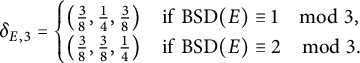 $$ \begin{align*}\delta_{E, 3} = \begin{cases} \left(\tfrac{3}{8}, \tfrac{1}{4}, \tfrac{3}{8}\right) & \text{if} \ \operatorname{BSD}(E) \equiv 1 \quad\mod 3, \\ \left(\tfrac{3}{8}, \tfrac{3}{8}, \tfrac{1}{4}\right) & \text{if} \ \operatorname{BSD}(E) \equiv 2 \quad\mod 3. \end{cases} \end{align*} $$
For the fourth statement, it suffices to consider $ G_{E, 9} $
, and by the classification this is simply the projection onto
$ G_{E, 9} $
, and by the classification this is simply the projection onto $ \operatorname {GL}_2(\mathbb {Z} / 9) $
of
$ \operatorname {GL}_2(\mathbb {Z} / 9) $
of $ 21 $
different possible
$ 21 $
different possible $ \operatorname {im}(\rho _{E, 3}) $
, as tabulated in the table in Section A.2. For instance, if
$ \operatorname {im}(\rho _{E, 3}) $
, as tabulated in the table in Section A.2. For instance, if $ \operatorname {im}(\rho _{E, 3}) $
is 3.8.0.1, then
$ \operatorname {im}(\rho _{E, 3}) $
is 3.8.0.1, then $ G_{E, 9} $
is the preimage of the subgroup of
$ G_{E, 9} $
is the preimage of the subgroup of $ \operatorname {SL}_2(\mathbb {Z} / 3) $
generated by
$ \operatorname {SL}_2(\mathbb {Z} / 3) $
generated by $ (\begin {smallmatrix} 1 & 2 \\ 0 & 1 \end {smallmatrix}) $
and
$ (\begin {smallmatrix} 1 & 2 \\ 0 & 1 \end {smallmatrix}) $
and $ (\begin {smallmatrix} 1 & 2 \\ 0 & 2 \end {smallmatrix}) $
under the canonical projection
$ (\begin {smallmatrix} 1 & 2 \\ 0 & 2 \end {smallmatrix}) $
under the canonical projection $ \operatorname {GL}_2(\mathbb {Z} / 9) \twoheadrightarrow \operatorname {GL}_2(\mathbb {Z} / 3) $
. This preimage in
$ \operatorname {GL}_2(\mathbb {Z} / 9) \twoheadrightarrow \operatorname {GL}_2(\mathbb {Z} / 3) $
. This preimage in $ \operatorname {GL}_2(\mathbb {Z} / 9) $
consists of
$ \operatorname {GL}_2(\mathbb {Z} / 9) $
consists of $ 243 $
matrices, of which
$ 243 $
matrices, of which $ 135 $
have trace
$ 135 $
have trace $ 0 $
and
$ 0 $
and $ 54 $
have trace
$ 54 $
have trace $ 1 $
and
$ 1 $
and $ 2 $
each, so that
$ 2 $
each, so that
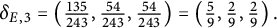 $$ \begin{align*}\delta_{E, 3} = \left(\tfrac{135}{243}, \tfrac{54}{243}, \tfrac{54}{243}\right) = \left(\tfrac{5}{9}, \tfrac{2}{9}, \tfrac{2}{9}\right).\end{align*} $$
The other $ 20 $
cases are similar but easier computations, noting again that the nonzero residue of
$ 20 $
cases are similar but easier computations, noting again that the nonzero residue of $ 3\operatorname {BSD}(E) $
modulo
$ 3\operatorname {BSD}(E) $
modulo $ 3 $
would swap the values of
$ 3 $
would swap the values of $ \delta _{E, 3}(1) $
and
$ \delta _{E, 3}(1) $
and $ \delta _{E, 3}(2) $
when
$ \delta _{E, 3}(2) $
when $ \delta _{E, 3}(1) \ne \delta _{E, 3}(2) $
. For instance, if
$ \delta _{E, 3}(1) \ne \delta _{E, 3}(2) $
. For instance, if $ \operatorname {im}(\rho _{E, 3}) $
is 27.648.18.1, then
$ \operatorname {im}(\rho _{E, 3}) $
is 27.648.18.1, then
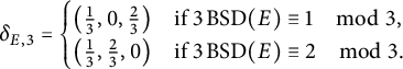 $$ \begin{align*}\delta_{E, 3} = \begin{cases} \left(\tfrac{1}{3}, 0, \tfrac{2}{3}\right) & \text{if} \ 3\operatorname{BSD}(E) \equiv 1 \quad\mod 3, \\ \left(\tfrac{1}{3}, \tfrac{2}{3}, 0\right) & \text{if} \ 3\operatorname{BSD}(E) \equiv 2 \quad\mod 3. \end{cases} \end{align*} $$
Finally, the final statement follows immediately from the first four.
Remark 6.5 The first case happens when $ 3 \nmid \#\operatorname {tor}(E) $
but
$ 3 \nmid \#\operatorname {tor}(E) $
but ![]() , such as for the elliptic curve 50b4 where
, such as for the elliptic curve 50b4 where $ \operatorname {BSD}(E) = 3 $
, and the second case happens when
$ \operatorname {BSD}(E) = 3 $
, and the second case happens when ![]() , such as for the elliptic curve 84a1 where
, such as for the elliptic curve 84a1 where $ \operatorname {BSD}(E) = \tfrac {1}{2} $
.
$ \operatorname {BSD}(E) = \tfrac {1}{2} $
.
Remark 6.6 If $ \operatorname {im}(\overline {\rho _{E, 3}}) $
is 3Cs.1.1, then a much easier argument to prove that
$ \operatorname {im}(\overline {\rho _{E, 3}}) $
is 3Cs.1.1, then a much easier argument to prove that $ \delta _{E, 3} = (1, 0, 0) $
is to observe that
$ \delta _{E, 3} = (1, 0, 0) $
is to observe that $ G_{E, 3} $
is trivial, so that
$ G_{E, 3} $
is trivial, so that $ E(\mathbb {F}_p) $
acquires full
$ E(\mathbb {F}_p) $
acquires full $ 3 $
-torsion for any
$ 3 $
-torsion for any $ p \equiv 1 \ \mod 3 $
, and thus
$ p \equiv 1 \ \mod 3 $
, and thus $ \mathscr {L}(E, \chi ) \equiv -\operatorname {BSD}(E)\#E(\mathbb {F}_p) \equiv 0 \ \mod 3 $
always.
$ \mathscr {L}(E, \chi ) \equiv -\operatorname {BSD}(E)\#E(\mathbb {F}_p) \equiv 0 \ \mod 3 $
always.


7 Twisted L-values of Kisilevsky–Nam
The computation of residual densities was originally motivated by patterns in the statistical data by Kisilevsky–Nam [Reference Kisilevsky and Nam18, Section 7], where they numerically computed millions of modified twisted L-values by fixing the elliptic curve and varying the character. However, they considered an alternative normalization, given by
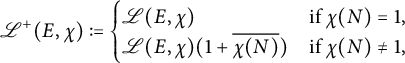
in contrast to the normalization factor $ \zeta $
given in Proposition 5.1. Under the implicit assumption that
$ \zeta $
given in Proposition 5.1. Under the implicit assumption that $ \mathscr {L}(E, \chi ) \in \mathbb {Z}[\zeta _q] $
, they showed that
$ \mathscr {L}(E, \chi ) \in \mathbb {Z}[\zeta _q] $
, they showed that $ \mathscr {L}^+(E, \chi ) \in \mathbb {Z}[\zeta _q]^+ $
[Reference Kisilevsky and Nam18, Proposition 2.1], so that
$ \mathscr {L}^+(E, \chi ) \in \mathbb {Z}[\zeta _q]^+ $
[Reference Kisilevsky and Nam18, Proposition 2.1], so that $ \operatorname {Nm}_q^+(\mathscr {L}^+(E, \chi )) $
is an integer. Fixing six elliptic curves
$ \operatorname {Nm}_q^+(\mathscr {L}^+(E, \chi )) $
is an integer. Fixing six elliptic curves $ E $
and five small integers
$ E $
and five small integers $ q $
, they varied the character
$ q $
, they varied the character $ \chi $
of order
$ \chi $
of order $ q $
over millions of conductors
$ q $
over millions of conductors $ p $
with an arbitrary choice of
$ p $
with an arbitrary choice of $ \chi $
for each
$ \chi $
for each $ p $
, empirically determined the greatest common divisor
$ p $
, empirically determined the greatest common divisor $ \gcd _{E, q} $
of all the integers
$ \gcd _{E, q} $
of all the integers $ \operatorname {Nm}_q^+(\mathscr {L}^+(E, \chi )) $
, and considered the integer
$ \operatorname {Nm}_q^+(\mathscr {L}^+(E, \chi )) $
, and considered the integer
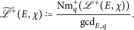
Remark 7.1 When $ q $
is odd and
$ q $
is odd and $ L(E, 1) \ne 0 $
, this definition of
$ L(E, 1) \ne 0 $
, this definition of $ \widetilde {\mathscr {L}}^+(E, \chi ) $
coincides with the modified twisted L-value denoted
$ \widetilde {\mathscr {L}}^+(E, \chi ) $
coincides with the modified twisted L-value denoted $ A_\chi $
by Kisilevsky–Nam, since
$ A_\chi $
by Kisilevsky–Nam, since $ \chi (N) = -1 $
never occurs and the global root number is always
$ \chi (N) = -1 $
never occurs and the global root number is always $ 1 $
[Reference Kisilevsky and Nam18, Section 2.2]. Their definition of
$ 1 $
[Reference Kisilevsky and Nam18, Section 2.2]. Their definition of $ \mathscr {L}(E, \chi ) $
has an extra factor of
$ \mathscr {L}(E, \chi ) $
has an extra factor of $ 2 $
, but this is cancelled out after division by
$ 2 $
, but this is cancelled out after division by $ \gcd _{E, q} $
.
$ \gcd _{E, q} $
.
Remark 7.2 In the interpretation of Proposition 5.1, the integer $ \gcd _{E, q} $
is predicted to arise from contributions by the common divisors of
$ \gcd _{E, q} $
is predicted to arise from contributions by the common divisors of $ \operatorname {BSD}(E / K) / \operatorname {BSD}(E) $
, ranging over various number fields
$ \operatorname {BSD}(E / K) / \operatorname {BSD}(E) $
, ranging over various number fields $ K $
of degree
$ K $
of degree $ q $
over
$ q $
over $ \mathbb {Q} $
coming from characters of order
$ \mathbb {Q} $
coming from characters of order $ q $
.
$ q $
.
As their normalization differs from that in Proposition 5.1 [Reference Kisilevsky and Nam18, Remark 1], the resulting residual densities are skewed. More precisely, define the set $ X_{E, q}^{< n} $
as before, and analogously define the skewed residual densities
$ X_{E, q}^{< n} $
as before, and analogously define the skewed residual densities $ \widetilde {\delta }_{E, q} $
of
$ \widetilde {\delta }_{E, q} $
of $ \widetilde {\mathscr {L}}^+(E, \chi ) $
to be the natural densities of
$ \widetilde {\mathscr {L}}^+(E, \chi ) $
to be the natural densities of $ \widetilde {\mathscr {L}}^+(E, \chi ) $
modulo
$ \widetilde {\mathscr {L}}^+(E, \chi ) $
modulo $ q $
. In other words, this is the value
$ q $
. In other words, this is the value
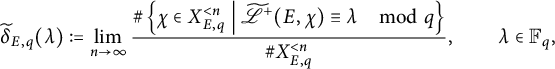
if such a limit exists. In the simplest case where $ q = 3 \nmid \gcd _{E, 3} $
,
$ q = 3 \nmid \gcd _{E, 3} $
,
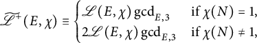 $$ \begin{align*} \widetilde{{\mathscr{L}}}^+(E, \chi) \equiv\begin{cases}{\mathscr{L}}(E, \chi)\gcd_{E, 3} & \text{if} \ \chi(N) = 1, \\2{\mathscr{L}}(E, \chi)\gcd_{E, 3} & \text{if} \ \chi(N) \ne 1,\end{cases} \end{align*} $$
since there is no norm. This becomes amenable to a computation similar to that of Proposition 6.1 provided that the condition $ \chi (N) = 1 $
can be controlled. For many elliptic curves, including half of those considered by Kisilevsky–Nam,
$ \chi (N) = 1 $
can be controlled. For many elliptic curves, including half of those considered by Kisilevsky–Nam, $ \chi (N) $
depends completely on
$ \chi (N) $
depends completely on $ \#E(\mathbb {F}_p) $
due to a shared action of Frobenius in
$ \#E(\mathbb {F}_p) $
due to a shared action of Frobenius in $ \operatorname {GL}_2(\mathbb {Z} / 3) $
.
$ \operatorname {GL}_2(\mathbb {Z} / 3) $
.
Lemma 7.3 Let $ E $
be an elliptic curve of conductor
$ E $
be an elliptic curve of conductor $ N $
with no rational
$ N $
with no rational $ 3 $
-isogeny such that the splitting field
$ 3 $
-isogeny such that the splitting field $ F $
of
$ F $
of $ X^3 - N $
lies in the splitting field
$ X^3 - N $
lies in the splitting field $ K $
of the
$ K $
of the $ 3 $
-division polynomial
$ 3 $
-division polynomial $ \psi _{E, 3} $
. Let
$ \psi _{E, 3} $
. Let $ \chi $
be a cubic character of odd prime conductor
$ \chi $
be a cubic character of odd prime conductor $ p \nmid N $
. Then
$ p \nmid N $
. Then $ \operatorname {im}(\overline {\rho _{E, 3}}) = \operatorname {GL}_2(\mathbb {Z} / 3) $
and
$ \operatorname {im}(\overline {\rho _{E, 3}}) = \operatorname {GL}_2(\mathbb {Z} / 3) $
and $ \operatorname {Gal}(K / \mathbb {Q}) \cong \operatorname {PGL}_2(\mathbb {Z} / 3) $
. Furthermore, if
$ \operatorname {Gal}(K / \mathbb {Q}) \cong \operatorname {PGL}_2(\mathbb {Z} / 3) $
. Furthermore, if $ p $
does not split completely in
$ p $
does not split completely in $ K $
, then
$ K $
, then $ \#E(\mathbb {F}_p) \equiv 2 \ \mod 3 $
if and only if
$ \#E(\mathbb {F}_p) \equiv 2 \ \mod 3 $
if and only if $ \chi (N) = 1 $
. Otherwise,
$ \chi (N) = 1 $
. Otherwise, $ \#E(\mathbb {F}_p) \not \equiv 2 \ \mod 3 $
and
$ \#E(\mathbb {F}_p) \not \equiv 2 \ \mod 3 $
and $ \chi (N) = 1 $
.
$ \chi (N) = 1 $
.
Proof Let $ L $
be the extension of
$ L $
be the extension of $ K $
where all points in
$ K $
where all points in $ E[3] $
are defined. By the assumption that
$ E[3] $
are defined. By the assumption that $ E $
has no rational
$ E $
has no rational $ 3 $
-isogeny and the classification of
$ 3 $
-isogeny and the classification of $ \operatorname {im}(\overline {\rho _{E, 3}}) $
, if
$ \operatorname {im}(\overline {\rho _{E, 3}}) $
, if $ \overline {\rho _{E, 3}} $
were not surjective, then
$ \overline {\rho _{E, 3}} $
were not surjective, then $ \operatorname {Gal}(L / \mathbb {Q}) $
is either 3Nn or 3Ns. Neither of this could occur, since by the assumption that
$ \operatorname {Gal}(L / \mathbb {Q}) $
is either 3Nn or 3Ns. Neither of this could occur, since by the assumption that $ F \subseteq K $
, there are subfield inclusions
$ F \subseteq K $
, there are subfield inclusions
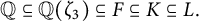 $$ \begin{align*}\mathbb{Q} \subseteq \mathbb{Q}(\zeta_3) \subseteq F \subseteq K \subseteq L.\end{align*} $$
In particular, $ \operatorname {Gal}(L / \mathbb {Q}) $
surjects onto
$ \operatorname {Gal}(L / \mathbb {Q}) $
surjects onto $ \operatorname {Gal}(F / \mathbb {Q}) \cong \mathcal {S}_3 $
, which forces
$ \operatorname {Gal}(F / \mathbb {Q}) \cong \mathcal {S}_3 $
, which forces $ \operatorname {Gal}(L / \mathbb {Q}) \cong \operatorname {GL}_2(\mathbb {Z} / 3) $
. On the other hand,
$ \operatorname {Gal}(L / \mathbb {Q}) \cong \operatorname {GL}_2(\mathbb {Z} / 3) $
. On the other hand, $ \operatorname {Gal}(K / \mathbb {Q}) $
permutes the roots of the degree
$ \operatorname {Gal}(K / \mathbb {Q}) $
permutes the roots of the degree $ 4 $
polynomial
$ 4 $
polynomial $ \psi _{E, 3} $
, which forces it to be
$ \psi _{E, 3} $
, which forces it to be $ \operatorname {PGL}_2(\mathbb {Z} / 3) \cong \mathcal {S}_4 $
. Its subgroup
$ \operatorname {PGL}_2(\mathbb {Z} / 3) \cong \mathcal {S}_4 $
. Its subgroup $ \operatorname {Gal}(K / \mathbb {Q}(\zeta _3)) \cong \mathcal {A}_4 $
surjects onto
$ \operatorname {Gal}(K / \mathbb {Q}(\zeta _3)) \cong \mathcal {A}_4 $
surjects onto $ \operatorname {Gal}(F / \mathbb {Q}(\zeta _3)) \cong \mathbb {Z} / 3 $
, with kernel the unique subgroup
$ \operatorname {Gal}(F / \mathbb {Q}(\zeta _3)) \cong \mathbb {Z} / 3 $
, with kernel the unique subgroup $ \operatorname {Gal}(K / F) \cong (\mathbb {Z} / 2)^2 $
of index
$ \operatorname {Gal}(K / F) \cong (\mathbb {Z} / 2)^2 $
of index $ 4 $
consisting precisely of all elements of
$ 4 $
consisting precisely of all elements of $ \mathcal {A}_4 $
of order
$ \mathcal {A}_4 $
of order $ 1 $
or
$ 1 $
or $ 2 $
.
$ 2 $
.
Now $ \operatorname {Fr}_p \in \operatorname {Gal}(K / \mathbb {Q}) $
acts on the residue field of a prime
$ \operatorname {Fr}_p \in \operatorname {Gal}(K / \mathbb {Q}) $
acts on the residue field of a prime $ \pi $
of
$ \pi $
of $ F $
above
$ F $
above $ p $
by
$ p $
by
 $$ \begin{align*}\operatorname{Fr}_p(\zeta_3) \equiv \zeta_3^p \quad\mod \pi, \qquad \operatorname{Fr}_p(\sqrt[3]{N}) \equiv \sqrt[3]{N}^p \quad\mod \pi.\end{align*} $$
Clearly $ \operatorname {Fr}_p $
fixes
$ \operatorname {Fr}_p $
fixes $ \zeta _3 $
, so that
$ \zeta _3 $
, so that $ \operatorname {Fr}_p \in \operatorname {Gal}(K / \mathbb {Q}(\zeta _3)) $
. If
$ \operatorname {Fr}_p \in \operatorname {Gal}(K / \mathbb {Q}(\zeta _3)) $
. If $ p $
does not split completely in
$ p $
does not split completely in $ K $
, the condition
$ K $
, the condition $ \operatorname {Fr}_p \in \operatorname {Gal}(K / F) $
turns out to be equivalent to
$ \operatorname {Fr}_p \in \operatorname {Gal}(K / F) $
turns out to be equivalent to $ \#E(\mathbb {F}_p) \equiv 2 \ \mod 3 $
and to
$ \#E(\mathbb {F}_p) \equiv 2 \ \mod 3 $
and to $ \chi (N) = 1 $
. To see this, on one hand, this means that
$ \chi (N) = 1 $
. To see this, on one hand, this means that $ \operatorname {Fr}_p $
fixes
$ \operatorname {Fr}_p $
fixes $ \sqrt [3]{N} $
, or equivalently that
$ \sqrt [3]{N} $
, or equivalently that $ \sqrt [3]{N}^{p - 1} \equiv 1 \ \mod p $
, which is precisely the condition that
$ \sqrt [3]{N}^{p - 1} \equiv 1 \ \mod p $
, which is precisely the condition that $ \chi (N) = 1 $
. On the other hand, this also means that
$ \chi (N) = 1 $
. On the other hand, this also means that $ \operatorname {Fr}_p^2 = 1 $
in
$ \operatorname {Fr}_p^2 = 1 $
in $ \operatorname {Gal}(K / \mathbb {Q}(\zeta _3)) $
, which is equivalent to
$ \operatorname {Gal}(K / \mathbb {Q}(\zeta _3)) $
, which is equivalent to $ \operatorname {Fr}_p $
having order exactly
$ \operatorname {Fr}_p $
having order exactly $ 2 $
in
$ 2 $
in $ \operatorname {Gal}(K / \mathbb {Q}(\zeta _3)) $
. By the Cayley–Hamilton theorem, these are precisely the trace
$ \operatorname {Gal}(K / \mathbb {Q}(\zeta _3)) $
. By the Cayley–Hamilton theorem, these are precisely the trace $ 0 $
matrices in
$ 0 $
matrices in $ \operatorname {PGL}_2(\mathbb {Z} / 3) $
, or equivalently the trace
$ \operatorname {PGL}_2(\mathbb {Z} / 3) $
, or equivalently the trace $ 0 $
matrices in
$ 0 $
matrices in $ \operatorname {GL}_2(\mathbb {Z} / 3) $
, which proves the equivalence with
$ \operatorname {GL}_2(\mathbb {Z} / 3) $
, which proves the equivalence with $ a_p(E) = 0 $
. Finally, if
$ a_p(E) = 0 $
. Finally, if $ p $
splits completely in
$ p $
splits completely in $ K $
, then
$ K $
, then $ \operatorname {Fr}_p = 1 $
in
$ \operatorname {Fr}_p = 1 $
in $ \operatorname {Gal}(K / \mathbb {Q}(\zeta _3)) $
, and hence
$ \operatorname {Gal}(K / \mathbb {Q}(\zeta _3)) $
, and hence $ \chi (N) = 1 $
, but these never have trace
$ \chi (N) = 1 $
, but these never have trace $ 0 $
in
$ 0 $
in $ \operatorname {PGL}_2(\mathbb {Z} / 3) $
or in
$ \operatorname {PGL}_2(\mathbb {Z} / 3) $
or in $ \operatorname {GL}_2(\mathbb {Z} / 3) $
, so that
$ \operatorname {GL}_2(\mathbb {Z} / 3) $
, so that $ \#E(\mathbb {F}_p) \not \equiv 2 \ \mod 3 $
.
$ \#E(\mathbb {F}_p) \not \equiv 2 \ \mod 3 $
.
Remark 7.4 The first assumption is necessary, evident in the elliptic curve 50b1 with $ F \subseteq K $
but
$ F \subseteq K $
but $ \operatorname {im}(\overline {\rho _{E, 3}}) $
is 3B, where
$ \operatorname {im}(\overline {\rho _{E, 3}}) $
is 3B, where $ 7 $
does not split completely in
$ 7 $
does not split completely in $ K $
but
$ K $
but $ \#E(\mathbb {F}_7) = 10 \equiv 1 \ \mod 3 $
and
$ \#E(\mathbb {F}_7) = 10 \equiv 1 \ \mod 3 $
and $ \chi (50) = \overline {\chi (50)} = 1 $
. The second assumption is also necessary, evident in the elliptic curve 21a1 with no rational
$ \chi (50) = \overline {\chi (50)} = 1 $
. The second assumption is also necessary, evident in the elliptic curve 21a1 with no rational $ 3 $
-isogeny but
$ 3 $
-isogeny but $ F \not \subseteq K $
, where
$ F \not \subseteq K $
, where $ 13 $
does not split completely in
$ 13 $
does not split completely in $ K $
but
$ K $
but $ \#E(\mathbb {F}_{13}) = 16 \equiv 1 \ \mod 3 $
and
$ \#E(\mathbb {F}_{13}) = 16 \equiv 1 \ \mod 3 $
and $ \chi (21) = \overline {\chi (21)} = 1 $
. For the final statement, checking that
$ \chi (21) = \overline {\chi (21)} = 1 $
. For the final statement, checking that $ p $
splits completely in
$ p $
splits completely in $ F $
but not in
$ F $
but not in $ K $
is not sufficient to conclude, such as for the elliptic curve 11a1, where
$ K $
is not sufficient to conclude, such as for the elliptic curve 11a1, where $ \#E(\mathbb {F}_{19}) = 20 \equiv 2 \ \mod 3 $
and
$ \#E(\mathbb {F}_{19}) = 20 \equiv 2 \ \mod 3 $
and $ \chi (11) = \overline {\chi (11)} = 1 $
. If
$ \chi (11) = \overline {\chi (11)} = 1 $
. If $ p $
does split completely in
$ p $
does split completely in $ K $
, then both
$ K $
, then both $ \#E(\mathbb {F}_p) \equiv 0 \ \mod 3 $
and
$ \#E(\mathbb {F}_p) \equiv 0 \ \mod 3 $
and $ \#E(\mathbb {F}_p) \equiv 1 \ \mod 3 $
are possible, such as for the elliptic curve 11a1, where
$ \#E(\mathbb {F}_p) \equiv 1 \ \mod 3 $
are possible, such as for the elliptic curve 11a1, where $ \#E(\mathbb {F}_{337}) = 360 \equiv 0 \ \mod 3 $
and
$ \#E(\mathbb {F}_{337}) = 360 \equiv 0 \ \mod 3 $
and $ \#E(\mathbb {F}_{193}) = 190 \equiv 1 \ \mod 3 $
.
$ \#E(\mathbb {F}_{193}) = 190 \equiv 1 \ \mod 3 $
.
Remark 7.5 The argument in the proof of Lemma 7.3 only works for cubic characters, as $ \operatorname {PGL}_2(\mathbb {Z} / q) $
is almost simple for
$ \operatorname {PGL}_2(\mathbb {Z} / q) $
is almost simple for $ q> 3 $
and admits few nontrivial surjections.
$ q> 3 $
and admits few nontrivial surjections.
Remark 7.6 Elliptic curves with minimal discriminant $ \Delta = \pm N^n $
for some
$ \Delta = \pm N^n $
for some $ n \in \mathbb {N} $
such that
$ n \in \mathbb {N} $
such that $ 3 \nmid n $
satisfy the assumptions of Lemma 7.3, since
$ 3 \nmid n $
satisfy the assumptions of Lemma 7.3, since $ \sqrt [3]{N} $
can then be expressed in terms of
$ \sqrt [3]{N} $
can then be expressed in terms of $ \sqrt [3]{\Delta } $
[Reference Serre26, Section 5.3b]. This condition is in turn satisfied when
$ \sqrt [3]{\Delta } $
[Reference Serre26, Section 5.3b]. This condition is in turn satisfied when $ N $
is prime, such as for the elliptic curves given by
$ N $
is prime, such as for the elliptic curves given by $ y^2 = x^3 + ux^2 - 16x $
and
$ y^2 = x^3 + ux^2 - 16x $
and $ y^2 = x^3 - 2ux^2 + Nx $
studied by Neumann [Reference Neumann24, Theorem 5.1] and Setzer [Reference Setzer27, Theorem 2] when
$ y^2 = x^3 - 2ux^2 + Nx $
studied by Neumann [Reference Neumann24, Theorem 5.1] and Setzer [Reference Setzer27, Theorem 2] when $ N = u^2 + 64 $
for some integer
$ N = u^2 + 64 $
for some integer $ u $
, which occurs infinitely often assuming Bunyakovsky’s conjecture.
$ u $
, which occurs infinitely often assuming Bunyakovsky’s conjecture.
For these elliptic curves, the residual density of $ \widetilde {\mathscr {L}}^+(E, \chi ) $
is now easy to compute.
$ \widetilde {\mathscr {L}}^+(E, \chi ) $
is now easy to compute.
Proposition 7.7 Let $ E $
be an elliptic curve of conductor
$ E $
be an elliptic curve of conductor $ N $
with no rational
$ N $
with no rational $ 3 $
-isogeny such that
$ 3 $
-isogeny such that $ 3 \nmid c_0(E)\gcd _{E, 3} $
and that the splitting field
$ 3 \nmid c_0(E)\gcd _{E, 3} $
and that the splitting field $ F $
of
$ F $
of $ X^3 - N $
lies in the splitting field
$ X^3 - N $
lies in the splitting field $ K $
of the
$ K $
of the $ 3 $
-division polynomial
$ 3 $
-division polynomial $ \psi _{E, 3} $
. Let
$ \psi _{E, 3} $
. Let $ \chi $
be a cubic character of odd prime conductor
$ \chi $
be a cubic character of odd prime conductor $ p \nmid N $
. Then
$ p \nmid N $
. Then
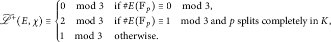 $$ \begin{align*}\widetilde{\mathscr{L}}^+(E, \chi) \equiv \begin{cases} 0 \quad\mod 3 & \text{if} \ \#E(\mathbb{F}_p) \equiv 0 \quad\mod 3, \\ 2 \quad\mod 3 & \text{if} \ \#E(\mathbb{F}_p) \equiv 1 \quad\mod 3 \ \text{and} \ p \ \text{splits completely in} \ K, \\ 1 \quad\mod 3 & \text{otherwise}. \end{cases} \end{align*} $$
In particular,
 $$ \begin{align*}\widetilde{\delta}_{E, 3}(0) = \tfrac{9}{24}, \qquad \widetilde{\delta}_{E, 3}(1) = \tfrac{15}{24}, \qquad \widetilde{\delta}_{E, 3}(2) = \tfrac{1}{24}.\end{align*} $$
Proof By Corollary 3.7 and the assumption that $ 3 \nmid c_0(E)\gcd _{E, 3} $
,
$ 3 \nmid c_0(E)\gcd _{E, 3} $
,
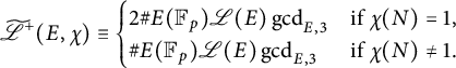 $$ \begin{align*}\widetilde{\mathscr{L}}^+(E, \chi) \equiv \begin{cases} 2\#E(\mathbb{F}_p)\mathscr{L}(E)\gcd_{E, 3} & \text{if} \ \chi(N) = 1, \\ \#E(\mathbb{F}_p)\mathscr{L}(E)\gcd_{E, 3} & \text{if} \ \chi(N) \ne 1. \end{cases} \end{align*} $$
Clearly $ \widetilde {\mathscr {L}}^+(E, \chi ) \equiv 0 \ \mod 3 $
when
$ \widetilde {\mathscr {L}}^+(E, \chi ) \equiv 0 \ \mod 3 $
when $ \#E(\mathbb {F}_p) \equiv 0 \ \mod 3 $
. By Lemma 7.3,
$ \#E(\mathbb {F}_p) \equiv 0 \ \mod 3 $
. By Lemma 7.3, $ \chi (N) = 1 $
occurs either when
$ \chi (N) = 1 $
occurs either when $ \#E(\mathbb {F}_p) \equiv 1 \ \mod 3 $
but
$ \#E(\mathbb {F}_p) \equiv 1 \ \mod 3 $
but $ p $
splits completely in
$ p $
splits completely in $ K $
, or when
$ K $
, or when $ \#E(\mathbb {F}_p) \equiv 2 \ \mod 3 $
but
$ \#E(\mathbb {F}_p) \equiv 2 \ \mod 3 $
but $ p $
does not split completely in
$ p $
does not split completely in $ K $
, the only remaining case being when
$ K $
, the only remaining case being when $ \#E(\mathbb {F}_p) \equiv 1 \ \mod 3 $
and
$ \#E(\mathbb {F}_p) \equiv 1 \ \mod 3 $
and $ \chi (N) \ne 1 $
. The first statement then follows by substituting the residues of
$ \chi (N) \ne 1 $
. The first statement then follows by substituting the residues of $ \#E(\mathbb {F}_p) $
modulo
$ \#E(\mathbb {F}_p) $
modulo $ 3 $
, and noting that
$ 3 $
, and noting that $ \gcd _{E, 3} $
cancels out the factors in
$ \gcd _{E, 3} $
cancels out the factors in $ \mathscr {L}(E) $
by definition. Now the description of the groups in Lemma 7.3 implies that
$ \mathscr {L}(E) $
by definition. Now the description of the groups in Lemma 7.3 implies that $ \#E(\mathbb {F}_p) \equiv \lambda \ \mod 3 $
occurs with the proportion of matrices
$ \#E(\mathbb {F}_p) \equiv \lambda \ \mod 3 $
occurs with the proportion of matrices $ M \in \operatorname {SL}_2(\mathbb {Z} / 3) $
with
$ M \in \operatorname {SL}_2(\mathbb {Z} / 3) $
with $ \operatorname {tr}(M) = 2 - \lambda $
, by Chebotarev’s density theorem. If
$ \operatorname {tr}(M) = 2 - \lambda $
, by Chebotarev’s density theorem. If $ p $
splits completely in
$ p $
splits completely in $ K $
, then
$ K $
, then $ \operatorname {Fr}_p = 1 $
in
$ \operatorname {Fr}_p = 1 $
in $ \operatorname {PGL}_2(\mathbb {Z} / 3) $
, so that
$ \operatorname {PGL}_2(\mathbb {Z} / 3) $
, so that $ \operatorname {Fr}_p = \pm 1 $
in
$ \operatorname {Fr}_p = \pm 1 $
in $ \operatorname {GL}_2(\mathbb {Z} / 3) $
and in
$ \operatorname {GL}_2(\mathbb {Z} / 3) $
and in $ \operatorname {SL}_2(\mathbb {Z} / 3) $
, but the condition
$ \operatorname {SL}_2(\mathbb {Z} / 3) $
, but the condition $ \#E(\mathbb {F}_p) \equiv 1 \ \mod 3 $
forces
$ \#E(\mathbb {F}_p) \equiv 1 \ \mod 3 $
forces $ \operatorname {Fr}_p = -1 $
, which has trace
$ \operatorname {Fr}_p = -1 $
, which has trace $ 1 $
. The final statement then follows by counting matrices in
$ 1 $
. The final statement then follows by counting matrices in $ \operatorname {SL}_2(\mathbb {Z} / 3) $
with given trace.
$ \operatorname {SL}_2(\mathbb {Z} / 3) $
with given trace.
Proposition 7.7 completely explains the numerical data by Kisilevsky–Nam for the elliptic curve 11a1 where $ \gcd _{E, 3} = 5 $
and the elliptic curves 15a1 and 17a1 where
$ \gcd _{E, 3} = 5 $
and the elliptic curves 15a1 and 17a1 where $ \gcd _{E, 3} = 4 $
, all of which satisfy the assumptions of Proposition 7.7. Unfortunately, the same argument cannot explain the density patterns when
$ \gcd _{E, 3} = 4 $
, all of which satisfy the assumptions of Proposition 7.7. Unfortunately, the same argument cannot explain the density patterns when $ 3 \mid \gcd _{E, 3} $
, such as for the remaining three elliptic curves 14a1, 19a1, and 37b1 considered by Kisilevsky–Nam, since Corollary 3.7 is a priori not valid modulo
$ 3 \mid \gcd _{E, 3} $
, such as for the remaining three elliptic curves 14a1, 19a1, and 37b1 considered by Kisilevsky–Nam, since Corollary 3.7 is a priori not valid modulo $ 9 $
, as noted in Remark 3.9.
$ 9 $
, as noted in Remark 3.9.
A Tables of Galois images
This section tabulates the mod- $ 3 $
and
$ 3 $
and $ 3 $
-adic Galois images of elliptic curves
$ 3 $
-adic Galois images of elliptic curves $ E $
with restricted
$ E $
with restricted $ 3 $
-torsion up to conjugacy, crucially used in Proposition 4.2 and Theorem 6.4. In both tables, the examples of elliptic curves are chosen so that it has the smallest conductor possible satisfying
$ 3 $
-torsion up to conjugacy, crucially used in Proposition 4.2 and Theorem 6.4. In both tables, the examples of elliptic curves are chosen so that it has the smallest conductor possible satisfying $ L(E, 1) \ne 0 $
and
$ L(E, 1) \ne 0 $
and $ 3 \mid c_0(E) $
, but in general there are many elliptic curves with each prescribed mod-
$ 3 \mid c_0(E) $
, but in general there are many elliptic curves with each prescribed mod- $ 3 $
or
$ 3 $
or $ 3 $
-adic Galois image.
$ 3 $
-adic Galois image.
A.1 Mod-3 Galois images of elliptic curves without 3-torsion
The possible mod- $ 3 $
Galois images are well-known [Reference Zywina35, Theorem 1.2 and Propositions 1.14 and 1.16], and those of elliptic curves without
$ 3 $
Galois images are well-known [Reference Zywina35, Theorem 1.2 and Propositions 1.14 and 1.16], and those of elliptic curves without $ 3 $
-torsion are tabulated as follows. The subgroup labels and generators are taken from Sutherland [Reference Sutherland31, Section 6.4], and are viewed as elements of
$ 3 $
-torsion are tabulated as follows. The subgroup labels and generators are taken from Sutherland [Reference Sutherland31, Section 6.4], and are viewed as elements of $ \operatorname {GL}_2(\mathbb {Z} / 3) $
. The column
$ \operatorname {GL}_2(\mathbb {Z} / 3) $
. The column $ G_{E, 3} $
lists the elements of
$ G_{E, 3} $
lists the elements of $ G_{E, 3} = \operatorname {im}(\overline {\rho _{E, 3}}) \cap \operatorname {SL}_2(\mathbb {Z} / 3) $
as defined in Proposition 6.1, so that the residual densities can be read off directly in the column
$ G_{E, 3} = \operatorname {im}(\overline {\rho _{E, 3}}) \cap \operatorname {SL}_2(\mathbb {Z} / 3) $
as defined in Proposition 6.1, so that the residual densities can be read off directly in the column $ \delta _{E, 3} $
as ordered triples
$ \delta _{E, 3} $
as ordered triples $ (\delta _{E, 3}(0), \delta _{E, 3}(-b), \delta _{E, 3}(b)) $
, where
$ (\delta _{E, 3}(0), \delta _{E, 3}(-b), \delta _{E, 3}(b)) $
, where $ b \in \mathbb {F}_3 $
is the residue of
$ b \in \mathbb {F}_3 $
is the residue of $ \operatorname {BSD}(E) $
modulo
$ \operatorname {BSD}(E) $
modulo $ 3 $
, which is used in Theorem 6.4. The final column
$ 3 $
, which is used in Theorem 6.4. The final column $ E $
gives examples of elliptic curves
$ E $
gives examples of elliptic curves $ E $
with the given mod-
$ E $
with the given mod- $ 3 $
Galois image, with
$ 3 $
Galois image, with $ b = 1 $
in the first row and
$ b = 1 $
in the first row and $ b = 2 $
in the second row.
$ b = 2 $
in the second row.
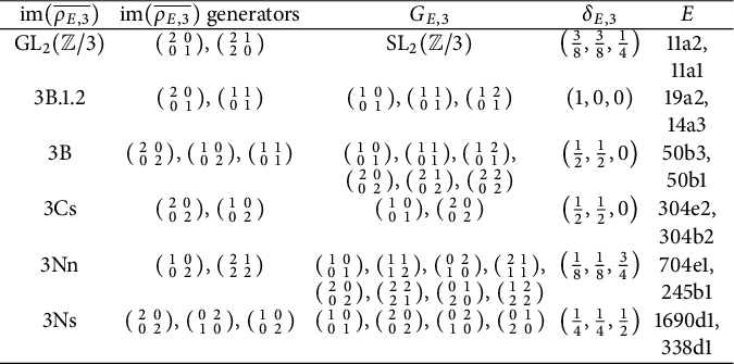
The remaining two mod- $ 3 $
Galois images 3B.1.1 and 3Cs.1.1 have
$ 3 $
Galois images 3B.1.1 and 3Cs.1.1 have $ 3 $
-torsion, so the residual densities require finer information from their mod-
$ 3 $
-torsion, so the residual densities require finer information from their mod- $ 9 $
Galois images.
$ 9 $
Galois images.
A.2 3-adic Galois images of elliptic curves with 3-torsion
The possible $ 3 $
-adic Galois images have been classified [Reference Rouse, Sutherland and Zureick-Brown25, Corollaries 1.3.1 and 12.3.3], and those of elliptic curves with
$ 3 $
-adic Galois images have been classified [Reference Rouse, Sutherland and Zureick-Brown25, Corollaries 1.3.1 and 12.3.3], and those of elliptic curves with $ 3 $
-torsion are tabulated as follows. The subgroup labels and generators are taken from Rouse–Sutherland–Zureick-Brown [Reference Rouse, Sutherland and Zureick-Brown25, Software Repository], and are viewed as elements of
$ 3 $
-torsion are tabulated as follows. The subgroup labels and generators are taken from Rouse–Sutherland–Zureick-Brown [Reference Rouse, Sutherland and Zureick-Brown25, Software Repository], and are viewed as elements of $ \operatorname {GL}_2(\mathbb {Z} / 3^m) $
if their corresponding
$ \operatorname {GL}_2(\mathbb {Z} / 3^m) $
if their corresponding $ 3 $
-adic Galois images are of the form
$ 3 $
-adic Galois images are of the form $ 3^m.i.g.n $
. The column
$ 3^m.i.g.n $
. The column $ M_{E, 3} $
gives matrices
$ M_{E, 3} $
gives matrices $ M \in \operatorname {im}(\overline {\rho _{E, 9}}) $
such that
$ M \in \operatorname {im}(\overline {\rho _{E, 9}}) $
such that $ 1 + \det (M) - \operatorname {tr}(M) = 3 $
, which is used in Proposition 4.2. The column
$ 1 + \det (M) - \operatorname {tr}(M) = 3 $
, which is used in Proposition 4.2. The column $ \#G_{E, 9} $
lists the cardinalities of
$ \#G_{E, 9} $
lists the cardinalities of $ G_{E, 9} $
as defined in Proposition 6.1 for reference, but the residual densities are calculated separately in the column
$ G_{E, 9} $
as defined in Proposition 6.1 for reference, but the residual densities are calculated separately in the column $ \delta _{E, 3} $
as ordered triples
$ \delta _{E, 3} $
as ordered triples $ (\delta _{E, 3}(0), \delta _{E, 3}(-b), \delta _{E, 3}(b)) $
, where
$ (\delta _{E, 3}(0), \delta _{E, 3}(-b), \delta _{E, 3}(b)) $
, where $ b \in \mathbb {F}_3 $
is the residue of
$ b \in \mathbb {F}_3 $
is the residue of $ 3\operatorname {BSD}(E) $
modulo
$ 3\operatorname {BSD}(E) $
modulo $ 3 $
, which is used in Theorem 6.4. The final column
$ 3 $
, which is used in Theorem 6.4. The final column $ E $
gives examples of elliptic curves
$ E $
gives examples of elliptic curves $ E $
with the given
$ E $
with the given $ 3 $
-adic Galois image, assuming they exist and are listed in the LMFDB, with
$ 3 $
-adic Galois image, assuming they exist and are listed in the LMFDB, with $ b = 1 $
in the first row and
$ b = 1 $
in the first row and $ b = 2 $
in the second row if it exists.
$ b = 2 $
in the second row if it exists.
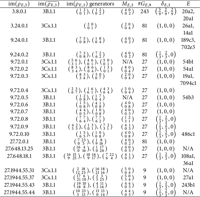
Remark A.1 Many of the $ 3 $
-adic Galois images seemingly do not represent any elliptic curves with
$ 3 $
-adic Galois images seemingly do not represent any elliptic curves with $ b \ne 0 $
, in the sense that a search through the LMFDB yields no examples satisfying
$ b \ne 0 $
, in the sense that a search through the LMFDB yields no examples satisfying $ L(E, 1) \ne 0 $
and
$ L(E, 1) \ne 0 $
and $ 3 \mid c_0(E) $
, but current results a priori do not rule out their existence. To rule out examples for a specific
$ 3 \mid c_0(E) $
, but current results a priori do not rule out their existence. To rule out examples for a specific $ 3 $
-adic Galois image, one could consider the explicit family of Weierstrass equations parameterized by the associated modular curve, and then investigate the divisibility of local Tamagawa numbers as in Lemma 4.1, but this will not be explored here. Note that this is the case for the last six
$ 3 $
-adic Galois image, one could consider the explicit family of Weierstrass equations parameterized by the associated modular curve, and then investigate the divisibility of local Tamagawa numbers as in Lemma 4.1, but this will not be explored here. Note that this is the case for the last six $ 3 $
-adic Galois images arising from elliptic curves with complex multiplication, where their associated modular curves have effectively computable finite sets of rational points.
$ 3 $
-adic Galois images arising from elliptic curves with complex multiplication, where their associated modular curves have effectively computable finite sets of rational points.
Acknowledgements
I would like to thank Vladimir Dokchitser for suggesting the problem and guidance throughout the project. I would also like to thank Peiran Wu and Jacob Fjeld Grevstad for assistance on some group theory arguments, as well as Harry Spencer and the four anonymous reviewers for feedback on prior drafts.


 Open access