To save content items to your account,
please confirm that you agree to abide by our usage policies.
If this is the first time you use this feature, you will be asked to authorise Cambridge Core to connect with your account.
Find out more about saving content to .
To save content items to your Kindle, first ensure no-reply@cambridge.org
is added to your Approved Personal Document E-mail List under your Personal Document Settings
on the Manage Your Content and Devices page of your Amazon account. Then enter the ‘name’ part
of your Kindle email address below.
Find out more about saving to your Kindle.
Note you can select to save to either the @free.kindle.com or @kindle.com variations.
‘@free.kindle.com’ emails are free but can only be saved to your device when it is connected to wi-fi.
‘@kindle.com’ emails can be delivered even when you are not connected to wi-fi, but note that service fees apply.
A solid material subjected to mechanical and thermal loading will change shape and develop internal stresses. What is the best way to describe this? In principle, the behavior of a material (neglecting relativistic effects) is dictated by that of its atoms, which are governed by quantum mechanics. Therefore, if we could solve Schrödinger's equation (see Chapter 4) for 1023 atoms and evolve the dynamics of the electrons and nuclei over “macroscopic times” (i.e. seconds, hours and days) we would be able to predict material behavior. Of course when we say “material,” we are already referring to a very complex system as demonstrated in the previous chapter. In order to predict the response of the material we would first have to construct its structure in the computer, which would require us to use Schrödinger's equation to simulate the process by which it was manufactured. Conceptually, it is useful to think of materials in this way, but we can quickly see the futility of the approach; state-of-the-art quantum calculations involve mere hundreds of atoms over a time of nanoseconds.
At the other extreme to quantum mechanics lie continuum mechanics and thermodynamics. These disciplines completely ignore the discreteness of the world, treating it in terms of “macroscopic observables,” time and space averages over the underlying swirling masses of atoms. This leads to a theory couched in terms of continuously varying fields. Using clear thinking inspired by experiments it is possible to construct a remarkably coherent and predictive framework for material behavior.
Chapters 4 and 5 were essentially about ways to estimate the potential energy of configurations of atoms. In this chapter, we discuss how we can use these potential energy landscapes to understand phenomena in materials science. Generally, this is done by studying key features in the potential energy landscape (local minima and the transition paths between them) using the methods of molecular statics (MS). After discussing some of the details of implementing MS algorithms, we will turn to several example applications in crystalline materials in Section 6.5.
The potential energy landscape
Using quantum mechanics, density functional theory (DFT) or tight-binding (TB) we are able to compute the energy of the electrons given the fixed positions of the atomic nuclei, and add this to the Coulomb interactions between the nuclei to get the total potential energy. In developing empirical methods, we approximated this electronic energy as a potential energy function dependent on only the interatomic distances. In either case, we are able to compute the potential energy, V = V(r), of any arbitrary configuration of N atoms, with positions r = (r1, …, rN). We refer to the set of all possible coordinates {rα} as the configuration space of our system. Much of this configuration space is likely to be unphysical or at least impractical; we can create virtual atomic configurations on a computer that are very unlikely ever to occur in nature.
The governing equations of continuum mechanics and thermodynamics were derived in Chapter 2 based on the fundamental laws of physics and the assumption of local thermodynamic equilibrium. These equations, summarized at the start of Section 2.5, provide relationships between a number of different continuum fields: density ρ(x), velocity v(x), Cauchy stress σ(x), heat flux q(x), temperature T(x), entropy s(x), and the internal energy density u(x). In the continuum worldview these entities are primitive quantities that emerge as part of the framework of the theory. When solving a continuum problem it is not necessary to know “what” they are as long as experiments can be devised to measure the constitutive relations that connect them. This view of continuum mechanics was strongly held by its early developers as evidenced by the quote in footnote 17 on page 43.
The objective of this chapter is to go beyond the phenomenological approach of classical continuum mechanics and thermodynamics by establishing a direct connection with the underlying atomistic system. Our motivation for doing so is not to prove that the continuum theories are correct (there is ample proof for this by their success), but rather to provide a mechanism for computing continuum measures in molecular simulations. This is important in order to be able to extract constitutive relations from “computer experiments” and to help rationalize the results of such simulations in the language of continuum mechanics.
When we say that a problem in science is “multiscale,” we broadly mean that it involves phenomena at disparate length and/or time scales spanning several orders of magnitude. More importantly, these phenomena all play key roles in the problem, so that we cannot correctly model the interesting behavior without explicitly accounting for these different scales. In Chapter 1, we looked at a wide range of length and time scales relevant to materials modeling, motivating the case that materials science is filled with multiscale problems. Indeed, the message we have tried to carry throughout this book is that there is a need to model materials at many scales, and to make connections between them. However, when we speak of multiscale modeling, we tend to be referring to something more specific, meaning that the problem is tackled with a conscious effort to span multiple scales simultaneously.
In many cases, multiscale methods involve just two scales, a “coarse scale” and “fine scale”, each of which plays a role in the problem. Depending on the perspective, multiscale models offer different advantages. For the fine-scale modeler, a multiscale approach allows one to study much larger systems (or longer times) than could be studied using the finescale alone. On the other hand, the coarse-scale expert views the multiscale model as a way to establish the constitutive laws of the problem from first principles, or at least from a more fundamental scientific basis than could be realized from the coarse-scale alone.
In the preface to his book on the subject, Peierls says of the quantum theory of solids [Pei64]
[It] has sometimes the reputation of being rather less respectable than other branches of modern theoretical physics. The reason for this view is that the dynamics of many-body systems, with which it is concerned, cannot be handled without the use of simplifications, or without approximations which often omit essential features of the problem.
This book, in essence, is all about ways to further approximate the quantum theory of solids; it is about ways to build approximate models that describe the collective behavior of quantum mechanical atoms in materials. Whether it is the development of density functional theory (DFT), empirical classical interatomic potentials, continuum constitutive laws or multiscale methods, one can only conclude that, by Peierls' measure, modeling materials is a science that is a great deal less respectable than even the quantum theory of solids itself. However, Peierls goes on to say that
Nevertheless, the [quantum] theory [of solids] contains a good deal of work of intrinsic interest in which one can either develop a solution convincingly from first principles, or at least give a clear picture of the features which have been omitted and therefore discuss qualitatively the changes which they are likely to cause.
It is our view that these redeeming qualities are equally applicable to the modern science of modeling materials.
In the previous chapter, we saw the enormous complexity that governs the bonding of solids. Electronic interactions and structure in the presence of the positively charged ionic cores can only be fully understood using the machinery of Schrödinger's equation and quantum mechanics. But the simplest of bonding problems, that of two hydrogen atoms, is already too complex to solve exactly. Density functional theory (DFT), whereby Schrödinger's equation is recast in a form amenable to numerical solution, provides us with a powerful tool for accurately solving complex bonding problems, but at the expense of significant computational effort. Tight-binding (TB) reduces the burden by parameterizingmany of the integrals in DFT into simple analytic forms, but still requires expensive matrix inversion. To have any hope of modeling the complex deformation problems of interest to us (see, for example, Chapter 6), we must rely on much more approximate approaches for describing the atomic interactions using fitted functional forms.
As we saw in Section 4.5, the TB formulation provides a bridge between DFT and empirical potentials. However, given the boldness of some of the approximations that take us from full quantum mechanics to TB, one might question why empirical models should work at all. It is true that we must view all empirical results suspiciously. In some cases they can be quite accurate, while in others we may only be able to use them as idealized models that capture the general trends or basic mechanisms of the real systems.
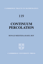
Many phenomena in physics, chemistry, and biology can be modelled by spatial random processes. One such process is continuum percolation, which is used when the phenomenon being modelled is made up of individual events that overlap, for example, the way individual raindrops eventually make the ground evenly wet. This is a systematic rigorous account of continuum percolation. Two models, the Boolean model and the random connection model, are treated in detail, and related continuum models are discussed. All important techniques and methods are explained and applied to obtain results on the existence of phase transitions, equality and continuity of critical densities, compressions, rarefaction, and other aspects of continuum models. This self-contained treatment, assuming only familiarity with measure theory and basic probability theory, will appeal to students and researchers in probability and stochastic geometry.
This book explains key concepts and methods in the field of ordinary differential equations. It assumes only minimal mathematical prerequisites but, at the same time, introduces the reader to the way ordinary differential equations are used in current mathematical research and in scientific modelling. It is designed as a practical guide for students and aspiring researchers in any mathematical science - in which I include, besides mathematics itself, physics, engineering, computer science, probability theory, statistics and the quantitative side of chemistry, biology, economics and finance.
The subject of differential equations is vast and this book only deals with initial value problems for ordinary differential equations. Such problems are fundamental in modern science since they arise when one tries to predict the future from knowledge about the present. Applications of differential equations in the physical and biological sciences occupy a prominent place both in the main text and in the exercises. Numerical methods for solving differential equations are not studied in any detail, but the use of mathematical software for solving differential equations and plotting functions is encouraged and sometimes required.
How to use this book
The book should be useful for students at a range of levels and with a variety of scientific backgrounds, provided they have studied differential and integral calculus (including partial derivatives), elements of real analysis (such as ∈δ-definitions of continuity and differentiability), complex numbers and linear algebra. It could serve as a textbook for a first course on ordinary differential equations for undergraduates on a mathematics, science, engineering or economics degree who have studied the prerequisites listed above.
Differential equations of second order occur frequently in applied mathematics, particularly in applications coming from physics and engineering. The main reason for this is that most fundamental equations of physics, like Newton's second law of motion (2. 7), are second order differential equations. It is not clear why Nature, at a fundamental level, should obey second order differential equations, but that is what centuries of research have taught us.
Since second order ODEs and even systems of second order ODEs are special cases of systems of first order ODEs, one might think that the study of second order ODEs is a simple application of the theory studied in Chapter 2. This is true as far as general existence and uniqueness questions are concerned, but there are a number of elementary techniques especially designed for solving second order ODEs which are more efficient than the general machinery developed for systems. In this chapter we briefly review these techniques and then look in detail at the application of second order ODEs in the study of oscillations. If there is one topic in physics that every mathematician should know about then this is it. Much understanding of a surprisingly wide range of physical phenomena can be gained from studying the equation governing a mass attached to a spring and acted on by an external force. Conversely, one can develop valuable intuition about second order differential equations from a thorough understanding of the physics of the oscillating spring.
This chapter contains five projects which develop the ideas and techniques introduced in this book. The first four projects are all based on recent research publications. Their purpose is to illustrate the variety of ways in which ODEs arise in contemporary research - ranging from engineering to differential geometry - and to provide an authentic opportunity for the reader to apply the techniques of the previous chapters. If possible, the projects could be tackled by a small group of students working as a team. The fifth project has a different flavour. Its purpose is to guide the reader through the proof of the Picard-Lindelöf Theorem. At the beginning of each project, I indicate the parts of the book which contain relevant background material.
Ants on polygons
(Background: Chapters 1 and 2, Exercise 2. 6)
Do you remember the problem of four ants chasing each other at constant speed, studied in Exercise 2. 6? We now look at two variations of this problem. In the first, we consider n ants, where n = 2, 3, 4, 5 …, starting off on a regular n-gon. Here, a 2-gon is simply a line, a regular 3-gon an equilateral triangle, a 4-gon a square and so on. In the second, more diffcult, variation we consider 4 ants starting their pursuit on a rectangle with side lengths in the ratio 1:2. This innocent-sounding generalisation turns out to be remarkably subtle and rich, and is the subject of recent research reported in Chapman, Lottes and Trefethen [4].
This book has one purpose: to help you understand vectors and tensors so that you can use them to solve problems. If you're like most students, you first encountered vectors when you took a course dealing with mechanics in high school or college. At that level, you almost certainly learned that vectors are mathematical representations of quantities that have both magnitude and direction, such as velocity and force. You may also have learned how to add vectors graphically and by using their components in the x-, y- and z-directions.
That's a fine place to start, but it turns out that such treatments only scratch the surface of the power of vectors. You can harness that power and make it work for you if you're willing to delve a bit deeper – to see vectors not just as objects with magnitude and direction, but rather as objects that behave in very predictable ways when viewed from different reference frames. That's because vectors are a subset of a larger class of objects called “tensors,” which most students encounter much later in their academic careers, and which have been called “the facts of the Universe.” It is no exaggeration to say that our understanding of the fundamental structure of the universe was changed forever when Albert Einstein succeeded in expressing his theory of gravity in terms of tensors.
If you were tracking the main ideas of Chapter 1, you should realize that vectors are representations of physical quantities – they're mathematical tools that help you visualize and describe a physical situation. In this chapter, you can read about a variety of ways to use those tools to solve problems. You've already seen how to add vectors and how to multiply vectors by a scalar (and why such operations are useful); this chapter contains many other “vector operations” through which you can combine and manipulate vectors. Some of these operations are simple and some are more complex, but each will prove useful in solving problems in physics and engineering. The first section of this chapter explains the simplest form of vector multiplication: the scalar product.
Scalar product
Why is it worth your time to understand the form of vector multiplication called the scalar or “dot” product? For one thing, forming the dot product between two vectors is very useful when you're trying to find the projection of one vector onto another. And why might you want to do that? Well, you may be interested in knowing how much work is done by a force acting on an object. The first instinct of many students is to think of work as “force times distance” (which is a reasonable starting point).