


1. Introduction
Time-dependent systems, including periodic, quasi-periodic and chaotic dynamical systems, can exhibit complex behaviours. These behaviours are often more intricate compared to those of autonomous systems. By studying time-dependent flows, engineers and scientists can better predict and control the fluid dynamics in oscillatory flow systems, leading to improved designs and more efficient processes across multiple disciplines, including rheology characterisation, wave energy conversion, modelling of pulsatile blood flows and medical diagnostics. One of the fundamental time-dependent systems in fluid mechanics is the Stokes layer, a thin fluid layer near a solid boundary subject to a periodic motion, named after Sir George Gabriel Stokes. Analytical solutions exist for this flow, and stability analyses of these solutions have been conducted extensively in the past due to their theoretical significance. However, the physical mechanism underpinning the flow transition in Stokes layers remains poorly understood (Davis Reference Davis1976). This study aims to address the longstanding discrepancy between theoretical predictions and experimental observations in transitional Stokes layers by investigating their intracyclic instability.
As a time-periodic flow system, the linear dynamics of the Stokes layer has been initially studied using the Floquet theory by von Kerczek & Davis (Reference von Kerczek and Davis1974) and Hall (Reference Hall1978). Leveraging more powerful computational resources, Blennerhassett & Bassom (Reference Blennerhassett and Bassom2002, Reference Blennerhassett and Bassom2006) were the first to identify an unstable Floquet mode in semi-infinite Stokes layers, determining the critical Reynolds number to be $Re_c\approx 708$
, which is defined based on the Stokes layer thickness. However, experimental studies on the transitional Stokes layers report a broad range of transition Reynolds numbers, from 140 to 300 (Hino et al. 1976, 1983; Jensen, Sumer & Fredsøe Reference Jensen, Sumer and Fredsøe1989; Akhavan et al. Reference Akhavan, Kamm and Shapiro1991a
), significantly lower than the theoretical prediction. This signals a typical subcritical transition scenario.
$Re_c\approx 708$
, which is defined based on the Stokes layer thickness. However, experimental studies on the transitional Stokes layers report a broad range of transition Reynolds numbers, from 140 to 300 (Hino et al. 1976, 1983; Jensen, Sumer & Fredsøe Reference Jensen, Sumer and Fredsøe1989; Akhavan et al. Reference Akhavan, Kamm and Shapiro1991a
), significantly lower than the theoretical prediction. This signals a typical subcritical transition scenario.
While Floquet theory has provided insights into the long-term behaviour of disturbances in time-periodic systems, this approach falls short in capturing the intracyclic instability of the Stokes layer observed experimentally with significant modulation in each oscillation cycle. This has led to the study of instability using instantaneous or momentary stability theory (Cowley Reference Cowley1987; Luo & Wu Reference Luo and Wu2010; Blondeaux & Vittori Reference Blondeaux and Vittori2021), which assesses the local stability by treating the base flow profile as frozen at each moment in time and assuming that the disturbance is of high frequency. The theory typically predicts disturbance decay at the start of the deceleration phase of the wall motion, which conflicts with experimental observations. On the other hand, using the non-normal stability theory, Biau (Reference Biau2016) found large transient energy growth due to the two-dimensional (2-D) Orr mechanism in subcritical semi-infinite Stokes layers. Akhavan et al. (Reference Akhavan, Kamm and Shapiro1991b ) have already observed the transient growth in their experiments, even though they connected their observations to the quasi-steady theory. The non-normal property of the Stokes layers is also evidenced in the exceptionally large flow response investigated by Blennerhassett & Bassom (Reference Blennerhassett and Bassom2002) and Thomas et al. (Reference Thomas, Bassom, Blennerhassett and Davies2010), and the influence of high-frequency noise on the flow explored by Thomas et al. (Reference Thomas, Blennerhassett, Bassom and Davies2015).
Additional factors have been taken into account to further examine the transitional process in the Stokes layer. For example, (weakly) nonlinear stability theories were developed by Monkewitz & Bunster (Reference Monkewitz and Bunster1985) and Wu (Reference Wu1992) to study the nonlinear interaction of the salient modes in the flow. Besides, the role of wall roughness in the transition has been elucidated by Blondeaux & Vittori (Reference Blondeaux and Vittori1994), Vittori & Verzicco (Reference Vittori and Verzicco1998) and Luo & Wu (Reference Luo and Wu2010). However, compelling evidence for a meaningful comparison with experimental results is still lacking. As a result, it remains unclear which theory is most relevant to the flow dynamics in Stokes layers from a practical standpoint. A significant research gap remains in our understanding of how the Stokes layer becomes unstable and transitions to turbulence.
To further clarify the flow instability and transition mechanism in the Stokes layer, this study revisits the linear dynamics of the periodic flow, aiming to determine whether the theory aligns with experimental results. Our focus is on the transient intracyclic instability, analysed through the finite-time Lyapunov exponent (FTLE) framework. Unlike the instantaneous or momentary stability theory, the FTLE analysis inherently incorporates the flow’s evolutionary history, without requiring a frozen base-flow profile. It also connects the transient growth and the numerical abscissa at short times and the Floquet exponent at long times, reconciling and complementing the existing theories. The obtained results in general align with prior experimental and numerical observations.
In the following, we will first formulate the linear equations and then introduce the numerical method to study these equations in § 2. Section 3 will show the results. We first illustrate the finite Stokes layer with $h=5$
(where
$h=5$
(where $h$
is the non-dimensionalised channel half-height, to be defined), corresponding to the case with the maximum transient growth. Then the
$h$
is the non-dimensionalised channel half-height, to be defined), corresponding to the case with the maximum transient growth. Then the $h=10$
case will be analysed and compared to the experimental data. Stokes layers with small
$h=10$
case will be analysed and compared to the experimental data. Stokes layers with small $h$
will be also studied. This is followed by an investigation of the effect of the oscillation frequency, the most practical parameter to vary in experiments, on transient growth. Additionally, nonlinear simulations will be presented to examine both the transient evolution and the saturated dynamics of the Stokes layer. Finally, we conclude the paper with some discussions that underscore the favourable comparison to experimental observations, establishing the non-normal mechanism as the key ingradient for the intracyclic instability in the Stokes layer, and outlining future directions for flow control and nonlinear analysis.
$h$
will be also studied. This is followed by an investigation of the effect of the oscillation frequency, the most practical parameter to vary in experiments, on transient growth. Additionally, nonlinear simulations will be presented to examine both the transient evolution and the saturated dynamics of the Stokes layer. Finally, we conclude the paper with some discussions that underscore the favourable comparison to experimental observations, establishing the non-normal mechanism as the key ingradient for the intracyclic instability in the Stokes layer, and outlining future directions for flow control and nonlinear analysis.
2. Problem formulation and numerical methods
2.1. Formulation
We consider a finite Stokes layer in a channel, subject to a harmonic motion of the two oscillating walls in their own planes. The walls move at the same velocity $U_0\cos \omega \hat t$
, where
$U_0\cos \omega \hat t$
, where $U_0$
is the maximum oscillating velocity, and
$U_0$
is the maximum oscillating velocity, and $\omega$
denotes the oscillating frequency. The hat indicates dimensional variables. The two walls are separated by
$\omega$
denotes the oscillating frequency. The hat indicates dimensional variables. The two walls are separated by $2d$
, with the Cartesian coordinates located at the channel centre. For sufficiently distanced walls, this flow mimics the dynamics of the semi-infinite Stokes layer. The streamwise, wall-normal and transverse directions are denoted by
$2d$
, with the Cartesian coordinates located at the channel centre. For sufficiently distanced walls, this flow mimics the dynamics of the semi-infinite Stokes layer. The streamwise, wall-normal and transverse directions are denoted by $(\hat x,\hat y,\hat z)$
, respectively, corresponding to the velocity components
$(\hat x,\hat y,\hat z)$
, respectively, corresponding to the velocity components $\hat u,\hat v,\hat w$
in the three directions. The streamwise and transverse wavenumbers are represented by
$\hat u,\hat v,\hat w$
in the three directions. The streamwise and transverse wavenumbers are represented by $\alpha$
and
$\alpha$
and $\gamma$
, respectively.
$\gamma$
, respectively.
Following Blennerhassett & Bassom (Reference Blennerhassett and Bassom2002, Reference Blennerhassett and Bassom2006), we non-dimensionalise the flow system using the Stokes layer thickness $\sqrt {2\nu /\omega }$
, the maximum wall-oscillating velocity
$\sqrt {2\nu /\omega }$
, the maximum wall-oscillating velocity $U_0$
, the time scale
$U_0$
, the time scale $1/\omega$
, and the pressure scale
$1/\omega$
, and the pressure scale $\rho U_0^2$
, where
$\rho U_0^2$
, where $\nu$
is the kinematic viscosity coefficient, and
$\nu$
is the kinematic viscosity coefficient, and $\rho$
is the density. The non-dimensional incompressible Navier–Stokes equations read
$\rho$
is the density. The non-dimensional incompressible Navier–Stokes equations read
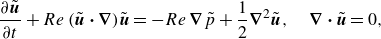 \begin{align} \frac {\partial \tilde {\boldsymbol{u} }}{\partial t} + Re\, (\tilde {\boldsymbol{u}}\boldsymbol{\cdot} \boldsymbol{\nabla} )\tilde {\boldsymbol{u}} = -Re\,\boldsymbol{\nabla} \tilde {p} + \frac {1}{2}\boldsymbol{\nabla} ^2 \tilde {\boldsymbol{u}}, \quad \boldsymbol{\nabla} \boldsymbol{\cdot} \tilde {\boldsymbol{u}}=0, \end{align}
where the Reynolds number is defined as
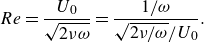 \begin{align} Re=\frac {U_0}{\sqrt {2\nu \omega }} =\frac {1/\omega }{\sqrt {2\nu /\omega }/U_0}. \end{align}
The second equation implies that $Re$
can be thought of as the ratio between the time scale for wall oscillation and the time scale for the ‘penetration’ effect of the wall oscillation. No-slip boundary conditions for the velocity components are imposed on the channel walls. Driven by the non-dimensionalised periodic wall motion
$Re$
can be thought of as the ratio between the time scale for wall oscillation and the time scale for the ‘penetration’ effect of the wall oscillation. No-slip boundary conditions for the velocity components are imposed on the channel walls. Driven by the non-dimensionalised periodic wall motion $\cos t$
, the equations admit an analytical solution of a time-periodic flow
$\cos t$
, the equations admit an analytical solution of a time-periodic flow $\boldsymbol{U}_b$
in the
$\boldsymbol{U}_b$
in the $x$
direction, i.e.
$x$
direction, i.e.
 \begin{align} { {\boldsymbol{U}_b}=(U_b(y,t),0,0) = (U_1(y)\,{\rm e}^{{\rm i}t} + U_1^*(y)\,{\rm e}^{-{\rm i}t}, 0 ,0 ),\quad \text{with} \quad U_1(y) = \frac { \cosh {\sqrt {2{\rm i}}\,y} }{ 2\cosh \sqrt {2{\rm i}}\,h } }, \end{align}
where $h = d/\sqrt {2\nu /\omega }$
denotes the non-dimensional channel half-height,
$h = d/\sqrt {2\nu /\omega }$
denotes the non-dimensional channel half-height, ${\rm i}$
is the imaginary unit, and the superscript
${\rm i}$
is the imaginary unit, and the superscript $^*$
marks the complex conjugate.
$^*$
marks the complex conjugate.
The linear analysis is formulated based on the decomposition of the flow variables into a sum of a base flow plus a fluctuation component, i.e. $\tilde {\boldsymbol{u}}({\boldsymbol{x}},t)={\boldsymbol{U}_b}({\boldsymbol{x}}, t) + {\boldsymbol{u}}({\boldsymbol{x}},t),\ \tilde {p}({\boldsymbol{x}},t)=p({\boldsymbol{x}},t)$
, where there is no base pressure gradient. By substituting these equations into (2.1), expanding all the terms, subtracting the base-flow terms and neglecting the nonlinear terms, we obtain
$\tilde {\boldsymbol{u}}({\boldsymbol{x}},t)={\boldsymbol{U}_b}({\boldsymbol{x}}, t) + {\boldsymbol{u}}({\boldsymbol{x}},t),\ \tilde {p}({\boldsymbol{x}},t)=p({\boldsymbol{x}},t)$
, where there is no base pressure gradient. By substituting these equations into (2.1), expanding all the terms, subtracting the base-flow terms and neglecting the nonlinear terms, we obtain
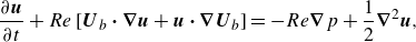 \begin{align} \frac {\partial {\boldsymbol{u}}}{\partial t} + Re\,[ {\boldsymbol{U}_b} \boldsymbol{\cdot} \boldsymbol{\nabla} {\boldsymbol{u}} + {\boldsymbol{u}} \boldsymbol{\cdot} \boldsymbol{\nabla} {\boldsymbol{U}_b} ] & = -Re \boldsymbol{\nabla} p + \frac {1}{2}\boldsymbol{\nabla} ^2 {\boldsymbol{u}}, \end{align}
 \begin{align} \boldsymbol{\nabla} \boldsymbol{\cdot} {\boldsymbol{u}} & = 0. \end{align}
The initial value problem (2.4) can be recast as ${\partial \boldsymbol{u}}/{\partial t}=\boldsymbol{L}(t)\,\boldsymbol{u}$
. In our calculation, the pressure term in the momentum equation was eliminated using the continuity condition, leading to the
${\partial \boldsymbol{u}}/{\partial t}=\boldsymbol{L}(t)\,\boldsymbol{u}$
. In our calculation, the pressure term in the momentum equation was eliminated using the continuity condition, leading to the $v{-}\eta$
formulation based on the vertical velocity
$v{-}\eta$
formulation based on the vertical velocity $v$
and the vertical vorticity
$v$
and the vertical vorticity $\eta = ({\partial u}/{\partial z}) - ({\partial w}/{\partial x})$
. The
$\eta = ({\partial u}/{\partial z}) - ({\partial w}/{\partial x})$
. The $v{-}\eta$
formulation reads
$v{-}\eta$
formulation reads
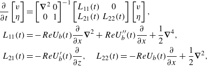 \begin{align} \frac {\partial }{\partial t} \begin{bmatrix} v \\ \eta \end{bmatrix} &= \begin{bmatrix} \boldsymbol{\nabla} ^2 & 0 \\ 0 & 1 \end{bmatrix} ^{-1} \begin{bmatrix} L_{11}(t) & 0 \\ L_{21}(t) & L_{22}(t) \end{bmatrix} \begin{bmatrix} v \\ \eta \end{bmatrix}, \nonumber\\ L_{11}(t)&=-Re U_b(t) \frac {\partial }{\partial x} \boldsymbol{\nabla} ^2+ Re U^{\prime\prime}_b(t)\frac {\partial }{\partial x} + \frac {1}{2}\boldsymbol{\nabla} ^4, \nonumber \\ L_{21}(t)&=- Re U'_b(t)\frac {\partial }{\partial z}, \quad L_{22}(t)=-Re U_b(t) \frac {\partial }{\partial x} + \frac {1}{2}\boldsymbol{\nabla} ^2, \end{align}
where prime $'$
denotes the
$'$
denotes the $y$
derivative. The boundary conditions of the perturbed variables are
$y$
derivative. The boundary conditions of the perturbed variables are $v(\pm h)=v'(\pm h)=\eta (\pm h)=0$
.
$v(\pm h)=v'(\pm h)=\eta (\pm h)=0$
.
To numerically discretise these equations, the classic spectral collocation method (Weideman & Reddy Reference Weideman and Reddy2000) is used for the spatial discretisation, with grid resolution $N_y=69$
(excluding the boundary grid points) in the wall-normal direction. The homogeneous boundary conditions of the variables are implemented by removing the first/last rows and first/last columns of the corresponding matrices in the collocation method. The clamped boundary conditions of
$N_y=69$
(excluding the boundary grid points) in the wall-normal direction. The homogeneous boundary conditions of the variables are implemented by removing the first/last rows and first/last columns of the corresponding matrices in the collocation method. The clamped boundary conditions of $v$
are implemented using the code scripts provided by Weideman & Reddy (Reference Weideman and Reddy2000). The fourth-order backward Euler method is used for time integration, with
$v$
are implemented using the code scripts provided by Weideman & Reddy (Reference Weideman and Reddy2000). The fourth-order backward Euler method is used for time integration, with ${\rm d}t=10^{-5}$
in solving the linear equations.
${\rm d}t=10^{-5}$
in solving the linear equations.
2.2. The FTLE analysis
The FTLE analysis (Lekien, Shadden & Marsden Reference Lekien, Shadden and Marsden2007; Shadden Reference Shadden2012; Haller Reference Haller2015) is traditionally applied to nonlinear flow systems to probe how initially close trajectories are separated with time. The maximum FTLE $\Lambda$
is defined as
$\Lambda$
is defined as
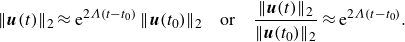 \begin{align} \| \boldsymbol{u}(t)\|_2 \approx {\rm e}^{2\Lambda (t-t_0)}\, \|\boldsymbol{u}(t_0)\|_2 \quad \text{or}\quad \frac {\| \boldsymbol{u}(t)\|_2}{\| \boldsymbol{u}(t_0)\|_2}\approx {\rm e}^{2\Lambda (t-t_0)}. \end{align}
In general, using the flow map $F^t_{t_0}$
to represent a (nonlinear) trajectory
$F^t_{t_0}$
to represent a (nonlinear) trajectory $\boldsymbol{\tilde {u}}$
from
$\boldsymbol{\tilde {u}}$
from $t_0$
to
$t_0$
to $t$
, the dynamics of the perturbation to
$t$
, the dynamics of the perturbation to $\boldsymbol{\tilde {u}}(t)$
, denoted as
$\boldsymbol{\tilde {u}}(t)$
, denoted as $\boldsymbol{u}(t)$
, can be approximated as
$\boldsymbol{u}(t)$
, can be approximated as
 \begin{align} \boldsymbol{u}(t)= F^t_{t_0}(\boldsymbol{\tilde {u}}(t_0)+\boldsymbol{u}(t_0)) - F^t_{t_0}(\boldsymbol{\tilde {u}}(t_0)). \end{align}
By Taylor expansion, $ \boldsymbol{u}(t)=\boldsymbol{\nabla} F^t_{t_0}(\boldsymbol{\tilde {u}}(t_0))\, \boldsymbol{u}(t_0)$
, where
$ \boldsymbol{u}(t)=\boldsymbol{\nabla} F^t_{t_0}(\boldsymbol{\tilde {u}}(t_0))\, \boldsymbol{u}(t_0)$
, where $\boldsymbol{\nabla} F^t_{t_0}(\boldsymbol{\tilde {u}}(t_0))$
is called the deformation gradient. The energy norm of
$\boldsymbol{\nabla} F^t_{t_0}(\boldsymbol{\tilde {u}}(t_0))$
is called the deformation gradient. The energy norm of $\boldsymbol{u}(t)$
can then be expressed as
$\boldsymbol{u}(t)$
can then be expressed as
 \begin{align} \| \boldsymbol{u}(t)\|_2 = \boldsymbol{u}(t_0)^*\,\boldsymbol{\nabla} {F^t_{t_0}}^*(\boldsymbol{\tilde {u}}(t_0))\, \boldsymbol{\nabla} F^t_{t_0}(\boldsymbol{\tilde {u}}(t_0)) \,\boldsymbol{u}(t_0). \end{align}
The energy ratio $\| \boldsymbol{u}(t)\|_2/\| \boldsymbol{u}(t_0)\|_2$
represents the Rayleigh quotient of the right Cauchy–Green strain tensor
$\| \boldsymbol{u}(t)\|_2/\| \boldsymbol{u}(t_0)\|_2$
represents the Rayleigh quotient of the right Cauchy–Green strain tensor $\boldsymbol{\nabla} {F^t_{t_0}}^*(\boldsymbol{\tilde {u}}(t_0))\, \boldsymbol{\nabla} F^t_{t_0}(\boldsymbol{\tilde {u}}(t_0))$
, or the squared first singular value of
$\boldsymbol{\nabla} {F^t_{t_0}}^*(\boldsymbol{\tilde {u}}(t_0))\, \boldsymbol{\nabla} F^t_{t_0}(\boldsymbol{\tilde {u}}(t_0))$
, or the squared first singular value of $\boldsymbol{\nabla} F^t_{t_0}(\boldsymbol{\tilde {u}}(t_0))$
, which is quantitatively equal to the induced 2-norm
$\boldsymbol{\nabla} F^t_{t_0}(\boldsymbol{\tilde {u}}(t_0))$
, which is quantitatively equal to the induced 2-norm $\| \boldsymbol{\nabla} F^t_{t_0}(\boldsymbol{\tilde {u}}(t_0)) \|_2$
. The 2-norm, defined as
$\| \boldsymbol{\nabla} F^t_{t_0}(\boldsymbol{\tilde {u}}(t_0)) \|_2$
. The 2-norm, defined as $\|\boldsymbol{u}\|_2={1}/{2}\int _V (u^*u + v^*v + w^*w)\, {\rm d}V$
, calculates the kinetic energy density in the flow.
$\|\boldsymbol{u}\|_2={1}/{2}\int _V (u^*u + v^*v + w^*w)\, {\rm d}V$
, calculates the kinetic energy density in the flow.
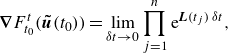
When applying the FTLE to our linear time-periodic system, the deformation gradient of the linearised flow map reads
 \begin{align} \boldsymbol{\nabla} F^t_{t_0}(\boldsymbol{\tilde {u}}(t_0)) =\lim \limits _{\delta t \to 0}\displaystyle \prod _{j=1}^{n} {\rm e}^{{\boldsymbol{L}}(t_j)\,\delta t}, \end{align}
following Farrell & Ioannou (Reference Farrell and Ioannou1996). Here, ${\boldsymbol{L}}(t_j)$
is the linearised operator in (2.4). Note that
${\boldsymbol{L}}(t_j)$
is the linearised operator in (2.4). Note that $\boldsymbol{\nabla} F^t_{t_0}(\boldsymbol{\tilde {u}}(t_0))$
integrates the flow from
$\boldsymbol{\nabla} F^t_{t_0}(\boldsymbol{\tilde {u}}(t_0))$
integrates the flow from $t_0$
to
$t_0$
to $t=t_0 +n\,\delta t$
with
$t=t_0 +n\,\delta t$
with $t_j\in (t_0+(j-1)\,\delta t, t_0+j\,\delta t )$
, and correspondingly, the time-ordering product
$t_j\in (t_0+(j-1)\,\delta t, t_0+j\,\delta t )$
, and correspondingly, the time-ordering product $\Pi$
ensures that the dynamics propagates in the positive temporal direction. To quantify the growth or decay rate of the disturbance as
$\Pi$
ensures that the dynamics propagates in the positive temporal direction. To quantify the growth or decay rate of the disturbance as $t\to \infty$
, the first Lyapunov exponent (Farrell & Ioannou Reference Farrell and Ioannou1996) is defined as
$t\to \infty$
, the first Lyapunov exponent (Farrell & Ioannou Reference Farrell and Ioannou1996) is defined as
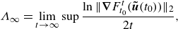 \begin{align} { \Lambda _\infty =\displaystyle \lim _{t\to \infty }\sup \frac {\ln \| \boldsymbol{\nabla} F^t_{t_0}(\boldsymbol{\tilde {u}}(t_0)) \|_2}{2t} }, \end{align}
which implicitly assumes that the disturbance at $t_0$
has a unit norm. A closely related concept is the transient growth, defined as the maximum energy amplification
$t_0$
has a unit norm. A closely related concept is the transient growth, defined as the maximum energy amplification
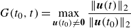 \begin{align} G(t_0, t)=\displaystyle \max _{{\boldsymbol{u}}(t_0)\ne \boldsymbol{0}} \frac {\|\boldsymbol{u}(t)\|_2}{\|\boldsymbol{u}(t_0)\|_2} \end{align}
optimised over all possible initial conditions; see Schmid & Henningson (Reference Schmid and Henningson2001). We will apply the transient growth analysis to the finite Stokes layer. To calculate the maximised energy amplification $G(t_0,t)$
, we follow the direct-adjoint looping algorithm (Luchini & Bottaro Reference Luchini and Bottaro2014), which has also been adopted by Biau (Reference Biau2016). Figure 1(
$G(t_0,t)$
, we follow the direct-adjoint looping algorithm (Luchini & Bottaro Reference Luchini and Bottaro2014), which has also been adopted by Biau (Reference Biau2016). Figure 1( $a$
) validates our calculation in the case
$a$
) validates our calculation in the case $h=16$
against those in the semi-infinite Stokes layer calculated by Biau (Reference Biau2016).
$h=16$
against those in the semi-infinite Stokes layer calculated by Biau (Reference Biau2016).
The Lyapunov exponent $\Lambda _\infty$
at large time (
$\Lambda _\infty$
at large time ( $t\rightarrow \infty$
) is equivalent to the Floquet exponent in a time-periodic system. It concerns the flow behaviour at asymptotically large times. To investigate the intracyclic dynamics in the Stokes layer, we calculate the first FTLE (Shadden Reference Shadden2012; Haller Reference Haller2015)
$t\rightarrow \infty$
) is equivalent to the Floquet exponent in a time-periodic system. It concerns the flow behaviour at asymptotically large times. To investigate the intracyclic dynamics in the Stokes layer, we calculate the first FTLE (Shadden Reference Shadden2012; Haller Reference Haller2015)
 \begin{align} \Lambda (t_0,t) = \sup _{\boldsymbol{u}(t_0)\ne \boldsymbol{0}} \frac {\ln \left ( \dfrac {\| \boldsymbol{u}(t)\|_2}{\| \boldsymbol{u}(t_0)\|_2} \right )}{2(t-t_0)}, \end{align}
with the disturbance initiated at time $t_0$
and evolving until time
$t_0$
and evolving until time $t$
. The FTLE measures the maximum ‘stretching’ effect that a system can have in the time period
$t$
. The FTLE measures the maximum ‘stretching’ effect that a system can have in the time period $[t_0,t]$
. Although it does not directly indicate the growth rate of a perturbation over time, it suggests the potential for maximum transient amplification within the system (Kern et al. Reference Kern, Beneitez, Hanifi and Henningson2021).
$[t_0,t]$
. Although it does not directly indicate the growth rate of a perturbation over time, it suggests the potential for maximum transient amplification within the system (Kern et al. Reference Kern, Beneitez, Hanifi and Henningson2021).
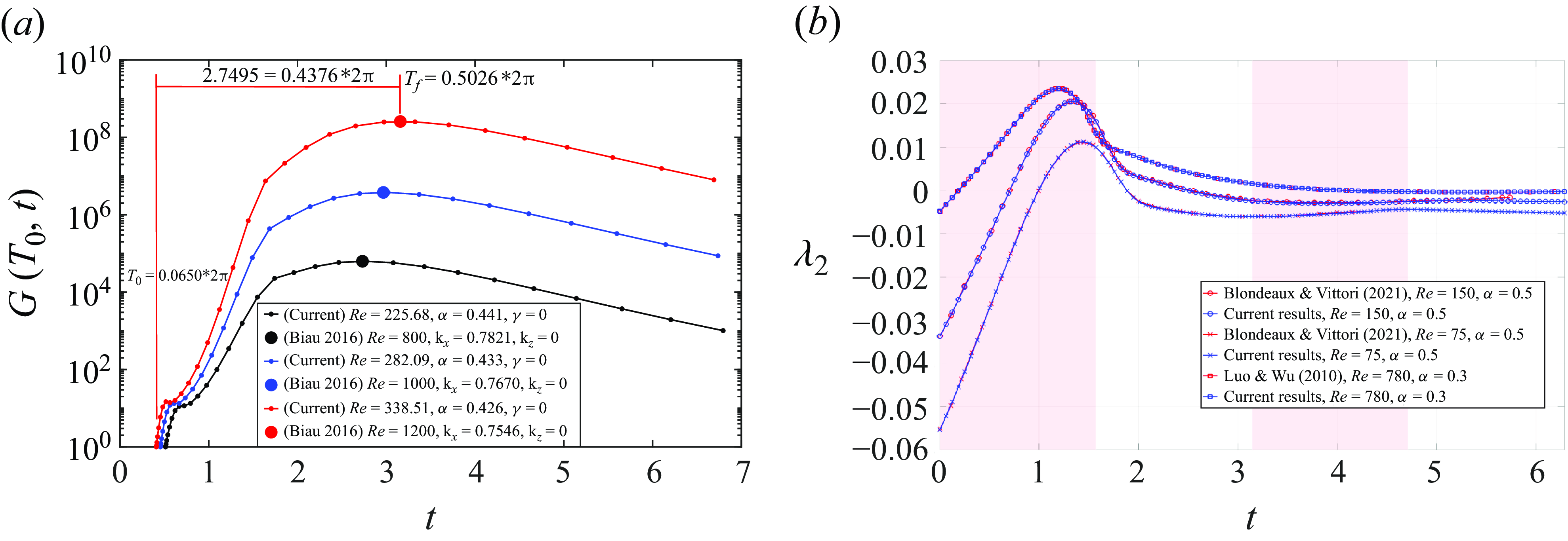
Figure 1. ( $a$
) Transient growth in 2-D Stokes layers with parameters identical to those in Biau (Reference Biau2016). The two studies use different non-dimensionalisation methods for the flow system, necessitating conversion of the parameters; see the legend for details. The finite domain in our computation is set to
$a$
) Transient growth in 2-D Stokes layers with parameters identical to those in Biau (Reference Biau2016). The two studies use different non-dimensionalisation methods for the flow system, necessitating conversion of the parameters; see the legend for details. The finite domain in our computation is set to $h=16$
to mimic the semi-infinite flow considered in Biau (Reference Biau2016). The lines show our computational results, while the three filled dots are extracted from Table 1 of Biau (Reference Biau2016). The
$h=16$
to mimic the semi-infinite flow considered in Biau (Reference Biau2016). The lines show our computational results, while the three filled dots are extracted from Table 1 of Biau (Reference Biau2016). The $T_f$
in Biau (Reference Biau2016) needs to be interpreted as the elapsed time from
$T_f$
in Biau (Reference Biau2016) needs to be interpreted as the elapsed time from $T_0$
, rather than from
$T_0$
, rather than from $0$
, as confirmed by Professor Biau (private communication). Here,
$0$
, as confirmed by Professor Biau (private communication). Here, $T_0$
denotes the starting time in the transient growth calculation, which will later be referred to as
$T_0$
denotes the starting time in the transient growth calculation, which will later be referred to as $t_0$
in our work. (
$t_0$
in our work. ( $b$
) Validation of the 2-D instantaneous/momentary instability analyses against the results in Luo & Wu (Reference Luo and Wu2010) and Blondeaux & Vittori (Reference Blondeaux and Vittori2021). Their results were manually extracted from the respective papers. The red areas represent decelerating phases, and white areas represent accelerating phases.
$b$
) Validation of the 2-D instantaneous/momentary instability analyses against the results in Luo & Wu (Reference Luo and Wu2010) and Blondeaux & Vittori (Reference Blondeaux and Vittori2021). Their results were manually extracted from the respective papers. The red areas represent decelerating phases, and white areas represent accelerating phases.
Existing theories on the instability of Stokes layers include Floquet theory and instantaneous/momentary stability theory, and will also be conducted in this work for comparison. Briefly, Floquet analysis assumes the solution ansatz
 \begin{align} {\boldsymbol{u}}(x,y,z,t) = \displaystyle \left [\sum _{n=-\infty }^\infty {\boldsymbol{u}}^{(n)}(y)\, {\rm e}^{{\rm i}nt}\right ] {\rm e}^{{\rm i}\alpha x + {\rm i}\gamma z -{\rm i}\lambda t}+ \text{c.c.}, \end{align}
where $\lambda$
is the Floquet exponent encompassing the growth/decay rate and frequency of the disturbance, and
$\lambda$
is the Floquet exponent encompassing the growth/decay rate and frequency of the disturbance, and $\text{c.c.}$
indicates the complex conjugate of the preceding term. The infinite Fourier series needs to be truncated in numerical calculation, i.e.
$\text{c.c.}$
indicates the complex conjugate of the preceding term. The infinite Fourier series needs to be truncated in numerical calculation, i.e. $n\in [-N_f,N_f]$
. We consider a sufficient large
$n\in [-N_f,N_f]$
. We consider a sufficient large $N_f$
(
$N_f$
( $\gt 0.8\alpha\, Re$
), following Thomas et al. (Reference Thomas, Bassom, Blennerhassett and Davies2011). Another theory, the instantaneous/momentary stability theory (Luo & Wu Reference Luo and Wu2010; Blondeaux & Vittori Reference Blondeaux and Vittori2021), assumes a solution form that reads
$\gt 0.8\alpha\, Re$
), following Thomas et al. (Reference Thomas, Bassom, Blennerhassett and Davies2011). Another theory, the instantaneous/momentary stability theory (Luo & Wu Reference Luo and Wu2010; Blondeaux & Vittori Reference Blondeaux and Vittori2021), assumes a solution form that reads ${\boldsymbol{u}}(x,y,z,t) = \tilde {\boldsymbol{u}}(y)\exp({{\rm i}\alpha x + {\rm i}\gamma z -{\rm i}\,Re\int \lambda _2(t)\,{\rm d}t})+ \text{c.c.}$
with
${\boldsymbol{u}}(x,y,z,t) = \tilde {\boldsymbol{u}}(y)\exp({{\rm i}\alpha x + {\rm i}\gamma z -{\rm i}\,Re\int \lambda _2(t)\,{\rm d}t})+ \text{c.c.}$
with $\lambda _2$
indicating the stability/instability of the disturbance. Verification of our Floquet analysis of the Stokes layers is shown in table 1, and that of the instantaneous/momentary stability theories in figure 1(
$\lambda _2$
indicating the stability/instability of the disturbance. Verification of our Floquet analysis of the Stokes layers is shown in table 1, and that of the instantaneous/momentary stability theories in figure 1( $b$
).
$b$
).
Table 1. Validation of the 2-D Floquet analysis against the results in Blennerhassett & Bassom (Reference Blennerhassett and Bassom2006) at $\alpha =0.3,\ \gamma =0$
. Even and odd indicate the symmetry of the corresponding least-stable eigenfunction with respect to the channel centreline. We use
$\alpha =0.3,\ \gamma =0$
. Even and odd indicate the symmetry of the corresponding least-stable eigenfunction with respect to the channel centreline. We use $N_y=99$
and
$N_y=99$
and $N_f=170$
for the validation.
$N_f=170$
for the validation.

3. Results and discussion
3.1. General results
Figure 2 shows the comparison of the stability analyses applied to the finite Stokes layer at $Re=540,\ \alpha =0.4,\ \gamma =0,\ h=5$
. This
$Re=540,\ \alpha =0.4,\ \gamma =0,\ h=5$
. This $Re$
is close to values investigated in experiments, e.g. by Akhavan et al. (Reference Akhavan, Kamm and Shapiro1991a
) on the Stokes layer in a pipe, and by Hino et al. (Reference Hino, Kashiwayanagi, Nakayama and Hara1983) on the Stokes layer in a duct (see the caption of figure 3 for details). The streamwise wavenumber
$Re$
is close to values investigated in experiments, e.g. by Akhavan et al. (Reference Akhavan, Kamm and Shapiro1991a
) on the Stokes layer in a pipe, and by Hino et al. (Reference Hino, Kashiwayanagi, Nakayama and Hara1983) on the Stokes layer in a duct (see the caption of figure 3 for details). The streamwise wavenumber $\alpha =0.4$
corresponds closely to the wavelength of the most unstable disturbance, approximately 15, in the nonlinear simulations of Thomas et al. (Reference Thomas, Davies, Bassom and Blennerhassett2014) at
$\alpha =0.4$
corresponds closely to the wavelength of the most unstable disturbance, approximately 15, in the nonlinear simulations of Thomas et al. (Reference Thomas, Davies, Bassom and Blennerhassett2014) at $Re=600$
, which employed the same length scale as ours.
$Re=600$
, which employed the same length scale as ours.
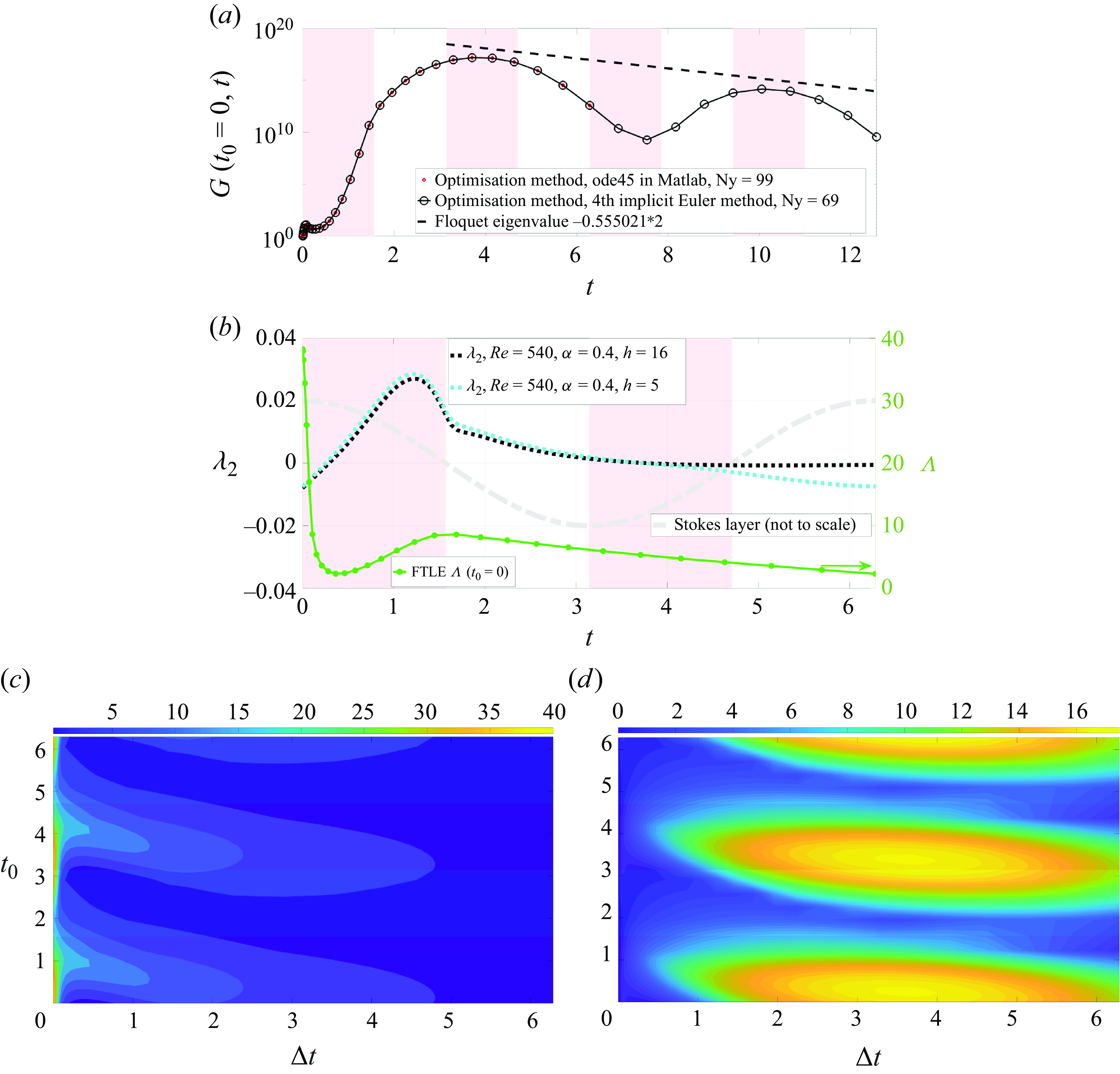
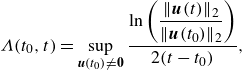
Figure 2. Stability analyses of a typical 2-D finite Stokes layer with $Re=540,\ \alpha =0.4,\ h=5$
. (
$Re=540,\ \alpha =0.4,\ h=5$
. ( $a$
) Transient growth calculated using two time-integration methods (see the legend) and the Floquet decay rate at large time. (
$a$
) Transient growth calculated using two time-integration methods (see the legend) and the Floquet decay rate at large time. ( $b$
) The growth rate
$b$
) The growth rate $\lambda _2$
in the instantaneous/momentary stability analyses (left-hand
$\lambda _2$
in the instantaneous/momentary stability analyses (left-hand $y$
-axis) and the first FTLE
$y$
-axis) and the first FTLE $\Lambda$
(right-hand
$\Lambda$
(right-hand $y$
-axis). (
$y$
-axis). ( $c$
) Distribution of FTLE as a function of the starting time
$c$
) Distribution of FTLE as a function of the starting time $t_0$
and the integrated period
$t_0$
and the integrated period $\Delta t\ (=t-t_0)$
. (d) The corresponding transient growth
$\Delta t\ (=t-t_0)$
. (d) The corresponding transient growth $G(t_0,\Delta t)$
on a base-10 logarithmic scale.
$G(t_0,\Delta t)$
on a base-10 logarithmic scale.
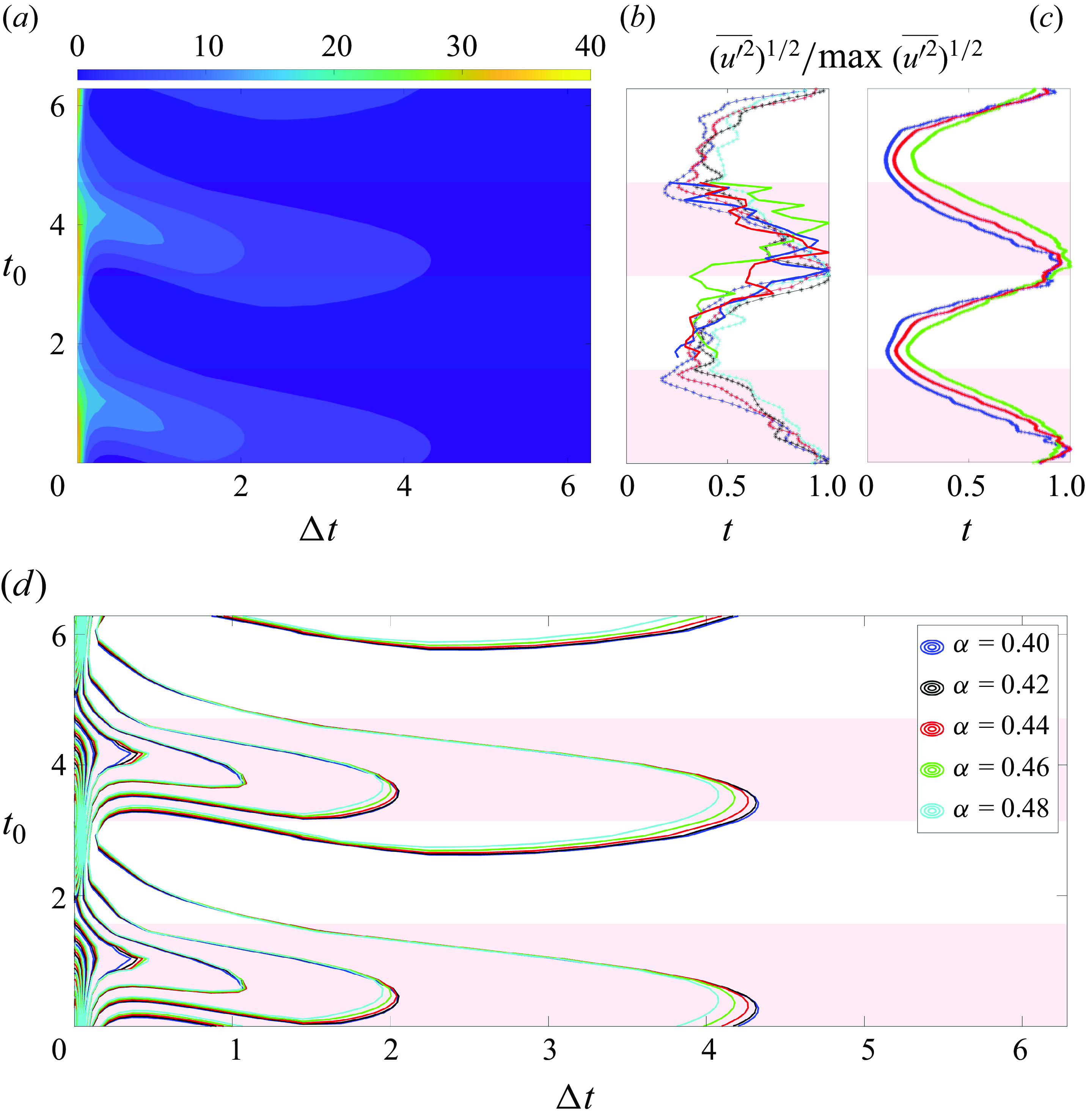
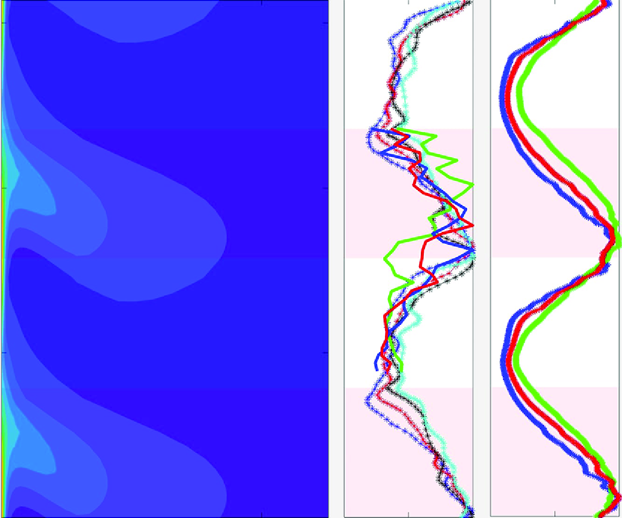
Figure 3. ( $a$
) Distribution of FTLE as function of the starting time
$a$
) Distribution of FTLE as function of the starting time $t_0$
and the integrated period
$t_0$
and the integrated period $\Delta t\ (=t-t_0)$
. The parameters are
$\Delta t\ (=t-t_0)$
. The parameters are $Re=540,\ \alpha =0.4,\ \gamma =0,\ h=10$
. (
$Re=540,\ \alpha =0.4,\ \gamma =0,\ h=10$
. ( $b$
) Normalised axial turbulence intensity
$b$
) Normalised axial turbulence intensity $({\overline {{u'}^2}})^{1/2}$
digitally extracted from the experimental literature. Lines with symbols from figure 9 of Akhavan et al. (Reference Akhavan, Kamm and Shapiro1991a
). Akhavan et al. (Reference Akhavan, Kamm and Shapiro1991a
) concerns the Stokes layer in a pipe with
$({\overline {{u'}^2}})^{1/2}$
digitally extracted from the experimental literature. Lines with symbols from figure 9 of Akhavan et al. (Reference Akhavan, Kamm and Shapiro1991a
). Akhavan et al. (Reference Akhavan, Kamm and Shapiro1991a
) concerns the Stokes layer in a pipe with $Re=540,\ h=10.6$
(or in their notation,
$Re=540,\ h=10.6$
(or in their notation, $Re^\delta =1080,\ \Lambda =10.6$
), and their data are normalised by the maximum value in time at each radial location
$Re^\delta =1080,\ \Lambda =10.6$
), and their data are normalised by the maximum value in time at each radial location $r/R=0.992$
(blue),
$r/R=0.992$
(blue), $0.95$
(red),
$0.95$
(red), $0.85$
(black) and
$0.85$
(black) and $0.75$
(cyan), respectively, where
$0.75$
(cyan), respectively, where $R$
is their pipe radius. Their experimental data have been shifted in time by
$R$
is their pipe radius. Their experimental data have been shifted in time by $\unicode{x03C0} /2$
to be consistent with our wall oscillation signal (i.e.
$\unicode{x03C0} /2$
to be consistent with our wall oscillation signal (i.e. $\cos t$
). Thick lines without symbols from figure 11 of Hino et al. (Reference Hino, Kashiwayanagi, Nakayama and Hara1983). Hino et al. (Reference Hino, Kashiwayanagi, Nakayama and Hara1983) studies the Stokes layer in a duct with
$\cos t$
). Thick lines without symbols from figure 11 of Hino et al. (Reference Hino, Kashiwayanagi, Nakayama and Hara1983). Hino et al. (Reference Hino, Kashiwayanagi, Nakayama and Hara1983) studies the Stokes layer in a duct with $Re=438,\ h=12.8$
(or in their notation,
$Re=438,\ h=12.8$
(or in their notation, $R_\delta =876,\ \lambda =12.8$
), and their data are normalised by the maximum value in time at each vertical location
$R_\delta =876,\ \lambda =12.8$
), and their data are normalised by the maximum value in time at each vertical location $0.01$
(blue),
$0.01$
(blue), $0.05$
(red) and
$0.05$
(red) and $0.1$
(green), respectively, where
$0.1$
(green), respectively, where $d$
is their channel height. (
$d$
is their channel height. ( $c$
) Normalised axial turbulence intensity in our nonlinear simulation (to be detailed in § 3.4). Lines with stars blue curve is for
$c$
) Normalised axial turbulence intensity in our nonlinear simulation (to be detailed in § 3.4). Lines with stars blue curve is for $y=9.9818$
; lines with stars red curve is for
$y=9.9818$
; lines with stars red curve is for $y=9.7773$
; lines with stars green curve is for
$y=9.7773$
; lines with stars green curve is for $y=8.0545$
. (
$y=8.0545$
. ( $d$
) Effect of streamwise wavenumber
$d$
) Effect of streamwise wavenumber $\alpha$
on the first FTLE
$\alpha$
on the first FTLE $\Lambda$
distributed in the
$\Lambda$
distributed in the $t_0{-}\Delta t$
space. The other parameters are the same as those in (a).
$t_0{-}\Delta t$
space. The other parameters are the same as those in (a).
At these parameters, the flow is linearly stable according to the Floquet theory, as indicated by the dashed line in figure 2( $a$
). Figure 2(
$a$
). Figure 2( $b$
) shows that the instantaneous/momentary stability analysis of this flow predicts a negative growth rate
$b$
) shows that the instantaneous/momentary stability analysis of this flow predicts a negative growth rate $\lambda _2$
at the beginning of the first deceleration phase (red shade). For the chosen parameters, this contradicts the experimental observation that ‘turbulence appeared explosively towards the end of the acceleration phase of the cycle and was sustained throughout the deceleration phase’ (Akhavan et al. Reference Akhavan, Kamm and Shapiro1991a
).
$\lambda _2$
at the beginning of the first deceleration phase (red shade). For the chosen parameters, this contradicts the experimental observation that ‘turbulence appeared explosively towards the end of the acceleration phase of the cycle and was sustained throughout the deceleration phase’ (Akhavan et al. Reference Akhavan, Kamm and Shapiro1991a
).
Conversely, the transient growth $G(t_0=0,t)$
in figure 2(
$G(t_0=0,t)$
in figure 2( $a$
) initially shows a quick increase around
$a$
) initially shows a quick increase around $t=0$
and further climbs to
$t=0$
and further climbs to $10^{17}$
in the second decelerating phase at
$10^{17}$
in the second decelerating phase at $t\approx 4$
. The substantial transient growth is consistent with the calculation by Biau (Reference Biau2016) for the semi-infinite Stokes layer, and the significant flow response to an impulse excitation studied by Thomas et al. (Reference Thomas, Davies, Bassom and Blennerhassett2014) (cf. their figure 1). The mechanical explanation for this 2-D transient growth has been attributed to the Orr mechanism by Biau (Reference Biau2016). Biau also confirmed that three-dimensional (3-D) transient growth is less significant than its 2-D counterpart. Given that the maximum transient growth is exceptionally large, even small systematic or external perturbations may be amplified appreciably. This may explain why no experiments have reported carefully controlled Stokes layers reaching a supercritical transition. In short, despite the Floquet stability of the Stokes layer, a subcritical transition likely occurs.
$t\approx 4$
. The substantial transient growth is consistent with the calculation by Biau (Reference Biau2016) for the semi-infinite Stokes layer, and the significant flow response to an impulse excitation studied by Thomas et al. (Reference Thomas, Davies, Bassom and Blennerhassett2014) (cf. their figure 1). The mechanical explanation for this 2-D transient growth has been attributed to the Orr mechanism by Biau (Reference Biau2016). Biau also confirmed that three-dimensional (3-D) transient growth is less significant than its 2-D counterpart. Given that the maximum transient growth is exceptionally large, even small systematic or external perturbations may be amplified appreciably. This may explain why no experiments have reported carefully controlled Stokes layers reaching a supercritical transition. In short, despite the Floquet stability of the Stokes layer, a subcritical transition likely occurs.
To investigate the intracyclic instability in the Stokes layer from the lens of the FTLE, the first FTLE $\Lambda$
is computed and shown in figure 2(
$\Lambda$
is computed and shown in figure 2( $b$
) with
$b$
) with $t_0=0$
as a function of
$t_0=0$
as a function of $t$
. The result for
$t$
. The result for $\Lambda$
presents a different trend than
$\Lambda$
presents a different trend than $\lambda _2$
in the instantaneous/momentary stability analysis, and approaches the negative Floquet exponent
$\lambda _2$
in the instantaneous/momentary stability analysis, and approaches the negative Floquet exponent $\lambda$
as
$\lambda$
as $t\to \infty$
in this case. Figure 2(
$t\to \infty$
in this case. Figure 2( $d$
) shows the corresponding
$d$
) shows the corresponding $G(t_0,\Delta t)$
on a base-10 logarithmic scale. It can be seen that the global maximum transient growth is found at approximately
$G(t_0,\Delta t)$
on a base-10 logarithmic scale. It can be seen that the global maximum transient growth is found at approximately $\Delta t\in [3,4]$
after the initial disturbance is imposed. Besides, the global maximum transient growth takes place in the decelerating phases (see the red areas), which is an encouraging result.
$\Delta t\in [3,4]$
after the initial disturbance is imposed. Besides, the global maximum transient growth takes place in the decelerating phases (see the red areas), which is an encouraging result.
3.2. The FTLE results compared to experiments
The focus of the work is to test the comparison of the FTLE and transient growth with the experimentally observed intracyclic instability in the Stokes layer flow. An appealing comparison of the FTLE with the experimental data is shown in figure 3( $a$
), which presents the distribution of
$a$
), which presents the distribution of $\Lambda$
as a function
$\Lambda$
as a function $t_0$
and
$t_0$
and $\Delta t\ (= t-t_0)$
. We now take
$\Delta t\ (= t-t_0)$
. We now take $h=10$
to be consistent with the experimental set-up (see the caption for details). Overall, the distribution implies relatively larger growth rates during the decelerating phases (red shades in the contour figure), indicating stronger flow instability, which may lead to more intensive turbulence. This appears to be consistent with the experimental observation that strong turbulent activity bursts and persists in the decelerating phases, but weaker turbulence occurs during the accelerating phase; see figure 9 in Akhavan et al. (Reference Akhavan, Kamm and Shapiro1991a
) for the turbulence intensity, figure 6 in Hino, Sawamoto & Takasu (Reference Hino, Sawamoto and Takasu1976) for the velocity variation, and figures 15 and 16 in Hino et al. (Reference Hino, Kashiwayanagi, Nakayama and Hara1983) for the turbulence energy production. As pointed out by one of the reviewers, the experiments were conducted with oscillating pressure gradient and stationary walls. Indeed, conducting experiments with physically oscillating walls is not practically feasible. However, from a mathematical standpoint, the Navier–Stokes equations with oscillating wall boundary conditions are equivalent to those with an oscillating pressure gradient and stationary walls. Therefore, it is reasonable to compare our results directly with the existing experiments involving oscillatory pressure-driven flows.
$h=10$
to be consistent with the experimental set-up (see the caption for details). Overall, the distribution implies relatively larger growth rates during the decelerating phases (red shades in the contour figure), indicating stronger flow instability, which may lead to more intensive turbulence. This appears to be consistent with the experimental observation that strong turbulent activity bursts and persists in the decelerating phases, but weaker turbulence occurs during the accelerating phase; see figure 9 in Akhavan et al. (Reference Akhavan, Kamm and Shapiro1991a
) for the turbulence intensity, figure 6 in Hino, Sawamoto & Takasu (Reference Hino, Sawamoto and Takasu1976) for the velocity variation, and figures 15 and 16 in Hino et al. (Reference Hino, Kashiwayanagi, Nakayama and Hara1983) for the turbulence energy production. As pointed out by one of the reviewers, the experiments were conducted with oscillating pressure gradient and stationary walls. Indeed, conducting experiments with physically oscillating walls is not practically feasible. However, from a mathematical standpoint, the Navier–Stokes equations with oscillating wall boundary conditions are equivalent to those with an oscillating pressure gradient and stationary walls. Therefore, it is reasonable to compare our results directly with the existing experiments involving oscillatory pressure-driven flows.
To facilitate the comparison, the experimental results of axial turbulence intensity extracted from Akhavan et al. (Reference Akhavan, Kamm and Shapiro1991a
) and Hino et al. (Reference Hino, Kashiwayanagi, Nakayama and Hara1983) are reproduced in figure 3(b) at various radial/vertical locations in their experiments. Notably, the ‘eggplant’ regions within $\Delta t \in [1, 2\unicode{x03C0} ]$
in our
$\Delta t \in [1, 2\unicode{x03C0} ]$
in our $\Lambda$
distribution, which encompass the maximum transient growth, precisely align with the peak positions of axial turbulence intensity observed in the experiments. Figure 3(
$\Lambda$
distribution, which encompass the maximum transient growth, precisely align with the peak positions of axial turbulence intensity observed in the experiments. Figure 3( $c$
) shows the results of our nonlinear simulations, which will be discussed in detail in § 3.4. As a brief remark, the intracyclic instability observed in the nonlinear simulations is also consistent with the FTLE results. In short, figures 3(a,b) reveals a strong correlation between the distribution of the FTLE and the experimentally observed axial turbulence intensity, providing convincing evidence of intracyclic dynamics in the finite Stokes layer. Together with Biau (Reference Biau2016), these results imply a linear energy amplification mechanism underpinning the turbulence generation cycle in transitional Stokes layers.
$c$
) shows the results of our nonlinear simulations, which will be discussed in detail in § 3.4. As a brief remark, the intracyclic instability observed in the nonlinear simulations is also consistent with the FTLE results. In short, figures 3(a,b) reveals a strong correlation between the distribution of the FTLE and the experimentally observed axial turbulence intensity, providing convincing evidence of intracyclic dynamics in the finite Stokes layer. Together with Biau (Reference Biau2016), these results imply a linear energy amplification mechanism underpinning the turbulence generation cycle in transitional Stokes layers.
The above result focuses on the Stokes layer for a single wavelength. To assess the robustness of the FTLE distribution across different wavelengths, figure 3( $d$
) presents line contours of the FTLE for
$d$
) presents line contours of the FTLE for $\alpha =0.40:0.02:0.48$
. This range of
$\alpha =0.40:0.02:0.48$
. This range of $\alpha$
encompasses the most significant transient growth in this subcritical Stokes layer; see also figure 4. The same FTLE distribution is observed across all these wavenumbers, demonstrating that the energy amplification mechanism in the finite Stokes layer extends over a spectrum of wavenumbers linked to the most amplified disturbances.
$\alpha$
encompasses the most significant transient growth in this subcritical Stokes layer; see also figure 4. The same FTLE distribution is observed across all these wavenumbers, demonstrating that the energy amplification mechanism in the finite Stokes layer extends over a spectrum of wavenumbers linked to the most amplified disturbances.

Figure 4. Effect of $\alpha$
and
$\alpha$
and $Re$
on the transient growth
$Re$
on the transient growth $G(t_0=0,t)$
(colour contour) in 2-D finite Stokes layers with
$G(t_0=0,t)$
(colour contour) in 2-D finite Stokes layers with $h=5$
.
$h=5$
.
3.3. Parametric study: effects of $Re$
,
$h$
and
$\omega$
$Re$
,
$h$
and
$\omega$


A parametric study of the effects of $Re$
and
$Re$
and $\alpha$
on the transient growth
$\alpha$
on the transient growth $G(t_0=0,t)$
in the 2-D finite Stokes layer is shown in figure 4. It is evident that transient growth rises with
$G(t_0=0,t)$
in the 2-D finite Stokes layer is shown in figure 4. It is evident that transient growth rises with $Re$
within this subcritical range. This is consistent with the calculation by Biau (Reference Biau2016), who similarly observed the monotonic increases of the transient growth in the subcritical semi-infinite Stokes layer. The optimal wavenumber for transient growth is found to be approximately
$Re$
within this subcritical range. This is consistent with the calculation by Biau (Reference Biau2016), who similarly observed the monotonic increases of the transient growth in the subcritical semi-infinite Stokes layer. The optimal wavenumber for transient growth is found to be approximately $\alpha = 0.42$
, thereby supporting our choice of
$\alpha = 0.42$
, thereby supporting our choice of $\alpha = 0.4$
in the present investigation.
$\alpha = 0.4$
in the present investigation.
Next, we explore the effect of the half-wall distance $h$
on the FTLE in the finite Stokes layers. Large-
$h$
on the FTLE in the finite Stokes layers. Large- $h$
flows have been widely studied in the literature, while small-
$h$
flows have been widely studied in the literature, while small- $h$
cases, though less explored, are relevant in fields such as biology and microrheology (Mitran et al. Reference Mitran, Forest, Yao, Lindley and Hill2008). Figure 5(
$h$
cases, though less explored, are relevant in fields such as biology and microrheology (Mitran et al. Reference Mitran, Forest, Yao, Lindley and Hill2008). Figure 5( $a$
) shows the 2-D transient growth at
$a$
) shows the 2-D transient growth at $Re=540,\ \alpha =0.4$
for various
$Re=540,\ \alpha =0.4$
for various $h$
. For relatively large
$h$
. For relatively large $h$
(
$h$
( $h\geqslant 9$
), the flow resembles its semi-infinite counterpart, presenting significant transient growth. The effect of changing
$h\geqslant 9$
), the flow resembles its semi-infinite counterpart, presenting significant transient growth. The effect of changing $h$
is minor in this range. The maximum
$h$
is minor in this range. The maximum $G(t_0=0,t)$
is found at
$G(t_0=0,t)$
is found at $h=5$
; see the magenta line. Upon reducing
$h=5$
; see the magenta line. Upon reducing $h$
, the transient growth decreases drastically. This suggests that as
$h$
, the transient growth decreases drastically. This suggests that as $h$
decreases, the linear amplification mechanism weakens. This trend is consistent with the observation by Hino et al. (Reference Hino, Sawamoto and Takasu1976) that ‘The critical Reynolds number of the first transition decreases as the Stokes parameter increases’ in the small-
$h$
decreases, the linear amplification mechanism weakens. This trend is consistent with the observation by Hino et al. (Reference Hino, Sawamoto and Takasu1976) that ‘The critical Reynolds number of the first transition decreases as the Stokes parameter increases’ in the small- $h$
range. Their Stokes parameter is identified as
$h$
range. Their Stokes parameter is identified as $h$
in our work. To illustrate the feature of the
$h$
in our work. To illustrate the feature of the $\Lambda$
distribution in the small-
$\Lambda$
distribution in the small- $h$
Stokes layers, we take the case
$h$
Stokes layers, we take the case $h = 2$
as an example, depicted in figure 5(
$h = 2$
as an example, depicted in figure 5( $b$
). By comparing this result with that for
$b$
). By comparing this result with that for $h=10$
in figure 3 and that for
$h=10$
in figure 3 and that for $h=5$
in figure 2 (corresponding to the maximum FTLE over all
$h=5$
in figure 2 (corresponding to the maximum FTLE over all $h$
), it is evident that the FTLE for
$h$
), it is evident that the FTLE for $h=2$
is significantly smaller and exhibits a weaker history effect along the
$h=2$
is significantly smaller and exhibits a weaker history effect along the $\Delta t$
-axis. Thus our FTLE analysis suggests a weaker energy amplification mechanism in the small-
$\Delta t$
-axis. Thus our FTLE analysis suggests a weaker energy amplification mechanism in the small- $h$
Stokes layers. Based on this observation, we hypothesise that the small-
$h$
Stokes layers. Based on this observation, we hypothesise that the small- $h$
Stokes layers, if they can transition to turbulence, will show a smaller temporal standard deviation in the normalised axial turbulence intensity, compared to the large-
$h$
Stokes layers, if they can transition to turbulence, will show a smaller temporal standard deviation in the normalised axial turbulence intensity, compared to the large- $h$
flows. We encourage future experimental research to confirm this finding by changing the dimensional channel half-height
$h$
flows. We encourage future experimental research to confirm this finding by changing the dimensional channel half-height $d$
.
$d$
.

Figure 5. ( $a$
) Effect of non-dimensional channel half-height
$a$
) Effect of non-dimensional channel half-height $h$
on the transient growth
$h$
on the transient growth $G(t_0=0,t)$
. (
$G(t_0=0,t)$
. ( $b$
) Distribution of the first FTLE
$b$
) Distribution of the first FTLE $\Lambda$
in the
$\Lambda$
in the $t_0{-}\Delta t$
plane for the case
$t_0{-}\Delta t$
plane for the case $h=2$
. The other parameters are
$h=2$
. The other parameters are $Re=540,\ \alpha =0.4,\ \gamma =0$
.
$Re=540,\ \alpha =0.4,\ \gamma =0$
.
In experiments involving the Stokes layer, nevertheless, the most practical way to vary the system parameters is by adjusting the wall-oscillation frequency $\omega$
. Under our non-dimensionalisation scheme, changes in
$\omega$
. Under our non-dimensionalisation scheme, changes in $\omega$
induce corresponding changes in
$\omega$
induce corresponding changes in $Re$
,
$Re$
, $h$
and
$h$
and $\alpha$
. To investigate how transient growth varies with frequency, we consider a reference parameter set defined by
$\alpha$
. To investigate how transient growth varies with frequency, we consider a reference parameter set defined by
 \begin{align} { Re_{\textit{ref}} = \frac {U_0}{\sqrt {2\nu \omega _{\textit{ref}}}} = 540\quad \text{and}\quad h_{\textit{ref}} = \frac {d}{\sqrt {2\nu / \omega _{\textit{ref}}}} = 3, } \end{align}
while fixing $\alpha _{\textit{ref}} = 0.4$
. We choose to fix
$\alpha _{\textit{ref}} = 0.4$
. We choose to fix $\alpha = 0.4$
because in realistic experiments, a spectrum of waves is typically excited rather than a single mode. Our parametric study (see figure 4) indicates that the maximum transient growth occurs near
$\alpha = 0.4$
because in realistic experiments, a spectrum of waves is typically excited rather than a single mode. Our parametric study (see figure 4) indicates that the maximum transient growth occurs near $\alpha \approx 0.4$
, justifying its use to focus on the most dangerous scenario. Defining the frequency ratio as
$\alpha \approx 0.4$
, justifying its use to focus on the most dangerous scenario. Defining the frequency ratio as $r = \omega / \omega _{\textit{ref}}$
, the new dimensionless parameters become
$r = \omega / \omega _{\textit{ref}}$
, the new dimensionless parameters become
 \begin{align} { Re = \frac {Re_{\textit{ref}}}{\sqrt {r}}, \quad h = h_{\textit{ref}}\, \sqrt {r} } \end{align}
as functions of $r$
.
$r$
.
Figure 6 implies that increasing $\omega$
(or equivalently
$\omega$
(or equivalently $r$
) leads to a non-monotonic response in the maximum transient growth, with the initial disturbance imposed at
$r$
) leads to a non-monotonic response in the maximum transient growth, with the initial disturbance imposed at $t_0=0$
. From
$t_0=0$
. From $r=0.5$
(
$r=0.5$
( $h = 2.1213,\ Re=763.7$
) to
$h = 2.1213,\ Re=763.7$
) to $r=1$
(
$r=1$
( $h = 3,\ Re=540$
), the maximum transient growth increases, indicating a destabilising effect of increasing frequency. Beyond this point, however, further increases in frequency suppress transient growth. We compare this trend to those in the literature. Merkli & Thomann (Reference Merkli and Thomann1975) showed in their figure 5 that the maximum velocity in the flow increases with increasing frequency, suggesting a destabilising effect associated with higher oscillation frequencies. The discrepancy between our results and those of Merkli & Thomann (Reference Merkli and Thomann1975) may arise from differences in the parameter regimes explored. As presented in our figure 5, the value of
$h = 3,\ Re=540$
), the maximum transient growth increases, indicating a destabilising effect of increasing frequency. Beyond this point, however, further increases in frequency suppress transient growth. We compare this trend to those in the literature. Merkli & Thomann (Reference Merkli and Thomann1975) showed in their figure 5 that the maximum velocity in the flow increases with increasing frequency, suggesting a destabilising effect associated with higher oscillation frequencies. The discrepancy between our results and those of Merkli & Thomann (Reference Merkli and Thomann1975) may arise from differences in the parameter regimes explored. As presented in our figure 5, the value of $h$
seems to be playing an important role in determining the transient growth; however, Merkli & Thomann (Reference Merkli and Thomann1975) did not report the values of
$h$
seems to be playing an important role in determining the transient growth; however, Merkli & Thomann (Reference Merkli and Thomann1975) did not report the values of $h$
, making a direct comparison difficult.
$h$
, making a direct comparison difficult.
To gain further insight, we refer to the experimental work of Hino et al. (Reference Hino, Sawamoto and Takasu1976), where a comparable parameter $\lambda$
(the same definition as our
$\lambda$
(the same definition as our $h$
) increases from 2.76 to 3.90 as the oscillation period
$h$
) increases from 2.76 to 3.90 as the oscillation period $T$
is reduced from 6.0 s to 3.0 s, effectively doubling the frequency. Table 1 of Hino et al. (Reference Hino, Sawamoto and Takasu1976) shows that the increase in
$T$
is reduced from 6.0 s to 3.0 s, effectively doubling the frequency. Table 1 of Hino et al. (Reference Hino, Sawamoto and Takasu1976) shows that the increase in $\lambda$
is accompanied by a transition from disturbed laminar flow (denoted by empty circles) to weak turbulence (denoted by filled circles), also supporting the destabilising effect of increasing frequency. Notably, this transition in experiments occurs within the range
$\lambda$
is accompanied by a transition from disturbed laminar flow (denoted by empty circles) to weak turbulence (denoted by filled circles), also supporting the destabilising effect of increasing frequency. Notably, this transition in experiments occurs within the range $h \in [2.76, 3.90]$
, which approximately aligns with the low-
$h \in [2.76, 3.90]$
, which approximately aligns with the low- $h$
regime in our study, where a similar destabilising trend is observed.
$h$
regime in our study, where a similar destabilising trend is observed.

Figure 6. Contour plot of $G(t_0 = 0, t)$
on a base-10 logarithmic scale. The left-hand
$G(t_0 = 0, t)$
on a base-10 logarithmic scale. The left-hand $y$
-axis indicates the ratio
$y$
-axis indicates the ratio $\omega / \omega _{\textit{ref}}$
, where
$\omega / \omega _{\textit{ref}}$
, where $\omega _{\textit{ref}}$
corresponds to the reference parameter set
$\omega _{\textit{ref}}$
corresponds to the reference parameter set $(Re_{\textit{ref}} = 540,\ h_{\textit{ref}} = 3)$
. The wavenumber is fixed at
$(Re_{\textit{ref}} = 540,\ h_{\textit{ref}} = 3)$
. The wavenumber is fixed at $\alpha = 0.4$
in all cases, to capture the most amplified transient growth. The corresponding values of
$\alpha = 0.4$
in all cases, to capture the most amplified transient growth. The corresponding values of $h$
and
$h$
and $Re$
are also shown in blue and red, respectively.
$Re$
are also shown in blue and red, respectively.
3.4. Nonlinear evolution
The discussions above centre around the linear dynamics. To further extend the implication of the linear results, especially the intracyclic instability shown in figure 3, nonlinear simulations were conducted. The numerical method adopted is the classic peusdo-spectral method, and the details are presented in Appendix A. The computation domain, with the channel half-height as the reference length, is ( $2\unicode{x03C0} /0.4, 5, 2\unicode{x03C0}$
) discretised with resolution
$2\unicode{x03C0} /0.4, 5, 2\unicode{x03C0}$
) discretised with resolution $129\times 105\times 89$
along the
$129\times 105\times 89$
along the $x,y,z$
directions. A constant time step
$x,y,z$
directions. A constant time step ${\rm d}t= 2\unicode{x03C0} /2\,50\,000\approx 2.5132\times 10^{-5}$
is considered. The initial condition of the nonlinear simulation consists of the laminar Stokes layer solution at
${\rm d}t= 2\unicode{x03C0} /2\,50\,000\approx 2.5132\times 10^{-5}$
is considered. The initial condition of the nonlinear simulation consists of the laminar Stokes layer solution at $t=0$
plus the optimal initial condition (whose kinetic energy is
$t=0$
plus the optimal initial condition (whose kinetic energy is $10^{-10}$
) targeting the maximum transient growth at
$10^{-10}$
) targeting the maximum transient growth at $t=1$
. A 3-D perturbation is additionally imposed to trigger the transition, following Biau (Reference Biau2016).
$t=1$
. A 3-D perturbation is additionally imposed to trigger the transition, following Biau (Reference Biau2016).
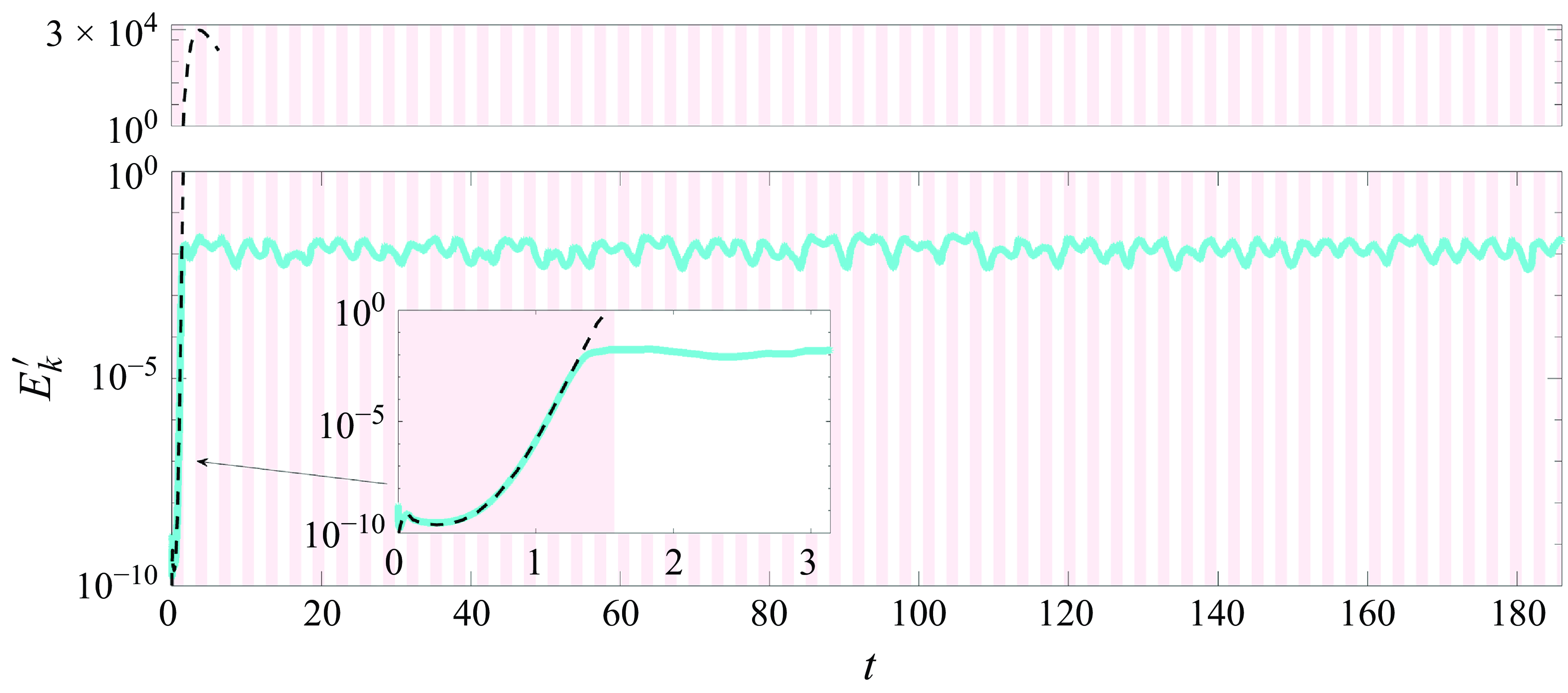
Figure 7. Nonlinear evolution of the perturbation kinetic energy $E'_k(t) = ({1}/{2h})\int \|{\boldsymbol{u}}(y,t) - {\boldsymbol{U}}_b(y,t) \|^2\, {\rm d}y$
(cyan line) at
$E'_k(t) = ({1}/{2h})\int \|{\boldsymbol{u}}(y,t) - {\boldsymbol{U}}_b(y,t) \|^2\, {\rm d}y$
(cyan line) at $Re=540,\ h=10$
. Note that
$Re=540,\ h=10$
. Note that ${\boldsymbol{u}}(y,t)$
have been averaged over the
${\boldsymbol{u}}(y,t)$
have been averaged over the $x{-}z$
plane before the integration, and
$x{-}z$
plane before the integration, and ${\boldsymbol{U}}_b(y,t)$
is homogeneous in the
${\boldsymbol{U}}_b(y,t)$
is homogeneous in the $x{-}z$
plane by definition. The dashed black line represents the envelope of the maximum transient growth. The total simulation time is approximately 186 time units, corresponding to 29.6 complete periods.
$x{-}z$
plane by definition. The dashed black line represents the envelope of the maximum transient growth. The total simulation time is approximately 186 time units, corresponding to 29.6 complete periods.
Figure 7 presents the evolution of the perturbation energy $ E'_k$
, computed by integrating the kinetic energy of the velocity deviation from the laminar Stokes layer solution
$ E'_k$
, computed by integrating the kinetic energy of the velocity deviation from the laminar Stokes layer solution ${\boldsymbol{U}}_b(y,t)$
over the entire domain at
${\boldsymbol{U}}_b(y,t)$
over the entire domain at $ Re = 540$
. The inset highlights that the evolution of
$ Re = 540$
. The inset highlights that the evolution of $ E'_k$
closely follows the optimal growth envelope (calculated in the transient growth analysis), indicated by the black dashed line; this is an outcome of the optimal initial condition as part of the initial condition used in our nonlinear simulation. The sharp energy rise at
$ E'_k$
closely follows the optimal growth envelope (calculated in the transient growth analysis), indicated by the black dashed line; this is an outcome of the optimal initial condition as part of the initial condition used in our nonlinear simulation. The sharp energy rise at $ t = 0$
results from the 3-D disturbance, which decays rapidly. After the initial transient, the flow reaches a statistically saturated state before the end of the first decelerating phase. It is evident that the perturbation energy consistently troughs during the accelerating phases (white background) and peaks during the decelerating phases (red shading). This behaviour aligns with both the FTLE analysis and the experimental observations shown in figures 3(a,b). To enable a more quantitative comparison, we also compute the phase-averaged axial turbulence intensity
$ t = 0$
results from the 3-D disturbance, which decays rapidly. After the initial transient, the flow reaches a statistically saturated state before the end of the first decelerating phase. It is evident that the perturbation energy consistently troughs during the accelerating phases (white background) and peaks during the decelerating phases (red shading). This behaviour aligns with both the FTLE analysis and the experimental observations shown in figures 3(a,b). To enable a more quantitative comparison, we also compute the phase-averaged axial turbulence intensity $ ({\overline {u'^2}})^{1/2}$
, normalised by its maximum value, at three different vertical positions (
$ ({\overline {u'^2}})^{1/2}$
, normalised by its maximum value, at three different vertical positions ( $y=9.9818, 9.7773, 8.0545$
) approximately corresponding to the three vertical positions in Hino et al. (Reference Hino, Kashiwayanagi, Nakayama and Hara1983); see the lines with stars curves in figure 3(
$y=9.9818, 9.7773, 8.0545$
) approximately corresponding to the three vertical positions in Hino et al. (Reference Hino, Kashiwayanagi, Nakayama and Hara1983); see the lines with stars curves in figure 3( $c$
). The axial turbulence intensity is calculated by subtracting the axial component of the laminar Stokes layer
$c$
). The axial turbulence intensity is calculated by subtracting the axial component of the laminar Stokes layer ${{U}}_b(y,t)$
from the raw data. The result in figure 3(
${{U}}_b(y,t)$
from the raw data. The result in figure 3( $c$
) confirms that the phase evolution of axial turbulence intensity relative to the laminar reference flow qualitatively captures the intracyclic instability of the perturbations.
$c$
) confirms that the phase evolution of axial turbulence intensity relative to the laminar reference flow qualitatively captures the intracyclic instability of the perturbations.
As nonlinear effects distort the laminar base flow, it is instructive to compare the laminar Stokes layer ${\boldsymbol{U}}_b(y,t)$
with the phase-averaged flow, denoted as
${\boldsymbol{U}}_b(y,t)$
with the phase-averaged flow, denoted as $\bar {\boldsymbol{u}}(y,t)$
averaged over the
$\bar {\boldsymbol{u}}(y,t)$
averaged over the $x{-}z$
plane. The
$x{-}z$
plane. The $x$
component of the two flows is shown in figure 8. The nonlinear simulation was run for 186 time units, corresponding to 29.6 oscillation periods. To eliminate initial transients, the first two periods are discarded, leaving the remaining 27 periods to be used for the phase averaging. This duration is considered sufficiently long, comparable with simulation times reported in studies such as 2–13 cycles in Vittori & Verzicco (Reference Vittori and Verzicco1998), 50 cycles in Manna, Vacca & Verzicco (Reference Manna, Vacca and Verzicco2015), and 10 cycles in Ebadi et al. (Reference Ebadi, White, Pond and Dubief2019). Figure 8(a) displays the laminar Stokes layer in a
$x$
component of the two flows is shown in figure 8. The nonlinear simulation was run for 186 time units, corresponding to 29.6 oscillation periods. To eliminate initial transients, the first two periods are discarded, leaving the remaining 27 periods to be used for the phase averaging. This duration is considered sufficiently long, comparable with simulation times reported in studies such as 2–13 cycles in Vittori & Verzicco (Reference Vittori and Verzicco1998), 50 cycles in Manna, Vacca & Verzicco (Reference Manna, Vacca and Verzicco2015), and 10 cycles in Ebadi et al. (Reference Ebadi, White, Pond and Dubief2019). Figure 8(a) displays the laminar Stokes layer in a $y$
–
$y$
– $t$
diagram, and figure 8(b) shows the phase-averaged flow. Although the near-wall velocity patterns appear similar in the two flows, the less tilted green/cyan stripes in the
$t$
diagram, and figure 8(b) shows the phase-averaged flow. Although the near-wall velocity patterns appear similar in the two flows, the less tilted green/cyan stripes in the ${\bar {u}}(y,t)$
field suggest enhanced temporal coherence across the velocity field. The small difference, as shown in figure 8(c), indicates the relative resemblance of the two flows.
${\bar {u}}(y,t)$
field suggest enhanced temporal coherence across the velocity field. The small difference, as shown in figure 8(c), indicates the relative resemblance of the two flows.
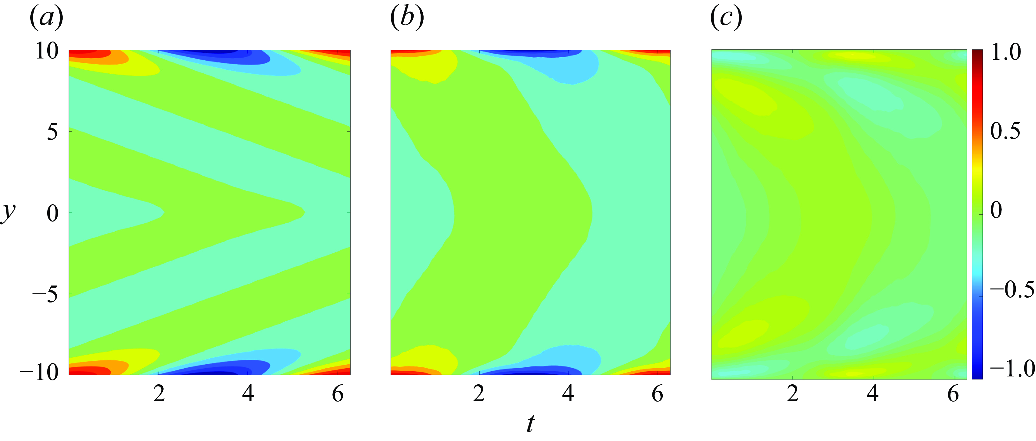
Figure 8. Profiles of (a) the laminar Stokes layer ${{U}}_b(y,t)$
, (b) the phase-averaged flow along the
${{U}}_b(y,t)$
, (b) the phase-averaged flow along the $x$
direction over 27 periods
$x$
direction over 27 periods ${\bar {u}}(y,t)$
, and (c) the difference between the two,
${\bar {u}}(y,t)$
, and (c) the difference between the two, ${{U}}_b(y,t)-{\bar {u}}(y,t)$
, at
${{U}}_b(y,t)-{\bar {u}}(y,t)$
, at $Re=540,\ h=10$
. Here,
$Re=540,\ h=10$
. Here, ${\bar {u}}(y,t)$
has been spatially averaged in the
${\bar {u}}(y,t)$
has been spatially averaged in the $x{-}z$
plane.
$x{-}z$
plane.
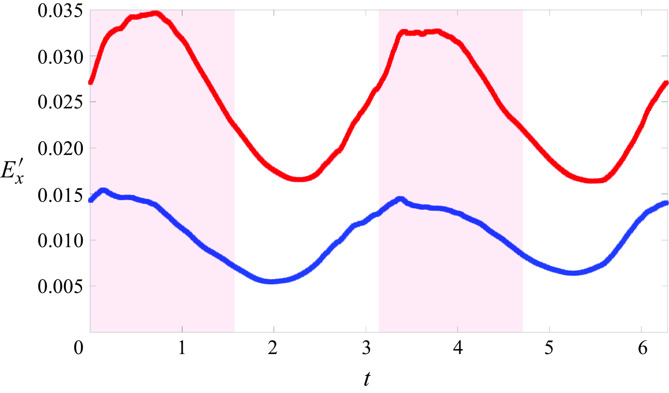
Figure 9. Phase-averaged $x$
component perturbation kinetic energy
$x$
component perturbation kinetic energy $E'_x(t)$
calculated with respect to the laminar flow (red,
$E'_x(t)$
calculated with respect to the laminar flow (red, $E'_x(t) = ({1}/{2h})\int \|{{u}}(y,t) - {{U}}_b(y,t) \|^2\, {\rm d}y$
) and the time-mean flow (blue,
$E'_x(t) = ({1}/{2h})\int \|{{u}}(y,t) - {{U}}_b(y,t) \|^2\, {\rm d}y$
) and the time-mean flow (blue, $E'_x(t) = ({1}/{2h})\int \|{{u}}(y,t) - {\bar {u}}(y,t) \|^2\, {\rm d}y$
) at
$E'_x(t) = ({1}/{2h})\int \|{{u}}(y,t) - {\bar {u}}(y,t) \|^2\, {\rm d}y$
) at $Re=540,\ h=10$
. Here,
$Re=540,\ h=10$
. Here, ${\bar {u}}(y,t)$
denotes the
${\bar {u}}(y,t)$
denotes the $x$
component of the phase-averaged flow, averaged over the
$x$
component of the phase-averaged flow, averaged over the $x{-}z$
plane.
$x{-}z$
plane.
To further compare the laminar base flow ${\boldsymbol{U}}_b(y,t)$
and the phase-averaged flow
${\boldsymbol{U}}_b(y,t)$
and the phase-averaged flow $\bar {\boldsymbol{u}}(y,t)$
, figure 9 shows the
$\bar {\boldsymbol{u}}(y,t)$
, figure 9 shows the $x$
component of the perturbation kinetic energy
$x$
component of the perturbation kinetic energy $ E'_x$
computed with respect to them. As observed,
$ E'_x$
computed with respect to them. As observed, $ E'_x$
is smaller for the time-mean flow (blue) than for the laminar flow (red), suggesting that the nonlinear flow evolves towards a periodic state that is statistically closer to the phase-averaged flow, which is consistent with expectations. Besides, both curves exhibit the same intracyclic pattern observed in the experiments and the FTLE, demonstrating qualitative agreement with our results in figure 3.
$ E'_x$
is smaller for the time-mean flow (blue) than for the laminar flow (red), suggesting that the nonlinear flow evolves towards a periodic state that is statistically closer to the phase-averaged flow, which is consistent with expectations. Besides, both curves exhibit the same intracyclic pattern observed in the experiments and the FTLE, demonstrating qualitative agreement with our results in figure 3.
Following the evaluation of the two base flows, we note that obtaining the time-mean flow requires a computationally expensive nonlinear simulation, whereas the laminar solution can be derived analytically. Given their comparable performance in capturing key dynamical features, it may be worthwhile to explore modelling strategies for the Stokes layer based on both formulations, and quantify the difference in their performance. In particular, a comparative resolvent analysis using the laminar base flow versus the phase-averaged flow could offer valuable insights into their respective effectiveness in capturing the flow’s response characteristics.
4. Conclusion
The flow transition in the Stokes layer is studied numerically by calculating its first FTLE in the linear regime. The distribution of the FTLE closely matches the intracyclic dynamics of the axial turbulence intensity observed in experimental studies of Stokes layers in channel and pipe, a phenomenon that earlier stability analyses were unable to capture accurately. Our nonlinear simulations also confirm the intracyclic instability, particularly the elevated disturbance amplification during the decelerating phase, and the quenched flow instability during the accelerating phase, similar to the FTLE results. The underlying energy amplification mechanism is the non-normal transient growth in the time-dependent shear flow (Farrell & Ioannou Reference Farrell and Ioannou1996), first revealed by Biau (Reference Biau2016) for the semi-infinite Stokes layer.
According to our calculation, this non-normal mechanism can significantly amplify systematic or external disturbances within the first oscillation cycle, leading to intracyclic instability despite the long-term stability predicted by the Floquet theory. This may explain the consistent experimental observations of subcritical transition in the confined Stokes layers. The agreement between the intracyclic instability observed in experiments and that predicted by the FTLE analysis underscores the significance of non-normality in flow transition, which is the main contribution of this investigation.
In conventional rectilinear wall-bounded shear flows, the non-normal mechanism has been widely studied as a key factor in the energy amplification mechanism (Schmid & Henningson Reference Schmid and Henningson2001) and turbulence generation process; see Jiménez (Reference Jiménez2013)and Lozano-Durán et al. (Reference Lozano-Durán, Constantinou, Nikolaidis and Karp2021) among many others. In periodically driven time-dependent shear flows, such as the Stokes layer and other pressure-driven flows (Pier & Schmid Reference Pier and Schmid2021; Kern et al. Reference Kern, Beneitez, Hanifi and Henningson2021), the non-normal mechanism plays an equally significant role in flow transition. In brief, this investigation enhances our understanding of turbulence generation in the Stokes layer, and may help to provide new insights into other time-dependent systems, including climate dynamics and biological flows.
This work opens several avenues for future research to deepen our understanding of flow transition in Stokes layers and other time-dependent flows. First, the FTLE analysis of the direct numerical simulation results should be conducted to account for the nonlinear Stokes layers. Nonlinear FTLE, computed without linearisation, not only depends on $t_0$
and
$t_0$
and $\Delta t$
, but also varies with spatial location. Since experimental results can be viewed as nonlinear realisations, we anticipate that the distribution of the FTLE in the nonlinear flow may resemble the linear results presented here. Second, flow control can be more effectively applied to the Stokes layer by targeting the identified energy amplification mechanism. Finally, future experiments should detail the influence of channel heights on the turbulence generation in finite Stokes layers, where the reduced transient growth will lead to a more stable flow and alter the turbulence dynamics. Such experiments would provide validation of the linear mechanisms identified in this study, and explore the subsequent nonlinear dynamics. Further quantification of the differences between the laminar Stokes layer and the phase-averaged flow, particularly in the context of flow modelling, is also a worthwhile direction for future investigation.
$\Delta t$
, but also varies with spatial location. Since experimental results can be viewed as nonlinear realisations, we anticipate that the distribution of the FTLE in the nonlinear flow may resemble the linear results presented here. Second, flow control can be more effectively applied to the Stokes layer by targeting the identified energy amplification mechanism. Finally, future experiments should detail the influence of channel heights on the turbulence generation in finite Stokes layers, where the reduced transient growth will lead to a more stable flow and alter the turbulence dynamics. Such experiments would provide validation of the linear mechanisms identified in this study, and explore the subsequent nonlinear dynamics. Further quantification of the differences between the laminar Stokes layer and the phase-averaged flow, particularly in the context of flow modelling, is also a worthwhile direction for future investigation.
Acknowledgements
We sincerely thank Professor D. Biau for his kind assistance in helping us to verify our transient growth calculations.
Funding
This work is supported by Ministry of Education, Singapore via the grant WBS no. A-8001172-00-00.
Declaration of interests
The author reports no conflict of interest.
Appendix A. Numerical methods for direct numerical simulations
The numerical algorithm for the in-house direct numerical simulations (DNS) code used in § 3.4 is explained in this appendix. A Fourier–Chebyshev–Fourier spatial discretisation scheme is employed along the $x,y,z$
directions, respectively. The incompressible Navier–Stokes equations (2.1) are time-advanced using a Crank–Nicolson Adams–Bashforth (CNAB) scheme
$x,y,z$
directions, respectively. The incompressible Navier–Stokes equations (2.1) are time-advanced using a Crank–Nicolson Adams–Bashforth (CNAB) scheme
 \begin{align} \frac {\tilde {\boldsymbol{u}}^{n+1}-\tilde {\boldsymbol{u}}^n}{\Delta t} + \frac {3}{2} Re\, \tilde {\boldsymbol{N}}^n - \frac {1}{2} Re\, \tilde {\boldsymbol{N}}^{n-1}&= -\frac {Re}{2}\,\boldsymbol{\nabla} \tilde {p}^{n+1} -\frac {Re}{2}\,\boldsymbol{\nabla} \tilde {p}^n + \frac {1}{2} \frac {\boldsymbol{\nabla} ^2 \tilde {\boldsymbol{u}}^{n+1}}{2} + \frac {1}{2}\frac {\boldsymbol{\nabla} ^2 \tilde {\boldsymbol{u}}^{n}}{2}, \end{align}
where the convective term $\tilde {\boldsymbol{N}}=(\tilde {\boldsymbol{u}}\boldsymbol{\cdot} \boldsymbol{\nabla} )\tilde {\boldsymbol{u}}$
is expressed using the rotational formulation and the conservative formulation alternately at each time step. The CNAB method has been proven to be effective for simulating low-
$\tilde {\boldsymbol{N}}=(\tilde {\boldsymbol{u}}\boldsymbol{\cdot} \boldsymbol{\nabla} )\tilde {\boldsymbol{u}}$
is expressed using the rotational formulation and the conservative formulation alternately at each time step. The CNAB method has been proven to be effective for simulating low- $Re$
flows (Kim, Moin & Moser Reference Kim, Moin and Moser1987). The above numerical equation is solved together with the continuity condition with the imposed boundary conditions
$Re$
flows (Kim, Moin & Moser Reference Kim, Moin and Moser1987). The above numerical equation is solved together with the continuity condition with the imposed boundary conditions $\tilde {\boldsymbol{u}}^{n+1}(\pm h)=\boldsymbol{U}_b(t^{n+1})$
at the moving walls. This is achieved following the influence matrix method introduced in Madabhushi, Balachandar & Vanka (Reference Madabhushi, Balachandar and Vanka1993). After some manipulation, (A1) becomes
$\tilde {\boldsymbol{u}}^{n+1}(\pm h)=\boldsymbol{U}_b(t^{n+1})$
at the moving walls. This is achieved following the influence matrix method introduced in Madabhushi, Balachandar & Vanka (Reference Madabhushi, Balachandar and Vanka1993). After some manipulation, (A1) becomes
 \begin{align} 2\frac {\tilde {\boldsymbol{u}}^{n+1}}{Re\,\Delta t} - \frac {1}{2\,Re} \boldsymbol{\nabla} ^2 \tilde {\boldsymbol{u}}^{n+1} + \boldsymbol{\nabla} \tilde {p}^{n+1} =\tilde {\boldsymbol{r}}^n =\frac {2\tilde {\boldsymbol{u}}^n}{Re\,\Delta t} - 3 \tilde {\boldsymbol{N}}^n + \tilde {\boldsymbol{N}}^{n-1} - \boldsymbol{\nabla} \tilde {p}^n + \frac {1}{2\,Re} \boldsymbol{\nabla} ^2 \tilde {\boldsymbol{u}}^{n}. \end{align}
According to Madabhushi et al. (Reference Madabhushi, Balachandar and Vanka1993), discretisation error must be accounted for in the numerical equation. Denoting the discretisation error as ${\boldsymbol \sigma } = (\sigma _x,\sigma _y,\sigma _z)$
, the equation then takes the form
${\boldsymbol \sigma } = (\sigma _x,\sigma _y,\sigma _z)$
, the equation then takes the form
 \begin{align} \frac {1}{2\,Re} D_2 \tilde {\boldsymbol{u}}^{n+1} - \left (\frac {1}{2\,Re} (\alpha ^2+\gamma ^2) + \frac {2}{Re\,\Delta t} \right ) \tilde {\boldsymbol{u}}^{n+1} - \boldsymbol{\nabla} \tilde {p}^{n+1} & =-\tilde {\boldsymbol{r}}^n + \boldsymbol{\sigma }, \end{align}
where $D_1,D_2$
are the first- and second-order spatial derivatives for the Gauss–Lobatto points, and the wave-like assumption in space has been adopted. We have overloaded the same notations
$D_1,D_2$
are the first- and second-order spatial derivatives for the Gauss–Lobatto points, and the wave-like assumption in space has been adopted. We have overloaded the same notations $\tilde {\boldsymbol{u}}, \tilde {p}, \tilde {\boldsymbol{r}}$
to represent the unknowns or expressions in the physical and spectral space. Taking the divergence of the above equations and utilising the discretised continuity equation
$\tilde {\boldsymbol{u}}, \tilde {p}, \tilde {\boldsymbol{r}}$
to represent the unknowns or expressions in the physical and spectral space. Taking the divergence of the above equations and utilising the discretised continuity equation ${\rm i}\alpha \tilde u^{n+1}+ D_1 \tilde v^{n+1}+ {\rm i}\gamma \tilde w^{n+1}=0$
, we arrive at
${\rm i}\alpha \tilde u^{n+1}+ D_1 \tilde v^{n+1}+ {\rm i}\gamma \tilde w^{n+1}=0$
, we arrive at
 \begin{align} -\boldsymbol{\nabla} ^2 \tilde {p}^{n+1} = -\boldsymbol{\nabla} \boldsymbol{\cdot} \tilde {\boldsymbol{r}}^{n} + \boldsymbol{\nabla} \boldsymbol{\cdot} \boldsymbol{\sigma }. \end{align}
Built on the idea of a Green’s function, the influence matrix method decomposes the solution at the time step $n+1$
as
$n+1$
as
 \begin{align} \begin{pmatrix} \tilde {p}^{n+1} \\ \tilde {\boldsymbol{u}}^{n+1}\end{pmatrix} = \begin{pmatrix} \tilde {p}_p \\ \tilde {\boldsymbol{u}}_p \end{pmatrix} + \alpha _{t} \begin{pmatrix} {\tilde {p}}_t \\ \tilde {\boldsymbol{u}}_t \end{pmatrix} + \alpha _{b} \begin{pmatrix} \tilde {p}_b \\ \tilde {\boldsymbol{u}}_b \end{pmatrix} + \alpha ^c_t \begin{pmatrix} \tilde {p}^c_t \\[3pt] \tilde {\boldsymbol{u}}^c_t \end{pmatrix} + \alpha ^c_b \begin{pmatrix} \tilde {p}^c_b \\[3pt] \tilde {\boldsymbol{u}}^c_b \end{pmatrix}, \end{align}
where the coefficients $\alpha _t, \alpha _b,\alpha _t^c, \alpha _b^c$
will be determined to satisfy the continuity condition and the boundary condition at the walls.
$\alpha _t, \alpha _b,\alpha _t^c, \alpha _b^c$
will be determined to satisfy the continuity condition and the boundary condition at the walls.
Among these components, $\tilde {p}_p , \tilde {\boldsymbol{u}}_p$
solve
$\tilde {p}_p , \tilde {\boldsymbol{u}}_p$
solve
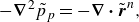 \begin{align} -\boldsymbol{\nabla} ^2 \tilde {p}_p & = -\boldsymbol{\nabla} \boldsymbol{\cdot} \tilde {\boldsymbol{r}}^{n}, \end{align}
 \begin{align} \frac {1}{2\,Re} D_2 \tilde {\boldsymbol{u}}_p - \left (\frac {1}{2\,Re} (\alpha ^2+\gamma ^2) + \frac {2}{Re\,\Delta t} \right ) \tilde {\boldsymbol{u}}_p - \boldsymbol{\nabla} \tilde {p}_p & = -\tilde {\boldsymbol{r}}^n, \end{align}
with $\tilde {p}_p(\pm h)=0$
and
$\tilde {p}_p(\pm h)=0$
and $\tilde {\boldsymbol{u}}_p(\pm h)=\boldsymbol{U}_b$
.
$\tilde {\boldsymbol{u}}_p(\pm h)=\boldsymbol{U}_b$
.
The components $\tilde {p}_t, \tilde {\boldsymbol{u}}_t$
solve
$\tilde {p}_t, \tilde {\boldsymbol{u}}_t$
solve
 \begin{align}&\qquad\qquad\qquad\qquad\quad -\boldsymbol{\nabla} ^2 \tilde {p}_t = 0, \end{align}
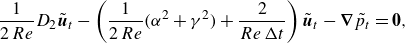 \begin{align}& \frac {1}{2\,Re} D_2 \tilde {\boldsymbol{u}}_t - \left (\frac {1}{2\,Re} (\alpha ^2+\gamma ^2) + \frac {2}{Re\,\Delta t} \right ) \tilde {\boldsymbol{u}}_t - \boldsymbol{\nabla} \tilde {p}_t = \boldsymbol{0}, \end{align}
with $\tilde {p}_t(h)=1,\ \tilde {p}_t(-h)=0$
and
$\tilde {p}_t(h)=1,\ \tilde {p}_t(-h)=0$
and $\tilde {\boldsymbol{u}}_t(\pm h)=\boldsymbol{0}$
.
$\tilde {\boldsymbol{u}}_t(\pm h)=\boldsymbol{0}$
.
The components $\tilde {p}_b, \tilde {\boldsymbol{u}}_b$
solve
$\tilde {p}_b, \tilde {\boldsymbol{u}}_b$
solve
 \begin{align}&\qquad\qquad\qquad\qquad\quad -\boldsymbol{\nabla} ^2 \tilde {p}_b = 0, \end{align}
 \begin{align}& \frac {1}{2\,Re} D_2 \tilde {\boldsymbol{u}}_b - \left (\frac {1}{2\,Re} (\alpha ^2+\gamma ^2) + \frac {2}{Re\,\Delta t} \right ) \tilde {\boldsymbol{u}}_b - \boldsymbol{\nabla} \tilde {p}_b = \boldsymbol{0}, \end{align}
with $\tilde {p}_b(h)=0,\ \tilde {p}_b(-h)=1$
and
$\tilde {p}_b(h)=0,\ \tilde {p}_b(-h)=1$
and $\tilde {\boldsymbol{u}}_b(\pm h)=\boldsymbol{0}$
.
$\tilde {\boldsymbol{u}}_b(\pm h)=\boldsymbol{0}$
.
The components $\tilde {p}_t^c, \tilde {\boldsymbol{u}}_t^c$
solve
$\tilde {p}_t^c, \tilde {\boldsymbol{u}}_t^c$
solve
 \begin{align}&\qquad\qquad\qquad\qquad -\boldsymbol{\nabla} ^2 \tilde {p}_t^c =-D_1 \sigma _t, \end{align}
 \begin{align}& \frac {1}{2\,Re} D_2 \tilde {\boldsymbol{u}}_t^c- \left (\frac {1}{2\,Re} (\alpha ^2+\gamma ^2) + \frac {2}{Re\,\Delta t} \right ) \tilde {\boldsymbol{u}}_t^c - \boldsymbol{\nabla} \tilde {p}^c_t = \boldsymbol{0}, \end{align}
with $\tilde {p}^c_t(\pm h)=0$
and
$\tilde {p}^c_t(\pm h)=0$
and $\tilde {\boldsymbol{u}}_t^c(\pm h)=\boldsymbol{0}$
. Note that
$\tilde {\boldsymbol{u}}_t^c(\pm h)=\boldsymbol{0}$
. Note that $\sigma _y$
has been further decomposed as
$\sigma _y$
has been further decomposed as $\sigma _y=\alpha _t^c \sigma _t + \alpha _b^c \sigma _b$
.
$\sigma _y=\alpha _t^c \sigma _t + \alpha _b^c \sigma _b$
.
Finally, the components $\tilde {p}_b^c,\tilde {\boldsymbol{u}}_b^c$
solve
$\tilde {p}_b^c,\tilde {\boldsymbol{u}}_b^c$
solve
 \begin{align}&\qquad\qquad\qquad\qquad -\boldsymbol{\nabla} ^2 \tilde {p}_b^c = -D_1 \sigma _b, \end{align}
 \begin{align}& \frac {1}{2\,Re} D_2 \tilde {\boldsymbol{u}}_b^c- \left (\frac {1}{2\,Re} (\alpha ^2+\gamma ^2) + \frac {2}{Re\,\Delta t} \right ) \tilde {\boldsymbol{u}}_b^c - \boldsymbol{\nabla} \tilde {p}^c_b = \boldsymbol{0}, \end{align}
with $\tilde {p}^c_b(\pm h)=0$
and
$\tilde {p}^c_b(\pm h)=0$
and $\tilde {\boldsymbol{u}}_b^c(\pm h)=0$
.
$\tilde {\boldsymbol{u}}_b^c(\pm h)=0$
.
After solving all the subsystems, one can assemble the solutions in (A5) to determine the four coefficients $\alpha _t, \alpha _b,\alpha _t^c, \alpha _b^c$
, requiring four equations. Two of the equations enforce the continuity equation at the boundaries, i.e.
$\alpha _t, \alpha _b,\alpha _t^c, \alpha _b^c$
, requiring four equations. Two of the equations enforce the continuity equation at the boundaries, i.e. $D_1 \tilde v^{n+1}=0$
at
$D_1 \tilde v^{n+1}=0$
at $y=\pm h$
or by substitution
$y=\pm h$
or by substitution
 \begin{align} D_1 \tilde v_p + \alpha _t D_1 \tilde v_t + \alpha _b D_1 \tilde v_b + \alpha ^c_t D_1 {\tilde v^c_t} + \alpha ^c_b D_1 {\tilde v^c_b} =&0 \quad \text{at} \ y=\pm h. \end{align}
The other two equations implement the boundary corrections, i.e.
 \begin{align}&\,\, \frac {1}{2\,Re} D_2{\tilde v^{n+1}} - \left (\frac {1}{2\,Re} (\alpha ^2+\gamma ^2) + \frac {2}{Re\,\Delta t} \right ) \tilde {v}^{n+1}- D_1 \tilde {p}^{n+1} = -\tilde r_y^n - \alpha ^c_t \quad \text{at} \ y=h, \end{align}
 \begin{align}& \frac {1}{2\,Re} D_2{\tilde v^{n+1}} - \left (\frac {1}{2\,Re} (\alpha ^2+\gamma ^2) + \frac {2}{Re\,\Delta t} \right ) \tilde {v}^{n+1} - D_1 \tilde {p}^{n+1}= -\tilde r_y^n - \alpha ^c_b \quad \text{at} \ y=-h. \end{align}
After these steps, we can obtain the pressure $\tilde {p}^{n+1}$
that enforces the continuity condition at all the grid points (including the boundary grid points), and
$\tilde {p}^{n+1}$
that enforces the continuity condition at all the grid points (including the boundary grid points), and $\tilde v^{n+1}$
at the next time step. The other two velocity components,
$\tilde v^{n+1}$
at the next time step. The other two velocity components, $\tilde u^{n+1}$
and
$\tilde u^{n+1}$
and $\tilde w^{n+1}$
, can be obtained by solving the Helmholtz equations (A3). When solving these equations, the matrix diagonalisation method proposed by Ehrenstein & Peyret (Reference Ehrenstein and Peyret1989) is employed, significantly enhancing the algorithm’s efficiency. To ensure accurate computation of the nonlinear terms in physical space, the
$\tilde w^{n+1}$
, can be obtained by solving the Helmholtz equations (A3). When solving these equations, the matrix diagonalisation method proposed by Ehrenstein & Peyret (Reference Ehrenstein and Peyret1989) is employed, significantly enhancing the algorithm’s efficiency. To ensure accurate computation of the nonlinear terms in physical space, the $3/2$
dealiasing rule is applied along the periodic directions.
$3/2$
dealiasing rule is applied along the periodic directions.
We present the validation of our numerical code in figure 10 for turbulent channel flow and turbulent Couette flow. For the channel flow with constant mass flux at $Re_\tau \approx 180$
, the computation domain is
$Re_\tau \approx 180$
, the computation domain is $(4\unicode{x03C0} , 2, {4}\unicode{x03C0}/{3})$
with resolution
$(4\unicode{x03C0} , 2, {4}\unicode{x03C0}/{3})$
with resolution $129\times 129\times 89$
, following the numerical set-up in Moser, Kim & Mansour (Reference Moser, Kim and Mansour1999). The length is normalised by the channel half-height. For the plane Couette flow, it is well known that the computational domain significantly influences flow statistics due to its impact on resolving large-scale dynamics (Komminaho, Lundbladh & Johansson Reference Komminaho, Lundbladh and Johansson1996; Pirozzoli, Bernardini & Orlandi Reference Pirozzoli, Bernardini and Orlandi2014). We chose to validate our implementation against the pseudo-spectral simulations of Lee & Kim (Reference Lee and Kim1991), following their numerical domain
$129\times 129\times 89$
, following the numerical set-up in Moser, Kim & Mansour (Reference Moser, Kim and Mansour1999). The length is normalised by the channel half-height. For the plane Couette flow, it is well known that the computational domain significantly influences flow statistics due to its impact on resolving large-scale dynamics (Komminaho, Lundbladh & Johansson Reference Komminaho, Lundbladh and Johansson1996; Pirozzoli, Bernardini & Orlandi Reference Pirozzoli, Bernardini and Orlandi2014). We chose to validate our implementation against the pseudo-spectral simulations of Lee & Kim (Reference Lee and Kim1991), following their numerical domain $(8\unicode{x03C0} /{3})$
and a similar resolution
$(8\unicode{x03C0} /{3})$
and a similar resolution $129\times 129\times 193$
along the
$129\times 129\times 193$
along the $x,y,z$
directions. As shown in the figure, our results exhibit good agreement with the classic data.
$x,y,z$
directions. As shown in the figure, our results exhibit good agreement with the classic data.
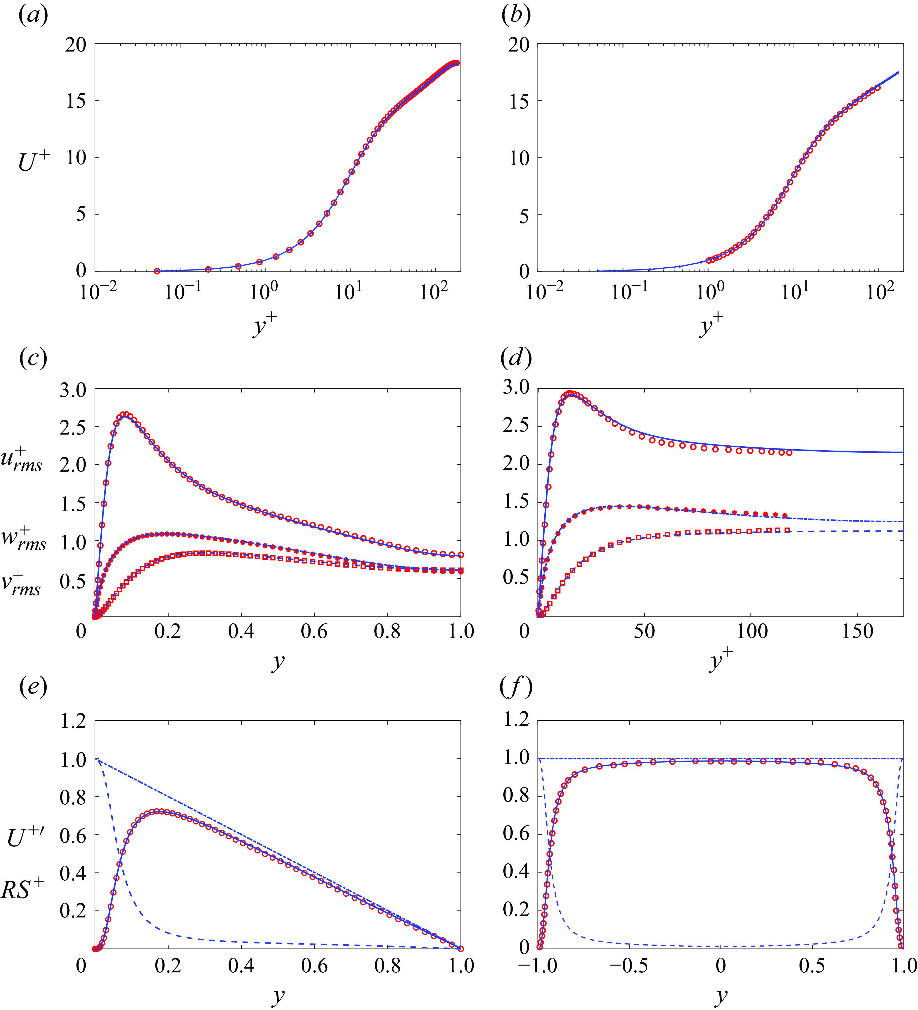
Figure 10. Verification of the DNS code: (a,b) mean velocity profiles; (c,d) profiles of turbulence intensities; (e,f) profiles of shear stresses. Solid lines indicate Reynolds stress ( $RS^+$
); dashed lines indicate viscous shear stress (
$RS^+$
); dashed lines indicate viscous shear stress ( ${U^+}'$
); dash-dotted lines indicate total stress). (a,c,e) Plane Poiseuille flow at
${U^+}'$
); dash-dotted lines indicate total stress). (a,c,e) Plane Poiseuille flow at $Re_\tau \approx 177.8$
compared to Moser et al. (Reference Moser, Kim and Mansour1999) (red symbols). (b,d,f) Plane Couette flow at
$Re_\tau \approx 177.8$
compared to Moser et al. (Reference Moser, Kim and Mansour1999) (red symbols). (b,d,f) Plane Couette flow at $Re_\tau \approx 171.8$
compared to Lee & Kim (Reference Lee and Kim1991) (red symbols), whose data points are extracted manually. Superscript
$Re_\tau \approx 171.8$
compared to Lee & Kim (Reference Lee and Kim1991) (red symbols), whose data points are extracted manually. Superscript $^+$
indicates normalisation with respect to the wall units. Here,
$^+$
indicates normalisation with respect to the wall units. Here, $y,y^+$
denote distance from a wall.
$y,y^+$
denote distance from a wall.


 Open access