


Impact Statement
The digital twin approach was originally developed to enhance decision-making for control by integrating measurement data. Its adoption in the construction industry, particularly in geotechnical engineering, has been hindered by difficulties associated with including uncertainties. While previous attempts to integrate uncertainties show promise, they are not fully compatible with geotechnical design and construction requirements. We propose a probabilistic DT framework that is specifically designed for geotechnical applications. Within this framework, major sources of uncertainty are integrated, including aleatoric, data, model, and prediction uncertainties, and they are propagated through the decision-making process. In an illustrative case study, this work explores the potential of the PDT to leverage existing probabilistic methods PDT for integrating measurement data and improving decision-making in geotechnical design and construction. By embedding these methods within a structured framework, the PDT facilitates their practical adoption, overcoming existing implementation challenges and making probabilistic approaches more accessible to engineering practitioners.
1. Introduction
The digital twin (DT) concept, introduced by Grieves (Reference Grieves2002), emerged in response to a changing reality, where the amount of data collected across all industries vastly increased due to technological advancements. Digital methods are required for real-time data processing and decision-making to leverage this for productivity gains. Thus, the DT shows potential for addressing challenges confronting the Architecture, Engineering, Construction, Operations, and Management (AECOM) industries. These challenges include managing the increasing flow of project-related data, low productivity, unpredictability in terms of costs and schedules, and complexity attributed to structural fragmentation (Opoku et al., Reference Opoku, Perera, Osei-Kyei and Rashidi2021).
While the DT concept has been adopted to address these challenges in some areas of AECOM, e.g., for facility management with the control of heating, ventilation, and air conditioning (Xie et al., Reference Xie, Merino, Moretti, Pauwels, Chang and Parlikad2023), its broader application remains limited. One significant obstacle is that projects in these industries are characterized by significant uncertainties resulting from the unique and complex nature of projects. These uncertainties are particularly large in the geotechnical phase of construction projects due to the inherent variability of soil and the limited availability of observational data (Phoon et al., Reference Phoon, Cao, Ji, Leung, Najjar, Shuku, Tang, Yin, Ikumasa and Ching2022a).
Traditional DT approaches rely on deterministic input parameters and models to predict the behavior of the physical twin. The accuracy of the traditional DT depends on having complete knowledge of the physical asset, which is usually unattainable. Uncertainties arising from a lack of knowledge cannot be incorporated. Instead, uncertainties are reduced to deterministic values, resulting in a loss of valuable information when decisions are made. For example, in practice, it is common to consider worst-case scenarios and then account for uncertainties by applying safety factors. This can lead to over-conservative designs that are too safe and thus inefficient in terms of resource use. In other cases, when extrapolation from so-called worst-case scenarios is needed, designs may be unsafe. Thus, a deterministic DT lacks the capability of accurate predictions in the presence of significant uncertainty.
In recent years, there have been proposals to extend traditional DTs with uncertainty analysis, which leverages the capabilities of Bayesian methods for integrating additional data. Knowledge from previous projects or domain expertise is incorporated as prior belief states, which can be updated as additional information is obtained. Previous approaches can be found under various names such as predictive digital twin (Kapteyn et al., Reference Kapteyn, Pretorius and Willcox2021; Chaudhuri et al., Reference Chaudhuri, Pash, Hormuth, Lorenzo, Kapteyn, Wu, Lima, Yankeelov and Willcox2023; Torzoni et al., Reference Torzoni, Tezzele, Mariani, Manzoni and Willcox2024), probabilistic digital twin (Nath and Mahadevan, Reference Nath and Mahadevan2022; Agrell et al., Reference Agrell, Rognlien Dahl and Hafver2023) or DT concepts with uncertainty (Kochunas and Huan, Reference Kochunas and Huan2021). However, they are not tailored to the specific requirements of geotechnical construction, as we detail in Section 2.2. Phoon et al. (Reference Phoon, Ching and Cao2022b) show that in order for the geotechnical engineering field to benefit from emerging digital technologies, these must be tailored to the unique characteristics of the field, where data is sparse, incomplete, of low quality, and originates from multiple sources.
The objective of this work is to develop a PDT framework that can be used for geotechnical design and construction. Specifically, we show that for a framework to be scalable and applicable across all project stages, data should be classified into two types—property and behavioral data—which are relevant at different modeling stages. The effectiveness of the PDT framework is shown through an application to a highway foundation construction project, demonstrating its potential to improve decision-making and project outcomes in the face of uncertainties. After the PDT is created, the optimization of this decision-making process is compared with state-of-the-art optimization based on Monte Carlo Simulation. While probabilistic methods for decision-making already exist, they are rarely applied in practice due to implementation barriers. The PDT framework addresses this gap by facilitating their integration into engineering workflows.
The remainder of the paper is organized as follows. Section 2 contains reviews of existing PDT approaches and proposes a modified PDT framework to address the needs of AECOM systems and projects. The mathematical formulation of this framework follows in Section 3. In Section 4, the specifics of each PDT component are discussed in the context of geotechnical design and construction. Section 5 describes an analysis of the benefits, potential, and challenges of implementing a PDT approach, illustrated through a numerical investigation and the results in Section 5.4. This is followed by a discussion in Section 6 and conclusions in Section 7.
2. PDT concept
2.1. Traditional digital twins
As industries began adopting the DT concept over the last two decades, there followed a series of definitions and interpretations (Brilakis et al., Reference Brilakis, Pan, Borrmann, Mayer, Rhein, Vos, Pettinato and Wagner2019). In the literature, review articles are available that examine definitions, current approaches, challenges, and opportunities across several industries (e.g., Liu et al., Reference Liu, Fang, Dong and Xu2021; Opoku et al., Reference Opoku, Perera, Osei-Kyei and Rashidi2021; Semeraro et al., Reference Semeraro, Lezoche, Panetto and Dassisti2021; Singh et al., Reference Singh, Srivastava, Fuenmayor, Kuts, Qiao, Murray and Devine2022; Li et al., Reference Li, Rui, Zhao, Zhang and Zhu2024; Babanagar et al., Reference Babanagar, Sheil, Ninić, Zhang and Hardy2025). Most definitions share three fundamental components of a DT: the physical object, the digital replica, and the bidirectional communication between the two. Kritzinger et al. (Reference Kritzinger, Karner, Traar, Henjes and Sihn2018) state that, compared to other digital representations, DTs place a specific emphasis on the dual identification-control aspect. Accordingly, we adopt the definition of Kritzinger et al. (Reference Kritzinger, Karner, Traar, Henjes and Sihn2018), where digital representations of physical entities are categorized into three categories: (a) the Digital Model, which does not involve automated data exchange between the physical and digital object. Any state change in the physical has to be manually implemented inside the digital object; (b) the Digital Shadow, with a one-way automated data flow from the physical to the digital object, enabling automated monitoring of the physical state; (c) the DT, which includes automated information exchange in both directions and is capable of accurately mirroring the state of the physical entity. The insights gained from modeling and predicting the behavior of the physical entity can be leveraged for operational decision-making.
Alternatively, Li et al. (Reference Li, Rui, Zhao, Zhang and Zhu2024) propose a four-level maturity framework for DTs based on their capabilities: description twin, reflective twin, prediction twin, and prescriptive twin. The DT definition proposed by Kritzinger et al. (Reference Kritzinger, Karner, Traar, Henjes and Sihn2018) aligns with a prescriptive twin, in which predicted behavior is used to optimize control commands. This differentiates it from a prediction twin, which only forecasts behavior without optimizing control. Digital shadows (Kritzinger et al., Reference Kritzinger, Karner, Traar, Henjes and Sihn2018) correspond to reflective twins and are digital representations that reflect the current known state of the physical asset. The digital model is equivalent to a description twin, a digital representation that lacks updating and predictive capabilities. These maturity frameworks provide structured approaches for evaluating DT implementations (Babanagar et al., Reference Babanagar, Sheil, Ninić, Zhang and Hardy2025).
2.2. Prior work in PDTs
Kapteyn et al. (Reference Kapteyn, Pretorius and Willcox2021) were among the first to formalize a probabilistic approach to DTs, particularly for unmanned aerial vehicles. In their work, the DT is modeled as a probabilistic graphical model, using Bayesian methods for model updating and decision-making. This framework is scalable and can be extended to applications across multiple industries. For example, Chaudhuri et al. (Reference Chaudhuri, Pash, Hormuth, Lorenzo, Kapteyn, Wu, Lima, Yankeelov and Willcox2023) adapted this framework to the needs of risk-aware clinical decision-making, facilitating anticipatory, personalized tumor treatment that accounts for uncertainty. Torzoni et al. (Reference Torzoni, Tezzele, Mariani, Manzoni and Willcox2024) extended the approach to structural health monitoring and management of civil engineering structures. They highlight the potential for assimilating structural response data using deep learning methods, enabling a change towards data-driven, predictive maintenance practices of bridges. However, these approaches primarily focus on behavioral aspects of systems, where physical states are observed indirectly through structural response measurements. We refer to this type of data as behavior data. This data type is distinguished from property data, which consists of direct measurements of the properties of the physical twin. This classification is detailed in Section 2.3.3. In many industries, property data carries low uncertainties, but in the construction industry—and particularly in geotechnical engineering—they are associated with large uncertainty. For example, borehole soundings are used to determine soil types and properties at the measurement locations. However, due to typically sparse measurements and the inherent variability of soils, significant uncertainties arise when extrapolating to unmeasured locations. A comprehensive PDT designed to support the full process of geotechnical design and construction must therefore differentiate between behavior and property data.
Kochunas and Huan (Reference Kochunas and Huan2021) demonstrated the potential of quantifying uncertainties in the DT approach for nuclear power systems, with a focus on understanding the sources of uncertainty in the modeling process and their propagation throughout the entire lifecycle. Nath and Mahadevan (Reference Nath and Mahadevan2022) introduced the PDT concept for additive manufacturing, specifically for the laser powder bed fusion process. By incorporating measurement and model uncertainties, this approach enables early-stage design optimization and predictive maintenance. Alibrandi (Reference Alibrandi2022) introduced the concept of a risk-informed DT to support sustainable and resilient engineering for urban communities. Agrell et al. (Reference Agrell, Rognlien Dahl and Hafver2023) provided a formal mathematical definition of a PDT and highlighted its potential for sequential decision-making under uncertainties. Despite these advancements, these approaches to PDTs are often tailored to specific applications, making their application to geotechnical design and construction unclear. They typically focus on a single phase of the PDT—design, construction, or operation—rather than addressing the entire lifecycle. As a result, their general applicability is limited, with each specific application requiring a customized PDT. This fragmented approach diminishes the potential benefits of integrating data and predictive behavior models into a unified framework.
To achieve a successful implementation of a PDT in geotechnical design and construction, the framework should ideally include several key components: (1) the creation of (3D) subsoil models from sparse property data (e.g., borehole soundings), (2) behavioral prediction of quantities of interest (e.g., settlement under load), (3) integration of established modeling methods to ensure trust, (4) initialization of historical data and expert knowledge at initial stages, (5) model updating for additional information, and (6) optimization of sequential decision-making under uncertainty.
In this work, we introduce a PDT framework that encompasses these key components. Like previous approaches, it extends the traditional DT to incorporate uncertainty quantification, enabling the use of Bayesian methods for data integration. However, it extends previous approaches, as it is specifically designed for scalability and differentiates between the two types of data. The PDT is demonstrated through a case study involving a highway foundation construction project, but it has broad applicability within AECOM industries. To the best of our knowledge, this research represents the PDT concept in the context of geotechnical design and construction.
2.3. PDT framework
In Figure 1, the PDT framework is summarized. This framework encapsulates the physical state, representing the physical system and its interactions with the environment, from which data on properties and behaviors are obtained. In cases where data is used directly for decision-making, the entire modeling step can be skipped (see dashed line). However, this is rarely the case in civil engineering, where data is sparse, systems are complex, and explainability for decisions is required. In such cases, in the learning process, through statistical and mathematical modeling, property data is transformed into the digital state. This state captures all necessary attributes to model the physical state and is utilized in modeling the behavioral prediction, which mirrors the behavior of the physical twin to predict future states. Behavior data is used to update and calibrate the parameters of the behavioral prediction models, as well as the digital state. These predictions support decision optimization, aiming to identify optimal decisions regarding controlling actions, which alter the physical state, and decisions to collect additional information to reduce model uncertainties.
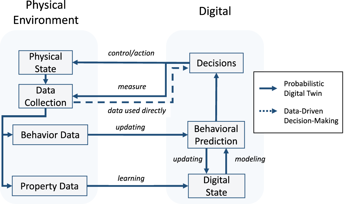
Figure 1. Schematic flowchart of the proposed PDT framework, where dashed arrows represent the data-driven decision path, while solid arrows highlight the path of the proposed PDT.
In the following subsections, each component and process is discussed within the scope of construction engineering. We illustrate how each component relates to components of the traditional DT approach and how they are extended to accommodate uncertainties.
2.3.1. Physical state
The physical state includes both the physical twin, which is the object of the PDT modeling process, its interactions with the surrounding environment, and the data acquisition technologies that enable the collection of system state information. Recent advancements in these technologies have significantly increased the volume of collected data, necessitating specialized tools to enhance the decision-making process.
2.3.2. Digital state
Since the primary objective of the PDT is to enhance decision-making for a specific use case, the modeling process must begin with a detailed requirements analysis. This analysis aims to identify the key quantities of interest and the necessary information requirements based on the defined use cases. By modeling and predicting the behavior of these quantities, decision-making can be improved. The process involves selecting appropriate models and determining the necessary input data. Predictions must be validated against measured behavioral data for calibration. Such a requirement analysis is a complex task that necessitates extensive domain expertise, comprehensive knowledge of applicable methodologies, and the necessary level of detail for each project phase. As a rule, simple models generally suffice for initial phases, whereas more detailed models are necessary for later stages. This model progression approach is comparable to the level of detail (LoD) used in disciplines like computer graphics and recognized in the AECOM industries under various terminologies (Abualdenien and Borrmann, Reference Abualdenien and Borrmann2022). First applications of this in geotechnical design are introduced by Ninić et al. (Reference Ninić, Koch and Stascheit2017); Huang et al. (Reference Huang, Zhu, Ninić and Zhang2022) where the LoD concept is considered for underground tunnelling and metro construction, respectively. The PDT could leverage this concept to quantify model uncertainties correlated to the level of model detail.
At the beginning of the modeling process, a detailed requirements analysis should identify the quantities of interest, which are the critical parameters of the physical twin that should drive the decision optimization process. To predict the evolution of quantities of interest over time, appropriate models and their input parameters are required.
Essential questions that should be addressed in the requirement analysis include: What is the object of the modeling effort? What are the quantities of interest, quantities of the physical twin? Which models are appropriate for this purpose? What properties are essential for these models to function effectively? What methods are available to acquire the necessary observations? What actions are possible to change the state of the physical twin? By what operational constraints are they affected? Among others, these questions form a robust foundation for a modeling strategy and result in a set of parameters that contain all important aspects of the physical twin, thereby enhancing the accuracy and utility of the PDT. A distinctive feature of the PDT approach is its ability to represent these parameters both deterministically and stochastically, allowing it to incorporate the inherent uncertainties and unknowns within complex systems.
2.3.3. Data
Data can be categorized into two classes:
(1) Property data are direct observations of the attributes or properties of the physical twin (e.g., shear strength of soils or concrete). They are used to learn the parameters included in the digital state. The observations are obtained through intrusive methods (e.g., field tests, compressive strength tests, fatigue testing) or non-intrusive methods (e.g., geophysical, visual inspection of concrete, tomographic modeling). Sparse data availability is common due to the damaging nature of excessive intrusive testing and the high costs of performing experiments.
(2) Behavior data is obtained by monitoring the behavior of the PT over time (e.g., soil settlement, building temperature, crack propagation in concrete). They do not provide direct insights into the state and attributes of the physical twin. Instead, they contain the monitored behavior over time and are used to calibrate predictive models and reduce their uncertainty.
Both classes of data are subject to observation uncertainty, which can be caused by limited measurement precision, faulty calibration of measurement devices, misreporting, among other reasons. This uncertainty is quantified by likelihood functions (Agrell et al., Reference Agrell, Rognlien Dahl and Hafver2023) and is typically an order of magnitude smaller than other modeling uncertainties.
2.3.4. Learning the digital state
To learn the digital state from property data, commonly two steps are performed:
(1) Where properties of interest cannot be measured directly, transformation models are required to obtain them from property data. For example, in geotechnical engineering, empirical transformation models are used to categorize soil types (e.g., clay, sand, silt) based on mechanical properties derived from cone penetration test soundings (Robertson, Reference Robertson2009). In this step, uncertainties introduced due to the assumptions of the transformation model have to be accounted for (e.g., Wang C.H. et al., Reference Wang, Harken, Osorio-Murillo, Zhu and Rubin2016; Wang X. et al., Reference Wang, Wang, Liang, Zhu and Di2018; Wang H. et al., Reference Wang, Wang, Wellmann and Liang2019).
(2) Inference of properties at unobserved locations is required due to the spatial variability of soil properties and the sparsity of data. In geotechnical engineering, Kriging interpolation, or Gaussian Process Regression (GPR), is commonly applied to simulate subsoil models (e.g., Gong et al., Reference Gong, Zhao, Juang, Tang, Wang and Hu2020; Yoshida et al., Reference Yoshida, Tomizawa and Otake2021). This probabilistic approach can quantify uncertainties introduced during modeling, which depend on the underlying assumptions and the quality and quantity of available data (Rasmussen and Williams, Reference Rasmussen and Williams2005).
The traditional DT approach is not capable of incorporating these uncertainties. Therefore, even when stochastic methods like GPR are used, the resulting uncertainties are frequently discarded, and only the expected values are utilized for predictions. In comparison, the PDT approach actively incorporates and propagates uncertainties through all modeling stages to enhance model robustness. By integrating stochastic learning methods, sparse data can be supplemented with information from similar regional projects or expert domain knowledge.
2.3.5. Behavioral prediction modeling and updating
The predictive models within the DT framework aim to accurately simulate the behavior of their physical counterparts (Chaudhuri et al., Reference Chaudhuri, Pash, Hormuth, Lorenzo, Kapteyn, Wu, Lima, Yankeelov and Willcox2023). Such models establish relationships between measurable physical attributes and the behavior of the physical twin (Agrell et al., Reference Agrell, Rognlien Dahl and Hafver2023). By capturing these relationships, the models predict quantities of interest that inform subsequent decision optimization processes.
Traditionally, behavioral prediction models have been categorized into two main categories: physics-based models (e.g., finite element methods), which rely on an explicit representation of the physics of the system, and data-driven models (e.g., regression models, machine learning), where observation are directly interpreted to learn patterns and correlations. To overcome the limitations of each type, hybrid models were developed (e.g., physics-informed machine learning Karniadakis et al. (Reference Karniadakis, Kevrekidis, Lu, Perdikaris, Wang and Yang2021)). They combine the interpretability and accuracy of physics-based models with the computational efficiency of data-driven models. Additionally, surrogate models are approximations of complex models designed to capture their essential features. Examples include artificial neural networks (Zhang et al., Reference Zhang, Li, Li, Liu, Chen and Ding2021), Gaussian Process models (Gramacy, Reference Gramacy2020), or polynomial chaos expansion (Sudret, Reference Sudret2014). The PDT uses Bayesian inference to update prediction models as new information becomes available. Bayesian inference is a statistical method that combines prior probability distributions with measurement likelihoods to estimate a posterior distribution. This approach can be used within the PDT framework since uncertain parameters are represented as random variables.
Throughout the life cycle of the physical twin, multiple quantities of interest must be predicted based on phase-specific requirements and objectives. The PDT facilitates the integration of multiple probabilistic models and methods into a centralized platform, enabling efficient data sharing and model selection. When faced with a prediction task, the most suitable model is chosen from a set of available models, allowing for adaptability across different scenarios. This is particularly crucial for systems vulnerable to extreme events (e.g., earthquakes, floods, storms), where sudden changes in conditions can significantly affect predictions. Selecting the appropriate model for each scenario is a critical engineering decision that requires careful evaluation and expertise.
From a practical perspective, integrating multiple behavioral prediction models is particularly challenging in civil and geotechnical engineering, where specialized software is required for specific tasks. For example, commonly used finite element analysis software in geotechnical engineering (e.g., Plaxis 2D/3D and Geostudio) could be integrated into the PDT via their APIs. However, each software solution has unique input requirements and produces distinct outputs, requiring customized integration.
Despite these challenges, integrating multiple models within the PDT offers significant advantages, as it can contribute to overcoming silos and provides the ability to propagate knowledge and uncertainties throughout the modeling process.
2.3.6. Decision making
-
a) Levels of automation: Decision-making in AECOM industries is particularly challenging due to the societal impact and size of projects. In addition, personally liable, and decisions at every step have to be well-founded and explainable. The goal of the PDT framework is to actively manage uncertainties and provide support for decision-making in near-real-time. However, before achieving effective support for decision-making, trust must be established, and the accuracy of the used models should be assured. Explainability of decisions is a crucial factor. For this reason, we envision a two-level adoption of the PDT approach:
-
(1) Semi-automated level: In this stage, a hybrid human-computer decision-making approach is employed. The objective is to build trust and improve decision-making to a level replicating at least the accuracy of human counterparts. At this stage, the PDT serves as a supportive platform, offering decision recommendations to engineers who then choose how to proceed.
-
(2) Intelligent support for decision-making: Achieving intelligent support for decision-making in the AECOM industry necessitates not only improved accuracy and increased trust but also significant technological advancements. When technological breakthroughs increase the degree of automation on site, the PDT framework is designed to automate and optimize support for the decision-making process. For example, in the future, automated, driver-free excavators could rely on the PDT to decide where and how much to dig. Simultaneously, the data collected by the sensors of the excavator could be used to update the digital state so that the system learns from its experience. Applications of automated control in geotechnical engineering can already be found in underground construction, where the operating parameters of tunneling machines are automatically adjusted based on soil conditions and the potential impact on surrounding buildings (e.g., Freitag et al., Reference Freitag, Cao, Ninić and Meschke2018; Zhang et al., Reference Zhang, Chen and Wu2019; Reference Zhang, Guo, Fu, Tiong and Zhang2024; Liu et al., Reference Liu, Li and Liu2022).
-
-
(b) Types of decisions: Engineering decisions typically fall into two categories (Benjamin and Cornell, Reference Benjamin and Cornell2014):
-
(1) Information collection (
 $ e $
) to reduce epistemic uncertainties and improve model predictions. These decisions involve determining the optimal timing and location for data acquisition, considering both costs and potential information gain.
$ e $
) to reduce epistemic uncertainties and improve model predictions. These decisions involve determining the optimal timing and location for data acquisition, considering both costs and potential information gain. -
(2) Control actions (
$ a $
) aimed at improving system design or performance by simulating various scenarios and evaluating decision outcomes. Applications in geotechnical engineering include optimizing engineering designs, such as improving the design of road embankments (Bismut et al., Reference Bismut, Cotoarbă, Spross and Straub2023), assessing risks in foundation pit excavations (Sun et al., Reference Sun, Li, Bao, Meng and Zhang2023), and automated control of tunneling machines (Ninić and Meschke Reference Ninić and Meschke2015; Freitag et al., Reference Freitag, Cao, Ninić and Meschke2018; Zhang et al., Reference Zhang, Chen and Wu2019, Reference Zhang, Guo, Fu, Tiong and Zhang2024; Liu et al., Reference Liu, Li and Liu2022; Roper et al., Reference Roper, Bertuzzi, Oliveira and Karlovšek2024).
-


Good decision-making relies on behavioral prediction models to analyze various scenarios and assess the potential impact of decisions on quantities of interest. The output of the evaluation is a decision metric used to objectively compare decisions, called a reward. In the context of AECOM, potential rewards include reliability, cost, or environmental impact. Incorporating uncertainties in the PDT increases the computational demands, especially when decisions must account for both present and future state uncertainties. Optimization methods include Partially Observable Markov Decision Process (POMDP) solvers, Reinforcement Learning, and Heuristic Strategy Optimization (Porta et al., Reference Porta, Spaan and Vlassis2005; Roy et al., Reference Roy, Gordon and Thrun2005; Silver and Veness, Reference Silver and Veness2010; Papakonstantinou et al., Reference Papakonstantinou, Andriotis and Shinozuka2018; Andriotis and Papakonstantinou, Reference Andriotis and Papakonstantinou2019; Bismut and Straub, Reference Bismut and Straub2021).
3. Mathematical model of the PDT
An influence diagram is utilized to model the PDT, shown in Figure 2. Introduced by Shachter (Reference Shachter1986), influence diagrams serve as a graphical tool to represent decision-making scenarios under uncertainty (Jensen and Nielsen, Reference Jensen and Nielsen2007; Koller and Friedman, Reference Koller and Friedman2009). Influence diagrams are acyclic-directed graphs in which round nodes represent random variables (RV), squared nodes represent decisions, and rhombus nodes represent utility functions. Directed arrows connect the nodes and specify the dependence structure among the RVs.
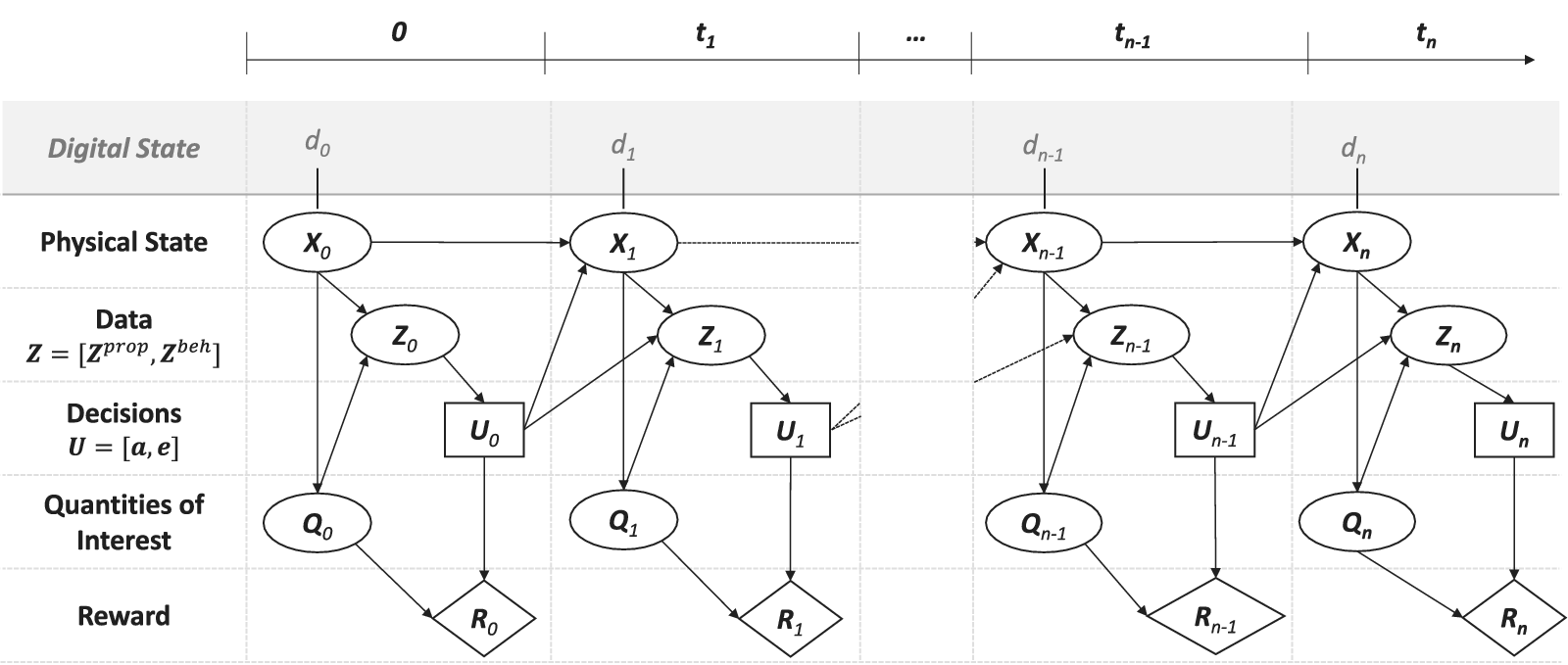
Figure 2. The proposed PDT model is represented by an influence diagram to highlight the conditional dependencies of the individual components.
The PDT model incorporates the Markov assumption, which implies that the current state—if known—summarizes all the information contained in past states and data (Norris, Reference Norris1998). This allows for a simplified mathematical representation of belief states and their conditional dependencies across time. For applications where the Markov assumption does not hold a-priori, the model is still applicable through state space augmentation (Kitagawa, Reference Kitagawa1998).
The PDT model describes the relation between the physical state
 $ {\mathbf{X}}_t $
, the data
$ {\mathbf{X}}_t $
, the data
 $ \mathbf{Z} $
, which includes the property data
$ \mathbf{Z} $
, which includes the property data
 $ {\boldsymbol{Z}}^{\mathrm{prop}} $
and the behavioral data
$ {\boldsymbol{Z}}^{\mathrm{prop}} $
and the behavioral data
 $ {\boldsymbol{Z}}^{\mathrm{beh}} $
, the quantities of interest
$ {\boldsymbol{Z}}^{\mathrm{beh}} $
, the quantities of interest
 $ {\mathbf{Q}}_t $
, the decisions
$ {\mathbf{Q}}_t $
, the decisions
 $ \mathbf{U} $
and the rewards
$ \mathbf{U} $
and the rewards
 $ {\mathbf{R}}_t $
. As discussed in Section 2.3.6, the decisions are of two types
$ {\mathbf{R}}_t $
. As discussed in Section 2.3.6, the decisions are of two types
 $ \mathbf{U}=\left[\mathbf{e},\mathbf{a}\right] $
. The quantities of interest are the result of the behavioral prediction.
$ \mathbf{U}=\left[\mathbf{e},\mathbf{a}\right] $
. The quantities of interest are the result of the behavioral prediction.
The state
 $ {\mathbf{X}}_t $
state is generally unknown and only represented probabilistically; it corresponds to the hidden state in a hidden Markov model (Koller and Friedman, Reference Koller and Friedman2009). Therefore, what is known about
$ {\mathbf{X}}_t $
state is generally unknown and only represented probabilistically; it corresponds to the hidden state in a hidden Markov model (Koller and Friedman, Reference Koller and Friedman2009). Therefore, what is known about
 $ {\mathbf{X}}_t $
is its (posterior) distribution. In the sequential decision-making under uncertainty literature, this distribution over the state is known as the belief (Kochenderfer, Reference Kochenderfer2015). This belief is what we refer to as the digital state
$ {\mathbf{X}}_t $
is its (posterior) distribution. In the sequential decision-making under uncertainty literature, this distribution over the state is known as the belief (Kochenderfer, Reference Kochenderfer2015). This belief is what we refer to as the digital state
 $ {d}_t $
in this framework.
$ {d}_t $
in this framework.
The digital state
 $ {d}_t=p\left({\mathbf{X}}_t|{\mathbf{Z}}_{0:t}={\mathbf{z}}_{0:t},{\mathbf{U}}_{0:t-1}={\mathbf{u}}_{0:t-1}\right) $
is the distribution of
$ {d}_t=p\left({\mathbf{X}}_t|{\mathbf{Z}}_{0:t}={\mathbf{z}}_{0:t},{\mathbf{U}}_{0:t-1}={\mathbf{u}}_{0:t-1}\right) $
is the distribution of
 $ {\mathbf{X}}_t $
conditional on all past and current observations
$ {\mathbf{X}}_t $
conditional on all past and current observations
 $ {\mathbf{z}}_{0:t} $
and all past decisions
$ {\mathbf{z}}_{0:t} $
and all past decisions
 $ {\mathbf{u}}_{0:t-1} $
. It represents the knowledge of the physical state
$ {\mathbf{u}}_{0:t-1} $
. It represents the knowledge of the physical state
 $ {\mathbf{X}}_t $
within the PDT. The digital state evolves dynamically as new data is obtained and decisions are made. Its transition dynamics and update with new data
$ {\mathbf{X}}_t $
within the PDT. The digital state evolves dynamically as new data is obtained and decisions are made. Its transition dynamics and update with new data
 $ \mathbf{Z} $
are given by
$ \mathbf{Z} $
are given by
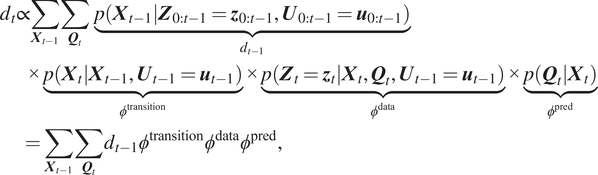 $$ {\displaystyle \begin{array}{l}{d}_t\propto \sum_{{\boldsymbol{X}}_{t-1}}\sum_{{\boldsymbol{Q}}_t}\hskip0.35em \underset{d_{t-1}}{\underbrace{p\left({\boldsymbol{X}}_{t-1}|{\boldsymbol{Z}}_{0:t-1}={\boldsymbol{z}}_{0:t-1},{\boldsymbol{U}}_{0:t-1}={\boldsymbol{u}}_{0:t-1}\right)}}\\ {}\hskip2em \times \underset{\phi^{\mathrm{transition}}}{\underbrace{p\left({\boldsymbol{X}}_t|{\boldsymbol{X}}_{t-1},{\boldsymbol{U}}_{t-1}={\boldsymbol{u}}_{t-1}\right)}}\times \underset{\phi^{\mathrm{data}}}{\underbrace{p\left({\boldsymbol{Z}}_t={\boldsymbol{z}}_t|{\boldsymbol{X}}_t,{\boldsymbol{Q}}_t,{\boldsymbol{U}}_{t-1}={\boldsymbol{u}}_{t-1}\right)}}\times \underset{\phi^{\mathrm{pred}}}{\underbrace{p\left({\boldsymbol{Q}}_t|{\boldsymbol{X}}_t\right)}}\\ {}\hskip2em =\sum_{{\boldsymbol{X}}_{t-1}}\sum_{{\boldsymbol{Q}}_t}{d}_{t-1}{\phi}^{\mathrm{transition}}{\phi}^{\mathrm{data}}{\phi}^{\mathrm{pred}},\end{array}} $$
and has the following four components:
-
1.
$ {d}_{t-1}=p\left({\mathbf{X}}_{t-1}|{\mathbf{Z}}_{0:t-1}={\mathbf{z}}_{0:t-1},{\mathbf{U}}_{0:t-1}={\mathbf{u}}_{0:t-1}\right) $
is the digital state at the previous time step. It encapsulates the cumulative history up to time
$ t-1 $
. It is obtained by recursively applying Equation (1), with an initial prior at
$ t=0 $
that incorporates any pre-existing knowledge and expertise, as well as initial property data, following Section 2.3.4. -
2.
$ {\varphi}^{\mathrm{transition}}=p\left({\boldsymbol{X}}_t|{\boldsymbol{X}}_{t-1},{\boldsymbol{U}}_{t-1}={\boldsymbol{u}}_{t-1}\right) $
is the state transition from
$ {\mathbf{X}}_{t-1} $
to
$ {\mathbf{X}}_t $
influenced by the controlling actions
$ {\mathbf{a}}_{t-1} $
. -
3.
$ {\varphi}^{\mathrm{data}}=p\left({\boldsymbol{Z}}_t={\boldsymbol{z}}_t|{\boldsymbol{X}}_t,{\boldsymbol{Q}}_t,{\boldsymbol{U}}_{t-1}={\boldsymbol{u}}_{t-1}\right) $
is the likelihood of describing the data. It is conditional on
$ {\mathbf{e}}_{t-1} $
, the decision on what data should be collected. Given the distinction between the two types of data, this component can be divided into two parts:


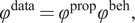 $$ {\varphi}^{\mathrm{data}}={\varphi}^{\mathrm{prop}}{\varphi}^{\mathrm{beh}}, $$
with
 $ {\varphi}^{\mathrm{prop}}=p\left({\boldsymbol{z}}_t^{\mathrm{prop}}|{\boldsymbol{X}}_t,{\boldsymbol{U}}_{t-1}={\boldsymbol{u}}_{t-1}\right) $
being the likelihood of the property data and
$ {\varphi}^{\mathrm{prop}}=p\left({\boldsymbol{z}}_t^{\mathrm{prop}}|{\boldsymbol{X}}_t,{\boldsymbol{U}}_{t-1}={\boldsymbol{u}}_{t-1}\right) $
being the likelihood of the property data and
 $ {\varphi}^{\mathrm{beh}}=p\left({\boldsymbol{z}}_t^{\mathrm{beh}}|{\boldsymbol{Q}}_t,{\boldsymbol{U}}_{t-1}={\boldsymbol{u}}_{t-1}\right) $
the likelihood of the behavior data.
$ {\varphi}^{\mathrm{beh}}=p\left({\boldsymbol{z}}_t^{\mathrm{beh}}|{\boldsymbol{Q}}_t,{\boldsymbol{U}}_{t-1}={\boldsymbol{u}}_{t-1}\right) $
the likelihood of the behavior data.
-
4.
$ {\varphi}^{\mathrm{pred}}=p\left({\boldsymbol{Q}}_t|{\boldsymbol{X}}_t\right) $
describes the dependency of the quantity of interest
$ {\mathbf{Q}}_t $
on the state
$ {\mathbf{X}}_t $
.


The evolution and updating of the digital state according to Equation (1) results from the rules for probabilistic graphical models (Koller and Friedman, Reference Koller and Friedman2009). Figure 3 is a graphical representation of this process, highlighting the opposite flow of information in the updating process compared to the causal dependencies of the underlying graphical model.
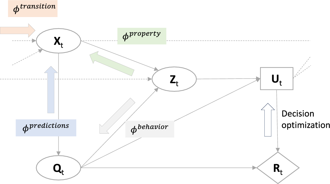
Figure 3. Illustration of the transition and updating with new data
 $ {z}_t=\left[{z}_t^{\mathrm{prop}},{z}_t^{\mathrm{beh}}\right] $
in one time step of the PDT.
$ {z}_t=\left[{z}_t^{\mathrm{prop}},{z}_t^{\mathrm{beh}}\right] $
in one time step of the PDT.
While Equation (1) implies that the physical state and the quantity of interest are discrete random variables, the PDT formulation is general. Continuous random variables can be included by replacing the summations in the equation with integrals. However, in practice, solutions with straightforward numerical integration are not possible for high-dimensional problems. In such cases, sampling approaches can be used to create an approximation of
 $ {\mathbf{X}}_t $
(Russell and Norvig, Reference Russell and Norvig2016).
$ {\mathbf{X}}_t $
(Russell and Norvig, Reference Russell and Norvig2016).
One such approach is the particle filter (PF) approach Doucet et al. (Reference Doucet, De Freitas and Gordon2001), (Reference Doucet and Johansen2009), which is simple and has the ability to perform online updating (Kamariotis et al., Reference Kamariotis, Sardi, Papaioannou, Chatzi and Straub2023). It is a sequential importance sampling technique for approximating the posterior with weighted samples.
The basic PF begins at
 $ t=0 $
by generating samples of
$ t=0 $
by generating samples of
 $ {\mathbf{X}}_0 $
from the initial digital state (the prior distribution of
$ {\mathbf{X}}_0 $
from the initial digital state (the prior distribution of
 $ {\mathbf{X}}_0 $
). These samples are subsequently updated based on behavior data (settlement measurements) and actions (surcharge adjustments). At each time step, the Bayesian update is performed by evaluating
$ {\mathbf{X}}_0 $
). These samples are subsequently updated based on behavior data (settlement measurements) and actions (surcharge adjustments). At each time step, the Bayesian update is performed by evaluating
 $ {\varphi}_k^{\mathrm{beh}} $
for every sample
$ {\varphi}_k^{\mathrm{beh}} $
for every sample
 $ k $
and computing normalized sample weights as:
$ k $
and computing normalized sample weights as:
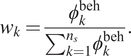 $$ {w}_k=\frac{\phi_k^{\mathrm{beh}}}{\sum_{k=1}^{n_s}{\phi}_k^{\mathrm{beh}}}. $$
Then, a resampling step is performed by randomly selecting (with replacement)
 $ {n}_s $
samples according to the weights
$ {n}_s $
samples according to the weights
 $ {w}_k $
.
$ {w}_k $
.
One common issue with the basic PF approach is the sample degeneracy problem, in which most of the particles end up having weights close to zero after some updating steps. To overcome this issue, more advanced particle filter methods, or more generally, sequential Monte Carlo methods, have been developed (Doucet et al., Reference Doucet, De Freitas and Gordon2001; Cappé et al., Reference Cappé, Godsill and Moulines2007; Chopin et al., Reference Chopin and Papaspiliopoulos2020; Kamariotis et al., Reference Kamariotis, Sardi, Papaioannou, Chatzi and Straub2023). Alternatively, Kalman filter-based methods can be employed (Li et al., Reference Li, Li, Ji and Dai2015; Song et al., Reference Song, Astroza, Ebrahimian, Moaveni and Papadimitriou2020).
4. PDT for geotechnical design and construction
4.1. Introduction
Geotechnical design is concerned with the design of structures that interact with soils. Accurately characterizing soils is challenging, as soils are spatially varying and anisotropic due to their complex geological formation process. Although the physical causes of soil formation are deterministic and obey the laws of physics, it is currently impossible to fully understand how they combine. Furthermore, it is difficult to study their variation over time with incomplete knowledge, due to the impossibility of acquiring exhaustive subsoil property information. As a result, soil formation is usually assumed to be random (Webster, Reference Webster2000). For the task of estimating geotechnical properties, Kulhawy et al., (Reference Kulhawy, Phoon, Prakoso and Hirany2006) refer to this uncertainty as the inherent soil variability.
In addition, three other sources of uncertainty exist in geotechnical engineering: measurement errors, modeling uncertainty, and statistical uncertainty (Phoon and Kulhawy, Reference Phoon and Kulhawy1999). Measurement errors emerge during data collection and are influenced by the equipment, methodologies, and personnel involved. Modeling uncertainties arise when measurement data is transformed into soil properties or quantities of interest, while statistical uncertainties are attributed to the scarcity of in-situ measurements and the methods used to extrapolate to unobserved locations.
To address the uncertainties, specific design approaches were adapted in geotechnical engineering. This includes the observational method, which was first introduced by Peck (Reference Peck1969) and has since been incorporated into Eurocode 7. It asks for a continuous design review during construction with predefined contingency actions for deviations from acceptable behavior limits (Spross and Johansson, Reference Spross and Johansson2017). This aligns with the PDT approach, which offers a systematic framework for managing the complexities and uncertainties inherent in geotechnical engineering.
In addition to uncertainties, geotechnical construction of soil data requires the integration of diverse data sources, including boreholes, cone penetration test soundings, trenches, on-site tests, and laboratory-tested site-specific samples (Zhang et al., Reference Zhang, Zhong, Wu, Guan, Yue and Wu2018). Technological advancements have increased the volume of geotechnical data collected, necessitating advanced information management tools for effective data integration and decision-making support (Chandler, Reference Chandler2011; Zhou et al., Reference Zhou, Ding and Chen2013; Phoon, Reference Phoon2019).
4.2. Application to an embankment
To demonstrate the PDT framework in geotechnical engineering, the construction of a highway on clayey soil is considered (see Figure 4) following Spross and Larsson (Reference Spross and Larsson2021) and Bismut et al. (Reference Bismut, Cotoarbă, Spross and Straub2023). A consolidation process, which causes settlements, is started by loading the clayey soil with an embankment. The consolidation converges towards an equilibrium and is dependent on the load size. Before the road on top of the embankment is constructed, the consolidation should have converged to avoid any damage to the road. To speed up the consolidation process, prefabricated vertical drains (PVDs) are installed to facilitate water drainage, and the embankment is preloaded with a surcharge. The task of engineers is to find the most cost-efficient surcharge and PVD design, which ensures that the consolidation process is finalized within a predetermined timeframe
 $ {t}_{\mathrm{max}} $
. This is a challenging task due to the large uncertainties for predicting the time and magnitude of the long-term settlement.
$ {t}_{\mathrm{max}} $
. This is a challenging task due to the large uncertainties for predicting the time and magnitude of the long-term settlement.
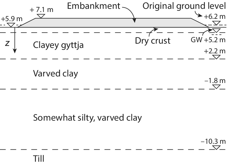
Figure 4. Cross-section of the soil under the planned embankment (from Spross and Larsson, Reference Spross and Larsson2021, CC-BY-4.0).
Spross and Larsson (Reference Spross and Larsson2021) developed a probabilistic model that describes the settlement of an embankment on top of PVDs and loaded with a surcharge over time. It is a physics-based behavioral model that is calibrated to site-specific conditions using measured data. Building on this, Bismut et al. (Reference Bismut, Cotoarbă, Spross and Straub2023) apply a risk-based framework for sequential decision-making under uncertainties to this task.
In this paper, we elaborate on how the PDT approach can be used to improve predictions and decision-making for the embankment problem. To enable this, the behavior prediction model of the surcharge is extended with Bayesian inference capabilities to integrate settlement measurements. In the following, the components of the PDT are introduced.
4.2.1. Physical state
The example application is based on the construction of the Highway 73 in southern Stockholm. It focuses on a
 $ 550\;\mathrm{m} $
road embankment constructed over a
$ 550\;\mathrm{m} $
road embankment constructed over a
 $ 0.3\;\mathrm{m} $
dry crust atop
$ 0.3\;\mathrm{m} $
dry crust atop
 $ 15.5\;\mathrm{m} $
of soft clayey soil, with a targeted embankment height of
$ 15.5\;\mathrm{m} $
of soft clayey soil, with a targeted embankment height of
 $ 1.2\;\mathrm{m} $
. The geotechnical investigation data is also taken from this project. As it is not the focus here, the PVD design is assumed to be fixed. The design details are taken from Spross and Larsson (Reference Spross and Larsson2021).
$ 1.2\;\mathrm{m} $
. The geotechnical investigation data is also taken from this project. As it is not the focus here, the PVD design is assumed to be fixed. The design details are taken from Spross and Larsson (Reference Spross and Larsson2021).
The physical state is described by the vector.
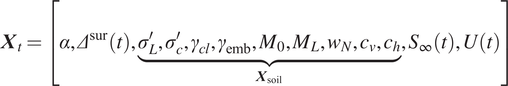 $$ {\boldsymbol{X}}_t=\left[\alpha, {\varDelta}^{\mathrm{sur}}(t),\underset{{\boldsymbol{X}}_{\mathrm{soil}}}{\underbrace{\sigma_L^{\prime },{\sigma}_c^{\prime },{\gamma}_{cl},{\gamma}_{\mathrm{emb}},{M}_0,{M}_L,{w}_N,{c}_v,{c}_h}},{S}_{\infty }(t),U(t)\right] $$
where
 $ \alpha $
are deterministic geometric boundary conditions of the embankment defined at the beginning of the project;
$ \alpha $
are deterministic geometric boundary conditions of the embankment defined at the beginning of the project;
 $ {\varDelta}^{\mathrm{sur}}(t) $
indicates the surcharge height which can change over time
$ {\varDelta}^{\mathrm{sur}}(t) $
indicates the surcharge height which can change over time
 $ t $
;
$ t $
;
 $ {\boldsymbol{X}}_{\mathrm{soil}} $
are the relevant soil properties required for the behavior prediction models used in this problem; and the long-term settlement
$ {\boldsymbol{X}}_{\mathrm{soil}} $
are the relevant soil properties required for the behavior prediction models used in this problem; and the long-term settlement
 $ {S}_{\infty }(t) $
and the degree of consolidation
$ {S}_{\infty }(t) $
and the degree of consolidation
 $ U(t) $
are quantities predicted by the behavioral models and required for deriving the quantities of interest. An in-depth explanation of the model is provided in Section 4.2.4.
$ U(t) $
are quantities predicted by the behavioral models and required for deriving the quantities of interest. An in-depth explanation of the model is provided in Section 4.2.4.
In this application,
 $ {\varphi}^{\mathrm{transition}} $
is influenced by the decision made in the previous step regarding adjustments to the surcharge height
$ {\varphi}^{\mathrm{transition}} $
is influenced by the decision made in the previous step regarding adjustments to the surcharge height
 $ {\varDelta}^{\mathrm{sur}}(t) $
and by parameters that change over time. Specifically,
$ {\varDelta}^{\mathrm{sur}}(t) $
and by parameters that change over time. Specifically,
 $ {\varDelta}^{\mathrm{sur}}(t) $
affects the long-term settlement
$ {\varDelta}^{\mathrm{sur}}(t) $
affects the long-term settlement
 $ {S}_{\infty }(t) $
. The degree of consolidation
$ {S}_{\infty }(t) $
. The degree of consolidation
 $ U(t) $
evolves over time and is mostly dependent on the PVDs.
$ U(t) $
evolves over time and is mostly dependent on the PVDs.
4.2.2. Data
Following the PDT framework, we distinguish between the property data and the behavior data.
-
a) Property data: Creating a digital representation of subsoil conditions requires soil property data, typically acquired through intrusive and non-intrusive tests. For example, borehole soundings and cone penetration tests are commonly used to classify soil types and ascertain mechanical properties. Due to the costly and intrusive nature of such tests, data availability is often limited.
In this case study, samples of soil properties were collected at different depths from a single location on the embankment, which engineers identified as problematic. These samples are used to learn the initial model, which is presented in Section 4.2.3. During the construction process, no additional property data is collected to learn the PDT, resulting in
$ {\varphi}^{\mathrm{prop}}=1 $
for
$ t>0 $
for this investigation.


-
b) Behavior data: Behavioral data in geotechnical engineering is crucial for validating and calibrating behavioral models and updating the digital state. In this case study, behavioral data is obtained from weekly measurements of the settlement
$ {z}_s(t) $
observed in the preloaded embankment. The associated measurement error is
$ \varepsilon $
, with probability density function
$ {f}_{\varepsilon } $
. The corresponding likelihood function is(4)
$$ {\phi}^{beh}={f}_{\varepsilon}\left({z}_s(t)-s(t)\right). $$
$ \varepsilon $
follows a normal distribution with mean zero and standard deviation
$ {\sigma}_{\varepsilon } $
. In the subsequent numerical investigation, three distinct scenarios with varying
$ {\sigma}_{\varepsilon } $
are analyzed to assess the impact of this parameter on the results.


4.2.3. Learning the initial digital state
As illustrated in the PDT framework in Figure 1, property data is taken as direct input in the modeling stage to create an initial digital model
 $ {d}_0 $
. Following the steps outlined in Section 2.3.4, transformation and inference are required at this stage.
$ {d}_0 $
. Following the steps outlined in Section 2.3.4, transformation and inference are required at this stage.
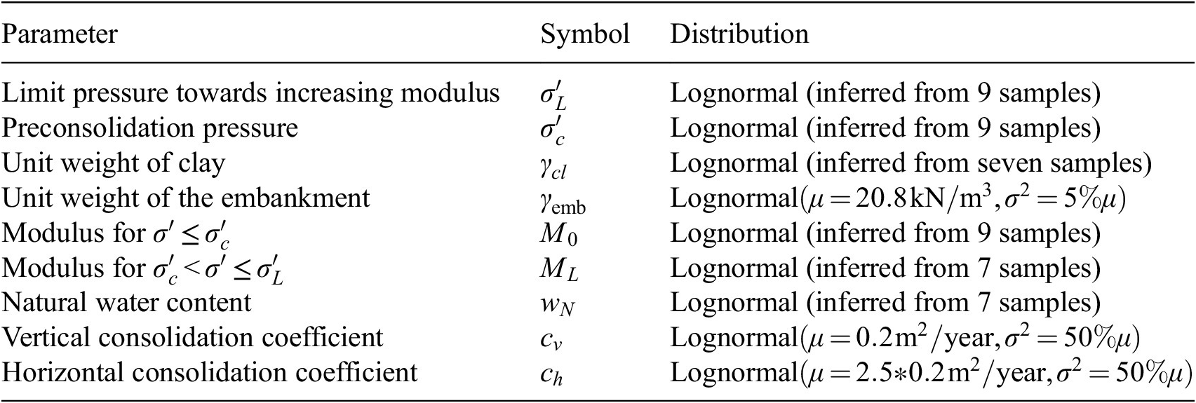
For the embankment problem, Spross and Larsson (Reference Spross and Larsson2021) describe the soil properties
 $ {\boldsymbol{X}}_{\mathrm{soil}} $
as RVs. The core modeling assumption is that soil properties vary only with depth, adopting a 1D soil model perspective. Regression models are used to learn the distribution of soil properties over depth, which is the equivalent of learning the initial digital state
$ {\boldsymbol{X}}_{\mathrm{soil}} $
as RVs. The core modeling assumption is that soil properties vary only with depth, adopting a 1D soil model perspective. Regression models are used to learn the distribution of soil properties over depth, which is the equivalent of learning the initial digital state
 $ {\boldsymbol{X}}_{\mathrm{soil}} $
are summarized in Table 1.
$ {\boldsymbol{X}}_{\mathrm{soil}} $
are summarized in Table 1.
Table 1. Geotechnical parameters modeled in the case study (Spross and Larsson, Reference Spross and Larsson2021)
4.2.4. Behavioral prediction modeling
The quantities of interest
 $ \mathbf{Q}(t) $
for this problem are the settlement
$ \mathbf{Q}(t) $
for this problem are the settlement
 $ S(t) $
and overconsolidation ratio
$ S(t) $
and overconsolidation ratio
 $ OCR(t) $
over time.
$ OCR(t) $
over time.
Geotechnical engineering commonly employs deterministic, physics-based models to predict soil behavior. For the embankment scenario, Spross and Larsson (Reference Spross and Larsson2021) utilize a traditional deterministic model for predicting the consolidation of embankments on top of PVDs and preloaded with a surcharge. The model takes as input the geotechnical stochastic parameters in
 $ {\mathbf{X}}_t $
and provides a prediction of the consolidation over time. Bismut et al. (Reference Bismut, Cotoarbă, Spross and Straub2023) extended the model to be able to account for the effect of adjusting the surcharge height during the preloading phase. This allows for more complex preloading strategies, as surcharge heights can be adapted when measurements indicate a low probability of reaching requirements. Example trajectories obtained with the model are depicted in Figure 5.
$ {\mathbf{X}}_t $
and provides a prediction of the consolidation over time. Bismut et al. (Reference Bismut, Cotoarbă, Spross and Straub2023) extended the model to be able to account for the effect of adjusting the surcharge height during the preloading phase. This allows for more complex preloading strategies, as surcharge heights can be adapted when measurements indicate a low probability of reaching requirements. Example trajectories obtained with the model are depicted in Figure 5.
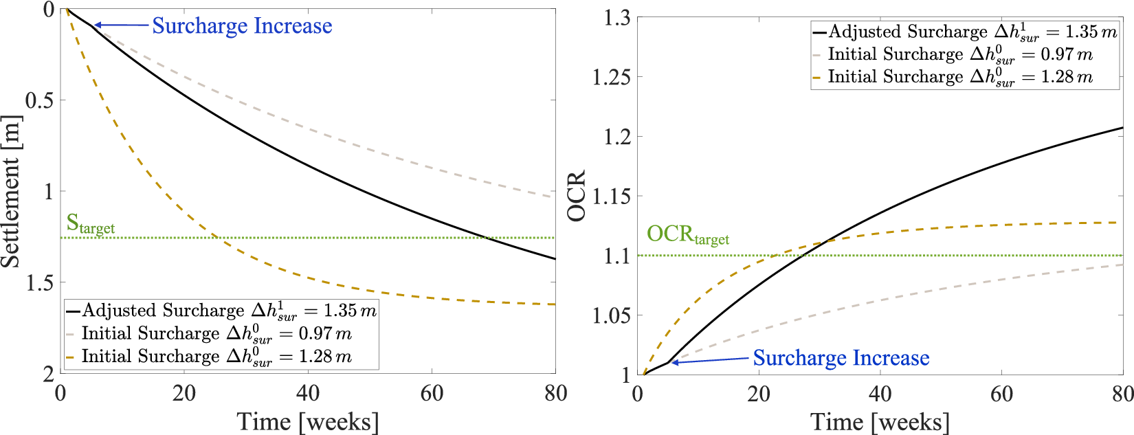
Figure 5. Three example trajectories obtained from the geotechnical model for both a) settlement and b) overconsolidation ratio over time to demonstrate the impact of adjusting the surcharge on both parameters. The grey-dashed line is a trajectory where the settlement target
 $ {s}_{\mathrm{target}} $
is not met within the maximum project time
$ {s}_{\mathrm{target}} $
is not met within the maximum project time
 $ {t}_{\mathrm{max}}=72\left[\mathrm{weeks}\right] $
. Increasing the surcharge height results in the black line trajectory, where the requirement is successfully achieved. The dashed brown line shows a trajectory where the
$ {t}_{\mathrm{max}}=72\left[\mathrm{weeks}\right] $
. Increasing the surcharge height results in the black line trajectory, where the requirement is successfully achieved. The dashed brown line shows a trajectory where the
 $ {s}_{\mathrm{target}} $
requirement is met without the need for any surcharge height adjustments.
$ {s}_{\mathrm{target}} $
requirement is met without the need for any surcharge height adjustments.
The probabilistic model is used to predict two parameters: (1)
 $ {S}_{\infty }(t) $
the predicted primary long-term settlement for
$ {S}_{\infty }(t) $
the predicted primary long-term settlement for
 $ t\to \infty $
, which is dependent on the loading capacity of soil and the preloading strategy of the embankment with
$ t\to \infty $
, which is dependent on the loading capacity of soil and the preloading strategy of the embankment with
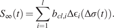 $$ {S}_{\infty }(t)=\sum \limits_{i=1}^l\;{b}_{cl,i}\Delta {\unicode{x025B}}_i\left(\Delta \sigma (t)\right). $$
It is the sum over the settlement of each layer
 $ i $
, which is given by the product between the clay layer thickness
$ i $
, which is given by the product between the clay layer thickness
 $ {b}_{cl,i} $
and the increase in strain
$ {b}_{cl,i} $
and the increase in strain
 $ \Delta {\unicode{x025B}}_i $
due to the load
$ \Delta {\unicode{x025B}}_i $
due to the load
 $ \Delta \sigma (t) $
at time
$ \Delta \sigma (t) $
at time
 $ t $
. The load is dependent on the surcharge height
$ t $
. The load is dependent on the surcharge height
 $ {h}_t $
.
$ {h}_t $
.
(2)
 $ U(t) $
, the spatially averaged degree of consolidation over time
$ U(t) $
, the spatially averaged degree of consolidation over time
 $ t $
, which is given as
$ t $
, which is given as
 $$ U(t)=1-\left[1-{U}_v(t)\right]\hskip0.24em \left[1-{U}_h(t)\right] $$
where
 $ {U}_v(t) $
and
$ {U}_v(t) $
and
 $ {U}_h(t) $
are the vertical and horizontal consolidation component. They can be obtained from Terzaghi’s consolidation theory and Hansbo’s analytical PVD model (Spross and Larsson, Reference Spross and Larsson2021).
$ {U}_h(t) $
are the vertical and horizontal consolidation component. They can be obtained from Terzaghi’s consolidation theory and Hansbo’s analytical PVD model (Spross and Larsson, Reference Spross and Larsson2021).
The distribution of the settlement over time
 $ S(t) $
is obtained as
$ S(t) $
is obtained as
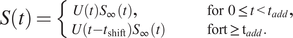 $$ S(t)=\left\{\begin{array}{cc}\hskip-2em U(t){S}_{\infty }(t),& \hskip2.3em \mathrm{for}\hskip0.35em 0\le t<{t}_{add},\\ {}U\left(t-{t}_{\mathrm{shift}}\right){S}_{\infty }(t)& \mathrm{fort}\ge {\mathrm{t}}_{add}.\end{array}\right. $$
The model is capable of considering one surcharge increment
 $ \varDelta {\sigma}_{\mathrm{add}} $
at time
$ \varDelta {\sigma}_{\mathrm{add}} $
at time
 $ {t}_{add} $
. This results in the total embankment load
$ {t}_{add} $
. This results in the total embankment load
 $$ \varDelta \sigma (t)=\varDelta {\unicode{x03C3}}_{\mathrm{emb}}+\varDelta {\sigma}_{\mathrm{sur}}+\varDelta {\sigma}_{\mathrm{add}}\hskip6.00em \mathrm{for}\hskip0.35em t>{t}_{\mathrm{add}}. $$
The parameter
 $ {t}_{\mathrm{shift}} $
is required to reflect the accelerated consolidation process due to an increased load, resulting in a larger
$ {t}_{\mathrm{shift}} $
is required to reflect the accelerated consolidation process due to an increased load, resulting in a larger
 $ {S}_{\infty } $
. For details on how to obtain it, we refer to Bismut et al. (Reference Bismut, Cotoarbă, Spross and Straub2023).
$ {S}_{\infty } $
. For details on how to obtain it, we refer to Bismut et al. (Reference Bismut, Cotoarbă, Spross and Straub2023).
The overconsolidation ratio
 $ \mathrm{OCR} $
at time
$ \mathrm{OCR} $
at time
 $ t $
is given as
$ t $
is given as
 $$ \mathrm{OCR}(t)=\frac{\sigma_0^{\prime }+U(t)\varDelta {\sigma}_{\mathrm{sur}}+\varDelta U(t)\varDelta {\sigma}_{\mathrm{add}}}{\sigma_0^{\prime }+U(t)\varDelta {\sigma}_{\mathrm{emb}}}, $$
and describes the ratio between preconsolidation stress due to the embankment load
 $ \varDelta {\sigma}_{\mathrm{emb}} $
and current stress due to the added preloading
$ \varDelta {\sigma}_{\mathrm{emb}} $
and current stress due to the added preloading
 $ \varDelta {\sigma}_{\mathrm{sur}}+\varDelta {\sigma}_{\mathrm{add}} $
.
$ \varDelta {\sigma}_{\mathrm{sur}}+\varDelta {\sigma}_{\mathrm{add}} $
.
 $ \Delta U(t) $
is again required to account for the accelerated consolidation process due to the load increase. We refer to (Bismut et al., Reference Bismut, Cotoarbă, Spross and Straub2023) for a detailed explanation of how it is calculated.
$ \Delta U(t) $
is again required to account for the accelerated consolidation process due to the load increase. We refer to (Bismut et al., Reference Bismut, Cotoarbă, Spross and Straub2023) for a detailed explanation of how it is calculated.
Following the above model, the quantities of interest in
 $ \mathbf{Q}(t) $
are a deterministic function of
$ \mathbf{Q}(t) $
are a deterministic function of
 $ {\mathbf{X}}_t $
,
$ {\mathbf{X}}_t $
,
 $ \mathbf{Q}(t)=q\left({\mathbf{X}}_t\right) $
. Therefore,
$ \mathbf{Q}(t)=q\left({\mathbf{X}}_t\right) $
. Therefore,
 $ {\varphi}^{\mathrm{pred}} $
is expressed through the Dirac delta function as
$ {\varphi}^{\mathrm{pred}} $
is expressed through the Dirac delta function as
 $ {\varphi}^{\mathrm{pred}}=\delta \left({\boldsymbol{Q}}_t-q\left({\boldsymbol{X}}_t\right)\right) $
.
$ {\varphi}^{\mathrm{pred}}=\delta \left({\boldsymbol{Q}}_t-q\left({\boldsymbol{X}}_t\right)\right) $
.
4.2.5. Behavioral prediction updating
In this study, the basic particle filter (see Section 3) is used to update the distribution of the settlement over time with weekly settlement measurements described in Section 4.2.2. As expected, we also observe the sample degeneracy problem during the updating process. However, as we show in Section 5, the accuracy of the approach in this case suffices for improving the decision-making process.
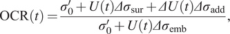
In Figure 6 the prior and posterior of
 $ S(t) $
obtained with particle filtering for a measurement at
$ S(t) $
obtained with particle filtering for a measurement at
 $ t=20\left[\mathrm{weeks}\right] $
is illustrated.
$ t=20\left[\mathrm{weeks}\right] $
is illustrated.
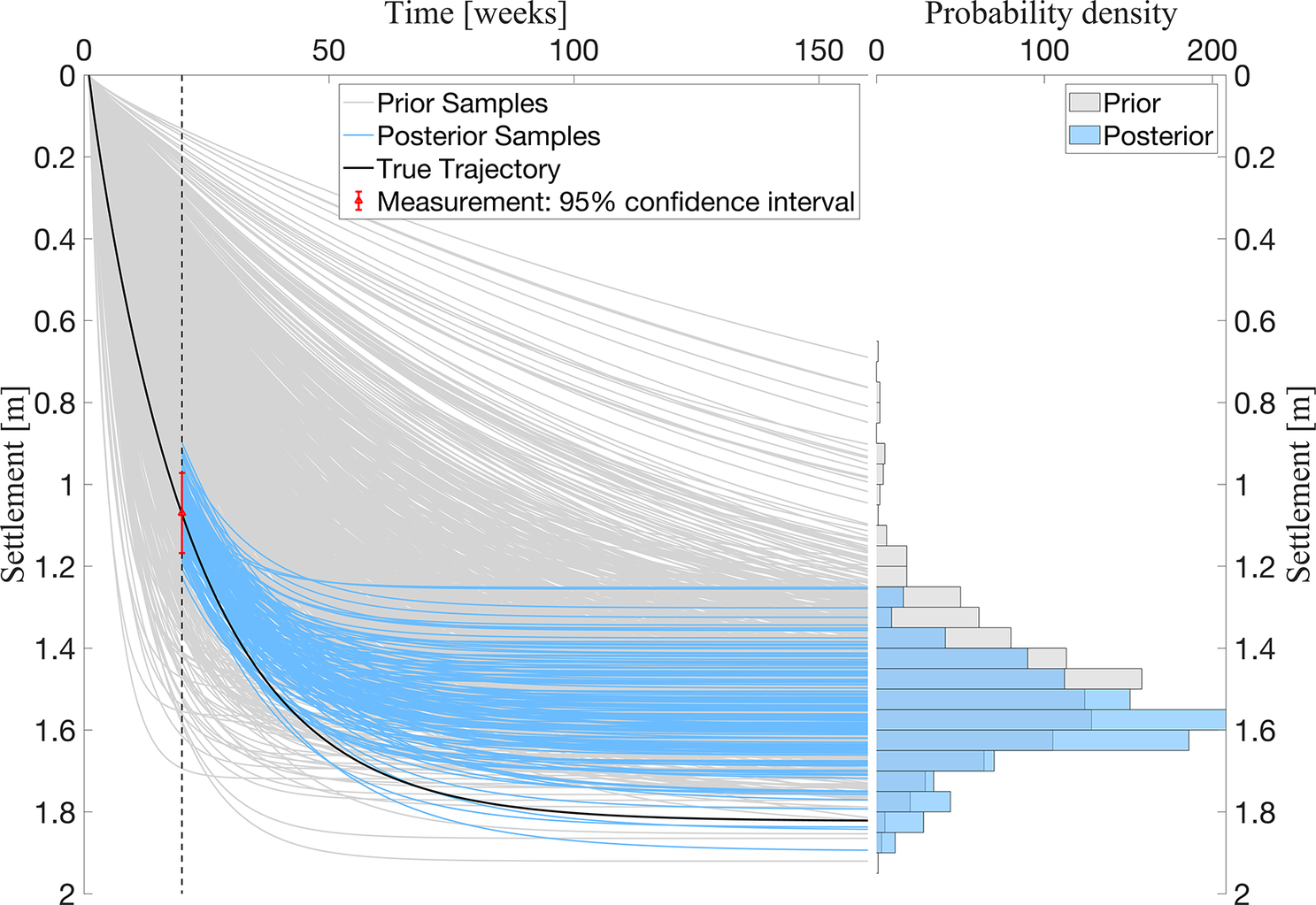
Figure 6.
 $ \mathrm{10,000} $
trajectory samples obtained with the probabilistic model for an initial surcharge
$ \mathrm{10,000} $
trajectory samples obtained with the probabilistic model for an initial surcharge
 $ {h}_0=0.9\;\mathrm{m} $
. On the left side, their evolution over time is illustrated. The posterior (highlighted in blue) is obtained for a measurement
$ {h}_0=0.9\;\mathrm{m} $
. On the left side, their evolution over time is illustrated. The posterior (highlighted in blue) is obtained for a measurement
 $ {z}_s\left(t=20\; weeks\right)=1.08\;\mathrm{m} $
. Measurement errors are modeled as a standard normal distribution
$ {z}_s\left(t=20\; weeks\right)=1.08\;\mathrm{m} $
. Measurement errors are modeled as a standard normal distribution
 $ {\sigma}_{\varepsilon }=5\;\mathrm{cm} $
and added to the measurement. The histogram on the right illustrates both the prior and posterior of the distribution of
$ {\sigma}_{\varepsilon }=5\;\mathrm{cm} $
and added to the measurement. The histogram on the right illustrates both the prior and posterior of the distribution of
 $ S $
at
$ S $
at
 $ t=160 $
.
$ t=160 $
.
4.2.6. Decision making
-
a) Decisions: This application does not involve decisions
$ {e}_t $
to collect additional information, as a decision to collect weekly settlement measurements is taken a priori.Decisions are taken on the surcharge height. The first decision at time zero is the initial surcharge height
$ {a}_0\hskip0.36em =\hskip0.36em \left[{h}_0\right] $
. In subsequent time steps, the decision alternatives are
$ {a}_t=[\mathrm{do}\hskip0.35em \mathrm{nothing},\hskip0.35em \mathrm{adjust}\ \mathrm{surcharge}\ \mathrm{height}\hskip0.35em \mathrm{by}\;{h}_1] $
. -
b) Requirements: For the embankment problem, Spross and Larsson (Reference Spross and Larsson2021) specify requirements for the settlement and OCR at the time of unloading
$ {t}_{\mathrm{max}} $
. First,(10)where
$$ S\left({t}_{\mathrm{max}}\right)\le {s}_{\mathrm{target}}, $$
$ {s}_{\mathrm{target}} $
represents the settlement threshold. This criterion ensures that residual primary consolidation remains within acceptable serviceability limits after unloading. This requirement is considered crucial and the embankment can only be unloaded when it is fulfilled. Not meeting this requirement at
$ {t}_{\mathrm{max}} $
results in project delay and penalties.
The OCR requirement aims to prevent creep settlements after the road is taken into service:
(11)with
$$ \mathrm{OC}\mathrm{R}\left({t}_{\mathrm{max}}\right)\ge \mathrm{OC}{\mathrm{R}}_{\mathrm{target}} $$
$ \mathrm{OC}{\mathrm{R}}_{\mathrm{target}}=1.10 $
as specified in the general technical requirements and guidance for geotechnical works issued by the Swedish Transport Administration (Spross and Larsson, Reference Spross and Larsson2021). Failing to meet the OCR criterion can deteriorate road quality and reduce its lifespan, leading to bumps in the road, cracks and accelerated wear.
-
c) Cost function: Following Bismut et al. (Reference Bismut, Cotoarbă, Spross and Straub2023), the cost function is
(12)where
$$ {C}_{\mathrm{tot}}={\sum}_i{C}_{\mathrm{sur},i}+{C}_{\mathrm{delay}}+{C}_{\mathrm{OCR}}, $$
$ {C}_{\mathrm{sur},i} $
quantifies the costs of the surcharge (e.g., material, equipment, and labor costs), with
$ i=1 $
representing the initial construction costs and
$ i=2 $
the costs for increasing the surcharge;
$ {C}_{\mathrm{delay}} $
quantifies the penalty if
$ {s}_{\mathrm{target}} $
is not reached in time; and
$ {C}_{\mathrm{OCR}} $
quantifies the penalty of not reaching
$ OC{R}_{\mathrm{target}} $
at time of unloading. For the full details of the cost function parameters, we refer to (Bismut et al., Reference Bismut, Cotoarbă, Spross and Straub2023).
In the PDT, the cost function is equivalent to the negative reward
$ {\mathbf{R}}_t $
and the components of the summation in Equation (12) are a function of
$ {\boldsymbol{X}}_{0:t\max } $
and
$ {\boldsymbol{a}}_{0:t\max } $
.
$ {C}_{\mathrm{sur},i} $
depends on the surcharge decision
$ {a}_t $
, whereas
$ {C}_{\mathrm{delay}} $
and
$ {C}_{\mathrm{OCR}} $
depend on quantities of interest at time
$ {t}_{\mathrm{max}} $
, i.e.,
$ S\left({t}_{\mathrm{max}}\right) $
and
$ \mathrm{OCR}\left({t}_{\mathrm{max}}\right) $
. To make this dependence explicit, we use the notation
$ {C}_{\mathrm{tot}}\left({\boldsymbol{X}}_{0:t\max },{\boldsymbol{a}}_{0:t\max}\right) $
in the following. -
d) Optimal decision: The objective of the decision optimization is to find the sequence of actions, i.e., surcharge loading that results in the lowest expected cost. The actions are defined by a decision strategy
$ \mathcal{S} $
, which consists of a set of policies
$ {\pi}_t $
that define the action
$ {a}_t $
to take at time
$ t $
in function of the current digital state
$ {d}_t $
, i.e.,
$ {a}_t={\pi}_t\left({d}_t\right) $
. The goal is to find the optimal strategy.A heuristic approach is chosen to solve this decision problem (Bismut and Straub, Reference Bismut and Straub2021). It reduces the complexity of the problem by describing the strategy
$ \mathcal{S} $
through a parametric function
$ {\mathcal{S}}_{\mathbf{w}} $
, where
$ \mathbf{w}=\left[{w}_1,{w}_2,\dots {w}_n\right] $
are the heuristic parameters.The optimal heuristic strategy for a given heuristic function is defined by parameters
(13)and aims to find the minimal expected cost.
$$ {\boldsymbol{w}}_{\mathrm{opt}}=\mathit{\arg}\underset{\boldsymbol{w}}{\mathit{\min}}\unicode{x1D53C}\left[{C}_{tot}\Big({\boldsymbol{X}}_{0:t\max },{S}_{\boldsymbol{w}}\left({\boldsymbol{D}}_{0:t\max}\right)\Big)\right] $$
Monte Carlo simulation is used to obtain an approximation of the objective function of Equation (13).
$ {n}_{\mathrm{MC}} $
sample trajectories for a given surcharge height are simulated using the probabilistic geotechnical model. The MC approximation for a given set of heuristic parameters
$ \mathbf{w} $
is given as(14)wherein
$$ \mathcal{E}\left[{C}_{\mathrm{tot}}\Big({\boldsymbol{X}}_{0:t\max },{S}_{\boldsymbol{w}}\left({\boldsymbol{D}}_{0:t\max}\right)\Big)\right]\approx \frac{1}{n_{\mathrm{MC}}}\sum_{k=1}^{n_{\mathrm{MC}}}{C}_{\mathrm{tot}}({\boldsymbol{X}}_{0:t\max}^{(k)},{S}_{\boldsymbol{w}}({\boldsymbol{D}}_{0:t\max}^{(k)})) $$
$ {\boldsymbol{X}}_{0:t\max}^{(k)} $
are the
$ k=1:{n}_{\mathrm{MC}} $
sample trajectories of the true state and
$ {\boldsymbol{D}}_{0:t\max}^{(k)} $
are the corresponding samples of the digital state.
To solve Equation (13), the cross-entropy (CE) optimization is used (Kroese et al., Reference Kroese, Porotsky and Rubinstein2006; Bismut et al., Reference Bismut, Straub and Pandey2022). It is an optimization method tailored to noisy optimization problems. For details on the employed CE algorithm, we refer to Bismut et al. (Reference Bismut, Cotoarbă, Spross and Straub2023).


4.2.7. Summary
Figure 7 shows the influence diagram of the general PDT tailored to this specific application. Here, the physical state
 $ {\mathbf{X}}_t $
includes all the parameters identified as necessary to describe the embankment and its settlement over time. The state is learned in the initial stage from collected property data samples of
$ {\mathbf{X}}_t $
includes all the parameters identified as necessary to describe the embankment and its settlement over time. The state is learned in the initial stage from collected property data samples of
 $ {\boldsymbol{X}}_{\mathrm{soil}} $
. These soil properties are the input of the probabilistic settlement model by Spross and Larsson (Reference Spross and Larsson2021) for the prediction of the quantities of interest
$ {\boldsymbol{X}}_{\mathrm{soil}} $
. These soil properties are the input of the probabilistic settlement model by Spross and Larsson (Reference Spross and Larsson2021) for the prediction of the quantities of interest
 $ \mathbf{Q}(t)=\left[S(t), OCR(t)\right] $
. Behavioral data for this problem consists of measurements of the settlement
$ \mathbf{Q}(t)=\left[S(t), OCR(t)\right] $
. Behavioral data for this problem consists of measurements of the settlement
 $ {\mathbf{z}}_s(t) $
, which are used to update the physical state
$ {\mathbf{z}}_s(t) $
, which are used to update the physical state
 $ {\mathbf{X}}_t $
to enhance the prediction accuracy of the quantities of interest. Decisions on the surcharge height
$ {\mathbf{X}}_t $
to enhance the prediction accuracy of the quantities of interest. Decisions on the surcharge height
 $ {a}_t $
are based on the posterior predictions and directly affect the total expected cost
$ {a}_t $
are based on the posterior predictions and directly affect the total expected cost
 $ {C}_{\mathrm{tot}} $
. Heuristics for decision optimization of the preloading strategy are employed to identify actions that minimize the costs over the lifecycle of the embankment.
$ {C}_{\mathrm{tot}} $
. Heuristics for decision optimization of the preloading strategy are employed to identify actions that minimize the costs over the lifecycle of the embankment.
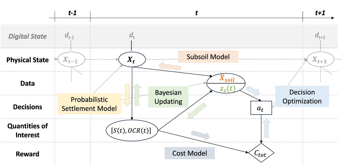
Figure 7. . The PDT influence diagram of Figure 2, adapted to the considered application case.
5. Numerical investigation
5.1. Model setup
The numerical investigation is performed for the embankment of a highway section constructed in southern Stockholm, Sweden, introduced in Section 4.2.1. The potential of the PDT, illustrated in Figure 7, for the optimization of preloading strategies is investigated. The settlement target
 $ {s}_{\mathrm{target}}=1.27\;\mathrm{m} $
is according to Spross and Larsson (Reference Spross and Larsson2021). The cost function parameters are adopted from Bismut et al. (Reference Bismut, Cotoarbă, Spross and Straub2023).
$ {s}_{\mathrm{target}}=1.27\;\mathrm{m} $
is according to Spross and Larsson (Reference Spross and Larsson2021). The cost function parameters are adopted from Bismut et al. (Reference Bismut, Cotoarbă, Spross and Straub2023).
5.2. Decision heuristic
In this study, we introduce a heuristic
 $ {\mathcal{S}}_{\mathbf{w}} $
that leverages the PDT to improve decision-making for the embankment construction. This heuristic is later compared to heuristics established in previous work (Bismut et al., Reference Bismut, Cotoarbă, Spross and Straub2023; Cotoarbă et al., Reference Cotoarbă, Bismut, Spross and Straub2023), which are based on data rather than model predictions.
$ {\mathcal{S}}_{\mathbf{w}} $
that leverages the PDT to improve decision-making for the embankment construction. This heuristic is later compared to heuristics established in previous work (Bismut et al., Reference Bismut, Cotoarbă, Spross and Straub2023; Cotoarbă et al., Reference Cotoarbă, Bismut, Spross and Straub2023), which are based on data rather than model predictions.
An initial surcharge height
 $ {a}_0 $
is established at the start of the project. Subsequently, the settlement induced by the surcharge is monitored at weekly intervals, denoted as
$ {a}_0 $
is established at the start of the project. Subsequently, the settlement induced by the surcharge is monitored at weekly intervals, denoted as
 $ t $
. Following each observation, Bayesian updating of the physical state
$ t $
. Following each observation, Bayesian updating of the physical state
 $ {\mathbf{X}}_t $
is performed as detailed in Section 4.2.5. Data is collected until the standard deviation of the updated belief falls below a predefined threshold
$ {\mathbf{X}}_t $
is performed as detailed in Section 4.2.5. Data is collected until the standard deviation of the updated belief falls below a predefined threshold
 $ {\operatorname{cov}}_{th} $
. Utilizing the posterior belief of the settlement
$ {\operatorname{cov}}_{th} $
. Utilizing the posterior belief of the settlement
 $ S\left({t}_{\mathrm{max}}\right) $
, the probability of not achieving
$ S\left({t}_{\mathrm{max}}\right) $
, the probability of not achieving
 $ {s}_{\mathrm{target}} $
by the time
$ {s}_{\mathrm{target}} $
by the time
 $ {t}_{\mathrm{max}} $
is assessed. If this probability is higher than a probability threshold
$ {t}_{\mathrm{max}} $
is assessed. If this probability is higher than a probability threshold
 $ {\mathrm{P}}_{th} $
, the surcharge height is increased by
$ {\mathrm{P}}_{th} $
, the surcharge height is increased by
 $ {h}_{\mathrm{sur}} $
, which is defined as the smallest value that ensures that the probability
$ {h}_{\mathrm{sur}} $
, which is defined as the smallest value that ensures that the probability
 $ \mathit{\Pr}\left[S\left({t}_{\mathrm{max}}\right)>{s}_{\mathrm{target}}\right] $
falls below this threshold.
$ \mathit{\Pr}\left[S\left({t}_{\mathrm{max}}\right)>{s}_{\mathrm{target}}\right] $
falls below this threshold.
An example outcome of the PDT for the described scenario is depicted in Figure 8. The first panel shows the evolution of the surcharge height over time
 $ t $
. The second panel outlines the belief state evolution of the settlement as observations are collected. Measurements continue until
$ t $
. The second panel outlines the belief state evolution of the settlement as observations are collected. Measurements continue until
 $ t=16 $
when the confidence interval (CI) for settlement predictions falls below the threshold
$ t=16 $
when the confidence interval (CI) for settlement predictions falls below the threshold
 $ {\operatorname{cov}}_{th} $
. This indicates that prediction uncertainty has been sufficiently minimized for decision-making. Consequently, the surcharge height is increased to ensure that the predicted probability of not reaching
$ {\operatorname{cov}}_{th} $
. This indicates that prediction uncertainty has been sufficiently minimized for decision-making. Consequently, the surcharge height is increased to ensure that the predicted probability of not reaching
 $ {s}_{\mathrm{target}} $
is lower than
$ {s}_{\mathrm{target}} $
is lower than
 $ {\mathrm{P}}_{th} $
. The third and fourth panels depict the evolution of the
$ {\mathrm{P}}_{th} $
. The third and fourth panels depict the evolution of the
 $ 95\% $
CI together with the true value for the quantities of interest
$ 95\% $
CI together with the true value for the quantities of interest
 $ S\left({t}_{max}\right) $
and
$ S\left({t}_{max}\right) $
and
 $ OCR\left({t}_{\mathrm{max}}\right) $
. They demonstrate that the mitigation action was effective, as
$ OCR\left({t}_{\mathrm{max}}\right) $
. They demonstrate that the mitigation action was effective, as
 $ {s}_{\mathrm{target}} $
is now reached within the designated project time.
$ {s}_{\mathrm{target}} $
is now reached within the designated project time.
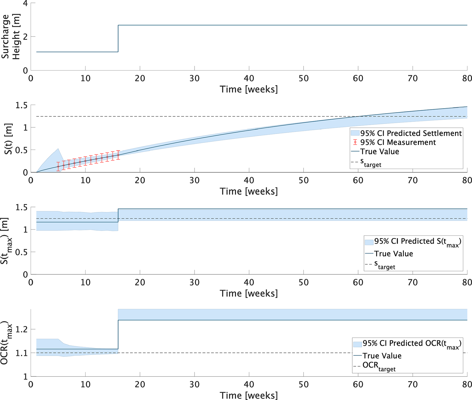
Figure 8. The PDT dashboard for an example trajectory with the following heuristic parameters
 $ \mathbf{w}=\left[{h}_0=1.09\hskip0.22em m,{\mathit{\operatorname{cov}}}_{th}=0.05,{P}_{th}=0.43\right] $
.
$ \mathbf{w}=\left[{h}_0=1.09\hskip0.22em m,{\mathit{\operatorname{cov}}}_{th}=0.05,{P}_{th}=0.43\right] $
.
To identify the optimal heuristic parameters
 $ \mathbf{w}=\left[{h}_0,{\operatorname{cov}}_{th},{\mathrm{P}}_{th}\right] $
that minimize the expected total cost introduced in Equation (13) a CE optimization is performed.
$ \mathbf{w}=\left[{h}_0,{\operatorname{cov}}_{th},{\mathrm{P}}_{th}\right] $
that minimize the expected total cost introduced in Equation (13) a CE optimization is performed.
5.3. Computational details
For the CE method, specific values are set as follows: number of CE samples per iteration
 $ {n}_{\mathrm{CE}}=1{0}^2 $
, maximum number of iterations
$ {n}_{\mathrm{CE}}=1{0}^2 $
, maximum number of iterations
 $ {n}_E=50 $
, number of MCS samples for each CE set
$ {n}_E=50 $
, number of MCS samples for each CE set
 $ {n}_{\mathrm{MC}}=1{0}^2 $
and number of samples considered for Bayesian updating
$ {n}_{\mathrm{MC}}=1{0}^2 $
and number of samples considered for Bayesian updating
 $ {n}_{\mathrm{BU}}=1{0}^2 $
. The expected cost associated with the optimized heuristic parameters is assessed in a more extensive evaluation involving
$ {n}_{\mathrm{BU}}=1{0}^2 $
. The expected cost associated with the optimized heuristic parameters is assessed in a more extensive evaluation involving
 $ {n}_{\mathrm{MC}}=5\ast 1{0}^3 $
Monte Carlo samples. The optimization is conducted using a computing setup comprising a 10-core 3.2 GHz CPU and a 10-core GPU, equipped with 32GB of memory, resulting in a total computation time of 21 minutes. This offline computation was executed once per optimization run.
$ {n}_{\mathrm{MC}}=5\ast 1{0}^3 $
Monte Carlo samples. The optimization is conducted using a computing setup comprising a 10-core 3.2 GHz CPU and a 10-core GPU, equipped with 32GB of memory, resulting in a total computation time of 21 minutes. This offline computation was executed once per optimization run.
5.4. Results
5.4.1. Varying measurement error
The proposed heuristic is applied for three scenarios, distinguished by the standard deviation of the measurement error, which varies between
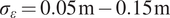 $ {\sigma}_{\varepsilon }=0.05\;\mathrm{m}-0.15\;\mathrm{m} $
. Table 2 presents the resulting expected costs and parameters of the optimized heuristic for each scenario.
$ {\sigma}_{\varepsilon }=0.05\;\mathrm{m}-0.15\;\mathrm{m} $
. Table 2 presents the resulting expected costs and parameters of the optimized heuristic for each scenario.
Table 2. Optimal heuristic parameters and associated expected costs for the three scenarios with varying measurement errors investigated in this work
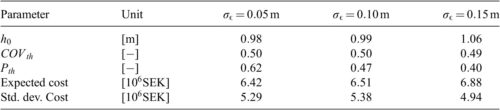
A side-to-side breakdown of the expected costs for each scenario, provided in Figure 9, indicates similar performance for measurement errors
 $ {\sigma}_{\varepsilon }=0.05\;\mathrm{m} $
and
$ {\sigma}_{\varepsilon }=0.05\;\mathrm{m} $
and
 $ {\sigma}_{\varepsilon }=0.10\;\mathrm{m} $
, with a noticeable increase in expected costs for
$ {\sigma}_{\varepsilon }=0.10\;\mathrm{m} $
, with a noticeable increase in expected costs for
 $ {\sigma}_{\varepsilon }=0.15\;\mathrm{m} $
. However, the latter case results in a higher expected cost, but with a lower standard deviation. This is probably due to the low robustness of the CE method encountered for this problem. Nonetheless, the heuristic consistently extracts actionable information for decision-making across all scenarios.
$ {\sigma}_{\varepsilon }=0.15\;\mathrm{m} $
. However, the latter case results in a higher expected cost, but with a lower standard deviation. This is probably due to the low robustness of the CE method encountered for this problem. Nonetheless, the heuristic consistently extracts actionable information for decision-making across all scenarios.
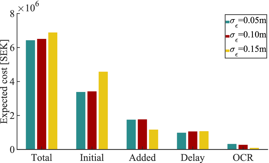
Figure 9. Cost breakdown of the best results for each scenario for the proposed heuristic.
Furthermore, Figure 10 showcases the distribution of settlement and OCR at the time of unloading across all scenarios. We note that for each scenario, the heuristic ensures compliance with both
 $ {s}_{\mathrm{target}} $
and
$ {s}_{\mathrm{target}} $
and
 $ OC{R}_{\mathrm{target}} $
requirements upon unloading for most cases. The peaks of the probability distributions are close to the requirements, indicating the efficacy of the heuristic in identifying solutions that not only meet the specified criteria but also optimize cost efficiency.
$ OC{R}_{\mathrm{target}} $
requirements upon unloading for most cases. The peaks of the probability distributions are close to the requirements, indicating the efficacy of the heuristic in identifying solutions that not only meet the specified criteria but also optimize cost efficiency.
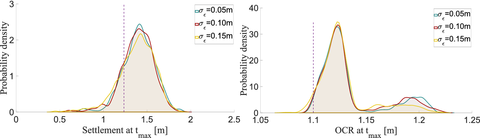
Figure 10. Kernel representation of the a) settlement and b) OCR at time of unloading
 $ {t}_{\mathrm{max}} $
for the best results of each scenario for the proposed heuristic.
$ {t}_{\mathrm{max}} $
for the best results of each scenario for the proposed heuristic.
 $ 10\mathrm{0,000} $
samples where obtained with the parameters listed in Table 3.
$ 10\mathrm{0,000} $
samples where obtained with the parameters listed in Table 3.
5.4.2. Comparison with state-of-the-art
In previous work, measurement errors were only assumed in Cotoarbă et al. (Reference Cotoarbă, Bismut, Spross and Straub2023), and even minimal measurement errors significantly impacted the efficiency of the employed heuristics because they were based on observations directly instead of predictive modeling. These heuristics worked well for ideal conditions, where measurement errors were omitted.
The comparison summarized in Table 3 shows the results for the current heuristic against the results Heuristic 1 and Heuristic 4 from previous studies by Bismut et al. (Reference Bismut, Cotoarbă, Spross and Straub2023); Cotoarbă et al. (Reference Cotoarbă, Bismut, Spross and Straub2023). Heuristic 1 serves as the reference case and offers a simplistic decision framework that optimizes only the initial surcharge height without the possibility for subsequent adjustments. This can be considered the state-of-the-art, as a Monte Carlo Simulation is used for optimization. Heuristic 4 adopts a regression model, trained on available measurements at the decision time to predict
 $ {S}_{t_{\mathrm{max}}} $
. The surcharge height is adjusted according to the difference between the prediction and
$ {S}_{t_{\mathrm{max}}} $
. The surcharge height is adjusted according to the difference between the prediction and
 $ {s}_{\mathrm{target}} $
. For Heuristic 4 the largest measurement error that was considered is
$ {s}_{\mathrm{target}} $
. For Heuristic 4 the largest measurement error that was considered is
 $ {\sigma}_{\varepsilon }=0.03\;\mathrm{m} $
.
$ {\sigma}_{\varepsilon }=0.03\;\mathrm{m} $
.
Table 3. Comparison between best results for probabilistic-digital-twin-based heuristics and two heuristics from previous work
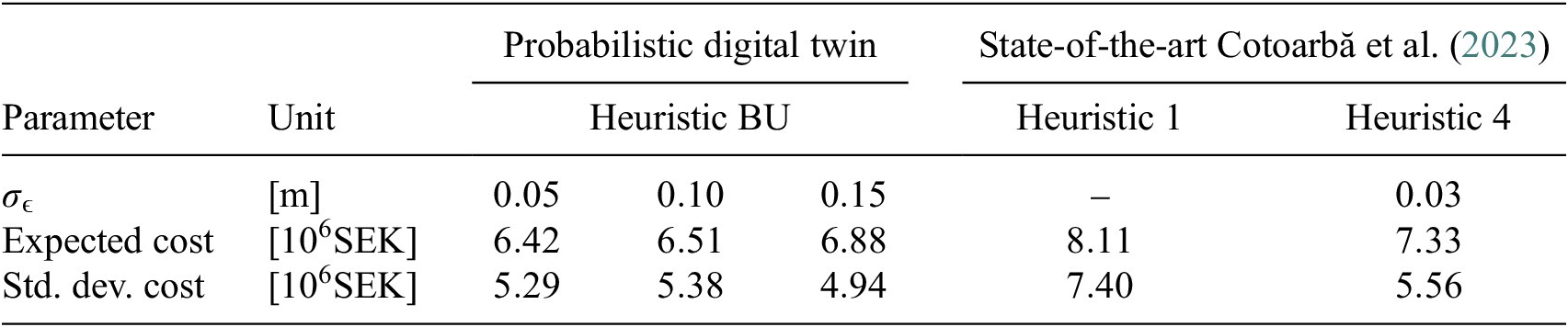
In comparison with previous work, even the worst-case scenario for the PDT-based heuristic with
 $ {\sigma}_{\varepsilon }=0.15\;\mathrm{m} $
outperforms Heuristic 4 with
$ {\sigma}_{\varepsilon }=0.15\;\mathrm{m} $
outperforms Heuristic 4 with
 $ {\sigma}_{\varepsilon }=0.03\;\mathrm{m} $
, achieving a reduction in the expected total costs by
$ {\sigma}_{\varepsilon }=0.03\;\mathrm{m} $
, achieving a reduction in the expected total costs by
 $ 6-13\% $
and up to
$ 6-13\% $
and up to
 $ 20\% $
compared to the state-of-the-art. Additionally, the standard deviation of the cost is reduced by up to
$ 20\% $
compared to the state-of-the-art. Additionally, the standard deviation of the cost is reduced by up to
 $ 40\% $
and shows that by incorporating Bayesian learning, variability in the final expected cost can be reduced.
$ 40\% $
and shows that by incorporating Bayesian learning, variability in the final expected cost can be reduced.
6. Discussion
The presented PDT example application demonstrates the potential of applying Bayesian learning to optimize geotechnical construction under uncertainty and sequential data input. The approach effectively extracts information from noisy data, enables more accurate predictions of settlements and OCR, and identifies cost-efficient construction strategies using a heuristic strategy optimization.
However, while promising, this first implementation of the PDT has several limitations. First, property data is only used for initial model development due to limited availability. The model can be easily extended to update the digital state as new property data (e.g., soil samples) becomes available. Second, extending the subsoil model from 1D to 3D would enable more accurate representation of soil conditions. Third, the implementation currently considers only one behavioral prediction model (soil settlement over time under load), whereas the full potential of the PDT approach lies in integrating multiple models. Increasing PDT complexity in this way will require the investigation of more efficient data models and methods.
Despite these limitations and challenges, this work demonstrates the potential of the PDT approach to enhance geotechnical design and construction decision-making compared to traditional methods. The PDT integrates both traditional and novel geotechnical design and construction methods. The adoption of stochastic parameter description enables the integration of Bayesian probabilistic models and learning from diverse data sources. This aligns with established geotechnical design practices, such as the observational method outlined in Eurocode 7 (CEN EN, 1997–1:2004). In addition to model updating, the probabilistic description allows the use of existing optimization approaches for sequential decision-making under uncertainties.
While this study showcases the implementation of a PDT for embankment design and construction, its application is not limited to this context. The framework can be extended to various geotechnical engineering challenges, including excavation pits, tunneling, and offshore foundations. As discussed in Section 2.3.2, a thorough requirement analysis is essential to identify the appropriate prediction models and their required input data. The choice between physics-based models and surrogate models involves a trade-off between accuracy and computational efficiency. The main challenge lies in the practical implementation and seamless integration of these models with decision-optimization processes, which remains a non-trivial task. Future research should focus on addressing these challenges.
A key strength of the Bayesian approach within the PDT framework is its ability to adapt to varying levels of data availability and uncertainty. By integrating prior knowledge and continuously refining predictions as new measurements become available, traditional Bayesian methods enhance decision-making reliability. In cases where data is particularly scarce or noisy, non-informative prior distributions constrained by engineering judgment can be used. This adaptability makes the PDT framework a valuable tool for geotechnical design and assessment, even in complex environments where data uncertainty is a persistent challenge.
7. Conclusion
This study demonstrates the potential of the PDT framework to advance geotechnical design and construction by integrating probabilistic methods within a DT environment. By systematically incorporating uncertainties and continuously updating models with monitoring data, the PDT enhances decision-making and enables cost-efficient design optimization under uncertainty. Its effectiveness is illustrated through an embankment case study, where the framework improved predictions and proposed cost reductions compared to traditional approaches.
The PDT represents a novel advancement in geotechnical design and construction, overcoming barriers to the adoption of probabilistic methods in practice. By complementing established approaches such as the observational method, it provides a structured framework for managing uncertainties and tailoring models to site-specific conditions, making probabilistic design more accessible.
Future research is needed to better understand the implementation of the proposed framework for more complex applications. A key challenge is the integration of models for subsoil characterization and behavior prediction into a centralized platform while ensuring their connection with decision-optimization processes. Addressing these challenges will be crucial for realizing the full potential of the PDT in geotechnical design and construction.
Data availability statement
Data availability is not applicable to this article as no new data were created or analyzed in this study.
Author contribution
Conceptualization: D.C., D.S., I.S.; Formal analysis: D.C.; Funding acquisition: I.S.; Methodology: D.C., D.S., I.S.; Software: D.C.; Visualization: D.C.; Writing—original draft: D.C.; Writing— review and editing: D.C., D.S., I.S. All authors approved the final submitted draft.
Funding statement
This research is supported by the TUM Georg Nemetschek Institute Artificial Intelligence for the Built World.
Competing interests
The authors declare none.


 Open access
Comments
No Comments have been published for this article.