Introduction
Influenza, commonly known as flu, circulates worldwide and places a substantial burden on people's health every year. The flu outbreak resulted in approximately 3–5 million annual cases of severe illness and 250 000–500 000 deaths [1]. In the USA, annual flu outbreak led to an average of 610 660 life-years lost, 3.1 million hospitalised days and 31.4 million outpatient visits. The total economic burden of annual flu outbreak using projected statistical life values amounted to $87.1 billion [Reference Molinari2]. Flu is one of the costliest epidemics worldwide.
The flu vaccine is one of the best ways to reduce the risk of getting sick with flu and spreading it to others [3]. During the 2015–2016 flu season, flu vaccine prevented an estimated 5.1 million illnesses, 2.5 million medical visits, 71 000 hospitalisations and 3000 pneumonia and influenza deaths [3]. However, because flu virus undergoes high mutation rates and frequent genetic re-assortment [Reference Lubeck, Schulman and Palese4–Reference Suárez, Valcárcel and Ortín6], manufacturing flu vaccine suffers from a complicated process every year. In Februaries, World Health Organization (WHO) assesses the strains of flu virus that are most likely to be circulating over the following winter. Then, vaccine manufacturers produce flu vaccines in a very limited time [7]. Usually, the first batch of vaccine is unavailable until Septembers [8, Reference Gerdil9].
Moreover, hospital beds assignment to flu patients is also a challenging task due to the limited capacity of hospital beds, time dependencies of bed request arrivals and unique treatment requirements of flu patients [Reference Proudlove, Boaden and Jorgensen10]. Furthermore, flu seasons vary in timing, severity and duration from one season to another [7]. Therefore, flu hospitalisation also varies by sites and time in each season [Reference Puig-Barberà11, 12], which makes beds assignment to flu patients more difficult for hospitals.
To help hospitals and pharmaceutical companies better prepare for an annual flu outbreak, we need an accurate model to perform multi-step-ahead time-series prediction for flu outbreaks. Multi-step-ahead time-series prediction, or simply ‘multi-step prediction’, is an analytical task of predicting a sequence of values in future by analysing observed values in the past [Reference Weigend and Gershenfeld13]. Nonetheless, not many past papers studied multi-step prediction for flu outbreaks. The possible reason could be that multi-step prediction usually results in poor accuracy due to some insuperable problems, such as error accumulation. One compromising method is that one can aggregate raw data to a larger time unit and then use the single-step prediction to avoid performing multi-step prediction. For instance, if raw data are weekly based, we can aggregate weekly values to monthly values and then perform a single-step prediction for the coming month (that is roughly around 4 weeks). Although the single-step prediction avoids poor accuracy, it will hinder us from understanding the trend and variation during the coming month.
In this study, we leveraged the deep learning model of long short-term memory (LSTM). Our selection of LSTM was based on the theoretical and practical consideration. In theory, the LSTM is a special kind of RNN. Its elaborate structure (multilayers and gated cells) enables LSTM to learn simulate non-linear function, long-term dependencies [Reference Hochreiter and Schmidhuber14] and refine time-series prediction [Reference Gers, Schmidhuber and Cummins15]. In practice, we found that LSTM achieved the best accuracy in all the six models (autoregressive integrated moving average, support vector regression, random forest, gradient boosting, artificial neural network and LSTM) when we performed a single-step prediction for the US flu data (the same data source with those of this study) in one of our previous studies [Reference Zhang and Nawata16].
Methods
Source data and metrics
We used the US flu data from the 40th week of 2002 to the 30th week of 2017, collected from the ‘FluView’ Portal of Centre for Disease Control and Prevention (CDC) [17]. To remove any possible variations in populations, we used the influenza-like illness (ILI) rates as the response (y) of models.
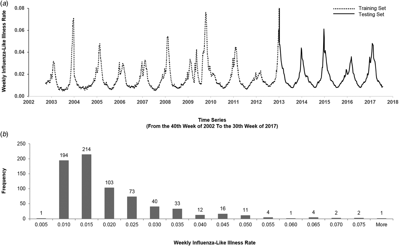
Figure 1(a) illustrates the historical plot of the US flu data. We split the duration into two parts: the first 2/3 (from the 40th week of 2002 to the 44th week of 2012) for training and the last 1/3 (from the 45th week of 2012 to the 30th week of 2017) for testing.

Fig. 1. The US flu data from the 40th week of 2002 to the 30th week of 2017. (a) We split the data into the training set and the testing set. The y-axis represents the weekly ILI rates, and the x-axis represents the time series (from the 40th week of 2002 to the 30th week of 2017). The dashed line is the first 2/3 of the data (from the 40th week of 2002 to the 52nd week of 2012) that were used for training, and the solid line is the last 1/3 of the data (from the first week of 2013 to the 30th week of 2017) that were used for testing. (b) The histogram of the weekly ILI rates of the US flu data. The y-axis represents the frequency, and the x-axis represents weekly ILI rates. The histogram is right-skewed.
Figure 1(b) describes the histogram of the weekly ILI rates. The histogram is right-skewed. Generally, comparing accuracy of models by mean absolute percentage error (MAPE) mainly reflects the difference of the ‘median’; while comparing by root mean square error primarily reflects the difference of the ‘mean’. The right-skewed histogram and the Kolmogorov–Smirnov test (P < 0.05) showed that the US flu data followed a non-normal distribution. Therefore, we expected that the accuracy would reflect the difference of ‘median’ and thereby used MAPE as a key performance indicator (KPI) for comparing models.
 $${\rm MAPE}\; = \; \displaystyle{1 \over n}\; \mathop \sum \limits_{t = 1}^n \; \; \left \vert {\displaystyle{{F_t - A_t} \over {A_t}}} \right \vert \; \times \; 100\%, $$
where A t is the actual value and F t is the forecast value.
Feature space and responses
For the feature space, we adopted the time lag of 52 weeks due to the result of one of our previous studies. In the previous study, we used the same US flu data and compared accuarcy of models of the different time lags of 2, 4, 9, 13, 26 and 52 weeks and found that of 52 weeks grew out the best accuracy [Reference Zhang and Nawata16]. Moreover, we calculated the first-order differences as a part of the feature spaces, since some past study found that first-order differences helped improve accuracy of the prediction models for flu data [Reference Wu18]. In brief, for feature spaces, we used (I) the ILI rate of the current week, (II) the ILI rates of the past 52 weeks and (III) the 52 first-order differences. Totally, we have 105 features.
Regarding responses, we were forecasting the two-, three-, four-, five-, six-, seven-, eight-, nine-, 10-, 11-, 12- and 13-step-ahead ILI rates.
Model
For multi-step prediction, there are mainly two types of methodologies: (I) ‘recursive’ prediction and (II) ‘jumping’ prediction. Generally, the methodology of (I) predicts values step-by-step; the methodology of (II) predicts some-step-ahead values independently. The following (a), (b), (c) and (d) explain four multi-step prediction algorithms [Reference Brownlee19].
(a) Multi-stage prediction (MSP)
MSP is a ‘recursive’ prediction. MSP uses one single-output model, which is recursively applied in multiple-step prediction, feeding through the previous output as its new input [Reference Cheng, Ng, Kitsuregawa, Li and Chang20]. In this study, as the first step, we predict X t+1 using the 53 historical values, i.e. X t, X t−1, X t−2, … and X t−52; as the second step, we predict X t+2 based on X t+1 (X t+1 was predicted in the first step), X t, X t−1, X t−2, … and X t−51; as the third step, we predict X t+3 based on X t+2 (X t+2 was predicted in the second step), X t+1 (X t+1 was predicted in the first step), X t, X t−1, X t−2, … and X t−50, etc. Formula 1 describes the prediction process.
Formula 1. Algorithm of MSP
prediction(t+1) = LSTM_MSP_MODEL#01(observation(t), observation(t−1), observation(t−2), …, observation(t−52))
prediction(t+2) = LSTM_MSP_MODEL#01(prediction(t+1), observation(t), observation(t−1), …, observation(t−51))
prediction(t+3) = LSTM_MSP_MODEL#01(prediction(t+2), prediction(t+1), observation(t), observation(t−1), …, observation (t−50))
…
prediction(t+13) = LSTM_MSP_MODEL#01(prediction (t+12), prediction(t+11), prediction(t+10), …, prediction(t+1), observation(t), observation(t−1), …, observation(t−40))
(b) Adjusted multi-stage prediction (AMSP)
AMSP is a refined version of MSP. Comparatively, when AMSP predicting X t+p (P ⩾ 2), it uses another model instead of using the same model repeatedly. Such a modification helps suppress error accumulation [Reference Venkatraman, Hebert and Bagnell21, Reference Akhlaghi and Zhou22]. Formula 2 illustrates the algorithm of AMSP.
Formula 2. Algorithm of AMSP
prediction(t+1) = LSTM_AMSP_MODEL#01(observation(t), observation(t−1), observation(t−2), …, observation(t−52))
prediction(t+2) = LSTM_AMSP_MODEL#02(prediction(t+1), observation(t), observation(t−1), …, observation(t−51))
prediction(t+3) = LSTM_MSP_MODEL#03(prediction(t+2), prediction(t+1), observation(t), observation(t−1), …, observation(t−50))
…
prediction(t+13) = LSTM_AMSP_MODEL#13(prediction(t+12), prediction(t+11), prediction(t+10), …, prediction(t+1), observation(t), observation(t−1), …, observation(t−40))
(c) Multiple single-output prediction (MSOP)
MSOP is a ‘jumping’ prediction. MSOP directly predicts a p-step-ahead (P ⩾ 2) value only by historical values: X t, X t−1, X t−2, …, X t–n. Formula 3 explains the algorithm of MSOP.
Formula 3. Algorithm of MSOP
prediction(t+1) = LSTM_MSOP_MODEL#01(observation(t), observation (t−1), observation(t−2), …, observation(t−52))
prediction(t+2) = LSTM_MSOP_MODEL#02(observation(t), observation(t−1), observation(t−2), …, observation(t−52))
prediction(t+3) = LSTM_MSOP_MODEL#03(observation(t), observation(t−1), observation(t−2), …, observation(t−52))
…
prediction(t+13) = LSTM_MSOP_MODEL#13(observation(t), observation(t−1), observation(t−2), …, observation(t−52))
(d) Multiple-output prediction (MOP)
MOP can be regarded as a merged version of MSOP. MOP uses one model to predict many some-step-ahead values all at once. In other fields, MOP was also implemented by multiple support vector regression [Reference Cheng, Ng, Kitsuregawa, Li and Chang20, Reference Zhang23, Reference Bao, Xiong and Hu24]. Formula 4 outlines the algorithm of MOP.
Formula 4. Algorithm of MOP
prediction(t+1), prediction(t+2), …, prediction(t+13) = LSTM_MOP_MODEL#01(observation(t), observation(t−1), observation(t−2), …, observation(t−52))
Coding
We used Python and Keras package (Version 2.0.4) [Reference Chollet25] based on Tensorflow (Version 1.1.0) [26]. We adopted an ‘early-stopping’ algorithm with a ‘patience’ of 100 epochs (for a total of 1000 epochs) and compared the predicting accuracy of LSTM models of the number of layers: 3–6 and 10.
Results
Results of MSP
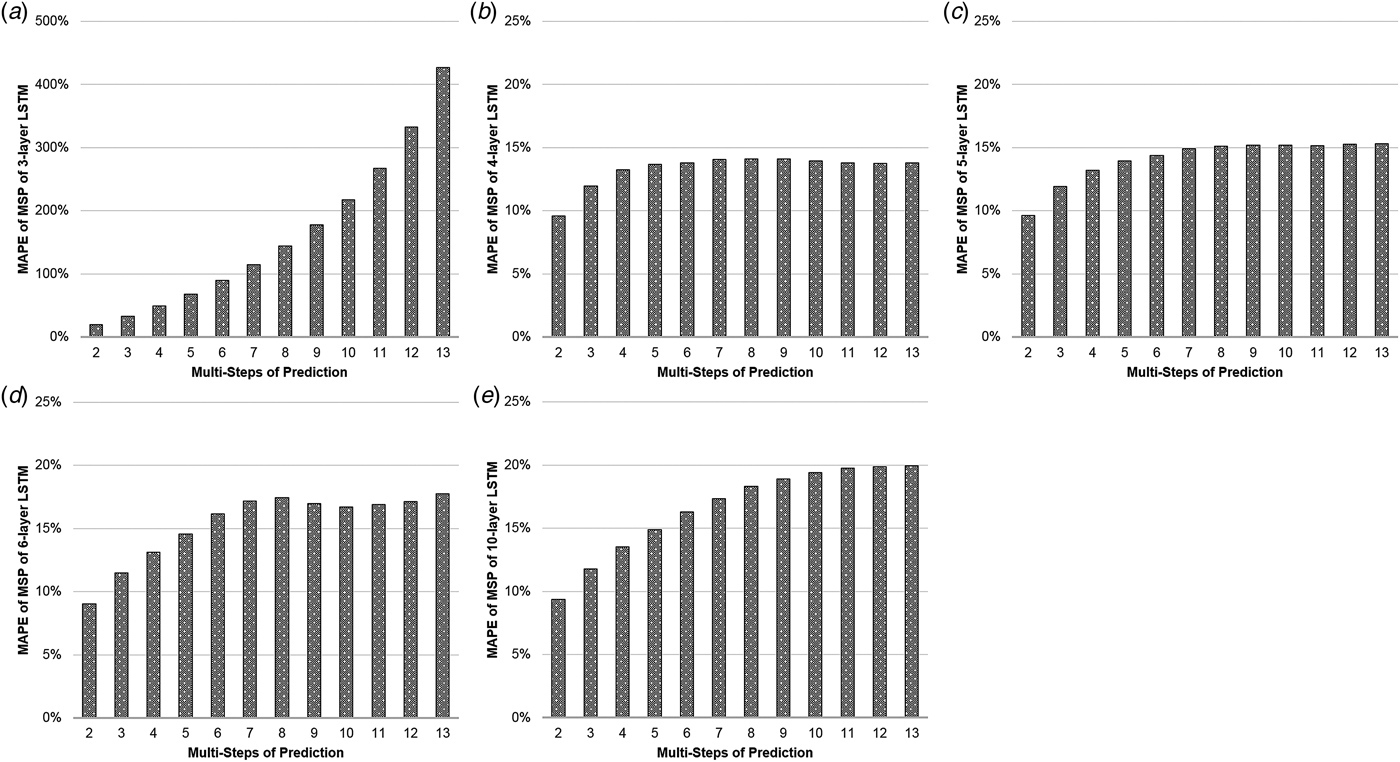
Table 1(a) illustrates the MAPEs of LSTM with MSP algorithm. The three-layer LSTM with MSP algorithm achieved the predicting MAPEs of 19.757, 32.969, 49.096, 67.866, 89.892, 114.977, 143.999, 177.719, 217.721, 267.335, 332.577 and 426.828%, when forecasting the ILI rates of the coming second to 13th weeks. The MAPE increased by nearly 22 times as the number of predicting steps increased. Comparatively, the MAPEs of the four-layer LSTM with MSP algorithm increased limitedly, from 9.57% to 13.77% with some slight setbacks in 10-, 11- and 12-step prediction. The similar phenomena occurred in the MAPEs of LSTM of five, six and 10 layers with MSP (Fig. 2).

Fig. 2. The MAPEs of LSTM with MSP. The y-axis represents the MAPE of the predictions and the x-axis represents multi-steps of the predictions. The (a–e) illustrate the MAPEs with the MSP algorithm of three-, four-, five-, six-, 10-layer LSTM, respectively.
Table 1. The MAPEs of LSTM with the multi-step predicting algorithms of MSP, AMSP, MSOP and MOP

MAPEs, mean absolute percentage errors; MSP, multi-stage prediction; LSTM, long short-term memory.

MAPEs, mean absolute percentage errors; AMSP, adjusted multi-stage prediction; LSTM, long short-term memory.

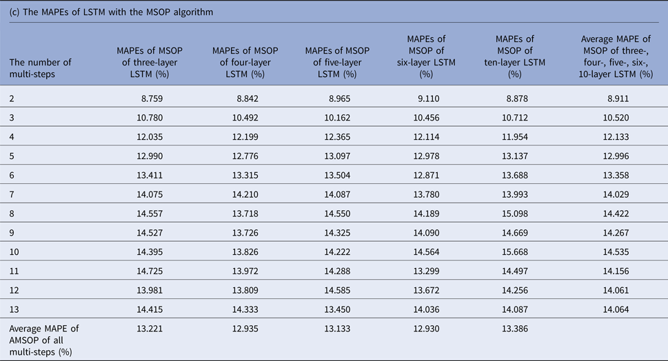
MAPEs, mean absolute percentage errors; MSOP, multiple single-output prediction; LSTM, long short-term memory.

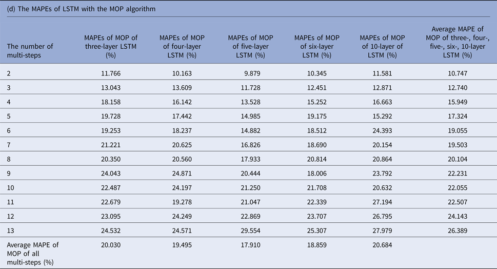
MAPEs, mean absolute percentage errors; MOP, multiple-output prediction; LSTM, long short-term memory.
Results of AMSP, MSOP and MOP
Tables 1(b–d) display the MAPEs of LSTM with AMSP, MSOP and MOP algorithm. In AMSP, the average MAPE increased from 9.171% to 14.715% as the number of predicting steps increased from two to 13, and varied from 13.626% to 13.911% as the number of layers of LSTM increased from three to 10 layers.
The average MAPEs of LSTM of both MSOP and MOP had a slight upward trend as the number of predicting steps increased (from 8.911% to 14.064% in MSOP; from 10.747% to 26.389% in MOP); and varied limitedly as the number of layers of LSTM increased (from 12.935% to 13.386% in MSOP; from 17.9100% to 20.684% in MOP).
In sharp contrast to MSP, the accuracy of AMSP, MSOP and MOP had little improvement when we used more layers of LSTM.
Comparison of the average MAPE of MSP, AMSP, MSOP and MOP
Figure 3 compares the average MAPEs of LSTM with multi-step predicting algorithms of MSP, AMSP, MSOP and MOP. The different numbers of the layers impacted the predicting accuracy tremendously in MSP (from 13.315% to 161.728%); slightly in MOP (from 17.910% to 20.684%), and barely in AMSP (from 13.626% to 13.911%) and MSOP (from 12.930% to 13.386%). Implementing MSOP in the six-layer LSTM structure achieved the best accuracy in this study. The MAPEs from two-step-ahead to 13-step-ahead prediction for the US ILI rates were all <15%, averagely 12.930%.

Fig. 3. The average MAPEs of LSTM with MSP, AMSP, MSOP and MOP. The y-axis represents the MAPE of the predictions and the x-axis represents the models of three-, four-, five-, six- and 10-layer LSTM with the multi-step predicting algorithms of MSP, AMSP, MSOP and MOP. Implementing MSOP in the six-layer LSTM achieved the lowest average MAPE of 12.930% in this study.
Discussion
Past studies
We did not find past studies that performed auto-regression in the multi-step prediction for flu outbreaks. Regarding multi-step prediction for studies in other fields, MSP is one of the most popular methodologies probably because many types of models can be used for this purpose, such as linear regression, support vector regression [Reference Muller, Gerstner, Germond, Hasler and Nicoud27], random forest, gradient boosting, artificial neural network [Reference Narendra and Parthasarathy28], etc. However, any such model inevitably introduces errors and tends to suffer from error accumulation problem when the predicted period is long. This is because the bias and variance from previous predictions impact future predictions [Reference Cheng, Ng, Kitsuregawa, Li and Chang20]. These compounding errors change the input distribution for future prediction steps, breaking the train-test independent and identically distributed assumption common in supervised learning [Reference Cheng, Ng, Kitsuregawa, Li and Chang20].
Comparison of accuracy of MSP, AMSP, MSOP and MOP
When comparing four different multi-step predicting algorithms, we found that the MAPEs of AMSP were less than those of MSP, which demonstrated AMSP suppressed the accumulated errors effectively based on its refined algorithm. Besides, the MAPEs of MSOP are less than those of MOP. As we mentioned in section ‘Methods’, to predict the ILI rates of the coming second to 13th weeks, MOP trained only one model while MSOP trained 13 models. As a result, MSOP can predict with no necessity of sharing neurons in LSTM structure, while MOP has to share neurons in LSTM structure. Consequently, the accuracy of MSOP performed better. Moreover, the average MAPEs of MSOP are slightly less than those of AMSP. The explanation is that MSOP does not accumulate errors at all, while AMSP just adjusted its accumulated errors by training new models. Therefore, MSOP performed best.
Other features
In our opinion, including other features in multi-step predicting models impacts models’ accuracy positively and negatively. For one thing, when predicting future values, other features could help predict more accurately, especially at turning points, such as an abrupt decrease in temperature. For another thing, before forecasting future ILI rates, we need to forecast other features (e.g. we need weather forecast for temperature and humidity). The error in former prediction could enlarge the error in later prediction. The mechanism is similar to MSP, which accumulates error step by step. In conclusion, whether the accuracy improves or deteriorates might depend on different data in different season from different countries.
In this study, we only performed auto-regression based on two pieces of consideration. First, we regard historical values as a response of all related features, such as temperature, humidity, etc. Therefore, to some extent, taking historical values as feature space includes all related features/factors in models. Besides, how to include temperature or humidity of the whole country in the models is a challenge work. Simply averaging temperature or humidity of all the places (cities and towns) of the USA might bring other problems, such as overlooking in population size, population density, life styles, etc. in different places.
Conclusion
In this study, we adjusted the LSTM model by the four multi-step prediction algorithms. The result showed that implementing MSOP in a six-layer LSTM structure achieved the best accuracy. The MAPEs from two-step-ahead to 13-step-ahead prediction for the US ILI rates were all <15%, averagely 12.930%. Hopefully, this accurate modelling approach will positively help hospitals, pharmaceutical companies, individuals and governments better prepare for the flu seasons and therefore prevent and control flu outbreaks worldwide.
Declaration of Interest
None.
Ethical Standards
The authors assert that all procedures contributing to this work comply with the ethical standards of the relevant national and institutional committees on human experimentation and with the Helsinki Declaration of 1975, as revised in 2008.


