I. INTRODUCTION
Nowadays, traditional power grids are facing many challenges, including load schedule uncertainties, low load factor, power transfers across different regions, and the incorporation of renewable energy systems. On the other hand, consumers are demanding better power quality and reliability, and the demand is arising due to the increase of new types of appliances such as plug-in hybrid electric vehicles. In such a case, efficient use and maintenance of current available resource to reduce environmental impacts becomes more and more important and has drawn great attention recently. It is evidently needed to transform traditional electric network using various smart devices, algorithms, and designs into a highly efficient and reliable power grid. A “Smart Grid” [Reference Farhangi1–4] is a future electricity delivery system based on new technologies, such as digital communication, computational algorithm, and market design. Such a power grid is expected to overlay the traditional electrical network with a smart metering system, which is capable of sensing and measuring power consumption from customers and applying two-way communications to improve the performance of power production, transmission, distribution, and consumption. The goals of smart grid are to enhance the reliability and quality of power supply, reduce the peak demand, improve the efficiency of the power grid, and lower the total energy consumption.
Demand response, one important feature of smart grid, is a mechanism that can motivate end-use customers to change their electricity usage from normal consumption patterns in response to the changes in the price of electricity over time [5–Reference Conejo, Morales and Baringo9]. By motivating end-use customers to reduce their electricity usage during critical peak periods or when system reliability is jeopardized, demand response has been shown to be able to make the power grid more efficient and reliable [Reference Severin, Jaske and Rosenfeld10–Reference Su and Kirschen14]. In the summer of 2003, the New York Independent System Operator (NYISO) paid out $ 7.2 million in incentive payments to over 1400 program participants for reducing peak load by 700 MW [15]. Such a load curtailment program brought reliability benefits of more than $ 50 million on August 15, 2003, which means that the benefits created by the load curtailment program exceeded the costs by a factor of 7:1. From customers' perspective, they expect savings in electricity bills by participating in the demand response program and reducing their electricity usages during peak periods. As reported in [Reference Braithwait and Eakin16], a small reduction of demand (5%) could have resulted in a 50% price reduction during the California electricity crisis in 2000–2001.
Generally, there are mainly two different categories of demand response algorithms [5, Reference Albadi and El-Saadany11]: incentive-based demand response and pricing-based demand response. In the incentive-based demand response, customers are given the incentive payments to reduce their consumptions in case of emergencies or when system reliability is jeopardized. For example, Chen et al. [Reference Chen, Li, Low and Doyle17] proposed to match the supply when the electricity supply is deficit based on supply function bidding. By shedding the load, customers can receive some revenue that is determined by the customers' supply functions. The authors then suggested an iterative and distributed supply function bidding scheme to achieve the market equilibrium that maximizes the social welfare. However, since customers' revenue is determined by all customers' supply functions, the bidding scheme is not incentive compatible, i.e., customers have the incentive to report false supply function to increase their revenue. In [Reference Faranda, Pievatolo and Tironi18], the authors proposed a distributed interruptible load shedding program to ensure the correct electrical system operation by increasing the number of participants. The optimal load reduction request is found by minimizing the expected value of an appropriate cost function which takes into account the uncertainty about the power absorbed by each customer. In [Reference Fahrioglu and Alvarado19], Fahrioglu and Alvarado designed an incentive compatible contract to encourage customers to reveal their true value of power interruptibility to achieve effective demand management. Since customers' values of power interruptibility keep changing over time and some customers may not be willing to disclose their private power interruptibility value, the contract-based approach in [Reference Fahrioglu and Alvarado19] cannot be directly applied to the real-time pricing demand response system.
In pricing-based demand response, due to the use of dynamic pricing, customers will dynamically adjust their consumption according to the time-varying price to maximize their payoffs. In [Reference Samadi, Mohsenian-Rad, Schober, Wong and Jatskevich20], the authors proposed a real-time pricing algorithm by maximizing the aggregate utility of all customers. Based on the dual decomposition, the authors then proposed a distributed implementation to automatically manage the interactions among the energy consumption controller units at the smart meters and the energy provider. With the presence of a real-time pricing tariff, Mohsenian–Rad and Leon–Garcia [Reference Mohsenian-Rad and Leon-Garcia21] proposed a residential energy consumption scheduling algorithm by considering the trade-off between the electricity payment and the waiting time for the operation of each appliance. Another type of pricing algorithm is the time-of-use pricing algorithm, where different unit prices are set for usage during different blocks of time, e.g., peak-load period, flat-load period, and valley-load period. In [Reference Zeng, Li and Ren22], the authors conducted a survey on the research of time-of-use electricity pricing models. To understand the effects of price responsive demand on whole sale and retail markets, Chao proposed an economic framework on pricing and investment [Reference po Chao23].
The importance of demand response can go far beyond reducing the electricity bills of customers. It facilitates the demand management from the operational perspective through real-time pricing to balance the demand and supply in the electric power market [Reference Barbose, Goldman and Neenan24, Reference Zhang, Fuller and Elhedhli25]. However, the additional dynamics and flexibility brought by demand response also increase the uncertainty and complexity of the centralized load forecast, which are critical issues of utilizing real-time pricing to regulate the total demand from customers. This uncertainty will pose new challenges and make the difficult centralized load forecast problem even harder, given the scale of today's power grid. In such a case, the forecast total demand from customers may not accurately reflect the future load. As a consequence, the power plant either overgenerates or undergenerates the power, which leads to low system efficiency and high risk of outage, respectively.
To overcome these challenges, we propose to use game theory to formulate the demand response problem. In this demand response game, the players are the power substation (or power plant) and the customers, where the objective of the power substation is to use real-time pricing to dynamically adjust the total demand to meet a target demand curve and the objective of the customers is to dynamically choose their optimal demands to maximize their own utilities. Recently, there have been some works using game theory for demand response. In [Reference Maharjan, Zhu, Zhang, Gjessing and Basar26], Maharjan et al. proposed to use Stackelberg game formulation to maximize the revenue of utility company and customers, whereas in [Reference Ibars, Navarro and Giupponi27] the authors proposed to use congestion game to control the power demand to achieve energy savings and utilization efficiency. However, neither the problem of enforcing truth-telling nor the problem of controlling the demand are investigated. In [Reference Mohsenian-Rad, Wong, Jatskevich, Schober and Leon-Garcia28], Mohsenian-Rad et al. proposed an autonomous and distributed demand-side energy management system by taking advantage of a two-way communication infrastructure among users. Different from [Reference Mohsenian-Rad, Wong, Jatskevich, Schober and Leon-Garcia28] that focused on the interactions among customers, in this paper, we focus on the interactions between power substation and customers.
The main contributions of this paper are summarized as follows.
-
(i) We propose a game-theoretic demand response scheme that can transform the traditional centralized load prediction structure into a distributed load prediction system by the participation of customers. Such a transformation would revolutionize the difficult and complex centralized forecasting into easy demand report collection.
-
(ii) Since the proposed scheme is distributed and customers are naturally selfish, enforcing truth-telling is crucial. We prove analytically and demonstrate with simulations that the proposed game-theoretic scheme is incentive compatible, i.e., all customers are motivated to report and consume their true optimal demands and any deviation will lead to a utility loss. Owing to the incentive compatible property of the proposed scheme, the aggregate demand report from the customers is an accurate estimate of the total consumption of customers. In such a case, the power substation can obtain an accurate estimate of the total consumption ahead of time and generate the corresponding amount of power, which can greatly improve the system efficiency and reduce the risk of outage.
-
(iii) We prove theoretically that the proposed demand response scheme can lead to the solution that is social welfare maximizing and proportionally fair in terms of the utility function.
-
(iv) To encourage participation, the demand response scheme should be simple since customers may not be willing to join the response scheme if the mechanism is complicated. The proposed demand response scheme is very simple. What customers need to do is to compute their own optimal demand for any given price and report the optimal demand to the power substation.
The rest of this paper is organized as follows. Section II introduces the game-theoretic formulation. In Section III, we describe in details the proposed incentive compatible mechanism and the dynamic pricing of the power substation. Then we show the simulation results to verify the proposed algorithm in Section IV. Finally, we draw conclusions in Section V.
II. GAME-THEORETIC FORMULATION
We consider a smart grid with N customers that are served by one power substation as shown in Fig. 1. Customers are assumed to be intelligent and can make optimal decision based on the price of the power. Such customers can be residential customers who are equipped with smart meters that can automatically predict and adjust the electricity usage, or “big” customers such as commercial buildings and industrial participants who have dedicated facility personnel to manage electricity usage. On the other hand, the power substation is assumed to have a target total demand curve. The objective of the power substation is to control the total demand of all customers to meet the target demand curve by dynamically adjusting the unit price of the power. The problem is to determine how the power substation should use dynamic pricing to control the total demand.
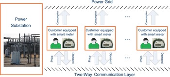
Fig. 1. System model.
One possible approach for the power substation to achieve this task is the centralized approach where the power substation predicts the total demand of all customers by estimating the behavior of the customers using power consumption history. For example, the power substation can first find the time slot with the most similar conditions by searching over the power consumption history, and then predict the total demand using the actual total power consumption at that time slot. However, this kind of centralized approach has several drawbacks. First, the computational complexity at the power substation is very high since the power substation needs to estimate the behaviors of all customers and predict their power consumption. Second, the prediction accuracy of the total demand consumption may not be high due to the complex behavior of customers. Third, due to the inaccurate prediction, the power substation may overgenerate or undergenerate power which leads to power inefficiency or power outage.
To overcome these drawbacks, we propose a game-theoretic demand response scheme to transform the traditional centralized load prediction structure into a distributed load prediction system by the participation of customers, i.e., we ask the customers to report their demands to the power substation. Since customers, especially the “big” customers such as commercial buildings and industrial participants, are rational and thus naturally selfish, they tend to overclaim what they may need and will not truly report their optimal demand if cheating can improve their payoffs. To motivate customers to report their true optimal demands, we propose an incentive compatible mechanism by carefully designing the penalty function for deviation. Formally, the demand response game can be defined as follows:
-
• Players: The players are the N rational customers and the power substation.
-
• Strategies: The strategies of customer i is $\lpar \hat{d}_{i}\comma \; d_{i}\rpar $
, where $\hat{d}_{i}$
is the demand that customer i reports to the power substation and d
i
is the real demand that customer i consumes. The strategies of the power station is $\lpar p_{i}\comma \; C_{i}\lpar p^{r}\comma \; d_{i}\comma \; \hat{d}_{i}\rpar \rpar $
, where p
i
is the real-time price announced to customer i and $C_{i}\lpar p_{i}\comma \; d_{i}\comma \; \hat{d}_{i}\rpar $
is the cost function that the power station will use to charge customer i who takes strategies $\lpar \hat{d}_{i}\comma \; d_{i}\rpar $
.
 -
• Utility function: By taking strategies $\lpar \hat{d}_{i}\comma \; d_{i}\rpar $
, the utility function of customer i can be formally written as
(1)where G i (d i ) is the gain function customer i receives by consuming d i ,
 $$U_i\lpar d_i\comma \; \hat{d}_i\rpar = \lambda G_i\lpar d_i\rpar - C_i\lpar p_i\comma \; d_i\comma \; \hat{d}_i\rpar \comma \;$$ $C_{i}\lpar p_{i}\comma \; d_{i}\comma \; \hat{d}_{i}\rpar $
is the cost customer i needs to pay to the power substation, and λ is a parameter balancing the gain and the cost, which is assumed to be the same for all customers. The details of the gain and cost function will be introduced in the next section. On the other hand, the objective of the power substation is to use real-time pricing, i.e., p
i
′s, to dynamically adjust the total demand to meet a certain target demand. Instead of specifying the utility function of power substation here, we will discuss how the power substation determines p
i
′s in the next section.
III. ANALYSIS OF THE DEMAND RESPONSE GAME
A) Gain function of the customer
Generally, by consuming a certain amount of power, a customer experiences a certain gain which reflects the level of satisfaction. For example, when reading under a bad lighting condition, a customer will feel happy by turning on a light, and such a happiness can be characterized by a certain gain. We assume that each customer i has a minimal power demand d i min to operate some essential appliances such as refrigerator and air conditioner. If the demand is smaller than d i min, the customer will feel very uncomfortable, so the gain is zero. Once the power demand reaches d i min, the customer experiences a gain g i . After satisfying the minimal demand constraint, the gain will increase by a certain value if an additional appliance is turned on. Since customers are intelligent and rational, they will always first turn on the appliance that can bring the largest increase of their level of satisfaction. For example, a customer in a dark room will turn on the light first, whereas the customer who feels hot will turn on the fan first. With such an intuition, the gain function should be an increasing step function with the step size decreasing over the demand for all demand that is larger than the minimal demand constraint, e.g., the red dot curve in Fig. 2. Since the gain function characterizes the level of satisfaction of the customer, it can be different under different climate conditions and different moods of the customer. For example, the pink dash curve and blue dot-dash curve in Fig. 2 can be the gain functions under two different conditions. To better understand the behavior of the customers, we assume that the gain function measures the average level of satisfaction under different conditions such as climate and mood conditions.
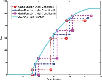
Fig. 2. An illustration of the gain function. The red, blue, and pink dot-dash curves stand for the gain functions under different climate conditions and different moods of the customer, whereas the cyan curve is the gain function that measures the average level of satisfaction under different conditions.
From the above discussion, we can see that the gain should be zero for any demand smaller than the minimal demand constraint. For the demand larger than the minimal demand constraint, the gain function should be a monotonically increasing concave function with the level of satisfaction gradually saturating. After the demand reaching the maximal demand constraint which can be the total power demand for operating all appliances, the gain function should remain constant. There are many possible gain functions. In this paper, we use a modified quadratic gain function G i (d) defined in (2) and illustrated as the cyan solid curve in Fig. 2. A similar gain function was used in [Reference Samadi, Mohsenian-Rad, Schober, Wong and Jatskevich20]. Note that our scheme can be easily extended to other gain functions.
 $$G_i\lpar d\rpar = \left\{\matrix{0\comma \; \hfill &\hbox{if} 0 \leq d \lt d_i^{\min}\semicolon \; \hfill \cr - {\alpha_i \over 2} \lpar d - d_i^{\min}\rpar ^2 \hfill \cr \quad + w_i\lpar d-d_i^{\min}\rpar + g_i\comma \; \hfill &\hbox{if } d_i^{\min} \leq d \leq {w_i \over \alpha_i} \hfill \cr {} & \quad+ d_i^{\min}\semicolon \; \hfill \cr {w_i^2 \over 2\alpha_i} + g_i\comma \; \hfill &\hbox{if } d \gt {w_i \over \alpha_i} + d_i^{\min}\comma \; \hfill} \right.$$
where d i min is the minimal power demand, g i is the gain of the minimal power demand, α i is the parameter controlling the speed of increase of the quadratic function which can be time-varying, and w i is the declivity of the parabola at d = d i min which is fixed over time.
B) The proposed mechanism for power substation
To motivate customers to report their true optimal demands to power substation, we propose an incentive compatible mechanism as follows. At the beginning of time slot t, the power substation announces a reference price p
r
to all customers. How to determine the reference price p
r
will be discuss in Section III-F. After receiving the reference price, each customer computes the optimal demand
![]() $d_{i}^{\star}$
by maximizing the intermediate utility function as follows:
$d_{i}^{\star}$
by maximizing the intermediate utility function as follows:
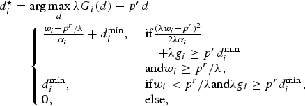 $$\eqalign{d_i^{\star} &= \arg \max_{d} \lambda G_i\lpar d\rpar - p^r d \cr &= \left\{\matrix{{w_i-p^r/\lambda \over \alpha_i} + d_i^{\min}\comma \; \hfill &\hbox{if} {\lpar \lambda w_i - p^r\rpar ^2 \over 2\lambda \alpha_i} \hfill \cr {} \hfill &\quad + \lambda g_i \geq p^r d_i^{\min} \hfill \cr {} \hfill &\hbox{and} w_i \geq p^r/\lambda\comma \; \hfill \cr d_i^{\min}\comma \; \hfill &\hbox{if} w_i \lt p^r/\lambda \hbox{and} \lambda g_i \geq p^r d_i^{\min}\comma \; \hfill \cr 0\comma \; \hfill &\hbox{else}\comma \; \hfill} \right.}$$
Nevertheless, we should notice that customers may not report their true optimal demand
![]() $d_{i}^{\star}$
to the power substation due to their selfish nature. Let us assume that customer i reports
$d_{i}^{\star}$
to the power substation due to their selfish nature. Let us assume that customer i reports
![]() $\hat{d}_{i}$
to the power substation. After receiving all the demands from the customers, the power substation announces to each customer i the cost function
$\hat{d}_{i}$
to the power substation. After receiving all the demands from the customers, the power substation announces to each customer i the cost function
![]() $C_{i}\lpar p_{i}\comma \; d_{i}\comma \; \hat{d}_{i}\rpar $
as follows
$C_{i}\lpar p_{i}\comma \; d_{i}\comma \; \hat{d}_{i}\rpar $
as follows
where p i is defined as
and m is a constant which can be treated as the maintenance fee,
![]() $\Delta \geq \max \lcub w_{1}\comma \; \ldots\comma \; w_{N}\rcub $
and
$\Delta \geq \max \lcub w_{1}\comma \; \ldots\comma \; w_{N}\rcub $
and
![]() $\rho \geq \max\lcub g_{1}\comma \; \ldots\comma \; g_{N}\rcub $
are two fixed parameters. From (4), we can see that customers are punished for both overreporting and underreporting. For overreporting, customers will be charged for what they reported, which can be treated as a pre-paid rule. For underreporting, customers will receive a penalty that is linear in the deviation
$\rho \geq \max\lcub g_{1}\comma \; \ldots\comma \; g_{N}\rcub $
are two fixed parameters. From (4), we can see that customers are punished for both overreporting and underreporting. For overreporting, customers will be charged for what they reported, which can be treated as a pre-paid rule. For underreporting, customers will receive a penalty that is linear in the deviation
![]() $d_i - \hat{d}_{i}$
.
$d_i - \hat{d}_{i}$
.
Finally, according to the price p
i
, each customer consumes power d
i
and pays
![]() $C_{i}\lpar p_{i}\comma \; d_{i}\comma \; \hat{d}_{i}\rpar $
, and the utility function of customer i can be computed as in (1).
$C_{i}\lpar p_{i}\comma \; d_{i}\comma \; \hat{d}_{i}\rpar $
, and the utility function of customer i can be computed as in (1).
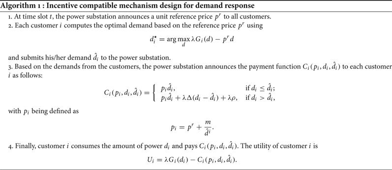
The detailed interactions between the power substation and customers are summarized in Algorithm 1 In the next three subsections, we will prove that the proposed demand response mechanism is incentive compatible and the outcome of the proposed demand response mechanism maximizes the social welfare, which is the sum of the customers' utilities and the revenue of the substation, and is proportionally fair in terms of the utility function.
Algorithm 1: Incentive compatible mechanism design for demand response
C) Incentive compatible property
In this subsection, we prove that the proposed mechanism is incentive compatible, which means that all customers are motivated to report and consume the optimal demands, i.e., their utility is maximized when
![]() $d_{i}=\hat{d}_{i}=d_{i}^{\star}$
, and any deviation will lead to a utility loss.
$d_{i}=\hat{d}_{i}=d_{i}^{\star}$
, and any deviation will lead to a utility loss.
Lemma 1
After reporting
![]() $\hat{d}_{i}$
, the best strategy of customer i at the consumption stage is to consume
$\hat{d}_{i}$
, the best strategy of customer i at the consumption stage is to consume
![]() $\hat{d}_{i}$
, i.e.,
$\hat{d}_{i}$
, i.e.,
![]() $U_{i}\lpar d_{i}\comma \; \hat{d}_{i}\rpar \leq U_{i}\lpar \hat{d}_{i}\comma \; \hat{d}_{i}\rpar \comma \; \forall d_{i}$
, with equality if and only if
$U_{i}\lpar d_{i}\comma \; \hat{d}_{i}\rpar \leq U_{i}\lpar \hat{d}_{i}\comma \; \hat{d}_{i}\rpar \comma \; \forall d_{i}$
, with equality if and only if
![]() $d_i = \hat{d}_{i}$
.
$d_i = \hat{d}_{i}$
.
Proof: To prove
Lemma 1
, we need to show that
![]() $U_{i} \lpar d_{i}\comma \; \hat{d}_{i}\rpar - U_{i}\lpar \hat{d}_{i}\comma \; \hat{d}_{i}\rpar \leq 0\comma \; \forall d_{i}$
, with equality if and only if
$U_{i} \lpar d_{i}\comma \; \hat{d}_{i}\rpar - U_{i}\lpar \hat{d}_{i}\comma \; \hat{d}_{i}\rpar \leq 0\comma \; \forall d_{i}$
, with equality if and only if
![]() $d_i = \hat{d}_{i}$
. Since the payment function
$d_i = \hat{d}_{i}$
. Since the payment function
![]() $C_{i}\lpar p_{i}\comma \; d_{i}\comma \; \hat{d}_{i}\rpar $
in (4) is a piecewise function of d
i
, we will compute the difference between
$C_{i}\lpar p_{i}\comma \; d_{i}\comma \; \hat{d}_{i}\rpar $
in (4) is a piecewise function of d
i
, we will compute the difference between
![]() $U_{i}\lpar d_{i}\comma \; \hat{d}_{i}\rpar $
and
$U_{i}\lpar d_{i}\comma \; \hat{d}_{i}\rpar $
and
![]() $U_{i}\lpar \hat{d}_{i}\comma \; \hat{d}_{i}\rpar $
for each region.
$U_{i}\lpar \hat{d}_{i}\comma \; \hat{d}_{i}\rpar $
for each region.
-
• If $d_{i} \leq \hat{d}_{i}$
, according to (2), (4), and (1), we have
(6)where the last inequality comes from the monotonically increasing property of G i (.) function, and the equality holds if and only if
 $$\eqalign{&U_i\lpar d_i\comma \; \hat{d}_i\rpar - U_i\lpar \hat{d}_i\comma \; \hat{d}_i\rpar \cr &\quad = \lambda G_i\lpar d_i\rpar - C_i\lpar p_i\comma \; d_i\comma \; \ hat{d}_i\rpar \cr &\qquad - \left[\lambda G_i\lpar \hat{d}_i\rpar - C_i\lpar p_i\comma \; \hat{d}_i\comma \; \hat{d}_i\rpar \right]\cr &\quad = \lambda \left[G_i\lpar d_i\rpar - G_i\lpar \hat{d}_i\rpar \right]\cr &\quad \leq 0\comma \; }$$ $d_{i} = \hat{d}_{i}$
.
-
• Similarly, if $d_{i} \gt \hat{d}_{i}$
, from (2), (4), and (1), we have
(7)where the first inequality comes from the definitions of Δ and ρ that Δ≥ max {w 1, …, w N } and ρ≥ max {g 1, …, g N }.
 $$\eqalign{& U_i\lpar d_i\comma \; \hat{d}_i\rpar - U_i\lpar \hat{d}_i\comma \; \hat{d}_i\rpar \cr &\quad = \lambda G_i\lpar d_i\rpar -C_i\lpar p_i\comma \; d_i\comma \; \hat{d}_i\rpar \cr &\qquad -\left[\lambda G_i\lpar \hat{d}_i\rpar - C_i\lpar p_i\comma \; \hat{d}_i\comma \; \hat{d}_i\rpar \right]\cr &\quad = \lambda G_i\lpar d_i\rpar - \lambda G_i \lpar \hat{d}_i\rpar - \lambda \Delta \lpar d_i - \hat{d}_i\rpar - \lambda \rho \cr &\quad \leq \lambda \left[G_i\lpar d_i\rpar - G_i \lpar \hat{d}_i\rpar - w_i\lpar d_i - \hat{d}_i\rpar - g_i \right]\cr &\quad = \lambda \left\{\matrix{-w_i\lpar d_i-\hat{d}_i\rpar -g_i \lt 0\comma \; \hfill \cr \quad \hbox{if } 0 \leq \hat{d}_i \lt d_i \lt d_i^{\min}\semicolon \; \hfill \cr -{\alpha_i \over 2}\lpar d_i - d_i^{\min}\rpar ^2 + w_i\lpar \hat{d}_i - d_i^{\min}\rpar \lt 0\comma \; \hfill \cr \quad \hbox{if } 0 \leq \hat{d}_i \lt d_i^{\min} \leq d_i \leq {w_i \over \alpha_i} + d_i^{\min}\semicolon \; \hfill \cr -w_i\left(d_i - \hat{d}_i - {w_i \over 2\alpha_i} \right)\lt 0\comma \; \hfill \cr \quad \hbox{if } 0 \leq \hat{d}_i \lt d_i^{\min} \leq {w_i \over \alpha_i} + d_i^{\min} \lt d_i\semicolon \; \hfill \cr -{\alpha_i \over 2} \lpar d_i - \hat{d}_i\rpar \lpar d_i + \hat{d}_i - 2d_i^{\min}\rpar - g_i \lt 0\comma \; \hfill \cr \quad \hbox{if } d_i^{\min} \leq \hat{d}_i \lt d_i \leq {w_i \over \alpha_i} + d_i^{\min}\semicolon \; \hfill \cr -w_i\lpar d_i - d_i^{\min}\rpar + {w_i^2 \over 2\alpha_i} + {\alpha_i \over 2}\lpar \hat{d}_i - d_i^{\min}\rpar ^2 \hfill \cr \quad - g_i \lt 0\comma \; \hfill \cr \quad \hbox{if } d_i^{\min}\leq \hat{d}_i \leq {w_i \over \alpha_i} + d_i^{\min} \lt d_i\semicolon \; \hfill \cr - w_i\lpar d_i - \hat{d}_i\rpar - g_ i \lt 0\comma \; \hfill \cr \quad \hbox{if } {w_i \over \alpha_i} + d_i^{\min} \lt \hat{d}_i \lt d_i. \hfill} \right. \cr &\quad \lt 0\comma \; }$$
In all, according to (6) and (7), we can show that
![]() $U_{i}\lpar d_{i}\comma \; \hat{d}_{i}\rpar \leq U_{i} \lpar \hat{d}_{i}\comma \; \hat{d}_{i}\rpar \comma \; \forall d_{i}$
, with equality if and only if
$U_{i}\lpar d_{i}\comma \; \hat{d}_{i}\rpar \leq U_{i} \lpar \hat{d}_{i}\comma \; \hat{d}_{i}\rpar \comma \; \forall d_{i}$
, with equality if and only if
![]() $d_{i} = \hat{d}_{i}$
. Therefore, after reporting
$d_{i} = \hat{d}_{i}$
. Therefore, after reporting
![]() $\hat{d}_{i}$
, the best strategy of customer i at the consumption stage is to consume
$\hat{d}_{i}$
, the best strategy of customer i at the consumption stage is to consume
![]() $\hat{d}_{i}$
. □
$\hat{d}_{i}$
. □
Theorem 1
The proposed mechanism is incentive compatible.
Proof: To prove
Theorem 1
, we need to show that the utility of the customer is maximized when he/she reports and consumes the optimal demand, i.e.,
![]() $U_{i}\lpar d_{i}\comma \; \hat{d}_{i}\rpar $
is maximized at
$U_{i}\lpar d_{i}\comma \; \hat{d}_{i}\rpar $
is maximized at
![]() $d_{i}=\hat{d}_{i}=d_{i}^{\star}$
. According to (3), (5), (4), (1), and
Lemma 1
, we have
$d_{i}=\hat{d}_{i}=d_{i}^{\star}$
. According to (3), (5), (4), (1), and
Lemma 1
, we have
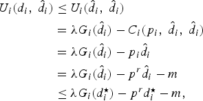 $$\eqalign{U_i\lpar d_i\comma \; \hat{d}_i\rpar &\leq U_i\lpar \hat{d}_i\comma \; \hat{d}_i\rpar \cr & = \lambda G_i\lpar \hat{d}_i\rpar - C_i \lpar p_i\comma \; \hat{d}_i\comma \; \hat{d}_i\rpar \cr &= \lambda G_i \lpar \hat{d}_i\rpar - p_i \hat{d}_i \cr &= \lambda G_i \lpar \hat{d}_i\rpar - p^r \hat{d}_i - m \cr &\leq \lambda G_i\lpar d_i^{\star}\rpar - p^r d_i^{\star} - m\comma \; }$$
where the first inequality is the consequence of
Lemma 1
; The three equalities come from the definition of utility function shown in (1), the definition of payment function shown in (4), and the definition of price function shown in (5), respectively. The last inequality comes from the definition of
![]() $d_{i}^{\star}$
shown in (3).
$d_{i}^{\star}$
shown in (3).
Note that equality in (8) holds if and only if
![]() $d_{i}=\hat{d}_{i}=d_{i}^{\star}$
. Therefore, all customers will try to report and consume the optimal demand to achieve maximal utility, and any deviation will lead to a utility loss, i.e., the proposed mechanism is incentive compatible. □
$d_{i}=\hat{d}_{i}=d_{i}^{\star}$
. Therefore, all customers will try to report and consume the optimal demand to achieve maximal utility, and any deviation will lead to a utility loss, i.e., the proposed mechanism is incentive compatible. □
D) Maximizing social welfare
In this subsection, we prove that the proposed mechanism leads to an equilibrium that maximizes the social welfare, which is the sum of the customers' utilities and the revenue of the substation.
Theorem 2
The proposed mechanism maximizes the social welfare, i.e.
![]() $\lpar d_{1}^{\star}\comma \; d_{2}^{\star}\comma \; \ldots\comma \; d_{N}^{\star}\rpar $
is the solution to the following optimization problem:
$\lpar d_{1}^{\star}\comma \; d_{2}^{\star}\comma \; \ldots\comma \; d_{N}^{\star}\rpar $
is the solution to the following optimization problem:
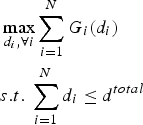 $$\eqalign{&\max_{d_i\comma \forall i} \sum_{i=1}^N G_i\lpar d_i\rpar \cr & s.t.\ \sum_{i=1}^N d_i \leq d^{total}}$$
with $d^{total} = \sum_{i=1}^{N} d_{i}^{\star}$
.
Proof: We will prove the theorem using contradiction. Suppose there exists a solution
![]() $\lpar \hat{d}_{1}\comma \; \hat{d}_{2}\comma \; \ldots\comma \; \hat{d}_{N}\rpar $
that satisfies the constraint
$\lpar \hat{d}_{1}\comma \; \hat{d}_{2}\comma \; \ldots\comma \; \hat{d}_{N}\rpar $
that satisfies the constraint $\sum_{i=1}^{N} \hat{d}_{i}\leq d^{total}$
and can lead to a larger social welfare than
![]() $\lpar d_{1}^{\star}\comma \; d_{2}^{\star}\comma \; \ldots\comma \; d_{N}^{\star}\rpar $
, i.e.,
$\lpar d_{1}^{\star}\comma \; d_{2}^{\star}\comma \; \ldots\comma \; d_{N}^{\star}\rpar $
, i.e.,
 $$\sum_{i = 1}^N G_i\lpar \hat{d}_i\rpar \gt \sum_{i = 1}^N G_i\lpar d_i^{\star}\rpar.$$
Then, since $\sum_{i=1}^{N} \hat{d}_{i}\leq d^{total}=\sum_{i=1}^{N} d_{i}^{\star}$
, we have
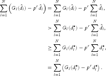 $$\eqalign{\sum_{i = 1}^N \left(G_i\lpar \hat{d}_i\rpar - p^r \hat{d}_i \right)&= \sum_{i = 1}^N G_i\lpar \hat{d}_i\rpar - p^r \sum_{i = 1}^N \hat{d}_i\comma \; \cr &\gt \sum_{i = 1}^N G_i \lpar d_i^{\star}\rpar - p^r \sum_{i = 1}^N \hat{d}_i\comma \; \cr &\geq \sum_{i = 1}^N G_i\lpar d_i^{\star}\rpar - p^r \sum_{i = 1}^N d_i^{\star}\comma \; \cr &= \sum_{i = 1}^N \left(G_i\lpar d_i^{\star}\rpar - p^r d_i^{\star} \right).}$$
According to (11), there is at least one
![]() $\hat{d}_{i}$
such that
$\hat{d}_{i}$
such that
![]() $G_{i}\lpar \hat{d}_{i}\rpar - p^{r}\hat{d}_{i} \gt G_{i}\lpar d_{i}^{\star}\rpar - p^{r}d_{i}^{\star}$
. This contradicts with the definition of
$G_{i}\lpar \hat{d}_{i}\rpar - p^{r}\hat{d}_{i} \gt G_{i}\lpar d_{i}^{\star}\rpar - p^{r}d_{i}^{\star}$
. This contradicts with the definition of
![]() $d_{i}^{\star}$
in (3). Therefore,
$d_{i}^{\star}$
in (3). Therefore,
![]() $\lpar d_{1}^{\star}\comma \; d_{2}^{\star}\comma \; \ldots\comma \; d_{N}^{\star}\rpar $
is the solution to the optimization problem in (9) that maximizes the social welfare. □
$\lpar d_{1}^{\star}\comma \; d_{2}^{\star}\comma \; \ldots\comma \; d_{N}^{\star}\rpar $
is the solution to the optimization problem in (9) that maximizes the social welfare. □
E) Proportionally fair solution
In this subsection, we prove that the proposed mechanism leads to the solution that is proportionally fair in terms of utility. Proportional fairness is the generalization of the Nash bargaining solution for multiple users [Reference Kelly29, Reference Han, Ji and Liu30]. Under the Nash bargaining, a transfer of resources between two users is favorable and fair if the percentage increase in the utility of one player is larger than the percentage decrease in utility of the other user. Under proportional fairness, the fair allocation should be such that, if compared to any other feasible allocation of utilities, the aggregate proportional change is less than or equal to zero. A formal definition of proportional fairness is given as follows.
Definition 1
A utility distribution is said to be proportionally fair when any change in the distribution of utilities results in the sum of the proportional changes being non-positive, i.e.,
 $$\sum_i {U_i - \tilde{U}_i \over \tilde{U}_i} \leq 0\comma \; \quad \forall U_i \in {\bf S}\comma \;$$
where Ũ i and U i are the proportionally fair utility and any other feasible utility for the ith user, respectively, and S is a closed and convex subset of ℜ N to represent the set of feasible utility functions that the users can achieve.
Remark 1
The definition of proportional fairness comes from the fact that, if
![]() $\lpar \tilde{U}_{1}\comma \; \tilde{U}_{2}\comma \; \ldots\comma \; \tilde{U}_{N}\rpar $
satisfied (12), any deviation from
$\lpar \tilde{U}_{1}\comma \; \tilde{U}_{2}\comma \; \ldots\comma \; \tilde{U}_{N}\rpar $
satisfied (12), any deviation from
![]() $\lpar \tilde{U}_{1}\comma \; \tilde{U}_{2}\comma \; \ldots\comma \; \tilde{U}_{N}\rpar $
will lead to a non-increasing sum of the proportional changes. Moreover, from [Reference Kelly29, Reference Han, Ji and Liu30], we can see that
$\lpar \tilde{U}_{1}\comma \; \tilde{U}_{2}\comma \; \ldots\comma \; \tilde{U}_{N}\rpar $
will lead to a non-increasing sum of the proportional changes. Moreover, from [Reference Kelly29, Reference Han, Ji and Liu30], we can see that
![]() $\lpar \tilde{U}_{1}\comma \; \tilde{U}_{2}\comma \; \ldots\comma \; \tilde{U}_{N}\rpar $
is a proportionally fair utility if and only if
$\lpar \tilde{U}_{1}\comma \; \tilde{U}_{2}\comma \; \ldots\comma \; \tilde{U}_{N}\rpar $
is a proportionally fair utility if and only if $\prod_{i=1}^{N} \tilde{U}_{i} \geq \prod_{i = 1}^{N} U_{i}$
for any feasible
![]() $\lpar U_{1}\comma \; U_{2}\comma \; \ldots\comma \; U_{N}\rpar $
.
$\lpar U_{1}\comma \; U_{2}\comma \; \ldots\comma \; U_{N}\rpar $
.
Theorem 3
The proposed mechanism leads to the solution that is proportionally fair in terms of utility, i.e.
![]() $\lpar d_{1}^{\star}\comma \; d_{2}^{\star}\comma \; \ldots\comma \; d_{N}^{\star}\rpar $
is the solution to the following optimization problem:
$\lpar d_{1}^{\star}\comma \; d_{2}^{\star}\comma \; \ldots\comma \; d_{N}^{\star}\rpar $
is the solution to the following optimization problem:
 $$\max_{d_i\comma \forall i} \prod_{i = 1}^N \left(G_i\lpar d_i\rpar - p^rd_i \right).$$
Proof: We will prove the theorem using contradiction. Suppose there exists a solution
![]() $\lpar \hat{d}_{1}\comma \; \hat{d}_{2}\comma \; \ldots\comma \; \hat{d}_{N}\rpar $
that can lead to a larger product of utility than
$\lpar \hat{d}_{1}\comma \; \hat{d}_{2}\comma \; \ldots\comma \; \hat{d}_{N}\rpar $
that can lead to a larger product of utility than
![]() $\lpar d_{1}^{\star}\comma \; d_{2}^{\star}\comma \; \ldots\comma \; d_{N}^{\star}\rpar $
, i.e.,
$\lpar d_{1}^{\star}\comma \; d_{2}^{\star}\comma \; \ldots\comma \; d_{N}^{\star}\rpar $
, i.e.,
 $$\prod_{i=1}^N \left(G_i\lpar \hat{d}_i\rpar - p^r\hat{d}_i\right)\gt \prod_{i = 1}^N \left(G_i\lpar d_i^{\star}\rpar - p^rd_i^{\star}\right).$$
In such a case, there is at least one
![]() $\hat{d}_{i}$
such that
$\hat{d}_{i}$
such that
![]() $G_{i}\lpar \hat{d}_{i}\rpar -p^{r}\hat{d}_{i}>G_{i}\lpar d_{i}^{\star}\rpar -p^{r}d_{i}^{\star}$
. This contradicts with the definition of
$G_{i}\lpar \hat{d}_{i}\rpar -p^{r}\hat{d}_{i}>G_{i}\lpar d_{i}^{\star}\rpar -p^{r}d_{i}^{\star}$
. This contradicts with the definition of
![]() $d_{i}^{\star}$
in (3). Therefore,
$d_{i}^{\star}$
in (3). Therefore,
![]() $\lpar d_{1}^{\star}\comma \; d_{2}^{\star}\comma \; \ldots\comma \; d_{N}^{\star}\rpar $
is proportionally fair in terms of utility. □
$\lpar d_{1}^{\star}\comma \; d_{2}^{\star}\comma \; \ldots\comma \; d_{N}^{\star}\rpar $
is proportionally fair in terms of utility. □
F) Dynamic pricing of the power substation
From the above discussion, we can see that the proposed mechanism is incentive compatible and can lead to the solution that is proportionally fair and social welfare maximizing, due to which all rational customers are motivated to report and consume the optimal demand. In such a case, according to (3), the average power consumption of the customers at time slot t can be computed as follows:
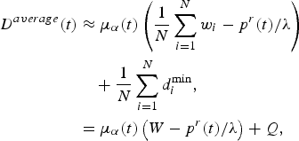
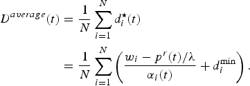 $$\eqalign{D^{average} \lpar t\rpar & = {1 \over N} \sum_{i = 1}^N d_i^{\star} \lpar t\rpar \cr & = {1 \over N} \sum_{i = 1}^N \left({w_i - p^r\lpar t\rpar /\lambda \over \alpha_i \lpar t\rpar } + d_i^{\min} \right).}$$
Here, we exclude the inactive customers whose optimal demand is zero and simply assume N is the total number of active customers. Moreover, we assume that the parameters w i and d i min are time-invariant parameters, whereas the parameter α i (t) is a time-variant parameter.
As discussed in Section III-A, α
i
(t) is the parameter controlling the speed of increase of the quadratic gain function. According to (15), if
![]() ${1 \over \alpha_{i}\lpar t\rpar }$
is modeled as a Gaussian distribution with mean μα(t) and constant variance σα
2, then, with the law of large numbers, the average power consumption of all customers can be approximated as
${1 \over \alpha_{i}\lpar t\rpar }$
is modeled as a Gaussian distribution with mean μα(t) and constant variance σα
2, then, with the law of large numbers, the average power consumption of all customers can be approximated as
 $$\eqalign{D^{average}\lpar t\rpar &\approx \mu_{\alpha}\lpar t\rpar \left({1 \over N} \sum_{i = 1}^Nw_i - p^r\lpar t\rpar /\lambda \right)\cr &\quad + {1 \over N} \sum_{i = 1}^N d_i^{\min}\comma \; \cr &= \mu_{\alpha}\lpar t\rpar \left(W - p^r\lpar t\rpar /\lambda \right)+ Q\comma \; }$$
where $W = {1 \over N}\sum_{i=1}^{N} w_{i}$
and $Q = {1 \over N}\sum_{i=1}^{N}d_{i}^{\min}$
.
From (16), we can see that, given W, Q, and μα(t), there is a direct relationship between p r (t) and D average (t). Therefore, by dynamically adjusting the reference price p r (t), we can control the average demand D average (t) to meet the target average demand D target (t) as follows
Since W and Q are two constants, we assume that they are known or can be well estimated by the power substation using the demand history. The μalpha(t) is the mean of the parameter
![]() ${1 \over \alpha_i \lpar t\rpar }$
controlling the increasing speed of the gain function, which means that μα(t) should be reasonably smooth over the time index t. Therefore, we propose to use Auto-Regressive (AR) process to model μα(t), i.e., μα(t) can be represented as a linear combination of μα(t − 1),…,μα(t − l) plus an additive white Gaussian noise,
${1 \over \alpha_i \lpar t\rpar }$
controlling the increasing speed of the gain function, which means that μα(t) should be reasonably smooth over the time index t. Therefore, we propose to use Auto-Regressive (AR) process to model μα(t), i.e., μα(t) can be represented as a linear combination of μα(t − 1),…,μα(t − l) plus an additive white Gaussian noise,
where γ1, γ2, …, γ
l
are the AR coefficients, and
![]() $n_{\mu_{\alpha}}\lpar t\rpar $
is the additive white Gaussian noise with mean zero and variance
$n_{\mu_{\alpha}}\lpar t\rpar $
is the additive white Gaussian noise with mean zero and variance
![]() $\sigma_{\mu_{\alpha}}^2$
.
$\sigma_{\mu_{\alpha}}^2$
.
According to the discussions above, the dynamic pricing algorithm of the power substation can be summarized as follows. At time slot t, the power substation announces a reference price p r (t). Based on the reference price, all customers report their optimal demand to the power substation. After receiving all demands from customers, the power substation computes μα(t) using
Then, according to the AR modeling of μα(t), the power substation estimates μα(t + 1) using
Finally, based on the estimated
![]() $\hat{\mu}_{\alpha}\lpar t+1\rpar $
, the power substation computes the reference price at time t + 1 using the following equation:
$\hat{\mu}_{\alpha}\lpar t+1\rpar $
, the power substation computes the reference price at time t + 1 using the following equation:
IV. SIMULATION RESULTS
In this section, we show with simulations that our proposed game-theoretic scheme is incentive compatible and can effectively control the power consumption. We consider the system that there is one power substation and N = 10 000 customers. The variables in the gain function (2), 1/α
i
, w
i
, and d
i
min, are assumed to be Gaussian, i.e., 1/α
i
(t)~N(μα(t), σμ), w
i
~N(μ
w
, σ
w
), and d
i
min~N(μ
d
, σ
d
). In all the following simulations, we set the parameters used in our model as: μ
w
= 150, σ
w
= 25, μ
d
= 5, σ
d
= 1, σμ = 0.2,
![]() $\sigma_{\mu_{\alpha}} = 0.01$
, λ = 0.35, g
i
= 1000, and m = 5. We assume that the power demand of adjacent time frames are correlated and the power demand of each time frame is slowly changing and follows the same trend over several time frames. With such an intuition, we model μα(t) as an AR process as shown in (18). Specifically, we use AR(2) process to model μα(t) and the AR coefficients are set as γ1 = 1.9984 and γ2 = −0.9984. As will be shown in the last simulation, with such AR coefficients, the total demand of the constant pricing scheme matches well with the real total demand of California Independent System Operator (CAISO) on October 31, 2011 [31], which in some senses validates the utility function and the AR modeling.
$\sigma_{\mu_{\alpha}} = 0.01$
, λ = 0.35, g
i
= 1000, and m = 5. We assume that the power demand of adjacent time frames are correlated and the power demand of each time frame is slowly changing and follows the same trend over several time frames. With such an intuition, we model μα(t) as an AR process as shown in (18). Specifically, we use AR(2) process to model μα(t) and the AR coefficients are set as γ1 = 1.9984 and γ2 = −0.9984. As will be shown in the last simulation, with such AR coefficients, the total demand of the constant pricing scheme matches well with the real total demand of California Independent System Operator (CAISO) on October 31, 2011 [31], which in some senses validates the utility function and the AR modeling.
In the first simulation, we verify the incentive compatibility of the proposed scheme. Fig. 3 shows the gain, cost, and intermediate utility of a randomly chosen customer versus the power demand when the reference price p
r
= 30. The intermediate utility is maximized when the power demand is 80, i.e.,
![]() $d_{i}^{\star}=80$
, which is marked as cyan “x”. Fig. 4(a) shows the utility versus the real-power consumption d
i
by assuming the reported demand is equal to the real consumption, i.e.,
$d_{i}^{\star}=80$
, which is marked as cyan “x”. Fig. 4(a) shows the utility versus the real-power consumption d
i
by assuming the reported demand is equal to the real consumption, i.e.,
![]() $d_{i} = \hat{d}_{i}$
. We can see that the maximal utility is achieved when
$d_{i} = \hat{d}_{i}$
. We can see that the maximal utility is achieved when
![]() $d_{i}=\hat{d}_{i}=d_{i}^{\star}=80$
, which means that if the customer will consume the same amount of power as what he reported, the best strategy for the customer is to report the optimal demand
$d_{i}=\hat{d}_{i}=d_{i}^{\star}=80$
, which means that if the customer will consume the same amount of power as what he reported, the best strategy for the customer is to report the optimal demand
![]() $\hat{d}_{i}=d_{i}^{\star}$
. In Fig. 4(b), we show the utility versus the real-power consumption d
i
by assuming the reported demand is equal to the optimal demand, i.e.,
$\hat{d}_{i}=d_{i}^{\star}$
. In Fig. 4(b), we show the utility versus the real-power consumption d
i
by assuming the reported demand is equal to the optimal demand, i.e.,
![]() $\hat{d}_{i}=d_{i}^{\star}$
. We can see that the utility is maximized when
$\hat{d}_{i}=d_{i}^{\star}$
. We can see that the utility is maximized when
![]() $d_{i}=\hat{d}_{i}=d_{i}^{\star}=80$
. Therefore, after reporting
$d_{i}=\hat{d}_{i}=d_{i}^{\star}=80$
. Therefore, after reporting
![]() $\hat{d}_{i}$
, customer has no incentive to consume
$\hat{d}_{i}$
, customer has no incentive to consume
![]() $d_{i}\neq \hat{d}_{i}$
due to the punishment for both consuming more and less power in (4). Then, in Fig. 4 (c), we show the utility versus the reported demand
$d_{i}\neq \hat{d}_{i}$
due to the punishment for both consuming more and less power in (4). Then, in Fig. 4 (c), we show the utility versus the reported demand
![]() $\hat{d}_{i}$
by assuming the customer will consume the optimal demand, i.e.,
$\hat{d}_{i}$
by assuming the customer will consume the optimal demand, i.e.,
![]() $d_{i}=d_{i}^{\star}$
. We can again see that only when
$d_{i}=d_{i}^{\star}$
. We can again see that only when
![]() $\hat{d}_{i}=d_{i}=d_{i}^{\star}$
, the utility is maximized, which means that customers will report the true optimal demand to achieve maximal utility. The customer's utility versus the reported demand and real-power consumption
$\hat{d}_{i}=d_{i}=d_{i}^{\star}$
, the utility is maximized, which means that customers will report the true optimal demand to achieve maximal utility. The customer's utility versus the reported demand and real-power consumption
![]() $\lpar \hat{d_{i}}\comma \; d_{i}\rpar $
is shown in Fig. 4(d). We can see that any
$\lpar \hat{d_{i}}\comma \; d_{i}\rpar $
is shown in Fig. 4(d). We can see that any
![]() $\lpar \hat{d_{i}}\comma \; d_{i}\rpar $
combination other than the optimal value
$\lpar \hat{d_{i}}\comma \; d_{i}\rpar $
combination other than the optimal value
![]() $\lpar d_{i}^{\star}\comma \; d_{i}^{\star}\rpar $
leads to a loss of utility. Hence, customers have no incentive report or consume other than the optimal demand
$\lpar d_{i}^{\star}\comma \; d_{i}^{\star}\rpar $
leads to a loss of utility. Hence, customers have no incentive report or consume other than the optimal demand
![]() $d_{i}^{\star}$
, and our proposed game-theoretic scheme is incentive compatible.
$d_{i}^{\star}$
, and our proposed game-theoretic scheme is incentive compatible.
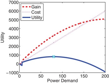
Fig. 3. The gain, cost, and intermediate utility versus the power demand with the optimal demand
![]() $d_{i}^{\star}=80$
when the reference price p
r
= 30.
$d_{i}^{\star}=80$
when the reference price p
r
= 30.
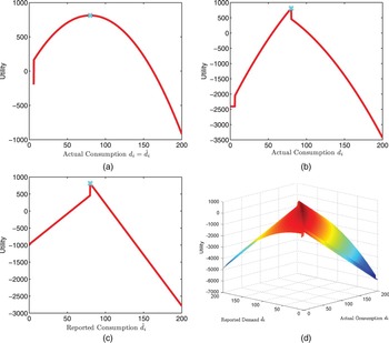
Fig. 4. The incentive compatible performance of the proposed scheme when the optimal demand
![]() $d_{i}^{\star} = 80$
and the reference price p
r
= 30: (a) the utility versus the real-power consumption d
i
when the reported demand
$d_{i}^{\star} = 80$
and the reference price p
r
= 30: (a) the utility versus the real-power consumption d
i
when the reported demand
![]() $\hat{d}_{i} = d_{i}$
; (b) the utility versus the real-power consumption d
i
when the reported demand
$\hat{d}_{i} = d_{i}$
; (b) the utility versus the real-power consumption d
i
when the reported demand
![]() $\hat{d}_{i} = d_{i}^{\star} = 80$
; (c) the utility versus the reported demand
$\hat{d}_{i} = d_{i}^{\star} = 80$
; (c) the utility versus the reported demand
![]() $\hat{d}_{i}$
when the real-power consumption
$\hat{d}_{i}$
when the real-power consumption
![]() $\hat{d}_{i} = d_{i}^{\star} = 80$
; (d) the utility versus the reported demand
$\hat{d}_{i} = d_{i}^{\star} = 80$
; (d) the utility versus the reported demand
![]() $\hat{d}_{i}$
and real-power consumption d
i
.
$\hat{d}_{i}$
and real-power consumption d
i
.
From the above discussions, we can see that, with the proposed incentive compatible scheme, customers are motivated to report and consume the optimal demand to achieve the maximal utility. Such an incentive compatible property is mainly because of the use of the punishment term in (4). Without the punishment, customers may not report and consume the optimal demand. In Fig. 5, we show the customer's utility versus the reported demand and real-power consumption
![]() $\lpar \hat{d_{i}}\comma \; d_{i}\rpar $
by assuming that there is no punishment term in the utility function, i.e., the cost function is defined as p
r
d
i
. As shown in Fig. 5, we can see that for any given
$\lpar \hat{d_{i}}\comma \; d_{i}\rpar $
by assuming that there is no punishment term in the utility function, i.e., the cost function is defined as p
r
d
i
. As shown in Fig. 5, we can see that for any given
![]() $\hat{d}_{i}$
, the utility is maximized when
$\hat{d}_{i}$
, the utility is maximized when
![]() $d_{i}=d_{i}^{\star}$
. However, the utility function is independent from
$d_{i}=d_{i}^{\star}$
. However, the utility function is independent from
![]() $\hat{d}_{i}$
, i.e., the utility function is constant in terms of
$\hat{d}_{i}$
, i.e., the utility function is constant in terms of
![]() $\hat{d}_{i}$
. In such a case, customers have no incentive to report true optimal demand since their utility functions will not be affected no matter what demand they report to the power substation. Therefore, it is very important for us to involve the punishment term in the cost function as in (4).
$\hat{d}_{i}$
. In such a case, customers have no incentive to report true optimal demand since their utility functions will not be affected no matter what demand they report to the power substation. Therefore, it is very important for us to involve the punishment term in the cost function as in (4).
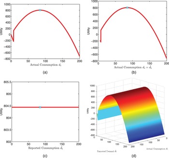
Fig. 5. The non-incentive-compatible performance of the scheme without punishment in the utility function: (a) the utility versus the real-power consumption d
i
when the reported demand
![]() $\hat{d}_{i} = d_{i}$
; (b) the utility versus the real-power consumption d
i
when the reported demand
$\hat{d}_{i} = d_{i}$
; (b) the utility versus the real-power consumption d
i
when the reported demand
![]() $\hat{d}_{i} = d_{i}^{\star} = 85$
; (c) the utility versus the reported demand
$\hat{d}_{i} = d_{i}^{\star} = 85$
; (c) the utility versus the reported demand
![]() $\hat{d}_{i}$
when the real-power consumption
$\hat{d}_{i}$
when the real-power consumption
![]() $\hat{d}_{i} = d_{i}^{\star} = 85$
; (d) the utility versus the reported demand
$\hat{d}_{i} = d_{i}^{\star} = 85$
; (d) the utility versus the reported demand
![]() $\hat{d}_{i}$
and real-power consumption d
i
.
$\hat{d}_{i}$
and real-power consumption d
i
.
We then evaluate the performance of the proposed dynamic pricing algorithm in Fig. 6. Fig. 6(a) shows the total demand from customers versus time when the target total demand remains constant over time. We can see that with the proposed dynamic pricing algorithm, the total demand from customers quickly converges to the target total demand with the difference between the total demand and the target demand <1% of the target demand. Fig. 6(b) illustrates the response time of the dynamic pricing subject to sudden change of target demand. We can see from Fig. 6(b) that the proposed algorithm can quickly respond to the change of target demand through adjusting the price accordingly, which fully demonstrate the efficiency and effectiveness of the proposed dynamic pricing algorithm.
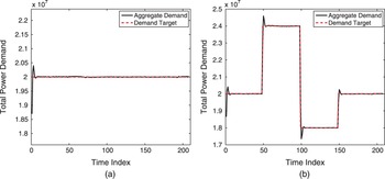
Fig. 6. The demand controlling performance of the proposed scheme: (a) constant target demand; (b) time-varying target demand.
Since the proposed game-theoretic scheme is incentive compatible, customers are motivated to report and consume their optimal demands to achieve best utilities. In such a case, the real consumption of the customer should be the same as the reported demand. Nevertheless, in some scenarios, customers' consumptions may be different from the reported demands. In Fig. 7, we evaluate the effect of customers' deviation on the total demand. We assume that there is a portion of customers deviating from their reported demands. The customer who deviates will consume (1 + ε) times of the reported demand, i.e.,
![]() $d_{i}=\lpar 1+\epsilon\rpar \hat{d}_{i}$
, where ε satisfies Gaussian distribution with zero mean and 0.2 variance. From Fig. 7, we can see that even with 25% of customers deviating from the reported demands, the actual total consumption is still close to the aggregate reported demand. Therefore, the proposed scheme is very robust to the customers' deviation.
$d_{i}=\lpar 1+\epsilon\rpar \hat{d}_{i}$
, where ε satisfies Gaussian distribution with zero mean and 0.2 variance. From Fig. 7, we can see that even with 25% of customers deviating from the reported demands, the actual total consumption is still close to the aggregate reported demand. Therefore, the proposed scheme is very robust to the customers' deviation.
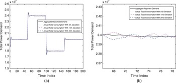
Fig. 7. (a) The robustness performance against real consumption deviation; (b) zoom-in figure of (a).
In the last simulation, we compare our dynamic pricing algorithm with the constant pricing algorithm. We obtain the hourly total consumption of CAISO on October 31, 2011 from [31] and generate the 5-min-based total consumption by interpolating the hourly data. Since the day-ahead price of CAISO on October 31, 2011 is around $ 30, we assume that the real total consumption is the outcome of the constant pricing scheme and use the interpolated data to train the parameters W and Q in (16) and the AR coefficient in (18). As shown in Fig. 8, the total demand using constant pricing scheme (blue dot curve) matches well with the real total consumption of CAISO (pink dash-dot curve), which in some senses validates the utility function and the AR modeling. Nevertheless, the constant pricing algorithm cannot adapt well to the change of the target demand (red dash curve), which may lead to power outage or power inefficiency. On the other hand, with our proposed algorithm, the aggregate demand closely follows the target demand. Moreover, since the aggregate reported demand is an accurate estimate of the real consumption and is known ahead of time, the power substation can generate the corresponding amount of power and thus greatly improve the system efficiency and reduce the risk of outage.
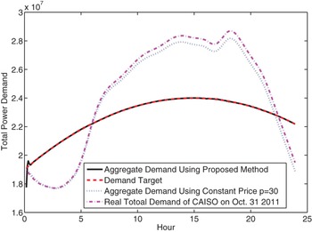
Fig. 8. The performance comparison with constant pricing algorithm.
V. CONCLUSIONS
In this paper, we have proposed a game-theoretic demand response scheme that can transform the difficult and complex centralized demand forecasting problem into an easy demand reporting mechanism. Such a game-theoretic scheme is shown to be incentive compatible which can enforce the selfish customers to report and consume their true optimal demands. Moreover, the proposed scheme leads to the desired solution from both system designer's and customers' perspective since the solution is not only social welfare maximizing but also proportionally fair in terms of utility function. Furthermore, we have proposed a simple dynamic pricing algorithm for the power substation to effectively control the total demand from customers to meet a target demand curve. With the proposed algorithm, the power substation can obtain an accurate estimate of the real consumption ahead of time and generate the corresponding amount of power, and thus greatly improve the system efficiency and reduce the risk of outage.
Yan Chen received the Bachelor's degree from the University of Science and Technology of China in 2004, the M. Phil. degree from Hong Kong University of Science and Technology (HKUST) in 2007, and the Ph.D. degree from the University of Maryland College Park in 2011. His current research interests are in data science, network science, game theory, social learning, and networking, as well as signal processing and wireless communications. He is the recipient of multiple honors and awards including best paper award from IEEE GLOBECOM in 2013, Future Faculty Fellowship, and Distinguished Dissertation Fellowship Honorable Mention from the Department of Electrical and Computer Engineering in 2010 and 2011, respectively, Finalist of Dean's Doctoral Research Award from A. James Clark School of Engineering at the University of Maryland in 2011, and Chinese Government Award for outstanding students abroad in 2011.
W. Sabrina Lin received the Ph.D. degree from the Electrical and Computer Engineering Department, the University of Maryland, College Park in 2009. She received the B.S. and M.S. degrees in Electrical Engineering from National Taiwan University in 2002 and 2004, respectively. Currently, she is with IBM Research Division, Yorktown Heights, NY. Her research interests are in the area of information security and forensics, multimedia signal processing and multimedia social network analysis. She received the University of Maryland Innovation Award in 2011 and has co-authored the book Behavior Dynamics in Media-Sharing Social Networks (Cambridge University Press, 2011).
Feng Han received the B.S. and M.S. degrees from Tsinghua University, Beijing, China, in 2007 and 2009, respectively; and the Ph.D. degree from the University of Maryland, College Park, MD, USA, in 2013, all in Electrical Engineering. Currently, he is a senior engineer with Corporate Research and Development, Qualcomm Inc., San Diego, CA. His research interests include wireless communications and networking, game theory, signal processing, and communication theory. He is a recipient of the first prize in the 19th Chinese Mathematical Olympiad, the Best Thesis Award of Tsinghua University, the honor of Excellent Graduate of Tsinghua University, the A. James Clark School of Engineering Distinguished Graduate Fellowship in 2009 and the Future Faculty Fellowship in 2012, both from the University of Maryland, College Park. His work on time reversal technique was recognized by the university-level Invention of the Year Award and The Jimmy H. C. Lin Invention Award, both at the University of Maryland in 2013, and his work on the MIMO system received a Best Paper Award for at IEEE WCNC’08.
Yu-Han Yang received his B.S. degree in Electrical Engineering in 2004, M.S. degree in Computer Science and Communication Engineering in 2007, from National Taiwan University, Taipei, Taiwan, and Ph.D. degree in Electrical and Computer Engineering in 2013 from the University of Maryland, College Park, USA. He is currently a Senior Engineer in modem systems with Qualcomm Incorporated, San Diego, CA. His research interests are in the area of wireless communications and signal processing, including MIMO beamforming, multi-user detection, and power control. He is a recipient of Study Abroad Scholarship from Taiwan (R.O.C.) Government in 2009–2010. He received the University of Maryland Innovation Award in 2013.
Zoltan Safar received the University Diploma in Electrical Engineering from the Technical University of Budapest, Budapest, Hungary, in 1996, and the M.S. and Ph.D. degrees in Electrical and Computer Engineering from the University of Maryland, College Park, MD, USA, in 2001 and 2003, respectively. After graduation, he was an Assistant Professor with the Department of Innovation, IT University of Copenhagen, Copenhagen, Denmark, until March 2005. Then, he joined Nokia, Copenhagen, Denmark, where he worked as a Senior Engineer on 3GPP Long Term Evolution (LTE) receiver algorithmdesign. From September 2007, he was a Senior Engineer with Samsung Electro-Mechanics, Atlanta, GA, USA, developing physical-layer signal processing algorithms for next-generation wireless communication systems. In February 2010, he became a Senior Software Engineer with Bloomberg L.P., NY, USA, and he designed and implemented software systems for monitoring, configuration and maintenance of the company's private communication network. Since October 2010, he has been with the Department of Electrical and Computer Engineering, University of Maryland, where he is the Director of the MS in Telecommunications program. His research interests include wireless communications and statistical signal processing, with particular focus on multi-antenna wireless communication systems, OFDM, and receiver algorithm design. Dr. Safar received the Outstanding Systems Engineering Graduate Student Award from the Institute for Systems Research, the University of Maryland, in 2003, and the Invention of the Year Award (together with W. Su and K. J. R. Liu) from the University of Maryland, in 2004.
K. J. Ray Liu was named a Distinguished Scholar-Teacher of University of Maryland, College Park, in 2007, where he is Christine Kim Eminent Professor of Information Technology. He leads the Maryland Signals and Information Group conducting research encompassing broad areas of signal processing and communications with recent focus on cooperative and cognitive communications, social learning and network science, information forensics and security, and green information and communications technology. Dr. Liu was a Distinguished Lecturer, recipient of IEEE Signal Processing Society 2009 Technical Achievement Award and various best paper awards. He also received various teaching and research recognitions from the University of Maryland including university-level Invention of the Year Award; and Poole and Kent Senior Faculty Teaching Award, Outstanding Faculty Research Award, and Outstanding Faculty Service Award, all from A. James Clark School of Engineering. An ISI Highly Cited Author, Dr. Liu is a Fellow of IEEE and AAAS. Dr. Liu is Past President of IEEE Signal Processing Society where he has served as the President, Vice President — Publications and Board of Governor. He was the Editor-in-Chief of IEEE Signal Processing Magazine and the founding Editor-in-Chief of EURASIP Journal on Advances in Signal Processing.


