


1. Introduction
Soft deformable objects – e.g. cells and capsules – are ubiquitous in biology and biotechnology, serving as building blocks of complex interacting systems typically driven by external flows (Lac, Morel & Barthès-Biesel Reference Lac, Morel and Barthès-Biesel2007; Barthes-Biesel Reference Barthes-Biesel2016; Bah, Bilal & Wang Reference Bah, Bilal and Wang2020; Owen et al. Reference Owen2023). In computational studies, they serve as simplified analogues for more intricate biological cells – such as red blood cells and circulating tumour cells – helping researchers examine cellular behaviour and mechanics (Krüger Reference Krüger2012; Gekle Reference Gekle2016; Balogh et al. Reference Balogh, Gounley, Roychowdhury and Randles2021; Huet & Wachs Reference Huet and Wachs2023). Their widespread applications demand a comprehensive understanding of capsule properties, achieved through the combined strengths of theoretical, experimental and computational approaches (Shen et al. Reference Shen, Fischer, Farutin, Vlahovska, Harting and Misbah2018; Chen et al. Reference Chen, Singh, Schirrmann, Zhou, Chernyavsky and Juel2023). Recent advances highlight the efficacy of microfluidic systems in separating cells by size and deformability, enabling the enrichment of specific cell types and facilitating detailed characterisation (Zhu et al. Reference Zhu, Rorai, Mitra and Brandt2014; Häner et al. Reference Häner, Vesperini, Salsac, Le Goff and Juel2021; Lu et al. Reference Lu, Wang, Salsac, Barthès-Biesel, Wang and Sui2021; Waters Reference Waters2024).
Substantial research on capsule deformation and dynamics in non-inertial flows has arisen from their significance in microcirculation (e.g. capillary blood flow) and microfluidic applications. Early work by Barthès-Biesel and Rallison employed thin-shell theory to model elastic capsules in slow shear flows, assuming small deformations (Barthes-Biesel & Rallison Reference Barthes-Biesel and Rallison1981). Pozrikidis extended this approach using the boundary integral method to incorporate finite deformations, fluid viscosity variations and bending stresses (Pozrikidis Reference Pozrikidis1995, Reference Pozrikidis2001). More recently, Balogh and Bagchi used the front-tracking method to investigate red blood cell behaviour in complex networks resembling human microcirculation (Balogh & Bagchi Reference Balogh and Bagchi2017, Reference Balogh and Bagchi2018, Reference Balogh and Bagchi2019). Research has also addressed the mechanical and rheological properties of elastic capsule suspensions – through analytical, experimental and numerical methods – building on Batchelor’s foundational work on particle stress tensors (Batchelor Reference Batchelor1970; Barthes-Biesel & Rallison Reference Barthes-Biesel and Rallison1981; Ramanujan & Pozrikidis Reference Ramanujan and Pozrikidis1998; Walter, Rehage & Leonhard Reference Walter, Rehage and Leonhard2001). Subsequent studies explored rheological characteristics of elastic capsule suspensions in non-inertial regimes, elucidating the influence of the particle dynamics (Takeishi et al. Reference Takeishi, Rosti, Imai, Wada and Brandt2019), as well as the roles of strainhardening and membrane viscosity in the suspension rheology (Aouane, Scagliarini & Harting Reference Aouane, Scagliarini and Harting2021; Guglietta et al. Reference Guglietta, Pelusi, Sega, Aouane and Harting2023).
Deformable capsules exhibit nonlinear elastic behaviour, which gives rise to complex hydrodynamic interactions when they come into close proximity (Barthès-Biesel Reference Barthès-Biesel2009). When capsules come near each other, a thin liquid film may form between their membranes, which, under high shear forces, can result in membrane deformation or even damage (El Mertahi et al. Reference El Mertahi, Grandmaison, Dupont, Jellali, Brancherie and Salsac2024). The hydrodynamic interaction among these flowing objects can give rise to emergent non-equilibrium structures (Lushi, Wioland & Goldstein Reference Lushi, Wioland and Goldstein2014; Goto & Tanaka Reference Goto and Tanaka2015; Yeo, Lushi & Vlahovska Reference Yeo, Lushi and Vlahovska2015) such as log-rolling chains of rigid spheres aligned along the vorticity direction in shear flows (Cheng et al. Reference Cheng, Xu, Rice, Dinner and Cohen2012), spontaneous alignment in attractive emulsions and colloidal suspensions (Migler Reference Migler2001; Montesi, Peña & Pasquali Reference Montesi, Peña and Pasquali2004; Varga et al. Reference Varga, Grenard, Pecorario, Taberlet, Dolique, Manneville, Divoux, McKinley and Swan2019; Millett Reference Millett2024) and crystal-like arrangements in red blood cell suspensions (Shen et al. Reference Shen, Fischer, Farutin, Vlahovska, Harting and Misbah2018). Such emergent structures not only affect the short-range dynamics but also govern large-scale suspension behaviour, including aggregation, diffusion and rheology (Morris & Brady Reference Morris and Brady1996; Griffiths & Stone Reference Griffiths and Stone2012; Matsunaga et al. Reference Matsunaga, Imai, Yamaguchi and Ishikawa2016; Gai et al. Reference Gai, Huet, Gong and Wachs2025). Conversely, transition from deterministic to random behaviour when varying object deformability has already been reported in a few previous contexts such as red blood cell distributions within networks (Shen et al. Reference Shen, Plouraboué, Lintuvuori, Zhang, Abbasi and Misbah2023), or transition from a leapfrog motion (Lac & Barthès-Biesel Reference Lac and Barthès-Biesel2008) to the minuet dynamics (Hu et al. Reference Hu, Lei, Salsac and Barthès-Biesel2020) of binary capsule interactions.
Understanding binary hydrodynamic interactions is essential for studying capsule suspensions, due to their significant influence on capsule collective migration and rheological behaviours (Krüger Reference Krüger2012; Abbasi et al. Reference Abbasi, Farutin, Ez-Zahraouy, Benyoussef and Misbah2021). Lac et al. (Reference Lac, Morel and Barthès-Biesel2007) conducted the pioneering three-dimensional simulations of the binary interaction between a pair of spherical capsules in a shear flow, with their centres initially positioned on the same shear plane. It was shown that one capsule overpassed the other and shifted back to the flow axis as it moved away, which is referred to as leapfrog motion. The crossing results in an irreversible shift in the capsule trajectory along the shear gradient, which is believed to contribute to self-diffusion. The same configuration was revisited with two red blood cells (Omori et al. Reference Omori, Ishikawa, Imai and Yamaguchi2013) and vesicles (Gires et al. Reference Gires, Srivastav, Misbah, Podgorski and Coupier2014), where the leapfrog motion was also observed. Doddi & Bagchi used the front-tracking method to investigate the binary interaction of capsules in an inertial shear flow and found that, instead of crossing as in the zero Reynolds number case, inertia induces a reversed motion of capsules (Doddi & Bagchi Reference Doddi and Bagchi2008a ,Reference Doddi and Bagchi b ). This spiralling motion was attributed to the limited size of the computational domain. Pranay et al. (Reference Pranay, Anekal, Hernandez-Ortiz and Graham2010) considered the binary interaction of capsules in a polymeric fluid, showing that the trajectory shift can be decreased when the capsule deformability is low. Singh & Sarkar (Reference Singh and Sarkar2015) further elucidated that the stiffness ratio of the two capsules can affect the trajectory shift. Pair formation has been reported in inertial migration of both rigid and deformable particles in pipe flows, accompanied by a characteristic damped oscillatory dynamics during the pairing process which was attributed to inertial effects (Schaaf, Rühle & Stark Reference Schaaf, Rühle and Stark2019; Patel & Stark Reference Patel and Stark2021). Regarding capsule pair interactions, the pair stability has been shown to depend strongly on capsule softness, size, heterogeneity and initial relative position (Owen & Krüger Reference Owen and Krüger2022; Thota, Owen & Krüger Reference Thota, Owen and Krüger2023; Owen, Thota & Krüger Reference Owen, Thota and Krüger2024).
From another point of view, the binary interaction of capsules in different shear planes has been simulated and discussed by Lac & Barthès-Biesel (Reference Lac and Barthès-Biesel2008). In this case, a sideways leapfrog motion was noticed and then later confirmed for vesicles by Gires et al. (Reference Gires, Srivastav, Misbah, Podgorski and Coupier2014). Hu et al. (Reference Hu, Lei, Salsac and Barthès-Biesel2020) found a new interaction motion, the minuet motion, for the capsule pair initially closely positioned at two different shear planes. Within this interaction mode, the capsule pair can remain stable for a long time while dancing a minuet, especially for less deformable capsules. The minuet motion leads capsules to closely interact and deform significantly. When they separate, the two capsules can reverse direction. The reason for this minuet motion was attributed to the pressure evolution in the lubrication layer during the crossing and separating process.
Despite the insights gained, significant gaps persist in our understanding of the interaction mechanisms of a pair of capsules in different shear planes. In this study, we investigate the soft hydrodynamic interactions of spherical capsules and report a previously unrecognised capturing regime in the capsule dynamics. Unlike the leapfrog and minuet motions, this novel regime features the formation of a stable doublet, where the satellite capsule remains aligned with a reference capsule along the vorticity direction. Using high-fidelity, particle-resolved numerical simulations, we address the following key questions: $(i)$
Does a stable binary doublet exist, and what is the mechanism behind its formation?
$(i)$
Does a stable binary doublet exist, and what is the mechanism behind its formation? $(\textit{ii})$
How are the leapfrog, minuet and capturing regimes connected?
$(\textit{ii})$
How are the leapfrog, minuet and capturing regimes connected? $(\textit{iii})$
What insights can binary interactions provide for our understanding of the multi-body dynamics?
$(\textit{iii})$
What insights can binary interactions provide for our understanding of the multi-body dynamics?
This manuscript is organised as follows. Section 2 introduces the governing equations and the membrane model for deformable capsules. In § 3, we define the key physical quantities and the relevant dimensionless parameters. Section 4 describes the numerical set-up used for simulating binary capsule interactions. In § 5, we present the physical validation of the numerical solver. Section 6 analyses the binary interaction of deformable capsules in shear flow, focusing on interaction regimes, trajectories and deformations. We analyse the capturing regime through kinematic signatures and parametric sensitivity, and elucidate its gentle, stable nature. The mechanisms driving satellite capture and the resulting nonlinear hydrodynamic ordering and flow perturbations are discussed. Section 7 extends the discussion to ternary interactions of elastic capsules. Finally, § 8 summarises the main findings and outlines perspectives for future work.
2. Governing equations and membrane model
The capsule membrane $\varGamma$
is modelled as an infinitely thin interface, enclosing a region filled with an incompressible Newtonian fluid of constant viscosity and density. The motion of the fluid is governed by mass and momentum conservation
$\varGamma$
is modelled as an infinitely thin interface, enclosing a region filled with an incompressible Newtonian fluid of constant viscosity and density. The motion of the fluid is governed by mass and momentum conservation
 \begin{align} \tilde {\boldsymbol{\nabla }} \boldsymbol{\cdot }\boldsymbol{\tilde {u}} = 0, \\[-28pt] \nonumber \end{align}
 \begin{align} \frac {\partial \boldsymbol{\tilde {u}}}{\partial \tilde {t}} = -\frac {1}{\tilde {\rho }} \tilde {\boldsymbol{\nabla }} \tilde {p} + \tilde {\nu } \tilde {{\nabla} }^2 \boldsymbol{\tilde {u}} + \frac {1}{\tilde {\rho }} \boldsymbol{\tilde {f}_b}. \\[2pt] \nonumber \end{align}
Here, $\boldsymbol{\tilde {u}}$
and
$\boldsymbol{\tilde {u}}$
and $\tilde {p}$
denote the flow velocity and pressure, respectively, and
$\tilde {p}$
denote the flow velocity and pressure, respectively, and $\tilde {\rho }$
is the fluid density. The kinematic viscosity is defined as
$\tilde {\rho }$
is the fluid density. The kinematic viscosity is defined as $\tilde {\nu } = \tilde {\mu }/\tilde {\rho }$
, with
$\tilde {\nu } = \tilde {\mu }/\tilde {\rho }$
, with $\tilde {\mu }$
being the dynamic viscosity. Dimensional quantities are denoted by a tilde (
$\tilde {\mu }$
being the dynamic viscosity. Dimensional quantities are denoted by a tilde ( $\sim$
). We consider the Stokes regime and explicitly account for the elastic force acting on the membrane. The elastic force generates a localised stress into the fluid as a body force
$\sim$
). We consider the Stokes regime and explicitly account for the elastic force acting on the membrane. The elastic force generates a localised stress into the fluid as a body force $\boldsymbol{\tilde {f}_b}$
that reads
$\boldsymbol{\tilde {f}_b}$
that reads
 \begin{align} \boldsymbol{\tilde {f}_b} = \boldsymbol{\tilde {F}_{\textit{elastic}}} \tilde {\delta }(\boldsymbol{\tilde {x}} - \boldsymbol{\tilde {x}_{0}}), \end{align}
where $\tilde {\boldsymbol{x}} = (\tilde {x}, \tilde {y}, \tilde {z})$
is the spatial coordinate, and
$\tilde {\boldsymbol{x}} = (\tilde {x}, \tilde {y}, \tilde {z})$
is the spatial coordinate, and $\tilde {\delta }(\boldsymbol{\tilde {x}} - \boldsymbol{\tilde {x}_{0}})$
the Dirac distribution centred at position
$\tilde {\delta }(\boldsymbol{\tilde {x}} - \boldsymbol{\tilde {x}_{0}})$
the Dirac distribution centred at position $\boldsymbol{\tilde {x}_{0}}$
on the membrane surface, i.e.
$\boldsymbol{\tilde {x}_{0}}$
on the membrane surface, i.e. $\boldsymbol{\tilde {x}_{0}} \in \varGamma$
.
$\boldsymbol{\tilde {x}_{0}} \in \varGamma$
.
The shear and area-dilatation stresses in the membrane are modelled using thin-shell theory, which is briefly outlined here (for a comprehensive derivation, the reader is referred to Barthes-Biesel & Rallison Reference Barthes-Biesel and Rallison1981). In this study, the elastic behaviour of the membrane is described using the Skalak constitutive law for which the associated surface strain energy $\tilde {W_s}$
is given by
$\tilde {W_s}$
is given by
 \begin{align} \tilde {W_s} = \frac {\tilde {E_s}}{4} \big ( I_1^2 + 2I_1 - 2I_2 + CI_2^2 \big ), \end{align}
where $\tilde {E_s}$
is the membrane shear modulus and the two invariants
$\tilde {E_s}$
is the membrane shear modulus and the two invariants $I_{1,2}$
 \begin{align} I_1 = \lambda _1^2 + \lambda _2^2 - 2, \,\,\, \,\,\, \,\,\, I_2 = \lambda _1^2 \lambda _2^2 - 1, \end{align}
are related to $\lambda _{1,2}$
, the principal stretches along the two tangential directions. The area-dilatation modulus is set to
$\lambda _{1,2}$
, the principal stretches along the two tangential directions. The area-dilatation modulus is set to $C = 1$
, which penalises large changes in surface area (Pozrikidis Reference Pozrikidis1995). The membrane elastic stresses
$C = 1$
, which penalises large changes in surface area (Pozrikidis Reference Pozrikidis1995). The membrane elastic stresses $\tilde {\sigma }_{i,j}$
are then derived from the strain energy function
$\tilde {\sigma }_{i,j}$
are then derived from the strain energy function $\tilde {W_s}$
as
$\tilde {W_s}$
as
 \begin{align} \tilde {\sigma }_{i,j} = \frac {1}{\lambda _j} \frac {\partial \tilde {W_s}}{\partial \lambda _i}, \qquad i, j \in \{1,2\}, \quad i \neq j. \end{align}
Once the membrane elastic stress tensor is obtained, the resulting elastic force exerted by the membrane on the surrounding fluid is computed as
 \begin{align} \boldsymbol{\tilde {F}_{\textit{elastic}}} = \tilde {\boldsymbol{\nabla }} \boldsymbol{\cdot }\boldsymbol{\tilde {\sigma }}. \end{align}
3. Physical quantities and dimensionless numbers
In this study, we consider a pair of elastic capsules suspended in a Stokes flow subjected to simple shear. The capillary number is defined as $ {\mathcal{C}a} = \tilde {\mu } \tilde {\dot {\gamma }} \tilde {r}_0/\tilde {E_s}$
, where
$ {\mathcal{C}a} = \tilde {\mu } \tilde {\dot {\gamma }} \tilde {r}_0/\tilde {E_s}$
, where $\tilde {\mu }$
is the dynamic viscosity,
$\tilde {\mu }$
is the dynamic viscosity, $\tilde {\dot {\gamma }}$
is the shear rate,
$\tilde {\dot {\gamma }}$
is the shear rate, $\tilde {r}_0$
is the characteristic length scale (radius of the initial spherical capsule) and
$\tilde {r}_0$
is the characteristic length scale (radius of the initial spherical capsule) and $\tilde {E_s}$
is the elastic modulus of the capsule membrane. In a simple shear flow, the dimensional shear rate is defined as
$\tilde {E_s}$
is the elastic modulus of the capsule membrane. In a simple shear flow, the dimensional shear rate is defined as $\tilde {\dot {\gamma }} = \tilde {U}_0/\tilde {L}$
, where
$\tilde {\dot {\gamma }} = \tilde {U}_0/\tilde {L}$
, where $\tilde {U}_0$
is the imposed velocity difference between the two moving solid boundaries and
$\tilde {U}_0$
is the imposed velocity difference between the two moving solid boundaries and $\tilde {L}$
is the normal distance between the two moving solid boundaries, here, the side length of the cubic computational domain. The Reynolds number
$\tilde {L}$
is the normal distance between the two moving solid boundaries, here, the side length of the cubic computational domain. The Reynolds number ${\textit{Re}} = \tilde {\rho } \tilde {\dot {\gamma }} \tilde {r}_0^2/\tilde {\mu }$
is set to
${\textit{Re}} = \tilde {\rho } \tilde {\dot {\gamma }} \tilde {r}_0^2/\tilde {\mu }$
is set to $0.1$
. Inertia is neglected by omitting the convective term in the Navier–Stokes equations, as appropriate for Stokes flow. We analyse several physical quantities that characterise the binary interaction of capsules. These include capsule trajectory, velocity, acceleration, interaction frequency, deformation parameter (
$0.1$
. Inertia is neglected by omitting the convective term in the Navier–Stokes equations, as appropriate for Stokes flow. We analyse several physical quantities that characterise the binary interaction of capsules. These include capsule trajectory, velocity, acceleration, interaction frequency, deformation parameter ( $D$
) and particle-induced stress (
$D$
) and particle-induced stress ( $\varSigma ^p$
), among others. Below, we briefly describe the methods used to compute and non-dimensionalise these quantities.
$\varSigma ^p$
), among others. Below, we briefly describe the methods used to compute and non-dimensionalise these quantities.
The trajectory, velocity, acceleration and frequency are non-dimensionalised using the characteristic length scale $\tilde {r}_0$
, characteristic velocity scale
$\tilde {r}_0$
, characteristic velocity scale $\tilde {\dot {\gamma }}\tilde {r}_0$
and characteristic time scale
$\tilde {\dot {\gamma }}\tilde {r}_0$
and characteristic time scale $1/\tilde {\dot {\gamma }}$
. Capsule deformation is quantified using its moment of inertia tensor. Specifically, we consider an equivalent ellipsoid that shares the same inertia tensor,
$1/\tilde {\dot {\gamma }}$
. Capsule deformation is quantified using its moment of inertia tensor. Specifically, we consider an equivalent ellipsoid that shares the same inertia tensor, $\tilde {\mathcal{I}}$
, as the capsule. With the three eigenvalues (
$\tilde {\mathcal{I}}$
, as the capsule. With the three eigenvalues ( $\tilde {\zeta }_1 \lt \tilde {\zeta }_2 \lt \tilde {\zeta }_3$
) of
$\tilde {\zeta }_1 \lt \tilde {\zeta }_2 \lt \tilde {\zeta }_3$
) of $\tilde {\mathcal{I}}$
, we can compute the semi-axis lengths:
$\tilde {\mathcal{I}}$
, we can compute the semi-axis lengths: $\tilde {r}_1, \tilde {r}_2$
and
$\tilde {r}_1, \tilde {r}_2$
and $\tilde {r}_3$
(Ramanujan & Pozrikidis Reference Ramanujan and Pozrikidis1998; Guglietta et al. Reference Guglietta, Pelusi, Sega, Aouane and Harting2023). Here,
$\tilde {r}_3$
(Ramanujan & Pozrikidis Reference Ramanujan and Pozrikidis1998; Guglietta et al. Reference Guglietta, Pelusi, Sega, Aouane and Harting2023). Here, $\tilde {r}_1$
and
$\tilde {r}_1$
and $\tilde {r}_3$
are the longest and shortest semi-axis lengths in the shear plane (
$\tilde {r}_3$
are the longest and shortest semi-axis lengths in the shear plane ( $x$
–
$x$
– $y$
plane), and
$y$
plane), and $\tilde {r}_2$
denotes the radius along the vorticity direction, along the axis normal to the shear plane (i.e.
$\tilde {r}_2$
denotes the radius along the vorticity direction, along the axis normal to the shear plane (i.e. $z$
-axis in our convention choice). The Taylor deformation factor is then defined as
$z$
-axis in our convention choice). The Taylor deformation factor is then defined as
 \begin{align} D = \frac {\tilde {r}_1-\tilde {r}_3}{\tilde {r}_1+\tilde {r}_3}. \end{align}
The bulk excess stress of the capsule, $\varSigma ^p$
, is calculated following Batchelor’s formulation for Stokes flow (Batchelor Reference Batchelor1970). The particle stress tensor
$\varSigma ^p$
, is calculated following Batchelor’s formulation for Stokes flow (Batchelor Reference Batchelor1970). The particle stress tensor $\varSigma ^p$
, which accounts for capsule–capsule interactions, is computed using the Lagrangian nodal forces acting on the capsule surface, as described by Krüger (Reference Krüger2012) and Gross, Krüger & Varnik (Reference Gross, Krüger and Varnik2014)
$\varSigma ^p$
, which accounts for capsule–capsule interactions, is computed using the Lagrangian nodal forces acting on the capsule surface, as described by Krüger (Reference Krüger2012) and Gross, Krüger & Varnik (Reference Gross, Krüger and Varnik2014)
 \begin{align} \tilde {\varSigma }_{\alpha \beta }^p = -\frac {1}{\tilde {V}} \sum _{i = 1}^{N}\sum _{j}^{N_{\textit{ele}}}\frac {1}{2} \big(\tilde {F}_\alpha ^{i,j}\tilde {r}_\beta ^{i,j} + \tilde {F}_\beta ^{i,j}\tilde {r}_\alpha ^{i,j} \big), \end{align}
where $\alpha$
and
$\alpha$
and $\beta$
denote Cartesian directions (
$\beta$
denote Cartesian directions ( $x$
,
$x$
, $y$
or
$y$
or $z$
),
$z$
), $N$
is the number of capsules within the control volume
$N$
is the number of capsules within the control volume $\tilde {V}$
and
$\tilde {V}$
and $N_{\textit{ele}}$
is the number of triangular elements on each capsule surface. Here,
$N_{\textit{ele}}$
is the number of triangular elements on each capsule surface. Here, $\tilde {F}^{i,j}$
corresponds to the Lagrangian force acting on the node located at position vector
$\tilde {F}^{i,j}$
corresponds to the Lagrangian force acting on the node located at position vector $\tilde {\boldsymbol{r}}^{i,j}$
. Specifically, the dimensionless particle shear stress, as well as the first and second normal stress differences, are defined as follows:
$\tilde {\boldsymbol{r}}^{i,j}$
. Specifically, the dimensionless particle shear stress, as well as the first and second normal stress differences, are defined as follows:
 \begin{align} \varSigma _{\textit{xy}}^{p} = \frac {\tilde {\varSigma }_{\textit{xy}}^p}{\tilde {\mu } \tilde {\dot {\gamma }} \phi _t}, \quad N_1 = \frac {\tilde {\varSigma }_{\textit{xx}}^p - \tilde {\varSigma }_{\textit{yy}}^p}{\tilde {\mu } \tilde {\dot {\gamma }} \phi _t}, \quad N_2 = \frac {\tilde {\varSigma }_{\textit{yy}}^p - \tilde {\varSigma }_{zz}^p}{\tilde {\mu } \tilde {\dot {\gamma }} \phi _t}, \end{align}
where $\phi _t$
denotes the total volume fraction of the capsules.
$\phi _t$
denotes the total volume fraction of the capsules.
4. Numerical method and set-up
The numerical set-up for the binary capsule interaction is depicted in figure 1. A simple shear flow is imposed along the $x$
-axis, characterised by a constant shear rate
$x$
-axis, characterised by a constant shear rate $\tilde {\dot {\gamma }} = \tilde {U}_0/\tilde {L} =1\, \textrm{s}^{-1}$
. The simulation is conducted within a cubic domain
$\tilde {\dot {\gamma }} = \tilde {U}_0/\tilde {L} =1\, \textrm{s}^{-1}$
. The simulation is conducted within a cubic domain $\mathcal{D}$
of edge length
$\mathcal{D}$
of edge length $\tilde {L} = 77\tilde {r}_0$
, where
$\tilde {L} = 77\tilde {r}_0$
, where $\tilde {r}_0$
is the radius of the reference (i.e. largest) capsule. The domain boundaries are aligned with the coordinate axes: left/right (
$\tilde {r}_0$
is the radius of the reference (i.e. largest) capsule. The domain boundaries are aligned with the coordinate axes: left/right ( $x$
), top/bottom (
$x$
), top/bottom ( $y$
) and front/back (
$y$
) and front/back ( $z$
). Dirichlet conditions are imposed on the top and bottom boundaries to enforce a linear shear profile (topleft in figure 1), while periodic conditions are applied in the
$z$
). Dirichlet conditions are imposed on the top and bottom boundaries to enforce a linear shear profile (topleft in figure 1), while periodic conditions are applied in the $x$
- and
$x$
- and $z$
-directions. The complete set of boundary and initial conditions is detailed as follows:
$z$
-directions. The complete set of boundary and initial conditions is detailed as follows:
 \begin{align} \tilde {\boldsymbol{u}}(\tilde {\boldsymbol{x}}, \tilde {t}) &= \big (\tilde {\dot {\gamma }}\! \tilde {L}/2, 0, 0 \big ) \,\,\, \text{at $y=\tilde {L}/2$}, \\[-9pt] \nonumber \end{align}
 \begin{align} \tilde {\boldsymbol{u}}(\tilde {\boldsymbol{x}}, \tilde {t}) &= \big ( - \tilde {\dot {\gamma }}\! \tilde {L}/2, 0, 0 \big ) \,\,\, \text{at $y=-\tilde {L}/2$}, \\[-9pt] \nonumber \end{align}
 \begin{align} \tilde {\boldsymbol{u}}(\tilde {\boldsymbol{x}}, 0) &= \big ( \tilde {\dot {\gamma }} \tilde {y}, 0, 0 \big ) \,\,\, \text{in} \,\,\, \mathcal{D}. \\[9pt] \nonumber \end{align}

Figure 1. Schematic of a pair of capsules in simple shear flow within a cubic computational domain. A reference capsule ( $\mathcal{C}_0$
) and a satellite capsule (
$\mathcal{C}_0$
) and a satellite capsule ( $\mathcal{C}_2$
) are initially placed on the centre horizontal plane
$\mathcal{C}_2$
) are initially placed on the centre horizontal plane $y=0$
. (a) two-dimensional perspective of the numerical set-up, (b) mesh within the pink-marked region.
$y=0$
. (a) two-dimensional perspective of the numerical set-up, (b) mesh within the pink-marked region.
Two capsules of different radii are initially positioned on the same horizontal plane (but in distinct shear planes), centred at $y = 0$
within the computational domain. Figure 1 illustrates the octree mesh of the cubic computational domain (obtained using Basilisk (Popinet Reference Popinet2015)), and highlights the location of the capsule pair using a pink rectangular box. The initial dimensionless surface–surface distance between the two spherical capsules,
$y = 0$
within the computational domain. Figure 1 illustrates the octree mesh of the cubic computational domain (obtained using Basilisk (Popinet Reference Popinet2015)), and highlights the location of the capsule pair using a pink rectangular box. The initial dimensionless surface–surface distance between the two spherical capsules, $\mathcal{C}_i$
and
$\mathcal{C}_i$
and $\mathcal{C}_j$
, is denoted by
$\mathcal{C}_j$
, is denoted by $\varXi$
and defined as
$\varXi$
and defined as
 \begin{align} \varXi = 8\big ( \|\tilde {\boldsymbol{X}}_i - \tilde {\boldsymbol{X}}_{\kern-1.5pt j}\| - \tilde {r}_i - \tilde {r}_j \big )/\tilde {r}_0, \end{align}
where $\tilde {\boldsymbol{X}}_i$
and
$\tilde {\boldsymbol{X}}_i$
and $\tilde {\boldsymbol{X}}_{\kern-1.5pt j}$
are the position vectors of the capsule centres and
$\tilde {\boldsymbol{X}}_{\kern-1.5pt j}$
are the position vectors of the capsule centres and $\tilde {r}_i$
and
$\tilde {r}_i$
and $\tilde {r}_j$
are their respective radii. The initial alignment angle,
$\tilde {r}_j$
are their respective radii. The initial alignment angle, $\varPsi$
, is defined as the angle between the line connecting the capsule centres and the streamwise (
$\varPsi$
, is defined as the angle between the line connecting the capsule centres and the streamwise ( $x$
) direction. Two-dimensional views are included in figure 1 to depict the
$x$
) direction. Two-dimensional views are included in figure 1 to depict the $(\varXi , \varPsi )$
coordinate system and clarify the orientation of the shear gradient. Within the pink box, the Eulerian fluid mesh is locally refined around the capsules to enhance resolution while maintaining computational efficiency. The capsule surface is discretised using Lagrangian points connected into triangular elements, offering an accurate representation of the membrane through the adaptive front-tracking method.
$(\varXi , \varPsi )$
coordinate system and clarify the orientation of the shear gradient. Within the pink box, the Eulerian fluid mesh is locally refined around the capsules to enhance resolution while maintaining computational efficiency. The capsule surface is discretised using Lagrangian points connected into triangular elements, offering an accurate representation of the membrane through the adaptive front-tracking method.
To accurately capture capsule deformation, we employ an octree-based adaptive mesh refinement strategy. The mass and momentum conservation equations, (2.1) and (2.2), are discretised in space using the finite volume method on an adaptive octree grid. This method, implemented within the open-source Basilisk platform (Popinet Reference Popinet2015), recursively subdivides cubic cells into eight smaller sub-cells in regions requiring higher resolution (Huet & Wachs Reference Huet and Wachs2023). The Cartesian octree grid dynamically adapts at each time step: it refines in areas with sharp changes in velocity gradients and coarsens where gradient variations are weak. In addition, to ensure accurate interaction between the fluid and the capsule membrane, the region surrounding each capsule is always enforced at the finest grid resolution. This high-resolution layer guarantees accurate force interpolation and velocity spreading between the Eulerian and Lagrangian grids in the immersed boundary method (see Appendix A). The grid hierarchy follows a binary refinement pattern, where the cell size decreases by a factor of two between successive refinement levels. As a result, the smallest cell size is given by $\Delta x = L / 2^{n_E}$
, with
$\Delta x = L / 2^{n_E}$
, with $n_E$
denoting the maximum Eulerian refinement level.
$n_E$
denoting the maximum Eulerian refinement level.
The detailed parameters employed in setting up the capsules and the corresponding mesh discretisation are summarised in table 1. We consider three capsule sizes: a large reference capsule $\mathcal{C}_0$
with radius
$\mathcal{C}_0$
with radius $\tilde {r}_0 = 0.013$
and volume fraction
$\tilde {r}_0 = 0.013$
and volume fraction $\phi _0 = 1 \times 10^{-5}$
, a medium capsule
$\phi _0 = 1 \times 10^{-5}$
, a medium capsule $\mathcal{C}_1$
with size ratio
$\mathcal{C}_1$
with size ratio $r_1 / r_0 = 1/2$
and a small capsule
$r_1 / r_0 = 1/2$
and a small capsule $\mathcal{C}_2$
with
$\mathcal{C}_2$
with $r_2 / r_0 = 1/4$
. To maintain consistent resolution across capsule sizes, the mesh refinement level
$r_2 / r_0 = 1/4$
. To maintain consistent resolution across capsule sizes, the mesh refinement level $n_L$
for capsules is selected such that the ratio of the surface element edge length to the smallest Eulerian grid size,
$n_L$
for capsules is selected such that the ratio of the surface element edge length to the smallest Eulerian grid size, $\Delta l / \Delta x$
, remains approximately unity. The spatial resolution for the large capsule
$\Delta l / \Delta x$
, remains approximately unity. The spatial resolution for the large capsule $\mathcal{C}_0$
is set to
$\mathcal{C}_0$
is set to $1/\Delta x = 28$
(cells per initial capsule diameter), while the smallest capsule
$1/\Delta x = 28$
(cells per initial capsule diameter), while the smallest capsule $\mathcal{C}_2$
is resolved with
$\mathcal{C}_2$
is resolved with $1/\Delta x = 7$
. To resolve the lubrication layer during close binary interactions, a minimum of
$1/\Delta x = 7$
. To resolve the lubrication layer during close binary interactions, a minimum of $10$
Eulerian grid cells is maintained between the capsule surfaces at
$10$
Eulerian grid cells is maintained between the capsule surfaces at $\varXi \geqslant 2$
. These resolutions are demonstrated to be sufficient to capture the capsule dynamics, elastic deformation and hydrodynamic interactions (see Appendix B for more details).
$\varXi \geqslant 2$
. These resolutions are demonstrated to be sufficient to capture the capsule dynamics, elastic deformation and hydrodynamic interactions (see Appendix B for more details).
Table 1. Numerical set-ups for the capsule pair: $n_E$
and
$n_E$
and $n_L$
represent the refinement levels for the Eulerian and Lagrangian meshes;
$n_L$
represent the refinement levels for the Eulerian and Lagrangian meshes; $N_{\textit{tri}}$
, the number of triangles on the capsule surface;
$N_{\textit{tri}}$
, the number of triangles on the capsule surface; $\phi _c$
, the capsule volume fraction;
$\phi _c$
, the capsule volume fraction; $\tilde {r}_c$
, the capsule radius;
$\tilde {r}_c$
, the capsule radius; $\Delta x$
, the size of the smallest grid cell in the fluid domain; and
$\Delta x$
, the size of the smallest grid cell in the fluid domain; and $\Delta l$
, the average size of the surface triangles.
$\Delta l$
, the average size of the surface triangles.

Over 650 numerical simulations were performed for binary capsule interactions in shear flow. A large parameter space is investigated, including the capillary number $\mathcal{C}a$
, the initial surface–surface distance
$\mathcal{C}a$
, the initial surface–surface distance $\varXi$
, the alignment angle
$\varXi$
, the alignment angle $\varPsi$
and the capsule size ratios. Each simulation is performed over a sufficiently long time interval, until the dynamical behaviour of the capsules either ceases or reaches a steady state.
$\varPsi$
and the capsule size ratios. Each simulation is performed over a sufficiently long time interval, until the dynamical behaviour of the capsules either ceases or reaches a steady state.
5. Physical validation
Figure 2 presents a physical validation of our numerical solver for binary capsule interactions in a simple shear flow. We replicate the numerical set-up of Lac & Barthès-Biesel (Reference Lac and Barthès-Biesel2008) and adopt their notation in this section for the inter-capsule distances in the three coordinate directions: $\Delta x_1$
(streamwise,
$\Delta x_1$
(streamwise, $x$
),
$x$
), $\Delta x_2$
(sheargradient,
$\Delta x_2$
(sheargradient, $y$
) and
$y$
) and $\Delta x_3$
(vorticity,
$\Delta x_3$
(vorticity, $z$
), as illustrated in figure 2(a). Figure 2(b) shows the evolution of
$z$
), as illustrated in figure 2(a). Figure 2(b) shows the evolution of $\Delta x_2$
between two capsules initially positioned in different shear planes, with offsets ranging from
$\Delta x_2$
between two capsules initially positioned in different shear planes, with offsets ranging from $\Delta x^0_3 = 0.25$
to
$\Delta x^0_3 = 0.25$
to $1.25$
. The trajectories predicted by our simulations exhibit excellent agreement with the reference results of Lac & Barthès-Biesel (Reference Lac and Barthès-Biesel2008), accurately capturing both the transient dynamics and the asymptotic vertical separation. Key features such as the trajectory shape, the peak displacement and the final equilibrium spacing are all closely reproduced, demonstrating the accuracy and robustness of our solver. Further assessments of the numerical method – including deformation and dynamic behaviours of single capsules and capsule suspensions under both inertial and non-inertial shear flows – can be found in our previous work (Gai et al. Reference Gai, Huet, Gong and Wachs2025).
$1.25$
. The trajectories predicted by our simulations exhibit excellent agreement with the reference results of Lac & Barthès-Biesel (Reference Lac and Barthès-Biesel2008), accurately capturing both the transient dynamics and the asymptotic vertical separation. Key features such as the trajectory shape, the peak displacement and the final equilibrium spacing are all closely reproduced, demonstrating the accuracy and robustness of our solver. Further assessments of the numerical method – including deformation and dynamic behaviours of single capsules and capsule suspensions under both inertial and non-inertial shear flows – can be found in our previous work (Gai et al. Reference Gai, Huet, Gong and Wachs2025).

Figure 2. (a) Schematic of two capsules in a simple shear flow, as in the configuration studied by Lac & Barthès-Biesel (Reference Lac and Barthès-Biesel2008). (b) Evolution of $\Delta x_2$
against
$\Delta x_2$
against $\Delta x_1$
during the capsule interaction (
$\Delta x_1$
during the capsule interaction ( $\Delta x^0_2 = 0.25$
). Present numerical results (solid lines) are compared with the reference data of Lac & Barthès-Biesel (Reference Lac and Barthès-Biesel2008) labelled LBB2008.
$\Delta x^0_2 = 0.25$
). Present numerical results (solid lines) are compared with the reference data of Lac & Barthès-Biesel (Reference Lac and Barthès-Biesel2008) labelled LBB2008.
6. Binary interaction
6.1. Binary interaction trajectories
We begin by presenting the characteristic trajectories of capsules observed across the different binary interaction regimes examined in this study. Two capsules are initially positioned at the same horizontal plane $y=0$
, as indicated in figure 1. The regimes are defined based on the trajectory of the satellite capsule in a frame originating at the centroid of the reference capsule
$y=0$
, as indicated in figure 1. The regimes are defined based on the trajectory of the satellite capsule in a frame originating at the centroid of the reference capsule $\mathcal{C}_0$
. Three types of capsule interaction are considered in this study: leapfrog (simple crossing), minuet motion and the newly identified stable capturing motion, as illustrated in figure 3.
$\mathcal{C}_0$
. Three types of capsule interaction are considered in this study: leapfrog (simple crossing), minuet motion and the newly identified stable capturing motion, as illustrated in figure 3.
-
(i) Leapfrog motion (
 ): satellite capsule approaches
$\mathcal{C}_0$
, interacts and then separates. This is a typical and the most frequently observed motion in binary capsule systems and suspensions.
): satellite capsule approaches
$\mathcal{C}_0$
, interacts and then separates. This is a typical and the most frequently observed motion in binary capsule systems and suspensions. -
(ii) Minuet motion (
): satellite capsule approaches
$\mathcal{C}_0$
, engages in a dynamic interaction where it overpasses
$\mathcal{C}_0$
, reverses its direction to re-engage and repeats this interaction multiple times before eventually moving away. -
(iii) Capturing motion (
): satellite capsule accelerates to catch up with
$\mathcal{C}_0$
, engaging in a periodic interaction with decreasing magnitude, drifting away from
$\mathcal{C}_0$
until reaching a stable doublet with steady separation distance.


Figure 3. Trajectories of $\mathcal{C}_1$
relative to
$\mathcal{C}_1$
relative to $\mathcal{C}_0$
in the (a,d) leapfrog, (b,e) minuet and (c, f) capturing regimes (
$\mathcal{C}_0$
in the (a,d) leapfrog, (b,e) minuet and (c, f) capturing regimes ( ${\mathcal{C}a} = 0.01$
and
${\mathcal{C}a} = 0.01$
and $\varXi = 2$
); with the contour of
$\varXi = 2$
); with the contour of $\mathcal{C}_0$
(
$\mathcal{C}_0$
( $\bigcirc$
), the capsule trajectory (
$\bigcirc$
), the capsule trajectory (![]() ), the starting point at
), the starting point at $t_0$
(
$t_0$
(![]() ) and the simulation endpoint (
) and the simulation endpoint (![]() ). Panels show (a)
). Panels show (a) $\varPsi = 0^{\circ }$
, (b)
$\varPsi = 0^{\circ }$
, (b) $\varPsi = 30^{\circ }$
, (c)
$\varPsi = 30^{\circ }$
, (c) $\varPsi = 60^{\circ }$
, (d)
$\varPsi = 60^{\circ }$
, (d) $\varPsi = 0^{\circ }$
, (e)
$\varPsi = 0^{\circ }$
, (e) $\varPsi = 30^{\circ }$
, (f)
$\varPsi = 30^{\circ }$
, (f) $\varPsi = 60^{\circ }$
.
$\varPsi = 60^{\circ }$
.
Figure 3 illustrates representative relative trajectories of the medium satellite capsule $\mathcal{C}_1$
interacting with the large reference capsule
$\mathcal{C}_1$
interacting with the large reference capsule $\mathcal{C}_0$
at
$\mathcal{C}_0$
at $\varXi = 2$
and
$\varXi = 2$
and ${\mathcal{C}a} = 0.01$
, observed in both the
${\mathcal{C}a} = 0.01$
, observed in both the $x$
–
$x$
– $y$
and
$y$
and $x$
–
$x$
– $z$
planes. At
$z$
planes. At $\varPsi = 0^{\circ }$
, where the capsules are aligned along the
$\varPsi = 0^{\circ }$
, where the capsules are aligned along the $x$
-axis, the interaction follows a leapfrog pattern:
$x$
-axis, the interaction follows a leapfrog pattern: $\mathcal{C}_1$
passes over
$\mathcal{C}_1$
passes over $\mathcal{C}_0$
and quickly escapes downstream on a different horizontal plane (
$\mathcal{C}_0$
and quickly escapes downstream on a different horizontal plane ( $y\lt 0$
) (figures 3
a, 3
d). As the alignment angle increases to
$y\lt 0$
) (figures 3
a, 3
d). As the alignment angle increases to $\varPsi = 30^{\circ }$
, the interaction transitions to a minuet regime (figures 3
b, 3
e), where
$\varPsi = 30^{\circ }$
, the interaction transitions to a minuet regime (figures 3
b, 3
e), where $\mathcal{C}_1$
performs multiple revolutions around
$\mathcal{C}_1$
performs multiple revolutions around $\mathcal{C}_0$
before eventually escaping with a modest deviation from the initial horizontal plane. Strikingly, at
$\mathcal{C}_0$
before eventually escaping with a modest deviation from the initial horizontal plane. Strikingly, at $\varPsi = 60^{\circ }$
, we identify a previously unreported regime of capturing. As shown in figures 3(c) and 3(f), the satellite capsule exhibits an inward spiralling trajectory around
$\varPsi = 60^{\circ }$
, we identify a previously unreported regime of capturing. As shown in figures 3(c) and 3(f), the satellite capsule exhibits an inward spiralling trajectory around $\mathcal{C}_0$
, with decreasing amplitude until it settles into a stable orbit. Different from the transient leapfrog and minuet regimes, this capturing motion persists indefinitely, with the satellite and central capsule remaining bounded in a stable configuration. The capturing mechanism relies on two distinct hydrodynamic interactions: one induces a quasi-planar oscillation that entrains the satellite capsule
$\mathcal{C}_0$
, with decreasing amplitude until it settles into a stable orbit. Different from the transient leapfrog and minuet regimes, this capturing motion persists indefinitely, with the satellite and central capsule remaining bounded in a stable configuration. The capturing mechanism relies on two distinct hydrodynamic interactions: one induces a quasi-planar oscillation that entrains the satellite capsule $\mathcal{C}_1$
, while a weak net flow gradually shifts it along the
$\mathcal{C}_1$
, while a weak net flow gradually shifts it along the $z$
-axis, eventually moving it beyond the influence of
$z$
-axis, eventually moving it beyond the influence of $\mathcal{C}_0$
. Ultimately, the satellite capsule re-enters the original horizontal plane (
$\mathcal{C}_0$
. Ultimately, the satellite capsule re-enters the original horizontal plane ( $y = 0$
). The leapfrog interaction is rapid and dispersive, characterised by brief close interaction and immediate separation. Capturing is a stable, long-lived and gentle interaction, with distinct dynamic and kinematic signatures. Between them, the minuet regime exhibits a softly chaotic dynamics, where the satellite performs several revolutions around the reference capsule before escaping in an unpredictable direction.
$y = 0$
). The leapfrog interaction is rapid and dispersive, characterised by brief close interaction and immediate separation. Capturing is a stable, long-lived and gentle interaction, with distinct dynamic and kinematic signatures. Between them, the minuet regime exhibits a softly chaotic dynamics, where the satellite performs several revolutions around the reference capsule before escaping in an unpredictable direction.
6.2. Binary interaction regimes
Based on the interaction trajectories, we construct comprehensive regime maps for the three binary systems investigated: $\mathcal{C}_0$
–
$\mathcal{C}_0$
– $\mathcal{C}_0$
,
$\mathcal{C}_0$
, $\mathcal{C}_0$
–
$\mathcal{C}_0$
– $\mathcal{C}_1$
and
$\mathcal{C}_1$
and $\mathcal{C}_0$
–
$\mathcal{C}_0$
– $\mathcal{C}_2$
, at three capillary numbers,
$\mathcal{C}_2$
, at three capillary numbers, ${\mathcal{C}a} = 0.01$
,
${\mathcal{C}a} = 0.01$
, $0.1$
and
$0.1$
and $1.0$
. Figure 4 illustrates the resulting binary interaction regimes as a function of alignment angle in the
$1.0$
. Figure 4 illustrates the resulting binary interaction regimes as a function of alignment angle in the $x$
–
$x$
– $z$
plane
$z$
plane $0^{\circ } \leqslant \varPsi \leqslant 180^{\circ }$
and the surface–surface distance
$0^{\circ } \leqslant \varPsi \leqslant 180^{\circ }$
and the surface–surface distance $1 \leqslant \varXi \leqslant 16$
. We investigate how the three binary interaction regimes–leapfrog, minuet and capturing–emerge, evolve and transition across the parameter space. Please note that both capsules have the same capillary number unless otherwise specifically mentioned. A symmetry is observed about
$1 \leqslant \varXi \leqslant 16$
. We investigate how the three binary interaction regimes–leapfrog, minuet and capturing–emerge, evolve and transition across the parameter space. Please note that both capsules have the same capillary number unless otherwise specifically mentioned. A symmetry is observed about $\varPsi = 90^{\circ }$
in all panels, indicating that the interaction motion is insensitive to whether the satellite capsule is initially positioned upstream of or downstream of the central capsule. The regimes are bounded by two extreme alignment angles: leapfrog motion consistently occurs at
$\varPsi = 90^{\circ }$
in all panels, indicating that the interaction motion is insensitive to whether the satellite capsule is initially positioned upstream of or downstream of the central capsule. The regimes are bounded by two extreme alignment angles: leapfrog motion consistently occurs at $\varPsi = 0^{\circ }$
, while capturing emerges near
$\varPsi = 0^{\circ }$
, while capturing emerges near $\varPsi = 90^{\circ }$
across all configurations. This localisation of capturing near
$\varPsi = 90^{\circ }$
across all configurations. This localisation of capturing near $\varPsi = 90^{\circ }$
highlights the strong directional dependence of the hydrodynamic capturing mechanism.
$\varPsi = 90^{\circ }$
highlights the strong directional dependence of the hydrodynamic capturing mechanism.

Figure 4. Binary interaction regime map as a function of $0^{\circ } \leqslant \varPsi \leqslant 180^{\circ }$
and
$0^{\circ } \leqslant \varPsi \leqslant 180^{\circ }$
and $1 \leqslant \varXi \leqslant 16$
; leapfrog regime (
$1 \leqslant \varXi \leqslant 16$
; leapfrog regime (![]() ), minuet regime (
), minuet regime (![]() ), capturing regime (
), capturing regime (![]() ). The numerical data points are given by yellow crosses (
). The numerical data points are given by yellow crosses (![]() ). Binary system (a)–(c)
). Binary system (a)–(c) $\mathcal{C}_0$
-
$\mathcal{C}_0$
- $\mathcal{C}_0$
, (d)–(f)
$\mathcal{C}_0$
, (d)–(f) $\mathcal{C}_0$
-
$\mathcal{C}_0$
- $\mathcal{C}_1$
, (g)–(i)
$\mathcal{C}_1$
, (g)–(i) $\mathcal{C}_0$
-
$\mathcal{C}_0$
- $\mathcal{C}_2$
. Panels show (a)
$\mathcal{C}_2$
. Panels show (a) ${\mathcal{C}a}=0.01$
, (b)
${\mathcal{C}a}=0.01$
, (b) ${\mathcal{C}a}=0.1$
, (c)
${\mathcal{C}a}=0.1$
, (c) ${\mathcal{C}a}=1.0$
, (d)
${\mathcal{C}a}=1.0$
, (d) ${\mathcal{C}a}=0.01$
, (e)
${\mathcal{C}a}=0.01$
, (e) ${\mathcal{C}a}=0.1$
, (f)
${\mathcal{C}a}=0.1$
, (f) ${\mathcal{C}a}=1.0$
, (g)
${\mathcal{C}a}=1.0$
, (g) ${\mathcal{C}a}=0.01$
, (h)
${\mathcal{C}a}=0.01$
, (h) ${\mathcal{C}a}=0.1$
, (i)
${\mathcal{C}a}=0.1$
, (i) ${\mathcal{C}a}=1.0$
.
${\mathcal{C}a}=1.0$
.
In the size-symmetric system ( $\mathcal{C}_0$
–
$\mathcal{C}_0$
– $\mathcal{C}_0$
), capturing appears prominently at
$\mathcal{C}_0$
), capturing appears prominently at ${\mathcal{C}a} = 0.01$
for large initial separations (
${\mathcal{C}a} = 0.01$
for large initial separations ( $\varXi \geqslant 6$
) and high alignment angles (
$\varXi \geqslant 6$
) and high alignment angles ( $\varPsi \geqslant 75^{\circ }$
), while leapfrog dominates at low angles (
$\varPsi \geqslant 75^{\circ }$
), while leapfrog dominates at low angles ( $\varPsi \leqslant 15^{\circ }$
). Minuet interactions emerge at intermediate angles (e.g.
$\varPsi \leqslant 15^{\circ }$
). Minuet interactions emerge at intermediate angles (e.g. $\varPsi = 30^{\circ }$
) for close separations. As
$\varPsi = 30^{\circ }$
) for close separations. As $\mathcal{C}a$
increases, deformability weakens the capturing regime: at
$\mathcal{C}a$
increases, deformability weakens the capturing regime: at ${\mathcal{C}a} = 0.1$
, the capturing region contracts and the minuet regime expands significantly, especially at
${\mathcal{C}a} = 0.1$
, the capturing region contracts and the minuet regime expands significantly, especially at $\varPsi = 30^{\circ }$
. At high deformability (
$\varPsi = 30^{\circ }$
. At high deformability ( ${\mathcal{C}a} = 1.0$
), leapfrog and minuet regimes dominate the map. Introducing sizeasymmetry in the
${\mathcal{C}a} = 1.0$
), leapfrog and minuet regimes dominate the map. Introducing sizeasymmetry in the $\mathcal{C}_0$
–
$\mathcal{C}_0$
– $\mathcal{C}_1$
system preserves most qualitative features observed in the size-symmetric case (
$\mathcal{C}_1$
system preserves most qualitative features observed in the size-symmetric case ( $\mathcal{C}_0$
–
$\mathcal{C}_0$
– $\mathcal{C}_0$
). However, the smaller satellite capsule promotes more extensive minuet motions at intermediate
$\mathcal{C}_0$
). However, the smaller satellite capsule promotes more extensive minuet motions at intermediate $\varPsi$
under moderate deformability. This trend becomes more pronounced in the
$\varPsi$
under moderate deformability. This trend becomes more pronounced in the $\mathcal{C}_0$
–
$\mathcal{C}_0$
– $\mathcal{C}_2$
system, where the smallest capsule enhances minuet interactions even at smaller alignment angles (
$\mathcal{C}_2$
system, where the smallest capsule enhances minuet interactions even at smaller alignment angles ( $\varPsi = 15^{\circ }$
to
$\varPsi = 15^{\circ }$
to $30^{\circ }$
) and expands this regime to a wider
$30^{\circ }$
) and expands this regime to a wider $\varPsi$
range as
$\varPsi$
range as $\mathcal{C}a$
increases. Across all configurations at
$\mathcal{C}a$
increases. Across all configurations at ${\mathcal{C}a} = 1.0$
, capturing becomes increasingly rare, occurring only near
${\mathcal{C}a} = 1.0$
, capturing becomes increasingly rare, occurring only near $\varPsi \approx 90^{\circ }$
. The emergence of this sustained capturing state reveals a novel mechanism for spontaneous pairing and even chain formation in deformable capsule suspensions.
$\varPsi \approx 90^{\circ }$
. The emergence of this sustained capturing state reveals a novel mechanism for spontaneous pairing and even chain formation in deformable capsule suspensions.
6.3. Flow topology in binary interactions
In order to further illustrate binary interactions, the flow streamlines and capsule deformation for the unsteady leapfrog and minuet motions are depicted in figure 5. Figure 5(a) depicts the leapfrog interaction, where a medium satellite capsule $\mathcal{C}_1$
is initially positioned at
$\mathcal{C}_1$
is initially positioned at $\varXi = 1$
and
$\varXi = 1$
and $\varPsi = 0^{\circ }$
relative to a large reference capsule
$\varPsi = 0^{\circ }$
relative to a large reference capsule $\mathcal{C}_0$
. The flow field surrounding
$\mathcal{C}_0$
. The flow field surrounding $\mathcal{C}_0$
displays a symmetric quadrupolar structure in the out-of-plane velocity component
$\mathcal{C}_0$
displays a symmetric quadrupolar structure in the out-of-plane velocity component $v_z$
, characteristic of a stresslet disturbance in shear flow. As
$v_z$
, characteristic of a stresslet disturbance in shear flow. As $\mathcal{C}_1$
approaches
$\mathcal{C}_1$
approaches $\mathcal{C}_0$
, the streamlines near the two capsules markedly deform. A lubrication region forms in the narrowing gap, and the flow becomes strongly asymmetric. The intense hydrodynamic interaction leads to significant deformation of both capsules. As the interaction culminates, the satellite
$\mathcal{C}_0$
, the streamlines near the two capsules markedly deform. A lubrication region forms in the narrowing gap, and the flow becomes strongly asymmetric. The intense hydrodynamic interaction leads to significant deformation of both capsules. As the interaction culminates, the satellite $\mathcal{C}_1$
abruptly escapes from the vicinity of
$\mathcal{C}_1$
abruptly escapes from the vicinity of $\mathcal{C}_0$
, heading towards the
$\mathcal{C}_0$
, heading towards the $-x$
direction – defining the hallmark leapfrog motion. After separation, a closed streamline loop emerges above
$-x$
direction – defining the hallmark leapfrog motion. After separation, a closed streamline loop emerges above $\mathcal{C}_1$
. This recirculation zone arises from the asymmetric stress distribution induced by capsule deformation, with residual influence of
$\mathcal{C}_1$
. This recirculation zone arises from the asymmetric stress distribution induced by capsule deformation, with residual influence of $\mathcal{C}_0$
.
$\mathcal{C}_0$
.

Figure 5. Visualisation of the binary capsule interaction at ${\mathcal{C}a}=0.01$
and flow streamline evolution during interaction in the horizontal plane at
${\mathcal{C}a}=0.01$
and flow streamline evolution during interaction in the horizontal plane at $z=0$
. The flow field is coloured by
$z=0$
. The flow field is coloured by $v_z$
; red for
$v_z$
; red for $v_z\gt 0$
and blue for
$v_z\gt 0$
and blue for $v_z \lt 0$
. (a) Leapfrog motion at
$v_z \lt 0$
. (a) Leapfrog motion at $\varXi =1$
and
$\varXi =1$
and $\varPsi =0^{\circ }$
. (b) Minuet motion at
$\varPsi =0^{\circ }$
. (b) Minuet motion at $\varXi =1$
and
$\varXi =1$
and $\varPsi =30^{\circ }$
.
$\varPsi =30^{\circ }$
.
Figure 5(b) illustrates the minuet interaction, where the satellite capsule $\mathcal{C}_1$
is initially positioned at
$\mathcal{C}_1$
is initially positioned at $\varPsi = 30^{\circ }$
relative to
$\varPsi = 30^{\circ }$
relative to $\mathcal{C}_0$
. The initial flow field displays a quadrupolar structure around
$\mathcal{C}_0$
. The initial flow field displays a quadrupolar structure around $\mathcal{C}_0$
similar to that observed in the leapfrog regime (figure 5
a), although the interaction here is weaker, resulting in reduced deformation of both capsules. After the first encounter, the satellite capsule lacks sufficient velocity to escape. It is drawn back toward
$\mathcal{C}_0$
similar to that observed in the leapfrog regime (figure 5
a), although the interaction here is weaker, resulting in reduced deformation of both capsules. After the first encounter, the satellite capsule lacks sufficient velocity to escape. It is drawn back toward $\mathcal{C}_0$
by the perturbed flow field, clearly exhibiting the hallmark of a minuet motion. This is followed by a second encounter before
$\mathcal{C}_0$
by the perturbed flow field, clearly exhibiting the hallmark of a minuet motion. This is followed by a second encounter before $\mathcal{C}_1$
ultimately escapes along the
$\mathcal{C}_1$
ultimately escapes along the $x$
-direction. A defining feature of the minuet regime is the repeated reversals of the satellite capsule trajectory, often occurring multiple times before separation along an unpredictable direction. The number of reversals and the final escape direction are sensitive to initial conditions, rendering the soft–chaotic interaction dynamics. After separation, a closed streamline loop is observed just below
$x$
-direction. A defining feature of the minuet regime is the repeated reversals of the satellite capsule trajectory, often occurring multiple times before separation along an unpredictable direction. The number of reversals and the final escape direction are sensitive to initial conditions, rendering the soft–chaotic interaction dynamics. After separation, a closed streamline loop is observed just below $\mathcal{C}_1$
, slightly offset from its centre.
$\mathcal{C}_1$
, slightly offset from its centre.

Figure 6. Visualisation of capturing motion for binary capsules at ${\mathcal{C}a} = 0.01$
,
${\mathcal{C}a} = 0.01$
, $\varXi = 1$
and
$\varXi = 1$
and $\varPsi = 60^\circ$
, with illustration of flow streamlines. The flow field is coloured by
$\varPsi = 60^\circ$
, with illustration of flow streamlines. The flow field is coloured by $v_z$
; red for
$v_z$
; red for $v_z\gt 0$
and blue for
$v_z\gt 0$
and blue for $v_z \lt 0$
. (a) Interaction dynamics in the
$v_z \lt 0$
. (a) Interaction dynamics in the $x$
–
$x$
– $z$
plane. (b) Motion of the satellite
$z$
plane. (b) Motion of the satellite $\mathcal{C}_1$
in the
$\mathcal{C}_1$
in the $x$
–
$x$
– $y$
plane passing through its centroid.
$y$
plane passing through its centroid.
By further increasing the alignment angle to $\varPsi = 60^{\circ }$
, the binary system enters a long-lived capturing regime. The satellite capsule
$\varPsi = 60^{\circ }$
, the binary system enters a long-lived capturing regime. The satellite capsule $\mathcal{C}_1$
exhibits repeated reversals in its trajectory, orbiting around
$\mathcal{C}_1$
exhibits repeated reversals in its trajectory, orbiting around $\mathcal{C}_0$
in a closed loop. Figure 6(a) illustrates one full cycle of this interaction in the
$\mathcal{C}_0$
in a closed loop. Figure 6(a) illustrates one full cycle of this interaction in the $x$
–
$x$
– $z$
plane. At the beginning of the cycle (top left panel), the flow field around
$z$
plane. At the beginning of the cycle (top left panel), the flow field around $\mathcal{C}_1$
displays a characteristic quadrupolar structure. As
$\mathcal{C}_1$
displays a characteristic quadrupolar structure. As $\mathcal{C}_1$
moves forward, it accelerates and then slows down, reaching a deceleration phase during which a striking sign reversal of
$\mathcal{C}_1$
moves forward, it accelerates and then slows down, reaching a deceleration phase during which a striking sign reversal of $v_z$
is observed. This change in flow topology (green box) manifests as a switch in the sign of
$v_z$
is observed. This change in flow topology (green box) manifests as a switch in the sign of $v_z$
near the top left and bottom right quadrants of
$v_z$
near the top left and bottom right quadrants of $\mathcal{C}_1$
proximity (from blue to red). The capsule is then pulled back and redirected toward
$\mathcal{C}_1$
proximity (from blue to red). The capsule is then pulled back and redirected toward $\mathcal{C}_0$
, completing the first reversal. A second reversal occurs shortly afterward, again marked by a reverse sign change in
$\mathcal{C}_0$
, completing the first reversal. A second reversal occurs shortly afterward, again marked by a reverse sign change in $v_z$
(red box), initiating another oscillation cycle. This closed-loop behaviour then repeats periodically. Compared with the leapfrog and minuet regimes, the capsule deformation here is even smaller. To complement this view, figure 6(b) shows the motion of
$v_z$
(red box), initiating another oscillation cycle. This closed-loop behaviour then repeats periodically. Compared with the leapfrog and minuet regimes, the capsule deformation here is even smaller. To complement this view, figure 6(b) shows the motion of $\mathcal{C}_1$
in the
$\mathcal{C}_1$
in the $x$
–
$x$
– $y$
plane crossing its centroid, which traces the periphery of a localised recirculation zone, with a slight offset from the recirculation centre. This recirculation stems from the hydrodynamic disturbance induced by
$y$
plane crossing its centroid, which traces the periphery of a localised recirculation zone, with a slight offset from the recirculation centre. This recirculation stems from the hydrodynamic disturbance induced by $\mathcal{C}_0$
and plays a central role in sustaining the orbital motion. Although
$\mathcal{C}_0$
and plays a central role in sustaining the orbital motion. Although $\mathcal{C}_1$
maintains a periodic trajectory around
$\mathcal{C}_1$
maintains a periodic trajectory around $\mathcal{C}_0$
, its oscillation amplitude slowly decays over time as the pair gradually drifts along the vorticity direction. Together, they constitute a self-sustained, stable configuration.
$\mathcal{C}_0$
, its oscillation amplitude slowly decays over time as the pair gradually drifts along the vorticity direction. Together, they constitute a self-sustained, stable configuration.
6.4. Kinematic signatures of the capturing motion
To further elucidate the kinematic signatures of the capturing regime, we examine the velocity and acceleration profiles of the satellite capsule $\mathcal{C}_1$
relative to
$\mathcal{C}_1$
relative to $\mathcal{C}_0$
. In the
$\mathcal{C}_0$
. In the $x$
–
$x$
– $y$
plane, the velocity trajectory of
$y$
plane, the velocity trajectory of $\mathcal{C}_1$
(figure 7
a) initially exhibits a transient phase, followed by a converging spiral with decreasing amplitude. This motion is approximately symmetric with respect to both the
$\mathcal{C}_1$
(figure 7
a) initially exhibits a transient phase, followed by a converging spiral with decreasing amplitude. This motion is approximately symmetric with respect to both the $v_x = 0$
and
$v_x = 0$
and $v_y = 0$
axes. As the initial surface distance
$v_y = 0$
axes. As the initial surface distance $\varXi$
increases from
$\varXi$
increases from $1$
to
$1$
to $8$
and
$8$
and $16$
(figures 7
b–7
c), the velocity magnitude of
$16$
(figures 7
b–7
c), the velocity magnitude of $\mathcal{C}_1$
decreases significantly, and fewer cycles are required to reach the steady state. The acceleration evolution at
$\mathcal{C}_1$
decreases significantly, and fewer cycles are required to reach the steady state. The acceleration evolution at $\varXi = 1$
, shown in figure 7(d), follows a similar inward spiral, with gradually diminishing oscillations that eventually converge to an equilibrium point. The final velocity is marked by a blue square at the origin of the
$\varXi = 1$
, shown in figure 7(d), follows a similar inward spiral, with gradually diminishing oscillations that eventually converge to an equilibrium point. The final velocity is marked by a blue square at the origin of the $x$
–
$x$
– $y$
plane. Along the vorticity direction (
$y$
plane. Along the vorticity direction ( $z$
-axis), the velocity profile of
$z$
-axis), the velocity profile of $\mathcal{C}_1$
in the
$\mathcal{C}_1$
in the $x$
–
$x$
– $z$
plane (figure 7
e) exhibits an oscillatory path resembling a distorted figureeight, slightly skewed toward the positive
$z$
plane (figure 7
e) exhibits an oscillatory path resembling a distorted figureeight, slightly skewed toward the positive $v_z$
direction, reflecting a slow net drift along the
$v_z$
direction, reflecting a slow net drift along the $z$
-axis. This trend is mirrored in the corresponding acceleration phase portrait (figure 7
f), which exhibits asymmetric oscillations along
$z$
-axis. This trend is mirrored in the corresponding acceleration phase portrait (figure 7
f), which exhibits asymmetric oscillations along $z$
-axis and ultimately relaxes to
$z$
-axis and ultimately relaxes to $a_z = 0$
. Together, these kinematic signatures confirm that the capturing regime is governed by a damped, quasi-periodic evolution toward a stable configuration, accompanied by a slow axial drift away from the reference capsule.
$a_z = 0$
. Together, these kinematic signatures confirm that the capturing regime is governed by a damped, quasi-periodic evolution toward a stable configuration, accompanied by a slow axial drift away from the reference capsule.

Figure 7. Velocity and acceleration evolution of $\mathcal{C}_1$
relative to
$\mathcal{C}_1$
relative to $\mathcal{C}_0$
in the capturing regime (
$\mathcal{C}_0$
in the capturing regime ( ${\mathcal{C}a} = 0.01$
and
${\mathcal{C}a} = 0.01$
and $\varPsi = 60^{\circ }$
); with the starting point at
$\varPsi = 60^{\circ }$
); with the starting point at $t_0$
(
$t_0$
(![]() ) and the simulation endpoint (
) and the simulation endpoint (![]() ). Panels show (a)
). Panels show (a) $\varXi = 1$
, (b)
$\varXi = 1$
, (b) $\varXi = 8$
, (c)
$\varXi = 8$
, (c) $\varXi = 16$
, (d)
$\varXi = 16$
, (d) $\varXi = 1$
, (e)
$\varXi = 1$
, (e) $\varXi = 1$
, (f)
$\varXi = 1$
, (f) $\varXi = 1$
.
$\varXi = 1$
.
6.5. Parametric influence on capsule capturing
6.5.1. Effects of initial spacing
What drives the transition from minuet motion to the capturing regime? An important controlling factor is the initial spacing $\varXi$
. We examine the trajectories of the satellite capsule
$\varXi$
. We examine the trajectories of the satellite capsule $\mathcal{C}_1$
at a fixed inclination angle
$\mathcal{C}_1$
at a fixed inclination angle $\varPsi = 30^{\circ }$
while varying the initial inter-capsule spacing
$\varPsi = 30^{\circ }$
while varying the initial inter-capsule spacing $\varXi$
(figure 8). At small spacing
$\varXi$
(figure 8). At small spacing $\varXi =1$
, the satellite exhibits a minuet motion characterised by a single reversal around
$\varXi =1$
, the satellite exhibits a minuet motion characterised by a single reversal around $\mathcal{C}_0$
before escaping downstream, as seen in the
$\mathcal{C}_0$
before escaping downstream, as seen in the $x$
–
$x$
– $y$
and
$y$
and $x$
–
$x$
– $z$
planes (figures 8
a–
8
b). As the distance increases to
$z$
planes (figures 8
a–
8
b). As the distance increases to $\varXi = 6$
, the trajectory becomes more tightly confined in the
$\varXi = 6$
, the trajectory becomes more tightly confined in the $y$
-direction, and
$y$
-direction, and $\mathcal{C}_1$
now completes up to three revolutions before detaching. The reduced
$\mathcal{C}_1$
now completes up to three revolutions before detaching. The reduced $y$
-excursion corresponds to lower velocities of
$y$
-excursion corresponds to lower velocities of $\mathcal{C}_1$
, allowing more sustained interaction with
$\mathcal{C}_1$
, allowing more sustained interaction with $\mathcal{C}_0$
. A further increase to
$\mathcal{C}_0$
. A further increase to $\varXi = 8$
marks a critical transition: the minuet behaviour gives way to a stable capturing regime. As shown by the orange trajectory in figure 8(a), the path remains enveloped within the previous blue trajectory at
$\varXi = 8$
marks a critical transition: the minuet behaviour gives way to a stable capturing regime. As shown by the orange trajectory in figure 8(a), the path remains enveloped within the previous blue trajectory at $\varXi =6$
, indicating a tighter, more bounded interaction. In the
$\varXi =6$
, indicating a tighter, more bounded interaction. In the $y$
–
$y$
– $z$
plane (figure 8
c), a characteristic feature of the minuet motion (at
$z$
plane (figure 8
c), a characteristic feature of the minuet motion (at $\varXi = 1$
and
$\varXi = 1$
and $6$
) is that the satellite capsule approaches the shear plane of the reference
$6$
) is that the satellite capsule approaches the shear plane of the reference $\mathcal{C}_0$
(
$\mathcal{C}_0$
( $z=0$
) during interaction. In contrast, in the capturing regime at
$z=0$
) during interaction. In contrast, in the capturing regime at $\varXi = 8$
, the satellite capsule
$\varXi = 8$
, the satellite capsule $\mathcal{C}_1$
steadily drifts away from the
$\mathcal{C}_1$
steadily drifts away from the $\mathcal{C}_0$
while undergoing damped oscillations, thereby reducing the risk of destabilising contact. We see that the emergence of the capturing regime requires sufficient initial spacing between the two capsules. Too close, and the interaction becomes excessively strong and potentially unstable; too far, and the interaction weakens and capturing cannot be sustained. For instance, in a
$\mathcal{C}_0$
while undergoing damped oscillations, thereby reducing the risk of destabilising contact. We see that the emergence of the capturing regime requires sufficient initial spacing between the two capsules. Too close, and the interaction becomes excessively strong and potentially unstable; too far, and the interaction weakens and capturing cannot be sustained. For instance, in a $\mathcal{C}_0$
–
$\mathcal{C}_0$
– $\mathcal{C}_2$
system at
$\mathcal{C}_2$
system at ${\mathcal{C}a}=0.01$
,
${\mathcal{C}a}=0.01$
, $\varXi = 60$
and
$\varXi = 60$
and $\varPsi = 60^\circ$
, we observe a direct separation. A moderate spacing enables sustained hydrodynamic entrainment without premature separation.
$\varPsi = 60^\circ$
, we observe a direct separation. A moderate spacing enables sustained hydrodynamic entrainment without premature separation.

Figure 8. Regime transition from the minuet to the capturing regime for the $\mathcal{C}_0$
–
$\mathcal{C}_0$
– $\mathcal{C}_1$
system with increasing surface distance
$\mathcal{C}_1$
system with increasing surface distance $\varXi = 1\sim 8$
. Binary system at
$\varXi = 1\sim 8$
. Binary system at $\varPsi =30^{\circ }$
and
$\varPsi =30^{\circ }$
and ${\mathcal{C}a}=0.01$
, with starting point at
${\mathcal{C}a}=0.01$
, with starting point at $t_0$
(
$t_0$
(![]() ) and endpoint (
) and endpoint (![]() ).
).
6.5.2. Effects of membrane elasticity
Membrane elasticity also plays a pivotal role in determining the stability and long-term behaviour of binary capsule interactions. In figure 9, we track the trajectory of the satellite capsule $\mathcal{C}_1$
for a binary system initially aligned at
$\mathcal{C}_1$
for a binary system initially aligned at $\varPsi = 60^{\circ }$
and separated by
$\varPsi = 60^{\circ }$
and separated by $\varXi = 1$
, across three different
$\varXi = 1$
, across three different $\mathcal{C}a$
. At low deformability (
$\mathcal{C}a$
. At low deformability ( ${\mathcal{C}a} = 0.01$
), the system exhibits a stable capturing regime, as previously discussed. The orange curves in figure 9 reveal tightly bounded orbits in both the
${\mathcal{C}a} = 0.01$
), the system exhibits a stable capturing regime, as previously discussed. The orange curves in figure 9 reveal tightly bounded orbits in both the $x$
–
$x$
– $y$
and
$y$
and $x$
–
$x$
– $z$
planes. The satellite remains entrained around the reference capsule. When
$z$
planes. The satellite remains entrained around the reference capsule. When $\mathcal{C}a$
increases to
$\mathcal{C}a$
increases to $0.1$
, capturing persists, but notable changes emerge. As seen in figure 9(a), the pink trajectory exhibits larger streamwise excursions and expands along the
$0.1$
, capturing persists, but notable changes emerge. As seen in figure 9(a), the pink trajectory exhibits larger streamwise excursions and expands along the $x$
-axis. Simultaneously, the satellite exhibits a more pronounced drift along the
$x$
-axis. Simultaneously, the satellite exhibits a more pronounced drift along the $z$
-axis (figure 9
b), accompanied by lower-frequency oscillations. These effects stem from the increased compliance of the membrane: higher deformability reduces the elastic restoring force, allowing the capsule to deform more freely and respond more sluggishly to hydrodynamic forcing. This is especially evident in the
$z$
-axis (figure 9
b), accompanied by lower-frequency oscillations. These effects stem from the increased compliance of the membrane: higher deformability reduces the elastic restoring force, allowing the capsule to deform more freely and respond more sluggishly to hydrodynamic forcing. This is especially evident in the $x$
–
$x$
– $z$
and
$z$
and $y$
–
$y$
– $z$
planes (figures 9
b–
9
c), where the oscillation frequency visibly decreases compared with the stiffer case. At high deformability (
$z$
planes (figures 9
b–
9
c), where the oscillation frequency visibly decreases compared with the stiffer case. At high deformability ( ${\mathcal{C}a} = 1.0$
), the dark blue trajectory in figure 9 reveals a reverse transition from capturing to minuet motion. The satellite is no longer stably bounded; instead, it undergoes a transient orbital motion before ultimately separating from the central capsule. This destabilisation arises from excessive shape deformations that undermine the symmetric orbital structure required for capturing. Large membrane deformations introduce irregular stress distributions and increase the harmonic content of the nonlinear coupling. As the ability of the membrane to resist deformation weakens, the system becomes prone to chaotic minuet detachment. Overall, while moderate deformability contributes to capturing, excessive softness destabilises the pair.
${\mathcal{C}a} = 1.0$
), the dark blue trajectory in figure 9 reveals a reverse transition from capturing to minuet motion. The satellite is no longer stably bounded; instead, it undergoes a transient orbital motion before ultimately separating from the central capsule. This destabilisation arises from excessive shape deformations that undermine the symmetric orbital structure required for capturing. Large membrane deformations introduce irregular stress distributions and increase the harmonic content of the nonlinear coupling. As the ability of the membrane to resist deformation weakens, the system becomes prone to chaotic minuet detachment. Overall, while moderate deformability contributes to capturing, excessive softness destabilises the pair.
6.5.3. Effects of initial velocity
Up to this point, our analysis has been restricted to configurations with zero initial velocity for the satellite capsule. However, in realistic suspensions, binary encounters often involve non-zero relative velocities, particularly when particles originate from different horizontal planes. This raises a crucial question: Does the capturing regime persist in the presence of initial velocity disturbances? To explore this, we initially place the satellite $\mathcal{C}_2$
in a horizontal plane above the centreline (
$\mathcal{C}_2$
in a horizontal plane above the centreline ( $y \gt 0$
), thereby giving it a non-zero streamwise velocity. We consider a typical configuration in the capturing regime (
$y \gt 0$
), thereby giving it a non-zero streamwise velocity. We consider a typical configuration in the capturing regime ( ${\mathcal{C}a} = 0.01$
,
${\mathcal{C}a} = 0.01$
, $\varXi = 1$
,
$\varXi = 1$
, $\varPsi = 120^{\circ }$
), with an additional horizontal offset
$\varPsi = 120^{\circ }$
), with an additional horizontal offset $O_x = -0.25$
. Figure 10(a) shows the trajectories of
$O_x = -0.25$
. Figure 10(a) shows the trajectories of $\mathcal{C}_2$
under increasing additional vertical offsets
$\mathcal{C}_2$
under increasing additional vertical offsets $O_y$
, i.e. with increasing initial velocity.
$O_y$
, i.e. with increasing initial velocity.

Figure 9. Effects of the membrane elasticity on the interaction trajectories. Binary system $\mathcal{C}_0$
–
$\mathcal{C}_0$
– $\mathcal{C}_1$
with
$\mathcal{C}_1$
with $\varXi =1$
, initially at
$\varXi =1$
, initially at $\varPsi =60^{\circ }$
, with the starting point at
$\varPsi =60^{\circ }$
, with the starting point at $t_0$
(
$t_0$
(![]() ) and the simulation endpoint (
) and the simulation endpoint (![]() ).
).
At a small vertical offset ( $O_y = 0.25$
),
$O_y = 0.25$
), $\mathcal{C}_2$
follows a typical capturing trajectory with oscillation amplitude decaying progressively in the
$\mathcal{C}_2$
follows a typical capturing trajectory with oscillation amplitude decaying progressively in the $x$
–
$x$
– $y$
plane (figure 10
b). This confirms the robustness of the capturing regime, which persists even when the capsules are initialised with a finite velocity. As
$y$
plane (figure 10
b). This confirms the robustness of the capturing regime, which persists even when the capsules are initialised with a finite velocity. As $O_y$
increases to
$O_y$
increases to $0.5$
, the interaction undergoes a regime transition:
$0.5$
, the interaction undergoes a regime transition: $\mathcal{C}_2$
no longer remains bounded. Instead, it exhibits a minuet motion with multiple reversals around
$\mathcal{C}_2$
no longer remains bounded. Instead, it exhibits a minuet motion with multiple reversals around $\mathcal{C}_0$
. A further increase to
$\mathcal{C}_0$
. A further increase to $O_y = 1$
and
$O_y = 1$
and $2$
results in leapfrog trajectories, where the satellite quickly escapes after a single interaction (figure 10
a, red and orange curves). The dynamics in the
$2$
results in leapfrog trajectories, where the satellite quickly escapes after a single interaction (figure 10
a, red and orange curves). The dynamics in the $x$
–
$x$
– $z$
plane in figure 10(b) corroborates this trend. We also observe that, in both the leapfrog and minuet regimes, the final position of the satellite capsule lies closer to the
$z$
plane in figure 10(b) corroborates this trend. We also observe that, in both the leapfrog and minuet regimes, the final position of the satellite capsule lies closer to the $z=0$
plane than its initial position. Counterintuitively, overly close interactions disrupt, rather than reinforce, their long-term pairing. Increasing capsule deformability to
$z=0$
plane than its initial position. Counterintuitively, overly close interactions disrupt, rather than reinforce, their long-term pairing. Increasing capsule deformability to ${\mathcal{C}a} = 0.1$
further destabilises the binary interaction. Instead of capturing, figure 10(c) shows a minuet trajectory emerging at
${\mathcal{C}a} = 0.1$
further destabilises the binary interaction. Instead of capturing, figure 10(c) shows a minuet trajectory emerging at $O_x = -0.25$
and
$O_x = -0.25$
and $O_y = 0.25$
. Additionally, the number of revolutions completed in the minuet regime (e.g. at
$O_y = 0.25$
. Additionally, the number of revolutions completed in the minuet regime (e.g. at $O_y = 0.5$
) is significantly reduced compared with the
$O_y = 0.5$
) is significantly reduced compared with the ${\mathcal{C}a} = 0.01$
case. This indicates that increased deformability weakens the stability of the pair. Finally, when the horizontal offset is increased up to
${\mathcal{C}a} = 0.01$
case. This indicates that increased deformability weakens the stability of the pair. Finally, when the horizontal offset is increased up to $O_x = -2.0$
, the satellite capsule develops a substantial initial velocity before interacting with
$O_x = -2.0$
, the satellite capsule develops a substantial initial velocity before interacting with $\mathcal{C}_0$
. As depicted in figure 10(d), the resulting dynamics consistently falls into the leapfrog regime, for
$\mathcal{C}_0$
. As depicted in figure 10(d), the resulting dynamics consistently falls into the leapfrog regime, for $O_y \gt 0.25$
. At high initial velocities, the brief encounter time prevents the establishment of complex interactions like a minuet or capturing motion. In summary, while the capturing regime is resilient to weak disturbances, it becomes increasingly fragile under higher initial velocities and elevated deformability.
$O_y \gt 0.25$
. At high initial velocities, the brief encounter time prevents the establishment of complex interactions like a minuet or capturing motion. In summary, while the capturing regime is resilient to weak disturbances, it becomes increasingly fragile under higher initial velocities and elevated deformability.
6.6. Capturing: a gentle binary interaction
Beyond trajectories, we examine the deformation dynamics of the capsules during binary interactions by analysing the evolution of their Taylor deformation factor $D$
, as shown in figure 11. Figure 11(a) displays the time evolution of
$D$
, as shown in figure 11. Figure 11(a) displays the time evolution of $D$
for the
$D$
for the $\mathcal{C}_0$
–
$\mathcal{C}_0$
– $\mathcal{C}_1$
pair at
$\mathcal{C}_1$
pair at ${\mathcal{C}a}=0.01$
and
${\mathcal{C}a}=0.01$
and $\varXi =1$
, across various alignment angles
$\varXi =1$
, across various alignment angles $\varPsi$
. At
$\varPsi$
. At $\varPsi =0^{\circ }$
, the leapfrog regime leads to brief but intense interactions. Although at
$\varPsi =0^{\circ }$
, the leapfrog regime leads to brief but intense interactions. Although at ${\mathcal{C}a}=0.01$
capsules exhibit small deformation (
${\mathcal{C}a}=0.01$
capsules exhibit small deformation ( $D_{\textit{max}}\lt 0.06$
), two sharp peaks appear during leapfrog for both
$D_{\textit{max}}\lt 0.06$
), two sharp peaks appear during leapfrog for both $\mathcal{C}_0$
and
$\mathcal{C}_0$
and $\mathcal{C}_1$
. Especially, the satellite
$\mathcal{C}_1$
. Especially, the satellite $\mathcal{C}_1$
undergoes greater deformation than
$\mathcal{C}_1$
undergoes greater deformation than $\mathcal{C}_0$
. At
$\mathcal{C}_0$
. At $\varPsi =30^{\circ }$
, in the minuet regime, the maximum deformation drops down to
$\varPsi =30^{\circ }$
, in the minuet regime, the maximum deformation drops down to $D_{\textit{max}} \approx 0.037$
for
$D_{\textit{max}} \approx 0.037$
for $\mathcal{C}_1$
, and the interaction signal exhibits multiple collision cycles. Each encounter still generates paired deformation peaks. In contrast, the capturing interaction (
$\mathcal{C}_1$
, and the interaction signal exhibits multiple collision cycles. Each encounter still generates paired deformation peaks. In contrast, the capturing interaction ( $\varPsi =60^{\circ }$
and
$\varPsi =60^{\circ }$
and $90^{\circ }$
) is markedly gentler. The amber and orange curves exhibit minimal overshoots, with
$90^{\circ }$
) is markedly gentler. The amber and orange curves exhibit minimal overshoots, with $D_{\textit{max}}$
remaining close to the long-term asymptotic value
$D_{\textit{max}}$
remaining close to the long-term asymptotic value $D^\infty$
. As highlighted in the zoomed inset, the dominant peak in the capturing case is even lower than the secondary peaks in the minuet regime. Over the full simulation window (
$D^\infty$
. As highlighted in the zoomed inset, the dominant peak in the capturing case is even lower than the secondary peaks in the minuet regime. Over the full simulation window ( $t \sim 2000$
), the deformation remains small and stable, closely following the behaviour of an isolated capsule. This clearly indicates that capturing arises from a gentle interaction.
$t \sim 2000$
), the deformation remains small and stable, closely following the behaviour of an isolated capsule. This clearly indicates that capturing arises from a gentle interaction.

Figure 10. Effects of initial velocity on the interaction regimes of the binary system $\mathcal{C}_0$
–
$\mathcal{C}_0$
– $\mathcal{C}_2$
at
$\mathcal{C}_2$
at $\varXi =1$
with additional initial offsets along the
$\varXi =1$
with additional initial offsets along the $x$
and
$x$
and $y$
axes. Panels show (a,b)
$y$
axes. Panels show (a,b) ${\mathcal{C}a}=0.01$
,
${\mathcal{C}a}=0.01$
, $\varPsi =120^{\circ }$
,
$\varPsi =120^{\circ }$
, $O_x = -0.25$
, (c)
$O_x = -0.25$
, (c) ${\mathcal{C}a}=0.1$
,
${\mathcal{C}a}=0.1$
, $\varPsi =120^{\circ }$
,
$\varPsi =120^{\circ }$
, $O_x = -0.25$
and (d)
$O_x = -0.25$
and (d) ${\mathcal{C}a}=0.01$
,
${\mathcal{C}a}=0.01$
, $\varPsi =120^{\circ }$
,
$\varPsi =120^{\circ }$
, $O_x = -2$
.
$O_x = -2$
.

Figure 11. Capsule deformation during the binary interaction in the leapfrog regime ( $\varPsi =0^{\circ }$
), minuet regime (
$\varPsi =0^{\circ }$
), minuet regime ( $\varPsi =30^{\circ }$
) and capturing regime (
$\varPsi =30^{\circ }$
) and capturing regime ( $\varPsi =60^{\circ },\,90^{\circ }$
). (a) Taylor deformation factor for binary capsules at
$\varPsi =60^{\circ },\,90^{\circ }$
). (a) Taylor deformation factor for binary capsules at ${\mathcal{C}a}=0.01$
,
${\mathcal{C}a}=0.01$
, $\varXi =1$
. The deformation of
$\varXi =1$
. The deformation of $\mathcal{C}_0$
is illustrated in solid lines and that of
$\mathcal{C}_0$
is illustrated in solid lines and that of $\mathcal{C}_1$
is depicted in dashed lines. (b–d) Overshoot of the Taylor deformation factor
$\mathcal{C}_1$
is depicted in dashed lines. (b–d) Overshoot of the Taylor deformation factor $\Delta D_1 = (D_{1,\textit{max}} - D_1^\infty )/D_1^\infty$
for the satellite
$\Delta D_1 = (D_{1,\textit{max}} - D_1^\infty )/D_1^\infty$
for the satellite $\mathcal{C}_1$
at
$\mathcal{C}_1$
at ${\mathcal{C}a}=0.01, 0.1$
and
${\mathcal{C}a}=0.01, 0.1$
and $1$
, in the leapfrog (
$1$
, in the leapfrog (![]() ), minuet (
), minuet (![]() ) and capturing (
) and capturing (![]() ) regimes.
) regimes.
To support this observation, we compute the overshoot of deformation $\Delta D_1 = (D_{1,{max}} - D_1^\infty )/D_1^\infty$
for
$\Delta D_1 = (D_{1,{max}} - D_1^\infty )/D_1^\infty$
for $\mathcal{C}_1$
across different
$\mathcal{C}_1$
across different $\mathcal{C}a$
and
$\mathcal{C}a$
and $\varXi$
in figures 11(b)–11(d). The leapfrog motion exhibits the highest overshoot:
$\varXi$
in figures 11(b)–11(d). The leapfrog motion exhibits the highest overshoot: $\Delta D_1 \approx 1.2$
at
$\Delta D_1 \approx 1.2$
at ${\mathcal{C}a}=0.01$
, and still
${\mathcal{C}a}=0.01$
, and still $\approx 0.07$
at
$\approx 0.07$
at ${\mathcal{C}a}=1.0$
. The deformation overshoot remains largely unaffected by
${\mathcal{C}a}=1.0$
. The deformation overshoot remains largely unaffected by $\varXi$
in this regime. Conversely, in the capturing regime,
$\varXi$
in this regime. Conversely, in the capturing regime, $\Delta D_1$
remains near zero for all investigated
$\Delta D_1$
remains near zero for all investigated $\mathcal{C}a$
and
$\mathcal{C}a$
and $\varXi$
, underscoring its mild, low-stress character. The minuet regime lies in between: at
$\varXi$
, underscoring its mild, low-stress character. The minuet regime lies in between: at ${\mathcal{C}a}=0.01$
, intermediate values of
${\mathcal{C}a}=0.01$
, intermediate values of $\Delta D_1$
(between
$\Delta D_1$
(between $0$
and
$0$
and $0.8$
) appear, which is dependent on
$0.8$
) appear, which is dependent on $\varXi$
. A clear transition from minuet to capturing is visible at
$\varXi$
. A clear transition from minuet to capturing is visible at $\varXi =8$
in figure 11(b). At higher deformability (
$\varXi =8$
in figure 11(b). At higher deformability ( ${\mathcal{C}a}=0.1$
and
${\mathcal{C}a}=0.1$
and $1.0$
), the minuet regime persists over a broader range of
$1.0$
), the minuet regime persists over a broader range of $\varXi$
values, as illustrated in figures 11(c) and 11(d). Overall, the capturing motion emerges as the most mechanically gentle mode of binary interaction. Interestingly, for a capsule pair within an inertial pipe flow, pair formation has also been shown to arise from gentle hydrodynamic interactions (Thota et al. Reference Thota, Owen and Krüger2023). When a pair forms, both capsules exhibit deformations comparable to or smaller than those of an isolated capsule. In contrast, large deformations during interaction typically lead to transient events such as scattering or swapping. A reduction in capsule softness has been shown to promote the stabilisation of capsule pairs in inertial flows (Owen et al. Reference Owen, Thota and Krüger2024).
$\varXi$
values, as illustrated in figures 11(c) and 11(d). Overall, the capturing motion emerges as the most mechanically gentle mode of binary interaction. Interestingly, for a capsule pair within an inertial pipe flow, pair formation has also been shown to arise from gentle hydrodynamic interactions (Thota et al. Reference Thota, Owen and Krüger2023). When a pair forms, both capsules exhibit deformations comparable to or smaller than those of an isolated capsule. In contrast, large deformations during interaction typically lead to transient events such as scattering or swapping. A reduction in capsule softness has been shown to promote the stabilisation of capsule pairs in inertial flows (Owen et al. Reference Owen, Thota and Krüger2024).

Figure 12. (a) Temporal evolution of averaged particle shear stress of the binary system $\mathcal{C}_0{-}\mathcal{C}_1$
in different interaction regimes at
$\mathcal{C}_0{-}\mathcal{C}_1$
in different interaction regimes at ${\mathcal{C}a}=0.01$
and
${\mathcal{C}a}=0.01$
and $\varXi =1$
. The particle shear stress of a single elastic capsule in the steady state is illustrated in black dashed line as a reference. (b) Averaged first and second normal stress differences in the minuet (
$\varXi =1$
. The particle shear stress of a single elastic capsule in the steady state is illustrated in black dashed line as a reference. (b) Averaged first and second normal stress differences in the minuet ( $\varPsi = 30^{\circ }$
) and capturing (
$\varPsi = 30^{\circ }$
) and capturing ( $\varPsi = 60^{\circ }$
) regimes. The minuet motion is depicted in dashed lines and capturing is illustrated in solid lines.
$\varPsi = 60^{\circ }$
) regimes. The minuet motion is depicted in dashed lines and capturing is illustrated in solid lines.
To further elucidate the mechanical implications of binary interactions, we present in figure 12(a) the temporal evolution of the averaged particle shear stress, $\varSigma ^p_{\textit{xy}}$
, for a
$\varSigma ^p_{\textit{xy}}$
, for a $\mathcal{C}_0$
–
$\mathcal{C}_0$
– $\mathcal{C}_1$
pair at
$\mathcal{C}_1$
pair at ${\mathcal{C}a}=0.01$
and
${\mathcal{C}a}=0.01$
and $\varXi =1$
. Consistent with deformation evolution in figure 11(a), the leapfrog regime (
$\varXi =1$
. Consistent with deformation evolution in figure 11(a), the leapfrog regime ( $\varPsi =0^{\circ }$
) exhibits two sharp peaks in
$\varPsi =0^{\circ }$
) exhibits two sharp peaks in $\varSigma ^p_{\textit{xy}}$
during a single encounter, corresponding to strong hydrodynamic repulsions. In the minuet regime (
$\varSigma ^p_{\textit{xy}}$
during a single encounter, corresponding to strong hydrodynamic repulsions. In the minuet regime ( $\varPsi =30^{\circ }$
), two distinct collision events appear, each generating lower peaks in
$\varPsi =30^{\circ }$
), two distinct collision events appear, each generating lower peaks in $\varSigma ^p_{\textit{xy}}$
, reflecting less abrupt contact. Remarkably, in the capturing regime (
$\varSigma ^p_{\textit{xy}}$
, reflecting less abrupt contact. Remarkably, in the capturing regime ( $\varPsi =60^{\circ }$
and
$\varPsi =60^{\circ }$
and $90^{\circ }$
),
$90^{\circ }$
), $\varSigma ^p_{\textit{xy}}$
shows no distinct peak after the initial transient. Instead, it converges slowly toward the steady-state value, which is characteristic of a single capsule in shear, shown in black dashed line. Overall, the capturing does not amplify shear stress on the capsule membrane.
$\varSigma ^p_{\textit{xy}}$
shows no distinct peak after the initial transient. Instead, it converges slowly toward the steady-state value, which is characteristic of a single capsule in shear, shown in black dashed line. Overall, the capturing does not amplify shear stress on the capsule membrane.
Nevertheless, the gentle interaction does not preclude membrane stress anisotropy. In figure 12(b), we plot the temporal evolution of the first and second normal stress differences, $N_1$
and
$N_1$
and $N_2$
. In the minuet regime (
$N_2$
. In the minuet regime ( $\varPsi =30^{\circ }$
), the two collisions are clearly captured by peaks in both
$\varPsi =30^{\circ }$
), the two collisions are clearly captured by peaks in both $N_1$
and
$N_1$
and $N_2$
, followed by a smooth relaxation toward the isolated capsule asymptotic state. In the capturing regime (
$N_2$
, followed by a smooth relaxation toward the isolated capsule asymptotic state. In the capturing regime ( $\varPsi =60^{\circ }$
),
$\varPsi =60^{\circ }$
), $N_1$
exhibits minimal fluctuation and reaches its steady value rapidly after
$N_1$
exhibits minimal fluctuation and reaches its steady value rapidly after $t \approx 50$
. However,
$t \approx 50$
. However, $N_2$
retains a modest but persistent oscillation, beginning at the first encounter and gradually fading as the two capsules drift apart along the
$N_2$
retains a modest but persistent oscillation, beginning at the first encounter and gradually fading as the two capsules drift apart along the $z$
-axis. This oscillatory behaviour reflects the subtle, sustained hydrodynamic interaction during the capturing process. Around
$z$
-axis. This oscillatory behaviour reflects the subtle, sustained hydrodynamic interaction during the capturing process. Around $t \approx 700$
, the amplitudes of
$t \approx 700$
, the amplitudes of $N_1$
and
$N_1$
and $N_2$
converge to a steady state. Together, these stress diagnostics reinforce that the capturing motion operates with low mechanical excitation. It is distinct from leapfrog or minuet motions, not only in trajectory but also in stress signatures.
$N_2$
converge to a steady state. Together, these stress diagnostics reinforce that the capturing motion operates with low mechanical excitation. It is distinct from leapfrog or minuet motions, not only in trajectory but also in stress signatures.
6.7. Mechanism of satellite capturing
In this section, we elucidate the mechanism underlying the capturing motion by investigating two key phenomena: ( $i$
) the periodic motion of the satellite capsule in the shear plane and (
$i$
) the periodic motion of the satellite capsule in the shear plane and ( $ii$
) the drift motion of the satellite along the vorticity direction.
$ii$
) the drift motion of the satellite along the vorticity direction.
Periodic motion in the shear plane – the periodic orbital motion of the satellite capsule observed in our simulations originates from the disturbance flow generated by the reference capsule $\mathcal{C}_0$
within the shear. Analytical solutions for such flows, particularly in the Stokes regime, provide valuable theoretical insights for interpreting capsule–fluid and capsule–capsule interactions (Narayanan & Subramanian Reference Narayanan and Subramanian2025). We interpret the capsule interactions by comparing them with two limiting analytical solutions: the dynamics of a tracer in the disturbance flow field generated by a single rigid particle in shear, and the relative motion between two equal-sized rigid spheres (see Appendix C for further details). The former is a good approximation when the satellite capsule is much smaller than the reference, while the latter is relevant for the interactions between equal-sized capsules. Intermediate configurations are expected to exhibit a dynamics lying between these two extremes.
$\mathcal{C}_0$
within the shear. Analytical solutions for such flows, particularly in the Stokes regime, provide valuable theoretical insights for interpreting capsule–fluid and capsule–capsule interactions (Narayanan & Subramanian Reference Narayanan and Subramanian2025). We interpret the capsule interactions by comparing them with two limiting analytical solutions: the dynamics of a tracer in the disturbance flow field generated by a single rigid particle in shear, and the relative motion between two equal-sized rigid spheres (see Appendix C for further details). The former is a good approximation when the satellite capsule is much smaller than the reference, while the latter is relevant for the interactions between equal-sized capsules. Intermediate configurations are expected to exhibit a dynamics lying between these two extremes.
Figure 13 presents a direct comparison between these analytical solutions and our numerical results in the leapfrog, minuet and capturing regimes. In the spherical particle disturbance field, we integrate the tracer dynamics governed by (C2) using a fourth-order Runge–Kutta scheme. Both rigid and droplet-like sphere (i.e. a spherical interface between two iso-viscous fluids) formulations are considered. For the equal-sized spheres, the analytical trajectories are computed using (C3) for initial configurations at $\varXi = 2$
, and
$\varXi = 2$
, and $\varPsi = 0^\circ$
,
$\varPsi = 0^\circ$
, $30^\circ$
,
$30^\circ$
, $60^\circ$
.
$60^\circ$
.

Figure 13. Comparison between the analytical solutions and numerical results in the (a–f) $\mathcal{C}_0$
–
$\mathcal{C}_0$
– $\mathcal{C}_0$
and (g–i)
$\mathcal{C}_0$
and (g–i) $\mathcal{C}_0$
–
$\mathcal{C}_0$
– $\mathcal{C}_2$
binary systems. Numerical: relative trajectory of the satellite capsule in the leapfrog, minuet and capturing regimes (
$\mathcal{C}_2$
binary systems. Numerical: relative trajectory of the satellite capsule in the leapfrog, minuet and capturing regimes ( ${\mathcal{C}a} = 0.01$
and
${\mathcal{C}a} = 0.01$
and $\varXi = 2$
); with the contours of central
$\varXi = 2$
); with the contours of central $\mathcal{C}_0$
(
$\mathcal{C}_0$
( $\bigcirc$
), the capsule trajectory (
$\bigcirc$
), the capsule trajectory (![]() ), the starting point at
), the starting point at $t_0$
(
$t_0$
(![]() ) and the simulation endpoint (
) and the simulation endpoint (![]() ). Analytical: the trajectories of a massless tracer in the flow generated by a spherical rigid particle and spherical droplet are drawn in orange (
). Analytical: the trajectories of a massless tracer in the flow generated by a spherical rigid particle and spherical droplet are drawn in orange (![]() ) and red (
) and red (![]() ) lines, respectively. The blue curve denotes the relative trajectory of satellite particle in the case of two equal-sized rigid spheres (
) lines, respectively. The blue curve denotes the relative trajectory of satellite particle in the case of two equal-sized rigid spheres (![]() ).
).
We present the comparison for the $\mathcal{C}_0$
–
$\mathcal{C}_0$
– $\mathcal{C}_0$
system in figures 13(a)–13(f). All three analytical solutions yield closed trajectories. As shown in figures 13(a) and 13(d), the tracer paths in the rigid particle and droplet disturbance fields remain close to the central capsule surface, while the equal-sphere solution produces a larger symmetric loop. In contrast, the numerical trajectory (grey) shows a milder, asymmetric bypass, characteristic of leapfrog motion. In the minuet regime (figures 13
b–
13
e), the numerical and analytical paths show good near-field agreement, but the numerical trajectory becomes asymmetric and open in the farfield. For the capturing regime, the
$\mathcal{C}_0$
system in figures 13(a)–13(f). All three analytical solutions yield closed trajectories. As shown in figures 13(a) and 13(d), the tracer paths in the rigid particle and droplet disturbance fields remain close to the central capsule surface, while the equal-sphere solution produces a larger symmetric loop. In contrast, the numerical trajectory (grey) shows a milder, asymmetric bypass, characteristic of leapfrog motion. In the minuet regime (figures 13
b–
13
e), the numerical and analytical paths show good near-field agreement, but the numerical trajectory becomes asymmetric and open in the farfield. For the capturing regime, the $x$
–
$x$
– $y$
plane (figure 13
c) reveals tight, symmetric orbits, while the
$y$
plane (figure 13
c) reveals tight, symmetric orbits, while the $x$
–
$x$
– $z$
view (figure 13
f) shows upward drift and amplitude decay. The envelope of numerical trajectories is well captured by the analytical solution for equal-sized spheres.
$z$
view (figure 13
f) shows upward drift and amplitude decay. The envelope of numerical trajectories is well captured by the analytical solution for equal-sized spheres.
To assess the influence of particle size asymmetry, we repeat the comparison for a $\mathcal{C}_0$
–
$\mathcal{C}_0$
– $\mathcal{C}_2$
system with
$\mathcal{C}_2$
system with $r_2 = r_0 / 4$
in figures 13(g)–13(i). The initial interfacial spacing is kept at
$r_2 = r_0 / 4$
in figures 13(g)–13(i). The initial interfacial spacing is kept at $\varXi = 2$
for consistency. Note that the actual surface distance is smaller in the
$\varXi = 2$
for consistency. Note that the actual surface distance is smaller in the $\mathcal{C}_0$
–
$\mathcal{C}_0$
– $\mathcal{C}_2$
system than in the
$\mathcal{C}_2$
system than in the $\mathcal{C}_0$
–
$\mathcal{C}_0$
– $\mathcal{C}_0$
configuration. Given the size mismatch, the equal-sphere model is no longer applicable, and we restrict the analytical comparison to tracer paths in the rigid and droplet-like sphere disturbance flow fields. Figures 13(g)–13(h) demonstrate good agreement between numerical and analytical trajectories in the nearfield for both leapfrog and minuet regimes, before
$\mathcal{C}_0$
configuration. Given the size mismatch, the equal-sphere model is no longer applicable, and we restrict the analytical comparison to tracer paths in the rigid and droplet-like sphere disturbance flow fields. Figures 13(g)–13(h) demonstrate good agreement between numerical and analytical trajectories in the nearfield for both leapfrog and minuet regimes, before $\mathcal{C}_2$
separates from
$\mathcal{C}_2$
separates from $\mathcal{C}_0$
in the numerical results. In the capturing regime (figure 13
i), the numerical orbit remains well bounded in the envelope defined by the analytical tracers, with the red curve (droplet model) providing the best fit. As in the symmetric-size case, the oscillation amplitude of
$\mathcal{C}_0$
in the numerical results. In the capturing regime (figure 13
i), the numerical orbit remains well bounded in the envelope defined by the analytical tracers, with the red curve (droplet model) providing the best fit. As in the symmetric-size case, the oscillation amplitude of $\mathcal{C}_2$
decreases progressively as it aligns with
$\mathcal{C}_2$
decreases progressively as it aligns with $\mathcal{C}_0$
. Nevertheless, the analytical models fail to capture this drifting phenomenon.
$\mathcal{C}_0$
. Nevertheless, the analytical models fail to capture this drifting phenomenon.

Figure 14. (a) Temporal evolution of the drift velocity in the capturing motion of a binary system $\mathcal{C}_0$
–
$\mathcal{C}_0$
– $\mathcal{C}_1$
at
$\mathcal{C}_1$
at ${\mathcal{C}a}=0.01$
and
${\mathcal{C}a}=0.01$
and $\varPsi =60^{\circ }$
. (b) Temporal evolution of fluctuating quantities (with mean value removed) in logarithmic scale, including the Taylor deformation factor of the satellite capsule
$\varPsi =60^{\circ }$
. (b) Temporal evolution of fluctuating quantities (with mean value removed) in logarithmic scale, including the Taylor deformation factor of the satellite capsule $\delta _{D_{\mathcal{C}_1}}$
, the second normal stress difference
$\delta _{D_{\mathcal{C}_1}}$
, the second normal stress difference $\delta {N_2}$
and the vertical drift velocity
$\delta {N_2}$
and the vertical drift velocity $\delta {v_z}$
.
$\delta {v_z}$
.
We now discuss the drift motion along the vorticity direction. The physical origin of satellite drifting is crucial for interpreting alignment and structuring phenomena in multi-particle systems. We find that the drift arises from a complex interplay between capsule deformation, stress asymmetry and nonlinear interactions. Figure 14(a) shows the time evolution of the drift velocity component $v_z$
for the satellite capsule in the binary system
$v_z$
for the satellite capsule in the binary system $\mathcal{C}_0$
–
$\mathcal{C}_0$
– $\mathcal{C}_1$
. For small
$\mathcal{C}_1$
. For small $\varXi$
, the trajectories exhibit strong, long-lasting oscillations due to the hydrodynamic interactions. The oscillation of the satellite capsule leads to a steady streaming. At
$\varXi$
, the trajectories exhibit strong, long-lasting oscillations due to the hydrodynamic interactions. The oscillation of the satellite capsule leads to a steady streaming. At $t\gt 800$
, the oscillation magnitude reduces largely and a steady drift velocity appears. The inset presents a zoomed-in log–log representation of the long-term velocity decay, which suggests a slow relaxation of the hydrodynamic interaction. As
$t\gt 800$
, the oscillation magnitude reduces largely and a steady drift velocity appears. The inset presents a zoomed-in log–log representation of the long-term velocity decay, which suggests a slow relaxation of the hydrodynamic interaction. As $\varXi$
increases, the amplitude and frequency of these oscillations diminish, indicating a reduction of the interaction strength. All trajectories ultimately relax toward zero drift velocity after long enough time. This lateral drift serves as a mechanism for energy dissipation and facilitates the gradual alignment and stable binding of the two capsules.
$\varXi$
increases, the amplitude and frequency of these oscillations diminish, indicating a reduction of the interaction strength. All trajectories ultimately relax toward zero drift velocity after long enough time. This lateral drift serves as a mechanism for energy dissipation and facilitates the gradual alignment and stable binding of the two capsules.
Figure 14(b) shows the temporal evolution of three dimensionless fluctuating quantities during the capturing motion: the Taylor deformation of the satellite capsule ( $\delta _{D_{\mathcal{C}_1}}$
), the second normal stress difference (
$\delta _{D_{\mathcal{C}_1}}$
), the second normal stress difference ( $\delta _{N_2}$
) and the vertical drift velocity (
$\delta _{N_2}$
) and the vertical drift velocity ( $\delta v_z$
), all normalised and plotted with their mean values removed. We present the time axis on a logarithmic scale to capture both the transient and long-time dynamics. All three signals exhibit damped oscillations over time. The inset highlights the intermediate-time range, where the fluctuations are strongly correlated, indicating a tight coupling between deformation, stress anisotropy and capsule drift. In particular, the close synchronisation between
$\delta v_z$
), all normalised and plotted with their mean values removed. We present the time axis on a logarithmic scale to capture both the transient and long-time dynamics. All three signals exhibit damped oscillations over time. The inset highlights the intermediate-time range, where the fluctuations are strongly correlated, indicating a tight coupling between deformation, stress anisotropy and capsule drift. In particular, the close synchronisation between $\delta N_2$
and
$\delta N_2$
and $\delta v_z$
suggests that the vertical drift is primarily driven by normal stress evolution. The lubrication effects arising in the narrow gap between the two capsules enhances stress asymmetries and thereby promotes net displacement. It implies that the drift is an emergent consequence of the capsule’s elastic response and the associated nonlinear hydrodynamic interactions. In contrast to the spiralling and damped oscillatory dynamics reported in inertial flows (Doddi & Bagchi Reference Doddi and Bagchi2008a
; Owen & Krüger Reference Owen and Krüger2022), our analysis disentangles the nonlinear contribution of capsule elasticity from inertial effects. We demonstrate that neither flow inertia nor wall confinement is required for the emergence of this dynamics, and we further elucidate the nonlinearities driven by capsule deformation in the following sections.
$\delta v_z$
suggests that the vertical drift is primarily driven by normal stress evolution. The lubrication effects arising in the narrow gap between the two capsules enhances stress asymmetries and thereby promotes net displacement. It implies that the drift is an emergent consequence of the capsule’s elastic response and the associated nonlinear hydrodynamic interactions. In contrast to the spiralling and damped oscillatory dynamics reported in inertial flows (Doddi & Bagchi Reference Doddi and Bagchi2008a
; Owen & Krüger Reference Owen and Krüger2022), our analysis disentangles the nonlinear contribution of capsule elasticity from inertial effects. We demonstrate that neither flow inertia nor wall confinement is required for the emergence of this dynamics, and we further elucidate the nonlinearities driven by capsule deformation in the following sections.
6.8. Nonlinear hydrodynamic ordering
To clarify how the capsule interaction frequencies evolve in the capturing regime, we apply fast Fourier transform (FFT) to the temporal evolution of the single and binary capsule systems, resulting in the frequency spectra presented in figure 15. The spectra are computed from a sufficiently long time series of $N_2$
response for a single capsule in figure 15(a) and
$N_2$
response for a single capsule in figure 15(a) and $v_z$
response for a binary system in figure 15(b), taken after the initial transient phase has subsided.
$v_z$
response for a binary system in figure 15(b), taken after the initial transient phase has subsided.

Figure 15. Frequency spectrum of (a) single capsule with increasing $\mathcal{C}a$
and (b) binary capsule system
$\mathcal{C}a$
and (b) binary capsule system $\mathcal{C}_0$
–
$\mathcal{C}_0$
– $\mathcal{C}_1$
, with increasing intersurface distance
$\mathcal{C}_1$
, with increasing intersurface distance $\varXi$
. Here,
$\varXi$
. Here, $I/I_{\textit{max}}$
represents the normalised frequency intensity obtained via FFT and is displayed on a linear scale in each panel. Single capsule fundamental frequency
$I/I_{\textit{max}}$
represents the normalised frequency intensity obtained via FFT and is displayed on a linear scale in each panel. Single capsule fundamental frequency $f_0$
(
$f_0$
(![]() ), first harmonic of the single fundamental frequency
), first harmonic of the single fundamental frequency $f_1=2f_0$
(
$f_1=2f_0$
(![]() ), second harmonic of the single fundamental frequency
), second harmonic of the single fundamental frequency $f_2=3f_0$
(
$f_2=3f_0$
(![]() ), binary interaction fundamental frequency (
), binary interaction fundamental frequency ( $f_0^b$
) (
$f_0^b$
) (![]() ) and first harmonic of binary interaction fundamental frequency (
) and first harmonic of binary interaction fundamental frequency ( $2f_0^b$
) (
$2f_0^b$
) (![]() ).
).
The frequency spectrum of a single elastic capsule subjected to simple shear flow with increasing $\mathcal{C}a$
is first considered, aiming to identify its fundamental as well as possibly highest peaks in figure 15(a). The frequency peaks are highlighted using vertical lines of different colours for clarity. In the spectrum of a single capsule, the dominant peak corresponds to the fundamental frequency of the capsule dynamics,
$\mathcal{C}a$
is first considered, aiming to identify its fundamental as well as possibly highest peaks in figure 15(a). The frequency peaks are highlighted using vertical lines of different colours for clarity. In the spectrum of a single capsule, the dominant peak corresponds to the fundamental frequency of the capsule dynamics, $f_0$
(red vertical line), associated with tanktreading. More precisely,
$f_0$
(red vertical line), associated with tanktreading. More precisely, $f_0$
corresponds to a half-cycle of tank-treading motion, with the capsule returning to a shape-symmetric configuration every half-period. Under the shear rate
$f_0$
corresponds to a half-cycle of tank-treading motion, with the capsule returning to a shape-symmetric configuration every half-period. Under the shear rate $\dot {\gamma }=1$
, the characteristic tank-treading frequency is
$\dot {\gamma }=1$
, the characteristic tank-treading frequency is $f_t = 0.0795$
, so that the resulting
$f_t = 0.0795$
, so that the resulting $2f_t = 0.16$
matches well the single capsule fundamental frequency
$2f_t = 0.16$
matches well the single capsule fundamental frequency $f_0$
found in figure 15(a) at
$f_0$
found in figure 15(a) at ${\mathcal{C}a} \leqslant 0.1$
. The first and second harmonics (
${\mathcal{C}a} \leqslant 0.1$
. The first and second harmonics ( $f_1 = 2f_0$
and
$f_1 = 2f_0$
and $f_2 = 3f_0$
) of the fundamental frequency are also depicted in figure 15(a), characterising the nonlinearity brought by the capsule deformation. At higher
$f_2 = 3f_0$
) of the fundamental frequency are also depicted in figure 15(a), characterising the nonlinearity brought by the capsule deformation. At higher $\mathcal{C}a$
, the capsule membrane undergoes higher nonlinear deformations in response to the shear flow, resulting in the emergence of more harmonics in the frequency spectrum. For instance at
$\mathcal{C}a$
, the capsule membrane undergoes higher nonlinear deformations in response to the shear flow, resulting in the emergence of more harmonics in the frequency spectrum. For instance at ${\mathcal{C}a} = 0.75$
and
${\mathcal{C}a} = 0.75$
and $1$
, multiple oscillatory modes become clearly apparent, with the frequency spectrum exhibiting a richer set of harmonics compared with lower
$1$
, multiple oscillatory modes become clearly apparent, with the frequency spectrum exhibiting a richer set of harmonics compared with lower $\mathcal{C}a$
values.
$\mathcal{C}a$
values.
The spectrum of two interacting capsules ( $\mathcal{C}_0$
–
$\mathcal{C}_0$
– $\mathcal{C}_1$
) in the capturing regime (
$\mathcal{C}_1$
) in the capturing regime ( $\varPsi =60^{\circ }$
and
$\varPsi =60^{\circ }$
and ${\mathcal{C}a} = 0.01$
) with increasing
${\mathcal{C}a} = 0.01$
) with increasing $\varXi$
in the right panel (figure 15
b) can then be compared with the single case. The same colour code as in figure 15(a) is used so that one can clearly identify the fundamental frequency (
$\varXi$
in the right panel (figure 15
b) can then be compared with the single case. The same colour code as in figure 15(a) is used so that one can clearly identify the fundamental frequency ( $f_0=0.16$
) of a single capsule as well as its first and second harmonics. In addition to these single capsule characteristic frequencies, another interesting peak emerges at low frequency, which corresponds to the oscillatory interaction between the two capsules (shown in purple vertical line). We hereafter denote this peak frequency as a fundamental frequency of the binary interaction
$f_0=0.16$
) of a single capsule as well as its first and second harmonics. In addition to these single capsule characteristic frequencies, another interesting peak emerges at low frequency, which corresponds to the oscillatory interaction between the two capsules (shown in purple vertical line). We hereafter denote this peak frequency as a fundamental frequency of the binary interaction $f^b_0$
. What is particularly interesting is the clear appearance of the first harmonic of the binary fundamental frequency
$f^b_0$
. What is particularly interesting is the clear appearance of the first harmonic of the binary fundamental frequency $2f^b_0$
, especially in the cases of
$2f^b_0$
, especially in the cases of $\varXi = 4$
and
$\varXi = 4$
and $\varXi = 6$
. At lower values of
$\varXi = 6$
. At lower values of $\varXi$
(
$\varXi$
( $\leqslant 2$
), this harmonic overlaps with the single fundamental frequency
$\leqslant 2$
), this harmonic overlaps with the single fundamental frequency $f_0$
, making it difficult to distinguish. At large separation
$f_0$
, making it difficult to distinguish. At large separation $\varXi \geqslant 12$
, the hydrodynamic interaction weakens, reducing the visibility of
$\varXi \geqslant 12$
, the hydrodynamic interaction weakens, reducing the visibility of $2f^b_0$
. The presence of this harmonic at
$2f^b_0$
. The presence of this harmonic at $2f^b_0$
serves as compelling evidence of the nonlinear nature of the hydrodynamic interaction between the two capsules. This nonlinearity in the periodic interaction induces a steady streaming motion of the satellite capsule along the
$2f^b_0$
serves as compelling evidence of the nonlinear nature of the hydrodynamic interaction between the two capsules. This nonlinearity in the periodic interaction induces a steady streaming motion of the satellite capsule along the $z$
-direction in figure 14(a). It completes the picture of the underlying mechanism responsible for the nonlinear hydrodynamic ordering.
$z$
-direction in figure 14(a). It completes the picture of the underlying mechanism responsible for the nonlinear hydrodynamic ordering.

Figure 16. (a) Fundamental frequency $f_0$
of a single elastic capsule in a simple shear flow as a function of
$f_0$
of a single elastic capsule in a simple shear flow as a function of ${\mathcal{C}a}^{1/2}$
. The horizontal orange line indicates twice the tank-treading frequency
${\mathcal{C}a}^{1/2}$
. The horizontal orange line indicates twice the tank-treading frequency $2f_t$
, while the red line represents a best-fit power-law scaling. (b) Binary interaction fundamental frequency
$2f_t$
, while the red line represents a best-fit power-law scaling. (b) Binary interaction fundamental frequency $f_0^b$
versus
$f_0^b$
versus $\varXi$
, with grey dashed line showing the tank-treading frequency
$\varXi$
, with grey dashed line showing the tank-treading frequency $f_t$
.
$f_t$
.
We then take a closer look at the fundamental frequencies of the single and binary capsule systems, as shown in figure 16. Figure 16(a) illustrates the evolution of the single fundamental frequency $f_0$
in shear flow versus
$f_0$
in shear flow versus ${\mathcal{C}a}^{1/2}$
. Two distinct regimes are identified. For
${\mathcal{C}a}^{1/2}$
. Two distinct regimes are identified. For ${\mathcal{C}a} \leqslant 0.1$
,
${\mathcal{C}a} \leqslant 0.1$
, $f_0$
remains slightly below but close to
$f_0$
remains slightly below but close to $2f_t$
, indicated by the horizontal orange line in figure 16(a). For
$2f_t$
, indicated by the horizontal orange line in figure 16(a). For ${\mathcal{C}a} \gt 0.1$
, the influence of surface deformability becomes more pronounced, and
${\mathcal{C}a} \gt 0.1$
, the influence of surface deformability becomes more pronounced, and $f_0$
exhibits a quasi-linear decrease with respect to
$f_0$
exhibits a quasi-linear decrease with respect to ${\mathcal{C}a}^{1/2}$
, consistent with the slowdown of the tank-treading motion. The evolution of the binary interaction frequency
${\mathcal{C}a}^{1/2}$
, consistent with the slowdown of the tank-treading motion. The evolution of the binary interaction frequency $f^b_0$
with intersurface distance
$f^b_0$
with intersurface distance $\varXi$
is shown in figure 16(b). At
$\varXi$
is shown in figure 16(b). At $\varXi = 1$
,
$\varXi = 1$
, $f^b_0$
is initially close to the tank-treading frequency
$f^b_0$
is initially close to the tank-treading frequency $f_t$
, but decreases significantly with increasing separation. At
$f_t$
, but decreases significantly with increasing separation. At $\varXi = 16$
,
$\varXi = 16$
, $f^b_0$
drops to
$f^b_0$
drops to $0.016$
, a fivefold reduction from its value of
$0.016$
, a fivefold reduction from its value of $0.08$
at
$0.08$
at $\varXi =1$
. This frequency shift reflects the attenuation of hydrodynamic interaction strength with increasing
$\varXi =1$
. This frequency shift reflects the attenuation of hydrodynamic interaction strength with increasing $\varXi$
, accompanied by an increase in the oscillation period.
$\varXi$
, accompanied by an increase in the oscillation period.
6.9. Flow perturbation due to capsule deformation
We now briefly discuss the origin of the nonlinear scaling observed in the evolution of the single fundamental frequency in figure 16(a). To this end, we first analyse the relationship between a single capsule deformation and capillary number $\mathcal{C}a$
in a simple shear flow, as presented in figure 17(a). The
$\mathcal{C}a$
in a simple shear flow, as presented in figure 17(a). The $\mathcal{L}_2$
-norm of the surface relative deformation
$\mathcal{L}_2$
-norm of the surface relative deformation $\varepsilon$
is evaluated as
$\varepsilon$
is evaluated as
 \begin{align} \displaystyle {\Vert \varepsilon \, \Vert _2 = \overline {\left \langle \frac {|\boldsymbol{\tilde {r}} - \boldsymbol{\tilde {r}_0}|}{\tilde {r}_0} \right \rangle _{\mathcal{C}}}}. \end{align}
Figure 17(a) shows that the normalised surface deformation, measured by $\Vert \varepsilon \, \Vert _2$
, scales linearly with
$\Vert \varepsilon \, \Vert _2$
, scales linearly with $\mathcal{C}a$
for
$\mathcal{C}a$
for ${\mathcal{C}a} \leqslant 0.1$
. Beyond this threshold, the scaling transitions to a nonlinear
${\mathcal{C}a} \leqslant 0.1$
. Beyond this threshold, the scaling transitions to a nonlinear ${\mathcal{C}a}^{1/2}$
dependence. In particular, this transition occurs at the same critical capillary number (
${\mathcal{C}a}^{1/2}$
dependence. In particular, this transition occurs at the same critical capillary number ( ${\mathcal{C}a} = 0.1$
) where the single fundamental frequency begins to deviate from
${\mathcal{C}a} = 0.1$
) where the single fundamental frequency begins to deviate from $2f_t$
in figure 16(a), suggesting a strong coupling between capsule deformation and its frequency behaviour.
$2f_t$
in figure 16(a), suggesting a strong coupling between capsule deformation and its frequency behaviour.

Figure 17. (a) Normalised surface deformation $\Vert \varepsilon \, \Vert _2$
as a function of
$\Vert \varepsilon \, \Vert _2$
as a function of $\mathcal{C}a$
. Two scaling regimes are observed: a linear regime at
$\mathcal{C}a$
. Two scaling regimes are observed: a linear regime at ${\mathcal{C}a} \leqslant 0.1$
(red line), and a square-root regime at
${\mathcal{C}a} \leqslant 0.1$
(red line), and a square-root regime at ${\mathcal{C}a} \gt 0.1$
(blue line). (b) Deformation-induced flow field fluctuation
${\mathcal{C}a} \gt 0.1$
(blue line). (b) Deformation-induced flow field fluctuation $\overline {\langle u'_D \rangle }$
as a function of
$\overline {\langle u'_D \rangle }$
as a function of $\mathcal{C}a$
. Symbols represent simulation data; solid lines denote best-fit power laws.
$\mathcal{C}a$
. Symbols represent simulation data; solid lines denote best-fit power laws.
Changes in capsule deformation directly influence the surrounding flow velocity. To evaluate the consequences of nonlinear deformation, we compute the flow velocity perturbation induced by a single capsule $\boldsymbol{u'_D}$
. This is done by subtracting both the undisturbed bulk flow and the perturbation velocity induced by the presence of a rigid sphere in simple shear flow, as given in (C2). The ensemble-averaged deformation-induced perturbation is defined as
$\boldsymbol{u'_D}$
. This is done by subtracting both the undisturbed bulk flow and the perturbation velocity induced by the presence of a rigid sphere in simple shear flow, as given in (C2). The ensemble-averaged deformation-induced perturbation is defined as
 \begin{align} \displaystyle {\overline {\langle u'_D \rangle } = \overline {\big \langle | \boldsymbol{\tilde {u}} - \boldsymbol{\tilde {u}^B} | \big \rangle _{\mathcal{V}}}}. \end{align}
With this definition, we isolate the flow perturbation arising specifically from its deformation. As shown in figure 17(b), the perturbation $\overline {\langle u'_D \rangle }$
exhibits limited variation (limited by meshing errors) for
$\overline {\langle u'_D \rangle }$
exhibits limited variation (limited by meshing errors) for ${\mathcal{C}a} \leqslant 0.05$
, yet follows a
${\mathcal{C}a} \leqslant 0.05$
, yet follows a ${\mathcal{C}a}^{1/2}$
scaling at
${\mathcal{C}a}^{1/2}$
scaling at ${\mathcal{C}a} \geqslant 0.1$
. The transition at
${\mathcal{C}a} \geqslant 0.1$
. The transition at $ {\mathcal{C}a} \approx 0.05$
marks the onset of this nonlinear scaling. This implies that the steady streaming motion of the satellite capsule observed at
$ {\mathcal{C}a} \approx 0.05$
marks the onset of this nonlinear scaling. This implies that the steady streaming motion of the satellite capsule observed at ${\mathcal{C}a} = 0.01$
is not solely a consequence of single capsule deformation, but rather stems from binary nonlinear hydrodynamic interactions.
${\mathcal{C}a} = 0.01$
is not solely a consequence of single capsule deformation, but rather stems from binary nonlinear hydrodynamic interactions.
The observed ${\mathcal{C}a}^{1/2}$
scaling can be derived by considering the balance between viscous and elastic forces. Assuming small deformations, Barthes-Biesel & Rallison (Reference Barthes-Biesel and Rallison1981) established a relation between the surface strain energy and the deformation of an elastic capsule
${\mathcal{C}a}^{1/2}$
scaling can be derived by considering the balance between viscous and elastic forces. Assuming small deformations, Barthes-Biesel & Rallison (Reference Barthes-Biesel and Rallison1981) established a relation between the surface strain energy and the deformation of an elastic capsule
 \begin{align} \tilde {W}_s = \tilde {W}_0 + \frac {\tilde {E}_s}{3} \big ( a^2 + c \big ), \end{align}
where $\tilde {W}_s$
, is the surface strain energy (2.4). Barthes-Biesel & Rallison (Reference Barthes-Biesel and Rallison1981) found the coefficients
$\tilde {W}_s$
, is the surface strain energy (2.4). Barthes-Biesel & Rallison (Reference Barthes-Biesel and Rallison1981) found the coefficients $a$
and
$a$
and $c$
scaling with deformation amplitude
$c$
scaling with deformation amplitude $\varepsilon$
as
$\varepsilon$
as $a \sim \varepsilon$
and
$a \sim \varepsilon$
and $c \sim \varepsilon ^2$
, respectively. This expression highlights the nonlinear contribution of deformation to the strain energy and forms the basis for the scaling argument. The scaling of the surface elastic force can be deduced from the energy by dividing by the characteristic length scale
$c \sim \varepsilon ^2$
, respectively. This expression highlights the nonlinear contribution of deformation to the strain energy and forms the basis for the scaling argument. The scaling of the surface elastic force can be deduced from the energy by dividing by the characteristic length scale $\tilde {r}_0$
 \begin{align} \tilde {F}_{\textit{elastic}} \sim \frac {\tilde {W_s}- \tilde {W_0}}{\tilde {r}_0} \sim \frac {\tilde {E}_s \varepsilon ^2}{\tilde {r}_0}. \end{align}
The surface viscous force on the unit surface area of capsule with radius $\tilde {r}_0$
in a flow with shear rate
$\tilde {r}_0$
in a flow with shear rate $\tilde {\dot {\gamma }}$
scales as
$\tilde {\dot {\gamma }}$
scales as
 \begin{align} \tilde {F}_{\textit{viscous}} \sim \tilde {\mu } \tilde {\dot {\gamma }}. \end{align}
When elastic and viscous forces balance, one finds
 \begin{align} \varepsilon ^2 \sim \frac {\tilde {\mu } \tilde {\dot {\gamma }} \tilde {r}_0}{\tilde {E}_s} \quad \Rightarrow \quad \varepsilon \sim \sqrt {\frac {\tilde {\mu } \tilde {\dot {\gamma }} \tilde {r}_0}{\tilde {E}_s}} = {\mathcal{C}a}^{1/2}. \end{align}
This ${\mathcal{C}a}^{1/2}$
scaling of the capsule deformation thus provides a physical basis for the nonlinear evolution observed in figures 16(a) and 17(a).
${\mathcal{C}a}^{1/2}$
scaling of the capsule deformation thus provides a physical basis for the nonlinear evolution observed in figures 16(a) and 17(a).
7. Towards chain formation: a triplet of capsules
Beyond binary interaction, will the capturing motion persist for multiple capsules? Figure 18 shows two typical interaction system involving a triplet of capsules with different sizes. We read from figure 18(a) that, indeed, the capturing motion can be persistent for two big capsules $\mathcal{C}_0$
separated by a small one
$\mathcal{C}_0$
separated by a small one $\mathcal{C}_2$
. With an initial surface separation
$\mathcal{C}_2$
. With an initial surface separation $\varXi =1$
and inclination angles
$\varXi =1$
and inclination angles $\varPsi _1=60^{\circ }$
and
$\varPsi _1=60^{\circ }$
and $\varPsi _2=240^{\circ }$
in the
$\varPsi _2=240^{\circ }$
in the $x$
–
$x$
– $z$
plane, the two
$z$
plane, the two $\mathcal{C}_0$
oscillate around the central
$\mathcal{C}_0$
oscillate around the central $\mathcal{C}_2$
. For a better clarity, we draw the centroid evolution of the central
$\mathcal{C}_2$
. For a better clarity, we draw the centroid evolution of the central $\mathcal{C}_2$
with a grey line and that of the two
$\mathcal{C}_2$
with a grey line and that of the two $\mathcal{C}_0$
with green lines. It is noted that two
$\mathcal{C}_0$
with green lines. It is noted that two $\mathcal{C}_0$
drift away gradually from the centre line. Meanwhile, the oscillatory trajectory exhibits smaller amplitude until reaching a steady state at
$\mathcal{C}_0$
drift away gradually from the centre line. Meanwhile, the oscillatory trajectory exhibits smaller amplitude until reaching a steady state at $t=1310$
. For
$t=1310$
. For $t \gt 1310$
, the distance between
$t \gt 1310$
, the distance between $\mathcal{C}_0$
and
$\mathcal{C}_0$
and $\mathcal{C}_2$
continuously increases over time, exhibiting a slow decay rate before eventually reaching a steady state. We see that the capsules in this ternary system ultimately become aligned along the
$\mathcal{C}_2$
continuously increases over time, exhibiting a slow decay rate before eventually reaching a steady state. We see that the capsules in this ternary system ultimately become aligned along the $z$
-axis.
$z$
-axis.

Figure 18. Capturing motion in ternary interaction systems in the capturing regime. (a) One reference $\mathcal{C}_{2}$
with two satellites
$\mathcal{C}_{2}$
with two satellites $\mathcal{C}_{0}$
at
$\mathcal{C}_{0}$
at $\varXi = 1, \varPsi _1 =60^{\circ }, \varPsi _2 =240^{\circ }$
. (b) One reference
$\varXi = 1, \varPsi _1 =60^{\circ }, \varPsi _2 =240^{\circ }$
. (b) One reference $\mathcal{C}_{0}$
with two satellites
$\mathcal{C}_{0}$
with two satellites $\mathcal{C}_{2}$
at
$\mathcal{C}_{2}$
at $\varXi = 1, \varPsi _1 =60^{\circ }, \varPsi _2 =120^{\circ }$
.
$\varXi = 1, \varPsi _1 =60^{\circ }, \varPsi _2 =120^{\circ }$
.
A second configuration is considered in figure 18(b) with one $\mathcal{C}_0$
is now accompanied by two satellites
$\mathcal{C}_0$
is now accompanied by two satellites $\mathcal{C}_2$
. The two small
$\mathcal{C}_2$
. The two small $\mathcal{C}_2$
are initially positioned at
$\mathcal{C}_2$
are initially positioned at $\varXi =1$
from
$\varXi =1$
from $\mathcal{C}_0$
with
$\mathcal{C}_0$
with $\varPsi _1 = 60^{\circ }$
and
$\varPsi _1 = 60^{\circ }$
and $\varPsi _2 = 120^{\circ }$
, respectively. Due to the symmetric initial position with respect to the stable position at
$\varPsi _2 = 120^{\circ }$
, respectively. Due to the symmetric initial position with respect to the stable position at $\varPsi =90^{\circ }$
, the two satellites
$\varPsi =90^{\circ }$
, the two satellites $\mathcal{C}_2$
share the same orbit around
$\mathcal{C}_2$
share the same orbit around $\mathcal{C}_0$
at the beginning and remain stable for a long period. This period is, however, metastable, as the symmetric trajectories of the two
$\mathcal{C}_0$
at the beginning and remain stable for a long period. This period is, however, metastable, as the symmetric trajectories of the two $\mathcal{C}_2$
break under disturbances from flow and capsule deformations. Subsequently, one of the
$\mathcal{C}_2$
break under disturbances from flow and capsule deformations. Subsequently, one of the $\mathcal{C}_2$
fails the competition against its counterpart and drifts away from
$\mathcal{C}_2$
fails the competition against its counterpart and drifts away from $\mathcal{C}_0$
, as indicated at
$\mathcal{C}_0$
, as indicated at $t=656$
. Over time, the escaping
$t=656$
. Over time, the escaping $\mathcal{C}_2$
continues to orbit around
$\mathcal{C}_2$
continues to orbit around $\mathcal{C}_0$
with decreasing amplitude, following a centroid evolution indicated with dotted green line. Its counterpart, the centroid evolution of which is depicted with dotted grey line, remains close to
$\mathcal{C}_0$
with decreasing amplitude, following a centroid evolution indicated with dotted green line. Its counterpart, the centroid evolution of which is depicted with dotted grey line, remains close to $\mathcal{C}_0$
. As the spacing between the three capsules increases along the
$\mathcal{C}_0$
. As the spacing between the three capsules increases along the $z$
-axis, they eventually reach an aligned state around
$z$
-axis, they eventually reach an aligned state around $t \approx 2000$
, as shown in figure 18(b). These results demonstrate that ternary alignment arises through a relay of binary interactions, suggesting a generic mechanism for spontaneous formation of aligned chains in suspensions. This mechanism provides a purely hydrodynamic route to structure formation, without external fields or geometrical confinement.
$t \approx 2000$
, as shown in figure 18(b). These results demonstrate that ternary alignment arises through a relay of binary interactions, suggesting a generic mechanism for spontaneous formation of aligned chains in suspensions. This mechanism provides a purely hydrodynamic route to structure formation, without external fields or geometrical confinement.
8. Conclusions
In this study, we observed the concomitant presence of both ordering and softchaos in binary capsule systems within a coherent picture by recognising the driving effect of (inertialess) nonlinearities. We report a previously unrecognised capturing regime in binary capsule interactions, wherein a satellite capsule forms a stable doublet with a reference capsule aligned along the vorticity direction. The capturing motion arises from nonlinear hydrodynamic interactions and combines oscillatory orbits with a persistent axial drift. This mechanism provides an ordering pathway entirely driven by nonlinearities, with implications for self-organisation in soft suspensions.
A comprehensive investigation of binary capsule interactions is conducted by systematically varying the alignment angle, intersurface distance, capillary number and size ratio. Based on the stability of the resulting dynamics, three distinct interaction regimes are identified: leapfrog, minuet and the capturing regime. Regime maps are constructed from high-fidelity, particle-resolved simulations. Unlike the leapfrog and minuet regimes, where the satellite capsule ultimately separates from the reference capsule, the capturing regime features the formation of a stable doublet. During the progression from leapfrog to minuet and eventually to capturing, the system undergoes a transition from deterministic behaviour to soft chaos and then back to a deterministic state.
We analyse the interaction trajectory and kinematic signatures of the satellite capsule, along with capsule deformation throughout the interaction. The influence of initial interfacial distance and surface deformability on regime transitions is systematically examined. Increased deformability is found to destabilise the interaction, promoting leapfrog and minuet motions over the capturing regime. Remarkably, capturing can still occur even when the satellite capsule possesses a non-zero initial velocity. We further study the stress evolution on the capsule surfaces across the different interaction regimes. Despite its long duration, the capturing regime is a gentle interaction, inducing only minimal deformation and stress in both capsules.
In particular, we provide a detailed mechanistic interpretation of the capturing motion, which comprises two primary components. First, the satellite capsule undergoes a periodic oscillation around the central capsule, driven by the perturbed flow induced by the latter. Second, the satellite exhibits a slow drift along the vorticity direction – a steady streaming motion arising from the nonlinear hydrodynamic interaction. By identifying the single and binary fundamental interaction frequencies and their harmonic content, we demonstrate that the capturing motion gives rise to nonlinear hydrodynamic ordering of the capsules.
Furthermore, we identify two distinct regimes in the deformation dynamics of a single elastic capsule in a simple shear flow. In the nonlinear regime, enhanced capsule deformation induces additional fluctuations in the surrounding flow, which in turn lead to a downshift in the single fundamental frequency, consistent with the nonlinear scaling. An extension from binary to ternary interaction shows that the capturing process can be relayed to align multiple capsules, potentially contributing to the formation of strip and string structures in suspensions. Future work could explore how a viscosity contrast between the capsule interior and exterior fluids affects the nonlinear interactions and collective dynamics. In addition to the elastic force, the bending force also plays a significant role when capsules are initially positioned very close to each other. Exploring the role of bending – and potentially the influence of capsule geometry (e.g. the biconcave shape of red blood cells) – in capsule pair capturing offers a promising direction for future studies.
Acknowledgements
This research was enabled by computational resources and support provided by the Digital Research Alliance of Canada (https://alliancecan.ca/en) through A.W.’s 2024-2025 RRG allocation qpf-764-ac, by Advanced Research Computing at the University of British Columbia (https://arc.ubc.ca) and by the CALMIP supercomputing centre in Toulouse, France (https://www.calmip.univ-toulouse.fr). We extend our warmest thanks to Professor C. Misbah for insightful discussions on capsule interactions and flow field disturbance. G.G. gratefully acknowledges the financial support of the ENCENS project through the Toulouse INP ETI–DIA Jeune Recruté 2025 program.
Declaration of interests
The authors report no conflict of interest.
Appendix A. Immersed boundary method
In this study, the membrane is discretised using an unstructured triangulation. Equation (2.6) is solved using a finite element method. The coupling between the membrane and the fluid uses the immersed boundary method (Peskin Reference Peskin1977, Reference Peskin2002), where the regularisation of the Dirac distribution (2.3) employs a smoothed 2-point formulation (Yang et al. Reference Yang, Zhang, Li and He2009)
 \begin{align} \tilde {\delta }_h(\boldsymbol{x} - \boldsymbol{x_0}) = \begin{cases} \begin{aligned} & \frac {1}{\tilde {\varDelta ^3}} \prod _{i = 1}^3 \left ( \frac {3}{4} - |x_i - x_{0,i}|^2 \right ) \, \text{if} \quad |x_i - x_{0,i}| \leqslant 0.5, \\ & \frac {1}{\tilde {\varDelta ^3}} \prod _{i = 1}^3 \left ( \frac {8}{9} - \frac {3}{2}|x_i - x_{0,i}| + \frac {1}{2}|x_i - x_{0,i}|^2 \right ) \, \text{if} \quad 0.5 \lt |x_i - x_{0,i}| \leqslant 1.5 ,\\ & 0 \quad \text{otherwise}, \end{aligned} \end{cases} \end{align}
where $\boldsymbol{x_0} = [x_{0,1}, \; x_{0,2}, \; x_{0,3}]$
represents the location of a Lagrangian node on the membrane surface,
$\boldsymbol{x_0} = [x_{0,1}, \; x_{0,2}, \; x_{0,3}]$
represents the location of a Lagrangian node on the membrane surface, $x = \tilde {x}/\tilde {\varDelta }$
and
$x = \tilde {x}/\tilde {\varDelta }$
and $\tilde {\varDelta }$
is the local mesh size of the Eulerian grid. The prefactor
$\tilde {\varDelta }$
is the local mesh size of the Eulerian grid. The prefactor $1/\tilde {\varDelta ^3}$
ensures that the discrete integral over the entire space,
$1/\tilde {\varDelta ^3}$
ensures that the discrete integral over the entire space, $\int _\varOmega \tilde {\delta }_h(\boldsymbol{x_0} - \boldsymbol{x}) \, {\rm d}\boldsymbol{x}$
, remains equal to one. The velocity
$\int _\varOmega \tilde {\delta }_h(\boldsymbol{x_0} - \boldsymbol{x}) \, {\rm d}\boldsymbol{x}$
, remains equal to one. The velocity $\boldsymbol{\tilde {V}_0}$
of a Lagrangian node located at
$\boldsymbol{\tilde {V}_0}$
of a Lagrangian node located at $\boldsymbol{\tilde {x}_0}$
is interpolated from the Eulerian velocity field
$\boldsymbol{\tilde {x}_0}$
is interpolated from the Eulerian velocity field $\boldsymbol{\tilde {u}}$
using
$\boldsymbol{\tilde {u}}$
using
 \begin{align} \boldsymbol{\tilde {V}_0} = \sum _{i\in \text{supp}(\tilde {\delta }_h(\boldsymbol{x_0} - \boldsymbol{x_i}))} \boldsymbol{\tilde {u}_i}\tilde {\delta }_h(\boldsymbol{x_0} - \boldsymbol{x_i})\tilde {\varDelta ^3}, \end{align}
where $\text{supp}(\tilde {\delta }_h)$
denotes the support of the regularised Dirac-delta distribution. Similarly, the membrane force
$\text{supp}(\tilde {\delta }_h)$
denotes the support of the regularised Dirac-delta distribution. Similarly, the membrane force $\boldsymbol{\tilde {F}_0}$
at a Lagrangian node
$\boldsymbol{\tilde {F}_0}$
at a Lagrangian node $\boldsymbol{\tilde {x}_0}$
is distributed to the Eulerian body force
$\boldsymbol{\tilde {x}_0}$
is distributed to the Eulerian body force $\boldsymbol{\tilde {f}_b}$
using (2.3). Once the Lagrangian velocities of all the capsule nodes are interpolated from the Eulerian velocity field using (A2), the position of each node is updated using an explicit forward Euler scheme (Krüger Reference Krüger2012; Aouane et al. Reference Aouane, Scagliarini and Harting2021).
$\boldsymbol{\tilde {f}_b}$
using (2.3). Once the Lagrangian velocities of all the capsule nodes are interpolated from the Eulerian velocity field using (A2), the position of each node is updated using an explicit forward Euler scheme (Krüger Reference Krüger2012; Aouane et al. Reference Aouane, Scagliarini and Harting2021).
Our current implementation of the front-tracking method requires all cells on the supports of $\tilde {\delta }_h(\boldsymbol{x_0} {-} \boldsymbol{x_i})$
to be the same size
$\tilde {\delta }_h(\boldsymbol{x_0} {-} \boldsymbol{x_i})$
to be the same size $\tilde {\varDelta }$
. All Eulerian cells surrounding the membrane must be of uniform size, corresponding to the smallest grid size
$\tilde {\varDelta }$
. All Eulerian cells surrounding the membrane must be of uniform size, corresponding to the smallest grid size $\tilde {\varDelta _x}$
, through adaptive mesh refinement. Note that the volume of the capsule is forced to be conserved in all cases investigated.
$\tilde {\varDelta _x}$
, through adaptive mesh refinement. Note that the volume of the capsule is forced to be conserved in all cases investigated.
Appendix B. Numerical validation: mesh and time convergence
Figure 19 investigates space and timeconvergence, providing a thorough numerical validation of the interaction dynamics. For a better accuracy, we consider the largest capsule, $\mathcal{C}_0$
, and the smallest capsule,
$\mathcal{C}_0$
, and the smallest capsule, $\mathcal{C}_2$
, initially separated by a small and challenging distance of
$\mathcal{C}_2$
, initially separated by a small and challenging distance of $\varXi = 1$
. In figure 19(a), the relative trajectory of
$\varXi = 1$
. In figure 19(a), the relative trajectory of $\mathcal{C}_2$
is presented, initially positioned at
$\mathcal{C}_2$
is presented, initially positioned at $\varPsi =0^{\circ }$
, in the
$\varPsi =0^{\circ }$
, in the $x$
–
$x$
– $y$
plane for two refinement levels of the Eulerian grid:
$y$
plane for two refinement levels of the Eulerian grid: $n_E = 10$
(
$n_E = 10$
( $1/\Delta x = 27$
) and
$1/\Delta x = 27$
) and $n_E = 11$
(
$n_E = 11$
( $1/\Delta x = 55$
). We consider two refinement levels for the Lagrangian mesh on the capsule surface: (
$1/\Delta x = 55$
). We consider two refinement levels for the Lagrangian mesh on the capsule surface: ( $n_L^0=4$
, with
$n_L^0=4$
, with $5120$
elements for
$5120$
elements for $\mathcal{C}_0$
and
$\mathcal{C}_0$
and $n_L^2=2$
, with
$n_L^2=2$
, with $320$
elements for
$320$
elements for $\mathcal{C}_2$
) and (
$\mathcal{C}_2$
) and ( $n_L^0=5$
, with
$n_L^0=5$
, with $20\,480$
elements for
$20\,480$
elements for $\mathcal{C}_0$
and
$\mathcal{C}_0$
and $n_L^2=3$
, with
$n_L^2=3$
, with $1280$
elements for
$1280$
elements for $\mathcal{C}_2$
). A marginal difference over a temporal evolution of
$\mathcal{C}_2$
). A marginal difference over a temporal evolution of $t=100$
is observed between the cases
$t=100$
is observed between the cases $n_E = 10$
and
$n_E = 10$
and $n_E = 11$
with the same surface mesh resolution. By increasing and matching the Lagrangian mesh resolution to the Eulerian mesh, with
$n_E = 11$
with the same surface mesh resolution. By increasing and matching the Lagrangian mesh resolution to the Eulerian mesh, with $n_L^0=5$
and
$n_L^0=5$
and $n_L^2=3$
, the difference between the blue and the red curve becomes even smaller. Along the
$n_L^2=3$
, the difference between the blue and the red curve becomes even smaller. Along the $z$
-direction, the binary interaction leads to limited transverse migration of
$z$
-direction, the binary interaction leads to limited transverse migration of $\mathcal{C}_2$
and all three curves match in figure 19(b).
$\mathcal{C}_2$
and all three curves match in figure 19(b).

Figure 19. Numerical validation of the interaction dynamics of binary system $\mathcal{C}_0$
–
$\mathcal{C}_0$
– $\mathcal{C}_2$
at
$\mathcal{C}_2$
at ${\mathcal{C}a}=0.01$
and
${\mathcal{C}a}=0.01$
and $\varXi =1$
; (a,b) effects of mesh refinement on the relative trajectory of
$\varXi =1$
; (a,b) effects of mesh refinement on the relative trajectory of $\mathcal{C}_2$
initially positioned at
$\mathcal{C}_2$
initially positioned at $\varPsi =0^{\circ }$
for
$\varPsi =0^{\circ }$
for $\Delta t = 2\times 10^{-4}$
; effects of time resolution on the trajectory of
$\Delta t = 2\times 10^{-4}$
; effects of time resolution on the trajectory of $\mathcal{C}_2$
(c,d) at
$\mathcal{C}_2$
(c,d) at $\varPsi =60^{\circ }$
for the mesh
$\varPsi =60^{\circ }$
for the mesh $n_E=10$
,
$n_E=10$
, $n_L^0=4$
and
$n_L^0=4$
and $n_L^2=2$
.
$n_L^2=2$
.
In terms of the time resolution effects, we consider two capsules, $\mathcal{C}_0$
and
$\mathcal{C}_0$
and $\mathcal{C}_2$
, initially positioned at
$\mathcal{C}_2$
, initially positioned at $\varPsi =60^{\circ }$
, as depicted in figure 19(c)–19(d). In the
$\varPsi =60^{\circ }$
, as depicted in figure 19(c)–19(d). In the $y$
–
$y$
– $z$
plane, the satellite capsule
$z$
plane, the satellite capsule $\mathcal{C}_2$
exhibits oscillatory trajectories with decreasing magnitude while moving away from
$\mathcal{C}_2$
exhibits oscillatory trajectories with decreasing magnitude while moving away from $\mathcal{C}_0$
along the
$\mathcal{C}_0$
along the $z$
-axis. Up to
$z$
-axis. Up to $t=500$
, the simulation results for the three time steps show good correspondence, with a root mean square deviation (RMSD) of
$t=500$
, the simulation results for the three time steps show good correspondence, with a root mean square deviation (RMSD) of $1.18\,\%$
between
$1.18\,\%$
between $\Delta t = 2 \times 10^{-4}$
and
$\Delta t = 2 \times 10^{-4}$
and $\Delta t = 4 \times 10^{-4}$
. As shown in figure 19(c), only minimal deviations are noticeable between the curves, indicating that the temporal evolution of
$\Delta t = 4 \times 10^{-4}$
. As shown in figure 19(c), only minimal deviations are noticeable between the curves, indicating that the temporal evolution of $\mathcal{C}_2$
can be accurately captured for all timesteps. In the streamwise direction along
$\mathcal{C}_2$
can be accurately captured for all timesteps. In the streamwise direction along $x$
-axis, the deviation due to changes in time steps becomes slightly larger; however, the RMSD remains below
$x$
-axis, the deviation due to changes in time steps becomes slightly larger; however, the RMSD remains below $6\,\%$
, demonstrating a satisfactory correspondence of the curves in figure 19(d).
$6\,\%$
, demonstrating a satisfactory correspondence of the curves in figure 19(d).
Consequently, figure 19 supports our choices of refinement levels: $n_E=10$
for the fluid domain refinement,
$n_E=10$
for the fluid domain refinement, $n_L^0=4$
for the capsule
$n_L^0=4$
for the capsule $\mathcal{C}_0$
,
$\mathcal{C}_0$
, $n_L^1=3$
for
$n_L^1=3$
for $\mathcal{C}_1$
, and
$\mathcal{C}_1$
, and $n_L^2=2$
for
$n_L^2=2$
for $\mathcal{C}_2$
. These refinement levels ensure that the length of the triangle side on the capsule surface
$\mathcal{C}_2$
. These refinement levels ensure that the length of the triangle side on the capsule surface $\Delta l$
is approximately equal to the size of the smallest Eulerian grid
$\Delta l$
is approximately equal to the size of the smallest Eulerian grid $\Delta x$
. For time resolution, we select a maximal time step of
$\Delta x$
. For time resolution, we select a maximal time step of $\Delta t = 4 \times 10^{-4}$
to balance simulation accuracy with computational resource limitations.
$\Delta t = 4 \times 10^{-4}$
to balance simulation accuracy with computational resource limitations.
Appendix C. Analytical solutions for flow disturbance and relative motion in shear flow
Here, we revisit two classical analytical solutions: (i) the disturbance velocity field generated by a single rigid or droplet-like particle in shear flow, and (ii) the relative motion of two identical rigid spheres subjected to simple shear.
Single rigid sphere and droplet– in Stokes flow, a rigid sphere immersed in simple shear generates a symmetric disturbance flow around it. This disturbance arises from the resistance of the particle to the straining component of the background shear (Guazzelli & Morris Reference Guazzelli and Morris2011). A seminal analytical solution for this disturbance was derived by Batchelor & Green (Reference Batchelor and Green1972a ), capturing the far-field effect of a spherical rigid particle or droplet subjected to a linear velocity field
 \begin{align} \tilde {u}_i^{ptb} = \tilde {E}_{jk}\tilde {r}_j \left [ \delta _{ik}\left (1-\frac {\beta \tilde {r}_0^5}{\tilde {r}^5} \right ) + \frac {\tilde {r}_i\tilde {r}_k}{\tilde {r}^2} \left (-\frac {5\alpha \tilde {r}_0^3}{2\tilde {r}^3}-\frac {5\beta \tilde {r}_0^5}{2\tilde {r}^5} \right )\right ]\!, \end{align}
where $i$
,
$i$
, $j$
and
$j$
and $k$
denote Cartesian directions, and
$k$
denote Cartesian directions, and $\boldsymbol{\tilde {E}}$
is the rate-of-strain tensor. The parameters
$\boldsymbol{\tilde {E}}$
is the rate-of-strain tensor. The parameters $\alpha = {\tilde {\mu }'+2/5\tilde {\mu }}/{\tilde {\mu }'+\tilde {\mu }}$
and
$\alpha = {\tilde {\mu }'+2/5\tilde {\mu }}/{\tilde {\mu }'+\tilde {\mu }}$
and $\beta = {\tilde {\mu }'}/{\tilde {\mu }'+\tilde {\mu }}$
characterise the viscosity contrast between the internal (
$\beta = {\tilde {\mu }'}/{\tilde {\mu }'+\tilde {\mu }}$
characterise the viscosity contrast between the internal ( $\tilde {\mu }'$
) and external (
$\tilde {\mu }'$
) and external ( $\tilde {\mu }$
) fluid phases (Batchelor & Green Reference Batchelor and Green1972a
). For a rigid sphere (
$\tilde {\mu }$
) fluid phases (Batchelor & Green Reference Batchelor and Green1972a
). For a rigid sphere ( $\tilde {\mu }' \rightarrow \infty$
), one found
$\tilde {\mu }' \rightarrow \infty$
), one found $\alpha = 1$
and
$\alpha = 1$
and $\beta = 1$
. The full velocity field for such a rigid particle in shear, valid for
$\beta = 1$
. The full velocity field for such a rigid particle in shear, valid for $\tilde {r} \gt \tilde {r}_0$
, is given by (Batchelor & Green Reference Batchelor and Green1972b
)
$\tilde {r} \gt \tilde {r}_0$
, is given by (Batchelor & Green Reference Batchelor and Green1972b
)
 \begin{eqnarray} \tilde {u}_x^B &=& \tilde {\dot {\gamma }}\!\tilde {y} - \alpha \frac {5\tilde {r}_0^3\tilde {\dot {\gamma }}x^2y}{2\tilde {r}^5} - \beta \frac {\tilde {r}_0^5\tilde {\dot {\gamma }}}{2}\Bigl (\frac {2y}{\tilde {r}^5} - \frac {5x^2y}{\tilde {r}^7}\Bigr ), \nonumber \\[6pt] \tilde {u}_y^B &=& -\alpha \frac {5\tilde {r}_0^3\tilde {\dot {\gamma }}y^2x}{2\tilde {r}^5} - \beta \frac {\tilde {r}_0^5\tilde {\dot {\gamma }}}{2}\Bigl (\frac {2x}{\tilde {r}^5} - \frac {5y^2x}{\tilde {r}^7}\Bigr ), \\ \tilde {u}_z^B &=& -\alpha \frac {5\tilde {r}_0^3\tilde {\dot {\gamma }}zxy}{2\tilde {r}^5} - \beta \frac {\tilde {r}_0^5\tilde {\dot {\gamma }}}{2}\Bigl (-\frac {5zxy}{\tilde {r}^7}\Bigr ). \nonumber \end{eqnarray}
For droplets (i.e. $\tilde {\mu }' = \tilde {\mu }$
), one obtains
$\tilde {\mu }' = \tilde {\mu }$
), one obtains $\alpha = 0.7$
and
$\alpha = 0.7$
and $\beta = 0.5$
. The leading-order disturbance decays as
$\beta = 0.5$
. The leading-order disturbance decays as $1/\tilde {r}^2$
, arising from dipolar corrections associated with resistance to strain. This structure produces closed streamlines near the particle surface (Guazzelli & Morris Reference Guazzelli and Morris2011).
$1/\tilde {r}^2$
, arising from dipolar corrections associated with resistance to strain. This structure produces closed streamlines near the particle surface (Guazzelli & Morris Reference Guazzelli and Morris2011).
Two spheres of equal size– beyond single-particle behaviour, Batchelor & Green (Reference Batchelor and Green1972b
) extended their framework to the relative motion between two equal-sized rigid spheres in shear flow. The instantaneous velocity of one sphere centre with respect to the other, denoted $\boldsymbol{\tilde {U}}^B$
, is described in spherical coordinates
$\boldsymbol{\tilde {U}}^B$
, is described in spherical coordinates $(\tilde {r}, \theta , \phi )$
as
$(\tilde {r}, \theta , \phi )$
as
 \begin{eqnarray} \tilde {U}_r^B &=& \tilde {\dot {\gamma }}\,(1 - \mathcal{A})\;\tilde {r}\,\sin ^2(\theta )\,\sin (\phi )\,\cos (\phi ), \nonumber \\ \tilde {U}_\theta ^B &=& \tilde {\dot {\gamma }}\,(1 - \mathcal{B})\;\tilde {r}\,\sin (\theta )\,\cos (\theta )\,\sin (\phi )\,\cos (\phi ), \\ \tilde {U}_\phi ^B &=& -\,\tilde {\dot {\gamma }}\!\tilde {r}\,\sin (\theta )\,\Bigl [\sin ^2(\theta )\;+\;\frac 12\,\mathcal{B}\,\bigl (\cos ^2(\phi )\;-\;\sin ^2(\phi )\bigr )\Bigr ]. \nonumber \end{eqnarray}
The coefficients $\mathcal{A}$
and
$\mathcal{A}$
and $\mathcal{B}$
are tabulated for rigid equal-sized particles in simple shear in a polar frame with
$\mathcal{B}$
are tabulated for rigid equal-sized particles in simple shear in a polar frame with $\theta = 0$
aligned with the
$\theta = 0$
aligned with the $z$
-axis (Lin, Lee & Sather Reference Lin, Lee and Sather1970). For this case, closed relative trajectories in the symmetry plane
$z$
-axis (Lin, Lee & Sather Reference Lin, Lee and Sather1970). For this case, closed relative trajectories in the symmetry plane $z = 0$
approach a minimum separation
$z = 0$
approach a minimum separation $\tilde {r}/\tilde {r}_0 = 2$
(i.e.
$\tilde {r}/\tilde {r}_0 = 2$
(i.e. $\varXi = 0$
), at which lubrication effects dominate. Batchelor & Green (Reference Batchelor and Green1972b
) emphasised that such closed orbits are only valid for strictly spherical rigid particles. Small shape deviations can destroy this symmetry and alter the interaction pathway.
$\varXi = 0$
), at which lubrication effects dominate. Batchelor & Green (Reference Batchelor and Green1972b
) emphasised that such closed orbits are only valid for strictly spherical rigid particles. Small shape deviations can destroy this symmetry and alter the interaction pathway.


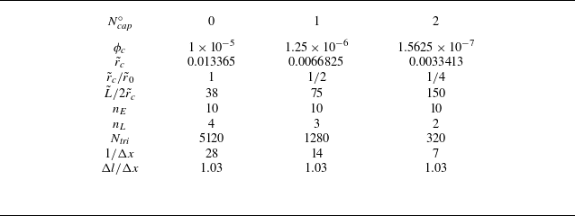


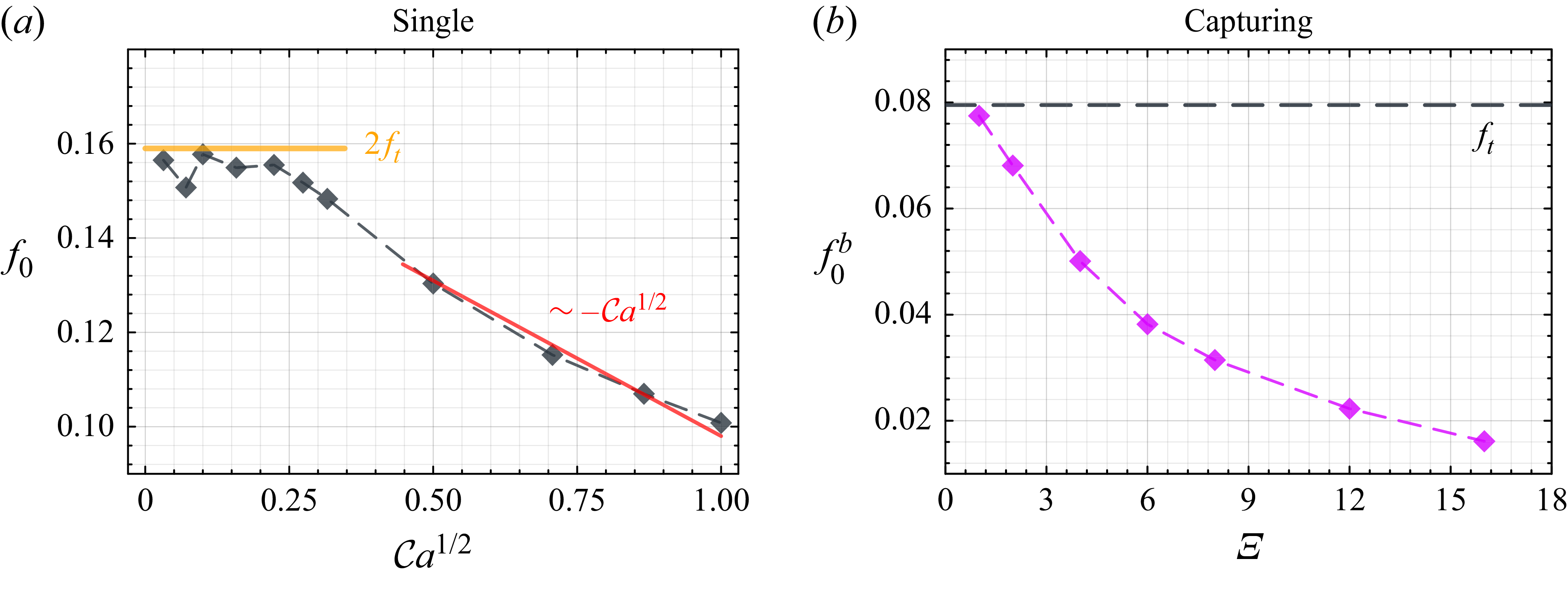


 Open access