


1. Introduction
Some of the most fundamental questions about turbulent fluid flows concern space- and time-averaged quantities, such as mean dissipation or transport, and how these quantities scale with control parameters. At parameter values that are accessible to laboratory experiments or direct numerical simulations, mean quantities can be estimated by averaging over a finite-time flow. A different and complementary approach is to mathematically derive upper or lower bounds on infinite-time averages directly from the governing equations. Most bounds of this type have been derived using the so-called background method, which was first applied to the Navier–Stokes equations by Doering & Constantin (Reference Doering and Constantin1992). For an overview of the method, see Chernyshenko (Reference Chernyshenko2022) and Fantuzzi, Arslan & Wynn (Reference Fantuzzi, Arslan and Wynn2022).
The background method lets the time-dependent governing equations be replaced by variational problems, in which integrals are maximised or minimised over time-independent velocity fields. For instance, upper bounds on infinite-time-averaged dissipation at fixed parameter values can be formulated, roughly speaking, as
 \begin{align} \text{mean dissipation} \leqslant \min _{\zeta }\max _{\boldsymbol{w}}\mathcal{Q}[\boldsymbol{w};\zeta ], \end{align}
where $\mathcal{Q}[\boldsymbol{w};\zeta ]$
is a spatial integral whose integrand depends quadratically on an incompressible velocity field
$\mathcal{Q}[\boldsymbol{w};\zeta ]$
is a spatial integral whose integrand depends quadratically on an incompressible velocity field $\boldsymbol{w}$
and linearly on a ‘background profile’
$\boldsymbol{w}$
and linearly on a ‘background profile’ $\zeta$
. In the case of lower bounds, the inner problem is a minimisation over
$\zeta$
. In the case of lower bounds, the inner problem is a minimisation over $\boldsymbol{w}$
, while the outer one is a maximisation over
$\boldsymbol{w}$
, while the outer one is a maximisation over $\zeta$
. A precise version of (1.1) for planar shear flows is derived in § 2.1.
$\zeta$
. A precise version of (1.1) for planar shear flows is derived in § 2.1.
The inner maximum in (1.1) is an upper bound on dissipation for any admissible choice of $\zeta$
. For some
$\zeta$
. For some $\zeta$
, this bound is infinity, but for other
$\zeta$
, this bound is infinity, but for other $\zeta$
, it is finite. The outer minimisation over bounds in (1.1) gives the optimal bound within the background method framework. Optimal bounds generally cannot be found analytically, but they have been computed numerically for a few fluid systems (Plasting & Kerswell Reference Plasting and Kerswell2003; Fantuzzi et al. Reference Fantuzzi, Wynn, Goulart and Papachristodoulou2017b
, Reference Fantuzzi, Pershin and Wynn2018, Reference Fantuzzi, Arslan and Wynn2022). As with direct numerical simulation of fluids, computation of optimal bounds is possible when parameters are fixed to values that are not too extreme, so that the required spatial resolution is not too fine. Most applications of the background method have instead derived suboptimal bounds analytically, which can give bounds applying at all parameter values, including with explicit parameter dependence. Such analytical results are derived by choosing relatively simple
$\zeta$
, it is finite. The outer minimisation over bounds in (1.1) gives the optimal bound within the background method framework. Optimal bounds generally cannot be found analytically, but they have been computed numerically for a few fluid systems (Plasting & Kerswell Reference Plasting and Kerswell2003; Fantuzzi et al. Reference Fantuzzi, Wynn, Goulart and Papachristodoulou2017b
, Reference Fantuzzi, Pershin and Wynn2018, Reference Fantuzzi, Arslan and Wynn2022). As with direct numerical simulation of fluids, computation of optimal bounds is possible when parameters are fixed to values that are not too extreme, so that the required spatial resolution is not too fine. Most applications of the background method have instead derived suboptimal bounds analytically, which can give bounds applying at all parameter values, including with explicit parameter dependence. Such analytical results are derived by choosing relatively simple $\zeta$
that are suboptimal, then upper-bounding the maximum over
$\zeta$
that are suboptimal, then upper-bounding the maximum over $\boldsymbol{w}$
rather than computing it exactly.
$\boldsymbol{w}$
rather than computing it exactly.
For bounds like (1.1) to hold for three-dimensional (3-D) flows, the inner maximisation generally must be over 3-D incompressible velocity fields. Maximising over a smaller class of $\boldsymbol{w}$
can make the maximum smaller and thus is not guaranteed to give an upper bound for 3-D flows. A crucial exception occurs when one can show mathematically that a maximum over 3-D velocity fields coincides with a maximum over a class of lower-dimensional velocity fields, in which case, the maximum in (1.1) need only be taken over the smaller class. This dimension reduction is significant for numerical computations of optimal bounds, which become much easier, and it may also improve analytical bounds. The present work concerns how to solve the min–max problem (1.1) over lower-dimensional velocity fields and then show a posteriori that the inner maximum would be the same over 3-D fields, thus avoiding 3-D computations.
$\boldsymbol{w}$
can make the maximum smaller and thus is not guaranteed to give an upper bound for 3-D flows. A crucial exception occurs when one can show mathematically that a maximum over 3-D velocity fields coincides with a maximum over a class of lower-dimensional velocity fields, in which case, the maximum in (1.1) need only be taken over the smaller class. This dimension reduction is significant for numerical computations of optimal bounds, which become much easier, and it may also improve analytical bounds. The present work concerns how to solve the min–max problem (1.1) over lower-dimensional velocity fields and then show a posteriori that the inner maximum would be the same over 3-D fields, thus avoiding 3-D computations.
Here, we consider planar shear flows that are bounded by two parallel walls and are periodic in the other two directions. Such flows may be sustained by boundary conditions, body forcing or both, and we assume that the governing model admits a laminar flow in a single direction. The laminar flow’s direction is called the streamwise direction, the other periodic direction is called spanwise and the bounded direction is called wall-normal. Our particular focus is on models whose governing equations are symmetric under $180^\circ$
rotation around a spanwise axis. The most prominent models in this family are plane Couette flow and any wall-bounded Kolmogorov flows with forcing profiles that are odd about the mid-plane, including the half-period sinusoidal forcing sometimes called Waleffe flow (Waleffe Reference Waleffe1997). Our main theoretical result is a criterion that applies only to shear flow models with such symmetry. In addition to fully 3-D velocity fields, we will consider fields in only the wall-normal and streamwise directions, meaning there is neither flow nor variation in the spanwise direction; these will be called two-dimensional (2-D). Fields that may be non-zero in all three components but do not vary in the streamwise direction will be called streamwise-invariant (2.5-D). Several past authors have assumed that a maximum over 2.5-D fields in (1.1) coincides with a maximum over 3-D fields. Our aim is to confirm such statements in specific cases without computing any extrema over 3-D fields.
$180^\circ$
rotation around a spanwise axis. The most prominent models in this family are plane Couette flow and any wall-bounded Kolmogorov flows with forcing profiles that are odd about the mid-plane, including the half-period sinusoidal forcing sometimes called Waleffe flow (Waleffe Reference Waleffe1997). Our main theoretical result is a criterion that applies only to shear flow models with such symmetry. In addition to fully 3-D velocity fields, we will consider fields in only the wall-normal and streamwise directions, meaning there is neither flow nor variation in the spanwise direction; these will be called two-dimensional (2-D). Fields that may be non-zero in all three components but do not vary in the streamwise direction will be called streamwise-invariant (2.5-D). Several past authors have assumed that a maximum over 2.5-D fields in (1.1) coincides with a maximum over 3-D fields. Our aim is to confirm such statements in specific cases without computing any extrema over 3-D fields.
Plane Couette flow, which is driven by parallel relative motion of the walls, has been the most-studied application of the background method to the Navier–Stokes equations. This was the first model considered by Doering & Constantin (Reference Doering and Constantin1992, Reference Doering and Constantin1994), who derived an upper bound on dissipation. Normalising the dissipation by its laminar value and by $ \textit{Re}$
gives a friction factor
$ \textit{Re}$
gives a friction factor $\varepsilon$
, for which the upper bounds become
$\varepsilon$
, for which the upper bounds become $ \textit{Re}$
-independent at large
$ \textit{Re}$
-independent at large $ \textit{Re}$
. The bound
$ \textit{Re}$
. The bound $\varepsilon \leqslant 2^{-7/2}\approx 0.0884$
of Doering & Constantin (Reference Doering and Constantin1992) is derived by choosing a simple suboptimal background profile
$\varepsilon \leqslant 2^{-7/2}\approx 0.0884$
of Doering & Constantin (Reference Doering and Constantin1992) is derived by choosing a simple suboptimal background profile $\zeta$
that depends on
$\zeta$
that depends on $ \textit{Re}$
, then using functional inequalities to upper-bound the maximum in (1.1) over 3-D
$ \textit{Re}$
, then using functional inequalities to upper-bound the maximum in (1.1) over 3-D $\boldsymbol{w}$
fields. Slightly improved analytical bounds were then derived by constructing closer-to-optimal
$\boldsymbol{w}$
fields. Slightly improved analytical bounds were then derived by constructing closer-to-optimal $\zeta$
and upper-bounding the maximum over
$\zeta$
and upper-bounding the maximum over $\boldsymbol{w}$
as sharply as possible (Gebhardt et al. Reference Gebhardt, Grossmann, Holthaus and Löhden1995). Still smaller bounds were found at various fixed
$\boldsymbol{w}$
as sharply as possible (Gebhardt et al. Reference Gebhardt, Grossmann, Holthaus and Löhden1995). Still smaller bounds were found at various fixed $ \textit{Re}$
by numerically computing the inner maxima in (1.1) and implementing the outer minimisation over a restricted class of
$ \textit{Re}$
by numerically computing the inner maxima in (1.1) and implementing the outer minimisation over a restricted class of $\zeta$
(Nicodemus, Grossmann & Holthaus Reference Nicodemus, Grossmann and Holthaus1997, Reference Nicodemus, Grossmann and Holthaus1998a
,
Reference Nicodemus, Grossmann and Holthausb
). Finally, Plasting & Kerswell (Reference Plasting and Kerswell2003) numerically carried out both the inner maximisation and the outer minimisation over the full class of
$\zeta$
(Nicodemus, Grossmann & Holthaus Reference Nicodemus, Grossmann and Holthaus1997, Reference Nicodemus, Grossmann and Holthaus1998a
,
Reference Nicodemus, Grossmann and Holthausb
). Finally, Plasting & Kerswell (Reference Plasting and Kerswell2003) numerically carried out both the inner maximisation and the outer minimisation over the full class of $\zeta$
needed, constituting the first optimal bounds of the background method for any fluid flow. Their computed bounds on
$\zeta$
needed, constituting the first optimal bounds of the background method for any fluid flow. Their computed bounds on $\varepsilon$
approach a constant near 0.008553 as
$\varepsilon$
approach a constant near 0.008553 as $ \textit{Re}\to \infty$
, which remains the best known bound on dissipation for plane Couette flow. However, the analyses of Plasting & Kerswell (Reference Plasting and Kerswell2003) and Nicodemus et al. (Reference Nicodemus, Grossmann and Holthaus1998a
,Reference Nicodemus, Grossmann and Holthaus
b
) are not quite complete. In their computations, inner maximisation in (1.1) was generally carried out only over 2.5-D
$ \textit{Re}\to \infty$
, which remains the best known bound on dissipation for plane Couette flow. However, the analyses of Plasting & Kerswell (Reference Plasting and Kerswell2003) and Nicodemus et al. (Reference Nicodemus, Grossmann and Holthaus1998a
,Reference Nicodemus, Grossmann and Holthaus
b
) are not quite complete. In their computations, inner maximisation in (1.1) was generally carried out only over 2.5-D $\boldsymbol{w}$
fields. If this maximum is smaller than the maximum over 3-D
$\boldsymbol{w}$
fields. If this maximum is smaller than the maximum over 3-D $\boldsymbol{w}$
, then it need not be a bound for 3-D flows. (A bound for 2.5-D flows alone is not needed since all 2.5-D flows decay to the laminar state, as follows from energy stability analysis using only streamwise and wall-normal velocity components.) These authors maximised only over 2.5-D
$\boldsymbol{w}$
, then it need not be a bound for 3-D flows. (A bound for 2.5-D flows alone is not needed since all 2.5-D flows decay to the laminar state, as follows from energy stability analysis using only streamwise and wall-normal velocity components.) These authors maximised only over 2.5-D $\boldsymbol{w}$
because they conjectured that the maximum over fully 3-D
$\boldsymbol{w}$
because they conjectured that the maximum over fully 3-D $\boldsymbol{w}$
would give the same value. Plasting & Kerswell (personal communication) and Nicodemus et al. (Reference Nicodemus, Grossmann and Holthaus1997) confirmed this conjecture at a few modest parameter values by carrying out 3-D computations, but they did not show it to be true in general.
$\boldsymbol{w}$
would give the same value. Plasting & Kerswell (personal communication) and Nicodemus et al. (Reference Nicodemus, Grossmann and Holthaus1997) confirmed this conjecture at a few modest parameter values by carrying out 3-D computations, but they did not show it to be true in general.
We derive a criterion for shear flow models that, when it holds, implies coincidence of maxima in (1.1) over 2.5-D fields and over 3-D fields, and likewise for minima in the case of lower bounds. This criterion applies if the governing model has $180^\circ$
rotational symmetry, but the flow need not be symmetric. We rely on a theorem of Busse (Reference Busse1972) for energy stability of models with the rotational symmetry. Checking our criterion does not require extremising over 3-D fields. Instead, at fixed parameters, one must find the extremum of
$180^\circ$
rotational symmetry, but the flow need not be symmetric. We rely on a theorem of Busse (Reference Busse1972) for energy stability of models with the rotational symmetry. Checking our criterion does not require extremising over 3-D fields. Instead, at fixed parameters, one must find the extremum of $\mathcal{Q}$
and a related functional over 2.5-D fields, extremise another related functional over 2-D fields and then check whether a ratio involving these three extrema is less than unity. In computational examples, the ratio asymptotes to a constant as
$\mathcal{Q}$
and a related functional over 2.5-D fields, extremise another related functional over 2-D fields and then check whether a ratio involving these three extrema is less than unity. In computational examples, the ratio asymptotes to a constant as $ \textit{Re}\to \infty$
. If the asymptote is less than unity, this gives strong evidence that the coincidence of 2.5-D and 3-D extrema can be ‘extrapolated’ to all
$ \textit{Re}\to \infty$
. If the asymptote is less than unity, this gives strong evidence that the coincidence of 2.5-D and 3-D extrema can be ‘extrapolated’ to all $ \textit{Re}$
.
$ \textit{Re}$
.
When our criterion is not useful because it is either false or inapplicable, one can instead check directly that maximisers in (1.1) are 2.5-D. As explained later, the min–max problem (1.1) can be rewritten as a minimisation subject to a so-called spectral constraint, which requires all eigenvalues of a certain linear eigenproblem to be non-negative. This eigenproblem depends on the background profile $\zeta$
and can be solved independently for each pair of the streamwise and spanwise wavenumbers. After solving (1.1) over 2.5-D
$\zeta$
and can be solved independently for each pair of the streamwise and spanwise wavenumbers. After solving (1.1) over 2.5-D $\boldsymbol{w}$
and finding the optimal
$\boldsymbol{w}$
and finding the optimal $\zeta$
, one can check a posteriori that no 3-D fields violate the spectral constraint – that is, one can check the eigenvalues for non-zero streamwise wavenumbers.
$\zeta$
, one can check a posteriori that no 3-D fields violate the spectral constraint – that is, one can check the eigenvalues for non-zero streamwise wavenumbers.
Here, we compute optimal background method bounds on dissipation for both Waleffe flow and Couette flow. In Waleffe flow, dissipation is maximised by the laminar state, so only lower bounds must be computed. In Couette flow, the situation is reversed and only upper bounds must be computed. For both flows, we fix streamwise and spanwise periods of the domain and solve (1.1) computationally up to moderate $ \textit{Re}$
values over 2.5-D fields, then we verify that the maxima over 3-D fields would coincide. In the case of Waleffe flow, the ratio used in our criterion asymptotes to a value well below unity, suggesting that (1.1) will coincide for 2.5-D and 3-D fields at all
$ \textit{Re}$
values over 2.5-D fields, then we verify that the maxima over 3-D fields would coincide. In the case of Waleffe flow, the ratio used in our criterion asymptotes to a value well below unity, suggesting that (1.1) will coincide for 2.5-D and 3-D fields at all $ \textit{Re}$
values. In the case of Couette flow, our computations roughly reproduce those of Plasting & Kerswell (Reference Plasting and Kerswell2003), but up to smaller
$ \textit{Re}$
values. In the case of Couette flow, our computations roughly reproduce those of Plasting & Kerswell (Reference Plasting and Kerswell2003), but up to smaller $ \textit{Re}$
and with the spatial periods fixed. The ratio used in our criterion exceeds unity if
$ \textit{Re}$
and with the spatial periods fixed. The ratio used in our criterion exceeds unity if $ \textit{Re}\gtrsim 254$
, so it cannot validate the assumption of Plasting & Kerswell that maximisers are 2.5-D at all
$ \textit{Re}\gtrsim 254$
, so it cannot validate the assumption of Plasting & Kerswell that maximisers are 2.5-D at all $ \textit{Re}$
. Instead, we directly check that the spectral constraint holds for 3-D fields over our modest
$ \textit{Re}$
. Instead, we directly check that the spectral constraint holds for 3-D fields over our modest $ \textit{Re}$
range, which it does. To the extent that this spectrum can be extrapolated, it is consistent with the assumption of Plasting & Kerswell. Additionally, we repeat the bounding computations for Couette flow with further constraints on
$ \textit{Re}$
range, which it does. To the extent that this spectrum can be extrapolated, it is consistent with the assumption of Plasting & Kerswell. Additionally, we repeat the bounding computations for Couette flow with further constraints on $\zeta$
that guarantee our criterion will be satisfied, giving bounds for 3-D flows that extrapolate to large
$\zeta$
that guarantee our criterion will be satisfied, giving bounds for 3-D flows that extrapolate to large $ \textit{Re}$
with a prefactor slightly worse than that of Plasting & Kerswell.
$ \textit{Re}$
with a prefactor slightly worse than that of Plasting & Kerswell.
This article is organised as follows. Section 2 formulates the background method for planar parallel shear flows, including three equivalent reformulations with the spectral constraint. Section 3 derives our criterion for extrema over 2.5-D and 3-D fields to coincide in models with $180^\circ$
rotational symmetry. Section 4 presents our computational applications to Waleffe flow and Couette flow, followed by conclusions in § 5. Appendices A–C provide details of certain arguments and computations, as well as an exposition of the proof of Busse (Reference Busse1972) that underlies our own criterion.
$180^\circ$
rotational symmetry. Section 4 presents our computational applications to Waleffe flow and Couette flow, followed by conclusions in § 5. Appendices A–C provide details of certain arguments and computations, as well as an exposition of the proof of Busse (Reference Busse1972) that underlies our own criterion.
2. Four formulations of the background method for planar shear flows
We consider an incompressible fluid flow bounded by two planar walls located at dimensionless coordinates $z=-1/2$
and
$z=-1/2$
and $z=1/2$
, where lengths have been scaled by the distance
$z=1/2$
, where lengths have been scaled by the distance $d$
between the walls. Body forcing of the fluid and/or relative motion of the boundaries is assumed to point in only the
$d$
between the walls. Body forcing of the fluid and/or relative motion of the boundaries is assumed to point in only the $x$
direction, so that there exists a laminar flow in that direction. In the nomenclature of shear flows, the
$x$
direction, so that there exists a laminar flow in that direction. In the nomenclature of shear flows, the $x$
direction is streamwise,
$x$
direction is streamwise, $y$
is spanwise and
$y$
is spanwise and $z$
is wall-normal. We assume the flow is periodic in the streamwise and spanwise directions with dimensionless periods of
$z$
is wall-normal. We assume the flow is periodic in the streamwise and spanwise directions with dimensionless periods of $\varGamma _x$
and
$\varGamma _x$
and $\varGamma _y$
, respectively, so we let
$\varGamma _y$
, respectively, so we let $-\varGamma _x/2\leqslant x\leqslant \varGamma _x/2$
and
$-\varGamma _x/2\leqslant x\leqslant \varGamma _x/2$
and $-\varGamma _y/2\leqslant y\leqslant \varGamma _y/2$
. The Navier–Stokes equations governing the dimensionless velocity vector
$-\varGamma _y/2\leqslant y\leqslant \varGamma _y/2$
. The Navier–Stokes equations governing the dimensionless velocity vector $\boldsymbol{u}(\boldsymbol{x},t)$
and pressure
$\boldsymbol{u}(\boldsymbol{x},t)$
and pressure $p(\boldsymbol{x},t)$
are
$p(\boldsymbol{x},t)$
are
 \begin{align} \partial _t\boldsymbol{u}+\boldsymbol{u}\boldsymbol{\cdot }\boldsymbol{\nabla }\boldsymbol{u}=-\boldsymbol{\nabla }p+\frac {1}{\textit{Re}}{\nabla} ^2\boldsymbol{u} + f\hat {\boldsymbol{x}}, \quad \boldsymbol{\nabla }\boldsymbol{\cdot }\boldsymbol{u}=0, \end{align}
where $ \textit{Re}={d}\mathsf{U}/\nu$
is the Reynolds number,
$ \textit{Re}={d}\mathsf{U}/\nu$
is the Reynolds number, $\nu$
is the kinematic viscosity,
$\nu$
is the kinematic viscosity, $\mathsf{U}$
is a dimensional velocity defined either using the boundary conditions or body forcing and time has been scaled by
$\mathsf{U}$
is a dimensional velocity defined either using the boundary conditions or body forcing and time has been scaled by $d^2/\nu$
. If there is body forcing, it is in the streamwise direction
$d^2/\nu$
. If there is body forcing, it is in the streamwise direction $\hat {\boldsymbol{x}}$
and varies only in the wall-normal direction, so it takes the form
$\hat {\boldsymbol{x}}$
and varies only in the wall-normal direction, so it takes the form $f(z)\hat {\boldsymbol{x}}$
. The walls are impenetrable, meaning the wall-normal velocity
$f(z)\hat {\boldsymbol{x}}$
. The walls are impenetrable, meaning the wall-normal velocity $\boldsymbol{u}\boldsymbol{\cdot }\hat {\boldsymbol{z}}$
vanishes, and remaining boundary conditions fix the tangential components of either the velocity vector
$\boldsymbol{u}\boldsymbol{\cdot }\hat {\boldsymbol{z}}$
vanishes, and remaining boundary conditions fix the tangential components of either the velocity vector $\boldsymbol{u}$
or the stresses
$\boldsymbol{u}$
or the stresses $\partial _z\boldsymbol{u}$
. In the fixed-velocity case, the boundary conditions are
$\partial _z\boldsymbol{u}$
. In the fixed-velocity case, the boundary conditions are
 \begin{align} u_1=C,\quad u_2=0,\quad u_3=0\quad \text{at}\quad z=\pm \frac 12, \end{align}
and in the fixed-stress case, they are
 \begin{align} \partial _z u_1=C,\quad \partial _z u_2=0,\quad u_3 = 0 \quad \text{at}\quad z=\pm \frac 12, \end{align}
where $C$
can be any constant (including zero) and can be different at each boundary.
$C$
can be any constant (including zero) and can be different at each boundary.
The configurations described previously admit a laminar solution $U(z)\hat {\boldsymbol{x}}$
to the governing equations (2.1). Most derivations here are done in terms of the deviation
$U(z)\hat {\boldsymbol{x}}$
to the governing equations (2.1). Most derivations here are done in terms of the deviation $\boldsymbol{v}$
from the laminar state, which is defined by
$\boldsymbol{v}$
from the laminar state, which is defined by $\boldsymbol{u}(\boldsymbol{x},t)=U(z)\boldsymbol{\hat {x}}+\boldsymbol{v}(\boldsymbol{x},t)$
. Denoting the components of the deviation by
$\boldsymbol{u}(\boldsymbol{x},t)=U(z)\boldsymbol{\hat {x}}+\boldsymbol{v}(\boldsymbol{x},t)$
. Denoting the components of the deviation by $\boldsymbol{v}=(v_1,v_2,v_3)$
, the evolution of
$\boldsymbol{v}=(v_1,v_2,v_3)$
, the evolution of $\boldsymbol{v}$
implied by (2.1) is
$\boldsymbol{v}$
implied by (2.1) is
 \begin{align} \partial _t\boldsymbol{v} + \boldsymbol{v}\boldsymbol{\cdot }\boldsymbol{\nabla }\boldsymbol{v} + U\partial _x\boldsymbol{v} + U^{\prime}v_3\hat {\boldsymbol{x}} =- \boldsymbol{\nabla }p + \frac {1}{\textit{Re}}{\nabla} ^2\boldsymbol{v},\quad \boldsymbol{\nabla }\boldsymbol{\cdot }\boldsymbol{v}=0, \end{align}
where primes denote ordinary derivatives in $z$
. Boundary conditions on the deviation
$z$
. Boundary conditions on the deviation $\boldsymbol{v}$
are homogeneous. At a boundary where
$\boldsymbol{v}$
are homogeneous. At a boundary where $\boldsymbol{u}$
satisfies the fixed-velocity condition (2.2), the
$\boldsymbol{u}$
satisfies the fixed-velocity condition (2.2), the $\boldsymbol{v}$
condition is no-slip,
$\boldsymbol{v}$
condition is no-slip,
 \begin{align} \boldsymbol{v}=\boldsymbol{0}\quad \text{at}\quad z=\pm \frac 12. \end{align}
At a boundary where $\boldsymbol{u}$
satisfies the fixed-stress condition (2.3), the
$\boldsymbol{u}$
satisfies the fixed-stress condition (2.3), the $\boldsymbol{v}$
condition is stress-free,
$\boldsymbol{v}$
condition is stress-free,
 \begin{align} \partial _z v_1=\partial _z v_2=v_3 = 0 \quad \text{at}\quad z=\pm \frac 12. \end{align}
Formulations of the background method in the present section assume that (2.5) or (2.6) holds at each boundary, but the two boundaries need not be the same. Results in § 3 require the same condition at both boundaries.
2.1. Background method formulation in terms of auxiliary functionals
For shear flows governed by (2.1), the quantity that has most often been bounded using the background method is the mean dissipation. We let angle brackets denote an average over the spatial domain $\varOmega$
and let an overbar denote an infinite-time average, so the dimensionless dissipation averaged over the volume and infinite time is
$\varOmega$
and let an overbar denote an infinite-time average, so the dimensionless dissipation averaged over the volume and infinite time is
 \begin{align} \overline {\big \langle |\boldsymbol{\nabla }\boldsymbol{u}|^2\big \rangle }=\lim _{T\to \infty }\frac {1}{T}\int _0^T\frac {1}{\varGamma _x\varGamma _y}\int _{\varOmega }|\boldsymbol{\nabla }\boldsymbol{u}|^2\,{\mathrm{d}}\boldsymbol{x}\,{\mathrm{d}}t, \end{align}
where $\varGamma _x\varGamma _y$
is the volume of the dimensionless domain and, if the infinite-time limit is not well defined, one can take the limit supremum. The dimensionless quantity (2.7) is the same one used in previous works such as that of Plasting & Kerswell (Reference Plasting and Kerswell2003). For physical interpretation in § 4, we examine this dissipation’s ratio to its laminar value since this ratio does not depend on the chosen non-dimensionalisation. The average dissipation is related a priori to the average rate of energy input by body and boundary forces, as explained for the examples of Wallefe flow and Couette flow in § 4.
$\varGamma _x\varGamma _y$
is the volume of the dimensionless domain and, if the infinite-time limit is not well defined, one can take the limit supremum. The dimensionless quantity (2.7) is the same one used in previous works such as that of Plasting & Kerswell (Reference Plasting and Kerswell2003). For physical interpretation in § 4, we examine this dissipation’s ratio to its laminar value since this ratio does not depend on the chosen non-dimensionalisation. The average dissipation is related a priori to the average rate of energy input by body and boundary forces, as explained for the examples of Wallefe flow and Couette flow in § 4.
Whether one seeks upper or lower bounds depends on the model. Often, it is easy to show that the dissipation among all flows is bounded below or above by the laminar dissipation, in which case, it remains only to find upper or lower bounds, respectively. For concreteness, our exposition in this section considers upper bounds on mean dissipation. Section 2.4 summarises what changes in the case of lower bounds. The background method can bound averages of other linear or quadratic integrals also, such as kinetic energy, by straightforward modifications to the formulations given here.
Our goal is to derive bounds on (2.7) that apply to all solutions of the governing equations (2.1) subject to boundary conditions, regardless of the initial conditions. We give the derivation in terms of a so-called auxiliary functional $V$
. Such functionals have not been explicitly used in the background method literature until recently, but they are implicit in all such arguments, as explained by Chernyshenko (Reference Chernyshenko2022) and Fantuzzi et al. (Reference Fantuzzi, Arslan and Wynn2022). An auxiliary functional
$V$
. Such functionals have not been explicitly used in the background method literature until recently, but they are implicit in all such arguments, as explained by Chernyshenko (Reference Chernyshenko2022) and Fantuzzi et al. (Reference Fantuzzi, Arslan and Wynn2022). An auxiliary functional $V[\boldsymbol{w}]$
maps a divergence-free, time-independent vector field
$V[\boldsymbol{w}]$
maps a divergence-free, time-independent vector field $\boldsymbol{w}(\boldsymbol{x})$
to a real number. All past applications of the background method to planar shear flows are equivalent to choosing
$\boldsymbol{w}(\boldsymbol{x})$
to a real number. All past applications of the background method to planar shear flows are equivalent to choosing $V[\boldsymbol{w}]$
that is a quadratic spatial integral of the form
$V[\boldsymbol{w}]$
that is a quadratic spatial integral of the form
 \begin{align} V[\boldsymbol{w}]=\textit{Re}\left \langle \frac {a}{2}|\boldsymbol{w}|^2- \zeta \hat {\boldsymbol{x}}\boldsymbol{\cdot }\boldsymbol{w}\right \rangle \! , \end{align}
where the functional is defined by choosing the ‘balance parameter’ $a$
and the ‘background field’
$a$
and the ‘background field’ $\zeta (z)\hat {\boldsymbol{x}}$
. The quantity
$\zeta (z)\hat {\boldsymbol{x}}$
. The quantity $({1}/{a})\zeta$
is called the background field in the notation of most prior works (cf. Chernyshenko Reference Chernyshenko2022), but it is useful for what follows to define notation for
$({1}/{a})\zeta$
is called the background field in the notation of most prior works (cf. Chernyshenko Reference Chernyshenko2022), but it is useful for what follows to define notation for $\zeta$
rather than for
$\zeta$
rather than for $({1}/{a})\zeta$
because then,
$({1}/{a})\zeta$
because then, $a$
and
$a$
and $\zeta$
appear linearly in
$\zeta$
appear linearly in $V$
. Generalisations of (2.8) that go beyond quadratic integrals have the potential to give stronger results, as they do for the Kuramoto–Sivashinsky equation (Goluskin & Fantuzzi Reference Goluskin and Fantuzzi2019), but the present work concerns the background method and thus only
$V$
. Generalisations of (2.8) that go beyond quadratic integrals have the potential to give stronger results, as they do for the Kuramoto–Sivashinsky equation (Goluskin & Fantuzzi Reference Goluskin and Fantuzzi2019), but the present work concerns the background method and thus only $V$
of the form (2.8). There is no advantage to considering a background field of more general form than
$V$
of the form (2.8). There is no advantage to considering a background field of more general form than $\zeta (z)\hat {\boldsymbol{x}}$
, as proved in Appendix A.1 using symmetry arguments. To enable integration by parts later, the background field is admissible only if it is continuous and piecewise smooth, and if it satisfies the same boundary conditions as
$\zeta (z)\hat {\boldsymbol{x}}$
, as proved in Appendix A.1 using symmetry arguments. To enable integration by parts later, the background field is admissible only if it is continuous and piecewise smooth, and if it satisfies the same boundary conditions as $\boldsymbol{v}(\boldsymbol{x},t)$
.
$\boldsymbol{v}(\boldsymbol{x},t)$
.
The definition of $V$
does not involve time, but one obtains a scalar-valued function of time by considering
$V$
does not involve time, but one obtains a scalar-valued function of time by considering $V[\boldsymbol{v}(\boldsymbol{x},t)]$
, where
$V[\boldsymbol{v}(\boldsymbol{x},t)]$
, where $\boldsymbol{v}$
solves (2.4). For choices of
$\boldsymbol{v}$
solves (2.4). For choices of $V$
that lead to finite bounds on mean dissipation, it can be shown that
$V$
that lead to finite bounds on mean dissipation, it can be shown that $V[\boldsymbol{v}(\boldsymbol{x},t)]$
remains bounded as
$V[\boldsymbol{v}(\boldsymbol{x},t)]$
remains bounded as $t\to \infty$
for any admissible initial condition
$t\to \infty$
for any admissible initial condition $\boldsymbol{v}(\boldsymbol{x},0)$
(Doering & Constantin Reference Doering and Constantin1994). All such
$\boldsymbol{v}(\boldsymbol{x},0)$
(Doering & Constantin Reference Doering and Constantin1994). All such $V$
satisfy the identity
$V$
satisfy the identity
 \begin{align} \overline {\frac {\mathrm{d}}{{\mathrm{d}}t}V[\boldsymbol{v}(\boldsymbol{x},t)]}=\lim _{T\to \infty }\frac {1}{T}\left (V[\boldsymbol{v}(\boldsymbol{x},T)]-V[\boldsymbol{v}(\boldsymbol{x},0)]\right )=0, \end{align}
so the time-averaged dissipation $\overline {\langle |\boldsymbol{\nabla }\boldsymbol{u}|^2\rangle }$
that we want to bound is equal to
$\overline {\langle |\boldsymbol{\nabla }\boldsymbol{u}|^2\rangle }$
that we want to bound is equal to $\overline {\langle |\boldsymbol{\nabla }\boldsymbol{u}|^2\rangle +({\mathrm{d}}/{{\mathrm{d}}t})V}$
. Moreover, one can find an expression equal to
$\overline {\langle |\boldsymbol{\nabla }\boldsymbol{u}|^2\rangle +({\mathrm{d}}/{{\mathrm{d}}t})V}$
. Moreover, one can find an expression equal to $({\mathrm{d}}/{{\mathrm{d}}t})V[\boldsymbol{v}]$
without explicit time-dependence:
$({\mathrm{d}}/{{\mathrm{d}}t})V[\boldsymbol{v}]$
without explicit time-dependence:
 \begin{align} \frac {\mathrm{d}}{{\mathrm{d}}t}V[\boldsymbol{v}(\boldsymbol{x},t)] &= \textit{Re}\left \langle (a\boldsymbol{v}-\zeta \hat {\boldsymbol{x}})\boldsymbol{\cdot }\partial _t\boldsymbol{v}\right \rangle \\[-10pt] \nonumber \end{align}
 \begin{align} &=\textit{Re}\left \langle (a\boldsymbol{v}-\zeta \hat {\boldsymbol{x}})\boldsymbol{\cdot }\left ( {-}\boldsymbol{v}\boldsymbol{\cdot }\boldsymbol{\nabla }\boldsymbol{v} - U\partial _x\boldsymbol{v} - U^{\prime}v_3\hat {\boldsymbol{x}} -\boldsymbol{\nabla }p + \frac {1}{\textit{Re}}{\nabla} ^2\boldsymbol{v} \right )\right \rangle \\[-10pt] \nonumber \end{align}
 \begin{align} &= \big \langle {-}a|\boldsymbol{\nabla }\boldsymbol{v}|^2+\zeta^{\prime}\partial _zv_1-\textit{Re}\left (aU+\zeta \right )^{\prime}v_1v_3\big \rangle . \\[9pt] \nonumber\end{align}
Equation (2.10) is derived by moving the time derivative inside the volume integral, and (2.11) replaces $\partial _t\boldsymbol{v}$
according to (2.4). Equation (2.12) follows from integration by parts, recalling that we require
$\partial _t\boldsymbol{v}$
according to (2.4). Equation (2.12) follows from integration by parts, recalling that we require $\zeta (z)\hat {\boldsymbol{x}}$
to satisfy the same boundary conditions as
$\zeta (z)\hat {\boldsymbol{x}}$
to satisfy the same boundary conditions as $\boldsymbol{v}$
, which may be stress-free or no-slip at each boundary. Finally, we find a useful expression with the same time average as the dissipation:
$\boldsymbol{v}$
, which may be stress-free or no-slip at each boundary. Finally, we find a useful expression with the same time average as the dissipation:
 \begin{align} \overline {\langle |\boldsymbol{\nabla }\boldsymbol{u}|^2\rangle } &=\overline {\big \langle {U}^{\prime2}+2U^{\prime}\partial _zv_1+|\boldsymbol{\nabla }\boldsymbol{v}|^2 \big\rangle } \\[-10pt] \nonumber \end{align}
 \begin{align} &= \overline {\big\langle {U}^{\prime2}+2U^{\prime}\partial _zv_1+|\boldsymbol{\nabla }\boldsymbol{v}|^2 \big\rangle +\frac {\textrm{d}}{\textrm{d}t}V[\boldsymbol{v}(\boldsymbol{x},t)]} \\[-10pt] \nonumber \end{align}
 \begin{align} &= \overline {\mathcal{Q}[\boldsymbol{v}(\boldsymbol{x},t)]}, \\[9pt] \nonumber \end{align}
where the functional $\mathcal{Q}$
is defined as
$\mathcal{Q}$
is defined as
 \begin{align} \mathcal{Q}[\boldsymbol{w}]=\big \langle {U}^{\prime2}+(2U+\zeta )^{\prime}\partial _zw_1-(a-1)|\boldsymbol{\nabla }\boldsymbol{w}|^2-\textit{Re}(aU+\zeta )^{\prime}w_1w_3\big \rangle \end{align}
for any time-independent, divergence-free vector field $\boldsymbol{w}=(w_1,w_2,w_3)$
that obeys the same boundary conditions as
$\boldsymbol{w}=(w_1,w_2,w_3)$
that obeys the same boundary conditions as $\boldsymbol{v}$
. The equality (2.13) follows from substituting
$\boldsymbol{v}$
. The equality (2.13) follows from substituting $\boldsymbol{u}=U\hat {\boldsymbol{x}}+\boldsymbol{v}$
, the next equality uses (2.9), and then applying (2.12) gives the expression for
$\boldsymbol{u}=U\hat {\boldsymbol{x}}+\boldsymbol{v}$
, the next equality uses (2.9), and then applying (2.12) gives the expression for $\mathcal{Q}[\boldsymbol{w}]$
.
$\mathcal{Q}[\boldsymbol{w}]$
.
Since the time average $\overline {\mathcal{Q}[\boldsymbol{v}]}$
is bounded above by the maximum of
$\overline {\mathcal{Q}[\boldsymbol{v}]}$
is bounded above by the maximum of $\mathcal{Q}[\boldsymbol{w}]$
over all possible
$\mathcal{Q}[\boldsymbol{w}]$
over all possible $\boldsymbol{w}$
, (2.15) implies
$\boldsymbol{w}$
, (2.15) implies
 \begin{align} \overline {\big\langle |\boldsymbol{\nabla }\boldsymbol{u}|^2 \big\rangle } \leqslant \max _{\boldsymbol{w}\in \mathcal{H}_{3D}}\mathcal{Q}[\boldsymbol{w}] \end{align}
for any $a$
and any admissible
$a$
and any admissible $\zeta$
, where
$\zeta$
, where $\mathcal{H}_{3D}$
is the class of 3-D divergence-free vector fields
$\mathcal{H}_{3D}$
is the class of 3-D divergence-free vector fields $\boldsymbol{w}(\boldsymbol{x})$
that satisfy the same boundary conditions (2.5) or (2.6) as
$\boldsymbol{w}(\boldsymbol{x})$
that satisfy the same boundary conditions (2.5) or (2.6) as $\boldsymbol{v}(\boldsymbol{x},t)$
does. The right-hand maximum in (2.17) can be finite or infinite, depending on
$\boldsymbol{v}(\boldsymbol{x},t)$
does. The right-hand maximum in (2.17) can be finite or infinite, depending on $a$
and
$a$
and $\zeta$
. When the maximum is finite, it can be computed numerically or bounded above analytically. One naturally wants to choose
$\zeta$
. When the maximum is finite, it can be computed numerically or bounded above analytically. One naturally wants to choose $a$
and
$a$
and $\zeta$
to make the resulting upper bound as small as possible. At each fixed
$\zeta$
to make the resulting upper bound as small as possible. At each fixed $ \textit{Re}$
, the upper bound on dissipation that is optimal within the framework of the background method is the solution to a min–max problem,
$ \textit{Re}$
, the upper bound on dissipation that is optimal within the framework of the background method is the solution to a min–max problem,
 \begin{align} \overline {\big \langle |\boldsymbol{\nabla }\boldsymbol{u}|^2\big \rangle }\leqslant \min _{\substack {a,\,\zeta }}\max _{\boldsymbol{w}\in \mathcal{H}_{3\text{D}}}\mathcal{Q}[\boldsymbol{w}], \end{align}
where the function class over which $\zeta$
is minimised is such that
$\zeta$
is minimised is such that $\zeta \hat {\boldsymbol{x}}\in \mathcal{H}_{3\text{D}}$
. In §§ 2.2 and 2.3, we give three more formulations that are equivalent to (2.18) and are useful for different purposes.
$\zeta \hat {\boldsymbol{x}}\in \mathcal{H}_{3\text{D}}$
. In §§ 2.2 and 2.3, we give three more formulations that are equivalent to (2.18) and are useful for different purposes.
The optimal background method formulation (2.18) is a more precise version of (1.1) for the case of planar shear flows. Since the inner maximisation gives an infinite value for some $a$
and
$a$
and $\zeta$
, strictly speaking, the minimum and maximum should be called an infimum and supremum, respectively, but we use the notation
$\zeta$
, strictly speaking, the minimum and maximum should be called an infimum and supremum, respectively, but we use the notation $\min$
and
$\min$
and $\max$
throughout. Provided these values are finite, we assume that all maxima and minima are attained, meaning that there exist
$\max$
throughout. Provided these values are finite, we assume that all maxima and minima are attained, meaning that there exist $a$
,
$a$
, $\zeta$
and
$\zeta$
and $\boldsymbol{w}$
for which
$\boldsymbol{w}$
for which $\mathcal{Q}[\boldsymbol{w}]$
is equal to its min–max in (2.18). Such attainment relies on optimising
$\mathcal{Q}[\boldsymbol{w}]$
is equal to its min–max in (2.18). Such attainment relies on optimising $\zeta$
and
$\zeta$
and $\boldsymbol{w}$
over sufficiently large function spaces (Evans Reference Evans2022), but the exact choice of these spaces is beyond our scope.
$\boldsymbol{w}$
over sufficiently large function spaces (Evans Reference Evans2022), but the exact choice of these spaces is beyond our scope.
2.2.
Mean and mean-free decomposition of $\mathcal{Q}$

The maximisation over $\boldsymbol{w}$
in (2.17) can be decoupled into maximisations over the planar mean of
$\boldsymbol{w}$
in (2.17) can be decoupled into maximisations over the planar mean of $\boldsymbol{w}$
and over its remaining mean-free part. This decoupling leads to a variational problem familiar from energy stability analysis, eventually allowing us to apply the theorem of Busse (Reference Busse1972). It also reveals that finite values of the upper bound (2.17) depend on
$\boldsymbol{w}$
and over its remaining mean-free part. This decoupling leads to a variational problem familiar from energy stability analysis, eventually allowing us to apply the theorem of Busse (Reference Busse1972). It also reveals that finite values of the upper bound (2.17) depend on $a$
and
$a$
and $\zeta$
, but not on
$\zeta$
, but not on $ \textit{Re}$
, even though the functional
$ \textit{Re}$
, even though the functional $\mathcal{Q}$
being maximised depends also on
$\mathcal{Q}$
being maximised depends also on $ \textit{Re}$
. For fixed
$ \textit{Re}$
. For fixed $a$
and
$a$
and $\zeta$
, the maximum will assume a constant value at sufficiently small
$\zeta$
, the maximum will assume a constant value at sufficiently small $ \textit{Re}$
, and for larger
$ \textit{Re}$
, and for larger $ \textit{Re}$
, the right-hand side of (2.17) will be infinite.
$ \textit{Re}$
, the right-hand side of (2.17) will be infinite.
We decompose the divergence-free vector field $\boldsymbol{w}$
as
$\boldsymbol{w}$
as
 \begin{align} \boldsymbol{w}(\boldsymbol{x})=\boldsymbol{F}(z)+\dot {\boldsymbol{w}}(\boldsymbol{x}), \end{align}
where $\boldsymbol{F}$
is the mean of
$\boldsymbol{F}$
is the mean of $\boldsymbol{w}$
over the periodic
$\boldsymbol{w}$
over the periodic $x$
and
$x$
and $y$
directions, and
$y$
directions, and $\dot {\boldsymbol{w}}$
is the remaining mean-free part. We denote the components of the mean as
$\dot {\boldsymbol{w}}$
is the remaining mean-free part. We denote the components of the mean as $\boldsymbol{F}=(F_1,F_2,0)$
, where the zero wall-normal component follows from impenetrability of the walls and incompressibility. With
$\boldsymbol{F}=(F_1,F_2,0)$
, where the zero wall-normal component follows from impenetrability of the walls and incompressibility. With $\boldsymbol{w}$
so decomposed, the
$\boldsymbol{w}$
so decomposed, the $\mathcal{Q}$
functional defined by (2.16) decouples into functionals of
$\mathcal{Q}$
functional defined by (2.16) decouples into functionals of $\boldsymbol{F}$
and of
$\boldsymbol{F}$
and of $\dot {\boldsymbol{w}}$
,
$\dot {\boldsymbol{w}}$
,
 \begin{align} \mathcal{Q}[\boldsymbol{F}+\dot {\boldsymbol{w}}]=\big \langle {U}^{\prime2}\big \rangle +\mathcal{F}[\boldsymbol{F}]+\mathcal{E}[\dot {\boldsymbol{w}}], \end{align}
where
 \begin{align} \mathcal{F}[\boldsymbol{F}] &= \big \langle (2U+\zeta )^{\prime}F^{\prime}_1-(a-1)\big ({F^{\prime2}_1}+{F^{\prime2}_2}\big )\big \rangle , \\[-10pt] \nonumber \end{align}
 \begin{align} \mathcal{E}[\dot {\boldsymbol{w}}] &= \big \langle -(a-1)|\boldsymbol{\nabla }\dot {\boldsymbol{w}}|^2-\textit{Re}\,(aU+\zeta )^{\prime}\dot {w}_1\dot {w}_3\big \rangle . \\[9pt] \nonumber \end{align}
To find the maximum of $\mathcal{Q}[\boldsymbol{w}]$
, we can separately maximise
$\mathcal{Q}[\boldsymbol{w}]$
, we can separately maximise $\mathcal{F}[\boldsymbol{F}]$
and
$\mathcal{F}[\boldsymbol{F}]$
and $\mathcal{E}[\dot {\boldsymbol{w}}]$
.
$\mathcal{E}[\dot {\boldsymbol{w}}]$
.
The functional $\mathcal{F}[\boldsymbol{F}]$
has a finite maximum only if
$\mathcal{F}[\boldsymbol{F}]$
has a finite maximum only if $a\gt 1$
, so we assume this hereafter. Since the
$a\gt 1$
, so we assume this hereafter. Since the $F_2$
term in (2.21) is non-positive and independent of other terms, the maximiser
$F_2$
term in (2.21) is non-positive and independent of other terms, the maximiser $\boldsymbol{F}^*$
that attains the maximum of
$\boldsymbol{F}^*$
that attains the maximum of $\mathcal{F}$
must have
$\mathcal{F}$
must have $F_{2}^{\prime*}=0$
. With no-slip boundaries, this implies
$F_{2}^{\prime*}=0$
. With no-slip boundaries, this implies $F^*_2=0$
and with stress-free boundaries, we let
$F^*_2=0$
and with stress-free boundaries, we let $F^*_2=0$
to fix the reference frame. The Euler–Lagrange equation for
$F^*_2=0$
to fix the reference frame. The Euler–Lagrange equation for $F_1$
then gives
$F_1$
then gives $F_1^*=(2U+\zeta)/[2(a-1)]$
. Thus,
$F_1^*=(2U+\zeta)/[2(a-1)]$
. Thus,
 \begin{align} \max _{\boldsymbol{w}\in \mathcal{H}_{3\text{D}}}\mathcal{Q}[\boldsymbol{w}] = \max _{\dot {\boldsymbol{w}}\in \dot {\mathcal{H}}_{3\text{D}}}\mathcal{Q}[\boldsymbol{F}^*+\dot {\boldsymbol{w}}]= \frac {1}{a-1}\left \langle a{U}^{\prime2}+U^{\prime}\zeta^{\prime}+\frac 14{\zeta}^{\prime2}\right \rangle + \max _{\dot {\boldsymbol{w}}\in \dot {\mathcal{H}}_{3\text{D}}}\mathcal{E}[\dot {\boldsymbol{w}}], \end{align}
where $\dot {\mathcal{H}}_{3\text{D}}$
is the mean-free subspace of
$\dot {\mathcal{H}}_{3\text{D}}$
is the mean-free subspace of $\mathcal{H}_{3\text{D}}$
. Henceforth, we do not write
$\mathcal{H}_{3\text{D}}$
. Henceforth, we do not write $\dot {\boldsymbol{w}}$
; fields denoted by
$\dot {\boldsymbol{w}}$
; fields denoted by $\boldsymbol{w}$
may be mean-free or not, depending on their function spaces.
$\boldsymbol{w}$
may be mean-free or not, depending on their function spaces.
The maximum in (2.23) is finite – thus giving an upper bound on dissipation – if and only if the $\mathcal{E}$
functional is non-positive for all mean-free fields. If
$\mathcal{E}$
functional is non-positive for all mean-free fields. If $\mathcal{E}$
is non-positive, its maximum of zero is attained by
$\mathcal{E}$
is non-positive, its maximum of zero is attained by $\boldsymbol{w}=\boldsymbol 0$
. Otherwise, its maximum is infinity since all terms in
$\boldsymbol{w}=\boldsymbol 0$
. Otherwise, its maximum is infinity since all terms in $\mathcal{E}$
are quadratic; any
$\mathcal{E}$
are quadratic; any $\boldsymbol{w}$
for which
$\boldsymbol{w}$
for which $\mathcal{E}[\boldsymbol{w}]\gt 0$
can be scaled to make
$\mathcal{E}[\boldsymbol{w}]\gt 0$
can be scaled to make $\mathcal{E}$
arbitrarily large. With this observation, minimising (2.23) over
$\mathcal{E}$
arbitrarily large. With this observation, minimising (2.23) over $a$
and
$a$
and $\zeta$
gives our second formulation of the optimal background method bound,
$\zeta$
gives our second formulation of the optimal background method bound,
 \begin{align} \overline {\left \langle |\boldsymbol{\nabla }\boldsymbol{u}|^2\right \rangle }\leqslant \min _{\substack {a\gt 1 \\ \zeta (z)}} \,\frac {1}{a-1}\left \langle a{U}^{\prime2}+U^{\prime}\zeta^{\prime}+\frac 14{\zeta}^{\prime2}\right \rangle \quad \text{such that}\quad \mathcal{E}[\boldsymbol{w}]\leqslant 0 \quad \forall \,\boldsymbol{w}\in \dot {\mathcal{H}}_{3\text{D}}. \end{align}
The constrained minimisation in the second formulation (2.24) is equivalent to the unconstrained min–max in the first formulation (2.18). The $\mathcal{E}\leqslant 0$
constraint in (2.24) is called the spectral constraint because, as shown in the next subsection, it can be formulated in terms of the spectrum of a linear eigenproblem.
$\mathcal{E}\leqslant 0$
constraint in (2.24) is called the spectral constraint because, as shown in the next subsection, it can be formulated in terms of the spectrum of a linear eigenproblem.
2.3. Spectral constraint
We now derive two more ways to formulate the spectral constraint in (2.24), thus giving a third and fourth formulation of the optimal background method problem. Both reformulations are familiar from energy stability analysis of shear flows. To see the connection to energy stability, note that non-positivity of the $\mathcal{E}$
functional defined by (2.22) is equivalent to
$\mathcal{E}$
functional defined by (2.22) is equivalent to
 \begin{align} -\big \langle |\boldsymbol{\nabla }\boldsymbol{w}|^2\big \rangle - \textit{Re} \left \langle hw_1w_3\right \rangle \leqslant 0 \quad \forall \,\boldsymbol{w}\in \dot {\mathcal{H}}_{3\text{D}}, \end{align}
where we have divided by the positive quantity $a-1$
and let
$a-1$
and let
 \begin{align} h(z) = \frac {1}{a-1}\left [aU^{\prime}(z)+\zeta^{\prime}(z)\right ]\!. \end{align}
The condition (2.25) is precisely the energy stability condition for a laminar flow whose derivative is $h(z)$
rather than
$h(z)$
rather than $U^{\prime}(z)$
. For such a flow, the time derivative of the perturbation energy
$U^{\prime}(z)$
. For such a flow, the time derivative of the perturbation energy $\langle |\boldsymbol{v}|^2\rangle$
is non-positive for all admissible
$\langle |\boldsymbol{v}|^2\rangle$
is non-positive for all admissible $\boldsymbol{v}(\boldsymbol{x},t)$
if and only if (2.25) holds. In other words, the spectral constraint of the background method for a flow with laminar shear
$\boldsymbol{v}(\boldsymbol{x},t)$
if and only if (2.25) holds. In other words, the spectral constraint of the background method for a flow with laminar shear $U^{\prime}$
is exactly the energy stability constraint for a flow with laminar shear
$U^{\prime}$
is exactly the energy stability constraint for a flow with laminar shear $h$
. Just as laminar flows are energy stable only below a certain
$h$
. Just as laminar flows are energy stable only below a certain $ \textit{Re}$
value that depends on
$ \textit{Re}$
value that depends on $U$
, the spectral constraint is satisfied only below a certain
$U$
, the spectral constraint is satisfied only below a certain $ \textit{Re}$
that depends on
$ \textit{Re}$
that depends on $U$
,
$U$
, $a$
and
$a$
and $\zeta$
.
$\zeta$
.
One way to reformulate the spectral constraint is to rearrange (2.25) as an inequality for $ \textit{Re}$
. Note that the first term of (2.25) is negative definite, while the second is sign-indefinite. In fact, for any field
$ \textit{Re}$
. Note that the first term of (2.25) is negative definite, while the second is sign-indefinite. In fact, for any field $[w_1,w_2,w_3](x,y,z)$
giving certain values for first and second terms in (2.25), the field
$[w_1,w_2,w_3](x,y,z)$
giving certain values for first and second terms in (2.25), the field $[-w_1,w_2,w_3](-x,y,z)$
gives the same first term but negates the second. Therefore, taking the absolute value of the second term in (2.25) gives an equivalent condition,
$[-w_1,w_2,w_3](-x,y,z)$
gives the same first term but negates the second. Therefore, taking the absolute value of the second term in (2.25) gives an equivalent condition,
 \begin{align} -\big \langle |\boldsymbol{\nabla }\boldsymbol{w}|^2\big \rangle + \textit{Re} \left |\left \langle hw_1w_3\right \rangle \right | \leqslant 0 \quad \forall \,\boldsymbol{w}\in \dot {\mathcal{H}}_{3\text{D}}. \end{align}
In turn, this is equivalent to
 \begin{align} \textit{Re} \leqslant \min _{\boldsymbol{w}\in \dot {\mathcal{H}}_{3D}}\mathcal{R}[\boldsymbol{w}], \end{align}
where
 \begin{align} \mathcal{R}[\boldsymbol{w}]=\frac {\big \langle |\boldsymbol{\nabla }\boldsymbol{w}|^2\big \rangle }{\left |\left \langle hw_1w_3\right \rangle \right |}. \end{align}
Expressing the spectral constraint in (2.24) using $\mathcal{R}$
gives our third formulation of the optimal background method,
$\mathcal{R}$
gives our third formulation of the optimal background method,
 \begin{align} \overline {\left \langle |\boldsymbol{\nabla }\boldsymbol{u}|^2\right \rangle }\leqslant \min _{\substack {a\gt 1 \\ \zeta (z)}} \,\frac {1}{a-1}\left \langle a{U}^{\prime2}+U^{\prime}\zeta^{\prime}+\frac 14{\zeta}^{\prime2}\right \rangle \quad \text{such that}\quad \textit{Re}\leqslant \min _{\boldsymbol{w}\in \dot {\mathcal{H}}_{3\text{D}}}\mathcal{R}[\boldsymbol{w}]. \end{align}
For fixed $a$
and
$a$
and $\zeta$
, the background method gives the right-hand integral in (2.24) as an upper bound if
$\zeta$
, the background method gives the right-hand integral in (2.24) as an upper bound if $ \textit{Re}$
satisfies (2.28) and it gives no finite bound at larger
$ \textit{Re}$
satisfies (2.28) and it gives no finite bound at larger $ \textit{Re}$
. The energy stability criterion is commonly expressed as (2.28) for a flow with laminar shear profile
$ \textit{Re}$
. The energy stability criterion is commonly expressed as (2.28) for a flow with laminar shear profile $h$
. This is the formulation of energy stability used throughout the analysis of Busse (Reference Busse1972), which underlies our criterion derived in § 3. We thus express the spectral constraint as (2.28) throughout § 3.
$h$
. This is the formulation of energy stability used throughout the analysis of Busse (Reference Busse1972), which underlies our criterion derived in § 3. We thus express the spectral constraint as (2.28) throughout § 3.
Another reformulation of the spectral constraint is in terms of the spectrum of a linear eigenproblem. Since $\mathcal{E}[\boldsymbol{w}]\leqslant 0$
holds if and only if it holds when
$\mathcal{E}[\boldsymbol{w}]\leqslant 0$
holds if and only if it holds when $\boldsymbol{w}$
is scaled to satisfy
$\boldsymbol{w}$
is scaled to satisfy $\langle |\boldsymbol{w}|^2\rangle =1$
, the spectral constraint is equivalent to
$\langle |\boldsymbol{w}|^2\rangle =1$
, the spectral constraint is equivalent to
 \begin{align} \min _{\substack {\boldsymbol{w}\in \dot {\mathcal{H}}_{3D}\\ \langle |\boldsymbol{w}|^2\rangle =1}}\left (-\mathcal{E}[\boldsymbol{w}]\right )\geqslant 0. \end{align}
We have negated $\mathcal{E}$
to obtain a non-negativity condition for consistency with prior works. The normalisation constraint on
$\mathcal{E}$
to obtain a non-negativity condition for consistency with prior works. The normalisation constraint on $\boldsymbol{w}$
has been added so that the left-hand minimum is negative but still finite when the spectral constraint is violated. Then, whether or not the spectral constraint holds, the variational problem (2.31) has mean-free minimisers that satisfy its Euler–Lagrange equations,
$\boldsymbol{w}$
has been added so that the left-hand minimum is negative but still finite when the spectral constraint is violated. Then, whether or not the spectral constraint holds, the variational problem (2.31) has mean-free minimisers that satisfy its Euler–Lagrange equations,
 \begin{align} -(a-1){\nabla} ^2\boldsymbol{w}+\frac 12\textit{Re}(aU+\zeta )^{\prime}[w_3\hat {\boldsymbol{x}}+w_1\hat {\boldsymbol{z}}]+\boldsymbol{\nabla }p=\lambda \boldsymbol{w}, \quad \boldsymbol{\nabla }\boldsymbol{\cdot }\boldsymbol{w}=0, \end{align}
where $2p(\boldsymbol{x})$
is a Lagrange multiplier enforcing incompressibility and
$2p(\boldsymbol{x})$
is a Lagrange multiplier enforcing incompressibility and $\lambda$
is a Lagrange multiplier enforcing
$\lambda$
is a Lagrange multiplier enforcing $\langle |\boldsymbol{w}|^2\rangle =1$
that acts as an eigenvalue in (2.32). The spectral constraint is equivalent to all eigenvalues of (2.32) being non-negative – that is, to this linear eigenproblem having a non-negative spectrum.
$\langle |\boldsymbol{w}|^2\rangle =1$
that acts as an eigenvalue in (2.32). The spectral constraint is equivalent to all eigenvalues of (2.32) being non-negative – that is, to this linear eigenproblem having a non-negative spectrum.
To simplify implementation of the eigenproblem (2.32), one can Fourier transform in the periodic directions. This gives an eigenproblem that is an ordinary differential equation in $z$
for each fixed wavevector
$z$
for each fixed wavevector $\boldsymbol{k}=(j,k)$
, where
$\boldsymbol{k}=(j,k)$
, where $j$
and
$j$
and $k$
are the streamwise and spanwise wavenumbers, respectively. For each
$k$
are the streamwise and spanwise wavenumbers, respectively. For each $\boldsymbol{k}$
,
$\boldsymbol{k}$
,
 \begin{align} \begin{split} -(a-1)\left (\frac {\mathrm{d}^2}{{\mathrm{d}}z^2}-j^2-k^2\right ) \hat {w}_1+\frac 12 \textit{Re} (aU+\zeta )^{\prime} \hat {w}_3+ij\hat {p}&=\lambda \hat {w}_1, \\ -(a-1)\left (\frac {\mathrm{d}^2}{{\mathrm{d}}z^2}-j^2-k^2\right ) \hat {w}_2+ik\hat {p}&=\lambda \hat {w}_2, \\ -(a-1)\left (\frac {\mathrm{d}^2}{{\mathrm{d}}z^2}-j^2-k^2\right ) \hat {w}_3+\frac 12 \textit{Re} (aU+\zeta )^{\prime}\hat w_1+\frac {\mathrm{d} }{{\mathrm{d}}z}\hat {p}&=\lambda \hat {w}_3, \\ ij\hat {w}_1+ik\hat {w}_2+\frac {\mathrm{d}}{{\mathrm{d}}z}\hat {w}_3&=0, \end{split} \end{align}
where $i$
is the imaginary unit, the Fourier transforms
$i$
is the imaginary unit, the Fourier transforms $\hat {\boldsymbol{w}}(z)$
and
$\hat {\boldsymbol{w}}(z)$
and $\hat {p}(z)$
are complex in general, all
$\hat {p}(z)$
are complex in general, all $\lambda$
are real, and
$\lambda$
are real, and $({\mathrm{d}}/{{\mathrm{d}}z})$
is the ordinary
$({\mathrm{d}}/{{\mathrm{d}}z})$
is the ordinary $z$
-derivative operator. The spectral constraint is equivalent to (2.33) having a non-negative spectrum of admissible
$z$
-derivative operator. The spectral constraint is equivalent to (2.33) having a non-negative spectrum of admissible $\boldsymbol{k}$
. This gives our fourth formulation of the optimal background method,
$\boldsymbol{k}$
. This gives our fourth formulation of the optimal background method,
 \begin{align} \overline {\left \langle |\boldsymbol{\nabla }\boldsymbol{u}|^2\right \rangle }\leqslant \min _{\substack {a\gt 1 \\ \zeta (z)}} \,\frac {1}{a-1}\left \langle a{U}^{\prime2}+U^{\prime}\zeta^{\prime}+\frac 14{\zeta}^{\prime2}\right \rangle \quad \text{such that}\quad \lambda \geqslant 0 \text{ in (2.33)}\quad \forall \,\boldsymbol{k}\in K, \end{align}
where $K$
is the set of admissible wavevectors
$K$
is the set of admissible wavevectors $\boldsymbol{k}=(j,k)$
. It suffices for
$\boldsymbol{k}=(j,k)$
. It suffices for $K$
to include only non-negative
$K$
to include only non-negative $j$
and
$j$
and $k$
; adding constraints for
$k$
; adding constraints for $(-j,k)$
,
$(-j,k)$
, $(j,-k)$
or
$(j,-k)$
or $(-j,-k)$
would be redundant. The velocity is mean-free in
$(-j,-k)$
would be redundant. The velocity is mean-free in $x$
and
$x$
and $y$
, so
$y$
, so $(0,0)\notin K$
. For bounds to apply for all possible periods
$(0,0)\notin K$
. For bounds to apply for all possible periods $\varGamma _x$
and
$\varGamma _x$
and $\varGamma _y$
, the spectrum of (2.34) must be non-negative for all other non-negative pairs
$\varGamma _y$
, the spectrum of (2.34) must be non-negative for all other non-negative pairs $(j,k)$
. For bounds to apply to flows with fixed
$(j,k)$
. For bounds to apply to flows with fixed $\varGamma _x$
and
$\varGamma _x$
and $\varGamma _y$
, the spectrum of (2.34) must be non-negative only for
$\varGamma _y$
, the spectrum of (2.34) must be non-negative only for $j$
and
$j$
and $k$
that are integer multiples of
$k$
that are integer multiples of $2\pi /\varGamma _x$
and
$2\pi /\varGamma _x$
and $2\pi /\varGamma _y$
. Enforcing the spectral constraint for only 2.5-D fields amounts to including only
$2\pi /\varGamma _y$
. Enforcing the spectral constraint for only 2.5-D fields amounts to including only $(0,k)\in K$
; this is what Plasting & Kerswell (Reference Plasting and Kerswell2003) did when computing optimal bounds for Couette flow.
$(0,k)\in K$
; this is what Plasting & Kerswell (Reference Plasting and Kerswell2003) did when computing optimal bounds for Couette flow.
The main question of our present work – whether bounds computed over 2.5-D and 3-D fields coincide – will have the same answer for all four equivalent formulations of the optimal background method in (2.18), (2.24), (2.30) and (2.34). The same is true for suboptimal bounds found by maximising over $\boldsymbol{w}$
at fixed
$\boldsymbol{w}$
at fixed $a$
and
$a$
and $\zeta$
. Our computations in § 4 implement the fourth formulation (2.34) to find the optimal
$\zeta$
. Our computations in § 4 implement the fourth formulation (2.34) to find the optimal $a$
and
$a$
and $\zeta$
under the assumption of 2.5-D optimisers, meaning all wavevectors in
$\zeta$
under the assumption of 2.5-D optimisers, meaning all wavevectors in $K$
have the form
$K$
have the form $(0,k)$
. One can confirm a posteriori that these bounds apply to 3-D flows by directly checking that the spectral constraint in (2.34) holds also for
$(0,k)$
. One can confirm a posteriori that these bounds apply to 3-D flows by directly checking that the spectral constraint in (2.34) holds also for $(j,k)$
with
$(j,k)$
with $j\neq 0$
. In some cases, however, direct checking of the 3-D spectral constraint can be avoided by using the criterion derived in § 3.
$j\neq 0$
. In some cases, however, direct checking of the 3-D spectral constraint can be avoided by using the criterion derived in § 3.
2.4. Lower bounds
The four formulations of the background method derived in §§ 2.1 to 2.3 require only slight modification to give lower bounds on dissipation rather that upper bounds. In the first formulation (2.18), we simply switch the role of minimisation and maximisation to find
 \begin{align} \overline {\left \langle |\boldsymbol{\nabla }\boldsymbol{u}|^2\right \rangle }\geqslant \max _{\substack {a,\,\zeta }}\min _{\boldsymbol{w}\in \mathcal{H}_{3D}}\mathcal{Q}[\boldsymbol{w}]. \end{align}
Decomposition of $\boldsymbol{w}$
into its mean and mean-free parts as in § 2.2 leads to the lower bound version of the second formulation
$\boldsymbol{w}$
into its mean and mean-free parts as in § 2.2 leads to the lower bound version of the second formulation
 \begin{align} \overline {\left \langle |\boldsymbol{\nabla }\boldsymbol{u}|^2\right \rangle }\geqslant \max _{\substack {a\lt 1 \\ \zeta (z)}} \,\frac {1}{a-1}\left \langle a{U}^{\prime2}+U^{\prime}\zeta^{\prime}+\frac 14{\zeta}^{\prime2}\right \rangle \quad \text{such that}\quad \mathcal{E}[\boldsymbol{w}]\geqslant 0 \quad \forall \,\boldsymbol{w}\in \dot {\mathcal{H}}_{3\text{D}}. \end{align}
This differs from its analogue (2.24) for upper bounds only in that $\mathcal{E}$
must have the opposite sign, and finite bounds require
$\mathcal{E}$
must have the opposite sign, and finite bounds require $a\lt 1$
rather than
$a\lt 1$
rather than $a\gt 1$
. Dividing the expression (2.22) for
$a\gt 1$
. Dividing the expression (2.22) for $\mathcal{E}$
by the positive quantity
$\mathcal{E}$
by the positive quantity $1-a$
, as opposed to
$1-a$
, as opposed to $a-1$
in the upper bound case, and giving the second term its worst-case sign as in § 2.3, we find that non-negativity of
$a-1$
in the upper bound case, and giving the second term its worst-case sign as in § 2.3, we find that non-negativity of $\mathcal{E}[\boldsymbol{w}]$
is equivalent to
$\mathcal{E}[\boldsymbol{w}]$
is equivalent to
 \begin{align} \big \langle |\boldsymbol{\nabla }\boldsymbol{w}|^2\big \rangle - \textit{Re} \left |\left \langle hw_1w_3\right \rangle \right | \geqslant 0 \quad \forall \,\boldsymbol{w}\in \dot {\mathcal{H}}_{3\text{D}}, \end{align}
where $h(z)$
is defined by (2.26) as for upper bounds. Rearranging (2.37) as an upper bound on
$h(z)$
is defined by (2.26) as for upper bounds. Rearranging (2.37) as an upper bound on $ \textit{Re}$
, we find that the spectral constraint is identical in the upper and lower bound cases, so the lower bound version of the third formulation is
$ \textit{Re}$
, we find that the spectral constraint is identical in the upper and lower bound cases, so the lower bound version of the third formulation is
 \begin{align} \overline {\left \langle |\boldsymbol{\nabla }\boldsymbol{u}|^2\right \rangle }\geqslant \max _{\substack {a\lt 1 \\ \zeta (z)}} \,\frac {1}{a-1}\left \langle a{U}^{\prime2}+U^{\prime}\zeta^{\prime}+\frac 14{\zeta}^{\prime2}\right \rangle \quad \text{such that}\quad \textit{Re}\leqslant \min _{\boldsymbol{w}\in \dot {\mathcal{H}}_{3\text{D}}}\mathcal{R}[\boldsymbol{w}]. \end{align}
The fourth formulation is the same as (2.38), except the spectral constraint takes its eigenvalue form as in (2.34). In § 3, theoretical results apply to both upper and lower bounds because the spectral constraint takes the same form in both cases.
3. A criterion for streamwise invariance of optimisers
This section presents our main theoretical result: a criterion for confirming that optima over 2.5-D fields and over 3-D fields coincide in the background method for shear flow models with a certain symmetry. This symmetry is defined in § 3.1, then § 3.2 explains how our criterion follows from a criterion of Busse concerning energy stability eigenproblems. Section 3.3 summarises a computational procedure where optimal bounds are computed over 2.5-D fields, some additional easier computations are carried out and then our criterion is used to verify that the bounds hold for 3-D flows. Section 3.4 describes a different approach, where our criterion is included as a constraint in the original 2.5-D bounding computations.
3.1. Assumed symmetry of the governing equations
Throughout § 3, we assume that the governing model is invariant under $180^\circ$
rotation about a spanwise axis,
$180^\circ$
rotation about a spanwise axis,
 \begin{align} [u_1,u_2,u_3](x,y,z,t)\mapsto [-u_1,u_2,-u_3](-x,y,-z,t). \end{align}
That is, we assume that the left-hand side of (3.1) satisfies the governing equation (2.1) and boundary conditions if and only if the right-hand side satisfies them. This requires that any body forcing $f(z)$
must be odd about the
$f(z)$
must be odd about the $z=0$
midplane. It also requires the boundary conditions to be odd, meaning that if
$z=0$
midplane. It also requires the boundary conditions to be odd, meaning that if $u_1$
values are fixed at
$u_1$
values are fixed at $z=\pm 1/2$
, then they must be negations of each other and likewise, if
$z=\pm 1/2$
, then they must be negations of each other and likewise, if $\partial _zu_1$
values are fixed. The flow itself need not be invariant under (3.1).
$\partial _zu_1$
values are fixed. The flow itself need not be invariant under (3.1).
For all shear flow models invariant under (3.1), the laminar flow profile $U(z)$
is odd about the midplane, and (2.4) and the boundary conditions governing perturbations
$U(z)$
is odd about the midplane, and (2.4) and the boundary conditions governing perturbations $\boldsymbol{v}(\boldsymbol{x},t)$
are also invariant under (3.1). For shear flows with this symmetry, we always restrict to background profiles
$\boldsymbol{v}(\boldsymbol{x},t)$
are also invariant under (3.1). For shear flows with this symmetry, we always restrict to background profiles $\zeta (z)$
that are odd because this cannot worsen the eventual upper bound, as shown in Appendix A.2.
$\zeta (z)$
that are odd because this cannot worsen the eventual upper bound, as shown in Appendix A.2.
3.2. Busse’s criterion
For our present purpose, we consider the third formulation of the optimal background method bound, where the spectral constraint requires that $ \textit{Re}$
is no larger than the minimum of
$ \textit{Re}$
is no larger than the minimum of $\mathcal{R}[\boldsymbol{w}]$
. This constraint is identical in the upper and lower bounding formulations of (2.30) and (2.38). If this minimum is the same over 2.5-D and 3-D fields for given
$\mathcal{R}[\boldsymbol{w}]$
. This constraint is identical in the upper and lower bounding formulations of (2.30) and (2.38). If this minimum is the same over 2.5-D and 3-D fields for given $\zeta$
and
$\zeta$
and $a$
, then in any formulation of the background method, it suffices to consider 2.5-D fields. In particular, we aim to compute the optimal
$a$
, then in any formulation of the background method, it suffices to consider 2.5-D fields. In particular, we aim to compute the optimal $\zeta$
and
$\zeta$
and $a$
using 2.5-D fields and then verify that the resulting bounds are valid also for 3-D fields.
$a$
using 2.5-D fields and then verify that the resulting bounds are valid also for 3-D fields.
The minimum of $\mathcal{R}[\boldsymbol{w}]$
in (2.30) is exactly the critical
$\mathcal{R}[\boldsymbol{w}]$
in (2.30) is exactly the critical $ \textit{Re}$
value of energy stability for a flow whose laminar profile is
$ \textit{Re}$
value of energy stability for a flow whose laminar profile is $(aU+\zeta)/(a-1)$
rather than
$(aU+\zeta)/(a-1)$
rather than $U$
. This follows from the relationship between the spectral constraint and energy stability that is described in the first paragraph of § 2.3. Thus, our present question about the background method amounts to asking whether the critical
$U$
. This follows from the relationship between the spectral constraint and energy stability that is described in the first paragraph of § 2.3. Thus, our present question about the background method amounts to asking whether the critical $ \textit{Re}$
of energy stability for the laminar profile
$ \textit{Re}$
of energy stability for the laminar profile $(aU+\zeta)/(a-1)$
is the minimum of
$(aU+\zeta)/(a-1)$
is the minimum of $\mathcal{R}[\boldsymbol{w}]$
over 2.5-D fields or whether 3-D fields would give a smaller minimum. Busse (Reference Busse1972) derived a criterion for drawing exactly this conclusion about the energy stability problem for models with the symmetry (3.1). That criterion is directly applicable here since we are interested in energy stability of the laminar profile
$\mathcal{R}[\boldsymbol{w}]$
over 2.5-D fields or whether 3-D fields would give a smaller minimum. Busse (Reference Busse1972) derived a criterion for drawing exactly this conclusion about the energy stability problem for models with the symmetry (3.1). That criterion is directly applicable here since we are interested in energy stability of the laminar profile $(aU+\zeta)/(a-1)$
, which has the required symmetry. In particular, this profile is odd and its derivative
$(aU+\zeta)/(a-1)$
, which has the required symmetry. In particular, this profile is odd and its derivative $h$
is even, because the symmetry (3.1) ensures that
$h$
is even, because the symmetry (3.1) ensures that $U$
is odd and lets us restrict to odd
$U$
is odd and lets us restrict to odd $\zeta$
.
$\zeta$
.
The criterion of Busse is most naturally stated using poloidal–toroidal variables, on which its derivation relies. Any divergence-free and mean-free $\boldsymbol{w}\in \dot {\mathcal{H}}_{3\text{D}}$
in the present geometry can be represented as
$\boldsymbol{w}\in \dot {\mathcal{H}}_{3\text{D}}$
in the present geometry can be represented as
 \begin{align} \boldsymbol{w}=\boldsymbol{\nabla }\times \boldsymbol{\nabla }\times (\varphi \hat {\boldsymbol{z}})+\boldsymbol{\nabla }\times (\psi \hat {\boldsymbol{z}}), \end{align}
where $\varphi (\boldsymbol{x})$
and
$\varphi (\boldsymbol{x})$
and $\psi (\boldsymbol{x})$
are the poloidal and toroidal potentials, respectively. These potentials are uniquely determined by
$\psi (\boldsymbol{x})$
are the poloidal and toroidal potentials, respectively. These potentials are uniquely determined by $\boldsymbol{w}$
, up to arbitrary additive constants. See Schmitt & Von Wahl (Reference Schmitt and Von Wahl1992) for a proof that this decomposition is always possible with the present geometry and boundary conditions. In these variables, no-slip conditions (2.5) at both boundaries are
$\boldsymbol{w}$
, up to arbitrary additive constants. See Schmitt & Von Wahl (Reference Schmitt and Von Wahl1992) for a proof that this decomposition is always possible with the present geometry and boundary conditions. In these variables, no-slip conditions (2.5) at both boundaries are
 \begin{align} \varphi ,\:\partial _z\varphi ,\:\psi =0\quad \text{at}\quad z=\pm \frac {1}{2}, \end{align}
and stress-free conditions (2.6) at both boundaries are
 \begin{align} \varphi ,\:\partial _z^2\varphi ,\:\partial _z\psi =0\quad \text{at}\quad z=\pm \frac {1}{2}. \end{align}
In terms of $\varphi$
and
$\varphi$
and $\psi$
, the
$\psi$
, the $\mathcal{R}$
functional defined by (2.29) can be expressed as
$\mathcal{R}$
functional defined by (2.29) can be expressed as
 \begin{align} \mathcal{R}[\boldsymbol{w}]=\frac {\left \langle |\hat {\boldsymbol{z}}\times \boldsymbol{\nabla }{\nabla} ^2\varphi |^2+|\boldsymbol{\nabla }\times \boldsymbol{\nabla }\times (\psi \hat {\boldsymbol{z}})|^2\right \rangle }{\left |\left \langle h\,{\nabla} ^2_2\varphi \left (\partial _y\psi +\partial _{xz}\varphi \right )\right \rangle \right |}, \end{align}
where ${\nabla} ^2_2=\partial _x^2+\partial _y^2$
denotes the Laplacian operator in only the periodic directions. The derivation of (3.5) from (2.29) has used the identity
${\nabla} ^2_2=\partial _x^2+\partial _y^2$
denotes the Laplacian operator in only the periodic directions. The derivation of (3.5) from (2.29) has used the identity $\langle |\boldsymbol{\nabla }\boldsymbol{w}|^2\rangle =\langle |\boldsymbol{\nabla }\times \boldsymbol{w}|^2\rangle$
that holds for both no-slip and stress-free boundaries.
$\langle |\boldsymbol{\nabla }\boldsymbol{w}|^2\rangle =\langle |\boldsymbol{\nabla }\times \boldsymbol{w}|^2\rangle$
that holds for both no-slip and stress-free boundaries.
The criterion of Busse (Reference Busse1972) gives a sufficient condition for the $\mathcal{R}[\boldsymbol{w}]$
functional defined by (2.29), or by (3.5) in poloidal–toroidal variables, to have the same minimum over 2.5-D and 3-D fields. It applies in the present geometry if
$\mathcal{R}[\boldsymbol{w}]$
functional defined by (2.29), or by (3.5) in poloidal–toroidal variables, to have the same minimum over 2.5-D and 3-D fields. It applies in the present geometry if $h(z)$
is an even function and if the minimisations over
$h(z)$
is an even function and if the minimisations over $\boldsymbol{w}$
allow for all spanwise or streamwise periods. The condition can be checked by computing minima of
$\boldsymbol{w}$
allow for all spanwise or streamwise periods. The condition can be checked by computing minima of $\mathcal{R}[\boldsymbol{w}]$
over three different lower-dimensional subspaces to find the following values:
$\mathcal{R}[\boldsymbol{w}]$
over three different lower-dimensional subspaces to find the following values:
 \begin{align} R_e=\min _{\substack {\boldsymbol{w}\in \dot {\mathcal{H}}_{2.5\text{D}}\\ \varphi ,\psi \text{ even in }z}}\mathcal{R}[\boldsymbol{w}], \quad \, R_o=\min _{\substack {\boldsymbol{w}\in \dot {\mathcal{H}}_{2.5\text{D}}\\ \varphi ,\psi \text{ odd in }z}}\mathcal{R}[\boldsymbol{w}], \quad \, R_\varphi =\min _{\substack {\boldsymbol{w}\in \dot {\mathcal{H}}_{2\text{D}}\\ \psi =0}}\mathcal{R}[\boldsymbol{w}]. \end{align}
The theorem of Busse (Reference Busse1972) can be stated as
 \begin{align} \text{If}\quad \frac {1}{R_e^2}\geqslant \frac {1}{R_o^2}+\frac {1}{R_\varphi ^2}, \quad \text{then}\ \min _{\boldsymbol{w}\in \dot {\mathcal{H}}_{3\text{D}}}\mathcal{R}[\boldsymbol{w}] = R_e. \end{align}
The proof of this statement is agnostic to whether $h=U^{\prime}$
, as in Busse’s context of energy stability, or
$h=U^{\prime}$
, as in Busse’s context of energy stability, or $h=(aU'+\zeta')/(a-1)$
, as in the spectral constraint of the background method. Observe that
$h=(aU'+\zeta')/(a-1)$
, as in the spectral constraint of the background method. Observe that $R_e$
and
$R_e$
and $R_o$
are computed over different subspaces of 2.5-D fields
$R_o$
are computed over different subspaces of 2.5-D fields $\boldsymbol{w}(y,z)$
, and
$\boldsymbol{w}(y,z)$
, and $R_\varphi$
is computed over a subspace of 2-D fields
$R_\varphi$
is computed over a subspace of 2-D fields $\boldsymbol{w}(x,z)$
. It is explained in Appendix C.2 why Busse’s proof of (3.7) requires that the minimisations over 2.5-D and 2-D fields admit all spanwise and streamwise periods, respectively. The inequality in (3.7) is what we refer to as ‘Busse’s criterion’. Later, we use an equivalent form of Busse’s criterion in which the inequality is rearranged as
$\boldsymbol{w}(x,z)$
. It is explained in Appendix C.2 why Busse’s proof of (3.7) requires that the minimisations over 2.5-D and 2-D fields admit all spanwise and streamwise periods, respectively. The inequality in (3.7) is what we refer to as ‘Busse’s criterion’. Later, we use an equivalent form of Busse’s criterion in which the inequality is rearranged as
 \begin{align} \chi \leqslant 1, \quad \text{where}\ \chi = R_e \left (\frac {1}{R_o^2}+\frac {1}{R_\varphi ^2}\right )^{1/2}. \end{align}
A proof of (3.7) is given in Appendix C, where we follow the same approach as Busse (Reference Busse1972) with some details added or changed for clarity. At present, we explain only the last part of the argument. The desired equality in (3.7) certainly holds as an inequality,
 \begin{align} \min _{\boldsymbol{w}\in \dot {\mathcal{H}}_{3\text{D}}}\mathcal{R}[\boldsymbol{w}] \leqslant \min _{\substack {\boldsymbol{w}\in \dot {\mathcal{H}}_{2.5\text{D}}\\ \varphi ,\psi \text{ even in }z}} \mathcal{R}[\boldsymbol{w}]\equiv R_e, \end{align}
since the space of $\boldsymbol{w}$
for the right-hand minimisation is contained in the space for the left-hand minimisation. With a much longer argument, it is shown in Appendix C that the minimum of interest over 3-D fields is bounded below by
$\boldsymbol{w}$
for the right-hand minimisation is contained in the space for the left-hand minimisation. With a much longer argument, it is shown in Appendix C that the minimum of interest over 3-D fields is bounded below by
 \begin{align} \min _{\boldsymbol{w}\in \dot {\mathcal{H}}_{3D}}\mathcal{R}[\boldsymbol{w}]\geqslant \min \left \{R_e,\sqrt \beta R_o,\sqrt {1-\beta }R_\varphi \right \} \end{align}
for every $\beta \in (0,1)$
. The inequality opposite to (3.9) holds, thereby giving equality, if
$\beta \in (0,1)$
. The inequality opposite to (3.9) holds, thereby giving equality, if $R_e$
is the smallest of the three values on the right-hand side of (3.10). There exists a choice of
$R_e$
is the smallest of the three values on the right-hand side of (3.10). There exists a choice of $\beta \in (0,1)$
for which
$\beta \in (0,1)$
for which $R_e$
is the smallest value, meaning
$R_e$
is the smallest value, meaning $R_e\leqslant \sqrt {\beta }R_o$
and
$R_e\leqslant \sqrt {\beta }R_o$
and $R_e\leqslant \sqrt {1-\beta }R_\varphi$
, if and only if the inequality in (3.7) holds. (One can choose
$R_e\leqslant \sqrt {1-\beta }R_\varphi$
, if and only if the inequality in (3.7) holds. (One can choose $\beta =R_e^2/R_o^2$
.) Therefore, Busse’s criterion (3.7) indeed follows once the inequality (3.7) is proved in Appendix C.
$\beta =R_e^2/R_o^2$
.) Therefore, Busse’s criterion (3.7) indeed follows once the inequality (3.7) is proved in Appendix C.
The version of Busse’s theorem formulated in (3.7) aims to conclude that the minimum of $\mathcal{R}$
over 3-D fields is attained by 2.5-D fields whose poloidal and toroidal potentials are even in
$\mathcal{R}$
over 3-D fields is attained by 2.5-D fields whose poloidal and toroidal potentials are even in $z$
. This is indeed the case for various
$z$
. This is indeed the case for various $h(z)$
arising in energy stability analysis and for some of the
$h(z)$
arising in energy stability analysis and for some of the $h(z)$
arising in our background method computations of § 4. A criterion for the minimum to be attained by 2.5-D fields whose potentials are instead odd in
$h(z)$
arising in our background method computations of § 4. A criterion for the minimum to be attained by 2.5-D fields whose potentials are instead odd in $z$
can be derived by switching the roles of
$z$
can be derived by switching the roles of $R_e$
and
$R_e$
and $R_o$
in the proof of Appendix C. This gives the following:
$R_o$
in the proof of Appendix C. This gives the following:
 \begin{align} \text{If}\quad \frac {1}{R_o^2}\geqslant \frac {1}{R_e^2}+\frac {1}{R_\varphi ^2}, \quad \text{then}\ \min _{\boldsymbol{w}\in \dot {\mathcal{H}}_{3\text{D}}}\mathcal{R}[\boldsymbol{w}] = R_o. \end{align}
The only difference between (3.11) and (3.7) is swapping oddness and evenness. We are not aware of examples where the minimum of $\mathcal{R}$
over 3-D fields coincides with
$\mathcal{R}$
over 3-D fields coincides with $R_o$
rather than
$R_o$
rather than $R_e$
, but we have not ruled them out.
$R_e$
, but we have not ruled them out.
3.3. Application of Busse’s criterion to the background method
We now describe how the criterion in § 3.2 can be used to ensure that 2.5-D background method computations apply to 3-D flows for any model with the symmetry (3.1). A calculation over 2.5-D fields at chosen $ \textit{Re}$
gives
$ \textit{Re}$
gives $a$
and
$a$
and $\zeta$
. For this combination of
$\zeta$
. For this combination of $ \textit{Re}$
,
$ \textit{Re}$
, $a$
and
$a$
and $\zeta$
, one must confirm that the extremum of
$\zeta$
, one must confirm that the extremum of $\mathcal{Q}$
is the same over 3-D fields as over 2.5-D fields. In both the upper and lower bounding cases, this is equivalent to
$\mathcal{Q}$
is the same over 3-D fields as over 2.5-D fields. In both the upper and lower bounding cases, this is equivalent to $\mathcal{R}$
having the same minimum over 3-D and 2.5-D fields. The latter can be verified using the criterion of § 3.2 as part of the following procedure.
$\mathcal{R}$
having the same minimum over 3-D and 2.5-D fields. The latter can be verified using the criterion of § 3.2 as part of the following procedure.
-
(i) Fix
$ \textit{Re}$
. Compute the optimal background method bound over 2.5-D velocity fields whose potentials
$\varphi$
and
$\psi$
are even in
$z$
. -
(ii) For
$h(z)$
defined by (2.26) using the optimal
$a$
and
$\zeta (z)$
found in step (i), compute
$R_o$
and
$R_\varphi$
by solving the minimisation problems that define them in (3.6). There is no need to compute
$R_e$
because
$R_e=\textit{Re}$
by construction. -
(iii) Evaluate
$\chi$
by the formula in (3.8). If
$\chi \leqslant 1$
, the bound computed in step (i) coincides with the optimal background method bound over 3-D velocity fields.


Details of our own implementation of this procedure are described in § 4 and Appendix B. For step (i), our optimal background method computation is based on the fourth formulation (2.34). If the criterion in step (iii) fails to hold, meaning $\chi \gt 1$
, one cannot yet conclude that the bound from step (i) coincides with the optimal background method bound over 3-D fields. An option in this case is to directly check that the
$\chi \gt 1$
, one cannot yet conclude that the bound from step (i) coincides with the optimal background method bound over 3-D fields. An option in this case is to directly check that the $a$
and
$a$
and $\zeta$
found in step (i) satisfy the 3-D spectral constraint, which would show that the bound indeed holds for 3-D flows. Another option, which is potentially simpler but makes the bound at least slightly worse, is described in the next subsection.
$\zeta$
found in step (i) satisfy the 3-D spectral constraint, which would show that the bound indeed holds for 3-D flows. Another option, which is potentially simpler but makes the bound at least slightly worse, is described in the next subsection.
3.4. Restricting to background profiles that satisfy Busse’s criteria
If an optimal background method computation over 2.5-D fields yields $a$
and
$a$
and $\zeta$
for which the
$\zeta$
for which the $\chi \leqslant 1$
criterion fails, one can repeat the bounding computation with the criterion added as a constraint. This latter 2.5-D computation yields
$\chi \leqslant 1$
criterion fails, one can repeat the bounding computation with the criterion added as a constraint. This latter 2.5-D computation yields $a$
and
$a$
and $\zeta$
for which computations over 2.5-D and 3-D fields must coincide; thus, it gives a bound that must apply to 3-D flows. We formulate a slightly different version of Busse’s criterion to enforce as a constraint, in which
$\zeta$
for which computations over 2.5-D and 3-D fields must coincide; thus, it gives a bound that must apply to 3-D flows. We formulate a slightly different version of Busse’s criterion to enforce as a constraint, in which $\beta$
appears linearly rather than inside of square roots.
$\beta$
appears linearly rather than inside of square roots.
Recall that the desired coincidence of 2.5-D and 3-D optima follows if $R_e$
is the smallest of the three quantities on the right-hand side of (3.10). In other words, we need there to exist
$R_e$
is the smallest of the three quantities on the right-hand side of (3.10). In other words, we need there to exist $\beta \in (0,1)$
such that
$\beta \in (0,1)$
such that $R_e\leqslant \sqrt \beta R_o$
and
$R_e\leqslant \sqrt \beta R_o$
and $R_e\leqslant \sqrt {1-\beta }R_\varphi$
. The analysis in Appendix C.1 leading to (3.10) also gives, along the way, a very similar criterion in which
$R_e\leqslant \sqrt {1-\beta }R_\varphi$
. The analysis in Appendix C.1 leading to (3.10) also gives, along the way, a very similar criterion in which $\beta$
appears linearly. In particular, the minimum of
$\beta$
appears linearly. In particular, the minimum of $\mathcal{R}[\boldsymbol{w}]$
over 3-D fields coincides with
$\mathcal{R}[\boldsymbol{w}]$
over 3-D fields coincides with $R_e$
if
$R_e$
if
 \begin{align} R_e\leqslant \min _{\substack {\boldsymbol{w}\in \dot {\mathcal{H}}_{2.5\text{D}}\\ \varphi ,\psi \text{ odd in }z}}\frac {N_o[\boldsymbol{w}]}{\left |D_o[\boldsymbol{w}]\right |} \quad \text{and} \quad R_e\leqslant \min _{\substack {\boldsymbol{w}\in \dot {\mathcal{H}}_{2\text{D}}\\ \psi =0}}\frac {N_\varphi [\boldsymbol{w}]}{\left |D_\varphi [\boldsymbol{w}]\right |}, \end{align}
where the numerator and denominator functionals are defined in (C3) and (C4) of Appendix C.1. Rearranging the criterion (3.12) gives an equivalent constraint,
 \begin{align} \begin{split} N_o[\boldsymbol{w}]-\textit{Re}\,D_o[\boldsymbol{w}]\geqslant 0& \quad \forall \,\boldsymbol{w}\in \dot {\mathcal{H}}_{2.5\text{D}}\ \text{ with }\varphi ,\psi \text{ odd in }z, \\ N_\varphi [\boldsymbol{w}]-\textit{Re}\,D_\varphi [\boldsymbol{w}]\geqslant 0& \quad \forall \,\boldsymbol{w}\in \dot {\mathcal{H}}_{2\text{D}}\ \text{ with }\psi =0, \end{split} \end{align}
where $\beta$
appears linearly in
$\beta$
appears linearly in $N_o$
and
$N_o$
and $N_\varphi$
. To get (3.13) from (3.12), we have used the fact that
$N_\varphi$
. To get (3.13) from (3.12), we have used the fact that $R_e=\textit{Re}$
in the present context of the background method (cf. § 3.3), and we have removed the absolute values on
$R_e=\textit{Re}$
in the present context of the background method (cf. § 3.3), and we have removed the absolute values on $D_o$
and
$D_o$
and $D_\varphi$
by the same reasoning that precedes (2.27).
$D_\varphi$
by the same reasoning that precedes (2.27).
When carrying out an optimal background method computation over 2.5-D fields, one can include the two additional constraints in (3.13), and optimise over $\beta \in (0,1)$
along with
$\beta \in (0,1)$
along with $a$
and
$a$
and $\zeta$
. Simultaneous optimisation of these parameters is not convex because
$\zeta$
. Simultaneous optimisation of these parameters is not convex because $\beta$
and
$\beta$
and $a$
multiply each other, but the global optimum can still be found using a branch-and-bound algorithm, as described further in Appendix B.3. The resulting bounds will be guaranteed to apply to 3-D flows. In cases where the
$a$
multiply each other, but the global optimum can still be found using a branch-and-bound algorithm, as described further in Appendix B.3. The resulting bounds will be guaranteed to apply to 3-D flows. In cases where the $\chi \leqslant 1$
criterion would have been violated without these additional constraints, the constraints lead to bounds that are at least slightly worse because
$\chi \leqslant 1$
criterion would have been violated without these additional constraints, the constraints lead to bounds that are at least slightly worse because $a$
and
$a$
and $\zeta$
have been further constrained such that
$\zeta$
have been further constrained such that $\chi =1$
. Our numerical implementation of these additional constraints is described in Appendix B.3, and results for Couette flow are reported in § 4.2.
$\chi =1$
. Our numerical implementation of these additional constraints is described in Appendix B.3, and results for Couette flow are reported in § 4.2.
4. Optimal bounds for Waleffe flow and Couette flow via dimension reduction
In this section, we report bounds on dissipation computed for Waleffe flow and plane Couette flow. Both models have governing equations and boundary conditions that are symmetric under (3.1), so Busse’s criterion can be applied to the background method as described in § 3.3. Bounding computations are performed over 2.5-D velocity fields and then shown to coincide with bounds over 3-D fields. In the case of Waleffe flow, applicability of the bounds in 3-D is confirmed using Busse’s criterion: the $\chi \leqslant 1$
condition holds at each
$\chi \leqslant 1$
condition holds at each $ \textit{Re}$
where we computed bounds and extrapolation of
$ \textit{Re}$
where we computed bounds and extrapolation of $\chi$
suggests that the condition continues to hold at larger
$\chi$
suggests that the condition continues to hold at larger $ \textit{Re}$
. In the case of plane Couette flow,
$ \textit{Re}$
. In the case of plane Couette flow, $\chi \leqslant 1$
ceases to hold once
$\chi \leqslant 1$
ceases to hold once $ \textit{Re}$
exceeds a moderate value. Above this
$ \textit{Re}$
exceeds a moderate value. Above this $ \textit{Re}$
value, we check directly that the spectral constraint holds also for non-zero streamwise wavenumbers. We also compute slightly worse bounds using the procedure of § 3.4, where the
$ \textit{Re}$
value, we check directly that the spectral constraint holds also for non-zero streamwise wavenumbers. We also compute slightly worse bounds using the procedure of § 3.4, where the $\chi \leqslant 1$
condition is enforced as a constraint on the choice of
$\chi \leqslant 1$
condition is enforced as a constraint on the choice of $a$
and
$a$
and $\zeta$
in the background method.
$\zeta$
in the background method.
For our computational implementations of the optimal background method and related variational problems, we formulate semidefinite programmes (SDPs) – a standard type of convex optimisation probem for which many numerical solvers are available. All past computations of optimal background method bounds have used either this SDP approach or an approach based on Euler–Lagrange equations (see Fantuzzi et al. Reference Fantuzzi, Arslan and Wynn2022). In the SDP approach, a quadratic variational problem reduces to an SDP after the vector field $\boldsymbol{w}$
and background profile
$\boldsymbol{w}$
and background profile $\zeta$
are expanded using finite bases. Computations can be repeated with larger bases until the resolution is sufficient for bounds to converge. Bounds reported in this section are converged to at least four significant digits, as further described in Appendix B.
$\zeta$
are expanded using finite bases. Computations can be repeated with larger bases until the resolution is sufficient for bounds to converge. Bounds reported in this section are converged to at least four significant digits, as further described in Appendix B.
To automate the conversion of a quadratic variational problem to an SDP, we used the software QUINOPT 2.2 (Fantuzzi & Wynn Reference Fantuzzi and Wynn2016; Fantuzzi et al. Reference Fantuzzi, Wynn, Goulart and Papachristodoulou2017b
), which in turn used YALMIP R20210331 (Löfberg Reference Löfberg2004) and MATLAB. To solve the resulting SDP, we used Mosek 9.3 (MOSEK ApS 2024). The main advantage of the SDP approach is ease of implementation. A drawback is that one must choose a finite set of wavevectors for which to enforce the spectral constraint. This amounts to fixing periods of the domain in the streamwise and spanwise directions. One can repeat the bounding computations for different domains, but here we simply fix a domain. However, in the approach based on Euler–Lagrange equations, it is possible to admit all wavevectors, and it is easier to push computations to larger $ \textit{Re}$
values. For our present investigation, moderate
$ \textit{Re}$
values. For our present investigation, moderate $ \textit{Re}$
values suffice.
$ \textit{Re}$
values suffice.
The variational problems formulated previously require further manipulation to be amenable to QUINOPT, including Fourier transforming in the periodic directions to obtain integrals over only the wall-normal direction. The formulation used to compute optimal bounds over 2.5-D fields is derived in Appendix B.1. The formulations used to compute the minima $R_o$
and
$R_o$
and $R_\varphi$
defined by (3.6) are derived in Appendix B.2.
$R_\varphi$
defined by (3.6) are derived in Appendix B.2.
4.1. Waleffe flow
The Waleffe flow configuration (Waleffe Reference Waleffe1997) is a version of Kolmogorov flow with stress-free walls and a forcing profile that is half a period of a sine function. Following Waleffe, we choose the dimensional velocity scale $\mathsf{U}$
to be the root-mean-squared velocity of the laminar flow, but for the length scale we have chosen the layer’s full thickness
$\mathsf{U}$
to be the root-mean-squared velocity of the laminar flow, but for the length scale we have chosen the layer’s full thickness $d$
rather than its half-thickness. In the resulting dimensionless (2.1), the forcing profile is
$d$
rather than its half-thickness. In the resulting dimensionless (2.1), the forcing profile is $f(z)=\textit{Re}^{-1}\pi ^2\sqrt {2}\sin (\pi z)$
and the laminar profile is
$f(z)=\textit{Re}^{-1}\pi ^2\sqrt {2}\sin (\pi z)$
and the laminar profile is $U(z)=\sqrt {2}\sin (\pi z)$
. The dimensionless laminar flow has dissipation
$U(z)=\sqrt {2}\sin (\pi z)$
. The dimensionless laminar flow has dissipation ${\langle {U}^{\prime2}\rangle }=\pi ^2$
.
${\langle {U}^{\prime2}\rangle }=\pi ^2$
.
In Waleffe flow, as in channel flow driven by a fixed pressure gradient (Constantin & Doering Reference Constantin and Doering1995), dissipation is maximised by its laminar value. This can be seen by choosing $a=2$
and
$a=2$
and $\zeta =2U$
, so that
$\zeta =2U$
, so that $\mathcal{Q}$
defined by (2.16) becomes
$\mathcal{Q}$
defined by (2.16) becomes $\mathcal{Q}[\boldsymbol{w}]= \langle {U}^{\prime2} \rangle - \langle |\boldsymbol{\nabla }\boldsymbol{w}|^2 \rangle$
. Maximising over
$\mathcal{Q}[\boldsymbol{w}]= \langle {U}^{\prime2} \rangle - \langle |\boldsymbol{\nabla }\boldsymbol{w}|^2 \rangle$
. Maximising over $\boldsymbol{w}$
gives
$\boldsymbol{w}$
gives
 \begin{align} \overline {\left \langle |\boldsymbol{\nabla }\boldsymbol{u}|^2\right \rangle }\leqslant \langle {U}^{\prime2} \rangle , \end{align}
which must be the optimal upper bound (2.18) because it is saturated by the laminar state. Note also that the total velocity field $\boldsymbol{u}$
obeys (2.1) and its kinetic energy evolves as
$\boldsymbol{u}$
obeys (2.1) and its kinetic energy evolves as
 \begin{align} \frac {\mathrm{d}}{{\mathrm{d}}t}\frac 12\big \langle |\boldsymbol{u}|^2\big \rangle = -\frac {1}{\textit{Re}}\big \langle |\boldsymbol{\nabla }\boldsymbol{u}|^2\big \rangle + \langle f u_1\rangle . \end{align}
The left-hand side of (4.2) time-averages to zero, as explained preceding (2.9), so the mean dissipation is balanced by the mean work performed by the force $f(z)$
,
$f(z)$
,
 \begin{align} \overline {\left \langle |\boldsymbol{\nabla }\boldsymbol{u}|^2\right \rangle } = \textit{Re}\,\overline {\langle f u_1\rangle }. \end{align}
An interpretation of why both quantities are maximised by the laminar state is that this flow perfectly aligns the flow direction with the force direction. Here, we report our bounds on mean dissipation in terms of the ratio
 \begin{align} \varepsilon = \frac {1}{\textit{Re}}\frac {\big \langle {U}^{\prime2}\big \rangle }{\,\overline {\left \langle |\boldsymbol{\nabla }\boldsymbol{u}|^2\right \rangle }\,} =\frac {1}{\textit{Re}}\frac {\big \langle fU\big \rangle }{\,\overline {\left \langle fu_1\right \rangle }\,}, \end{align}
which is a kind of friction coefficient. Such a ratio is unaffected by whether or how $\boldsymbol{u}$
has been non-dimensionalised. The laminar upper bound (4.1) on mean dissipation gives the lower bound
$\boldsymbol{u}$
has been non-dimensionalised. The laminar upper bound (4.1) on mean dissipation gives the lower bound $({1}/{\textit{Re}})\leqslant \varepsilon$
, and the lower bounds on mean dissipation that we report now give upper bounds on
$({1}/{\textit{Re}})\leqslant \varepsilon$
, and the lower bounds on mean dissipation that we report now give upper bounds on $\varepsilon$
.
$\varepsilon$
.
We have computed optimal lower bounds on mean dissipation in Waleffe flow. These complement, but are not equivalent to, upper bounds from Rollin, Dubief & Doering (Reference Rollin, Dubief and Doering2011) on the ratio between dissipation and the $3/2$
power of kinetic energy for the same model. In our bounding computations, the domain is fixed to have streamwise and spanwise periods of
$3/2$
power of kinetic energy for the same model. In our bounding computations, the domain is fixed to have streamwise and spanwise periods of $\varGamma _x=\varGamma _y=2\pi$
, which we have confirmed is large enough for bounds to closely approximate their large-domain limits (cf. the end of Appendix B.1) at all but the smallest
$\varGamma _x=\varGamma _y=2\pi$
, which we have confirmed is large enough for bounds to closely approximate their large-domain limits (cf. the end of Appendix B.1) at all but the smallest $ \textit{Re}$
values. The criterion of § 3.3 based on Busse’s theorem can only be applied in the large-domain limit because part of the theorem’s proof in Appendix C.2 assumes that all wavenumbers are admissible in the periodic directions. For our fixed domain, the energy method shows that the laminar flow is globally stable if
$ \textit{Re}$
values. The criterion of § 3.3 based on Busse’s theorem can only be applied in the large-domain limit because part of the theorem’s proof in Appendix C.2 assumes that all wavenumbers are admissible in the periodic directions. For our fixed domain, the energy method shows that the laminar flow is globally stable if $ \textit{Re}\leqslant \textit{Re}_E\approx 6.88$
and
$ \textit{Re}\leqslant \textit{Re}_E\approx 6.88$
and $ \textit{Re}_E$
is also the value above which our upper bounds on dissipation depart from its laminar value. This energy stability value agrees with the approximation
$ \textit{Re}_E$
is also the value above which our upper bounds on dissipation depart from its laminar value. This energy stability value agrees with the approximation $ \textit{Re}_E\approx 7$
reported by Doering, Eckhardt & Schumacher (Reference Doering, Eckhardt and Schumacher2003) for the same fixed domain.
$ \textit{Re}_E\approx 7$
reported by Doering, Eckhardt & Schumacher (Reference Doering, Eckhardt and Schumacher2003) for the same fixed domain.
Figure 1(a) shows our optimal upper bounds on the friction coefficient $\varepsilon$
in 3-D Waleffe flow, which asymptote to roughly 0.145. These have been computed by bounding mean dissipation below at various fixed
$\varepsilon$
in 3-D Waleffe flow, which asymptote to roughly 0.145. These have been computed by bounding mean dissipation below at various fixed $ \textit{Re}$
values using the procedure of § 3.3. To compute
$ \textit{Re}$
values using the procedure of § 3.3. To compute $R_e$
in step (i) of this procedure, we use the formulation in Appendix B.1. For the
$R_e$
in step (i) of this procedure, we use the formulation in Appendix B.1. For the $a$
and
$a$
and $\zeta$
found in step (i), values of
$\zeta$
found in step (i), values of $R_o$
and
$R_o$
and $R_\varphi$
are computed in step (ii) using the formulations in Appendix B.2. Figure 1(b) shows the values of
$R_\varphi$
are computed in step (ii) using the formulations in Appendix B.2. Figure 1(b) shows the values of $\chi$
calculated in step (iii) to check the
$\chi$
calculated in step (iii) to check the $\chi \leqslant 1$
criterion (3.8). These values are far smaller than unity; therefore, the bounds in figure 1(a), which were computed over 2.5-D fields, indeed apply to 3-D flows. Furthermore, the
$\chi \leqslant 1$
criterion (3.8). These values are far smaller than unity; therefore, the bounds in figure 1(a), which were computed over 2.5-D fields, indeed apply to 3-D flows. Furthermore, the $\chi$
values in figure 1(b) appear to approach a constant, suggesting that the
$\chi$
values in figure 1(b) appear to approach a constant, suggesting that the $\chi \leqslant 1$
criterion holds for all
$\chi \leqslant 1$
criterion holds for all $ \textit{Re}$
. If so, the optimal bound for 3-D flows at large
$ \textit{Re}$
. If so, the optimal bound for 3-D flows at large $ \textit{Re}$
is the asymptote of the bounds in figure 1(a).
$ \textit{Re}$
is the asymptote of the bounds in figure 1(a).

Figure 1. (a) Optimal lower bounds on mean dissipation in Waleffe flow, plotted as upper bounds (![]() ) on the friction coefficient
) on the friction coefficient $\varepsilon$
defined for this model by (4.4), along with the optimal lower bounds (
$\varepsilon$
defined for this model by (4.4), along with the optimal lower bounds (![]() ) on
) on $\varepsilon$
that take the laminar value
$\varepsilon$
that take the laminar value $1/\textit{Re}$
. (b) Confirmation of the
$1/\textit{Re}$
. (b) Confirmation of the $\chi \leqslant 1$
criterion, which implies that the bounds apply to all 3-D flows despite being computed over 2.5-D velocity fields.
$\chi \leqslant 1$
criterion, which implies that the bounds apply to all 3-D flows despite being computed over 2.5-D velocity fields.
4.2. Plane Couette flow
Plane Couette flow has no body forcing and is driven by relative motion of the boundaries. We let the dimensionless boundary conditions be $\boldsymbol{u}=\pm (1/2)\hat {\boldsymbol{x}}$
at
$\boldsymbol{u}=\pm (1/2)\hat {\boldsymbol{x}}$
at $z=\pm (1/2)$
, so the laminar profile is
$z=\pm (1/2)$
, so the laminar profile is $U(z)=z$
. In contrast to Waleffe flow, the laminar state of Couette flow minimises the mean dissipation rather than maximising it. Indeed, the lower bound
$U(z)=z$
. In contrast to Waleffe flow, the laminar state of Couette flow minimises the mean dissipation rather than maximising it. Indeed, the lower bound
 \begin{align} \big \langle {U}^{\prime2}\big \rangle \leqslant \overline {\left \langle |\boldsymbol{\nabla }\boldsymbol{u}|^2\right \rangle } \end{align}
follows from (2.13), whose middle right-hand term is zero in Couette flow since it is equal to $-2\langle U^{\prime\prime}v_1\rangle$
and
$-2\langle U^{\prime\prime}v_1\rangle$
and $U^{\prime\prime}=0$
here. In the context of the background method, this is the lower bound found with
$U^{\prime\prime}=0$
here. In the context of the background method, this is the lower bound found with $a=0$
and
$a=0$
and $\zeta =0$
. The bound is sharp because it is saturated by the laminar state. Note also that the kinetic energy of
$\zeta =0$
. The bound is sharp because it is saturated by the laminar state. Note also that the kinetic energy of $\boldsymbol{u}$
evolves as
$\boldsymbol{u}$
evolves as
 \begin{align} \frac {\mathrm{d}}{{\mathrm{d}}t}\frac {\textit{Re}}{2}\big \langle |\boldsymbol{u}|^2\big \rangle = -\big \langle |\boldsymbol{\nabla }\boldsymbol{u}|^2\big \rangle + \frac {1}{2}\frac {1}{\varGamma _x\varGamma _y}\int \left ( \partial _zu_1\big |_{z=\frac 12}+\partial _zu_1\big |_{z=-\frac 12} \right ) \,{\mathrm{d}}x\,{\mathrm{d}}y. \end{align}
The left-hand derivative vanishes in the infinite-time average, so mean dissipation is balanced by mean work by the boundaries on the flow,
 \begin{align} \overline {\left \langle |\boldsymbol{\nabla }\boldsymbol{u}|^2\right \rangle } = \frac {1}{\varGamma _x\varGamma _y}\overline {\int \frac 12 \left ( \partial _zu_1\big |_{z=\frac 12}+\partial _zu_1\big |_{z=-\frac 12} \right ) \,{\mathrm{d}}x\,{\mathrm{d}}y}. \end{align}
For Couette flow, we follow Plasting & Kerswell (Reference Plasting and Kerswell2003) and others in defining a friction coefficient as
 \begin{align} \varepsilon = \frac {1}{\textit{Re}}\frac {\overline {\left \langle |\boldsymbol{\nabla }\boldsymbol{u}|^2\right \rangle }\,}{\big \langle {U}^{\prime2}\big \rangle } = \frac {1}{\textit{Re}}\frac {\dfrac {1}{\varGamma _x\varGamma _y}\overline {\displaystyle \int \left (\partial _zu_1\big |_{z=\frac 12}+\partial _zu_1\big |_{z=-\frac 12} \right ) \,{\mathrm{d}}x\,{\mathrm{d}}y}\,}{U^{\prime}\big (\frac 12\big )+U^{\prime}\big (-\frac 12\big )}, \end{align}
which is a ratio unaffected by non-dimensionalisation. Note that the dissipation ratio defining $\varepsilon$
for Couette flow is inverse to the definition (4.4) for Waleffe flow, where the laminar value is in the numerator. The laminar lower bound (4.5) on mean dissipation in Couette flow gives the lower bound
$\varepsilon$
for Couette flow is inverse to the definition (4.4) for Waleffe flow, where the laminar value is in the numerator. The laminar lower bound (4.5) on mean dissipation in Couette flow gives the lower bound $({1}/{\textit{Re}})\leqslant \varepsilon$
, which is the same for Waleffe flow, and upper bounds on mean dissipation that we report later give upper bounds on
$({1}/{\textit{Re}})\leqslant \varepsilon$
, which is the same for Waleffe flow, and upper bounds on mean dissipation that we report later give upper bounds on $\varepsilon$
.
$\varepsilon$
.
In our bounding computations, we fix streamwise and spanwise periods of $\varGamma _x=\varGamma _y=2\pi$
. As in Waleffe flow, this approximates the large-domain limit of bounds well. In this domain, the energy method guarantees global stability of the laminar flow when
$\varGamma _x=\varGamma _y=2\pi$
. As in Waleffe flow, this approximates the large-domain limit of bounds well. In this domain, the energy method guarantees global stability of the laminar flow when $ \textit{Re}\leqslant \textit{Re}_E\approx 82.74$
, above which our bounds depart from the laminar dissipation value. The energy stability threshold among all spanwise periods is
$ \textit{Re}\leqslant \textit{Re}_E\approx 82.74$
, above which our bounds depart from the laminar dissipation value. The energy stability threshold among all spanwise periods is $ \textit{Re}_E\approx 82.66$
, which occurs for
$ \textit{Re}_E\approx 82.66$
, which occurs for $\varGamma _y\approx 2.016$
or a multiple thereof (Joseph Reference Joseph1976), so that is the
$\varGamma _y\approx 2.016$
or a multiple thereof (Joseph Reference Joseph1976), so that is the $ \textit{Re}$
above which the bounds of Plasting & Kerswell (Reference Plasting and Kerswell2003) depart from the laminar value.
$ \textit{Re}$
above which the bounds of Plasting & Kerswell (Reference Plasting and Kerswell2003) depart from the laminar value.
Figure 2(a) shows upper bounds on the friction coefficient $\varepsilon$
in Couette flow computed over 2.5-D velocity fields. The solid symbols are optimal bounds computed over 2.5-D fields in the same way as the bounds reported previously for Waleffe flow. These bounds do not reach large enough
$\varepsilon$
in Couette flow computed over 2.5-D velocity fields. The solid symbols are optimal bounds computed over 2.5-D fields in the same way as the bounds reported previously for Waleffe flow. These bounds do not reach large enough $ \textit{Re}$
to give a precise asymptote, but they are consistent with the asymptote of
$ \textit{Re}$
to give a precise asymptote, but they are consistent with the asymptote of $\varepsilon \lesssim 0.008553$
estimated by Plasting & Kerswell (Reference Plasting and Kerswell2003) based on their computations for
$\varepsilon \lesssim 0.008553$
estimated by Plasting & Kerswell (Reference Plasting and Kerswell2003) based on their computations for $ \textit{Re}$
up to
$ \textit{Re}$
up to $7\times 10^4$
. Because the implementation of Plasting & Kerswell was based on Euler–Lagrange equations, rather than SDPs, they were able to reach larger
$7\times 10^4$
. Because the implementation of Plasting & Kerswell was based on Euler–Lagrange equations, rather than SDPs, they were able to reach larger $ \textit{Re}$
and to enforce the spectral constraint for all spanwise wavenumbers. Nonetheless, our computations suffice to investigate the coincidence of bounds computed over 2.5-D and 3-D fields.
$ \textit{Re}$
and to enforce the spectral constraint for all spanwise wavenumbers. Nonetheless, our computations suffice to investigate the coincidence of bounds computed over 2.5-D and 3-D fields.
Since the bounds represented by solid symbols in figure 2(a) were computed over 2.5-D fields, it remains to confirm that they apply to 3-D flows. First, we try to show this using the procedure of § 3.3, for which the computed bounds constitute step (i). The last step of the procedure gives the $\chi$
values shown in figure 2(b). The
$\chi$
values shown in figure 2(b). The $\chi \leqslant 1$
condition is satisfied only when
$\chi \leqslant 1$
condition is satisfied only when $ \textit{Re}\lesssim 254$
, so only at these small
$ \textit{Re}\lesssim 254$
, so only at these small $ \textit{Re}$
does Busse’s criterion guarantee that the solid symbols in figure 2(a) are bounds for 3-D Couette flow. At larger
$ \textit{Re}$
does Busse’s criterion guarantee that the solid symbols in figure 2(a) are bounds for 3-D Couette flow. At larger $ \textit{Re}$
values, one option is to carry out 2.5-D bounding computations with additional constraints that enforce Busse’s criterion, as proposed in § 3.4. We have implemented these computations as described in Appendix B.3. The resulting bounds, which are guaranteed to apply to 3-D flows, appear as hollow symbols in figure 2(a). The asymptote of these bounds is roughly
$ \textit{Re}$
values, one option is to carry out 2.5-D bounding computations with additional constraints that enforce Busse’s criterion, as proposed in § 3.4. We have implemented these computations as described in Appendix B.3. The resulting bounds, which are guaranteed to apply to 3-D flows, appear as hollow symbols in figure 2(a). The asymptote of these bounds is roughly $\varepsilon \lesssim 0.009$
, as estimated by fitting the
$\varepsilon \lesssim 0.009$
, as estimated by fitting the $c_i$
parameters in
$c_i$
parameters in $\varepsilon \approx c_0+c_1\textit{Re}^{-c_2}$
to the hollow symbols. This asymptotic bound is worse than the value of 0.008553 from Plasting & Kerswell (Reference Plasting and Kerswell2003), but it is better than the previous best value of
$\varepsilon \approx c_0+c_1\textit{Re}^{-c_2}$
to the hollow symbols. This asymptotic bound is worse than the value of 0.008553 from Plasting & Kerswell (Reference Plasting and Kerswell2003), but it is better than the previous best value of $0.0109$
from Nicodemus et al. (Reference Nicodemus, Grossmann and Holthaus1998a
).
$0.0109$
from Nicodemus et al. (Reference Nicodemus, Grossmann and Holthaus1998a
).

Figure 2. (a) Optimal upper bounds on mean dissipation in Couette flow, computed over 2.5-D velocity fields with no additional constraints (![]() ) and with constraints enforcing Busse’s criterion (
) and with constraints enforcing Busse’s criterion ( $\circ$
). These are plotted as upper bounds on the friction coefficient
$\circ$
). These are plotted as upper bounds on the friction coefficient $\varepsilon$
defined for this model by (4.8), along with the optimal lower bounds (
$\varepsilon$
defined for this model by (4.8), along with the optimal lower bounds (![]() ) on
) on $\varepsilon$
that take the laminar value
$\varepsilon$
that take the laminar value $1/\textit{Re}$
. The large-
$1/\textit{Re}$
. The large- $ \textit{Re}$
asymptotes are approximately 0.0086 and 0.0097, respectively. (b) Values of
$ \textit{Re}$
asymptotes are approximately 0.0086 and 0.0097, respectively. (b) Values of $\chi$
for the bounds computed without enforcing Busse’s
$\chi$
for the bounds computed without enforcing Busse’s $\chi \leqslant 1$
criterion, which violate the criterion above
$\chi \leqslant 1$
criterion, which violate the criterion above $ \textit{Re}\approx 254$
.
$ \textit{Re}\approx 254$
.
We have confirmed that all solid symbols in figure 2(a) are indeed bounds for 3-D flows when $ \textit{Re}\gtrsim 254$
, despite the
$ \textit{Re}\gtrsim 254$
, despite the $\chi \leqslant 1$
criterion failing, by directly checking the spectral constraint for 3-D fields. One formulation of the spectral constraint requires the eigenproblem (2.33) to have only non-negative eigenvalues for all admissible wavevectors
$\chi \leqslant 1$
criterion failing, by directly checking the spectral constraint for 3-D fields. One formulation of the spectral constraint requires the eigenproblem (2.33) to have only non-negative eigenvalues for all admissible wavevectors $\boldsymbol{k}=(j,k)$
. Since the spectrum of eigenvalues is real and bounded below, we need only find the minimum eigenvalue
$\boldsymbol{k}=(j,k)$
. Since the spectrum of eigenvalues is real and bounded below, we need only find the minimum eigenvalue $\lambda _{\textit{min}}$
at each wavevector. With the present periods of
$\lambda _{\textit{min}}$
at each wavevector. With the present periods of $\varGamma _x=\varGamma _y=2\pi$
, the admissible
$\varGamma _x=\varGamma _y=2\pi$
, the admissible $(j,k)$
include all pairs of non-negative integers except
$(j,k)$
include all pairs of non-negative integers except $(0,0)$
. The
$(0,0)$
. The $\lambda _{\textit{min}}\geqslant 0$
constraints for
$\lambda _{\textit{min}}\geqslant 0$
constraints for $j=0$
are already enforced by the 2.5-D bounding computations, but the constraints for
$j=0$
are already enforced by the 2.5-D bounding computations, but the constraints for $j\geqslant 1$
remain to be checked a posteriori. At each
$j\geqslant 1$
remain to be checked a posteriori. At each $ \textit{Re}$
, with
$ \textit{Re}$
, with $a$
and
$a$
and $\zeta$
obtained from the 2.5-D bounding computation, we computed
$\zeta$
obtained from the 2.5-D bounding computation, we computed $\lambda _{\textit{min}}$
for various
$\lambda _{\textit{min}}$
for various $(j,k)$
using the software Dedalus 3.0.2 (Burns et al. Reference Burns, Vasil, Oishi, Lecoanet and Brown2020). These computations implemented an eigenproblem that is equivalent to (2.33), but written using the wall-normal velocity
$(j,k)$
using the software Dedalus 3.0.2 (Burns et al. Reference Burns, Vasil, Oishi, Lecoanet and Brown2020). These computations implemented an eigenproblem that is equivalent to (2.33), but written using the wall-normal velocity $w_3$
and wall-normal vorticity
$w_3$
and wall-normal vorticity $\eta =\partial _xw_1-\partial _yw_1$
, whose Fourier transforms
$\eta =\partial _xw_1-\partial _yw_1$
, whose Fourier transforms $\hat w_3(z)$
and
$\hat w_3(z)$
and $\hat \eta (z)$
must satisfy
$\hat \eta (z)$
must satisfy
 \begin{align} \begin{split} 2\lambda \hat \eta +2\left (a-1\right )\left (\frac {\mathrm{d}^2}{\mathrm{d}z^2}-|\boldsymbol{k}|^2\right )\hat \eta +i\textit{Re}\left (aU+\zeta \right )^{\prime }k \hat {w}_3 &= 0, \\[4pt] 2\lambda \left (\frac {\mathrm{d}^2}{\mathrm{d}z^2}-|\boldsymbol{k}|^2\right ) \hat {w}_3 +2\left (a-1\right )\left (\frac {\mathrm{d}^2}{\mathrm{d}z^2}-|\boldsymbol{k}|^2\right )^2 \hat {w}_3 \hspace {40pt} \\[-2pt] +\,i\textit{Re}\Bigl [\bigl (2j\frac {\mathrm{d}}{\mathrm{d}z}\hat {w}_3+k\eta \bigr )\left (aU+\zeta \right )^{\prime } +j\hat {w}_3\left (aU+\zeta \right )^{\prime \prime }\Bigr ] &= 0. \end{split} \end{align}
The no-slip boundary conditions require that $\hat w_3=\hat w_3^{\prime}=\hat \eta =0$
at
$\hat w_3=\hat w_3^{\prime}=\hat \eta =0$
at $z=\pm 1/2$
. For each
$z=\pm 1/2$
. For each $ \textit{Re}$
, the
$ \textit{Re}$
, the $\zeta (z)$
and
$\zeta (z)$
and $a$
in (4.9) come from the bounding computation over 2.5-D fields using QUINOPT. A Legendre basis was used to discretise
$a$
in (4.9) come from the bounding computation over 2.5-D fields using QUINOPT. A Legendre basis was used to discretise $z$
in Dedalus to match the basis in which QUINOPT returns
$z$
in Dedalus to match the basis in which QUINOPT returns $\zeta (z)$
. At each
$\zeta (z)$
. At each $ \textit{Re}$
where we computed bounds, we then solved (4.9) to find
$ \textit{Re}$
where we computed bounds, we then solved (4.9) to find $\lambda _{\textit{min}}(j,k)$
at all admissible pairs of
$\lambda _{\textit{min}}(j,k)$
at all admissible pairs of $j\in [0,3]$
and
$j\in [0,3]$
and $k\in [0,20]$
. Figure 3(a) shows the resulting
$k\in [0,20]$
. Figure 3(a) shows the resulting $\lambda _{\textit{min}}$
values in the
$\lambda _{\textit{min}}$
values in the $ \textit{Re}=1000$
case. Here,
$ \textit{Re}=1000$
case. Here, $\lambda _{\textit{min}}=0$
when
$\lambda _{\textit{min}}=0$
when $(j,k)=(0,4)$
,
$(j,k)=(0,4)$
, $(0,5)$
,
$(0,5)$
, $(0,15)$
or
$(0,15)$
or $(0,16)$
, meaning these are the wavevectors at which the spectral constraint is active, which is consistent with figure 3 of Plasting & Kerswell (Reference Plasting and Kerswell2003). All other
$(0,16)$
, meaning these are the wavevectors at which the spectral constraint is active, which is consistent with figure 3 of Plasting & Kerswell (Reference Plasting and Kerswell2003). All other $\lambda _{\textit{min}}(j,k)$
are strictly positive. Our computations at other
$\lambda _{\textit{min}}(j,k)$
are strictly positive. Our computations at other $ \textit{Re}$
give similar
$ \textit{Re}$
give similar $\lambda _{\textit{min}}$
trends, including the fact that
$\lambda _{\textit{min}}$
trends, including the fact that $\lambda _{\textit{min}}$
increases monotonically with
$\lambda _{\textit{min}}$
increases monotonically with $j$
at every
$j$
at every $k$
.
$k$
.

Figure 3. (a) Minimum eigenvalues $\lambda _{\textit{min}}(j,k)$
of the spectral constraint eigenproblem (2.33) in the
$\lambda _{\textit{min}}(j,k)$
of the spectral constraint eigenproblem (2.33) in the $ \textit{Re}=1000$
case, computed by solving (4.9). (b) Minimum of
$ \textit{Re}=1000$
case, computed by solving (4.9). (b) Minimum of $\lambda _{\textit{min}}$
over streamwise wavenumbers
$\lambda _{\textit{min}}$
over streamwise wavenumbers $k$
at various
$k$
at various $ \textit{Re}$
for spanwise wavenumbers
$ \textit{Re}$
for spanwise wavenumbers $j=1,2,3$
.
$j=1,2,3$
.
For evidence that optimal bounds over 2.5-D and 3-D fields continue to coincide as $ \textit{Re}\to \infty$
, we aim to extrapolate the finding that
$ \textit{Re}\to \infty$
, we aim to extrapolate the finding that $\lambda _{\textit{min}}(j,k)\gt 0$
when
$\lambda _{\textit{min}}(j,k)\gt 0$
when $j\geqslant 1$
. To do this, we minimise
$j\geqslant 1$
. To do this, we minimise $\lambda _{\textit{min}}(j,k)$
over
$\lambda _{\textit{min}}(j,k)$
over $k$
and examine the dependence on
$k$
and examine the dependence on $ \textit{Re}$
. Figure 3(b) shows the results for
$ \textit{Re}$
. Figure 3(b) shows the results for $j=1,2,3$
. Each curve asymptotes to a strictly positive value as
$j=1,2,3$
. Each curve asymptotes to a strictly positive value as $ \textit{Re}$
is raised and the asymptotic value increases quickly with
$ \textit{Re}$
is raised and the asymptotic value increases quickly with $j$
. If this trend continues, it justifies the claim of Plasting & Kerswell (Reference Plasting and Kerswell2003) that their 2.5-D bounds give the optimal bounds for 3-D Couette flow.
$j$
. If this trend continues, it justifies the claim of Plasting & Kerswell (Reference Plasting and Kerswell2003) that their 2.5-D bounds give the optimal bounds for 3-D Couette flow.
In the case of Couette flow, we can compare the computational cost of checking the 3-D spectral constraint with the cost of checking the $\chi \leqslant 1$
criterion. Both are less expensive than the first step of computing optimal bounds over 2.5-D fields. Checking the 3-D spectral constraint requires computing
$\chi \leqslant 1$
criterion. Both are less expensive than the first step of computing optimal bounds over 2.5-D fields. Checking the 3-D spectral constraint requires computing $\lambda _{\textit{min}}$
for various
$\lambda _{\textit{min}}$
for various $(j,k)$
pairs, whereas checking the
$(j,k)$
pairs, whereas checking the $\chi \leqslant 1$
criterion requires computing
$\chi \leqslant 1$
criterion requires computing $R_o$
and
$R_o$
and $R_\varphi$
. With
$R_\varphi$
. With $ \textit{Re}=1000$
, for instance, the time to compute
$ \textit{Re}=1000$
, for instance, the time to compute $\lambda _{\textit{min}}$
for a single
$\lambda _{\textit{min}}$
for a single $(j,k)$
pair using Dedalus was roughly half of the time needed to compute
$(j,k)$
pair using Dedalus was roughly half of the time needed to compute $R_o$
and
$R_o$
and $R_\varphi$
using QUINOPT, so checking the spectral constraint for any reasonable number of
$R_\varphi$
using QUINOPT, so checking the spectral constraint for any reasonable number of $(j,k)$
pairs would be significantly more expensive than checking our
$(j,k)$
pairs would be significantly more expensive than checking our $\chi \leqslant 1$
criterion.
$\chi \leqslant 1$
criterion.
5. Discussion and conclusions
We have studied the variational problems that arise when using the background method to bound mean dissipation above or below in planar shear flows. Our main theoretical contribution is a criterion for confirming that the variational problems have the same optimum over 2.5-D (streamwise-invariant) fields and 3-D fields. This criterion relies on a theorem of Busse (Reference Busse1972) for the energy stability problem, which can be seen as a special case of the background method. Busse’s theorem and our criterion apply only to planar shear flow models that are symmetric under a rotation about a spanwise axis that swaps the two walls. We have also derived four equivalent formulations of the optimal background method, none of which is new, and in Appendix A, we have used a standard argument to show that one-dimensional background profiles suffice for optimal bounds.
We have reported bounds on dissipation that are optimal within the background method for both Waleffe flow and plane Couette flow up to moderate $ \textit{Re}$
values. For Waleffe flow, we computed lower bounds and for Couette flow, we computed upper bounds, both of which correspond to upper bounds on a friction coefficient when such a coefficient is defined reasonably for each model. These friction coefficients are bounded below by their laminar values of
$ \textit{Re}$
values. For Waleffe flow, we computed lower bounds and for Couette flow, we computed upper bounds, both of which correspond to upper bounds on a friction coefficient when such a coefficient is defined reasonably for each model. These friction coefficients are bounded below by their laminar values of $1/\textit{Re}$
, whereas our upper bounds approach constants as
$1/\textit{Re}$
, whereas our upper bounds approach constants as $ \textit{Re}$
is raised. The bounds for Couette flow are consistent with the more extensive computations of Plasting & Kerswell (Reference Plasting and Kerswell2003). All of our bounds were computed over 2.5-D velocity fields, after which we showed that they must coincide with results over 3-D fields. For Waleffe flow, our new criterion confirmed this coincidence at all
$ \textit{Re}$
is raised. The bounds for Couette flow are consistent with the more extensive computations of Plasting & Kerswell (Reference Plasting and Kerswell2003). All of our bounds were computed over 2.5-D velocity fields, after which we showed that they must coincide with results over 3-D fields. For Waleffe flow, our new criterion confirmed this coincidence at all $ \textit{Re}$
where bounds were computed and extrapolation suggests the criterion holds at all other
$ \textit{Re}$
where bounds were computed and extrapolation suggests the criterion holds at all other $ \textit{Re}$
also. For Couette flow, our criterion holds only when
$ \textit{Re}$
also. For Couette flow, our criterion holds only when $ \textit{Re}\lesssim 254$
, so up to
$ \textit{Re}\lesssim 254$
, so up to $ \textit{Re}=1000$
, we instead verified directly that the 2.5-D optima satisfy additional spectral constraints implying that they are also 3-D optima. Extrapolation suggests that the spectral constraints continue to hold at larger
$ \textit{Re}=1000$
, we instead verified directly that the 2.5-D optima satisfy additional spectral constraints implying that they are also 3-D optima. Extrapolation suggests that the spectral constraints continue to hold at larger $ \textit{Re}$
, thus supporting the assumption of Plasting & Kerswell (Reference Plasting and Kerswell2003) that their optimal bounds computed over 2.5-D fields indeed apply to 3-D flows. The computational cost of checking our new criterion was significantly lower than the cost of checking the spectral constraint in every case where we did both.
$ \textit{Re}$
, thus supporting the assumption of Plasting & Kerswell (Reference Plasting and Kerswell2003) that their optimal bounds computed over 2.5-D fields indeed apply to 3-D flows. The computational cost of checking our new criterion was significantly lower than the cost of checking the spectral constraint in every case where we did both.
For shear flow models that lack the symmetry needed to apply our criterion, or that are not planar, it is an open challenge to find criteria that can verify coincidence of optima over 2.5-D and 3-D fields. This is true for the energy stability problem as well as the background method. Busse’s argument, a version of which is given in Appendix C, relies fundamentally on the rotational symmetry. In particular, in Appendix C.1, the numerator and denominator of the $\mathcal{R}$
functional are each decomposed into terms that depend on three different projections of the velocity field. This decomposition will not occur without the rotational symmetry because there will be additional terms. In such cases, Busse’s approach cannot show coincidence of 2.5-D and 3-D optima, but it can give upper bounds on how far apart the two optima can be. This has been done for the energy stability problem of channel flow (Kaiser & Schmitt Reference Kaiser and Schmitt2001), and similar arguments for the background method might be able to estimate how far apart the optimal bounds can be when computed over 2.5-D and 3-D fields.
$\mathcal{R}$
functional are each decomposed into terms that depend on three different projections of the velocity field. This decomposition will not occur without the rotational symmetry because there will be additional terms. In such cases, Busse’s approach cannot show coincidence of 2.5-D and 3-D optima, but it can give upper bounds on how far apart the two optima can be. This has been done for the energy stability problem of channel flow (Kaiser & Schmitt Reference Kaiser and Schmitt2001), and similar arguments for the background method might be able to estimate how far apart the optimal bounds can be when computed over 2.5-D and 3-D fields.
Despite the lack of theoretical guarantees for other shear flows, computations for some of these other models yield critical eigenmodes of the energy stability problem that are streamwise-invariant rather than fully 3-D. This is the case for channel flow and Taylor–Couette flow at most radius ratios (Joseph & Carmi Reference Joseph and Carmi1969) and various other models (e.g. reported by Xiong & Chen Reference Xiong and Chen2019). However, critical energy eigenfunctions are fully 3-D for pipe flow (Joseph & Carmi Reference Joseph and Carmi1969) and for Taylor–Couette flow when the inner cylinder is much smaller than the outer one (Kumar Reference Kumar2022). Optimal background method bounds have been computed for some of these models, always assuming – but usually not verifying – that it suffices to compute over 2.5-D fields (Nicodemus et al. Reference Nicodemus, Grossmann and Holthaus1998a , Reference Nicodemus, Grossmann and Holthausb ; Kerswell Reference Kerswell2001; Plasting & Kerswell Reference Plasting and Kerswell2003; Fantuzzi, Pershin & Wynn Reference Fantuzzi, Pershin and Wynn2018; Arslan et al. Reference Arslan, Fantuzzi, Craske and Wynn2021; Kumar Reference Kumar2022; Kumar et al. Reference Kumar, Arslan, Fantuzzi, Craske and Wynn2022). Verification that such bounds indeed apply to all 3-D flows calls for a better theoretical understanding of when optimal velocity fields must have certain symmetries, both in energy stability analysis and in the background method more generally.
Acknowledgements
We thank Elizabeth Carlson, Giovanni Fantuzzi, Rich Kerswell and Anuj Kumar for some very helpful discussions.
Funding
Both authors were supported by Canadian NSERC Discovery Grants Program awards RGPIN-2018-04263, RGPAS-2018-522657 and RGPIN-2025-06823.
Declarations
The authors report no conflict of interest.
Appendix A. Symmetries of the optimal background field
Symmetries of the governing model allow symmetries to be imposed on the background field without worsening bounds. Appendix A.1 proves that it suffices to consider one-dimensional background fields in planar shear flows and Appendix A.2 proves that odd background profiles suffice when the model has an additional symmetry. The arguments apply equally to upper and lower bounds.
A.1. Optimality of one-dimensional background fields
Consider a planar shear flow as described at the start of § 2, where deviation from the laminar flow is governed by (2.4). Suppose one considers a 3-D background field $\boldsymbol{\zeta }(\boldsymbol{x})$
, in which case, the auxiliary function (2.8) is replaced by
$\boldsymbol{\zeta }(\boldsymbol{x})$
, in which case, the auxiliary function (2.8) is replaced by
 \begin{align} V[\boldsymbol{w}] = \textit{Re}\left \langle \frac {a}{2}|\boldsymbol{w}|^2- \boldsymbol{\zeta }\boldsymbol{\cdot }\boldsymbol{w}\right \rangle \! . \end{align}
Repeating the calculations after (2.8) with this more general $V$
, we find that
$V$
, we find that $\boldsymbol{\zeta }(\boldsymbol{x})$
must be divergence-free to avoid a pressure term in the functional
$\boldsymbol{\zeta }(\boldsymbol{x})$
must be divergence-free to avoid a pressure term in the functional $\mathcal{Q}$
, in which case,
$\mathcal{Q}$
, in which case, $\mathcal{Q}$
is
$\mathcal{Q}$
is
 \begin{align} \begin{split} \mathcal{Q}[\boldsymbol{w};\boldsymbol{\zeta }(\boldsymbol{x}),a] &= \big \langle {U}^{\prime2}+2U^{\prime}\partial _zw_1-(a-1)|\boldsymbol{\nabla }\boldsymbol{w}|^2-a \textit{Re} U^{\prime}w_1w_3\big \rangle \\ &\quad - \textit{Re}\left \langle \boldsymbol{\zeta }\boldsymbol{\cdot }\left (- \boldsymbol{w}\boldsymbol{\cdot }\boldsymbol{\nabla }\boldsymbol{w} - U\partial _x\boldsymbol{w} - U^{\prime}w_3\hat {\boldsymbol{x}} + \frac {1}{\textit{Re}}{\nabla} ^2\boldsymbol{w} \right )\right \rangle \! . \end{split} \end{align}
For the case of upper bounds, a chosen pair of $\boldsymbol{\zeta }$
and
$\boldsymbol{\zeta }$
and $a$
can be used to prove a bound
$a$
can be used to prove a bound $B$
if and only if
$B$
if and only if
 \begin{align} \mathcal{Q}[\boldsymbol{w};\boldsymbol{\zeta }(\boldsymbol{x}),a]\leqslant B \quad \forall\ \boldsymbol{w}\in \mathcal{H}_{3\text{D}}. \end{align}
The governing model is invariant under every translation in the periodic $x$
and
$x$
and $y$
directions, so if
$y$
directions, so if $\boldsymbol{w}(\boldsymbol{x})$
is in
$\boldsymbol{w}(\boldsymbol{x})$
is in $\mathcal{H}_{3\text{D}}$
, then so are all translations of
$\mathcal{H}_{3\text{D}}$
, then so are all translations of $\boldsymbol{w}(\boldsymbol{x})$
. Therefore, (A3) is equivalent to the same condition holding for all translations of
$\boldsymbol{w}(\boldsymbol{x})$
. Therefore, (A3) is equivalent to the same condition holding for all translations of $\zeta (\boldsymbol{x})$
,
$\zeta (\boldsymbol{x})$
,
 \begin{align} \mathcal{Q} \big[\boldsymbol{w};\boldsymbol{\zeta }\big (x+\gamma _x,y+\gamma _y,z\big ),a \big] \leqslant B\quad \forall\ \boldsymbol{w}\in \mathcal{H}_{3\text{D}} \end{align}
for all $(\gamma _x,\gamma _y)$
. Averaging both sides of (A4) over all translations gives
$(\gamma _x,\gamma _y)$
. Averaging both sides of (A4) over all translations gives
 \begin{align} \frac {1}{L_xL_y}\int _0^{L_x} \int _0^{L_y}\mathcal{Q}\big[\boldsymbol{w};\boldsymbol{\zeta }\big (x+\gamma _x,y+\gamma _y,z\big ),a \big]\,\mathrm{d}\gamma _x\,\mathrm{d}\gamma _y \leqslant B. \end{align}
The integral in (A5) acts only on $\boldsymbol{\zeta }$
, which appears linearly in
$\boldsymbol{\zeta }$
, which appears linearly in $\mathcal{Q}$
. Therefore, (A5) is equivalent to
$\mathcal{Q}$
. Therefore, (A5) is equivalent to
 \begin{align} \mathcal{Q}\big[\boldsymbol{w};\widetilde {\boldsymbol{\zeta }}(z),a \big]\leqslant B \quad \forall\ \boldsymbol{w}\in \mathcal{H}_{3\text{D}}, \end{align}
where $\widetilde {\boldsymbol{\zeta }}(z)$
denotes the average of
$\widetilde {\boldsymbol{\zeta }}(z)$
denotes the average of $\boldsymbol{\zeta }(\boldsymbol{x})$
over its translations in
$\boldsymbol{\zeta }(\boldsymbol{x})$
over its translations in $x$
and
$x$
and $y$
. The components of the averaged background field are
$y$
. The components of the averaged background field are $(\widetilde \zeta _1(z),\widetilde \zeta _2(z),0)$
, where the third component vanishes because
$(\widetilde \zeta _1(z),\widetilde \zeta _2(z),0)$
, where the third component vanishes because $\boldsymbol{\zeta }$
is divergence-free and satisfies the same impenetrability condition as
$\boldsymbol{\zeta }$
is divergence-free and satisfies the same impenetrability condition as $\boldsymbol{w}$
at the boundaries. Therefore, any bound
$\boldsymbol{w}$
at the boundaries. Therefore, any bound $B$
that can be shown using
$B$
that can be shown using $\boldsymbol{\zeta }(\boldsymbol{x})$
via (A3) can also be shown using
$\boldsymbol{\zeta }(\boldsymbol{x})$
via (A3) can also be shown using $(\widetilde \zeta _1(z),\widetilde \zeta _2(z),0)$
via (A6).
$(\widetilde \zeta _1(z),\widetilde \zeta _2(z),0)$
via (A6).
It remains to show that (A6) holds also when $\widetilde \zeta _2=0$
. For the averaged background field, the expression (A2) for
$\widetilde \zeta _2=0$
. For the averaged background field, the expression (A2) for $\mathcal{Q}$
becomes
$\mathcal{Q}$
becomes
 \begin{align} \begin{split} \mathcal{Q}\big[\boldsymbol{w},\widetilde {\boldsymbol \zeta }(z),a \big] &=\big \langle {U}^{\prime2} + \big(2U^{\prime}+{\widetilde \zeta }^{\prime}_1 \big)\partial _zw_1-(a-1)|\boldsymbol{\nabla }\boldsymbol{w}|^2-\textit{Re}\big (aU^{\prime}+\widetilde \zeta _1^{\prime}\big )w_1w_3\big \rangle \\ &\quad + \left \langle \widetilde \zeta _2^{\prime}\partial _zw_2-\textit{Re}\,\widetilde \zeta _2^{\prime}w_2w_3 \right \rangle \! . \end{split} \end{align}
The second line in (A7) cannot be helpful in satisfying (A6). For any $\boldsymbol{w}$
in
$\boldsymbol{w}$
in $\mathcal{H}_{3\text{D}}$
, its spanwise reflection
$\mathcal{H}_{3\text{D}}$
, its spanwise reflection $[w_1,w_2,w_3](x,-y,z)$
is also
$[w_1,w_2,w_3](x,-y,z)$
is also $\mathcal{H}_{3\text{D}}$
, and the two fields give the same value for the first integral in (A7), but opposite signs for the second integral. Therefore, if (A6) holds for a background field
$\mathcal{H}_{3\text{D}}$
, and the two fields give the same value for the first integral in (A7), but opposite signs for the second integral. Therefore, if (A6) holds for a background field $(\widetilde \zeta _1(z),\widetilde \zeta _2(z),0)$
, then it also holds for the one-dimensional field
$(\widetilde \zeta _1(z),\widetilde \zeta _2(z),0)$
, then it also holds for the one-dimensional field $\widetilde \zeta _1(z)\hat {\boldsymbol{x}}$
. The preceding arguments apply also to the case of lower bounds simply by reversing the inequalities in (A3) to (A6). Thus, any upper or lower bound that can be proved with
$\widetilde \zeta _1(z)\hat {\boldsymbol{x}}$
. The preceding arguments apply also to the case of lower bounds simply by reversing the inequalities in (A3) to (A6). Thus, any upper or lower bound that can be proved with $\boldsymbol \zeta (\boldsymbol{x})$
can be proved with
$\boldsymbol \zeta (\boldsymbol{x})$
can be proved with $\widetilde \zeta _1(z)\hat {\boldsymbol{x}}$
. This justifies the restriction to background fields pointing in only the streamwise direction and varying in only the wall-normal direction.
$\widetilde \zeta _1(z)\hat {\boldsymbol{x}}$
. This justifies the restriction to background fields pointing in only the streamwise direction and varying in only the wall-normal direction.
A.2. Optimality of odd background profiles for models with an additional symmetry
Consider a planar shear flow as described at the start of § 2 whose governing model is symmetric under the rotation (3.1) that swaps the walls. As shown in Appendix A.1, it suffices to consider a one-dimensional background field $\zeta (z)\hat {\boldsymbol{x}}$
, so that the expression for
$\zeta (z)\hat {\boldsymbol{x}}$
, so that the expression for $\mathcal{Q}$
is (2.16). In the case of upper bounds, a chosen pair of
$\mathcal{Q}$
is (2.16). In the case of upper bounds, a chosen pair of $\zeta (z)$
and
$\zeta (z)$
and $a$
can be used to prove a bound
$a$
can be used to prove a bound $B$
if and only if
$B$
if and only if
 \begin{align} \mathcal{Q}[\boldsymbol{w};\zeta (z),a]\leqslant B \quad \forall\ \boldsymbol{w}\in \mathcal{H}_{3\text{D}}. \end{align}
We claim that (A8) holds also for background profile $-\zeta (-z)$
. To see this, note first that the symmetry (3.1) implies that
$-\zeta (-z)$
. To see this, note first that the symmetry (3.1) implies that $\mathcal{H}_{3\text{D}}$
contains
$\mathcal{H}_{3\text{D}}$
contains $[w_1,w_2,w_3](x,y,z)$
if and only if it contains the transformed field
$[w_1,w_2,w_3](x,y,z)$
if and only if it contains the transformed field $[-w_1,w_2,-w_3](-x,y,-z)$
. Therefore, (A8) is equivalent to the same condition holding with
$[-w_1,w_2,-w_3](-x,y,-z)$
. Therefore, (A8) is equivalent to the same condition holding with $\boldsymbol{w}$
replaced by
$\boldsymbol{w}$
replaced by $[-w_1,w_2,-w_3](-x,y,-z)$
,
$[-w_1,w_2,-w_3](-x,y,-z)$
,
 \begin{align} \mathcal{Q} = \big \langle {U}^{\prime2}+ \big[2U^{\prime}(z)+\zeta^{\prime}(z)\big]\partial _zw_1-(a-1)|\boldsymbol{\nabla }\boldsymbol{w}|^2-\textit{Re}\big[aU^{\prime}(z)+\zeta^{\prime}(z) \big]w_1w_3\big \rangle . \end{align}
The only change from (2.16) to (A9) is that the coordinates of $\boldsymbol{w}$
are
$\boldsymbol{w}$
are $(-x,y,-z)$
. Redefining
$(-x,y,-z)$
. Redefining $(-x,y,-z)\mapsto (x,y,z)$
and using the evenness of
$(-x,y,-z)\mapsto (x,y,z)$
and using the evenness of $U^{\prime}(z)$
gives
$U^{\prime}(z)$
gives
 \begin{align} \mathcal{Q} = \big \langle {U}^{\prime2} + \big[2U^{\prime}(z)+\zeta^{\prime}(-z) \big]\partial _zw_1-(a-1)|\boldsymbol{\nabla }\boldsymbol{w}|^2-\textit{Re} \big[aU^{\prime}(z)+\zeta^{\prime}(z) \big]w_1w_3\big \rangle , \end{align}
where now the coordinates of $\boldsymbol{w}$
are
$\boldsymbol{w}$
are $(x,y,z)$
as usual. We have shown that the condition (A8) is equivalent to the same condition holding for the
$(x,y,z)$
as usual. We have shown that the condition (A8) is equivalent to the same condition holding for the $\mathcal{Q}$
in (A10). Observe that the expression (A10) is identical to the result of replacing
$\mathcal{Q}$
in (A10). Observe that the expression (A10) is identical to the result of replacing $\zeta (z)$
by
$\zeta (z)$
by $-\zeta (-z)$
in the expression (2.16) for
$-\zeta (-z)$
in the expression (2.16) for $\mathcal{Q}[\boldsymbol{w},\zeta (z),a]$
, and so (A8) holds if and only if
$\mathcal{Q}[\boldsymbol{w},\zeta (z),a]$
, and so (A8) holds if and only if
 \begin{align} \mathcal{Q}[\boldsymbol{w};-\zeta (-z),a]\leqslant B \quad \forall\ \boldsymbol{w}\in \mathcal{H}_{3\text{D}}. \end{align}
Averaging the inequalities in (A8) and (A11) gives
 \begin{align} \frac {1}{2}\big (\mathcal{Q}[\boldsymbol{w};\zeta (z),a]+\mathcal{Q}[\boldsymbol{w};-\zeta (-z),a]\big )\leqslant B \quad \forall \ \boldsymbol{w}\in \mathcal{H}_{3\text{D}}. \end{align}
Because $\mathcal{Q}[\boldsymbol{w};\zeta (z),a]$
is linear in
$\mathcal{Q}[\boldsymbol{w};\zeta (z),a]$
is linear in $\zeta$
, we can rewrite (A12) as
$\zeta$
, we can rewrite (A12) as
 \begin{align} \mathcal{Q}\big[\boldsymbol{w};\widetilde \zeta (z),a \big]\leqslant B \quad \forall \ \boldsymbol{w}\in \mathcal{H}_{3\text{D}}, \end{align}
where $\widetilde \zeta (z)=\frac 12[\zeta (z)-\zeta (-z)]$
is the odd part of
$\widetilde \zeta (z)=\frac 12[\zeta (z)-\zeta (-z)]$
is the odd part of $\zeta (z)$
. Thus, any bound
$\zeta (z)$
. Thus, any bound $B$
that can be shown via (A8) with some
$B$
that can be shown via (A8) with some $\zeta (z)$
can also be shown with the odd part of
$\zeta (z)$
can also be shown with the odd part of $\zeta (z)$
instead. Analogous arguments hold in the case of lower bounds. This justifies the restriction to odd background profiles for planar models with the symmetry (3.1).
$\zeta (z)$
instead. Analogous arguments hold in the case of lower bounds. This justifies the restriction to odd background profiles for planar models with the symmetry (3.1).
Appendix B. Computational formulations
This appendix describes how we manipulate several of the variational problems derived previously so that they can be numerically solved using the software QUINOPT. Examples of resolution and convergence are reported for the main computations of optimal bounds. For concreteness, we describe the case of upper bounds. Lower bounds require only minor modifications.
B.1. Optimal bounds on dissipation
In the case of upper bounds, our first formulation (2.18) of the optimal background method, restricted to 2.5-D fields, may be restated as the constrained minimisation
 \begin{align} \overline {\left \langle |\boldsymbol{\nabla }\boldsymbol{u}|^2\right \rangle }\leqslant \min _{\substack {a,\,\zeta }}B \quad \text{such that}\quad B-\mathcal{Q}[\boldsymbol{w}]\geqslant 0\quad \forall \,\boldsymbol{w}\in \mathcal{H}_{2.5\text{D}}, \end{align}
where $\mathcal{Q}$
is as defined in (2.16). The quadratic integral constraint in (B1) can be enforced separately for each spanwise wavenumber
$\mathcal{Q}$
is as defined in (2.16). The quadratic integral constraint in (B1) can be enforced separately for each spanwise wavenumber $k$
by Fourier transforming the components of
$k$
by Fourier transforming the components of $\boldsymbol{w}(y,z)$
. For the
$\boldsymbol{w}(y,z)$
. For the $k=0$
wavenumber, this gives the spanwise average of the constraint in (B1),
$k=0$
wavenumber, this gives the spanwise average of the constraint in (B1),
 \begin{align} \int _{-\frac {1}{2}}^{\frac {1}{2}}\big [B-{U}^{\prime2}+(a-1)\hat {w}_{1}^2+\left (2U^{\prime \prime }+\zeta^{\prime\prime}\right )\hat {w}_1\big ]\,\mathrm{d}z \geqslant 0 \quad \forall \ \hat {w}_1\in \mathcal{H}_{w_1}, \end{align}
where $\hat {w}_1(z)$
is real and primes denote
$\hat {w}_1(z)$
is real and primes denote $z$
derivatives as usual. The function space
$z$
derivatives as usual. The function space $\mathcal{H}_{w_1}$
encodes boundary conditions on
$\mathcal{H}_{w_1}$
encodes boundary conditions on $\hat {w}_1$
, which are the same as on
$\hat {w}_1$
, which are the same as on $w_1$
, as well as the symmetry of
$w_1$
, as well as the symmetry of $\hat {w}_1$
described later. For each
$\hat {w}_1$
described later. For each $k\gt 0$
, the constraint in (B1) implies
$k\gt 0$
, the constraint in (B1) implies
 \begin{align}& \int _{-\frac {1}{2}}^{\frac {1}{2}} \Big [(a-1)\Big (|\hat {w}^{\prime}_1|^2+k^2|\hat {w}_1|^2+\frac {1}{k^2}|\hat {w}^{\prime\prime}_3|^2+2|\hat {w}^{\prime}_3|^2+k^2|\hat {w}_3|^2\Big ) \nonumber \\& \quad +\textit{Re}\left (aU^\prime +\zeta^{\prime}\right )\hat {w}_1\hat {w}_3\Big ]\mathrm{d}z \geqslant 0 \quad \forall \ \hat {w}_1\in \mathcal{H}_{w_1}\text{ and }\hat {w}_3\in \mathcal{H}_{w_3}, \end{align}
where $\mathcal{H}_{w_3}$
encodes the symmetry of
$\mathcal{H}_{w_3}$
encodes the symmetry of $\hat {w}_3$
(cf. later) and its boundary conditions, which are
$\hat {w}_3$
(cf. later) and its boundary conditions, which are $\hat {w}_3,\hat {w}^{\prime}_3=0$
or
$\hat {w}_3,\hat {w}^{\prime}_3=0$
or $\hat {w}_3,\hat {w}^{\prime\prime}_3=0$
if conditions on
$\hat {w}_3,\hat {w}^{\prime\prime}_3=0$
if conditions on $\boldsymbol{w}$
are no-slip or stress-free, respectively. To derive (B3), we have eliminated the
$\boldsymbol{w}$
are no-slip or stress-free, respectively. To derive (B3), we have eliminated the $\hat {w}_2$
terms using the relation
$\hat {w}_2$
terms using the relation $\hat {w}_2=(i/k)\hat {w}^{\prime}_3$
that follows from Fourier transforming the divergence-free condition for 2.5-D fields. Although the Fourier components
$\hat {w}_2=(i/k)\hat {w}^{\prime}_3$
that follows from Fourier transforming the divergence-free condition for 2.5-D fields. Although the Fourier components $\hat {w}_1$
and
$\hat {w}_1$
and $\hat {w}_3$
are complex in general, it suffices to enforce (B3) for real functions because the constraints from the real and imaginary parts decouple and are redundant.
$\hat {w}_3$
are complex in general, it suffices to enforce (B3) for real functions because the constraints from the real and imaginary parts decouple and are redundant.
With its constraint decomposed for each spanwise wavenumber, the optimal bound (B1) over 2.5-D fields can be expressed as
for some set $K$
of wavenumbers. Although the constraint (B3) must hold for all admissible
$K$
of wavenumbers. Although the constraint (B3) must hold for all admissible $k$
, which are the positive integer multiples of
$k$
, which are the positive integer multiples of $2\pi /\varGamma _y$
, only a finite number of these constraints will affect the optimum of (B1). It can be shown a priori that the constraint is automatically satisfied for sufficiently large
$2\pi /\varGamma _y$
, only a finite number of these constraints will affect the optimum of (B1). It can be shown a priori that the constraint is automatically satisfied for sufficiently large $k$
(Fantuzzi et al. Reference Fantuzzi, Pershin and Wynn2018). Among smaller
$k$
(Fantuzzi et al. Reference Fantuzzi, Pershin and Wynn2018). Among smaller $k$
, one can sometimes guess other ranges of
$k$
, one can sometimes guess other ranges of $k$
values for which the constraint (B3) need not be enforced when computing the right-hand optimum in (B4), and such guesses can be confirmed a posteriori by checking these unenforced constraints one by one. In any case, once a finite set
$k$
values for which the constraint (B3) need not be enforced when computing the right-hand optimum in (B4), and such guesses can be confirmed a posteriori by checking these unenforced constraints one by one. In any case, once a finite set $K$
is chosen for which to enforce the constraint, the right-hand minimum can be computed using QUINOPT (Fantuzzi et al. Reference Fantuzzi, Wynn, Goulart and Papachristodoulou2017a
).
$K$
is chosen for which to enforce the constraint, the right-hand minimum can be computed using QUINOPT (Fantuzzi et al. Reference Fantuzzi, Wynn, Goulart and Papachristodoulou2017a
).
Step (i) of the procedure in § 3.3 requires computing the optimal background method bound over 2.5-D fields with potentials $\varphi$
and
$\varphi$
and $\psi$
that are even in
$\psi$
that are even in $z$
. Since we have used primitive variables to formulate the constraints (B2) and (B3), we must determine how even potentials correspond to symmetries of
$z$
. Since we have used primitive variables to formulate the constraints (B2) and (B3), we must determine how even potentials correspond to symmetries of $w_1$
and
$w_1$
and $w_3$
, and the latter can be encoded in the function spaces
$w_3$
, and the latter can be encoded in the function spaces $\mathcal{H}_{w_1}$
and
$\mathcal{H}_{w_1}$
and $\mathcal{H}_{w_3}$
. The field
$\mathcal{H}_{w_3}$
. The field $\boldsymbol{w}(y,z)$
is 2.5-D but not mean-free, so expanding into its spanwise mean
$\boldsymbol{w}(y,z)$
is 2.5-D but not mean-free, so expanding into its spanwise mean $\boldsymbol{F}(z)$
and poloidal–toroidal parts (3.2) gives
$\boldsymbol{F}(z)$
and poloidal–toroidal parts (3.2) gives
 \begin{align} w_1(y,z)=F_1(z)+ \partial _y\psi (y,z), \qquad w_3(y,z)=-\partial _y^2\varphi (y,z). \end{align}
Recall from § 2.2 that the optimising velocity field has mean $F_1^*(z)= \zeta/(2c)$
, which is odd, so it suffices to enforce the constraints of (B4) only for odd
$F_1^*(z)= \zeta/(2c)$
, which is odd, so it suffices to enforce the constraints of (B4) only for odd $F_1(z)$
. Then, (B5) implies that
$F_1(z)$
. Then, (B5) implies that $\varphi$
and
$\varphi$
and $\psi$
being even (respectively odd) in
$\psi$
being even (respectively odd) in $z$
corresponds to
$z$
corresponds to $w_1(y,z)-F_1(z)$
and
$w_1(y,z)-F_1(z)$
and $w_3(y,z)$
being even (respectively odd) in
$w_3(y,z)$
being even (respectively odd) in $z$
. This is enforced by including only even Legendre polynomials in the expansions of
$z$
. This is enforced by including only even Legendre polynomials in the expansions of $\hat {w}_1$
and
$\hat {w}_1$
and $\hat {w}_3$
in the
$\hat {w}_3$
in the $k\gt 0$
constraint (B3).
$k\gt 0$
constraint (B3).
Implementing the minimisation (B4) in QUINOPT requires choosing finite polynomial bases for $\zeta$
,
$\zeta$
, $\hat {w}_1$
and
$\hat {w}_1$
and $\hat {w}_3$
. Shrinking the space for
$\hat {w}_3$
. Shrinking the space for $\zeta$
in this way cannot decrease the right-hand minimum in (B4), but shrinking the spaces for
$\zeta$
in this way cannot decrease the right-hand minimum in (B4), but shrinking the spaces for $\hat {w}_1$
and
$\hat {w}_1$
and $\hat {w}_3$
can lead to a smaller minimum that is not guaranteed to be an upper bound on dissipation. For the minimum to be a guaranteed upper bound – aside from numerical error – the polynomial bases of
$\hat {w}_3$
can lead to a smaller minimum that is not guaranteed to be an upper bound on dissipation. For the minimum to be a guaranteed upper bound – aside from numerical error – the polynomial bases of $\hat {w}_1$
and
$\hat {w}_1$
and $\hat {w}_3$
must be enlarged until the minimum converges. Our computations use the Legendre polynomial basis for all three functions, with only odd terms in the basis for
$\hat {w}_3$
must be enlarged until the minimum converges. Our computations use the Legendre polynomial basis for all three functions, with only odd terms in the basis for $\zeta$
, and only even terms in the basis for
$\zeta$
, and only even terms in the basis for $\hat {w}_1-F_1$
and
$\hat {w}_1-F_1$
and $\hat {w}_3$
. For
$\hat {w}_3$
. For $\zeta$
of various maximum polynomials degrees
$\zeta$
of various maximum polynomials degrees $N_\zeta$
, convergence tests suggest that letting the maximum degree of
$N_\zeta$
, convergence tests suggest that letting the maximum degree of $\hat {w}_1$
and
$\hat {w}_1$
and $\hat {w}_3$
be
$\hat {w}_3$
be $N_w=2N_\zeta$
approximates the large-
$N_w=2N_\zeta$
approximates the large- $N_w$
limit to within five significant digits. We thus fix
$N_w$
limit to within five significant digits. We thus fix $N_w=2N_\zeta$
and increase
$N_w=2N_\zeta$
and increase $N_\zeta$
until the right-hand minimum in (B4) converges to the optimal bound. Table 1 gives some examples of how the right-hand minimum of (B4) converges as
$N_\zeta$
until the right-hand minimum in (B4) converges to the optimal bound. Table 1 gives some examples of how the right-hand minimum of (B4) converges as $N_\zeta$
is raised in the case of Couette flow and convergence was similar in the case of lower bounds for Waleffe flow. The tabulated computations become more expensive from top to bottom; the runtime on a laptop with 2.6 GHz Intel Core i7 running MATLAB2024b for QUINOPT, including the SDP solution by Mosek, ranged from several seconds to approximately one minute. For all of the bounds shown in figures 1 and 2, we have fixed
$N_\zeta$
is raised in the case of Couette flow and convergence was similar in the case of lower bounds for Waleffe flow. The tabulated computations become more expensive from top to bottom; the runtime on a laptop with 2.6 GHz Intel Core i7 running MATLAB2024b for QUINOPT, including the SDP solution by Mosek, ranged from several seconds to approximately one minute. For all of the bounds shown in figures 1 and 2, we have fixed $N_w=2N_\zeta$
and chosen
$N_w=2N_\zeta$
and chosen $N_\zeta$
such that convergence is similar to the examples in table 1.
$N_\zeta$
such that convergence is similar to the examples in table 1.
Table 1. Right-hand minima of (B4) computed using QUINOPT with polynomial $\zeta$
of degree
$\zeta$
of degree $N_\zeta$
, and polynomials
$N_\zeta$
, and polynomials ${\hat {w}}_1$
and
${\hat {w}}_1$
and ${\hat {w}}_3$
of degree
${\hat {w}}_3$
of degree $N_w=2N_{\zeta }$
. The constraint (B3) is imposed for wavenumbers
$N_w=2N_{\zeta }$
. The constraint (B3) is imposed for wavenumbers $k=1,2,\ldots$
up the tabulated maximum
$k=1,2,\ldots$
up the tabulated maximum $k$
. The reported minima have been rounded to the precision shown.
$k$
. The reported minima have been rounded to the precision shown.

Our application of Busse’s theorem to the background method requires bounds to be computed in the large-domain limit because the theorem’s proof assumes that all streamwise and spanwise wavenumbers are admissible (cf. Appendix C.2). To confirm that bounds computed over 2.5-D fields with $\varGamma _y=2\pi$
are close approximations of the
$\varGamma _y=2\pi$
are close approximations of the $\varGamma _y\gg 1$
limit, we repeated the computations in table 1 with a set
$\varGamma _y\gg 1$
limit, we repeated the computations in table 1 with a set $K$
of spanwise wavenumbers corresponding to
$K$
of spanwise wavenumbers corresponding to $\varGamma _y=3\pi$
. At each
$\varGamma _y=3\pi$
. At each $ \textit{Re}$
, bounds computed with the middle
$ \textit{Re}$
, bounds computed with the middle $N_\zeta$
resolution for the two different
$N_\zeta$
resolution for the two different $\varGamma _y$
differ by 0.6 % or less.
$\varGamma _y$
differ by 0.6 % or less.
B.2. Computation of
$R_o$
and
$R_\varphi$


After $a$
and
$a$
and $\zeta$
are found in the optimal bounding computations of Appendix B.1, or the analogous computations for lower bounds, one can check the criterion of § 3.3 by computing the minima
$\zeta$
are found in the optimal bounding computations of Appendix B.1, or the analogous computations for lower bounds, one can check the criterion of § 3.3 by computing the minima $R_o$
and
$R_o$
and $R_\varphi$
defined in (3.6). Whereas the formulation in Appendix B.1 uses primitive variables, we use poloidal–toroidal variables to compute
$R_\varphi$
defined in (3.6). Whereas the formulation in Appendix B.1 uses primitive variables, we use poloidal–toroidal variables to compute $R_o$
and
$R_o$
and $R_\varphi$
. These values are minima of the
$R_\varphi$
. These values are minima of the $\mathcal{R}[\boldsymbol{w}]$
functional over different subspaces, and simplifying the poloidal–toroidal expression (3.5) for
$\mathcal{R}[\boldsymbol{w}]$
functional over different subspaces, and simplifying the poloidal–toroidal expression (3.5) for $\mathcal{R}$
over each subspace gives
$\mathcal{R}$
over each subspace gives
 \begin{align} R_o&=\min _{\substack {\boldsymbol{w}\in \dot {\mathcal{H}}_{2.5\text{D}}\\ \varphi ,\psi \text{ odd in }z}} \frac {\left \langle \big |\partial _{y} {\nabla} ^2 \varphi \big |^{2}+\big |\partial _{yz}\psi \big |^{2}+\big |\partial _y^2\psi \big |^{2}\right \rangle }{\left |\big \langle h\partial _y^{2} \varphi \partial _{y} \psi \big \rangle \right |}, & R_\varphi &=\min _{\substack {\boldsymbol{w}\in \dot {\mathcal{H}}_{2\text{D}}\\ \psi =0}} \frac {\big \langle \left |\partial _x{\nabla} ^2\varphi \right |^2\big \rangle }{\left |\left \langle h{\nabla} ^2_2\varphi \partial _{xz}\varphi \right \rangle \right |}. \end{align}
These minimisations of ratios can be reformulated as constrained maximisations,
 \begin{align} R_o = \max R \quad \text{such that} & \quad \hspace {-2pt} \left \langle \big |\partial _{y} {\nabla} ^2 \varphi \big |^{2}+\big |\partial _{yz}\psi \big |^{2}+\big |\partial _y^2\psi \big |^{2}\right \rangle \nonumber \\ & \quad - R \big \langle h\partial _y^{2} \varphi \big (\partial _{y} \psi \big )\big \rangle \geqslant 0 \quad \forall\ \boldsymbol{w}\in \dot {\mathcal{H}}_{2.5\text{D}}\text{ with }\varphi ,\psi \,\text{odd in }z, \\[-28pt] \nonumber \end{align}
 \begin{align} R_\varphi &= \max R \quad \text{such that} \quad \left \langle \big |\partial _x{\nabla} ^2\varphi \big |^2\right \rangle -R\big \langle h{\nabla} ^2_2\varphi \partial _{xz}\varphi \big \rangle \geqslant 0 \quad \forall \ \boldsymbol{w}\in \dot {\mathcal{H}}_{2\text{D}}\text{ with }\psi = 0. \\[2pt] \nonumber \end{align}
The argument showing that (B6) and (B7) are equivalent is essentially the same as the argument leading from (2.25) to (2.28).
The constraint in (B7a
) can be enforced separately for each spanwise wavenumber $k$
. Letting
$k$
. Letting $\hat {P}(z)$
and
$\hat {P}(z)$
and $\hat {T}(z)$
denote the Fourier transforms of
$\hat {T}(z)$
denote the Fourier transforms of $P=\partial _y\varphi (y,z)$
and
$P=\partial _y\varphi (y,z)$
and $T=\partial _y\psi (y,z)$
, respectively, the constraint for each spanwise wavenumber
$T=\partial _y\psi (y,z)$
, respectively, the constraint for each spanwise wavenumber $k\gt 0$
becomes
$k\gt 0$
becomes
 \begin{align} & \int _{-\frac {1}{2}}^{\frac {1}{2}}\left [\left (a-1\right )\left (\frac {1}{k^2}\big |\hat {P}^{\prime\prime}\big |^2+2\big |\hat {P}^{\prime}\big |^2+k^2\big |\hat {P}\big |^2+\frac {1}{k^2}\big |\hat {T}^{\prime}\big |^2+\big |\hat {T}\big |^2\right ) \right. \nonumber\\ & \left.\qquad -\frac {i}{k}R\left (aU^\prime +\zeta ^\prime \right )\hat {P}\hat {T}^\dagger \right ]\mathrm{d}z\geqslant 0 \quad \forall \hat {P}\in \mathcal{P}_o,\,\hat {T}\in \mathcal{T}_o, \end{align}
where we have multiplied all terms by the denominator $a-1$
of
$a-1$
of $h(z)$
, which is positive in the upper bound case, so that the optimisation parameters
$h(z)$
, which is positive in the upper bound case, so that the optimisation parameters $a$
and
$a$
and $\zeta$
appear linearly in the constraint. Note that there is no
$\zeta$
appear linearly in the constraint. Note that there is no $k=0$
constraint since
$k=0$
constraint since $P$
and
$P$
and $T$
are mean-free. The spaces
$T$
are mean-free. The spaces $\mathcal{P}_o$
and
$\mathcal{P}_o$
and $\mathcal{T}_o$
encode oddness in
$\mathcal{T}_o$
encode oddness in $z$
and the boundary conditions, which are
$z$
and the boundary conditions, which are $\hat {P},\hat {P}^\prime ,\hat {T}=0$
or
$\hat {P},\hat {P}^\prime ,\hat {T}=0$
or $\hat {P},\hat {P}^{\prime \prime },\hat {T}^\prime =0$
if the conditions on
$\hat {P},\hat {P}^{\prime \prime },\hat {T}^\prime =0$
if the conditions on $\boldsymbol{w}$
are no-slip or stress-free, respectively. The fields
$\boldsymbol{w}$
are no-slip or stress-free, respectively. The fields $\hat {P}$
and
$\hat {P}$
and $\hat {T}$
are complex in general, and
$\hat {T}$
are complex in general, and $\hat {T}^\dagger$
denotes a complex conjugate.
$\hat {T}^\dagger$
denotes a complex conjugate.
The constraint in (B7b
) can be enforced for each streamwise wavenumber $j$
. In this case, we let
$j$
. In this case, we let $\hat {P}(z)$
denote the Fourier transform of
$\hat {P}(z)$
denote the Fourier transform of $P=\partial _x\varphi (x,z)$
in the
$P=\partial _x\varphi (x,z)$
in the $x$
direction, and the constraint for each
$x$
direction, and the constraint for each $j\gt 0$
becomes
$j\gt 0$
becomes
 \begin{align} \int _{-\frac {1}{2}}^{\frac {1}{2}} \left [\left (a-1\right )\left (\frac {1}{j^2}\big |\hat {P}^{\prime\prime}\big |^2+2\big |\hat {P}^{\prime}\big |^2+j^2\big |\hat {P}\big |^2\right )-\frac {i}{j}R\left (aU^\prime +\zeta ^\prime \right )\hat {P}^{\prime }\hat {P}^\dagger \right ]\:\mathrm{d}z\geqslant 0 \quad \forall \,\hat {P}\in \mathcal{P}. \end{align}
The computation of $R_o$
and
$R_o$
and $R_\varphi$
using QUINOPT then proceeds analogously to the computations described in Appendix B.1. The constraints are enforced for a finite set of wavenumbers, and
$R_\varphi$
using QUINOPT then proceeds analogously to the computations described in Appendix B.1. The constraints are enforced for a finite set of wavenumbers, and $\hat {P}$
and
$\hat {P}$
and $\hat {T}$
are expanded in Legendre bases. Convergence of the polynomial degrees is checked similarly as in table 1.
$\hat {T}$
are expanded in Legendre bases. Convergence of the polynomial degrees is checked similarly as in table 1.
B.3. Constraining the background field so that Busse’s criterion is satisfied
To implement the computations described in § 3.4, we extend the formulation (B4) to include the additional constraints (3.13). Like the first two constraints (B2) and (B3), the additional constraints can be enforced separately for each wavenumber. The first constraint in (B4) becomes
 \begin{align} (a-1)\int _{-\frac {1}{2}}^{\frac {1}{2}}\left [\beta \left (\frac {1}{k^{2}}\big |\hat {P}^{\prime\prime}\big |^2+2\big |\hat {P}^{\prime}\big |^2+k^2\big |\hat {P}\big |^{2}\right )+\frac {1}{k^2}\big |\hat {T}^{\prime }\big |^2+\big |\hat {T}\big |^{2}\right ]\,\mathrm{d}z \nonumber \\ -\frac {i}{k}\textit{Re} \int _{-1 / 2}^{1 / 2} \left (aU^\prime +\zeta ^\prime \right ) \hat {P} \hat {T}^\dagger \,\mathrm{d}z\geqslant 0\quad \forall \ \hat {P}\in \mathcal{P}_o,\:\hat {T}\in \mathcal{T}_o, \end{align}
where $\hat {P}(z)$
and
$\hat {P}(z)$
and $\hat {T}(z)$
are Fourier coefficients, and
$\hat {T}(z)$
are Fourier coefficients, and $\mathcal P_o$
and
$\mathcal P_o$
and $\mathcal T_o$
contain odd functions satisfying the boundary conditions, as in Appendix B.2. The second constraint in (B4) becomes
$\mathcal T_o$
contain odd functions satisfying the boundary conditions, as in Appendix B.2. The second constraint in (B4) becomes
 \begin{align} & (a-1)\int _{-\frac {1}{2}}^{\frac {1}{2}}\left [ \left (\frac {1}{j^2}\big |\hat {P}^{\prime\prime}_e\big |^2+2\big |\hat {P}^{\prime}_e\big |^2+j^2\big |\hat {P}_e\big |^2\right )\right. \nonumber \\ & \quad \left.+(1-\beta )\left (\frac {1}{j^2}\big |\hat {P}^{\prime\prime}_o\big |^2+2\big |\hat {P}^{\prime}_o\big |^2+j^2\big |\hat {P}_o\big |^2\right ) \right ]\,\mathrm{d}z \nonumber \\& \quad -\frac {i}{j}\textit{Re}\int _{-\frac {1}{2}}^{\frac {1}{2}}\left (aU^\prime +\zeta ^\prime \right )\left (\hat {P}_o^\prime \hat {P}_e^\dagger -\hat {P}_e^\prime \hat {P}_o^\dagger \right )\mathrm{d}z\geqslant 0\quad \forall \ \hat {P}\in \mathcal{P}. \end{align}
where subscripts denote even and odd parts of $\hat {P}$
. In the case of upper bounds, the resulting optimisation problem is
$\hat {P}$
. In the case of upper bounds, the resulting optimisation problem is

where $\beta \in (0,1)$
, and
$\beta \in (0,1)$
, and $J$
is the set of streamwise wavenumbers for which we enforce the last constraint. We implemented (B12) in QUINOPT to produce the bounds plotted as hollow symbols in figure 2. Minimising over
$J$
is the set of streamwise wavenumbers for which we enforce the last constraint. We implemented (B12) in QUINOPT to produce the bounds plotted as hollow symbols in figure 2. Minimising over $a$
and
$a$
and $\beta$
simultaneously is a non-convex problem because they multiply each other in constraints (B10) and (B11); nonetheless, the global minimum of (B12) can be found. The optimisation problem that QUINOPT formulates can be solved using the branch-and-bound algorithm implemented in YALMIP’s bmibnb solver, using Mosek to solve a sequence of SDPs.
$\beta$
simultaneously is a non-convex problem because they multiply each other in constraints (B10) and (B11); nonetheless, the global minimum of (B12) can be found. The optimisation problem that QUINOPT formulates can be solved using the branch-and-bound algorithm implemented in YALMIP’s bmibnb solver, using Mosek to solve a sequence of SDPs.
Appendix C. Proof of Busse’s theorem
This appendix gives an expository proof of the theorem from Busse (Reference Busse1972) that is stated above in (3.7), which concerns the energy stability problem for planar shear flow models with the symmetry (3.1). For the minimisation problem giving the critical $ \textit{Re}$
of energy stability, Appendix C.1 derives a lower bound in terms of three subsidiary minimisations. Appendix C.2 then shows that the subsidiary minima are unchanged if taken over certain 2.5-D or 2-D velocity fields.
$ \textit{Re}$
of energy stability, Appendix C.1 derives a lower bound in terms of three subsidiary minimisations. Appendix C.2 then shows that the subsidiary minima are unchanged if taken over certain 2.5-D or 2-D velocity fields.
C.1. Lower bound by three subsidiary minimisations
We first decompose the poloidal and toroidal potentials into parts that are even and odd in the wall-normal coordinate $z$
, denoted
$z$
, denoted $\varphi =\varphi _e+\varphi _o$
and
$\varphi =\varphi _e+\varphi _o$
and $\psi =\psi _e+\psi _o$
, where
$\psi =\psi _e+\psi _o$
, where
 \begin{align} \varphi _e(x,y,z)=\frac {1}{2}\left [\varphi (x,y,z)+\varphi (x,y,-z)\right ],\quad \varphi _o(x,y,z)=\frac {1}{2}\left [\varphi (x,y,z)-\varphi (x,y,-z)\right ] \end{align}
and likewise for $\psi$
. The critical
$\psi$
. The critical $ \textit{Re}$
of energy stability is the minimum of the
$ \textit{Re}$
of energy stability is the minimum of the $\mathcal{R}$
functional over mean-free velocity fields, where expression (3.5) gives
$\mathcal{R}$
functional over mean-free velocity fields, where expression (3.5) gives $\mathcal{R}$
in terms of
$\mathcal{R}$
in terms of $\varphi$
and
$\varphi$
and $\psi$
. We let
$\psi$
. We let $N$
and
$N$
and $D$
denote the numerator and denominator of
$D$
denote the numerator and denominator of $\mathcal{R}$
. After the even–odd decompositions,
$\mathcal{R}$
. After the even–odd decompositions,
 \begin{align} \mathcal{R}[\boldsymbol{w}]=\frac {N}{ D}= \frac {\left \langle |\hat {\boldsymbol{z}}\times \boldsymbol{\nabla }{\nabla} ^2\varphi _e|^2\right \rangle +\left \langle |\hat {\boldsymbol{z}}\times \boldsymbol{\nabla }{\nabla} ^2\varphi _o|^2\right \rangle +\left \langle |\boldsymbol{\nabla }\times \boldsymbol{\nabla }\times (\psi _o\hat {\boldsymbol{z}})|^2\right \rangle +\left \langle |\boldsymbol{\nabla }\times \boldsymbol{\nabla }\times (\psi _e\hat {\boldsymbol{z}})|^2\right \rangle } {\left |\left \langle h\left (-{\nabla} ^2_2\varphi _o\right )\left (\partial _y\psi _o+\partial _{xz}\varphi _e\right )\right \rangle +\left \langle h\left (-{\nabla} ^2_2\varphi _e\right )\left (\partial _y\psi _e+\partial _{xz}\varphi _o\right )\right \rangle \right |}, \end{align}
where $h(z)$
is even for models with the symmetry (3.1). (In the energy stability problem,
$h(z)$
is even for models with the symmetry (3.1). (In the energy stability problem, $h=U^{\prime}$
by definition.) Noting that
$h=U^{\prime}$
by definition.) Noting that $\langle |\hat {\boldsymbol{z}}\times \boldsymbol{\nabla }{\nabla} ^2\varphi |^2\rangle =\langle |\partial _y{\nabla} ^2\varphi |^2\rangle +\langle |\partial _x{\nabla} ^2\varphi |^2\rangle$
, we expand the numerator of
$\langle |\hat {\boldsymbol{z}}\times \boldsymbol{\nabla }{\nabla} ^2\varphi |^2\rangle =\langle |\partial _y{\nabla} ^2\varphi |^2\rangle +\langle |\partial _x{\nabla} ^2\varphi |^2\rangle$
, we expand the numerator of $\mathcal{R}$
as
$\mathcal{R}$
as
 \begin{align} \begin{split} N=&\overbrace {\big\langle |\partial _y{\nabla} ^2\varphi _e|^2 \big\rangle + \big\langle |\boldsymbol{\nabla }\times \boldsymbol{\nabla }\times \psi _e\hat {\boldsymbol{z}}|^2 \big\rangle }^{N_e}+\overbrace {\beta \big\langle |\partial _y{\nabla} ^2\varphi _o|^2 \big\rangle + \big\langle |\boldsymbol{\nabla }\times \boldsymbol{\nabla }\times \psi _o\hat {\boldsymbol{z}}|^2 \big\rangle }^{N_o} \\ &+\underbrace {\big\langle |\partial _x{\nabla} ^2\varphi _e|^2 \big\rangle +\left (1-\beta \right ) \big\langle |\partial _x{\nabla} ^2\varphi _o|^2 \big\rangle +\left (1-\beta \right ) \big\langle |\partial _y{\nabla} ^2\varphi _o|^2 \big\rangle }_{N_\varphi }+\beta \big\langle |\partial _x{\nabla} ^2\varphi _o|^2 \big\rangle , \end{split} \end{align}
where a parameter $\beta \in (0,1)$
has been introduced to split some terms, and
$\beta \in (0,1)$
has been introduced to split some terms, and $N_e,N_o$
and
$N_e,N_o$
and $N_\varphi$
are introduced to group certain terms. The last term in (C3) is non-negative, so
$N_\varphi$
are introduced to group certain terms. The last term in (C3) is non-negative, so $N\geqslant N_e+N_o+N_\varphi$
. Using the triangle inequality to separate terms in the denominator of
$N\geqslant N_e+N_o+N_\varphi$
. Using the triangle inequality to separate terms in the denominator of $\mathcal{R}$
gives the upper bound
$\mathcal{R}$
gives the upper bound
 \begin{align} D\leqslant \underbrace {\big|\big\langle h{\nabla} ^2_2\varphi _e\partial _y\psi _e \big\rangle \big|}_{D_e}+\underbrace {\big| \big\langle h{\nabla} ^2_2\varphi _o\partial _y\psi _o \big\rangle \big |}_{D_o}+\underbrace {\big|\big\langle h{\nabla} ^2_2\varphi _e\partial _{xz}\varphi _o \big\rangle + \big\langle h{\nabla} ^2_2\varphi _o\partial _{xz}\varphi _e \big\rangle \big|}_{D_\varphi }\!. \end{align}
The groupings of terms are such that $N_e,D_e$
are functionals of even potentials,
$N_e,D_e$
are functionals of even potentials, $N_o,D_o$
are functionals of odd potentials, and
$N_o,D_o$
are functionals of odd potentials, and $N_\varphi ,D_\varphi$
are functionals of the poloidal part. The lower bound on
$N_\varphi ,D_\varphi$
are functionals of the poloidal part. The lower bound on $N$
and upper bound on
$N$
and upper bound on $D$
together give
$D$
together give
 \begin{align} \mathcal{R}[\boldsymbol{w}]\geqslant \frac {N_e+N_o+N_\varphi }{D_e+ D_o+D_\varphi }. \end{align}
For any positive values of the terms in the numerator and denominator,
 \begin{align} \frac {N_e+N_o+N_\varphi }{D_e+ D_o+D_\varphi }\geqslant \min \left \{\frac {N_e}{D_e},\frac {N_o}{D_o},\frac {N_\varphi }{D_\varphi }\right \}\!. \end{align}
Therefore, the minimum of $\mathcal{R}$
can be bounded below by
$\mathcal{R}$
can be bounded below by
 \begin{align} \min _{\boldsymbol{w}\in \dot {\mathcal{H}}_{3\text{D}}}\mathcal{R}[\boldsymbol{w}] & \geqslant \min _{\boldsymbol{w}\in \dot {\mathcal{H}}_{3\text{D}}} \min \left \{\frac {N_e}{D_e},\frac {N_o}{D_o},\frac {N_\varphi }{D_\varphi }\right \} \\[-10pt] \nonumber \end{align}
 \begin{align} &=\min \left \{\min _{\boldsymbol{w}\in \dot {\mathcal{H}}_{\textrm{3D}}} \frac {N_e}{D_e},\ \min _{\boldsymbol{w}\in \dot {\mathcal{H}}_{3\text{D}}} \frac {N_o}{D_o},\ \min _{\boldsymbol{w}\in \dot {\mathcal{H}}_{3\text{D}}} \frac {N_\varphi }{D_\varphi }\right \} \\[-10pt] \nonumber \end{align}
 \begin{align} &=\min \left \{\min _{\substack {\boldsymbol{w}\in \dot {\mathcal{H}}_{3\text{D}}\\ \varphi ,\psi \text{ even}}} \frac {N_e}{D_e},\ \min _{\substack {\boldsymbol{w}\in \dot {\mathcal{H}}_{3\text{D}}\\ \varphi ,\psi \text{ odd}}} \frac {N_o}{D_o},\ \min _{\substack {\boldsymbol{w}\in \dot {\mathcal{H}}_{3\text{D}}\\ \psi =0}} \frac {N_\varphi }{D_\varphi }\right \}\!, \\[9pt] \nonumber \end{align}
where the last equality follows because each ratio $N_e/D_e,\:N_o/D_o,\: N_\varphi /D_\varphi$
depends only on certain terms in the even–odd decompositions of
$N_e/D_e,\:N_o/D_o,\: N_\varphi /D_\varphi$
depends only on certain terms in the even–odd decompositions of $\varphi$
and
$\varphi$
and $\psi$
.
$\psi$
.
The utility of the lower bound (C9) is that each right-hand minimisation can be shown to admit 2.5-D or 2-D minimisers using arguments that are not directly applicable to the left-hand minimisation. We give these dimension reduction arguments in Appendix C.2. The first right-hand minimum in (C9) is the same over 2.5-D fields, so
 \begin{align} \min _{\substack {\boldsymbol{w}\in \dot {\mathcal{H}}_{3\text{D}}\\ \varphi ,\psi \text{ even}}} \frac {N_e}{D_e} = \min _{\substack {\boldsymbol{w}\in \dot {\mathcal{H}}_{2.5\text{D}}\\ \varphi ,\psi \text{ even}}} \frac {N_e}{D_e} =\min _{\substack {\boldsymbol{w}\in \dot {\mathcal{H}}_{2.5\text{D}}\\ \varphi ,\psi \text{ even}}} \mathcal{R}[\boldsymbol{w}] =R_e. \end{align}
The first equality in (C10) is shown in Appendix C.2, provided that flows of any spanwise period are admissible. The second equality in (C10) follows because the $N_e/D_e$
and
$N_e/D_e$
and $\mathcal{R}$
functionals coincide on the subspace of 2.5-D fields with even potentials, although they differ outside this subspace, and the last equality is the definition of
$\mathcal{R}$
functionals coincide on the subspace of 2.5-D fields with even potentials, although they differ outside this subspace, and the last equality is the definition of $R_e$
in (3.6).
$R_e$
in (3.6).
For the second right-hand minimum in (C9), we first make its $\beta$
-dependence explicit by
$\beta$
-dependence explicit by
 \begin{align} \min _{\substack {\boldsymbol{w}\in \dot {\mathcal{H}}_{3\text{D}}\\ \varphi ,\psi \text{ odd}}} \frac {N_o}{D_o} = \sqrt {\beta }\min _{\substack {\boldsymbol{w}\in \dot {\mathcal{H}}_{3\text{D}}\\ \varphi ,\psi \text{ odd}}} \frac {1}{\sqrt {\beta }}\frac {N_o}{D_o} =\sqrt {\beta } \min _{\substack {\boldsymbol{w}\in \dot {\mathcal{H}}_{3\text{D}}\\ \varphi ,\psi \text{ odd}}} \mathcal{S}_o[\boldsymbol{w}], \end{align}
where the $\beta$
-independent definition of
$\beta$
-independent definition of $\mathcal{S}_o$
is
$\mathcal{S}_o$
is
 \begin{align} \mathcal{S}_o[\boldsymbol{w}] = \frac {N_o}{\sqrt {\beta }D_o}\Bigg |_{\beta =1} =\frac {\left \langle \left |\partial _{y} {\nabla} ^2 \varphi _{o}\right |^{2}\right \rangle +\left \langle \left |\boldsymbol{\nabla }\times \boldsymbol{\nabla }\times (\psi _{o} \hat {\boldsymbol{z}})\right |^{2}\right \rangle } {\left |\left \langle h {\nabla} ^2_{2} \varphi _{o} \partial _{y} \psi _{o}\right \rangle \right |}. \end{align}
To see that the second inequality in (C11) holds, note that any value attained by $N_o / (\sqrt{\beta} D_o)$
with potentials
$N_o / (\sqrt{\beta} D_o)$
with potentials $(\varphi _o,\psi _o)$
and
$(\varphi _o,\psi _o)$
and $\beta \in (0,1]$
is also attained by
$\beta \in (0,1]$
is also attained by $\mathcal{S}_o$
with potentials
$\mathcal{S}_o$
with potentials $(\sqrt {\beta }\varphi _o,\psi _o)$
. Continuing from (C11), we further find
$(\sqrt {\beta }\varphi _o,\psi _o)$
. Continuing from (C11), we further find
 \begin{align} \min _{\substack {\boldsymbol{w}\in \dot {\mathcal{H}}_{3\text{D}}\\ \varphi ,\psi \text{ odd}}} \frac {N_o}{D_o} =\sqrt {\beta } \min _{\substack {\boldsymbol{w}\in \dot {\mathcal{H}}_{3\text{D}}\\ \varphi ,\psi \text{ odd}}} \mathcal{S}_o[\boldsymbol{w}] =\sqrt {\beta } \min _{\substack {\boldsymbol{w}\in \dot {\mathcal{H}}_{2.5\text{D}}\\ \varphi ,\psi \text{ odd}}} \mathcal{S}_o[\boldsymbol{w}] =\sqrt {\beta } \min _{\substack {\boldsymbol{w}\in \dot {\mathcal{H}}_{2.5\text{D}}\\ \varphi ,\psi \text{ odd}}} \mathcal{R}[\boldsymbol{w}] =\sqrt {\beta }R_o. \end{align}
The second equality in (C13) is shown in Appendix C.2, provided that flows of any streamwise period are admissible. The third equality follows because the $N_o/D_o$
and
$N_o/D_o$
and $\mathcal{R}$
functionals coincide on the subspace of 2.5-D fields with odd potentials, and the last equality is from the definition of
$\mathcal{R}$
functionals coincide on the subspace of 2.5-D fields with odd potentials, and the last equality is from the definition of $R_o$
in (3.6). Arguments for the minimum of
$R_o$
in (3.6). Arguments for the minimum of $N_\varphi /D_\varphi$
in (C9) are analogous to those for
$N_\varphi /D_\varphi$
in (C9) are analogous to those for $N_o/D_o$
, and they give
$N_o/D_o$
, and they give
 \begin{align} \min _{\substack {\boldsymbol{w}\in \dot {\mathcal{H}}_{3\text{D}}\\ \psi =0}} \frac {N_\varphi }{D_\varphi } =\sqrt {1-\beta } \min _{\substack {\boldsymbol{w}\in \dot {\mathcal{H}}_{3\text{D}}\\ \psi =0}} \mathcal{S}_\varphi [\boldsymbol{w}] =\sqrt {1-\beta } \min _{\substack {\boldsymbol{w}\in \dot {\mathcal{H}}_{2\text{D}}\\ \psi =0}} \mathcal{S}_\varphi [\boldsymbol{w}] \nonumber \\ =\sqrt {1-\beta } \min _{\substack {\boldsymbol{w}\in \dot {\mathcal{H}}_{2\text{D}}\\ \psi =0}} \mathcal{R}[\boldsymbol{w}] =\sqrt {1-\beta }R_\varphi , \end{align}
where
 \begin{align} \mathcal{S}_\varphi [\boldsymbol{w}] = \frac {1}{\sqrt {1-\beta }}\frac {N_\varphi }{D_\varphi }\bigg |_{\beta =0} =\frac {\left \langle \left |\hat {\boldsymbol{z}}\times \boldsymbol{\nabla }{\nabla} ^2\varphi _o\right |^2\right \rangle +\left \langle \left |\partial _{x} {\nabla} ^2 \varphi _{e}\right |^{2}\right \rangle }{\left |\left \langle h {\nabla} ^2_{2} \varphi _{e} \partial _{x z} \varphi _{o}\right \rangle +\left \langle h {\nabla} ^2_{2} \varphi _{o} \partial _{x z} \varphi _{e}\right \rangle \right |}. \end{align}
The first equality in (C14) is the observation that $N_\varphi / (\sqrt{1-\beta}D_\varphi)$
has the same minimum for all
$N_\varphi / (\sqrt{1-\beta}D_\varphi)$
has the same minimum for all $\beta \in [0,1)$
. The second equality is shown in Appendix C.2. The third equality holds because
$\beta \in [0,1)$
. The second equality is shown in Appendix C.2. The third equality holds because $\mathcal{S}_\varphi$
and
$\mathcal{S}_\varphi$
and $\mathcal{R}$
coincide on the subspace of 2-D poloidal fields, and the last is from the definition of
$\mathcal{R}$
coincide on the subspace of 2-D poloidal fields, and the last is from the definition of $R_\varphi$
in (3.6).
$R_\varphi$
in (3.6).
All three right-hand minima in (C9) have now been expressed as minimisations of the original $\mathcal{R}$
functional over certain 2.5-D or 2-D subspaces. By expressing the right-hand side of (C9) in terms of
$\mathcal{R}$
functional over certain 2.5-D or 2-D subspaces. By expressing the right-hand side of (C9) in terms of $R_e$
,
$R_e$
, $R_o$
and
$R_o$
and $R_\varphi$
according to (C10), (C13) and (C14), we obtain the key lower bound (3.10) claimed in § 3.2. With that bound established, the paragraph surrounding (3.10) completes the proof of Busse’s criterion (3.7).
$R_\varphi$
according to (C10), (C13) and (C14), we obtain the key lower bound (3.10) claimed in § 3.2. With that bound established, the paragraph surrounding (3.10) completes the proof of Busse’s criterion (3.7).
It remains only to justify the steps in (C10) and (C13) restricting to 2.5-D fields, and in (C14) restricting to 2-D fields. The next subsection gives these arguments in terms of the $\beta$
-independent functionals
$\beta$
-independent functionals $\mathcal{S}_o$
and
$\mathcal{S}_o$
and $\mathcal{S}_\varphi$
, but we observe that the same arguments hold for the
$\mathcal{S}_\varphi$
, but we observe that the same arguments hold for the $\beta$
-dependent functionals
$\beta$
-dependent functionals $N_o/D_o$
and
$N_o/D_o$
and $N_\varphi /D_\varphi$
. This observation is needed in § 3.4 to justify that the constraints in (3.13) are enforced only for 2.5-D and 2-D velocity fields, respectively.
$N_\varphi /D_\varphi$
. This observation is needed in § 3.4 to justify that the constraints in (3.13) are enforced only for 2.5-D and 2-D velocity fields, respectively.
C.2. Symmetries of optimisers to the subsidiary problems
It remains to justify the steps in (C10), (C13) and (C14) where minimisations over 3-D fields are restricted to 2.5-D or 2-D fields without changing the minima. In (C10), it is the first equality that must be justified. For the left-hand minimisation in (C10), which is over 3-D fields with $\varphi$
and
$\varphi$
and $\psi$
even in
$\psi$
even in $z$
, the Euler–Lagrange equations of
$z$
, the Euler–Lagrange equations of $N_e/D_e$
are
$N_e/D_e$
are
 \begin{align} {\nabla} ^4P+\frac {1}{2} \widetilde {R} h{\nabla} ^2_2T=0, \quad {\nabla} ^2{\nabla} ^2_2T+\frac {1}{2}\widetilde {R} h{\nabla} ^2_2P=0, \end{align}
where $P=-\partial _y^2\varphi _e$
and
$P=-\partial _y^2\varphi _e$
and $T=\partial _y\psi _e$
, and the minimum eigenvalue
$T=\partial _y\psi _e$
, and the minimum eigenvalue $\widetilde {R}$
gives the minimum of the 3-D variational problem. Fourier transforming in the periodic
$\widetilde {R}$
gives the minimum of the 3-D variational problem. Fourier transforming in the periodic $x$
and
$x$
and $y$
directions gives
$y$
directions gives
 \begin{align} \left (\frac {\mathrm{d}^2}{{\mathrm{d}}z^2}-|\boldsymbol{k}|^2\right )^2\hat {P}+\frac {1}{2}\widetilde {R} h|\boldsymbol{k}|^2\hat {T}=0, \quad |\boldsymbol{k}|^2\left (\frac {\mathrm{d}^2}{{\mathrm{d}}z^2}-|\boldsymbol{k}|^2\right )\hat {T}+\frac {1}{2}\widetilde {R} h|\boldsymbol{k}|^2\hat {P}=0 \end{align}
for each wavevector $\boldsymbol{k}=(j,k)$
. The minimum eigenvalue of (C17), minimised over admissible
$\boldsymbol{k}=(j,k)$
. The minimum eigenvalue of (C17), minimised over admissible $\boldsymbol{k}$
, gives the minimum of the 3-D variational problem in (C10). The key observation is that (C17) has the same eigenvalues for all
$\boldsymbol{k}$
, gives the minimum of the 3-D variational problem in (C10). The key observation is that (C17) has the same eigenvalues for all $\boldsymbol{k}$
with the same magnitude. In particular, if
$\boldsymbol{k}$
with the same magnitude. In particular, if $\widetilde {R}$
is an eigenvalue of (C17) for some wavevector
$\widetilde {R}$
is an eigenvalue of (C17) for some wavevector $(j,k)$
, it is also an eigenvalue for the wavevector
$(j,k)$
, it is also an eigenvalue for the wavevector $(0,\sqrt {j^2+k^2})$
. The latter corresponds to a 2.5-D eigenfunction, so the left-hand minimum in (C10) is attained by 2.5-D fields, meaning that the first equality in (C10) is justified. Note that similar reasoning does not imply the existence of 2-D eigenfunctions with wavevectors
$(0,\sqrt {j^2+k^2})$
. The latter corresponds to a 2.5-D eigenfunction, so the left-hand minimum in (C10) is attained by 2.5-D fields, meaning that the first equality in (C10) is justified. Note that similar reasoning does not imply the existence of 2-D eigenfunctions with wavevectors $(\sqrt {j^2+k^2},0)$
; these would correspond to zero velocity fields since
$(\sqrt {j^2+k^2},0)$
; these would correspond to zero velocity fields since $P$
and
$P$
and $T$
are defined as
$T$
are defined as $y$
-derivatives of
$y$
-derivatives of $\varphi$
and
$\varphi$
and $\psi$
. Note also that this reasoning requires the spanwise wavenumber
$\psi$
. Note also that this reasoning requires the spanwise wavenumber $\sqrt {j^2+k^2}$
to be admissible, so the conclusion does not necessarily apply if one fixes a spanwise period of the domain.
$\sqrt {j^2+k^2}$
to be admissible, so the conclusion does not necessarily apply if one fixes a spanwise period of the domain.
In (C13), it is the second equality that must be justified. However, the Euler–Lagrange equations of the second minimisation in (C10) are the same as (C16). Thus, the argument following (C16) applies identically and the second equality in (C13) is justified.
In (C14), it is the second equality that must be justified. For the second minimisation in (C14), which is over 3-D fields with $\psi =0$
, the Euler–Lagrange equations of
$\psi =0$
, the Euler–Lagrange equations of $\mathcal{S}_\varphi$
are
$\mathcal{S}_\varphi$
are
 \begin{align} {\nabla} ^4\partial _xP_e-\frac {1}{2}\widetilde {R}\big [\partial _z\big (h\partial _xP_o\big )+h\partial _{zx}P_o\big ]&=0, \nonumber \\ {\nabla} ^4P_o-\frac {1}{2}\widetilde {R}\left [\partial _z\big (h{\nabla} ^2_2P_e\big )+h\partial _z{\nabla} ^2_2P_e\right ]&=0, \end{align}
where $P_e=\partial _x\varphi _e$
and
$P_e=\partial _x\varphi _e$
and $P_o={\nabla} ^2_2\varphi _o$
. Fourier transforming in the periodic directions gives
$P_o={\nabla} ^2_2\varphi _o$
. Fourier transforming in the periodic directions gives
 \begin{align} \left (\frac {\mathrm{d}^2}{{\mathrm{d}}z^2}-|\boldsymbol{k}|^2\right )^2\hat {P}_e-\frac {1}{2}\widetilde {R}\left (h^{\prime}\hat {P}_o+2h\hat {P}_o^{\prime}\right )&=0, \nonumber \\ \left (\frac {\mathrm{d}^2}{{\mathrm{d}}z^2}-|\boldsymbol{k}|^2\right )^2\hat {P}_o-\frac {1}{2}|\boldsymbol k|^2\widetilde {R}\left (h^{\prime}\hat {P}_e+2h\hat {P}_e^ {\prime}\right )&=0, \end{align}
where primes denote $({\mathrm{d}}/{{\mathrm{d}}z})$
. The minimum eigenvalue
$({\mathrm{d}}/{{\mathrm{d}}z})$
. The minimum eigenvalue $\widetilde {R}$
among admissible wavevectors
$\widetilde {R}$
among admissible wavevectors $(j,k)$
is equal to the minimum of
$(j,k)$
is equal to the minimum of $\mathcal{S}_\varphi$
in the 3-D variational problem. As with the eigenproblem (C17), the problem (C19) has the same eigenvalues for all
$\mathcal{S}_\varphi$
in the 3-D variational problem. As with the eigenproblem (C17), the problem (C19) has the same eigenvalues for all $\boldsymbol{k}$
with the same magnitude. However, whereas (C17) does not admit spanwise-invariant eigenfunctions because
$\boldsymbol{k}$
with the same magnitude. However, whereas (C17) does not admit spanwise-invariant eigenfunctions because $P$
and
$P$
and $T$
are
$T$
are $y$
-derivatives of
$y$
-derivatives of $\varphi$
and
$\varphi$
and $\psi$
, here, (C19) does not admit streamwise-invariant eigenfunctions because
$\psi$
, here, (C19) does not admit streamwise-invariant eigenfunctions because $P_e$
and
$P_e$
and $P_o$
are
$P_o$
are $x$
-derivatives of
$x$
-derivatives of $\varphi _e$
and
$\varphi _e$
and $\varphi _o$
. Thus, we conclude that if
$\varphi _o$
. Thus, we conclude that if $\widetilde {R}$
is an eigenvalue of (C19) for some wavevector
$\widetilde {R}$
is an eigenvalue of (C19) for some wavevector $(j,k)$
, it is also an eigenvalue for the wavevector
$(j,k)$
, it is also an eigenvalue for the wavevector $(\sqrt {j^2+k^2},0)$
. The latter wavevector corresponds to an eigenfunction that is spanwise-invariant and purely poloidal, and therefore is 2-D, which justifies the second equality in (C14). This reasoning requires the streamwise wavenumber
$(\sqrt {j^2+k^2},0)$
. The latter wavevector corresponds to an eigenfunction that is spanwise-invariant and purely poloidal, and therefore is 2-D, which justifies the second equality in (C14). This reasoning requires the streamwise wavenumber $\sqrt {j^2+k^2}$
to be admissible, so the conclusion does not necessarily apply if one fixes a streamwise period of the domain. The proof of Busse’s theorem is now complete.
$\sqrt {j^2+k^2}$
to be admissible, so the conclusion does not necessarily apply if one fixes a streamwise period of the domain. The proof of Busse’s theorem is now complete.


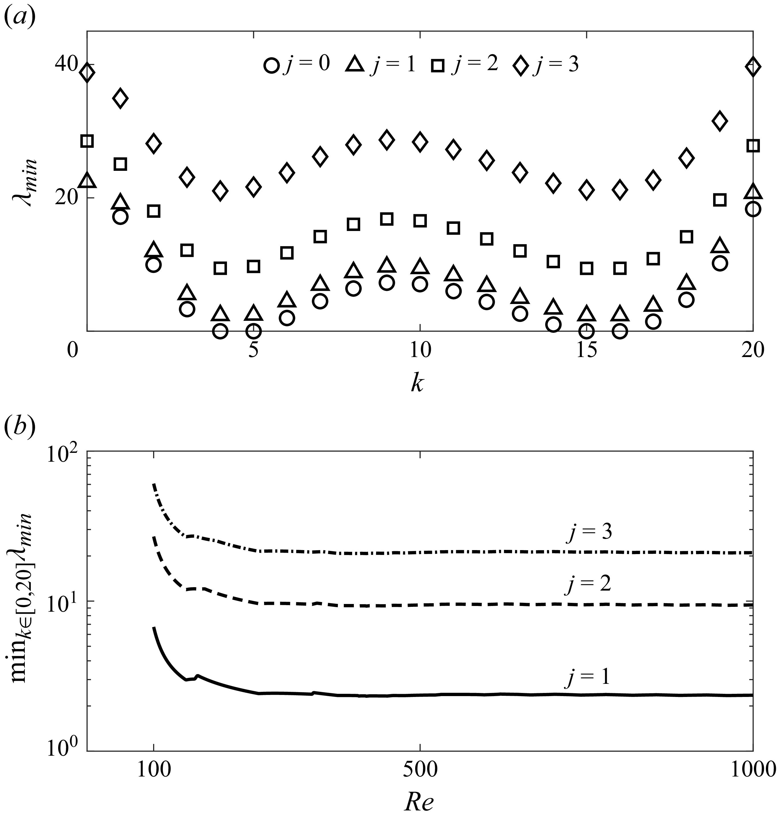


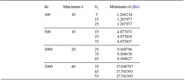


 Open access