


1. Introduction
In light of an increasing life expectancy and decreasing fertility, many countries have made adjustments to their pension systems. A typical reform in many countries was – and still is – raising the statutory retirement age (OECD, 2011). An obvious objective of this reform is that older individuals retire from the labor force at a later moment. A higher pension age has many other potential effects: it may impact household behavior (e.g. saving and consumption decisions), firm behavior (e.g. human capital investments, hiring, retaining, and firing decisions), and worker behavior (e.g. educational and health-related choices). The relevance of such effects is often not yet known. In this paper, we focus at the effect of the oldest partner’s statutory retirement age on both partners’ retirement choices and hours worked. This household perspective has not yet received much attention in the earlier literature.
We distinguish three channels that may play a role in the retirement decisions of households. First, financial incentives of the pension program(s) affect spousal labor force participation. Cross-effects between financial incentives for the one spouse on retirement behavior of the other are likely in case of joint optimization within the household (Van der Klaauw and Wolpin, Reference Van der Klaauw and Wolpin2008). Second, leisure complementarity could play a role in the retirement decision. In case the older spouse serves as the reference point for the younger partner for the preferred amount of leisure time, retirement of the oldest spouse could result in a larger taste for leisure for the younger partner as well. As a result, leisure complementarity implies that later retirement by one spouse will also lead to later retirement of the other spouse (Coile, Reference Coile2004; Schirle, Reference Schirle2008; Atalay et al., Reference Atalay, Barrett and Siminski2019). Third, social norms and reference points may affect retirement decisions around the statutory retirement age (Van Erp et al., Reference Van Erp, Vermeer and van Vuuren2014). Results found by Behaghel and Blau (Reference Behaghel and Blau2012) imply that retirement behavior in the US cannot be explained by just financial incentives, and that reference dependence and loss aversion may play a role. Results of Mastrobuoni (Reference Mastrobuoni2009) suggest that social norms play an important role in explaining retirement behavior. As mentioned by Seibold (Reference Seibold2021), several studies estimate the effect of pension reforms involving statutory retirement ages, but evidence on the direct effect of statutory ages is scarce. We contribute to this scarce literature, and as far as we know we are the first to investigate the direct effect of an increased statutory retirement age in the context of couples.Footnote 1 That is, we investigate the direct effect of spouse’s statutory retirement age on individual’s labor supply (in addition to their own statutory retirement age) and estimate these effects for successive cohorts with increasing statutory retirement ages. Furthermore, we investigate the effect of the old ‘traditional’ statutory retirement age of 65.
To estimate these effects, we use high-quality monthly Dutch administrative data, which are available for the whole Dutch population for the period January 2015–December 2018.Footnote 2 We exploit the discontinuity at the statutory retirement age and the stepwise increase in the statutory retirement age since 2013. In 2013, 2014, and 2015 the statutory retirement age increased by one month each year, and starting from 2016, it increased by 3 months per year. So, between 2015 and 2018, the statutory retirement age was raised by 6 months in total: from 65 years and 3 months to 65 years and 9 months. As a result of this gradual increase, cohorts face different statutory retirement ages.
Related to Deshpande et al. (Reference Deshpande, Fadlon and Gray2024), we use a regression discontinuity framework. Our double regression discontinuity design (Lalive and Parrotta, Reference Lalive and Parrotta2017) reveals how both spouses in a couple decide on their labor supply (in terms of hours worked and extensive margin) given the pension (in-)eligibility of their older partner. More precisely, we estimate the labor supply of the youngest partner as a function of their own and spousal age, their own and spousal statutory retirement age, and several control variables. Moreover, we run similar regressions to investigate hours worked (the intensive margin of labor supply).
In line with earlier findings, we find a direct effect of one’s own statutory retirement age of almost 30%. The oldest spouse’s statutory retirement age has a significant but small direct effect on the younger partner’s net labor force participation: almost 1%-point of females and 2%-points of males retire when their older spouse reaches the statutory retirement age. The results suggest that leisure complementarity plays a role, which is more affordable for high wage households than for low wage households. In addition, we find that the ‘traditional’ statutory retirement age still has an effect: when the older spouse already reached the retirement age, reaching the age of 65 by the younger female spouse increases retirement with 7%-points. For younger male spouses this effect is even 9.5%-points.Footnote 3
The contribution to the literature is threefold. We contribute to the literature of household decision making regarding the retirement decision. First, we identify how different spousal labor supply responses evolve when the statutory retirement age increases. In addition to earlier studies, we analyze labor supply responses for couples where the male partner is the younger partner (compare a.o. Zweimüller et al., Reference Zweimüller, Winter-Ebmer and Falkinger1996; Lalive and Parrotta, Reference Lalive and Parrotta2017). Also, we contribute to the literature on partial and phased retirement by investigating effects on the extensive and intensive margin (i.e. a measurement for the amount of hours worked). Finally, we add to the literature by zooming in on different income groups. We analyze whether household retirement behavior differs between high- and low-wage income groups.
The setup of the rest of this paper is as follows. Section 2 provides a literature review. Section 3 describes the institutional setting. Section 4 presents descriptive statistics and section 5 describes the estimation method and results. Section 6 shows a sensitivity analysis of our results. Lastly, section 7 provides a discussion of our findings and concludes.
2. Literature review
This section discusses the literature on household retirement. When considering household retirement decisions, the baseline models describe a problem of household coordination in which several channels play a role. In this review, we focus on three main channels, namely, financial incentives, leisure complementarity, and sociological and psychological channels. Thereafter, we discuss retirement research that has focused on the Netherlands.
2.1 Main channels in household retirement decisions
Starting with financial incentives, Blau and Gilleskie (Reference Blau and Gilleskie2006) and Van der Klaauw and Wolpin (Reference Van der Klaauw and Wolpin2008) build theoretical models in which the effect of retirement runs through the household budget constraint. Both papers explain how financial incentives of pension programs affect the labor participation decision of couples. Henretta and O’Rand (Reference Henretta and O’Rand1983) show that financial characteristics of both partners play a role in their retirement decisions. They find that the age of both partners’, their hourly wages, and pension entitlements affect the retirement decisions of each member in the household. In addition, Jousten and Lefebvre (Reference Jousten and Lefebvre2019) find that retirement considerations differ between men and women due to differences in earning position (first vs second earner).
The second channel concerns leisure complementarities. Hurd (Reference Hurd1990) studies joint retirement choices in models without uncertainty. Casanova (Reference Casanova2010) builds a model taking uncertainty into account when explaining how leisure complementarities affect the retirement decision of both household members. Michaud and Vermeulen (Reference Michaud and Vermeulen2011) build a model in which they model household utility as the weighted sum of male and female utility. Using this specification and making use of the Health and Retirement Study, their estimates show that leisure complementarity plays an important role in the retirement decision. Zweimüller et al. (Reference Zweimüller, Winter-Ebmer and Falkinger1996) draw a similar conclusion by examining how different statutory retirement ages for males and females in Austria affect spousal labor supply. They find that the female retirement age depends on the male’s retirement age but not vice versa. Lalive and Parrotta (Reference Lalive and Parrotta2017) confirm this finding by exploiting the difference in male and female statutory retirement ages in Switzerland. Garcia-Miralles and Leganza (Reference García-Miralles and Leganza2024) and Coile (Reference Coile2004) finds similar results when examining dual-earner couples in Denmark and the U.S, respectively. Schirle (Reference Schirle2008) shows that – due to the increase in retirement age in many G20 countries (see OECD (2011)) – the partner decided to work longer as well. Atalay et al. (Reference Atalay, Barrett and Siminski2019) discuss how an increase or decrease in the retirement age affects household labor supply decisions. Exploiting reforms in Austria and Vietnam, they find that the partner adjusts his or her labor supply regardless of whether there is an increase (Austria) or decrease (Vietnam) in the statutory retirement age. More specifically, the Vietnam veteran pension fund induced veteran’s wives to retire around 1.5–2.6 years earlier on average, while the estimates for Austria imply that a 5-year increase in female pension eligibility led husbands to retire later by 0.34–0.84 years on average.
Third, sociological and psychological effects may play a role in household retirement decision-making. Eismann et al. (Reference Eismann, Henkens and Kalmijn2019) discuss two possible channels of how the individual can influence the partner’s labor supply decision. First, there is the channel of altruism. This channel states that, since retirement is generally associated with healthier behavior (Syse, Reference Syse2017), an individual that cares about the partner’s health might want that the partner to retire. Second, there is the channel of self-interest. Individuals want their partner to retire early if it benefits him or herself. This is for instance the case when the quality of the relationship is high or when long working days of the other person negatively affects the well-being of the other person. Another channel focuses on the importance of mental health. Picchio and Van Ours (Reference Picchio and Van Ours2019) find that mental health differs between males and females after retirement. Single men tend to experience a drop in mental health. For males with a partner, the effect is positive: they experience a positive effect on their mental health as well as their partner’s mental health. On the other hand, female retirement hardly has any effect on their own mental health or the mental health of the partner. Moving away from sociological channels within the household, the initial age at which older workers were eligible for pension benefits may as well play a role in the retirement decision. More precisely, Behaghel and Blau (Reference Behaghel and Blau2012) argue that the initial age of 65 at which social security payments became available is still an important reference point for workers that are eligible at a higher age. The authors argue that a combination of the initial reference point combined with loss aversion of leisure due to an increase of the statutory retirement age may make workers less likely to work longer and instead retire at the age of 65. In a similar vein, Seibold (Reference Seibold2021) shows that statutory retirement ages in Germany are an effective policy tool to influence retirement behavior. This is not the case for the US where an increase in the retirement age does not seem to result in an increase in labor supply (Deshpande et al., Reference Deshpande, Fadlon and Gray2024).
2.2 Retirement research in the Netherlands
Having discussed the most important channels affecting joint retirement decisions, it is important to discuss what research regarding these channels has already been conducted for the Dutch pension system. Considering financial incentives, Atav, Jongen, and Rabaté (Reference Atav, Jongen and Rabaté2019) and Koning et al. (Reference Koning, Gelderblom, Gravesteijn and de Vleeschouwer2017) show that the gradual increase in the statutory retirement age as of 2013 increased the individual labor supply of older Dutch workers.
Focusing on spousal retirement, Deelen and van Vuuren (Reference Deelen and van Vuuren2009) argue that an increase in the education levels resulted in a higher employment rate for both males and females, resulting in a higher earning capacity for both (i.e. higher opportunity costs for not working). Moreover, an increase in the female education level increased the likelihood of being employed at later ages, making it for the partner less attractive to retire early. The reason for this is that males/females postpone their (early) retirement decision due to leisure complementarity. Analyzing the female labor force participation, Euwals et al. (Reference Euwals, Knoef and van Vuuren2011) argue that social norms influence the decision to participate and conclude that cohort effects are important for females born between 1935 and 1955. They postulate that the role of social norms and attitudes towards paid employment is important in explaining the development of female labor force participation over successive cohorts. Hospido and Zamarro (Reference Hospido and Zamarro2014) make use of SHARE data to investigate joint retirement decisions in several European countries including the Netherlands. Exploiting the early retirement and official retirement possibilities in those countries, they find a joint retirement effect for women, but not for males. García and van Soest (Reference García and van Soest2022) discuss how the abolition of partner pension in the Netherlands changes the joint retirement decision. They point to a change in financial incentives as well as a change in the social norm that decreases the likelihood of retiring together. Lastly, Bloemen et al. (Reference Bloemen, Hochguertel and Zweerink2019) discuss how early retirement incentives affect retirement behavior of the partner. To do so, they exploit an attractive early retirement policy for civil servants. They find that early retirement incentives for male civil servants induced their wives’ probability to retire by 10 percentage points. On a larger scale, Oral et al. (Reference Oral, Rabaté and Seibold2024) analyze how the abolishment of a financially attractive early retirement scheme affects retirement behavior. They find strong spillover effect for partners of up to 9 months increase in employment duration.
3. Institutional setting
We describe the institutional setting in the Netherlands. We first discuss the Dutch pension system and thereafter we discuss other relevant programs that could be used as pathways into early retirement.
3.1 Dutch pension system: set-up
Like most modern pension systems, the Dutch pension system consists of three pillars, which allow workers to accumulate pension rights approximately equal to 70% of their average gross wage over their working life. The first pillar is the pay-as-you-go publicly funded pension benefits (in Dutch: AOW). Individuals start receiving these benefits from the statutory retirement age. Each individual that has lived for 50 years or more in the Netherlands receives an amount equal to 70% (50%) of the minimum income after reaching the statutory retirement ageFootnote 4 when he or she lives alone (with a partner).Footnote 5 A policy review of the Ministry of Social Affairs shows that the take-up rate of public pension benefits is high and that it successfully eliminates poverty among older individuals.Footnote 6
The second pillar pension is the pension that the employer and employee jointly save via a pension fund or insurance company. Unlike the first pillar, this pension pillar heavily depends upon work history and earnings per year. Another difference is that it is possible to withdraw second pillar pension benefits before the (first pillar) statutory retirement age. Lastly, the third pillar consists of own individual savings on top of the first and second pillars. Under some conditions it is possible to make tax-favored pension savings within this pillar.
3.2 Reforms in the first pillar of the Dutch pension system
The Dutch first pillar pension scheme faced two major reforms in the past decade.Footnote 7 First, the first pillar partner pension was abolished. Before January 1st, 2015, individuals received partner pension from the statutory retirement age if their partner did not yet reach this age. The amount of first pillar partner pension depended on the partner’s income (Van den Berg et al., Reference Van den Berg, Klabbers, de Pijper, Sens, Wildenburg and Hop2007). First pillar partner pension was abolished to keep the pension system sustainable. Moreover, it was deemed less necessary since the increase in the economic independence of female partners.
The second major reform is the gradual increase of the statutory retirement age. Up to January 1st, 2013, the first pillar statutory retirement age was 65 years. In 2013, 2014, and 2015, the statutory retirement age increased by one month each year. In 2016, 2017, and 2018, the statutory retirement age increased by three months per year. Table 1 provides a precise overview of the statutory retirement age per year and birth cohort.
Table 1. The statutory retirement age for different birth cohorts. it is not possible to withdraw first pillar pension benefits prior reaching the statutory retirement age
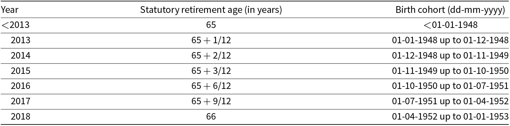
Source: rijksoverheid (Reference Rijksoverheid2019)
3.3 Reforms in the second pillar of the Dutch pension system
Workers can take up the second pillar pension before reaching the first-pillar statutory retirement age. However, the Dutch government made it less attractive to retire at an earlier age. For instance, pre-retirement pension arrangements between employers and employees were heavily restricted after 2006. Until 2006, the Dutch government subsidized early retirement routes. In 2006, this became gradually more restricted and a Life Cycle Saving Footnote Scheme 8 was introduced. This arrangement was introduced to compensate individuals that reached the retirement age before January 1st, 2015. Although this arrangement was less attractive than the earlier arrangements, it was still financially attractive for younger partners to exit the labor force at a younger age, making it easier for couples to coordinate their joint retirement decision (for instance when one partner reaches the statutory retirement age). Moreover, this implies that cohorts after 2015 are not comparable to cohorts before 2015 as younger partners can no longer make use of this scheme (Van den Berg et al. Reference Van den Berg, Klabbers, de Pijper, Sens, Wildenburg and Hop2007).
3.4 Pathways into early retirement and legal changes
The increase of the statutory retirement age and the abolition of early retirement programs and lifecycle saving schemes may cause substitution towards other social security programs. Over the last two decades, successive Dutch administrations tried to prevent this form of social support substitution.Footnote 9 At the beginning of the 21st century, the government reduced the attractiveness of disability insurance. As of 2002, they came up with stricter reintegration rules in case of sickness. In 2003, sickness benefit became less generous for workers employed by small firms and in 2008 it was implemented for all firms.
The maximum duration of unemployment insurance has been gradually decreased. From 2003 onwards, it is no longer possible to receive unemployment benefits up to retirement starting at the age of 57.5.Footnote 10 In 2006, the maximum benefit duration decreased from five years to three years and two months. As of 2015, the generosity of unemployment insurance was further reduced. Between January 1st, 2016, and January 1st, 2018, the benefit duration decreased gradually from 38 towards 30 months. Moreover, it takes more working years to get the full amount of benefit duration (de Pijper et al., Reference de Pijper, Wildenburg, Montessori, van de Graaf, de Jong, Van der Zanden and Ramaekers2019).Footnote 11 However, this reform mostly affects workers with a large labor market history and therefore a large second pillar pensions benefit.Footnote 12 Nevertheless, all these measures seem to have limited alternative early retirement pathways via other social security programs (Ministry of Social Affairs, 2019).
Lastly, it is as important to analyze the conditions which allows workers to continue working beyond the statutory retirement age. Most sectors of industry can dismiss workers without any costs as soon as they reach the statutory retirement age.Footnote 13 As a consequence, workers in these sectors cannot continue in the job they had after reaching the statutory retirement age. A legal change in the Netherlands in the period 2014–2018 is the ‘Continuing to work Act’Footnote 14, which makes it more attractive for employers to retain workers after they reached the statutory retirement age. For instance, the notice period for dismissal for this group is reduced to one monthFootnote 15 and the obligation to continue wage payment in case of illness is reduced to six weeks (instead of two years).
4. Descriptive statistics
We use administrative microdata from Statistics Netherlands (Statistics Netherlands (CBS), s.d.) to analyze the effect of pension eligibility on spousal labor supply. This rich administrative datasetFootnote 16 allows us to trace individuals on a monthly basis. From this dataset, we select heterosexual couples that are married or have a registered partnership and stay together over the period 2014–2018.Footnote 17 We limit ourselves to households in which household members are not in the same pension cohort (Table 1) and the oldest spouse reaches the public statutory retirement age from 2015 onwards.Footnote 18 Moreover, we only include couples in which the oldest partner works as an employee or is retired (i.e. the oldest spouse is excluded in case he is self-employed).Footnote 19 We also exclude couples in which the youngest partner is self-employed.Footnote 20 This leaves us with approximately 20,000 (2,500) observations for three different pension cohorts in which the male (female) is the oldest spouse.
For these couples, we have data on their monthly earnings, ethnicity (first, or second generation immigrant), and whether at least one child is living within the household. Table 2 provides summary statistics for these households for couples in which the male (columns 1–3) and female (columns 4–6) is the oldest spouse.
Table 2. Summary statistics male (old), female (young) and female (old), male (young) by public pension eligibility of the oldest spouse. The shaded areas indicate the year after the oldest spouse reaches the pension eligibility age. The part-time factor is a standardized measurement of the number of hours worked, where one indicates that individuals work full-time and zero indicates no hours worked. The mean labor income is reported for individuals who have labor income larger than zero
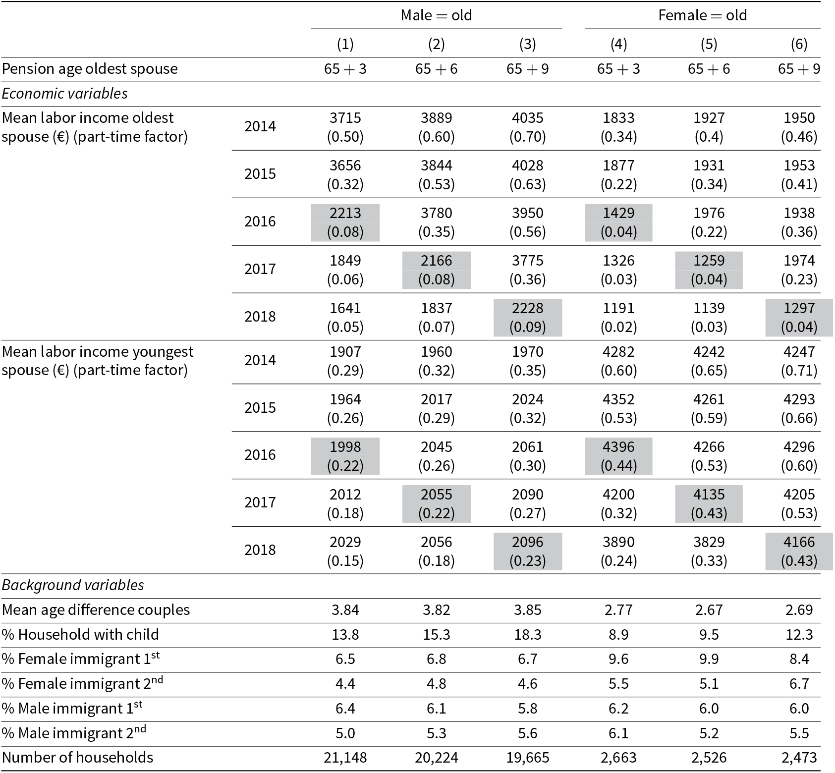
The upper part of Table 2 shows the mean monthly labor income per year of the oldest and youngest spouse provided that the income is larger than zero. We observe that average male income is in most cells higher when compared to average female income. Moreover, we observe a strong decline in the average income of the oldest spouse in the years after retirement (the shaded area). The younger partners do not face a similar decrease in income.
In brackets below the monthly mean annual labor income, we report the mean annual part-time factor. The part-time factor is defined as hours worked divided by full-time hours. For instance, if an individual worked 15 full-timeFootnote 21 days (roughly 78 hours) and a full-time job in a particular month consists of 30 days (roughly 156 hours), the part-time factor for this person is equal to 0.5. In case an individual did not work in a particular month, we set the part-time factor equal to zero. The biggest drop in the part-time factor for the oldest spouse is observed one year after (the majority of) a particular cohort reaches the retirement age. For younger partners, who observe a smaller reduction. This difference is largest for couples where the female is the oldest spouse.
Table 2 provides also on information on several background variables (age difference, ethnicity, and the percentage of households with children). The age difference between the spouses equals approximately 3.8 years (2.8 years) for couples where the male (female) is the oldest spouse. The percentage of households with children fluctuates between 8.9% and 18.3%, where the presence of children is more frequent for couples where the male is the oldest spouse. Having children that still live at home (and the corresponding costs associated with it) may have the intention to retire relatively late when compared to couples where this is not the case.Footnote 22
In addition, the share of first-generation female immigrants is approximately 6.5% and 10%, where the percentage is higher for couples where the female is the oldest spouse. A similar pattern is visible for second generation female immigrants. The share of first and second generation male immigrants is between 5% and 6.2% across all cohorts. It is important to take this into account as first-generation immigrants may not be entitled to the full first pillar pension benefits.Footnote 23
4.1 Graphical evidence
We plot the average net labor force participation (percentage of the employed spouses) of the youngest spouse 6 months prior and after the older spouse reaches the statutory retirement age for all couples that are not in the same pension cohort. We do this for both types of couples where respectively males and females are the oldest spouse.
The graphs below visualize how the younger partner reacts to the statutory retirement age of their older spouse. Analyzing Figure 1, we observe a small discontinuity in the labor supply of the younger partner when the older male spouse reaches his pension eligibility age. The drop in average labor force participation of the younger spouse one month prior and one month after the oldest spouse reaches his statutory retirement age is approximately 0.5 to 1 percentage points. In Figure 2, we provide graphical evidence for couples where the female is the oldest spouse. We observe here a similar pattern as in Figure 1, although the decrease in average labor force participation is somewhat larger for the younger male partners.
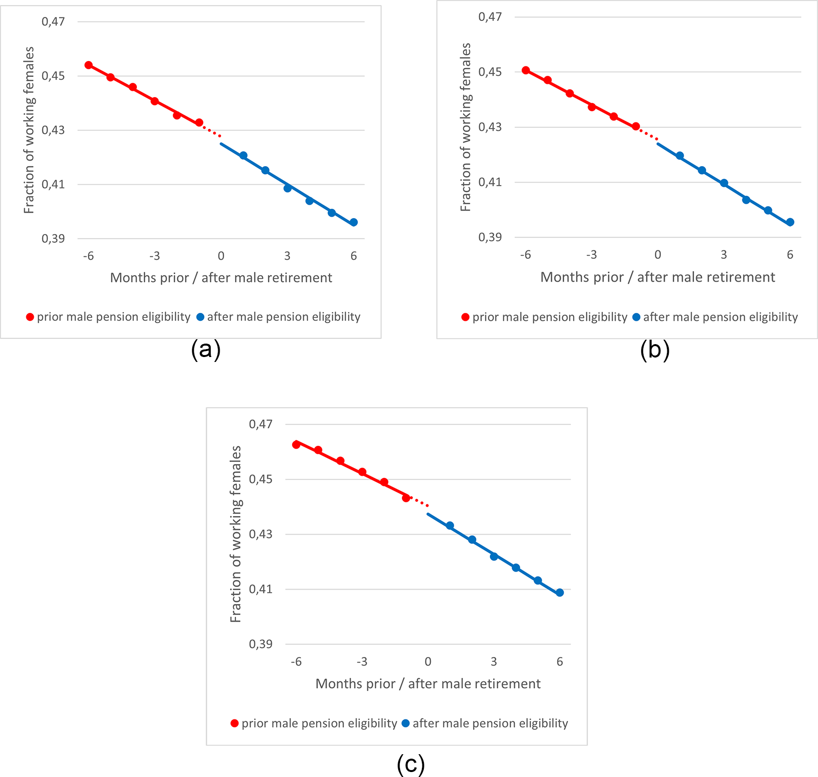
Figure 1. The effect of male pension eligibility on the net labor supply of the younger female partner. Figure (a) for older male partners with a pension eligibility age of 65 years and 3 months, figure (b) for older male partners with a pension with a pension eligibility age of 65 years and 6 months, and figure (c) for older male partner with a pension eligibility age of 65 years and 9 months. The red (blue) line indicates the net labor force participation of the younger partner 6 months prior (after) retirement of the older spouse.
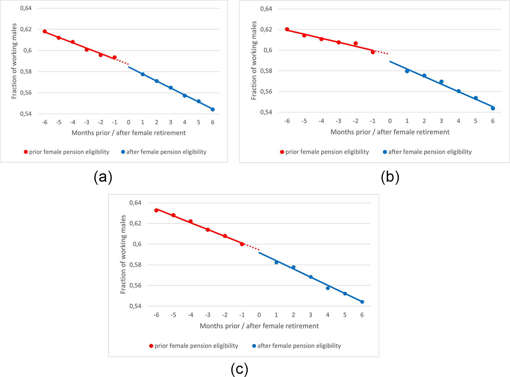
Figure 2. The effect of male pension eligibility on the net labor supply of the younger female partner. Figure (a) for older male partners with a pension eligibility age of 65 years and 3 months, figure (b) for older male partners with a pension with a pension eligibility age of 65 years and 6 months, and figure (b) for older male partner with a pension eligibility age of 65 years and 9 months. The red (blue) line indicates the net labor force participation of the younger partner 6 months prior (after) retirement of the older spouse.
Appendix A.1 shows graphs that visualize how males and females react to their own pension eligibility. These graphs show a strong decline in labor force participation at the moment someone is entitled to first pillar pension benefits, indicating that individuals react strongly to their own pension eligibility.
5. Estimation method & results
We estimate the effect of an increase in the Dutch statutory retirement age on the partner’s net labor force participation by using a double regression discontinuity designFootnote 24 (D-RDD) as is advocated by Lalive and Parrotta (Reference Lalive and Parrotta2017). Exploiting the fact that different pension cohorts have a different statutory retirement age, we can also determine whether spousal’s net labor force participation changes with the increased statutory retirement age of the older partner. We as well use this regression output to explain whether leisure complementarity between partners increases or decreases. Thereafter, we analyze the part-time factor, which measures the labor-supply of the youngest partner at both the intensive and extensive margin. Lastly, we analyze whether social norms play a role. We do this by analyzing how the initial retirement age of 65 affects the net labor force participation.
5.1 Labor supply of the youngest spouse
We estimate the effect of reaching the statutory retirement age on the net labor force participation of the youngest partner. To do so, we estimate a linear probability model:
 \begin{equation}\begin{array}{l}{Q_y} = \alpha + {\beta _1}{R^y} + {\beta _2}{R^o} + {\beta _3}\left( {Ag{e^y} - Age\left( {{R^y}} \right)} \right) + {\beta _4}\left( {Ag{e^o} - Age\left( {{R^o}} \right)} \right) \\ \quad\quad +\,\,{\beta _6}\left( {Ag{e^y} - Age\left( {{R^y}} \right)} \right)*{R^y} + {\text{ }}{\beta _6}\left( {Ag{e^o} - Age\left( {{R^o}} \right)} \right)*{R^o} + {\beta _7}X + \varepsilon \end{array}\end{equation}
 The above regression measures how the net labor force participation of the youngest partner in the current month depends on the statutory retirement age of the older partner and his or her own pension eligibility. More precisely,  ${Q_y}$ denotes the labor supply of the youngest partner $y$, which is equal to unity if the partner worksFootnote 25 and is equal to zero otherwise. $\alpha $ denotes a constant. ${R^o}{\text{ }}$ and ${R^y}$ are dummy variables that indicate whether the oldest (o) and youngest (y) partner are eligible for public pension benefits in a particular month. If this is the case, the dummy is equal to unity. The terms $Ag{e^o} - Age\left( {{R^o}} \right)$ and $Ag{e^y} - Age\left( {{R^y}} \right){\text{ }}$ denote the difference in months between the age of the oldest and younger partner’s age and their corresponding statutory retirement age. $Ag{e^o}$ and $Ag{e^y}$ are increasing each month as each person’s age increases over time. ${\beta _5}$ and ${\beta _6}$ measure the interaction between the pension eligibility dummy and the difference between the current age and the statutory retirement age. We include these interaction terms to allow for a different trend in labor participation before and after the statutory retirement age. Lastly, $X$ denotes several control variables for the household members and $\varepsilon $ denotes the error term. $X$ includes variables that indicate whether one of the individuals is a first- or second-generation immigrant and whether any children are living in the household. Lastly, we include a set of year dummies and (pension) cohort dummiesFootnote 26 for the younger partner as control variables. We run the above regression separately for each pension cohort of the older spouse. By analyzing the effect of spousal labor supply for individuals with different statutory retirement ages we can see whether spousal labor supply reacts stronger or weaker when the oldest partner has a higher statutory retirement age.
The main coefficient of interest is  ${\beta _2}$. This coefficient captures how the youngest partner reacts to the statutory retirement age of the older partner. A negative sign indicates a reduction in the net labor force participation of the younger partner when the oldest spouse reaches the statutory retirement age. A positive sign would indicate an increase in the net labor force participation. Table 3 shows the ${\beta _1}$ and ${\beta _2}$ coefficients for the case where the male is the oldest partner and the female is the oldest partner, respectively. The full regression output of regression (1) is displayed in Appendix B.1.
Table 3. The effect of pension eligibility of the older spouse on the net labor supply of the younger partner. The regression formula is given by equation (1) and the corresponding coefficients are presented in the uneven columns. We control for first- and second-generation immigrant status, the presence of children in the household, cohort dummies, and year effects. The even column present the percentage change in net labor force participation, which is the quotient of the regression coefficients in the even columns and the average net labor force participation at the moment of pension eligibility of the oldest spouse. Clustered standard errors at the household level are between parentheses
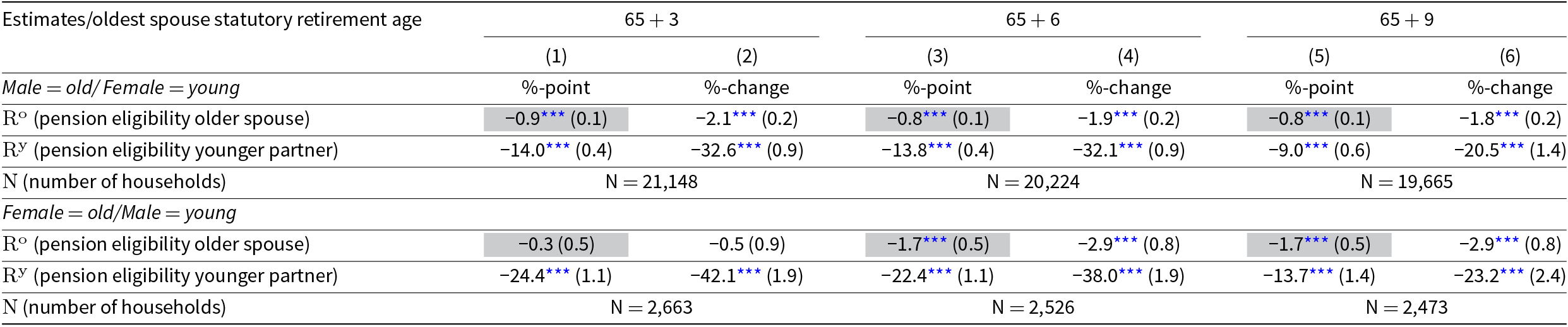
*** denotes significance at 1%. See Appendix B.1 for the full regression output.
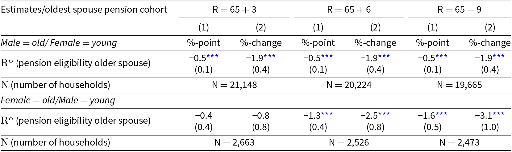
Table 3 shows the effect of pension eligibility of the oldest partner on the net labor force participation of the younger spouse (Table 3:  ${R^o}$ rows, uneven columns). Focusing on couples where the male is the oldest spouse, we find that the effect of male public pension eligibility decreases female’s net labor force participation by approximately 0.8 percentage points. When analyzing couples where the female is the oldest spouse, the estimates are in a range of minus 0.3 percentage points to minus 1.7 percentage points, although the estimate is insignificant for the cohort with statutory retirement age of 65 + 3. Overall, the above results indicate consistently negative and significant effect across pension cohorts regardless of the gender of the oldest spouse.
In addition, we calculate the percentage change in net labor force participation for the younger partner when the oldest spouse reaches the statutory retirement ageFootnote 27 (Table 3:  ${R^o}$ rows, even columns). For couples where the male is the oldest partner, we find that this percentage change is around 2 percent for all statutory retirement ages. For couples where the female is the oldest spouse, the effect is approximately equal to minus 0.5 (insignificant) and minus 2.9 percent for the last two cohorts (65 + 6 and 65 + 9).
Lastly, the results show that younger spouses react stronger to their own pension eligibility than to the pension eligibility of the older partner (Table 3:  ${R^y}$ rows). Overall, this effect is negative and significant at the 1 percent level and ranges from minus 9.0 (13.7) percentage points to 14.0 (24.4) percentage points for couples where the male (female) is the oldest spouse. Analyzing the percentage change in net labor force participation, we find that the own pension eligibility decreases labor supply by 20 to approximately 33 percent for couples where the male is the oldest spouse. For couples where the female is the oldest spouse, the effect ranges from minus 23.2 to minus 42.1 percent.
5.2 Income effect and leisure complementarity
We analyze whether the retirement behavior of couples differs for different pension cohorts. Therefore we first determine how the pension eligibility age of the oldest spouse affects their own net labor supply. To do so, we slightly change regression equation (1) by choosing the net labor force participation of the older spouse ${\text{ }}({Q_o}){\text{ }}$as our dependent variable.Footnote 28 The main coefficient of this regression is (as well) ${\beta _2}$ as it indicates how the older partner changes his or her net labor supply at the extensive margin after reaching his or her own statutory retirement age. The main results of this regression are summarized in Table 4.Footnote 29
Table 4. The effect of pension eligibility of the older spouse on his/her own net labor supply. the regression formula is given by equation (1) with the net labor supply of the older spouse as dependent variable. We control for first- and second-generation immigrant status, the presence of children in the household, cohort dummies, and year effects. Clustered standard errors at the household level are between parentheses
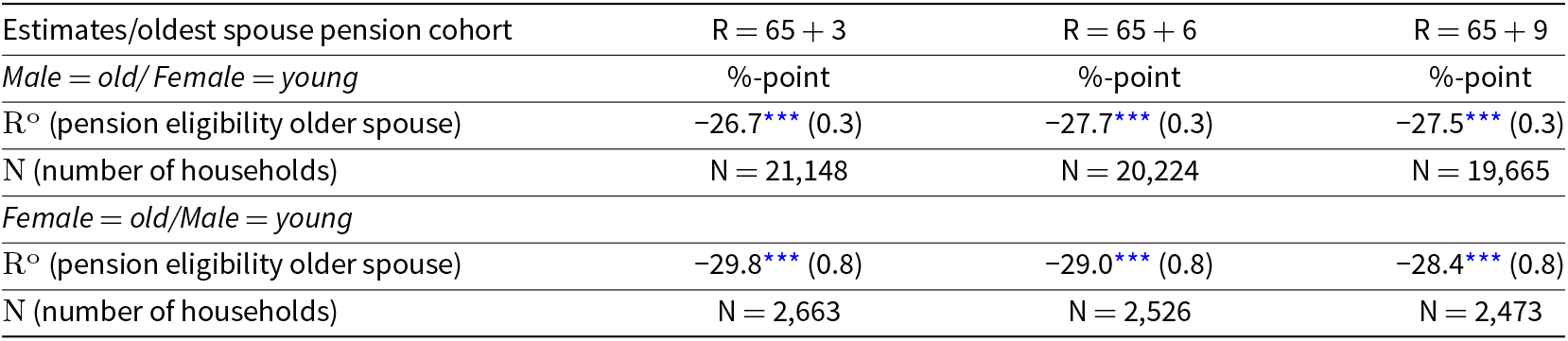
*** denotes significance at 1%. See Appendix B.2 for the full regression output.
We observe that the coefficients range from minus 26.7 to minus 27.7 (minus 28.4 to minus 29.8) for couples where the male (female) is the oldest spouse. These effects are relatively constant for all pension cohorts.Footnote 30 Using these findings, we calculate the ratios between the estimated coefficients in Table 4 and the shaded coefficients in Table 3. These ratios indicate how sensitive the younger spouse’s net labor force participation is with respect to the net labor force participation of the oldest spouse. Table 5 presents these ratios.
Table 5. The ratio of the net labor force participation of the younger partner with respect to the net labor force participation of the older spouse. More formally, we calculate ( $(d{Q^y}/d{R^o})/(d{Q^o}/d{R^o})$. To obtain the numerator (denominator) of this fraction, we regress equation (1) on the net labor supply of the younger (older) spouse. These regression results are presented in appendix B.2. Standard errors clustered at the household level are between parentheses
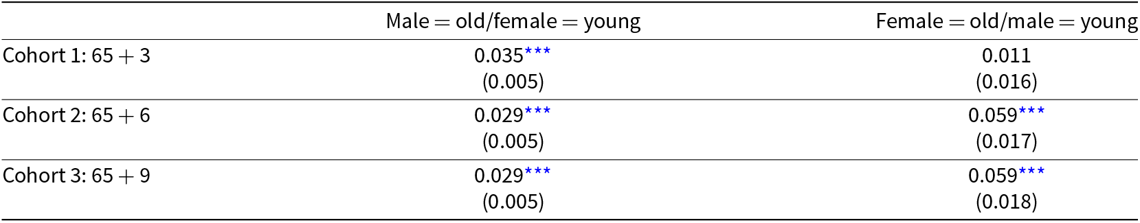
* denotes significance level at 10%, **denotes significance at 5%, and ***denotes significance at the 1% level.
The results show that around 3% of younger female partners stops working (extensive margin) when the older male spouse stops working at the statutory retirement age. This is similar across all three different pension cohorts. For couples where the female is the oldest spouse, we observe that this ratio is approximately 6%. The exception is the oldest cohort, for which we only find an effect of 1% (not significantly different from zero).
Finally, we divide each pension eligibility cohort into a low wage and high wage income household based on the total household wage income in January 2014. Thereafter we run the regression (1) on these subgroups and calculate the above-mentioned ratio for low- and high wage income households.Footnote 31 The ratios for the different wage income groups per pension cohort are provided in Table 6. We find that these ratios are about twice as large for the high wage income group compared to the low wage income group. This pattern might be explained by leisure complementarity as this is more affordable for high wage households than for low wage households.
Table 6. The ratio of the net labor force participation of the younger partner with respect to the net labor force participation of the older spouse for different wage income groups. More formally, we calculate  $(d{Q^y}/d{R^o})/(d{Q^o}/d{R^o})$. To obtain the numerator (denominator) of this fraction, we regress equation (1) on the net labor supply of the younger (older) spouse for different income groups. These regression results are presented in appendix B.3. Standard errors clustered at the household level are between parentheses
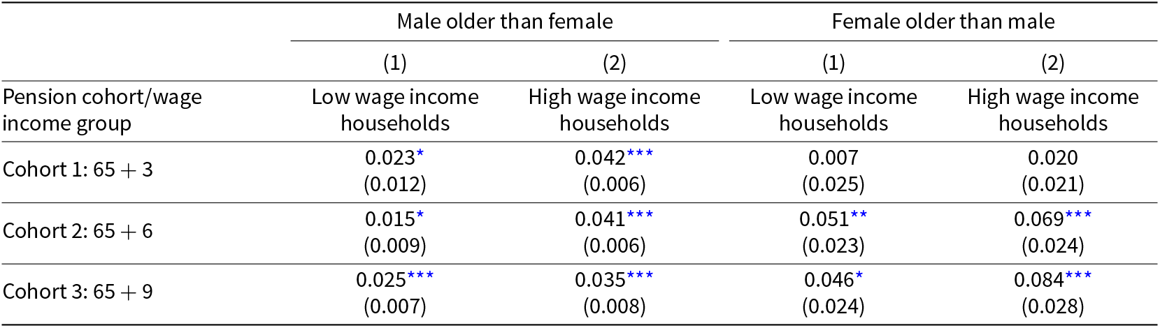
* denotes significance level at 10%, **denotes significance at 5%, and ***denotes significance at the 1% level.
5.3 Part time factor
We use the part-time factor to analyze how the pension eligibility age of the oldest spouse affects labor supply of the younger partner at the intensive and extensive margin (i.e. number of full-time days worked). In Appendix A.2, we present graphs showing how the part-time factor of the younger partner changes before and after the older partner receives pension benefits. They provide a similar image as the graphs in section 4. The regression we run is equal to regression (1), only changing our dependent variable to the part-time factor of the younger spouse (including zeros).
Table 7 shows the percentage point change and the percentage change in the part-time factor of the younger partner after pension eligibility of the older spouse.Footnote 32 For couples where the male is the oldest spouse, the part-time factor of the younger partner reduces by approximately 0.5%-points when the male becomes eligible for pension benefits. The results are similar for couples where the female is the oldest spouse, except that that the estimate for couples with a statutory retirement age of 65 + 3 is not significant at the 5% level. Comparing Table 7 with Table 3, we find that the relative changes on the extensive and intensive margin as well as the percentage changeFootnote 33 follow approximately a similar pattern.
Table 7. The effect of pension eligibility on the part-time factor of the younger spouse. We control for first- and second-generation immigrant status, the presence of children in the household, cohort dummies, and year effects. Clustered standard errors at the household level are between parentheses
*** denotes significance at 1%. The full regression output is available in Appendix B.4.
5.4 Social norms
Since the introduction of the first pillar pension benefits in the Netherlands in 1956, the statutory retirement age was set at the age of 65. Up to 2013, this statutory retirement age never changed. Therefore this initial retirement age could still play a role as reference point and may affect the labor force participation decision of the older partner (Behaghel and Blau, Reference Behaghel and Blau2012).
We analyze whether the age of 65 serves as an important referent point for the younger partner by running the following regression:
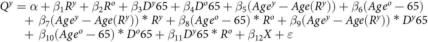 \begin{equation}\begin{array}{l}{Q^y} = \alpha + {\beta _1}{R^y} + {\beta _2}{R^o} + {\beta _3}{D^y}65 + {\beta _4}{D^o}65 + {\beta _5}(Ag{e^y} - Age({R^y})) + {\beta _6}(Ag{e^o} - 65) \\ \quad\quad +\,\,{\beta _7}(Ag{e^y} - Age({R^y}))*{R^y} + {\beta _8}(Ag{e^o} - 65)*{R^o} + {\beta _9}(Ag{e^y} - Age({R^y}))*{D^y}65 \\ \quad\quad +\,\,{\beta _{10}}(Ag{e^o} - 65)*{D^o}65 + {\beta _{11}}{D^y}65*{R^o} + {\beta _{12}}X + \varepsilon \end{array}\end{equation}
 In the above regression, most of the variables have the same interpretation as in regression (1). However, we changed ( $Ag{e^o} - Age\left( {{R^o}} \right)$) to $\left( {Ag{e^o} - 65} \right)$ as now the age of 65 is the main age of interest.Footnote 34 Besides, we added two dummy variables ${D^y}65$ (and ${D^o}65$) which are equal to unity when the younger partner (older partner) reaches the age of 65. If this is not the case, the variable equals zero. We as well add interaction terms between the age difference and the ${D^y}65$ and ${D^o}65$ variables. Lastly, we add the interaction term between the two dummy variables ${D^y}65$ and ${R^o}$. This interaction term indicates whether the younger partner retires at the age of 65 when the older spouse is eligible for first pillar pension benefits. Given that the age of 65 still serves as a reference point, this is our main coefficient of interest as it indicates whether the reference point plays a role when the older partner is already eligible for first pillar pension benefits. Table 8 provides an overview of the main coefficients of interests.Footnote 35
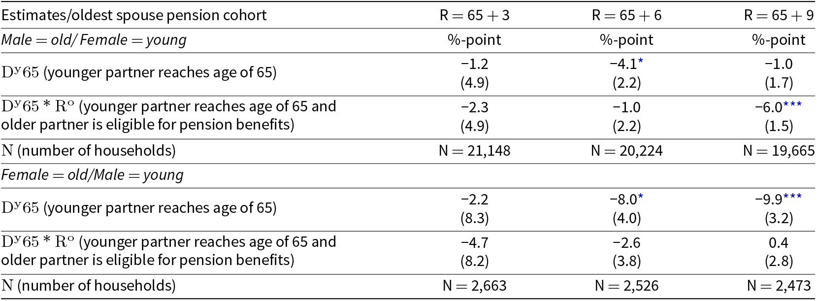
Table 8. The effect of reaching the age of 65 by the younger partner on their labor supply. We control for first- and second-generation immigrant status, the presence of children in the household, cohort dummies, and year effects. Clustered standard errors at the household level are between parentheses
* denotes significance level at 10% and *** denotes significance at 1%. The full regression output is available in Appendix B.5.
We observe that the net labor force participation of the younger partner decreases once the younger partner reaches the age of 65. This effect is not significantly different from zero for the oldest cohort with a statutory retirement age of 65 + 3. For the youngest cohort the effect is the largest when the older partner reached the statutory retirement age. So, there is a social norm effect for the ‘old’ statutory retirement age for the youngest partner, especially when the older partner already reached the (new) statutory retirement age. Since financial incentives are not likely to play a role at age 65 for the younger partner (e.g. no access to pension benefits), the main mechanisms that could explain retirement behavior of the younger partner at this age are social norms and/or leisure complementarity.
6. Sensitivity analysis
To check for robustness of our results, we relax some of the assumptions we made so far. First, we allow the oldest spouse to have self-employed as their main source of income.Footnote 36 Although we do not observe their labor supply at a monthly level, we can still see whether their younger partner reacts once they are eligible for pension benefits (both in terms of net labor supply and part-time factor). The results are displayed in Appendix B.6. We find that our results do not change in terms of sign or significance, regardless of cohort and gender of the oldest spouse.
In addition to the above relaxation, we also change the month in which the net labor force participation of the younger partner may change. A reduction in net labor force participation of the younger partner in the month when the older spouse reaches the pension eligibility age might be too restrictive. Therefore, we analyze in Appendix B.6 the effect on the net labor force participation of the younger spouse when using the net labor supply at time  $t + 1,{\text{ }}t + 2,$ and ${\text{ }}t + 3$ as dependent variable. We find that the coefficients remain relatively constant, indicating that the main reduction in net labor supply of the younger partner happens when the oldest spouse reaches the pension eligibility age.
7. Discussion & conclusion
We analyzed how spousal labor supply is affected by the statutory retirement age of the oldest spouse. The regression results also show a negative effect on the net labor participation of the younger spouse. Younger partners decrease their labor supply at the extensive margin up to 1.7 percentage points once the oldest spouse reaches the statutory retirement age. The responsiveness for younger men is twice as high than for younger female partners. The responsiveness is also about twice as strong in high-wage income households than in low-wage income households. The responsiveness in terms of hours worked are somewhat smaller. Lastly, we show evidence that for younger spouses the original statutory retirement age of 65 is still a reference point. This indicates that, in addition to the leisure complementarity, social norms also seem to impact retirement decisions.
In general, the negative participation effect we find can be caused by leisure complementarity, financial incentives and/or social norms. The ratio, which shows how sensitive the younger spouse’s net labor force participation is with respect to the net labor force participation of the oldest spouse, is constant for different pension cohorts of the older spouse. The same holds as well when we investigate this ratio for different wage income groups. Therefore, leisure complementarity likely plays a role in the decision-making process.
On the other hand, we as well observe that these ratios are almost twice as high for couples where the male is the younger spouse. This might be explained by a smaller age difference for these couples. A smaller age difference means that the own statutory retirement age of both spouses are relatively close to each other. As a result, retiring prior to the own pension eligibility age has a less negative impact on lifetime income. Reducing the number of working hours today does not only affect current income, but also second pillar retirement income. If the younger partner is closer to the own retirement age, the reduction in the second pillar pension income will be limited. The importance of this mechanism is a question for future research.
In addition, the complementarity ratios are also 1.5 to 2 times higher for high wage income households. Therefore, it seems that the richer the household, the more likely both partners will retire together. The first pillar pension benefits the older partner receives when retiring equals fifty percent of the minimum wage. This is most likely inadequate financial compensation to withdraw from the labor force for the younger partner unless there is sufficient second pillar pension available such that the younger partner can retire as well. High wage households often have mandatory and high second pillar pensions and are therefore more likely to retire jointly. This suggests that leisure complementarity plays a larger role than liquidity constraints (i.e., access to public pension benefits) since high wage income households are less dependent on public pension benefits. The analysis on the initial retirement age of 65 also points in that direction.
Supplementary material
The supplementary material for this article can be found at https://doi.org/10.1017/S1474747225000046.
Acknowledgements
We would like to thank all participants at the Netspar Theme conference on work, health, and retirement, Netspar Pension Day, KvS New Paper Sessions, the Dutch Economist’ Day, the TiU ZJU PhD workshop, a seminar at Tilburg University, and ESPE conference for their contributions. All remaining errors are our own.
This paper uses confidential micro data from Statistics Netherlands (CBS). The datasets we use can be obtained by filing a request directly to CBS. The above-mentioned authors are willing to help others to get access to these datasets.
Funding statement
This research was funded by Institute Gak. Institute Gak contributes to the quality of social security and the labor market in the Netherlands by investing in social projects and academic research.


