


1. Introduction
Turbulent dispersion is relevant for understanding many natural and engineered flows, e.g. the spreading of plankton in aquatic ecosystems, the transmission of hazardous aerosols in the atmosphere, and the mixing of components in process engineering, to name a few (Toschi & Bodenschatz Reference Toschi and Bodenschatz2009; Bourgoin & Xu Reference Bourgoin and Xu2014; Brandt & Coletti Reference Brandt and Coletti2022; Huang et al. Reference Huang, Liu, Song, Yin and Wang2025). When the particles cannot be approximated as tracers, their inertia and the buoyancy forces to which they are subject greatly complicate the dispersion under the influence of the turbulence. One important case is that of bubbles, and understanding the dispersion of bubbles in turbulent flows is crucial for practical multiphase systems, and provides fundamental insights into the Lagrangian dynamics of buoyant particles in general (Lohse Reference Lohse2018; Mathai, Lohse & Sun Reference Mathai, Lohse and Sun2020).
A simple metric for quantifying particle dispersion is the mean squared displacement (MSD) of a particle along its trajectory. In the present work, we denote the particle position by the vector $\boldsymbol{x}(t)$
with Cartesian components
$\boldsymbol{x}(t)$
with Cartesian components $x(t), y(t), z(t)$
. For the component
$x(t), y(t), z(t)$
. For the component $x(t)$
, the MSD is
$x(t)$
, the MSD is
 \begin{equation} \sigma ^2(\varDelta _{\tau }x) \equiv \langle (\varDelta _{\tau }x - \langle \varDelta _{\tau }x\rangle )^2\rangle , \end{equation}
where the displacement is $\varDelta _{\tau }x \equiv x(t_0+\tau )-x(t_0)$
,
$\varDelta _{\tau }x \equiv x(t_0+\tau )-x(t_0)$
, $\tau$
is the time lag,
$\tau$
is the time lag, $t_0$
is the initial time, and
$t_0$
is the initial time, and $\langle \cdot \rangle$
denotes an average over particles (assuming a homogeneous flow so that the initial position does not matter). Note that throughout this paper, the notation
$\langle \cdot \rangle$
denotes an average over particles (assuming a homogeneous flow so that the initial position does not matter). Note that throughout this paper, the notation $\sigma (\xi )$
is used to denote the standard deviation of the arbitrary variable
$\sigma (\xi )$
is used to denote the standard deviation of the arbitrary variable $\xi$
, such that
$\xi$
, such that $\sigma (\varDelta _{\tau }x)$
is the standard deviation of
$\sigma (\varDelta _{\tau }x)$
is the standard deviation of $\varDelta _{\tau }x$
.
$\varDelta _{\tau }x$
.
For tracer particles in isotropic turbulence, Taylor (Reference Taylor1922) showed that
 \begin{equation} \sigma ^2(\varDelta _{\tau }x) \sim \begin{cases} \sigma ^2(u_l) \tau ^2 & \text{for } \tau \ll T_{L,u_l}\ \text{(ballistic)},\\ 2\sigma ^2(u_l) T_{L,u_l} \tau & \text{for } \tau \gg T_{L,u_l}\ \text{(diffusive)}, \end{cases} \end{equation}
where $T_{L,u_l} \equiv \int _{0}^{\infty }R_{u_lu_l}(\tau ) \, {\rm d}\tau$
is the fluid Lagrangian integral time scale,
$T_{L,u_l} \equiv \int _{0}^{\infty }R_{u_lu_l}(\tau ) \, {\rm d}\tau$
is the fluid Lagrangian integral time scale, $R_{u_lu_l}(\tau ) \equiv \langle u_l(t_0)\,u_l(t_0+\tau ) \rangle /\sigma (u_l)^2$
is the fluid velocity autocorrelation function, and
$R_{u_lu_l}(\tau ) \equiv \langle u_l(t_0)\,u_l(t_0+\tau ) \rangle /\sigma (u_l)^2$
is the fluid velocity autocorrelation function, and $\boldsymbol{u}_l$
is the liquid velocity vector with Cartesian components
$\boldsymbol{u}_l$
is the liquid velocity vector with Cartesian components $u_l,v_l,w_l$
. We use the subscript
$u_l,v_l,w_l$
. We use the subscript $l$
for the liquid velocity, while the subscript
$l$
for the liquid velocity, while the subscript $b$
is used for the bubble velocity, such that the bubble velocity vector is
$b$
is used for the bubble velocity, such that the bubble velocity vector is $\boldsymbol{u}_b$
with Cartesian components
$\boldsymbol{u}_b$
with Cartesian components $u_b,v_b,w_b$
, and the bubble Lagrangian integral time scale is
$u_b,v_b,w_b$
, and the bubble Lagrangian integral time scale is $T_{L,u_b}$
.
$T_{L,u_b}$
.
In contrast to the case of small particles (Brandt & Coletti Reference Brandt and Coletti2022), studies on the turbulent dispersion of finite-sized bubbles are scarce. The numerical study of finite-size bubble dispersion for dense swarms is challenging, not only because such bubbles require interface-resolved direct numerical simulations (Innocenti et al. Reference Innocenti, Jaccod, Popinet and Chibbaro2021), but also because rising bubble dispersion requires long simulation times and large domains. Experiments on the dispersion of millimetre size bubbles are also rare, with Mathai et al. (Reference Mathai, Huisman, Sun, Lohse and Bourgoin2018) being the only published study on this, to the best of the authors’ knowledge. They studied the dispersion of 1.8 mm air bubbles in nearly homogeneous isotropic turbulence (HIT). The gas void fraction is very low in their cases ( $\alpha \approx 0.05\,\%$
), so there are negligible bubble–bubble interactions and negligible bubble-induced turbulence (BIT) (Alméras et al. Reference Alméras, Mathai, Lohse and Sun2017; Risso Reference Risso2018; Liao & Ma Reference Liao and Ma2022; Ma et al. Reference Ma, Hessenkemper, Lucas and Bragg2022). Their results revealed that two mechanisms play a crucial role in the bubble dispersion: the bubble wake dynamics and the crossing-trajectory effect. At short times in the ‘ballistic regime’, large wake-induced fluctuations in the bubble velocities cause their MSD to grow much faster than that for tracer particles. At longer times, the MSD approaches the diffusive regime that also occurs for tracer particles. However, because the bubbles can drift through turbulent eddies due to the buoyancy force that they experience (‘crossing-trajectory effect’), the diffusion coefficient is smaller for the bubbles than the tracers. The time at which the MSD transitions from ballistic to diffusive growth is much sooner for the bubbles than the tracers, and they showed that for the bubbles, the transition time is related to the intrinsic frequency of vortex shedding from the rising bubble.
$\alpha \approx 0.05\,\%$
), so there are negligible bubble–bubble interactions and negligible bubble-induced turbulence (BIT) (Alméras et al. Reference Alméras, Mathai, Lohse and Sun2017; Risso Reference Risso2018; Liao & Ma Reference Liao and Ma2022; Ma et al. Reference Ma, Hessenkemper, Lucas and Bragg2022). Their results revealed that two mechanisms play a crucial role in the bubble dispersion: the bubble wake dynamics and the crossing-trajectory effect. At short times in the ‘ballistic regime’, large wake-induced fluctuations in the bubble velocities cause their MSD to grow much faster than that for tracer particles. At longer times, the MSD approaches the diffusive regime that also occurs for tracer particles. However, because the bubbles can drift through turbulent eddies due to the buoyancy force that they experience (‘crossing-trajectory effect’), the diffusion coefficient is smaller for the bubbles than the tracers. The time at which the MSD transitions from ballistic to diffusive growth is much sooner for the bubbles than the tracers, and they showed that for the bubbles, the transition time is related to the intrinsic frequency of vortex shedding from the rising bubble.
While Mathai et al. (Reference Mathai, Huisman, Sun, Lohse and Bourgoin2018) studied the dispersion of small air bubbles with low gas void fraction where the bubbles are relatively isolated, the present study aims to explore how the dispersion of a swarm of bubbles differs from that of a single isolated bubble. Moreover, while the turbulence in their flow was generated using an active grid with negligible BIT, we consider a flow in which all of the turbulence is BIT. To achieve this, we consider much larger bubbles with a much higher gas void fraction, leading to strong bubble–bubble interactions and BIT. Such conditions are found both in industrial bubble columns for mixing (Schlüter et al. Reference Schlüter, Herres-Pawlis, Nieken, Tuttlies and Bothe2021) and in natural bubble plumes (Cardoso & Cartwright Reference Cardoso and Cartwright2024).
We seek to answer several specific fundamental questions about the dispersion of bubbles in BIT. How does the dispersion of bubbles rising in swarms differ from that of a single bubble in different directions? How does the dispersion of bubble swarms compare to that of tracer particles? To what extent does the bubble size influence the results? To address these questions, we use experiments to track $O(10^5)$
deformable bubbles using our recently developed three-dimensional (3-D) Lagrangian bubble tracking (LBT) tool (Hessenkemper et al. Reference Hessenkemper, Wang, Lucas, Tan, Ni and Ma2024), which can handle overlapping bubbles (crucial for the higher gas void fraction in this study). We also use the open-source 3-D Lagrangian particle tracking (LPT) code (Tan et al. Reference Tan, Salibindla, Masuk and Ni2020) to characterise the liquid phase for comparison.
$O(10^5)$
deformable bubbles using our recently developed three-dimensional (3-D) Lagrangian bubble tracking (LBT) tool (Hessenkemper et al. Reference Hessenkemper, Wang, Lucas, Tan, Ni and Ma2024), which can handle overlapping bubbles (crucial for the higher gas void fraction in this study). We also use the open-source 3-D Lagrangian particle tracking (LPT) code (Tan et al. Reference Tan, Salibindla, Masuk and Ni2020) to characterise the liquid phase for comparison.

Figure 1. (a) Schematic of the experimental set-up. The red box indicates the bubble tracking measurement section, while the green box is the ROI for 3D-LPT. (Note that in the actual experiment, the number of bubbles in the red box is $O(10^2)$
). (b) Plots of standard deviation of the velocity for bubbles (circles) and tracers (triangles), with the three components represented by different colours. Note that the velocity statistics of the liquid are given only for the two swarm cases, Sm and La.
$O(10^2)$
). (b) Plots of standard deviation of the velocity for bubbles (circles) and tracers (triangles), with the three components represented by different colours. Note that the velocity statistics of the liquid are given only for the two swarm cases, Sm and La.
2. Experimental method
The experiments are conducted in a 120 cm tall octagonal bubble column, optimised for multi-view imaging and 3-D tracking (see figure 1
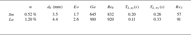
a). The column is filled with tap water to height 90 cm. The distance between opposite walls is 11.5 cm, and all measurements are taken at height 50 cm to ensure that the bubbles are rising at their terminal velocity. Air bubbles are injected through needle spargers at the bottom, and two bubble sizes (3.5 mm and 4.4 mm) are considered in the present work by using spargers with different inner diameters. The gas injection rate of all eight spargers is adjusted to produce nearly homogeneous, monodisperse bubbly flows in the column core. For comparison, we also perform single-bubble experiments with the same corresponding bubble size. Only one sparger is operated at a very low flow rate to produce bubbles that are suffciently separated for them to be considered individual (i.e. they experience negligible flow disturbance due to the other bubbles, and bubble–bubble interactions do not occur). In total, we investigate four different cases, denoted as Sm, La, Sm-Sin and La-Sin (see supplementary movies for each individual case). Here, Sm/La refer to bubbles with mean equivalent diameters approximately 3.5 mm and 4.4 mm, respectively, which we refer to as the smaller and larger bubbles for brevity. The suffix -Sin indicates the corresponding single-bubble cases. Some key parameters of the two bubble swarm cases are summarised in table 1. The measurement set-up and data acquisition are similar to those in our previous work (Ma et al. Reference Ma, Tan, Ni, Hessenkemper and Bragg2025), so only the key aspects for 3D-LBT and 3D-LPT are presented below. The Taylor Reynolds number $Re_\lambda =\sqrt {15/(\nu \varepsilon )}\,u^2_{rms}$
is calculated based on all tracer tracks. Here, the root mean square liquid velocity fluctuation is
$Re_\lambda =\sqrt {15/(\nu \varepsilon )}\,u^2_{rms}$
is calculated based on all tracer tracks. Here, the root mean square liquid velocity fluctuation is $u_{rms}\equiv \sqrt {({1}/{3}) ( \sigma ^2(u_l) + \sigma ^2(v_l) + \sigma ^2(w_l) )}$
, and the turbulence dissipation rate
$u_{rms}\equiv \sqrt {({1}/{3}) ( \sigma ^2(u_l) + \sigma ^2(v_l) + \sigma ^2(w_l) )}$
, and the turbulence dissipation rate $\varepsilon$
is obtained from the compensated structure function (see Ma et al. Reference Ma, Tan, Ni, Hessenkemper and Bragg2025).
$\varepsilon$
is obtained from the compensated structure function (see Ma et al. Reference Ma, Tan, Ni, Hessenkemper and Bragg2025).
Table 1. Selected parameters of the two bubble swarm cases. Here, $\alpha$
denotes the gas void fraction,
$\alpha$
denotes the gas void fraction, $d_b$
is the bubble diameter,
$d_b$
is the bubble diameter, $Eo\equiv (\rho _l-\rho _g)gd^2_b/\sigma$
is the Eötvös number (where
$Eo\equiv (\rho _l-\rho _g)gd^2_b/\sigma$
is the Eötvös number (where $\sigma$
is the surface tension),
$\sigma$
is the surface tension), $Ga\equiv \sqrt {gd^3_b}/\nu$
is the Galileo number, and
$Ga\equiv \sqrt {gd^3_b}/\nu$
is the Galileo number, and $Re_b$
is the bubble Reynolds number based on the bubble-to-fluid relative velocity obtained from the experiment. For the liquid phase,
$Re_b$
is the bubble Reynolds number based on the bubble-to-fluid relative velocity obtained from the experiment. For the liquid phase, $T_{L,u_l}$
and
$T_{L,u_l}$
and $T_{L,w_l}$
are the horizontal and vertical Lagrangian integral time scales computed from their respective autocorrelation functions, and
$T_{L,w_l}$
are the horizontal and vertical Lagrangian integral time scales computed from their respective autocorrelation functions, and $Re_{\lambda }$
is the Taylor Reynolds number.
$Re_{\lambda }$
is the Taylor Reynolds number.
Four high-speed cameras arranged in a linear configuration are employed to capture the 3-D dispersion of bubbles and tracers, with the flow being back-illuminated by LEDs for shadowgraph imaging. The region of interest (ROI) for bubble tracking is $5\times 5\times 15$
cm
$5\times 5\times 15$
cm $^3$
, with recording rate 500 fps. Bubbles are identified and tracked using our in-house 3D-LBT tool (Hessenkemper et al. Reference Hessenkemper, Wang, Lucas, Tan, Ni and Ma2024), specifically designed for tracking relatively dense, deformable bubbles that partially overlap with others in the images. For each case, we collect over
$^3$
, with recording rate 500 fps. Bubbles are identified and tracked using our in-house 3D-LBT tool (Hessenkemper et al. Reference Hessenkemper, Wang, Lucas, Tan, Ni and Ma2024), specifically designed for tracking relatively dense, deformable bubbles that partially overlap with others in the images. For each case, we collect over $2\,00\,000$
bubble tracks and
$2\,00\,000$
bubble tracks and $6\,00\,000$
tracer tracks to ensure statistical convergence. To capture the 3-D flow information, we seed the water with 100
$6\,00\,000$
tracer tracks to ensure statistical convergence. To capture the 3-D flow information, we seed the water with 100 $\unicode{x03BC}$
m polyamide particles as tracers. Since these tracer particles are significantly smaller than bubbles, we perform separate measurements for tracers, with a different ROI
$\unicode{x03BC}$
m polyamide particles as tracers. Since these tracer particles are significantly smaller than bubbles, we perform separate measurements for tracers, with a different ROI $4.5\times 4.5\times 9.0$
cm
$4.5\times 4.5\times 9.0$
cm $^3$
, at frame rate 2500 fps, ensuring sufficient spatio-temporal resolution for the flow. The tracers are tracked in three dimensions using OpenLPT (Tan et al. Reference Tan, Salibindla, Masuk and Ni2020) – an open-source version of the shake-the-box approach (Schanz, Gesemann & Schröder Reference Schanz, Gesemann and Schröder2016) that can handle high particle image densities.
$^3$
, at frame rate 2500 fps, ensuring sufficient spatio-temporal resolution for the flow. The tracers are tracked in three dimensions using OpenLPT (Tan et al. Reference Tan, Salibindla, Masuk and Ni2020) – an open-source version of the shake-the-box approach (Schanz, Gesemann & Schröder Reference Schanz, Gesemann and Schröder2016) that can handle high particle image densities.
Figure 1(b) presents all components of the standard deviation of the bubble fluctuating velocities for all four cases, as well as the standard deviation of the liquid velocities for the two swarm cases. Consistent with previous studies (Lu & Tryggvason Reference Lu and Tryggvason2013), the liquid velocity fluctuations in both Sm and La are anisotropic, with larger fluctuations in the vertical direction (corresponding to the direction of the mean bubble motion). In contrast, the bubble velocity fluctuations in all four cases are larger in the horizontal direction, which we will discuss in detail in § 3.1.
3. Results
3.1. Dispersion of bubble swarms versus single bubbles
Although the asymptotic results in (1.2) were derived for tracer particles, they are based on the kinematic equation $\dot {\boldsymbol{x}}(t)\equiv \boldsymbol{u}_l(t)$
and make no assumption about the dynamics of the particles or flow. As such, exactly the same predictions apply to the case of bubbles dispersing in turbulence, but with
$\dot {\boldsymbol{x}}(t)\equiv \boldsymbol{u}_l(t)$
and make no assumption about the dynamics of the particles or flow. As such, exactly the same predictions apply to the case of bubbles dispersing in turbulence, but with $\sigma (u_l)$
replaced by
$\sigma (u_l)$
replaced by $\sigma (u_b)$
, and
$\sigma (u_b)$
, and $T_{L,u_l}$
replaced by
$T_{L,u_l}$
replaced by $T_{L,u_b}$
.
$T_{L,u_b}$
.
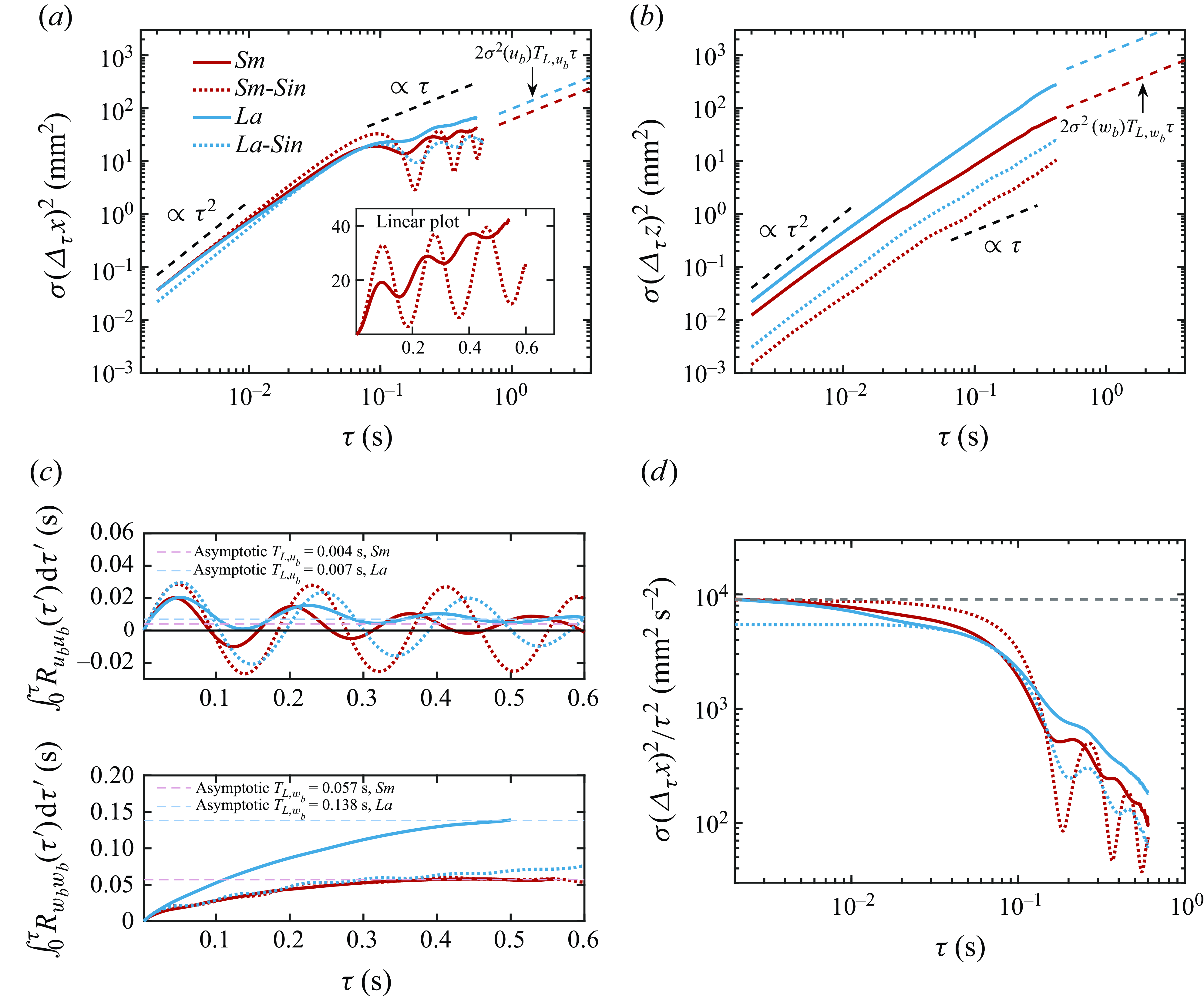
Figure 2. The MSD for single bubbles (dashed lines) and bubble swarms (solid lines) in the (a) horizontal and (b) vertical directions. Dashed lines indicate asymptotic MSD for long-time diffusive behaviour. (c) Integral of Lagrangian autocorrelation function of bubble velocity in the horizontal and vertical components, respectively. Here, $T_{L,u_b}$
and
$T_{L,u_b}$
and $T_{L,w_b}$
are estimated from the asymptotic value of the curve (dashed lines). (d) Horizontal MSD compensated by
$T_{L,w_b}$
are estimated from the asymptotic value of the curve (dashed lines). (d) Horizontal MSD compensated by $\tau ^2$
to emphasise the deviation from the ballistic regime with increasing time.
$\tau ^2$
to emphasise the deviation from the ballistic regime with increasing time.
From the 3-D bubble tracks, we compute the horizontal (figure 2
a) and vertical (figure 2
b) components of the MSD for the bubbles as a function of time lag $\tau$
for all four cases. For small
$\tau$
for all four cases. For small $\tau$
, the MSDs of both bubble swarms (Sm/La) and single bubbles (Sm-Sin/La-Sin) exhibit a
$\tau$
, the MSDs of both bubble swarms (Sm/La) and single bubbles (Sm-Sin/La-Sin) exhibit a $\tau ^2$
growth in both directions, as bubbles essentially follow a ballistic motion. This ballistic motion occurs because for
$\tau ^2$
growth in both directions, as bubbles essentially follow a ballistic motion. This ballistic motion occurs because for $\tau$
much smaller than the correlation time scale of the fluctuating bubble velocities, the bubble velocities are constant to leading order in
$\tau$
much smaller than the correlation time scale of the fluctuating bubble velocities, the bubble velocities are constant to leading order in $\tau$
. For the vertical direction, we find that the MSD for bubble swarms is much larger than that for single bubbles (figure 2
b). This difference is due to the BIT experienced by the bubbles dispersing in swarms, and the anisotropy of this BIT. It is known that rising bubble swarms generate larger vertical than horizontal fluctuating velocities in the flow (Riboux, Risso & Legendre Reference Riboux, Risso and Legendre2010), with ratios
$\tau$
. For the vertical direction, we find that the MSD for bubble swarms is much larger than that for single bubbles (figure 2
b). This difference is due to the BIT experienced by the bubbles dispersing in swarms, and the anisotropy of this BIT. It is known that rising bubble swarms generate larger vertical than horizontal fluctuating velocities in the flow (Riboux, Risso & Legendre Reference Riboux, Risso and Legendre2010), with ratios $\sigma (w_l)/\sigma (u_l)$
of 1.33 and 1.45 for the Sm and La cases, respectively. Related to this,
$\sigma (w_l)/\sigma (u_l)$
of 1.33 and 1.45 for the Sm and La cases, respectively. Related to this, $\sigma (w_b)$
is much larger for bubble swarms than single-bubbles due to the BIT, and
$\sigma (w_b)$
is much larger for bubble swarms than single-bubbles due to the BIT, and $\sigma (w_b)$
is approximately three times greater for the swarm cases than the corresponding single-bubble cases (see figure 1
b). Since the vertical MSD is proportional to
$\sigma (w_b)$
is approximately three times greater for the swarm cases than the corresponding single-bubble cases (see figure 1
b). Since the vertical MSD is proportional to $\sigma ^2(w_b)$
, this results in an order of magnitude increase in the vertical MSD of bubble swarms compared with single bubbles in the ballistic regime. In contrast, the horizontal component of the MSD does not show such significant differences, since the variations in
$\sigma ^2(w_b)$
, this results in an order of magnitude increase in the vertical MSD of bubble swarms compared with single bubbles in the ballistic regime. In contrast, the horizontal component of the MSD does not show such significant differences, since the variations in $\sigma (u_b)$
(or
$\sigma (u_b)$
(or $\sigma (v_b)$
) between the single-bubble and swarm cases are relatively small. This is because the horizontal fluctuations of the bubble velocity are dominated by wake-induced instabilities that are common to both the single-bubble and swarm cases.
$\sigma (v_b)$
) between the single-bubble and swarm cases are relatively small. This is because the horizontal fluctuations of the bubble velocity are dominated by wake-induced instabilities that are common to both the single-bubble and swarm cases.
As $\tau$
increases, the MSD gradually deviates from the ballistic behaviour. The most striking behaviour is for the horizontal direction (figure 2
a); for the two single-bubble cases, the MSD oscillates strongly, while for the swarm cases, although the oscillations in the MSD are present (the linear inset plot shows this more clearly), they are strongly damped. The oscillations in the MSD for the Sm-Sin and La-Sin cases occurs due to the wake instability that leads to an oscillatory rising path for the bubbles (Cano-Lozano et al. Reference Cano-Lozano, Martinez-Bazan, Magnaudet and Tchoufag2016; Legendre & Zenit Reference Legendre and Zenit2025). For the two swarm cases, the MSD oscillations are much weaker because the chaotic effects of BIT and bubble–bubble interactions suppress the systematic oscillatory motion. The oscillations are in fact almost unnoticeable for the La case, where higher BIT and stronger bubble–bubble interactions further suppress the oscillations compared to the Sm case. Interestingly, the damped MSD oscillations share similarities with those observed for active self-propelled particles moving at the air–water interface in a Petri dish (Bourgoin et al. Reference Bourgoin, Kervil, Cottin-Bizonne, Raynal, Volk and Ybert2020). In that case, the oscillatory MSD of a single active particle is damped with increasing particle number due to the particle interactions, paving the way for a diffusive MSD behaviour. Although the origin of the oscillations in the MSD is different for the isolated active particle studied in Bourgoin et al. (Reference Bourgoin, Kervil, Cottin-Bizonne, Raynal, Volk and Ybert2020) (where it is caused by reorientation of the particle trajectory upon hitting the dish boundary) and for an isolated bubble in the present study (where it is caused by wake instabilities), the attenuation of the oscillations with increasing particle/bubble number in both situations reflects the randomising effect of the collective motion on the individual particle/bubble motion.
$\tau$
increases, the MSD gradually deviates from the ballistic behaviour. The most striking behaviour is for the horizontal direction (figure 2
a); for the two single-bubble cases, the MSD oscillates strongly, while for the swarm cases, although the oscillations in the MSD are present (the linear inset plot shows this more clearly), they are strongly damped. The oscillations in the MSD for the Sm-Sin and La-Sin cases occurs due to the wake instability that leads to an oscillatory rising path for the bubbles (Cano-Lozano et al. Reference Cano-Lozano, Martinez-Bazan, Magnaudet and Tchoufag2016; Legendre & Zenit Reference Legendre and Zenit2025). For the two swarm cases, the MSD oscillations are much weaker because the chaotic effects of BIT and bubble–bubble interactions suppress the systematic oscillatory motion. The oscillations are in fact almost unnoticeable for the La case, where higher BIT and stronger bubble–bubble interactions further suppress the oscillations compared to the Sm case. Interestingly, the damped MSD oscillations share similarities with those observed for active self-propelled particles moving at the air–water interface in a Petri dish (Bourgoin et al. Reference Bourgoin, Kervil, Cottin-Bizonne, Raynal, Volk and Ybert2020). In that case, the oscillatory MSD of a single active particle is damped with increasing particle number due to the particle interactions, paving the way for a diffusive MSD behaviour. Although the origin of the oscillations in the MSD is different for the isolated active particle studied in Bourgoin et al. (Reference Bourgoin, Kervil, Cottin-Bizonne, Raynal, Volk and Ybert2020) (where it is caused by reorientation of the particle trajectory upon hitting the dish boundary) and for an isolated bubble in the present study (where it is caused by wake instabilities), the attenuation of the oscillations with increasing particle/bubble number in both situations reflects the randomising effect of the collective motion on the individual particle/bubble motion.
At the largest time for which the MSD is computed $\tau =\tau _{max}$
, the behaviour does not actually follow a diffusive behaviour
$\tau =\tau _{max}$
, the behaviour does not actually follow a diffusive behaviour $\propto \tau$
. The data in figure 2(c) indicate that this is because the integral of the bubble velocity autocorrelation over the time span
$\propto \tau$
. The data in figure 2(c) indicate that this is because the integral of the bubble velocity autocorrelation over the time span $[0,\tau ]$
does not converge to a constant as
$[0,\tau ]$
does not converge to a constant as $\tau \to \tau _{max}$
(although it almost converges for the vertical components). For the swarm cases, the integral oscillates about a mean value with amplitude that decreases with increasing
$\tau \to \tau _{max}$
(although it almost converges for the vertical components). For the swarm cases, the integral oscillates about a mean value with amplitude that decreases with increasing $\tau$
. We can estimate the integral time scale from the asymptotic value of the curve at large
$\tau$
. We can estimate the integral time scale from the asymptotic value of the curve at large $\tau$
, and using these we show in figure 2(a,b) the diffusive behaviour (e.g.
$\tau$
, and using these we show in figure 2(a,b) the diffusive behaviour (e.g. $\sigma ^2(\varDelta _{\tau }x)=2\sigma ^2(u_b)\, T_{L,u_b}\tau$
) that would be expected for time larger than
$\sigma ^2(\varDelta _{\tau }x)=2\sigma ^2(u_b)\, T_{L,u_b}\tau$
) that would be expected for time larger than $\tau _{max}$
for the swarm cases. These indicate that the MSD is in fact approaching the expected diffusive behaviour. For the single-bubble cases, the amplitude of the oscillations of the integrals decreases very slowly with time. Assuming that the integrals would eventually converge, this indicates that extremely large times are required to observe diffusive growth for the single-bubble cases.
$\tau _{max}$
for the swarm cases. These indicate that the MSD is in fact approaching the expected diffusive behaviour. For the single-bubble cases, the amplitude of the oscillations of the integrals decreases very slowly with time. Assuming that the integrals would eventually converge, this indicates that extremely large times are required to observe diffusive growth for the single-bubble cases.
We note that the transition away from the ballistic regime occurs earlier for the swarm cases, which can be better seen in the compensated horizontal MSD in figure 2(d). In the swarm cases, bubbles maintain their initial velocity for less time than single bubbles due to the randomising effects of BIT and hydrodynamic interactions with other bubbles in their vicinity.
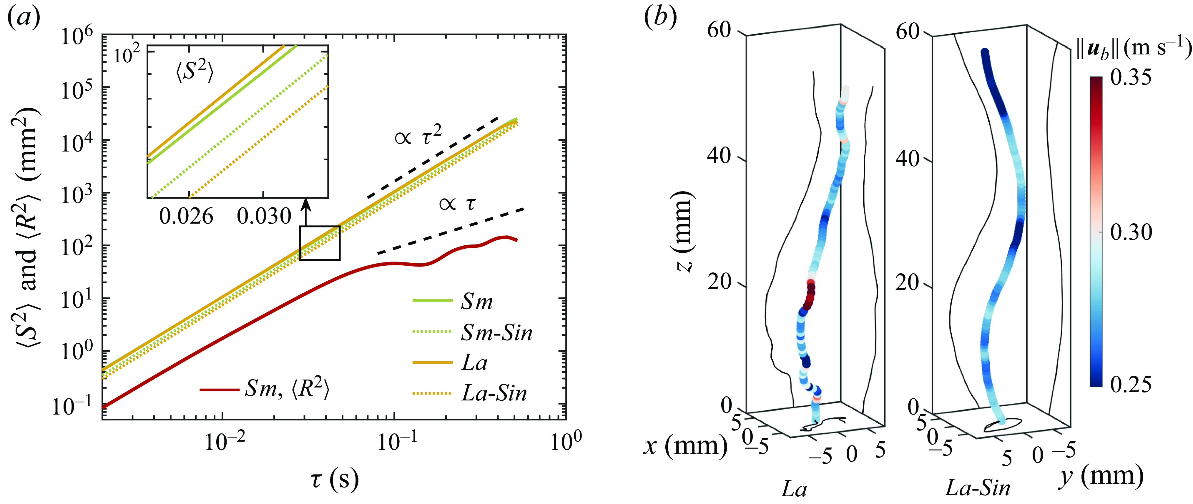
Figure 3. (a) Mean squared path length $\langle S^2 \rangle$
, together with the total MSD
$\langle S^2 \rangle$
, together with the total MSD $\langle R^2 \rangle$
of Sm as comparison. (b) Snapshots of typical bubble trajectories for La and La-Sin, with the same tracking time. The trajectories are coloured by the magnitude of the total velocity
$\langle R^2 \rangle$
of Sm as comparison. (b) Snapshots of typical bubble trajectories for La and La-Sin, with the same tracking time. The trajectories are coloured by the magnitude of the total velocity $\|\boldsymbol{u}_b \|$
.
$\|\boldsymbol{u}_b \|$
.
3.2. Path length of bubble swarms versus single bubbles
While the MSD provides a simple metric for understanding the bubble dispersion, further information can be found by studying the path length $S(\tau )$
of the trajectories (Ouellette, Bodenschatz & Xu Reference Ouellette, Bodenschatz and Xu2011), i.e. the total distance travelled by individual bubbles. We can approximately measure the mean-squared path length using
$S(\tau )$
of the trajectories (Ouellette, Bodenschatz & Xu Reference Ouellette, Bodenschatz and Xu2011), i.e. the total distance travelled by individual bubbles. We can approximately measure the mean-squared path length using
 \begin{equation} \langle S^2(\tau ) \rangle \approx \left \langle \bigg[ \sum _{\gamma =1}^{N_{\tau }} \left \| \boldsymbol{x}(t_0 + \gamma\, \varDelta t) - \boldsymbol{x}(t_0 + [\gamma - 1]\, \varDelta t) \right \|\bigg]^2 \right \rangle , \end{equation}
where $N_\tau \equiv 1+(\tau -t_0)/\varDelta t \in \mathbb{Z}^+$
, and
$N_\tau \equiv 1+(\tau -t_0)/\varDelta t \in \mathbb{Z}^+$
, and $\varDelta t=0.002\ \text{s}$
is used based on our imaging rate for tracking bubbles. For a representative case Sm, we plot
$\varDelta t=0.002\ \text{s}$
is used based on our imaging rate for tracking bubbles. For a representative case Sm, we plot $\langle S^2\rangle$
in figure 3(a), alongside the total MSD
$\langle S^2\rangle$
in figure 3(a), alongside the total MSD $\langle R^2(\tau ) \rangle$
based on all three components of
$\langle R^2(\tau ) \rangle$
based on all three components of $\boldsymbol{x}$
:
$\boldsymbol{x}$
:
 \begin{equation} \langle R^2(\tau ) \rangle \equiv \langle ||\varDelta _{\tau }\boldsymbol{x} - \langle \varDelta _{\tau }\boldsymbol{x}\rangle ||^2\rangle . \end{equation}
The other case, La, shows similar behaviour so is not shown here. For both single bubbles and bubble swarms, $\langle S^2\rangle$
grows as
$\langle S^2\rangle$
grows as $\tau ^2$
over almost the entire trajectory, differing from
$\tau ^2$
over almost the entire trajectory, differing from $\langle R^2\rangle$
, which undergoes a transition towards a diffusive growth at long times. We see a vertical shift between
$\langle R^2\rangle$
, which undergoes a transition towards a diffusive growth at long times. We see a vertical shift between $\langle S^2\rangle$
and
$\langle S^2\rangle$
and $\langle R^2\rangle$
in the short term due to the subtraction of mean displacement by computing
$\langle R^2\rangle$
in the short term due to the subtraction of mean displacement by computing $\langle R^2 \rangle$
in (3.2). (As an aside, in Ouellette et al. (Reference Ouellette, Bodenschatz and Xu2011),
$\langle R^2 \rangle$
in (3.2). (As an aside, in Ouellette et al. (Reference Ouellette, Bodenschatz and Xu2011), $\langle S^2\rangle \approx \langle R^2\rangle$
for the short-time ballistic regime, since in their flow there is no mean displacement for the tracer particles.) The zoomed-in view of
$\langle S^2\rangle \approx \langle R^2\rangle$
for the short-time ballistic regime, since in their flow there is no mean displacement for the tracer particles.) The zoomed-in view of $\langle S^2\rangle$
(inset of figure 3
a) shows that the path travelled by bubbles rising in swarms is longer than that for the single-bubble cases. This may seem counter-intuitive at first, as it has been found that bubbles rising in turbulence have a reduced rise velocity compared to those in a quiescent liquid (Loisy & Naso Reference Loisy and Naso2017; Ruth et al. Reference Ruth, Vernet, Perrard and Deike2021). The explanation for this is that the path length is determined by
$\langle S^2\rangle$
(inset of figure 3
a) shows that the path travelled by bubbles rising in swarms is longer than that for the single-bubble cases. This may seem counter-intuitive at first, as it has been found that bubbles rising in turbulence have a reduced rise velocity compared to those in a quiescent liquid (Loisy & Naso Reference Loisy and Naso2017; Ruth et al. Reference Ruth, Vernet, Perrard and Deike2021). The explanation for this is that the path length is determined by $\left\langle \left \| \boldsymbol{u}_b \right \|\right\rangle = \langle \sqrt {u_b^2+v_b^2+w_b^2}\rangle$
, and not the rise velocity. Indeed, the exact expression for the path length is
$\left\langle \left \| \boldsymbol{u}_b \right \|\right\rangle = \langle \sqrt {u_b^2+v_b^2+w_b^2}\rangle$
, and not the rise velocity. Indeed, the exact expression for the path length is $ S(\tau ) = \int _0^\tau \|\boldsymbol{u}_b(s)\|\,{\rm d}s$
, and for statistically stationary bubble tracks and large
$ S(\tau ) = \int _0^\tau \|\boldsymbol{u}_b(s)\|\,{\rm d}s$
, and for statistically stationary bubble tracks and large $\tau$
, we have
$\tau$
, we have $S(\tau )\approx \tau \langle \|\boldsymbol{u}_b\|\rangle$
. The measured
$S(\tau )\approx \tau \langle \|\boldsymbol{u}_b\|\rangle$
. The measured $\langle \left \| \boldsymbol{u}_b \right \|\rangle$
is 0.315 m s−1 for Sm, 0.286 m s−1 for Sm-Sin, 0.319 m s−1 for La, and 0.269 m s−1 for La-Sin. This corresponds to 10.2 % and 18.7 % increases in path length for Sm and La, respectively, compared to their single-bubble cases. For illustration, we show representative trajectories of La and La-Sin in figure 3(b). Bubbles in swarms have smaller vertical displacements due to decreasing rise velocity, but more twisted trajectories. The figures also indicate that the rising paths of bubbles in swarms still exhibit oscillations, and this is due to the intrinsic wake-driven dynamics dominating the low-frequency behaviour of the bubble motion. However, higher-frequency motion is more erratic and reflects the effect of BIT at small scales in the flow.
$\langle \left \| \boldsymbol{u}_b \right \|\rangle$
is 0.315 m s−1 for Sm, 0.286 m s−1 for Sm-Sin, 0.319 m s−1 for La, and 0.269 m s−1 for La-Sin. This corresponds to 10.2 % and 18.7 % increases in path length for Sm and La, respectively, compared to their single-bubble cases. For illustration, we show representative trajectories of La and La-Sin in figure 3(b). Bubbles in swarms have smaller vertical displacements due to decreasing rise velocity, but more twisted trajectories. The figures also indicate that the rising paths of bubbles in swarms still exhibit oscillations, and this is due to the intrinsic wake-driven dynamics dominating the low-frequency behaviour of the bubble motion. However, higher-frequency motion is more erratic and reflects the effect of BIT at small scales in the flow.
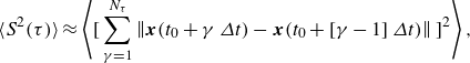
3.3. Probability density function of fluctuating bubble velocity of bubble swarms versus single bubbles
To fully understand the bubble motion as they disperse, we now turn to consider the probability density functions (PDFs) of the fluctuating bubble velocities, $\boldsymbol{u}'_b=\boldsymbol{u}_b-\langle \boldsymbol{u}_b\rangle$
, in figure 4. In the horizontal direction, both single bubbles and bubble swarms have symmetric and non-Gaussian PDFs. For the two single-bubble cases, while the PDF of Sm-Sin is bi-modal, La-Sin is uni-modal with a peak that is wide and flat compared to a Gaussian PDF. These features can also be related to the oscillations in their trajectories, with the stronger oscillations of the MSD for the case Sm-Sin (figure 2
a) being associated with a clear bi-modal velocity PDF. Similar behaviour was also reported by Mathai et al. (Reference Mathai, Prakash, Brons, Sun and Lohse2015) for finite-sized buoyant particles. For the corresponding swarm cases, the BIT and bubble–bubble interactions introduce additional randomness into the bubble motion, leading to Gaussian-like behaviour in the central region of the PDFs. However, the PDFs have tails that are heavier than in a Gaussian PDF, while those for single bubbles are lighter, indicating intermittency due to the collective motion of the bubbles in swarms. Such intermittent bubble velocities have been observed previously (Ma et al. Reference Ma, Hessenkemper, Lucas and Bragg2023), and may arise when a trailing bubble is caught in the wake of leading bubbles, or be due to intense hydrodynamic interactions between bubbles when they become sufficiently close.
$\boldsymbol{u}'_b=\boldsymbol{u}_b-\langle \boldsymbol{u}_b\rangle$
, in figure 4. In the horizontal direction, both single bubbles and bubble swarms have symmetric and non-Gaussian PDFs. For the two single-bubble cases, while the PDF of Sm-Sin is bi-modal, La-Sin is uni-modal with a peak that is wide and flat compared to a Gaussian PDF. These features can also be related to the oscillations in their trajectories, with the stronger oscillations of the MSD for the case Sm-Sin (figure 2
a) being associated with a clear bi-modal velocity PDF. Similar behaviour was also reported by Mathai et al. (Reference Mathai, Prakash, Brons, Sun and Lohse2015) for finite-sized buoyant particles. For the corresponding swarm cases, the BIT and bubble–bubble interactions introduce additional randomness into the bubble motion, leading to Gaussian-like behaviour in the central region of the PDFs. However, the PDFs have tails that are heavier than in a Gaussian PDF, while those for single bubbles are lighter, indicating intermittency due to the collective motion of the bubbles in swarms. Such intermittent bubble velocities have been observed previously (Ma et al. Reference Ma, Hessenkemper, Lucas and Bragg2023), and may arise when a trailing bubble is caught in the wake of leading bubbles, or be due to intense hydrodynamic interactions between bubbles when they become sufficiently close.
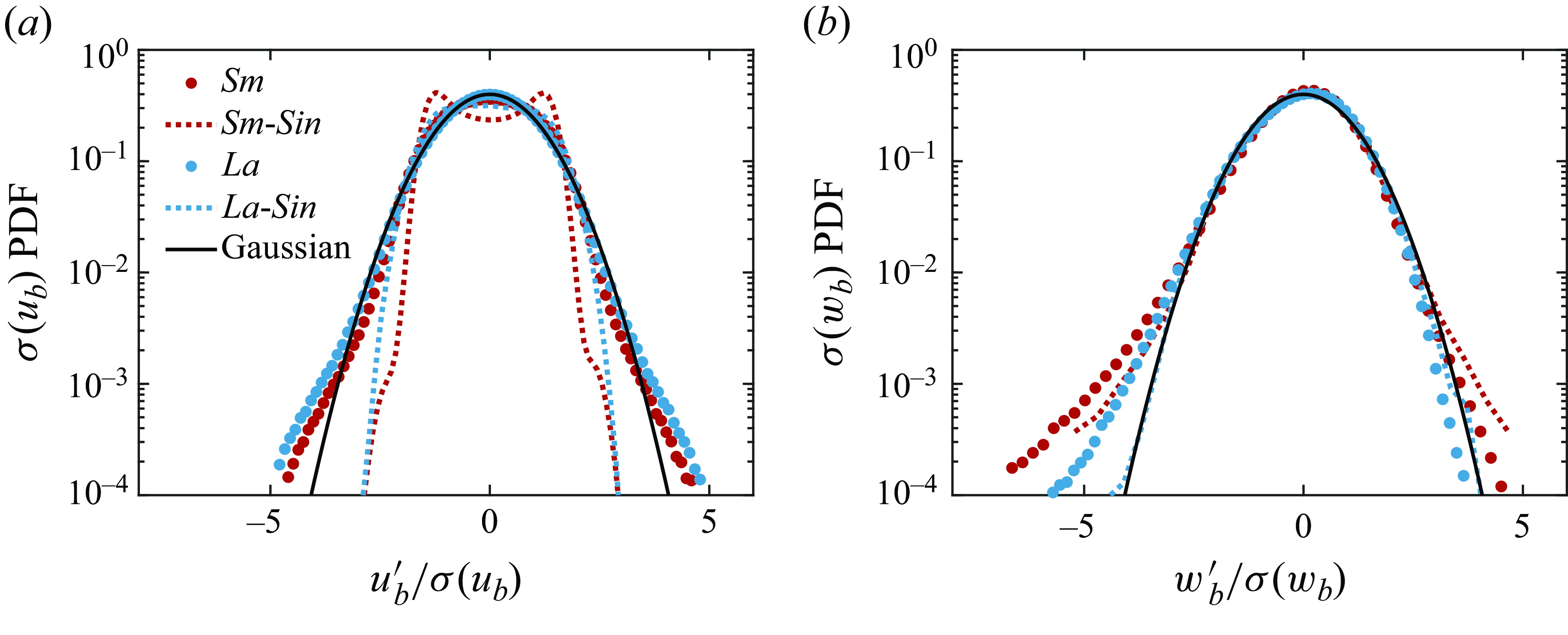
Figure 4. The PDFs of the fluctuating bubble velocities in the (a) horizontal and (b) vertical directions, normalised by their standard deviations $\sigma (u_b)$
and
$\sigma (u_b)$
and $\sigma (w_b)$
, respectively.
$\sigma (w_b)$
, respectively.
In the vertical direction (figure 4 b), the PDFs of Sm and La are negatively skewed, unlike their corresponding single-bubble cases for which the PDFs are approximately symmetric. The negative skewness in the swarm cases is consistent with our previous study (Ma et al. Reference Ma, Hessenkemper, Lucas and Bragg2023) and the observation in Martínez et al. (Reference Martínez, Chehata, van Gils, Sun and Lohse2010). For bubble swarms, Ma et al. (Reference Ma, Hessenkemper, Lucas and Bragg2023) argued that the PDF of bubble vertical velocity fluctuations can exhibit skewness of either sign, depending in a complex way on the background turbulence and additional factors, such as the bubble size relative to the turbulence length scales.
3.4. Dispersion of bubble swarms versus liquid tracers
We finally turn our attention to the difference in dispersion between bubbles and liquid tracers in the swarm cases, and figure 5(a,b) show their horizontal and vertical MSDs, respectively. At short times, the horizontal dispersion of bubbles is almost an order of magnitude faster than that of tracers, whereas the difference in their MSD in the vertical direction is smaller. This can be attributed to the relative difference between the fluctuating bubble velocity and fluctuating liquid velocity, and how this difference varies in the horizontal and vertical directions (see figure 1(b) for the Sm and La cases). More specifically, the horizontal components $\sigma (u_b)$
and
$\sigma (u_b)$
and $\sigma (v_b)$
are significantly larger than the corresponding ones for the liquid,
$\sigma (v_b)$
are significantly larger than the corresponding ones for the liquid, $\sigma (u_l)$
and
$\sigma (u_l)$
and $\sigma (v_l)$
. In contrast, the difference between the vertical components
$\sigma (v_l)$
. In contrast, the difference between the vertical components $\sigma (w_b)$
and
$\sigma (w_b)$
and $\sigma (w_l)$
is much smaller, leading to more similar ballistic dispersion between the two phases (figure 5
b). At longer times, the horizontal MSD of bubbles approaches (but does not actually attain, due to the limited
$\sigma (w_l)$
is much smaller, leading to more similar ballistic dispersion between the two phases (figure 5
b). At longer times, the horizontal MSD of bubbles approaches (but does not actually attain, due to the limited $\tau _{max}$
, as discussed earlier) a diffusive-like regime
$\tau _{max}$
, as discussed earlier) a diffusive-like regime $\propto \tau$
, while the MSD for tracers does not. This is simply due to
$\propto \tau$
, while the MSD for tracers does not. This is simply due to $\tau _{max}$
being too small to observe this regime for the tracers. However, the plots show the diffusive prediction for the tracers, and these indicate that the diffusive regime would be reached if
$\tau _{max}$
being too small to observe this regime for the tracers. However, the plots show the diffusive prediction for the tracers, and these indicate that the diffusive regime would be reached if $\tau _{max}$
were several times larger.
$\tau _{max}$
were several times larger.
Figure 5. MSD for bubbles and fluid tracers in the (a) horizontal and (b) vertical directions. Dashed lines indicate the asymptotic dispersion rate for long-time diffusive behaviour. Compensated horizontal MSD for the (c) Sm and (d) La cases. The solid vertical lines indicate the onset of transition for bubbles, while the dashed vertical line marks the transition for tracers, defined as the time when the local exponential decay reaches 80 %. For Sm, the bubble transition occurs at a similar time, so only one vertical line is shown.
With increasing $\tau$
, the MSD for the tracers gradually exceeds that for the bubbles, in agreement with the results of Mathai et al. (Reference Mathai, Huisman, Sun, Lohse and Bourgoin2018) for isolated smaller bubbles in HIT. Mathai et al. (Reference Mathai, Huisman, Sun, Lohse and Bourgoin2018) explained this as being due to the crossing-trajectory effect, whereby bubbles can drift through turbulent eddies due to their buoyant rising motion, causing the fluid velocities along their trajectories to decorrelate more rapidly than along tracer trajectories. This mechanism is plausible for their experiments where the bubbles are rising through pre-existing background turbulence and eddies. However, its role in our experiments is less clear, because in ours the bubbles are not rising through pre-existing turbulent eddies, but are in fact generating the eddies themselves as they rise. In our case, what is clear is that the longer correlation time scale for the tracers means that the faster ballistic growth persists for longer for tracers than for bubbles, enabling their dispersion to overtake that of the bubbles. The crossing-trajectory effect may contribute to the reason why the correlation time scale is longer for tracers, but it could also be due to fluctuations associated with the bubble wakes causing the bubble velocities to decorrelate faster than those of tracers, which do not generate fluctuating wakes due to the low Reynolds number of the tracers.
$\tau$
, the MSD for the tracers gradually exceeds that for the bubbles, in agreement with the results of Mathai et al. (Reference Mathai, Huisman, Sun, Lohse and Bourgoin2018) for isolated smaller bubbles in HIT. Mathai et al. (Reference Mathai, Huisman, Sun, Lohse and Bourgoin2018) explained this as being due to the crossing-trajectory effect, whereby bubbles can drift through turbulent eddies due to their buoyant rising motion, causing the fluid velocities along their trajectories to decorrelate more rapidly than along tracer trajectories. This mechanism is plausible for their experiments where the bubbles are rising through pre-existing background turbulence and eddies. However, its role in our experiments is less clear, because in ours the bubbles are not rising through pre-existing turbulent eddies, but are in fact generating the eddies themselves as they rise. In our case, what is clear is that the longer correlation time scale for the tracers means that the faster ballistic growth persists for longer for tracers than for bubbles, enabling their dispersion to overtake that of the bubbles. The crossing-trajectory effect may contribute to the reason why the correlation time scale is longer for tracers, but it could also be due to fluctuations associated with the bubble wakes causing the bubble velocities to decorrelate faster than those of tracers, which do not generate fluctuating wakes due to the low Reynolds number of the tracers.
In figure 5(c,d), we plot the compensated horizontal MSD for both phases, and find that for both Sm and La, the time span of the ballistic regime is set by the wake-induced motion at a bubble time scale $O(d_b/\left \langle w_b \right \rangle )$
(Ma et al. Reference Ma, Santarelli, Ziegenhein, Lucas and Fröhlich2017, Reference Ma, Lucas, Jakirlić and Fröhlich2020), approximately 0.01 s. However, the time span for the tracers is different for the Sm and La cases. For the La case, the transition away from the ballistic regime occurs considerably later for the tracers than for the bubbles for the La case. This confirms the finding of Mathai et al. (Reference Mathai, Huisman, Sun, Lohse and Bourgoin2018) that the transition for bubbles occurs much earlier than for tracer particles due to their oscillatory wake-driven dynamics. By contrast, for the Sm case, the transition for bubbles and tracers occurs at the same time (see figure 5
c). The explanation is that for the Sm case, where
$O(d_b/\left \langle w_b \right \rangle )$
(Ma et al. Reference Ma, Santarelli, Ziegenhein, Lucas and Fröhlich2017, Reference Ma, Lucas, Jakirlić and Fröhlich2020), approximately 0.01 s. However, the time span for the tracers is different for the Sm and La cases. For the La case, the transition away from the ballistic regime occurs considerably later for the tracers than for the bubbles for the La case. This confirms the finding of Mathai et al. (Reference Mathai, Huisman, Sun, Lohse and Bourgoin2018) that the transition for bubbles occurs much earlier than for tracer particles due to their oscillatory wake-driven dynamics. By contrast, for the Sm case, the transition for bubbles and tracers occurs at the same time (see figure 5
c). The explanation is that for the Sm case, where $\alpha$
is much smaller, there are relatively few regions in the liquid where turbulence is generated by the bubbles, such that turbulence in the flow is very patchy and intermittent. In this case, the tracer dispersion will be highly dependent upon the bubble parameters. For the La case with higher
$\alpha$
is much smaller, there are relatively few regions in the liquid where turbulence is generated by the bubbles, such that turbulence in the flow is very patchy and intermittent. In this case, the tracer dispersion will be highly dependent upon the bubble parameters. For the La case with higher $\alpha$
and larger
$\alpha$
and larger $d_b$
, the bubble wakes are longer, wider and more numerous. As a result, the wake regions are more space filling and wake–wake interactions are more frequent, leading to a flow that is more homogeneous and well mixed (see Ma et al. (Reference Ma, Tan, Ni, Hessenkemper and Bragg2025)). In this respect, the flow in the La case is more similar to that in Mathai et al. (Reference Mathai, Huisman, Sun, Lohse and Bourgoin2018), where there is background turbulence generated by an active grid. This explains the qualitative agreement between the La case and the results of Mathai et al. (Reference Mathai, Huisman, Sun, Lohse and Bourgoin2018) regarding the timing of the departure from the ballistic regime for both tracers and bubbles. However, quantitatively, Mathai et al. (Reference Mathai, Huisman, Sun, Lohse and Bourgoin2018) observe the bubbles departing from the ballistic regime ten times faster than the tracers, whereas in our case it is three times faster. This difference is due to most of the turbulence in their flow being generated by the active grid, whereas in ours it is purely BIT, which is more dependent on the bubble parameters.
$d_b$
, the bubble wakes are longer, wider and more numerous. As a result, the wake regions are more space filling and wake–wake interactions are more frequent, leading to a flow that is more homogeneous and well mixed (see Ma et al. (Reference Ma, Tan, Ni, Hessenkemper and Bragg2025)). In this respect, the flow in the La case is more similar to that in Mathai et al. (Reference Mathai, Huisman, Sun, Lohse and Bourgoin2018), where there is background turbulence generated by an active grid. This explains the qualitative agreement between the La case and the results of Mathai et al. (Reference Mathai, Huisman, Sun, Lohse and Bourgoin2018) regarding the timing of the departure from the ballistic regime for both tracers and bubbles. However, quantitatively, Mathai et al. (Reference Mathai, Huisman, Sun, Lohse and Bourgoin2018) observe the bubbles departing from the ballistic regime ten times faster than the tracers, whereas in our case it is three times faster. This difference is due to most of the turbulence in their flow being generated by the active grid, whereas in ours it is purely BIT, which is more dependent on the bubble parameters.
4. Conclusions
We used experiments equipped with 3D-LBT and 3D-LPT to explore the Taylor dispersion of bubble swarms rising in initially quiescent water. The bubbles considered are large and relatively dense, and their wakes generate significant turbulence and bubble–bubble interactions – a complementary flow condition to that in the previous work by Mathai et al. (Reference Mathai, Huisman, Sun, Lohse and Bourgoin2018). To better understand their Taylor dispersion, we compared: (i) bubble swarms with single bubbles; (ii) bubble swarms with fluid tracers.
For (i), we observe that at long times, the horizontal MSD exhibits oscillations for both the bubble swarms and single-bubble cases. These oscillations are due to wake-induced motion of the bubbles and are, however, strongly damped for the swarm cases compared to the single-bubble cases, primarily due to BIT and bubble–bubble interactions. Due to the damping, the swarm cases approach a diffusive regime, while the single-bubble cases do not. The vertical MSD in bubble swarms is significantly larger than that for the single-bubble cases due to the much higher vertical fluctuating bubble velocity in the swarm cases. We also compute the path length of the rising bubbles, and find that it is up to $18.7\,\%$
larger in swarms than for single bubbles due to BIT, which contorts the trajectories in the swarms.
$18.7\,\%$
larger in swarms than for single bubbles due to BIT, which contorts the trajectories in the swarms.
For (ii), we find a faster dispersion rate in the ballistic regime for bubble swarms than for tracers due to their larger velocities. At longer times, the dispersion of the bubbles is overtaken by the tracers as the faster ballistic regime persists for longer for the tracers. The time to transition away from the ballistic regime is of the order of bubble time scale for smaller and more dilute swarm cases, while the results for larger bubbles with higher gas void fraction reveal an earlier transition for the bubbles compared to the tracers.
Supplementary movies
Supplementary movies are available at https://doi.org/10.1017/jfm.2025.10316.
Funding
We acknowledge financial support from the German Research Foundation (DFG) under grant no. 555712173.
Declaration of interests
The authors report no conflict of interest.


 Open access