


Introduction
Tropical glaciers are highly sensitive to climate change (Kaser, Reference Kaser1999; Cook and others, Reference Cook, Kougkoulos, Edwards, Dortch and Hoffmann2016; Richardson and others, Reference Richardson, Carr and Cook2024). More than 99% of the world’s tropical glaciers are in the Tropical Andes (Vuille and others, Reference Vuille2018), with ∼20% located in Bolivia (Rabatel and others, Reference Rabatel2013). The rate of retreat of Andean glaciers has increased since the 1970s, predominantly driven by rising temperatures (Vuille and others, Reference Vuille2018). Indeed, Gorin and others (Reference Gorin2024) demonstrate that these glaciers now occupy a smaller extent than at any other point during the Holocene. There are several potentially negative and challenging impacts associated with glacier recession in Bolivia. Glacial melt is an important source of freshwater in this region, particularly during the dry season (May to October) when it constitutes up to 24% of freshwater supply to the major city of La Paz (Soruco and others, Reference Soruco2015). A projected reduction in streamflow due to continued glacier retreat is likely to result in negative impacts on water supplies for human consumption, irrigation, hydropower, and industry (Kaenzig, Reference Kaenzig2015; Soruco and others, Reference Soruco2015; Huss and Hock, Reference Huss and Hock2018; Vuille and others, Reference Vuille2018). Reduced streamflow may further result in the desiccation of high-altitude wetlands (‘bofedales’), resulting in diminished biodiversity and a reduction in soil carbon storage (Cuesta and others, Reference Cuesta2019; Cardenas and others, Reference Cardenas2022). Additionally, the shrinkage of Bolivian glaciers may have negative impacts on tourism and indigenous cultural identity, both of which are related to some extent to the presence of glaciers (Kaenzig, Reference Kaenzig2015; Taylor and others, Reference Taylor, Quincey, Smith, Potter, Castro and Fyffe2022).
This study focuses specifically on the implications of glacier recession for glacial lake outburst flood (GLOF) susceptibility in the Bolivian Andes, which has become a growing concern in recent years because of the increase in the number and size of proglacial lakes in the region (Cook and others, Reference Cook, Kougkoulos, Edwards, Dortch and Hoffmann2016; Kougkoulos and others, Reference Kougkoulos2018a, b; Emmer and others, Reference Emmer2022). Carrivick and Tweed (Reference Carrivick and Tweed2013) define proglacial lakes as being influenced directly by either ice margins or subaerial glacial meltwater. They highlight that proglacial lakes can be dammed either by ice, bedrock, moraine, or landslide. We focus on proglacial lakes (henceforth referred to as glacial lakes) rather than supraglacial lakes, which form in topographic depressions on the ice surface (Arthur and others, Reference Arthur, Stokes, Jamieson, Carr and Leeson2020). We further define glacial lakes as being within 2 km of a glacier boundary.
GLOFs are low frequency, high-magnitude events that result from the partial or complete drainage of a glacial lake (Allen and others, Reference Allen, Zhang, Wang, Yao and Bolch2019; Emmer and others, Reference Emmer2022). In a comprehensive review of GLOF incidence across the Peruvian-Bolivian Andes, Emmer and others (Reference Emmer2022) documented 21 GLOF events in Bolivia in recent years. In addition to being important geomorphological processes, GLOFs can have devastating impacts on human populations and infrastructure (Carey, Reference Carey2005; Carrivick and Tweed, Reference Carrivick and Tweed2016; Taylor and others, Reference Taylor, Robinson, Dunning, Rachel Carr and Westoby2023). Indeed, Carrivick and Tweed (Reference Carrivick and Tweed2016) highlight that ∼5750 people have been killed by GLOFs in South America alone. Of these deaths, 5000 are attributed to a single GLOF from Lake Palcacocha in Peru in 1941 (Carey, Reference Carey2005). More recent deadly GLOFs in the Andes include that from Lake Salkantaycocha, Peru, in 2020, which killed 5 people (Vilca and others, Reference Vilca, Mergili, Emmer, Frey and Huggel2021). The most recent inventory of glacial lakes (n = 225) in Bolivia was undertaken by Cook and others (Reference Cook, Kougkoulos, Edwards, Dortch and Hoffmann2016), spanning the period 1986 to 2014 and using Landsat 5, 7 and 8 imagery with a spatial resolution of 30 m. In this study, we update that inventory to determine glacier and glacial lake evolution from 2016 to 2022 using the higher spatial resolution (3–5 m) imagery from Planet Labs. We then assess the 2022 lake inventory to determine which lakes are most susceptible to producing GLOFs.
Glacial lakes are likely to continue to develop in Bolivia as glaciers recede into overdeepenings and behind moraine dams, and as meltwater ponds against ice margins. Studies in other glaciated mountain regions (including the Peruvian Andes) have demonstrated that the location and extent of subglacial overdeepenings can be predicted in order to provide advance warning of the potential for glacial lake development as glaciers continue to recede and thin (Linsbauer and others, Reference Linsbauer, Frey, Haeberli, Machguth, Azam and Allen2016; Colonia and others, Reference Colonia2017; Furian and others, Reference Furian, Loibl and Schneider2021). However, this has not yet been attempted for the Bolivian Andes. We therefore employ the global glacier ice thickness dataset of Farinotti and others (Reference Farinotti2019a) to determine the location of subglacial overdeepenings across the Bolivian Andes. The results are tested by comparing the location of lakes that formed between 2000 and 2022 against those projected to form through the use of the ice thickness dataset.
This study therefore:
1. Quantifies the evolution of glaciers and glacial lakes in the Bolivian Andes at high spatiotemporal resolution between 2016 and 2022.
2. Assesses the susceptibility of glacial lakes in the Bolivian Andes to producing GLOFs.
3. Identifies potential sites for future lake formation given conditions of continued deglaciation across the Bolivian Andes.
Study region and methods
Geographical focus
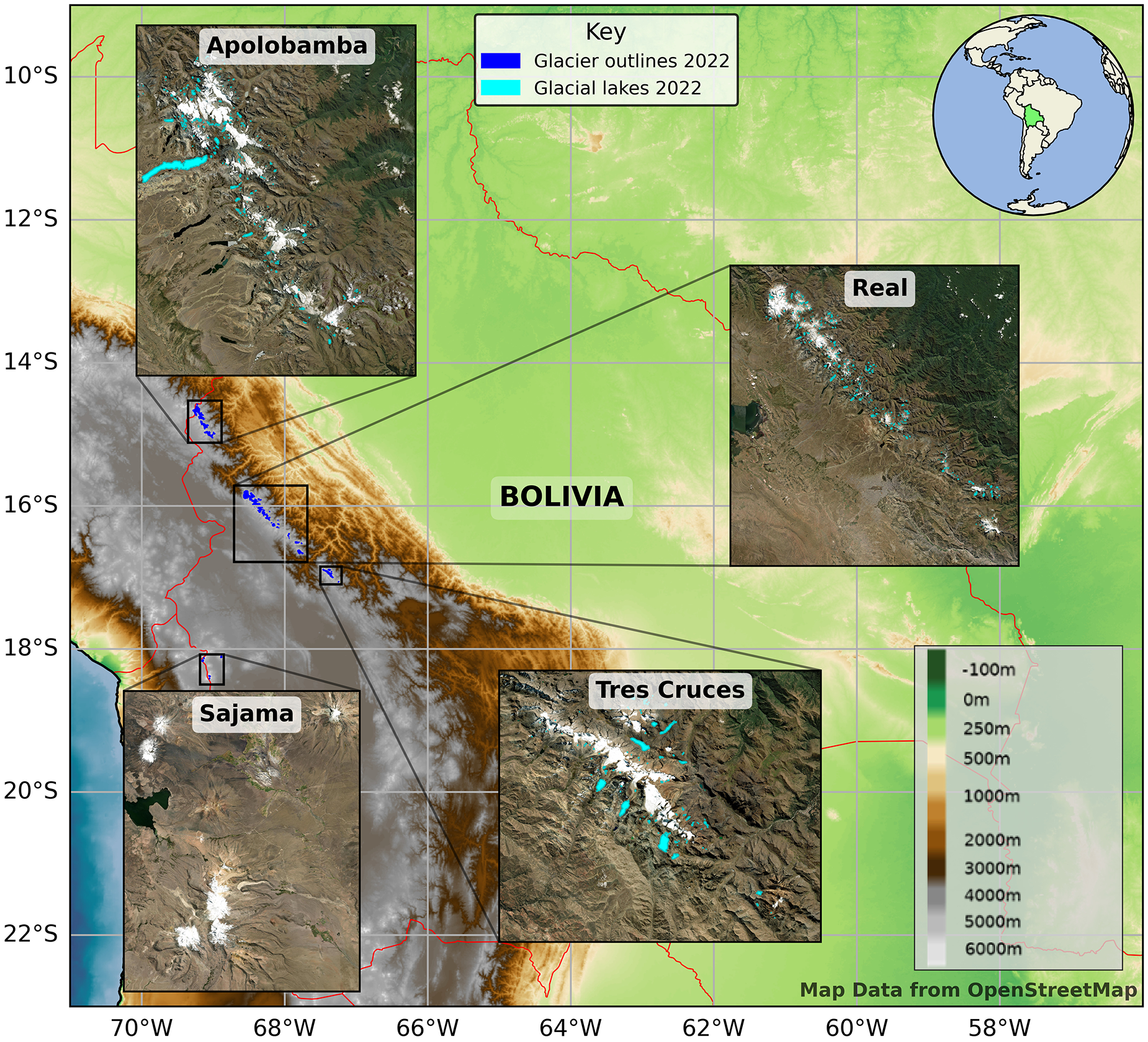
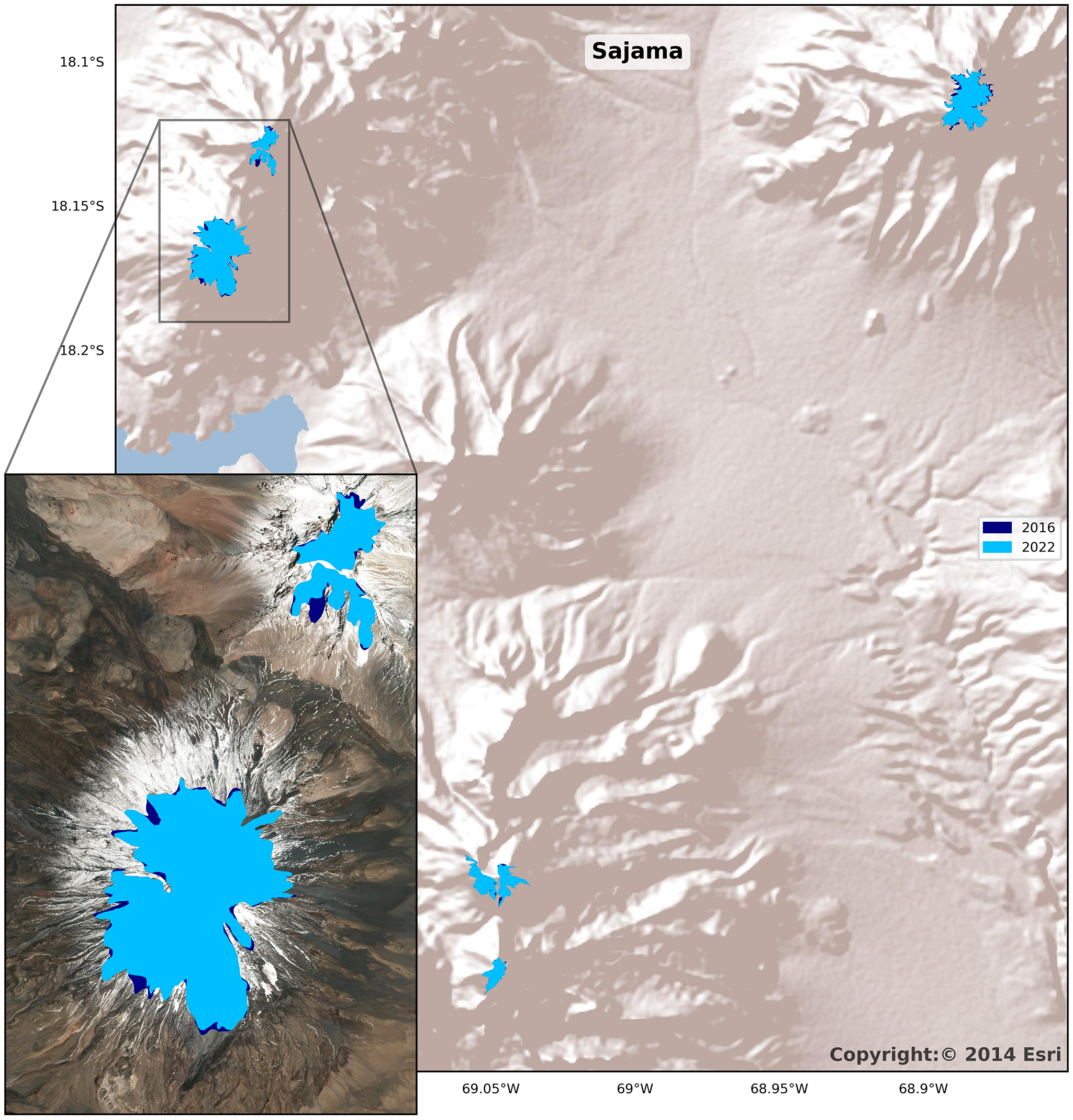
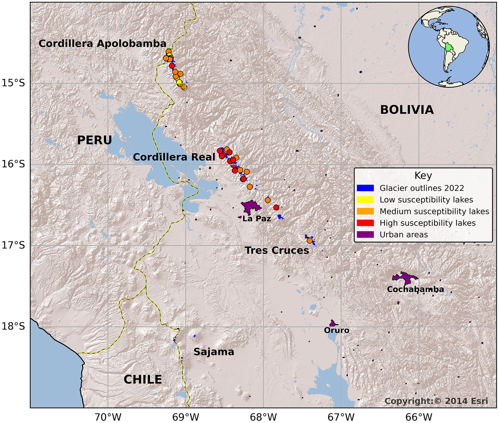
The focus of this study is on the glaciated regions of the Plurinational State of Bolivia (Bolivia; Fig. 1). The southeast third of the country is dominated by the Andes, with several mountain summits above 6000 m. This area contains parts of the Cordilleras Occidental and Central, as well as the Altiplano, which is the second largest high-altitude plateau on Earth. The majority of Bolivia’s ∼420 glaciers are located in the eastern cordillera (Central). These glaciers are distributed across three distinct regions: the Cordilleras Apolobamba, Real, and Tres Cruces. There are also a small number of glaciers in the western cordillera (Occidental) on the flanks of high altitude (∼6000 m) volcanoes in the Sajama region.

Figure 1. Topographic map of Bolivia showing location of glaciers (blue outlines). Inset maps show location of glacial lakes within glaciated regions (Imagery Source: Esri, Maxar, Earthstar Geographics, and the GIS User Community). Inset globe shows location of Bolivia within South America. OpenStreetMap data is available under the Open Database License (https://www.Openstreetmap.Org/copyright).
Quantifying glacier and lake changes between 2016 and 2022
High spatial resolution (3–5 m) orthorectified satellite data were acquired from Planet Labs (Planet Team, 2023). Images were downloaded for each of the areas of interest for each year of the study (2016–2022). Filters were applied to ensure full areal coverage at each time step, with a minimum of cloud cover. Where possible, dry season imagery gathered between May and August was selected to reduce the likelihood of fresh snow obscuring glacier boundaries. For a full list of scenes used, see Supplementary Material Table S1. Glacier outlines were downloaded (as shapefiles) from the Randolph Glacier Inventory (RGI) version 7 database of the Global Land Ice Measurements from Space (GLIMS) initiative (GLIMS, 2023). The Bolivian glacier inventory was compiled from the RGI dataset with reference to the national boundary of Bolivia downloaded from the Humanitarian Data Exchange (HDX) portal of the United Nations Office for the Coordination of Humanitarian Affairs (OCHA) (Humanitarian Data Exchange, 2023). Visual analysis of the subsequent dataset was then undertaken, and the RGI glacier outlines were manually adjusted to the glacier boundaries visible in the Planet imagery for each year of the study period. Polygons with a surface area of less than 0.05 km2 were removed as Bolch and others (Reference Bolch, Menounos and Wheate2010) identify that many features below this size threshold are likely to represent snow patches rather than glaciers. Altitude, slope and aspect data were then extracted for each glacier in the GIS, using the ALOS Global Digital Surface Model (AW3D30). AW3D30 data were obtained from the Japanese Aerospace Exploration Agency (JAXA) (JAXA, 2023). This model was chosen as it is considered to be the most accurate publicly available digital elevation model (DEM), particularly for high mountain regions (Furian and others, Reference Furian, Loibl and Schneider2021).
Initially, lakes were visually identified and digitized from high spatial resolution (3–5 m) Planet data for the year 2022 (Planet Team, 2023). For all other years in the census period, lake boundaries were then manually adjusted with reference to the corresponding Planet satellite data for that year. The altitude of the centroid of each lake was also extracted from the AW3D30 DEM. For the purpose of this study, lakes within 2 km of a glacier boundary were classified as glacial lakes in order for the results to be directly comparable with those of Cook and others (Reference Cook, Kougkoulos, Edwards, Dortch and Hoffmann2016). Uncertainty in mapping both glaciers and lakes was estimated using the method described by Hanshaw and Bookhagen (Reference Hanshaw and Bookhagen2014), as shown in Equation 1. They assumed that area measurement error is normally (i.e. Gaussian) distributed. The total perimeter ( $P$) of mapped features was therefore divided by grid-cell size ( $G$—the largest spatial resolution of images used). This number was multiplied by 0.6872 ( $1\sigma $) as it was assumed that ∼69% of pixels contain errors. Finally, it was assumed that the uncertainty for each pixel is half a pixel, so the resulting number was multiplied by half of the area of a single pixel.
 \begin{equation}Error{ }\left( {1\sigma } \right) = \left( {\frac{P}{G}} \right){ } \times 0.6872{ } \times \left( {\frac{{{G^2}}}{2}} \right)\end{equation}
Using this method, mapping uncertainties are estimated at ∼1% for glaciers and ∼2% for glacial lakes.
Assessing GLOF susceptibility from the 2022 glacial lake inventory
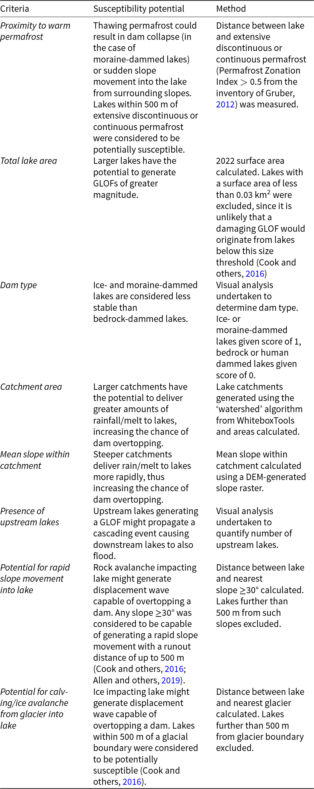
We developed a susceptibility assessment protocol for GLOFs from the mapped lakes in Bolivia. The starting point for this was the Glacial and Permafrost Hazards in Mountains (GAPHAZ) Technical Document, which identifies 25 factors that contribute to a lake’s susceptibility to GLOF generation (henceforth GLOF susceptibility) (GAPHAZ, Reference GAPHAZ2017). Of these, the GAPHAZ guidelines indicate that 13 factors are best suited to analysis at the basin or site-specific level. These factors were, therefore, excluded because the aim of the present study is to quantify susceptibility at a regional level. Of the remaining 12 factors, seismicity and lake growth were excluded as it was assumed that there is no significant variation in seismicity across the study area, and recent research has questioned the role of both in triggering GLOFs (Fischer and others, Reference Fischer, Korup, Veh and Walz2021; Wood and others, Reference Wood2024; Veh and others, Reference Veh2025). Four of the remaining factors were linked to rainfall/snowmelt, but this trigger is rather rare in the Bolivian Andes (Emmer and others, Reference Emmer2022), and so stream order and drainage density were also excluded. The derived inventory of lakes in 2022 was therefore assessed for GLOF susceptibility against a set of eight criteria (Table 1). This study focused on a lake’s susceptibility to GLOF generation rather than the potential threat posed to people or infrastructure in the event of a GLOF taking place (risk; e.g. Kougkoulos and others, Reference Kougkoulos2018a, b).
Table 1. Criteria used in ascertaining GLOF susceptibility of glacial lakes in 2022 lake inventory.

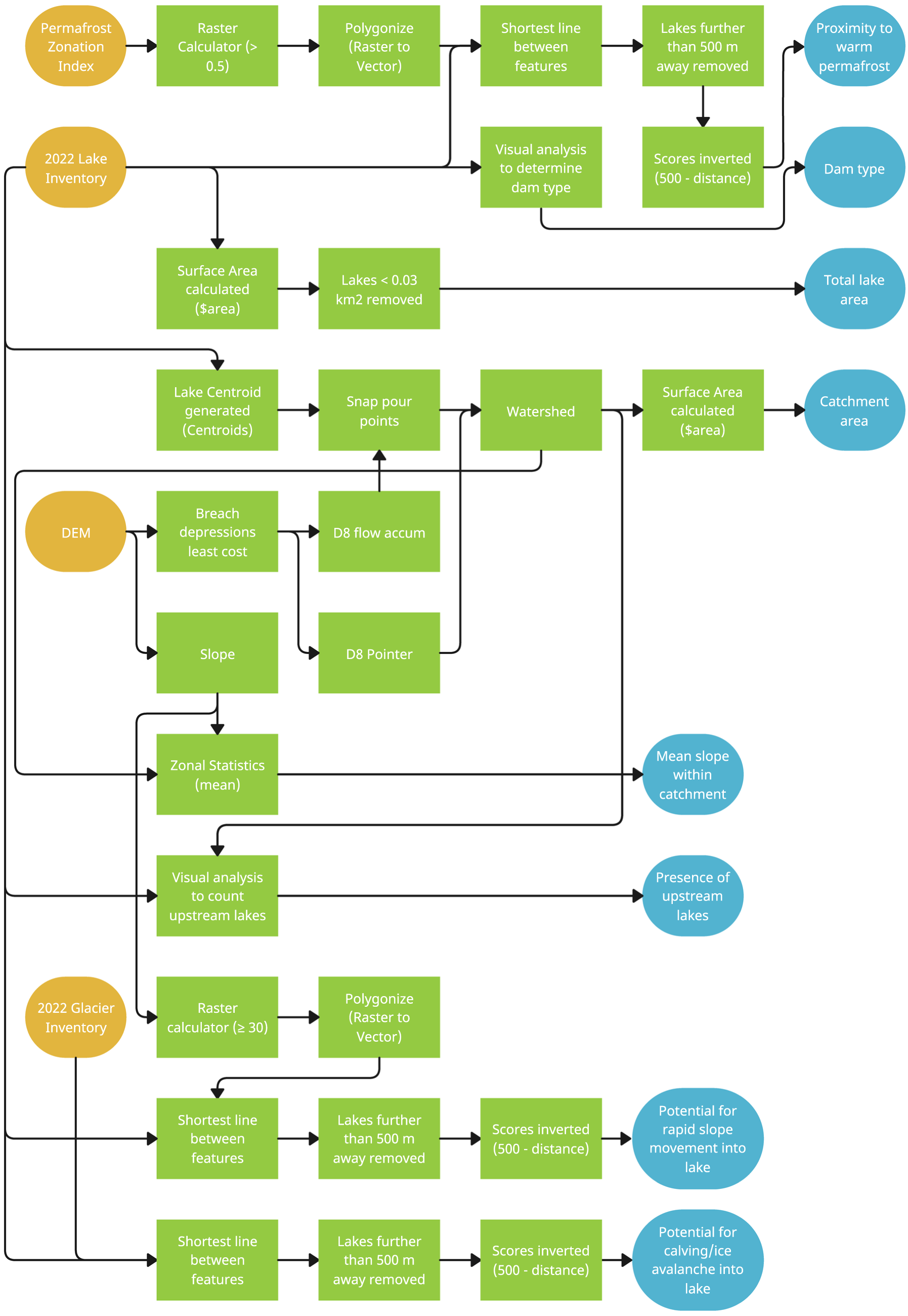
All geospatial analysis was undertaken in QGIS 3.22.11 (Białowieża). Hydrological analysis was performed using the WhiteboxTools plugin from Whitebox Geospatial (Whitebox Geospatial Inc, 2023). An individual susceptibility score for each of the eight criteria identified in Table 1 was generated for each lake using the workflow outlined in Fig. 2. All individual susceptibility scores were then normalized to between 0 and 1 using Equation 2:
 \begin{equation}z_i = \left( {{x_i} - \min \left( x \right)} \right)/\left( {\max \left( x \right) - \min \left( x \right)} \right)\end{equation}
Figure 2. GIS workflow showing input layers (Orange polygons), processes (green rectangles) and output susceptibility scores (blue polygons). Susceptibility scores were then normalized and summed to give an overall susceptibility rating according to Equation 2.
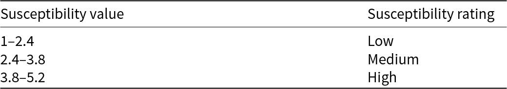
where zi is the ith normalized value in the dataset and xi is the ith value in the dataset. Min(x) and max(x) refer to the minimum and maximum values in the dataset. Normalized susceptibility scores were then summed to give an overall susceptibility value out of eight for each lake. All susceptibility scores were given an equal weighting. A susceptibility rating of ‘low’, ‘medium’ or ‘high’ was then assigned to each lake based on an equal interval classification of the calculated susceptibility values (Table 2).
Table 2. Susceptibility rating derived from calculated susceptibility values.

Analysis of subglacial topography to identify potential sites for future lake formation
The global consensus glacier ice thickness database of Farinotti and others (Reference Farinotti2019a) was analysed to identify subglacial overdeepenings that represent potential sites for future lake formation. Farinotti and others (Reference Farinotti2019a) applied the models of Huss and Farinotti (Reference Huss and Farinotti2012), Frey and others (Reference Frey2014), and Maussion and others (Reference Maussion2018) to the void-filled Shuttle Radar Topography Mission (SRTM) DEM version 4 to generate their consensus ice thickness dataset for Bolivia. SRTM DEM data were acquired in February, 2000. Surface topography and glacier ice thickness datasets were downloaded from the ETH Zürich Research Collection (Farinotti and others, Reference Farinotti2019b). Initially, a ‘DEM without glaciers’ was produced by subtracting glacier ice thickness from surface topography. The resulting DEM was filled using the ‘Fill Depressions’ algorithm from Whitebox Geospatial (Whitebox Geospatial Inc, 2023) in QGIS 3.22.11 (Białowieża). Subtracting the DEM without glaciers from the filled DEM yielded a raster layer where pixels with a non-zero value represented sites of subglacial overdeepenings. In addition, this process yielded an estimate of their bathymetry, allowing depth, surface area, and volume to be calculated.
Furian and others (Reference Furian, Loibl and Schneider2021) suggest that overdeepenings below a certain size threshold are more likely to fill up with sediment than with water. Based on previous work (e.g. Linsbauer and others Reference Linsbauer, Frey, Haeberli, Machguth, Azam and Allen2016; Colonia and others, Reference Colonia2017), they identified a threshold surface area of 0.1 km2 and a depth of 5 m for their study of subglacial overdeepenings in High Mountain Asia. However, Cook and others (Reference Cook, Kougkoulos, Edwards, Dortch and Hoffmann2016) cite the example of a damaging GLOF in 2009, which affected the village of Keara in Bolivia (Hoffmann and Weggenmann, Reference Hoffmann and Weggenmann2013). They highlighted that the lake which generated the flood was relatively small (0.034 km2) and proposed a size threshold of 0.03 km2 for potentially hazardous lakes in Bolivia. Given that future lakes capable of producing damaging GLOFs are of primary interest, we chose to apply the lower surface area threshold of 0.03 km2 and the depth threshold of 5 m.
The resulting dataset was then manually validated to remove unrealistic overdeepenings caused by erroneous void filling, by comparison with the Planet imagery. Ensemble model uncertainty for the region is calculated as ±30% (Farinotti and others, Reference Farinotti2019a) and so a corresponding uncertainty is assumed here for calculations of depth, surface area, and volume. The global glacier thickness dataset of Farinotti and others (Reference Farinotti2019a) relies on glacier outlines from the RGI version 6.0 (GLIMS, 2017). In Bolivia, these outlines are derived from imagery from the year 2000. As a result of glacial recession between 2000 and 2022, there is an opportunity to test modelled lake locations against those which have appeared in the region during this time period.
Results
Glacier change between 2016 and 2022
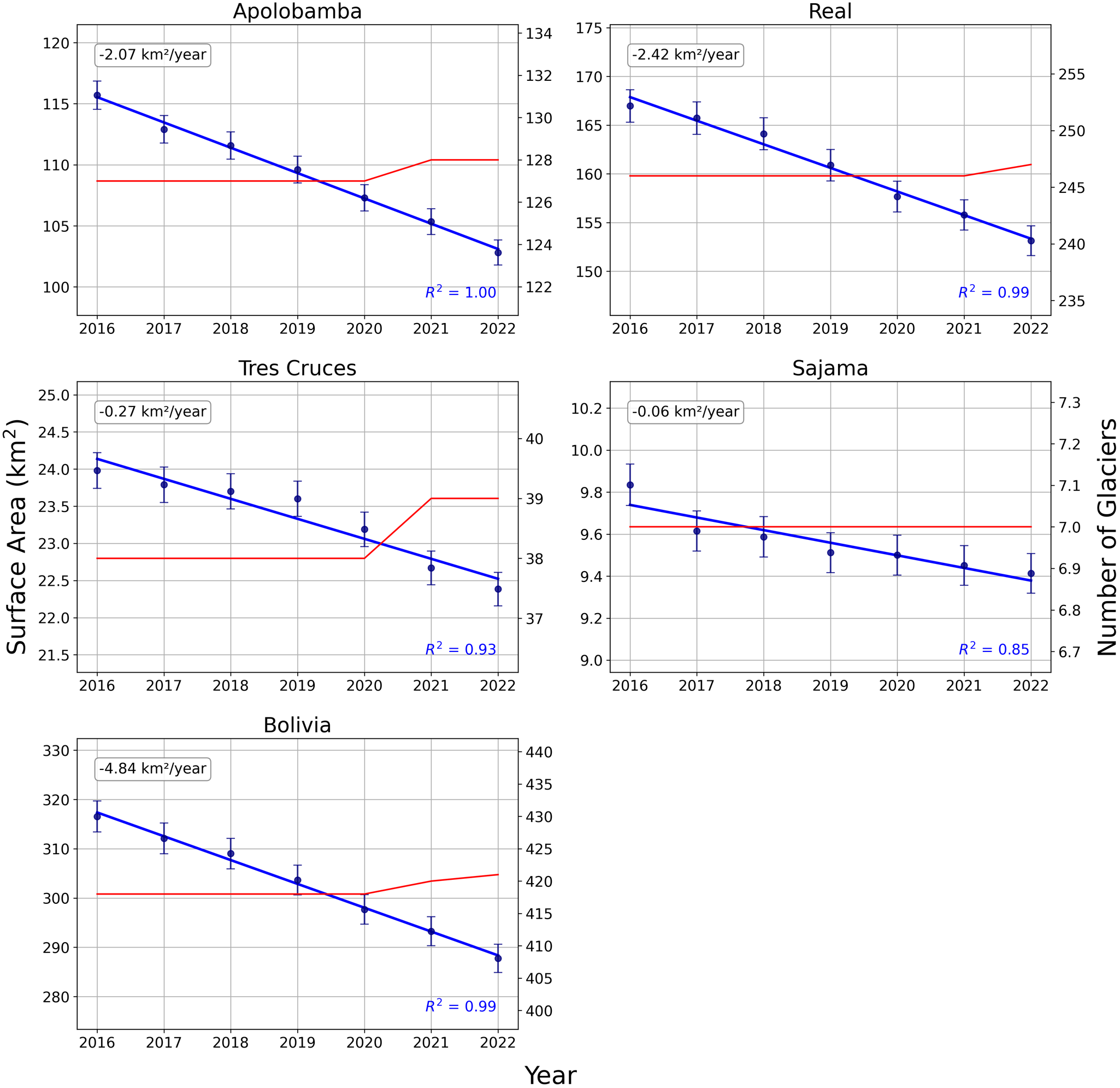
The total glacier-covered area of the Bolivian Andes decreased by 9.1%, from 316.6 ± 3.2 km2 in 2016 to 287.8 ± 2.9 km2 in 2022, representing a rate of ice loss of 4.8 km2 a−1 (Fig. 3). The largest loss was from the Cordillera Real (13.8 km2) and the smallest from the Sajama region (0.4 km2), although all four areas were subject to a reduction in ice cover over the study period (Figs. 4–7). In 2022, the majority of Bolivian glaciers had a surface area of less than 1 km2, occupied a median altitude of between 5200 and 5400 masl, with an average slope of between 15 and 35°, and faced in a southerly direction (Supplementary Material Fig. S1).

Figure 3. Total surface area (navy blue points) and number of glaciers (red lines) in each region by year. Navy blue bars represent mapping uncertainty. Note different scales on y-axes.

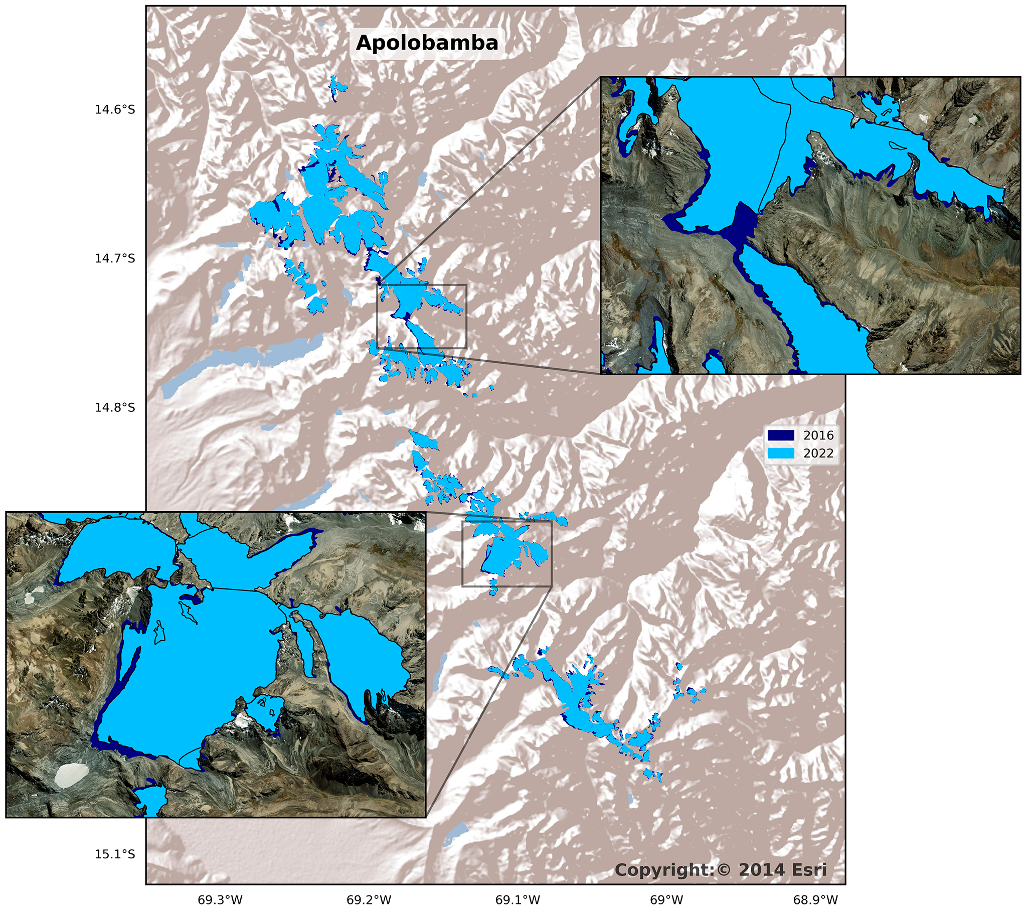
Figure 4. Change in glacier surface area between 2016 (dark blue) and 2022 (light blue) in the Cordillera Apolobamba. Insets show detail in selected regions. Imagery Source: Esri, Maxar, Earthstar Geographics, and the GIS User Community.

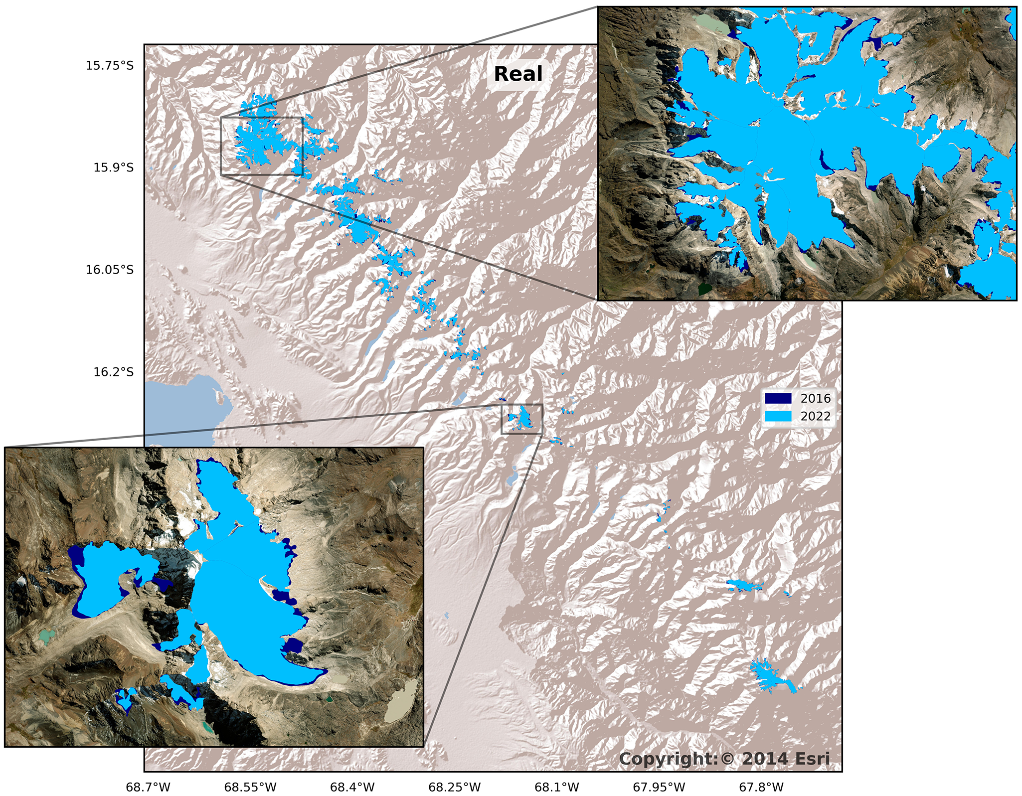
Figure 5. Change in glacier surface area between 2016 (dark blue) and 2022 (light blue) in the Cordillera Real. Insets show detail in selected regions. Imagery Source: Esri, Maxar, Earthstar Geographics, and the GIS User Community.

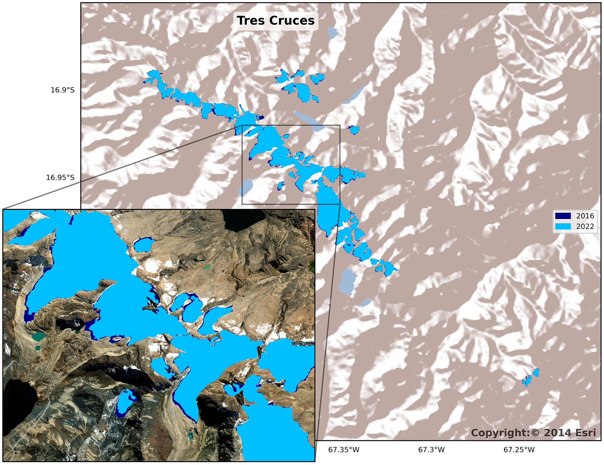
Figure 6. Change in glacier surface area between 2016 (dark blue) and 2022 (light blue) in Tres Cruces. Inset shows detail in selected region. Imagery Source: Esri, Maxar, Earthstar Geographics, and the GIS User Community.

Figure 7. Change in glacier surface area between 2016 (dark blue) and 2022 (light blue) in Sajama. Inset shows detail in selected region. Imagery Source: Esri, Maxar, Earthstar Geographics, and the GIS User Community.
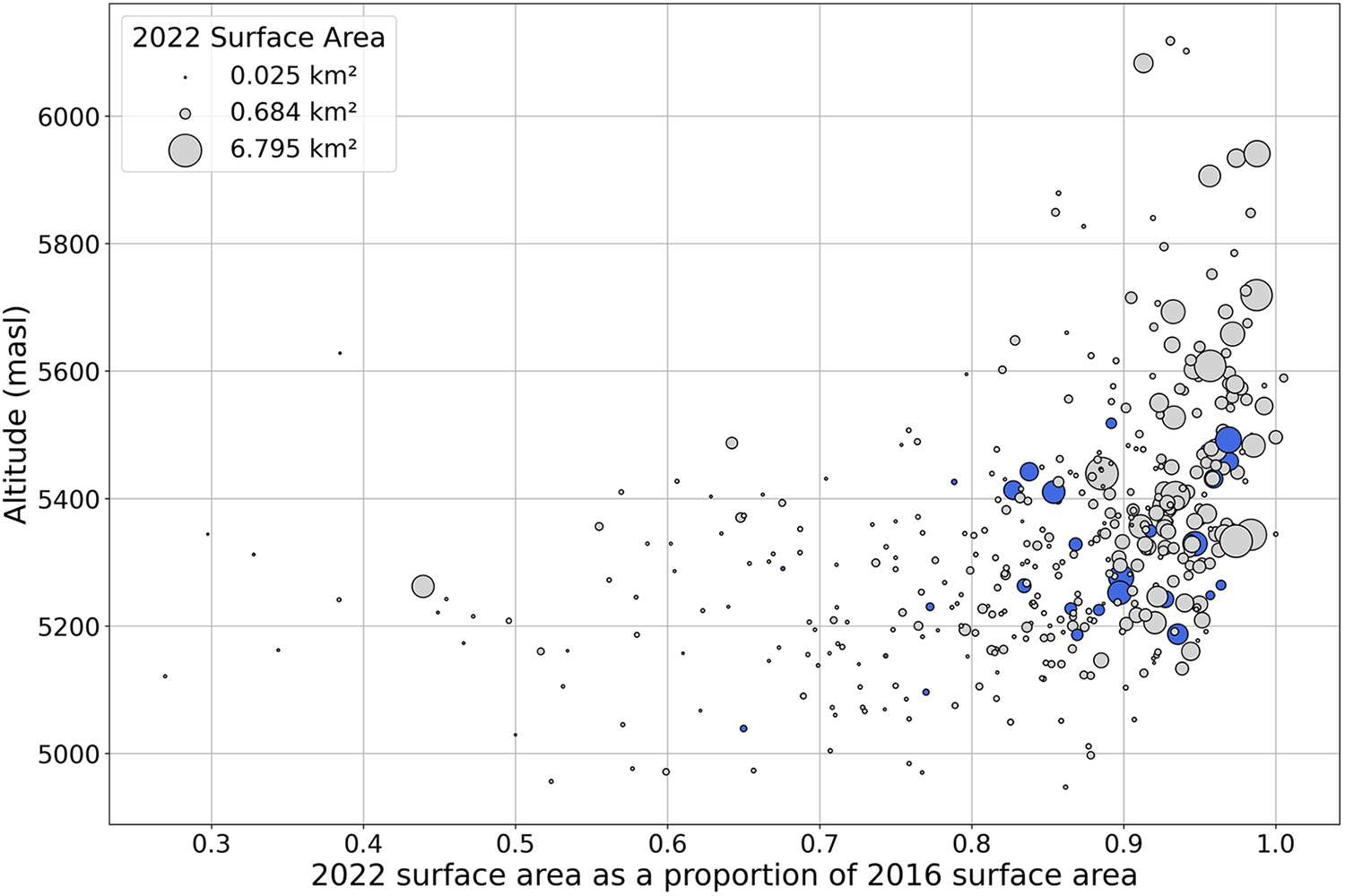
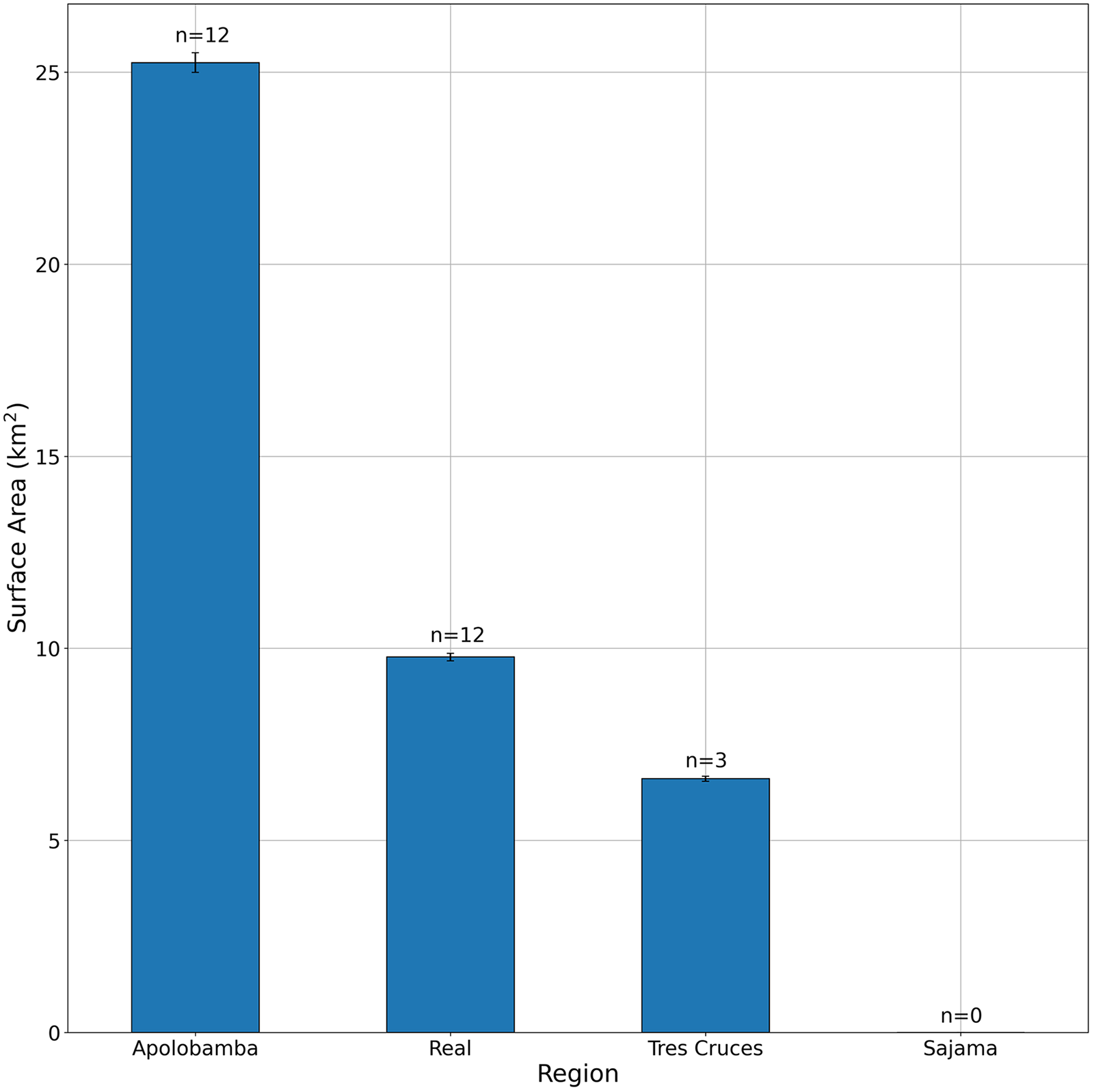
Larger glaciers, and those at higher elevations, tended to lose a lesser proportion of their surface area than smaller glaciers, and those at lower elevations (Fig. 8). The number of lake-terminating glaciers increased by 42%, from 19 in 2016 to 27 in 2022 (Supplementary Material, Fig. S2). The total surface area of lake-terminating glaciers was 41.63 ± 0.42 km2 in 2022. More than half of this surface area was in the Cordillera Apolobamba (Fig. 9). There did not appear to be any correlation between the proportion of surface area lost by a glacier and whether it terminated on land or in a glacial lake (Fig. 8).

Figure 8. Change in glacier surface area by altitude. Size of points is relative to size of glacier. Lake terminating glaciers are represented by blue points.

Figure 9. Surface area of lake terminating glaciers by region. Black bars represent mapping uncertainty.
Glacial lake change between 2016 and 2022
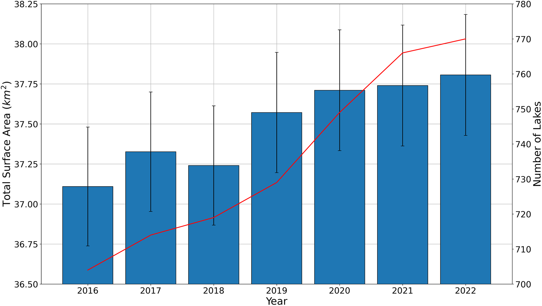
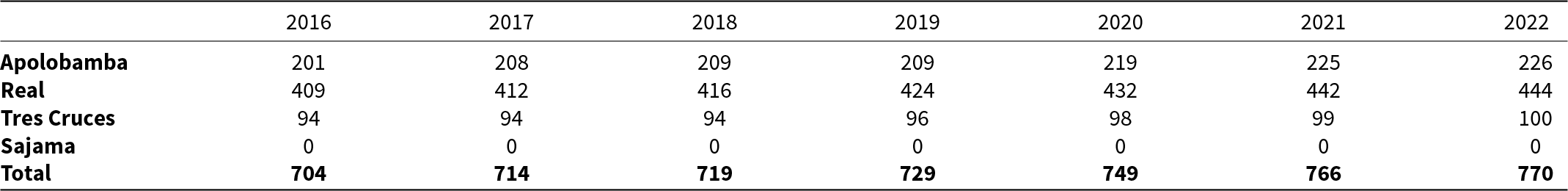
In 2022, there were 770 glacial lakes within 2 km of a glacier boundary (Table 3). This represented a 2.6% increase in the number of lakes since 2016. 57.7% of these lakes were located in the Cordillera Real, whilst the Sajama region contained no glacial lakes. The total surface area of glacial lakes increased by 1.9%, from 37.1 ± 0.7 km2 in 2016 to 37.8 ± 0.8 km2 in 2022 (Fig. 10).

Figure 10. Surface area (blue bars) and number of lakes (red line) by year. Black bars represent mapping uncertainty. Note that neither y-axis starts at 0.
Table 3. Distribution of glacial lakes across the Bolivian Andes.

GLOF susceptibility potential of 2022 glacial lake inventory
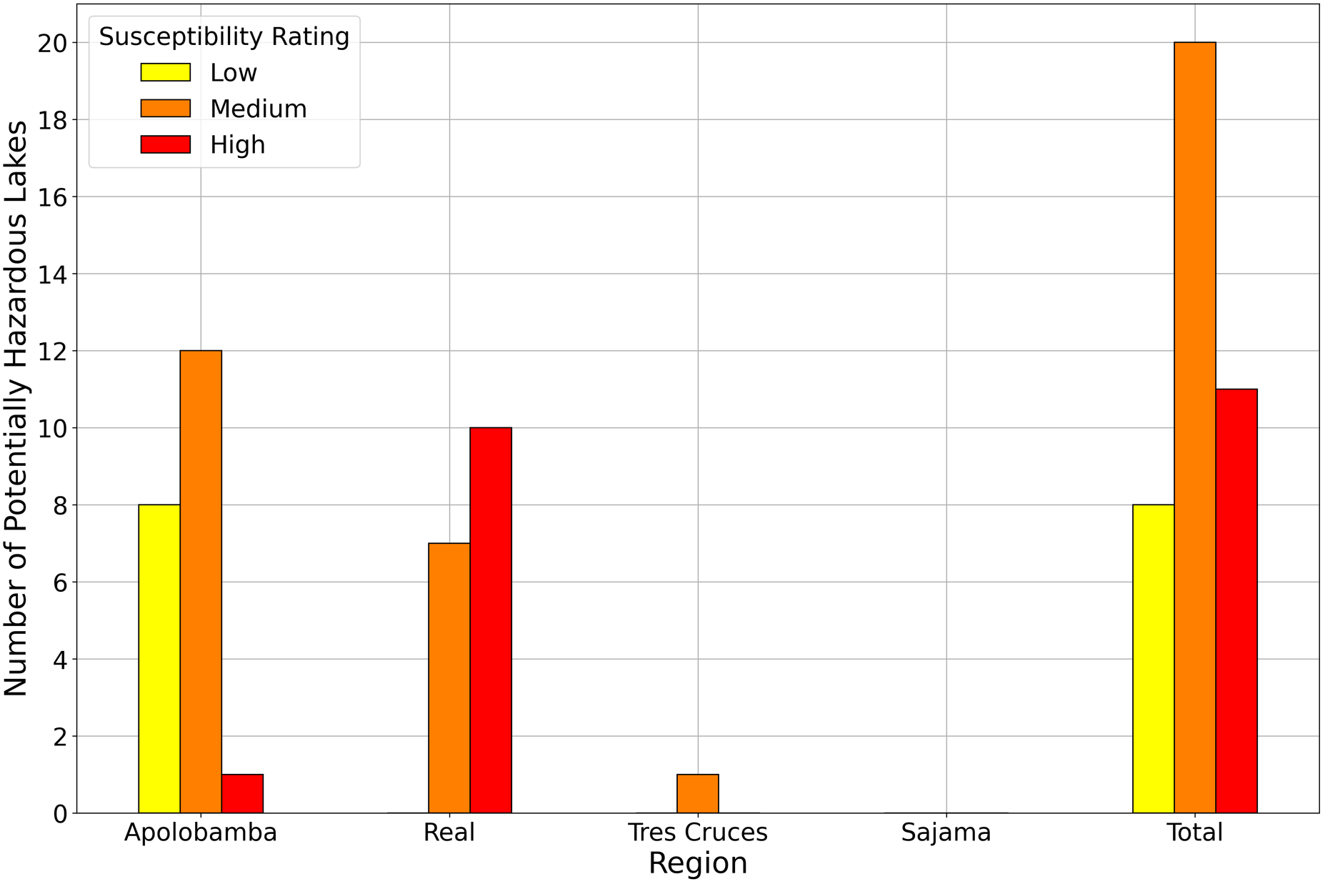
Of the 770 lakes identified in the 2022 inventory, 120 had a surface area ≥ the size threshold of 0.03 km2; 39 of these lakes were located within 500 m of both a glacier boundary and a slope ≥ 30°. Following the susceptibility analysis, 8 (21%) of these were categorized as ‘low susceptibility’, 20 (51%) as ‘medium susceptibility’ and 11 (28%) as ‘high susceptibility’ (Supplementary Material, Table S2). The locations of these potentially susceptible lakes are shown in Fig. 11. The majority of lakes designated potentially susceptible are located in the Cordillera Apolobamba (n = 21), but most lakes with a high susceptibility rating are located in the Cordillera Real (n = 10) (Fig. 12).

Figure 11. Location and susceptibility rating of potentially susceptible lakes across the Bolivian Andes. Urban areas were downloaded from the Center For International Earth Science Information Network (CIESIN) – Columbia University and Joint Research Centre (JRC) – European Commission (2024).

Figure 12. Number and susceptibility rating of potentially susceptible lakes in each region.
Potential sites for future lake formation
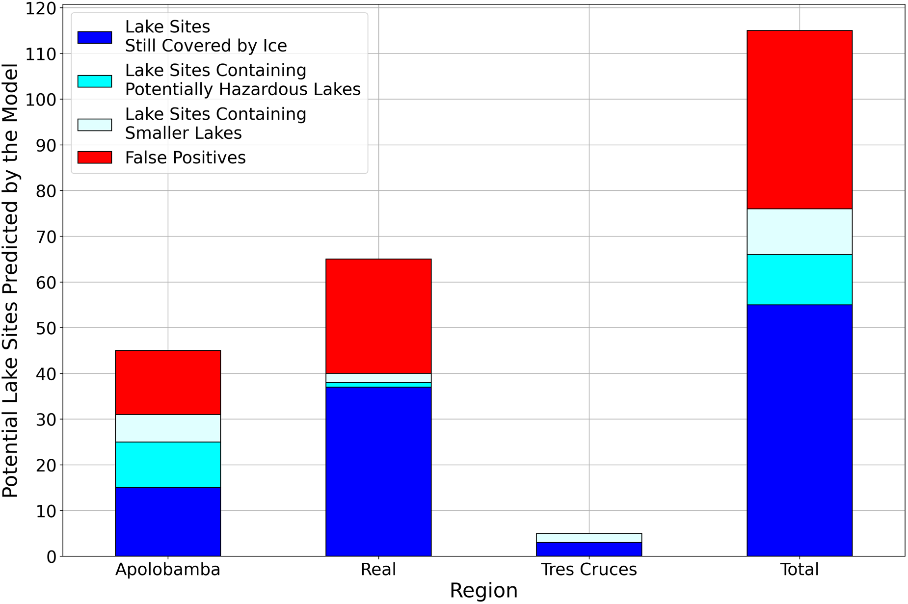
In total, the model identified 115 potential lake sites across all glacierized regions of Bolivia, except for Sajama (Fig. 13, Supplementary Material, Fig. S4). Sixty-five (57%) of these sites are in the Cordillera Real (Fig. 14). Of the 115 potential sites identified, 60 are located in areas which deglaciated between 2000 and 2022 (Fig. 13). Eleven of these hosted potentially susceptible lakes in 2022, with an additional 10 sites containing smaller lakes. A further 39 sites (65%) therefore represent false positives. A total of 22 potentially susceptible lakes formed between 2000 and 2022, 14 of which occupied overdeepenings predicted by the model. The other 8 lakes therefore represent false negatives (Supplementary Material, Fig. S5).

Figure 13. Potential lake sites identified by the model in each region. No sites were located in Sajama.

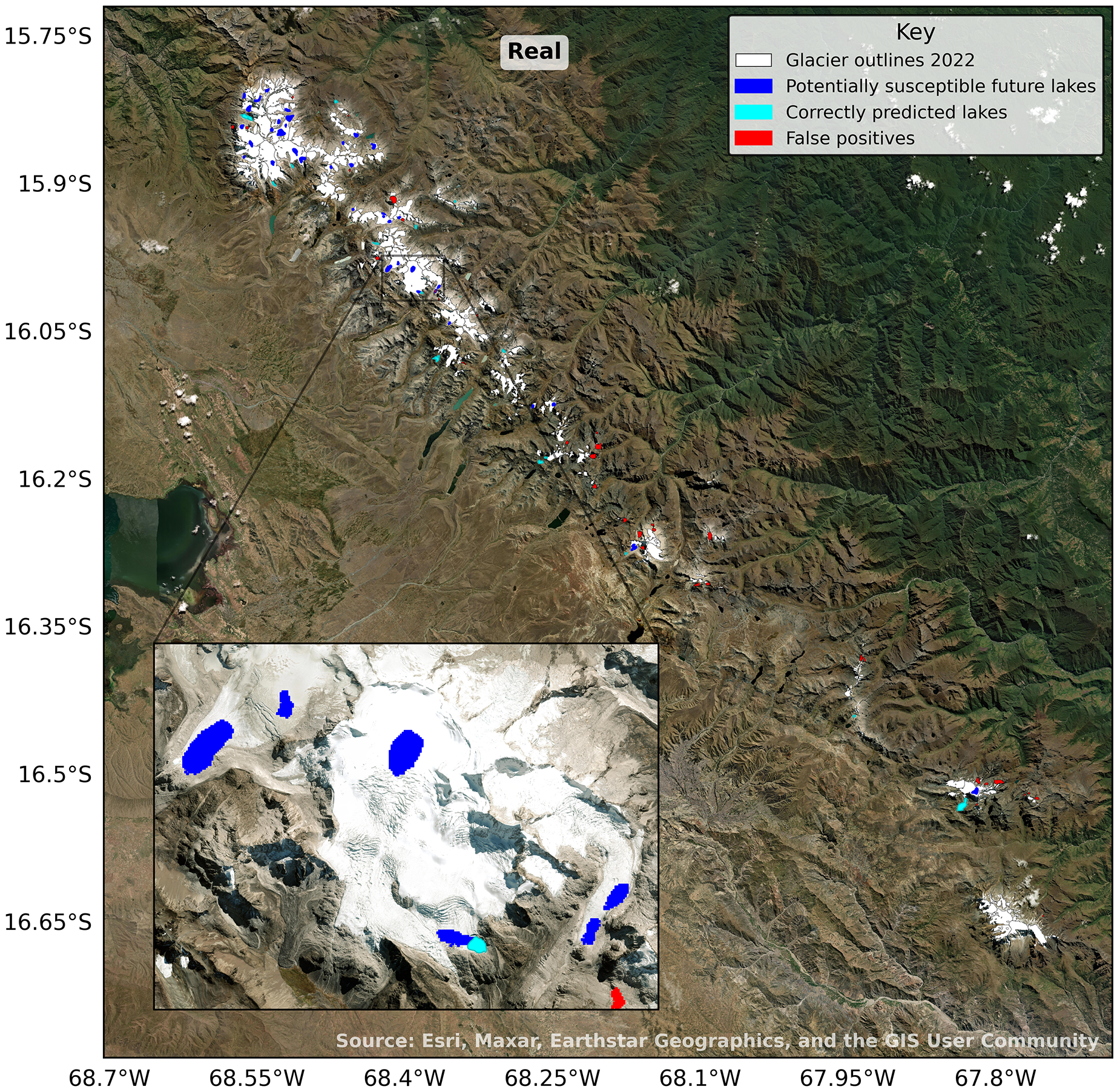
Figure 14. Modelled lakes in the Cordillera Real. Blue lakes are those predicted to form given continued glacier recession, whilst cyan lakes are those correctly predicted by the model to form between 2000 and 2022. Red lakes are those predicted by the model which did not form. Inset map shows detail for clarity. For a map of all modelled lake locations, see Supplementary Material, Figure S4.
Should lakes form at all of the potential sites still covered by ice, the total surface area (volume) of these lakes is projected to be ∼6.4 km2 (∼5.7 million cubic metres) (Table 4). Of these potential future lakes, only one is predicted to have a surface area greater than 0.4 km2, with most being smaller than 0.2 km2 (Supplementary Material, Fig. S3). The lakes are projected to form between 4900 and 5900 masl and range in depth (volume) from ∼10 to ∼200 m (∼0.003 to ∼0.67 million cubic metres).
Table 4. Projected future lake sites by region.

Discussion
Glacier change
Change in glacier surface area
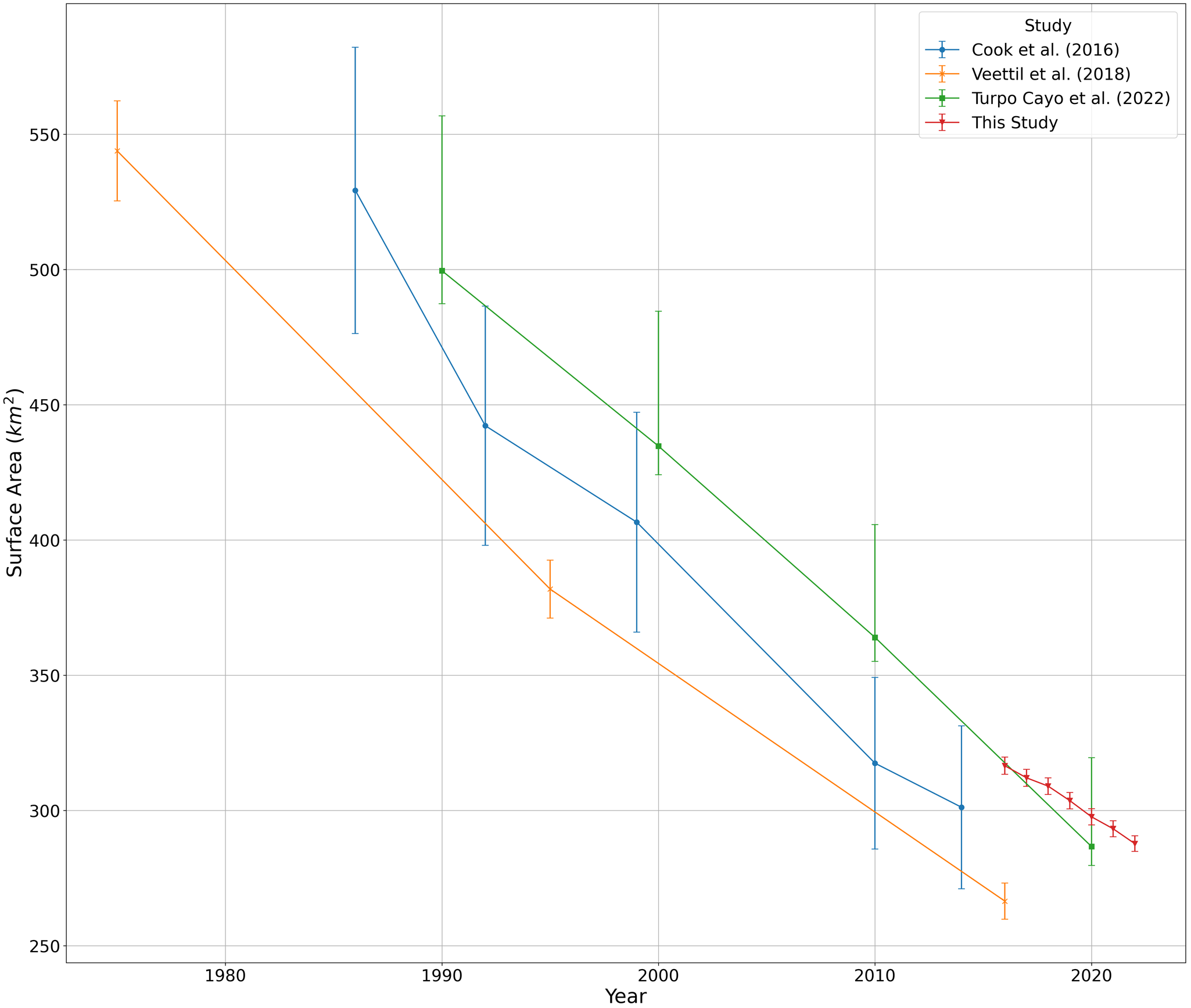
During the study period, the total glacier-covered area of the Bolivian Andes reduced by 28.8 ± 0.3 km2, from 316.6 ± 3.2 km2 in 2016 to 287.8 ± 2.9 km2 in 2022 (Fig. 3). This represents a decrease of 9.1% over six years. The results of previously published glacier inventories for Bolivia are shown in Table 5. Our results are broadly consistent with these previous studies once methodological and spatial coverage factors are taken into account. Cook and others (Reference Cook, Kougkoulos, Edwards, Dortch and Hoffmann2016) reported a total surface area in 2014 that was ∼15 km2 lower than that found by this study for 2016. Given the consistent reporting of glacier recession in this region, it is unlikely that this discrepancy represents glacier growth during this 2-year period (Veettil and Kamp, Reference Veettil and Kamp2017; Vuille and others, Reference Vuille2018; Gorin and others, Reference Gorin2024). A substantial contributor to this discrepancy is that Cook and others (Reference Cook, Kougkoulos, Edwards, Dortch and Hoffmann2016) inventory did not include glaciers in the Sajama region, which accounted for an area of 9.84 ± 0.1 km2 in 2016. Another possible contributor to this discrepancy is the use of finer spatial resolution (3–5 m pixel resolution) Planet satellite imagery in this study compared to the coarser resolution Landsat data used by Cook and others (Reference Cook, Kougkoulos, Edwards, Dortch and Hoffmann2016) (30 m per pixel). In any case, the 2016 figure presented here falls comfortably within the margin for error calculated by Cook and others (Reference Cook, Kougkoulos, Edwards, Dortch and Hoffmann2016) (Fig. 15).

Figure 15. Comparison of rates of loss between that found by this study and those in previously published work.
Table 5. Comparison of total glacier-covered area found by this and previous studies.

A larger discrepancy exists between the results of this study and those reported by Veettil and others (Reference Veettil, Wang, Simões and Pereira2018). They also excluded glaciers in the Sajama region from their study, which goes some way to explaining the disagreement between the two sets of results. Furthermore, it is unclear whether glaciers that overlap the border between Peru and Bolivia were included in or excluded from their study, which could also be a substantial contributor to apparent discrepancies. Another possible contributor is the difference in methodology between the two studies. Veettil and others (Reference Veettil, Wang, Simões and Pereira2018) utilized an automated approach, which can be affected by misidentification of snow as glacier ice, and relied upon coarser Landsat and Sentinel-2 imagery. Turpo Cayo and others (Reference Turpo Cayo2022) found a lower value for glacier cover in 2020, but their study acknowledged omission errors (i.e. where glaciers will not have been mapped) of 11.46%, with the greatest errors found during the first (1985) and last (2020) years of their study period. They highlight that shaded areas and small glaciers were the source of most omission errors. Given that ∼75% of Bolivian glaciers had a surface area less than 1 km2 in 2022 (Supplementary Material, Fig. S1), it may be that the glacier-covered area in 2020 was greater than they reported, and overall the findings of this study are comfortably within their reported margins of error (Fig. 15).
Rate of glacier surface area change
The glacier-covered area of the Bolivian Andes diminished at a rate of 4.8 km2 a−1 between 2016 and 2022. This rate of surface area loss is congruent with those found by Cook and others (Reference Cook, Kougkoulos, Edwards, Dortch and Hoffmann2016) and Veettil and others (Reference Veettil, Wang, Simões and Pereira2018) for the periods between 2010 and 2014 (4.0 km2 a−1) and 1995 to 2016 (5.5 km2 a−1), respectively. It is, however, lower than that identified by Turpo Cayo and others (Reference Turpo Cayo2022) for the period 2010 to 2020 (7.7 km2 a−1) (Fig. 15). Given the broad agreement between the results of this study and the studies of Cook and others (Reference Cook, Kougkoulos, Edwards, Dortch and Hoffmann2016) and Veettil and others (Reference Veettil, Wang, Simões and Pereira2018), it is possible that the accelerated rate of loss identified by Turpo Cayo and others (Reference Turpo Cayo2022) might be attributable to an anomalously low surface area for their 2020 glacier inventory, as discussed in the previous section.
Drivers of surface area change
The sustained reduction in the glacier-covered area of the Bolivian Andes has been attributed to rising temperatures associated with climate change (Rabatel and others, Reference Rabatel2013; Rangecroft and others, Reference Rangecroft, Harrison, Anderson, Magrath, Castel and Pacheco2013). The ongoing warming trend evident across the Tropical Andes in previous decades has resulted in the raising of the 0°C isotherm, and a concomitant rise in the equilibrium line altitude (ELA)—where glacier accumulation is equal to ablation (Rangecroft and others, Reference Rangecroft, Harrison, Anderson, Magrath, Castel and Pacheco2013). Thus, glaciers are subject to enhanced ablation and reduced accumulation, resulting in negative mass balances. Rabatel and others (Reference Rabatel2013) also identified that glacier mass balance amongst tropical Andean glaciers is strongly associated with sea surface temperature (SST) anomalies in the Pacific Ocean. They assert that positive (negative) ENSO phases closely correspond to periods of suppressed (enhanced) melt, with response times typically in the order of four months for glaciers in the outer tropics. They highlight that negative ENSO phases (El Niño conditions) result in a decrease in precipitation of 10–30%, more frequent dry periods during austral summer, and near-surface temperatures 0.7–1.3 °C warmer than during positive phases (La Niña conditions). These conditions result in increased insolation, reduced snow accumulation, decreased albedo, and increased sensible heat flux at the glacier surface (Rabatel and others, Reference Rabatel2013). Given that strongly positive ENSO phases dominated for all but one year of the study period (NCEI, 2023), it appears likely that the observed rate of change was lower than it would otherwise have been.
Local factors specific to individual glaciers also play an important role in mass balance. Between 2016 and 2022, larger glaciers and those at higher elevations lost a lesser proportion of their surface area than smaller glaciers and those at lower elevations (Fig. 8). This continues a trend identified by previous studies in the region (e.g. Veettil and others, Reference Veettil, Wang, de Souza, Bremer and Simões2017; Turpo Cayo and others, Reference Turpo Cayo2022). This has been explained by Vuille and others (Reference Vuille2008) as an ‘edge effect’ whereby smaller glaciers become more vulnerable to mass loss by warm air advection from adjacent rock surfaces that warm in daylight. Furthermore, as the glacier ELA rises with warming temperatures, glaciers at lower altitudes are left without an accumulation zone (Vuille and others, Reference Vuille2008; Richardson and others, Reference Richardson, Carr and Cook2024). In addition, glaciers at lower altitudes are increasingly likely to be exposed to liquid precipitation during the wet season (Veettil and others, Reference Veettil, Wang, Simões and Pereira2018). This has the dual impact of reducing the potential for accumulation and decreasing the albedo of the glacier’s surface. Given that the majority of Bolivian glaciers have a surface area of less than 1 km2 and a median altitude of less than 5400 m a.s.l. (the ELA of Bolivian glaciers is ∼5800 m a.s.l.; Braun and others, Reference Braun2019), it appears that the Bolivian glacier population is particularly vulnerable to continued warming.
Glacier recession is known from several studies to be accelerated by the development of glacial lakes as glaciers are able to lose mass via calving in addition to melting and sublimation (King and others, Reference King, Bhattacharya, Bhambri and Bolch2019; Sutherland and others, Reference Sutherland, Carrivick, Gandy, Shulmeister, Quincey and Cornford2020; Zhang and others, Reference Zhang2023; Scoffield and others, Reference Scoffield, Rowan, Quincey, Carrivick, Sole and Cook2024). However, our results indicate that there is no difference in glacier surface area change between lake- and land-terminating glaciers (Fig. 8). It is possible that this is a function of the relatively short timescale of our study where other factors may have had a more dominant role. Another explanation might be that lake-terminating glaciers in Bolivia did experience enhanced mass loss, but via thinning and speed-up (Li and others, Reference Li, Ding, Shangguan and Wang2019) where we only assessed surface area loss. It is also possible that the extant glacial lakes in Bolivia are unusually shallow for their surface area, and so the influence of the lake on calving rate is limited (Brown and others, Reference Brown, Meier and Post1982; Benn and others, Reference Benn, Warren and Mottram2007). Collectively, there is little known about glacial lake bathymetry, glacier velocity and ice thinning rates in the Bolivian Andes; all of these factors warrant further investigation.
Glacial lake changes 2016–2022
Both the number and surface area of glacial lakes in Bolivia increased over the course of the study period, in keeping with the global trend highlighted by Shugar and others (Reference Shugar2020) (Fig. 10). This followed an overall increase in lake number and size between 1986 and 2014 reported by Cook and others (Reference Cook, Kougkoulos, Edwards, Dortch and Hoffmann2016). They found a total of 225 lakes (with a surface area of 8.73 ± 0.87 km2) within ∼2 km of a glacial boundary in 2014. This contrasts with the 704 lakes (with a surface area of 37.1 ± 0.7 km2) identified in 2016. The large disparity between the two datasets is likely attributable to the higher resolution (3–5 m) Planet imagery available to this study, in comparison to the (30 m resolution) Landsat imagery employed by Cook and others (Reference Cook, Kougkoulos, Edwards, Dortch and Hoffmann2016). The order of magnitude greater resolution facilitated identification of smaller lakes, particularly those close to glacier margins. Such lakes can be difficult to discern given the similar reflectance properties of lakes and glacier ice.
GLOF susceptibility analysis
Cook and others (Reference Cook, Kougkoulos, Edwards, Dortch and Hoffmann2016) identified 25 lakes in 2014 that had the potential to produce damaging GLOFs (Table 6). All but four of these lakes were still considered to be potentially susceptible in 2022. Of the four that were not considered to remain a threat, three were no longer within 500 m of a glacier margin, whilst the fourth had a surface area less than the 0.03 km2 size threshold. A further 18 lakes were designated as potentially susceptible by this study. Some of these lakes did not exist when Cook and others (Reference Cook, Kougkoulos, Edwards, Dortch and Hoffmann2016) undertook their hazard analysis. Others did exist but have grown as glaciers have continued to retreat. As discussed previously, there were also lakes identified in this study which were not included in the inventory of Cook and others (Reference Cook, Kougkoulos, Edwards, Dortch and Hoffmann2016) as a result of the lower resolution satellite imagery available in 2014.
Table 6. 2022 susceptibility rating and 2017 risk rating (Kougkoulos, Reference Kougkoulos2018b) of lakes identified as potentially hazardous by Cook and others (Reference Cook, Kougkoulos, Edwards, Dortch and Hoffmann2016).

A MCDA was applied to Cook and others (Reference Cook, Kougkoulos, Edwards, Dortch and Hoffmann2016) potentially hazardous lake inventory by Kougkoulos and others (Reference Kougkoulos2018b), to determine GLOF risk. This present study investigated susceptibility, rather than risk, but it is interesting to note that all three of the lakes highlighted by Kougkoulos and others (Reference Kougkoulos2018b) as being worthy of further investigation were classed as ‘high susceptibility’ in 2022 (Table 6). Further work, including flood modelling, would be required to ascertain which of the potentially susceptible lakes would pose the greatest threat from a GLOF event. Nevertheless, the results presented here could serve as a basis for initial engagement with stakeholders such as policymakers and local communities, raising awareness of the potential for damaging GLOFs and informing future lake monitoring and flood mitigation efforts. Ahmed (Reference Ahmed2024) highlights several GLOF mitigation strategies—drawing particular attention to the importance of early warning systems, community-based approaches and proactive land use planning.
Potential sites for future lake formation
Subglacial topography has been analysed for several regions around the world in order to ascertain potential sites for future lake formation (eg. Magnin and others, Reference Magnin, Haeberli, Linsbauer, Deline and Ravanel2020; Furian and others, Reference Furian, Loibl and Schneider2021; Steffen and others, Reference Steffen, Huss, Estermann, Hodel and Farinotti2022). Nevertheless, this is the first time such an analysis has been undertaken for the Bolivian Andes. The inventory of potential future lake sites should be considered as a first pass estimate, given that some of these overdeepenings may fill with sediment or be otherwise unsuitable for lake formation (as a result of bedrock incision, for example) (Steffen and others, Reference Steffen, Huss, Estermann, Hodel and Farinotti2022). This is evident from the fact that only 35% of the 60 overdeepenings identified by the model in the area which deglaciated between 2000 and 2022 hosted lakes by the end of this period. Nevertheless, the fact that 64% of the potentially susceptible lakes which developed during this time did so in overdeepenings predicted by the model suggests that it does represent a valuable tool for identifying potential future lake sites.
Model performance could be further improved by the use of a higher-resolution DEM. The SRTM DEM employed by Farinotti and others (Reference Farinotti2019a) has a resolution of 90 m. Publicly available datasets such as the AW3D30 DEM have resolutions of 30 m, which would increase the reliability of modelled subglacial topography. Nevertheless, that the model was able to successfully identify the location of all but eight of the potentially susceptible lakes which developed between 2000 and 2022 (Supplementary Material, Fig. S4) gives confidence that it could be an effective tool in hazard planning and mitigation efforts.
Conclusions
Deglaciation is progressing rapidly across the Bolivian Andes. Between 2016 and 2022, glacier cover decreased at a rate of 4.8 km2 a−1, from 316.6 ± 3.2 km2 to 287.8 ± 2.9 km2. Smaller glaciers and those with a median altitude below ∼5500 m exhibited larger reductions in surface area than larger and higher glaciers, although there did not appear to be any relationship between the rate of surface area loss and whether a glacier terminated on land or in a lake—as has been observed elsewhere. As glaciers have retreated, the number and size of meltwater lakes has increased across the region.
We generated an inventory of 770 glacial lakes across the Bolivian Andes. This dataset includes 66 glacial lakes that formed between 2016 and 2022, with a total surface area of 0.7 ± 0.014 km2. Analysis of the lake inventory reveals that 39 lakes are potentially susceptible to generating a GLOF. Of these, 11 lakes were categorized as ‘high-susceptibility’, suggesting that continued monitoring of these lakes is required. These results could be used to inform monitoring and management plans for existing lakes in the area, whilst the methodology could be applied to any glaciated region in order to identify potentially susceptible lakes and highlight where early warning systems should be deployed.
Predicting the location of future lakes under conditions of continued deglaciation provides a sound basis for longer-term hazard planning and mitigation. Sixty potential lake sites are identified across the Bolivian Andes under conditions of complete deglaciation. The majority of these potential future lakes are likely to be small (<0.2 km2) but four larger lakes with a surface area greater than 0.3 km2 are also likely to form, representing a substantial future hazard. The inventory of future lakes presented here relies on the analysis of a global consensus subglacial topography dataset and should be considered a first pass estimate. Nevertheless, 64% of the potentially susceptible lakes formed between 2000 and 2022 did so in overdeepenings correctly identified by the model. Therefore, this inventory, the first of its kind for the Bolivian Andes, represents a valuable resource for future work.
Overall, glacier and lake changes will have important and far-reaching consequences in the Bolivian Andes that represent substantial adaptation challenges. These include reduced glacier-fed water supply to mountain communities and to big cities such as La Paz. Valuable ecosystems and habitats such as bofedales may also suffer due to desiccation. GLOF susceptibility and risk could increase whilst debuttressing and destabilization of valley slopes may lead to more mass movement events. Furthermore, the rapidly changing landscape is likely to impact on cultural identity and tourism. An example of the latter is the loss of Bolivia’s only ski field in 2009.
Recommendations for future research
There are several questions raised by this research which warrant further investigation:
• Does the presence of a lake at a glacier’s terminus exert a control on glacier evolution in the Bolivian Andes?
• How did the volume of glacier ice change over the study period and what implications does this have for sea-level rise and water resources?
• How are glaciers in Bolivia likely to respond to climate change, given a range of potential future climate scenarios?
• Which of the potentially susceptible lakes identified by this study pose the greatest risk to population and/or infrastructure downstream?
• Which potential future lakes may present a GLOF hazard, or indeed an opportunity for water storage?
Supplementary material
The supplementary material for this article can be found at https://doi.org/10.1017/jog.2025.10112.
Acknowledgements
JM was funded by a Durham Geological Bequest scholarship (University of Dundee).


 Open access