


1. Introduction
Most elements, except for hydrogen, helium, and trace amounts of lithium, beryllium, and boron, are forged by stars, including asymptotic giant branch (AGB) stars. AGB stars are giant stars of low- to intermediate-mass ( $\sim 1 - 8\,\textrm{M}_{\odot}$
) that have completed core He burning. The unique nucleosynthesis that occurs during the AGB is thought to be responsible for producing significant fractions of carbon, nitrogen, fluorine, and about half of the elements heavier than iron (for example, see Renda et al. Reference Renda2004; Bensby & Feltzing Reference Bensby and Feltzing2006; Vangioni et al. Reference Vangioni, Dvorkin, Olive, Dubois, Molaro, Petitjean, Silk and Kimm2018; Prantzos et al. Reference Prantzos, Abia, Cristallo, Limongi and Chieffi2020; Kobayashi, Karakas, & Lugaro Reference Kobayashi, Karakas and Lugaro2020).
$\sim 1 - 8\,\textrm{M}_{\odot}$
) that have completed core He burning. The unique nucleosynthesis that occurs during the AGB is thought to be responsible for producing significant fractions of carbon, nitrogen, fluorine, and about half of the elements heavier than iron (for example, see Renda et al. Reference Renda2004; Bensby & Feltzing Reference Bensby and Feltzing2006; Vangioni et al. Reference Vangioni, Dvorkin, Olive, Dubois, Molaro, Petitjean, Silk and Kimm2018; Prantzos et al. Reference Prantzos, Abia, Cristallo, Limongi and Chieffi2020; Kobayashi, Karakas, & Lugaro Reference Kobayashi, Karakas and Lugaro2020).
The total mass of a given isotope or element ejected by a star over its lifetime is the stellar yield (e.g. Karakas Reference Karakas2010). The stellar yield of single low- and intermediate-mass stars originate from the ejection of the stellar envelopes via stellar winds, primarily during the AGB phase. Over the lifetime of a star, the stellar surface becomes enriched with the products of nuclear-burning forged deep within the stellar interior. These nuclear burning products are mixed to the stellar surface through convective processes known as dredge-ups. The first and second dredge-ups occur during the first giant branch (GB) and early-AGB (E-AGB), respectively, and mix products of partial H-burning to the stellar surface. The third dredge-up occurs repeatedly on the thermally pulsing AGB (TP-AGB).
TP-AGB stars are sites of complex stellar nucleosynthesis driven by periodic unstable shell He burning (thermal pulses). TP-AGB stars can synthesise carbon via partial He burning and elements heavier than iron through the slow neutron capture process (s-process). These heavy nuclides are transported to the stellar surface through recurrent third dredge-up events (Gallino et al. Reference Gallino, Arlandini, Busso, Lugaro, Travaglio, Straniero, Chieffi and Limongi1998; Busso et al. Reference Busso, Gallino, Lambert, Travaglio and Smith2001). Furthermore, in TP-AGB stars with mass $\gtrsim 5\,\textrm{M}_{\odot}$
, temperatures at the bottom of the convective envelope are sufficient to sustain H burning (
$\gtrsim 5\,\textrm{M}_{\odot}$
, temperatures at the bottom of the convective envelope are sufficient to sustain H burning ( $\sim$ $10^8\,$
K), in a process known as hot-bottom burning (Boothroyd, Sackmann, & Wasserburg Reference Boothroyd, Sackmann and Wasserburg1995). The stellar evolution and yield of AGB stars have been researched extensively for single stars (Herwig Reference Herwig2005; Cristallo et al. Reference Cristallo2011; Karakas & Lattanzio Reference Karakas and Lattanzio2014; Ventura et al. Reference Ventura, Dell’Agli, Lugaro, Romano, Tailo and Yagüe2020; Karakas, Cinquegrana, & Joyce Reference Karakas, Cinquegrana and Joyce2022). However, all these are single-star models, whereas observations show that at least 40–75% of low- and intermediate-mass stars are in a binary (Raghavan et al. Reference Raghavan2010; Moe & Di Stefano Reference Moe and Di Stefano2017).
$10^8\,$
K), in a process known as hot-bottom burning (Boothroyd, Sackmann, & Wasserburg Reference Boothroyd, Sackmann and Wasserburg1995). The stellar evolution and yield of AGB stars have been researched extensively for single stars (Herwig Reference Herwig2005; Cristallo et al. Reference Cristallo2011; Karakas & Lattanzio Reference Karakas and Lattanzio2014; Ventura et al. Reference Ventura, Dell’Agli, Lugaro, Romano, Tailo and Yagüe2020; Karakas, Cinquegrana, & Joyce Reference Karakas, Cinquegrana and Joyce2022). However, all these are single-star models, whereas observations show that at least 40–75% of low- and intermediate-mass stars are in a binary (Raghavan et al. Reference Raghavan2010; Moe & Di Stefano Reference Moe and Di Stefano2017).
Table 1. The selected input physics and parameters for our binary_c grids, as described in Paper I. We highlight differences between the standard and modified versions of binary_c, marked here as [standard] and [modified] respectively. See Section 2.2 for the details of the He intershell abundances, and Sections 2.1 and 3.1 for details on the third dredge-up parameters $\lambda_\textrm{min}$
and
$\lambda_\textrm{min}$
and $\Delta M_\textrm{c,min}$
.
$\Delta M_\textrm{c,min}$
.
The presence of a stellar companion introduces processes that can potentially alter the evolutions of the stars. These processes include, for example, mass transfer via Roche-robe overflow (Eggleton Reference Eggleton1983), stellar wind accretion (Bondi & Hoyle Reference Bondi and Hoyle1944; Abate et al. Reference Abate, Pols, Izzard, Mohamed and de Mink2013), and mergers (for reviews on binary evolution, see Iben Reference Iben1991 and De Marco & Izzard Reference De Marco and Izzard2017). Stellar companions have been shown to interact with AGB stars through the shaping of their stellar winds and planetary nebulae (Jones et al. Reference Jones, Mitchell, Lloyd, Pollacco, O’Brien, Meaburn and Vaytet2012; De Marco et al. Reference De Marco2022). Objects such as post-RGB stars (Kamath, Wood, & VanWinckel Reference Kamath, Wood and VanWinckel2015), and barium stars (McClure Reference McClure1983; Jorissen et al. Reference Jorissen, Boffin, Karinkuzhi, Van Eck, Escorza, Shetye and VanWinckel2019), can only be formed by interacting binaries. Although the existence of such objects implies that binary evolution has the potential to alter the stellar evolution and yield of low- and intermediate-mass stars, its impact on a stellar population is poorly understood. Most research on binary-star stellar evolution and nucleosynthesis has focused on massive stars (for example Sana et al. Reference Sana2012; de Mink et al. Reference de Mink, Langer, Izzard, Sana and de Koter2013; De Marco & Izzard Reference De Marco and Izzard2017; Brinkman et al. Reference Brinkman, Doherty, Pols, Li, Côté and Lugaro2019; Brinkman et al. Reference Brinkman, Doherty, Pignatari, Pols and Lugaro2023; Farmer et al. Reference Farmer and Laplace2023).
In this study, we examine how binary evolution influences low- and intermediate-mass stars and their production of C, N, O, and s-process elements at solar-metallicity (defined as $Z=0.015$
from Lodders Reference Lodders2003). We use the binary population synthesis code binary_c (Izzard et al. Reference Izzard, Tout, Karakas and Pols2004; Izzard et al. Reference Izzard, Dray, Karakas, Lugaro and Tout2006; Izzard et al. Reference Izzard, Glebbeek, Stancliffe and Pols2009; Izzard et al. Reference Izzard, Preece, Jofre, Halabi, Masseron and Tout2018; Izzard & Jermyn Reference Izzard and Jermyn2023) to produce stellar grids of low- and intermediate-mass binary systems. We use binary_c for its nucleosynthesis capabilities and relatively detailed AGB synthetic models compared to other population synthesis codes. We further test our models by comparing our resulting s-process surface abundances to those observed from Ba stars, which have surface s-process enhancement due to accreting material from an AGB companion (Bidelman & Keenan Reference Bidelman and Keenan1951; McClure Reference McClure1983).
$Z=0.015$
from Lodders Reference Lodders2003). We use the binary population synthesis code binary_c (Izzard et al. Reference Izzard, Tout, Karakas and Pols2004; Izzard et al. Reference Izzard, Dray, Karakas, Lugaro and Tout2006; Izzard et al. Reference Izzard, Glebbeek, Stancliffe and Pols2009; Izzard et al. Reference Izzard, Preece, Jofre, Halabi, Masseron and Tout2018; Izzard & Jermyn Reference Izzard and Jermyn2023) to produce stellar grids of low- and intermediate-mass binary systems. We use binary_c for its nucleosynthesis capabilities and relatively detailed AGB synthetic models compared to other population synthesis codes. We further test our models by comparing our resulting s-process surface abundances to those observed from Ba stars, which have surface s-process enhancement due to accreting material from an AGB companion (Bidelman & Keenan Reference Bidelman and Keenan1951; McClure Reference McClure1983).
This paper is structured as follows. In Section 2, we describe our synthetic models, the modifications we have made to binary_c, and our calibration of third dredge-up using Galactic carbon stars. In Section 3, we show results for the C, N, O, Sr, Ba, and Pb stellar population yield for populations with various binary fractions, and we discuss yield variations arising due to binary evolution. In Section 4, we compare our models to observations of Galactic Ba stars. In Section 5, we discuss the results and their uncertainties; we summarise and state our conclusions in Section 6.
2. Binary population synthesis models
We use a modified version of binary_c version 2.2.4 updated from (Osborn et al. Reference Osborn, Karakas, Kemp and Izzard2023, hereafter Paper I) interfaced with binary_c-python (Hendriks & Izzard Reference Hendriks and Izzard2023) version 1.0.0, to model our low- and intermediate-mass stellar populations.
In Paper I, we outline the details of the previous modifications to binary_c. In summary, Paper I expands the fits to the CO-core mass, third dredge-up efficiency, hot-bottom burning temperatures, and TP-AGB luminosities in binary_c using models from Karakas & Lugaro (Reference Karakas and Lugaro2016) and Doherty et al. (Reference Doherty, Gil-Pons, Siess, Lattanzio and Lau2015). These updates expanded the fitted AGB mass range in binary_c from 1–6.5 to 1–8 M $_{\odot}$
, preventing non-physical stellar evolution in the
$_{\odot}$
, preventing non-physical stellar evolution in the $6.5-8\,\textrm{M}_{\odot}$
stars. In this paper, we focus on the calibration of the third dredge-up using observations of Galactic carbon stars from Abia et al. (Reference Abia, de Laverny, Romero-Gómez and Figueras2022) and updating to the He intershell abundance fits in binary_c to the models from Karakas & Lugaro (Reference Karakas and Lugaro2016), hereafter K16, which includes s-process elements.
$6.5-8\,\textrm{M}_{\odot}$
stars. In this paper, we focus on the calibration of the third dredge-up using observations of Galactic carbon stars from Abia et al. (Reference Abia, de Laverny, Romero-Gómez and Figueras2022) and updating to the He intershell abundance fits in binary_c to the models from Karakas & Lugaro (Reference Karakas and Lugaro2016), hereafter K16, which includes s-process elements.
Unless otherwise specified, our results use a synthetic grid of $1\,000$
single-star models and
$1\,000$
single-star models and $640\,000$
binary star models sampled according to Table 1. To calculate the total stellar yield
$640\,000$
binary star models sampled according to Table 1. To calculate the total stellar yield $y_{\textrm{tot}, ij}$
of element i from each model j, we use
$y_{\textrm{tot}, ij}$
of element i from each model j, we use
 \begin{align} y_{\textrm{tot}, ij} = \int ^{\tau_\textrm{L}} _0 X(i,t) \frac{\textrm{d}M}{ \textrm{d}t}\textrm{d}t,\end{align}
where $\tau_\textrm{L}$
is the lifetime of the stellar model,
$\tau_\textrm{L}$
is the lifetime of the stellar model, $\frac{\textrm{d}M}{ \textrm{d}t}$
is the mass-loss rate due to stellar winds or ejection during a common envelope event, and X(i, t) is the surface mass fractions of element i at time t (Karakas Reference Karakas2010). We also define the net yield
$\frac{\textrm{d}M}{ \textrm{d}t}$
is the mass-loss rate due to stellar winds or ejection during a common envelope event, and X(i, t) is the surface mass fractions of element i at time t (Karakas Reference Karakas2010). We also define the net yield $y_{\textrm{net}, ij}$
, which describes the net production or destruction of any given element i, with
$y_{\textrm{net}, ij}$
, which describes the net production or destruction of any given element i, with
 \begin{align} y_{\textrm{net}, ij} = \int ^{\tau_\textrm{L}} _0 \left[ X(i,t) - X_\textrm{0} (i)\right] \frac{\textrm{d}M}{ \textrm{d}t}\textrm{d}t,\end{align} $X_\textrm{0} (i)$
is the initial surface mass fraction of element i (Karakas Reference Karakas2010). See Paper I for more details on how we calculate the stellar yield and how we treat binary interaction.
$X_\textrm{0} (i)$
is the initial surface mass fraction of element i (Karakas Reference Karakas2010). See Paper I for more details on how we calculate the stellar yield and how we treat binary interaction.
To form a physical stellar population from our stellar grid independently of our grid-sampling distributions, we introduce a weighting factor $w_{j}$
for each stellar system j, based on the methodology described in Broekgaarden et al. (Reference Broekgaarden2019), where
$w_{j}$
for each stellar system j, based on the methodology described in Broekgaarden et al. (Reference Broekgaarden2019), where
 \begin{align} w_{j} = f_\textrm{b} \frac{w_\textrm{m}}{n} \frac{\pi(\textbf{x}_{j})}{\xi(\textbf{x}_{j})},\end{align}
where $w_{j}$
is in units per
$w_{j}$
is in units per $\,\textrm{M}_{\odot}$
of star-forming material,
$\,\textrm{M}_{\odot}$
of star-forming material, $f_\textrm{b}$
is the binary fraction of the stellar population (we use
$f_\textrm{b}$
is the binary fraction of the stellar population (we use $1-f_\textrm{b}$
when weighting single-stars),
$1-f_\textrm{b}$
when weighting single-stars), $w_\textrm{m}$
is a mass normalisation term describing the number of stellar systems forming per
$w_\textrm{m}$
is a mass normalisation term describing the number of stellar systems forming per $\,\textrm{M}_{\odot}$
of star-forming material, n is the number of models sampled in the grid,
$\,\textrm{M}_{\odot}$
of star-forming material, n is the number of models sampled in the grid, $\pi(\textbf{x}_{j})$
describes the theoretical probability distribution of initial conditions of the observed stellar-population, and
$\pi(\textbf{x}_{j})$
describes the theoretical probability distribution of initial conditions of the observed stellar-population, and $\xi(\textbf{x}_{j})$
is the probability distribution of the initial conditions of our grid sampled in binary_c. See Table 1 for the probability distribution functions applied for the theoretical and sampled initial primary star mass
$\xi(\textbf{x}_{j})$
is the probability distribution of the initial conditions of our grid sampled in binary_c. See Table 1 for the probability distribution functions applied for the theoretical and sampled initial primary star mass $M_\textrm{1,0}$
, initial secondary star mass
$M_\textrm{1,0}$
, initial secondary star mass $M_\textrm{2,0}$
, and initial orbital period
$M_\textrm{2,0}$
, and initial orbital period $p_\textrm{0}$
. Also, see Sections 2.2 and 2.3 from Paper I for more details on calculating
$p_\textrm{0}$
. Also, see Sections 2.2 and 2.3 from Paper I for more details on calculating $w_{j}$
.
$w_{j}$
.
We then calculate the weighted stellar yield of the stellar population,
 \begin{align} y_\textrm{pop, i} = \sum^{n}_{j=0} w_j \times y_{\textrm{tot},ij}.\end{align}
Other than stellar winds, novae and supernovae can also contribute to a star’s stellar yield and are significant contributors to the Universe’s oxygen and iron, among many other elements (for example, see Gehrz et al. Reference Gehrz, Truran, Williams and Starrfield1998; Kemp et al. Reference Kemp, Karakas, Casey, Cote, Izzard and Osborn2024; Matteucci & Greggio Reference Matteucci and Greggio1986; Timmes et al. Reference Timmes, Woosley, Hartmann, Hoffman, Weaver and Matteucci1995; Limongi & Chieffi Reference Limongi and Chieffi2018; Dubay, Johnson, & Johnson Reference Dubay, Johnson and Johnson2024 for supernovae). We do not include the contribution of novae or supernovae to the stellar yield in our results, as they are beyond the scope of this study. The results presented in Izzard & Tout (Reference Izzard and Tout2003) and De Donder & Vanbeveren (Reference De Donder and Vanbeveren2004) compare the stellar yields from single and binary systems, with and without the contribution from supernovae. See also Zapartas et al. (Reference Zapartas2017).
Throughout this paper, we refer to a standard and modified version of binary_c. We define the standard version of binary_c to be version 2.2.4 with none of the modifications outlined in Paper I or in this work. We define the modified version of binary_c as the version including all of the modifications, from both Paper I and this work.Footnote a The input physics and model parameters used in binary_c are shown in Table 1, where we also highlight the differences between the standard and modified versions of binary_c.
2.1 Calibrating the third dredge-up using carbon-stars
AGB stars with a surface C/O ratio by number of $\geq$
1 are called carbon stars (Wallerstein & Knapp Reference Wallerstein and Knapp1998). The formation of carbon stars is highly dependent on the efficiency of the third dredge-up (Karakas et al. Reference Karakas, Lattanzio and Pols2002).
$\geq$
1 are called carbon stars (Wallerstein & Knapp Reference Wallerstein and Knapp1998). The formation of carbon stars is highly dependent on the efficiency of the third dredge-up (Karakas et al. Reference Karakas, Lattanzio and Pols2002).
The binary_c code models the third dredge-up using fits to the models from Karakas et al. (Reference Karakas, Lattanzio and Pols2002). Binary_c also allows us to adjust the operation of the third dredge-up through two parameters. It is possible to (i) lower the minimum core mass for the onset of third dredge-up (see Equation 46 in Izzard et al. Reference Izzard, Tout, Karakas and Pols2004) by a constant value, $\Delta M_\textrm{c, min}$
, and (ii) change the minimum third dredge-up efficiency,
$\Delta M_\textrm{c, min}$
, and (ii) change the minimum third dredge-up efficiency, $\lambda_\textrm{min}$
(Marigo, Bressan, & Chiosi Reference Marigo, Bressan and Chiosi1996; Izzard & Tout Reference Izzard and Tout2004). We use an observed carbon-star luminosity function (CSLF, for example, see Guandalini & Cristallo Reference Guandalini and Cristallo2013) from solar-neighbourhood stars reported in Abia et al. (Reference Abia, de Laverny, Romero-Gómez and Figueras2022) to calibrate the third dredge-up parameters
$\lambda_\textrm{min}$
(Marigo, Bressan, & Chiosi Reference Marigo, Bressan and Chiosi1996; Izzard & Tout Reference Izzard and Tout2004). We use an observed carbon-star luminosity function (CSLF, for example, see Guandalini & Cristallo Reference Guandalini and Cristallo2013) from solar-neighbourhood stars reported in Abia et al. (Reference Abia, de Laverny, Romero-Gómez and Figueras2022) to calibrate the third dredge-up parameters $\Delta M_\textrm{c, min}$
and
$\Delta M_\textrm{c, min}$
and $\lambda_\textrm{min}$
in our synthetic models. We use the C stars reported in Abia et al. (Reference Abia, de Laverny, Romero-Gómez and Figueras2022) with luminosities above the RBG tip (M
$\lambda_\textrm{min}$
in our synthetic models. We use the C stars reported in Abia et al. (Reference Abia, de Laverny, Romero-Gómez and Figueras2022) with luminosities above the RBG tip (M $_{K_s} \leq 7 \, \textrm{mag}$
, see Figure 16 from Abia et al. Reference Abia, de Laverny, Romero-Gómez and Figueras2022).
$_{K_s} \leq 7 \, \textrm{mag}$
, see Figure 16 from Abia et al. Reference Abia, de Laverny, Romero-Gómez and Figueras2022).
Using the modified version of binary_c, we created one grid of 100 single-star models of masses of 1–8 M $_{\odot}$
for every combination of
$_{\odot}$
for every combination of $\Delta M_\textrm{c,min}$
and
$\Delta M_\textrm{c,min}$
and $\lambda_\textrm{min}$
where
$\lambda_\textrm{min}$
where $\Delta M_\textrm{c,min}$
ranges from 0.0 to −0.2
$\Delta M_\textrm{c,min}$
ranges from 0.0 to −0.2 $\,\textrm{M}_{\odot}$
with 0.01
$\,\textrm{M}_{\odot}$
with 0.01 $\,\textrm{M}_{\odot}$
increments and
$\,\textrm{M}_{\odot}$
increments and $\lambda_\textrm{min}$
from 0.0 to 1.0 with 0.05 increments, totalling 441 stellar grids. After each thermal pulse, we utilise an approximation of the luminosity dip observed in detailed stellar models where the luminosity drops by a factor
$\lambda_\textrm{min}$
from 0.0 to 1.0 with 0.05 increments, totalling 441 stellar grids. After each thermal pulse, we utilise an approximation of the luminosity dip observed in detailed stellar models where the luminosity drops by a factor $f_\textrm{L}$
(Izzard & Tout Reference Izzard and Tout2004),
$f_\textrm{L}$
(Izzard & Tout Reference Izzard and Tout2004),
 \begin{align} f_\textrm{L} = 1 - 0.5 \times \textrm{min} \left[ 1, \textrm{exp}\!\left({-}3 \frac{\tau}{\tau_\textrm{ip}} \right) \right],\end{align}
where $\tau$
is the time from the beginning of the current thermal pulse, and
$\tau$
is the time from the beginning of the current thermal pulse, and $\tau_\textrm{ip}$
is the time between subsequent thermal pulses, known as the interpulse period.
$\tau_\textrm{ip}$
is the time between subsequent thermal pulses, known as the interpulse period.
We produced a theoretical CSLF for each stellar grid following the methodology outlined in Marigo et al. (Reference Marigo, Bressan and Chiosi1996), Marigo, Girardi, & Bressan (Reference Marigo, Girardi and Bressan1999) and using the initial mass function from Kroupa (Reference Kroupa2001). From every AGB model, we extract the luminosities at each time step where the surface abundance ratio C/O $\geq 1$
and calculate the absolute bolometric magnitudes,
$\geq 1$
and calculate the absolute bolometric magnitudes, $M_\textrm{bol}$
(Mamajek et al. Reference Mamajek2015).
$M_\textrm{bol}$
(Mamajek et al. Reference Mamajek2015).
Finally, we bin the absolute bolometric magnitudes to 0.3-mag bins and produce a theoretical CSLF, which we compare to the observational CSLF. We define our best fit as the model with the lowest root-mean-squared error. To verify our fit at a higher resolution, we repeat the analysis for our best-fitting CSLF and compare it to the fits neighbouring in parameter space ( $M_\textrm{c,min} \pm 0.01\,\textrm{M}_{\odot}$
and
$M_\textrm{c,min} \pm 0.01\,\textrm{M}_{\odot}$
and $\lambda_\textrm{min} \pm 0.05$
) using grids of
$\lambda_\textrm{min} \pm 0.05$
) using grids of $1\,000$
single stars.
$1\,000$
single stars.
The C stars observed in Abia et al. (Reference Abia, de Laverny, Romero-Gómez and Figueras2022) have the potential to be formed by binary mass transfer (Izzard & Tout Reference Izzard and Tout2004), which could motivate the use of binary models to calibrate the third dredge-up. By using C stars with M $_{K_s} \leq 7 \, \textrm{mag}$
, we filter out suspected extrinsic giant branch C stars from the low-luminosity tail of the CSLF. However, there is still the potential for contamination at higher bolometric luminosities. We chose not to use our binary star models for the third dredge-up calibration due to computational limitations (the binary grids would need to contain tens of thousands of models) and the additional uncertainty introduced by binary stellar evolution, such as mass transfer efficiency. Therefore, we only use single-star models to calibrate the third dredge-up, and we assume the majority of the observed AGB C stars we are fitting to are formed intrinsically. This assumption is further motivated by the results from Izzard & Tout (Reference Izzard and Tout2004), which show a theoretical CSLF produced by a population of pure binaries differs considerably only at absolute bolometric magnitudes
$_{K_s} \leq 7 \, \textrm{mag}$
, we filter out suspected extrinsic giant branch C stars from the low-luminosity tail of the CSLF. However, there is still the potential for contamination at higher bolometric luminosities. We chose not to use our binary star models for the third dredge-up calibration due to computational limitations (the binary grids would need to contain tens of thousands of models) and the additional uncertainty introduced by binary stellar evolution, such as mass transfer efficiency. Therefore, we only use single-star models to calibrate the third dredge-up, and we assume the majority of the observed AGB C stars we are fitting to are formed intrinsically. This assumption is further motivated by the results from Izzard & Tout (Reference Izzard and Tout2004), which show a theoretical CSLF produced by a population of pure binaries differs considerably only at absolute bolometric magnitudes $\lesssim -4$
and mainly originates from extrinsic GB C stars. GB C stars are likely filtered out of the observational CSLF we are using.
$\lesssim -4$
and mainly originates from extrinsic GB C stars. GB C stars are likely filtered out of the observational CSLF we are using.
2.2 He intershell abundances
Upon the onset of the third dredge-up, AGB models calculated using binary_c instantaneously mix the products from the He intershell region into the stellar envelope, where the He intershell describes the He-rich zone between the H- and He-burning shells inside a TP-AGB star. The He intershell abundances from the standard version of binary_c at solar-metallicity are fit to models presented in Gallino et al. (Reference Gallino, Arlandini, Busso, Lugaro, Travaglio, Straniero, Chieffi and Limongi1998) and Karakas et al. (Reference Karakas, Lattanzio and Pols2002), and are described in Bonačić Marinović et al. (Reference Bonačić Marinović, Izzard, Lugaro and Pols2007). The models from Gallino et al. (Reference Gallino, Arlandini, Busso, Lugaro, Travaglio, Straniero, Chieffi and Limongi1998) utilise a ${}^{13}\textrm{C}$
pocket of predefined mass and
${}^{13}\textrm{C}$
pocket of predefined mass and ${}^{13}\textrm{C}$
abundance profile to produce the s-process elements in AGB stars. The
${}^{13}\textrm{C}$
abundance profile to produce the s-process elements in AGB stars. The ${}^{13}\textrm{C}$
pockets are thin layers within the He intershell rich in
${}^{13}\textrm{C}$
pockets are thin layers within the He intershell rich in ${}^{13}\textrm{C}$
that forms after a third dredge-up event transports protons into the He intershell (although the exact mechanism for this transportation is uncertain). The
${}^{13}\textrm{C}$
that forms after a third dredge-up event transports protons into the He intershell (although the exact mechanism for this transportation is uncertain). The ${}^{13}\textrm{C}$
burns primarily via the
${}^{13}\textrm{C}$
burns primarily via the ${}^{13}\textrm{C}$
(
${}^{13}\textrm{C}$
( $\alpha$
, n)
$\alpha$
, n) ${}^{16}\textrm{O}$
reaction, which releases the neutrons required for the s-process (Iben & Renzini 1982; Straniero et al. Reference Straniero, Gallino, Busso, Chiefei, Raiteri, Limongi and Salaris1995). The products of the s-process remain in this thin layer until the next thermal pulse, which drives the He intershell to become convective and mixes the s-process products throughout the He intershell.
${}^{16}\textrm{O}$
reaction, which releases the neutrons required for the s-process (Iben & Renzini 1982; Straniero et al. Reference Straniero, Gallino, Busso, Chiefei, Raiteri, Limongi and Salaris1995). The products of the s-process remain in this thin layer until the next thermal pulse, which drives the He intershell to become convective and mixes the s-process products throughout the He intershell.
More recent models use various methods to include the ${}^{13}\textrm{C}$
pocket. For example Goriely & Mowlavi (Reference Goriely and Mowlavi2000), Lugaro et al. (Reference Lugaro, Karakas, Stancliffe and Rijs2012), and K16 inject what is known as a partial mixing zone (PMZ) into the intershell at the end of each third dredge-up where the number density of the injected protons decreases monotonically from the envelope value to an arbitrary value at a predefined mass coordinate
${}^{13}\textrm{C}$
pocket. For example Goriely & Mowlavi (Reference Goriely and Mowlavi2000), Lugaro et al. (Reference Lugaro, Karakas, Stancliffe and Rijs2012), and K16 inject what is known as a partial mixing zone (PMZ) into the intershell at the end of each third dredge-up where the number density of the injected protons decreases monotonically from the envelope value to an arbitrary value at a predefined mass coordinate $M_\textrm{PMZ}$
below the envelope. Cristallo et al. (Reference Cristallo, Straniero, Gallino, Piersanti, Domnguez and Lederer2009b); Cristallo et al. (Reference Cristallo, Straniero, Piersanti and Gobrecht2015) introduce an unstable convective boundary between the envelope and He intershell during the third dredge-up, allowing protons to be transported into He intershell.
$M_\textrm{PMZ}$
below the envelope. Cristallo et al. (Reference Cristallo, Straniero, Gallino, Piersanti, Domnguez and Lederer2009b); Cristallo et al. (Reference Cristallo, Straniero, Piersanti and Gobrecht2015) introduce an unstable convective boundary between the envelope and He intershell during the third dredge-up, allowing protons to be transported into He intershell.
At solar-metallicity, the standard version of binary_c calculates the intershell abundances using an interpolation table based on fits to Karakas et al. (Reference Karakas, Lattanzio and Pols2002) and Gallino et al. (Reference Gallino, Arlandini, Busso, Lugaro, Travaglio, Straniero, Chieffi and Limongi1998). We update the interpolation table, which calculates He intershell abundances at solar-metallicity using fits to the abundances of 328 isotopes calculated using the same models presented by K16. For the fit, we follow a methodology similar to that described in Abate et al. (Reference Abate, Pols, Karakas and Izzard2015) that fits models from Lugaro et al. (Reference Lugaro, Karakas, Stancliffe and Rijs2012) for $Z = 0.0001$
. K16 calculates abundances for stellar models using various
$Z = 0.0001$
. K16 calculates abundances for stellar models using various $M_\textrm{PMZ}$
and provides a ‘standard’ value (see Table 3 in K16), which we have used. The standard models from K16 include their
$M_\textrm{PMZ}$
and provides a ‘standard’ value (see Table 3 in K16), which we have used. The standard models from K16 include their $1.5$
and
$1.5$
and $1.75\,\textrm{M}_{\odot}$
models, calculated using convective overshoot at the base of the convective envelope during the AGB. Convective overshoot is not modelled during the AGB in our binary_c models. However, this does not negatively impact our stellar yields. The overshooting
$1.75\,\textrm{M}_{\odot}$
models, calculated using convective overshoot at the base of the convective envelope during the AGB. Convective overshoot is not modelled during the AGB in our binary_c models. However, this does not negatively impact our stellar yields. The overshooting $1.5$
and
$1.5$
and $1.75\,\textrm{M}_{\odot}$
models allow us to make fits to the intershell abundances of s-process elements down to
$1.75\,\textrm{M}_{\odot}$
models allow us to make fits to the intershell abundances of s-process elements down to $1.5\,\textrm{M}_{\odot}$
, avoiding the need to extrapolate from the
$1.5\,\textrm{M}_{\odot}$
, avoiding the need to extrapolate from the $2\,\textrm{M}_{\odot}$
K16 model. We produce an intershell abundance table fitting the He intershell abundances of the K16 solar-metallicity models by sampling the average abundance of the He intershell convective zone over the final three saved time steps of the thermal pulse. This method is valid because the He intershell is well-mixed and chemically homogeneous and uses the intershell abundances at the time of the third dredge-up.
$2\,\textrm{M}_{\odot}$
K16 model. We produce an intershell abundance table fitting the He intershell abundances of the K16 solar-metallicity models by sampling the average abundance of the He intershell convective zone over the final three saved time steps of the thermal pulse. This method is valid because the He intershell is well-mixed and chemically homogeneous and uses the intershell abundances at the time of the third dredge-up.
The standard version of binary_c treats the intershell abundances independently from the third dredge-up and calculates the He intershell abundances using the metallicity, total mass at the first thermal pulse, and the number of thermal pulses experienced to that point. This method becomes problematic when stars modelled in binary_c experience the first third dredge-up at a different thermal pulse number than predicted in K16. The formation of the ${}^{13}\textrm{C}$
and s-process nucleosynthesis should begin after the conclusion of the first third dredge-up event, not after a predefined number of thermal pulses like in the standard version of binary_c. To rectify this, we have produced two separate interpolation tables to calculate the He intershell abundances. The first is for the elements lighter than Fe, which calculates the He intershell abundances using the number of thermal pulses, like in the standard version of binary_c. The second is for the elements heavier than and including Fe, which calculates the He intershell abundances using the number of third dredge-up events instead of the number of thermal pulses. This allows us to couple the s-process to the third dredge-up without further modifying the He intershell abundances of the light elements. The light element table fits all the models from K16, but our heavy element table excludes the
${}^{13}\textrm{C}$
and s-process nucleosynthesis should begin after the conclusion of the first third dredge-up event, not after a predefined number of thermal pulses like in the standard version of binary_c. To rectify this, we have produced two separate interpolation tables to calculate the He intershell abundances. The first is for the elements lighter than Fe, which calculates the He intershell abundances using the number of thermal pulses, like in the standard version of binary_c. The second is for the elements heavier than and including Fe, which calculates the He intershell abundances using the number of third dredge-up events instead of the number of thermal pulses. This allows us to couple the s-process to the third dredge-up without further modifying the He intershell abundances of the light elements. The light element table fits all the models from K16, but our heavy element table excludes the $1.00$
and
$1.00$
and $1.25\,\textrm{M}_{\odot}$
stars from the K16 models, as they do not experience the third dredge-up or s-process. For stars of mass
$1.25\,\textrm{M}_{\odot}$
stars from the K16 models, as they do not experience the third dredge-up or s-process. For stars of mass $ \lt 1.5\,\textrm{M}_{\odot}$
that experience the third dredge-up in our modified binary_c models, the heavy element intershell abundances are calculated from the
$ \lt 1.5\,\textrm{M}_{\odot}$
that experience the third dredge-up in our modified binary_c models, the heavy element intershell abundances are calculated from the $1.5\,\textrm{M}_{\odot}$
K16 model.
$1.5\,\textrm{M}_{\odot}$
K16 model.
3. Results
In this section, we present our calibration of the CSLF calibration and then show the C and Ba yields from our single stars. We then show the C, N, and O yields ejected by mixed stellar populations calculated using various binary fractions. We also show the solar scaled [C/O], [N/O], and [C/N] calculated from our stellar yields to compare the limits between our single and binary stellar populations. We then examine the population yields for Sr, Ba, and Pb, focusing on Ba. Finally, we report on supernovae and the formation of black holes within our low and intermediate-mass stellar population.
3.1 Results of our third dredge-up calibration to the galactic carbon star luminosity function
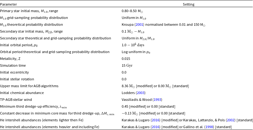
We find that $\Delta M_\textrm{c, min} = -0.13\,\textrm{M}_{\odot}$
and
$\Delta M_\textrm{c, min} = -0.13\,\textrm{M}_{\odot}$
and $\lambda_\textrm{min} = 0.45$
results in the best fitting CSLF to observations from Abia et al. (Reference Abia, de Laverny, Romero-Gómez and Figueras2022), as shown in Fig. 1, together with the fits for
$\lambda_\textrm{min} = 0.45$
results in the best fitting CSLF to observations from Abia et al. (Reference Abia, de Laverny, Romero-Gómez and Figueras2022), as shown in Fig. 1, together with the fits for $(\Delta M_\textrm{c, min}/\,\textrm{M}_{\odot}, \lambda_\textrm{ min}) = ({-}0.12, 0.4)$
,
$(\Delta M_\textrm{c, min}/\,\textrm{M}_{\odot}, \lambda_\textrm{ min}) = ({-}0.12, 0.4)$
, $({-}0.14, 0.5)$
, and (0, 0) shown for comparison. Based on our binning in Fig. 1, the absolute bolometric magnitudes of our C-star population range between
$({-}0.14, 0.5)$
, and (0, 0) shown for comparison. Based on our binning in Fig. 1, the absolute bolometric magnitudes of our C-star population range between $-3.45$
to
$-3.45$
to $-6.75$
mag and peaks at
$-6.75$
mag and peaks at $-4.8$
mag, as observed in Abia et al. (Reference Abia, de Laverny, Romero-Gómez and Figueras2022), but it also over-predicts the low-luminosity tail and under-predicts the high-luminosity tail of the observed distribution.
$-4.8$
mag, as observed in Abia et al. (Reference Abia, de Laverny, Romero-Gómez and Figueras2022), but it also over-predicts the low-luminosity tail and under-predicts the high-luminosity tail of the observed distribution.
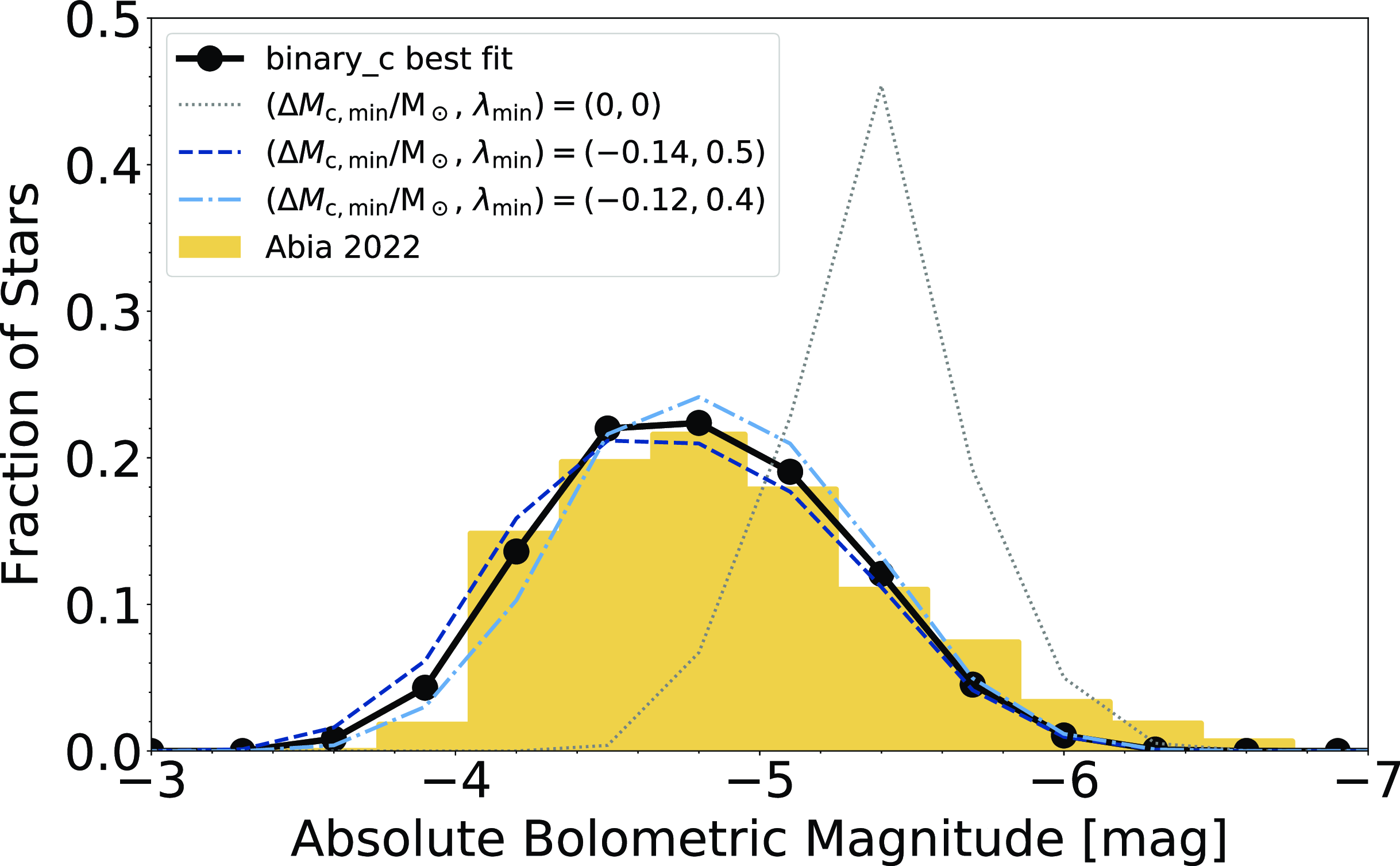
Figure 1. Our best-fit to the CSLF presented in Abia et al. (Reference Abia, de Laverny, Romero-Gómez and Figueras2022) results when $(\Delta M_\textrm{c,min}/\,\textrm{M}_{\odot}, \lambda_\textrm{min}) = ({-}0.13, 0.45)$
. We include the results for (
$(\Delta M_\textrm{c,min}/\,\textrm{M}_{\odot}, \lambda_\textrm{min}) = ({-}0.13, 0.45)$
. We include the results for ( $M_\textrm{c,min}/\,\textrm{M}_{\odot}, \lambda_\textrm{min}) ={} ({-}0.12, 0.4)$
,
$M_\textrm{c,min}/\,\textrm{M}_{\odot}, \lambda_\textrm{min}) ={} ({-}0.12, 0.4)$
, $(0.14, 0.5)$
, and (0,0).
$(0.14, 0.5)$
, and (0,0).
Fig. 2 shows that stars of mass 1.2–4.8 M $_{\odot}$
become C-rich, with some stars of mass
$_{\odot}$
become C-rich, with some stars of mass $\gtrsim 7\,\textrm{M}_{\odot}$
becoming C-rich near the end of the TP-AGB after the stellar winds eject enough of the envelope for hot-bottom burning to shut down, ceasing C-destruction via the CNO cycles. Stars modelled using the standard version of binary_c instead become C-rich at initial masses greater than
$\gtrsim 7\,\textrm{M}_{\odot}$
becoming C-rich near the end of the TP-AGB after the stellar winds eject enough of the envelope for hot-bottom burning to shut down, ceasing C-destruction via the CNO cycles. Stars modelled using the standard version of binary_c instead become C-rich at initial masses greater than $1.9\,\textrm{M}_{\odot}$
. Our modifications introduced in Paper I remove the unrealistic spike around
$1.9\,\textrm{M}_{\odot}$
. Our modifications introduced in Paper I remove the unrealistic spike around $7.5\,\textrm{M}_{\odot}$
star. Moreover, the modified binary_c stellar models are more C-rich at masses
$7.5\,\textrm{M}_{\odot}$
star. Moreover, the modified binary_c stellar models are more C-rich at masses $\lesssim3.5\,\textrm{M}_{\odot}$
than the stars modelled directly by K16, due to the choice of the parameters
$\lesssim3.5\,\textrm{M}_{\odot}$
than the stars modelled directly by K16, due to the choice of the parameters $\Delta M_\textrm{c, min}$
and
$\Delta M_\textrm{c, min}$
and $\lambda_\textrm{min}$
in binary_c being applied regardless of the initial stellar mass.
$\lambda_\textrm{min}$
in binary_c being applied regardless of the initial stellar mass.

Figure 2. Final surface C/O ratios of single stars from K16, and the standard and modified versions of binary_c, and our modified version of binary_c. The C/O ratio = 1 is marked to highlight stars that end their lives C-rich.
A minimum C star mass of $1.2\,\textrm{M}_{\odot}$
is low compared to other model predictions, which estimate
$1.2\,\textrm{M}_{\odot}$
is low compared to other model predictions, which estimate $\sim$ $1.5\,\textrm{M}_{\odot}$
(Marigo Reference Marigo2001; Karakas Reference Karakas2014; Ventura et al. Reference Ventura and Karakas2018). Observations estimate the minimum C star mass to be
$1.5\,\textrm{M}_{\odot}$
(Marigo Reference Marigo2001; Karakas Reference Karakas2014; Ventura et al. Reference Ventura and Karakas2018). Observations estimate the minimum C star mass to be $\sim$ $1.3-1.5\,\textrm{M}_{\odot}$
, although this is uncertain due to the distances to Galactic stars (Pal & Worthey Reference Pal and Worthey2021; Abia et al. Reference Abia, de Laverny, Romero-Gómez and Figueras2022). Fig. 2 shows stars of mass
$1.3-1.5\,\textrm{M}_{\odot}$
, although this is uncertain due to the distances to Galactic stars (Pal & Worthey Reference Pal and Worthey2021; Abia et al. Reference Abia, de Laverny, Romero-Gómez and Figueras2022). Fig. 2 shows stars of mass $\gtrsim5\,\textrm{M}_{\odot}$
often do not become C rich when modelled using the modified version of binary_c, which potentially puts too much weight on low-mass stars to produce the CSLF. Model parameters we have not explored which influence the theoretical CSLF, and therefore the third dredge-up, include the envelope mass where the third dredge-up ceases, which is set to
$\gtrsim5\,\textrm{M}_{\odot}$
often do not become C rich when modelled using the modified version of binary_c, which potentially puts too much weight on low-mass stars to produce the CSLF. Model parameters we have not explored which influence the theoretical CSLF, and therefore the third dredge-up, include the envelope mass where the third dredge-up ceases, which is set to $0.5\,\textrm{M}_{\odot}$
, the duration of hot-bottom burning, the luminosity of AGB stars, and the depth and duration of the luminosity dips approximation described in Equation (5). Therefore, the third dredge-up remains a considerable source of uncertainty in our models.
$0.5\,\textrm{M}_{\odot}$
, the duration of hot-bottom burning, the luminosity of AGB stars, and the depth and duration of the luminosity dips approximation described in Equation (5). Therefore, the third dredge-up remains a considerable source of uncertainty in our models.
3.2 Chemical yield from single stars
A natural consequence of our calibration of the third dredge-up and the updates to the He intershell abundances is the alteration of the single-star stellar yields (see Equations 1 and 2) compared to those calculated from the standard version of binary_c. To verify that the stellar yield calculated using our modified version of binary_c are reasonable, we compare them to those calculated from models using the standard version of binary_c, K16, and, for C, to Marigo (Reference Marigo2001).
We first examine the net yield of C shown in Fig. 3. Here, we compare the net C yields from Marigo (Reference Marigo2001) at solar metallicity where the mixing-length parameter is 1.68. For initial masses $\lesssim 4\,\textrm{M}_{\odot}$
, the net C yield from the modified binary_c models closely reflects the yield from Marigo (Reference Marigo2001). This is likely due to Marigo (Reference Marigo2001) using the CSLF of the Large and Small Magellanic Clouds to calibrate third dredge-up in their models. Although the K16 models employ convective overshoot to force their
$\lesssim 4\,\textrm{M}_{\odot}$
, the net C yield from the modified binary_c models closely reflects the yield from Marigo (Reference Marigo2001). This is likely due to Marigo (Reference Marigo2001) using the CSLF of the Large and Small Magellanic Clouds to calibrate third dredge-up in their models. Although the K16 models employ convective overshoot to force their $1.5$
and
$1.5$
and $1.75\,\textrm{ M}_{\odot}$
stars to be C-rich, they do not explicitly attempt to calibrate their models to fit any CSLF.
$1.75\,\textrm{ M}_{\odot}$
stars to be C-rich, they do not explicitly attempt to calibrate their models to fit any CSLF.
Figure 3. Net C ejected our single stars as calculated from the standard and modified versions of binary_c. We compare the net C yield to those calculated from K16 and Marigo (Reference Marigo2001) at solar-metallicity.
Our net C yield is slightly higher at masses $\lesssim 3\,\textrm{M}_{\odot}$
than calculated in Marigo (Reference Marigo2001), and our stars become C-rich at
$\lesssim 3\,\textrm{M}_{\odot}$
than calculated in Marigo (Reference Marigo2001), and our stars become C-rich at $1.2\,\textrm{M}_{\odot}$
, whereas in the models from Marigo (Reference Marigo2001) they become C-rich at
$1.2\,\textrm{M}_{\odot}$
, whereas in the models from Marigo (Reference Marigo2001) they become C-rich at $1.5\,\textrm{M}_{\odot}$
. This discrepancy likely arises due to the different treatments to the third dredge-up. binary_c uses a variable third dredge-up efficiency, while Marigo (Reference Marigo2001) keeps the efficiency constant through the TP-AGB. Additionally, the occurrence of the third dredge-up in the models from Marigo (Reference Marigo2001) is dependent on the temperature at the base of the convective envelope, which is a dependence binary_c lacks. Instead, the binary_c models terminate the third dredge-up at an envelope mass of
$1.5\,\textrm{M}_{\odot}$
. This discrepancy likely arises due to the different treatments to the third dredge-up. binary_c uses a variable third dredge-up efficiency, while Marigo (Reference Marigo2001) keeps the efficiency constant through the TP-AGB. Additionally, the occurrence of the third dredge-up in the models from Marigo (Reference Marigo2001) is dependent on the temperature at the base of the convective envelope, which is a dependence binary_c lacks. Instead, the binary_c models terminate the third dredge-up at an envelope mass of $0.5\,\textrm{M}_{\odot}$
. See Marigo et al. (Reference Marigo, Girardi and Bressan1999) for the details on how the third dredge-up is treated in their models.
$0.5\,\textrm{M}_{\odot}$
. See Marigo et al. (Reference Marigo, Girardi and Bressan1999) for the details on how the third dredge-up is treated in their models.
At masses $\gtrsim 4\,\textrm{M}_{\odot}$
, the stellar yield from our modified version of binary_c more closely resembles the stellar yield from K16 than those of Marigo (Reference Marigo2001). This is expected since our third dredge-up parameters,
$\gtrsim 4\,\textrm{M}_{\odot}$
, the stellar yield from our modified version of binary_c more closely resembles the stellar yield from K16 than those of Marigo (Reference Marigo2001). This is expected since our third dredge-up parameters, $\Delta M_\textrm{c,min}$
and
$\Delta M_\textrm{c,min}$
and $\lambda_\textrm{min}$
, have very little influence at these masses as these stars enter the TP-AGB with sufficient core masses for third dredge-up.
$\lambda_\textrm{min}$
, have very little influence at these masses as these stars enter the TP-AGB with sufficient core masses for third dredge-up.
The elements produced by the s-process are affected by both the updated He intershell abundances and the new third dredge-up calibration. Fig. 4 shows the net Ba yield from our single-star models. By construction, models from the modified binary_c better agree with K16 than those calculated using the standard binary_c. However, the Ba yield calculated by the modified version of binary_c is higher than those from K16 in the mass range $\sim$
1.3–3.8 M
$\sim$
1.3–3.8 M $_{\odot}$
with a peak at
$_{\odot}$
with a peak at $\sim$ $3\,\textrm{M}_{\odot}$
roughly two times higher. This is due to the third dredge-up calibration, which increases the number and efficiency of third dredge-up.
$3\,\textrm{M}_{\odot}$
roughly two times higher. This is due to the third dredge-up calibration, which increases the number and efficiency of third dredge-up.
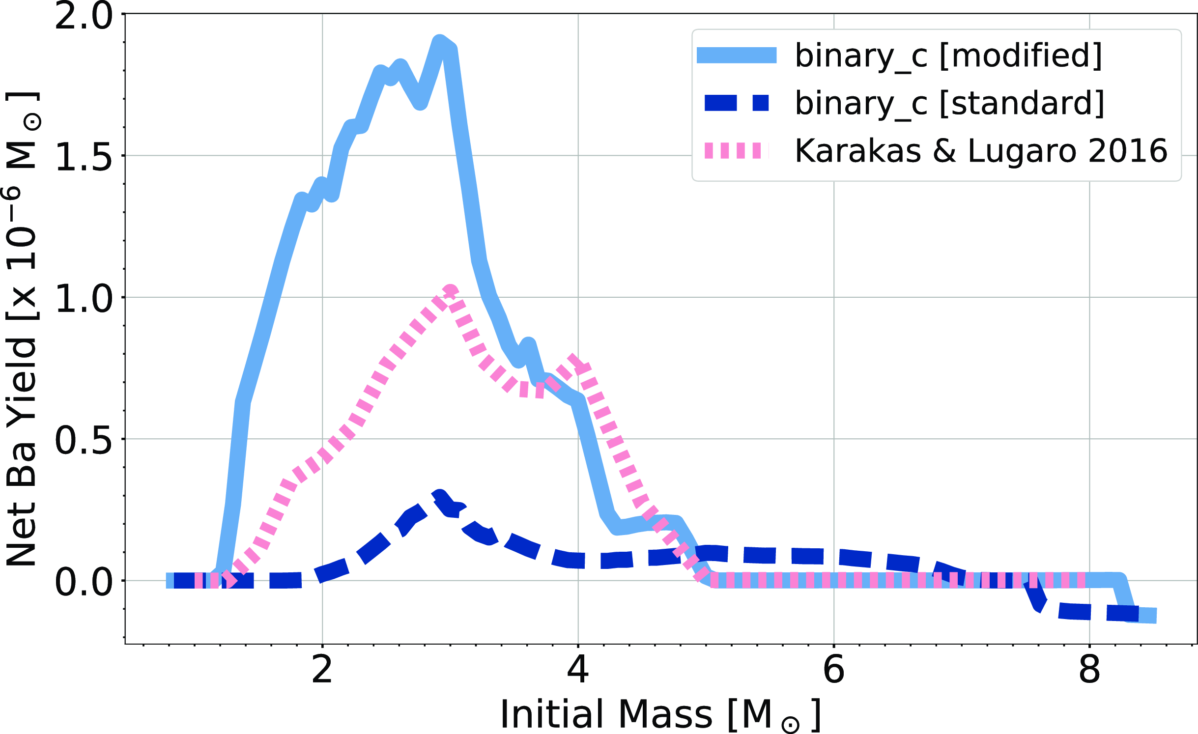
Figure 4. Net Ba yield from single AGB stars calculated from the standard and modified versions of binary_c compared to K16. Our modified version produces a similar Ba yield compared to K16. The standard version of binary_c achieves a peak Ba yield of $3.3 \times 10^{-7} \,\textrm{ M}_{\odot}$
at
$3.3 \times 10^{-7} \,\textrm{ M}_{\odot}$
at $2.9\,\textrm{M}_{\odot}$
, which is a factor of 3.1 times lower than the peak Ba yield from K16 of
$2.9\,\textrm{M}_{\odot}$
, which is a factor of 3.1 times lower than the peak Ba yield from K16 of $1.1 \times 10^{-6} \,\textrm{M}_{\odot}$
at
$1.1 \times 10^{-6} \,\textrm{M}_{\odot}$
at $3\,\textrm{M}_{\odot}$
. The modified version of binary_c has a peak Ba yield of
$3\,\textrm{M}_{\odot}$
. The modified version of binary_c has a peak Ba yield of $1.9\times10^{-6}\,\textrm{M}_{\odot}$
, almost twice as high as the peak K16 Ba yield.
$1.9\times10^{-6}\,\textrm{M}_{\odot}$
, almost twice as high as the peak K16 Ba yield.
Fig. 5 shows the total yields (see Equation 1) of all our considered elements from Fe to Bi for a $2\,\textrm{M}_{\odot}$
star from K16, and the standard and modified binary_c. Fig. 5 highlights that all yields of elements heavier than and including Ga are systemically increased in the modified binary_c results compared to the yields from the
$2\,\textrm{M}_{\odot}$
star from K16, and the standard and modified binary_c. Fig. 5 highlights that all yields of elements heavier than and including Ga are systemically increased in the modified binary_c results compared to the yields from the $2\,\textrm{ M}_{\odot}$
K16 models. The
$2\,\textrm{ M}_{\odot}$
K16 models. The $2\,\textrm{M}_{\odot}$
example star shown is one of the more extreme examples of disagreement between the modified binary_c models and the models from K16, even though stars of this mass experience third dredge-up in both cases. The increased yields result from our third dredge-up calibration, and this is reduced at higher masses owing to their more massive cores and thinner He-intershells. Most elemental yields calculated from modified binary_c are within a factor of 3.6 times the yields from the K16 models. In contrast, the yields calculated from the standard version of binary_c
$2\,\textrm{M}_{\odot}$
example star shown is one of the more extreme examples of disagreement between the modified binary_c models and the models from K16, even though stars of this mass experience third dredge-up in both cases. The increased yields result from our third dredge-up calibration, and this is reduced at higher masses owing to their more massive cores and thinner He-intershells. Most elemental yields calculated from modified binary_c are within a factor of 3.6 times the yields from the K16 models. In contrast, the yields calculated from the standard version of binary_c $2\,\textrm{M}_{\odot}$
model (which includes fits to the He intershell to models by Gallino et al. Reference Gallino, Arlandini, Busso, Lugaro, Travaglio, Straniero, Chieffi and Limongi1998) show a systematic under-production compared to the
$2\,\textrm{M}_{\odot}$
model (which includes fits to the He intershell to models by Gallino et al. Reference Gallino, Arlandini, Busso, Lugaro, Travaglio, Straniero, Chieffi and Limongi1998) show a systematic under-production compared to the $2\,\textrm{M}_{\odot}$
K16 model for all elements including and heavier than Kr. Some key elements from the
$2\,\textrm{M}_{\odot}$
K16 model for all elements including and heavier than Kr. Some key elements from the $2\,\textrm{M}_{\odot}$
standard binary_c model, such as Ba, Ce, and Pb, are under-produced by a factor of 8–10 times the
$2\,\textrm{M}_{\odot}$
standard binary_c model, such as Ba, Ce, and Pb, are under-produced by a factor of 8–10 times the $2\,\textrm{M}_{\odot}$
K16 model. Fig. 4 shows the standard version of binary_c under-produces Ba for all masses <
$2\,\textrm{M}_{\odot}$
K16 model. Fig. 4 shows the standard version of binary_c under-produces Ba for all masses < $4.5\,\textrm{M}_{\odot}$
. The under-production is mainly attributed to the differing treatments of the
$4.5\,\textrm{M}_{\odot}$
. The under-production is mainly attributed to the differing treatments of the ${}^{13}\textrm{C}$
pocket (see Section 2.2).
${}^{13}\textrm{C}$
pocket (see Section 2.2).
3.3 Stellar population yields and abundances
To investigate how binary evolution influences the stellar yield from low- and intermediate-mass populations, we first examine how the binary_c stars evolve. Binary interactions, such as common envelope and Roche-lobe overflow events, may lead to the truncation of stellar evolution. Of particular interest is whether our stars experience the GB, E-AGB, and TP-AGB (at least five thermal pulses), as these evolutionary phases are the sites of the dredge-up episodes that allow low- and intermediate-stars to contribute to the chemical enrichment of the universe. Whether the TP-AGB stars have sufficient mass for hot-bottom burning when they enter the TP-AGB is also of interest, as this process influences the stellar yield of intermediate-mass stars. We use a mass of at least $5\,\textrm{M}_{\odot}$
to indicate a hot-bottom burning star, but the binary_c models show some hot-bottom burning in single stars of mass as low as about
$5\,\textrm{M}_{\odot}$
to indicate a hot-bottom burning star, but the binary_c models show some hot-bottom burning in single stars of mass as low as about $4.5\,\textrm{M}_{\odot}$
. Binary evolution may lead to
$4.5\,\textrm{M}_{\odot}$
. Binary evolution may lead to $4.5\,\textrm{M}_{\odot}$
stars with envelopes too cool for HBB, so we use
$4.5\,\textrm{M}_{\odot}$
stars with envelopes too cool for HBB, so we use $5\,\textrm{M}_{\odot}$
as a more conservative estimate. We show these results in Table 2. Hereafter, unless otherwise specified, all results and discussion are based on calculations made using the modified version of binary_c for a grid of
$5\,\textrm{M}_{\odot}$
as a more conservative estimate. We show these results in Table 2. Hereafter, unless otherwise specified, all results and discussion are based on calculations made using the modified version of binary_c for a grid of $\mbox{1000}$
single and
$\mbox{1000}$
single and $\mbox{640000}$
(
$\mbox{640000}$
( $M_\textrm{1,0}: 100 \times$ $M_\textrm{2,0}:80 \times$ $p_{\rm 0}:80$
) binary stars, sampled as described in Table 1.
$p_{\rm 0}:80$
) binary stars, sampled as described in Table 1.
Table 2. Percentages of single and binary systems (weighted using the birth mass distribution from Kroupa Reference Kroupa2001) with at least one star experiencing the GB, E-AGB, and TP-AGB (at least five thermal pulses) phases and have sufficient mass ( $ \gt $ $5\,\textrm{M}_{\odot}$
) for hot-bottom burning (HBB).
$5\,\textrm{M}_{\odot}$
) for hot-bottom burning (HBB).
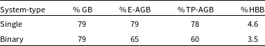
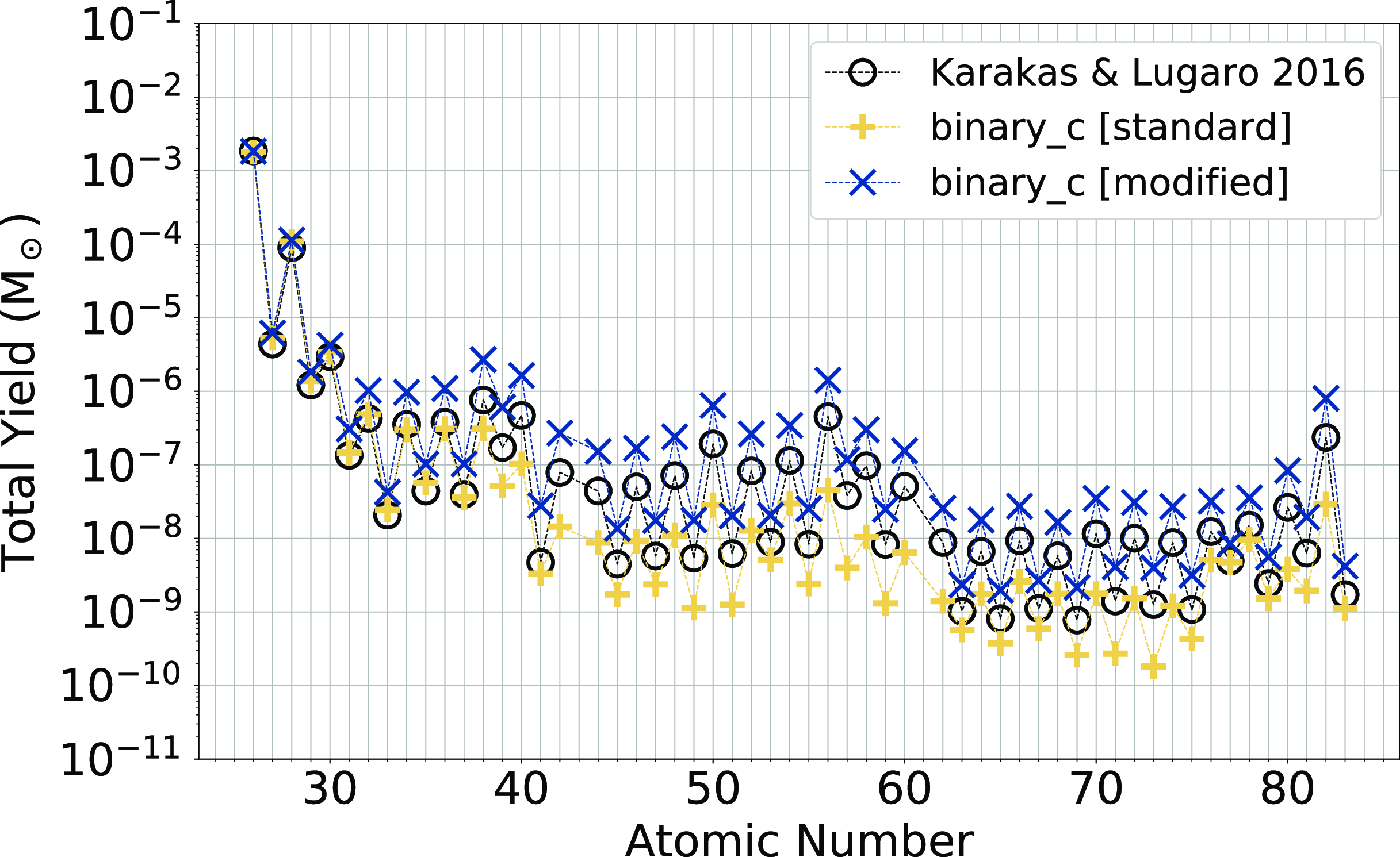
Figure 5. Elemental yields ejected by a $2\,\textrm{M}_{\odot}$
star as calculated by K16, the standard version of binary_c and the modified version of binary_c. We show the elemental yields for all elements from Fe to Bi, excluding radioactive Tc (not reported in K16).
$2\,\textrm{M}_{\odot}$
star as calculated by K16, the standard version of binary_c and the modified version of binary_c. We show the elemental yields for all elements from Fe to Bi, excluding radioactive Tc (not reported in K16).
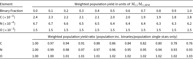
Table 3. C, N, and O stellar population yield ejected by low- and intermediate-mass stellar populations with varying binary fractions. We also show the ratios between the C, N, and O yields produced by populations including binary systems divided by the yield produced by the population of single stars only. C is the most heavily influenced by binary evolution as the binary population (binary fraction = 1) produces 24% less C than the population of single stars only.
Due to our lower mass limit of $0.8\,\textrm{M}_{\odot}$
, some stars in our stellar population do not evolve off the main sequence (MS) during the time of the
$0.8\,\textrm{M}_{\odot}$
, some stars in our stellar population do not evolve off the main sequence (MS) during the time of the $15\,$
Gyr simulation. Most single-star systems that do not evolve off the MS are stars of mass
$15\,$
Gyr simulation. Most single-star systems that do not evolve off the MS are stars of mass $\lesssim 0.9\,\textrm{M}_{\odot}$
. As a result, only 79% of our single-star population, and a similar percentage of the binary star population, enters the first giant branch. Not all of these GB stars in binary systems will experience the first dredge-up as the expansion of the stellar radius on the GB makes this phase more likely to experience Roche-lobe overflow than MS and Hertzsprung-Gap (HG) stars.
$\lesssim 0.9\,\textrm{M}_{\odot}$
. As a result, only 79% of our single-star population, and a similar percentage of the binary star population, enters the first giant branch. Not all of these GB stars in binary systems will experience the first dredge-up as the expansion of the stellar radius on the GB makes this phase more likely to experience Roche-lobe overflow than MS and Hertzsprung-Gap (HG) stars.
In general, binary evolution prevents stars from experiencing evolved phases. Compared to the single-star population, we find 17% fewer stars reaching the E-AGB phase in the binary population. A further 23% fewer enters the TP-AGB and experiences at least five thermal pulses. The contributions to the chemical enrichment of the Universe are, on average, limited rather than enhanced by binary interactions. We also find that binary systems contain 24% fewer hot-bottom burning systems than our single-star population, mainly due to fewer systems with TP-AGB stars.
3.3.1 Weighted population yields: C, N, and O
We first examine the stellar yield accounting for our assumed birth distributions (see Table 1) normalised per unit of star-forming material ( $\,\textrm{M}_{\odot}/\textrm{M}_{\odot,\textrm{SFM}}$
) as described in Equation (4), these are hereafter referred to as weighted yield. We then examine the weighted yields of C, N, and O from our population, which are reported in Table 3.
$\,\textrm{M}_{\odot}/\textrm{M}_{\odot,\textrm{SFM}}$
) as described in Equation (4), these are hereafter referred to as weighted yield. We then examine the weighted yields of C, N, and O from our population, which are reported in Table 3.
Fig. 6 shows the carbon yield ejected by two stellar populations with binary fractions 0.0 and 0.7 via stellar winds as a function of the initial primary (or single) star mass. Compared to a population of single stars only, we find that including binaries results in an overall decrease in the weighted C yield. For example, we find an 18% decrease when the binary fraction is 0.7 (see Table 3). C is under-produced because binary evolution sometimes truncates the TP-AGB or completely prevents the formation of a TP-AGB star (see Table 2). We also find a reduction in the formation of C stars as 40% of binary primary stars become a C star compared to 51% in the single-star population.

Figure 6. The weighted C stellar population yield as a function of the single or primary star mass of our single star population and of a population including binaries with a 0.7 binary fraction. We sum and bin all the weighted yields based on the initial primary- or single-star mass. When including binaries, the yield contributions from the single stars, binary primary stars (and post-merger objects), and binary secondary stars are stated in the legend and stacked in the plot, with their summation totalling the yielded carbon from the population. In this case, 28% of the ejected C originates from the single star portion of the population, 53% from the binary primary stars, and 19% from the binary secondary stars.
Although, on average, binary evolution results in an under-production of C, some circumstances allow C overproduction in binary systems. Among low-mass (primary star mass, $M_\textrm{1,0} $
<
$M_\textrm{1,0} $
< $5\,\textrm{M}_{\odot}$
) binary systems, we find the largest C overproduction in stars that experience more thermal pulses than when single. This can happen through binary evolution by mass accretion onto a post-MS star, which forces the accreting star to enter the TP-AGB with a lower core mass and over-massive envelope compared to a single star of identical mass. For intermediate-mass binary systems (
$5\,\textrm{M}_{\odot}$
) binary systems, we find the largest C overproduction in stars that experience more thermal pulses than when single. This can happen through binary evolution by mass accretion onto a post-MS star, which forces the accreting star to enter the TP-AGB with a lower core mass and over-massive envelope compared to a single star of identical mass. For intermediate-mass binary systems ( $5\,\textrm{M}_{\odot} \lt M_\textrm{1,0} $
<
$5\,\textrm{M}_{\odot} \lt M_\textrm{1,0} $
< $8.3\,\textrm{M}_{\odot}$
), mergers between He-WD and CO-WD form objects similar to R Coronae Borealis stars (Clayton Reference Clayton1996; Karakas, Ruiter, & Hampel Reference Karakas, Ruiter and Hampel2015; Tisserand et al. Reference Tisserand2020) which then eject up to about
$8.3\,\textrm{M}_{\odot}$
), mergers between He-WD and CO-WD form objects similar to R Coronae Borealis stars (Clayton Reference Clayton1996; Karakas, Ruiter, & Hampel Reference Karakas, Ruiter and Hampel2015; Tisserand et al. Reference Tisserand2020) which then eject up to about $0.03\,\textrm{M}_{\odot}$
of C, making them the objects with the highest C-overproduction in this mass range.
$0.03\,\textrm{M}_{\odot}$
of C, making them the objects with the highest C-overproduction in this mass range.
The binary star population forms an R Coronae Borealis star at a rate of about $3\,500$
per
$3\,500$
per $10^6\,\textrm{M}_{\odot}$
of binary star-forming material. Our models estimate the average lifetime of an R Coronae Borealis star to be approximately
$10^6\,\textrm{M}_{\odot}$
of binary star-forming material. Our models estimate the average lifetime of an R Coronae Borealis star to be approximately $7 \times 10^5\,\text{yr}$
, which is slightly longer than the
$7 \times 10^5\,\text{yr}$
, which is slightly longer than the $1-3 \times 10^5 \, \text{yr}$
estimated in other studies (Saio & Jeffery Reference Saio and Jeffery2002; Clayton Reference Clayton2012). If we take the lifetime to be 1–7
$1-3 \times 10^5 \, \text{yr}$
estimated in other studies (Saio & Jeffery Reference Saio and Jeffery2002; Clayton Reference Clayton2012). If we take the lifetime to be 1–7 $\times 10^5\,\text{yr}$
, and a constant Milky Way star formation rate of
$\times 10^5\,\text{yr}$
, and a constant Milky Way star formation rate of $2\,\textrm{M}_{\odot}$
per year (Elia et al. Reference Elia2022) at solar-metallicity and a binary fraction of 0.7, we estimate there are approximately
$2\,\textrm{M}_{\odot}$
per year (Elia et al. Reference Elia2022) at solar-metallicity and a binary fraction of 0.7, we estimate there are approximately $\mbox{500-3800}$
R Coronae Borealis stars in the Galaxy today.
$\mbox{500-3800}$
R Coronae Borealis stars in the Galaxy today.
The nitrogen ejected via stellar winds from our low- and intermediate-mass population as a function of initial primary and single star mass is shown in Fig. 7. In low-mass stars, including binaries results in a net overproduction of N despite the reduced number of AGB stars. There are two distinct evolutionary channels responsible for this. The first is mergers resulting in a star with sufficient mass for hot-bottom burning. Also, mass transfer or common envelope ejections that strip the H envelopes from stars with He-rich cores result in He-rich stars with N surface mass fractions of $\sim$ $0.01$
. Stellar winds from these He-rich stars are the second source of N overproduction in low-mass stars. Intermediate-mass stars instead, on average, experience N under-production due to binary evolution since hot-bottom burning is sometimes prevented or suppressed (see Table 2). Table 3 shows that, overall, despite the N overproduction in low-mass stars, binary evolution has little impact on the overall N production from our low- and intermediate-mass stellar population as the overproduction from the low-mass population cancels out the under-production from the intermediate-mass population.
$0.01$
. Stellar winds from these He-rich stars are the second source of N overproduction in low-mass stars. Intermediate-mass stars instead, on average, experience N under-production due to binary evolution since hot-bottom burning is sometimes prevented or suppressed (see Table 2). Table 3 shows that, overall, despite the N overproduction in low-mass stars, binary evolution has little impact on the overall N production from our low- and intermediate-mass stellar population as the overproduction from the low-mass population cancels out the under-production from the intermediate-mass population.
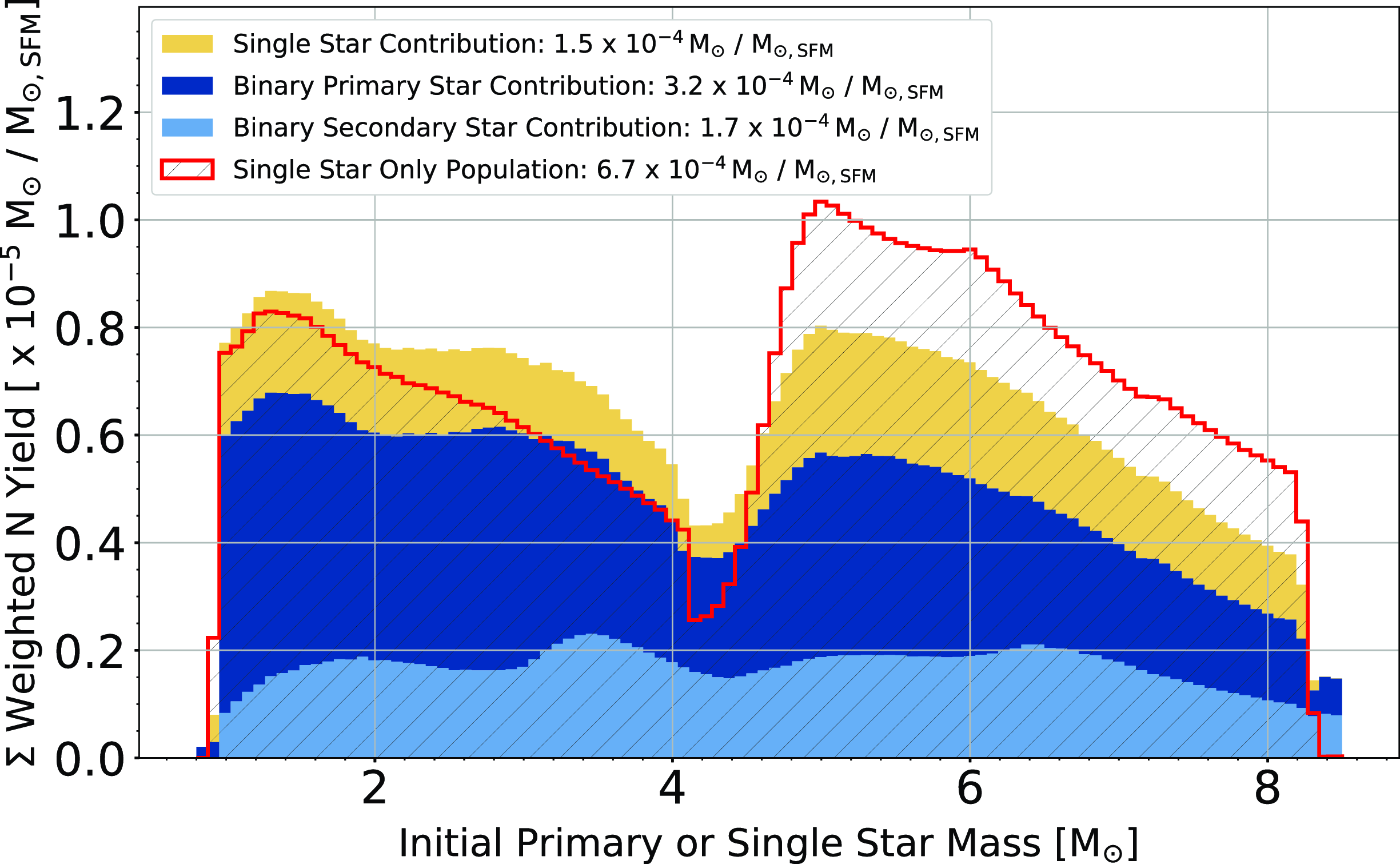
Figure 7. Same as Fig. 6, but for N. For the binary population, 24% of the ejected N originates from the single star portion of the population, 50% from the binary primary stars, and 26% from our binary secondary stars.
We find little deviation of the O yield from our low- and intermediate-mass population (as shown in Table 3). This is expected as most of the O they synthesise remains inside the CO core. Core-collapse supernovae synthesise substantial amounts of oxygen, but we do not include their contribution. The most extreme O producers in the binary population originate from ONe-WDs merging with He-WDs and forming naked-He stars with an O mass fraction of about 0.6, similar to an R Coronae Borealis star but O-rich instead of C-rich. To our knowledge, no such objects have been observed so far, and our models predict them to be rare, with about 5 forming per $10^6\,\textrm{M}_{\odot}$
of star-forming material. These objects survive up to approximately
$10^6\,\textrm{M}_{\odot}$
of star-forming material. These objects survive up to approximately $3\times10^5$
years before finally ejecting their envelopes. Using this lifetime, we estimate up to 2 of these objects are present in the Galaxy today. However, the lifetimes of these objects are highly uncertain as their unique composition would likely influence mass loss.
$3\times10^5$
years before finally ejecting their envelopes. Using this lifetime, we estimate up to 2 of these objects are present in the Galaxy today. However, the lifetimes of these objects are highly uncertain as their unique composition would likely influence mass loss.
3.3.2 Binary system abundance ratios (CNO)
Here, we investigate the statistical distributions of the solar-scaled [C/O], [C/N], and [N/O] ratios of the total material ejected into the interstellar medium and discuss the evolution of binary systems with depleted or enhanced abundance ratios compared to single stars. We calculate the ratios between elements X and Y (abundance by number) using,
 \begin{align} [{X/Y}] = \textrm{log}_{10} \left( \frac{{X}}{{Y}} \right)_\textrm{star} - \textrm{log}_{10} \left( \frac{{X}} {{Y}} \right)_{\odot},\end{align}
where the solar abundances are from Lodders (Reference Lodders2003).
The [C/O] distribution ejected from both our binary and single-star populations is shown in Fig. 8. We calculate the ratios from our binary systems using the total stellar yield combined from the primary and secondary stars. This gives us the distribution of released abundances into the interstellar medium. We find that binary evolution can lead to systems with a lower [C/O] ratio than that in single stars. The lowest [C/O] in our single stars is −0.28, corresponding to an $8.28\,\textrm{M}_{\odot}$
star, and the maximum is +0.94, corresponding to a
$8.28\,\textrm{M}_{\odot}$
star, and the maximum is +0.94, corresponding to a $2.80\,\textrm{M}_{\odot}$
star.
$2.80\,\textrm{M}_{\odot}$
star.

Figure 8. Distribution of [C/O] ratios from our binary and single-star populations released into the interstellar medium.
In our grid of binary models, the minimum [C/O] is −0.90 from the $M_\textrm{1,0} = 8.23\,\textrm{M}_{\odot}$
,
$M_\textrm{1,0} = 8.23\,\textrm{M}_{\odot}$
, $M_\textrm{2,0} = 0.45\,\textrm{M}_{\odot}$
, and
$M_\textrm{2,0} = 0.45\,\textrm{M}_{\odot}$
, and $p_\textrm{0} = 10.0 \, \textrm{yr}$
system, with 0.04% of the systems born in the binary population ejecting [C/O] < −0.38 (0.1 dex lower than the minimum [C/O] ejected by the
$p_\textrm{0} = 10.0 \, \textrm{yr}$
system, with 0.04% of the systems born in the binary population ejecting [C/O] < −0.38 (0.1 dex lower than the minimum [C/O] ejected by the $8.23\,\textrm{M}_{\odot}$
single star). Most of these systems are hot-bottom burning stars with low-mass companions that experience at least one common envelope event. In a single star, hot-bottom burning destroys C in the envelope, but the star recovers some surface C through third dredge-ups after mass loss shuts down hot-bottom burning. There is also some O destruction when the bottom of the convective envelope becomes hot enough to activate NO burning (see Fig. 9). In the binary scenario, a common envelope event might interrupt the TP-AGB primary star when hot-bottom burning has destroyed a large amount of C but not a considerable amount of O. For example, in the case where
$8.23\,\textrm{M}_{\odot}$
single star). Most of these systems are hot-bottom burning stars with low-mass companions that experience at least one common envelope event. In a single star, hot-bottom burning destroys C in the envelope, but the star recovers some surface C through third dredge-ups after mass loss shuts down hot-bottom burning. There is also some O destruction when the bottom of the convective envelope becomes hot enough to activate NO burning (see Fig. 9). In the binary scenario, a common envelope event might interrupt the TP-AGB primary star when hot-bottom burning has destroyed a large amount of C but not a considerable amount of O. For example, in the case where $M_\textrm{1,0} = 8.23\,\textrm{M}_{\odot}$
,
$M_\textrm{1,0} = 8.23\,\textrm{M}_{\odot}$
, $M_\textrm{2,0} = 0.45\,\textrm{M}_{\odot}$
, and
$M_\textrm{2,0} = 0.45\,\textrm{M}_{\odot}$
, and $p_\textrm{0} = 10.0 \, \textrm{yr}$
system, the common envelope event occurs after thermal pulse 14 (as marked in Fig. 9) and ejecting the stellar envelope when the surface [C/O] is −0.97, leaving an ONe-WD remnant. Sometimes, a second common envelope interrupts the secondary star before it enters the TP-AGB or dredges up any large amounts of C, further limiting potential C production.
$p_\textrm{0} = 10.0 \, \textrm{yr}$
system, the common envelope event occurs after thermal pulse 14 (as marked in Fig. 9) and ejecting the stellar envelope when the surface [C/O] is −0.97, leaving an ONe-WD remnant. Sometimes, a second common envelope interrupts the secondary star before it enters the TP-AGB or dredges up any large amounts of C, further limiting potential C production.

Figure 9. Evolution of the surface mass fractions of C, N, and O as a function of thermal pulse count for the single star $8.23\,\textrm{M}_{\odot}$
model. The dotted vertical line indicates thermal pulse 14 where a common envelope event truncates the stellar evolution of a binary system with
$8.23\,\textrm{M}_{\odot}$
model. The dotted vertical line indicates thermal pulse 14 where a common envelope event truncates the stellar evolution of a binary system with $M_\textrm{ 1,0} = 8.23\,\textrm{M}_{\odot}$
,
$M_\textrm{ 1,0} = 8.23\,\textrm{M}_{\odot}$
, $M_\textrm{2,0} = 0.45\,\textrm{M}_{\odot}$
, and
$M_\textrm{2,0} = 0.45\,\textrm{M}_{\odot}$
, and $p_\textrm{0} = 10.0 \, \textrm{yr}$
.
$p_\textrm{0} = 10.0 \, \textrm{yr}$
.
The ejected [N/O] distributions are shown in Fig. 10. The [N/O] ratios from single stars range from 0.0 (at $0.91\,\textrm{M}_{\odot}$
) to +1.1 (at
$0.91\,\textrm{M}_{\odot}$
) to +1.1 (at $7.26\,\textrm{M}_{\odot}$
). The binary systems instead reach a higher maximum [N/O] ratio of +2.5 in the
$7.26\,\textrm{M}_{\odot}$
). The binary systems instead reach a higher maximum [N/O] ratio of +2.5 in the $M_\textrm{1,0} = 5.46\,\textrm{ M}_{\odot}$
,
$M_\textrm{1,0} = 5.46\,\textrm{ M}_{\odot}$
, $M_\textrm{2,0} = 4.28\,\textrm{M}_{\odot}$
, and
$M_\textrm{2,0} = 4.28\,\textrm{M}_{\odot}$
, and $p_\textrm{0} = 0.09 \, \textrm{yr}$
system, showing that binary evolution can lead to N over-production. We find 0.5% of systems in our binary star population produce [N/O] abundance ratios
$p_\textrm{0} = 0.09 \, \textrm{yr}$
system, showing that binary evolution can lead to N over-production. We find 0.5% of systems in our binary star population produce [N/O] abundance ratios $ \gt +1.2$
, which is 0.1 dex higher than the maximum [N/O] achieved by the single stars. Additionally,
$ \gt +1.2$
, which is 0.1 dex higher than the maximum [N/O] achieved by the single stars. Additionally, $0.01\%$
of the systems in the binary population achieve an [N/O] abundance ratio over +2.2, which is 1 dex higher than achieved by single stars. Most of these N-enhanced binary systems have stars that enter the TP-AGB with over-massive envelopes relative to their core masses due to stellar wind accretion or a merger with a post-MS star. These relatively massive envelopes cause the star to shrink, slowing down mass loss and consequently allowing stars to spend longer in the hot-bottom burning phase than single stars of identical mass. We discussed this in more detail in Paper I.
$0.01\%$
of the systems in the binary population achieve an [N/O] abundance ratio over +2.2, which is 1 dex higher than achieved by single stars. Most of these N-enhanced binary systems have stars that enter the TP-AGB with over-massive envelopes relative to their core masses due to stellar wind accretion or a merger with a post-MS star. These relatively massive envelopes cause the star to shrink, slowing down mass loss and consequently allowing stars to spend longer in the hot-bottom burning phase than single stars of identical mass. We discussed this in more detail in Paper I.

Figure 10. As Fig. 8, but for [N/O].
The ejected [C/N] distribution is shown in Fig. 11. The distributions from our binary- and single-star populations are similar. The minimum [C/N] is -1.7, from the $M_\textrm{1,0} = 7.61\,\textrm{M}_{\odot}$
,
$M_\textrm{1,0} = 7.61\,\textrm{M}_{\odot}$
, $M_\textrm{2,0} = 0.62\,\textrm{M}_{\odot}$
, and
$M_\textrm{2,0} = 0.62\,\textrm{M}_{\odot}$
, and $p_\textrm{0} = 11.9 \, \textrm{yr}$
binary system. This system evolves similarly to the
$p_\textrm{0} = 11.9 \, \textrm{yr}$
binary system. This system evolves similarly to the $M_\textrm{1,0} = 8.23\,\textrm{M}_{\odot}$
,
$M_\textrm{1,0} = 8.23\,\textrm{M}_{\odot}$
, $M_\textrm{2,0} = 0.86\,\textrm{M}_{\odot}$
, and
$M_\textrm{2,0} = 0.86\,\textrm{M}_{\odot}$
, and $p_\textrm{0} = 10.0 \, \textrm{yr}$
case previously discussed. It experiences a common envelope event after the primary star experiences 25 thermal pulses, truncating the TP-AGB phase following the destruction of the carbon in its envelope. The secondary star does not evolve off the MS before the end of the simulation. The maximum [C/N] achieved by our binary systems is +0.75 from our
$p_\textrm{0} = 10.0 \, \textrm{yr}$
case previously discussed. It experiences a common envelope event after the primary star experiences 25 thermal pulses, truncating the TP-AGB phase following the destruction of the carbon in its envelope. The secondary star does not evolve off the MS before the end of the simulation. The maximum [C/N] achieved by our binary systems is +0.75 from our $M_\textrm{1,0} = 1.38\,\textrm{ M}_{\odot}$
,
$M_\textrm{1,0} = 1.38\,\textrm{ M}_{\odot}$
, $M_\textrm{2,0} = 1.37\,\textrm{M}_{\odot}$
, and
$M_\textrm{2,0} = 1.37\,\textrm{M}_{\odot}$
, and $p_\textrm{0} = 1 \, \textrm{d}$
. This system merges while the primary star crosses the HG and the secondary is on the MS, producing a
$p_\textrm{0} = 1 \, \textrm{d}$
. This system merges while the primary star crosses the HG and the secondary is on the MS, producing a $2.74\,\textrm{M}_{\odot}$
star, which then evolves similarly to a single
$2.74\,\textrm{M}_{\odot}$
star, which then evolves similarly to a single $2.74\,\textrm{M}_{\odot}$
star but transports less N to the surface during the first dredge-up due to the star’s under-massive core.
$2.74\,\textrm{M}_{\odot}$
star but transports less N to the surface during the first dredge-up due to the star’s under-massive core.

Figure 11. As Fig. 8, but for [C/N].
3.3.3 Weighted population yield and binary star abundances of the s-process elements
Here, we present results for Sr, Ba, and Pb. These three elements are representative of the three s-process peaks at the magic neutron numbers 50 (Sr), 82 (Ba), and 126 (Pb). Similarly to our previous analysis of C, N, and O, we first look at how including binary stars alters the Sr, Ba, and Pb stellar yield compared with a stellar population composed of single-star systems only. We then examine the ejected [Ba/Fe] abundance ratios and discuss enhancements and depletion due to binary evolution.
Table 4 shows the weighted stellar yields of Sr, Ba, and Pb ejected by stellar populations with various binary fractions. Because we find that binary evolution decreases the population yield of all Sr, Ba, and Pb by about 30%, hereafter, we will focus primarily on Ba. Fig. 12 shows the weighted population yield of Ba as a function of the initial primary and single star mass for the population of single stars only and the population with a binary fraction of 0.7. At this binary fraction, the population ejects 25% less Ba than our population of single stars only. Most Ba under-production occurs in binary systems with initial primary masses of $\sim$ $1.2-4.2\,\textrm{M}_{\odot}$
. It is caused by binary evolution either truncating or preventing stars from entering the TP-AGB, similarly to the case of C.
$1.2-4.2\,\textrm{M}_{\odot}$
. It is caused by binary evolution either truncating or preventing stars from entering the TP-AGB, similarly to the case of C.
Table 4. Weighted Sr, Ba, and Pb stellar yield ejected by the low and intermediate-mass stellar populations of varying binary fractions. We also show the ratio of the yield produced including binaries divided by the population yield produced single stars only.
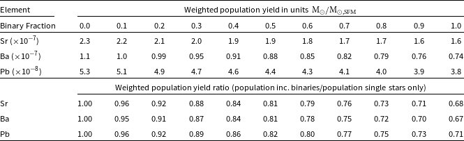
Fig. 13 shows the distribution (per $\mathrm{M}_\mathrm{\odot, SFM}$
) of the [Ba/Fe] abundance ratios in total material ejected into the interstellar medium by the binary- and single-star populations. As in Figs. 8, 10, and 11, the [Ba/Fe] for each stellar system was calculated using the total stellar yield of each system. The maximum [Ba/Fe] achieved by the single-star population is +1.8 at
$\mathrm{M}_\mathrm{\odot, SFM}$
) of the [Ba/Fe] abundance ratios in total material ejected into the interstellar medium by the binary- and single-star populations. As in Figs. 8, 10, and 11, the [Ba/Fe] for each stellar system was calculated using the total stellar yield of each system. The maximum [Ba/Fe] achieved by the single-star population is +1.8 at $1.78\,\textrm{M}_{\odot}$
. The maximum [Ba/Fe] achieved by the binary star population is +2.1 from the
$1.78\,\textrm{M}_{\odot}$
. The maximum [Ba/Fe] achieved by the binary star population is +2.1 from the $M_\textrm{1,0} = 2.60\,\textrm{M}_{\odot}$
,
$M_\textrm{1,0} = 2.60\,\textrm{M}_{\odot}$
, $M_\textrm{2,0} = 1.52\,\textrm{M}_{\odot}$
, and
$M_\textrm{2,0} = 1.52\,\textrm{M}_{\odot}$
, and $p_\textrm{0} = 0.03 \, \textrm{yr}$
system. This system merges while the primary is on the GB and the secondary is on the MS. The merged star has a total mass of
$p_\textrm{0} = 0.03 \, \textrm{yr}$
system. This system merges while the primary is on the GB and the secondary is on the MS. The merged star has a total mass of $3.75\,\textrm{M}_{\odot}$
and a core mass of
$3.75\,\textrm{M}_{\odot}$
and a core mass of $0.55\,\textrm{M}_{\odot}$
at its first thermal pulse. This system experiences 53 thermal pulses before transitioning into a CO-WD, which is 28 more thermal pulses and 31 more third dredge-up events than the corresponding single
$0.55\,\textrm{M}_{\odot}$
at its first thermal pulse. This system experiences 53 thermal pulses before transitioning into a CO-WD, which is 28 more thermal pulses and 31 more third dredge-up events than the corresponding single $3.75\,\textrm{M}_{\odot}$
star. The extra third dredge-up events allow more Ba to be synthesised, transported to the stellar surface, and then ejected by stellar winds.
$3.75\,\textrm{M}_{\odot}$
star. The extra third dredge-up events allow more Ba to be synthesised, transported to the stellar surface, and then ejected by stellar winds.
3.4 Supernovae and Black Holes
Mergers and mass transfer can lead to the initially low- and intermediate-mass stars gaining sufficient mass ( $\gtrsim$ $8.3\,\textrm{M}_{\odot}$
) to end their lives via supernovae. Only 1% of the systems in the binary population experience at least one supernova. These supernovae are mostly Type-II core collapse (Limongi & Chieffi Reference Limongi and Chieffi2018), and Type Ib and c stripped core collapse supernovae (Yoon, Woosley, & Langer Reference Yoon, Woosley and Langer2010).
$8.3\,\textrm{M}_{\odot}$
) to end their lives via supernovae. Only 1% of the systems in the binary population experience at least one supernova. These supernovae are mostly Type-II core collapse (Limongi & Chieffi Reference Limongi and Chieffi2018), and Type Ib and c stripped core collapse supernovae (Yoon, Woosley, & Langer Reference Yoon, Woosley and Langer2010).

Figure 12. As Fig. 6, but for Ba. We find our population of only single stars ejects a weighted Ba stellar yield of $1.1 \times 10^{-7} \, \,\textrm{M}_{\odot}/\textrm{M}_{\odot, \textrm{SFM}}$
. At a binary fraction of 0.7, our population yields
$1.1 \times 10^{-7} \, \,\textrm{M}_{\odot}/\textrm{M}_{\odot, \textrm{SFM}}$
. At a binary fraction of 0.7, our population yields $0.82 \times 10^{-7} \, \,\textrm{M}_{\odot}/\textrm{M}_{\odot, \textrm{SFM}}$
of Ba. From our population, including binaries, 30% of the total ejected Ba originates from the single star portion of the population, 50% from our binary primary stars, and 20% from our binary secondaries.
$0.82 \times 10^{-7} \, \,\textrm{M}_{\odot}/\textrm{M}_{\odot, \textrm{SFM}}$
of Ba. From our population, including binaries, 30% of the total ejected Ba originates from the single star portion of the population, 50% from our binary primary stars, and 20% from our binary secondaries.

Figure 13. As Fig. 8, but for [Ba/Fe]. We find that 0.2% of the stars in our binary population have a [Ba/Fe] ratio > 1.9.
An interesting result from our models is the formation of black holes. Black holes are typically associated with stars of at least $20-25\,\textrm{ M}_{\odot}$
(Fryer Reference Fryer1999; Heger, Müller, & Mandel Reference Heger, Müller and Mandel2023), yet our binary systems can only have a combined maximum mass of
$20-25\,\textrm{ M}_{\odot}$
(Fryer Reference Fryer1999; Heger, Müller, & Mandel Reference Heger, Müller and Mandel2023), yet our binary systems can only have a combined maximum mass of $17\,\textrm{M}_{\odot}$
. Within our binary star population, accretion onto, or a merger with, a neutron star forms five black holes with every
$17\,\textrm{M}_{\odot}$
. Within our binary star population, accretion onto, or a merger with, a neutron star forms five black holes with every $10^6\,\textrm{M}_{\odot}$
of star-forming material (there are 321 in our grid of
$10^6\,\textrm{M}_{\odot}$
of star-forming material (there are 321 in our grid of $\mbox{640000}$
models). The least massive system to form a black hole this way has the initial conditions of
$\mbox{640000}$
models). The least massive system to form a black hole this way has the initial conditions of $M_\textrm{1} = 5.22\,\textrm{M}_{\odot}$
,
$M_\textrm{1} = 5.22\,\textrm{M}_{\odot}$
, $M_\textrm{2} = 5.00\,\textrm{M}_{\odot}$
, and
$M_\textrm{2} = 5.00\,\textrm{M}_{\odot}$
, and $p_\textrm{0} = 58$
days. Stable mass transfer onto the secondary star allows it to gain sufficient mass to explode in a core-collapse supernova forming a neutron star remnant. The neutron star later collapses into a
$p_\textrm{0} = 58$
days. Stable mass transfer onto the secondary star allows it to gain sufficient mass to explode in a core-collapse supernova forming a neutron star remnant. The neutron star later collapses into a $2.24\,\textrm{M}_{\odot}$
black hole after it merges with the CO-WD primary. However, the formation of the black hole is dependent on what is defined as the maximum neutron star mass, which we set to
$2.24\,\textrm{M}_{\odot}$
black hole after it merges with the CO-WD primary. However, the formation of the black hole is dependent on what is defined as the maximum neutron star mass, which we set to $2.2\,\textrm{M}_{\odot}$
(Kalogera & Baym Reference Kalogera and Baym1996; Fan et al. Reference Fan, Han, Jiang, Shao and Tang2024).
$2.2\,\textrm{M}_{\odot}$
(Kalogera & Baym Reference Kalogera and Baym1996; Fan et al. Reference Fan, Han, Jiang, Shao and Tang2024).
Observations support the existence of compact objects of mass $\sim$
2–5 M
$\sim$
2–5 M $_{\odot}$
(Abbott et al. Reference Abbott2020; Wyrzykowski & Mandel Reference Wyrzykowski and Mandel2020), however, their origins remain uncertain. Since our stellar population was not set up to study black hole formation, further study is required to determine the significance of low- and intermediate-mass binary systems as black hole progenitors.
$_{\odot}$
(Abbott et al. Reference Abbott2020; Wyrzykowski & Mandel Reference Wyrzykowski and Mandel2020), however, their origins remain uncertain. Since our stellar population was not set up to study black hole formation, further study is required to determine the significance of low- and intermediate-mass binary systems as black hole progenitors.
4. Comparison to barium stars
We now extend our analysis to compare our models to observations of Galactic Ba stars. Here, we use our stellar-grid of $640\,000$
binary stellar models as described in Section 2.
$640\,000$
binary stellar models as described in Section 2.
Barium stars are giant stars with enriched surface s-process abundances despite not evolving to the AGB (McClure Reference McClure1983; Jorissen et al. Reference Jorissen, Boffin, Karinkuzhi, Van Eck, Escorza, Shetye and VanWinckel2019). They gained their s-process enrichment extrinsically via mass transfer from a TP-AGB companion. In this way, Ba stars preserve the s-process elements from the TP-AGB companion, allowing us to calculate the s-process production of the progenitor TP-AGB star (den Hartogh et al. Reference den Hartogh2023). We can use the observed abundances from Ba stars to test how well our models align with observations.
We identify G and K giants in our modelled binary population as in Izzard, Dermine, & Church (Reference Izzard, Dermine and Church2010). We sample the surface abundances of the secondary stars at the end of the donor star’s AGB, maximising the s-process surface abundances of the Ba star. Since Ba lines are too strong in Ba star spectra for reliable abundance measurements, often other s-process peak elements are used as proxies for Ba, such as Y and La (for example, see de Castro et al. Reference de Castro, Pereira, Roig, Jilinski, Drake, Chavero and Sales Silva2016 and Roriz et al. Reference Roriz, Holanda, da Conceição, Junqueira, Drake, Sonally and Pereira2024). Following these authors, we define a Ba star to have an average surface abundance ratio of [Y/Fe], [La/Fe], [Ce/Fe], and [Nd/Fe] > +0.25, where we calculate the average after calculating the solar-scaled surface abundance ratios using Equation (6). We define mild Ba stars as having an average s-process surface abundance ratio calculated between +0.25 and +1.0 dex. Strong Ba stars are defined to have an average s-process surface abundance ratio [s/Fe] > +1.0 dex.
We use the Ba star sample presented in Cseh et al. (Reference Cseh2018) (derived from de Castro et al. Reference de Castro, Pereira, Roig, Jilinski, Drake, Chavero and Sales Silva2016) to compare to the [Ce/Y] and [Fe/H] surface abundances calculated by our models. From this sample, we only use the 75 stars with [Fe/H] of $0.00$
to
$0.00$
to $+0.05$
dex (including error bars). Additionally, we use the 12 Ba stars presented in Jorissen et al. (Reference Jorissen, Boffin, Karinkuzhi, Van Eck, Escorza, Shetye and VanWinckel2019) with an [Fe/H] from −0.1 to +0.1 dex to compare the stellar masses and orbital periods of our predicted Ba star systems. For our estimate of the number of Ba stars presently in the Milky Way, we assume
$+0.05$
dex (including error bars). Additionally, we use the 12 Ba stars presented in Jorissen et al. (Reference Jorissen, Boffin, Karinkuzhi, Van Eck, Escorza, Shetye and VanWinckel2019) with an [Fe/H] from −0.1 to +0.1 dex to compare the stellar masses and orbital periods of our predicted Ba star systems. For our estimate of the number of Ba stars presently in the Milky Way, we assume $10\,$
Gyr of star formation at a constant star formation rate of
$10\,$
Gyr of star formation at a constant star formation rate of $2\,\textrm{M}_{\odot}/\text{yr}$
at solar-metallicity and a binary fraction of 0.7.
$2\,\textrm{M}_{\odot}/\text{yr}$
at solar-metallicity and a binary fraction of 0.7.
We find approximately $\mbox{8200}$
Ba stars progenitors from every
$\mbox{8200}$
Ba stars progenitors from every $10^6\,\textrm{M}_{\odot}$
of binary-star-forming material, and we estimate a total of
$10^6\,\textrm{M}_{\odot}$
of binary-star-forming material, and we estimate a total of $3.6 \times 10^6$
Ba stars at solar-metallicity currently in the Milky Way.
$3.6 \times 10^6$
Ba stars at solar-metallicity currently in the Milky Way.
Our comparison of the [Ce/Y] surface abundances to the predicted Ba stars to the data from Cseh et al. (Reference Cseh2018) in Fig. 14. The maximum predicted [Ce/Y] abundance ratio is +0.30, and the minimum is $-0.19$
. Of the predicted Ba stars 40% have [Ce/Y] >
$-0.19$
. Of the predicted Ba stars 40% have [Ce/Y] > $+0.2$
, and 60% have −0.2 < [Ce/Y] < +0.2. This distribution favours Ba stars of higher surface [Ce/Y] abundance ratio than the observed distribution, which has 24% with [Ce/Y] > +0.2, 73% with −0.2 < [Ce/Y] < +0.4, and 3% with [Ce/Y] < −0.4, not taking observational error into account. Restricting the star-formation time to
$+0.2$
, and 60% have −0.2 < [Ce/Y] < +0.2. This distribution favours Ba stars of higher surface [Ce/Y] abundance ratio than the observed distribution, which has 24% with [Ce/Y] > +0.2, 73% with −0.2 < [Ce/Y] < +0.4, and 3% with [Ce/Y] < −0.4, not taking observational error into account. Restricting the star-formation time to $5\,$
Gyr results in 36% of Ba Stars with [Ce/Y] >
$5\,$
Gyr results in 36% of Ba Stars with [Ce/Y] > $+0.2$
, and 64% having −0.2 < [Ce/Y] < +0.2. Additionally, because the observed minimum of [Ce/Y]
$+0.2$
, and 64% having −0.2 < [Ce/Y] < +0.2. Additionally, because the observed minimum of [Ce/Y] $= -0.3$
, we cannot reproduce these 3% of Ba stars within
$= -0.3$
, we cannot reproduce these 3% of Ba stars within $1\sigma$
of observational errors.
$1\sigma$
of observational errors.

Figure 14. [Ce/Y] and [Fe/H] (left) surface abundances and the [Ce/Y] distribution (right) of the predicted Ba stars compared to observed Ba stars reported in Cseh et al. (Reference Cseh2018). The plots share the same y-axis.
The masses, orbital periods, and frequencies of predicted Ba stars within our binary population are shown in Fig. 15, compared to observations of solar-metallicity Ba stars reported in Jorissen et al. (Reference Jorissen, Boffin, Karinkuzhi, Van Eck, Escorza, Shetye and VanWinckel2019). From our predicted Ba systems, the average WD mass is $0.63\,\textrm{ M}_{\odot}$
, the average Ba star mass is
$0.63\,\textrm{ M}_{\odot}$
, the average Ba star mass is $1.7\,\textrm{M}_{\odot}$
, and the average orbital period is
$1.7\,\textrm{M}_{\odot}$
, and the average orbital period is $3.6\times10^{4}$
days. Jorissen et al. (Reference Jorissen, Boffin, Karinkuzhi, Van Eck, Escorza, Shetye and VanWinckel2019), on average, observe more massive WDs and Ba stars at solar-metallicity than predicted with
$3.6\times10^{4}$
days. Jorissen et al. (Reference Jorissen, Boffin, Karinkuzhi, Van Eck, Escorza, Shetye and VanWinckel2019), on average, observe more massive WDs and Ba stars at solar-metallicity than predicted with $0.81$
and
$0.81$
and $2.9\,\textrm{M}_{\odot}$
, respectively. The predicted orbital periods are longer than observed, with the maximum orbital period calculated in Jorissen et al. (Reference Jorissen, Boffin, Karinkuzhi, Van Eck, Escorza, Shetye and VanWinckel2019) to be
$2.9\,\textrm{M}_{\odot}$
, respectively. The predicted orbital periods are longer than observed, with the maximum orbital period calculated in Jorissen et al. (Reference Jorissen, Boffin, Karinkuzhi, Van Eck, Escorza, Shetye and VanWinckel2019) to be $1.7\times10^4$
days. Our models also estimate that 48% observed solar-metallicity Ba stars are strong Ba stars, but there are only 2 in the sample of 12 from Jorissen et al. (Reference Jorissen, Boffin, Karinkuzhi, Van Eck, Escorza, Shetye and VanWinckel2019).
$1.7\times10^4$
days. Our models also estimate that 48% observed solar-metallicity Ba stars are strong Ba stars, but there are only 2 in the sample of 12 from Jorissen et al. (Reference Jorissen, Boffin, Karinkuzhi, Van Eck, Escorza, Shetye and VanWinckel2019).

Figure 15. Distributions of WD masses (top), Ba star masses (middle) and orbital periods (bottom) for predicted Ba star systems compared to observations from Jorissen et al. (Reference Jorissen, Boffin, Karinkuzhi, Van Eck, Escorza, Shetye and VanWinckel2019). The legend for all three panels is presented in the middle panel.
The distribution in Fig. 15 (middle) shows the formation of a small number (0.08% of all Ba stars) of massive Ba stars with mass $\gtrsim10\,\textrm{M}_{\odot}$
, which is not observed in Jorissen et al. (Reference Jorissen, Boffin, Karinkuzhi, Van Eck, Escorza, Shetye and VanWinckel2019). These Ba stars originate from intermediate-mass binary systems with an initial primary star mass
$\gtrsim10\,\textrm{M}_{\odot}$
, which is not observed in Jorissen et al. (Reference Jorissen, Boffin, Karinkuzhi, Van Eck, Escorza, Shetye and VanWinckel2019). These Ba stars originate from intermediate-mass binary systems with an initial primary star mass $\gtrsim 6\,\textrm{M}_{\odot}$
and
$\gtrsim 6\,\textrm{M}_{\odot}$
and $M_\textrm{2,0}/M_\textrm{1,0} \approx 1$
. Stable mass transfer from the primary to the secondary results in a TP-AGB primary star of mass 1.71–2.25 M
$M_\textrm{2,0}/M_\textrm{1,0} \approx 1$
. Stable mass transfer from the primary to the secondary results in a TP-AGB primary star of mass 1.71–2.25 M $_{\odot}$
with a massive MS companion secondary star. Their primary stars enter the TP-AGB with massive cores compared to single stars of identical mass and experience an elevated number of thermal pulses. None of these systems experience a common envelope event. The resulting Ba star systems have WD masses between 0.95–1.33 M
$_{\odot}$
with a massive MS companion secondary star. Their primary stars enter the TP-AGB with massive cores compared to single stars of identical mass and experience an elevated number of thermal pulses. None of these systems experience a common envelope event. The resulting Ba star systems have WD masses between 0.95–1.33 M $_{\odot}$
, Ba star masses 10.8–14.9 M
$_{\odot}$
, Ba star masses 10.8–14.9 M $_{\odot}$
, and orbital periods of
$_{\odot}$
, and orbital periods of $\mbox{2971-8331}$
days. These massive Ba stars fall under the mild Ba star category and are observable as Ba stars for about 1–3 Myr (6–16 Myr if you include their lifetime while s-process enriched on the MS). We estimate approximately 30 massive Ba stars are presently in the Milky Way. In this context, it is unsurprising that none have been observed, regardless of whether the channel truly occurs in nature.
$\mbox{2971-8331}$
days. These massive Ba stars fall under the mild Ba star category and are observable as Ba stars for about 1–3 Myr (6–16 Myr if you include their lifetime while s-process enriched on the MS). We estimate approximately 30 massive Ba stars are presently in the Milky Way. In this context, it is unsurprising that none have been observed, regardless of whether the channel truly occurs in nature.
5. Discussion
Here, we discuss the uncertainty in our model parameters and the uncertainty the Ba stars models exposed.
5.1. Model uncertainty
AGB and binary evolution have major uncertainties related to mixing and convective boundaries, stellar winds, mass transfer, common envelope evolution, and s-process nucleosynthesis. To discern their impact, we computed stellar populations of binary stars calculated with grids of $\mbox{640000}$
stellar models (
$\mbox{640000}$
stellar models ( $M_\textrm{1,0}\,:\, 100 \times M_\textrm{2,0}\,:\,80 \times p_\textrm{0}\,:\,80$
), varying the model parameters: common envelope efficiency
$M_\textrm{1,0}\,:\, 100 \times M_\textrm{2,0}\,:\,80 \times p_\textrm{0}\,:\,80$
), varying the model parameters: common envelope efficiency $\alpha_\textrm{CE}$
, third dredge-up parameters
$\alpha_\textrm{CE}$
, third dredge-up parameters $\Delta M_\textrm{c, min}$
and
$\Delta M_\textrm{c, min}$
and $\lambda_\textrm{min}$
, TP-AGB mass-loss prescription, Roche-lobe overflow prescription, and wind Roche-Lobe overflow prescription, and compare the weighted C, N, and Ba yield to our stellar population as described in Table 1. Our discussion will primarily focus on Ba as it shows the largest deviations. Fig. 16 shows the results of the variation of these model parameters on the weighted Ba yield.
$\lambda_\textrm{min}$
, TP-AGB mass-loss prescription, Roche-lobe overflow prescription, and wind Roche-Lobe overflow prescription, and compare the weighted C, N, and Ba yield to our stellar population as described in Table 1. Our discussion will primarily focus on Ba as it shows the largest deviations. Fig. 16 shows the results of the variation of these model parameters on the weighted Ba yield.

Figure 16. Percentage difference in the Ba ejected by our binary star population (binary fraction is 1.0) with varying common envelope and third dredge-up parameters, mass-loss rates, the Roche-lobe overflow prescription (changed to Hurley, Tout, & Pols Reference Hurley, Tout and Pols2002, and notated as RLOF BSE prescription), and the wind Roche-lobe overflow (WRLOF) compared to the population calculated using the model parameters described in Table 1. The zero-line corresponds to our models set up as shown in Table 1 where $(\Delta M_\textrm{c, min}/\,\textrm{ M}_{\odot}, \lambda_\textrm{min}) = ({-}0.13, 0.45)$
,
$(\Delta M_\textrm{c, min}/\,\textrm{ M}_{\odot}, \lambda_\textrm{min}) = ({-}0.13, 0.45)$
, $\alpha_\textrm{CE} = 1$
, mass-loss on the TP-AGB as described in Vassiliadis & Wood (Reference Vassiliadis and Wood1993), Roche-lobe overflow as described in Claeys et al. (Reference Claeys, Pols, Izzard, Vink and Verbunt2014), and wind Roche-lobe overflow as described in Abate et al. (Reference Abate, Pols, Izzard, Mohamed and de Mink2013). The population calculated using our chosen model parameters has a total weighted Ba yield of
$\alpha_\textrm{CE} = 1$
, mass-loss on the TP-AGB as described in Vassiliadis & Wood (Reference Vassiliadis and Wood1993), Roche-lobe overflow as described in Claeys et al. (Reference Claeys, Pols, Izzard, Vink and Verbunt2014), and wind Roche-lobe overflow as described in Abate et al. (Reference Abate, Pols, Izzard, Mohamed and de Mink2013). The population calculated using our chosen model parameters has a total weighted Ba yield of $7.4\times 10^{-8} \,\,\textrm{M}_{\odot}/\textrm{M}_{\odot, \textrm{SFM}}$
. In the legend, the quantities in square brackets describe the total weighted Ba yield in units
$7.4\times 10^{-8} \,\,\textrm{M}_{\odot}/\textrm{M}_{\odot, \textrm{SFM}}$
. In the legend, the quantities in square brackets describe the total weighted Ba yield in units $\times 10^{-8}\, \,\textrm{M}_{\odot}/\textrm{M}_{\odot, \textrm{SFM}}$
for each population.
$\times 10^{-8}\, \,\textrm{M}_{\odot}/\textrm{M}_{\odot, \textrm{SFM}}$
for each population.
The common envelope parameter $\alpha_\textrm{CE}$
describes the fraction of orbital energy released by the stellar companion to eject the envelope of a common envelope system (Hurley et al. Reference Hurley, Tout and Pols2002). The higher
$\alpha_\textrm{CE}$
describes the fraction of orbital energy released by the stellar companion to eject the envelope of a common envelope system (Hurley et al. Reference Hurley, Tout and Pols2002). The higher $\alpha_\textrm{CE}$
, the easier it is to eject the envelope in a common envelope event. In Fig. 16, we compare the changes in the weighted Ba yield from our binary population calculated with
$\alpha_\textrm{CE}$
, the easier it is to eject the envelope in a common envelope event. In Fig. 16, we compare the changes in the weighted Ba yield from our binary population calculated with $\alpha_\textrm{CE} = 0.5$
and 2 instead of
$\alpha_\textrm{CE} = 0.5$
and 2 instead of $\alpha_\textrm{CE} = 1$
.
$\alpha_\textrm{CE} = 1$
. $\alpha_\textrm{CE}$
is among the most influential parameters influencing the Ba yield as taking
$\alpha_\textrm{CE}$
is among the most influential parameters influencing the Ba yield as taking $\alpha_\textrm{CE} = 0.5$
results in 10% more merger and TP-AGB progenitor systems and
$\alpha_\textrm{CE} = 0.5$
results in 10% more merger and TP-AGB progenitor systems and $\alpha_\textrm{CE} = 2$
results in 16% fewer mergers 8% fewer TP-AGB progenitors than taking
$\alpha_\textrm{CE} = 2$
results in 16% fewer mergers 8% fewer TP-AGB progenitors than taking $\alpha_\textrm{CE} = 1$
. Altering
$\alpha_\textrm{CE} = 1$
. Altering $\alpha_\textrm{CE}$
to 0.5 and 2 changes the total Ba yield from the binary population by
$\alpha_\textrm{CE}$
to 0.5 and 2 changes the total Ba yield from the binary population by $\pm 10\%$
. Fig. 16 shows the largest deviation in the mass range of about 1–1.2 M
$\pm 10\%$
. Fig. 16 shows the largest deviation in the mass range of about 1–1.2 M $_{\odot}$
, where mergers are essential to Ba production as these stars do not have sufficient mass to experience the third dredge-up or s-process nucleosynthesis when single. C and N increase by 7% when
$_{\odot}$
, where mergers are essential to Ba production as these stars do not have sufficient mass to experience the third dredge-up or s-process nucleosynthesis when single. C and N increase by 7% when $\alpha_\textrm{CE} = 0.5$
, and they decrease by 6% and 3% respectively when
$\alpha_\textrm{CE} = 0.5$
, and they decrease by 6% and 3% respectively when $\alpha_\textrm{CE} = 2$
.
$\alpha_\textrm{CE} = 2$
.
When we force the third dredge-up to begin earlier and with higher minimum efficiency, $(\Delta M_\textrm{c, min}/\,\textrm{M}_{\odot}, \lambda_\textrm{ min}) = ({-}0.14, 0.50)$
, or later and with lower minimum efficiency,
$(\Delta M_\textrm{c, min}/\,\textrm{M}_{\odot}, \lambda_\textrm{ min}) = ({-}0.14, 0.50)$
, or later and with lower minimum efficiency, $(\Delta M_\textrm{c, min}/\,\textrm{M}_{\odot}, \lambda_\textrm{min}) = ({-}0.12, 0.4)$
, than our calibration described in Section 3.1, we find that stars of mass
$(\Delta M_\textrm{c, min}/\,\textrm{M}_{\odot}, \lambda_\textrm{min}) = ({-}0.12, 0.4)$
, than our calibration described in Section 3.1, we find that stars of mass $\lesssim2\,\textrm{M}_{\odot}$
, which eject approximately 80% of the Ba from the binary star population, have the largest deviations in the Ba yield. The largest is a 140% deviation at
$\lesssim2\,\textrm{M}_{\odot}$
, which eject approximately 80% of the Ba from the binary star population, have the largest deviations in the Ba yield. The largest is a 140% deviation at $1.2\,\textrm{M}_{\odot}$
, near the low-mass boundary for the third dredge-up. The total Ba yielded by the binary populations varies by
$1.2\,\textrm{M}_{\odot}$
, near the low-mass boundary for the third dredge-up. The total Ba yielded by the binary populations varies by $\pm 10\%$
. C and N vary by
$\pm 10\%$
. C and N vary by $\pm5\%$
and
$\pm5\%$
and $-0.3\%$
, respectively. The yields from the single-star populations deviate similarly. We find that the C, N, and Ba yield from our binary population change by factors of 0.76, 0.93, and 0.67, respectively, with respect to their corresponding single-star populations, as in Tables 3 and 4, for all treatments of third dredge-up tested here.
$-0.3\%$
, respectively. The yields from the single-star populations deviate similarly. We find that the C, N, and Ba yield from our binary population change by factors of 0.76, 0.93, and 0.67, respectively, with respect to their corresponding single-star populations, as in Tables 3 and 4, for all treatments of third dredge-up tested here.
The mass-loss rate of AGB stars is a major source of uncertainty in AGB star models (Karakas & Lugaro Reference Karakas and Lugaro2016; Höfner & Olofsson Reference Höfner and Olofsson2018). Fig. 16 shows the change in the results using the mass loss prescription described in Bloecker (Reference Bloecker1995) with $\eta = 0.02$
as in Ventura et al. (Reference Ventura and Karakas2018) and Yagüe López et al. (Reference Yagüe López, García-Hernández, Ventura, Doherty, den Hartogh, Jones and Lugaro2022). This stellar wind prescription introduces a deviation of up to 60% in the Ba yield at
$\eta = 0.02$
as in Ventura et al. (Reference Ventura and Karakas2018) and Yagüe López et al. (Reference Yagüe López, García-Hernández, Ventura, Doherty, den Hartogh, Jones and Lugaro2022). This stellar wind prescription introduces a deviation of up to 60% in the Ba yield at $3.76\,\textrm{M}_{\odot}$
, compared to models with the mass-loss described in Table 1. This is because the single
$3.76\,\textrm{M}_{\odot}$
, compared to models with the mass-loss described in Table 1. This is because the single $3.76\,\textrm{M}_{\odot}$
star experiences 24 third dredge-up events with the Bloecker (Reference Bloecker1995) mass loss prescription and 20 third dredge-up events with the Vassiliadis & Wood (Reference Vassiliadis and Wood1993) mass loss prescription. The overall C, N, and Ba weighted yields from the binary population change by
$3.76\,\textrm{M}_{\odot}$
star experiences 24 third dredge-up events with the Bloecker (Reference Bloecker1995) mass loss prescription and 20 third dredge-up events with the Vassiliadis & Wood (Reference Vassiliadis and Wood1993) mass loss prescription. The overall C, N, and Ba weighted yields from the binary population change by $ \lt $
3%. Additionally, when comparing our binary population yield to our single-star population yield, the yields from our binary populations are factors of 0.75, 0.92, and 0.67 of the single star population yield for C, N, and Ba respectively, which is almost identical to the result presented in Tables 3 and 4 when using winds from Vassiliadis & Wood (Reference Vassiliadis and Wood1993).
$ \lt $
3%. Additionally, when comparing our binary population yield to our single-star population yield, the yields from our binary populations are factors of 0.75, 0.92, and 0.67 of the single star population yield for C, N, and Ba respectively, which is almost identical to the result presented in Tables 3 and 4 when using winds from Vassiliadis & Wood (Reference Vassiliadis and Wood1993).
We investigate the effects of changing the Roche-lobe overflow prescription from the prescription described in Claeys et al. (Reference Claeys, Pols, Izzard, Vink and Verbunt2014) to the one described in Hurley et al. (Reference Hurley, Tout and Pols2002). This changes how dynamically stable mass transfer is treated during Roche-lobe overflow. In Hurley et al. (Reference Hurley, Tout and Pols2002), the mass transfer rate is calculated as a function of the amount the Roche-lobe is overfilled (see their Equation 58). The prescription described in Claeys et al. (Reference Claeys, Pols, Izzard, Vink and Verbunt2014) has an additional dependence on the stability of mass transfer (see their Equation 10), which increases the mass transfer rate on the thermal timescale. Using the Roche-lobe overflow prescription described in Hurley et al. (Reference Hurley, Tout and Pols2002) increases the Ba yield by a maximum of 18% at a primary mass of $7.6\,\textrm{ M}_{\odot}$
. It mainly influences binary systems with initial primary mass
$7.6\,\textrm{ M}_{\odot}$
. It mainly influences binary systems with initial primary mass $\gtrsim 5\,\textrm{M}_{\odot}$
where the secondary stars are ejecting most of the Ba. The overall change in the total weighted yield for C, N, and Ba varies by
$\gtrsim 5\,\textrm{M}_{\odot}$
where the secondary stars are ejecting most of the Ba. The overall change in the total weighted yield for C, N, and Ba varies by $ \lt $
3%.
$ \lt $
3%.
Wind Roche-lobe overflow is the efficient mass transfer of stellar wind material gravitationally focused toward the accreting star (Mohamed & Podsiadlowski Reference Mohamed, Podsiadlowski, Napiwotzki and Burleigh2007). Our models use the wind Roche-lobe overflow prescription described in Abate et al. (Reference Abate, Pols, Izzard, Mohamed and de Mink2013). Switching off wind Roche-lobe overflow results in all stellar wind accretion rates calculated from Bondi & Hoyle (Reference Bondi and Hoyle1944). Switching off wind Roche-lobe overflow changes the Ba population yield by a maximum of 30% at a primary mass of $8.23\,\textrm{M}_{\odot}$
as fewer secondary stars accrete sufficient mass for hot-bottom burning, allowing more Ba production. For C and Ba, the variation in the total weighted yield of the population is minimal at
$8.23\,\textrm{M}_{\odot}$
as fewer secondary stars accrete sufficient mass for hot-bottom burning, allowing more Ba production. For C and Ba, the variation in the total weighted yield of the population is minimal at $ \lt $
2%; however, for N, we find a 7% decrease.
$ \lt $
2%; however, for N, we find a 7% decrease.
We do not study the contribution of supernovae to the stellar yield, but from the populations discussed here, we find that using $\alpha_\textrm{CE} = 2$
has the largest influence on their number with a 15% reduction as fewer mergers result in stars with masses
$\alpha_\textrm{CE} = 2$
has the largest influence on their number with a 15% reduction as fewer mergers result in stars with masses $\gtrsim 8.3\,\textrm{M}_{\odot}$
. This is followed by using the Roche-lobe overflow prescription described in Hurley et al. (Reference Hurley, Tout and Pols2002), which reduces the number of supernovae in our population by 10% originating primarily from the secondary stars as they accrete less material than when using the Roche-lobe overflow prescription described in Claeys et al. (Reference Claeys, Pols, Izzard, Vink and Verbunt2014). All other variations to our model population change the number of supernovae by
$\gtrsim 8.3\,\textrm{M}_{\odot}$
. This is followed by using the Roche-lobe overflow prescription described in Hurley et al. (Reference Hurley, Tout and Pols2002), which reduces the number of supernovae in our population by 10% originating primarily from the secondary stars as they accrete less material than when using the Roche-lobe overflow prescription described in Claeys et al. (Reference Claeys, Pols, Izzard, Vink and Verbunt2014). All other variations to our model population change the number of supernovae by $ \lt $
10%.
$ \lt $
10%.
In summary, out of all the sources of uncertainty we investigate here, our settings for $\alpha_\textrm{CE}$
and the third dredge-up introduce the highest overall uncertainty in the Ba yield from our binary population with variations of
$\alpha_\textrm{CE}$
and the third dredge-up introduce the highest overall uncertainty in the Ba yield from our binary population with variations of $\pm 10\%$
each. In the case of C, we find that the
$\pm 10\%$
each. In the case of C, we find that the $\alpha_\textrm{CE}$
parameter introduces the highest uncertainty, with the C yield from our binary population decreasing by 7% when we set
$\alpha_\textrm{CE}$
parameter introduces the highest uncertainty, with the C yield from our binary population decreasing by 7% when we set $\alpha_\textrm{CE} = 2.0$
. For N, wind Roche-lobe overflow has the most influence. We also find that although the third dredge-up treatment and the stellar winds on the TP-AGB alter the total stellar yields, they have little influence on the deviation between the yields from our single-star and binary-star populations, and it is the binary interaction which introduces the most uncertainty in this respect. Other sources of uncertainty we do not explicitly test include convective energy transport in the stellar envelope (which influences dredge-up and hot-bottom burning efficiency, for example, see Boothroyd & Sackmann Reference Boothroyd and Sackmann1988 or Sackmann & Boothroyd Reference Sackmann and Boothroyd1991), the mixing profile of the partial mixing zone (Buntain et al. Reference Buntain, Doherty, Lugaro, Lattanzio, Stancliffe and Karakas2017), and
$\alpha_\textrm{CE} = 2.0$
. For N, wind Roche-lobe overflow has the most influence. We also find that although the third dredge-up treatment and the stellar winds on the TP-AGB alter the total stellar yields, they have little influence on the deviation between the yields from our single-star and binary-star populations, and it is the binary interaction which introduces the most uncertainty in this respect. Other sources of uncertainty we do not explicitly test include convective energy transport in the stellar envelope (which influences dredge-up and hot-bottom burning efficiency, for example, see Boothroyd & Sackmann Reference Boothroyd and Sackmann1988 or Sackmann & Boothroyd Reference Sackmann and Boothroyd1991), the mixing profile of the partial mixing zone (Buntain et al. Reference Buntain, Doherty, Lugaro, Lattanzio, Stancliffe and Karakas2017), and ${}^{13}\textrm{C}$
pocket size.
${}^{13}\textrm{C}$
pocket size.
5.2 Barium star orbital periods and abundances
As described in Section 4, most predicted Galactic Ba stars have surface [Ce/Y] in agreement with observations (Fig. 14). However, Fig. 14 shows we are predicting a higher fraction of Ba stars with [Ce/Y] > +0.2 than observed. 63% of these systems had AGB companions with initial masses $ \lt 1.5\,\textrm{M}_{\odot}$
, outside the mass range of the K16 models with s-process stellar nucleosynthesis. Due to their colder intershells, a star of
$ \lt 1.5\,\textrm{M}_{\odot}$
, outside the mass range of the K16 models with s-process stellar nucleosynthesis. Due to their colder intershells, a star of $1.2\,\textrm{M}_{\odot}$
may experience
$1.2\,\textrm{M}_{\odot}$
may experience ${}^{13}\textrm{C}$
burning convectively instead of radiatively, which results in fewer free neutrons and neutron-capture reactions compared to the
${}^{13}\textrm{C}$
burning convectively instead of radiatively, which results in fewer free neutrons and neutron-capture reactions compared to the $1.5\,\textrm{M}_{\odot}$
star (Cristallo et al. Reference Cristallo, Piersanti, Straniero, Gallino, Domnguez and Käppeler2009a; Lugaro et al. Reference Lugaro, Karakas, Stancliffe and Rijs2012). The K16 models do not produce
$1.5\,\textrm{M}_{\odot}$
star (Cristallo et al. Reference Cristallo, Piersanti, Straniero, Gallino, Domnguez and Käppeler2009a; Lugaro et al. Reference Lugaro, Karakas, Stancliffe and Rijs2012). The K16 models do not produce ${}^{13}\textrm{C}$
pockets at this mass, and therefore, the fit for binary_c does not capture this.
${}^{13}\textrm{C}$
pockets at this mass, and therefore, the fit for binary_c does not capture this.
Additionally, the temperature of the He intershell is not calculated in binary_c. An update to binary_c to include He intershell temperatures and the contribution of convective ${}^{13}\textrm{C}$
burning would require new fits to detailed stellar models with convective
${}^{13}\textrm{C}$
burning would require new fits to detailed stellar models with convective ${}^{13}\textrm{C}$
burning or the use of an interpolation-based single-stellar evolution module such as METTISE (Agrawal et al. Reference Agrawal, Hurley, Stevenson, Szécsi and Flynn2020) or MINT (Mirouh et al. Reference Mirouh, Hendriks, Dykes, Moe and Izzard2023); neither, at the time of publishing this work, are developed for AGB stars.
${}^{13}\textrm{C}$
burning or the use of an interpolation-based single-stellar evolution module such as METTISE (Agrawal et al. Reference Agrawal, Hurley, Stevenson, Szécsi and Flynn2020) or MINT (Mirouh et al. Reference Mirouh, Hendriks, Dykes, Moe and Izzard2023); neither, at the time of publishing this work, are developed for AGB stars.
Our Ba star models also disagree in their orbital periods compared to the Ba stars observed in Jorissen et al. (Reference Jorissen, Boffin, Karinkuzhi, Van Eck, Escorza, Shetye and VanWinckel2019). The reproduction of observed orbital periods (and eccentricity, which we do not explore in this work) of Ba star systems is a known issue in binary population synthesis (Bonačić Marinović & Pols Reference Bonačić Marinović and Pols2004; Izzard et al. Reference Izzard, Dermine and Church2010). Discussions in the literature surrounding the periods and eccentricity of binary systems highlight the common envelope and the origin of the energy used to eject the envelope (Bonačić Marinović & Pols Reference Bonačić Marinović and Pols2004), the strength of tidal forces (Karakas, Tout, & Lattanzio Reference Karakas, Tout and Lattanzio2000), white dwarf kicks (Izzard et al. Reference Izzard, Dermine and Church2010), and the influence of circumbinary discs (Rafikov Reference Rafikov2016; Izzard & Jermyn Reference Izzard and Jermyn2023). While we do not address them in this study, these mechanisms can alter the binary system’s behaviour and possibly influence stellar yield, especially should the increased eccentricity allow stars to interact. Observations of AGB stars at solar-metallicity often have [Ba/Fe] $\lesssim$
1.0 dex (Busso et al. Reference Busso, Gallino, Lambert, Travaglio and Smith2001; Abia et al. Reference Abia2002; Jorissen et al. Reference Jorissen, Boffin, Karinkuzhi, Van Eck, Escorza, Shetye and VanWinckel2019), however Figs. 13 and 15 suggest we should be observing many stars with [Ba/Fe]
$\lesssim$
1.0 dex (Busso et al. Reference Busso, Gallino, Lambert, Travaglio and Smith2001; Abia et al. Reference Abia2002; Jorissen et al. Reference Jorissen, Boffin, Karinkuzhi, Van Eck, Escorza, Shetye and VanWinckel2019), however Figs. 13 and 15 suggest we should be observing many stars with [Ba/Fe] $ \gt 1.0$
dex, although this depends on size of the partial mixing zone and the point in time of stellar evolution where the observations are recorded. Our treatment of the third dredge-up, the size of the partial mixing zone, and the number of free neutrons control the s-process abundances and yield. We discuss the uncertainty in our treatment of the third dredge-up in Sections 3.1 and 5.1. K16 discussed the uncertainties related to the partial mixing zone, especially in the 4–5
$ \gt 1.0$
dex, although this depends on size of the partial mixing zone and the point in time of stellar evolution where the observations are recorded. Our treatment of the third dredge-up, the size of the partial mixing zone, and the number of free neutrons control the s-process abundances and yield. We discuss the uncertainty in our treatment of the third dredge-up in Sections 3.1 and 5.1. K16 discussed the uncertainties related to the partial mixing zone, especially in the 4–5 $\,\textrm{M}_{\odot}$
mass range. The uncertainty in this mass range arises due to the scarcity of observational constraints and the potential for partial hot-bottom burning and hot third dredge-up (Goriely & Siess Reference Goriely and Siess2004). All these uncertainties are inherited by the modified version of binary_c and are further exacerbated in the binary models. It is even more challenging to estimate the mass of the partial mixing zone in a star that has lost or gained mass relative to a single star. For example, our models predict
$\,\textrm{M}_{\odot}$
mass range. The uncertainty in this mass range arises due to the scarcity of observational constraints and the potential for partial hot-bottom burning and hot third dredge-up (Goriely & Siess Reference Goriely and Siess2004). All these uncertainties are inherited by the modified version of binary_c and are further exacerbated in the binary models. It is even more challenging to estimate the mass of the partial mixing zone in a star that has lost or gained mass relative to a single star. For example, our models predict $\sim$
30 Galactic Ba stars of mass
$\sim$
30 Galactic Ba stars of mass $\gtrsim 10\,\textrm{M}_{\odot}$
, which form from intermediate-mass binary systems (Fig. 15). The polluting AGB stars have massive cores compared to single stars of identical mass and experience an elevated number of thermal pulses. Binary_c estimates the size of
$\gtrsim 10\,\textrm{M}_{\odot}$
, which form from intermediate-mass binary systems (Fig. 15). The polluting AGB stars have massive cores compared to single stars of identical mass and experience an elevated number of thermal pulses. Binary_c estimates the size of ${}^{13}\textrm{ C}$
pocket based on the total mass of the star, which might not be appropriate for this scenario. Jorissen et al. (Reference Jorissen, Boffin, Karinkuzhi, Van Eck, Escorza, Shetye and VanWinckel2019) find WD companions of solar-metallicity Ba stars of mass up to about
${}^{13}\textrm{ C}$
pocket based on the total mass of the star, which might not be appropriate for this scenario. Jorissen et al. (Reference Jorissen, Boffin, Karinkuzhi, Van Eck, Escorza, Shetye and VanWinckel2019) find WD companions of solar-metallicity Ba stars of mass up to about $1\,\textrm{M}_{\odot}$
, suggesting its progenitor star was born with mass up to 7–8 M
$1\,\textrm{M}_{\odot}$
, suggesting its progenitor star was born with mass up to 7–8 M $_{\odot}$
, assuming a solar-metallicity progenitor (Karakas Reference Karakas2014). This indicates that partially stripped intermediate-mass stars can synthesise s-process elements.
$_{\odot}$
, assuming a solar-metallicity progenitor (Karakas Reference Karakas2014). This indicates that partially stripped intermediate-mass stars can synthesise s-process elements.
6. Conclusions
Binary stellar evolution is observed to shape the evolution of their stars, as shown by blue stragglers, Ba stars, and the shapes of planetary nebulae (De Marco Reference De Marco2009; Jones & Boffin Reference Jones and Boffin2017). We use a modified version of the binary population synthesis code binary_c to explore how binary evolution shapes the evolution of low- and intermediate-mass stars and their stellar yield at solar-metallicity. We update how binary_c handles the s-process by fitting the intershell abundances based on the models presented in Karakas & Lugaro (Reference Karakas and Lugaro2016) and coupling the production of s-process elements to the third dredge-up. We also calibrate the third dredge-up based on the Galactic carbon-star luminosity function presented in Abia et al. (Reference Abia, de Laverny, Romero-Gómez and Figueras2022).
We evolve a grid of $\mbox{640000}$
low- and intermediate-mass binary systems and weighted them based on their birth probability to build theoretical stellar populations. We find that 60% of our binary population has at least one star entering the TP-AGB over the life of the simulation, a reduction compared to the 78% of single stars entering the TP-AGB. The consequence is that the third dredge-up, active only during the TP-AGB, is required to transport C and the products of the s-process to the stellar surface. In a low- and intermediate-mass stellar population with a binary fraction of 0.7, we find a 20–25% reduction in the C, Sr, Ba, and Pb yields compared to a population of single stars only. In contrast, binary evolution has little influence on the N and O yielded by our stellar population (excluding novae and supernovae). However, we find rare cases where binary evolution leads to abundance ratios calculated from the stellar yields of [N/O], [C/O], and [Ba/Fe], with the largest deviations in the [N/O] ratios, as shown in Fig. 10.
$\mbox{640000}$
low- and intermediate-mass binary systems and weighted them based on their birth probability to build theoretical stellar populations. We find that 60% of our binary population has at least one star entering the TP-AGB over the life of the simulation, a reduction compared to the 78% of single stars entering the TP-AGB. The consequence is that the third dredge-up, active only during the TP-AGB, is required to transport C and the products of the s-process to the stellar surface. In a low- and intermediate-mass stellar population with a binary fraction of 0.7, we find a 20–25% reduction in the C, Sr, Ba, and Pb yields compared to a population of single stars only. In contrast, binary evolution has little influence on the N and O yielded by our stellar population (excluding novae and supernovae). However, we find rare cases where binary evolution leads to abundance ratios calculated from the stellar yields of [N/O], [C/O], and [Ba/Fe], with the largest deviations in the [N/O] ratios, as shown in Fig. 10.
Within the binary population, $\sim \mbox{8200}$
Ba stars form from every
$\sim \mbox{8200}$
Ba stars form from every $10^6\,\textrm{M}_{\odot}$
of binary-star-forming material. Comparing the surface abundances of our Ba star models to the observed Ba stars, we find that the [Ce/Y] abundances are in agreement. However, we predict a higher fraction of Ba stars with [Ce/Y] > +0.2 dex than observed. Additionally, the [Ba/Fe] abundances ejected by the single and binary stellar populations show relatively high frequencies of stars with [Ba/Fe] > +1.5 dex, which are not observed. This suggests our models are over-efficient in producing s-process elements.
$10^6\,\textrm{M}_{\odot}$
of binary-star-forming material. Comparing the surface abundances of our Ba star models to the observed Ba stars, we find that the [Ce/Y] abundances are in agreement. However, we predict a higher fraction of Ba stars with [Ce/Y] > +0.2 dex than observed. Additionally, the [Ba/Fe] abundances ejected by the single and binary stellar populations show relatively high frequencies of stars with [Ba/Fe] > +1.5 dex, which are not observed. This suggests our models are over-efficient in producing s-process elements.
Our treatment of the third dredge-up, the common envelope parameter $\alpha_\textrm{CE}$
, and the efficiency of stellar wind accretion all introduce considerable uncertainty in our stellar yields. This is most apparent in our Ba yield, where our treatment of the third dredge-up introduces a similar uncertainty to the uncertainty introduced by binary evolution. However, when comparing the change in the stellar yield between the single- and binary-star populations, the treatment of the third dredge-up has little impact.
$\alpha_\textrm{CE}$
, and the efficiency of stellar wind accretion all introduce considerable uncertainty in our stellar yields. This is most apparent in our Ba yield, where our treatment of the third dredge-up introduces a similar uncertainty to the uncertainty introduced by binary evolution. However, when comparing the change in the stellar yield between the single- and binary-star populations, the treatment of the third dredge-up has little impact.
Our updated He intershell abundance table includes 328 isotopes and elements up to and including ${}^{210}\textrm{P}$
o. Combined with our updates presented in Paper I, this introduces a wealth of potential new data to analyse. For example, the abundances of Galactic planetary nebulae reflect only the abundances of the stellar envelopes immediately before ejection (Werner & Herwig Reference Werner and Herwig2006), but many of them have observed abundances that are not sufficiently explained by single star models (Pottasch & Bernard-Salas Reference Pottasch and Bernard-Salas2010; Henry et al. Reference Henry, Stephenson, Miller Bertolami, Kwitter and Balick2018; Wesson et al. Reference Wesson, Jones, Garca-Rojas, Boffin and Corradi2018). We will use our models to attempt to explain the evolutions of chemically peculiar Galactic planetary nebulae. In this work, we did not discuss the elements Na, F, Al, Mg, or their isotopes. These elements can be synthesised in AGB (Cristallo et al. Reference Cristallo2011; Karakas & Lugaro Reference Karakas and Lugaro2016) and super-AGB (
${}^{210}\textrm{P}$
o. Combined with our updates presented in Paper I, this introduces a wealth of potential new data to analyse. For example, the abundances of Galactic planetary nebulae reflect only the abundances of the stellar envelopes immediately before ejection (Werner & Herwig Reference Werner and Herwig2006), but many of them have observed abundances that are not sufficiently explained by single star models (Pottasch & Bernard-Salas Reference Pottasch and Bernard-Salas2010; Henry et al. Reference Henry, Stephenson, Miller Bertolami, Kwitter and Balick2018; Wesson et al. Reference Wesson, Jones, Garca-Rojas, Boffin and Corradi2018). We will use our models to attempt to explain the evolutions of chemically peculiar Galactic planetary nebulae. In this work, we did not discuss the elements Na, F, Al, Mg, or their isotopes. These elements can be synthesised in AGB (Cristallo et al. Reference Cristallo2011; Karakas & Lugaro Reference Karakas and Lugaro2016) and super-AGB ( $M\gtrsim7\,\textrm{M}_{\odot}$
) stars (Siess Reference Siess2010; Doherty et al. Reference Doherty, Gil-Pons, Siess, Lattanzio and Lau2015). Previous studies of these elements mainly focused on globular cluster anomalies (Siess Reference Siess2010; Ventura, Carini, & D’Antona Reference Ventura, Carini and D’Antona2011; Doherty et al. Reference Doherty, Gil-Pons, Lau, Lattanzio and Siess2014), and they did not consider AGB binary influence. Therefore, Na, F, Al, and Mg should be explored in future work, focusing on metal-poor systems.
$M\gtrsim7\,\textrm{M}_{\odot}$
) stars (Siess Reference Siess2010; Doherty et al. Reference Doherty, Gil-Pons, Siess, Lattanzio and Lau2015). Previous studies of these elements mainly focused on globular cluster anomalies (Siess Reference Siess2010; Ventura, Carini, & D’Antona Reference Ventura, Carini and D’Antona2011; Doherty et al. Reference Doherty, Gil-Pons, Lau, Lattanzio and Siess2014), and they did not consider AGB binary influence. Therefore, Na, F, Al, and Mg should be explored in future work, focusing on metal-poor systems.
Acknowledgement
We acknowledge C. Abia for kindly sharing his AGB CSLF data from Abia et al. (Reference Abia, de Laverny, Romero-Gómez and Figueras2022). Thank you to the anonymous referee for their helpful comments.
Funding statement
ZO acknowledges this research was supported by an Australian Government Research Training Program (RTP) Scholarship and the ASA Student Travel Assistance Scheme. AIK, DK, and ZO were supported by the Australian Research Council Centre of Excellence for All Sky Astrophysics in 3 Dimensions (ASTRO 3D) through project number CE170100013. RGI is funded by STFC grants ST/Y002350/1, ST/L003910/1, and ST/R000603/1 as part of the BRIDGCE UK network. DK acknowledges funding support from the Australian Research Council Discovery Project DP240101150. ML was supported by the Lendület Program LP2023-10 of the Hungarian Academy of Sciences and the NKFIH excellence grant TKP2021-NKTA-64. ZO and ML also thank the EU ChETEC-INFRA project (G. A. no. 101008324).
Competing interests
None.
Data availability statement
Data can be made available upon reasonable request to the corresponding authors.


 Open access