


1. Introduction
Evaporation of droplets is a phenomenon present in many industrial applications, such as inkjet printing (Perelaer et al. Reference Perelaer, Smith, Wijnen, van den Bosch, Eckardt, Ketelaars and Schubert2009; Mishra et al. Reference Mishra, Barton, Alleyne, Ferreira and Rogers2010; Wijshoff Reference Wijshoff2018; Lohse Reference Lohse2022), spray drying (Vehring, Foss & Lechuga-Ballesteros Reference Vehring, Foss and Lechuga-Ballesteros2007; Eslamian, Ahmed & Ashgriz Reference Eslamian, Ahmed and Ashgriz2009; Perdana et al. Reference Perdana, Fox, Schutyser and Boom2011) or pesticide administration (Luo et al. Reference Luo, Miller, Yang, McManus and Krider1994; Yu et al. Reference Yu, Zhu, Frantz, Reding, Chan and Ozkan2009a ,Reference Yu, Zhu, Ozkan, Derksen and Krause b ). Understanding the characteristics of the flow inside evaporating droplets is essential to predict the final deposition patterns, which is of great importance in the aforementioned applications. Industrial processes often involve fluids with complex rheological properties (de Gans, Duineveld & Schubert Reference de Gans, Duineveld and Schubert2004) or multiple components (Kim et al. Reference Kim, Boulogne, Um, Jacobi, Button and Stone2016; Tan et al. Reference Tan, Diddens, Lv, Kuerten, Zhang and Lohse2016; Diddens et al. Reference Diddens, Kuerten, van der Geld and Wijshoff2017a ; Edwards et al. Reference Edwards, Atkinson, Cheung, Liang, Fairhurst and Ouali2018; Li et al. Reference Li, Diddens, Lv, Wijshoff, Versluis and Lohse2019; Lohse & Zhang Reference Lohse and Zhang2020; Wang et al. Reference Wang, Orejon, Takata and Sefiane2022), but the study of the evaporation of pure water droplets is an obvious first step towards the comprehension of more intricate systems.
Water droplets are ubiquitous in nature, and their evaporation is seen daily on e.g. raindrops on a leaf, drying dishes on a rack, or dew on a spider web. In any of the latter examples, the droplet generally evaporates at ambient conditions. As the early investigations of Deegan et al. (Reference Deegan, Bakajin, Dupont, Huber, Nagel and Witten1997, Reference Deegan, Bakajin, Dupont, Huber, Nagel and Witten2000), Deegan (Reference Deegan2000) and Popov (Reference Popov2005) showed, the non-uniform evaporation rate at the liquid–gas interface can be explained as a consequence of the diffusion-limited transport of water vapour away from the interface into the far-field atmosphere. When the droplet is sitting on a hydrophilic substrate, i.e. with a contact angle $\theta$
lower than
$\theta$
lower than $90^{\circ }$
, the evaporation rate is higher close to the contact line, while for a hydrophobic substrate (
$90^{\circ }$
, the evaporation rate is higher close to the contact line, while for a hydrophobic substrate ( $\theta\gt90^\circ$
), the evaporation rate is maximum at the apex (Wilson & D’Ambrosio Reference Wilson and D’Ambrosio2023). In combination with the contact line dynamics, diffusion-limited evaporation leads to intriguing phenomena such as the ‘coffee-stain effect’ (Deegan et al. Reference Deegan, Bakajin, Dupont, Huber, Nagel and Witten1997), where solutes are transported towards the pinned contact line through a capillary-driven flow, creating distinct ring-shaped deposition patterns. Evaporation-induced cooling at the droplet–gas interface, owing to latent heat release (Schreiber & Cammenga Reference Schreiber and Cammenga1981; Ward & Stanga Reference Ward and Stanga2001; Hu & Larson Reference Hu and Larson2002; Gelderblom, Diddens & Marin Reference Gelderblom, Diddens and Marin2022; Wilson & D’Ambrosio Reference Wilson and D’Ambrosio2023), also impacts the evaporation dynamics by establishing temperature gradients along the interface. A locally higher evaporation rate at the contact line, if
$\theta\gt90^\circ$
), the evaporation rate is maximum at the apex (Wilson & D’Ambrosio Reference Wilson and D’Ambrosio2023). In combination with the contact line dynamics, diffusion-limited evaporation leads to intriguing phenomena such as the ‘coffee-stain effect’ (Deegan et al. Reference Deegan, Bakajin, Dupont, Huber, Nagel and Witten1997), where solutes are transported towards the pinned contact line through a capillary-driven flow, creating distinct ring-shaped deposition patterns. Evaporation-induced cooling at the droplet–gas interface, owing to latent heat release (Schreiber & Cammenga Reference Schreiber and Cammenga1981; Ward & Stanga Reference Ward and Stanga2001; Hu & Larson Reference Hu and Larson2002; Gelderblom, Diddens & Marin Reference Gelderblom, Diddens and Marin2022; Wilson & D’Ambrosio Reference Wilson and D’Ambrosio2023), also impacts the evaporation dynamics by establishing temperature gradients along the interface. A locally higher evaporation rate at the contact line, if $\theta\lt 90^{\circ }$
, or at the apex, if
$\theta\lt 90^{\circ }$
, or at the apex, if $\theta\gt 90^{\circ }$
, induces lower temperature in these regions. However, if the thermal conductivity of the substrate is high enough, then the substrate will remain close to the ambient temperature
$\theta\gt 90^{\circ }$
, induces lower temperature in these regions. However, if the thermal conductivity of the substrate is high enough, then the substrate will remain close to the ambient temperature $T_0$
, and the distance to the substrate becomes the most relevant factor influencing the temperature distribution within the droplet (Girard et al. Reference Girard, Antoni, Faure and Steinchen2006; Shahidzadeh-Bonn et al. Reference Shahidzadeh-Bonn, Rafai, Azouni and Bonn2006; Ristenpart et al. Reference Ristenpart, Kim, Domingues, Wan and Stone2007; Dunn et al. Reference Dunn, Wilson, Duffy, David and Sefiane2009). The temperature will then be minimal at the apex. Temperature differences along the interface of the droplet induce a surface tension gradient, which in turn drives a significant thermal Marangoni flow (Sultan, Boudaoud & Ben Amar Reference Sultan, Boudaoud and Ben Amar2004), typically from the contact line towards the apex (Ristenpart et al. Reference Ristenpart, Kim, Domingues, Wan and Stone2007; Dunn et al. Reference Dunn, Wilson, Duffy, David and Sefiane2009). Additionally, a buoyant (‘thermal Rayleigh’) flow from the apex to the contact line might also appear (Savino, Paterna & Favaloro Reference Savino, Paterna and Favaloro2002), driven by the density gradient in the bulk of the droplet (Diddens, Li & Lohse Reference Diddens, Li and Lohse2021; Gelderblom et al. Reference Gelderblom, Diddens and Marin2022).
$T_0$
, and the distance to the substrate becomes the most relevant factor influencing the temperature distribution within the droplet (Girard et al. Reference Girard, Antoni, Faure and Steinchen2006; Shahidzadeh-Bonn et al. Reference Shahidzadeh-Bonn, Rafai, Azouni and Bonn2006; Ristenpart et al. Reference Ristenpart, Kim, Domingues, Wan and Stone2007; Dunn et al. Reference Dunn, Wilson, Duffy, David and Sefiane2009). The temperature will then be minimal at the apex. Temperature differences along the interface of the droplet induce a surface tension gradient, which in turn drives a significant thermal Marangoni flow (Sultan, Boudaoud & Ben Amar Reference Sultan, Boudaoud and Ben Amar2004), typically from the contact line towards the apex (Ristenpart et al. Reference Ristenpart, Kim, Domingues, Wan and Stone2007; Dunn et al. Reference Dunn, Wilson, Duffy, David and Sefiane2009). Additionally, a buoyant (‘thermal Rayleigh’) flow from the apex to the contact line might also appear (Savino, Paterna & Favaloro Reference Savino, Paterna and Favaloro2002), driven by the density gradient in the bulk of the droplet (Diddens, Li & Lohse Reference Diddens, Li and Lohse2021; Gelderblom et al. Reference Gelderblom, Diddens and Marin2022).
Even though theoretical predictions (Hu & Larson Reference Hu and Larson2005; Sáenz et al. Reference Sáenz, Sefiane, Kim, Matar and Valluri2015; Diddens et al. Reference Diddens, Tan, Lv, Versluis, Kuerten, Zhang and Lohse2017b ) suggest that there should be a strong thermal Marangoni flow in evaporating pure water droplets sitting on highly thermally conductive substrates, experiments (Buffone & Sefiane Reference Buffone and Sefiane2004; Marin et al. Reference Marin, Liepelt, Rossi and Kähler2016; Diddens et al. Reference Diddens, Tan, Lv, Versluis, Kuerten, Zhang and Lohse2017b ; Rossi, Marin & Kähler Reference Rossi, Marin and Kähler2019) have often shown that there is only a weak (or no) presence of such an effect. Discrepancies between experimental results and theoretical predictions in this context are commonly ascribed to the presence of contaminants (Savino et al. Reference Savino, Paterna and Favaloro2002; Hu & Larson Reference Hu and Larson2005, Reference Hu and Larson2006; Xu & Luo Reference Xu and Luo2007; Girard, Antoni & Sefiane Reference Girard, Antoni and Sefiane2008; van Gaalen et al. Reference van Gaalen, Wijshoff, Kuerten and Diddens2022) that act as surfactants. While the specific nature of these impurities remains unknown (Gelderblom et al. Reference Gelderblom, Diddens and Marin2022), their existence at the interface between water and air has been identified in previous observations (Rey et al. Reference Rey, Yu, Guenther, Bley and Vogel2018; Molaei et al. Reference Molaei, Chisholm, Deng, Crocker and Stebe2021), and surface tension at these interfaces has been observed to considerably decrease over time (Ponce-Torres, Vega & Montañero Reference Ponce-Torres, Vega and Montañero2016), indicating surface ageing due to an adsorption process.
Rossi et al. (Reference Rossi, Marin and Kähler2019) showed that even though strong ionic concentration gradients in mineral-laden water droplets can lead to a reduction of thermal Marangoni flow, the velocity magnitude inside evaporating ultrapure (deionised) and common spring (mineral) water droplets is of the same order, suggesting that minerals are not the only source of a generally present contaminant in water droplets. Exceptionally, strong thermal Marangoni flows have been observed experimentally by Kazemi et al. (Reference Kazemi, Saber, Elliott and Nobes2021) in evaporating high contact angle droplets of ultrapure, degassed water on copper rods. These authors registered velocity magnitudes up to 10 mm s $^{-1}$
, which is of the same order of magnitude as their numerical predictions. However, the authors emphasise that after a short time period, the observed thermal Marangoni vortices become weaker, ultimately disappearing, therefore corroborating the hypothesis of contaminants increasingly acting on the surface. Work of van Gaalen et al. (Reference van Gaalen, Wijshoff, Kuerten and Diddens2022) numerically co-validated the results from the lubrication theory and from quasi-stationary Stokes flow models to show the influence of both insoluble and soluble surfactants in strongly reducing the thermal Marangoni flow in evaporating droplets at ambient conditions. Thermal Rayleigh forces were disregarded due to their weak contribution to the flow, which is typically valid when considering small contact angles and non-heated substrates (Gelderblom et al. Reference Gelderblom, Diddens and Marin2022).
$^{-1}$
, which is of the same order of magnitude as their numerical predictions. However, the authors emphasise that after a short time period, the observed thermal Marangoni vortices become weaker, ultimately disappearing, therefore corroborating the hypothesis of contaminants increasingly acting on the surface. Work of van Gaalen et al. (Reference van Gaalen, Wijshoff, Kuerten and Diddens2022) numerically co-validated the results from the lubrication theory and from quasi-stationary Stokes flow models to show the influence of both insoluble and soluble surfactants in strongly reducing the thermal Marangoni flow in evaporating droplets at ambient conditions. Thermal Rayleigh forces were disregarded due to their weak contribution to the flow, which is typically valid when considering small contact angles and non-heated substrates (Gelderblom et al. Reference Gelderblom, Diddens and Marin2022).
Buoyant forces can, however, be relevant for the flow features in droplets with large contact angle. These can lead to intriguing effects such as breaking of the axial symmetry the flow, beyond some critical Rayleigh number. Experimentally, such symmetry breaking has been observed in e.g. small spherical Leidenfrost droplets (Bouillant et al. Reference Bouillant, Mouterde, Bourrianne, Lagarde, Clanet and Quéré2018; Yim et al. Reference Yim, Bouillant, Quéré and Gallaire2022) or evaporating droplets on heated hydrophobic (Josyula, Mahapatra & Pattamatta Reference Josyula, Mahapatra and Pattamatta2021) and superhydrophobic (Tam et al. Reference Tam, von Arnim, McKinley and Hosoi2009; Dash et al. Reference Dash, Chandramohan, Weibel and Garimella2014; Peng, Li & Pan Reference Peng, Li and Pan2020) substrates. Dash et al. (Reference Dash, Chandramohan, Weibel and Garimella2014) suggest that the breaking of the axial symmetry into a single vortex within large contact angle droplets is correlated with the dominance of buoyancy-induced flow, analogous to the non-axial-symmetric Rayleigh–Bénard convection in cylindrical containers of aspect ratio 1 (see Shishkina Reference Shishkina2021).
In this work, we present new experimental observations on the evaporation of high contact angle water droplets. Our findings provide further evidence of the suppression of thermal Marangoni flow, with thermal Rayleigh flow becoming the dominant mechanism. Additionally, in some experiments, we observed the breaking of the axial symmetry, leading to the formation of a single vortex early in the evaporation process, ultimately transitioning to an axisymmetric and buoyancy-dominated flow. Throughout this paper, our main focus is to explain through numerical simulations the behaviours reported in our experiments. For that purpose, we use a sophisticated hybrid discontinuous Galerkin and finite element method to investigate the influence of surfactants on the flow direction and the azimuthal stability of the flow inside an evaporating water droplet, and compare with the experimental results.
This paper is structured as it follows. In § 2, we report our new experimental observations. In § 3, the governing equations of the transient and quasi-stationary numerical models are presented, as well as the numerical procedure. In § 4, numerical predictions for flow direction in a pure water droplet are compared to the experimental results. A comprehensive analysis in thermal Marangoni ( ${Ma}_T$
) versus thermal Rayleigh (
${Ma}_T$
) versus thermal Rayleigh ( ${Ra}_T$
) phase diagrams of the flow direction (assuming axisymmetry) and of the azimuthal stability of the stationary solutions is then presented for pure water droplets. Contaminants are considered in § 5, where we first introduce the additional equations and parameters for the insoluble surfactants. We then follow up by showing the influence of surfactants on the flow direction at the experimental conditions. Afterwards, we take different
${Ra}_T$
) phase diagrams of the flow direction (assuming axisymmetry) and of the azimuthal stability of the stationary solutions is then presented for pure water droplets. Contaminants are considered in § 5, where we first introduce the additional equations and parameters for the insoluble surfactants. We then follow up by showing the influence of surfactants on the flow direction at the experimental conditions. Afterwards, we take different ${{Ma}}_\Gamma$
values to perform the same phase space analysis as for pure water droplets. Finally, in § 6, we end the paper with a summary, main conclusions and an outlook.
${{Ma}}_\Gamma$
values to perform the same phase space analysis as for pure water droplets. Finally, in § 6, we end the paper with a summary, main conclusions and an outlook.
2. Experiments
2.1. Experimental set-up
Experiments were performed on sessile droplets deposited on a superhydrophobic substrate, consisting of a micro-structured glass slide coated with a fluorinated monolayer to increase its hydrophobicity. This yielded static macroscopic contact angles larger than 150 $^{\circ }$
, and very low roll-off angles (low hysteresis). The flow inside the droplets was visualised by fluorescently labelled polystyrene particles (provided by microParticles GmbH) with diameter approximately 1
$^{\circ }$
, and very low roll-off angles (low hysteresis). The flow inside the droplets was visualised by fluorescently labelled polystyrene particles (provided by microParticles GmbH) with diameter approximately 1 ${\unicode{x03BC} }{\textrm {m}}$
, which makes them suitable as flow tracers. Such colloidal particles are stabilised by sulphate groups at their surface, which conveys stability to the suspension with no need of surfactants, which would interfere with our measurements. The flow was visualised and quantified by particle image velocimetry (PIV), for which we used a very low particle concentration (
${\unicode{x03BC} }{\textrm {m}}$
, which makes them suitable as flow tracers. Such colloidal particles are stabilised by sulphate groups at their surface, which conveys stability to the suspension with no need of surfactants, which would interfere with our measurements. The flow was visualised and quantified by particle image velocimetry (PIV), for which we used a very low particle concentration ( $5\times 10^{-5}$
w/v %). Illumination was performed by a thin laser sheet, aimed at the central cross-section of the droplet. Imaging was performed with a Ximea CCD camera, mounted on a long-distance microscope, at 0.75 frames per second, which was enough to capture the slow motion of the particles. The PIV images were processed using our own algorithm. We used a multi-pass process with decreasing window size, from
$5\times 10^{-5}$
w/v %). Illumination was performed by a thin laser sheet, aimed at the central cross-section of the droplet. Imaging was performed with a Ximea CCD camera, mounted on a long-distance microscope, at 0.75 frames per second, which was enough to capture the slow motion of the particles. The PIV images were processed using our own algorithm. We used a multi-pass process with decreasing window size, from $128\times128$
pixels down to
$128\times128$
pixels down to $32\times32$
pixels, with a 50 % window overlap in each pass.
$32\times32$
pixels, with a 50 % window overlap in each pass.
Due to the spherical-cap shape of the droplet, the light coming from the particles into the sensor experience refraction at the liquid–air interface, therefore the particles appear at different positions in the image compared to in the drop. After the images had been processed with the PIV algorithm, we applied an optical correction using ray-tracing to the centres of the interrogation windows and the measured displacements. Velocities that were measured close to the edges of the drop ( $r/R\gt 0.9$
) were omitted, since there the optical distortion becomes very large, leading to unreliable results.
$r/R\gt 0.9$
) were omitted, since there the optical distortion becomes very large, leading to unreliable results.
The droplet was carefully deposited over the superhydrophobic substrate inside a closed (not pressurised) chamber. The substrate was previously cleaned by rinsing it once in water and carefully drying it with a nitrogen gas flow. To reduce the impact of contamination from the air in the room, the chamber was cleaned with a wet cloth, and it then remained closed until the experiment was performed. The temperature inside the chamber was not controlled, but remained constant at 21 $^{\circ }$
C throughout the whole experiment. The relative humidity was passively controlled using reservoirs of pure water or salt-saturated water solutions in the chamber, which allowed us to vary the relative humidity from
$^{\circ }$
C throughout the whole experiment. The relative humidity was passively controlled using reservoirs of pure water or salt-saturated water solutions in the chamber, which allowed us to vary the relative humidity from $35\,\%$
to
$35\,\%$
to $90\,\%$
. The relative humidity and temperature were measured inside the chamber using a sensor (HGC 30 from DataPhysics) near the droplet.
$90\,\%$
. The relative humidity and temperature were measured inside the chamber using a sensor (HGC 30 from DataPhysics) near the droplet.
2.2. Experimental results
Figures 1(a–c) show three different experiments conducted at different relative humidity, namely 90 %, 74 % and 50 %, therefore having different evaporation rates. In these experiments, the flow starts as a single convection roll vortex within the droplet (upper row of figure 1), eventually transitioning to an axisymmetric flow pattern (lower row of figure 1). The initial single-roll flow pattern remains stable for several minutes (see supplementary movies 1–3), indicating that it is not merely a transient phenomenon.
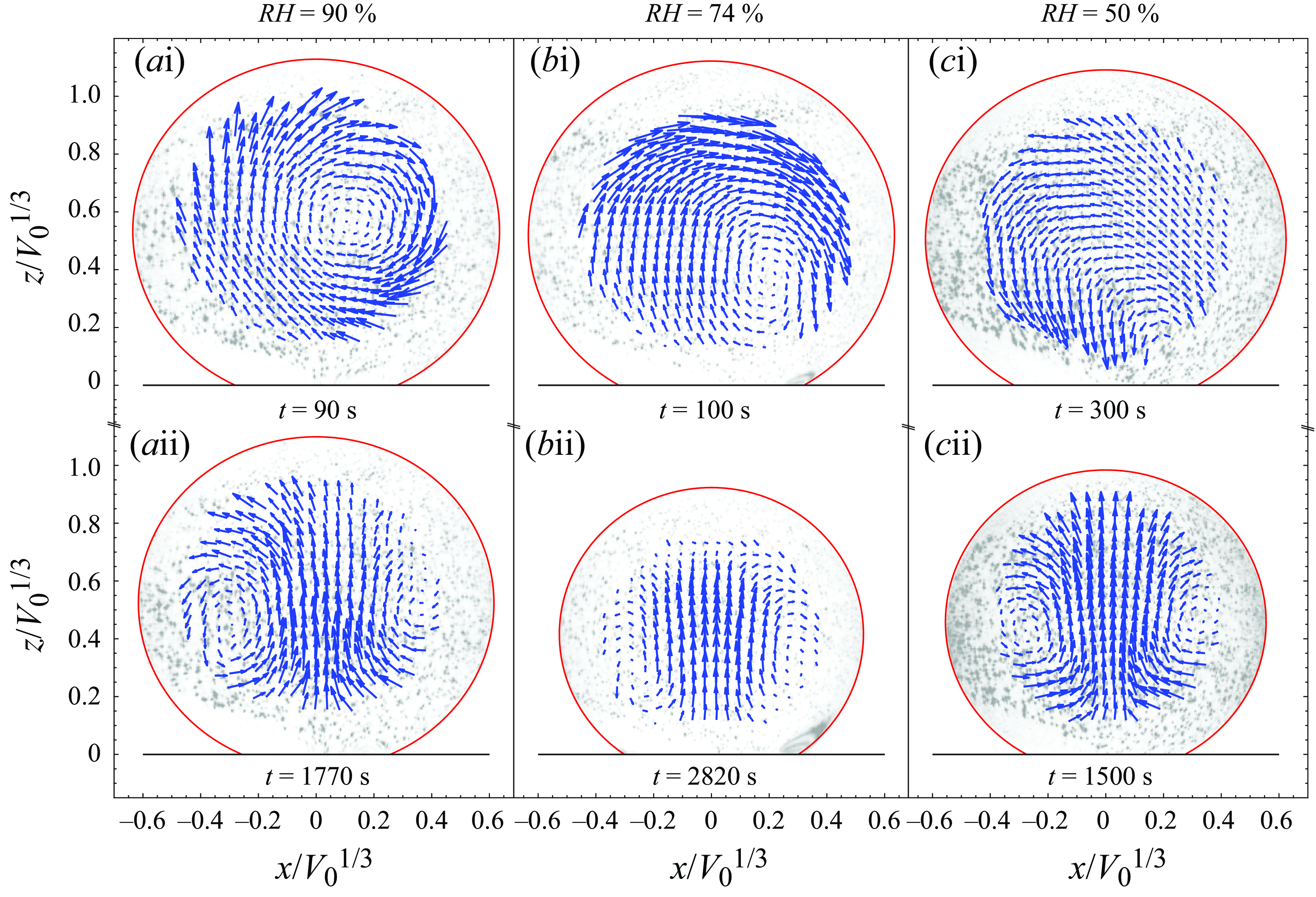
Figure 1. Experimental measurements of the flow in an evaporating drop. Each column corresponds to a measurement at a different relative humidity ( $\textit{RH}$
). The plane
$\textit{RH}$
). The plane $y=0$
is shown. The evaporation speed increases from left to right. Snapshots at two different times are shown. Initially, the flow is asymmetric, with a single roll in a different direction for each experiment (upper row). After some time, the flow becomes axisymmetric in all experiments, with a flow from the apex towards the contact line, indicating dominant thermal buoyant forces (lower row).
$y=0$
is shown. The evaporation speed increases from left to right. Snapshots at two different times are shown. Initially, the flow is asymmetric, with a single roll in a different direction for each experiment (upper row). After some time, the flow becomes axisymmetric in all experiments, with a flow from the apex towards the contact line, indicating dominant thermal buoyant forces (lower row).
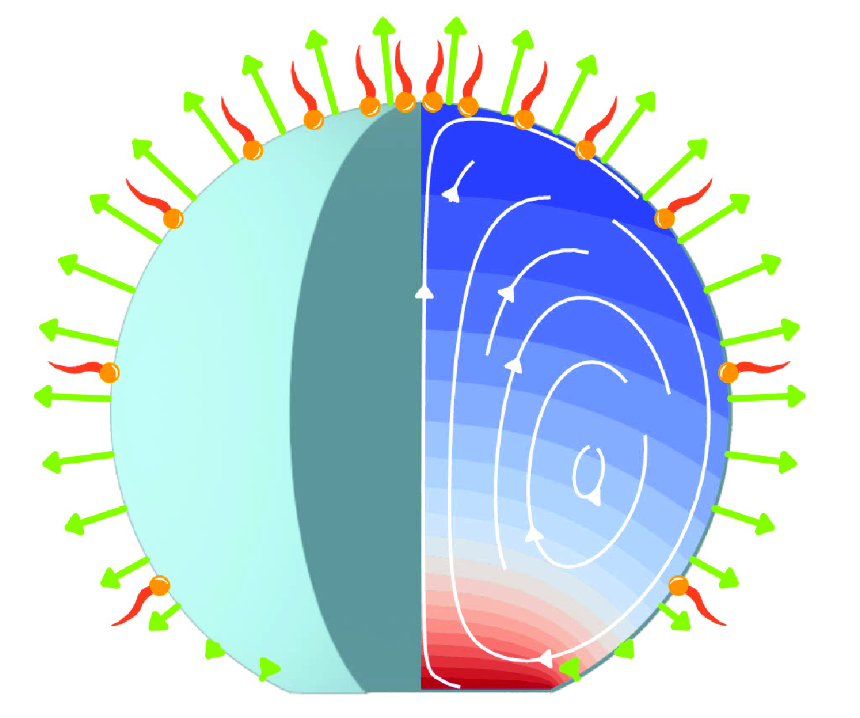
The direction of the observed axisymmetric interfacial velocity field in the late phase, from the apex towards the contact line, and directed upwards at the symmetry axis, suggests that the flow is driven by a thermal buoyant circulation (from here on, axisymmetric Rayleigh flow), and not a thermally driven Marangoni flow (from here on, axisymmetric Marangoni flow).
However, such a flow pattern transition is not always observed, even though the experiments are run under identical experimental conditions. The flow transition illustrated in figure 1 occurs in 40 % of the experiments done (a total of 50 experiments), and an additional 43 % of the experiments show either only a single-roll flow pattern or only the axisymmetric Rayleigh flow, with no observable transition. A minority of them (4 %) showed an inverted transition, from axisymmetric Rayleigh flow to single roll. Finally, a small but not negligible fraction of the experiments (13 %) showed a transition from an axisymmetric Marangoni flow, characterised by a downward-directed flow in the symmetry axis, into an axisymmetric Rayleigh flow, characterised by upward-directed flow. The variety of observed flow patterns reveals the high sensitivity of the transition due to the presence of contaminants in the environment. Despite the diversity of flow patterns observed, the most frequently observed flow patterns are clearly dominated by thermally driven convective flows, such as those shown in figure 1.
Such experimental results contrast with the theoretical predictions (Hu & Larson Reference Hu and Larson2005; Sáenz et al. Reference Sáenz, Sefiane, Kim, Matar and Valluri2015; Diddens et al. Reference Diddens, Tan, Lv, Versluis, Kuerten, Zhang and Lohse2017b ) that suggest that thermal Marangoni flows should be dominant, manifesting interfacial flows directed from the contact line towards the apex, and downward-directed flow in the symmetry axis.
This feature resembles the case of sessile droplets with lower contact angles, in which thermally driven Marangoni flows are expected to develop flow patterns even stronger than the capillary flows. However, in practice, such thermally driven flows are rather weak and only inconsistently observed (Hu & Larson Reference Hu and Larson2005; Gelderblom et al. Reference Gelderblom, Diddens and Marin2022). The most accepted explanation of this surprising feature is that the presence of contaminants at the surface hinders the thermally driven surface tension gradient at the interface.
Similarly, we hypothesise that the presence of contaminants at large contact angles is the cause of the dominance of convective flows, in the same way that capillary flows dominate the evaporation-driven flows in low contact angle sessile droplets (Deegan et al. Reference Deegan, Bakajin, Dupont, Huber, Nagel and Witten1997; Gelderblom et al. Reference Gelderblom, Diddens and Marin2022). The presence of contaminants also explains the large diversity of flow patterns observed in our experimental results. In the experiments of figure 1, the time of the transition from single roll to axisymmetric Rayleigh flow is significantly different. We theorise that this is due mainly to different amounts of contaminants being present. Experimentally, we have not observed a strong dependence of the flow pattern on the relative humidity.
In the remainder of the paper, we explore the influence of the presence of contaminants at the droplet’s interface by making use of numerical methods, as has been done in previous studies (Savino et al. Reference Savino, Paterna and Favaloro2002; Hu & Larson Reference Hu and Larson2005, Reference Hu and Larson2006; Xu & Luo Reference Xu and Luo2007; Girard et al. Reference Girard, Antoni and Sefiane2008; van Gaalen et al. Reference van Gaalen, Wijshoff, Kuerten and Diddens2022).
3. Numerical models: governing equations
3.1. Transient model
We consider a simple model that captures the essential physics of the experiments. A similar model has been used by Diddens et al. (Reference Diddens, Li and Lohse2021) for the prediction of the flow inside an evaporating binary glycerol–water droplet. Here, however, the temperature field inside a pure water droplet is considered, rather than the compositional change of the species.
A droplet of initial volume $V_0$
, density
$V_0$
, density $\rho$
, viscosity
$\rho$
, viscosity $\mu$
, thermal conductivity
$\mu$
, thermal conductivity $k$
and specific heat capacity
$k$
and specific heat capacity $c_p$
is deposited on a substrate, forming a contact angle
$c_p$
is deposited on a substrate, forming a contact angle $\theta$
; see figure 2. The substrate is approximated to be perfectly thermally conductive, such that its temperature is set to the ambient temperature
$\theta$
; see figure 2. The substrate is approximated to be perfectly thermally conductive, such that its temperature is set to the ambient temperature $T_0$
, which is far below the boiling point. Considering finite thermal conductibility would result in lower thermal gradients within the droplet, weakening the thermal Marangoni effects. However, our numerical tests with the experimental thermal conductibility of the substrate suggest that the interfacial velocity remains of the same order of magnitude as by considering a perfectly thermally conductive substrate, thereby justifying neglecting this effect. The droplet is surrounded by air at
$T_0$
, which is far below the boiling point. Considering finite thermal conductibility would result in lower thermal gradients within the droplet, weakening the thermal Marangoni effects. However, our numerical tests with the experimental thermal conductibility of the substrate suggest that the interfacial velocity remains of the same order of magnitude as by considering a perfectly thermally conductive substrate, thereby justifying neglecting this effect. The droplet is surrounded by air at $T_0$
and relative humidity
$T_0$
and relative humidity $RH = c_{\infty }/c_{{sat}}$
, where
$RH = c_{\infty }/c_{{sat}}$
, where $c_\infty$
is the vapour concentration far from the droplet, and
$c_\infty$
is the vapour concentration far from the droplet, and $c_{{sat}}$
is the vapour saturation concentration at atmospheric pressure and constant
$c_{{sat}}$
is the vapour saturation concentration at atmospheric pressure and constant $T_0$
. All liquid properties are temperature-dependent.
$T_0$
. All liquid properties are temperature-dependent.
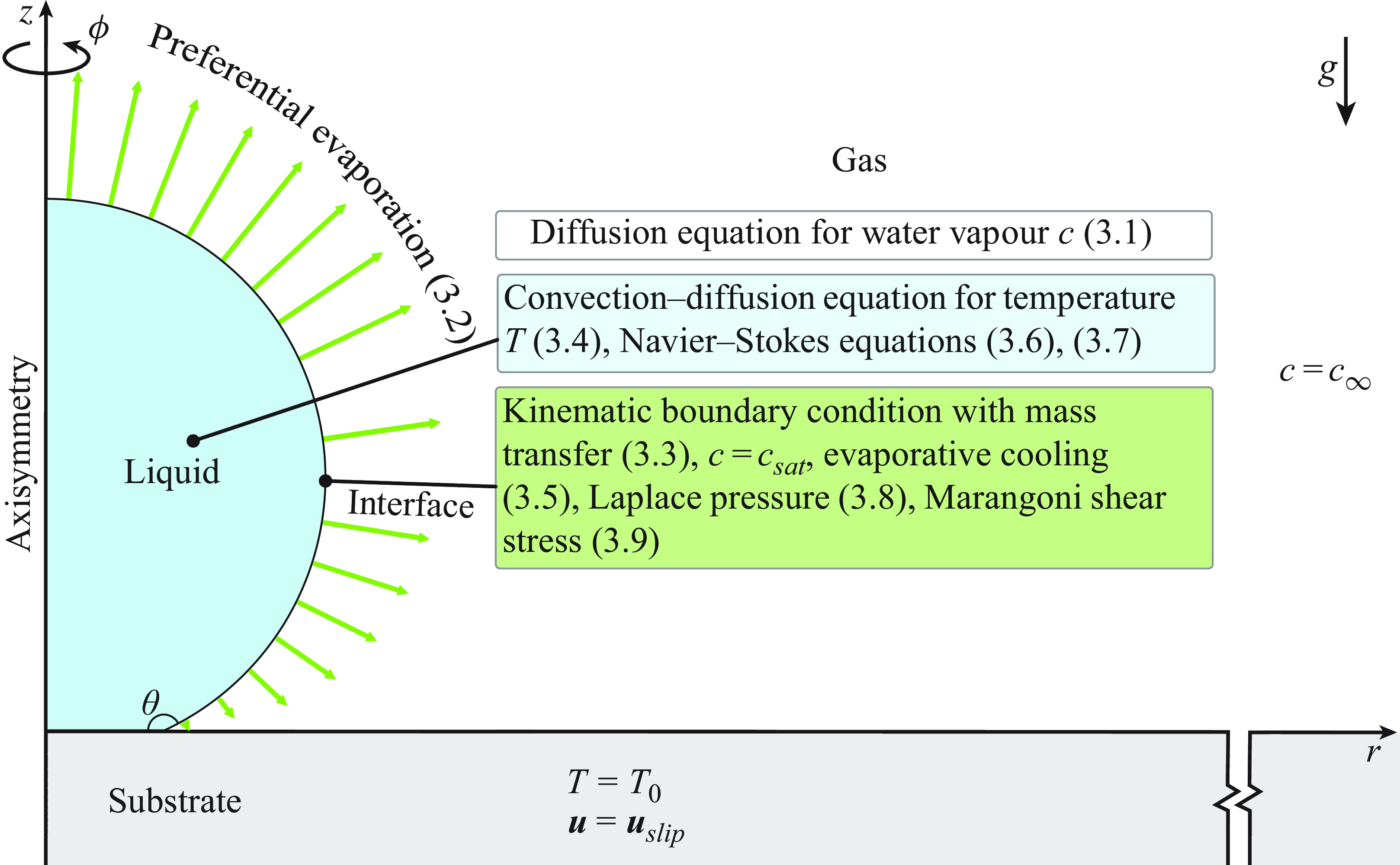
Figure 2. Schematics of the model used in the numerical simulations.
We consider the gas surrounding the water to be in a quiescent state. The solutal and thermal Rayleigh numbers of the water vapour around the droplet are defined as (Dietrich et al. Reference Dietrich, Wildeman, Visser, Hofhuis, Kooij, Zandvliet and Lohse2016) ${Ra}_c^g = (\beta _c^g g V)/(\mu ^g \kappa _c^g)$
and
${Ra}_c^g = (\beta _c^g g V)/(\mu ^g \kappa _c^g)$
and ${Ra}_T^g = (\beta _T^g g V)/(\mu ^g \kappa _T^g)$
, respectively. Here,
${Ra}_T^g = (\beta _T^g g V)/(\mu ^g \kappa _T^g)$
, respectively. Here, $\beta _c^g = (\partial \rho ^g / \partial c)/\rho ^g$
is the solutal expansion coefficient,
$\beta _c^g = (\partial \rho ^g / \partial c)/\rho ^g$
is the solutal expansion coefficient, $\rho ^g$
is the gas density,
$\rho ^g$
is the gas density, $c$
is the gas vapour concentration,
$c$
is the gas vapour concentration, $g$
is gravitational force,
$g$
is gravitational force, $\mu ^g$
is the dynamic viscosity of the gas,
$\mu ^g$
is the dynamic viscosity of the gas, $\kappa _c^g$
is the diffusivity of the solutal vapour,
$\kappa _c^g$
is the diffusivity of the solutal vapour, $\beta _T^g = (\partial \rho ^g / \partial T)/\rho ^g$
is the thermal expansion coefficient, and
$\beta _T^g = (\partial \rho ^g / \partial T)/\rho ^g$
is the thermal expansion coefficient, and $\kappa _c^g$
is the diffusivity of the thermal vapour. When calculating
$\kappa _c^g$
is the diffusivity of the thermal vapour. When calculating ${Ra}_c$
and
${Ra}_c$
and ${Ra}_T$
for the gas and vapour around the droplet, we obtain
${Ra}_T$
for the gas and vapour around the droplet, we obtain ${Ra}_s = 1.2$
and
${Ra}_s = 1.2$
and ${Ra}_T = 0.5$
, both much smaller than the critical Rayleigh value 12 for convective effects to become relevant. Since there are no external heat sources, the water vapour concentration
${Ra}_T = 0.5$
, both much smaller than the critical Rayleigh value 12 for convective effects to become relevant. Since there are no external heat sources, the water vapour concentration $c$
can be considered to quasi-stationarily diffuse far from the droplet (see (3.1)) and the evaporation rate
$c$
can be considered to quasi-stationarily diffuse far from the droplet (see (3.1)) and the evaporation rate $j$
is given by the diffusive flux at the liquid–gas interface (see (3.2)) (Deegan et al. Reference Deegan, Bakajin, Dupont, Huber, Nagel and Witten1997, Reference Deegan, Bakajin, Dupont, Huber, Nagel and Witten2000; Deegan Reference Deegan2000; Popov Reference Popov2005):
$j$
is given by the diffusive flux at the liquid–gas interface (see (3.2)) (Deegan et al. Reference Deegan, Bakajin, Dupont, Huber, Nagel and Witten1997, Reference Deegan, Bakajin, Dupont, Huber, Nagel and Witten2000; Deegan Reference Deegan2000; Popov Reference Popov2005):
 \begin{align}&\qquad \nabla ^2 c = 0 , \end{align}
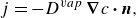 \begin{align}& j = - D^{{vap}}\, \boldsymbol \nabla c \boldsymbol \cdot \boldsymbol{n} , \end{align}
where $D^{{vap}}$
is the vapour diffusion coefficient, and
$D^{{vap}}$
is the vapour diffusion coefficient, and $\boldsymbol{n}$
is the normal to the interface. As the droplet evaporates, the droplet–gas interface moves according to the kinematic boundary condition
$\boldsymbol{n}$
is the normal to the interface. As the droplet evaporates, the droplet–gas interface moves according to the kinematic boundary condition
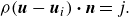 \begin{equation} \rho (\boldsymbol{u} - \boldsymbol{u}_{{i}}) \boldsymbol \cdot \boldsymbol{n} = j. \end{equation}
Here, $\boldsymbol{u}$
is the velocity field, and
$\boldsymbol{u}$
is the velocity field, and $\boldsymbol{u}_{{i}}$
is the velocity of the interface. On account of the latent heat of evaporation
$\boldsymbol{u}_{{i}}$
is the velocity of the interface. On account of the latent heat of evaporation $\Lambda$
, evaporative cooling occurs. Due to the presence of the isothermal substrate and the spatially non-uniform evaporation rate, temperature gradients along the interface are expected. In the liquid phase, if convective motion is initiated through e.g. thermal Marangoni forces, then it is expected to have significant effects on the droplet temperature profile due to the low thermal diffusivity
$\Lambda$
, evaporative cooling occurs. Due to the presence of the isothermal substrate and the spatially non-uniform evaporation rate, temperature gradients along the interface are expected. In the liquid phase, if convective motion is initiated through e.g. thermal Marangoni forces, then it is expected to have significant effects on the droplet temperature profile due to the low thermal diffusivity $\kappa = k/(\rho c_p)$
of water (or any similar liquid), which is of order
$\kappa = k/(\rho c_p)$
of water (or any similar liquid), which is of order $\kappa \sim$ ${10^{-7}}\ {\textrm m^2\ \textrm s^{-1}}$
. Therefore, we consider a convection–diffusion equation for the temperature
${10^{-7}}\ {\textrm m^2\ \textrm s^{-1}}$
. Therefore, we consider a convection–diffusion equation for the temperature $T$
in the liquid phase,
$T$
in the liquid phase,
 \begin{equation} \rho c_p ( \partial _t T + \boldsymbol{u} \boldsymbol\cdot \boldsymbol \nabla T ) = k\, \nabla ^2 T , \end{equation}
with a boundary condition for the evaporative cooling in a frame co-moving with the interface,
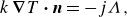 \begin{equation} k\, \boldsymbol \nabla T \boldsymbol \cdot \boldsymbol{n} = - j \Lambda , \end{equation}
and $T=T_0$
at the substrate. Thermal transport in the gas phase is disregarded due to its small contribution in the droplet’s flow features.
$T=T_0$
at the substrate. Thermal transport in the gas phase is disregarded due to its small contribution in the droplet’s flow features.
We consider the $z$
-axis to be the vertical axis pointing to the apex of the droplet, and gravity
$z$
-axis to be the vertical axis pointing to the apex of the droplet, and gravity $g$
acts in the negative
$g$
acts in the negative $z$
-direction for a sessile droplet, a configuration to which this study is restricted. The velocity field and pressure
$z$
-direction for a sessile droplet, a configuration to which this study is restricted. The velocity field and pressure $p$
are governed by the Navier–Stokes equation
$p$
are governed by the Navier–Stokes equation
 \begin{equation} \rho ( \partial _t \boldsymbol{u}+ \boldsymbol{u} \boldsymbol \cdot \boldsymbol \nabla \boldsymbol{u} ) = - \boldsymbol \nabla p + \mu\, \nabla ^2 \boldsymbol{u} + \rho \boldsymbol{g}, \end{equation}
where $\boldsymbol{g} = - g \boldsymbol{e}_z$
is the gravitational acceleration (
$\boldsymbol{g} = - g \boldsymbol{e}_z$
is the gravitational acceleration ( $\boldsymbol{e}_z$
is the unit vector in the
$\boldsymbol{e}_z$
is the unit vector in the $z$
-direction, positive upwards). The mass conservation is ensured by the continuity equation
$z$
-direction, positive upwards). The mass conservation is ensured by the continuity equation
 \begin{equation} \partial _t \rho + \boldsymbol \nabla \boldsymbol \cdot (\rho \boldsymbol{u})=0 . \end{equation}
Similarly to what is considered by Diddens et al. (Reference Diddens, Li and Lohse2021), we take a small slip length to simulate the assumed pinned contact line in Constant Contact Radius mode (Picknett & Bexon Reference Picknett and Bexon1977) to resolve the incompatibility of no-slip at the substrate and evaporation at the contact line. As long as the slip length is orders of magnitude smaller than the droplet size, the results are independent of the slip length (Diddens et al. Reference Diddens, Li and Lohse2021), which is also confirmed by our simulations.
The liquid–gas interface must account for the Laplace pressure and Marangoni stresses, which are given by
 \begin{equation} \boldsymbol{n} \boldsymbol \cdot ( - p \boldsymbol{I} + \mu (\boldsymbol \nabla \boldsymbol{u} + (\boldsymbol \nabla \boldsymbol{u})^{\textrm T}) ) \boldsymbol \cdot \boldsymbol{n} = \sigma C \boldsymbol{n} \end{equation}
and
 \begin{equation} \boldsymbol{n} \boldsymbol \cdot (\mu (\boldsymbol \nabla \boldsymbol{u} + (\boldsymbol \nabla \boldsymbol{u})^{\textrm T}) ) \boldsymbol \cdot \boldsymbol{t} = \boldsymbol \nabla _t \sigma \boldsymbol \cdot \boldsymbol{t} \, . \end{equation}
Here, $\boldsymbol{t}$
is the tangential vector to the interface,
$\boldsymbol{t}$
is the tangential vector to the interface, $\boldsymbol{I}$
is the identity matrix,
$\boldsymbol{I}$
is the identity matrix, $C$
is the curvature of the interface, and
$C$
is the curvature of the interface, and $\boldsymbol \nabla _t$
is the surface derivative at the interface.
$\boldsymbol \nabla _t$
is the surface derivative at the interface.
3.2. Quasi-stationary model
In a droplet evaporating at ambient conditions, the velocity $\boldsymbol{u}$
associated with the circulation within the droplet is typically much faster than the velocity of the interface
$\boldsymbol{u}$
associated with the circulation within the droplet is typically much faster than the velocity of the interface $\boldsymbol{u}_{{i}}$
(Diddens et al. Reference Diddens, Tan, Lv, Versluis, Kuerten, Zhang and Lohse2017b
). Buoyancy and thermal Marangoni forces form a quasi-equilibrium, thereby justifying the quasi-stationary approximation. The kinematic boundary condition (3.3) is then reduced to
$\boldsymbol{u}_{{i}}$
(Diddens et al. Reference Diddens, Tan, Lv, Versluis, Kuerten, Zhang and Lohse2017b
). Buoyancy and thermal Marangoni forces form a quasi-equilibrium, thereby justifying the quasi-stationary approximation. The kinematic boundary condition (3.3) is then reduced to $\boldsymbol{u} \boldsymbol{\cdot} \boldsymbol{n} = 0$
, which can be imposed numerically via a Lagrange multiplier field at the interface. Due to its small size, the temperature variations within the droplet are typically a few per cent of the absolute ambient temperature. It is then reasonable to consider an expansion of the temperature into
$\boldsymbol{u} \boldsymbol{\cdot} \boldsymbol{n} = 0$
, which can be imposed numerically via a Lagrange multiplier field at the interface. Due to its small size, the temperature variations within the droplet are typically a few per cent of the absolute ambient temperature. It is then reasonable to consider an expansion of the temperature into $ T(\boldsymbol{x},t) = T_0 + \Delta T(\boldsymbol{x},t)$
, i.e. the ambient temperature summed with the small local variations
$ T(\boldsymbol{x},t) = T_0 + \Delta T(\boldsymbol{x},t)$
, i.e. the ambient temperature summed with the small local variations $\Delta T(\boldsymbol{x},t)$
. Taking these approximations, it is logical to expand the density and surface tension into first-order Taylor series around the ambient temperature
$\Delta T(\boldsymbol{x},t)$
. Taking these approximations, it is logical to expand the density and surface tension into first-order Taylor series around the ambient temperature $T_0$
:
$T_0$
:
 \begin{align} \rho (T) &= \rho _0 + (T - T_0)\, \left . {\partial _T \rho } \right |_{T_0} , \end{align}
 \begin{align} \sigma (T) &= \sigma _0 + (T - T_0)\, \left . {\partial _T \sigma } \right |_{T_0} , \end{align}
where $\rho _0$
and
$\rho _0$
and $\sigma _0$
are the density and surface tension at
$\sigma _0$
are the density and surface tension at $T_0$
, and
$T_0$
, and $\left . {\partial _T \rho } \right |_{T_0}$
and
$\left . {\partial _T \rho } \right |_{T_0}$
and $\left . {\partial _T \sigma } \right |_{T_0}$
are the first-order derivatives of the density and surface tension with respect to the temperature, evaluated at
$\left . {\partial _T \sigma } \right |_{T_0}$
are the first-order derivatives of the density and surface tension with respect to the temperature, evaluated at $T_0$
. We simplify the notation to
$T_0$
. We simplify the notation to $\partial _T \rho$
and
$\partial _T \rho$
and $\partial _T \sigma$
in the following. All other properties are considered to be constant and are evaluated at
$\partial _T \sigma$
in the following. All other properties are considered to be constant and are evaluated at $T_0$
, i.e.
$T_0$
, i.e. $\mu =\mu _0$
,
$\mu =\mu _0$
, $k=k_0$
,
$k=k_0$
, $c_p=c_{p0}$
,
$c_p=c_{p0}$
, $D^{{vap}}=D^{{vap}}_0$
,
$D^{{vap}}=D^{{vap}}_0$
, $\Lambda = \Lambda _0$
,
$\Lambda = \Lambda _0$
, $c_{{sat}}=c_{{sat0}}$
– that is, we assume the Oberbeck–Boussinesq approximation for these properties.
$c_{{sat}}=c_{{sat0}}$
– that is, we assume the Oberbeck–Boussinesq approximation for these properties.
We scale the vapour concentration such that $\tilde {c}=1$
at the droplet–gas interface, and
$\tilde {c}=1$
at the droplet–gas interface, and $\tilde {c}=0$
far away. For the temperature differences
$\tilde {c}=0$
far away. For the temperature differences $T-T_0$
, one should take into consideration that no temperature difference should be expected when no evaporation happens, i.e. when relative humidity is 100 % (or
$T-T_0$
, one should take into consideration that no temperature difference should be expected when no evaporation happens, i.e. when relative humidity is 100 % (or $c_{{sat}}=c_\infty$
). We choose the factors in evaporative cooling (3.5) for the scaling of the temperature variation:
$c_{{sat}}=c_\infty$
). We choose the factors in evaporative cooling (3.5) for the scaling of the temperature variation:
 \begin{equation} \begin{aligned} (c-c_\infty ) &= (c_{{sat}}-c_\infty )\tilde {c} , \quad (T-T_0) = \dfrac {(c_{{sat}}-c_\infty ) \Lambda _0 D^{{vap}}_0}{k_0} \tilde {T} . \end{aligned} \end{equation}
We take the cubic root of the volume to non-dimensionalise length scales. The thermal diffusivity $\kappa _0 = k_0/(\rho _0 c_{p0})$
is taken to non-dimensionalise time, since thermal effects dictate the flow. We then have
$\kappa _0 = k_0/(\rho _0 c_{p0})$
is taken to non-dimensionalise time, since thermal effects dictate the flow. We then have
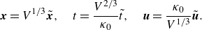 \begin{equation} \begin{aligned} \boldsymbol{x} = V^{1/3} \tilde {\boldsymbol{x}}, \quad t = \frac {V^{2/3}}{\kappa _0} \tilde {t} , \quad \boldsymbol{u}= \frac {\kappa _0}{V^{1/3}} \tilde {\boldsymbol{u}}. \end{aligned} \end{equation}
A dimensionless mass transfer rate $\tilde {j}$
can then be defined as
$\tilde {j}$
can then be defined as $\tilde {j} = V^{1/3}/(D^{vap}_0 (c_{sat}-c_\infty )) j = \boldsymbol \nabla \tilde {c} \boldsymbol \cdot \boldsymbol{n}$
. In non-dimensional form, (3.4) and (3.5) can be rewritten as
$\tilde {j} = V^{1/3}/(D^{vap}_0 (c_{sat}-c_\infty )) j = \boldsymbol \nabla \tilde {c} \boldsymbol \cdot \boldsymbol{n}$
. In non-dimensional form, (3.4) and (3.5) can be rewritten as
 \begin{align}& \partial _{\tilde {t}} \tilde {T} + \tilde {\boldsymbol{u}} \boldsymbol \cdot \tilde {\boldsymbol \nabla } \tilde {T} = \tilde {\nabla }^2 \tilde {T} , \end{align}
 \begin{align}&\qquad \tilde {\boldsymbol \nabla } \tilde {T} \boldsymbol \cdot \boldsymbol{n} = - \tilde {j} . \end{align}
The Oberbeck–Boussinesq approximation is taken for the Navier–Stokes equations since $(T-T_0)\, \partial _T \rho$
is small compared to
$(T-T_0)\, \partial _T \rho$
is small compared to $\rho _0$
. The density appears as in (3.10) only in the gravity term
$\rho _0$
. The density appears as in (3.10) only in the gravity term $\rho \boldsymbol{g}$
, while considered constant
$\rho \boldsymbol{g}$
, while considered constant $\rho _0$
in the remaining terms. Due to the small Reynolds number (
$\rho _0$
in the remaining terms. Due to the small Reynolds number ( $\sim 0.1$
at experimental conditions), Stokes flow is assumed to be sufficient. Equations (3.6) and (3.7) can then be reduced to
$\sim 0.1$
at experimental conditions), Stokes flow is assumed to be sufficient. Equations (3.6) and (3.7) can then be reduced to
 \begin{align}&\qquad\qquad\quad \tilde {\boldsymbol \nabla } \boldsymbol \cdot \tilde {\boldsymbol{u}} = 0 , \end{align}
 \begin{align}& - \tilde {\boldsymbol \nabla } \tilde {p} + \tilde {\nabla }^2\boldsymbol{u} + {Ra}_T\, \tilde {T} \boldsymbol{e}_z = 0, \end{align}
where
 \begin{equation} \tilde {p} = \frac {V^{2/3}}{\kappa _0 \mu _0} (p - \rho _0 g z) \, \end{equation}
is the non-dimensional pressure, and
 \begin{equation} {Ra}_T = \frac {V g\, |\partial _{\tilde T} \rho |}{\kappa _0 \mu _0} \end{equation}
is the thermal Rayleigh number.
To remove the null space of the pressure field, we use a Lagrange multiplier, which ensures that the average pressure $\tilde {p}$
in the liquid domain is zero. Note that we derive
$\tilde {p}$
in the liquid domain is zero. Note that we derive $\rho$
with the non-dimensional temperature
$\rho$
with the non-dimensional temperature $\tilde T$
to ensure that
$\tilde T$
to ensure that $RaT=0$
in the absence of evaporation, e.g. when
$RaT=0$
in the absence of evaporation, e.g. when $c_{{sat}}=c_\infty$
. The non-dimensional capillary (3.8) and Marangoni (3.9) forces are given by
$c_{{sat}}=c_\infty$
. The non-dimensional capillary (3.8) and Marangoni (3.9) forces are given by
 \begin{align}& \tilde {p} + \boldsymbol{n} \boldsymbol \cdot (\tilde {\boldsymbol \nabla } \tilde {\boldsymbol{u}} + (\tilde {\boldsymbol \nabla } \tilde {\boldsymbol{u}})^{\textrm T}) \boldsymbol \cdot \boldsymbol{n} = \frac {1}{Ca} (\tilde {C} + Bo\, \tilde {z}) , \end{align}
 \begin{align}&\quad \boldsymbol{n} \boldsymbol \cdot (\tilde {\boldsymbol \nabla } \tilde {\boldsymbol{u}} + (\tilde {\boldsymbol \nabla } \tilde {\boldsymbol{u}})^{\textrm T}) \boldsymbol \cdot \boldsymbol{t} = - {Ma}_T\, \tilde {\boldsymbol \nabla }_t \tilde {T} \boldsymbol{\cdot} \boldsymbol{t} , \end{align}
where the capillary number $Ca$
, the Bond number
$Ca$
, the Bond number $Bo$
and the thermal Marangoni number
$Bo$
and the thermal Marangoni number ${Ma}_T$
are given by
${Ma}_T$
are given by
 \begin{equation} \begin{aligned} Ca = \frac {\kappa _0 \mu _0}{V^{1/3} \sigma _0}, \quad Bo = \frac {\rho _0 g V^{2/3}}{\sigma _0} , \quad {Ma}_T = \frac {V^{1/3} \,|\partial _{\tilde T} \sigma |}{\kappa _0 \mu _0} . \end{aligned} \end{equation}
In small droplets, the capillary number is small ( ${\sim}10^{-6}$
at the experimental conditions). Since the Bond number is also small (
${\sim}10^{-6}$
at the experimental conditions). Since the Bond number is also small ( ${\sim}10^{-1}$
at the experimental conditions), the last term of (3.20) is assumed to be irrelevant, leading to an equilibrium spherical-cap shape with a constant contact angle
${\sim}10^{-1}$
at the experimental conditions), the last term of (3.20) is assumed to be irrelevant, leading to an equilibrium spherical-cap shape with a constant contact angle $\theta$
.
$\theta$
.
In our model, we have considered only the case of decreasing density and surface tension with increasing temperature, which is the case for water at ambient lab conditions. This allows us to consider only positive ${Ra}_T$
and
${Ra}_T$
and ${Ma}_T$
values, following the sign convection in the definition of the system of equations.
${Ma}_T$
values, following the sign convection in the definition of the system of equations.
3.3. Procedure
The system of equations of §§ 3.1 and 3.2 are solved using a finite element method on triangular elements with the package pyoomph (https://pyoomph.github.io/) (Diddens & Rocha Reference Diddens and Rocha2024), which is based on oomph-lib (Heil & Hazel Reference Heil and Hazel2006) and GiNaC (Bauer et al., Reference Bauer, Frink and Kreckel2002). The code was mutually validated by an analogous implementation in ngsolve (Schöberl Reference Schöberl1997). The mesh motion in the transient model of § 3.1 is modelled by using an arbitrary Lagrangian–Eulerian method. Since the droplet geometry is assumed to be axially symmetric, a two-dimensional mesh is used in all simulations, even when analysing the azimuthal symmetry-breaking phenomenon (§ 4.3). This can be done by assuming that the axial symmetry is broken in a bifurcation, due to instabilities that act on an azimuthal wavenumber $m$
. We employ the method described and validated by Diddens & Rocha (Reference Diddens and Rocha2024), a linear stability analysis method that allows investigation of symmetry-breaking instabilities. Together with bifurcation tracking and pseudo-arc-length continuation methods, this tool allows identification of the critical parameters for which the symmetry is broken.
$m$
. We employ the method described and validated by Diddens & Rocha (Reference Diddens and Rocha2024), a linear stability analysis method that allows investigation of symmetry-breaking instabilities. Together with bifurcation tracking and pseudo-arc-length continuation methods, this tool allows identification of the critical parameters for which the symmetry is broken.
The vapour diffusion equation (3.1) in the gas phase is discretised using first-order continuous Lagrangian elements. Its solution then provides the value of the evaporation rate $\tilde {j}$
at the interface. In order to spatially approximate the velocity–pressure pair in the Stokes equation, MINI-elements (Arnold, Brezzi & Fortin Reference Arnold, Brezzi and Fortin1984) are used. The temperature field is approximated using first-order continuous Lagrangian elements. The choices of the latter two spaces are made in order to avoid spurious oscillations in the tangential velocity at the droplet–gas interface. Further details concerning the choice of field spaces are provided in Appendix A.
$\tilde {j}$
at the interface. In order to spatially approximate the velocity–pressure pair in the Stokes equation, MINI-elements (Arnold, Brezzi & Fortin Reference Arnold, Brezzi and Fortin1984) are used. The temperature field is approximated using first-order continuous Lagrangian elements. The choices of the latter two spaces are made in order to avoid spurious oscillations in the tangential velocity at the droplet–gas interface. Further details concerning the choice of field spaces are provided in Appendix A.
In § 4.2, we calculate the percentage of the total volume of liquid associated with the stream function $\psi$
that flows in the direction from the apex towards the contact line. This percentage is denoted as
$\psi$
that flows in the direction from the apex towards the contact line. This percentage is denoted as $\psi ^+$
. The value of
$\psi ^+$
. The value of $\psi ^+$
provides insight into the dominant forces driving the flow. Specifically, if
$\psi ^+$
provides insight into the dominant forces driving the flow. Specifically, if $\psi ^+ \gt 90\,\%$
, then the flow is considered to be dominated by buoyancy forces, and if
$\psi ^+ \gt 90\,\%$
, then the flow is considered to be dominated by buoyancy forces, and if $\psi ^+ \lt 10\,\%$
, then the flow is considered to be dominated by thermocapillary forces. By fixing
$\psi ^+ \lt 10\,\%$
, then the flow is considered to be dominated by thermocapillary forces. By fixing ${Ma}_T$
, we can formally consider
${Ma}_T$
, we can formally consider ${Ra}_T$
as a Lagrange multiplier to obtain the unique
${Ra}_T$
as a Lagrange multiplier to obtain the unique ${Ra}_T$
value that satisfies each
${Ra}_T$
value that satisfies each $\psi ^+$
constraint. Subsequently, we employ pseudo-arc-length continuation to trace the curves that delineate the regime where there is competition between Marangoni and Rayleigh effects.
$\psi ^+$
constraint. Subsequently, we employ pseudo-arc-length continuation to trace the curves that delineate the regime where there is competition between Marangoni and Rayleigh effects.
4. Pure water droplet: numerical results
4.1. At experimental conditions: analysis of the axisymmetric flow direction
We take the initial experimental conditions of figure 1(c) as input for the numerical simulations to compare the results. More specifically, we consider here: $RH=50\,\%$
,
$RH=50\,\%$
, $T_0=21\,^\circ$
C,
$T_0=21\,^\circ$
C, $V_0={5.6}\ {\unicode{x03BC} }{\textrm l}$
and
$V_0={5.6}\ {\unicode{x03BC} }{\textrm l}$
and $\theta =150^\circ$
. The transient model of § 3.1 is used here to describe the time evolution of the evaporating droplet. The Young–Laplace equation is solved to obtain the slightly gravity-deformed droplet shape at deposition time, used as the initial geometry condition for our simulations.
$\theta =150^\circ$
. The transient model of § 3.1 is used here to describe the time evolution of the evaporating droplet. The Young–Laplace equation is solved to obtain the slightly gravity-deformed droplet shape at deposition time, used as the initial geometry condition for our simulations.
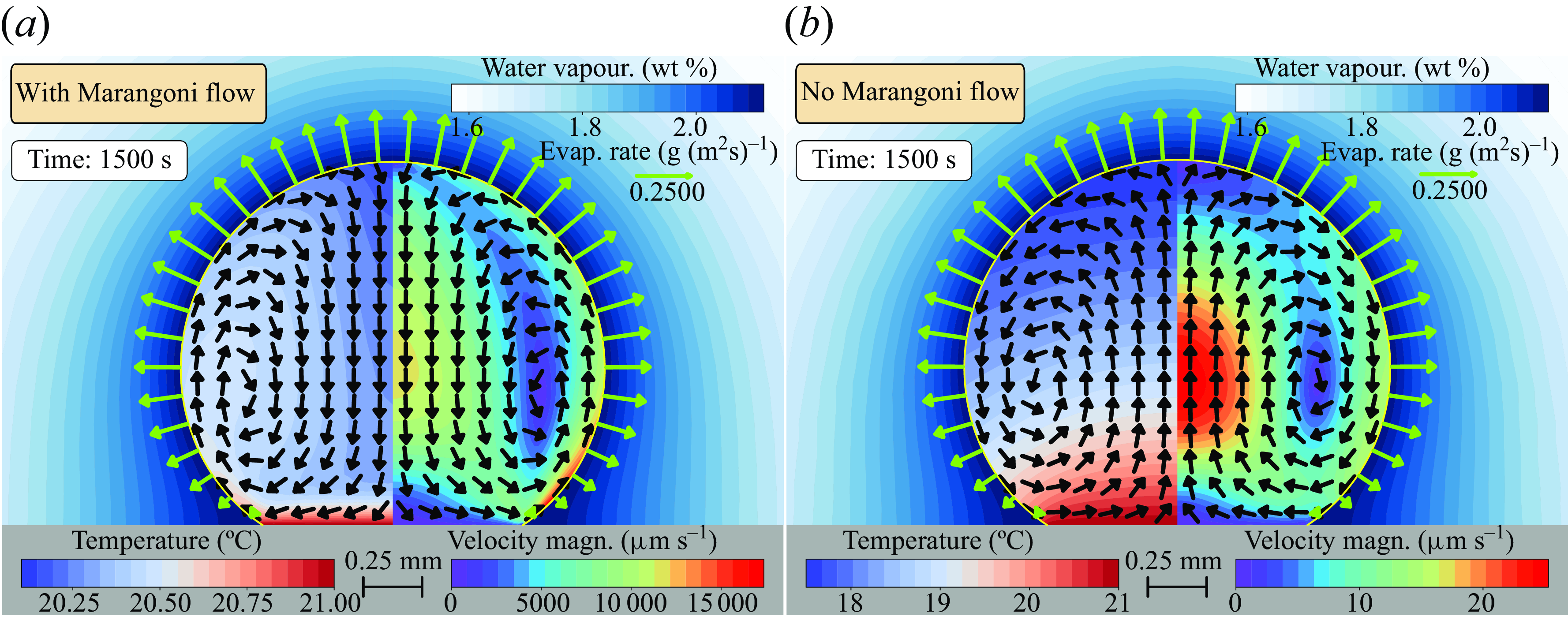
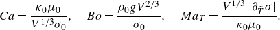
Figure 3. Numerical results for the temperature and velocity magnitude fields at the initial experimental conditions of figure 1(c), i.e. $RH=50\,\%$
,
$RH=50\,\%$
, $T_0=21^\circ$
C,
$T_0=21^\circ$
C, $V_0={5.6}\ {\unicode{x03BC} }\text{l}$
and
$V_0={5.6}\ {\unicode{x03BC} }\text{l}$
and $\theta =150^\circ$
, 1500 s after deposition on the substrate. (a) Considering all effects generating the flow, the flow direction is axisymmetric, going from the rim to the apex, indicating dominant thermocapillary forces. (b) If the surface tension is considered constant, then the flow direction of the axisymmetric flow is the other way around, namely from the apex to the rim, indicating dominance of the buoyancy forces.
$\theta =150^\circ$
, 1500 s after deposition on the substrate. (a) Considering all effects generating the flow, the flow direction is axisymmetric, going from the rim to the apex, indicating dominant thermocapillary forces. (b) If the surface tension is considered constant, then the flow direction of the axisymmetric flow is the other way around, namely from the apex to the rim, indicating dominance of the buoyancy forces.
We analyse the flow direction obtained numerically in a time frame where the experiments present an axisymmetric flow from the apex towards the contact line, in particular 1500 s after deposition, as depicted in figure 1(cii). At this instant, the numerical calculations show a vortex in the droplet from the contact line towards the apex, indicating dominant thermocapillary forces; see figure 3(a). The velocity magnitude is of the order of $\sim {10}\ {\textrm {mm s}}^{-1}$
, which is significantly larger than the experimental measurements,
$\sim {10}\ {\textrm {mm s}}^{-1}$
, which is significantly larger than the experimental measurements, $\sim {1}\ {\unicode{x03BC} }{\textrm {m}\ {\textrm s}}^{-1}$
. One can theoretically consider a constant surface tension to disregard any Marangoni flow; see figure 3(b). Here, despite the theoretical assumption, the flow direction agrees well with the experimental results, and the velocity magnitude is much closer to that of the experiments,
$\sim {1}\ {\unicode{x03BC} }{\textrm {m}\ {\textrm s}}^{-1}$
. One can theoretically consider a constant surface tension to disregard any Marangoni flow; see figure 3(b). Here, despite the theoretical assumption, the flow direction agrees well with the experimental results, and the velocity magnitude is much closer to that of the experiments, $\sim {10}\ {\unicode{x03BC} }{\textrm{m s}}^{-1}$
. The discrepancy in flow direction and velocity magnitude between the numerical and experimental results is evident, indicating that there is an additional factor that significantly reduces the thermal Marangoni forces, resulting in a thermal-buoyancy-driven flow.
$\sim {10}\ {\unicode{x03BC} }{\textrm{m s}}^{-1}$
. The discrepancy in flow direction and velocity magnitude between the numerical and experimental results is evident, indicating that there is an additional factor that significantly reduces the thermal Marangoni forces, resulting in a thermal-buoyancy-driven flow.
4.2. Phase diagram of the axisymmetric flow direction
Hereinafter, the quasi-stationary model of § 3.2 is used for the following calculations. We present a comprehensive analysis of the flow direction inside a droplet of $\theta =150^\circ$
, in a
$\theta =150^\circ$
, in a ${Ma}_T$
–
${Ma}_T$
– ${Ra}_T$
phase diagram (figure 4), assuming axial symmetry. To ensure the accuracy of our findings, we first examine the stability of the stationary solution across the entire parameter space. By calculating the eigenvalues of the linearised system of equations, we determine whether the obtained stationary solution is stable. From figure 4, one can identify a small bistable region where multiple stable solutions coexist for the same
${Ra}_T$
phase diagram (figure 4), assuming axial symmetry. To ensure the accuracy of our findings, we first examine the stability of the stationary solution across the entire parameter space. By calculating the eigenvalues of the linearised system of equations, we determine whether the obtained stationary solution is stable. From figure 4, one can identify a small bistable region where multiple stable solutions coexist for the same ${Ma}_T$
and
${Ma}_T$
and ${Ra}_T$
values. For simplicity, we exclude this region from our analysis, as indicated by the grey area in the phase diagram. Then three remaining distinct regions can be identified in the phase space: the blue region, where buoyancy forces predominantly drive the flow, corresponding to
${Ra}_T$
values. For simplicity, we exclude this region from our analysis, as indicated by the grey area in the phase diagram. Then three remaining distinct regions can be identified in the phase space: the blue region, where buoyancy forces predominantly drive the flow, corresponding to ${Ma}_T$
and
${Ma}_T$
and ${Ra}_T$
values such that
${Ra}_T$
values such that $\psi ^+ \gt 90\,\%$
; the orange region, where thermocapillary forces primarily drive the flow, bounded by the curve
$\psi ^+ \gt 90\,\%$
; the orange region, where thermocapillary forces primarily drive the flow, bounded by the curve $\psi ^+ \lt 10\,\%$
; and the yellow region, where two competing vortices are observed, defined by
$\psi ^+ \lt 10\,\%$
; and the yellow region, where two competing vortices are observed, defined by $10\,\% \leqslant \psi ^+ \leqslant 90\,\%$
.
$10\,\% \leqslant \psi ^+ \leqslant 90\,\%$
.
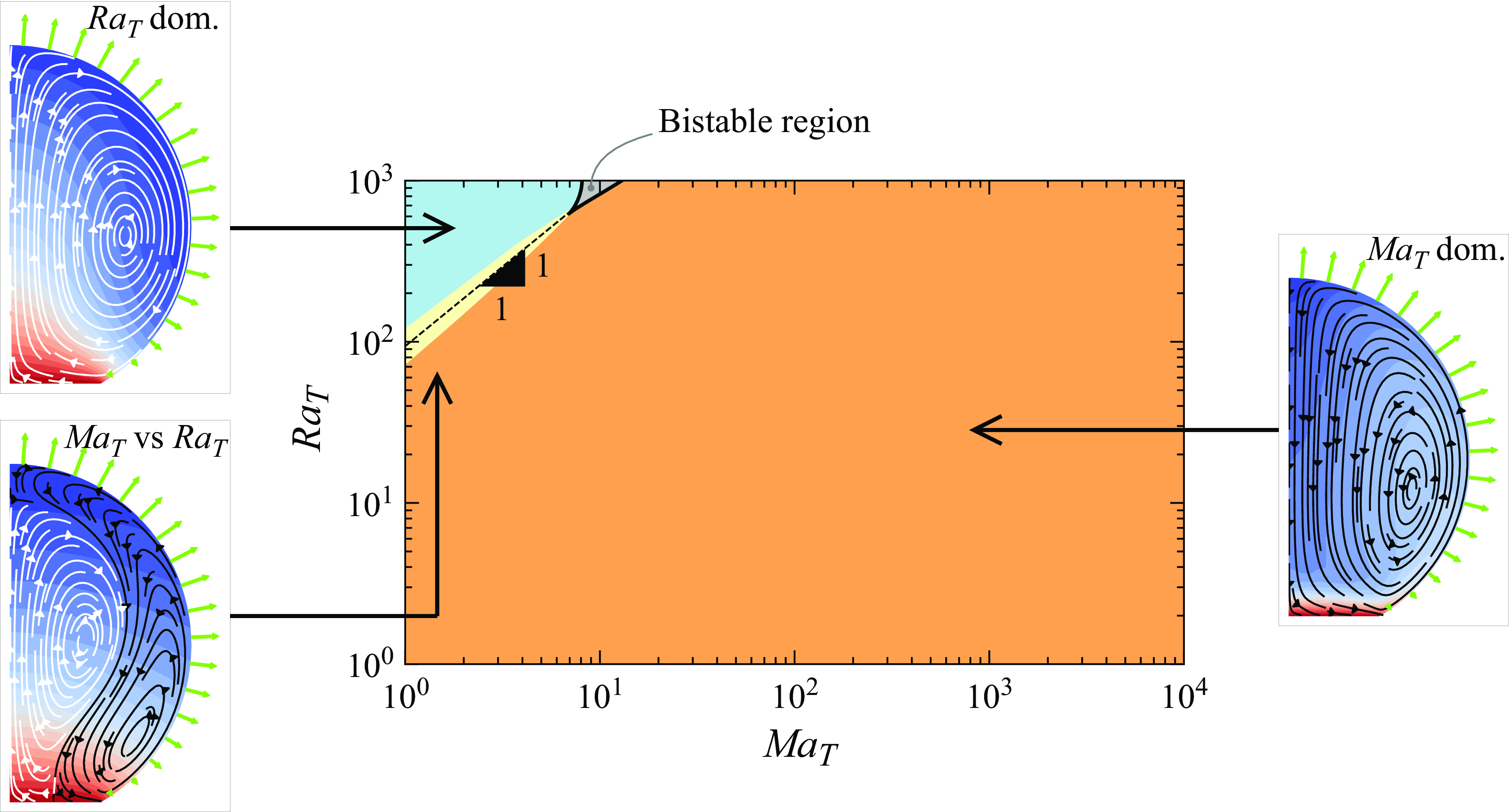
Figure 4. The ${Ma}_T$
–
${Ma}_T$
– ${Ra}_T$
phase diagram for flow direction for droplet of
${Ra}_T$
phase diagram for flow direction for droplet of $\theta =150^\circ$
. The grey area represents the bistable region, where multiple stable solutions coexist for the same
$\theta =150^\circ$
. The grey area represents the bistable region, where multiple stable solutions coexist for the same ${Ma}_T$
and
${Ma}_T$
and ${Ra}_T$
values. The blue region is dominated by thermal buoyancy, while the orange region is dominated by thermocapillary forces. In the yellow region, one observes rolls driven by both thermal Marangoni flow and thermal buoyancy. The black dashed line represents the
${Ra}_T$
values. The blue region is dominated by thermal buoyancy, while the orange region is dominated by thermocapillary forces. In the yellow region, one observes rolls driven by both thermal Marangoni flow and thermal buoyancy. The black dashed line represents the $\psi ^+=50\,\%$
curve, where the competing vortices occupy equal volumes.
$\psi ^+=50\,\%$
curve, where the competing vortices occupy equal volumes.
The black dashed line in figure 4 represents the $\psi ^+ = 50\,\%$
curve, indicating where the competing vortices occupy equal volumes. Note the slope of 1 for this curve in this log-log phase space, which results from the linear combination of the effects of
$\psi ^+ = 50\,\%$
curve, indicating where the competing vortices occupy equal volumes. Note the slope of 1 for this curve in this log-log phase space, which results from the linear combination of the effects of ${Ma}_T$
and
${Ma}_T$
and ${Ra}_T$
at the onset of flow as
${Ra}_T$
at the onset of flow as ${Ma}_T \rightarrow 0$
and
${Ma}_T \rightarrow 0$
and ${Ra}_T \rightarrow 0$
.
${Ra}_T \rightarrow 0$
.
The phase diagram (figure 4) highlights a significant shift in flow direction with varying ${Ma}_T$
, evident in the thin transitional yellow region. This shift can be attributed to the presence of warmer fluid in the bulk. When a disturbance locally reduces the surface tension at the interface, a Marangoni flow transports fluid away from the perturbed region. Incompressibility requires that this fluid is replenished from the bulk. Warmer fluid, with corresponding lower liquid–gas surface tension, is pushed towards the perturbed region, further increasing the Marangoni flow. As a result, a self-enhancing thermal Marangoni flow is generated, leading to a rapid transition into a vortex from the contact line towards the apex as
${Ma}_T$
, evident in the thin transitional yellow region. This shift can be attributed to the presence of warmer fluid in the bulk. When a disturbance locally reduces the surface tension at the interface, a Marangoni flow transports fluid away from the perturbed region. Incompressibility requires that this fluid is replenished from the bulk. Warmer fluid, with corresponding lower liquid–gas surface tension, is pushed towards the perturbed region, further increasing the Marangoni flow. As a result, a self-enhancing thermal Marangoni flow is generated, leading to a rapid transition into a vortex from the contact line towards the apex as ${Ma}_T$
increases. The phase diagram also reveals that within the examined range of
${Ma}_T$
increases. The phase diagram also reveals that within the examined range of ${Ma}_T$
and
${Ma}_T$
and ${Ra}_T$
, Marangoni forces predominantly drive the flow for sufficiently large
${Ra}_T$
, Marangoni forces predominantly drive the flow for sufficiently large ${Ma}_T$
(larger than
${Ma}_T$
(larger than $\sim 10$
). Typically,
$\sim 10$
). Typically, ${Ra}_T$
is significantly smaller than
${Ra}_T$
is significantly smaller than ${Ma}_T$
, rendering the blue region of the phase diagram unrealistic for water droplets. Thereby, the phase diagram also suggests that an additional factor that mitigates the influence of thermocapillary forces under the given experimental conditions must be considered to replicate the experimental observations.
${Ma}_T$
, rendering the blue region of the phase diagram unrealistic for water droplets. Thereby, the phase diagram also suggests that an additional factor that mitigates the influence of thermocapillary forces under the given experimental conditions must be considered to replicate the experimental observations.
4.3. Axisymmetrybreaking
In the previous subsection, we assumed axial symmetry to determine the flow direction. Here, we investigate the stability of these stationary solutions under azimuthal symmetry. To do so, we use the method described in § 3.3 to estimate the critical parameters at which azimuthal stability is broken, and at which, simultaneously, the corresponding eigenfunction resembles a single-roll convection. We begin by setting ${Ma}_T=1$
and iteratively adjusting
${Ma}_T=1$
and iteratively adjusting ${Ra}_T$
to find a value close to the critical
${Ra}_T$
to find a value close to the critical ${Ra}_T^c$
for axial symmetry breaking at azimuthal wavenumber
${Ra}_T^c$
for axial symmetry breaking at azimuthal wavenumber $m=1$
. This is done by calculating the solutions of the eigenproblem at each iteration until the largest eigenvalue approaches zero, through a shift–invert Arnoldi method (Arnoldi Reference Arnoldi1951; Saad Reference Saad2011). Then we activate the solver described by Diddens & Rocha (Reference Diddens and Rocha2024) to accurately find
$m=1$
. This is done by calculating the solutions of the eigenproblem at each iteration until the largest eigenvalue approaches zero, through a shift–invert Arnoldi method (Arnoldi Reference Arnoldi1951; Saad Reference Saad2011). Then we activate the solver described by Diddens & Rocha (Reference Diddens and Rocha2024) to accurately find ${Ra}_T^c$
at
${Ra}_T^c$
at ${Ma}_T=1$
. Once
${Ma}_T=1$
. Once ${Ra}_T^c$
is determined, we obtain, through pseudo-arc-length continuation, the critical
${Ra}_T^c$
is determined, we obtain, through pseudo-arc-length continuation, the critical ${Ra}_T^c$
–
${Ra}_T^c$
– ${Ma}_T$
curve, represented by the black solid line of figure 5.
${Ma}_T$
curve, represented by the black solid line of figure 5.
Figure 5. Phase diagram of the axial symmetry-breaking phenomenon for a droplet of 150 $^\circ$
contact angle. The black solid line represents the critical
$^\circ$
contact angle. The black solid line represents the critical ${Ra}_T^c$
–
${Ra}_T^c$
– ${Ma}_T$
curve for which the flow loses stability of the axial symmetry solution (blue region) and can exhibit single-roll convection (purple region). The black dashed lines represent chosen experimental conditions, including those shown in figure 1, initially (circular marker) and after
${Ma}_T$
curve for which the flow loses stability of the axial symmetry solution (blue region) and can exhibit single-roll convection (purple region). The black dashed lines represent chosen experimental conditions, including those shown in figure 1, initially (circular marker) and after $90\,\%$
of volume is evaporated (tringular marker). The experimental conditions (see supplementary movies 1–5) are coloured according to the observed flow at the corresponding time instance, i.e. axisymmetric (blue) and single-roll convection (purple). Clearly, in three of the five cases presented here, the experimentally found single-roll convection at the beginning of the evaporation process disagrees with the theoretical expectation of this plot, reflecting that it is insufficient to consider only thermal effects as in § 4. In § 5, considering also solutal Marangoni forces due to surfactants, this discrepancy is resolved. The right- and left-hand side images show the flow fields for axial symmetry and for single-roll convection, respectively.
$90\,\%$
of volume is evaporated (tringular marker). The experimental conditions (see supplementary movies 1–5) are coloured according to the observed flow at the corresponding time instance, i.e. axisymmetric (blue) and single-roll convection (purple). Clearly, in three of the five cases presented here, the experimentally found single-roll convection at the beginning of the evaporation process disagrees with the theoretical expectation of this plot, reflecting that it is insufficient to consider only thermal effects as in § 4. In § 5, considering also solutal Marangoni forces due to surfactants, this discrepancy is resolved. The right- and left-hand side images show the flow fields for axial symmetry and for single-roll convection, respectively.
The bifurcation curve of figure 5 represents the critical parameters for which the flow loses the axial symmetry (blue region) and can exhibit single-roll convection (purple region). Note that the method used here (see § 3.3) does not provide the full nonlinear dynamics after symmetry breaking, which would require full three-dimensional simulations. Bearing that in mind, the representations of possible flow fields in each region shown on the right- and left-hand sides of the figure are merely illustrative. These flow representations depict axial symmetry and single-roll convection, respectively, and they are obtained by revolving the two-dimensional flow field around the $z$
-axis and assigning the total value of the perturbed velocity at each point, i.e. of
$z$
-axis and assigning the total value of the perturbed velocity at each point, i.e. of $\boldsymbol{u}(r,\phi ,z, t) = \boldsymbol{u}^0(r,z) + \epsilon\, \boldsymbol{u}^m(r,z)\,{\textrm e}^{{\textrm i} m \phi + \lambda _m t}+\text{c.c.}$
, where
$\boldsymbol{u}(r,\phi ,z, t) = \boldsymbol{u}^0(r,z) + \epsilon\, \boldsymbol{u}^m(r,z)\,{\textrm e}^{{\textrm i} m \phi + \lambda _m t}+\text{c.c.}$
, where $m=1$
,
$m=1$
, $r$
and
$r$
and $\phi$
are the radial and azimuthal directions,
$\phi$
are the radial and azimuthal directions, $\epsilon$
is an attributed small amplitude of the perturbation,
$\epsilon$
is an attributed small amplitude of the perturbation, $\boldsymbol{u}^0$
is the axial symmetric part of the velocity field,
$\boldsymbol{u}^0$
is the axial symmetric part of the velocity field, $\boldsymbol{u}^m$
is the eigenfunction of the azimuthal perturbation, and
$\boldsymbol{u}^m$
is the eigenfunction of the azimuthal perturbation, and $\lambda _m$
is the corresponding eigenvalue. Some chosen experimental conditions, including the ones shown in figure 1, are depicted here for their respective initial conditions and after
$\lambda _m$
is the corresponding eigenvalue. Some chosen experimental conditions, including the ones shown in figure 1, are depicted here for their respective initial conditions and after $90\,\%$
of the droplet volume has evaporated. We also performed azimuthal stability analysis for higher wavenumbers
$90\,\%$
of the droplet volume has evaporated. We also performed azimuthal stability analysis for higher wavenumbers $m$
, but no
$m$
, but no ${Ra}_T^c$
values were found within the considered phase space.
${Ra}_T^c$
values were found within the considered phase space.
With an increase in ${Ma}_T$
, there is a corresponding rise in the critical
${Ma}_T$
, there is a corresponding rise in the critical ${Ra}_T^c$
, implying that thermal Marangoni effects contribute to the stabilisation of the flow in axial symmetry. This phenomenon can be linked to enhanced mixing within the droplet, a result of thermocapillary-induced convection. Interestingly, the experimental conditions all fall within the axisymmetric region, suggesting that the flow should maintain axial symmetry throughout the evaporation process. Contrary to this expectation, as discussed in § 2, the experimentally observed flows do not exhibit axial symmetry at the early stages. This discrepancy indicates, once again, the presence of an additional factor causing symmetry breaking under the given experimental conditions, potentially due to a reduction in thermocapillary-induced mixing.
${Ra}_T^c$
, implying that thermal Marangoni effects contribute to the stabilisation of the flow in axial symmetry. This phenomenon can be linked to enhanced mixing within the droplet, a result of thermocapillary-induced convection. Interestingly, the experimental conditions all fall within the axisymmetric region, suggesting that the flow should maintain axial symmetry throughout the evaporation process. Contrary to this expectation, as discussed in § 2, the experimentally observed flows do not exhibit axial symmetry at the early stages. This discrepancy indicates, once again, the presence of an additional factor causing symmetry breaking under the given experimental conditions, potentially due to a reduction in thermocapillary-induced mixing.
5. Solutal Marangoni effects in contaminated water: numerical results
The presence of a tiny amount of contaminants, which can even be experimentally untraceable, can affect both the flow direction and the azimuthal symmetry within an evaporating droplet. We suggest that these contaminants are sufficient to function as surfactants and neutralise the surface tension gradients generated by thermal effects, thereby counteracting the impact of thermocapillary forces. Given the unknown characteristics of these contaminants, we model them as insoluble surfactants. These surfactants are then assumed to be present only at the droplet–gas interface, where they undergo diffusion along the interface and are carried by the interfacial velocity. We start by introducing the transport equation for the surfactants’ concentration $\Gamma$
:
$\Gamma$
:
 \begin{equation} \partial _t \Gamma + \boldsymbol \nabla _t \boldsymbol \cdot (\boldsymbol{u}_{{p}} \Gamma ) = D^{{surf}}\, \nabla _t^2 \Gamma . \end{equation}
Here, $\boldsymbol{u}_{{p}}$
is the sum of the fluid velocity in the tangential direction with the interface velocity in the normal direction, i.e.
$\boldsymbol{u}_{{p}}$
is the sum of the fluid velocity in the tangential direction with the interface velocity in the normal direction, i.e. $\boldsymbol{u}_{{p}}= (\boldsymbol{I} - \boldsymbol{n}\boldsymbol{n})\boldsymbol{u} + (\boldsymbol{u}_{{i}} \boldsymbol \cdot \boldsymbol{n})\boldsymbol \cdot \boldsymbol{n}$
. Following a quasi-stationary approximation,
$\boldsymbol{u}_{{p}}= (\boldsymbol{I} - \boldsymbol{n}\boldsymbol{n})\boldsymbol{u} + (\boldsymbol{u}_{{i}} \boldsymbol \cdot \boldsymbol{n})\boldsymbol \cdot \boldsymbol{n}$
. Following a quasi-stationary approximation, $\boldsymbol{u}_{{i}} = 0$
such that
$\boldsymbol{u}_{{i}} = 0$
such that $\boldsymbol{u}_{{p}} = (\boldsymbol{u}\boldsymbol \cdot \boldsymbol{t}) \boldsymbol{t}$
. To account for the unknown effect of contaminants on the surface tension, we assume a linear relationship between the decrease in surface tension and the surfactants’ concentration, given by
$\boldsymbol{u}_{{p}} = (\boldsymbol{u}\boldsymbol \cdot \boldsymbol{t}) \boldsymbol{t}$
. To account for the unknown effect of contaminants on the surface tension, we assume a linear relationship between the decrease in surface tension and the surfactants’ concentration, given by
 \begin{equation} \sigma (T, \Gamma ) = \sigma _0 + (T - T_0)\, \left . \partial _T \sigma \right |_{\Gamma _0} + \Gamma\, \left . \partial _\Gamma \sigma \right |_{\Gamma _0} .\end{equation}
Here, $\left . \partial _\Gamma \sigma \right |_{\Gamma _0}$
is the first-order derivative of surface tension with respect to the surfactants’ concentration, evaluated at
$\left . \partial _\Gamma \sigma \right |_{\Gamma _0}$
is the first-order derivative of surface tension with respect to the surfactants’ concentration, evaluated at $\Gamma =0$
. Hereinafter, we simplify the notation to
$\Gamma =0$
. Hereinafter, we simplify the notation to $\partial _\Gamma \sigma$
. It serves as a control parameter that determines the strength of the solutal Marangoni effect.
$\partial _\Gamma \sigma$
. It serves as a control parameter that determines the strength of the solutal Marangoni effect.
We define the dimensionless field $\tilde {\Gamma } = \Gamma / \Gamma _0$
, where
$\tilde {\Gamma } = \Gamma / \Gamma _0$
, where $\Gamma _0$
represents the average surfactants’ concentration measured in mol m
$\Gamma _0$
represents the average surfactants’ concentration measured in mol m $^{-2}$
. We impose a constraint to conserve the total concentration of surfactants on the droplet–gas interface
$^{-2}$
. We impose a constraint to conserve the total concentration of surfactants on the droplet–gas interface $\partial \Omega=\tau$
, i.e.
$\partial \Omega=\tau$
, i.e. $\int _{\tau } \Gamma\, {\textrm d}S = \Gamma _0 A_0$
, where
$\int _{\tau } \Gamma\, {\textrm d}S = \Gamma _0 A_0$
, where $A_0$
is the initial surface area. The total surfactants’ concentration is normalised such that for a droplet of 150
$A_0$
is the initial surface area. The total surfactants’ concentration is normalised such that for a droplet of 150 $^\circ$
contact angle, the dimensionless average concentration
$^\circ$
contact angle, the dimensionless average concentration $\tilde {\Gamma }_0 =\int _{\tau } \Gamma\, {\textrm d}S / (A_0 \Gamma _0)$
is 1 at the beginning of the evaporation process (i.e. when
$\tilde {\Gamma }_0 =\int _{\tau } \Gamma\, {\textrm d}S / (A_0 \Gamma _0)$
is 1 at the beginning of the evaporation process (i.e. when $V=V_0$
).
$V=V_0$
).
Taking the same scaling as in § 3.2, the dimensionless surfactant diffusion coefficient $D^{{surf}}$
is defined by the inverse of the Lewis number,
$D^{{surf}}$
is defined by the inverse of the Lewis number, ${Le}^{-1} = D_0^{{surf}}/\kappa _0$
. The diffusivity of insoluble surfactants is typically two orders of magnitude lower than the thermal diffusivity. To reduce the amount of parameters in the problem, we assume a fixed
${Le}^{-1} = D_0^{{surf}}/\kappa _0$
. The diffusivity of insoluble surfactants is typically two orders of magnitude lower than the thermal diffusivity. To reduce the amount of parameters in the problem, we assume a fixed $D^{{surf}} =10^{-9}\ \text{m}^2\ \text{s}^{-1}$
, i.e.
$D^{{surf}} =10^{-9}\ \text{m}^2\ \text{s}^{-1}$
, i.e. ${Le}\sim10^2$
. Note that due to the unknown source of contaminants, it is difficult to estimate the exact value of
${Le}\sim10^2$
. Note that due to the unknown source of contaminants, it is difficult to estimate the exact value of $D^{{surf}}$
. In Appendix B, we briefly discuss the influence of the Lewis number on the flow direction.
$D^{{surf}}$
. In Appendix B, we briefly discuss the influence of the Lewis number on the flow direction.
The Marangoni stresses (3.9) are affected by the change in surface tension due to surfactants. After scaling the governing equations appropriately, we can rewrite (3.21) as
 \begin{equation} \boldsymbol{n} \boldsymbol \cdot (\tilde {\boldsymbol \nabla } \tilde {\boldsymbol{u}} + (\tilde {\boldsymbol \nabla } \tilde {\boldsymbol{u}})^{\textrm T}) \boldsymbol \cdot \boldsymbol{t} = \tilde {\boldsymbol \nabla }_t (- {Ma}_T\, \tilde {T} - {{Ma}}_\Gamma\, \tilde \Gamma ) \boldsymbol \cdot \boldsymbol{t}. \end{equation}
Here, the solutal Marangoni number ${{Ma}}_\Gamma$
is a dimensionless quantity that represents the ratio between the reduction of surface tension gradient-induced advective transport due to surfactants and the viscous forces. It is defined as
${{Ma}}_\Gamma$
is a dimensionless quantity that represents the ratio between the reduction of surface tension gradient-induced advective transport due to surfactants and the viscous forces. It is defined as
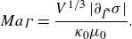 \begin{equation} {{Ma}}_\Gamma = \frac {V^{1/3}\, |\partial _{\tilde \Gamma } \sigma |}{\kappa _0 \mu _0} . \end{equation}
In order to give a physical understanding of the parameter, we consider water’s physical properties and the initial volume $V_0={5.6}\ {\unicode{x03BC} }{\textrm {l}}$
, corresponding to the initial experimental conditions of figure 1(c). Table 1 shows, in this context, the reduction of static surface tension compared to
$V_0={5.6}\ {\unicode{x03BC} }{\textrm {l}}$
, corresponding to the initial experimental conditions of figure 1(c). Table 1 shows, in this context, the reduction of static surface tension compared to $\sigma _0$
, and the corresponding
$\sigma _0$
, and the corresponding ${{Ma}}_\Gamma$
values. In the upcoming subsections, we delve into the influence of surfactants on the flow direction under specific experimental conditions. We employ the quasi-stationary model (§ 3.2) along with additional surfactants equations (5.1). To ensure accurate and physically meaningful results, we have implemented a numerical scheme that prevents negative surfactant concentrations, as detailed in Appendix A. Later on, we consolidate our findings into a comprehensive
${{Ma}}_\Gamma$
values. In the upcoming subsections, we delve into the influence of surfactants on the flow direction under specific experimental conditions. We employ the quasi-stationary model (§ 3.2) along with additional surfactants equations (5.1). To ensure accurate and physically meaningful results, we have implemented a numerical scheme that prevents negative surfactant concentrations, as detailed in Appendix A. Later on, we consolidate our findings into a comprehensive ${Ma}_T$
–
${Ma}_T$
– ${Ra}_T$
phase diagram for fixed
${Ra}_T$
phase diagram for fixed ${{Ma}}_\Gamma$
, for the flow direction assuming axial symmetry, and for the stability of the azimuthal symmetry.
${{Ma}}_\Gamma$
, for the flow direction assuming axial symmetry, and for the stability of the azimuthal symmetry.
Table 1. The ${{Ma}}_\Gamma$
values corresponding to the initial reduction of surface tension
${{Ma}}_\Gamma$
values corresponding to the initial reduction of surface tension $\Gamma _0\, |\partial _\Gamma \sigma | / \sigma _0$
at the experimental conditions.
$\Gamma _0\, |\partial _\Gamma \sigma | / \sigma _0$
at the experimental conditions.

5.1. Flow reversal at experimental conditions
Using the same experimental initial conditions as in § 4.1, we investigate the influence of surfactants on the flow direction. For a slight average reduction of 0.1 $\,\%$
of the static surface tension
$\,\%$
of the static surface tension $\sigma _0$
due to the action of surfactants, the flow follows the expected thermal Marangoni direction, from the contact line towards the apex; see figure 6(a). However, if the reduction of
$\sigma _0$
due to the action of surfactants, the flow follows the expected thermal Marangoni direction, from the contact line towards the apex; see figure 6(a). However, if the reduction of $\sigma _0$
is 0.32
$\sigma _0$
is 0.32 $\,\%$
, then a competing vortex in the opposite direction emerges; see figure 6(b). This opposing vortex is much larger if the surface tension reduction is 0.34
$\,\%$
, then a competing vortex in the opposite direction emerges; see figure 6(b). This opposing vortex is much larger if the surface tension reduction is 0.34 $\,\%$
; see figure 6(c). Finally, when the reduction reaches 0.5
$\,\%$
; see figure 6(c). Finally, when the reduction reaches 0.5 $\,\%$
, the flow completely reverses, moving from the apex towards the contact line; see figure 6(d). The findings from the study by van Gaalen et al. (Reference van Gaalen, Wijshoff, Kuerten and Diddens2022), which do not account for buoyancy-driven convection, indicate that a reduction of approximately 0.8 % in surface tension results in a substantial decrease of 99 % in interface velocity. It is noteworthy that these results are consistent with our own findings, despite the omission of buoyancy effects in their paper.
$\,\%$
, the flow completely reverses, moving from the apex towards the contact line; see figure 6(d). The findings from the study by van Gaalen et al. (Reference van Gaalen, Wijshoff, Kuerten and Diddens2022), which do not account for buoyancy-driven convection, indicate that a reduction of approximately 0.8 % in surface tension results in a substantial decrease of 99 % in interface velocity. It is noteworthy that these results are consistent with our own findings, despite the omission of buoyancy effects in their paper.

Figure 6. Influence of surfactants on the flow direction. The values (a) $0.1\,\%$
, (b)
$0.1\,\%$
, (b) $0.32\,\%$
, (c)
$0.32\,\%$
, (c) $0.34\,\%$
and (d)
$0.34\,\%$
and (d) $0.5\,\%$
are considered for the reduction of static surface tension
$0.5\,\%$
are considered for the reduction of static surface tension $| \partial _\Gamma \sigma | / \sigma _0$
. The flow direction is from the contact line towards the apex in (a). A competing vortex in the opposite direction is observed in (b) due to the increasing influence of the surfactants. There is rapid growth of the thermal Rayleigh vortex in (c). the flow is completely in the thermal Rayleigh direction in (d), with a velocity magnitude comparable to the experimental findings.
$| \partial _\Gamma \sigma | / \sigma _0$
. The flow direction is from the contact line towards the apex in (a). A competing vortex in the opposite direction is observed in (b) due to the increasing influence of the surfactants. There is rapid growth of the thermal Rayleigh vortex in (c). the flow is completely in the thermal Rayleigh direction in (d), with a velocity magnitude comparable to the experimental findings.
The velocity magnitude in figure 6(d) is comparable to both the experimental results of figure 1(b) and the hypothetical pure thermal Rayleigh flow depicted in figure 1(b). These results demonstrate that even a tiny amount of contaminants can cause a significant change in the flow direction. It is also evident that for a larger reduction of $\sigma _0$
, the distribution of the concentration of surfactants at the interface is more uniform. This is expected, as surfactants effectively reduce surface tension, resulting in weaker advective forces associated with thermal Marangoni flow. Consequently, surfactants diffuse along the interface, rather than concentrating at the apex of the droplet.
$\sigma _0$
, the distribution of the concentration of surfactants at the interface is more uniform. This is expected, as surfactants effectively reduce surface tension, resulting in weaker advective forces associated with thermal Marangoni flow. Consequently, surfactants diffuse along the interface, rather than concentrating at the apex of the droplet.
5.2. Phase diagram of the axisymmetric flow direction
When surfactants are taken into account, the phase diagram undergoes significant changes; see figure 7. Using the same colour code as in figure 4, we consider the ${{Ma}}_\Gamma$
values 0, 100, 500 and 5000. Even a slight
${{Ma}}_\Gamma$
values 0, 100, 500 and 5000. Even a slight $\sigma _0$
reduction of approximately 0.01
$\sigma _0$
reduction of approximately 0.01 $\,\%$
, corresponding to
$\,\%$
, corresponding to ${{Ma}}_\Gamma = 100$
at the conditions specified for table 1, leads to a substantial portion of the phase diagram being covered by the blue area, indicating flow in the apex towards the contact line. Remarkably, for
${{Ma}}_\Gamma = 100$
at the conditions specified for table 1, leads to a substantial portion of the phase diagram being covered by the blue area, indicating flow in the apex towards the contact line. Remarkably, for ${{Ma}}_\Gamma = 5000$
, within the considered ranges of
${{Ma}}_\Gamma = 5000$
, within the considered ranges of ${Ra}_T$
and
${Ra}_T$
and ${Ma}_T$
, the flow is almost always in the same direction as if driven by thermal buoyancy, i.e. moving from the apex towards the contact line. This corresponds to a mere
${Ma}_T$
, the flow is almost always in the same direction as if driven by thermal buoyancy, i.e. moving from the apex towards the contact line. This corresponds to a mere $\sigma _0$
reduction of approximately 0.5
$\sigma _0$
reduction of approximately 0.5 $\,\%$
. Supplementary movie 6 illustrates the change in flow direction when travelling through the different regions in the phase diagram at
$\,\%$
. Supplementary movie 6 illustrates the change in flow direction when travelling through the different regions in the phase diagram at ${{Ma}}_\Gamma =100$
.
${{Ma}}_\Gamma =100$
.
The influence of the contact angle on the direction of the flow is discussed in Appendix C.
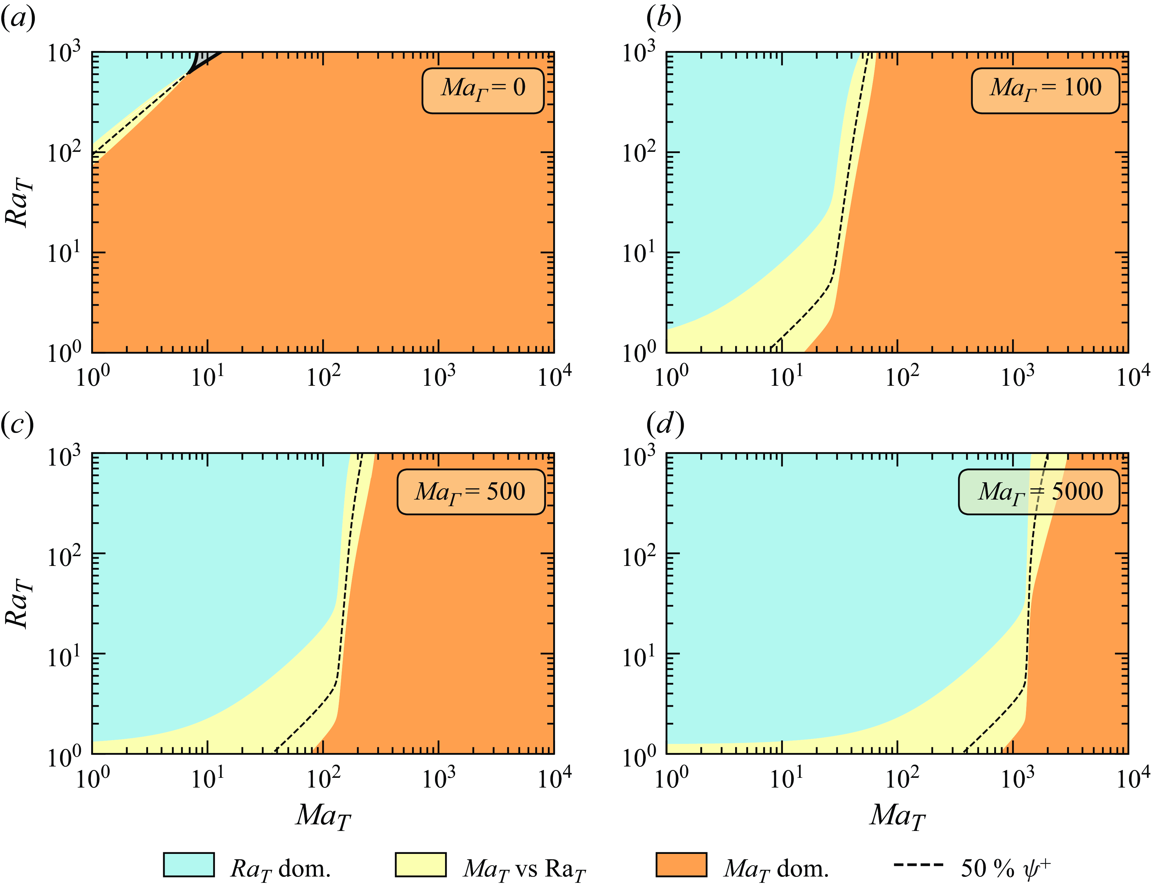
Figure 7. Flow direction phase diagram for a droplet with a contact angle $\theta = 150^\circ$
, considering the influence of surfactants at the interface, for (a)
$\theta = 150^\circ$
, considering the influence of surfactants at the interface, for (a) ${{Ma}}_\Gamma =0$
, (b)
${{Ma}}_\Gamma =0$
, (b) ${{Ma}}_\Gamma =100$
, (c)
${{Ma}}_\Gamma =100$
, (c) ${{Ma}}_\Gamma =500$
and (d)
${{Ma}}_\Gamma =500$
and (d) ${{Ma}}_\Gamma =5000$
. The blue area corresponds to
${{Ma}}_\Gamma =5000$
. The blue area corresponds to ${{Ra}}_T$
-dominated flows, the orange to
${{Ra}}_T$
-dominated flows, the orange to ${{Ma}}_T$
-dominated flows, and the yellow to a combination of both. The black dashed line corresponds to 50
${{Ma}}_T$
-dominated flows, and the yellow to a combination of both. The black dashed line corresponds to 50 $\,\%$
in volume of flow in each direction, i.e.
$\,\%$
in volume of flow in each direction, i.e. $\psi ^+=50\,\%$
.
$\psi ^+=50\,\%$
.
5.2.1. Change of slope in the $\psi ^+=50\,\%$
curve
$\psi ^+=50\,\%$
curve

Figure 7 displays a change in the slope of the $\psi ^+=50\,\%$
curve as
$\psi ^+=50\,\%$
curve as ${Ma}_T$
increases in the presence of surfactants. Notably, the quasi-stationary solutions along this curve feature two competing vortices – one driven by buoyancy, and the other by Marangoni forces – that occupy equal volumes within the droplet. We identify two distinct regimes of the curve corresponding to different slopes, for low and high
${Ma}_T$
increases in the presence of surfactants. Notably, the quasi-stationary solutions along this curve feature two competing vortices – one driven by buoyancy, and the other by Marangoni forces – that occupy equal volumes within the droplet. We identify two distinct regimes of the curve corresponding to different slopes, for low and high ${Ma}_T$
values.
${Ma}_T$
values.
To explore the impact of surfactants on this phenomenon, figure 8 examines a specific case from figure 7 with ${{Ma}}_\Gamma =100$
. The surfactants’ concentration along the droplet–gas interface is depicted for both the lower (bottom) and higher (top) regimes of the curve. Additionally, figure 8 illustrates the vortices within the droplet for each corresponding
${{Ma}}_\Gamma =100$
. The surfactants’ concentration along the droplet–gas interface is depicted for both the lower (bottom) and higher (top) regimes of the curve. Additionally, figure 8 illustrates the vortices within the droplet for each corresponding ${Ma}_T$
value and the tangential velocity
${Ma}_T$
value and the tangential velocity $u_t$
at the droplet–gas interface, plotted against the normalised arc length coordinate
$u_t$
at the droplet–gas interface, plotted against the normalised arc length coordinate $s$
, where
$s$
, where $s=0$
is at the contact line, and
$s=0$
is at the contact line, and $s=1$
is at the apex.
$s=1$
is at the apex.
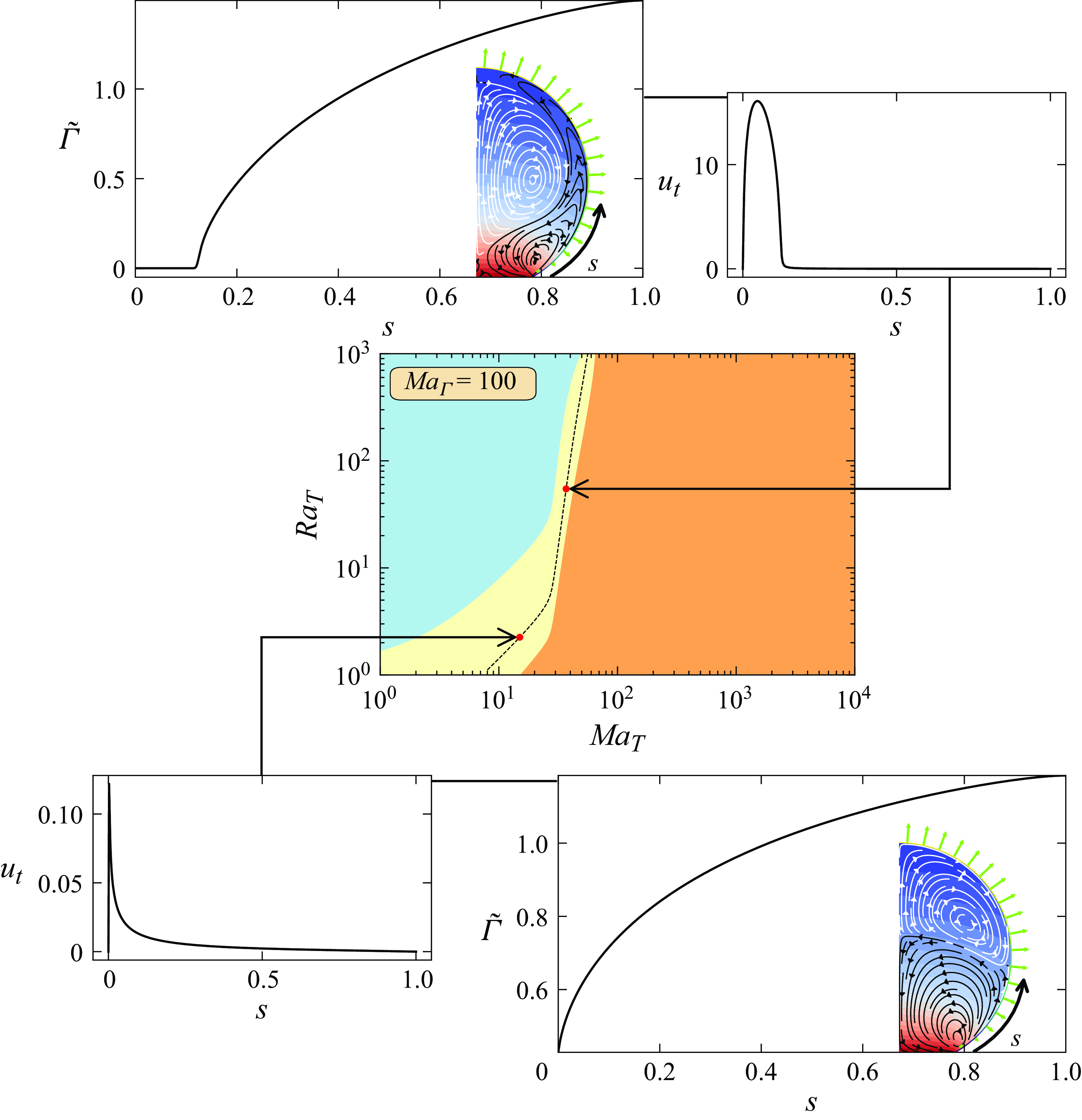
Figure 8. Surfactants’ concentration along the droplet–gas interface according to the normalised droplet–gas arc length $s$
, for
$s$
, for ${{Ma}}_\Gamma =100$
,
${{Ma}}_\Gamma =100$
, $\theta =150^\circ$
and two
$\theta =150^\circ$
and two ${Ma}_T$
, one below the threshold for which the flow reversal curve changes slope (bottom), and one above (top).
${Ma}_T$
, one below the threshold for which the flow reversal curve changes slope (bottom), and one above (top).
For low ${Ma}_T$
, the slope of the curve is approximately 1. In this regime, the vortex from the contact line towards the apex is primarily located near the droplet–gas interface, as shown at the bottom of figure 8. Thermocapillary forces counteract the effect of surfactants, resulting in a weak thermal Marangoni flow close to the interface, as depicted in the respective
${Ma}_T$
, the slope of the curve is approximately 1. In this regime, the vortex from the contact line towards the apex is primarily located near the droplet–gas interface, as shown at the bottom of figure 8. Thermocapillary forces counteract the effect of surfactants, resulting in a weak thermal Marangoni flow close to the interface, as depicted in the respective $u_t$
–
$u_t$
– $s$
plot.
$s$
plot.
As ${Ma}_T$
increases, surfactants are advected and compressed towards the droplet apex. In the high
${Ma}_T$
increases, surfactants are advected and compressed towards the droplet apex. In the high ${Ma}_T$
regime (top part of figure 8), the surfactants’ concentration at the contact line reaches zero, as shown in the respective
${Ma}_T$
regime (top part of figure 8), the surfactants’ concentration at the contact line reaches zero, as shown in the respective $\tilde {\Gamma }$
–
$\tilde {\Gamma }$
– $s$
plot for small
$s$
plot for small $s$
. Consequently, with no counteracting surfactant effect near the contact line, a strong thermal Marangoni flow emerges in that region, as indicated by the large
$s$
. Consequently, with no counteracting surfactant effect near the contact line, a strong thermal Marangoni flow emerges in that region, as indicated by the large $u_t$
in the top
$u_t$
in the top $u_t$
–
$u_t$
– $s$
plot for small
$s$
plot for small $s$
. This flow is strong enough to reverse the flow direction not only at the interface but also near the axis, as illustrated by the vortex representations.
$s$
. This flow is strong enough to reverse the flow direction not only at the interface but also near the axis, as illustrated by the vortex representations.
The change in the slope of the $\psi ^+=50\,\%$
curve is caused directly by the surfactant concentration at the contact line dropping to zero at high
$\psi ^+=50\,\%$
curve is caused directly by the surfactant concentration at the contact line dropping to zero at high ${Ma}_T$
values. In the absence of surfactants near the contact line, a strong thermal Marangoni flow develops, easily overpowering the thermal Rayleigh forces. Supplementary movie 7 provides additional visual support for this explanation.
${Ma}_T$
values. In the absence of surfactants near the contact line, a strong thermal Marangoni flow develops, easily overpowering the thermal Rayleigh forces. Supplementary movie 7 provides additional visual support for this explanation.
5.3. Axisymmetrybreaking
When surfactants are present ( ${{Ma}}_\Gamma \gt 0$
), the azimuthal symmetry of the flow is broken over a wider range of
${{Ma}}_\Gamma \gt 0$
), the azimuthal symmetry of the flow is broken over a wider range of ${Ra}_T$
and
${Ra}_T$
and ${Ma}_T$
than for the
${Ma}_T$
than for the ${{Ma}}_\Gamma =0$
case. Figure 9 presents the results of the azimuthal stability analysis for various values of
${{Ma}}_\Gamma =0$
case. Figure 9 presents the results of the azimuthal stability analysis for various values of ${{Ma}}_\Gamma$
.
${{Ma}}_\Gamma$
.
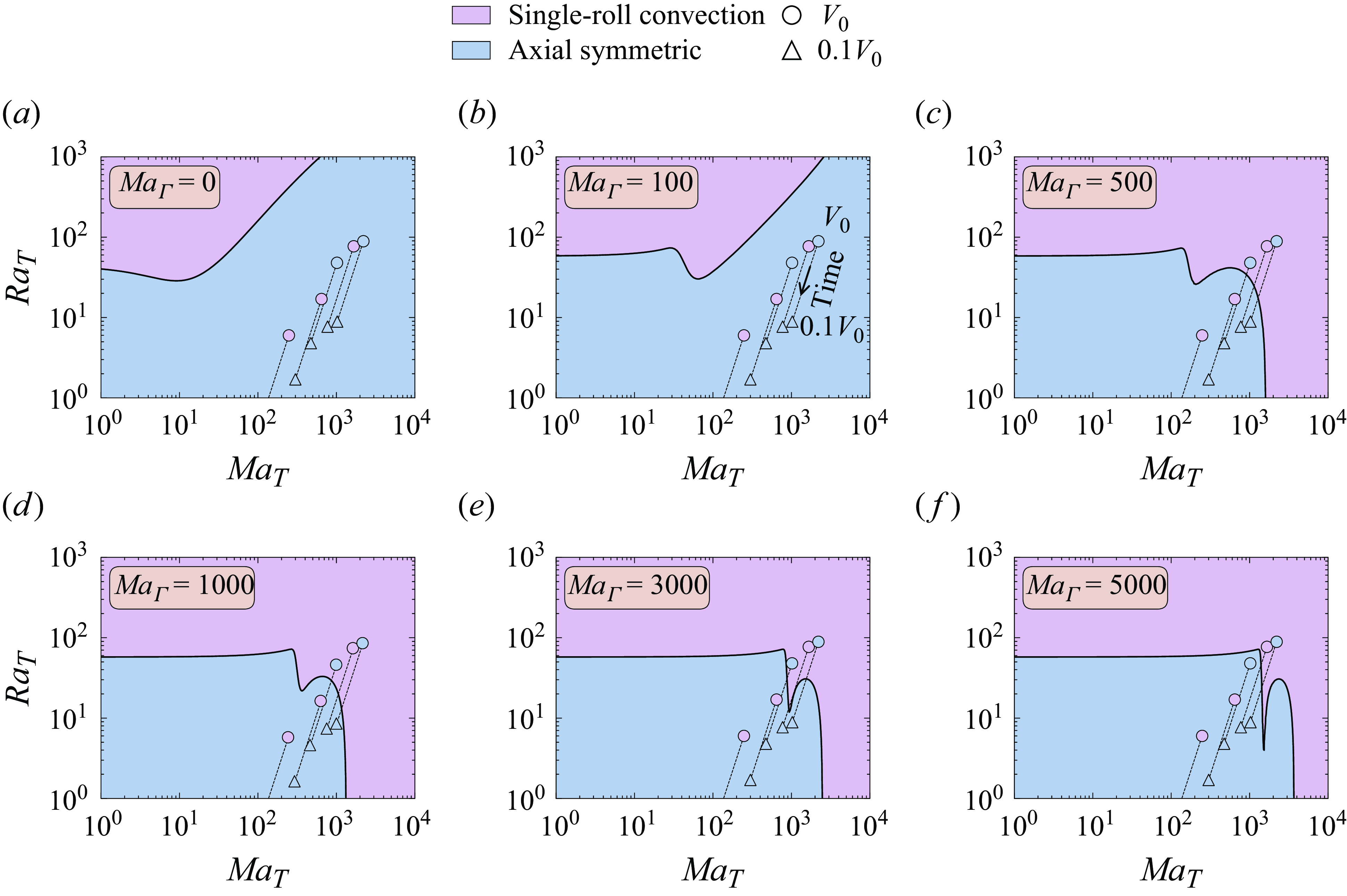
Figure 9. Stability analysis at azimuthal wavenumber $m=1$
for (a)
$m=1$
for (a) ${{Ma}}_\Gamma=0$
, (b)
${{Ma}}_\Gamma=0$
, (b) ${{Ma}}_\Gamma=100$
, (c)
${{Ma}}_\Gamma=100$
, (c) ${{Ma}}_\Gamma=500$
, (d)
${{Ma}}_\Gamma=500$
, (d) ${{Ma}}_\Gamma=1000$
, (e)
${{Ma}}_\Gamma=1000$
, (e) ${{Ma}}_\Gamma=3000$
and (f)
${{Ma}}_\Gamma=3000$
and (f) ${{Ma}}_\Gamma=5000$
of a droplet of 150
${{Ma}}_\Gamma=5000$
of a droplet of 150 $^\circ$
contact angle in a
$^\circ$
contact angle in a ${{Ra}}_T$
–
${{Ra}}_T$
– ${{Ma}}_T$
phase diagram. The black solid line represents the critical
${{Ma}}_T$
phase diagram. The black solid line represents the critical ${{Ra}}_T^c$
–
${{Ra}}_T^c$
– ${{Ma}}_T$
curve for which the flow goes from axial symmetry (blue bottom part) to single-roll convection (purple top part). The black dashed lines represent chosen experimental conditions (see supplementary movies 1–5), including those shown in figure 1.
${{Ma}}_T$
curve for which the flow goes from axial symmetry (blue bottom part) to single-roll convection (purple top part). The black dashed lines represent chosen experimental conditions (see supplementary movies 1–5), including those shown in figure 1.
Interestingly, our calculations show that for certain values of ${{Ma}}_\Gamma$
, the flow can initially exhibit asymmetric single-roll convection, and as evaporation progresses (or as the droplet volume decreases), the flow can eventually stabilise and regain axial symmetry. In figures 9(c–f), we show one single experiment that displays this behaviour while presenting quantitative agreement between experiments and numerical simulations. Nevertheless, the numerical simulations do not accurately capture the critical parameters for the transition from single-roll convection to axial symmetry across all experimental conditions. This discrepancy may be due to simplifications in the numerical model, the absence of detailed information about the surfactants’ properties, or sporadic experimental events such as contact line pinning. Although our simplified model does not allow for precise quantitative comparison with the experiments, it does provide qualitative insight into the influence of contaminants on the stability of the axisymmetric quasi-stationary solutions. For instance, when considering
${{Ma}}_\Gamma$
, the flow can initially exhibit asymmetric single-roll convection, and as evaporation progresses (or as the droplet volume decreases), the flow can eventually stabilise and regain axial symmetry. In figures 9(c–f), we show one single experiment that displays this behaviour while presenting quantitative agreement between experiments and numerical simulations. Nevertheless, the numerical simulations do not accurately capture the critical parameters for the transition from single-roll convection to axial symmetry across all experimental conditions. This discrepancy may be due to simplifications in the numerical model, the absence of detailed information about the surfactants’ properties, or sporadic experimental events such as contact line pinning. Although our simplified model does not allow for precise quantitative comparison with the experiments, it does provide qualitative insight into the influence of contaminants on the stability of the axisymmetric quasi-stationary solutions. For instance, when considering ${{Ma}}_\Gamma =100$
and sufficiently large
${{Ma}}_\Gamma =100$
and sufficiently large ${Ma}_T$
, as
${Ma}_T$
, as ${Ma}_T$
increases, the critical
${Ma}_T$
increases, the critical ${{Ra}}_T^c$
also rises, indicating that thermal Marangoni induced circulation stabilises the flow and restores axial symmetry. For
${{Ra}}_T^c$
also rises, indicating that thermal Marangoni induced circulation stabilises the flow and restores axial symmetry. For ${Ma}_\Gamma \gtrapprox 500$
, the bifurcation curve becomes independent of
${Ma}_\Gamma \gtrapprox 500$
, the bifurcation curve becomes independent of ${Ma}_T$
in the limit of low
${Ma}_T$
in the limit of low ${Ma}_T$
. However, for larger
${Ma}_T$
. However, for larger ${Ma}_T$
, the critical
${Ma}_T$
, the critical ${Ra}_T^c$
decreases with increasing
${Ra}_T^c$
decreases with increasing ${Ma}_T$
, suggesting that the combined effects of solutal and thermal Marangoni forces destabilise the flow and break axial symmetry.
${Ma}_T$
, suggesting that the combined effects of solutal and thermal Marangoni forces destabilise the flow and break axial symmetry.
In the next subsection, we further explore the influence of the contact angle on the azimuthal symmetry-breaking phenomenon. To simplify the problem, we isolate the thermal Rayleigh effects ( ${Ma}_T={Ma}_\Gamma =0$
) and focus on examining how the large contact angle affects azimuthal symmetry breaking.
${Ma}_T={Ma}_\Gamma =0$
) and focus on examining how the large contact angle affects azimuthal symmetry breaking.
5.4. Contact angle influence in axisymmetrybreaking: pure Rayleigh flow
We present ${Ra}_T^c$
for a range of
${Ra}_T^c$
for a range of $\theta$
, from
$\theta$
, from $85^\circ$
to
$85^\circ$
to $179^\circ$
, in figure 10, considering
$179^\circ$
, in figure 10, considering ${Ma}_T={Ma}_\Gamma =0$
. At the left of the figure, the convective roll flow field at
${Ma}_T={Ma}_\Gamma =0$
. At the left of the figure, the convective roll flow field at $\theta =87^\circ$
is shown, and at the right, the flow field at
$\theta =87^\circ$
is shown, and at the right, the flow field at $\theta =179^\circ$
. Obviously – and as the flow field representations reflects – for droplets of fixed volume, the contact radius will be much larger if the contact angle is smaller. The contact area with the substrate, which has fixed temperature and is perfectly conducting, is much smaller for larger
$\theta =179^\circ$
. Obviously – and as the flow field representations reflects – for droplets of fixed volume, the contact radius will be much larger if the contact angle is smaller. The contact area with the substrate, which has fixed temperature and is perfectly conducting, is much smaller for larger $\theta$
, which will result in a larger temperature gradient within the droplet. As
$\theta$
, which will result in a larger temperature gradient within the droplet. As $\theta \rightarrow 180^\circ$
, the contact radius reduces to zero, approaching a heat point source. At the same time, an increasing contact angle reduces the size of the no-slip boundary condition at the substrate, thereby allowing for single-roll convection, which is almost free from viscous forces in the limit
$\theta \rightarrow 180^\circ$
, the contact radius reduces to zero, approaching a heat point source. At the same time, an increasing contact angle reduces the size of the no-slip boundary condition at the substrate, thereby allowing for single-roll convection, which is almost free from viscous forces in the limit $\theta \rightarrow 180^\circ$
.
$\theta \rightarrow 180^\circ$
.

Figure 10. Critical ${Ra}_T^c$
for different contact angles
${Ra}_T^c$
for different contact angles $\theta$
for the
$\theta$
for the $m=1$
instability to happen, for
$m=1$
instability to happen, for ${Ma}_\Gamma ={Ma}_T=0$
. The black solid line represents the
${Ma}_\Gamma ={Ma}_T=0$
. The black solid line represents the ${Ra}_T^c$
–
${Ra}_T^c$
– ${Ma}_T$
curve for which the flow goes from axial symmetry (blue bottom part) to single-roll convection (purple top part).
${Ma}_T$
curve for which the flow goes from axial symmetry (blue bottom part) to single-roll convection (purple top part).
As the contact angle increases, ${Ra}_T^c$
decreases, indicating that the large contact angle contributes to the azimuthal instability of the flow, similar to the onset of Rayleigh–Bénard convection in a cylindrical container with aspect ratio 1. To further support this hypothesis, we considered a theoretical scenario with no thermal buoyancy effects (
${Ra}_T^c$
decreases, indicating that the large contact angle contributes to the azimuthal instability of the flow, similar to the onset of Rayleigh–Bénard convection in a cylindrical container with aspect ratio 1. To further support this hypothesis, we considered a theoretical scenario with no thermal buoyancy effects ( ${Ra}_T={Ma}_\Gamma =0$
), only thermal Marangoni effects. The resulting solution of the azimuthal eigenvalue problem shows that flow is always stable in the azimuthal direction, independently of
${Ra}_T={Ma}_\Gamma =0$
), only thermal Marangoni effects. The resulting solution of the azimuthal eigenvalue problem shows that flow is always stable in the azimuthal direction, independently of ${Ma}_T$
. Surfactants thus play a key role in the complex large
${Ma}_T$
. Surfactants thus play a key role in the complex large ${Ma}_T$
azimuthal symmetry-breaking phenomenon depicted in figures 9(c–f), as concluded from the results of this section.
${Ma}_T$
azimuthal symmetry-breaking phenomenon depicted in figures 9(c–f), as concluded from the results of this section.
For shallow droplets (small contact angle), thermal Marangoni instabilities are expected to induce highly non-axisymmetric flow patterns (Babor & Kuhlmann Reference Babor and Kuhlmann2023), also known as hydrothermal waves (Sefiane et al. Reference Sefiane, Moffat, Matar and Craster2008), which usually appear on heated substrates. Solutal Marangoni flow can exhibit even more asymmetric and even chaotic flow, as e.g. observed in evaporating ethanol–water droplets (Diddens et al. Reference Diddens, Tan, Lv, Versluis, Kuerten, Zhang and Lohse2017b ). Since these phenomena are not observed in water droplets at ambient conditions, they are beyond the scope of this paper.
6. Outlook
Evaporating pure water droplets sitting on thermally conductive substrates exhibit, due to evaporative cooling, a temperature gradient within the droplet and along its droplet–gas interface. As a result, an interplay between buoyant and thermocapillary forces is expected. Previous theoretical and numerical predictions (Hu & Larson Reference Hu and Larson2005; Sáenz et al. Reference Sáenz, Sefiane, Kim, Matar and Valluri2015; Diddens et al. Reference Diddens, Tan, Lv, Versluis, Kuerten, Zhang and Lohse2017b ), as well as our simulations, show that thermocapillary forces are dominant for small droplets, resulting in an interfacial thermally driven Marangoni flow directed from the contact line towards the apex. However, previous experimental observations (Buffone & Sefiane Reference Buffone and Sefiane2004; Marin et al. Reference Marin, Liepelt, Rossi and Kähler2016; Diddens et al. Reference Diddens, Tan, Lv, Versluis, Kuerten, Zhang and Lohse2017b ; Rossi et al. Reference Rossi, Marin and Kähler2019), and our own measurements shown in § 2, reveal that the thermally driven Marangoni flow is hindered by the presence of surfactants (when added intentionally) or contaminants (when their presence is unintentional). In the case at hand, we show that thermally driven Marangoni flows are rarely seen, and when present, their strength is orders of magnitude lower than expected.
A detailed transient model for a clean, pure water droplet was initially used to perform numerical simulations under the same conditions as in the experiments. The numerical results showed a significant discrepancy when compared to the experimental data. To address this, a small amount of insoluble surfactants was introduced in the axisymmetric numerical simulations. This adjustment led to a shift in the flow direction, aligning it with the thermal Rayleigh flow observed in most experiments, even when using a simplified quasi-stationary model. Additionally, the quasi-stationary approach was employed to generate ${Ma}_T$
–
${Ma}_T$
– ${Ra}_T$
phase diagrams for the flow direction under the assumption of axisymmetry, and to analyse the azimuthal stability at an azimuthal wavenumber
${Ra}_T$
phase diagrams for the flow direction under the assumption of axisymmetry, and to analyse the azimuthal stability at an azimuthal wavenumber $m = 1$
, for both pure and contaminated water cases.
$m = 1$
, for both pure and contaminated water cases.
At specified initial experimental conditions, as those shown in figure 1(c), a mere 0.5 $\,\%$
reduction in the static surface tension was sufficient to reverse the flow direction, agreeing remarkably well with the results of van Gaalen et al. (Reference van Gaalen, Wijshoff, Kuerten and Diddens2022), despite their work not considering buoyancy-driven convection. When surfactants are considered, the phase diagram for the flow direction undergoes significant changes, even for small
$\,\%$
reduction in the static surface tension was sufficient to reverse the flow direction, agreeing remarkably well with the results of van Gaalen et al. (Reference van Gaalen, Wijshoff, Kuerten and Diddens2022), despite their work not considering buoyancy-driven convection. When surfactants are considered, the phase diagram for the flow direction undergoes significant changes, even for small ${Ma}_\Gamma$
. This indicates that a larger set of parameters within the considered phase space will show a vortex from the apex towards the contact line. Within this phase space, as
${Ma}_\Gamma$
. This indicates that a larger set of parameters within the considered phase space will show a vortex from the apex towards the contact line. Within this phase space, as ${Ma}_T$
rises, the accumulation of surfactants at the apex increases up to a point where no surfactants are present close to the contact line. A strong thermal Marangoni flow emerges in this region, rapidly reversing the flow upon a slight increase in
${Ma}_T$
rises, the accumulation of surfactants at the apex increases up to a point where no surfactants are present close to the contact line. A strong thermal Marangoni flow emerges in this region, rapidly reversing the flow upon a slight increase in ${Ma}_T$
. For smaller
${Ma}_T$
. For smaller $\theta$
, the thermal profile within the droplet is more uniform due to the larger contact radius and smaller apex height. When surfactants are considered, a larger
$\theta$
, the thermal profile within the droplet is more uniform due to the larger contact radius and smaller apex height. When surfactants are considered, a larger ${Ma}_T$
is required for the droplet to present a vortex from the contact line towards the apex, as long as
${Ma}_T$
is required for the droplet to present a vortex from the contact line towards the apex, as long as ${Ra}_T$
is sufficiently big. The onset of
${Ra}_T$
is sufficiently big. The onset of $m=1$
asymmetry is significantly affected by the presence of surfactants. For certain
$m=1$
asymmetry is significantly affected by the presence of surfactants. For certain ${Ma}_\Gamma$
values, the flow can initially show asymmetric single-roll convection, but as evaporation progresses, it may stabilise and regain axial symmetry. This numerically found behaviour matches that of the majority of our experiments, though the numerical simulations do not precisely capture the critical parameters for the transition to axial symmetry in all experiments. Despite the model’s simplicity , it provides a unique insight into the influence of contaminants on the stability of axisymmetric solutions. For
${Ma}_\Gamma$
values, the flow can initially show asymmetric single-roll convection, but as evaporation progresses, it may stabilise and regain axial symmetry. This numerically found behaviour matches that of the majority of our experiments, though the numerical simulations do not precisely capture the critical parameters for the transition to axial symmetry in all experiments. Despite the model’s simplicity , it provides a unique insight into the influence of contaminants on the stability of axisymmetric solutions. For ${Ma}_\Gamma =100$
and large
${Ma}_\Gamma =100$
and large ${Ma}_T$
, the critical
${Ma}_T$
, the critical ${Ra}_T^c$
increases, suggesting that thermal Marangoni circulation stabilises the flow and restores symmetry. For
${Ra}_T^c$
increases, suggesting that thermal Marangoni circulation stabilises the flow and restores symmetry. For ${Ma}_\Gamma \gtrapprox 500$
, the bifurcation curve becomes independent of
${Ma}_\Gamma \gtrapprox 500$
, the bifurcation curve becomes independent of ${Ma}_T$
at lower values. This implies that in a droplet with contact angle
${Ma}_T$
at lower values. This implies that in a droplet with contact angle $150^\circ$
, the flow asymmetry is closely linked to
$150^\circ$
, the flow asymmetry is closely linked to ${Ra}_T$
. In ideal scenarios in the absence of contamination or surfactants, our analysis predicts a single convective roll at lower
${Ra}_T$
. In ideal scenarios in the absence of contamination or surfactants, our analysis predicts a single convective roll at lower $Ra_T^c$
for larger contact angles, indicating that the large contact angle contributes to azimuthal instability. However, for larger
$Ra_T^c$
for larger contact angles, indicating that the large contact angle contributes to azimuthal instability. However, for larger ${Ma}_T$
and
${Ma}_T$
and ${Ma}_\Gamma \gtrapprox 500$
, the critical
${Ma}_\Gamma \gtrapprox 500$
, the critical ${Ra}_T^c$
decreases, showing that combined solutal and thermal Marangoni forces destabilise the flow and break symmetry.
${Ra}_T^c$
decreases, showing that combined solutal and thermal Marangoni forces destabilise the flow and break symmetry.
Contaminants thus induce a significant change in the flow features. The source of the contamination acting as surfactants is yet unknown, but can likely be found in both the original particle solutions (unavoidable to certain degree in the production process) and the environment (organic material in the room’s air).
The propensity of water–air interfaces to become polluted has been reported in multiple systems in the past, from rising bubbles (Manikantan & Squires Reference Manikantan and Squires2020) to liquid bridges (Ponce-Torres et al. Reference Ponce-Torres, Vega and Montañero2016), and its prevention has always encountered only minor success. The impact of contamination from the particle solution can be mitigated by carefully washing the particle solution in multiple iterations. The results, however, show a even larger variety of flow patterns (including fading thermocapillary flows) than those observed with unwashed solutions, revealing a higher sensitivity of the interface to contamination from the environment, and in agreement with the results of Kazemi et al. (Reference Kazemi, Saber, Elliott and Nobes2021). The thermocapillary flows observed under those conditions always quickly evolved into convective buoyant flow patterns during the evaporation process, denoting a likely increase in contamination over time in those conditions. Looking at the experimental results, the degree of contamination seemed more consistent for unwashed solutions. Therefore, we decided to show only those experimental results in this work. The issue with different degrees of contamination will be a topic for a future work.
Although the present work, as well as Hu & Larson (Reference Hu and Larson2005) and van Gaalen et al. (Reference van Gaalen, Wijshoff, Kuerten and Diddens2022), provides a reasonable explanation for the absence of thermal Marangoni flow in evaporating water droplets, the presence of surfactants in multi-component droplets is still unexplored. The presence of contaminants in glycerol–water mixtures has been attributed as the cause for the formation of Marangoni rings upon evaporation (Thayyil Raju et al. Reference Thayyil Raju, Diddens, Li, Marin, van der Linden, Zhang and Lohse2022), but to the best of our knowledge, the influence of surfactants on the flow patterns in such mixtures has not yet been investigated quantitatively.
Supplementary movies
Supplementary movies are available at https://doi.org/10.1017/jfm.2025.10208.
Acknowledgements
The authors would like to give a special acknowledgment to C. Seyfert, whose sharp eye detected this phenomenon for the first time, and her careful experiments inspired this paper. We are thankful to Y. Jiang (exchange fellow USTC) and S. Galas (exchange ENS Paris Saclay), who obtained the shown particular experimental data set during their internships in our labs.
Funding
This work was supported by an Industrial Partnership Programme of the Netherlands Organisation for Scientific Research (NWO) & High Tech Systems and Materials (HTSM), co-financed by Canon Production Printing Netherlands B.V., University of Twente, and Eindhoven University of Technology (project TKI HTSM – CANON – P1 – PRINTHEAD & DROPLET FORMATION, grant no. PPS2107). A.M. acknowledges funding by the European Research Council under the Horizon Europe programme (project NanoPlastBall, grant no. 101101022).
Declaration of interests
The authors report no conflict of interest.
Appendix A. Spatial discretisation
Both the droplet domain $\Omega$
and the gas domain
$\Omega$
and the gas domain $\Omega ^{{gas}}$
are partitioned into a triangular mesh composed of elements
$\Omega ^{{gas}}$
are partitioned into a triangular mesh composed of elements $\mathcal{T}_h$
and
$\mathcal{T}_h$
and $\mathcal{T}^{{gas}}_h$
. The
$\mathcal{T}^{{gas}}_h$
. The $\Gamma$
-field is present only at the two-dimensional droplet–gas interface,
$\Gamma$
-field is present only at the two-dimensional droplet–gas interface, $\tau = \partial \Omega$
. When considering an axial symmetric coordinate system,
$\tau = \partial \Omega$
. When considering an axial symmetric coordinate system, $\Gamma$
is present only on a one-dimensional curved line, therefore embedded in a two-dimensional space. We denote the set of one-dimensional elements composing the interface as
$\Gamma$
is present only on a one-dimensional curved line, therefore embedded in a two-dimensional space. We denote the set of one-dimensional elements composing the interface as $\mathcal{I}_h$
, and denote by
$\mathcal{I}_h$
, and denote by $\mathcal{F}_h$
the set of nodes (vertices) on
$\mathcal{F}_h$
the set of nodes (vertices) on $\tau$
, which is also referred to as the skeleton of the (one-dimensional) triangulation
$\tau$
, which is also referred to as the skeleton of the (one-dimensional) triangulation $\mathcal{I}_h$
.
$\mathcal{I}_h$
.
A.1. Approximation of surfactants’ concentration
The transport equation of the surfactants’ concentration $\Gamma$
, (5.1), can be associated with a high Péclet number, which makes it difficult to solve numerically (Donea & Huerta Reference Donea and Huerta2003). So we chose a locally bound preserving discretisation that can be interpreted as a face-centred finite volume method; see Eymard, Gallouët & Herbin (Reference Eymard, Gallouët and Herbin2000) and Vieira et al. (Reference Vieira, Giacomini, Sevilla and Huerta2020). The surfactants’ concentration is approximated at the midpoint (centre) of elements in
$\Gamma$
, (5.1), can be associated with a high Péclet number, which makes it difficult to solve numerically (Donea & Huerta Reference Donea and Huerta2003). So we chose a locally bound preserving discretisation that can be interpreted as a face-centred finite volume method; see Eymard, Gallouët & Herbin (Reference Eymard, Gallouët and Herbin2000) and Vieira et al. (Reference Vieira, Giacomini, Sevilla and Huerta2020). The surfactants’ concentration is approximated at the midpoint (centre) of elements in $\mathcal{I}_h$
, and additionally at vertices
$\mathcal{I}_h$
, and additionally at vertices $V \in \mathcal{F}_h$
. We define the spaces
$V \in \mathcal{F}_h$
. We define the spaces
 \begin{align} G_h = \{ \gamma _h \in \mathbb{P}^0(I), \textrm { for all } I \in \mathcal{I}_h \} \quad \textrm {and} \quad \hat G_h = \{ \hat \gamma _h \in \mathbb{P}^0(V), \textrm { for all } V \in \mathcal{F}_h \}, \end{align}
where $\mathbb{P}^l(\omega ),\ l\geqslant 0$
, corresponds to the space of polynomials of degree
$\mathbb{P}^l(\omega ),\ l\geqslant 0$
, corresponds to the space of polynomials of degree $l$
defined on a given domain
$l$
defined on a given domain $\omega$
.
$\omega$
.
Considering $\gamma _h$
and
$\gamma _h$
and $\hat {\gamma }_h$
as the discrete test functions of the spaces
$\hat {\gamma }_h$
as the discrete test functions of the spaces $G_h$
and
$G_h$
and $\hat {G}_h$
, we define the following weak formulation for the surfactants’ concentration transport equation (5.1):
$\hat {G}_h$
, we define the following weak formulation for the surfactants’ concentration transport equation (5.1):
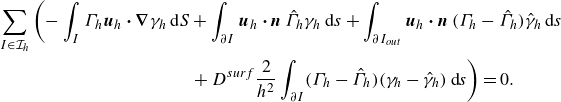 \begin{align} &\sum _{I \in \mathcal{I}_h} \left ( -\int _{I} \Gamma _h \boldsymbol{u}_h \boldsymbol \cdot \boldsymbol \nabla \gamma _h\, {\textrm d}S + \int _{{\partial I}} \boldsymbol{u}_h \boldsymbol \cdot \boldsymbol{n}\, \hat {\Gamma} _h\gamma _h\, {\textrm d}s + \int _{\partial I_{{out}}} \boldsymbol{u}_h \boldsymbol \cdot \boldsymbol{n}\, (\Gamma _h - \hat {\Gamma} _h) {\hat \gamma }_h\, {\textrm d}s \right . \nonumber \\&\!\!\qquad\qquad\qquad\qquad\qquad\quad\left . {}+ D^{{surf}} \dfrac {2}{h^2} \int _{\partial I} (\Gamma _h - \hat {\Gamma }_h)(\gamma _h - \hat {\gamma }_h)\, {\textrm d}s \right )= 0 . \end{align}
Here, the first three terms correspond to the convection, while the last term describes the diffusion. Note that due to the element-wise constant approximation, the first integral vanishes. The vector $\boldsymbol{n}$
denotes the outward-pointing normal vector of an element
$\boldsymbol{n}$
denotes the outward-pointing normal vector of an element $I$
(defined at the vertices of
$I$
(defined at the vertices of $I$
, i.e. tangential to the interface), and
$I$
, i.e. tangential to the interface), and $\partial I$
reads as the two endpoints (vertices) of
$\partial I$
reads as the two endpoints (vertices) of $I$
. An outflow boundary
$I$
. An outflow boundary $\partial I_{{out}}$
is understood as an endpoint where
$\partial I_{{out}}$
is understood as an endpoint where $\boldsymbol{u}_h \boldsymbol \cdot \boldsymbol{n} \geqslant 0$
. Further note that an integral of the form
$\boldsymbol{u}_h \boldsymbol \cdot \boldsymbol{n} \geqslant 0$
. Further note that an integral of the form $\int _{\partial I} \cdot\ {\textrm d}s$
actually reads as point evaluations at the two endpoints. Testing the equation solely with test functions
$\int _{\partial I} \cdot\ {\textrm d}s$
actually reads as point evaluations at the two endpoints. Testing the equation solely with test functions ${\hat \gamma }_h$
, it is easy to see that (for
${\hat \gamma }_h$
, it is easy to see that (for $D^{{surf}} = 0$
) the trace approximation
$D^{{surf}} = 0$
) the trace approximation ${\hat \Gamma }_h$
corresponds to the upwind value, thus we consider an upwind stabilised convection formulation. As is known from finite volume methods (and lowest-order discontinuous Galerkin methods; see Eymard et al. Reference Eymard, Gallouët and Herbin2000; Kuzmin & Hajduk Reference Kuzmin and Hajduk2023), this results in a locally conservative method, and the approximated values of
${\hat \Gamma }_h$
corresponds to the upwind value, thus we consider an upwind stabilised convection formulation. As is known from finite volume methods (and lowest-order discontinuous Galerkin methods; see Eymard et al. Reference Eymard, Gallouët and Herbin2000; Kuzmin & Hajduk Reference Kuzmin and Hajduk2023), this results in a locally conservative method, and the approximated values of $\Gamma _h$
will stay positive. We further want to emphasise the factor
$\Gamma _h$
will stay positive. We further want to emphasise the factor $2$
in the diffusive bilinear form, which results from considering finite differences between the element midpoint (approximated via
$2$
in the diffusive bilinear form, which results from considering finite differences between the element midpoint (approximated via $\Gamma _h$
) and the trace at the boundary
$\Gamma _h$
) and the trace at the boundary ${\hat \Gamma }_h$
(which are apart by
${\hat \Gamma }_h$
(which are apart by $h/2$
, where
$h/2$
, where $h$
is the length of the element
$h$
is the length of the element $I$
).
$I$
).
A.2. Approximation of the flow velocity, pressure, temperature and vapour concentration
The approximation of the Stokes problem is based on the MINI finite element method (see Boffi, Brezzi & Fortin Reference Boffi, Brezzi and Fortin2013), i.e. we approximate the velocity and the pressure in the spaces
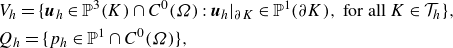 \begin{align} & V_h = \{\boldsymbol{u}_h \in \mathbb{P}^3(K)\cap C^0(\Omega ): \boldsymbol{u}_h|_{\partial K} \in \mathbb{P}^1(\partial K), \textrm { for all } K \in \mathcal{T}_h\}, \nonumber \\ & Q_h = \{ p_h \in \mathbb{P}^1 \cap C^0(\Omega )\}, \end{align}
respectively. Thus the velocity is element-wise approximated by linear functions, including the local element bubble (a cubic polynomial that vanishes at element boundaries $\partial K$
). We have chosen this discretisation because numerical experiments showed that it is essential that the (surface) gradient of the velocity (for the MINI-element resulting in an element-wise constant since the bubble part vanishes) matches the approximation space
$\partial K$
). We have chosen this discretisation because numerical experiments showed that it is essential that the (surface) gradient of the velocity (for the MINI-element resulting in an element-wise constant since the bubble part vanishes) matches the approximation space $G_h$
. Although other combinations are numerically stable, they resulted in oscillations in the tangential velocity.
$G_h$
. Although other combinations are numerically stable, they resulted in oscillations in the tangential velocity.
As already noted in § 3.3, both the temperature and vapour concentration are discretised by a standard first-order Lagrangian finite element method.
Appendix B. Dependence on Lewis number
In the results of figure 7, we have considered a fixed surface diffusivity 10 $^{-9}$
m
$^{-9}$
m $^2$
s–1, i.e.
$^2$
s–1, i.e. ${Le}\sim10^2$
. Although this assumption is made, the unknown source of the surfactants makes it difficult to determine a valid
${Le}\sim10^2$
. Although this assumption is made, the unknown source of the surfactants makes it difficult to determine a valid ${Le}$
value. Notably, its influence on the flow direction is not expected to be entirely negligible. Figure 11 shows the
${Le}$
value. Notably, its influence on the flow direction is not expected to be entirely negligible. Figure 11 shows the ${Ma}_T$
–
${Ma}_T$
– ${Ra}_T$
phase diagram for flow direction for a droplet of 150
${Ra}_T$
phase diagram for flow direction for a droplet of 150 $^\circ$
contact angle and
$^\circ$
contact angle and ${Ma}_\Gamma=500$
, considering
${Ma}_\Gamma=500$
, considering ${Le}=10^1$
(red),
${Le}=10^1$
(red), ${Le}=10^2$
(black, value taken in results of figure 7),
${Le}=10^2$
(black, value taken in results of figure 7), ${Le}=10^3$
(blue) and
${Le}=10^3$
(blue) and ${Le}=10^4$
(green).
${Le}=10^4$
(green).
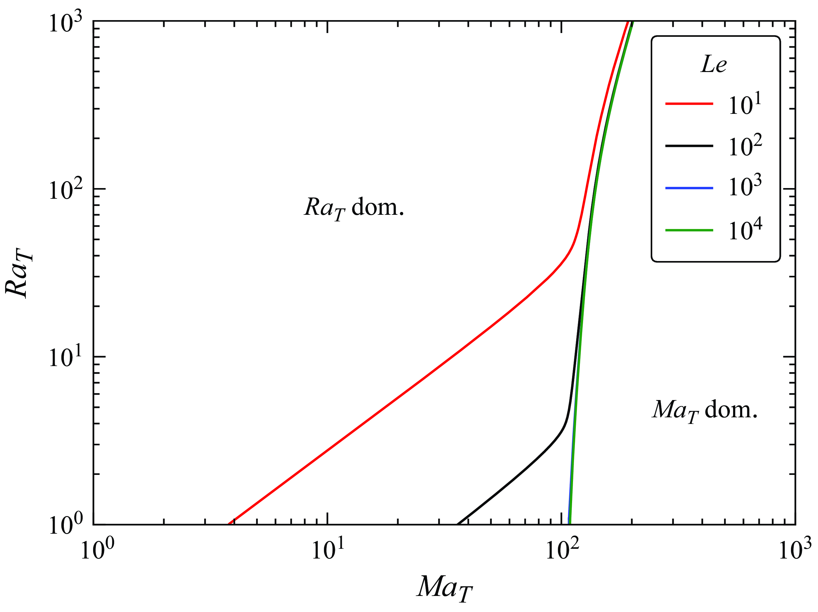
Figure 11. The ${Ma}_T$
–
${Ma}_T$
– ${Ra}_T$
phase diagram for flow direction for a droplet of 150
${Ra}_T$
phase diagram for flow direction for a droplet of 150 $^\circ$
contact angle and
$^\circ$
contact angle and ${Ma}_\Gamma=500$
, considering
${Ma}_\Gamma=500$
, considering ${Le}=10^1$
(red),
${Le}=10^1$
(red), ${Le}=10^2$
(black, value taken in results of figure 7),
${Le}=10^2$
(black, value taken in results of figure 7), ${Le}=10^3$
(blue) and
${Le}=10^3$
(blue) and ${Le}=10^4$
(green).
${Le}=10^4$
(green).
On the one hand, higher diffusivity in the transport equation (5.1), i.e. lower ${Le}$
, implies a weaker transport of surfactants by interfacial velocity towards the apex. At the apex, for high contact angles, thermal gradients are more intense. If the accumulation of the surfactants at the apex is weaker, then the surface tension gradient due to thermal effects will be stronger, therefore leading to a more pronounced thermal Marangoni flow. On the other hand, a lower diffusivity weakens the thermal Marangoni flow. However, a large compression of the surfactants leads to reaching a zero concentration at the contact line for lower
${Le}$
, implies a weaker transport of surfactants by interfacial velocity towards the apex. At the apex, for high contact angles, thermal gradients are more intense. If the accumulation of the surfactants at the apex is weaker, then the surface tension gradient due to thermal effects will be stronger, therefore leading to a more pronounced thermal Marangoni flow. On the other hand, a lower diffusivity weakens the thermal Marangoni flow. However, a large compression of the surfactants leads to reaching a zero concentration at the contact line for lower ${Ma}_T$
. Thereby, the flow reversal curve happens when
${Ma}_T$
. Thereby, the flow reversal curve happens when ${Ma}_T$
is strong enough to push the surfactants away from the contact line, allowing it to grow and develop a strong flow close to the contact line.
${Ma}_T$
is strong enough to push the surfactants away from the contact line, allowing it to grow and develop a strong flow close to the contact line.
Appendix C. Contact angle influence on axisymmetric flow direction
The spatial scaling for the dimensionless equations is based on the volume of the droplet. The contact angle is then another parameter that can influence the flow direction. We investigate here the impact of $\theta$
on the flow direction in the
$\theta$
on the flow direction in the ${Ra}_T$
–
${Ra}_T$
– ${Ma}_T$
phase diagram for droplets of the same volume. For
${Ma}_T$
phase diagram for droplets of the same volume. For $\theta\lt 90^\circ$
, even though the evaporation rate is higher at the contact line, the temperature at the apex is still lower if we assume the substrate to be perfectly conductive during the evaporation process. In such cases, the thermal Marangoni flow will have the same direction as for higher
$\theta\lt 90^\circ$
, even though the evaporation rate is higher at the contact line, the temperature at the apex is still lower if we assume the substrate to be perfectly conductive during the evaporation process. In such cases, the thermal Marangoni flow will have the same direction as for higher $\theta$
, i.e. from the contact line towards the apex.
$\theta$
, i.e. from the contact line towards the apex.
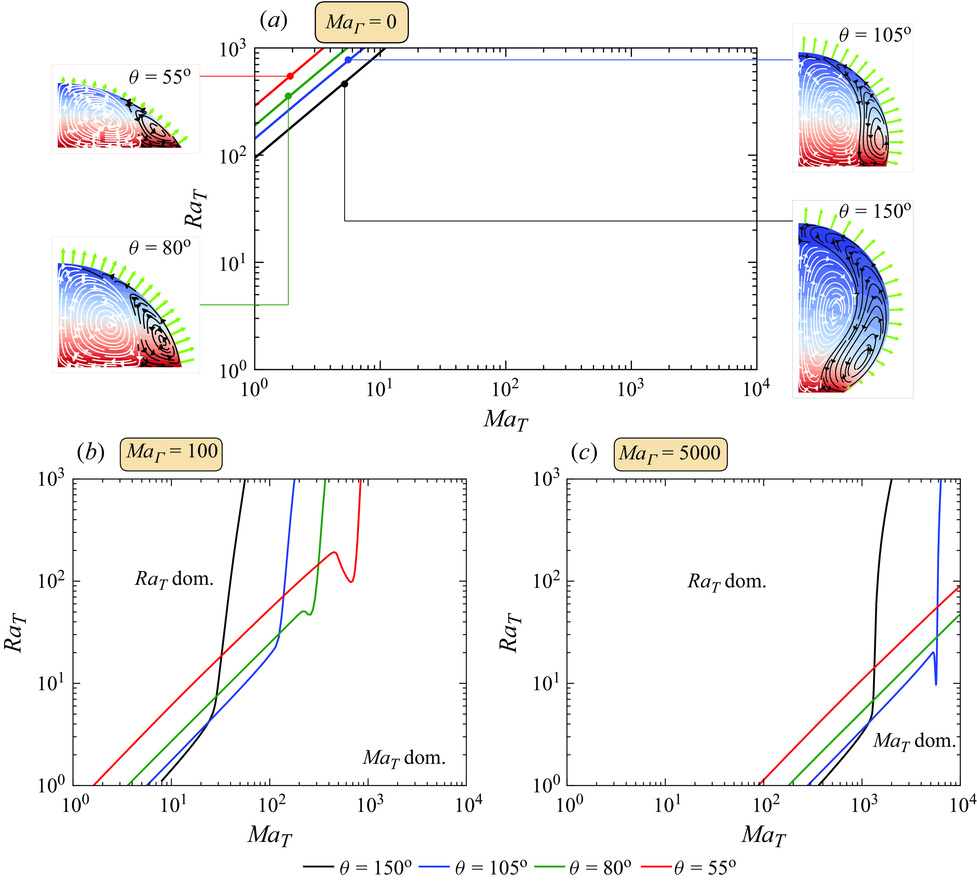
Figure 12. Flow reversal curves (i.e. $\psi =50\,\%$
) in the
$\psi =50\,\%$
) in the ${Ma}_T$
–
${Ma}_T$
– ${Ra}_T$
phase diagram for
${Ra}_T$
phase diagram for $\theta$
values 150
$\theta$
values 150 $^\circ$
(black), 105
$^\circ$
(black), 105 $^\circ$
(blue), 80
$^\circ$
(blue), 80 $^\circ$
(green) and 55
$^\circ$
(green) and 55 $^\circ$
(red), and
$^\circ$
(red), and ${Ma}_\Gamma$
values (a) 0, (b) 100 and (c) 5000. In (a), the insets show the flow scenario in the droplet for parameters directly on the reversal curve, for each respective contact angle.
${Ma}_\Gamma$
values (a) 0, (b) 100 and (c) 5000. In (a), the insets show the flow scenario in the droplet for parameters directly on the reversal curve, for each respective contact angle.
Figure 12 illustrates the $\psi ^+=50\,\%$
curves. The curves are shown for contact angles
$\psi ^+=50\,\%$
curves. The curves are shown for contact angles $55^\circ$
(red),
$55^\circ$
(red), $80^\circ$
(green),
$80^\circ$
(green), $105^\circ$
(blue), and the reference
$105^\circ$
(blue), and the reference $150^\circ$
(black), for
$150^\circ$
(black), for ${Ma}_\Gamma$
values 0, 100 and 5000. When
${Ma}_\Gamma$
values 0, 100 and 5000. When ${Ma}_\Gamma = 0$
, for the flow to be from the contact line towards the apex, lower
${Ma}_\Gamma = 0$
, for the flow to be from the contact line towards the apex, lower $\theta$
requires
$\theta$
requires ${Ra}_T$
to be larger, for a fixed
${Ra}_T$
to be larger, for a fixed ${Ma}_T$
. This is expected since the temperature gradient is directly related to the height and contact radius of the droplet, which are respectively smaller and larger for droplets of the same volume with lower
${Ma}_T$
. This is expected since the temperature gradient is directly related to the height and contact radius of the droplet, which are respectively smaller and larger for droplets of the same volume with lower $\theta$
. Lower thermal Rayleigh effects are therefore expected for the latter case.
$\theta$
. Lower thermal Rayleigh effects are therefore expected for the latter case.
For ${Ma}_\Gamma \ne 0$
and low
${Ma}_\Gamma \ne 0$
and low ${Ma}_T$
, the curves are nearly linear, and for a fixed
${Ma}_T$
, the curves are nearly linear, and for a fixed ${Ra}_T$
, lower
${Ra}_T$
, lower $\theta$
require lower
$\theta$
require lower ${Ma}_T$
for the flow to be dominated by thermocapillary forces. As
${Ma}_T$
for the flow to be dominated by thermocapillary forces. As ${Ma}_T$
increases, the
${Ma}_T$
increases, the $\psi ^+=50\,\%$
curves change slope, as discussed in § 5.2.1. This change is attributed to the surfactant concentration at the contact line reaching zero, which occurs at lower
$\psi ^+=50\,\%$
curves change slope, as discussed in § 5.2.1. This change is attributed to the surfactant concentration at the contact line reaching zero, which occurs at lower ${Ma}_T$
for higher
${Ma}_T$
for higher $\theta$
. Higher
$\theta$
. Higher $\theta$
values imply larger temperature gradients within the droplet, leading to stronger thermal Marangoni flows. Consequently, the tangential velocity at the interface is higher for higher
$\theta$
values imply larger temperature gradients within the droplet, leading to stronger thermal Marangoni flows. Consequently, the tangential velocity at the interface is higher for higher $\theta$
, causing surfactants to be advected away from the contact line more easily, and altering the
$\theta$
, causing surfactants to be advected away from the contact line more easily, and altering the $\psi ^+=50\,\%$
slope at lower
$\psi ^+=50\,\%$
slope at lower ${Ma}_T$
values.
${Ma}_T$
values.


 Open access