


1 Executive summary
This letter sets out the intention to perform a first measurement of vacuum birefringence with real photons as a flagship experiment at the High Energy Density (HED)-Helmholtz International Beamline for Extreme Fields (HIBEF) instrument. Photons from the European X-ray Free Electron Laser (EuXFEL) will be scattered at regions of the quantum vacuum polarized by the optical Relativistic Laser at the XFEL (ReLaX)[ Reference Garcia, Höppner, Pelka, Bähtz, Brambrink, Di Dio Cafiso, Dreyer, Göde, Hassan, Kluge, Liu, Makita, Möller, Nakatsutsumi, Preston, Priebe, Schlenvoigt, Schwinkendorf, Šmíd, Talposi, Toncian, Zastrau, Schramm, Cowan and Toncian 1 ]. Their polarization will be measured and compared to predictions from quantum electrodynamics (QED). Counting the number of scattered photons that have flipped or not flipped their polarization allows experimental determination of the low-energy effective field theory couplings of QED, first calculated over 80 years ago[ Reference Euler and Kockel 2 – Reference Heisenberg and Euler 4 ]. Measurement of vacuum birefringence with real photons can thus be viewed as a first step on the way to harnessing the nonlinearity of the quantum vacuum.
QED predicts a self-interaction of the electromagnetic field that is mediated by virtual electron–positron pairs (some of the constituents of the ‘quantum vacuum’). This effect is purely quantum mechanical in nature: in classical electromagnetism, the electromagnetic field obeys the superposition principle. The self-interaction of the electromagnetic field has been observed in the scattering of gamma rays in the Coulomb field of atomic nuclei (Delbrück scattering)[ Reference Jarlskog, Joensson, Prünster, Schulz, Willutzki and Winter 5 , Reference Akhmadaliev, Kezerashvili, Klimenko, Malyshev, Maslennikov, Milov, Milstein, Muchnoi, Naumenkov, Panin, Peleganchuk, Popov, Pospelov, Protopopov, Romanov, Shamov, Shatilov, Simonov and Tikhonov 6 ] and more recently at the ATLAS and CMS detectors in the generation of two real photons in the collision of two Coulomb fields[ 7 – 9 ]. So-called ‘vacuum polarization’ has also been invoked to describe anomalous polarization of photons measured from strongly magnetized neutron stars[ Reference Mignani, Testa, Caniulef, Taverna, Turolla, Zane and Wu 10 ]. In addition, indirect evidence for vacuum birefringence in the modulation of pairs created via the linear Breit–Wheeler process in the STAR experiment has been noted[ Reference Brandenburg, Seger, Xu and Zha 11 ]. However, the very small cross-section makes direct probing of virtual electron–positron pairs by colliding and scattering only real photons extremely challenging and has yet to be achieved. The high number of photons available in laser beams, and the coherence of their electromagnetic fields over space–time scales much larger than that typically probed by a virtual pair, suggest that colliding focused laser pulses would be a suitable way to measure this effect. Because the leading-order process is a four-photon interaction, many signatures suggested to be probed in laser experiments are similar to those from four-wave mixing. Among others, these include manipulation of the polarization of intense laser pulses, frequency-shifting effects[ Reference McKenna and Platzman 12 – Reference Lundin, Marklund, Lundstrom, Brodin, Collier, Bingham, Mendonca and Norreys 15 ], vacuum diffraction[ Reference Di Piazza, Hatsagortsyan and Keitel 16 – Reference Tommasini and Michinel 18 ] and vacuum self-focusing[ Reference Marklund and Shukla 19 , Reference Kharzeev and Tuchin 20 ]. At the same time, any detection in laser beam collisions is challenged by separating the signal of a modified polarization, momentum or energy in the scattered photons from the large background of the laser fields.
The first direct measurement of vacuum birefringence has been envisioned as a flagship experiment for HED-HIBEF from its initial inception in 2011. HED-HIBEF combines X-rays with an optical pump beam thereby considerably increasing the cross-section, which scales with the centre-of-mass (CM) energy to the sixth power, compared to all-optical setups. High-precision X-ray polarimetry has been developed over the last decade so that it is now possible to generate a beam of X-rays that are polarized in the same state to a degree of better than one in one hundred billion[ Reference Marx-Glowna, Grabiger, Lötzsch, Uschmann, Schmitt, Schulze, Last, Roth, Antipov, Schlenvoigt, Sergueev, Leupold, Röhlsberger and Paulus 21 ]. This allows one to substantially reduce the background for those X-ray photons that scatter into the ‘flipped’ polarization mode as a signal of vacuum birefringence. At the same time the theoretical tools to make quantitatively accurate predictions of quantum vacuum signals in experimentally realistic laser fields have been advancing; see the recent review in Ref. [Reference Fedotov, Ilderton, Karbstein, King, Seipt, Taya and Torgrimsson22] and references therein. In light of these developments, we detail several experimental scenarios that can be realized by combining the EuXFEL with the optical laser ReLaX to measure the birefringence of the vacuum with real photons. One of these scenarios features the ‘dark field’ method of blocking part of the XFEL before it is focused and collides with the optical beam so that in the detector plane in the shadow, there is a region of very few background XFEL photons, which is suitable for detecting a signal[ Reference Karbstein, Ullmann, Mosman and Zepf 23 ]. The actual suppression that can be achieved with the EuXFEL beam will be determined when HED-HIBEF uses its priority access to measure background rates in 2024. In this letter we give details for the experimental implementation of this scenario. Finally, testing QED in an uncharted parameter regime can also constrain the parameter space beyond the Standard Model physics, for instance, that of weakly interacting particles with a small mass[ Reference Baker, Cantatore, Cetin, Davenport, Desch, Döbrich, Gies, Irastorza, Jaeckel, Lindner, Papaevangelou, Pivovaroff, Raffelt, Redondo, Ringwald, Semertzidis, Siemko, Sulc, Upadhye and Zioutas 24 ]. In the summary, the potential of HED-HIBEF experiments to search for new degrees of freedom is discussed.
The fundamental physics prediction of vacuum birefringence represents a prime example of a fascinating and a priori counter-intuitive phenomenon that can happen when a seemingly trivial state (‘the vacuum’) is subjected to extreme conditions (‘ultra-intense electromagnetic fields’). Its detection with state-of-the-art technology constitutes a formidable challenge and is at the edge of what is currently possible. The BIREF@HIBEF collaboration brings together experts in strong-field QED, X-ray optics, high-intensity lasers and laser–plasma physics and thus adopts an interdisciplinary approach to meeting this challenge and performing a discovery experiment.
2 Introduction
The quantum vacuum, that is, the ground state of a quantum field theory such as QED, behaves as a nonlinear, polarizable medium in reaction to strong electromagnetic fields. An electromagnetic wave probing the polarized vacuum may in turn change its polarization state as a result of vacuum birefringence. Microscopically, this is caused by the possibility of light-by-light (LbL) scattering in QED.
2.1 History and status
The idea of LbL scattering by now has a venerable history. According to Scharnhorst’s thorough account[ Reference Scharnhorst 25 ], its absence in the classical theory has already been stated by Kepler. In modern terms, this is explained by the linearity of Maxwell’s equations of electrodynamics entailing the superposition principle: electromagnetic field solutions can be added at will and remain solutions. In QED, the situation is different. The presence of vacuum polarization due to virtual pair fluctuations implies the existence of four-photon scattering amplitudes, as first pointed out by Halpern[ Reference Halpern 26 ] and Debye (according to Heisenberg[ Reference Heisenberg 27 ]). The presence of this amplitude, represented by the Feynman diagram in Figure 1, implies that the quantum theory becomes nonlinear and photons (self) interact through an effective four-photon vertex. This fact becomes manifest in terms of the celebrated Heisenberg–Euler (HE) Lagrangian, a low-energy effective field theory for QED[ Reference Heisenberg and Euler 4 ] discussed in more detail below.

Figure 1 $O\left({\alpha}^2\right)$
Feynman diagram for the LbL scattering amplitude implying a four-photon self-interaction.
$O\left({\alpha}^2\right)$
Feynman diagram for the LbL scattering amplitude implying a four-photon self-interaction.
Heisenberg’s students Euler and Kockel did the first calculation of the LbL cross-section at low energy[ Reference Euler and Kockel 2 ], while Landau’s students Akhiezer and Pomeranchuk obtained the high-energy result[ Reference Akhiezer, Landau and Pomeranchuk 28 ]. Due to the four Lorentz indices of the amplitude, the full cross-section is somewhat tedious to work out, and it took until 1950 for a full answer to materialize[ Reference Karplus and Neuman 29 , Reference Karplus and Neuman 30 ] (see also Refs. [Reference De Tollis31,Reference De Tollis32]). Since then, the cross-section has become (advanced) textbook material[ Reference Akhiezer and Berestetskii 33 – Reference Dittrich and Gies 37 ].
As usual in QED, the cross-section for LbL scattering may be constrained via dimensional analysis. The basic QED parameters are Planck’s constant, $\mathrm{\hslash}$
, and the speed of light,
$\mathrm{\hslash}$
, and the speed of light, $c$
, which signal the unification of quantum mechanics with special relativity. Henceforth, though, we will choose natural units,
$c$
, which signal the unification of quantum mechanics with special relativity. Henceforth, though, we will choose natural units, $\mathrm{\hslash}=c=1$
, unless stated otherwise. The remaining parameters are thus the electron mass and charge,
$\mathrm{\hslash}=c=1$
, unless stated otherwise. The remaining parameters are thus the electron mass and charge, $m$
and
$m$
and $e$
, respectively. The latter defines the QED coupling strength,
$e$
, respectively. The latter defines the QED coupling strength, $\alpha ={e}^2/4\pi =1/137$
, which tells us that QED is (normally) perturbative. We may also form the typical QED length scale, given by the electron Compton wavelength,
$\alpha ={e}^2/4\pi =1/137$
, which tells us that QED is (normally) perturbative. We may also form the typical QED length scale, given by the electron Compton wavelength, ${\lambda}_{\mathrm{e}}:= 1/m \simeq 3.8\times {10}^{-13}\ \mathrm{m}$
, and the typical QED electric field magnitude,
${\lambda}_{\mathrm{e}}:= 1/m \simeq 3.8\times {10}^{-13}\ \mathrm{m}$
, and the typical QED electric field magnitude, ${E}_{\mathrm{S}}:= {m}^2/e\simeq 1.3\times {10}^{18}\kern0.1em \mathrm{V}/\mathrm{m}$
, also known as the Sauter–Schwinger limit[
Reference Sauter
38
, Reference Schwinger
39
]. Any electric field, when localized within a Compton wavelength, will contain modes above the threshold (
${E}_{\mathrm{S}}:= {m}^2/e\simeq 1.3\times {10}^{18}\kern0.1em \mathrm{V}/\mathrm{m}$
, also known as the Sauter–Schwinger limit[
Reference Sauter
38
, Reference Schwinger
39
]. Any electric field, when localized within a Compton wavelength, will contain modes above the threshold ( ${q}^2>4{m}^2$
) and thus produce pairs with a probability given by a perturbative amplitude (squared)[
Reference Itzykson and Zuber
36
]. If the field magnitude exceeds the Sauter–Schwinger limit, non-perturbative, sub-threshold pair production becomes possible.
${q}^2>4{m}^2$
) and thus produce pairs with a probability given by a perturbative amplitude (squared)[
Reference Itzykson and Zuber
36
]. If the field magnitude exceeds the Sauter–Schwinger limit, non-perturbative, sub-threshold pair production becomes possible.
With the parameters defined, we return to the LbL cross-section. At low energies, the dominant energy scale is the electron mass, so the cross-section (an area) must be proportional to $1/{m}^2$
. At high energies, masses are irrelevant, and the cross-section is inversely proportional to the square of the total energy
$1/{m}^2$
. At high energies, masses are irrelevant, and the cross-section is inversely proportional to the square of the total energy ${\omega}_{\ast }$
in the CM frame,
${\omega}_{\ast }$
in the CM frame, $\sigma \sim 1/{\omega}_{\ast}^2$
. The precise results for the total unpolarized cross-section are as follows[
Reference Berestetskii, Lifshitz and Pitaevskii
35
]:
$\sigma \sim 1/{\omega}_{\ast}^2$
. The precise results for the total unpolarized cross-section are as follows[
Reference Berestetskii, Lifshitz and Pitaevskii
35
]:
 $$\begin{align}\sigma =\frac{973\kern0.1em {\alpha}^4}{10125\kern0.1em \pi }{\left(\frac{\omega_{\ast }}{m}\right)}^6\frac{1}{m^2}\kern2em \left({\omega}_{\ast}\ll m\right),\end{align}$$
 $$\begin{align}\sigma =4.7\kern0.1em {\alpha}^4/{\omega}_{\ast}^2\kern5em \left({\omega}_{\ast}\gg m\right).\end{align}$$
The energy dependence of the cross-section is depicted in Figure 2 together with the outcome of some past experiments to be discussed below.

Figure 2 Light-by-light scattering cross-section in microbarns (
![]() ) as a function of photon energy in the centre-of-mass frame,
) as a function of photon energy in the centre-of-mass frame, ${\omega}_{\ast }$
(calculated from Refs. [Reference De Tollis31,Reference De Tollis32,Reference Costantini, De Tollis and Pistoni40]). The value of the cross-section probed by some past experiments is indicated by coloured dots ‘decorated’ by ‘laser lines’. This labelling of the processes (e.g.,
${\omega}_{\ast }$
(calculated from Refs. [Reference De Tollis31,Reference De Tollis32,Reference Costantini, De Tollis and Pistoni40]). The value of the cross-section probed by some past experiments is indicated by coloured dots ‘decorated’ by ‘laser lines’. This labelling of the processes (e.g., $2$
-to-
$2$
-to- $2$
) refers to the number of real photons in the in and out states (see insert). The
$2$
) refers to the number of real photons in the in and out states (see insert). The $0$
-to-
$0$
-to- $2$
measurements (blue) were for a diphoton mass or more than 5 GeV (CMS[
9
]) or more than 6 GeV (ATLAS[
7
,
8
]). These are collectively represented on the plot at
$2$
measurements (blue) were for a diphoton mass or more than 5 GeV (CMS[
9
]) or more than 6 GeV (ATLAS[
7
,
8
]). These are collectively represented on the plot at ${\omega}_{\ast }/m=\sqrt{s}/2m=5\kern0.22em \mathrm{GeV}$
. The
${\omega}_{\ast }/m=\sqrt{s}/2m=5\kern0.22em \mathrm{GeV}$
. The $1$
-to-
$1$
-to- $1$
process of Delbrück scattering off nuclei measured by Jarlskog et al.
[
Reference Jarlskog, Joensson, Prünster, Schulz, Willutzki and Winter
5
] (see also Refs. [Reference Akhmadaliev, Kezerashvili, Klimenko, Malyshev, Maslennikov, Milov, Milstein, Muchnoi, Naumenkov, Panin, Peleganchuk, Popov, Pospelov, Protopopov, Romanov, Shamov, Shatilov, Simonov and Tikhonov6,Reference Schumacher, Borchert, Smend and Rullhusen41]) is shown in green. An energy range is indicated (in cyan) for HED-HIBEF assuming the near head-on collision of an optical beam with central energy
$1$
process of Delbrück scattering off nuclei measured by Jarlskog et al.
[
Reference Jarlskog, Joensson, Prünster, Schulz, Willutzki and Winter
5
] (see also Refs. [Reference Akhmadaliev, Kezerashvili, Klimenko, Malyshev, Maslennikov, Milov, Milstein, Muchnoi, Naumenkov, Panin, Peleganchuk, Popov, Pospelov, Protopopov, Romanov, Shamov, Shatilov, Simonov and Tikhonov6,Reference Schumacher, Borchert, Smend and Rullhusen41]) is shown in green. An energy range is indicated (in cyan) for HED-HIBEF assuming the near head-on collision of an optical beam with central energy $1.55\kern0.22em \mathrm{eV}$
and XFEL beam with energies between 6 and
$1.55\kern0.22em \mathrm{eV}$
and XFEL beam with energies between 6 and $12.9\kern0.22em \mathrm{keV}$
. The red cross-dots represent the
$12.9\kern0.22em \mathrm{keV}$
. The red cross-dots represent the $2$
-to-
$2$
-to- $2$
laser experiments by Moulin et al.
[
Reference Moulin, Bernard and Amiranoff
42
], Bernard et al.
[
Reference Bernard, Moulin, Amiranoff, Braun, Chambaret, Darpentigny, Grillon, Ranc and Perrone
43
] (both all-optical), Inada et al.
[
Reference Inada, Yamazaki, Yamaji, Seino, Fan, Kamioka, Namba and Asai
44
], Yamaji et al.
[
Reference Yamaji, Inada, Yamazaki, Namba, Asai, Kobayashi, Tamasaku, Tanaka, Inubushi, Sawada, Yabashi and Ishikawa
45
] (both employing an XFEL) and Watt et al.
[
Reference Watt, Kettle, Gerstmayr, King, Alejo, Astbury, Baird, Bohlen, Campbell, Colgan, Dannheim, Gregory, Harsh, Hatfield, Hinojosa, Hollatz, Katzir, Morton, Murphy, Nurnberg, Osterhoff, Pérez-Callejo, Põder, Rajeev, Roedel, Roeder, Salgado, Samarin, Sarri, Seidel, Spindloe, Steinke, Streeter, Thomas, Underwood, Wu, Zepf, Rose and Mangles
46
].
$2$
laser experiments by Moulin et al.
[
Reference Moulin, Bernard and Amiranoff
42
], Bernard et al.
[
Reference Bernard, Moulin, Amiranoff, Braun, Chambaret, Darpentigny, Grillon, Ranc and Perrone
43
] (both all-optical), Inada et al.
[
Reference Inada, Yamazaki, Yamaji, Seino, Fan, Kamioka, Namba and Asai
44
], Yamaji et al.
[
Reference Yamaji, Inada, Yamazaki, Namba, Asai, Kobayashi, Tamasaku, Tanaka, Inubushi, Sawada, Yabashi and Ishikawa
45
] (both employing an XFEL) and Watt et al.
[
Reference Watt, Kettle, Gerstmayr, King, Alejo, Astbury, Baird, Bohlen, Campbell, Colgan, Dannheim, Gregory, Harsh, Hatfield, Hinojosa, Hollatz, Katzir, Morton, Murphy, Nurnberg, Osterhoff, Pérez-Callejo, Põder, Rajeev, Roedel, Roeder, Salgado, Samarin, Sarri, Seidel, Spindloe, Steinke, Streeter, Thomas, Underwood, Wu, Zepf, Rose and Mangles
46
].
We note that the cross-section in Equation (1) is universal in the sense that it is entirely given in terms of QED parameters ( $\alpha$
and
$\alpha$
and $m$
) and the Lorentz invariant kinematic factor
$m$
) and the Lorentz invariant kinematic factor $s=4{\omega}_{\ast}^2$
, the total energy (squared) in the CM frame. Thus, measuring the cross-section is indeed another experimental test of QED. The actual observable is the number
$s=4{\omega}_{\ast}^2$
, the total energy (squared) in the CM frame. Thus, measuring the cross-section is indeed another experimental test of QED. The actual observable is the number ${N}^{\prime }$
of scattered photons given by the following:
${N}^{\prime }$
of scattered photons given by the following:
 $$\begin{align}{N}^{\prime}={Nn}_{\mathrm{L}}\Delta z\kern0.1em \sigma,\end{align}$$
where $N$
is the number of incoming (probe) photons,
$N$
is the number of incoming (probe) photons, ${n}_{\mathrm{L}}={N}_{\mathrm{L}}/V$
is the target photon density and
${n}_{\mathrm{L}}={N}_{\mathrm{L}}/V$
is the target photon density and $\Delta z$
is the target thickness, that is, the spatial extent of the probed photon distribution.
$\Delta z$
is the target thickness, that is, the spatial extent of the probed photon distribution.
At CM energies of the order of ${\omega}_{\ast}\sim m\sim 0.5\kern0.22em \mathrm{MeV}$
, the cross-section is of the order of
${\omega}_{\ast}\sim m\sim 0.5\kern0.22em \mathrm{MeV}$
, the cross-section is of the order of ${10}^{-30}\kern0.1em {\mathrm{cm}}^2$
which, although five orders of magnitude smaller than the Thomson cross-section,
${10}^{-30}\kern0.1em {\mathrm{cm}}^2$
which, although five orders of magnitude smaller than the Thomson cross-section, ${\sigma}_{\mathrm{Th}}=\left(8\pi /3\right){\alpha}^2/{m}^2$
, is not particularly small. However, in this energy regime, available photon fluxes (i.e.,
${\sigma}_{\mathrm{Th}}=\left(8\pi /3\right){\alpha}^2/{m}^2$
, is not particularly small. However, in this energy regime, available photon fluxes (i.e., $N$
and
$N$
and ${N}_{\mathrm{L}}$
) are too small to lead to a measurable number
${N}_{\mathrm{L}}$
) are too small to lead to a measurable number ${N}^{\prime }$
of events. At low energies, the situation is reversed. For example, in the optical regime, one has large photon fluxes, but the cross-section is exceedingly small,
${N}^{\prime }$
of events. At low energies, the situation is reversed. For example, in the optical regime, one has large photon fluxes, but the cross-section is exceedingly small, $\sigma \sim {10}^{-64}\kern0.1em {\mathrm{cm}}^2$
for
$\sigma \sim {10}^{-64}\kern0.1em {\mathrm{cm}}^2$
for ${\omega}_{\ast}=1.5\kern0.22em \mathrm{eV}$
. Nevertheless, it has been suggested early on that (intense) lasers may be employed to measure this process[
Reference McKenna and Platzman
12
, Reference Kroll
47
, Reference Harutyunian, Harutyunian, Ispirian and Tumanian
48
]. The current bound on the cross-section from an all-optical scattering experiment is
${\omega}_{\ast}=1.5\kern0.22em \mathrm{eV}$
. Nevertheless, it has been suggested early on that (intense) lasers may be employed to measure this process[
Reference McKenna and Platzman
12
, Reference Kroll
47
, Reference Harutyunian, Harutyunian, Ispirian and Tumanian
48
]. The current bound on the cross-section from an all-optical scattering experiment is $\sigma <1.5\times {10}^{-48}\kern0.1em {\mathrm{cm}}^2$
at
$\sigma <1.5\times {10}^{-48}\kern0.1em {\mathrm{cm}}^2$
at ${\omega}_{\ast}=0.8\kern0.22em \mathrm{eV}$
[
Reference Bernard, Moulin, Amiranoff, Braun, Chambaret, Darpentigny, Grillon, Ranc and Perrone
43
], a considerable improvement of the earlier result[
Reference Moulin, Bernard and Amiranoff
42
]. With the advent of XFELs, the CM energy can be increased by about four orders of magnitude when colliding two XFEL beams (from
${\omega}_{\ast}=0.8\kern0.22em \mathrm{eV}$
[
Reference Bernard, Moulin, Amiranoff, Braun, Chambaret, Darpentigny, Grillon, Ranc and Perrone
43
], a considerable improvement of the earlier result[
Reference Moulin, Bernard and Amiranoff
42
]. With the advent of XFELs, the CM energy can be increased by about four orders of magnitude when colliding two XFEL beams (from $1\kern0.22em \mathrm{eV}$
to
$1\kern0.22em \mathrm{eV}$
to $10\kern0.22em \mathrm{keV}$
). Experiments at SACLA (Japan) have produced a bound of
$10\kern0.22em \mathrm{keV}$
). Experiments at SACLA (Japan) have produced a bound of $\sigma <1.9\times {10}^{-23}$
cm
$\sigma <1.9\times {10}^{-23}$
cm ${}^2$
at
${}^2$
at ${\omega}_{\ast}=6.5\kern0.22em \mathrm{keV}$
[
Reference Yamaji, Inada, Yamazaki, Namba, Asai, Kobayashi, Tamasaku, Tanaka, Inubushi, Sawada, Yabashi and Ishikawa
45
]. At this energy, the QED prediction is
${\omega}_{\ast}=6.5\kern0.22em \mathrm{keV}$
[
Reference Yamaji, Inada, Yamazaki, Namba, Asai, Kobayashi, Tamasaku, Tanaka, Inubushi, Sawada, Yabashi and Ishikawa
45
]. At this energy, the QED prediction is $2.5\times {10}^{-43}\kern0.1em {\mathrm{cm}}^2$
. So, both experiments are off the QED value by about 20 orders of magnitude; see Table 1. For comparison, we note that the cross-section for neutrino electron scattering (for neutrino energies of
$2.5\times {10}^{-43}\kern0.1em {\mathrm{cm}}^2$
. So, both experiments are off the QED value by about 20 orders of magnitude; see Table 1. For comparison, we note that the cross-section for neutrino electron scattering (for neutrino energies of ${10}^2\kern0.1em \mathrm{eV}$
) is about
${10}^2\kern0.1em \mathrm{eV}$
) is about ${10}^{-58}\kern0.1em {\mathrm{cm}}^2$
and has not been measured yet[
Reference Formaggio and Zeller
49
].
${10}^{-58}\kern0.1em {\mathrm{cm}}^2$
and has not been measured yet[
Reference Formaggio and Zeller
49
].
Table 1 Experimental bounds obtained for the LbL scattering cross-section and QED predictions (in historical order). The last row refers to the experiment proposed in this Letter of Intent, which aims to reach the sensitivity for the QED value stated.

Figure 2 also shows some experiments at high energy, ${\omega}_{\ast}\gtrsim m$
. These have actually observed variants of Delbrück scattering[
Reference Delbrück
50
] where photons couple to nuclear Coulomb fields. This may be realized by scattering photons off nuclei (charge
${\omega}_{\ast}\gtrsim m$
. These have actually observed variants of Delbrück scattering[
Reference Delbrück
50
] where photons couple to nuclear Coulomb fields. This may be realized by scattering photons off nuclei (charge $Ze$
) (Figure 3(a)) or via ultra-peripheral heavy-ion collisions (Figure 3(b)). In either case, the two intermediate photons are virtual, with their four-momentum
$Ze$
) (Figure 3(a)) or via ultra-peripheral heavy-ion collisions (Figure 3(b)). In either case, the two intermediate photons are virtual, with their four-momentum $q$
off-shell,
$q$
off-shell, ${q}^2\ne 0$
. Counting vertices and dimensions, the cross-section for
${q}^2\ne 0$
. Counting vertices and dimensions, the cross-section for ${\omega}_{\ast }<m$
can be estimated as follows[
Reference Berestetskii, Lifshitz and Pitaevskii
35
]:
${\omega}_{\ast }<m$
can be estimated as follows[
Reference Berestetskii, Lifshitz and Pitaevskii
35
]:
 $$\begin{align}\sigma \sim {Z}^4{\alpha}^6{\left(\frac{\omega_{\ast }}{m}\right)}^4\frac{1}{m^2}.\end{align}$$
This yields an increase compared to LbL; recall Equation (1), if ${Z}^2\alpha >{\omega}_{\ast }/m$
, which is easily achieved for
${Z}^2\alpha >{\omega}_{\ast }/m$
, which is easily achieved for ${\omega}_{\ast }<m$
. In particular, the nuclear charge can be viewed as a coherent enhancement factor, which is also present at larger energies,
${\omega}_{\ast }<m$
. In particular, the nuclear charge can be viewed as a coherent enhancement factor, which is also present at larger energies, ${\omega}_{\ast }>m$
[
Reference Berestetskii, Lifshitz and Pitaevskii
35
]. As a result, the Delbrück processes of Figure 3 have indeed been measured, both for nuclei at rest (Figure 2, green dots[
Reference Jarlskog, Joensson, Prünster, Schulz, Willutzki and Winter
5
, Reference Akhmadaliev, Kezerashvili, Klimenko, Malyshev, Maslennikov, Milov, Milstein, Muchnoi, Naumenkov, Panin, Peleganchuk, Popov, Pospelov, Protopopov, Romanov, Shamov, Shatilov, Simonov and Tikhonov
6
, Reference Schumacher, Borchert, Smend and Rullhusen
41
]) and in heavy-ion collisions (Figure 2, blue dots[
7
–
9
]). Figure 2 clearly shows that the Delbrück cross-section exceeds the LbL one – by at least five orders of magnitude for
${\omega}_{\ast }>m$
[
Reference Berestetskii, Lifshitz and Pitaevskii
35
]. As a result, the Delbrück processes of Figure 3 have indeed been measured, both for nuclei at rest (Figure 2, green dots[
Reference Jarlskog, Joensson, Prünster, Schulz, Willutzki and Winter
5
, Reference Akhmadaliev, Kezerashvili, Klimenko, Malyshev, Maslennikov, Milov, Milstein, Muchnoi, Naumenkov, Panin, Peleganchuk, Popov, Pospelov, Protopopov, Romanov, Shamov, Shatilov, Simonov and Tikhonov
6
, Reference Schumacher, Borchert, Smend and Rullhusen
41
]) and in heavy-ion collisions (Figure 2, blue dots[
7
–
9
]). Figure 2 clearly shows that the Delbrück cross-section exceeds the LbL one – by at least five orders of magnitude for ${\omega}_{\ast}\gg m$
. For additional details we refer to the overview presented in the introduction of Ref. [Reference Ahmadiniaz, Lopez-Arcos, Lopez-Lopez and Schubert51].
${\omega}_{\ast}\gg m$
. For additional details we refer to the overview presented in the introduction of Ref. [Reference Ahmadiniaz, Lopez-Arcos, Lopez-Lopez and Schubert51].
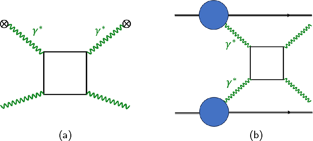
Figure 3 Two variants of Delbrück scattering involving two virtual photons, ${\gamma}^{\ast }$
. (a) Off a (static) Coulomb potential denoted by crosses. (b) Off a Lorentz boosted Coulomb potential in ultra-peripheral heavy-ion collisions.
${\gamma}^{\ast }$
. (a) Off a (static) Coulomb potential denoted by crosses. (b) Off a Lorentz boosted Coulomb potential in ultra-peripheral heavy-ion collisions.
2.2 Light-by-light scattering with lasers
At BIREF@HIBEF an intense optical laser ( ${\omega}_{\mathrm{L}}=1.55\;\mathrm{eV}$
) will be combined with the EuXFEL (which can run at different frequencies from about
${\omega}_{\mathrm{L}}=1.55\;\mathrm{eV}$
) will be combined with the EuXFEL (which can run at different frequencies from about $5$
to
$5$
to $24\;\mathrm{keV}$
, e.g., at
$24\;\mathrm{keV}$
, e.g., at ${\omega}_{\mathrm{X}}=8766\;\mathrm{eV}$
). This implies a CM energy given by the geometric mean of
${\omega}_{\mathrm{X}}=8766\;\mathrm{eV}$
). This implies a CM energy given by the geometric mean of ${\omega}_{\ast}={\left({\omega}_{\mathrm{L}}{\omega}_{\mathrm{X}}\right)}^{1/2}=116\;\mathrm{eV}$
. According to Equation (1), the QED cross-section will then be
${\omega}_{\ast}={\left({\omega}_{\mathrm{L}}{\omega}_{\mathrm{X}}\right)}^{1/2}=116\;\mathrm{eV}$
. According to Equation (1), the QED cross-section will then be $\sigma =1.81\times {10}^{-53}\;{\mathrm{cm}}^2$
. This is still fairly small, but the coherence of the optical laser background drastically enhances the amplitude by a factor proportional to the photon number.
$\sigma =1.81\times {10}^{-53}\;{\mathrm{cm}}^2$
. This is still fairly small, but the coherence of the optical laser background drastically enhances the amplitude by a factor proportional to the photon number.
The calculation of the relevant cross-section thus proceeds in two steps. Firstly, one employs a low-energy approximation by adopting the HE effective Lagrangian with a point-like four-photon vertex. Intuitively, the vacuum polarization loop can no longer be resolved as the effective theory is only valid for distances much larger than the Compton wave length. In a second step, one replaces two of the photon legs in Figure 1 by an external electromagnetic field representing the intense laser focus. The two steps are depicted in terms of Feynman diagrams in Figure 4.

Figure 4 Two-step modification of the QED 4-photon vertex (left) to the Heisenberg–Euler four-point interaction (centre) and coupling to an external field scattering (right).
Scattering off an optical laser background $F$
yields a coherent enhancement factor
$F$
yields a coherent enhancement factor ${F}^2$
in the amplitude. This factor is proportional to the photon number
${F}^2$
in the amplitude. This factor is proportional to the photon number ${N}_{\mathrm{L}}$
of the optical laser, hence analogous to the squared nuclear charge,
${N}_{\mathrm{L}}$
of the optical laser, hence analogous to the squared nuclear charge, ${Z}^2$
, in Delbrück scattering. Thus, replacing
${Z}^2$
, in Delbrück scattering. Thus, replacing ${Z}^2$
with
${Z}^2$
with ${F}^2\sim {N}_{\mathrm{L}}$
in Equation (4), the cross-section is expected to behave as follows:
${F}^2\sim {N}_{\mathrm{L}}$
in Equation (4), the cross-section is expected to behave as follows:
 $$\begin{align}\sigma \sim {\alpha}^4{N}_{\mathrm{L}}^2{\left(\frac{\omega_{\ast }}{m}\right)}^6\frac{1}{m^2}.\end{align}$$
The dimensionless constant of proportionality can be calculated from the low-energy effective field theory of QED:
 $$\begin{align}{\mathrm{\mathcal{L}}}_{\mathrm{eff}}=\mathcal{S}+{\mathrm{\mathcal{L}}}_{\mathrm{HE}}+{c}_{22}{F}_{\mu \nu}\square {F}^{\mu \nu}+\dots, \quad {\mathrm{\mathcal{L}}}_{\mathrm{HE}}={c}_1{\mathcal{S}}^2+{c}_2{\mathcal{P}}^2,\\[-18pt]\nonumber \end{align}$$
where ${\mathrm{\mathcal{L}}}_{\mathrm{HE}}$
is the celebrated HE Lagrangian[
Reference Heisenberg and Euler
4
] to the lowest order in field strengths. Its crucial ingredients are the fundamental Lorentz and gauge invariants:
${\mathrm{\mathcal{L}}}_{\mathrm{HE}}$
is the celebrated HE Lagrangian[
Reference Heisenberg and Euler
4
] to the lowest order in field strengths. Its crucial ingredients are the fundamental Lorentz and gauge invariants:
 $$\begin{align}\mathcal{S}=-\frac{1}{4}{F}_{\mu \nu}{F}^{\mu \nu}=\frac{1}{2}\left({\mathbf{E}}^2-{\mathbf{B}}^2\right),\end{align}$$
 $$\begin{align}\mathcal{P}=-\frac{1}{4}{F}_{\mu \nu}{\tilde{F}}^{\mu \nu}=\mathbf{E}\cdot \mathbf{B},\\[-19pt]\nonumber\end{align}$$
with the electromagnetic field strength tensor ${F}^{\mu \nu}={\partial}^{\mu }{A}^{\nu }-{\partial}^{\nu }{A}^{\mu }$
and its dual,
${F}^{\mu \nu}={\partial}^{\mu }{A}^{\nu }-{\partial}^{\nu }{A}^{\mu }$
and its dual, ${\tilde{F}}^{\mu}=\left(1/2\right){\varepsilon}^{\mu \nu \rho \sigma}{F}_{\rho \sigma}$
, gauge potential
${\tilde{F}}^{\mu}=\left(1/2\right){\varepsilon}^{\mu \nu \rho \sigma}{F}_{\rho \sigma}$
, gauge potential ${A}^{\mu }$
and low-energy constants
${A}^{\mu }$
and low-energy constants ${c}_1$
,
${c}_1$
, ${c}_2$
and
${c}_2$
and ${c}_{22}$
. The invariant
${c}_{22}$
. The invariant $\mathcal{S}$
is just the Maxwell Lagrangian, while
$\mathcal{S}$
is just the Maxwell Lagrangian, while ${\mathcal{S}}^2$
and
${\mathcal{S}}^2$
and ${\mathcal{P}}^2$
are the leading-order nonlinear corrections first employed in Ref. [Reference Euler and Kockel2]. The ellipsis represents corrections of higher order in both field strength[
Reference Heisenberg and Euler
4
] and derivatives[
Reference Mamaev, Mostepanenko and Eides
52
–
Reference Franchino-Viñas, García-Pérez, Mazzitelli, Vitagliano and Haimovichi
56
]. The low-energy constants are as follows:
${\mathcal{P}}^2$
are the leading-order nonlinear corrections first employed in Ref. [Reference Euler and Kockel2]. The ellipsis represents corrections of higher order in both field strength[
Reference Heisenberg and Euler
4
] and derivatives[
Reference Mamaev, Mostepanenko and Eides
52
–
Reference Franchino-Viñas, García-Pérez, Mazzitelli, Vitagliano and Haimovichi
56
]. The low-energy constants are as follows:
 $$\begin{align}{c}_1=\frac{8{\alpha}^2}{45{m}^4},\kern1em {c}_2=\frac{14{\alpha}^2}{45{m}^4},\kern1em {c}_{22}=\frac{\alpha }{60\pi {m}^2},\\[-20pt]\nonumber\end{align}$$
where the powers in $\alpha$
and
$\alpha$
and $m$
follow from vertex counting and dimensional analysis. These coefficients receive higher loop corrections that are parametrically suppressed with additional powers of
$m$
follow from vertex counting and dimensional analysis. These coefficients receive higher loop corrections that are parametrically suppressed with additional powers of $\alpha \ll 1$
. They account for higher-order vacuum polarization effects arising from the interaction of charges in the vacuum polarization loop; cf., for example, Ref. [Reference Gies and Karbstein57].
$\alpha \ll 1$
. They account for higher-order vacuum polarization effects arising from the interaction of charges in the vacuum polarization loop; cf., for example, Ref. [Reference Gies and Karbstein57].
In this context, we also emphasize that the structure of Equation (6) is generic for any nonlinear extension of classical electrodynamics that respects Lorentz covariance, U(1) gauge invariance and a charge conjugation parity symmetry. Hence, a measurement of the QED predictions in Equation (9) inherently also implies a restriction of the parameter space of other potential nonlinear extensions of classical electrodynamics in and beyond the Standard Model of particle physics.
In QED, the last constant, ${c}_{22}$
, is the weight of the leading-order linear vacuum polarization term and was already calculated by Dirac[
Reference Dirac
58
] and Heisenberg[
Reference Heisenberg
27
] in 1934. Its QED analogue, valid for all energies, implies a scale dependence, hence ‘running’, of the electric charge, which decreases with distance. Intuitively, this corresponds to charge screening caused by the virtual pair dipoles in the vacuum. This implies in turn that the vacuum can be viewed as a polarizable medium with both linear and nonlinear response to an external field. The associated response functions are given by the second derivatives of the effective Lagrangian with respect to
${c}_{22}$
, is the weight of the leading-order linear vacuum polarization term and was already calculated by Dirac[
Reference Dirac
58
] and Heisenberg[
Reference Heisenberg
27
] in 1934. Its QED analogue, valid for all energies, implies a scale dependence, hence ‘running’, of the electric charge, which decreases with distance. Intuitively, this corresponds to charge screening caused by the virtual pair dipoles in the vacuum. This implies in turn that the vacuum can be viewed as a polarizable medium with both linear and nonlinear response to an external field. The associated response functions are given by the second derivatives of the effective Lagrangian with respect to $F$
(or
$F$
(or $\mathbf{E}$
and
$\mathbf{E}$
and $\mathbf{B}$
). Focusing on the nonlinear case we can define macroscopic fields
$\mathbf{B}$
). Focusing on the nonlinear case we can define macroscopic fields $\mathbf{D}$
and
$\mathbf{D}$
and $\mathbf{H}$
as the derivatives of the Lagrangian
$\mathbf{H}$
as the derivatives of the Lagrangian ${\mathrm{\mathcal{L}}}_{\mathrm{eff}}=\mathcal{S}+{\mathrm{\mathcal{L}}}_{\mathrm{HE}}$
:
${\mathrm{\mathcal{L}}}_{\mathrm{eff}}=\mathcal{S}+{\mathrm{\mathcal{L}}}_{\mathrm{HE}}$
:
 $$\begin{align}{D}_i=\frac{\partial {\mathrm{\mathcal{L}}}_{\mathrm{eff}}}{\partial {E}_i}\equiv {\varepsilon}_{ij}{E}_j,\end{align}$$
 $$\begin{align}{H}_i=-\frac{\partial {\mathrm{\mathcal{L}}}_{\mathrm{eff}}}{\partial {B}_i}\equiv {\mu}_{ij}^{-1}{B}_j,\end{align}$$
where the (static) nonlinear response functions are the tensors[ Reference Baier and Breitenlohner 59 ]:
 $$\begin{align}{\varepsilon}_{ij}=\left(1+2{c}_1\mathcal{S}\right)\kern0.1em {\delta}_{ij}+2{c}_2\kern0.1em {B}_i{B}_j,\end{align}$$
 $$\begin{align}{\mu}_{ij}^{-1}=\left(1+2{c}_1\mathcal{S}\right)\kern0.1em {\delta}_{ij}-2{c}_2\kern0.1em {E}_i{E}_j.\\[-18pt]\nonumber\end{align}$$
These correspond to the dielectric and permeability tensors, respectively, and thus explicitly show the electric and magnetic response of the vacuum to external fields. In the words of Weisskopf[ Reference Weisskopf and Dan 60 ]: ‘When passing through electromagnetic fields, light will behave as if the vacuum had acquired a dielectric constant different from unity due to the influence of the fields.
From conventional optics, it is known that media with dielectric constant $\varepsilon$
and permeability
$\varepsilon$
and permeability $\mu$
have optical properties characterized by an index of refraction,
$\mu$
have optical properties characterized by an index of refraction, $n\equiv \sqrt{\varepsilon \mu}$
. In view of Equations (12) and (13) it must thus be possible to ascribe a nontrivial refractive index to the vacuum. This can indeed be done by studying the eigenvalues of the dielectric and permeability tensors,
$n\equiv \sqrt{\varepsilon \mu}$
. In view of Equations (12) and (13) it must thus be possible to ascribe a nontrivial refractive index to the vacuum. This can indeed be done by studying the eigenvalues of the dielectric and permeability tensors, ${\varepsilon}_{ij}$
and
${\varepsilon}_{ij}$
and ${\mu}_{ij}$
[
Reference Dittrich and Gies
37
, Reference Klein and Nigam
61
, Reference Koch
62
]. One finds that the vacuum is characterized by two nontrivial refractive indices,
${\mu}_{ij}$
[
Reference Dittrich and Gies
37
, Reference Klein and Nigam
61
, Reference Koch
62
]. One finds that the vacuum is characterized by two nontrivial refractive indices, ${n}_1$
and
${n}_1$
and ${n}_2$
, so that the vacuum acts like a birefringent medium.
${n}_2$
, so that the vacuum acts like a birefringent medium.
2.3 Vacuum birefringence
A web search for the term ‘vacuum birefringence’ dates its first appearance to the year 1964 when it appeared in the title of a paper by Klein and Nigam[ Reference Klein and Nigam 61 ] who employed the tensors in Equations (12) and (13) stemming from the low-energy HE Lagrangian. However, the vacuum refractive indices were first calculated (for arbitrary photon energies) by Toll in his unpublished PhD thesis[ Reference Toll 63 ] supervised by Wheeler. Other early and important contributions have been made by Erber[ Reference Erber 64 ] (preceding Klein and Nigam), Baier and Breitenlohner[ Reference Baier and Breitenlohner 59 ] and Narozhny[ Reference Narozhny 65 ]. The utilization of lasers was first suggested and analysed in Ref. [Reference Aleksandrov, Ansel’m and Moskalev66]. The HED-HIBEF experiment is based on the optimal scenario of combining an XFEL probe beam with an intense optical laser background. This was first suggested in Ref. [Reference Heinzl, Liesfeld, Amthor, Schwoerer, Sauerbrey and Wipf67].
To avoid confusion we recall that the term ‘vacuum birefringence’ refers to the refractive or dispersive properties of the vacuum (encoded in the real part of the refractive indices), while the term ‘vacuum dichroism’ describes its absorptive properties (encoded in the imaginary part of the refractive indices). In other words, dichroism amounts to a direction dependent absorption of probe photons, hence a reduction of probe intensity[ Reference Klein and Nigam 68 , Reference Heyl and Hernquist 69 ].
A quick way to derive the magnitude of the birefringence effect is to employ the differential cross-section in the CM frame, which for a $2\to 2$
process (with all masses equal) has the following universal form:
$2\to 2$
process (with all masses equal) has the following universal form:
 $$\begin{align}\frac{\mathrm{d}\sigma}{\mathrm{d}\Omega}=\frac{1}{64{\pi}^2}\frac{1}{s}\kern0.1em {\left|\mathfrak{M}\right|}^2\equiv {\left|f\left(\mathbf{l},{\mathbf{l}}^{\prime },\theta \right)\right|}^2.\end{align}$$
Here $\mathfrak{M}$
is the invariant amplitude depending on photon polarizations and momenta while
$\mathfrak{M}$
is the invariant amplitude depending on photon polarizations and momenta while $f$
is the scattering amplitude for momentum transfer,
$f$
is the scattering amplitude for momentum transfer, $\mathbf{l}\to {\mathbf{l}}^{\prime }$
, and scattering angle
$\mathbf{l}\to {\mathbf{l}}^{\prime }$
, and scattering angle $\theta$
. Microscopically, vacuum birefringence corresponds to forward scattering (
$\theta$
. Microscopically, vacuum birefringence corresponds to forward scattering ( $\mathbf{l}={\mathbf{l}}^{\prime }$
,
$\mathbf{l}={\mathbf{l}}^{\prime }$
, $\theta =0$
) with a polarization flip of a probe photon passing through an intense laser background. We thus assume the involvement of two laser photons with the same polarizations and four vectors, while the probe polarization flips,
$\theta =0$
) with a polarization flip of a probe photon passing through an intense laser background. We thus assume the involvement of two laser photons with the same polarizations and four vectors, while the probe polarization flips, $\varepsilon \to {\varepsilon}^{\prime }$
with
$\varepsilon \to {\varepsilon}^{\prime }$
with $\varepsilon \cdot {\varepsilon}^{\prime}=0$
. Choosing the optimal scenario of a 45° angle between probe and laser polarizations, one may use the textbook formulae in Ref. [Reference Akhiezer and Berestetskii33] to find the forward-flip amplitude
$\varepsilon \cdot {\varepsilon}^{\prime}=0$
. Choosing the optimal scenario of a 45° angle between probe and laser polarizations, one may use the textbook formulae in Ref. [Reference Akhiezer and Berestetskii33] to find the forward-flip amplitude $\mathfrak{M}(0)$
and hence the forward-scattering amplitude:
$\mathfrak{M}(0)$
and hence the forward-scattering amplitude:
 $$\begin{align}f\left(\mathbf{l},\mathbf{l},0\right)\equiv f(0)=\frac{\mathfrak{M}(0)}{8\pi \sqrt{s}}=\frac{4{\alpha}^2}{15\pi }{\left(\frac{\omega_{\ast }}{m}\right)}^3\frac{1}{m}. \end{align}$$
Another textbook formula (see e.g., Ref. [Reference Newton70], Chap. 1.5) relates the index of refraction to the forward-scattering amplitude. The flip amplitude, in particular, defines the difference of the vacuum refractive indices:
 $$\begin{align}\Delta n=\frac{2\pi {n}_{\mathrm{L}}}{\omega_{\ast}^2}f(0)=\frac{8{\alpha}^2}{15}\frac{I_{\mathrm{L}}}{m^4}.\end{align}$$
Here we have used that the laser photon density, ${n}_{\mathrm{L}}={N}_{\mathrm{L}}/V={I}_{\mathrm{L}}/{\omega}_{\ast }$
, is proportional to intensity,
${n}_{\mathrm{L}}={N}_{\mathrm{L}}/V={I}_{\mathrm{L}}/{\omega}_{\ast }$
, is proportional to intensity, ${I}_{\mathrm{L}}$
, measured in the CM system. This result is consistent with the intensity scaling that led to Equation (5) and the calculation[
Reference Narozhny
65
] of the refractive indices in terms of the vacuum polarization tensor (the covariant unification of dielectric and permeability tensors):
${I}_{\mathrm{L}}$
, measured in the CM system. This result is consistent with the intensity scaling that led to Equation (5) and the calculation[
Reference Narozhny
65
] of the refractive indices in terms of the vacuum polarization tensor (the covariant unification of dielectric and permeability tensors):
 $$\begin{align}{n}_i=1+4{c}_i{I}_{\mathrm{L}}\kern1.1em \mathrm{whence}\kern1.1em \Delta n=4\left({c}_2-{c}_1\right){I}_{\mathrm{L}}.\end{align}$$
This may be written in a more covariant way as follows. One introduces the probe four-vector $k=\omega \mathrm{\ell}$
with frequency
$k=\omega \mathrm{\ell}$
with frequency $\omega$
and a dimensionless null-vector
$\omega$
and a dimensionless null-vector $\mathrm{\ell}$
,
$\mathrm{\ell}$
, ${\mathrm{\ell}}^2=0$
. One then forms the ‘null-energy projection’[
Reference Shore
71
],
${\mathrm{\ell}}^2=0$
. One then forms the ‘null-energy projection’[
Reference Shore
71
], ${T}_{\mathrm{\ell \ell }}\equiv {\mathrm{\ell}}_{\mu }{T}^{\mu \nu}{\mathrm{\ell}}_{\nu }$
, of the Maxwell energy-momentum tensor,
${T}_{\mathrm{\ell \ell }}\equiv {\mathrm{\ell}}_{\mu }{T}^{\mu \nu}{\mathrm{\ell}}_{\nu }$
, of the Maxwell energy-momentum tensor, ${T}^{\mu \nu}={F}^{\mu \alpha}{F}_{\alpha}^{\nu }-{g}^{\mu \nu}\mathcal{S}$
, the traceless part of the squared field strength. For any field configuration,
${T}^{\mu \nu}={F}^{\mu \alpha}{F}_{\alpha}^{\nu }-{g}^{\mu \nu}\mathcal{S}$
, the traceless part of the squared field strength. For any field configuration, ${F}^{\mu \nu}$
, one can thus write the following:
${F}^{\mu \nu}$
, one can thus write the following:
 $$\begin{align}\frac{\Delta n}{T_{\mathrm{\ell \ell }}}={c}_2-{c}_1=\frac{2{\alpha}^2}{15{m}^4},\end{align}$$
which obviously just measures the difference of the leading-order low-energy constants in the HE Lagrangian. The difference $\Delta n$
in refractive indices induces an ellipticity
$\Delta n$
in refractive indices induces an ellipticity $\delta \equiv {k}_{\mathrm{X}}z\Delta n/2$
for a linearly polarized probe beam of wave number
$\delta \equiv {k}_{\mathrm{X}}z\Delta n/2$
for a linearly polarized probe beam of wave number ${k}_{\mathrm{X}}$
traversing the polarized vacuum across a distance
${k}_{\mathrm{X}}$
traversing the polarized vacuum across a distance $z$
. The experimental signature is then the flip probability:
$z$
. The experimental signature is then the flip probability:

with the Sauter–Schwinger intensity ${I}_{\mathrm{S}}={E}_{\mathrm{S}}^2={m}^4/4\pi \alpha =4.7\times {10}^{29}\kern0.1em \mathrm{W}/{\mathrm{cm}}^2$
. Equation (19) shows explicitly that an optimal scenario will maximize the target intensity
${I}_{\mathrm{S}}={E}_{\mathrm{S}}^2={m}^4/4\pi \alpha =4.7\times {10}^{29}\kern0.1em \mathrm{W}/{\mathrm{cm}}^2$
. Equation (19) shows explicitly that an optimal scenario will maximize the target intensity ${I}_{\mathrm{L}}$
and its spatial extent,
${I}_{\mathrm{L}}$
and its spatial extent, $z$
, while simultaneously minimizing the (reduced) probe wave length,
$z$
, while simultaneously minimizing the (reduced) probe wave length, ![]() [
Reference Heinzl, Liesfeld, Amthor, Schwoerer, Sauerbrey and Wipf
67
]. At HED-HIBEF this is realized by combining a high-intensity optical laser with an XFEL. A rough estimate with
[
Reference Heinzl, Liesfeld, Amthor, Schwoerer, Sauerbrey and Wipf
67
]. At HED-HIBEF this is realized by combining a high-intensity optical laser with an XFEL. A rough estimate with ${I}_{\mathrm{L}}={10}^{21}\kern0.1em \mathrm{W}/{\mathrm{cm}}^2$
,
${I}_{\mathrm{L}}={10}^{21}\kern0.1em \mathrm{W}/{\mathrm{cm}}^2$
, $z=10\;\unicode{x3bc} \mathrm{m}$
and
$z=10\;\unicode{x3bc} \mathrm{m}$
and ![]() (for
(for ${\omega}_{\mathrm{X}}=10\kern0.22em \mathrm{keV}$
) yields
${\omega}_{\mathrm{X}}=10\kern0.22em \mathrm{keV}$
) yields ${N}^{\prime }/N\approx {10}^{-12}$
. Obviously, such a minuscule flip probability demands a very high accuracy of the required polarization measurements. Indeed, the original suggestion to employ XFEL beams as a probe[
Reference Heinzl, Liesfeld, Amthor, Schwoerer, Sauerbrey and Wipf
67
] has been an incentive to improve the polarization purity of X-rays by several orders of magnitude to a current record of
${N}^{\prime }/N\approx {10}^{-12}$
. Obviously, such a minuscule flip probability demands a very high accuracy of the required polarization measurements. Indeed, the original suggestion to employ XFEL beams as a probe[
Reference Heinzl, Liesfeld, Amthor, Schwoerer, Sauerbrey and Wipf
67
] has been an incentive to improve the polarization purity of X-rays by several orders of magnitude to a current record of ${10}^{-11}$
[
Reference Schulze, Grabiger, Loetzsch, Marx-Glowna, Schmitt, Garcia, Hippler, Huang, Karbstein, Konôpková, Schlenvoigt, Schwinkendorf, Strohm, Toncian, Uschmann, Wille, Zastrau, Röhlsberger, Stöhlker, Cowan and Paulus
72
]. A topical review of the technical difficulties involved and how they are being addressed is given in Ref. [Reference Yu, Xu, Shen, Cowan and Schlenvoigt73].
${10}^{-11}$
[
Reference Schulze, Grabiger, Loetzsch, Marx-Glowna, Schmitt, Garcia, Hippler, Huang, Karbstein, Konôpková, Schlenvoigt, Schwinkendorf, Strohm, Toncian, Uschmann, Wille, Zastrau, Röhlsberger, Stöhlker, Cowan and Paulus
72
]. A topical review of the technical difficulties involved and how they are being addressed is given in Ref. [Reference Yu, Xu, Shen, Cowan and Schlenvoigt73].
2.4 Previous experiments
As early as 1929, Watson[
Reference Watson
74
] tried to measure a vacuum refractive index $n$
depending linearly on a static magnetic field,
$n$
depending linearly on a static magnetic field, $B$
. He used an interferometer to measure a small induced frequency shift, but did not find any effect and thus produced the upper bound of
$B$
. He used an interferometer to measure a small induced frequency shift, but did not find any effect and thus produced the upper bound of $\left(n-1\right)/B<4\times {10}^{-7}\kern0.1em {\mathrm{T}}^{-1}$
(in modern notation). In 1960 Jones[
Reference Jones
75
] measured the velocity of light in a magnetic field to high precision and found no deviation from its vacuum value. A year later, Erber[
Reference Erber
64
] discussed a number of settings (including Watson’s) that might allow measurement of a quadratic dependence of the vacuum refractive indices, hence a Cotton–Mouton effect[
Reference Cotton and Mouton
76
, Reference Cotton and Mouton
77
], as predicted by QED. Klein and Nigam[
Reference Klein and Nigam
61
] suggested using a static electric field inside a plane capacitor, but ruled the birefringence effect to be way too small. In 1979, Iacopini and Zavattini pointed out that one may use strong static magnetic fields and optimize the geometric factor
$\left(n-1\right)/B<4\times {10}^{-7}\kern0.1em {\mathrm{T}}^{-1}$
(in modern notation). In 1960 Jones[
Reference Jones
75
] measured the velocity of light in a magnetic field to high precision and found no deviation from its vacuum value. A year later, Erber[
Reference Erber
64
] discussed a number of settings (including Watson’s) that might allow measurement of a quadratic dependence of the vacuum refractive indices, hence a Cotton–Mouton effect[
Reference Cotton and Mouton
76
, Reference Cotton and Mouton
77
], as predicted by QED. Klein and Nigam[
Reference Klein and Nigam
61
] suggested using a static electric field inside a plane capacitor, but ruled the birefringence effect to be way too small. In 1979, Iacopini and Zavattini pointed out that one may use strong static magnetic fields and optimize the geometric factor ${\left(z/\lambda \right)}^2$
. To this end, one should propagate a stable optical laser beam through a magnetic cavity and increase the optical path length
${\left(z/\lambda \right)}^2$
. To this end, one should propagate a stable optical laser beam through a magnetic cavity and increase the optical path length $z$
through multiple reflections. This idea has been realized in the PVLAS experiment, which recently celebrated its 20th anniversary[
Reference Ejlli, Valle, Gastaldi, Messineo, Pengo, Ruoso and Zavattini
78
]. There are also a number of competing or complementary experiments, for which an overview may be found in Ref. [Reference Battesti, Beard, Böser, Bruyant, Budker, Crooker, Daw, Flambaum, Inada, Irastorza, Karbstein, Kim, Kozlov, Melhem, Phipps, Pugnat, Rikken, Rizzo, Schott, Semertzidis and Zavattini79] together with an extensive list of references. Figure 5, reproduced with permission from Ref. [Reference Ejlli, Valle, Gastaldi, Messineo, Pengo, Ruoso and Zavattini78], presents the historical evolution of the experimental results, the most recent of which are still about an order of magnitude above the QED prediction. (The error bars represent an uncertainty of one sigma.) The current best value has been reported by the PVLAS-FE experiment as follows:
$z$
through multiple reflections. This idea has been realized in the PVLAS experiment, which recently celebrated its 20th anniversary[
Reference Ejlli, Valle, Gastaldi, Messineo, Pengo, Ruoso and Zavattini
78
]. There are also a number of competing or complementary experiments, for which an overview may be found in Ref. [Reference Battesti, Beard, Böser, Bruyant, Budker, Crooker, Daw, Flambaum, Inada, Irastorza, Karbstein, Kim, Kozlov, Melhem, Phipps, Pugnat, Rikken, Rizzo, Schott, Semertzidis and Zavattini79] together with an extensive list of references. Figure 5, reproduced with permission from Ref. [Reference Ejlli, Valle, Gastaldi, Messineo, Pengo, Ruoso and Zavattini78], presents the historical evolution of the experimental results, the most recent of which are still about an order of magnitude above the QED prediction. (The error bars represent an uncertainty of one sigma.) The current best value has been reported by the PVLAS-FE experiment as follows:
 $$\begin{align}\frac{\Delta {n}^{\left(\mathrm{PVLAS}-\mathrm{FE}\right)}}{B^2}=\left(+19\pm 27\right)\times {10}^{-24}\ {\mathrm{T}}^{-2},\end{align}$$

Figure 5 Historical evolution of the results for vacuum birefringence experiments employing static magnetic fields (reproduced with permission from Ref. [Reference Ejlli, Valle, Gastaldi, Messineo, Pengo, Ruoso and Zavattini78], where more details can be found). The green horizontal line represents ${k}_{\mathrm{CMV}}\equiv {c}_2-{c}_1$
.
${k}_{\mathrm{CMV}}\equiv {c}_2-{c}_1$
.
where $B$
denotes the external static magnetic field being probed. To compare with the QED result, we note that for a static magnetic field probed at the right angle,
$B$
denotes the external static magnetic field being probed. To compare with the QED result, we note that for a static magnetic field probed at the right angle, ${T}_{\mathrm{\ell \ell }}={B}^2$
. Introducing the magnetic Sauter–Schwinger field strength,
${T}_{\mathrm{\ell \ell }}={B}^2$
. Introducing the magnetic Sauter–Schwinger field strength, ${B}_{\mathrm{S}}={m}^2/e=4.41\times {10}^9\ \mathrm{T}$
, the general result in Equation (18) leads to the following:
${B}_{\mathrm{S}}={m}^2/e=4.41\times {10}^9\ \mathrm{T}$
, the general result in Equation (18) leads to the following:
 $$\begin{align}{k}_{\mathrm{CMV}} &\equiv \frac{\Delta {n}^{\mathrm{stat}}}{B^2} ={c}_2-{c}_1=\frac{2{\alpha}^2}{15{m}^4}=\frac{\alpha }{30\pi}\frac{1}{B_{\mathrm{S}}^2} \nonumber \\ &=4\times {10}^{-24}\ {\mathrm{T}}^{-2}.\end{align}$$
This constant, containing only the basic QED parameters, has been called the Cotton–Mouton constant of the vacuum (hence the acronym CMV) in Ref. [Reference Battesti, Beard, Böser, Bruyant, Budker, Crooker, Daw, Flambaum, Inada, Irastorza, Karbstein, Kim, Kozlov, Melhem, Phipps, Pugnat, Rikken, Rizzo, Schott, Semertzidis and Zavattini79]. The same value is obtained for the HED-HIBEF scenario of probing an optical laser background, cf. Equations (16) and (18), as ${T}_{\mathrm{\ell \ell }}=4{F}^2=4{I}_{\mathrm{L}}$
(assuming a head-on collision). Hence
${T}_{\mathrm{\ell \ell }}=4{F}^2=4{I}_{\mathrm{L}}$
(assuming a head-on collision). Hence
 $$\begin{align}\frac{\Delta {n}^{\mathrm{CF}}}{4{F}^2}={c}_2-{c}_1,\end{align}$$
where CF stands for ‘crossed field’ with $F=E=B$
and
$F=E=B$
and $\mathbf{E}\cdot \mathbf{B}=0$
.
$\mathbf{E}\cdot \mathbf{B}=0$
.
Strong-field vacuum polarization effects also play an important role in astrophysics and cosmology. For instance, extreme field magnitudes can be found in the magnetosphere of neutron stars and magnetars. Several years ago it was claimed that measurements of the polarization degree of such neutron stars provide evidence for an active role of vacuum birefringence[ Reference Mignani, Testa, Caniulef, Taverna, Turolla, Zane and Wu 10 ]. The subsequent scientific debate[ Reference Capparelli, Damiano, Maiani and Polosa 80 ] highlights the necessity of a controlled laboratory verification of the effect, which in turn should provide input for improved models of neutron star environments.
Very recently the STAR collaboration has reported the observation of (linear) Breit–Wheeler pair production[
Reference Adam, Adamczyk and Adams
81
], that is, the process $\gamma +\gamma \to {e}^{+}+{e}^{-}$
. As this was realized in ultra-peripheral heavy-ion collisions, the pair production is actually proceeding via the Landau–Lifshitz process[
Reference Landau and Lifshitz
82
] at low photon virtualities; see Figure 6(a). Via the optical theorem, this process is related to Delbrück scattering as observed by the ATLAS collaboration – upon ‘cutting’ the fermion loop in Figure 3(b). It has been shown that polarization flips induced by this diagram lead to modulations in the angular pair spectra, as shown in Figure 6(b) reproduced with permission from the recent review[
Reference Brandenburg, Seger, Xu and Zha
11
]. The authors of Ref. [Reference Brandenburg, Seger, Xu and Zha11] have interpreted this as an indirect signal for vacuum birefringence.
$\gamma +\gamma \to {e}^{+}+{e}^{-}$
. As this was realized in ultra-peripheral heavy-ion collisions, the pair production is actually proceeding via the Landau–Lifshitz process[
Reference Landau and Lifshitz
82
] at low photon virtualities; see Figure 6(a). Via the optical theorem, this process is related to Delbrück scattering as observed by the ATLAS collaboration – upon ‘cutting’ the fermion loop in Figure 3(b). It has been shown that polarization flips induced by this diagram lead to modulations in the angular pair spectra, as shown in Figure 6(b) reproduced with permission from the recent review[
Reference Brandenburg, Seger, Xu and Zha
11
]. The authors of Ref. [Reference Brandenburg, Seger, Xu and Zha11] have interpreted this as an indirect signal for vacuum birefringence.

Figure 6 The STAR experiment. (a) Landau–Lifshitz process. (b) Modulation signalling vacuum birefringence by means of the optical theorem (reproduced with permission from Ref. [Reference Brandenburg, Seger, Xu and Zha11]).

Figure 7 Overview of different collision geometries: (a) the conventional head-on two-beam scenario; (b)–(e) three-beam scenarios where the XFEL is collided with two optical lasers. In (c) one of the optical beams is frequency doubled[ Reference Ahmadiniaz, Cowan, Grenzer, Franchino-Viñas, Garcia, Šmid, Toncian, Trejo and Schützhold 83 ].
3 Prospective scenarios
As detailed in the previous section, real LbL scattering has a very small cross-section. Any prospective scenario must be able to deliver a signal that can be distinguished from the noise of the background photons. At the moment, three different proposals – and viable combinations thereof – are available that constitute prospective routes towards a first measurement of the effect at HED-HIBEF. All these proposals are intimately related and look very similar at first glance. However, they differ decisively in the details and thus come with different experimental challenges. Two of these are two-beam scenarios using the collision of the XFEL with the intense ReLaX beam, and the third one summarizes three-beam scenarios requiring the XFEL to collide with two intense laser beams, generated by splitting the original ReLaX beam into two beams. (See Figure 7 for an overview of different collision geometries.) Focusing only on the essentials (see Sections 3.1–3.3 below for a detailed discussion of each of these scenarios), the two-beam scenarios are as follows.
-
(1) The conventional vacuum birefringence scenario[ Reference Heinzl, Liesfeld, Amthor, Schwoerer, Sauerbrey and Wipf 67 , Reference Schlenvoigt, Heinzl, Schramm, Cowan and Sauerbrey 84 ] that envisions the collision of the two beams in a counter-propagation geometry. It uses exclusively the polarization flip of X-ray probe photons. This small quantum vacuum signal needs to be separated from the large background of probe photons traversing the high-intensity pump focus without interaction. A key parameter for the measurement of this effect is the quality of the employed polarimeter, which is typically quantified in terms of its polarization purity $\mathcal{P}$
. This represents the fraction of background photons registered in the ideally empty, perpendicularly polarized mode[
Reference Marx, Schulze, Uschmann, Kämpfer, Lötzsch, Wehrhan, Wagner, Detlefs, Roth, Härtwig, Förster, Stöhlker and Paulus
85
]. For the XFEL and intense laser parameters attainable at HED-HIBEF the signal is found to be background dominated[
Reference Schulze, Grabiger, Loetzsch, Marx-Glowna, Schmitt, Garcia, Hippler, Huang, Karbstein, Konôpková, Schlenvoigt, Schwinkendorf, Strohm, Toncian, Uschmann, Wille, Zastrau, Röhlsberger, Stöhlker, Cowan and Paulus
72
]. However, by an appropriate choice of beam waists, the divergence of the signal can be made wider than that of the probe, such that angular cuts can be used to improve the signal-to-background ratio at the expense of reduced absolute photon numbers[
Reference King, Di Piazza and Keitel
17
, Reference King, Di Piazza and Keitel
86
–
Reference Karbstein, Gies, Reuter and Zepf
88
].
$\mathcal{P}$
. This represents the fraction of background photons registered in the ideally empty, perpendicularly polarized mode[
Reference Marx, Schulze, Uschmann, Kämpfer, Lötzsch, Wehrhan, Wagner, Detlefs, Roth, Härtwig, Förster, Stöhlker and Paulus
85
]. For the XFEL and intense laser parameters attainable at HED-HIBEF the signal is found to be background dominated[
Reference Schulze, Grabiger, Loetzsch, Marx-Glowna, Schmitt, Garcia, Hippler, Huang, Karbstein, Konôpková, Schlenvoigt, Schwinkendorf, Strohm, Toncian, Uschmann, Wille, Zastrau, Röhlsberger, Stöhlker, Cowan and Paulus
72
]. However, by an appropriate choice of beam waists, the divergence of the signal can be made wider than that of the probe, such that angular cuts can be used to improve the signal-to-background ratio at the expense of reduced absolute photon numbers[
Reference King, Di Piazza and Keitel
17
, Reference King, Di Piazza and Keitel
86
–
Reference Karbstein, Gies, Reuter and Zepf
88
]. -
(2) A dark-field approach[ Reference Karbstein, Ullmann, Mosman and Zepf 23 ] based on modifying the probe beam with a well-defined beam stop so as to exhibit a shadow in both the converging and expanding beams while retaining a peaked focus profile. This should allow access to both the parallel and perpendicular polarized components of the nonlinear vacuum response scattered into the shadow where the background is significantly reduced. In this scenario, the key parameter is the quality of the shadow, which can be quantified in terms of the unwanted background measured within the shadow. It remains to be shown that a sufficiently good shadow quality
$\mathcal{S}$
ensuring a signal-to-background ratio above unity can be realized in experiments for the XFEL and intense laser parameters available at HED-HIBEF. However, the outcome of an elementary proof-of-concept experiment at an X-ray tube[
Reference Karbstein, Ullmann, Mosman and Zepf
23
] and the results of numerical diffraction simulations performed by our collaboration look sufficiently promising that this scenario is the one we have selected to first explore experimentally; cf. also Section 4 below.


Finally, the three-beam scenarios aim at verifying quantum vacuum nonlinearity in the following.
-
(3) Four-wave-mixing processes[ Reference Lundstrom, Brodin, Lundin, Marklund, Bingham, Collier, Mendonca and Norreys 14 , Reference Lundin, Marklund, Lundstrom, Brodin, Collier, Bingham, Mendonca and Norreys 15 , Reference Ahmadiniaz, Cowan, Grenzer, Franchino-Viñas, Garcia, Šmid, Toncian, Trejo and Schützhold 83 , Reference Gies, Karbstein, Kohlfürst and Seegert 89 – Reference Berezin and Fedotov 92 ] where the XFEL is collided with two intense optical laser beams that are derived from the same source and are focused to the same spot. Since the optical beams have the same frequency and propagate in different directions, this enables a new kind of quasi-elastic scattering signal at the XFEL photon frequency, the generation of which involves the absorption of a field quantum from one of the intense beams and emission into the other. Due to the associated finite momentum transfer, this signal is scattered into a well-defined direction away from the forward direction of the XFEL. Moreover, three-beam setups can also induce sizeable signals characterized by a frequency shift. While an enlarged phase space seems beneficial, it remains to be shown that the additional challenges coming with the experimental control of three laser beams can be mastered in such a way as to benefit from the additional signal photon channels facilitated by three-beam scenarios.
For the experimental implementation of a given scenario, the central interest is in the number of X-ray signal photons that can be discerned from the typically large background of the EuXFEL beam. Only these constitute a signature of quantum vacuum nonlinearity that is detectable in an experiment. To address this theoretically, we model the near-infrared (NIR) high-intensity and XFEL beams driving the nonlinear quantum vacuum signals as paraxial solutions of the wave equation, supplemented with a Gaussian pulse envelope. In general, the electric field of a paraxial beam can be expanded as $\mathbf{E}={\mathbf{E}}^{(0)}\left(\varsigma \right)+\varsigma \kern0.1em {\mathbf{E}}^{(1)}\left(\varsigma \right)+\cdots$
, that is, in powers of the small parameter
$\mathbf{E}={\mathbf{E}}^{(0)}\left(\varsigma \right)+\varsigma \kern0.1em {\mathbf{E}}^{(1)}\left(\varsigma \right)+\cdots$
, that is, in powers of the small parameter $\varsigma ={w}_0/{z}_{\mathrm{R}}$
, where
$\varsigma ={w}_0/{z}_{\mathrm{R}}$
, where ${w}_0$
is the beam waist and
${w}_0$
is the beam waist and ${z}_{\mathrm{R}}=\omega {w}_0^2/2$
is the Rayleigh length of the fundamental Gaussian beam solution;
${z}_{\mathrm{R}}=\omega {w}_0^2/2$
is the Rayleigh length of the fundamental Gaussian beam solution; $\omega =2\pi /\lambda$
is the oscillation frequency of a beam with central wavelength
$\omega =2\pi /\lambda$
is the oscillation frequency of a beam with central wavelength $\lambda$
. Throughout this work, we truncate the paraxial expansion at leading order and use
$\lambda$
. Throughout this work, we truncate the paraxial expansion at leading order and use $\mathbf{E}\approx {\mathbf{E}}^{(0)}\left(\varsigma \right)$
. For the XFEL beam focused to waist sizes much larger than its diffraction limit this is clearly a well-justified approximation. For the high-intensity laser we only consider waists fulfilling
$\mathbf{E}\approx {\mathbf{E}}^{(0)}\left(\varsigma \right)$
. For the XFEL beam focused to waist sizes much larger than its diffraction limit this is clearly a well-justified approximation. For the high-intensity laser we only consider waists fulfilling ${w}_0\ge 1.1\kern0.22em \unicode{x3bc} \mathrm{m}$
, which translates into
${w}_0\ge 1.1\kern0.22em \unicode{x3bc} \mathrm{m}$
, which translates into $\varsigma \le 0.23$
for the employed wavelength. A good indication that the leading-order paraxial approximation is sufficiently accurate also in this case is the good agreement of the analytical estimates based exclusively on the leading-order paraxial approximation with the corresponding outcomes of a Maxwell-consistent numerical simulation demonstrated in an all-optical setup where the colliding beams are focused close to the diffraction limit[
Reference Blinne, Gies, Karbstein, Kohlfürst and Zepf
93
, Reference Schütze, Doyle, Schreiber, Zepf and Karbstein
94
]. Apart from the probe beam featuring a central shadow in the dark-field scenario, the description of which requires the superposition of several Laguerre–Gaussian or Hermite–Gaussian modes, we model all laser fields as linearly polarized fundamental Gaussian beams. For a beam propagating in a positive
$\varsigma \le 0.23$
for the employed wavelength. A good indication that the leading-order paraxial approximation is sufficiently accurate also in this case is the good agreement of the analytical estimates based exclusively on the leading-order paraxial approximation with the corresponding outcomes of a Maxwell-consistent numerical simulation demonstrated in an all-optical setup where the colliding beams are focused close to the diffraction limit[
Reference Blinne, Gies, Karbstein, Kohlfürst and Zepf
93
, Reference Schütze, Doyle, Schreiber, Zepf and Karbstein
94
]. Apart from the probe beam featuring a central shadow in the dark-field scenario, the description of which requires the superposition of several Laguerre–Gaussian or Hermite–Gaussian modes, we model all laser fields as linearly polarized fundamental Gaussian beams. For a beam propagating in a positive $z$
direction, this implies the following electric field profile:
$z$
direction, this implies the following electric field profile:
 $$\begin{align}E & ={E}_0\kern0.1em \exp \left(-{\left(\frac{t-z}{\tau /2}\right)}^2-{\left(\frac{r}{w}\right)}^2\right) \nonumber \\ &\quad \times \cos \left(\omega \left(t-z\right)-\frac{z}{z_{\mathrm{R}}}{\left(\frac{r}{w}\right)}^2+\arctan \frac{z}{z_{\mathrm{R}}}\right),\end{align}$$
where ${E}_0$
is the field amplitude,
${E}_0$
is the field amplitude, $\tau$
is the phase pulse duration,
$\tau$
is the phase pulse duration, $r=\sqrt{x^2+{y}^2}$
and
$r=\sqrt{x^2+{y}^2}$
and $w={w}_0\sqrt{1+{\left(z/{z}_{\mathrm{R}}\right)}^2}$
. This, in particular, implies that the peak intensity
$w={w}_0\sqrt{1+{\left(z/{z}_{\mathrm{R}}\right)}^2}$
. This, in particular, implies that the peak intensity ${I}_{\mathrm{peak}}$
of the optical laser pulse is related to the pulse energy
${I}_{\mathrm{peak}}$
of the optical laser pulse is related to the pulse energy $W$
via
$W$
via ${I}_{\mathrm{peak}}=8\sqrt{2/\pi}\kern0.1em W/\left(\pi {w}_0^2\tau \right)= 2 \times 10^{23}\ \mathrm{W}\ \mathrm{cm}^{-2} (W\ \mathrm{in}\ \mathrm{J}, w_0\ \mathrm{in}\ \unicode{x3bc} \mathrm{m}^{-2}, \tau\ \mathrm{in}\ \mathrm{fs}^{-1})$
. The focal width and pulse duration are related to the full-width-at-half-maximum (FWHM) parameters via
${I}_{\mathrm{peak}}=8\sqrt{2/\pi}\kern0.1em W/\left(\pi {w}_0^2\tau \right)= 2 \times 10^{23}\ \mathrm{W}\ \mathrm{cm}^{-2} (W\ \mathrm{in}\ \mathrm{J}, w_0\ \mathrm{in}\ \unicode{x3bc} \mathrm{m}^{-2}, \tau\ \mathrm{in}\ \mathrm{fs}^{-1})$
. The focal width and pulse duration are related to the full-width-at-half-maximum (FWHM) parameters via ${w}_0=0.85\kern0.22em {w}_{\mathrm{FWHM}}$
and
${w}_0=0.85\kern0.22em {w}_{\mathrm{FWHM}}$
and $\tau =1.7\kern0.22em {\tau}_{\mathrm{FWHM}}$
. Standard parameters to be available at HED-HIBEF are given in Table 2. For related activities at the Station of Extreme Light (SEL), which is currently under construction in Shanghai, China, see Refs. [Reference Shen, Bu, Xu, Xu, Ji, Li and Xu95–Reference Jin, Shen and Xu98].
$\tau =1.7\kern0.22em {\tau}_{\mathrm{FWHM}}$
. Standard parameters to be available at HED-HIBEF are given in Table 2. For related activities at the Station of Extreme Light (SEL), which is currently under construction in Shanghai, China, see Refs. [Reference Shen, Bu, Xu, Xu, Ji, Li and Xu95–Reference Jin, Shen and Xu98].
Table 2 EuXFEL and ReLaX parameters. The ReLaX focal width given here is for $f/\#$
focusing.
$f/\#$
focusing.
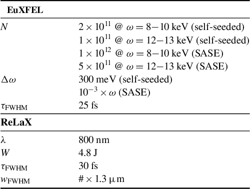
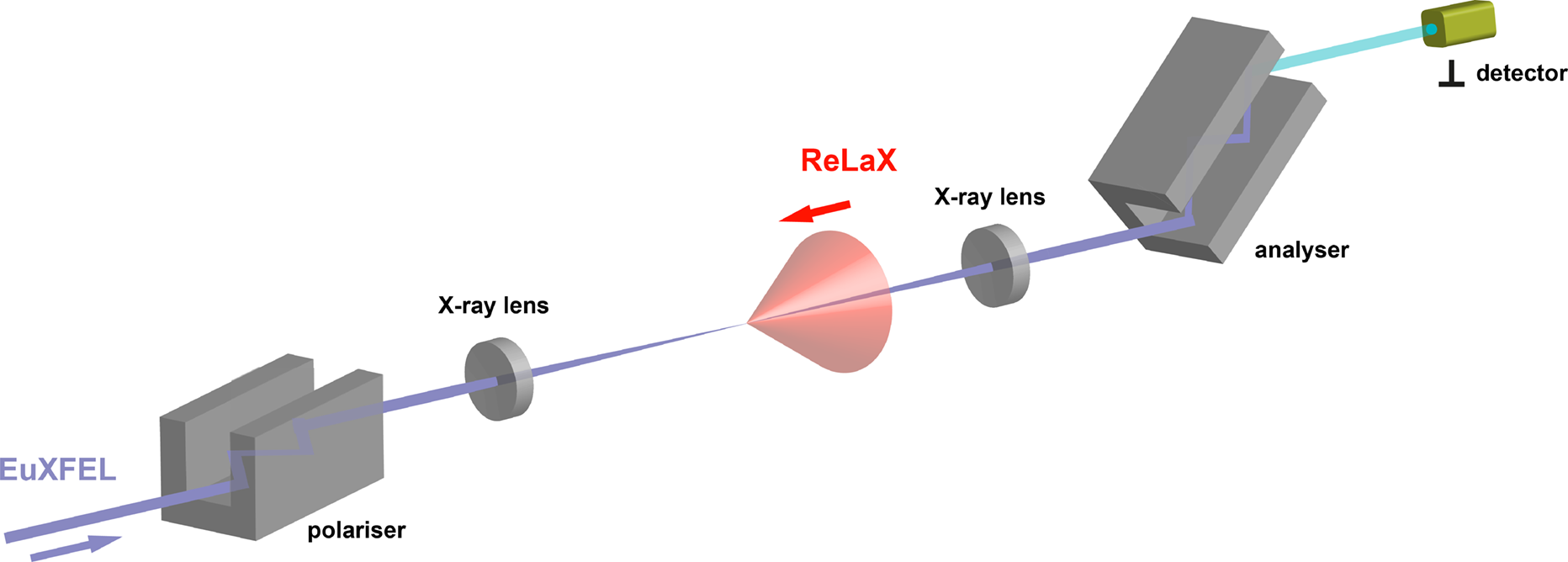
Figure 8 Schematic layout of the conventional scenario to measure vacuum birefringence. The XFEL beam is polarized with a channel-cut crystal, focused down to the interaction point with the counter-propagating high-intensity laser, recollimated and analysed with a second channel-cut crystal in a crossed position, such that only the $\perp$
-polarized component reaches the detector.
$\perp$
-polarized component reaches the detector.
3.1 Conventional two-beam scenario
The most extensively studied scenario in the present context is the conventional two-beam scenario[
Reference Aleksandrov, Ansel’m and Moskalev
66
], which envisions the head-on collision of the XFEL beam acting as probe and an NIR high-intensity pump[
Reference Heinzl, Liesfeld, Amthor, Schwoerer, Sauerbrey and Wipf
67
]. It aims at measuring the birefringence phenomenon for probe light traversing a strong electromagnetic field that arises as a direct consequence of the effective nonlinear couplings of the electromagnetic field in Equation (6). If the strong field introduces a preferred direction, such as a unidirectional magnetic field or a linearly polarized laser field, the isotropy of the vacuum is broken. In turn, the vacuum polarized by the strong field effectively features two distinct transverse propagation eigenmodes for probe light associated with different refractive indices. Correspondingly, if initially linearly polarized light (photon number $N$
) having overlap with both of these modes is sent through such a field, a small fraction
$N$
) having overlap with both of these modes is sent through such a field, a small fraction ${N}_{\perp }/N\ll 1$
of its photons are scattered into a perpendicularly polarized mode, thereby effectively supplementing it with a small ellipticity. The large photon number and the high polarization degree of XFEL beams in conjunction with the available high-purity X-ray polarimetry, reaching polarization purities down to the
${N}_{\perp }/N\ll 1$
of its photons are scattered into a perpendicularly polarized mode, thereby effectively supplementing it with a small ellipticity. The large photon number and the high polarization degree of XFEL beams in conjunction with the available high-purity X-ray polarimetry, reaching polarization purities down to the $\mathcal{P}={10}^{-11}$
level for specific photon energies in the
$\mathcal{P}={10}^{-11}$
level for specific photon energies in the $\mathcal{O}(10)\kern0.22em \mathrm{keV}$
regime[
Reference Schulze, Grabiger, Loetzsch, Marx-Glowna, Schmitt, Garcia, Hippler, Huang, Karbstein, Konôpková, Schlenvoigt, Schwinkendorf, Strohm, Toncian, Uschmann, Wille, Zastrau, Röhlsberger, Stöhlker, Cowan and Paulus
72
], make XFEL beams the ideal probe for such an experiment[
Reference Schlenvoigt, Heinzl, Schramm, Cowan and Sauerbrey
84
]. At the same time, NIR high-intensity lasers can reach the highest peak-field strengths on macroscopic scales extending over spatial distances of
$\mathcal{O}(10)\kern0.22em \mathrm{keV}$
regime[
Reference Schulze, Grabiger, Loetzsch, Marx-Glowna, Schmitt, Garcia, Hippler, Huang, Karbstein, Konôpková, Schlenvoigt, Schwinkendorf, Strohm, Toncian, Uschmann, Wille, Zastrau, Röhlsberger, Stöhlker, Cowan and Paulus
72
], make XFEL beams the ideal probe for such an experiment[
Reference Schlenvoigt, Heinzl, Schramm, Cowan and Sauerbrey
84
]. At the same time, NIR high-intensity lasers can reach the highest peak-field strengths on macroscopic scales extending over spatial distances of $\mathcal{O}(1)\kern0.22em \unicode{x3bc} \mathrm{m}$
and times of
$\mathcal{O}(1)\kern0.22em \unicode{x3bc} \mathrm{m}$
and times of $\mathcal{O}(10)\kern0.22em \mathrm{fs}$
, which are well-compatible with the characteristic scales of XFEL pulses, making them the best choice for the pump. In the collision of linearly polarized laser beams the number of polarization-flipped signal photons
$\mathcal{O}(10)\kern0.22em \mathrm{fs}$
, which are well-compatible with the characteristic scales of XFEL pulses, making them the best choice for the pump. In the collision of linearly polarized laser beams the number of polarization-flipped signal photons ${N}_{\perp }$
is maximized for a relative polarization angle of
${N}_{\perp }$
is maximized for a relative polarization angle of $\pi /4$
. As the attainable signal photon number scales with
$\pi /4$
. As the attainable signal photon number scales with ${\left(1-\cos {\vartheta}_{\mathrm{coll}}\right)}^4$
, where
${\left(1-\cos {\vartheta}_{\mathrm{coll}}\right)}^4$
, where ${\vartheta}_{\mathrm{coll}}$
is the collision angle of the two beams, the counter-propagating geometry is favoured; see Figure 8 for a schematic illustration of the experimental setup.
${\vartheta}_{\mathrm{coll}}$
is the collision angle of the two beams, the counter-propagating geometry is favoured; see Figure 8 for a schematic illustration of the experimental setup.
The most advanced theoretical modelling of this specific scenario has used pulsed paraxial beams to describe the colliding laser fields. As the smallest XFEL beam waists that have been experimentally realized so far are of the order of 100 nm[
Reference Mimura, Yumoto, Matsuyama, Koyama, Tono, Inubushi, Togashi, Sato, Kim, Fukui, Sano, Yabashi, Ohashi, Ishikawa and Yamauchi
99
], the Rayleigh lengths that can be achieved for beams with a photon energy of ${\omega}_{\mathrm{X}}=\mathcal{O}(10)\kern0.22em \mathrm{keV}$
fulfil
${\omega}_{\mathrm{X}}=\mathcal{O}(10)\kern0.22em \mathrm{keV}$
fulfil ${z}_{\mathrm{R},\mathrm{X}}\gtrsim \mathcal{O}(1)\kern0.22em \mathrm{mm}$
; cf. the definitions in the context of Equation (23) above. This value is much larger than the Rayleigh range
${z}_{\mathrm{R},\mathrm{X}}\gtrsim \mathcal{O}(1)\kern0.22em \mathrm{mm}$
; cf. the definitions in the context of Equation (23) above. This value is much larger than the Rayleigh range ${z}_{\mathrm{R},\mathrm{L}}=\mathcal{O}(10)\kern0.22em \unicode{x3bc} \mathrm{m}$
of a tightly focused NIR laser beam. It is therefore an excellent approximation to formally send
${z}_{\mathrm{R},\mathrm{L}}=\mathcal{O}(10)\kern0.22em \unicode{x3bc} \mathrm{m}$
of a tightly focused NIR laser beam. It is therefore an excellent approximation to formally send ${z}_{\mathrm{R},\mathrm{X}}\to \infty$
when determining the induced quantum vacuum signal, that is, to adopt an infinite Rayleigh length approximation[
Reference King, Di Piazza and Keitel
86
, Reference King and Keitel
87
, Reference King, Hu and Shen
90
, Reference Gies, Karbstein and Kohlfürst
100
, Reference Karbstein, Sundqvist, Schulze, Uschmann, Gies and Paulus
101
] for the probe beam. This significantly simplifies the calculation; cf. Ref. [Reference Karbstein and Oude Weernink102] for the limitations of this approximation. Modelling both laser fields as fundamental Gaussian beams at leading order in the paraxial approximation (multiplied by a Gaussian pulse envelope), the directional emission characteristics of the signal and the signal photon yield can be straightforwardly evaluated by standard computer algebra even for arbitrary collision angles and impact parameters[
Reference King and Keitel
87
, Reference Dinu, Heinzl, Ilderton, Marklund and Torgrimsson
103
, Reference Karbstein and Sundqvist
104
]; for different measurement concepts see also Refs. [Reference Ataman105, Reference Formanek, Palastro, Ramsey, Weber and Di Piazza106]. Invoking further approximations, such as the inherently very small divergence of the signal in the X-ray domain and an effective waist approximation for the pump[
Reference Karbstein
107
] (for the case of
${z}_{\mathrm{R},\mathrm{X}}\to \infty$
when determining the induced quantum vacuum signal, that is, to adopt an infinite Rayleigh length approximation[
Reference King, Di Piazza and Keitel
86
, Reference King and Keitel
87
, Reference King, Hu and Shen
90
, Reference Gies, Karbstein and Kohlfürst
100
, Reference Karbstein, Sundqvist, Schulze, Uschmann, Gies and Paulus
101
] for the probe beam. This significantly simplifies the calculation; cf. Ref. [Reference Karbstein and Oude Weernink102] for the limitations of this approximation. Modelling both laser fields as fundamental Gaussian beams at leading order in the paraxial approximation (multiplied by a Gaussian pulse envelope), the directional emission characteristics of the signal and the signal photon yield can be straightforwardly evaluated by standard computer algebra even for arbitrary collision angles and impact parameters[
Reference King and Keitel
87
, Reference Dinu, Heinzl, Ilderton, Marklund and Torgrimsson
103
, Reference Karbstein and Sundqvist
104
]; for different measurement concepts see also Refs. [Reference Ataman105, Reference Formanek, Palastro, Ramsey, Weber and Di Piazza106]. Invoking further approximations, such as the inherently very small divergence of the signal in the X-ray domain and an effective waist approximation for the pump[
Reference Karbstein
107
] (for the case of ${\vartheta}_{\mathrm{coll}}=\pi$
), one obtains rather compact analytical scaling laws describing the dependence of the signal on the various parameters of the driving laser fields. Using these scaling laws, one can quickly assess the effects of varying the characteristic parameters and thus identify promising parameter regimes prior to performing large-scale numerical simulations; cf. also the discussion below.
${\vartheta}_{\mathrm{coll}}=\pi$
), one obtains rather compact analytical scaling laws describing the dependence of the signal on the various parameters of the driving laser fields. Using these scaling laws, one can quickly assess the effects of varying the characteristic parameters and thus identify promising parameter regimes prior to performing large-scale numerical simulations; cf. also the discussion below.
For a relative polarization of $\pi /4$
between the colliding beams, the attainable number of polarization-flipped signal photons per shot can then be approximately expressed as follows[
Reference Karbstein
107
, Reference Mosman and Karbstein
108
]:
$\pi /4$
between the colliding beams, the attainable number of polarization-flipped signal photons per shot can then be approximately expressed as follows[
Reference Karbstein
107
, Reference Mosman and Karbstein
108
]:
 $$\begin{align} &{N}_{\perp} ={N}_{\mathrm{X}}\sqrt{\frac{3}{\pi }}\frac{{\left({c}_1-{c}_2\right)}^2{m}^8}{\pi }{\left(\frac{W_{\mathrm{L}}}{m}\frac{\omega_{\mathrm{X}}}{m}\right)}^2{\left(\frac{\lambda_{\mathrm{e}}}{w_{0,\mathrm{L}}}\right)}^4 \nonumber \\& \times \sqrt{g(0)g\left(\frac{w_{0,\mathrm{X}}}{w_{0,\mathrm{L}}}\right)}\exp \left(\! -2{\left(\frac{r_0}{w_{0,\mathrm{X}}}\right)}^2\left(\! 1-\sqrt{\frac{g\left(\!\frac{w_{0,\mathrm{X}}}{w_{0,\mathrm{L}}}\right)}{g(0)}}\right) \!\right)\! ,\end{align}$$
where ${c}_1$
and
${c}_1$
and ${c}_2$
are the low-energy constants introduced in Equation (9),
${c}_2$
are the low-energy constants introduced in Equation (9), ${W}_{\mathrm{L}}$
is the laser pulse energy of the pump,
${W}_{\mathrm{L}}$
is the laser pulse energy of the pump, ${w}_0$
denotes the beam waist,
${w}_0$
denotes the beam waist, ${r}_0$
is the transverse impact parameter and we used the shorthand notation:
${r}_0$
is the transverse impact parameter and we used the shorthand notation:
 $$\begin{align} & g(b):= \frac{1}{{\left(1+2{b}^2\right)}^2}\kern0.1em \nonumber \\ &\quad \times F\left(\frac{4{z}_{\mathrm{R},\mathrm{L}}\sqrt{1+2{b}^2}}{\sqrt{\tau_{\mathrm{X}}^2+{\tau}_{\mathrm{L}}^2/2}},\frac{2\left({z}_0-{t}_0\right)}{\sqrt{\tau_{\mathrm{X}}^2+{\tau}_{\mathrm{L}}^2/2}},\frac{\tau_{\mathrm{X}}}{\tau_{\mathrm{L}}}\right),\kern1em \mathrm{with} \nonumber\\ {} & F\left(\chi, {\chi}_0,\rho \right):= \sqrt{\frac{1+2{\rho}^2}{3}}\kern0.1em {\chi}^2\kern0.1em {\mathrm{e}}^{2\left({\chi}^2-{\chi}_0^2\right)}{\int}_{-\infty}^{\infty}\mathrm{d}K\kern0.1em {\mathrm{e}}^{-{K}^2}\kern0.1em \nonumber \\ &\quad \times {\left|\sum \limits_{s=\pm 1}{\mathrm{e}}^{2s\left(\rho K-i{\chi}_0\right)\chi}\kern0.1em \operatorname{erfc}\left(s\left(\rho K-i{\chi}_0\right)+\chi \right)\right|}^2.\end{align}$$
The entire dependence of Equation (24) on the longitudinal beam parameters, namely the Rayleigh length of the pump ${z}_{\mathrm{R},\mathrm{L}}$
, the
${z}_{\mathrm{R},\mathrm{L}}$
, the $1/{\mathrm{e}}^2$
pulse durations
$1/{\mathrm{e}}^2$
pulse durations ${\tau}_{\mathrm{X}}$
,
${\tau}_{\mathrm{X}}$
, ${\tau}_{\mathrm{L}}$
and the spatiotemporal offset
${\tau}_{\mathrm{L}}$
and the spatiotemporal offset ${z}_0-{t}_0$
between the probe and pump foci in longitudinal direction, is encoded in the function
${z}_0-{t}_0$
between the probe and pump foci in longitudinal direction, is encoded in the function $g(b)$
defined in Equation (25). Note that in the limit of
$g(b)$
defined in Equation (25). Note that in the limit of ${w}_{0,\mathrm{X}}\ll {w}_{0,\mathrm{L}}$
and
${w}_{0,\mathrm{X}}\ll {w}_{0,\mathrm{L}}$
and $\left\{{\tau}_{\mathrm{X}},{\tau}_{\mathrm{L}}\right\}\gg {z}_{\mathrm{R},\mathrm{L}}$
we have
$\left\{{\tau}_{\mathrm{X}},{\tau}_{\mathrm{L}}\right\}\gg {z}_{\mathrm{R},\mathrm{L}}$
we have $g(b)\sim {\left({z}_{\mathrm{R},\mathrm{L}}/{\tau}_{\mathrm{L}}\right)}^2$
[
Reference Karbstein
107
], and the form of Equation (19) with characteristic distance
$g(b)\sim {\left({z}_{\mathrm{R},\mathrm{L}}/{\tau}_{\mathrm{L}}\right)}^2$
[
Reference Karbstein
107
], and the form of Equation (19) with characteristic distance $z\sim {z}_{\mathrm{R},\mathrm{L}}$
is recovered. The dependence of the signal on the impact parameter
$z\sim {z}_{\mathrm{R},\mathrm{L}}$
is recovered. The dependence of the signal on the impact parameter ${r}_0$
is particularly relevant, as experiments have shown that focusing leads to an inevitable beam jitter characterized by spatial fluctuations of the order of the beam waist, that is,
${r}_0$
is particularly relevant, as experiments have shown that focusing leads to an inevitable beam jitter characterized by spatial fluctuations of the order of the beam waist, that is, ${r}_0\sim {w}_{0,\mathrm{L}}$
. Another important signal parameter is the
${r}_0\sim {w}_{0,\mathrm{L}}$
. Another important signal parameter is the $1/{\mathrm{e}}^2$
radial divergence:
$1/{\mathrm{e}}^2$
radial divergence:
 $$\begin{align}{\theta}_{\mathrm{signal}}={\theta}_{\mathrm{X}}\kern0.1em {\left(\frac{g\left(\frac{w_{0,\mathrm{X}}}{w_{0,\mathrm{L}}}\right)}{g(0)}\right)}^{-\frac{1}{4}},\end{align}$$
where ${\theta}_{\mathrm{X}}=2/\left({\omega}_{\mathrm{X}}{w}_{0,\mathrm{X}}\right)$
is the radial divergence of the probe beam, and thus also the divergence of the background
${\theta}_{\mathrm{X}}=2/\left({\omega}_{\mathrm{X}}{w}_{0,\mathrm{X}}\right)$
is the radial divergence of the probe beam, and thus also the divergence of the background ${N}_{\perp, \mathrm{bgr}}\sim \mathcal{P}{N}_{\mathrm{X}}$
to be registered at the detector.
${N}_{\perp, \mathrm{bgr}}\sim \mathcal{P}{N}_{\mathrm{X}}$
to be registered at the detector.
Equation (24) predicts the maximum value of ${N}_{\perp }$
for optimal collisions (
${N}_{\perp }$
for optimal collisions ( ${r}_0={z}_0={t}_0=0$
) and other fixed parameters to be reached for small probe waists,
${r}_0={z}_0={t}_0=0$
) and other fixed parameters to be reached for small probe waists, ${w}_{0,\mathrm{X}}\ll {w}_{0,\mathrm{L}}$
. In this case, one obtains the polarization-flip counts
${w}_{0,\mathrm{X}}\ll {w}_{0,\mathrm{L}}$
. In this case, one obtains the polarization-flip counts
 $$\begin{align}{\displaystyle \begin{array}{c||c|c}f/\#& f/1& f/2\\\hline {}{N}_{\perp }& 0.044& 0.0045\end{array}},\end{align}$$
for an XFEL energy of ${\omega}_{\mathrm{X}}=9835\kern0.1em \mathrm{eV}$
and the standard self-seeding parameters in Table 2 with
${\omega}_{\mathrm{X}}=9835\kern0.1em \mathrm{eV}$
and the standard self-seeding parameters in Table 2 with $f/1$
(
$f/1$
( $f/2$
) focusing. Self-seeding is the option of choice for experiments aiming at the detection of polarization-flip signals, as the probe bandwidth
$f/2$
) focusing. Self-seeding is the option of choice for experiments aiming at the detection of polarization-flip signals, as the probe bandwidth $\Delta \omega$
is of the same order as the quite narrow acceptance bandwidth of crystal polarimeters. In contrast, the self-amplified spontaneous emission (SASE) bandwidth is typically much larger; cf. Table 2. In the determination of
$\Delta \omega$
is of the same order as the quite narrow acceptance bandwidth of crystal polarimeters. In contrast, the self-amplified spontaneous emission (SASE) bandwidth is typically much larger; cf. Table 2. In the determination of ${N}_{\perp }$
we also took into account that the quasi-channel-cut (QCC) crystal acting as polarizer increases the probe pulse duration from its original value given in Table 2 to
${N}_{\perp }$
we also took into account that the quasi-channel-cut (QCC) crystal acting as polarizer increases the probe pulse duration from its original value given in Table 2 to ${\tau}_{\mathrm{FWHM}}=50\kern0.22em \mathrm{fs}$
[
Reference Karbstein, Sundqvist, Schulze, Uschmann, Gies and Paulus
101
]. Using
${\tau}_{\mathrm{FWHM}}=50\kern0.22em \mathrm{fs}$
[
Reference Karbstein, Sundqvist, Schulze, Uschmann, Gies and Paulus
101
]. Using $\mathcal{P}={10}^{-11}$
[
Reference Schulze, Grabiger, Loetzsch, Marx-Glowna, Schmitt, Garcia, Hippler, Huang, Karbstein, Konôpková, Schlenvoigt, Schwinkendorf, Strohm, Toncian, Uschmann, Wille, Zastrau, Röhlsberger, Stöhlker, Cowan and Paulus
72
] and neglecting real-world imperfections (such as inevitable losses coming with the lenses used for focusing), the values in Equation (27) imply the associated signal-to-background ratios to be given by the following:
$\mathcal{P}={10}^{-11}$
[
Reference Schulze, Grabiger, Loetzsch, Marx-Glowna, Schmitt, Garcia, Hippler, Huang, Karbstein, Konôpková, Schlenvoigt, Schwinkendorf, Strohm, Toncian, Uschmann, Wille, Zastrau, Röhlsberger, Stöhlker, Cowan and Paulus
72
] and neglecting real-world imperfections (such as inevitable losses coming with the lenses used for focusing), the values in Equation (27) imply the associated signal-to-background ratios to be given by the following:
 $$\begin{align}{\displaystyle \begin{array}{c||c|c}f/\#& f/1& f/2\\\hline {}{N}_{\perp }/\left(\mathcal{P}{N}_{\mathrm{X}}\right)& 0.022& 0.0023\end{array}}.\end{align}$$
These values are less than unity so the signal is background dominated. Moreover, in the limit considered, we have ${\theta}_{\mathrm{signal}}\approx {\theta}_{\mathrm{X}}$
, and the dependence of the signal on the impact parameter
${\theta}_{\mathrm{signal}}\approx {\theta}_{\mathrm{X}}$
, and the dependence of the signal on the impact parameter ${r}_0$
simplifies to
${r}_0$
simplifies to ${N}_{\perp}\sim \exp (-2{({r}_0/{w}_{0,\mathrm{L}})}^2)$
.
${N}_{\perp}\sim \exp (-2{({r}_0/{w}_{0,\mathrm{L}})}^2)$
.
On the other hand, for matching waists, ${w}_{0,\mathrm{X}}={w}_{0,\mathrm{L}}$
, the signal is reduced by roughly a factor of three to
${w}_{0,\mathrm{X}}={w}_{0,\mathrm{L}}$
, the signal is reduced by roughly a factor of three to ${N}_{\perp}\simeq 0.017$
(
${N}_{\perp}\simeq 0.017$
( $0.0015$
) for
$0.0015$
) for $f/1$
(
$f/1$
( $f/2$
) focusing. At the same time the divergence of the signal,
$f/2$
) focusing. At the same time the divergence of the signal, ${\theta}_{\mathrm{signal}}\approx 1.6\kern0.1em {\theta}_{\mathrm{X}}$
, becomes wider than that of the probe. This can be intuitively understood as follows: for a counter-propagating geometry the transverse extent of the strong-field interaction region is effectively determined by the transverse profile of the product
${\theta}_{\mathrm{signal}}\approx 1.6\kern0.1em {\theta}_{\mathrm{X}}$
, becomes wider than that of the probe. This can be intuitively understood as follows: for a counter-propagating geometry the transverse extent of the strong-field interaction region is effectively determined by the transverse profile of the product ${\mathrm{\mathcal{E}}}_{\mathrm{X}}(x)\kern0.1em {\mathrm{\mathcal{E}}}_{\mathrm{L}}^2(x)$
of the focus field profiles of the probe and pump, the Fourier transform of which governs the far-field distribution of the signal. When
${\mathrm{\mathcal{E}}}_{\mathrm{X}}(x)\kern0.1em {\mathrm{\mathcal{E}}}_{\mathrm{L}}^2(x)$
of the focus field profiles of the probe and pump, the Fourier transform of which governs the far-field distribution of the signal. When ${w}_{0,\mathrm{X}}\gtrsim {w}_{0,\mathrm{L}}/\sqrt{2}$
, the transverse extent of the signal emission region is smaller than the focal spot of the probe, and in turn
${w}_{0,\mathrm{X}}\gtrsim {w}_{0,\mathrm{L}}/\sqrt{2}$
, the transverse extent of the signal emission region is smaller than the focal spot of the probe, and in turn ${\theta}_{\mathrm{signal}}>{\theta}_{\mathrm{X}}$
; the factor of
${\theta}_{\mathrm{signal}}>{\theta}_{\mathrm{X}}$
; the factor of $\sqrt{2}$
is due to the linear (quadratic) dependency on the probe (pump) profile. Furthermore, as
$\sqrt{2}$
is due to the linear (quadratic) dependency on the probe (pump) profile. Furthermore, as ${N}_{\perp}\sim \exp \left(-1.2{({r}_0/{w}_{0,\mathrm{L}})}^2\right)$
for
${N}_{\perp}\sim \exp \left(-1.2{({r}_0/{w}_{0,\mathrm{L}})}^2\right)$
for $f/1$
focusing, the dependence on
$f/1$
focusing, the dependence on ${r}_0$
– and thus the sensitivity to beam jitter in the experiment – becomes milder. Clearly, when
${r}_0$
– and thus the sensitivity to beam jitter in the experiment – becomes milder. Clearly, when ${\theta}_{\mathrm{sig}}>{\theta}_{\mathrm{X}}$
, a measurement of the full signal requires collecting photons scattered outside the forward cone of the probe on the detector. However, as
${\theta}_{\mathrm{sig}}>{\theta}_{\mathrm{X}}$
, a measurement of the full signal requires collecting photons scattered outside the forward cone of the probe on the detector. However, as ${\theta}_{\mathrm{X}}\sim 1/{w}_{0,\mathrm{X}}$
, the most tightly focused probes make the highest demands on the diameter of the collection optics.
${\theta}_{\mathrm{X}}\sim 1/{w}_{0,\mathrm{X}}$
, the most tightly focused probes make the highest demands on the diameter of the collection optics.
The above simple comparison of just two different focusing options for the probe clearly illustrates that assessing the best choice of parameters for a feasible vacuum birefringence experiment is a nontrivial task. We emphasize that improved modelling accounting for the details of the laser fields actually available in experiments will become computationally demanding and challenging.
The possibility of achieving ${\theta}_{\mathrm{sig}}>{\theta}_{\mathrm{X}}$
suggests that angular cuts can be used to improve the signal-to-background ratio in experiments: collecting only those photons scattered outside a minimum diffraction angle
${\theta}_{\mathrm{sig}}>{\theta}_{\mathrm{X}}$
suggests that angular cuts can be used to improve the signal-to-background ratio in experiments: collecting only those photons scattered outside a minimum diffraction angle ${\vartheta}_{\mathrm{min}}$
, the signal-to-background ratio can be enhanced to
${\vartheta}_{\mathrm{min}}$
, the signal-to-background ratio can be enhanced to ${\left.{N}_{\perp }/\left(\mathcal{P}{N}_{\mathrm{X}}\right)\right|}_{\vartheta >{\vartheta}_{\mathrm{min}}}>1$
at the expense of reduced absolute photon numbers. Following this route, it is even possible to achieve
${\left.{N}_{\perp }/\left(\mathcal{P}{N}_{\mathrm{X}}\right)\right|}_{\vartheta >{\vartheta}_{\mathrm{min}}}>1$
at the expense of reduced absolute photon numbers. Following this route, it is even possible to achieve ${\left.{N}_{\parallel }/{N}_{\mathrm{X}}\right|}_{\vartheta >{\vartheta}_{\mathrm{min}}}>1$
, such that one can hope to also measure the
${\left.{N}_{\parallel }/{N}_{\mathrm{X}}\right|}_{\vartheta >{\vartheta}_{\mathrm{min}}}>1$
, such that one can hope to also measure the $\parallel$
-polarized signal component[
Reference Inada, Yamazaki, Yamaji, Seino, Fan, Kamioka, Namba and Asai
44
, Reference Karbstein and Mosman
109
]. However, an experimental implementation of such a diffraction-assisted measurement concept[
Reference King, Di Piazza and Keitel
17
, Reference King and Keitel
87
] requires that any unwanted background, for example, stray light from the lenses used for focusing, can be controlled and inhibited from reaching the detector; cf. Ref. [Reference Doyle, Khademi, Hilz, Sävert, Schäfer, Schreiber and Zepf110] for a related background study at optical frequencies. This would necessitate setting up a dedicated filtering and imaging system along the lines outlined in Section 4 for the dark-field scenario.
$\parallel$
-polarized signal component[
Reference Inada, Yamazaki, Yamaji, Seino, Fan, Kamioka, Namba and Asai
44
, Reference Karbstein and Mosman
109
]. However, an experimental implementation of such a diffraction-assisted measurement concept[
Reference King, Di Piazza and Keitel
17
, Reference King and Keitel
87
] requires that any unwanted background, for example, stray light from the lenses used for focusing, can be controlled and inhibited from reaching the detector; cf. Ref. [Reference Doyle, Khademi, Hilz, Sävert, Schäfer, Schreiber and Zepf110] for a related background study at optical frequencies. This would necessitate setting up a dedicated filtering and imaging system along the lines outlined in Section 4 for the dark-field scenario.
Finally, with regard to an actual experimental implementation we need to account for several non-ideal effects associated with the optical system: (i) in experiments each reflection at a diamond surface of the QCC polarizer and analyser comes with a reduction of the number of photons by about $2\%$
[
Reference Karbstein, Sundqvist, Schulze, Uschmann, Gies and Paulus
101
] (the setup in Figure 8 employs eight reflections in total); (ii) the transmission of lenses preserving the polarization purity can be estimated as
$2\%$
[
Reference Karbstein, Sundqvist, Schulze, Uschmann, Gies and Paulus
101
] (the setup in Figure 8 employs eight reflections in total); (ii) the transmission of lenses preserving the polarization purity can be estimated as $25\%$
; (iii) the acceptance bandwidth of the polarizer,
$25\%$
; (iii) the acceptance bandwidth of the polarizer, $\Delta {\omega}_{\mathrm{diamond}}^{400}=80\kern0.22em \mathrm{meV}$
, entails a reduction of its throughput by
$\Delta {\omega}_{\mathrm{diamond}}^{400}=80\kern0.22em \mathrm{meV}$
, entails a reduction of its throughput by $\Delta {\omega}_{\mathrm{diamond}}^{400}/\Delta \omega =80/300$
for self-seeding. In consequence, both the signal and background photon numbers,
$\Delta {\omega}_{\mathrm{diamond}}^{400}/\Delta \omega =80/300$
for self-seeding. In consequence, both the signal and background photon numbers, ${N}_{\perp }$
and
${N}_{\perp }$
and $\mathcal{P}{N}_{\mathrm{X}}$
, respectively, are reduced by a factor of
$\mathcal{P}{N}_{\mathrm{X}}$
, respectively, are reduced by a factor of ${(0.98)}^8\times {(0.25)}^2\times 80/300\simeq 0.014$
from their ideal theoretical values stated in Equation (27) above.
${(0.98)}^8\times {(0.25)}^2\times 80/300\simeq 0.014$
from their ideal theoretical values stated in Equation (27) above.
While this keeps the signal-to-background ratios ${N}_{\perp }/$ $(\mathcal{P}{N}_{\mathrm{X}})$
given in Equation (28) unaltered, it results in quite a drastic reduction of the signal photon numbers attainable per shot. In particular, the best value attainable for
$(\mathcal{P}{N}_{\mathrm{X}})$
given in Equation (28) unaltered, it results in quite a drastic reduction of the signal photon numbers attainable per shot. In particular, the best value attainable for ${w}_{0,\mathrm{X}}\ll {w}_{0,\mathrm{L}}$
then gives rise to just
${w}_{0,\mathrm{X}}\ll {w}_{0,\mathrm{L}}$
then gives rise to just ${N}_{\perp}\simeq 6.2\times {10}^{-4}$
(
${N}_{\perp}\simeq 6.2\times {10}^{-4}$
( $6.4\times {10}^{-5}$
) polarization-flipped signal photons per shot reaching the detector for
$6.4\times {10}^{-5}$
) polarization-flipped signal photons per shot reaching the detector for $f/1$
(
$f/1$
( $f/2$
) focusing. Assuming Poissonian statistics,
$f/2$
) focusing. Assuming Poissonian statistics,
 $$\begin{align} n & {>\#}^2\kern0.1em \frac{1}{2}{\left(\left({N}_{\mathrm{sig}}+{N}_{\mathrm{bgr}}\right)\ln \left(1+\frac{N_{\mathrm{sig}}}{N_{\mathrm{bgr}}}\right)-{N}_{\mathrm{sig}}\right)}^{-1} \nonumber \\& {=\#}^2\kern0.1em \frac{N_{\mathrm{bgr}}}{N_{\mathrm{sig}}^2}\left(1+\mathcal{O}\left(\frac{N_{\mathrm{sig}}}{N_{\mathrm{bgr}}}\right)\right)\end{align}$$
shots are required for a measurement with a significance of $\#\sigma$
[
Reference Cowan
111
], where
$\#\sigma$
[
Reference Cowan
111
], where ${N}_{\mathrm{sig}}$
and
${N}_{\mathrm{sig}}$
and ${N}_{\mathrm{bgr}}$
are the number of signal and background events, respectively. This implies that
${N}_{\mathrm{bgr}}$
are the number of signal and background events, respectively. This implies that $n{>\#}^2\times 7.5\times {10}^4$
(
$n{>\#}^2\times 7.5\times {10}^4$
( ${\#}^2\times 6.9\times {10}^6$
) optimal shots are required for a
${\#}^2\times 6.9\times {10}^6$
) optimal shots are required for a $\#\sigma$
confirmation of the vacuum birefringence signal with the presently available parameters at HED-HIBEF and
$\#\sigma$
confirmation of the vacuum birefringence signal with the presently available parameters at HED-HIBEF and $f/1$
(
$f/1$
( $f/2$
) focusing. Given a repetition rate of 1 Hz, this translates into the requirement of more than
$f/2$
) focusing. Given a repetition rate of 1 Hz, this translates into the requirement of more than ${\#}^2\times 21\kern0.22em \mathrm{h}$
(
${\#}^2\times 21\kern0.22em \mathrm{h}$
( ${\#}^2\times 80\kern0.22em \mathrm{days}$
) optimal shots with zero spatiotemporal offset. Lasers such as ReLaX can operate for long periods continuously. The total number of full power shots on the gratings and optics easily allow for continuous shooting on a month scale. We also note that if pointing and timing stabilization is implemented, the jitter of ReLaX can be reduced to less than the temporal and spatial sigma. In these circumstances, jitter does not materially affect the overall estimate relative to other uncertainties, such as shot-to-shot XFEL performance in seeded mode.
${\#}^2\times 80\kern0.22em \mathrm{days}$
) optimal shots with zero spatiotemporal offset. Lasers such as ReLaX can operate for long periods continuously. The total number of full power shots on the gratings and optics easily allow for continuous shooting on a month scale. We also note that if pointing and timing stabilization is implemented, the jitter of ReLaX can be reduced to less than the temporal and spatial sigma. In these circumstances, jitter does not materially affect the overall estimate relative to other uncertainties, such as shot-to-shot XFEL performance in seeded mode.
3.2 Dark-field scenario
A prospective variation of the conventional two-beam scenario detailed in Section 3.1 envisions modifying the probe beam so as to feature a shadow, or equivalently a dark field, in the converging and expanding beam while retaining a central intensity peak in the focus where it is collided with the counter-propagating high-intensity pump[ Reference Karbstein, Ullmann, Mosman and Zepf 23 , Reference Karbstein and Mosman 112 ]. In the experiment the shadow in the probe beam is generated by a well-defined beamstop inserted into the incident beam; see Figure 9 for an illustration. To demonstrate the underlying principle, we focus here on the case of a circularly symmetric shadow imprinted in the incident probe beam. Experimentally, this annular beam approach was pioneered in Refs. [Reference Peatross, Chaloupka and Meyerhofer113, Reference Zepf, Tsakiris, Pretzler, Watts, Chambers, Norreys, Andiel, Dangor, Eidmann, Gahn, Machacek, Wark and Witte114] for the detection of weak nonlinear optics signals driven by high-intensity lasers. By construction, the background is substantially reduced in the dark field, so that it may even be possible to access both polarization components of the nonlinear vacuum response. To this end, the shadow in the probe beam is to be imaged onto a polarization-sensitive detector employing an advanced filtering and imaging system. This will consist of appropriately designed and placed beamstops and apertures so as to prevent any unwanted background from reaching the detector together with the signal. We quantify the background scattered into the dark field by the shadow quality
 $$\begin{align}\mathcal{S}=\frac{1}{N_{\mathrm{X}}}{\int}_{A_{\mathrm{d}\mathrm{et}}}{\mathrm{d}}^2x\kern0.1em \frac{{\mathrm{d}}^2{N}_{\mathrm{X}}\left(x,y\right)}{\mathrm{d}x\kern0.1em \mathrm{d}y}\end{align}$$
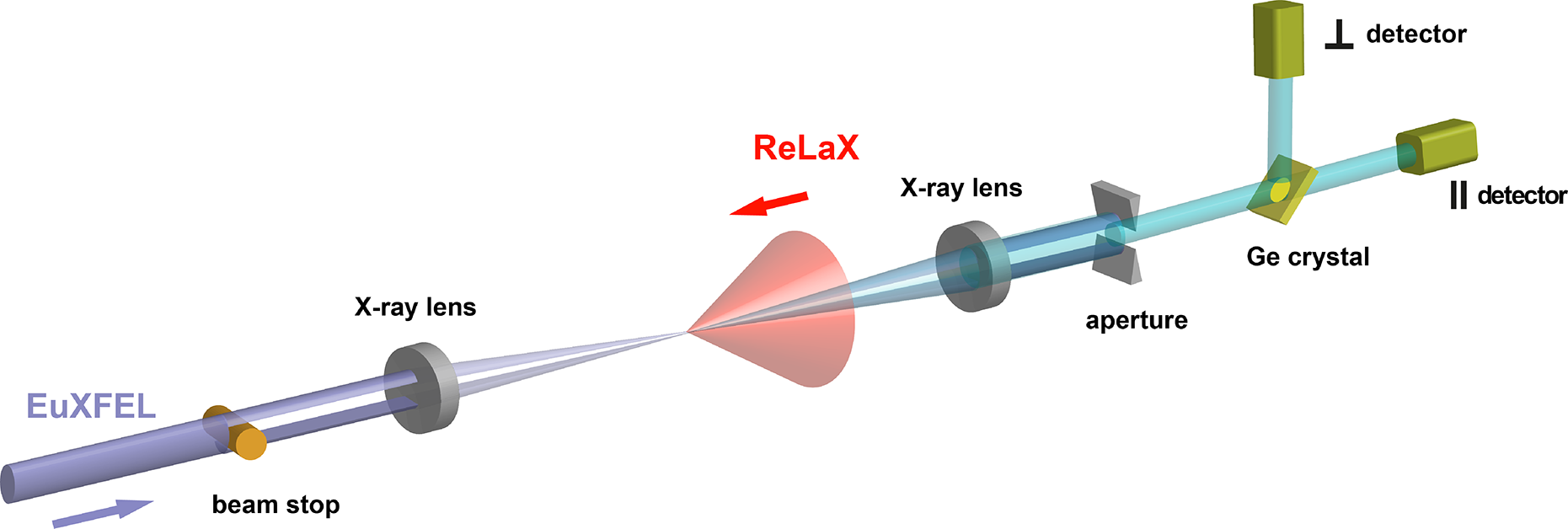
Figure 9 Schematic layout of the dark-field scenario. The XFEL is focused with a beamstop creating a shadow in the converging (expanding) beam before (after) focus while retaining a central intensity peak in the focus where it collides with a counter-propagating high-intensity pump. X-ray optics image the beamstop to a matched aperture plane. The effective interaction with the pump is strongly localized and limited to the vicinity of the probe focus. Hence, given that the overlap factor ${\mathrm{\mathcal{E}}}_{\mathrm{X}}(x){\mathrm{\mathcal{E}}}_{\mathrm{L}}^2(x)$
is sufficiently similar to that in the conventional scenario in Figure 8, a scattering signal is induced in the shadow. A crystal polarizer directs its different polarization components to separate detectors.
${\mathrm{\mathcal{E}}}_{\mathrm{X}}(x){\mathrm{\mathcal{E}}}_{\mathrm{L}}^2(x)$
is sufficiently similar to that in the conventional scenario in Figure 8, a scattering signal is induced in the shadow. A crystal polarizer directs its different polarization components to separate detectors.
that measures the fraction of the total number of input probe photons ${N}_{\mathrm{X}}$
registered by a detector of acceptance area
${N}_{\mathrm{X}}$
registered by a detector of acceptance area ${A}_{\mathrm{det}}$
in the shadow in the absence of a quantum vacuum signal, that is, for a vanishing pump field. In a theoretically idealized calculation using ideal flat-top far-field profiles and neglecting diffraction at the obstacles and apertures put into the beam path, we have
${A}_{\mathrm{det}}$
in the shadow in the absence of a quantum vacuum signal, that is, for a vanishing pump field. In a theoretically idealized calculation using ideal flat-top far-field profiles and neglecting diffraction at the obstacles and apertures put into the beam path, we have $\mathcal{S}=0$
. However, in any real experiment, we inevitably have
$\mathcal{S}=0$
. However, in any real experiment, we inevitably have $\mathcal{S}>0$
, that is, a finite background in the shadow, due to diffraction and scattering off the optical elements (cf. Section 4.2 below). The discussion of this setup follows Ref. [Reference Karbstein, Ullmann, Mosman and Zepf23] and more detail can be found therein.
$\mathcal{S}>0$
, that is, a finite background in the shadow, due to diffraction and scattering off the optical elements (cf. Section 4.2 below). The discussion of this setup follows Ref. [Reference Karbstein, Ullmann, Mosman and Zepf23] and more detail can be found therein.
In the focus, the information about the far-field profile of the beam is encoded in a characteristic Airy pattern around the main peak. The peak-field driven quantum vacuum nonlinearities producing the signal are sizable only in the vicinity of the overlapping beam foci. Thus, by ensuring that the transverse profile of the overlap factor ${\mathrm{\mathcal{E}}}_{\mathrm{X}}(x)\kern0.1em {\mathrm{\mathcal{E}}}_{\mathrm{L}}^2(x)$
effectively matches the focus profile of a beam without shadow[
Reference Karbstein
115
], one can induce a signal component scattered into the shadow located in the expanding probe beam (cf. Section 3.1 above).
${\mathrm{\mathcal{E}}}_{\mathrm{X}}(x)\kern0.1em {\mathrm{\mathcal{E}}}_{\mathrm{L}}^2(x)$
effectively matches the focus profile of a beam without shadow[
Reference Karbstein
115
], one can induce a signal component scattered into the shadow located in the expanding probe beam (cf. Section 3.1 above).
Note that this dependency immediately implies a signal in the dark field for ${w}_{0,\mathrm{X}}\gtrsim {w}_{0,\mathrm{L}}/\sqrt{2}$
. In this case, the Gaussian pump intensity profile ensures that the Airy pattern of the probe in the focus is effectively damped out such that the transverse profile of the overlap factor
${w}_{0,\mathrm{X}}\gtrsim {w}_{0,\mathrm{L}}/\sqrt{2}$
. In this case, the Gaussian pump intensity profile ensures that the Airy pattern of the probe in the focus is effectively damped out such that the transverse profile of the overlap factor ${\mathrm{\mathcal{E}}}_{\mathrm{X}}(x)\kern0.1em {\mathrm{\mathcal{E}}}_{\mathrm{L}}^2(x)$
is characterized by a single Gaussian peak. This results in a Gaussian far-field distribution of the signal. At the same time, the fraction of the total induced signal that is scattered into the dark field decreases with
${\mathrm{\mathcal{E}}}_{\mathrm{X}}(x)\kern0.1em {\mathrm{\mathcal{E}}}_{\mathrm{L}}^2(x)$
is characterized by a single Gaussian peak. This results in a Gaussian far-field distribution of the signal. At the same time, the fraction of the total induced signal that is scattered into the dark field decreases with ${w}_{0,\mathrm{L}}$
, because the far-field divergence scales inversely with the source size. On the other hand, it is clear that for
${w}_{0,\mathrm{L}}$
, because the far-field divergence scales inversely with the source size. On the other hand, it is clear that for ${w}_{0,\mathrm{X}}\ll {w}_{0,\mathrm{L}}$
the pump field appears as effectively constant on the transverse scales of variation of the probe. In this case, the dependence of the overlap factor
${w}_{0,\mathrm{X}}\ll {w}_{0,\mathrm{L}}$
the pump field appears as effectively constant on the transverse scales of variation of the probe. In this case, the dependence of the overlap factor ${\mathrm{\mathcal{E}}}_{\mathrm{X}}(x)\kern0.1em {\mathrm{\mathcal{E}}}_{\mathrm{L}}^2(x)$
on the transverse coordinate
${\mathrm{\mathcal{E}}}_{\mathrm{X}}(x)\kern0.1em {\mathrm{\mathcal{E}}}_{\mathrm{L}}^2(x)$
on the transverse coordinate $r$
is governed by the
$r$
is governed by the $r$
dependence of
$r$
dependence of ${\mathrm{\mathcal{E}}}_{\mathrm{X}}(x)$
. Hence, in this limit, the dark field is also present in the far-field angular distribution of the signal. These considerations indicate that pump and probe waists of the same order maximize the signal scattered into the dark field.
${\mathrm{\mathcal{E}}}_{\mathrm{X}}(x)$
. Hence, in this limit, the dark field is also present in the far-field angular distribution of the signal. These considerations indicate that pump and probe waists of the same order maximize the signal scattered into the dark field.
In what follows, we discuss the dark-field scenario based on a few well-justified approximations. This allows us to provide simplified analytical expressions for the relevant quantities. (The full calculations accounting for the details of the probe beam can be found in Refs. [Reference Karbstein and Mosman112, Reference Karbstein115].) To be specific, we limit ourselves to ${w}_{0,\mathrm{X}}\gtrsim {w}_{0,\mathrm{L}}/\sqrt{2}$
and make use of the fact that in this parameter regime, the focus profiles of both colliding laser fields can be well-approximated as Gaussian[
Reference Karbstein
115
]. In addition, we assume a relative polarization of
${w}_{0,\mathrm{X}}\gtrsim {w}_{0,\mathrm{L}}/\sqrt{2}$
and make use of the fact that in this parameter regime, the focus profiles of both colliding laser fields can be well-approximated as Gaussian[
Reference Karbstein
115
]. In addition, we assume a relative polarization of $\pi /4$
between the colliding beams and a detector of radial opening angle
$\pi /4$
between the colliding beams and a detector of radial opening angle ${\theta}_{\mathrm{det}}$
placed centrally in the dark zone of the outgoing far field. The number
${\theta}_{\mathrm{det}}$
placed centrally in the dark zone of the outgoing far field. The number ${N}_{\perp}^{\bullet }$
of
${N}_{\perp}^{\bullet }$
of $\perp$
polarized signal photons registered (per shot) by this detector is then well-approximated by the following[
Reference Karbstein
115
]:
$\perp$
polarized signal photons registered (per shot) by this detector is then well-approximated by the following[
Reference Karbstein
115
]:
 $$\begin{align}{N}_{\perp}^{\bullet}={N}_{\perp}\kern0.1em {\left(1-\nu \right)}^2\kern0.1em \frac{1-{\mathrm{e}}^{-1}}{1+\nu}\left(1-{\mathrm{e}}^{-2{\left({\theta}_{\mathrm{det}}/{\theta}_{\mathrm{signal}}\right)}^2}\right),\end{align}$$
with ${N}_{\perp }$
and
${N}_{\perp }$
and ${\theta}_{\mathrm{det}}\le {\theta}_{\mathrm{in}}$
as given in Equations (24) and (26). For the same scenario, the complementary signal is somewhat larger, namely:
${\theta}_{\mathrm{det}}\le {\theta}_{\mathrm{in}}$
as given in Equations (24) and (26). For the same scenario, the complementary signal is somewhat larger, namely:
 $$\begin{align}{N}_{\parallel}^{\bullet}={\left(\frac{c_1+{c}_2}{c_1-{c}_2}\right)}^2\kern0.1em {N}_{\perp}^{\bullet}\simeq 13.4\kern0.1em {N}_{\perp}^{\bullet }.\end{align}$$
Here, $\nu ={\left({\theta}_{\mathrm{in}}/{\theta}_{\mathrm{out}}\right)}^2$
measures the fraction of the transverse area of the incident XFEL beam that is blocked by the beamstop. This blocking fraction can be parameterized in terms of the inner and outer radial divergences,
$\nu ={\left({\theta}_{\mathrm{in}}/{\theta}_{\mathrm{out}}\right)}^2$
measures the fraction of the transverse area of the incident XFEL beam that is blocked by the beamstop. This blocking fraction can be parameterized in terms of the inner and outer radial divergences, ${\theta}_{\mathrm{in}}$
and
${\theta}_{\mathrm{in}}$
and ${\theta}_{\mathrm{out}}$
, of the ‘hollow’ probe beam featuring the central shadow[
Reference Karbstein, Ullmann, Mosman and Zepf
23
]:
${\theta}_{\mathrm{out}}$
, of the ‘hollow’ probe beam featuring the central shadow[
Reference Karbstein, Ullmann, Mosman and Zepf
23
]:
 $$\begin{align}{\theta}_{\mathrm{out}}={\theta}_{\mathrm{X}}\kern0.1em \sqrt{\frac{2\left(1-{\mathrm{e}}^{-1}\right)}{1+\nu }}\kern1em \mathrm{and}\kern1em {\theta}_{\mathrm{in}}=\sqrt{\nu}\kern0.1em {\theta}_{\mathrm{out}}.\end{align}$$
Equation (31) follows upon integrating the differential number of signal photons derived in Refs [Reference Karbstein107, Reference Mosman and Karbstein108] over solid angle. In addition, one has to account for the reduction of the peak field of the probe[ Reference Karbstein and Mosman 112 ] to match the central focus peak of a flat-top beam with a perfect central shadow in its far field.
Upon identifying ${\theta}_{\mathrm{det}}={\theta}_{\mathrm{in}}$
in Equation (31) and using that in the considered parameter regime, the factor
${\theta}_{\mathrm{det}}={\theta}_{\mathrm{in}}$
in Equation (31) and using that in the considered parameter regime, the factor $2{\left({\theta}_{\mathrm{in}}/{\theta}_{\mathrm{sig}}\right)}^2$
is sufficiently small so as to justify a limitation to the leading non-vanishing contribution; we find
$2{\left({\theta}_{\mathrm{in}}/{\theta}_{\mathrm{sig}}\right)}^2$
is sufficiently small so as to justify a limitation to the leading non-vanishing contribution; we find ${N}_{\perp}^{\bullet}\sim \nu {\left(1-\nu \right)}^2/{\left(1+\nu \right)}^2$
, from which we infer that the choice
${N}_{\perp}^{\bullet}\sim \nu {\left(1-\nu \right)}^2/{\left(1+\nu \right)}^2$
, from which we infer that the choice $\nu =\sqrt{5}-2\simeq 0.24$
maximizes the signal in the shadow for optimal collisions. We also choose
$\nu =\sqrt{5}-2\simeq 0.24$
maximizes the signal in the shadow for optimal collisions. We also choose ${w}_{0,\mathrm{X}}={w}_{0,\mathrm{L}}/\sqrt{2}\simeq 0.7\kern0.1em {w}_{0,\mathrm{L}}$
(which should be close to the optimal waist spot ratio[
Reference Karbstein, Ullmann, Mosman and Zepf
23
]) and an XFEL energy of
${w}_{0,\mathrm{X}}={w}_{0,\mathrm{L}}/\sqrt{2}\simeq 0.7\kern0.1em {w}_{0,\mathrm{L}}$
(which should be close to the optimal waist spot ratio[
Reference Karbstein, Ullmann, Mosman and Zepf
23
]) and an XFEL energy of ${\omega}_{\mathrm{X}}=8766\kern0.22em \mathrm{eV}$
compatible with the use of a germanium crystal to separate the polarization components of the signal; cf. also Section 4.2.4 below for the details. Adopting
${\omega}_{\mathrm{X}}=8766\kern0.22em \mathrm{eV}$
compatible with the use of a germanium crystal to separate the polarization components of the signal; cf. also Section 4.2.4 below for the details. Adopting ${\theta}_{\mathrm{det}}={\theta}_{\mathrm{in}}$
to collect the maximum number of signal photons scattered into the dark-field on the detector (for the parameters in Table 2 attainable with the self-seeding option), the second identity in Equation (33) then results in
${\theta}_{\mathrm{det}}={\theta}_{\mathrm{in}}$
to collect the maximum number of signal photons scattered into the dark-field on the detector (for the parameters in Table 2 attainable with the self-seeding option), the second identity in Equation (33) then results in ${\theta}_{\mathrm{in}}\simeq 28.3\kern0.22em \unicode{x3bc} \mathrm{rad}/\#$
, for
${\theta}_{\mathrm{in}}\simeq 28.3\kern0.22em \unicode{x3bc} \mathrm{rad}/\#$
, for $f/\#$
focusing. For these parameters, Equation (31) predicts a signal yield, which can be tabulated as follows:
$f/\#$
focusing. For these parameters, Equation (31) predicts a signal yield, which can be tabulated as follows:
 $$\begin{align}{\displaystyle \begin{array}{c||c|c}f/\#& f/1& f/2\\\hline {}{N}_{\perp}^{\bullet }& 0.0016& 1.2\times {10}^{-4}\end{array}}.\end{align}$$
We also note that for a detector with a half opening angle, that is, for ${\theta}_{\mathrm{det}}={\theta}_{\mathrm{in}}/2$
, these photon numbers are reduced by a factor of approximately/almost equal to 0.3. As in Section 3.1 we can also assess the dependence of the signal photon number on the impact parameter using Equation (31). For the present parameters and
${\theta}_{\mathrm{det}}={\theta}_{\mathrm{in}}/2$
, these photon numbers are reduced by a factor of approximately/almost equal to 0.3. As in Section 3.1 we can also assess the dependence of the signal photon number on the impact parameter using Equation (31). For the present parameters and $f/1$
focusing we infer
$f/1$
focusing we infer ${N}_{\perp}^{\bullet}\sim \exp \left(-1.8{({r}_0/{w}_{0,\mathrm{L}})}^2\right)$
. Note, however, that the approximation invoked here accounts only for the central peak in the focus profile of the probe. It is therefore insensitive to the oscillatory behaviour of the signal induced by the Airy ring structure for
${N}_{\perp}^{\bullet}\sim \exp \left(-1.8{({r}_0/{w}_{0,\mathrm{L}})}^2\right)$
. Note, however, that the approximation invoked here accounts only for the central peak in the focus profile of the probe. It is therefore insensitive to the oscillatory behaviour of the signal induced by the Airy ring structure for ${r}_0\gtrsim {w}_{0,\mathrm{X}}$
and, in turn, is expected to somewhat overestimate the drop of the signal with
${r}_0\gtrsim {w}_{0,\mathrm{X}}$
and, in turn, is expected to somewhat overestimate the drop of the signal with ${r}_0$
.
${r}_0$
.
In the dark-field scenario, the polarization purity of the probe photons does not need to be improved beyond the one supplied by the EuXFEL itself, which is of the order of ${10}^{-6}$
[
Reference Geloni, Kocharyan and Saldin
116
]. Therefore, the analyser, which separates the differently polarized signal components scattered into the dark field, can work with a low number of reflections. This allows for a transmission bandwidth larger than that of the self-seeded XFEL and, at the same time, comes with a negligible influence on the probe pulse duration and a negligible loss at each reflection. Using a single reflection off germanium, a polarization purity of the order of
${10}^{-6}$
[
Reference Geloni, Kocharyan and Saldin
116
]. Therefore, the analyser, which separates the differently polarized signal components scattered into the dark field, can work with a low number of reflections. This allows for a transmission bandwidth larger than that of the self-seeded XFEL and, at the same time, comes with a negligible influence on the probe pulse duration and a negligible loss at each reflection. Using a single reflection off germanium, a polarization purity of the order of ${10}^{-3}$
can be readily achieved. Employing several such reflections, the polarizer can be further enhanced, thus achieving a purity on par with the polarization purity of the XFEL. In consequence, the losses associated with the setup in Figure 9 are dominated by the lenses and not the analyser. Due to the relaxed polarization purity requirement, standard beryllium lenses can now be used, each of which introduces a loss in the number of photons of about
${10}^{-3}$
can be readily achieved. Employing several such reflections, the polarizer can be further enhanced, thus achieving a purity on par with the polarization purity of the XFEL. In consequence, the losses associated with the setup in Figure 9 are dominated by the lenses and not the analyser. Due to the relaxed polarization purity requirement, standard beryllium lenses can now be used, each of which introduces a loss in the number of photons of about $50\%$
. This reduces the signal and background photon numbers registered at the detector by a factor of
$50\%$
. This reduces the signal and background photon numbers registered at the detector by a factor of $0.25$
and thus implies a reduction of the full signal scattered into the dark field to
$0.25$
and thus implies a reduction of the full signal scattered into the dark field to ${N}_{\perp}^{\bullet}\simeq 4.0\times {10}^{-4}$
(
${N}_{\perp}^{\bullet}\simeq 4.0\times {10}^{-4}$
( $3.0\times {10}^{-5}$
) for
$3.0\times {10}^{-5}$
) for $f/1$
(
$f/1$
( $f/2$
) focusing. Assuming the germanium polarizer in Figure 9 to achieve a polarization purity of
$f/2$
) focusing. Assuming the germanium polarizer in Figure 9 to achieve a polarization purity of ${10}^{-6}$
, the associated background in the dark field then consists of
${10}^{-6}$
, the associated background in the dark field then consists of ${N}_{\mathrm{bgr}}=\mathcal{S}{N}_{\mathrm{X}}\times 0.25\times {10}^{-6}$
(
${N}_{\mathrm{bgr}}=\mathcal{S}{N}_{\mathrm{X}}\times 0.25\times {10}^{-6}$
( $\mathcal{S}{N}_{\mathrm{X}}\times 0.25$
) XFEL photons for the
$\mathcal{S}{N}_{\mathrm{X}}\times 0.25$
) XFEL photons for the $\perp$
(
$\perp$
( $\parallel$
) polarized mode. Identifying
$\parallel$
) polarized mode. Identifying ${N}_{\mathrm{sig}}={N}_{\perp}^{\bullet }$
, and given that
${N}_{\mathrm{sig}}={N}_{\perp}^{\bullet }$
, and given that ${N}_{\mathrm{sig}}\ll {N}_{\mathrm{bgr}}$
, Equation (29) then implies the need for
${N}_{\mathrm{sig}}\ll {N}_{\mathrm{bgr}}$
, Equation (29) then implies the need for $n{>\#}^2\times \mathcal{S}\times 3.2\times {10}^{11}$
(
$n{>\#}^2\times \mathcal{S}\times 3.2\times {10}^{11}$
( ${\#}^2\times \mathcal{S}\times 5.5\times {10}^{16}$
) optimal shots to achieve a
${\#}^2\times \mathcal{S}\times 5.5\times {10}^{16}$
) optimal shots to achieve a $\#\sigma$
measurement of the
$\#\sigma$
measurement of the $\perp$
polarized component of the nonlinear vacuum response with
$\perp$
polarized component of the nonlinear vacuum response with $f/1$
(
$f/1$
( $f/2$
) focusing. For
$f/2$
) focusing. For ${N}_{\mathrm{sig}}={N}_{\parallel}^{\bullet }$
, the analogous values for the
${N}_{\mathrm{sig}}={N}_{\parallel}^{\bullet }$
, the analogous values for the $\parallel$
polarized component are
$\parallel$
polarized component are $n{>\#}^2\times \mathcal{S}\times 1.8\times {10}^{15}$
(
$n{>\#}^2\times \mathcal{S}\times 1.8\times {10}^{15}$
( ${\#}^2\times \mathcal{S}\times 3.0\times {10}^{17}$
).
${\#}^2\times \mathcal{S}\times 3.0\times {10}^{17}$
).
To compare with the number of optimal shots needed for a measurement of the $\perp$
polarized signal in the conventional scenario of Section 3.1, we refer back to the discussion below Equation (29). From this we conclude that one needs a shadow quality of
$\perp$
polarized signal in the conventional scenario of Section 3.1, we refer back to the discussion below Equation (29). From this we conclude that one needs a shadow quality of $\mathcal{S}\lesssim {10}^{-7}$
for the dark-field approach to match the precision of the conventional scenario.
$\mathcal{S}\lesssim {10}^{-7}$
for the dark-field approach to match the precision of the conventional scenario.
Finally, we note that the measurement of both polarization components of the nonlinear vacuum response allows one to determine the low-energy constants ${c}_1$
and
${c}_1$
and ${c}_2$
in Equation (6) individually, and not just their difference as in the conventional scenario. Moreover, we emphasize that a simultaneous measurement of both components gives direct access to the ratio
${c}_2$
in Equation (6) individually, and not just their difference as in the conventional scenario. Moreover, we emphasize that a simultaneous measurement of both components gives direct access to the ratio
 $$\begin{align}\frac{N_{\perp }}{N_{\parallel }}={\left(\frac{c_1-{c}_2}{c_1+{c}_2}\right)}^2=\frac{9}{121}\left(1+\frac{260}{99}\frac{\alpha }{\pi }+\mathcal{O}\left({\alpha}^2\right)\right),\end{align}$$
where we have also included higher-order (two-loop) contributions[ Reference Ritus 117 , Reference Dittrich and Reuter 118 ]. Importantly, the ratio in Equation (35) is independent of the parameters of the colliding beams and thus insensitive to fluctuations in experimental parameters, such as spatiotemporal jitter or intensity fluctuations, for sufficiently large photon numbers[ Reference Karbstein, Ullmann, Mosman and Zepf 23 ].
3.3 Planar three-beam setup
From a scattering point of view, vacuum birefringence is explained by polarization flips without momentum transfer and hence corresponds to an LbL forward-scattering process. One can, however, relax this restrictive assumption and ‘open up’ phase space, by considering genuine four-photon scattering processes with non-vanishing transfer of both energy and momentum. These are the fundamental processes that HED-HIBEF will measure. If two optical beams are employed instead of one, then each beam can couple one optical photon to the incoming XFEL photon, giving more control over the momentum and energy of the scattered signal photon[ Reference Ahmadiniaz, Cowan, Grenzer, Franchino-Viñas, Garcia, Šmid, Toncian, Trejo and Schützhold 83 , Reference King, Hu and Shen 90 ]. In particular, the scattered photon’s momentum and energy can be shifted with respect to the XFEL probe photon so that the signal can be measured in a region of phase space with lower noise than the standard two-beam configuration. A disadvantage of this is that the number of scattered photons in this region is smaller than the total number of photons scattered in the two-beam configuration.
Let the field $F$
be given as a sum of the XFEL,
$F$
be given as a sum of the XFEL, ${F}_x$
, two optical beams,
${F}_x$
, two optical beams, ${F}_1$
and
${F}_1$
and ${F}_2$
, and the scattered photon
${F}_2$
, and the scattered photon ${F}_{x'}$
, such that
${F}_{x'}$
, such that $F={F}_x+{F}_1+{F}_2+{F}_{x'}$
. Then, for the low-energy HE Lagrangian given in Equation (6), the scattering matrix element,
$F={F}_x+{F}_1+{F}_2+{F}_{x'}$
. Then, for the low-energy HE Lagrangian given in Equation (6), the scattering matrix element, $S=-i\int \mathrm{d}^4x\kern0.1em {\mathrm{\mathcal{L}}}_{\mathrm{int}}$
contains many channels:
$S=-i\int \mathrm{d}^4x\kern0.1em {\mathrm{\mathcal{L}}}_{\mathrm{int}}$
contains many channels:
 $$\begin{align}S & =\underset{\mathrm{X}\hbox{-} \mathrm{ray}+\mathrm{one}\;\mathrm{optical}\kern0.17em \mathrm{beam}}{\underbrace{{S}_{\mathrm{x}11{\mathrm{x}}^{\prime }}+{S}_{\mathrm{x}22{\mathrm{x}}^{\prime }}}}+\underset{\mathrm{X}\hbox{-} \mathrm{ray}+\mathrm{two}\;\mathrm{optical}\kern0.17em \mathrm{beam}\mathrm{s}}{\underbrace{{S}_{\mathrm{x}12{\mathrm{x}}^{\prime }}}}+\cdots \nonumber \\&\quad +\underset{\mathrm{X}\hbox{-} \mathrm{ray}\;\mathrm{merging}}{\underbrace{{S}_{\mathrm{x}\mathrm{x}1{\mathrm{x}}^{\prime }}}}+\cdots +\underset{\mathrm{X}\hbox{-} \mathrm{ray}\;\mathrm{s}\mathrm{plitting}}{\underbrace{{S}_{\mathrm{x}1{\mathrm{x}}^{\prime }{\mathrm{x}}^{\prime }}}}+\cdots,\end{align}$$
where the subscripts on each of the amplitudes count the number of fields included (e.g., ${S}_{\mathrm{x}11{\mathrm{x}}^{\prime }}$
involves one photon from the XFEL, two from optical beam
${S}_{\mathrm{x}11{\mathrm{x}}^{\prime }}$
involves one photon from the XFEL, two from optical beam $1$
and one scattered photon). If the optical beam is such that the field’s tensor structure is constant, as is the case for plane-wave-like fields (e.g., that of the paraxial Gaussian beam), then the kinematics of each amplitude can be illustrated by separating out the fields’ space–time dependency from their tensor structure, and writing kinematic factors
$1$
and one scattered photon). If the optical beam is such that the field’s tensor structure is constant, as is the case for plane-wave-like fields (e.g., that of the paraxial Gaussian beam), then the kinematics of each amplitude can be illustrated by separating out the fields’ space–time dependency from their tensor structure, and writing kinematic factors $\Gamma (q)$
defined in terms of the momentum transfer
$\Gamma (q)$
defined in terms of the momentum transfer $q$
. For example,
$q$
. For example, ${S}_{\mathrm{x}11{\mathrm{x}}^{\prime }}=\mathfrak{S}{\Gamma}_{\mathrm{x}11{\mathrm{x}}^{\prime }}(q)$
, where
${S}_{\mathrm{x}11{\mathrm{x}}^{\prime }}=\mathfrak{S}{\Gamma}_{\mathrm{x}11{\mathrm{x}}^{\prime }}(q)$
, where $\mathfrak{S}$
is a geometrical factor depending on the polarization of the photons and
$\mathfrak{S}$
is a geometrical factor depending on the polarization of the photons and ${\Gamma}_{\mathrm{x}11{\mathrm{x}}^{\prime }}(q)=\int {F}_1^2(x)\exp \left(- iq\cdot x\right)\mathrm{d}^4x$
. We note this has a form analogous to a far-field diffraction integral, where the X-ray photon ‘diffracts’ on regions of the vacuum polarized by the intense optical beams[
Reference Di Piazza, Hatsagortsyan and Keitel
16
, Reference King, Di Piazza and Keitel
86
]. These kinematic factors can be used to demonstrate the channels in the three-beam scenario; here it will suffice to consider monochromatic beams, for example,
${\Gamma}_{\mathrm{x}11{\mathrm{x}}^{\prime }}(q)=\int {F}_1^2(x)\exp \left(- iq\cdot x\right)\mathrm{d}^4x$
. We note this has a form analogous to a far-field diffraction integral, where the X-ray photon ‘diffracts’ on regions of the vacuum polarized by the intense optical beams[
Reference Di Piazza, Hatsagortsyan and Keitel
16
, Reference King, Di Piazza and Keitel
86
]. These kinematic factors can be used to demonstrate the channels in the three-beam scenario; here it will suffice to consider monochromatic beams, for example, ${F}_j(x)={F}_j\cos \left({k}_j\cdot x\right)$
for
${F}_j(x)={F}_j\cos \left({k}_j\cdot x\right)$
for $j\in \left\{1,2\right\}$
. Then we see the following:
$j\in \left\{1,2\right\}$
. Then we see the following:
 $$\begin{align}{\Gamma}_{\mathrm{x}11{\mathrm{x}}^{\prime }}(q)\propto \underset{\mathrm{frequency}\kern0.17em \mathrm{upshift}}{\underbrace{\delta \left(2{k}_1-q\right)}}+\underset{\mathrm{frequency}\kern0.17em \mathrm{downshift}}{\underbrace{\delta \left(2{k}_1+q\right)}}+\underset{\mathrm{elastic}}{\underbrace{2\delta (q)}},\end{align}$$
that is, the ‘X-ray+one optical beam’ channel in principle includes frequency-shifting parts. However, since the scattered photons with momentum ${\mathrm{\ell}}^{\prime }$
must obey the vacuum dispersion relation
${\mathrm{\ell}}^{\prime }$
must obey the vacuum dispersion relation ${\mathrm{\ell}}^{\prime}\cdot {\mathrm{\ell}}^{\prime}=0$
, the frequency-shifting channels are effectively inaccessible[
Reference King, Hu and Shen
90
]. Compare this to the ‘X-ray+two optical beams’ channel, for which the corresponding kinematic factor is as follows:
${\mathrm{\ell}}^{\prime}\cdot {\mathrm{\ell}}^{\prime}=0$
, the frequency-shifting channels are effectively inaccessible[
Reference King, Hu and Shen
90
]. Compare this to the ‘X-ray+two optical beams’ channel, for which the corresponding kinematic factor is as follows:
 $$\begin{align}{\Gamma}_{\mathrm{x}12{\mathrm{x}}^{\prime }}(q) &\propto \underset{\mathrm{frequency}\kern0.17em \mathrm{upshift}}{\underbrace{\delta \left({k}_1+{k}_2-q\right)}}+\underset{\mathrm{frequency}\kern0.17em \mathrm{downshift}}{\underbrace{\delta \left({k}_1+{k}_2+q\right)}}+\underset{\mathrm{quasi}\hbox{-} \mathrm{elastic}}{\underbrace{\delta \left({k}_1-{k}_2+q\right)}}\nonumber \\ &\quad +\underset{\mathrm{quasi}\hbox{-} \mathrm{elastic}}{\underbrace{\delta \left(-{k}_1+{k}_2+q\right)}}.\end{align}$$
We see that by tuning ${k}_1$
and
${k}_1$
and ${k}_2$
there is more control to scatter a photon with a momentum slightly different from the X-ray one, whilst simultaneously satisfying the on-shell condition
${k}_2$
there is more control to scatter a photon with a momentum slightly different from the X-ray one, whilst simultaneously satisfying the on-shell condition ${\mathrm{\ell}}^{\prime}\cdot {\mathrm{\ell}}^{\prime}=0.$
It is indeed possible to pick three photons with not too different momenta and specific collision angles to access the frequency up- and down-shifting channels[
Reference Lundstrom, Brodin, Lundin, Marklund, Bingham, Collier, Mendonca and Norreys
14
, Reference Lundin, Marklund, Lundstrom, Brodin, Collier, Bingham, Mendonca and Norreys
15
, Reference Bernard, Moulin, Amiranoff, Braun, Chambaret, Darpentigny, Grillon, Ranc and Perrone
43
, Reference Ahmadiniaz, Cowan, Grenzer, Franchino-Viñas, Garcia, Šmid, Toncian, Trejo and Schützhold
83
, Reference Gies, Karbstein, Kohlfürst and Seegert
89
–
Reference Berezin and Fedotov
92
]. However, for the X-ray + two optical photons collision at HED-HIBEF, only the ‘quasi-elastic’ channels (of absorbing one photon from an optical beam and emitting one photon to an optical beam) are kinematically accessible. Furthermore if the absorbed and emitted photons have different momenta, the reaction is only accessible if one allows for the pulses having a finite bandwidth
${\mathrm{\ell}}^{\prime}\cdot {\mathrm{\ell}}^{\prime}=0.$
It is indeed possible to pick three photons with not too different momenta and specific collision angles to access the frequency up- and down-shifting channels[
Reference Lundstrom, Brodin, Lundin, Marklund, Bingham, Collier, Mendonca and Norreys
14
, Reference Lundin, Marklund, Lundstrom, Brodin, Collier, Bingham, Mendonca and Norreys
15
, Reference Bernard, Moulin, Amiranoff, Braun, Chambaret, Darpentigny, Grillon, Ranc and Perrone
43
, Reference Ahmadiniaz, Cowan, Grenzer, Franchino-Viñas, Garcia, Šmid, Toncian, Trejo and Schützhold
83
, Reference Gies, Karbstein, Kohlfürst and Seegert
89
–
Reference Berezin and Fedotov
92
]. However, for the X-ray + two optical photons collision at HED-HIBEF, only the ‘quasi-elastic’ channels (of absorbing one photon from an optical beam and emitting one photon to an optical beam) are kinematically accessible. Furthermore if the absorbed and emitted photons have different momenta, the reaction is only accessible if one allows for the pulses having a finite bandwidth $\Delta$
, that is, for non-monochromatic beams, leading to a momentum transfer in the scattering process of
$\Delta$
, that is, for non-monochromatic beams, leading to a momentum transfer in the scattering process of $q=\pm \left({k}_1-{k}_2\right)+\Delta$
. Although labelled ‘quasi-elastic’, these channels can support a measurable transverse momentum shift and, if one of the optical lasers is frequency doubled, also an energy shift in the scattered photons; see Figure 7. This ‘three-beam’ kinematic picture can also be used to model frequency shifting in collisions of two beams with wide bandwidths, where the two photon momenta,
$q=\pm \left({k}_1-{k}_2\right)+\Delta$
. Although labelled ‘quasi-elastic’, these channels can support a measurable transverse momentum shift and, if one of the optical lasers is frequency doubled, also an energy shift in the scattered photons; see Figure 7. This ‘three-beam’ kinematic picture can also be used to model frequency shifting in collisions of two beams with wide bandwidths, where the two photon momenta, ${k}_1$
and
${k}_1$
and ${k}_2$
, take different values supported by the bandwidth[
Reference King and Keitel
87
, Reference Sundqvist and Karbstein
119
].
${k}_2$
, take different values supported by the bandwidth[
Reference King and Keitel
87
, Reference Sundqvist and Karbstein
119
].
Here we focus on a planar collision geometry for the three beams, depicted in Figure 10. Using the kinematic factors in Equations (37) and (38) we can reinterpret the ‘X-ray+one optical beam’ and ‘X-ray+two optical beams’ scattering matrix channels in terms of positions in the detector plane:

Figure 10 Planar three-beam configuration of a focused XFEL beam colliding in a plane with two focused optical beams at a collision angle $\psi$
.
$\psi$
.
 $$\begin{align}S\approx \underset{\mathrm{central}\kern0.17em \mathrm{peak}}{\underbrace{{S}_{\mathrm{x}11\mathrm{x}'}+{S}_{\mathrm{x}22\mathrm{x}'}}}+\underset{\mathrm{sidepeaks}}{\underbrace{{S}_{\mathrm{x}12\mathrm{x}'}}}.\end{align}$$
Here we neglect all the channels that are nonlinear in the X-ray photons as they are accompanied by a suppression factor, the ratio of optical to X-ray field strengths. The centre of the side peaks can be easily found from Equation (38), at a scattering angle approximately twice the ratio of the transverse optical photon momentum to the X-ray momentum: ${\theta}_x=\pm \arctan \left(2{\omega}_{\mathrm{optical}}\sin \psi /{\omega}_{\mathrm{x}\hbox{-} \mathrm{ray}}\right)$
, where
${\theta}_x=\pm \arctan \left(2{\omega}_{\mathrm{optical}}\sin \psi /{\omega}_{\mathrm{x}\hbox{-} \mathrm{ray}}\right)$
, where ${\theta}_x$
is the scattering angle in the plane of the collision. The widths of the peaks can be ascertained by considering the bandwidth of the lasers. The number of scattered photons
${\theta}_x$
is the scattering angle in the plane of the collision. The widths of the peaks can be ascertained by considering the bandwidth of the lasers. The number of scattered photons $N$
is calculated using
$N$
is calculated using $N=V\int \frac{\mathrm{d}^3{\mathrm{\ell}}^{\prime }}{{\left(2\pi \right)}^3}{\left|S\right|}^2$
, where
$N=V\int \frac{\mathrm{d}^3{\mathrm{\ell}}^{\prime }}{{\left(2\pi \right)}^3}{\left|S\right|}^2$
, where ${\mathrm{\ell}}^{\prime }$
is the scattered photon momentum, and only the terms in Equation (39) are included in
${\mathrm{\ell}}^{\prime }$
is the scattered photon momentum, and only the terms in Equation (39) are included in $S$
. The beams are modelled using the leading-order paraxial Gaussian solution from Equation (23), and parameters for the optical and EuXFEL beams are taken from Table 2. An example of the distribution of scattered photons is given in Figure 11, which assumes perfect alignment of the three beams, where the grid lines indicate the predicted central positions of the side peaks. Figure 11 demonstrates the key utility of the three-beam setup: the transverse momentum kick given to the signal photons can potentially be used to direct the signal into a region with low noise, albeit at the cost of a reduced signal. The larger the collision angle, the larger the momentum kick, but the lower the signal. This reduction is plotted in Figure 12. At small collision angles the three peaks constructively interfere since they are in the same region of phase space. As the collision angle is increased, the peaks separate and the signal reduces, while constructive interference becomes less pronounced.
$S$
. The beams are modelled using the leading-order paraxial Gaussian solution from Equation (23), and parameters for the optical and EuXFEL beams are taken from Table 2. An example of the distribution of scattered photons is given in Figure 11, which assumes perfect alignment of the three beams, where the grid lines indicate the predicted central positions of the side peaks. Figure 11 demonstrates the key utility of the three-beam setup: the transverse momentum kick given to the signal photons can potentially be used to direct the signal into a region with low noise, albeit at the cost of a reduced signal. The larger the collision angle, the larger the momentum kick, but the lower the signal. This reduction is plotted in Figure 12. At small collision angles the three peaks constructively interfere since they are in the same region of phase space. As the collision angle is increased, the peaks separate and the signal reduces, while constructive interference becomes less pronounced.

Figure 11 Example scattered photon signal for typical parameters at HED-HIBEF in the collision of the ReLaX optical photons with the EuXFEL photons. The coordinates ${\theta}_{x,y}$
are the scattering angles in and perpendicular to the collision plane, respectively.
${\theta}_{x,y}$
are the scattering angles in and perpendicular to the collision plane, respectively.
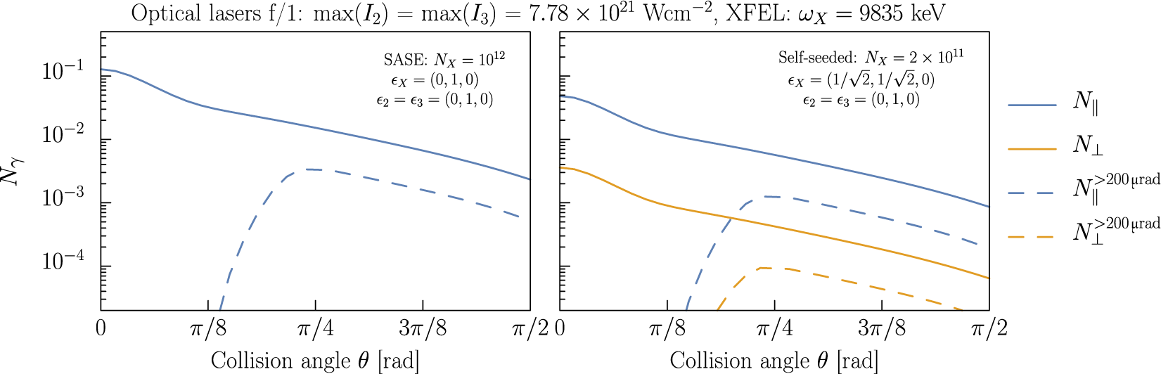
Figure 12 The number of scattered photons, parallel ( ${N}_{\parallel }$
) and perpendicular (
${N}_{\parallel }$
) and perpendicular ( ${N}_{\perp }$
) to the XFEL probe, as a function of the beam collision angle, plotted for different XFEL parameters. The probe propagates along the
${N}_{\perp }$
) to the XFEL probe, as a function of the beam collision angle, plotted for different XFEL parameters. The probe propagates along the $z$
-axis, and the collision is in the
$z$
-axis, and the collision is in the $x$
–
$x$
– $z$
plane. The dashed curves (
$z$
plane. The dashed curves ( ${N}_{\parallel, \perp}^{>200\;\unicode{x3bc} \mathrm{rad}}$
) refer to the signal falling on the detector outside a central exclusion region of radius
${N}_{\parallel, \perp}^{>200\;\unicode{x3bc} \mathrm{rad}}$
) refer to the signal falling on the detector outside a central exclusion region of radius $200\kern0.22em \unicode{x3bc} \mathrm{rad}$
. The SASE and self-seeded options are taken from Table 2. Left: example results for total scattered photons. Right: photon scattering and birefringence (polarization flip).
$200\kern0.22em \unicode{x3bc} \mathrm{rad}$
. The SASE and self-seeded options are taken from Table 2. Left: example results for total scattered photons. Right: photon scattering and birefringence (polarization flip).
To estimate the number of detectable photons, we exclude a central portion of the detector, which will be dominated by the probe XFEL photons. From knowledge of the XFEL beam and numerical simulations (such as those detailed in Section 4.2.1) we determine that a $200\kern0.22em \unicode{x3bc} \mathrm{m}$
radius for the central exclusion region on the detector would be sufficient. The entailed reduction in signal photon count is demonstrated in Figure 12. On the one hand, we would like a larger transverse momentum kick of the scattered photons so that the optical beam opening angle does not need to be made so large, and the detectable signal remains sufficient. This would suggest using lower energy XFEL photons, for example, the
$200\kern0.22em \unicode{x3bc} \mathrm{m}$
radius for the central exclusion region on the detector would be sufficient. The entailed reduction in signal photon count is demonstrated in Figure 12. On the one hand, we would like a larger transverse momentum kick of the scattered photons so that the optical beam opening angle does not need to be made so large, and the detectable signal remains sufficient. This would suggest using lower energy XFEL photons, for example, the $6\kern0.22em \mathrm{keV}$
mode. On the other hand, the cross-section,
$6\kern0.22em \mathrm{keV}$
mode. On the other hand, the cross-section, $\sigma$
, has a strong scaling with CM energy,
$\sigma$
, has a strong scaling with CM energy, ${\omega}_{\ast }$
as
${\omega}_{\ast }$
as $\sigma \propto {\omega}_{\ast}^6$
, and so to maximize the total number of photons scattered, we would use the higher energy XFEL photons, for example, the
$\sigma \propto {\omega}_{\ast}^6$
, and so to maximize the total number of photons scattered, we would use the higher energy XFEL photons, for example, the $12.9\kern0.22em \mathrm{keV}$
mode. From our analyses using the HED-HIBEF parameters, we find that the
$12.9\kern0.22em \mathrm{keV}$
mode. From our analyses using the HED-HIBEF parameters, we find that the $9.8\kern0.22em \mathrm{keV}$
mode is a good compromise in this planar three-beam scenario.
$9.8\kern0.22em \mathrm{keV}$
mode is a good compromise in this planar three-beam scenario.
Some example results are given in Table 3. Due to the bandwidth of the analyser being much narrower than the bandwidth of the XFEL beam in SASE operation, for observing birefringence we use the self-seeded parameters for which the XFEL has a narrow enough bandwidth such that scattered photons are accepted by the analyser.
Table 3 Example number of signal photons scattered in collision of the XFEL probe with two optical beams.

The planar three-beam scenario is a setup of interest for BIREF@HIBEF. As the dark-field scenario has been selected for priority access beamtime at the EuXFEL, we omit here a full discussion of the effect of optical components on the measurability of the numbers of photons detailed in Table 3, and how the HE low-energy constants ${c}_1$
and
${c}_1$
and ${c}_2$
can be determined in this setup. See Ref. [Reference Macleod and King120] for further details.
${c}_2$
can be determined in this setup. See Ref. [Reference Macleod and King120] for further details.
3.4 Other opportunities: Coulomb-assisted birefringent scattering
In the preceding sections, we have rigorously examined a variety of scenarios for detecting vacuum birefringence, each presenting unique challenges and insights. These explorations spanned across diverse experimental setups, employing a range of pump and probe fields to elucidate the nature of vacuum birefringence. These varying approaches, each with its own merits and limitations, collectively contribute to a better understanding of the phenomenon. These options are concisely summarized in Table 4. In what follows, we first provide an overview of the available choices for both pump and probe fields. Then, we venture into a new direction by combining two options for the pump field to explore a birefringent signal.
Table 4 Summary of choices for pump and probe fields in vacuum birefringence detection. Increasing the strength of the pump fields results in a smaller interaction volume, while a higher wave number in the probe fields leads to fewer photons per shot.
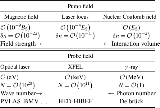
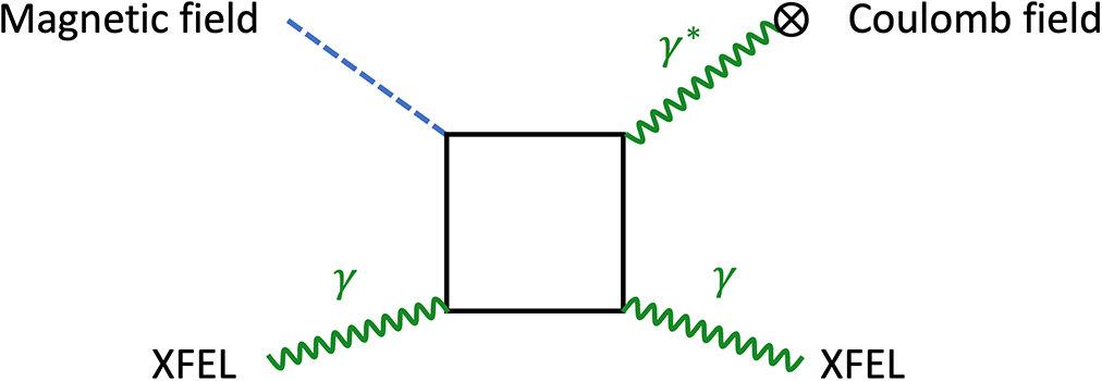
Figure 13 Feynman diagram for Coulomb-assisted birefringence.
Table 4 presents three distinct choices each for the pump and probe fields. In the case of the pump field, one can opt for a static magnetic field, laser focus or the electric field of a nucleus, each with its own set of pros and cons. For example, the first column details the characteristics of a static magnetic field, where we achieve a field strength of several teslas. This leads to an extremely small change in the vacuum refractive index ( $\delta n$
), and the other columns provide similar metrics for alternative pump field options. Regarding the probe field, there are also multiple choices. Take the optical laser, for instance: it generates a large number of photons
$\delta n$
), and the other columns provide similar metrics for alternative pump field options. Regarding the probe field, there are also multiple choices. Take the optical laser, for instance: it generates a large number of photons $N$
but with relatively low energy
$N$
but with relatively low energy $\mathcal{O}\left(\mathrm{eV}\right)$
. Table 4 illustrates various experiments that have utilized different combinations of pump and probe fields. For instance, as detailed in Section 2, experiments such as PVLAS[
Reference Ejlli, Valle, Gastaldi, Messineo, Pengo, Ruoso and Zavattini
78
] and BMV[
Reference Battesti, Da Souza, Batut, Robilliard, Bailly, Michel, Nardone, Pinard, Portugall, Trénec, Mackowski, Rikken, Vigué and Rizzo
121
] employed the options detailed in the first column: a static field as the pump and an optical laser as the probe. HED-HIBEF is designed to follow the approach outlined in the second column, using a focused array of several optical lasers for the pump field and X-rays for the probe. In addition, for the measurement of Delbrück scattering[
Reference Jarlskog, Joensson, Prünster, Schulz, Willutzki and Winter
5
, Reference Schumacher, Borchert, Smend and Rullhusen
41
], the electric field of a nucleus as pump field and high-energy gamma photons as the probe have been utilized; for more details see Ref. [Reference Ahmadiniaz, Cowan, Sauerbrey, Schramm, Schlenvoigt and Schützhold122]. In this section, we utilize the combination of a nuclear Coulomb field, denoted as
$\mathcal{O}\left(\mathrm{eV}\right)$
. Table 4 illustrates various experiments that have utilized different combinations of pump and probe fields. For instance, as detailed in Section 2, experiments such as PVLAS[
Reference Ejlli, Valle, Gastaldi, Messineo, Pengo, Ruoso and Zavattini
78
] and BMV[
Reference Battesti, Da Souza, Batut, Robilliard, Bailly, Michel, Nardone, Pinard, Portugall, Trénec, Mackowski, Rikken, Vigué and Rizzo
121
] employed the options detailed in the first column: a static field as the pump and an optical laser as the probe. HED-HIBEF is designed to follow the approach outlined in the second column, using a focused array of several optical lasers for the pump field and X-rays for the probe. In addition, for the measurement of Delbrück scattering[
Reference Jarlskog, Joensson, Prünster, Schulz, Willutzki and Winter
5
, Reference Schumacher, Borchert, Smend and Rullhusen
41
], the electric field of a nucleus as pump field and high-energy gamma photons as the probe have been utilized; for more details see Ref. [Reference Ahmadiniaz, Cowan, Sauerbrey, Schramm, Schlenvoigt and Schützhold122]. In this section, we utilize the combination of a nuclear Coulomb field, denoted as ${\mathbf{E}}^{\mathrm{ext}}$
, and the strong magnetic field
${\mathbf{E}}^{\mathrm{ext}}$
, and the strong magnetic field ${\mathbf{B}}^{\mathrm{ext}}$
provided by a focused high-intensity laser pulse as the pump field. This is coupled with an XFEL beam, which serves as the probe field; see Refs. [Reference Ahmadiniaz, Cowan, Sauerbrey, Schramm, Schlenvoigt and Schützhold122, Reference Ahmadiniaz, Bussmann, Cowan, Debus, Kluge and Schützhold123]. An illustrative Feynman diagram for this process resembles the one shown in Figure 3(a), with the key distinction being that one of the Coulomb fields is replaced by an interaction with an external magnetic field
${\mathbf{B}}^{\mathrm{ext}}$
provided by a focused high-intensity laser pulse as the pump field. This is coupled with an XFEL beam, which serves as the probe field; see Refs. [Reference Ahmadiniaz, Cowan, Sauerbrey, Schramm, Schlenvoigt and Schützhold122, Reference Ahmadiniaz, Bussmann, Cowan, Debus, Kluge and Schützhold123]. An illustrative Feynman diagram for this process resembles the one shown in Figure 3(a), with the key distinction being that one of the Coulomb fields is replaced by an interaction with an external magnetic field ${\mathbf{B}}^{\mathrm{ext}}$
; see Figure 13. This scenario may offer several advantages: the nuclear Coulomb field adds a significant momentum transfer
${\mathbf{B}}^{\mathrm{ext}}$
; see Figure 13. This scenario may offer several advantages: the nuclear Coulomb field adds a significant momentum transfer $\Delta \mathbf{k}$
to the flip of the XFEL polarization[
Reference Ahmadiniaz, Cowan, Sauerbrey, Schramm, Schlenvoigt and Schützhold
122
, Reference Ahmadiniaz, Bussmann, Cowan, Debus, Kluge and Schützhold
123
]. Compared to the past experiments measuring Delbrück scattering at photon energies
$\Delta \mathbf{k}$
to the flip of the XFEL polarization[
Reference Ahmadiniaz, Cowan, Sauerbrey, Schramm, Schlenvoigt and Schützhold
122
, Reference Ahmadiniaz, Bussmann, Cowan, Debus, Kluge and Schützhold
123
]. Compared to the past experiments measuring Delbrück scattering at photon energies $O\left(100\kern0.1em \mathrm{MeV}\right)$
[
Reference Jarlskog, Joensson, Prünster, Schulz, Willutzki and Winter
5
, Reference Akhmadaliev, Kezerashvili, Klimenko, Malyshev, Maslennikov, Milov, Milstein, Muchnoi, Naumenkov, Panin, Peleganchuk, Popov, Pospelov, Protopopov, Romanov, Shamov, Shatilov, Simonov and Tikhonov
6
, Reference Schumacher, Borchert, Smend and Rullhusen
41
], we obtain a large interaction volume whose space–time scale is set by the momentum transfer and thus exceeds the Compton wavelength. Since all involved field strengths are sub-critical, hence well below the Schwinger limit, we can use the low-field expansion of the HE Lagrangian in Equation (6) with the low-energy constants
$O\left(100\kern0.1em \mathrm{MeV}\right)$
[
Reference Jarlskog, Joensson, Prünster, Schulz, Willutzki and Winter
5
, Reference Akhmadaliev, Kezerashvili, Klimenko, Malyshev, Maslennikov, Milov, Milstein, Muchnoi, Naumenkov, Panin, Peleganchuk, Popov, Pospelov, Protopopov, Romanov, Shamov, Shatilov, Simonov and Tikhonov
6
, Reference Schumacher, Borchert, Smend and Rullhusen
41
], we obtain a large interaction volume whose space–time scale is set by the momentum transfer and thus exceeds the Compton wavelength. Since all involved field strengths are sub-critical, hence well below the Schwinger limit, we can use the low-field expansion of the HE Lagrangian in Equation (6) with the low-energy constants ${c}_1$
and
${c}_1$
and ${c}_2$
given in Equation (9). In the next step, we decompose the electric and magnetic fields in Equations (6) and (8) as
${c}_2$
given in Equation (9). In the next step, we decompose the electric and magnetic fields in Equations (6) and (8) as $\mathbf{E}\to \mathbf{E}+{\mathbf{E}}^{\mathrm{ext}}$
and
$\mathbf{E}\to \mathbf{E}+{\mathbf{E}}^{\mathrm{ext}}$
and $\mathbf{B}\to \mathbf{B}+{\mathbf{B}}^{\mathrm{ext}}$
and assume that the magnetic field
$\mathbf{B}\to \mathbf{B}+{\mathbf{B}}^{\mathrm{ext}}$
and assume that the magnetic field ${\mathbf{B}}^{\mathrm{ext}}$
is approximately constant. In addition to the static Coulomb field
${\mathbf{B}}^{\mathrm{ext}}$
is approximately constant. In addition to the static Coulomb field ${\mathbf{E}}^{\mathrm{ext}}$
of the nucleus, we have space–time-dependent XFEL fields
${\mathbf{E}}^{\mathrm{ext}}$
of the nucleus, we have space–time-dependent XFEL fields $\mathbf{E}$
and
$\mathbf{E}$
and $\mathbf{B}$
. After inserting the field decomposition into Equation (6) we obtain the effective Lagrangian for the XFEL field:
$\mathbf{B}$
. After inserting the field decomposition into Equation (6) we obtain the effective Lagrangian for the XFEL field:
 $$\begin{align}{\mathrm{\mathcal{L}}}_{\mathrm{XFEL}}=\frac{1}{2}\left(\mathbf{E}\cdot {\epsilon}^{\mathrm{ext}}\cdot \mathbf{E}+\mathbf{B}\cdot {\left({\mu}^{-1}\right)}^{\mathrm{ext}}\cdot \mathbf{B}+\mathbf{E}\cdot {\Psi}^{\mathrm{ext}}\cdot \mathbf{B}\right),\end{align}$$
where we have introduced the notation $\mathbf{E}\cdot {\epsilon}^{\mathrm{ext}}\cdot \mathbf{E}\equiv {E}_i{\epsilon}_{ij}^{\mathrm{ext}}{E}_j$
, etc., for the quadratic forms in the Lagrangian. Its Hessian defines the dynamical vacuum response functions[
Reference Baier and Breitenlohner
59
], that is, the permittivity tensor,
$\mathbf{E}\cdot {\epsilon}^{\mathrm{ext}}\cdot \mathbf{E}\equiv {E}_i{\epsilon}_{ij}^{\mathrm{ext}}{E}_j$
, etc., for the quadratic forms in the Lagrangian. Its Hessian defines the dynamical vacuum response functions[
Reference Baier and Breitenlohner
59
], that is, the permittivity tensor, ${\epsilon}_{ij}^{\mathrm{ext}}$
, the permeability tensor,
${\epsilon}_{ij}^{\mathrm{ext}}$
, the permeability tensor, ${({\mu}_{ij}^{-1})}^{\mathrm{ext}}$
, and the magneto-electric coupling tensor,
${({\mu}_{ij}^{-1})}^{\mathrm{ext}}$
, and the magneto-electric coupling tensor, ${\Psi}_{ij}^{\mathrm{ext}}$
, all of which are functions of the pump fields,
${\Psi}_{ij}^{\mathrm{ext}}$
, all of which are functions of the pump fields, ${\mathbf{E}}_{\mathrm{ext}}$
and
${\mathbf{E}}_{\mathrm{ext}}$
and ${\mathbf{B}}_{\mathrm{ext}}$
:
${\mathbf{B}}_{\mathrm{ext}}$
:
 $$\begin{align} & {\epsilon}_{ij}^{\mathrm{ext}} =\frac{2{\alpha}^2}{45{m}^4}\left(8{E}_i^{\mathrm{ext}}{E}_j^{\mathrm{ext}}+14{B}_i^{\mathrm{ext}}{B}_j^{\mathrm{ext}} +{\delta}_{ij}\left({({\mathbf{E}}^{\mathrm{ext}})}^2-{({\mathbf{B}}^{\mathrm{ext}})}^2\right)\right),\nonumber\\ & {}{\left({\mu}_{ij}^{-1}\right)}^{\mathrm{ext}}=\frac{2{\alpha}^2}{45{m}^4}\left(8{B}_i^{\mathrm{ext}}{B}_j^{\mathrm{ext}}+14{E}_i^{\mathrm{ext}}{E}_j^{\mathrm{ext}}\right.\nonumber \\&\left.\qquad\qquad +{\delta}_{ij}\left({({\mathbf{B}}^{\mathrm{ext}})}^2-{({\mathbf{E}}^{\mathrm{ext}})}^2\right)\right),\nonumber\\ & {}{\Psi}_{ij}^{\mathrm{ext}}=\frac{2{\alpha}^2}{45{m}^4}\left(-8{E}_i^{\mathrm{ext}}{B}_j^{\mathrm{ext}}+14{B}_i^{\mathrm{ext}}{E}_j^{\mathrm{ext}} +14{\delta}_{ij}({\mathbf{E}}^{\mathrm{ext}}\cdot {\mathbf{B}}^{\mathrm{ext}})\right).\end{align}$$
These tensors characterize the vacuum polarizability, which varies with the type of pump laser used, as detailed in Table 4. The equations of motion derived from Equation (40) turn into macroscopic Maxwell equations in a medium upon introducing the electric displacement field $\mathbf{D}={\epsilon}^{\mathrm{ext}}\cdot \mathbf{E}+{\Psi}^{\mathrm{ext}}\cdot \mathbf{B}$
and the magnetic displacement field
$\mathbf{D}={\epsilon}^{\mathrm{ext}}\cdot \mathbf{E}+{\Psi}^{\mathrm{ext}}\cdot \mathbf{B}$
and the magnetic displacement field $\mathbf{H}=-\left({\left({\mu}^{-1}\right)}^{\mathrm{ext}}\cdot \mathbf{B}+{\left({\Psi}^{\mathrm{ext}}\right)}^{\mathrm{T}}\cdot \mathbf{E}\right)$
. In the usual manner, a suitable combination yields the inhomogeneous wave equation:
$\mathbf{H}=-\left({\left({\mu}^{-1}\right)}^{\mathrm{ext}}\cdot \mathbf{B}+{\left({\Psi}^{\mathrm{ext}}\right)}^{\mathrm{T}}\cdot \mathbf{E}\right)$
. In the usual manner, a suitable combination yields the inhomogeneous wave equation:
 $$\begin{align}\square \mathbf{D}=\nabla \times \left[\nabla \times \mathbf{D}\right]+{\partial}_t\left[\nabla \times \mathbf{H}\right]={\mathbf{J}}^{\mathrm{eff}}.\end{align}$$
The resulting wave equation can be analysed using standard Green function methods (see e.g., Ref. [Reference Marklund and Shukla19]). The source term ${\mathbf{J}}^{\mathrm{eff}}$
, owing to its relatively small magnitude, permits the use of the Born approximation to solve the equation. To proceed we decompose the XFEL electric displacement field
${\mathbf{J}}^{\mathrm{eff}}$
, owing to its relatively small magnitude, permits the use of the Born approximation to solve the equation. To proceed we decompose the XFEL electric displacement field $\mathbf{D}$
into an incoming plane wave
$\mathbf{D}$
into an incoming plane wave ${\mathbf{D}}^{\mathrm{in}}$
and a small scattering component
${\mathbf{D}}^{\mathrm{in}}$
and a small scattering component ${\mathbf{D}}^{\mathrm{out}}$
. Assuming a stationary time-dependence of
${\mathbf{D}}^{\mathrm{out}}$
. Assuming a stationary time-dependence of ${\mathrm{e}}^{- i\omega t}$
for the XFEL, we arrive at a Helmholtz equation[
Reference Ahmadiniaz, Bussmann, Cowan, Debus, Kluge and Schützhold
123
]. This equation can be solved using Green function methods. Focusing on the long-distance behaviour, we find the following scattering amplitude[
Reference Jackson
124
]:
${\mathrm{e}}^{- i\omega t}$
for the XFEL, we arrive at a Helmholtz equation[
Reference Ahmadiniaz, Bussmann, Cowan, Debus, Kluge and Schützhold
123
]. This equation can be solved using Green function methods. Focusing on the long-distance behaviour, we find the following scattering amplitude[
Reference Jackson
124
]:
 $$\begin{align}\mathfrak{U}=\frac{1}{4\pi \mid {\mathbf{D}}_{\omega}^{\mathrm{in}}\mid}\kern0.1em {\mathbf{e}}_{\mathrm{out}}\cdot \int \mathrm{d}^3r\kern0.1em \exp \left(-i\kern0.1em {\mathbf{k}}_{\mathrm{out}}\cdot \mathbf{r}\right)\kern0.1em {\mathbf{J}}_{\omega}^{\mathrm{eff}},\end{align}$$
where ${\mathbf{k}}_{\mathrm{out}}$
is the wave vector and
${\mathbf{k}}_{\mathrm{out}}$
is the wave vector and ${\mathbf{e}}_{\mathrm{out}}$
is the polarization unit vector of the scattered XFEL radiation. The scattering amplitude straightforwardly yields the differential cross-section,
${\mathbf{e}}_{\mathrm{out}}$
is the polarization unit vector of the scattered XFEL radiation. The scattering amplitude straightforwardly yields the differential cross-section, $\mathrm{d}\sigma /\mathrm{d}\Omega ={\left|\mathfrak{U}\right|}^2$
. For Coulomb-assisted Delbrück scattering, cf. Figure 13, the amplitude can be expressed as follows:
$\mathrm{d}\sigma /\mathrm{d}\Omega ={\left|\mathfrak{U}\right|}^2$
. For Coulomb-assisted Delbrück scattering, cf. Figure 13, the amplitude can be expressed as follows:
 $$\begin{align}\mathfrak{U}&=\frac{\omega^2}{4\pi}\int \mathrm{d}^3r\kern0.1em {\mathrm{e}}^{i\Delta \mathbf{k}\cdot \mathbf{r}}\Big({\mathbf{e}}_{\mathrm{out}}\cdot {\epsilon}^{\mathrm{e}\mathrm{xt}}\cdot {\mathbf{e}}_{\mathrm{in}}+{\mathbf{e}}_{\mathrm{out}}\cdot {\Psi}^{\mathrm{e}\mathrm{xt}}\cdot \left({\mathbf{n}}_{\mathrm{in}}\times {\mathbf{e}}_{\mathrm{in}}\right) \nonumber \\&\quad +{\mathbf{e}}_{\mathrm{in}}\cdot {\Psi}^{\mathrm{e}\mathrm{xt}}\cdot \left({\mathbf{n}}_{\mathrm{out}}\times {\mathbf{e}}_{\mathrm{out}}\right)\nonumber\\ &{}\quad +\left({\mathbf{n}}_{\mathrm{out}}\times {\mathbf{e}}_{\mathrm{out}}\right)\cdot {\left({\mu}^{-1}\right)}^{\mathrm{e}\mathrm{xt}}\cdot \left({\mathbf{n}}_{\mathrm{in}}\times {\mathbf{e}}_{\mathrm{in}}\right)\Big).\end{align}$$
Here ${\mathbf{n}}_{\mathrm{in}}={\mathbf{k}}_{\mathrm{in}}/\omega$
and
${\mathbf{n}}_{\mathrm{in}}={\mathbf{k}}_{\mathrm{in}}/\omega$
and ${\mathbf{n}}_{\mathrm{out}}={\mathbf{k}}_{\mathrm{out}}/\omega$
are the initial and final propagation directions, respectively, while
${\mathbf{n}}_{\mathrm{out}}={\mathbf{k}}_{\mathrm{out}}/\omega$
are the initial and final propagation directions, respectively, while ${\mathbf{e}}_{\mathrm{in}}$
and
${\mathbf{e}}_{\mathrm{in}}$
and ${\mathbf{e}}_{\mathrm{out}}$
are the corresponding polarization vectors;
${\mathbf{e}}_{\mathrm{out}}$
are the corresponding polarization vectors; $\Delta \mathbf{k}={\mathbf{k}}_{\mathrm{in}}-{\mathbf{k}}_{\mathrm{out}}$
is the momentum transfer or recoil. Figure 13 suggests a non-vanishing contribution of the magneto-electric tensor
$\Delta \mathbf{k}={\mathbf{k}}_{\mathrm{in}}-{\mathbf{k}}_{\mathrm{out}}$
is the momentum transfer or recoil. Figure 13 suggests a non-vanishing contribution of the magneto-electric tensor ${\Psi}^{\mathrm{ext}}$
, that is, the second and the third terms of Equation (44). Since the external magnetic field
${\Psi}^{\mathrm{ext}}$
, that is, the second and the third terms of Equation (44). Since the external magnetic field ${\mathbf{B}}^{\mathrm{ext}}$
provided by an intense laser focus is approximately constant, the spatial integral in Equation (44) yields the Fourier transform of the nuclear Coulomb field,
${\mathbf{B}}^{\mathrm{ext}}$
provided by an intense laser focus is approximately constant, the spatial integral in Equation (44) yields the Fourier transform of the nuclear Coulomb field, ${\mathbf{E}}^{\mathrm{ext}}={\mathbf{e}}_{\mathrm{r}} Ze/\left(4\pi {r}^2\right)$
(
${\mathbf{E}}^{\mathrm{ext}}={\mathbf{e}}_{\mathrm{r}} Ze/\left(4\pi {r}^2\right)$
( $Z$
being the atomic number), that is,
$Z$
being the atomic number), that is, $\int \mathrm{d}^3r\kern0.1em {\mathrm{e}}^{i\Delta \mathbf{k}\cdot \mathbf{r}}{\mathbf{e}}_{\mathrm{r}} Ze/\left(4\pi {r}^2\right)= iZe\Delta \mathbf{k}/{\left|\Delta \mathbf{k}\right|}^2$
.
$\int \mathrm{d}^3r\kern0.1em {\mathrm{e}}^{i\Delta \mathbf{k}\cdot \mathbf{r}}{\mathbf{e}}_{\mathrm{r}} Ze/\left(4\pi {r}^2\right)= iZe\Delta \mathbf{k}/{\left|\Delta \mathbf{k}\right|}^2$
.
Note that the spatial integration is effectively cut off by the momentum transfer $\Delta \mathbf{k}$
, implying a large interaction volume extending over many XFEL wavelengths for small scattering angles (near-forward direction),
$\Delta \mathbf{k}$
, implying a large interaction volume extending over many XFEL wavelengths for small scattering angles (near-forward direction), $\mid {\mathbf{n}}_{\mathrm{in}}-{\mathbf{n}}_{\mathrm{out}}\mid \ll 1$
. However, when the effective interaction volume becomes of the order of the spatiotemporal scales of variation of the optical laser pulse, the approximation of a constant magnetic field can no longer be justified; see also Ref. [Reference Lee125].
$\mid {\mathbf{n}}_{\mathrm{in}}-{\mathbf{n}}_{\mathrm{out}}\mid \ll 1$
. However, when the effective interaction volume becomes of the order of the spatiotemporal scales of variation of the optical laser pulse, the approximation of a constant magnetic field can no longer be justified; see also Ref. [Reference Lee125].
Let us consider forward scattering and focus on the leading-order contribution $\sim 1/\mid \Delta \mathbf{k}\mid$
. We thus approximate
$\sim 1/\mid \Delta \mathbf{k}\mid$
. We thus approximate ${\mathbf{n}}_{\mathrm{in}}\approx {\mathbf{n}}_{\mathrm{out}}\equiv \mathbf{n}$
and consider the birefringent signal where
${\mathbf{n}}_{\mathrm{in}}\approx {\mathbf{n}}_{\mathrm{out}}\equiv \mathbf{n}$
and consider the birefringent signal where ${\mathbf{e}}_{\mathrm{in}}$
and
${\mathbf{e}}_{\mathrm{in}}$
and $\mathbf{n}$
are (nearly) orthogonal, that is,
$\mathbf{n}$
are (nearly) orthogonal, that is, ${\mathbf{e}}_{\mathrm{in}}\approx \mp \mathbf{n}\times {\mathbf{e}}_{\mathrm{out}}$
and
${\mathbf{e}}_{\mathrm{in}}\approx \mp \mathbf{n}\times {\mathbf{e}}_{\mathrm{out}}$
and ${\mathbf{e}}_{\mathrm{out}}\approx \pm \mathbf{n}\times {\mathbf{e}}_{\mathrm{in}}$
. (The
${\mathbf{e}}_{\mathrm{out}}\approx \pm \mathbf{n}\times {\mathbf{e}}_{\mathrm{in}}$
. (The $\mp$
and
$\mp$
and $\pm$
symbols refer to two possible orientations of
$\pm$
symbols refer to two possible orientations of ${\mathbf{e}}_{\mathrm{in}}$
and
${\mathbf{e}}_{\mathrm{in}}$
and ${\mathbf{e}}_{\mathrm{out}}$
: either parallel or anti-parallel to the cross-product of
${\mathbf{e}}_{\mathrm{out}}$
: either parallel or anti-parallel to the cross-product of $\mathbf{n}$
with the other polarization vector.) This simplifies the integrand in Equation (44), and the birefringent amplitude is finally given by the following:
$\mathbf{n}$
with the other polarization vector.) This simplifies the integrand in Equation (44), and the birefringent amplitude is finally given by the following:
 $$\begin{align}{\mathfrak{U}}_{\perp}^{\Psi^{\mathrm{ext}}} &=\pm i\kern0.1em \frac{12{\alpha}^2}{45{m}^4}\kern0.1em \frac{Ze}{{\left(\Delta \mathbf{k}\right)}^2}\frac{\omega^2}{4\pi}\left(\left({\mathbf{e}}_{\mathrm{out}}\cdot {\mathbf{B}}^{\mathrm{ext}}\right)\left({\mathbf{e}}_{\mathrm{out}}\cdot \Delta \mathbf{k}\right) \right. \nonumber \\&\left. \quad -\left({\mathbf{e}}_{\mathrm{in}}\cdot {\mathbf{B}}^{\mathrm{ext}}\right)\left({\mathbf{e}}_{\mathrm{in}}\cdot \Delta \mathbf{k}\right)\right).\end{align}$$
We maximize the birefringence signal by aligning $\Delta \mathbf{k}$
with
$\Delta \mathbf{k}$
with ${\mathbf{B}}^{\mathrm{ext}}$
and
${\mathbf{B}}^{\mathrm{ext}}$
and ${\mathbf{e}}_{\mathrm{in}}$
(or
${\mathbf{e}}_{\mathrm{in}}$
(or ${\mathbf{e}}_{\mathrm{out}}$
). Assuming a strong magnetic field of the order of
${\mathbf{e}}_{\mathrm{out}}$
). Assuming a strong magnetic field of the order of ${B}^{\mathrm{ext}}={10}^6\;\mathrm{T}$
(which can be achieved through laser focusing) and a large XFEL frequency of
${B}^{\mathrm{ext}}={10}^6\;\mathrm{T}$
(which can be achieved through laser focusing) and a large XFEL frequency of $\omega =24\;\mathrm{keV}$
(which involves additional experimental challenges), the birefringence signal is encoded in the differential cross-section in the forward direction:
$\omega =24\;\mathrm{keV}$
(which involves additional experimental challenges), the birefringence signal is encoded in the differential cross-section in the forward direction:
 $$\begin{align}\frac{\mathrm{d}{\sigma}_{\perp}^{\Psi^{\mathrm{ext}}}}{\mathrm{d}\Omega}={\left|{\mathfrak{U}}_{\perp}^{\Psi^{\mathrm{ext}}}\right|}^2\approx {10}^{-25}\frac{Z^2}{{\left(\Delta \mathbf{k}\right)}^2}. \end{align}$$
The magnitude of the signal in Equation (46) is comparable to the other proposals for the vacuum birefringence experiments discussed above. In the Coulomb-assisted scenario, there are two main enhancement factors: firstly, the large number, $\mathcal{O}\left({10}^{12}\right)$
, of polarized XFEL photons; secondly, the large number
$\mathcal{O}\left({10}^{12}\right)$
, of polarized XFEL photons; secondly, the large number $N$
of nuclei. In one possible scenario, a cubic carbon cluster with an edge length of
$N$
of nuclei. In one possible scenario, a cubic carbon cluster with an edge length of $100\kern0.1em \mathrm{nm}$
is ionized completely using the pre-pulse of a high-intensity laser of the order of
$100\kern0.1em \mathrm{nm}$
is ionized completely using the pre-pulse of a high-intensity laser of the order of $\mathcal{O}\left({10}^{22}\kern0.22em \mathrm{W}/{\mathrm{cm}}^2\right)$
. For small momentum transfer (of the order of eV), particle-in-cell (PIC) simulations show that the amplitudes of
$\mathcal{O}\left({10}^{22}\kern0.22em \mathrm{W}/{\mathrm{cm}}^2\right)$
. For small momentum transfer (of the order of eV), particle-in-cell (PIC) simulations show that the amplitudes of $N={10}^8$
nuclei would have the same phase and add up coherently, thus acting as one giant nucleus of charge
$N={10}^8$
nuclei would have the same phase and add up coherently, thus acting as one giant nucleus of charge ${Z}_{\mathrm{eff}}= NZ$
. The birefringent signal would be of the order of
${Z}_{\mathrm{eff}}= NZ$
. The birefringent signal would be of the order of $\mathcal{O}\left({10}^{-5}\right)$
photons per shot and thus could be detected in complete analogy with the scenarios discussed above; see also Refs. [Reference Inada, Yamazaki, Yamaji, Seino, Fan, Kamioka, Namba and Asai44, Reference Yamaji, Inada, Yamazaki, Namba, Asai, Kobayashi, Tamasaku, Tanaka, Inubushi, Sawada, Yabashi and Ishikawa45, Reference Heinzl, Liesfeld, Amthor, Schwoerer, Sauerbrey and Wipf67, Reference Battesti, Beard, Böser, Bruyant, Budker, Crooker, Daw, Flambaum, Inada, Irastorza, Karbstein, Kim, Kozlov, Melhem, Phipps, Pugnat, Rikken, Rizzo, Schott, Semertzidis and Zavattini79, Reference Schlenvoigt, Heinzl, Schramm, Cowan and Sauerbrey84]. For a more detailed discussion, we refer to the recent publications in Refs. [Reference Ahmadiniaz, Bussmann, Cowan, Debus, Kluge and Schützhold123, Reference Ahmadiniaz, Cowan, Ding, Lopez, Sauerbrey, Shaisultanov and Schützhold126], which also address a number of potential background processes, including nuclear Thomson scattering, nuclear resonances, Delbrück scattering and electronic Compton scattering. Among these processes, electronic Compton scattering seems the most important.
$\mathcal{O}\left({10}^{-5}\right)$
photons per shot and thus could be detected in complete analogy with the scenarios discussed above; see also Refs. [Reference Inada, Yamazaki, Yamaji, Seino, Fan, Kamioka, Namba and Asai44, Reference Yamaji, Inada, Yamazaki, Namba, Asai, Kobayashi, Tamasaku, Tanaka, Inubushi, Sawada, Yabashi and Ishikawa45, Reference Heinzl, Liesfeld, Amthor, Schwoerer, Sauerbrey and Wipf67, Reference Battesti, Beard, Böser, Bruyant, Budker, Crooker, Daw, Flambaum, Inada, Irastorza, Karbstein, Kim, Kozlov, Melhem, Phipps, Pugnat, Rikken, Rizzo, Schott, Semertzidis and Zavattini79, Reference Schlenvoigt, Heinzl, Schramm, Cowan and Sauerbrey84]. For a more detailed discussion, we refer to the recent publications in Refs. [Reference Ahmadiniaz, Bussmann, Cowan, Debus, Kluge and Schützhold123, Reference Ahmadiniaz, Cowan, Ding, Lopez, Sauerbrey, Shaisultanov and Schützhold126], which also address a number of potential background processes, including nuclear Thomson scattering, nuclear resonances, Delbrück scattering and electronic Compton scattering. Among these processes, electronic Compton scattering seems the most important.
Another background atomic effect that could flip the polarization of X-ray photons is birefringence and dichroism of atomic X-ray susceptibility due to the alignment of electrons in ions generated by strong-field ionization by the polarized optical laser pulse. The X-ray dichroism of ionized krypton gas was experimentally demonstrated in Refs. [Reference Young, Arms, Dufresne, Dunford, Ederer, Höhr, Kanter, Krässig, Landahl, Peterson, Rudati, Santra and Southworth127–Reference Goulielmakis, Loh, Wirth, Santra, Rohringer, Yakovlev, Zherebtsov, Pfeifer, Azzeer, Kling, Leone and Krausz129] and theoretically studied in Refs. [Reference Santra, Dunford and Young130,Reference Rohringer and Santra131] for X-rays resonant to transition between the 1s core atomic orbital and 4p3/2 valence atomic orbital where an aligned electron hole was produced. From these studies, the probability of polarization flipping can be estimated as $\sim {\left(\sin \left(2\theta \right)n{\lambda}^2L\Delta {\rho}_{\mathrm{aniso}}\right)}^2{A}^2/\left(\Delta {\omega}^2+{\gamma}^2/4\right)$
, where
$\sim {\left(\sin \left(2\theta \right)n{\lambda}^2L\Delta {\rho}_{\mathrm{aniso}}\right)}^2{A}^2/\left(\Delta {\omega}^2+{\gamma}^2/4\right)$
, where $\theta$
is an angle between the polarizations of the optical and X-ray pulses;
$\theta$
is an angle between the polarizations of the optical and X-ray pulses; $n$
and
$n$
and $L$
are the concentration and the length of the gas sample, respectively;
$L$
are the concentration and the length of the gas sample, respectively; $\lambda$
is the X-ray wavelength;
$\lambda$
is the X-ray wavelength; $\Delta {\rho}_{\mathrm{aniso}}$
is the difference between probabilities of finding a valence orbital hole with distinct projection quantum numbers – this quantity describes the alignment of the valence hole;
$\Delta {\rho}_{\mathrm{aniso}}$
is the difference between probabilities of finding a valence orbital hole with distinct projection quantum numbers – this quantity describes the alignment of the valence hole; $A$
,
$A$
, $\Delta \omega$
and
$\Delta \omega$
and $\gamma$
are the spontaneous emission rate, the detuning and the linewidth, respectively, for the corresponding valence-to-core transition. For the case of strong-field ionized
$\gamma$
are the spontaneous emission rate, the detuning and the linewidth, respectively, for the corresponding valence-to-core transition. For the case of strong-field ionized ${\mathrm{Kr}}^{+}4{\mathrm{p}}^{-1}$
, the alignment of the valence hole
${\mathrm{Kr}}^{+}4{\mathrm{p}}^{-1}$
, the alignment of the valence hole $\Delta {\rho}_{\mathrm{aniso}}$
can reach the value of
$\Delta {\rho}_{\mathrm{aniso}}$
can reach the value of $64\%$
, and for an atomic concentration 10
$64\%$
, and for an atomic concentration 10 ${}^{18}\kern0.1em {\mathrm{cm}}^{-3}$
, an interaction length of a few mm and an X-ray photon energy resonant to the valence-to-core transition, the polarization flipping probability could reach
${}^{18}\kern0.1em {\mathrm{cm}}^{-3}$
, an interaction length of a few mm and an X-ray photon energy resonant to the valence-to-core transition, the polarization flipping probability could reach $\mathcal{O}$
(10
$\mathcal{O}$
(10 ${}^{-5}$
). With decreasing gas concentration and increasing detuning, this probability rapidly drops off; thus avoiding the valence-to-core transition is necessary to suppress the atomic birefringence background. From the atomic, molecular and optical (AMO) and plasma physics point of view, the high-purity X-ray polarimetry measurements described in this letter could provide unique insights into the anisotropy properties of atomic transitions.
${}^{-5}$
). With decreasing gas concentration and increasing detuning, this probability rapidly drops off; thus avoiding the valence-to-core transition is necessary to suppress the atomic birefringence background. From the atomic, molecular and optical (AMO) and plasma physics point of view, the high-purity X-ray polarimetry measurements described in this letter could provide unique insights into the anisotropy properties of atomic transitions.
4 Plans for experimental implementation
Based on the expected signal and noise estimates presented in this paper, as well as on the experimental feasibility, the dark-field approach was selected to be pursued via the HIBEF user consortium priority access at the EuXFEL. The first X-ray-only beamtime was allocated for March 2024. It was devoted to carrying out a proof-of-principle experiment of the dark-field concept at the XFEL. The outcomes of this campaign are currently being analysed and will determine the setup to be implemented for the actual discovery experiment.
4.1 Conventional scenario
The decisive bottlenecks in the conventional scenario are the quality of the X-ray polarizers and the X-ray lenses. For the former, early works suggested that an extinction ratio of the order of ${10}^{-10}$
would be necessary to prove vacuum birefringence induced by a petawatt-class laser. The extinction ratio is also known as polarization purity. More detailed analyses, together with the fact that only
${10}^{-10}$
would be necessary to prove vacuum birefringence induced by a petawatt-class laser. The extinction ratio is also known as polarization purity. More detailed analyses, together with the fact that only $300\kern0.22em \mathrm{TW}$
is available at the EuXFEL, led to the insight that an extinction ratio of
$300\kern0.22em \mathrm{TW}$
is available at the EuXFEL, led to the insight that an extinction ratio of ${10}^{-12}$
is actually required for the X-ray polarimeter. Of equal importance is that the X-ray lenses do not compromise the polarization purity.
${10}^{-12}$
is actually required for the X-ray polarimeter. Of equal importance is that the X-ray lenses do not compromise the polarization purity.
At the University of Jena and the Helmholtz Institute Jena, a research and development programme to eliminate these two bottlenecks was started about 15 years ago. The polarizers are perfect crystals into which a trench is cut – which is why they are referred to as channel-cut crystals or simply channel cuts (CCs). The wavelength is chosen such that the X-rays are Bragg-reflected at the (inner) walls of the channel at a Bragg angle of 45°, the Brewster angle for X-rays. At the Brewster angle, the polarization component parallel to the diffraction plane (p-component) of the X-rays field is suppressed. Zig-zagging multiple successive reflections increases the suppression of the p-component. For some crystals attractive for X-ray polarimetry – namely diamond – cutting a channel is not an option. In this case, one would precision-mount two separate crystals perfectly in parallel, an arrangement known as artificial or QCC.

Figure 14 High-precision X-ray polarimetry. Left: the polarimeter consists of two channel-cut crystals acting as polarizer and analyser, respectively. Not shown is the telescope in between both and the optical laser responsible for polarizing the vacuum. Right: extinction curve around ${0.01}^{\circ }$
of the crossed-polarizer position reproduced from Ref. [Reference Schulze, Grabiger, Loetzsch, Marx-Glowna, Schmitt, Garcia, Hippler, Huang, Karbstein, Konôpková, Schlenvoigt, Schwinkendorf, Strohm, Toncian, Uschmann, Wille, Zastrau, Röhlsberger, Stöhlker, Cowan and Paulus72]. At a few data points, the corresponding detector signal is displayed: in the crossed-polarizer position not a single photon reaches the detector. To the level tested in this experiment, the polarizers are perfect.
${0.01}^{\circ }$
of the crossed-polarizer position reproduced from Ref. [Reference Schulze, Grabiger, Loetzsch, Marx-Glowna, Schmitt, Garcia, Hippler, Huang, Karbstein, Konôpková, Schlenvoigt, Schwinkendorf, Strohm, Toncian, Uschmann, Wille, Zastrau, Röhlsberger, Stöhlker, Cowan and Paulus72]. At a few data points, the corresponding detector signal is displayed: in the crossed-polarizer position not a single photon reaches the detector. To the level tested in this experiment, the polarizers are perfect.
As early as 2010, an extinction ratio of $1.5\times {10}^{-9}$
at
$1.5\times {10}^{-9}$
at $6.457\kern0.22em \mathrm{keV}$
photon energy and of
$6.457\kern0.22em \mathrm{keV}$
photon energy and of $9.0\times {10}^{-9}$
at
$9.0\times {10}^{-9}$
at $12.914\kern0.22em \mathrm{keV}$
was demonstrated. The (400) and (800) Bragg reflexes of Si were used[
Reference Marx, Uschmann, Höfer, Lötzsch, Wehrhan, Förster, Kaluza, Stöhlker, Gies, Detlefs, Roth, Härtwig and Paulus
132
]. Advances in the production and processing of the crystals and improvements in the brilliance of X-ray sources led relatively quickly to a further improvement in polarization purity to
$12.914\kern0.22em \mathrm{keV}$
was demonstrated. The (400) and (800) Bragg reflexes of Si were used[
Reference Marx, Uschmann, Höfer, Lötzsch, Wehrhan, Förster, Kaluza, Stöhlker, Gies, Detlefs, Roth, Härtwig and Paulus
132
]. Advances in the production and processing of the crystals and improvements in the brilliance of X-ray sources led relatively quickly to a further improvement in polarization purity to $2.4\times {10}^{-10}$
and
$2.4\times {10}^{-10}$
and $5.7\times {10}^{-10}$
for the same X-ray wavelengths as above[
Reference Marx, Schulze, Uschmann, Kämpfer, Lötzsch, Wehrhan, Wagner, Detlefs, Roth, Härtwig, Förster, Stöhlker and Paulus
85
]. The originally communicated requirements on X-ray polarimetry to detect vacuum birefringence were thus largely fulfilled. While these requirements were to become more and more demanding, some of the opportunities arising from the advent of polarizers providing polarization purities several orders of magnitude better than the previous state-of-the-art were quickly exploited (e.g., Refs. [Reference Marx-Glowna, Grabiger, Lötzsch, Uschmann, Schmitt, Schulze, Last, Roth, Antipov, Schlenvoigt, Sergueev, Leupold, Röhlsberger and Paulus21, Reference Marx, Schulze, Uschmann, Kämpfer, Lötzsch, Wehrhan, Wagner, Detlefs, Roth, Härtwig, Förster, Stöhlker and Paulus85, Reference Schulze, Loetzsch, Rüffer, Uschmann, Röhlsberger and Paulus133, Reference Schmitt, Joly, Schulze, Marx-Glowna, Uschmann, Grabiger, Bernhardt, Loetzsch, Juhin, Debray, Wille, Yavaş, Paulus and Röhlsberger134]). Prominent applications were the detection of quantum optics and QED effects in the X-ray range[
Reference Heeg, Wille, Schlage, Guryeva, Schumacher, Uschmann, Schulze, Marx, Kämpfer, Paulus, Röhlsberger and Evers
135
–
Reference Haber, Schulze, Schlage, Loetzsch, Bocklage, Gurieva, Bernhardt, Wille, Rüffer, Uschmann, Paulus and Röhlsberger
137
].
$5.7\times {10}^{-10}$
for the same X-ray wavelengths as above[
Reference Marx, Schulze, Uschmann, Kämpfer, Lötzsch, Wehrhan, Wagner, Detlefs, Roth, Härtwig, Förster, Stöhlker and Paulus
85
]. The originally communicated requirements on X-ray polarimetry to detect vacuum birefringence were thus largely fulfilled. While these requirements were to become more and more demanding, some of the opportunities arising from the advent of polarizers providing polarization purities several orders of magnitude better than the previous state-of-the-art were quickly exploited (e.g., Refs. [Reference Marx-Glowna, Grabiger, Lötzsch, Uschmann, Schmitt, Schulze, Last, Roth, Antipov, Schlenvoigt, Sergueev, Leupold, Röhlsberger and Paulus21, Reference Marx, Schulze, Uschmann, Kämpfer, Lötzsch, Wehrhan, Wagner, Detlefs, Roth, Härtwig, Förster, Stöhlker and Paulus85, Reference Schulze, Loetzsch, Rüffer, Uschmann, Röhlsberger and Paulus133, Reference Schmitt, Joly, Schulze, Marx-Glowna, Uschmann, Grabiger, Bernhardt, Loetzsch, Juhin, Debray, Wille, Yavaş, Paulus and Röhlsberger134]). Prominent applications were the detection of quantum optics and QED effects in the X-ray range[
Reference Heeg, Wille, Schlage, Guryeva, Schumacher, Uschmann, Schulze, Marx, Kämpfer, Paulus, Röhlsberger and Evers
135
–
Reference Haber, Schulze, Schlage, Loetzsch, Bocklage, Gurieva, Bernhardt, Wille, Rüffer, Uschmann, Paulus and Röhlsberger
137
].
In order to achieve further improvements in polarization purity, the limiting factors had to be identified[ Reference Schulze 138 , Reference Marx-Glowna, Schulze, Uschmann, Kämpfer, Weber, Hahn, Wille, Schlage, Röhlsberger, Förster, Stöhlker and Paulus 139 ] and eliminated. These are the so-called Umweganregungen and the finite divergence of the X-rays. Strictly speaking, the latter is not a real problem, as it only occurs at the synchrotron and laboratory sources used for polarimeter development, whereas the divergence of the XFEL beam is negligible. With regard to the Umweganregungen, it turned out that these cannot be avoided in principle. However, there are certain highly symmetrical reflexes for which all of them interfere destructively. What is required, though, is a highly precise adjustment not only of the Bragg angle, but also of the azimuthal orientation of the polarimeter crystals, which is the degree of freedom that can be exploited by a rotation around the normal of the diffracting lattice planes. Novel methods have been developed for this task that enable quick adjustment of the polarimeter crystals and thus efficient use of the precious XFEL beamtime.
In parallel, another branch of the research and development of X-ray polarimeters was the use of diamond crystals. These are advantageous for several reasons. Notable among these are the small lattice constant, which allows the use of shorter wavelengths, the low atomic number, which is advantageous with regard to Umweganregungen, the high reflectivity of almost 100% and, finally, the excellent thermal conductivity. First experiments were performed with relatively cheap CVD crystals in a QCC setup with only two reflections[
Reference Bernhardt, Marx-Glowna, Schulze, Grabiger, Haber, Detlefs, Loetzsch, Kämpfer, Röhlsberger, Förster, Stöhlker, Uschmann and Paulus
140
]. Nevertheless, a polarization purity of $8.9\times {10}^{-10}$
at
$8.9\times {10}^{-10}$
at $9.837\kern0.22em \mathrm{keV}$
((400) Bragg reflection) was obtained, limited by the divergence of the synchrotron radiation. With four crystals for both the polarizer and the analyser, and some control on the beam divergence, another record polarization purity of
$9.837\kern0.22em \mathrm{keV}$
((400) Bragg reflection) was obtained, limited by the divergence of the synchrotron radiation. With four crystals for both the polarizer and the analyser, and some control on the beam divergence, another record polarization purity of $1.4\times {10}^{-10}$
was achieved[
Reference Bernhardt, Schmitt, Grabiger, Marx-Glowna, Loetzsch, Wille, Bessas, Chumakov, Rüffer, Röhlsberger, Stöhlker, Uschmann, Paulus and Schulze
141
].
$1.4\times {10}^{-10}$
was achieved[
Reference Bernhardt, Schmitt, Grabiger, Marx-Glowna, Loetzsch, Wille, Bessas, Chumakov, Rüffer, Röhlsberger, Stöhlker, Uschmann, Paulus and Schulze
141
].
The first experiment at a free-electron X-ray laser was performed at the HED instrument of the EuXFEL. The silicon 400 reflection and six reflections in the CC were used. A polarization purity of $8\times {10}^{-11}$
was achieved; see Figure 14 for an illustration. It should be emphasized that this number is not determined by the quality of the polarizers but rather by the photon flux of the XFEL. In other words,
$8\times {10}^{-11}$
was achieved; see Figure 14 for an illustration. It should be emphasized that this number is not determined by the quality of the polarizers but rather by the photon flux of the XFEL. In other words, $8\times {10}^{-11}$
is the upper limit for the actual extinction ratio; the extinction curve is in fact compatible with perfect polarization[
Reference Schulze, Grabiger, Loetzsch, Marx-Glowna, Schmitt, Garcia, Hippler, Huang, Karbstein, Konôpková, Schlenvoigt, Schwinkendorf, Strohm, Toncian, Uschmann, Wille, Zastrau, Röhlsberger, Stöhlker, Cowan and Paulus
72
]. It should also be emphasized that the limited photon flux was due to limited beamtime, the XFEL running in SASE mode and other factors, that is, they do not constitute principal road blocks. This is highlighted by the fact that the present record polarization purity of
$8\times {10}^{-11}$
is the upper limit for the actual extinction ratio; the extinction curve is in fact compatible with perfect polarization[
Reference Schulze, Grabiger, Loetzsch, Marx-Glowna, Schmitt, Garcia, Hippler, Huang, Karbstein, Konôpková, Schlenvoigt, Schwinkendorf, Strohm, Toncian, Uschmann, Wille, Zastrau, Röhlsberger, Stöhlker, Cowan and Paulus
72
]. It should also be emphasized that the limited photon flux was due to limited beamtime, the XFEL running in SASE mode and other factors, that is, they do not constitute principal road blocks. This is highlighted by the fact that the present record polarization purity of $\left(1.4\pm 0.9\right)\times {10}^{-11}$
was achieved at a third generation synchrotron facility[
Reference Marx-Glowna, Grabiger, Lötzsch, Uschmann, Schmitt, Schulze, Last, Roth, Antipov, Schlenvoigt, Sergueev, Leupold, Röhlsberger and Paulus
21
]. The theoretical limit for the polarization purity as determined by the finite laser beam divergence is of the order of
$\left(1.4\pm 0.9\right)\times {10}^{-11}$
was achieved at a third generation synchrotron facility[
Reference Marx-Glowna, Grabiger, Lötzsch, Uschmann, Schmitt, Schulze, Last, Roth, Antipov, Schlenvoigt, Sergueev, Leupold, Röhlsberger and Paulus
21
]. The theoretical limit for the polarization purity as determined by the finite laser beam divergence is of the order of ${10}^{-14}$
. It has yet to be shown whether this limit can be reached or whether other effects kick in.
${10}^{-14}$
. It has yet to be shown whether this limit can be reached or whether other effects kick in.
Another bottleneck is the lenses of the X-ray telescope. Due to a refractive index slightly smaller than unity in the X-ray regime, stacks of concave lenses must be used, so-called compound refractive lenses (CRLs). Irrespective of that, it is known that X-ray diffraction in crystals can lead to birefringence. It is also known that metals, including beryllium, the preferred material for X-ray lenses, have a micro-crystalline structure. Accordingly, the question has been whether this is indeed a limiting factor and, if so, how to bypass it. The Jena group has addressed both. In short, the answer is that there is little if any hope that beryllium, which is attractive because of high transmission, can be used. Already $500\kern0.22em \unicode{x3bc} \mathrm{m}$
of beryllium degrades the polarization purity to the level of
$500\kern0.22em \unicode{x3bc} \mathrm{m}$
of beryllium degrades the polarization purity to the level of ${10}^{-6}$
[
Reference Grabiger, Marx-Glowna, Uschmann, Loetzsch, Paulus and Schulze
142
].
${10}^{-6}$
[
Reference Grabiger, Marx-Glowna, Uschmann, Loetzsch, Paulus and Schulze
142
].
One alternative is the use of amorphous lens materials. Two options have been tested so far: CRLs made from glassy carbon and lithographically produced CRLs made from the photoresist SU-8. The disadvantage of the latter is that the production method only allows one-dimensional focusing. Therefore, two SU-8 CRLs, rotated by 90° with respect to each other, have to be used for focusing and recollimation. This reduces the transmission of the total setup. On the other hand, these lenses are of very good optical quality and allow close to diffraction-limited performance[ Reference Grabiger, Marx-Glowna, Uschmann, Loetzsch, Paulus and Schulze 142 ]. For glassy carbon, the situation was exactly the opposite. Meanwhile, better components have become available and tests will be carried out soon.

Figure 15 Experimental setup for the dark-field proof-of-principle experiment at the HED instrument of the EuXFEL. For completeness, here also the ReLaX beam path for the counter-propagating geometry is indicated.
Still another alternative, at first glance maybe paradoxically, is lenses made from perfect crystals, specifically diamond. They can be rotated around the optical axis such that they exhibit no birefringence. Also this option will be tested soon.
The conclusion is that the conventional scenario is still very promising and could indeed be the fastest way to prove vacuum birefringence. Essentially, it must be shown that the polarimeters can achieve an extinction ratio of the order of ${10}^{-12}$
. So far, there is no evidence whatsoever that this might not be the case.
${10}^{-12}$
. So far, there is no evidence whatsoever that this might not be the case.
4.2 Dark-field scenario
The setup described in Section 3.2 and schematically shown in Figure 9 was adapted to fit the experimental conditions of the HED instrument of the EuXFEL for the proof-of-principle experiment, as can be seen in Figure 15. The experiment is designed to be used with XFEL photon energy of $8766\kern0.22em \mathrm{eV}$
, so that a 440 plane of a germanium crystal can be used as a polarization analyser. The XFEL beam is coming from the left-hand side of the picture, entering the IC1 experimental chamber about
$8766\kern0.22em \mathrm{eV}$
, so that a 440 plane of a germanium crystal can be used as a polarization analyser. The XFEL beam is coming from the left-hand side of the picture, entering the IC1 experimental chamber about $-1.2\kern0.22em \mathrm{m}$
upstream from the interaction point. The whole setup is in vacuum chambers up until the Kapton window located before the detectors, at about
$-1.2\kern0.22em \mathrm{m}$
upstream from the interaction point. The whole setup is in vacuum chambers up until the Kapton window located before the detectors, at about $5\kern0.1em \mathrm{m}$
downstream from the target chamber center (TCC). At the entrance point (
$5\kern0.1em \mathrm{m}$
downstream from the target chamber center (TCC). At the entrance point ( $-1.1\kern0.22em \mathrm{m}$
), obstacle O1 is located, which is made of a vertical wire-like structure with a diameter of 125–150
$-1.1\kern0.22em \mathrm{m}$
), obstacle O1 is located, which is made of a vertical wire-like structure with a diameter of 125–150 $\unicode{x3bc} \mathrm{m}$
to block the central part of the beam. The focusing lens (L1) is located 47 cm upstream from focus, and consists of 12 beryllium lenses with a
$\unicode{x3bc} \mathrm{m}$
to block the central part of the beam. The focusing lens (L1) is located 47 cm upstream from focus, and consists of 12 beryllium lenses with a $50\kern0.22em \unicode{x3bc} \mathrm{m}$
central radius of curvature. The beryllium lenses have a
$50\kern0.22em \unicode{x3bc} \mathrm{m}$
central radius of curvature. The beryllium lenses have a $400\kern0.22em \unicode{x3bc} \mathrm{m}$
diameter, which is the limiting factor for the incoming beam size. Just after the lens stack, obstacle O2 is located, made of simple wire with a size matching O1. A pinhole of about
$400\kern0.22em \unicode{x3bc} \mathrm{m}$
diameter, which is the limiting factor for the incoming beam size. Just after the lens stack, obstacle O2 is located, made of simple wire with a size matching O1. A pinhole of about $50\kern0.22em \unicode{x3bc} \mathrm{m}$
diameter is placed exactly in the focus, which prevents radiation scattered on the first lens from propagating further. The image of O1 projected by lens L1 is at the position 85 cm downstream from the focus, where aperture A1 is located. The scattering on the edges of these slits is a critical factor for the success of the setup, and therefore several possibilities for how to limit the beam are being pursued, as described further. The second lens stack (L2), consisting of six lenses of the same type as lens 1, is located 114 cm downstream from focus, to image the focal plane onto the detector plane. An intermediate aperture (A2) is located in a separate chamber at the image of obstacle O2, that is, about
$50\kern0.22em \unicode{x3bc} \mathrm{m}$
diameter is placed exactly in the focus, which prevents radiation scattered on the first lens from propagating further. The image of O1 projected by lens L1 is at the position 85 cm downstream from the focus, where aperture A1 is located. The scattering on the edges of these slits is a critical factor for the success of the setup, and therefore several possibilities for how to limit the beam are being pursued, as described further. The second lens stack (L2), consisting of six lenses of the same type as lens 1, is located 114 cm downstream from focus, to image the focal plane onto the detector plane. An intermediate aperture (A2) is located in a separate chamber at the image of obstacle O2, that is, about $4\kern0.22em \mathrm{m}$
downstream of focus. Six to seven metres downstream, at the end of the experimental hutch, is where the detector bench is located. This can either host detectors in the direct beam, which is useful for initial alignment and testing, or can be used for measurement of the polarization distinction. Alternatively, an analyser setup hosting two detectors and Ge crystal can be put in the hutch, as described below.
$4\kern0.22em \mathrm{m}$
downstream of focus. Six to seven metres downstream, at the end of the experimental hutch, is where the detector bench is located. This can either host detectors in the direct beam, which is useful for initial alignment and testing, or can be used for measurement of the polarization distinction. Alternatively, an analyser setup hosting two detectors and Ge crystal can be put in the hutch, as described below.
In order to align and monitor the X-ray beam, the diode screen with the photodiode, as well as several fluorescent screens, is located along the beam propagation axis. For the ultimate discovery experiment the ReLaX optical beam will counter-propagate with the XFEL beam, focused down by an $f/1$
off-axis parabolic mirror (OAP). In this experiment the ReLaX beam is expected to deliver 300 TW in 25 fs, and be focused down to a focal spot FWHM diameter of
$f/1$
off-axis parabolic mirror (OAP). In this experiment the ReLaX beam is expected to deliver 300 TW in 25 fs, and be focused down to a focal spot FWHM diameter of $1.3\kern0.22em \unicode{x3bc} \mathrm{m}$
. This focusing scheme, beam routing and corresponding diagnostics are yet to be developed.
$1.3\kern0.22em \unicode{x3bc} \mathrm{m}$
. This focusing scheme, beam routing and corresponding diagnostics are yet to be developed.

Figure 16 Result of the diffractive simulation. The sub-figures show the 2D intensity profiles of the beam along the beam path at various positions: (a) just behind the first obstacle, (b) at the pinhole position, close to beam focus, (c) before aperture A1, (d) behind aperture A1, (e) at an intermediate position and (f) at the detector, with a red square indicating the area into which the signal scattered at focus would be imaged. The axes are in units of $\unicode{x3bc}$
m and the colour scale is logarithmic over three orders of magnitude.
$\unicode{x3bc}$
m and the colour scale is logarithmic over three orders of magnitude.
There are two key parameters to evaluate the quality of the dark-field setup. The shadow factor $\mathcal{S}$
was already defined in the theory in Section 3.2. The definition from the experimental point of view is that it is the ratio of X-ray photons in the active area of the final detector to the number of X-ray photons entering the chamber if there is no scattering at the focal spot involved.
$\mathcal{S}$
was already defined in the theory in Section 3.2. The definition from the experimental point of view is that it is the ratio of X-ray photons in the active area of the final detector to the number of X-ray photons entering the chamber if there is no scattering at the focal spot involved.
The aim of the design of a good setup is then to minimize the $\mathcal{S}$
factor while keeping the overall transmission sufficient. Therefore a transmission factor
$\mathcal{S}$
factor while keeping the overall transmission sufficient. Therefore a transmission factor $T$
is defined to indicate a chance of producing and detecting vacuum birefringence scattering processes. As the angular distribution of vacuum birefringence scattered photons is not known at this point, we define
$T$
is defined to indicate a chance of producing and detecting vacuum birefringence scattering processes. As the angular distribution of vacuum birefringence scattered photons is not known at this point, we define $T$
simply as
$T$
simply as $T={T}_0\times {T}_1$
, where
$T={T}_0\times {T}_1$
, where ${T}_0$
is the transmission from entrance to the chamber towards the focal position (therefore indicating how many photons will be interacting with the field), and
${T}_0$
is the transmission from entrance to the chamber towards the focal position (therefore indicating how many photons will be interacting with the field), and ${T}_1$
is a transmission from the focal point towards the active area of the detector when both obstacles O1 and O2 would be removed – therefore indicating chance that a scattered photon will be detected. By the active area of the final detector, we mean an area containing the image of the focal spot, therefore an area where vacuum birefringence scattering can be detected. Distinguishing this area, which might be smaller than
${T}_1$
is a transmission from the focal point towards the active area of the detector when both obstacles O1 and O2 would be removed – therefore indicating chance that a scattered photon will be detected. By the active area of the final detector, we mean an area containing the image of the focal spot, therefore an area where vacuum birefringence scattering can be detected. Distinguishing this area, which might be smaller than $10\kern0.22em \unicode{x3bc} \mathrm{m}$
, from the remaining area of the detector is an important part of the setup.
$10\kern0.22em \unicode{x3bc} \mathrm{m}$
, from the remaining area of the detector is an important part of the setup.
Therefore, it can be said that the factor $T$
represents the signal in the experiment, while the shadow factor
$T$
represents the signal in the experiment, while the shadow factor $\mathcal{S}$
represents the noise. The standard method of optimization would be to maximize the signal-to-noise ratio, represented by the fraction
$\mathcal{S}$
represents the noise. The standard method of optimization would be to maximize the signal-to-noise ratio, represented by the fraction $T/\mathcal{S}$
. However, as will be shown later, this would lead to prohibitively low signal values (effectively closing up the apertures), providing zero measured photons. Therefore a measure of
$T/\mathcal{S}$
. However, as will be shown later, this would lead to prohibitively low signal values (effectively closing up the apertures), providing zero measured photons. Therefore a measure of ${T}^6/\mathcal{S}$
was identified as an optimal quantity to be maximized, or less exactly, minimizing the
${T}^6/\mathcal{S}$
was identified as an optimal quantity to be maximized, or less exactly, minimizing the $\mathcal{S}$
factor while keeping the
$\mathcal{S}$
factor while keeping the $T$
at a reasonable
$T$
at a reasonable $10\%$
level.
$10\%$
level.
4.2.1 Diffractive simulations
In order to design and optimize the X-ray beam path and all its elements, the whole setup was simulated by a complex simulation using the LightPipes framework[
Reference Vdovin and van Goor
143
], which is designed to propagate a coherent beam where diffraction is essential. Most of the simulations presented here have a $700\kern0.22em \unicode{x3bc} \mathrm{m}$
box size, resolution of 47 nm and therefore
$700\kern0.22em \unicode{x3bc} \mathrm{m}$
box size, resolution of 47 nm and therefore $15{,\!}000\times 15{,\!}000$
simulated points. This was tested to be sufficient to avoid numerical imprecision for given cases. All obstacles and apertures are modelled as two-dimensional (2D) maps of thickness, that is, their exact three-dimensional (3D) shape is neglected. The thickness is converted into transmission and phase shifts by using the online Henke tables[
Reference Henke, Gullikson and Davis
144
]. The full result of a typical simulation is shown and described in Figure 16.
$15{,\!}000\times 15{,\!}000$
simulated points. This was tested to be sufficient to avoid numerical imprecision for given cases. All obstacles and apertures are modelled as two-dimensional (2D) maps of thickness, that is, their exact three-dimensional (3D) shape is neglected. The thickness is converted into transmission and phase shifts by using the online Henke tables[
Reference Henke, Gullikson and Davis
144
]. The full result of a typical simulation is shown and described in Figure 16.
An example of parameter optimization is shown in Figure 17. Here each point represents one set of parameters defining the experimental geometry, and its colour corresponds to the diameter of the obstacle O2 in $\unicode{x3bc} \mathrm{m}$
. It can be seen that optimal obstacles are rather large with a diameter of around 140
$\unicode{x3bc}$
m. It is very useful to see that the typical optimal simulations are following the trend
$\unicode{x3bc} \mathrm{m}$
. It can be seen that optimal obstacles are rather large with a diameter of around 140
$\unicode{x3bc}$
m. It is very useful to see that the typical optimal simulations are following the trend $n\approx {s}^6$
, where
$n\approx {s}^6$
, where $n$
corresponds to the noise of the measurement (which is proportional to the shadow factor), and signal
$n$
corresponds to the noise of the measurement (which is proportional to the shadow factor), and signal $s$
is representing the possibility to detect a signal photon. That means that a simple optimization of the signal-to-noise ratio would lead to prohibitively small signals. Therefore, in further considerations, an approach to minimize the noise while keeping the signal on the
$s$
is representing the possibility to detect a signal photon. That means that a simple optimization of the signal-to-noise ratio would lead to prohibitively small signals. Therefore, in further considerations, an approach to minimize the noise while keeping the signal on the $10\%$
level was used.
$10\%$
level was used.
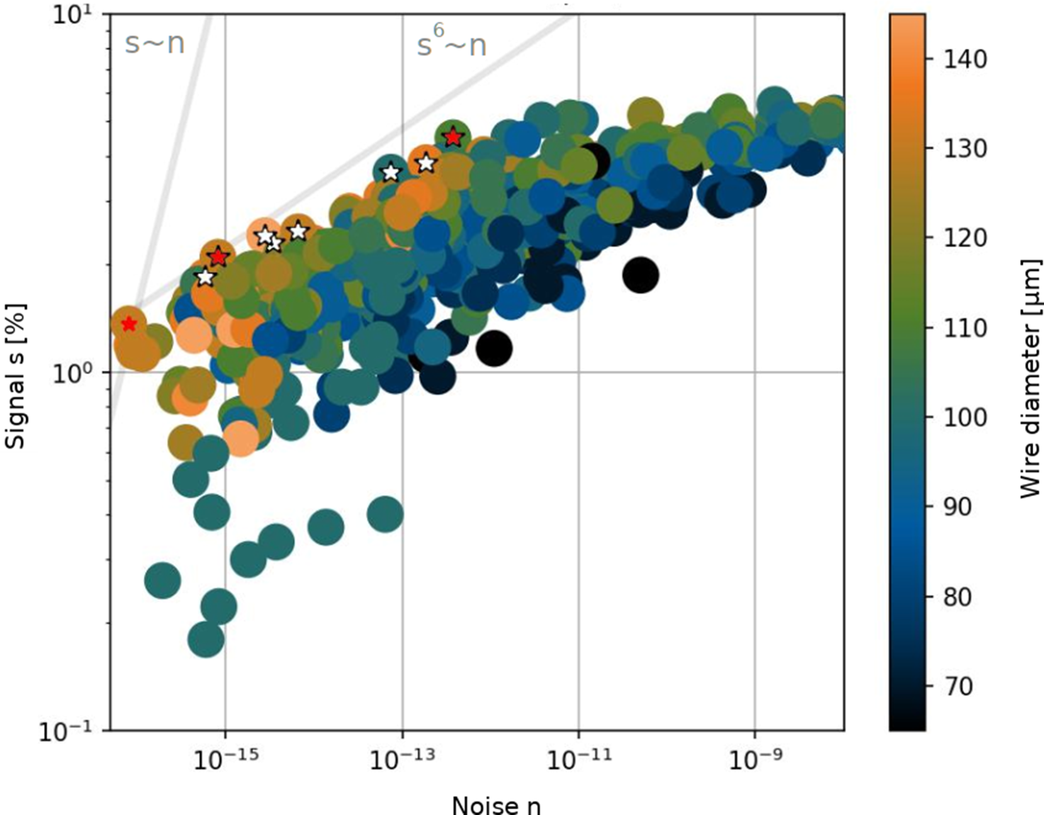
Figure 17 Example of optimization of the experimental parameters. The horizontal axis is the shadow factor, while the vertical one is the signal transmission factor. The diameter of the wire (obstacle O1) is encoded in the colour of the points.
4.2.2 Obstacles
As basic types of obstacles will be round wires, the diffraction and scattering on the edges of the wires are critical. Thus, their surfaces shall be polished to high surface quality, either by focused ion beam (FIB) or electrochemical etching. Commercially available diameters of 200 and $175\kern0.22em \unicode{x3bc} \mathrm{m}$
will be used and simulations have confirmed that the diameter of O2 shall be smaller than that of O1.
$175\kern0.22em \unicode{x3bc} \mathrm{m}$
will be used and simulations have confirmed that the diameter of O2 shall be smaller than that of O1.
Alternatively, a custom-made microfabricated shape was developed to minimize the diffraction and was produced with electroplating. This method uses a focused laser or electron beam to create the desired shape from bulk silicon. Afterwards, nickel is deposited through electroplating. The so-called trumpet shape obtained in this way exhibits a quadratic increase of thickness as a function of decreasing distance from the axis, which transfers to an exponential increase of its opacity. Therefore, as the tip of such a shape is very thin, given by the manufacturing possibilities of the order of a single $\unicode{x3bc} \mathrm{m}$
, the diffraction on such a tip is very limited. On the other hand, the close-to-transparent edge might cause a significant refraction effect, which diverts the photons away from the axis, and therefore such photons do not propagate further downstream and do not contribute to the noise on the detector.
$\unicode{x3bc} \mathrm{m}$
, the diffraction on such a tip is very limited. On the other hand, the close-to-transparent edge might cause a significant refraction effect, which diverts the photons away from the axis, and therefore such photons do not propagate further downstream and do not contribute to the noise on the detector.
A variant of such an object is depicted in Figure 18. The left-hand pane shows the thickness profile as a function of radial distance. The profile is symmetrical, only positive values are shown and are in a wire-like geometry, that is, extended over the not shown dimension. The second and third subplots show the calculated absorption and phase shift caused by the obstacle.

Figure 18 Design of microfabricated obstacles. The left-hand pane shows their shape (thickness as a function of position perpendicular to beam), while the other two panes show the transmission and phase shift induced to the XFEL beam, the combined effect of which is to deflect the beam on the edges rather than to scatter it.

Figure 19 Diffraction simulation of various openings of the slits of apertures A1 and A2 while using the wires as obstacles. The first two figures show the simulated shadow and transmission factors, while the bottom figures show derived $\mathcal{S}/{T}^2$
and
$\mathcal{S}/{T}^2$
and $\mathcal{S}/{T}^6$
factors, which are considered for optimization. Minimum values of the latter factors are desirable for our purpose.
$\mathcal{S}/{T}^6$
factors, which are considered for optimization. Minimum values of the latter factors are desirable for our purpose.
4.2.3 Performance evaluation
Once a set of all beamline elements is given, it is still not trivial to find the optimal settings for the opening of both apertures A1 and A2. Opening of each aperture has its optimal value, which could not be independent of the other one. In general, if an aperture is open too wide, a significant amount of scattered radiation can go through, while if it is closed too much, the signal transmission is decreased and, eventually, additional scattering on the slit edge can be produced. Therefore, a set of simulations for various openings is performed for a given set of components. Figure 19 shows the simulated $\mathcal{S}$
and
$\mathcal{S}$
and $T$
factors in the top row, and the derived quantities
$T$
factors in the top row, and the derived quantities $\mathcal{S}/{T}^2$
and
$\mathcal{S}/{T}^2$
and $\mathcal{S}/{T}^6$
in the second row, for the case in which both O1 and O2 are tungsten wires with respective diameters of 200 and
$\mathcal{S}/{T}^6$
in the second row, for the case in which both O1 and O2 are tungsten wires with respective diameters of 200 and $175\kern0.22em \unicode{x3bc} \mathrm{m}$
. The best performance, that is, the minimum value, of
$175\kern0.22em \unicode{x3bc} \mathrm{m}$
. The best performance, that is, the minimum value, of $\mathcal{S}/{T}^6=2\times {10}^{-4}$
is achieved for openings of 150 and
$\mathcal{S}/{T}^6=2\times {10}^{-4}$
is achieved for openings of 150 and $80\kern0.22em \unicode{x3bc} \mathrm{m}$
, respectively. A different size of A1 increases this factor significantly, while A2 does not have that strong an influence, showing that the majority of signal reduction is done on the O1–A1 pair, while the O2–A2 pair plays rather a minor role.
$80\kern0.22em \unicode{x3bc} \mathrm{m}$
, respectively. A different size of A1 increases this factor significantly, while A2 does not have that strong an influence, showing that the majority of signal reduction is done on the O1–A1 pair, while the O2–A2 pair plays rather a minor role.
This effect is seen even more strongly in simulations with optimized O1–A1 components, as seen in Figure 20. Here, the trumpet shape for O1 is used, and A1 is used with the soft edges of W slits with a plastic phase corrector. By this approach, we improve the best-simulated value for $\mathcal{S}$
by a factor of approximately/almost equal to 30, and the value for
$\mathcal{S}$
by a factor of approximately/almost equal to 30, and the value for $\mathcal{S}/{T}^6$
by a factor of approximately/almost equal to 20. What is interesting is to see that this value is for an A2 size of
$\mathcal{S}/{T}^6$
by a factor of approximately/almost equal to 20. What is interesting is to see that this value is for an A2 size of $300\kern0.22em \unicode{x3bc} \mathrm{m}$
, and is essentially not changing if the aperture is opened more, showing that the cleaning on the first set of components is so superior, that the O2–A2 set does not produce any improvement.
$300\kern0.22em \unicode{x3bc} \mathrm{m}$
, and is essentially not changing if the aperture is opened more, showing that the cleaning on the first set of components is so superior, that the O2–A2 set does not produce any improvement.

Figure 20 Diffraction simulation of various openings of the slits of apertures A1 and A2 while using the trumpet as obstacle O1 and the phase-corrected aperture as A1.

Figure 21 Integrated reflectivity of the considered crystal cuts. For each crystal cut we in addition depict the value of $I{\omega}^2$
in arbitrary units.
$I{\omega}^2$
in arbitrary units.
4.2.4 Ge analyser
As mentioned above, the advantage of the dark-field scheme relies on combining two methods to distinguish the LbL scattered photons from the non-scattered (direct) XFEL photons, the angular scattering and the change of polarization. The set of obstacles and apertures is performing the angular selection, while the second one is yet to be done by a polarization analyser. The main requirements when designing an analyser for these setups were identified as follows:
-
(i) bandwidth covering the majority of the XFEL spectrum;
-
(ii) possibility to measure both polarization states.
As we are relying on crystal-based polarizers, where the setting of the Bragg angle to 45° ensures reflection of only the s-polarization, we have to admit that, to our knowledge, all considered crystal reflections in their default configuration have insufficient bandwidth, that is, they are below or at $0.2\kern0.22em \mathrm{eV}$
, while the bandwidth of the self-seeded XFEL is of the order of
$0.2\kern0.22em \mathrm{eV}$
, while the bandwidth of the self-seeded XFEL is of the order of $1\kern0.22em \mathrm{eV}$
.
$1\kern0.22em \mathrm{eV}$
.
This is pushing the design to use asymmetrical cut crystals, where the angle of incidence is not equal to the Bragg angle. In this configuration, the bandwidth can be significantly improved without losing much of the peak reflectivity, and therefore also the integrated reflectivity is increased. A summary of the performance of considered or common crystals is shown in Figure 21, where the integrated reflectivity is plotted as a function of photon energy, where the given plane can serve as a polarizer. However, it is important to realize that for the success of the vacuum birefringence experiment, the quantity $I{\omega}^2$
, where
$I{\omega}^2$
, where $I$
is the integrated reflectivity (approximated as peak reflectivity times Darwin width) and
$I$
is the integrated reflectivity (approximated as peak reflectivity times Darwin width) and $\omega$
is the probe photon energy, is a good indicator for a suitable crystal, as the number of scattered photons scales as
$\omega$
is the probe photon energy, is a good indicator for a suitable crystal, as the number of scattered photons scales as ${\omega}^2$
. The data points in Figure 21 labelled as assym are those used with asymmetrical cuts with various degrees of asymmetry. That clearly shows that either the Ge 440 or Ge 335 in asymmetrical cuts is the crystals of choice. From those the Ge 440 was chosen, which fixes the experimental constraint to
${\omega}^2$
. The data points in Figure 21 labelled as assym are those used with asymmetrical cuts with various degrees of asymmetry. That clearly shows that either the Ge 440 or Ge 335 in asymmetrical cuts is the crystals of choice. From those the Ge 440 was chosen, which fixes the experimental constraint to $8766\kern0.22em \mathrm{eV}$
. Various cuts and their integrated reflectivities are summarized in Table 5. Theoretically, it is clearly better to employ shallower incidence, which however requires a larger crystal surface with perfect quality. Therefore, various crystals with different cuts are being used for the upcoming experimental campaign, to find which will perform best in given experimental conditions.
$8766\kern0.22em \mathrm{eV}$
. Various cuts and their integrated reflectivities are summarized in Table 5. Theoretically, it is clearly better to employ shallower incidence, which however requires a larger crystal surface with perfect quality. Therefore, various crystals with different cuts are being used for the upcoming experimental campaign, to find which will perform best in given experimental conditions.
Table 5 Parameters of different cuts of Ge 440 crystal reflection.
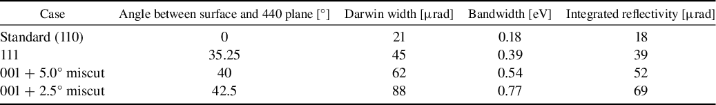
The second condition – the possibility to measure both polarization states – could be easily fulfilled by employing a thin transmissive crystal, as is done in other spectrometers already used, for example, at the HED instrument[
Reference Zastrau, Appel, Baehtz, Baehr, Batchelor, Berghäuser, Banjafar, Brambrink, Cerantola, Cowan, Damker, Dietrich, Di Dio Cafiso, Dreyer, Engel, Feldmann, Findeisen, Foese, Fulla-Marsa, Göde, Hassan, Hauser, Herrmannsdörfer, Höppner, Kaa, Kaever, Knöfel, Konôpková, García, Liermann, Mainberger, Makita, Martens, McBride, Möller, Nakatsutsumi, Pelka, Plueckthun, Prescher, Preston, Röper, Schmidt, Seidel, Schwinkendorf, Schoelmerich, Schramm, Schropp, Strohm, Sukharnikov, Talkovski, Thorpe, Toncian, Toncian, Wollenweber, Yamamoto and Tschentscher
145
]. However, two issues arise if that were to be used in the asymmetric (shallow Bragg angle) geometry: the crystal would have to be extremely thin, and its surface would have to be very precise along a large area. A combination of these two constraints leads us to the conclusion that such precision is not feasible. Therefore, the so-called Baronova configuration[
Reference Baronova, Stepanenko and Stepanenko
146
] is employed, which utilizes a thick crystal in reflective geometry, but in such a geometry that both polarization states are reflected on different planes, and therefore in different directions. This setup will be adopted at the XFEL such that the native XFEL polarization (horizontal) will be reflected above the beam, while the polarization-flipped photons will be reflected horizontally to another camera. The reflectivities for both beams shall be in the predicted value of about $50\kern0.22em \unicode{x3bc} \mathrm{rad}$
.
$50\kern0.22em \unicode{x3bc} \mathrm{rad}$
.
5 Conclusions and outlook
The HED-HIBEF facility at the EuXFEL offers a unique opportunity for the exploration of fundamental properties of the ground state of nature. From a microscopic viewpoint, HED-HIBEF has access to a parameter range of sufficiently large CM energy and photon number density to measure the LbL scattering cross-section, which is induced by quantum fluctuations of QED degrees of freedom. From an effective macroscopic viewpoint, HED-HIBEF can create sufficiently strong fields to discover a nonlinear response of the quantum vacuum, violating the classical superposition principle and providing the vacuum with medium-like properties.
The experiment planned by the present collaboration aims at the discovery of vacuum birefringence, taking advantage of several recent developments: in addition to the HED-HIBEF facility reflecting the progress in generation and control of ultra-intense NIR and X-ray pulses, our concept draws from the evolution of X-ray optics, most prominently high-purity polarimetry, as well as novel theoretical tools for the prediction of quantum signatures generated by generic spatiotemporal pulse distributions.
Because of the diminutiveness of the expected signal, our collaboration envisages several prospective scenarios designed to isolate the nonlinear quantum signature from the expected large linear background. Firstly, beamtime will be used to pursue the dark-field scenario where the discovery potential hinges on the shadow factor $\mathcal{S}$
in combination with X-ray polarimetry as a measure for the quality of background suppression. Currently available facility parameters together with theory predictions, diffractive simulations and practical feasibility suggest this scenario for a first step. However, unforeseen obstacles or improvements in other crucial experimental parameters may subsequently give preference to one of the other scenarios brought forward by our collaboration.
$\mathcal{S}$
in combination with X-ray polarimetry as a measure for the quality of background suppression. Currently available facility parameters together with theory predictions, diffractive simulations and practical feasibility suggest this scenario for a first step. However, unforeseen obstacles or improvements in other crucial experimental parameters may subsequently give preference to one of the other scenarios brought forward by our collaboration.
The first discovery of vacuum birefringence would be a landmark for several reasons: within QED, vacuum birefringence and CMV are genuine prediction similar to phenomena such as the Lamb shift or the anomalous magnetic moment of the electron. In the same measuring manner as the latter to increasing precision, vacuum birefringence should be studied in full detail, because precision experiments provide stringent tests of our understanding of nature, each one coming with its own discovery potential for unexpected deviations.
Vacuum birefringence gives direct access to the HE effective action. For instance, the dark-field scenario and the three-beam setup can measure the two HE coefficients ${c}_1$
and
${c}_1$
and ${c}_2$
separately. This makes these types of experiments an ideal laboratory for investigating effective actions more generally. The fact that effective actions are used for effective field theories in modern physics ubiquitously, for example, in particle physics[
Reference Weinberg
147
, Reference Georgi
148
], solid-state physics[
Reference Zhang, Hansson and Kivelson
149
, Reference Shankar
150
], cosmology[
Reference Cheung, Creminelli, Fitzpatrick, Kaplan and Senatore
151
, Reference Carrasco, Hertzberg and Senatore
152
], searches for hypothetical new physics[
Reference Brivio and Trott
153
, Reference Fitzpatrick, Haxton, Katz, Lubbers and Xu
154
] and even in quantum gravity[
Reference Buchbinder, Odintsov and Shapiro
155
, Reference Donoghue
156
], with the HE action establishing this important concept for the first time makes systematic studies very desirable. In the present context of strong-field QED, the effective action can be studied below and – for increasing probe photon energy – near the mass threshold.
${c}_2$
separately. This makes these types of experiments an ideal laboratory for investigating effective actions more generally. The fact that effective actions are used for effective field theories in modern physics ubiquitously, for example, in particle physics[
Reference Weinberg
147
, Reference Georgi
148
], solid-state physics[
Reference Zhang, Hansson and Kivelson
149
, Reference Shankar
150
], cosmology[
Reference Cheung, Creminelli, Fitzpatrick, Kaplan and Senatore
151
, Reference Carrasco, Hertzberg and Senatore
152
], searches for hypothetical new physics[
Reference Brivio and Trott
153
, Reference Fitzpatrick, Haxton, Katz, Lubbers and Xu
154
] and even in quantum gravity[
Reference Buchbinder, Odintsov and Shapiro
155
, Reference Donoghue
156
], with the HE action establishing this important concept for the first time makes systematic studies very desirable. In the present context of strong-field QED, the effective action can be studied below and – for increasing probe photon energy – near the mass threshold.
As the nonlinear response of the vacuum is a result of quantum fluctuations of all interacting degrees of freedom, the CMV ${k}_{\mathrm{CMV}}$
is not only determined by electron–positron fluctuations. To the lowest order in the coupling constant, all charged degrees of freedom contribute as a matter of principle. However, since
${k}_{\mathrm{CMV}}$
is not only determined by electron–positron fluctuations. To the lowest order in the coupling constant, all charged degrees of freedom contribute as a matter of principle. However, since ${k}_{\mathrm{CMV}}\sim 1/{m}^4$
, the contributions of the next-to-lightest charged particles, muons and charged pions, with masses above
${k}_{\mathrm{CMV}}\sim 1/{m}^4$
, the contributions of the next-to-lightest charged particles, muons and charged pions, with masses above $100\kern0.1em \mathrm{MeV}$
, are suppressed by 9–10 orders of magnitude, presumably interfering with the QED contributions beyond the four-loop level. In contrast to high-energy collider-type experiments, the discovery potential of quantum vacuum experiments extends to the regime of small masses but possibly weakly coupled degrees of freedom[
Reference Gies
157
, Reference Jaeckel and Ringwald
158
].
$100\kern0.1em \mathrm{MeV}$
, are suppressed by 9–10 orders of magnitude, presumably interfering with the QED contributions beyond the four-loop level. In contrast to high-energy collider-type experiments, the discovery potential of quantum vacuum experiments extends to the regime of small masses but possibly weakly coupled degrees of freedom[
Reference Gies
157
, Reference Jaeckel and Ringwald
158
].
In fact, already the first cavity-based experiment, BFRT , searching for vacuum birefringence as well as vacuum dichroism, produced limits on hypothetical small-mass scalar or pseudoscalar degrees of freedom[ Reference Semertzidis, Cameron, Cantatore, Melissinos, Rogers, Halama, Prodell, Nezrick, Rizzo and Zavattini 159 ] and their potential coupling to photons. By now, the set of hypothetical particles – often put forward as dark-matter candidates – that can be searched for in quantum vacuum experiments includes (pseudo-)scalar axion-like particles, scalar or fermionic minicharged particles and additional light vector bosons; see, for example, Refs. [Reference Ahlers, Gies, Jaeckel, Redondo and Ringwald160, Reference Ahlers, Gies, Jaeckel, Redondo and Ringwald161] for a corresponding analysis of the published PVLAS data. In principle, probe photons exposed to a strong field can also mix with neutrinos or gravitons, inducing a tiny standard-model background for vacuum dichroism[ Reference Raffelt and Stodolsky 162 – Reference Ahlers, Jaeckel and Ringwald 164 ].
The strongest bounds on the set of hypothetical particles typically come from astrophysics or cosmology, since such extra degrees of freedom can contribute to heat or photon transport and thus modify generic time or length scales subject to astrophysical observations. However, such bounds often rely on further (stellar or cosmological) model input[ Reference Baker, Cantatore, Cetin, Davenport, Desch, Döbrich, Gies, Irastorza, Jaeckel, Lindner, Papaevangelou, Pivovaroff, Raffelt, Redondo, Ringwald, Semertzidis, Siemko, Sulc, Upadhye and Zioutas 24 , Reference Jaeckel, Masso, Redondo, Ringwald and Takahashi 165 , Reference Hoof, Jaeckel and Thormaehlen 166 ], justifying independent purely laboratory-based experiments as provided by vacuum response measurements.
The search potential of the vacuum birefringence measurement at HED-HIBEF depends on both the hypothetical model degrees of freedom as well as on the details of the measurement scenario. Compared to earlier experiments providing laboratory bounds, such as PVLAS, ALPS, or OSQAR[
Reference Ejlli, Valle, Gastaldi, Messineo, Pengo, Ruoso and Zavattini
78
, Reference Ehret, Frede, Ghazaryan, Hildebrandt, Knabbe, Kracht, Lindner, List, Meier, Meyer, Notz, Redondo, Ringwald, Wiedemann and Willke
167
, Reference Pugnat, Ballou, Schott, Husek, Sulc, Deferne, Duvillaret, Finger, Flekova, Hosek, Jary, Jost, Kral, Kunc, Macuchova, Meissner, Morville, Romanini, Siemko, Slunecka, Vitrant and Zicha
168
], several aspects are different: for example, with reference to Equation (19), our experiment is designed to improve on the flip probability $\sim {I}_{\mathrm{L}}^2{z}^2{\omega}_{\mathrm{X}}^2$
by using an ultra-intense laser with large
$\sim {I}_{\mathrm{L}}^2{z}^2{\omega}_{\mathrm{X}}^2$
by using an ultra-intense laser with large ${I}_{\mathrm{L}}$
and an XFEL with large
${I}_{\mathrm{L}}$
and an XFEL with large ${\omega}_{\mathrm{X}}$
, but at the expense of a small interaction length
${\omega}_{\mathrm{X}}$
, but at the expense of a small interaction length $z$
. Naively, the flip probability for axion-like particles in certain regimes scales as approximately
$z$
. Naively, the flip probability for axion-like particles in certain regimes scales as approximately $\sim {I}_{\mathrm{L}}{z}^2$
for minicharged particles as the QED result for birefringence at small frequencies and as approximately
$\sim {I}_{\mathrm{L}}{z}^2$
for minicharged particles as the QED result for birefringence at small frequencies and as approximately $\sim {I}_{\mathrm{L}}^{2/3}{z}^2/{\omega}_{\mathrm{X}}^{2/3}$
for large frequencies where also dichroism becomes significant, and is even independent of
$\sim {I}_{\mathrm{L}}^{2/3}{z}^2/{\omega}_{\mathrm{X}}^{2/3}$
for large frequencies where also dichroism becomes significant, and is even independent of ${I}_{\mathrm{L}}$
for vector bosons with kinetic mixing.
${I}_{\mathrm{L}}$
for vector bosons with kinetic mixing.
An advantage of HED-HIBEF using an XFEL probe beam is to provide access to mass scales up to the keV regime[ Reference Villalba-Chávez, Podszus and Müller 169 , Reference Evans and Schützhold 170 ], where the bounds of Refs. [Reference Ejlli, Valle, Gastaldi, Messineo, Pengo, Ruoso and Zavattini78, Reference Ehret, Frede, Ghazaryan, Hildebrandt, Knabbe, Kracht, Lindner, List, Meier, Meyer, Notz, Redondo, Ringwald, Wiedemann and Willke167, Reference Astier, Autiero and Baldisseri171] for axion-like particles are rather weak. (Note that bounds in the higher-mass regime[ 172 ] stem from collider experiments and often do not directly measure the axion–photon coupling but rather proceed via its embedding into the electroweak gauge group[ Reference Lees, Poireau and Tisserand 173 ].) Also, enhancements due to resonance effects[ Reference Villalba-Chávez, Podszus and Müller 169 , Reference Evans and Schützhold 170 , Reference Döbrich, Gies, Neitz and Karbstein 174 , Reference Döbrich, Gies, Neitz and Karbstein 175 ] may increase the search potential considerably. We emphasize that further possible advantages arising from the use of, for example, the dark-field scenario relying on the spatiotemporal structure of the field, still remain to be explored.
Let us finally remark that experimental studies of nonlinear vacuum response to strong fields open a new window on fundamental physics probing the parameter space of high amplitude rather than high energy. The scientific potential of this research area has yet to be realized. In a manner analogous to nonlinear media or (relativistic) plasmas for triggering optical phenomena used for a variety of applications, it is conceivable that the quantum vacuum will finally be put to use as the ultimate medium at highest intensities.
Acknowledgements
The authors thank the ExtreMe Matter Institute EMMI at GSI, Darmstadt, for support via an EMMI Collaboration Meeting where this Letter of Intent has been initiated. This work has been funded by the Deutsche Forschungsgemeinschaft (DFG, German Research Foundation) under Grants Nos. 392856280, 416611371, 416607684, 416702141 and 416708866 within the Research Unit FOR2783/2 and Project-ID 278162697 – SFB 1242. AJM is supported by the project ‘Advanced Research Using High Intensity Laser Produced Photons and Particles’ (ADONIS) CZ.02.1.01/0.0/0.0/16_019/0000789 from the European Regional Development Fund (ERDF). The authors also thank Guido Zavattini (PVLAS) as well as Daniel Brandenburg and Frank Geurts (STAR) for their kind permission to reproduce Figures 5 and 6(b).


 Open access