


1. Introduction
Antarctic subglacial hydrology networks are highly sensitive to the surface form of the Antarctic ice sheet (Wright and others, Reference Wright, Siegert, Le Brocq and Gore2008). Changes in ice surface elevation and surface slope throughout glacial cycles have the capacity to significantly change the configuration of ice flow, even in central ice-sheet regions (Siegert and others, Reference Siegert2004) and, because of this, to change subglacial hydrological networks (i.e. subglacial water flow direction, location of subglacial lakes, catchment area, etc.). As key components of subglacial hydrological networks, we can assume that subglacial lakes too may be subject to changes over glacial cycles, including their volume. Subglacial hydrological networks can impact the overlying ice flow by changing the basal friction and ice bottom elevation (Livingstone and others, Reference Livingstone2022). Subglacial drainage has also been shown to modulate the basal melting pattern of ice shelves (e.g. Wei and others, Reference Wei2019; Pelle and others, Reference Pelle, Greenbaum, Dow, Jenkins and Morlighem2023). Understanding the close interaction between ice sheets and subglacial hydrology systems is, therefore, critical for accurately simulating the behavior of ice sheets and ice shelves throughout glacial cycles in order to understand ice-sheet evolution.
Recent airborne geophysical surveys coordinated by the second International Collaborative Exploration of the Cryosphere through Airborne Profiling (ICECAP2) initiative confirmed the existence of a large subglacial lake, Lake Snow Eagle (LSE), in the interior of Princess Elizabeth Land (PEL), East Antarctica (Yan and others, Reference Yan2022) (Fig. 1). LSE is located in the upstream part of an extensive subglacial canyon network, whose orientation is orthogonal to the ice-flow direction near LSE and likely connects to the coastal area of PEL (as estimated by Jamieson and others (Reference Jamieson2016) based on satellite-based observation of the ice surface, assuming the large-scale feature on the ice surface reflects subglacial topography) (Fig. 1). Such subglacial channels could serve as efficient subglacial water pathways, making LSE potentially connected to the surrounding and downstream subglacial hydrology networks. Therefore, the drainage of LSE could influence the downstream subglacial hydraulic conditions and impact the flow dynamics of the downstream ice.
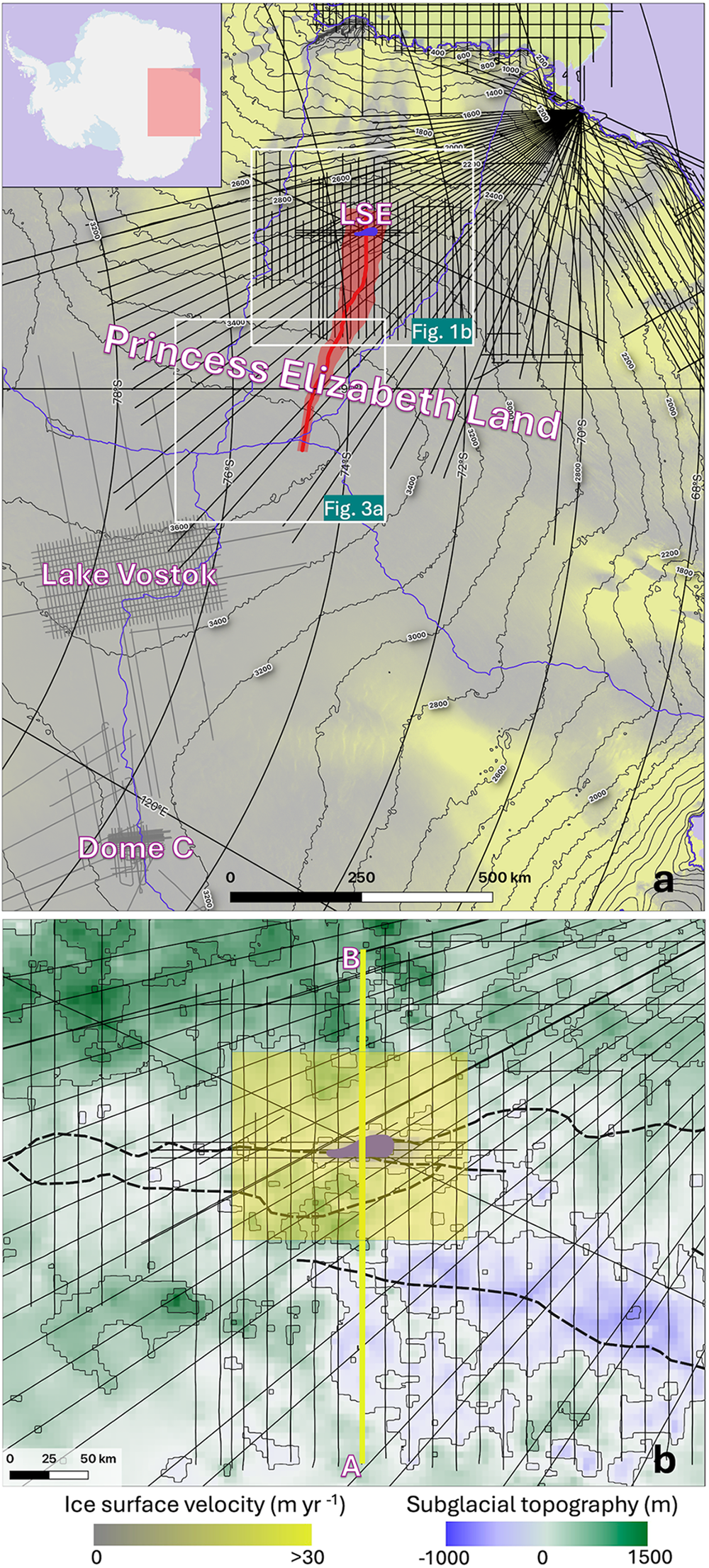
Figure 1. Map of the study area. (a) Surface elevation and velocity map. The background color shows the ice-flow speed from MEaSUREs InSAR-Based Antarctic Ice Velocity Map, Version 2 (Rignot and others, Reference Rignot, Mouginot and Scheuchl2017). Blue lines mark the location of ice divides (Zwally and others, Reference Zwally, Giovinetto, Beckley and Saba2012). Surface elevation contours are shown in thick gray lines (Jezek and others, Reference Jezek, Curlander, Carsey, Wales and Barry2013). The red line marks the location of the flowline used for the ice-flow model, while the red shade marks the flowband width, both based on the surface velocity data from MEaSUREs InSAR-Based Antarctic Ice Velocity Map, Version 2 (Rignot and others, Reference Rignot, Mouginot and Scheuchl2017). Black lines show the location of airborne geophysical survey collected in Princess Elizabeth Land (Cui and others, Reference Cui2020), while thin gray lines show the location of preexisting airborne geophysical dataset in the Lake Vostok and Dome C areas (Young and others, Reference Young2017; Frémand and others, Reference Frémand2023). The location of LSE is marked by the blue area (Yan and others, Reference Yan2022). The map at up-left shows the overall location of this map. The location of panel (b) and Figure 3a are marked by white rectangles. (b) Subglacial topography of the LSE area. The background color shows the subglacial topography of the LSE area, as measured by airborne radio-echo sounding survey (Cui and others, Reference Cui2020). Subglacial topography contour has intervals of 250 m (thin) and 1000 m (thick). The black lines show the location of the airborne geophysics survey collected in the area through the ICECAP2 initiative (Cui and others, Reference Cui2020). The location of LSE is marked by the blue area (Yan and others, Reference Yan2022). Thick blue dash line shows the location of the subglacial canyon network, estimated from satellite-based remote-sensing (Jamieson and others, Reference Jamieson2016). The thick yellow line highlights the location of the radargram shown in Figure 2. The yellow square marks the location of the map shown in Figure 4.
Geophysical inversion of airborne gravity data collected by ICECAP2 indicates the existence of a sediment layer up to over 200 m thick at the bottom of LSE (Yan and others, Reference Yan2022). Given the low expected sedimentation rate, such a substantial sediment layer likely holds a valuable and rarely available record of geological and environmental changes in the interior of East Antarctica (Kennicutt and others, Reference Kennicutt2019; Yan and others, Reference Yan2022). One critical reference for future analysis and interpretation of this sediment record is the past evolution of LSE; for example, the draining and refilling of lake water and changes in the catchment area. Because the migration of subglacial water (i.e. subglacial lake drainage and filling events) could induce localized changes in ice surface elevation, such events can be monitored by satellite observations if the water drainage volume is large enough (e.g. Fricker and others, Reference Fricker, Scambos, Bindschadler and Padman2007). One approach to constraining these observations prior to the satellite record is to directly access these sediments to observe laminations (Siegfried and others, Reference Siegfried2023); however, at a depth of over 3.5 km, LSE is a challenging target for access and sampling, and without expected radiogenic, biological or satellite-detected elevation change constraints on timing, a sediment-based approach alone would seem difficult.
Fortunately, englacial radiostratigraphy can retain valuable information about the history of the ice sheet including past ice-flow reconfiguration (e.g. Beem and others, Reference Beem2018), paleo-accumulation patterns (e.g. Waddington and others, Reference Waddington, Neumann, Koutnik, Marshall and Morse2007; Leysinger Vieli and others, Reference Leysinger Vieli, Hindmarsh, Siegert and Bo2011; Cavitte and others, Reference Cavitte2018) and basal melting patterns (e.g. Ross and Siegert, Reference Ross and Siegert2020). In particular, time-varying boundary conditions experienced over limited parts of the ice sheet, for example transitions from frozen to melting at the bed, may be imprinted on layer shapes. Therefore, englacial stratigraphy offers a unique opportunity to gain insight on the past evolution of LSE. In this study, we combine the englacial radiostratigraphy in the LSE area with a numerical ice-flow model that simulates englacial stratigraphy to investigate the hydrological evolution of LSE. Such knowledge is important for understanding the sedimentary record within LSE and, more broadly, past changes in the PEL sector of the East Antarctic ice sheet.
2. Methods
2.1. Airborne ice-penetrating radar sounding and englacial stratigraphy
Ice-penetrating radar systems have been used to advance our understanding of the cryosphere for over five decades (see Schroeder and others (Reference Schroeder2020) and references therein). Such radar systems provide high-resolution measurements of subglacial topography and ice sheet thickness (e.g. Cui and others, Reference Cui2020), as well as valuable insights on englacial structure and subglacial hydraulic conditions (e.g. Schroeder and others, Reference Schroeder, Blankenship and Young2013; Beem and others, Reference Beem2018; Yan and others, Reference Yan2022) (Figs 2, S1 and S2). The airborne survey platforms deployed in ICECAP2 seasons are equipped with an ice-penetrating radar based on the HiCARS2 system developed by University of Texas Institute for Geophysics, which is a coherent, 60-MHz ice-penetrating radar system with 15 MHz of bandwidth (Peters and others, Reference Peters, Blankenship and Morse2005; Young and others, Reference Young2011; Cui and others, Reference Cui2018). After pulse-compression and synthetic aperture radar (SAR) processing (Peters and others, Reference Peters, Blankenship, Carter, Kempf, Young and Holt2007), this system provides a vertical resolution of 8.5 m in ice and an along-track resolution of 44 m (Cavitte and others, Reference Cavitte2018). The radar data used in this study were collected in PEL over four field campaigns (2016–19) through the ICECAP2 initiative. To expand the stratigraphic chronology of the region, these radar surveys were designed to connect to the preexisting radar datasets with internal layers dated from ice-core intersections in the Lake Vostok and Dome C regions (Fig. 1).
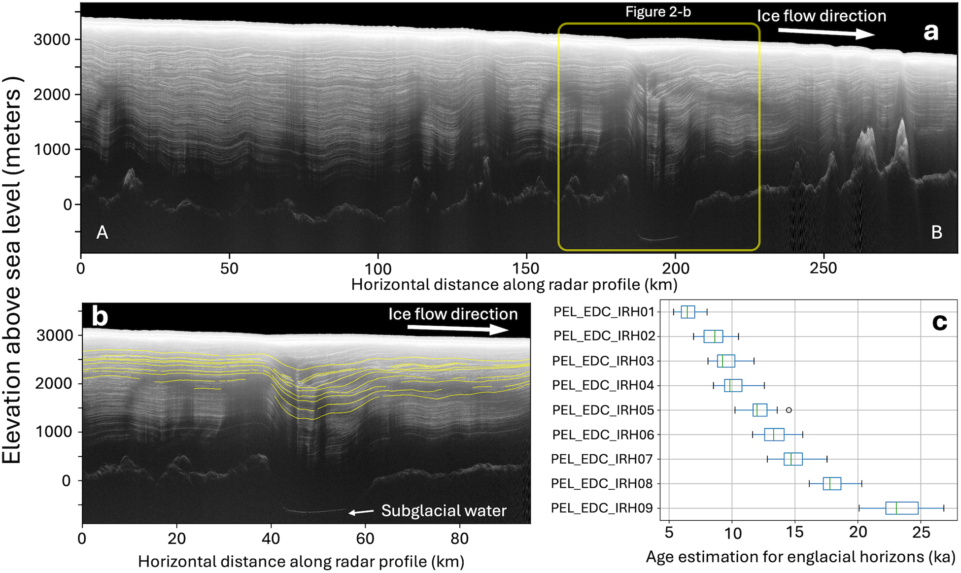
Figure 2. Englacial radio-stratigraphy above LSE. (a) Example radargram collected through the LSE area. The location and orientation of this radargram is marked in Figure 1. Additional radargrams collected through the LSE area can be found in the Supplementary Materials (Figs S1 and S2). (b) A zoom-in view of the stratigraphic disruption above LSE, whose location is marked in panel (a). Yellow lines show the nine traced englacial reflections in the LSE area, with PEL_EDC_IRH01 being the shallowest (closest to the ice surface) and PEL_EDC_IRH09 being the deepest. (c) Age estimation of the nine traced englacial reflections in the LSE area. All elevation data shown in this manuscript are relative to the WGS84 ellipsoid.
In this study, we use internal reflecting horizons (IRHs) to infer past evolution of the ice sheet. IRHs in ice-penetrating radar sounding are caused by variations in electric conductivity and permittivity across the ice column, due to changes in ice fabric, density and acidity (Wrona and others, Reference Wrona, Wolovick, Ferraccioli, Corr, Jordan and Siegert2018; Bingham and others, Reference Bingham2024). Continuous IRHs are generally considered isochronous (i.e. resulting from layers of snow deposited on the ice sheet surface around the same time) (e.g. Eisen and others, Reference Eisen, Wilhelms, Steinhage and Schwander2006; Ashmore and others, Reference Ashmore, Bingham, Ross, Siegert, Jordan and Mair2020; Elsworth and others, Reference Elsworth, Schroeder and Siegfried2020). Nine IRHs of interest in the LSE area (referred to as PEL_EDC_IRH01-09) are traced using the DecisionSpace Geosciences 10ep software package (Figs 2, S1 and S2), which contains semiautomatic tracing algorithms and enables continuous IRHs tracing across transects (Cavitte and others, Reference Cavitte2021). These nine IRHs are selected because they cover the depth range where a disruption in the englacial stratigraphy is observed, as well as their overall continuity. While a series of additional reflections are also visible in the deeper portion of the ice column, those reflections are vulnerable to disruptions when the ice flows over rough terrain and are therefore largely discontinuous and difficult to trace. The thickness of ice units between traced IRHs are then calculated assuming a constant electromagnetic velocity of 168.5 m µs−1 in ice (Cavitte and others, Reference Cavitte2016).
In addition to the aforementioned nine IRHs traced in the LSE area, we extend six of the dated IRHs in Cavitte and Others (Reference Cavitte2021) from the Dome C area to PEL, which were dated by referencing the AICC2012 chronology (Bazin and others, Reference Bazin2013; Veres and others, Reference Veres2013) (Fig. 3b). With these dated IRHs providing a reference, and assuming the age of 0 ka (present) for the ice sheet surface, we use the Dansgaard–Johnsen age-depth model to estimate the age of the nine aforementioned undated IRHs traced in the LSE area (Dansgaard and Johnsen, Reference Dansgaard and Johnsen1969). The Dansgaard–Johnsen model is a one-dimensional ice-flow model that assumes a shear layer above the bottom of the ice column capped by a non-shear layer. The horizontal ice-flow velocity in the bottom shear layer is assumed to be proportional to the elevation above bed, while the horizontal ice-flow velocity in the top non-shear layer is assumed to be constant and elevation-independent. Because the thickness of the shear layer is unknown for our study area, we construct four models to represent possible locations for the shear-layer boundary: (1) below the 96 ka reflection, (2) between the 96 ka reflection and the 82 ka reflection, (3) between the 82 ka reflection and the 73 ka reflection and (4) above the 73 ka reflection. Models with different assumptions of shear-layer boundary depth appear to yield similar results, as shown in Fig. 3c.
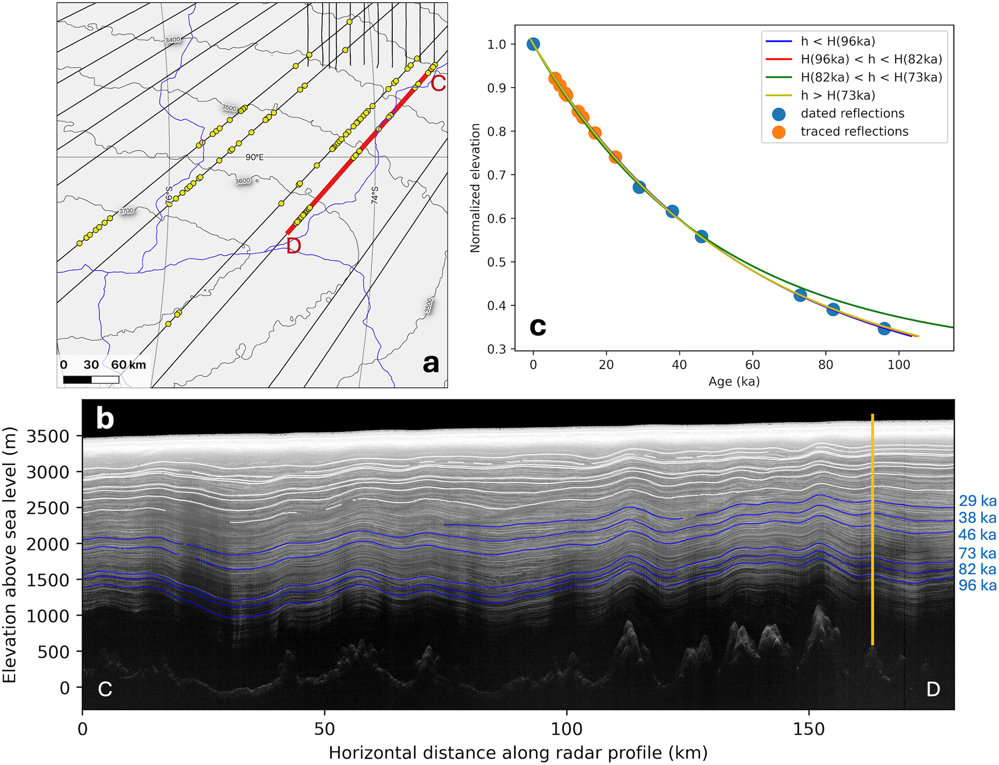
Figure 3. Age estimation of traced IRHs. (a) A map of interior PEL, whose location is marked in Figure 1a. Black lines show the airborne radar transects collected by ICECAP2. Yellow dots show the 91 locations where the Dansgaard–Johnsen model is used to constrain the age-depth profile. Red line highlights the location and orientation of the radargram shown in panel (b). Blue lines mark the location of ice divides (Zwally and others, Reference Zwally, Giovinetto, Beckley and Saba2012). Surface elevation contours are shown in thick gray lines (Jezek and others, Reference Jezek, Curlander, Carsey, Wales and Barry2013). (b) An example radargram showing the nine undated IRHs traced for the LSE area (white lines) and the six dated IRHs extended from the Dome C area (blue lines, ages are mark on the right-hand side). (c) A comparison between the age-depth curves derived from different assumptions of the basal shear layer thickness (h) at the same location, whose location is marked by the yellow vertical bar in panel (b). h represent the thickness between a certain IRH and the bedrock.
We use the Dansgaard–Johnsen model to constrain the age-depth profile at 91 selected sites in south-eastern PEL (Fig. 3a), the statistics of which is then used to estimate the age of the traced englacial reflections. These locations were selected based on three criteria: (1) most of the traced englacial reflections from the LSE area and dated englacial reflections from the Dome C area are identifiable and continuous; (2) basal roughness is relatively low, which enables us to neglect the influence of rough terrain; and (3) proximity to ice divide. These criteria increase the likelihood that the assumptions underlying the 1-D the Dansgaard–Johnsen model are met.
We acknowledge that the 1-D Dansgaard–Johnsen model is a relatively simple tool for estimating the age-depth profile and relies on several key assumptions about ice-flow conditions. Specifically, this approach involves averaging the surface accumulation rate over the entire time span represented by the ice column. While this simplification provides a first-order estimate of the age of the traced IRHs, it may introduce inaccuracies, particularly in regions where the surface accumulation rate has varied significantly over time. Therefore, if future studies are able to provide constraints on past accumulation rate changes in the study area, incorporating this variability into the age-depth model will be essential for improving the accuracy of age estimations.
2.2. Ice-flow model
In this study, we use a 2.5-D ice-flow forward model that allows for varying boundary conditions to understand the evolution of LSE (Koutnik and Waddington, Reference Koutnik and Waddington2012). This model can simulate the geometry of englacial horizons of prescribed ages, which then can be compared to the observed IRHs. The ice-flow model represents a vertical 2-D cross section of the ice sheet from the surface to the bed, with an additional half dimension accounting for transverse strain rate along the ice-flow direction (Fig. 1a). The model has a limited domain, constrained to the interior of the ice sheet, extending from the upstream ice divide to downstream of LSE where the radar measurement profile ends. By including the upstream ice divide in the model domain, the upstream boundary condition is a zero-flux condition and any influences from the surface and bed conditions upstream are advected to the vicinity of LSE and represented in the simulated stratigraphy.
The model incorporates general information about the full-domain response of the ice sheet through response functions that scale how the limited portion of the ice sheet responds to changes in accumulation and ice flux over time (Koutnik and Waddington, Reference Koutnik and Waddington2012). Boundary conditions for the ice-flow model and the values we prescribe in the model include: (1) bed elevation, which we obtain from measurements by airborne radar sounding (Cui and others, Reference Cui2020); (2) flow band width, accounting for transverse strain rate along the ice-flow direction, which we derive by tracing ice velocity divergence along the ice-flow direction, with ice surface velocity from MEaSUREs InSAR-Based Antarctic Ice Velocity Map, Version 2 (Rignot and others, Reference Rignot, Mouginot and Scheuchl2017); (3) geothermal flux, which is estimated from satellite magnetic data by Maule and others (Reference Maule, Purucker, Olsen and Mosegaard2005); (4) surface accumulation rate (varying spatially between ∼4 and 6 cm yr–1) and mean-annual surface temperature (varying spatially between −40 and −30oC), which were estimated based on values from the RACMO2 model (van Wessem and others, Reference van Wessem Jm2018). In this model study, we assume that the surface elevation has been similar to the modern values over the past 23 ka of the model run.
Our ice-flow model uses the Shallow-Ice Approximation (SIA) to describe the ice-flow field (Cuffey and Paterson, Reference Cuffey and Paterson2010), except that we assume plug flow over LSE when the lake is active with the ice flowing at a column-uniform rate that is less than the surface velocity; the plug-flow velocity over the lake is a tunable parameter. The horizontal resolution of the model is chosen to be 1000 m, which reasonably represents the stratigraphy and is necessarily efficient, and the vertical resolution is nondimensionalized by the ice thickness to be 0.002 (∼5–7 m along the domain when dimensionalized). The time stepping in the model runs is 100 years, but particle tracking through the gridded velocity field is done at finer resolution using an interval stepping of 1000 for all modeled IRHs.
By integrating the modeled velocity field, the paths of ice particles deposited on the surface over time can be used to calculate the englacial stratigraphy. This modeled englacial stratigraphy is then compared with the observed englacial stratigraphy obtained by radar sounding, similar to the iterative evaluation process in Koutnik (Reference Koutnik2016). A more detailed description of the ice-flow model can be found in the Supplementary Materials (Supplementary Note #1).
3. Results
3.1. Englacial stratigraphy over the LSE area
In this study, nine continuous englacial reflections within the top half of the ice column are traced by semiautomatic tracing algorithms across the LSE area and toward south-eastern PEL (Fig. 2), and their age estimations are shown in Table 1.
Table 1. Statistics of age estimation for the traced IRHs in the LSE area
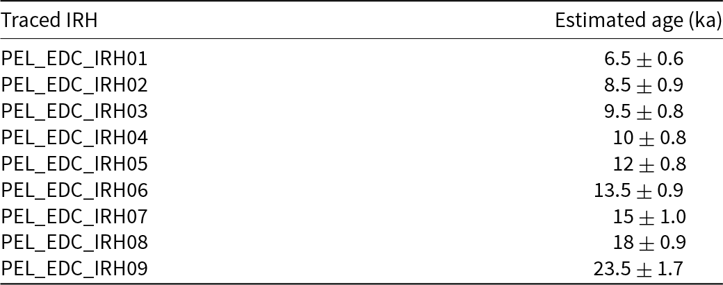
Errors reflect the standard deviation of the Dansgaard–Johnsen model results.
We observe a change in the englacial radio-stratigraphy pattern in the upper ice column over LSE. While the thickness of the ice units between IRHs are relatively constant upstream of LSE (left-hand side in Fig. 2, and grid south in Fig. 4), distinct short spatial wavelength, high amplitude spatial variations in ice unit thickness are present in the upper ice column over LSE (Figs 2 and 4). The most prominent variation is observed in the ice unit whose formation age is estimated to be between 9.5 and 12 ka, where the thickness of this unit varies by more than 150 m across horizontal along-flow distance of 10 km (Fig. 4). The horizontal extent and location of this anomalous thickness variation corresponds well with LSE (Figs 2 and 4), while the thickness of this ice unit stays relatively constant elsewhere in the study area. This anomalous stratigraphic disruption observed above LSE indicates past changes in ice-flow dynamics resulted in such a distinct signature being recorded in the englacial stratigraphy. The strong spatial correspondence between this stratigraphic disruption and LSE implies a connection between ice-flow changes and the subglacial lake.
3.2. Qualitative analysis of the change in englacial stratigraphy over LSE
To investigate the potential processes that may contribute to the observed disruption of englacial stratigraphy in the vicinity of and across LSE described in the previous section, we consider factors and processes that can potentially alter the englacial stratigraphy, including
(a) Subglacial topography. LSE is located inside a subglacial canyon, whose orientation is orthogonal to the regional ice-flow direction (Jamieson and others, Reference Jamieson2016; Yan and others, Reference Yan2022). The canyon’s extreme topographic relief—more than 1000 m over just a few kilometers—can significantly disrupt the ice flow, particularly near the base, and alter the shape of the IRHs. The imprint of subglacial topography on englacial stratigraphy tends to correspond with the along-flow derivative of topography (e.g. Ross and Siegert, Reference Ross and Siegert2020), typically being vertically continuous propagating from bottom upward where the impact has a similar amplitude in adjacent ice layers. The imprint of subglacial topography is also expected to be more pronounced for the IRHs closer to the ice–rock interface compared to the IRHs near the ice surface.
(b) Climate-controlled changes in the rate and pattern of surface accumulation throughout the time span that is covered by the traced IRHs in the LSE area (e.g. Leysinger Vieli and others, Reference Leysinger Vieli, Hindmarsh, Siegert and Bo2011), whose imprint would have a relatively long horizontal span. For example, the reconstructed paleo-accumulation rate at Dome C by Cavitte and others (Reference Cavitte2018) shows variation with a spatial wavelength on the order of hundred kilometers.
(c) Past ice-flow reorganization, whose imprint tends to be horizontally continuous and has a long-spatial-wavelength imprint on the englacial stratigraphy (e.g. Beem and others, Reference Beem2018) and, vertically, can only be observed in the IRHs formed prior to and around the time of the reorganization.
(d) Changes in ice-flow rate due to subglacial water storage that decreases the basal friction in the vicinity of the subglacial water body (e.g. Sergienko and Hulbe, Reference Sergienko and Hulbe2011; Gudlaugsson and others, Reference Gudlaugsson, Humbert, Kleiner, Kohler and Andreassen2016). Similar to factor (a), the imprint from sliding over basal water tends to be vertically continuous, propagating from bottom upwards where its horizontal extent would correlate with the subglacial water body, and is only present when the basal non-friction zone is of a sufficient area (e.g. Sergienko and Hulbe, Reference Sergienko and Hulbe2011; Gudlaugsson and others, Reference Gudlaugsson, Humbert, Kleiner, Kohler and Andreassen2016).
(e) Basal melting and freezing, which can be present at the ice–water interface above subglacial lakes (e.g. Leysinger Vieli and others, Reference Leysinger Vieli, Hindmarsh and Siegert2007; Filina and others, Reference Filina, Blankenship, Thoma, Lukin, Masolov and Sen2008; Leysinger Vieli and others, Reference Leysinger Vieli, Martín, Hindmarsh and Lüthi2018). For the imprint of basal melting and freezing, its horizontal span of IRH shape is confined primarily to the melting/freezing spots (e.g. Ross and Siegert, Reference Ross and Siegert2020), while vertically its imprint can be present across the entire ice column.
(f) Redistribution of surface snowfall by the combination of surface wind and surface slope break (e.g. Grima and others, Reference Grima, Blankenship, Young and Schroeder2014), whose imprint tends to have a short horizontal span that correlates to local changes in surface slope (e.g. Verfaillie and others, Reference Verfaillie2012; Guo and others, Reference Guo2020). Vertically, the imprint would be mostly confined within the IRHs that were formed during the time period when such redistribution was present.
The disruption of englacial stratigraphy above LSE is only present in the upper half of the ice column (Figs 2, 4, S1 and S2). Horizontally, in the along-flow direction, this disruption extends over a similar distance as the along-flow width of LSE and its hosting subglacial canyon, with a span around 10 km (Figs 2, 4, S1 and S2). Across the ice-flow direction, the width of this disruption is comparable to the across-flow width of LSE, which is around 40 km (Figs 2, 4, S1 and S2). After comparing these characteristics against those outlined above for process (a), (b) or (c), it appears that these specific mechanisms are less likely to be the primary driver of the observed disruption. We cannot entirely dismiss their influence, as more complex interactions may still play a role. Fully constraining the impact of these processes, however, is particularly challenging due to the limited understanding of the area’s complex topographic setting and the past changes in ice flow and climate conditions. As the primary goal of this study is to identify the primary cause for the anomalous stratigraphic disruption observed over LSE, we choose to focus on the other potential mechanisms and apply a simplified ice-flow model to quantitatively assess their impact on the englacial stratigraphy, providing a more detailed understanding of the observed stratigraphic disruption.
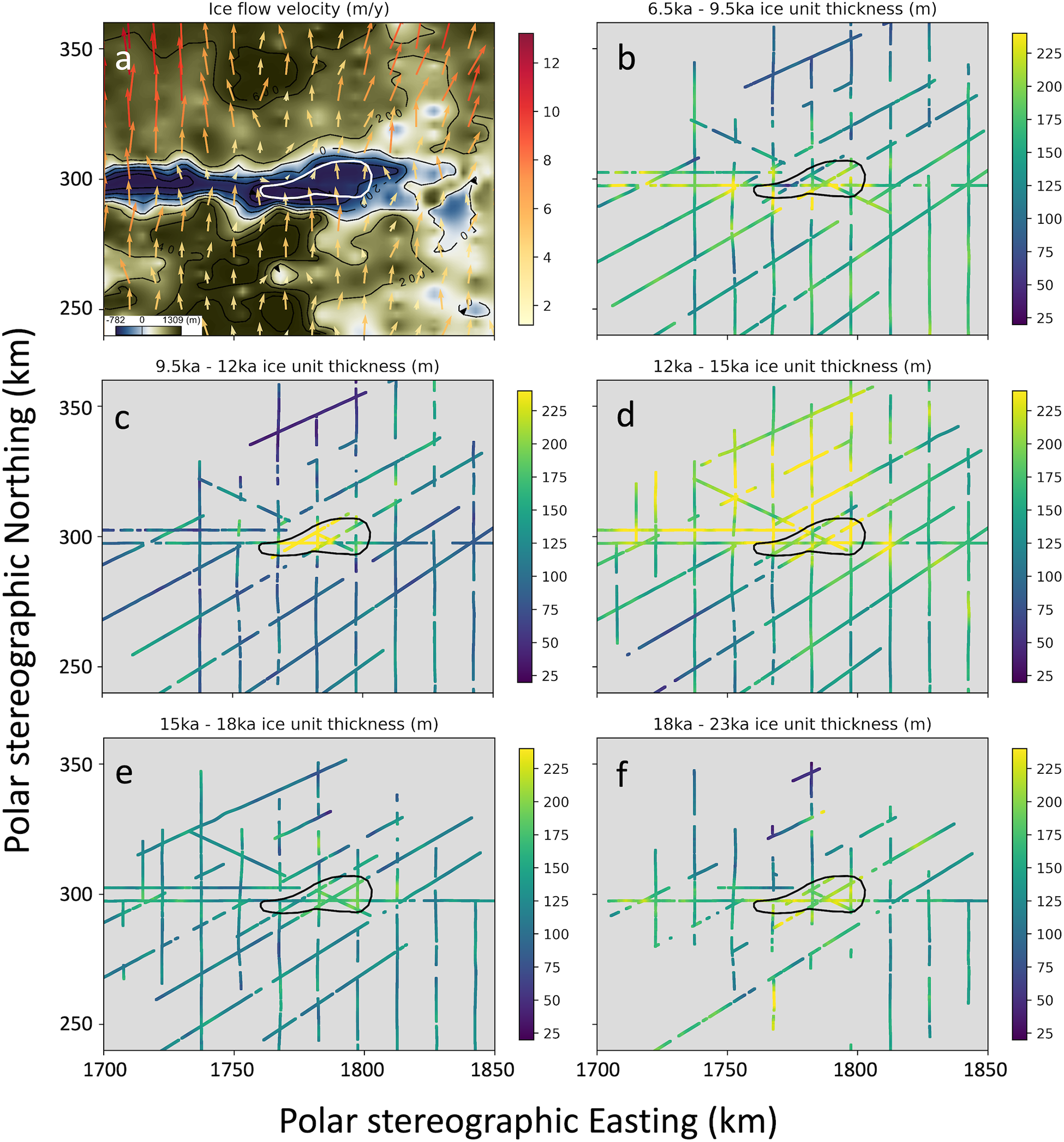
Figure 4. (a) Ice-flow velocity (Rignot and others, Reference Rignot, Mouginot and Scheuchl2017) in the LSE area plotted on a map of radar-derived subglacial topography (Cui and others, Reference Cui2020). Subglacial LSE is shown by a white polygon line. Arrow direction represents ice-flow direction, and arrow color and length represent ice-flow rate. (b–f) Thickness of ice layer unit between englacial reflections of specific ages. The age for each ice unit is labeled in subplot titles. Colorbar shows the layer packet thickness in meters. Subglacial LSE is shown by a black polygon line. Coordinates are in EPSG 3031–WGS 84 / Antarctic Polar Stereographic.
3.3. Quantitative analysis of the irregular englacial stratigraphy at LSE
To systematically investigate the potential source of the irregular stratigraphy, we assess the impact of different processes by tracking how the modeled layers change as a function of combinations of different model-parameter values representing those processes, and compare the modeled IRHs shape and depth to the radar observation.
1. Base model setup
To evaluate the parameter choice and model setup, we first build a ‘base run’ with the modern bed elevation as measured from radar sounding, without water fill of the subglacial canyon, basal melting, basal sliding or surface accumulation redistribution over LSE (Fig 5a and b). The mismatch shown in Fig. 5 is calculated by comparing the modeled depth and the observed depth of each IRH, where positive mismatch means that the modeled IRH is deeper than observed.
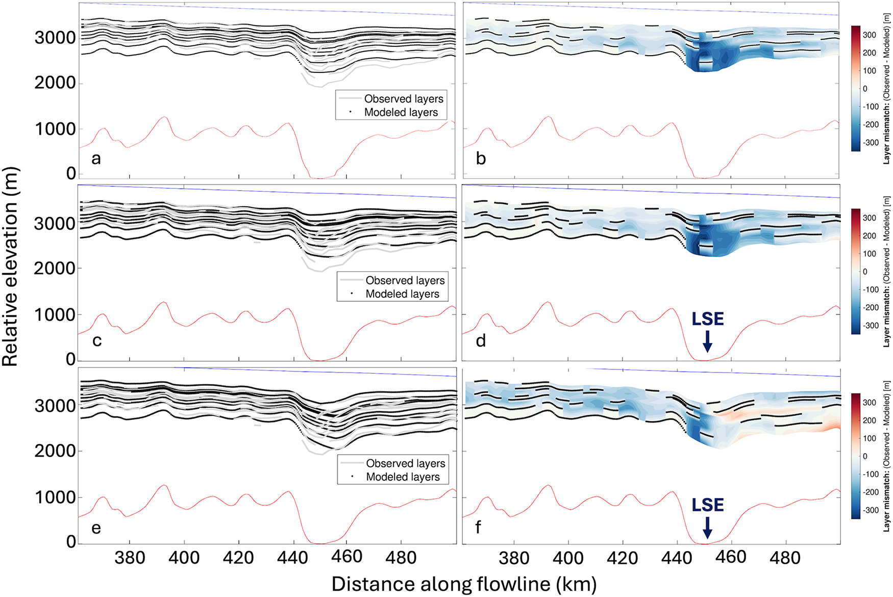
Figure 5. Comparison of the observed and modeled IRHs from different model setups. (a, c and e) Show direct comparisons between the modeled and observed IRHs depth, while (b, d and f) show the mismatch contour. Panels (a and b) are from the base run setup. Panels (c and d) are from the model setup with plug flow and basal melting. Panels (e and f) are from the model setup with surface snow redistribution. Please note that for the base run, we assume no waterfill in the LSE basin and drop the ice bottom for 100 m, which is about the average water depth as estimated by Yan and others (Reference Yan2022). The location of LSE is marked in (d and f). For the mismatch contour plots, blue color means that the observed IRH is deeper than the modeled IRH, and black dots mark the discretized modeled IRHs depth where the traced IRHs depth is absent.
To evaluate model fit, we calculate the root-mean-square (RMS) mismatch between the modeled and observed stratigraphy across the model domain. A lower RMS indicates a better overall fit. Additionally, we need to consider the tolerance value in order to evaluate our model fits, as for this study we seek the minimum mismatch but need to consider that the data have uncertainties. The modeled IRH depth is affected by the inferred IRH age uncertainty. By comparing the depth difference between IRHs with an age difference of around 1 ka, it appears that a reflection age difference of 1 ka induces a depth difference of around 65 m. As the standard deviations for IRH age estimation for most traced IRHs are around 1 ka, we treat this 65-m value as a tolerance for fitting IRHs with our model. We refer to model setups with an RMS mismatch smaller than 65 m as ‘accepted setups’, but we do not rank these ‘accepted setups’ or interpret parameter combinations from a single accepted model. If this was set up as a formal inverse problem, or if additional constraints on the ages of the traced IRHs were available through direct or indirect approaches, we could more rigorously consider data uncertainties and work toward finding the ‘best’ set of model parameters within these uncertainties that avoids overfitting the data (e.g. Gudmundsson, Reference Gudmundsson, Singh, Singh and Haritashya2011). For this study, we seek to constrain characteristics of model setups that minimize the mismatch to the observations, and to support future work that can more robustly evaluate inferences about specific parameters and/or combinations of parameters in a different modeling framework.
For the base model setup, the mismatch RMS across all nine traced IRHs within the shown model domain is 133 m. Upstream of LSE (the left half of the model domain shown in Fig. 5), the mismatch between simulated and observed englacial stratigraphy is within the order of inherited uncertainty from IRH age estimation (65 m), which indicates that the model setup and parameter selection are reasonable. However, above and downstream of the lake, the modeled IRHs are over 300 m shallower than the observation, and the short wavelength variation over the lake in the upper half of the ice column is not produced. This result indicates the need to incorporate additional processes into the model.
2. Impact of basal lubrication and basal melting
Next, we examine the impact of basal lubrication (by existence of a subglacial lake) and basal melting on the englacial stratigraphy. Previous studies have estimated the basal melting rate of other major subglacial lakes to range from centimeters per year to tens of centimeters per year (e.g. Siegert and others, Reference Siegert, Kwok, Mayer and Hubbard2000; Ross and Siegert, Reference Ross and Siegert2020). Since the contemporary basal melt rate of LSE is not constrained, we use this range as a starting point to assess the impact of basal melt on englacial stratigraphy. As a preliminary test, we impose plug flow and a basal melt rate of 0.1 m yr–1 in the model over the location of LSE, and then compare the modeled englacial layers to the observed layers (Fig 5c and d). The mismatch RMS for this model setup is 90 m. The modeled IRHs above LSE are deeper than those in the base run, due to the drawdown effect of basal melting, thereby resulting in a reduced mismatch. However, there remains a mismatch of ∼300 m over LSE, and the observed stratigraphic disruption above LSE is not adequately reproduced. This result indicates that while basal melting is or has been present over LSE, it is not the primary cause for the irregular englacial stratigraphy observed in the upper ice column over LSE.
3. Impact of surface snowfall redistribution
Next, we proceed to explore the potential impact of surface snowfall redistribution that could be present in the LSE area. With a sufficient area of basal lubrication, the impact of basal sliding can propagate through the entire ice column, resulting in a distinctive localized high-amplitude variation of the ice surface slope. Such expression is observed for many major subglacial lakes (e.g. Filina and others, Reference Filina, Blankenship, Thoma, Lukin, Masolov and Sen2008), including LSE (Yan and others, Reference Yan2022) (Figs S8 and S9). While the overall ice surface slope in the area dips toward the grid north-east direction as the ice flows toward the Amery Ice Shelf, a local 20 m depression can be observed over the subglacial lake (Fig. S9). It has been shown that such localized variation of surface slope is capable of redistributing surface snowfall (e.g. Sugiyama and others, Reference Sugiyama2012; Verfaillie and others, Reference Verfaillie2012; Grima and others, Reference Grima, Blankenship, Young and Schroeder2014). More specifically, short wavelength ‘breaks’ in surface slope have been shown to induce a relatively significant increase in surface accumulation rate by redistributing surface snowfall. Both airborne radar sounding surveys and satellite based observations show such a surface feature is present over LSE (Yan and others, Reference Yan2022), which indicates that topographic redistribution of surface snowfall could be present in the LSE area. Additionally, a study conducted by Das (Reference Das2013) identified likely wind scour zones across East Antarctica based on surface slope, where scour zones are identified within 10 km of LSE. This finding suggests snowfall redistribution caused by the combination of wind scour and surface slope is likely present in the vicinity of LSE. Such a localized anomaly in surface accumulation can cause a short-wavelength variation in the ice unit thickness, and the impact of this process is expected to propagate from the ice surface downward in the ice column over time.
We note that it is not clear whether the ice surface slope break at the contemporary LSE location has been persistent across glacial cycles. Having such a large area of ice surface slope variation requires a large area of basal lubrication where basal shear stress is zero. Given that LSE is located in a deep subglacial canyon (Yan and others, Reference Yan2022), any large area of basal lubrication would require that a substantial water volume fill the canyon hosting LSE. Subglacial lakes can refill and drain under the influence of the basal thermal conditions coupled to any dynamically induced changes in the overlying ice sheet slope (Livingstone and others, Reference Livingstone2022). Therefore, it is possible that the surface accumulation anomaly caused by local snowfall redistribution has only existed for a limited amount of time. If so, its impact—short-wavelength variation in the ice unit thickness—can only be observed in the ice units formed when this process is present.
To assess the impact of this process, we impose a positive surface accumulation anomaly on the upstream lake edge in the ice-flow model that is associated with the presence of subglacial lake. As a preliminary test, we first impose a 150% increase of net surface accumulation rate at the upstream edge of the lake. The crossflow extent of this snowfall redistribution is 34 km, which corresponds to the width of the stratigraphic disruption across the flow direction. In this preliminary test, the subglacial lake and the snowfall redistribution are assumed to be present for the entire modeled time period. This model setup with the upstream surface accumulation anomaly produces a better fit to the observed englacial stratigraphy compared to the previous model setup, especially for layers in the upper half of the ice column over the lake (Fig 5e and f). This finding indicates that snowfall redistribution associated with the presence of a subglacial lake might exist in the study area and could influence the shape of IRHs. The characteristics of this snowfall redistribution remain unconstrained and will be further investigated in the following section.
4. Evaluating a wider range of parameter values
The model runs described above have demonstrated how various processes can alter englacial stratigraphy, through their representation as parameters in the model. We aim to further investigate the englacial layer impact of these processes by evaluating combinations of the five key model parameters that we have shown to affect the outcome of the model runs: (1) time duration of snowfall redistribution; (2) amplitude of surface snowfall redistribution; (3) spatial span of surface snowfall redistribution along the model profile; (4) basal melt rate over the lake; and (5) the plug flow velocity factor that is imposed over the lake.
We note that there can be trade-off effects among these parameters, and different parameter combinations could produce similar mismatches between the modeled and observed stratigraphy within the observational uncertainty. For example, both a prolonged snowfall redistribution duration coupled with a low snowfall redistribution amplitude and a shorter duration paired with a higher amplitude can produce similar matches to the observed stratigraphy. Due to the absence of direct measurements for these parameters, constraining each one independently of assumptions about the other parameter values can be challenging; the problem can be nonunique. Therefore, a goal of this study is to evaluate different parameter combinations and to establish the physical appropriateness of the parameter values required to fit the layer observations.
Ultimately, we conducted a suite of 1404 runs, evaluating the parameter space that covers all the possible combinations of parameters within the ranges listed in Table 2; i.e. 1404 parameter combinations with these ranges bounding our initial estimation of the parameter value. For this suite of runs, the time duration of snowfall redistribution is estimated to be between 3 and 15 ka, extending beyond the estimated age of the ice unit where the abnormal thickness variation is observed (9.5–12 ka). We note that the time duration of snowfall redistribution is also used as the time duration of basal melting and plug flow over the lake, i.e. basal melt rate is set to be zero and plug flow is not enforced when snowfall redistribution is not present. These three factors are all caused by the presence of a major subglacial lake, therefore are set to be present or absent together. The amplitude of snowfall redistribution around LSE is not constrained by measurement; however, observations in other Antarctic regions where similar processes are observed suggest redistribution amplitudes can be as large as over 100% (e.g. Guo and others, Reference Guo2020). Therefore, we consider a range of four values from 50% to 200%. Given that snowfall redistribution is primarily influenced by surface wind scour and ice surface slope break, it is reasonable to assume that the spatial extent of redistribution is comparable to the size of the ice surface slope break across LSE. Basal melt rates are estimated to range from centimeters to tens of centimeters per year, based on estimations for other major subglacial lakes in Antarctica (e.g. Filina and others, Reference Filina, Blankenship, Thoma, Lukin, Masolov and Sen2008; Thoma and others, Reference Thoma, Grosfeld, Filina and Mayer2009). The value range of the plug flow factor covers a wide range from 0.1 to 0.7, as we lack measurements of the velocity–depth profile of the LSE area.
Table 2. Tunable parameters that affect the model outcome, and the estimated value ranges for each parameter that is searched through by a series of model runs
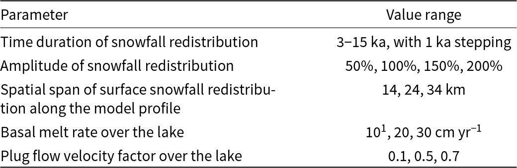
Table 3. Parameters setup for the nine runs with the smallest mismatch RMS values
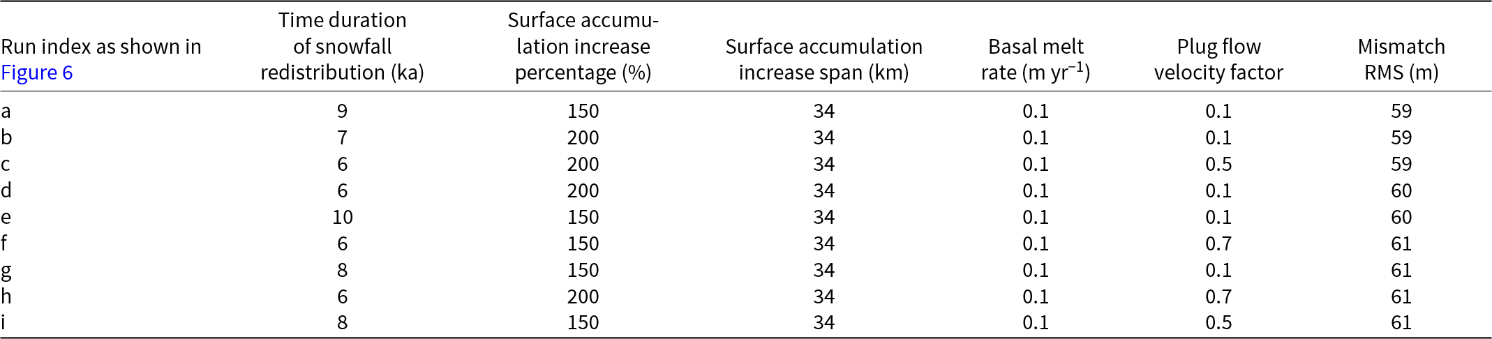
The mismatch contours produced by the model setups listed here are shown in Figure 6.
Within this series of model setups, 21 parameter combinations produce a mismatch RMS value less than the aforementioned 65 m threshold (Figs 6, 7, S7, Tables 3 and S1). As noted, we cannot reliably distinguish these setups as their mismatch falls into the margin of uncertainty. However, these 21 setups collectively represent the best fit achievable with our current understanding. Figure 7 shows the parameter distribution of these 21 setups. The parameter values of the accepted combinations provide valuable constraints on the processes driving the stratigraphic disruption above LSE:
• The snowfall redistribution duration of all 21 accepted setups range between 5 and 11 ka, with no durations falling outside this range yielding a mismatch RMS smaller than the 65-m threshold (Fig. 7a). A snowfall redistribution with a duration within this range produce a thicker ice unit at the upper ice column without significantly changing the shape of the lower IRHs. Because snowfall redistribution is likely to be currently present above LSE, the duration of this process can offer information about its initiation time. Therefore, our result indicates that the snowfall redistribution in the study area only started in the Holocene epoch and was not present prior to this period.
• All accepted setups implement snowfall redistribution amplitudes larger than 150% (Fig. 7b), and the spatial extent of snowfall redistribution in all but one of the accepted setups is 34 km (Fig. 7c), suggesting that a large area of strong snowfall redistribution is needed to produce the observed englacial stratigraphy.
• The modeling result shows all of the combinations implement a low basal melt rate of ∼0.1 m yr−1 (Fig. 7d).
• Lastly, no distinct optimum is observed in the tested plug flow factor values (Fig. 7e). This result indicates that the shift from frozen bed to lubricated bed, and the consequential change in the englacial strain and stress fields, doesn’t have a strong influence on the englacial stratigraphy in the upper ice column, which is expected for an area with low ice-flow velocity.
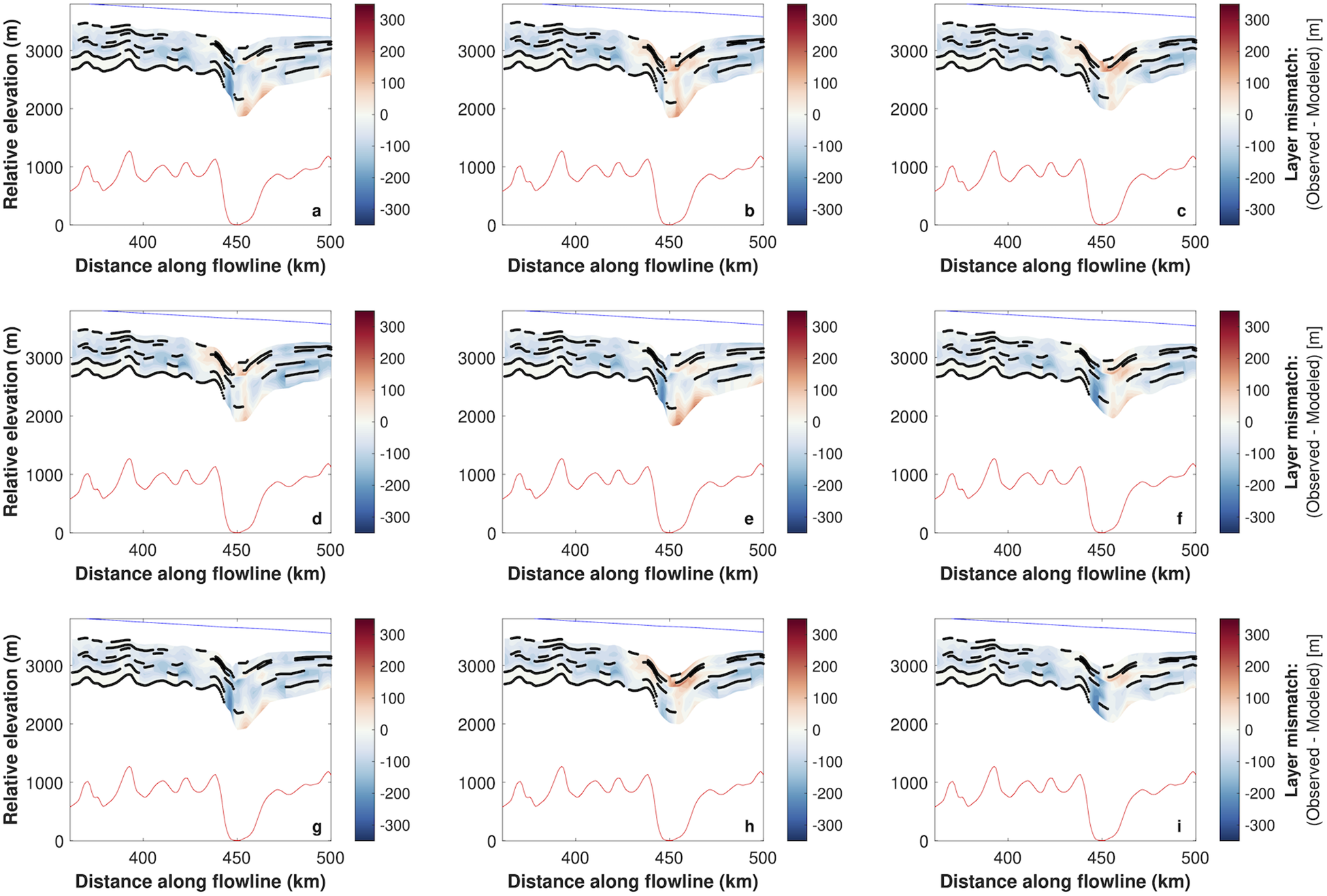
Figure 6. Contour visualization of the 9 model setups that produce the best matches with the observed englacial stratigraphy among the 1404 tested setups. For the purpose of keeping figures concise, we show the nine accepted setups (a-i) with the smallest mismatch RMS here, with their parameters value listed in Table 3. The mismatch from the other 12 accepted setups is shown in Figure S7 in the supplementary material, with their parameter combinations listed in Table S1 in the supplementary material. Blue color means that the observed IRH is deeper than the modeled IRH, and black dots show the modeled IRHs depth where the traced IRHs depth is absent.
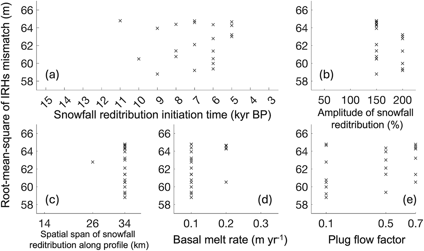
Figure 7. Statistics of the tunable parameter values for the 21 model setups with RMS mismatch less than 65 m, i.e.“accepted setups”. (a) Snowfall redistribution initiation time of the accepted setups. (b) Snowfall redistribution amplitude of the accepted setups. (c) Snowfall redistribution spatial extent of the accepted setups. (d) Basal melting rate of the accepted setups. (e) Plug flow factor of the accepted setups.
4. Discussion
4.1. Holocene evolution of LSE
Our modeling suggests that the irregular englacial stratigraphy observed above LSE cannot be matched as well without a time-variant surface snowfall redistribution (Fig. 7). The surface snowfall redistribution is caused by the local ice surface slope variation above LSE, which is induced by the presence of a major subglacial lake and the resulting basal lubrication. Therefore, a potential driver for such time-variant snowfall redistribution can be subglacial drainage and refilling through time that can alter the water volume of LSE. The LSE bathymetry constrained by Yan (Reference Yan2022) reveals deep basins in the grid northeast part of the lake. This finding suggests that as the lake water volume increases, (i) along the ice-flow direction, the area of basal lubrication would primarily expand upstream, and (ii) across the ice-flow direction, basal lubrication would predominantly extend toward the grid-west direction along the subglacial canyon. When the basal lubrication area reaches a sufficient size, the entire ice column can shift into plug flow, resulting in localized variations in ice surface slope over the lubricated area—this is observed as a localized ∼20 m depression of ice surface elevation over LSE (Figs S8 and S9). This lake activation can lead to the local redistribution of surface snow, with a notable increase in the surface accumulation rate at the surface depression compared to the surrounding areas. This mechanism establishes a connection between the time span of surface accumulation anomaly and that of LSE’s water volume reaching the present level. The modeling results show that the better fits occur when the surface accumulation anomaly begins only around the early Holocene (Fig. 7), which could indicate that LSE experienced a substantial increase of water volume at this time. While we cannot quantify the exact amount of this water volume increase, our modeling results suggest that prior to this era, the water volume was insufficient to generate an area of basal lubrication as widespread as present.
The Holocene increase of LSE water volume inferred in this study is likely a part of a larger scale evolution of the subglacial hydrological system in the interior of East Antarctica. The location and volume of subglacial lakes are determined by both subglacial hydraulic slope and subglacial topographic slope (Dowdeswell and Siegert, Reference Dowdeswell and Siegert1999; Wright and Siegert, Reference Wright, Siegert, Siegert, Kennicutt and Bindschadler2011). Under the contemporary East Antarctic Ice Sheet (EAIS) configuration, the upstream catchment of LSE originates near Ridge B in central East Antarctica. However, since the Last Glacial Maximum, the EAIS has experienced significant changes in ice thickness and volume (e.g. Gowan and others, Reference Gowan2021), which could have induced substantial changes in subglacial hydraulic slope and water routing and resulted in subglacial water being stored in different locations than in the past (Wright and others, Reference Wright, Siegert, Le Brocq and Gore2008). Additionally, the presence of sedimentary basins and groundwater systems in parts of Antarctica (e.g. Gustafson and others, Reference Gustafson2022; Li and others, Reference Li, Aitken, Lindsay and Kulessa2022), along with spatially heterogeneous subglacial thermal conditions (e.g. Shackleton and others, Reference Shackleton, Matsuoka, Moholdt, Van Liefferinge and Paden2023), suggests that changes in water routing could significantly influence the degree of heat exchange that subglacial water experiences as it travels from upstream sources to downstream lake basins. This may alter the basal thermal conditions in downstream areas, potentially impacting the basal melt rate and even the stability of the ice sheet in those regions. The increase of LSE water volume in the Holocene underscores the potential sensitivity of a major Antarctic subglacial lake to the change of glacial and climate conditions.
The hydrological evolution of LSE constrained in this study offers a critical reference for the future interpretation of the sedimentary record preserved at the lake bottom (Yan and others, Reference Yan2022). Specifically, (a) changes in lake water volume and basal melt rate can alter lake circulation patterns, potentially redistributing sediments after their initial deposition (Filina and others, Reference Filina, Blankenship, Thoma, Lukin, Masolov and Sen2008); (b) change of upstream catchment could shift the source and composition of the sediment transported by subglacial water flow; and (c) lake filling could result in ungrounding of sediment, influencing its depositional environment and stability (Smith and others, Reference Smith2018). These factors must be considered and evaluated when selecting the drilling site for lake access and interpreting the LSE sediment record in the future.
Our work opens up the potential for similar approaches to be applied to other large topographically constrained subglacial lakes, enabling investigation of time-dependent volume change of very large subglacial lakes, thought previously to be isolated and stable (Dowdeswell and Siegert, Reference Dowdeswell and Siegert1999; Siegert and others, Reference Siegert2005). Several previous studies have utilized satellite observations to investigate the migration of subglacial water and the draining and filling of subglacial lakes (e.g. Wingham and others, Reference Wingham, Siegert, Shepherd and Muir2006; Carter and others, Reference Carter2011; Fricker and others, Reference Fricker, Siegfried, Carter and Scambos2016), through the observed local-scale changes of ice surface elevation that cannot be attributed to other mechanisms. Such lakes are characterized by being largely unconstrained by basal topography, thus making them susceptible to modest glaciological changes (Siegert and others, Reference Siegert2014). This study differs from previous investigations, as it demonstrates volume change within a subglacial lake constrained well by deep basal topography. Extending from this work, a broader investigation could potentially provide valuable insights into the coupled evolution between Antarctic subglacial hydrology and the Antarctic ice sheet on centennial to millennial timescales, and not just across subglacial lakes.
While it is reasonable to assume that continental-scale ice sheet adjustment might lead to volume loss/gain in large subglacial lakes, this paper provides the first evidence of it. Previously, the morphological signature of colossal volumes of basal water evacuated from the East Antarctic Ice Sheet has been found in the western Dry Valleys; the so-called ‘Labyrinth’ and associated landforms that formed in the Miocene ∼14 Ma (Denton and Sugden, Reference Denton and Sugden2005). Such morphology, involving kilometer-scale channels cut into bedrock, appear far too big to be the result of small ‘active’ lake outburst. Although the presence and location of large Antarctic subglacial lakes at this time may remain challenging to appreciate, the process by which significant water loss may occur from them provides a mechanism that may be relevant to the Labyrinth’s formation.
4.2. Limitation of this study
In this study, the analysis of anomalous englacial stratigraphy above LSE is limited to information from available data, and in particular the lack of 3-D measurements of surface and basal boundary conditions has limited the complexity of the ice-flow model that we can apply. While estimates of these boundary conditions can be inferred from indirect measurements and modeling approaches, the absence of direct, high-resolution measurements, such as in situ measurements of surface accumulation rate, is limiting. In a simple model, the intricate interplay among these boundary conditions can also introduce a trade-off effect, making it challenging to precisely evaluate the impact of each individual parameter choice in isolation. We employ a simplified 2.5D flowband model, because a 3D full-Stokes model, and especially a coupled lake-circulation model, would not be appropriately constrained in this study. A simplified modeling approach is also consistent with our goal, which is to prioritize the identification of first order causes for the observed englacial stratigraphic anomalies above LSE. However, more sophisticated models have been applied to subglacial lakes in problems where englacial stratigraphy is also evaluated. For example, Gudlaugsson et al. (Reference Gudlaugsson, Humbert, Kleiner, Kohler and Andreassen2016) used a 3-D full-Stokes ice-flow model to investigate lake drainage events. There are processes and complexities within the lake, as well as at the transition between grounded and floating ice, that we do not capture in our simplified approach. In particular, our steady state model does not fully reproduce the meters to tens of meters scale observed changes in surface slope and elevation upstream of LSE (Figs S8 and S9), which are likely driven by changes in bed topography and/or basal conditions. This is worth investigating more in the future, especially if 3-D data become available. Future studies, incorporating additional direct measurements, have the potential to conduct a more comprehensive investigation into the dynamics and evolution of the system.
The complex topographic setting of the LSE area imposes challenges for the ice-flow model used in this study (Figs 1b and 4a). The ice-flow model assumes the SIA across the model domain except over the lake when it is active (Cuffey and Paterson, Reference Cuffey and Paterson2010). The simplicity of the model allows us to efficiently conduct a suite of experiments and isolate the influence of a smaller set of key parameter values. However, the model may not adequately account for local variations in the englacial velocity field induced by small-scale subglacial topographic features. LSE is located inside a subglacial canyon channel, whose main axis is oriented orthogonally to the local ice-flow direction. The along-flow topographic relief of the canyon channel exceeds 1000 m over just a few kilometers (Yan and others, Reference Yan2022). Such extreme subglacial topographic relief can complicate the ice flow, and these 3-D effects are not adequately represented in the simple model used in this study. Consequently, the englacial velocity field in the model, particularly in regions closer to the ice–rock interface, may be misrepresented. This likely is the primary source of the persistent negative mismatch above the upstream canyon wall that is observed in all model runs (Figs 5, 6 and S7). To address these limitations, future research can benefit from improved resolution of the subglacial topography, potentially through additional measurements and techniques such as geostatistical realization (e.g. MacKie and others, Reference MacKie, Schroeder, Zuo, Yin and Caers2021). Moreover, incorporating more sophisticated modeling approaches (e.g. Shapero and others, Reference Shapero, Badgeley, Hoffman and Joughin2021)—capable of better representing the strain and stress fields induced by extreme subglacial topographic relief—would enhance the accuracy of future simulations and reduce the observed mismatches.
We expect that the irregular layering in the vicinity of and across LSE has developed locally. Internal layers reflect the influence of surface and basal boundary conditions, both at the location where boundary conditions change and integrated along flow. While internal structure related to changes in boundary conditions can be advected downstream, this structure will become diffused unless spatial and/or temporal changes in boundary conditions persist. In our case, the transition in surface and basal conditions associated with lake initiation is a significant change in boundary conditions. We do not have evidence of upstream changes in boundary conditions that are like this, though they cannot be ruled out. Leysinger Vieli et al. (Reference Leysinger Vieli, Hindmarsh and Siegert2007) provided some intuition about 3-D layer geometries resulting from changes in flow mode, though not specifically for a subglacial lake, which shows the most significant irregularities in layering very near to the location where boundary conditions change. They discussed how layer shape may be affected downstream, but this was to a more muted degree. Our model domain extends from the upstream ice divide, where the ice flow originates, so the upstream influences on layer structure that are included in the model will be reflected in the stratigraphy at LSE.
In this study, we implemented a simplified assumption of homogeneous basal melt rate across the ice–water interface for LSE. In reality, basal melt and freezing rates are likely to vary due to factors such as lake circulation, spatial heterogeneities in geothermal heat flux, and local ice dynamics (e.g. Siegert and others, Reference Siegert2005; Filina and others, Reference Filina, Blankenship, Thoma, Lukin, Masolov and Sen2008). However, due to the current lack of reliable estimates for the lake’s circulation patterns and the surrounding subglacial geological and hydrological conditions, it is difficult to estimate the spatial distribution of basal melting and freezing. Therefore, as an initial step toward understanding the basal melt pattern, we have assumed a homogeneous basal melt rate in this study. Future studies are encouraged to consider spatial variability in basal melting and freezing rates as more measurements and data become available.
We note that the satellite-measured ice-flow velocity in the LSE area are often close to, or even below, the measurement uncertainty (Figs 1 and 4) (Rignot and others, Reference Rignot, Mouginot and Scheuchl2017). This introduces a significant limitation, as small-scale variations in ice-flow speed and direction cannot be reliably resolved. Given the complex subglacial topography of the region, it is likely that such small-scale variations are prevalent. However, due to the inability to fully capture these variations through measurements, they are not well represented in our model. As a result, their potential imprint on englacial stratigraphy cannot be thoroughly investigated. Future in situ measurements of ice-flow velocity in this area will be very valuable for resolving these small-scale variations, allowing for a more accurate representation of their influence on englacial stratigraphy.
5. Conclusion
In this study, we map out the englacial radio-stratigraphy in the LSE area, where we observe a disruption of englacial stratigraphy above the lake, situated over an englacial reflection that is estimated to be ∼12 ka old. We use a 2.5-D ice-flow model to investigate the first order causes for this stratigraphic disruption. After comparing the model output using a suite of runs that evaluated 1404 different parameter combinations, our modeling results indicate changes in the production and transport of water in the wider catchment during the last glacial transition likely led to a significant increase in LSE water level and volume. This inference offers a rare insight into the sensitivity of a major Antarctic subglacial lake to the changes of climate and glacial conditions and underscores the impact that environmental changes can have on subglacial water bodies.
Previous studies have shown that subglacial lake water volumes can fluctuate on yearly-to-decadal time scales (e.g. Livingstone and others, Reference Livingstone2022), where lakes are largely unconstrained by topography and are hence sensitive to relatively small glaciological changes, often dictated by the water volume itself (i.e. self-regulating). No large topographically constrained subglacial lake has previously been shown to have experienced volume change. Our work reveals even large topographically constrained lakes can experience volume change, not over years to decades due to small glaciological adjustments, but likely over centuries and due to major glaciological reconfigurations. This finding opens the possibility of water volume adjustments over glacial cycles to lake environments thought previously to be stable to external influences.
Supplementary material
The supplementary material for this article can be found at https://doi.org/10.1017/jog.2025.15.
Data availability statement
Ice thickness and bed elevation data of Princess Elizabeth Land, East Antarctica used in this study is from Cui (Reference Cui2020), which can be found at https://doi.org/10.5281/zenodo.4023343. The ice surface velocity used in this study is from MEaSUREs InSAR-Based Antarctic Ice Velocity Map, Version 2 (Rignot and others, Reference Rignot, Mouginot and Scheuchl2017), which can be found at https://nsidc.org/data/nsidc-0484/versions/2. The englacial IRH picks done for this study can be found at https://doi.org/10.5281/zenodo.14962526. Original radargrams collected in the study area by ICECAP2 are available upon contacting the authors.
Acknowledgements
We are grateful for the generous financial, logistical, and technical support from: the G. Unger Vetlesen Foundation (New York, USA), University of Texas Institute for Geophysics, the National Science Foundation Center for Oldest Ice Exploration (NSF COLDEX), the Antarctic Gateway Partnership (University of Tasmania, Australia), the University of Washington, the Polar Research Institute of China, the National Natural Science Foundation of China (grant 41876227), the Australian Antarctic Division, and the Global Innovation Initiative jointly funded by the U.S. Department of State and the UK Foreign Office. This work was in part supported by U.S. National Science Foundation grants 1443690 and OPP-2114454. We express our gratitude toward the expeditioners of the Chinese National Antarctic Research Expedition (CHINARE) 33rd and 34th field seasons and the Australian Antarctic Division–University of Texas Institute for Geophysics 4346/ICP10 field campaign. We thank S. Kempf, M. Wiederspahn and G. Ng for their assistance with data processing. We acknowledge support of this work by Landmark Software and Services, a Halliburton Company. We thank Prof. Neil Ross and two anonymous reviewers for reviewing this manuscript and providing valuable feedback that significantly improved the quality of this manuscript. We thank Dr. Dustin Schroeder and Prof. Frank Pattyn for their time and effort in overseeing the review process and editing this manuscript. This is UTIG contribution #4004.
Competing interests
The authors declare no competing interests.


 Open access