


Introduction
In many scenarios, controlling Cyber-Physical Systems (CPS) requires solving planning problems for complex rule-based tasks. Linear temporal logic (LTL) (Pnueli, Reference Pnueli1977) is a symbolic language for specifying such objectives. When a CPS can be modeled by Markov decision processes (MDPs), the planning problems of finding the optimal policy to maximize the probability of achieving an LTL objective can be solved by model-checking techniques (Baier and Katoen, Reference Baier and Katoen2008; Fainekos et al., Reference Fainekos, Kress-Gazit and Pappas2005; Kress-Gazit et al., Reference Kress-Gazit, Fainekos and Pappas2009).
However, LTL planning techniques such as model checking are limited when the transition probabilities of the underlying MDP are unknown. A promising alternative in such cases is reinforcement learning (RL) (Sutton and Barto, Reference Sutton and Barto2018), which finds the optimal policy through sampling. Early efforts in this direction have been confined to particular subsets of LTL (e.g. Cohen and Belta, Reference Cohen, Belta, Cohen and Belta2023; Li and Belta, Reference Li and Belta2019; Li, Vasile et al., Reference Li, Vasile and Belta2017), relied restricted semantics (e.g. Littman et al., Reference Littman, Topcu, Fu, Isbell, Wen and MacGlashan2017), or assumed prior knowledge of the MDP’s topology (e.g. Fu and Topcu, Reference Fu and Topcu2014) – understanding the presence or absence of transitions between any two given states. Model-based RL methods have also been applied by first estimating all the transitions of the MDP and applying model checking with a consideration on the estimation error (Brázdil et al., Reference Brázdil, Chatterjee, Chmelík, Forejt, Křetínský, Kwiatkowska, Parker, Ujma, Cassez and Raskin2014). However, the computation complexity can be unnecessarily high since not all transitions are equally relevant (Ashok et al., Reference Ashok, Křetínský, Weininger, Dillig and Tasiran2019).
Recent works have used model-free RL for LTL objectives on MDPs with unknown transition probabilities (Bozkurt et al., Reference Bozkurt, Wang, Zavlanos and Pajic2020; Hahn et al., Reference Hahn, Perez, Schewe, Somenzi, Trivedi and Wojtczak2020; M Hasanbeig et al., Reference Hasanbeig, Kantaros, Abate, Kroening, Pappas and Lee2019; Sadigh et al., Reference Sadigh, Kim, Coogan, Sastry and Seshia2014). These approaches are all based on constructing
 $\omega$
-regular automata for the LTL objectives and translating the LTL objective into surrogate rewards within the product of the MDP and the automaton. The surrogate rewards yield the Bellman equations for the satisfaction probability of the LTL objective for a given policy, which can be solved via RL through sampling.
$\omega$
-regular automata for the LTL objectives and translating the LTL objective into surrogate rewards within the product of the MDP and the automaton. The surrogate rewards yield the Bellman equations for the satisfaction probability of the LTL objective for a given policy, which can be solved via RL through sampling.
The first approach (Sadigh et al., Reference Sadigh, Kim, Coogan, Sastry and Seshia2014) employs Rabin automata to transform LTL objectives into Rabin objectives, which are then translated into surrogate rewards, assigning constant positive rewards to certain “good” states and negative rewards to “bad” states. However, this surrogate reward function is not technically correct, as demonstrated in (Hahn et al., Reference Hahn, Perez, Schewe, Somenzi, Trivedi, Wojtczak, Vojnar and Zhang2019). The second approach (M Hasanbeig et al., Reference Hasanbeig, Kantaros, Abate, Kroening, Pappas and Lee2019) employs limit-deterministic Büchi automata to translate LTL objectives into surrogate rewards that assign a constant reward for “good” states with a constant discount factor. This approach is also technically flawed, as demonstrated by (Hahn et al., Reference Hahn, Perez, Schewe, Somenzi, Trivedi and Wojtczak2020). The third method (Bozkurt et al., Reference Bozkurt, Wang, Zavlanos and Pajic2020) also utilizes limit-deterministic Büchi automata but introduces surrogate rewards featuring a constant reward for “good” states and two discount factors that are constants but very close to 1.
In more recent works (Cai, M Hasanbeig et al., Reference Cai, Hasanbeig, Xiao, Abate and Kan2021; H Hasanbeig et al., Reference Hasanbeig, Kroening and Abate2023; Shao and Kwiatkowska, Reference Shao and Kwiatkowska2023; Voloshin et al., Reference Voloshin, Verma and Yue2023), the surrogate reward with two discount factors from (Bozkurt et al., Reference Bozkurt, Wang, Zavlanos and Pajic2020) was used while allowing one discount factor to be equal to 1. We noticed that in this case, the Bellman equation may have multiple solutions, as that discount factor of 1 does not provide contraction in many states for the Bellman operator. Consequently, the RL algorithm may fail to converge or may converge to a solution that deviates from the satisfaction probabilities of the LTL objective, resulting in suboptimal policies. To illustrate this, we present a concrete example. To correctly identify the satisfaction probabilities from the multiple solutions, we propose a sufficient condition that ensures uniqueness: the solution of the Bellman equation must be 0 for all states within rejecting bottom strongly connected components (BSCCs).
We prove that, under this sufficient condition, the Bellman equation has a unique solution that approximates the satisfaction probabilities of LTL objectives by the following procedure. When one of the discount factors equals 1, we partition the state space into states with discounting and states without discounting based on surrogate reward. In this case, We first establish the relationships among all states with discounting and show that their solution is unique since the Bellman operator remains contractive in these states. Then, we show that the entire solution is unique since the solution on states without discounting is uniquely determined by states with discounting.
Finally, we present a case study demonstrating that correctly solving the Bellman equation requires the uniqueness condition. We further show that when neural networks are used to approximate the Bellman equation’s solution, as is common in deep RL for LTL objectives, this condition is automatically violated.
Related works
We study a special form of the Bellman equation encoutered in LTL planning problem that may admit multiple solutions. In contrast, prior works have primarily analyzed the accuracy of solving a Bellman equation with a unique solution. The relationship between the accuracy of solving the Bellman equation with respect to the Bellman equation residuals has been discussed by many works (Bertsekas, Reference Bertsekas, Floudas and Pardalos2001; Heger, Reference Heger1996; Munos, Reference Munos2003, Reference Munos2007; Singh and Yee, Reference Singh and Yee1994). Later work exposes several limits when solving Bellman equation via samples. Off-policy training can be unstable and depends on the sampling distribution (Geist et al., Reference Geist, Piot and Pietquin2017; Kolter, Reference Kolter, Shawe-Taylor, Zemel, Bartlett, Pereira and Weinberger2011). Under aliasing, the Bellman residual may be unlearnable (Sutton and Barto, Reference Sutton and Barto2018). In offline RL, Bellman error has weak correspondence to value accuracy and control performance (Fujimoto et al., Reference Fujimoto, Meger, Precup, Nachum and Gu2022). These results assume a unique fixed point. In contrast, we show that in the LTL surrogate reward setting the Bellman equation can be non-contractive on parts of the state space, so Bellman equation may have multiple solutions.
Part of the theoretical results have appeared in our previous paper (Xuan, Bozkurt et al., Reference Xuan, Bozkurt, Pajic and Wang2024) without proofs and demonstration on case studies.
Preliminaries
This section introduces preliminaries on labeled Markov decision processes, linear temporal logic, and probabilistic model checking.
Labeled Markov decision processes
Labeled Markov decision processes (LMDPs) are used to model planning problems where each decision has a potentially probabilistic outcome. LMDPs augment standard Markov decision processes (Baier and Katoen, Reference Baier and Katoen2008) with state labels, allowing properties such as safety and liveness to be assigned to a sequences of states.
Definition 1. A labeled Markov decision process is a tuple
 ${\mathcal{M}} = (S, A, P, s_{\rm init}, \Lambda, L)$
where
${\mathcal{M}} = (S, A, P, s_{\rm init}, \Lambda, L)$
where
-
S is a finite set of states and
 $s_{\rm init}\,\in\, S$
is the initial state,
$s_{\rm init}\,\in\, S$
is the initial state,
-
A is a finite set of actions where A(s) denotes the set of allowed actions in state
$s\in S$
, -
$P: S \times A \times S \to [0,1]$
is the transition probability function such that for all
$s\in S$
,
$$ \sum\limits_{s' \in S} P (s,a,s') = \left\{ {\matrix{ {1,} \hfill & {a \in A(s)} \hfill \cr {0,} \hfill & {a \; \notin \; A(s)} \hfill \cr } } \right.,$$
-
$\Lambda$
is a finite set of atomic propositions,
-
$L: S \to 2^{\Lambda}$
is a labeling function.


A path of the LMDP
 ${\mathcal{M}}$
is an infinite state sequence
${\mathcal{M}}$
is an infinite state sequence
 ${\unicode{x03C3}} = s_0 s_1 s_2 \cdots$
such that for all
${\unicode{x03C3}} = s_0 s_1 s_2 \cdots$
such that for all
 $i \ge 0$
, there exists
$i \ge 0$
, there exists
 $a_i\,\in\, A(s)$
and
$a_i\,\in\, A(s)$
and
 $s_{i}, s_{i+1}\,\in\, S$
with
$s_{i}, s_{i+1}\,\in\, S$
with
 $P(s_i,a_i,s_{i+1}) \gt 0$
. The semantic path corresponding to
$P(s_i,a_i,s_{i+1}) \gt 0$
. The semantic path corresponding to
 ${\unicode{x03C3}}$
is given by
${\unicode{x03C3}}$
is given by
 $L({\unicode{x03C3}}) = L(s_0)L( s_1)\cdots$
, derived using the labeling function L(s). Given a path
$L({\unicode{x03C3}}) = L(s_0)L( s_1)\cdots$
, derived using the labeling function L(s). Given a path
 ${\unicode{x03C3}}$
, the ith state is denoted by
${\unicode{x03C3}}$
, the ith state is denoted by
 ${\unicode{x03C3}}[i] = s_i$
. We denote the prefix by
${\unicode{x03C3}}[i] = s_i$
. We denote the prefix by
 ${\unicode{x03C3}}[{:}i] = s_0 s_1\cdots s_i$
and suffix by
${\unicode{x03C3}}[{:}i] = s_0 s_1\cdots s_i$
and suffix by
 ${\unicode{x03C3}}[i{+}1{:}] = s_{i+1} s_{i+2}\cdots$
.
${\unicode{x03C3}}[i{+}1{:}] = s_{i+1} s_{i+2}\cdots$
.
LTL and limit-deterministic Büchi automata
In an LMDP
 ${\mathcal{M}}$
, whether a given semantic path
${\mathcal{M}}$
, whether a given semantic path
 $L({\unicode{x03C3}})$
satisfies a property such as avoiding unsafe states can be expressed using LTL. LTL can specify the change of labels along the path by connecting Boolean variables over the labels with two propositional operators, negation
$L({\unicode{x03C3}})$
satisfies a property such as avoiding unsafe states can be expressed using LTL. LTL can specify the change of labels along the path by connecting Boolean variables over the labels with two propositional operators, negation
 $(\neg)$
and conjunction
$(\neg)$
and conjunction
 $(\wedge)$
, and two temporal operators, next
$(\wedge)$
, and two temporal operators, next
 $(\bigcirc)$
and until
$(\bigcirc)$
and until
 $(\cup)$
.
$(\cup)$
.
Definition 2. The LTL formula is defined by the syntax
 $${\unicode{x03C6}} :: = {\rm{true}}\,\left| \alpha \right|\,{{\unicode{x03C6}} _1} \wedge {{\unicode{x03C6}} _2}\,|\neg {\unicode{x03C6}} | \bigcirc {\unicode{x03C6}} \,|\,{{\unicode{x03C6}} _1} \cup {{\unicode{x03C6}} _2},\alpha\,\in\, \Lambda.$$
Satisfaction of an LTL formula
 ${\unicode{x03C6}}$
on a path
${\unicode{x03C6}}$
on a path
 ${\unicode{x03C3}}$
of an MDP (denoted by
${\unicode{x03C3}}$
of an MDP (denoted by
 ${\unicode{x03C3}} \models {\unicode{x03C6}}$
) is defined as,
${\unicode{x03C3}} \models {\unicode{x03C6}}$
) is defined as,
 $\alpha\in \Lambda$
is satisfied on
$\alpha\in \Lambda$
is satisfied on
 ${\unicode{x03C3}}$
if
${\unicode{x03C3}}$
if
 $\alpha\in L({\unicode{x03C3}}[1])$
,
$\alpha\in L({\unicode{x03C3}}[1])$
,
 $\bigcirc {\unicode{x03C6}}$
is satisfied on
$\bigcirc {\unicode{x03C6}}$
is satisfied on
 ${\unicode{x03C3}}$
if
${\unicode{x03C3}}$
if
 ${\unicode{x03C6}}$
is satisfied on
${\unicode{x03C6}}$
is satisfied on
 ${\unicode{x03C3}}[1{:}]$
,
${\unicode{x03C3}}[1{:}]$
,
 ${\unicode{x03C6}}_1 \cup {\unicode{x03C6}}_2$
is satisfied on
${\unicode{x03C6}}_1 \cup {\unicode{x03C6}}_2$
is satisfied on
 ${\unicode{x03C3}}$
if there exists i such that
${\unicode{x03C3}}$
if there exists i such that
 ${\unicode{x03C3}}[i{:}] \models {\unicode{x03C6}}_2$
and for all
${\unicode{x03C3}}[i{:}] \models {\unicode{x03C6}}_2$
and for all
 $j \lt i,{\mkern 1mu} {\unicode{x03C3}} [j:] \models {{\unicode{x03C6}} _1}$
.
$j \lt i,{\mkern 1mu} {\unicode{x03C3}} [j:] \models {{\unicode{x03C6}} _1}$
.
Other propositional and temporal operators can be derived from previous operators, e.g., (or)
 ${\unicode{x03C6}}_1 \vee {\unicode{x03C6}}_2 := \neg(\neg {\unicode{x03C6}}_1 \wedge \neg {\unicode{x03C6}}_2)$
, (eventually)
${\unicode{x03C6}}_1 \vee {\unicode{x03C6}}_2 := \neg(\neg {\unicode{x03C6}}_1 \wedge \neg {\unicode{x03C6}}_2)$
, (eventually)
 $\lozenge {\unicode{x03C6}} := {\rm true} \cup {\unicode{x03C6}}$
and (always)
$\lozenge {\unicode{x03C6}} := {\rm true} \cup {\unicode{x03C6}}$
and (always)
 $ \square {\unicode{x03C6}} := \neg \lozenge \neg {\unicode{x03C6}}$
.
$ \square {\unicode{x03C6}} := \neg \lozenge \neg {\unicode{x03C6}}$
.
We can use Limit-Deterministic Büchi Automata (LDBA) to check the satisfaction of an LTL formula on a path.
Definition 3. An LDBA is a tuple
 $\mathcal{A} = ({\mathcal Q},\Sigma,{\rm\delta},{\rm q_0},B)$
where
$\mathcal{A} = ({\mathcal Q},\Sigma,{\rm\delta},{\rm q_0},B)$
where
 $\mathcal{Q}$
is a finite set of automaton states,
$\mathcal{Q}$
is a finite set of automaton states,
 $\Sigma$
is a finite alphabet,
$\Sigma$
is a finite alphabet,
 ${\rm\delta}:{\mathcal Q}\times (\Sigma \cup \{\epsilon\})\to {2}^{\mathcal{Q}}$
is a (partial) transition function,
${\rm\delta}:{\mathcal Q}\times (\Sigma \cup \{\epsilon\})\to {2}^{\mathcal{Q}}$
is a (partial) transition function,
 $q_0$
is an initial state, and B is a set of accepting states,
$q_0$
is an initial state, and B is a set of accepting states,
 ${\rm\delta}$
is total except for the
${\rm\delta}$
is total except for the
 $\epsilon$
-transitions (
$\epsilon$
-transitions (
 $|{\rm\delta}(q,\alpha)|=1$
for all
$|{\rm\delta}(q,\alpha)|=1$
for all
 $q\in {\mathcal{Q}}, \alpha\,\in\, \Sigma$
), and there exists a bipartition of
$q\in {\mathcal{Q}}, \alpha\,\in\, \Sigma$
), and there exists a bipartition of
 $\mathcal{Q}$
to an initial and an accepting component
$\mathcal{Q}$
to an initial and an accepting component
 ${\mathcal{Q}}_{{ini}}\cup {\mathcal{Q}}_{\it{acc}} = {\mathcal{Q}}$
such that
${\mathcal{Q}}_{{ini}}\cup {\mathcal{Q}}_{\it{acc}} = {\mathcal{Q}}$
such that
-
there is no transition from
$\mathcal{Q}_{\it{acc}}$
to
$\mathcal{Q}_{\it{ini}}$
, i.e., for any
$q\in {\mathcal{Q}}_{\it{acc}}, v\in \Sigma, {\rm\delta}( q,v)\subseteq {\mathcal{Q}}_{\it{acc}}$
, -
all the accepting states are in
$\mathcal{Q}_{\it{acc}}$
, i.e.,
$B\subseteq {\mathcal{Q}}_{\it{acc}}$
, -
$\mathcal{Q}_{\it{acc}}$
does not have any outgoing
$\epsilon$
-transitions, i.e.,
${\rm\delta}(q,\epsilon)=\emptyset$
for any
$q\in {\mathcal{Q}}_{\it{acc}}$
.


A run is an infinite sequence of transitions
 ${\unicode{x03C1}} = (q_0,w_0,q_1), (q_1,w_1, q_2) \cdots$
such that for all
${\unicode{x03C1}} = (q_0,w_0,q_1), (q_1,w_1, q_2) \cdots$
such that for all
 $i \ge 0$
,
$i \ge 0$
,
 $q_{i+1}\,\in\, {\rm\delta}(q_i, w_i)$
. The run
$q_{i+1}\,\in\, {\rm\delta}(q_i, w_i)$
. The run
 ${\unicode{x03C1}}$
is accepted by the LDBA if it satisfies the Büchi condition, i.e.,
${\unicode{x03C1}}$
is accepted by the LDBA if it satisfies the Büchi condition, i.e.,
 ${\rm inf}(\rm {\unicode{x03C1}}) \cap B \ne \emptyset$
, where
${\rm inf}(\rm {\unicode{x03C1}}) \cap B \ne \emptyset$
, where
 ${\rm inf}(\rm {\unicode{x03C1}})$
denotes the set of automaton states visited by
${\rm inf}(\rm {\unicode{x03C1}})$
denotes the set of automaton states visited by
 ${\unicode{x03C1}}$
infinitely many times.
${\unicode{x03C1}}$
infinitely many times.
A path
 ${\unicode{x03C3}}=s_0s_1\dots$
of an LMDP
${\unicode{x03C3}}=s_0s_1\dots$
of an LMDP
 ${\mathcal{M}}$
is considered accepted by an LDBA
${\mathcal{M}}$
is considered accepted by an LDBA
 $\mathcal{A}$
if the semantic path
$\mathcal{A}$
if the semantic path
 $L({\unicode{x03C3}})$
is the corresponding word w of an accepting run
$L({\unicode{x03C3}})$
is the corresponding word w of an accepting run
 ${\unicode{x03C1}}$
after elimination of
${\unicode{x03C1}}$
after elimination of
 $\epsilon$
-transitions.
$\epsilon$
-transitions.
Lemma 1. (Sickert et al., Reference Sickert, Esparza, Jaax and Křetínský2016, Theorem 1
) Given an LTL objective
 ${\varphi}$
, there exists an LDBA
${\varphi}$
, there exists an LDBA
 $\mathcal{A}_{\unicode{x03C6}}$
(with labels
$\mathcal{A}_{\unicode{x03C6}}$
(with labels
 $\Sigma=2^{\Lambda}$
) such that a path
$\Sigma=2^{\Lambda}$
) such that a path
 ${\sigma} \models {\varphi}$
if and only if
${\sigma} \models {\varphi}$
if and only if
 ${\sigma}$
is accepted by the LDBA
${\sigma}$
is accepted by the LDBA
 $\mathcal{A}_{\unicode{x03C6}}$
.
$\mathcal{A}_{\unicode{x03C6}}$
.
Product MDP
Planning problems for LTL objectives typically requires a (history-dependent) policy, which determines the current action based on all previous state visits.
Definition 4. A policy
 $\pi$
is a function
$\pi$
is a function
 $\pi:S^+ \to {A}$
such that
$\pi:S^+ \to {A}$
such that
 $\pi({\sigma}[{:}n])\in {A}({\sigma}[n])$
, where
$\pi({\sigma}[{:}n])\in {A}({\sigma}[n])$
, where
 $S^+$
stands for the set all non-empty finite sequences taken from S. A memoryless policy is a policy that only depends on the current state
$S^+$
stands for the set all non-empty finite sequences taken from S. A memoryless policy is a policy that only depends on the current state
 $\pi:S \to {A}$
. Given a LMDP
$\pi:S \to {A}$
. Given a LMDP
 ${\mathcal{M}} = ({ \mathcal{S, A, P}}, s_{\rm 0}, \Lambda, {\mathcal{L}})$
and a memoryless policy
${\mathcal{M}} = ({ \mathcal{S, A, P}}, s_{\rm 0}, \Lambda, {\mathcal{L}})$
and a memoryless policy
 $\pi$
, the Markov chain (MC) induced by policy
$\pi$
, the Markov chain (MC) induced by policy
 $\pi$
is a tuple
$\pi$
is a tuple
 ${\mathcal{M}}_\pi=(S, P_\pi,s_{\rm 0},\Lambda,L)$
where
${\mathcal{M}}_\pi=(S, P_\pi,s_{\rm 0},\Lambda,L)$
where
 $P_\pi(s,s')=P(s,\pi(s),s')$
for all
$P_\pi(s,s')=P(s,\pi(s),s')$
for all
 $s,s'\in S$
.
$s,s'\in S$
.
Using the LDBA, we construct a product MDP that augments the MDP state space along with the automaton state space. The state of the product MDP encodes both the physical state and the progression of the LTL objective. In this manner, we “lift” the planning problem to the product MDP. Given that the state of the product MDP now encodes all the information necessary for planning, the action can be determined by the current state of the product MDP, resulting in memoryless policies. Formally, the product MDP is defined as follows:
Definition 5. A product MDP
 $ {\mathcal{M}}^{\times} = ( S^{\times}, A^{\times}, P^{\times},{\it s}_{\rm 0}^{\times}, B^{\times})$
of an LMDP
$ {\mathcal{M}}^{\times} = ( S^{\times}, A^{\times}, P^{\times},{\it s}_{\rm 0}^{\times}, B^{\times})$
of an LMDP
 $ {\mathcal{M}} = ( S, A, P, {\it s}_{\rm 0}, \Lambda, L)$
and an LDBA
$ {\mathcal{M}} = ( S, A, P, {\it s}_{\rm 0}, \Lambda, L)$
and an LDBA
 ${\mathcal{A}}= (\mathcal{Q}, \Sigma,{\rm\delta},{\it q}_{\rm 0},B)$
is defined by the set of states
${\mathcal{A}}= (\mathcal{Q}, \Sigma,{\rm\delta},{\it q}_{\rm 0},B)$
is defined by the set of states
 $S^\times = S \times {\mathcal{Q}}$
, the set of actions
$S^\times = S \times {\mathcal{Q}}$
, the set of actions
 ${A}^\times = { {A}} \cup \{\epsilon_q|q\in {\mathcal{Q}}\}$
, the transition probability function
${A}^\times = { {A}} \cup \{\epsilon_q|q\in {\mathcal{Q}}\}$
, the transition probability function
 $${P^ \times }(\langle s,q\rangle, a,\langle s',q'\rangle ) = \left\{ {\matrix{ {P(s,a,s')} \hfill & \!\! {q' = {\rm\delta} (q,L(s)),a \,\notin\, {A^{\rm\epsilon}}} \hfill \cr 1 \hfill & {a = {{\rm\epsilon}_{q'}},q'\,\in\, {\rm\delta} (q,),s = s'} \hfill \cr 0 \hfill & {{\rm{otherwise}}} \hfill \cr } } \right.,$$
the initial state
 $s_0^\times=\langle s_0,q_0 \rangle$
, and the set of accepting states
$s_0^\times=\langle s_0,q_0 \rangle$
, and the set of accepting states
 $B^\times=\{\langle s,q \rangle\,\in\, S^\times |q\in B\}$
. We say a path
$B^\times=\{\langle s,q \rangle\,\in\, S^\times |q\in B\}$
. We say a path
 ${\unicode{x03C3}}$
satisfies the Büchi condition
${\unicode{x03C3}}$
satisfies the Büchi condition
 ${\unicode{x03C6}}_B$
if
${\unicode{x03C6}}_B$
if
 ${\rm inf}({\unicode{x03C3}})\cap B^\times\ne\emptyset$
. Here,
${\rm inf}({\unicode{x03C3}})\cap B^\times\ne\emptyset$
. Here,
 ${\rm inf}({\unicode{x03C3}})$
denotes the set of states visited infinitely many times on
${\rm inf}({\unicode{x03C3}})$
denotes the set of states visited infinitely many times on
 ${\unicode{x03C3}}$
.
${\unicode{x03C3}}$
.
The transitions of the product MDP
 ${\mathcal{M}}^\times $
are derived by combining the transitions of the MDP
${\mathcal{M}}^\times $
are derived by combining the transitions of the MDP
 $ {\mathcal{M}} $
and the LDBA
$ {\mathcal{M}} $
and the LDBA
 $ \mathcal{A} $
. Specifically, the multiple
$ \mathcal{A} $
. Specifically, the multiple
 $ \epsilon $
-transitions starting from the same states in the LDBA are differentiated by their respective end states q and are denoted as
$ \epsilon $
-transitions starting from the same states in the LDBA are differentiated by their respective end states q and are denoted as
 $ \epsilon_q$
. These
$ \epsilon_q$
. These
 $ \epsilon $
-transitions in the LDBA give rise to corresponding
$ \epsilon $
-transitions in the LDBA give rise to corresponding
 $ \epsilon $
-actions in the product MDP, each occurring with a probability of 1. The limit-deterministic nature of LDBAs ensures that the presence of these
$ \epsilon $
-actions in the product MDP, each occurring with a probability of 1. The limit-deterministic nature of LDBAs ensures that the presence of these
 $\epsilon$
-actions within the product MDPs does not prevent the quantitative analysis of the MDPs for planning. In other words, any optimal policy for a product MDP induces an optimal policy for the original MDP, as formally stated below.
$\epsilon$
-actions within the product MDPs does not prevent the quantitative analysis of the MDPs for planning. In other words, any optimal policy for a product MDP induces an optimal policy for the original MDP, as formally stated below.
Lemma 2. (Sickert et al., Reference Sickert, Esparza, Jaax and Křetínský2016). Given an LMDP
 ${\mathcal{M}}$
and an LTL objective
${\mathcal{M}}$
and an LTL objective
 ${\unicode{x03C6}}$
, let
${\unicode{x03C6}}$
, let
 $\mathcal{A}_{\unicode{x03C6}}$
be the LDBA derived from
$\mathcal{A}_{\unicode{x03C6}}$
be the LDBA derived from
 ${\unicode{x03C6}}$
and let
${\unicode{x03C6}}$
and let
 ${\mathcal{M}}^\times$
be the product MDP constructed from
${\mathcal{M}}^\times$
be the product MDP constructed from
 ${\mathcal{M}}$
and
${\mathcal{M}}$
and
 $\mathcal{A}_{\unicode{x03C6}}$
, with the set of accepting states
$\mathcal{A}_{\unicode{x03C6}}$
, with the set of accepting states
 $B^\times$
. Then, a memoryless policy
$B^\times$
. Then, a memoryless policy
 $\pi^\times$
that maximizes the probability of satisfying the Büchi condition on
$\pi^\times$
that maximizes the probability of satisfying the Büchi condition on
 ${\mathcal{M}}^\times$
,
${\mathcal{M}}^\times$
,
 $P_{{\unicode{x03C3}}^\times} \big({\unicode{x03C3}}^\times \models \square \lozenge B^\times \big)$
where
$P_{{\unicode{x03C3}}^\times} \big({\unicode{x03C3}}^\times \models \square \lozenge B^\times \big)$
where
 ${\unicode{x03C3}}^\times {\sim} \mathcal{M}_{\pi^\times}^\times$
, induces a finite-memory policy
${\unicode{x03C3}}^\times {\sim} \mathcal{M}_{\pi^\times}^\times$
, induces a finite-memory policy
 $\pi$
that maximizes the satisfaction probability
$\pi$
that maximizes the satisfaction probability
 $P_{{\unicode{x03C3}} \sim \mathcal{M}_{\pi}} \big({\unicode{x03C3}} \models {\unicode{x03C6}} \big)$
on
$P_{{\unicode{x03C3}} \sim \mathcal{M}_{\pi}} \big({\unicode{x03C3}} \models {\unicode{x03C6}} \big)$
on
 ${\mathcal{M}}$
.
${\mathcal{M}}$
.
Problem formulation
In the previous section, we have shown LTL objectives on an LMDP can be converted into a Büchi condition on the Product MDP. In this section, we focus on a surrogate reward commonly used for Büchi condition proposed in (Bozkurt et al., Reference Bozkurt, Wang, Zavlanos and Pajic2020) and study the uniqueness of solution for the Bellman equation of this surrogate reward, which has not been sufficiently discussed in previous work (H Hasanbeig et al., Reference Hasanbeig, Kroening and Abate2023; Shao and Kwiatkowska, Reference Shao and Kwiatkowska2023; Voloshin et al., Reference Voloshin, Verma and Yue2023).
For simplicity, we drop
 $\times$
from the product MDP notation and define the satisfaction probability for the Büchi condition as
$\times$
from the product MDP notation and define the satisfaction probability for the Büchi condition as
 $$P(s \models \square\lozenge B): = {P_{{\unicode{x03C3}} \sim {{\cal M}_\pi }}}({\unicode{x03C3}} \models \square\lozenge B\mid \exists t:{\unicode{x03C3}} [t] = s).$$
When the product MDP model is unknown, the traditional model-based method through graph search (Baier and Katoen, Reference Baier and Katoen2008) is not applicable. Alternatively, we may use model-free RL with a two-discount-factor surrogate reward proposed by (Bozkurt et al., Reference Bozkurt, Wang, Zavlanos and Pajic2020), which has been widely adopted in (Cai, M Hasanbeig et al., Reference Cai, Hasanbeig, Xiao, Abate and Kan2021; Cai, Xiao et al., Reference Cai, Xiao, Li and Kan2023; H Hasanbeig et al., Reference Hasanbeig, Kroening and Abate2023; Shao and Kwiatkowska, Reference Shao and Kwiatkowska2023; Voloshin et al., Reference Voloshin, Verma and Yue2023). This approach involves a reward function
 $R: S\to\mathbb{R}$
and a state-dependent discount factor function
$R: S\to\mathbb{R}$
and a state-dependent discount factor function
 $\Gamma: S\to (0,1]$
with
$\Gamma: S\to (0,1]$
with
 $0 \lt {{\rm\gamma} _B} \lt {\rm\gamma} \le 1$
,
$0 \lt {{\rm\gamma} _B} \lt {\rm\gamma} \le 1$
,
 $$R(s): = \left\{ {\matrix{ {1 - {{\rm\gamma} _B}} \hfill & {s\,\in\, B} \hfill \cr 0 \hfill & {s \,\notin\, B} \hfill \cr } } \right.,\quad \Gamma (s): = \left\{ {\matrix{ {{{\rm\gamma} _B}} \hfill & {s\,\in\, B} \hfill \cr {\rm\gamma} \hfill & {s \,\notin\, B} \hfill \cr } } \right..$$
A positive reward is collected only when an accepting state is visited along the path. The K-step return (
 $K\in \mathbb{N}$
or
$K\in \mathbb{N}$
or
 $K=\infty$
) of a path from time
$K=\infty$
) of a path from time
 $t\in \mathbb{N}$
is
$t\in \mathbb{N}$
is
 $$\matrix{ \hfill {{G_{t:K}}({\unicode{x03C3}} )}\hskip-6pt & { = \sum\limits_{i = 0}^K R ({\unicode{x03C3}} [t + i]) \cdot \prod\limits_{j = 0}^{i - 1} \Gamma ({\unicode{x03C3}} [t + j]),} \hfill \cr \hfill {{G_t}({\unicode{x03C3}} )} \hskip-6pt & { = \mathop {\lim }\limits_{K \to \infty } {G_{t:K}}({\unicode{x03C3}} ).} \hfill \cr } $$
The definition is similar to standard discounted rewards (Sutton and Barto, Reference Sutton and Barto2018) but involves state-dependent discounting factors. If
 ${\rm\gamma}=1$
, then for a path that satisfies the Büchi objective, the return is the summation of a geometric series
${\rm\gamma}=1$
, then for a path that satisfies the Büchi objective, the return is the summation of a geometric series
 $\sum\nolimits_{i = 0}^\infty {(1 - {{\rm\gamma} _B})} {\rm\gamma} _B^i = {{1 - {{\rm\gamma} _B}} \over {1 - {{\rm\gamma} _B}}} = 1$
.
$\sum\nolimits_{i = 0}^\infty {(1 - {{\rm\gamma} _B})} {\rm\gamma} _B^i = {{1 - {{\rm\gamma} _B}} \over {1 - {{\rm\gamma} _B}}} = 1$
.
Accordingly, the value function
 $V_\pi(s)$
is the expected return conditional on the path starting at s under the policy
$V_\pi(s)$
is the expected return conditional on the path starting at s under the policy
 $\pi$
.
$\pi$
.
 $$\matrix{ {{V_\pi }(s)} \hfill & \!\!\!\!{ = {{\mathbb E}_\pi }[{G_t}({\unicode{x03C3}} )|{\unicode{x03C3}} [t] = s]} \hfill \cr {} \hfill & \!\!\!\!{ = {{\mathbb E}_\pi }[{G_t}({\unicode{x03C3}} )\mid {\unicode{x03C3}} [t] = s,{\unicode{x03C3}} \models {\rm{\square}}\lozenge B] \cdot P(s \models {\rm{\square}}\lozenge B)} \hfill \cr {} \hfill & \!\!\!\! { + \,\, {{\mathbb E}_\pi }[{G_t}({\unicode{x03C3}} )\mid {\unicode{x03C3}} [t] = s,{\unicode{x03C3}} \mid\!=\!\!\!\!\!\!\!/\,\,\, {\rm{\square}}\lozenge B] \cdot P(s \mid\!=\!\!\!\!\!\!\!/\,\,\, {\rm{\square}}\lozenge B),} \hfill \cr } $$
where
 $P(s \not\models \square \lozenge B)$
stands for the probability of a path not satisfying the Büchi objective conditional on the path starting at s.
$P(s \not\models \square \lozenge B)$
stands for the probability of a path not satisfying the Büchi objective conditional on the path starting at s.
The value function approximates the satisfaction probability defined in (2) to guide the search for policy. As the value
 ${\rm\gamma}_B$
,
${\rm\gamma}_B$
,
 ${\rm\gamma}$
becomes close to 1, the value function becomes close to
${\rm\gamma}$
becomes close to 1, the value function becomes close to
 $P(s\models \square \lozenge B)$
as
$P(s\models \square \lozenge B)$
as
 $$\eqalign{ & \mathop {\lim }\limits_{{\rm\gamma} \to {1^ - }} {{\mathbb E}_\pi }[{G_t}({\unicode{x03C3}} )\mid {\unicode{x03C3}} [t] = s,{\unicode{x03C3}} \models {\rm{\square}}\lozenge B] = 1 \cr & \mathop {\lim }\limits_{{{\rm\gamma} _B} \to {1^ - }} {{\mathbb E}_\pi }[{G_t}({\unicode{x03C3}} )\mid {\unicode{x03C3}} [t] = s,{\unicode{x03C3}} \not\models {\rm{\square}}\lozenge B] = 0. \cr} $$
Given a policy, the value function satisfies the Bellman equation.Footnote 1 The Bellman equation is derived from the fact that the value of the current state is equal to the expectation of the current reward plus the discounted value of the next state. For the surrogate reward in the equation (3), the Bellman equation is given as follows:
 $$\matrix{ {{V_\pi }(s)} \hfill & {\!\!\!\!\! = \left\{ {\matrix{ {1 - {{\rm\gamma} _B} + {{\rm\gamma} _B}\sum\nolimits_{s'\,\in\, S} {{P_\pi }(s,s'){V_\pi }(s')} } \hfill & {s\,\in\, B} \hfill \cr {{\rm\gamma} \sum\nolimits_{s'\,\in\, S} {{P_\pi }(s,s'){V_\pi }(s')} } \hfill & {s \,\notin\, B} \hfill \cr } } \right..} \hfill \cr } $$
Previous work (H Hasanbeig et al., Reference Hasanbeig, Kroening and Abate2023; Shao and Kwiatkowska, Reference Shao and Kwiatkowska2023; Voloshin et al., Reference Voloshin, Verma and Yue2023) allows
 ${\rm\gamma}=1$
. However, setting
${\rm\gamma}=1$
. However, setting
 ${\rm\gamma}=1$
can cause multiple solutions to the Bellman equations, raising concerns about applying model-free RL. This motivates us to study the following problem.
${\rm\gamma}=1$
can cause multiple solutions to the Bellman equations, raising concerns about applying model-free RL. This motivates us to study the following problem.
Problem Formulation
For a given (product) MDP
 ${\mathcal{M}}$
from Definition 5 and the surrogate reward from (3), and a policy
${\mathcal{M}}$
from Definition 5 and the surrogate reward from (3), and a policy
 $\pi$
, find the sufficient conditions under which the Bellman equation from (7) has a unique solution.
$\pi$
, find the sufficient conditions under which the Bellman equation from (7) has a unique solution.
The following example shows the Bellman equation (7) has multiple solutions when
 ${\rm\gamma} = 1$
(3). An incorrect solution, different than the expected return from (5), hinders accurate policy evaluation and restricts the application of RL and other optimization techniques.
${\rm\gamma} = 1$
(3). An incorrect solution, different than the expected return from (5), hinders accurate policy evaluation and restricts the application of RL and other optimization techniques.
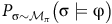
Example 1. Consider a (product) MDP with three states
 $S = \{s_1, s_2, s_3\}$
where
$S = \{s_1, s_2, s_3\}$
where
 $s_1$
is the initial state and
$s_1$
is the initial state and
 $B = \{s_2\}$
is the set of accepting states as shown in Figure 1. In
$B = \{s_2\}$
is the set of accepting states as shown in Figure 1. In
 $s_1$
, the action
$s_1$
, the action
 $\alpha$
leads to
$\alpha$
leads to
 $s_2$
and the action
$s_2$
and the action
 $\beta$
leads to
$\beta$
leads to
 $s_3$
. Since
$s_3$
. Since
 $s_2$
is the only accepting state,
$s_2$
is the only accepting state,
 $\alpha$
is the optimal action that maximizes the expected return. However, there exists a solution to the corresponding Bellman equation suggesting
$\alpha$
is the optimal action that maximizes the expected return. However, there exists a solution to the corresponding Bellman equation suggesting
 $\rm\beta$
is the optimal action, as follows:
$\rm\beta$
is the optimal action, as follows:
 $$\matrix{ {{a^*}} \hfill & \!\!\!\! {:= \mathop {{\rm{argmax}}}\limits_{a\,\in\, \{ \alpha, \beta \} } \{ P(s,a,s')V(s')\} } \hfill \cr {} \hfill & \!\! { = \mathop {{\rm{argmax}}}\limits_{a\,\in\, \{ \alpha, \beta \} } \left\{ {\matrix{ {V({s_2})} \hfill & {{\rm{if }}\quad a = \alpha, } \hfill \cr {V({s_3})} \hfill & {{\rm{if }}\quad a = \beta, } \hfill \cr } } \right.} \hfill \cr } $$
where
 $V(s_2)$
and
$V(s_2)$
and
 $V(s_3)$
can be computed using the Bellman equation (7) as the following:
$V(s_3)$
can be computed using the Bellman equation (7) as the following:
 $$V({s_2}) = 1 - {{\rm\gamma} _B} + {{\rm\gamma} _B}V({s_2}),\quad V({s_3}) = V({s_3}).$$
yielding
 $V(s_2)=1$
and
$V(s_2)=1$
and
 $V(s_3)=c$
where
$V(s_3)=c$
where
 $c\in\mathbb{R}$
is an arbitrary constant. Suppose
$c\in\mathbb{R}$
is an arbitrary constant. Suppose
 $c=2$
is chosen as the solution, then the optimal action will be incorrectly identified as
$c=2$
is chosen as the solution, then the optimal action will be incorrectly identified as
 $\rm\beta$
by (8).
$\rm\beta$
by (8).


Overview of main results
Our work focuses on identifying the true value function among the multiple possible solutions of the Bellman equation. The Bellman equation provides a necessary condition for determining the value function. However, it can have several solutions, with only one being the true value function (for instance, the Bellman equation for reachability (Baier and Katoen, Reference Baier and Katoen2008, P851)).
In Example 1, for
 $c=0$
, the solution for
$c=0$
, the solution for
 $V(s_3)$
is the value function equal to zero since no reward will be collected on this self-loop based on (3). Generally, the solution should be zero for all states in the rejecting BSCCs, as defined below.
$V(s_3)$
is the value function equal to zero since no reward will be collected on this self-loop based on (3). Generally, the solution should be zero for all states in the rejecting BSCCs, as defined below.
Definition 6. A bottom strongly connected component (BSCC) of an MC is a strongly connected component without outgoing transitions (Baier and Katoen, Reference Baier and Katoen2008, P774). The states in and out of the BSCCs are also called recurrent and transient states, respectively. Let B denotes the set of accepting states of the product MDP. A BSCC is rejecting
Footnote
2
if all states
 $s \,\notin\, B$
. Otherwise, we call it an accepting BSCC.
$s \,\notin\, B$
. Otherwise, we call it an accepting BSCC.
By Definition 6, a path that starts in a rejecting BSCC never reaches an accepting state. Thus, the value function for all states in the rejecting BSCCs equals 0 based on (3). Setting the values for all states within a rejecting BSCC to zero is a sufficient condition for the Bellman equation to yield a unique value function, as stated below. (This value function approximates the satisfaction probability defined in (2) and is equal to it when
 ${\rm\gamma}_B \to 1$
.)
${\rm\gamma}_B \to 1$
.)
Theorem 1. The Bellman equation (7) has the value function as the unique solution, if and only if i) the discount factor
 ${\rm\gamma} \lt 1$
or ii) the discount factor
${\rm\gamma} \lt 1$
or ii) the discount factor
 ${\rm\gamma} = 1$
and the solution for any state in a rejecting BSCC is zero.
${\rm\gamma} = 1$
and the solution for any state in a rejecting BSCC is zero.
Methodology
We illustrate the proof of Theorem 1 in this section. Specifically, we first prove it for the case of
 ${\rm\gamma} \lt 1$
and then move to the case of
${\rm\gamma} \lt 1$
and then move to the case of
 ${\rm\gamma}=1$
. The surrogate reward (3) depends on whether a state is an accepting state or not. Thus, we split the state space S by the accepting states B and rejecting states
${\rm\gamma}=1$
. The surrogate reward (3) depends on whether a state is an accepting state or not. Thus, we split the state space S by the accepting states B and rejecting states
 $\neg B:=S\backslash{B}$
. The Bellman equation can be rewritten in the following form,
$\neg B:=S\backslash{B}$
. The Bellman equation can be rewritten in the following form,
 $$\matrix{ {} \hfill & {\left[ {\matrix{ {{V^B}} \cr {{V^{\neg B}}} \cr } } \right] = (1 - {{\rm\gamma} _B})\left[ {\matrix{ {{{\mathbb I}_m}} \cr {{{\mathbb O}_n}} \cr } } \right]} \hfill \cr {} \hfill & {\!\! + \underbrace {\left[ {\matrix{ {{{\rm\gamma} _B}{I_{m \times m}}} & {} \cr {} & {{\rm\gamma} {I_{n \times n}}} \cr } } \right]}_{{\Gamma _B}}\underbrace {\left[ {\matrix{ {{P_{\pi, B \to B}}} & {{P_{\pi, B \to \neg B}}} \cr {{P_{\pi, \neg B \to B}}} & {{P_{\pi, \neg B \to \neg B}}} \cr } } \right]}_{{P_\pi }}\left[ {\matrix{ {{V^B}} \cr {{V^{\neg B}}} \cr } } \right],} \hfill \cr } $$
where
 $m=\vert B\vert$
,
$m=\vert B\vert$
,
 $n=\vert \neg B \vert$
,
$n=\vert \neg B \vert$
,
 $V^{B}\in\mathbb{R}^{m}$
,
$V^{B}\in\mathbb{R}^{m}$
,
 $V^{\neg B}\in\mathbb{R}^n$
are the vectors listing the value function for all
$V^{\neg B}\in\mathbb{R}^n$
are the vectors listing the value function for all
 $s\in {B}$
and
$s\in {B}$
and
 $s\in {\neg B}$
, respectively.
$s\in {\neg B}$
, respectively.
 $\mathbb{I}$
and
$\mathbb{I}$
and
 $\mathbb{O}$
are column vectors with all 1 and 0 elements, respectively. Each of the matrices
$\mathbb{O}$
are column vectors with all 1 and 0 elements, respectively. Each of the matrices
 $P_{\pi,B\rightarrow B}$
,
$P_{\pi,B\rightarrow B}$
,
 $ P_{\pi,B\rightarrow \neg B}$
,
$ P_{\pi,B\rightarrow \neg B}$
,
 $P_{\pi,\neg B\rightarrow B}$
,
$P_{\pi,\neg B\rightarrow B}$
,
 $P_{\pi,\neg B\rightarrow \neg B}$
contains the transition probability from a set of states to a set of states, their combination is the transition matrix
$P_{\pi,\neg B\rightarrow \neg B}$
contains the transition probability from a set of states to a set of states, their combination is the transition matrix
 $P_\pi$
for the induced MC. In the following, we assume a fixed policy
$P_\pi$
for the induced MC. In the following, we assume a fixed policy
 $\pi$
, leading us to omit the
$\pi$
, leading us to omit the
 $\pi$
subscript from most notation when its implication is clear from the context.
$\pi$
subscript from most notation when its implication is clear from the context.
The case
${\rm\gamma} \lt 1$

Proposition 1. If
 ${\rm\gamma} \lt 1$
in the surrogate reward (3), then the Bellman equation (10) has the value function as the unique solution.
${\rm\gamma} \lt 1$
in the surrogate reward (3), then the Bellman equation (10) has the value function as the unique solution.
As
 ${\rm\gamma} \lt 1$
, the invertibility of
${\rm\gamma} \lt 1$
, the invertibility of
 $(I-\Gamma_B P_\pi)$
can be shown by applying Gershgorin circle theorem (Bell, Reference Bell1965, Theorem 0) to
$(I-\Gamma_B P_\pi)$
can be shown by applying Gershgorin circle theorem (Bell, Reference Bell1965, Theorem 0) to
 $\Gamma_B P_\pi$
. Specifically, any eigenvalue
$\Gamma_B P_\pi$
. Specifically, any eigenvalue
 $\lambda$
of
$\lambda$
of
 $\Gamma_B P_\pi$
satisfies
$\Gamma_B P_\pi$
satisfies
 $|\lambda | \lt 1$
since each row sum of
$|\lambda | \lt 1$
since each row sum of
 $\Gamma_B P_\pi$
is strictly less than 1. Then, the solution for the Bellman equation (10) can be uniquely determined as
$\Gamma_B P_\pi$
is strictly less than 1. Then, the solution for the Bellman equation (10) can be uniquely determined as
 $$\matrix{ {\left[ {\matrix{ {{V^B}} \cr {{V^{\neg B}}} \cr } } \right]} \hfill & {\!\!\!\!\! = (1 - {{\rm\gamma} _B}){{({I_{m + n}} - {\Gamma _B}{P_\pi })}^{ - 1}}\left[ {\matrix{ {{{\mathbb I}_m}} \cr {{{\mathbb O}_n}} \cr } } \right].} \hfill \cr } $$
Proof. The solution of the Bellman equation (10) can be determined uniquely by matrix operation (11) if
 $(I-\Gamma_B P_\pi)$
is invertible. The invertibility is shown using the Gershgorin circle theorem (Bell, Reference Bell1965, Theorem 0), which claims the following. For a square matrix A, define the radius as
$(I-\Gamma_B P_\pi)$
is invertible. The invertibility is shown using the Gershgorin circle theorem (Bell, Reference Bell1965, Theorem 0), which claims the following. For a square matrix A, define the radius as
 $r_i:=\sum_{j\ne i}{\vert A_{ij}\vert}$
. Then, each eigenvalue of A is in at least one of the Gershgorin disks
$r_i:=\sum_{j\ne i}{\vert A_{ij}\vert}$
. Then, each eigenvalue of A is in at least one of the Gershgorin disks
 ${\mathcal D}(A_{ii},r_i):=\{z:\vert z-A_{ii}\vert\le r_i\}$
.
${\mathcal D}(A_{ii},r_i):=\{z:\vert z-A_{ii}\vert\le r_i\}$
.
For the matrix
 $\Gamma_B P_\pi$
, at its i-th row, we have the center of the disk as
$\Gamma_B P_\pi$
, at its i-th row, we have the center of the disk as
 $(\Gamma_B P_\pi)_{ii}=(\Gamma_B)_{ii}{(P_\pi)}_{ii}$
, and the radius as
$(\Gamma_B P_\pi)_{ii}=(\Gamma_B)_{ii}{(P_\pi)}_{ii}$
, and the radius as
 $r_i=\sum_{j\ne i}{\vert (\Gamma_B P_\pi)_{ij}\vert} ={(\Gamma_B)}_{ii}(1-{(P_\pi)}_{ii})$
. We can upper bound the disk as
$r_i=\sum_{j\ne i}{\vert (\Gamma_B P_\pi)_{ij}\vert} ={(\Gamma_B)}_{ii}(1-{(P_\pi)}_{ii})$
. We can upper bound the disk as
 $$\matrix{ {{\cal D}({{({\Gamma _B}{P_\pi })}_{ii}},{r_i})} \hfill & {\!\!\!\! = \{ z:|z - {{({\Gamma _B}{P_\pi })}_{ii}}| \le {r_i}\} } \hfill \cr {} \hfill & \!\! \!\!{ \subseteq \{ z:|z| \le {{({\Gamma _B}{P_\pi })}_{ii}} + {r_i}\} } \hfill \cr {} \hfill & \!\! \!\!{ \subseteq \{ z:|z| \le {\rm\gamma} \} .} \hfill \cr } $$
Since all Gershgorin disks share the same upper bound, the union of all disks is also bounded by
 $$\bigcup\limits_{i\,\in\, S} {{\cal D}({{({\Gamma _B}{P_\pi })}_{ii}},{r_i})} \subseteq \{ z:|z| \le {\rm\gamma} \} .$$
The inequality
 ${\rm\gamma} \lt 1$
ensures that any eigenvalue
${\rm\gamma} \lt 1$
ensures that any eigenvalue
 $\lambda$
of
$\lambda$
of
 $\Gamma_B P$
satisfies
$\Gamma_B P$
satisfies
 $|\lambda | \lt 1$
. Thus
$|\lambda | \lt 1$
. Thus
 $(I-\Gamma_B P_\pi)$
is invertible and the solution can be uniquely determined by (11). The value function satisfies the Bellman equation (10), which has a unique solution, which is the value function. Thus, the proposition holds.
$(I-\Gamma_B P_\pi)$
is invertible and the solution can be uniquely determined by (11). The value function satisfies the Bellman equation (10), which has a unique solution, which is the value function. Thus, the proposition holds.
 $\square$
The case
${\rm\gamma}=1$

For
 ${\rm\gamma}=1$
, the matrix
${\rm\gamma}=1$
, the matrix
 $(I-\Gamma_B P_\pi)$
may not be invertible, causing the Bellman equation (10) to have multiple solutions. Since the solution may not be the value function here, we use
$(I-\Gamma_B P_\pi)$
may not be invertible, causing the Bellman equation (10) to have multiple solutions. Since the solution may not be the value function here, we use
 $U^{B}\in \mathbb{R}^m$
and
$U^{B}\in \mathbb{R}^m$
and
 $U^{\neg B}\in \mathbb{R}^n$
to represent a solution on states in B and
$U^{\neg B}\in \mathbb{R}^n$
to represent a solution on states in B and
 $\neg B$
, respectively. In an induced MC, a path starts in an initial state, travels finite steps among the transient states, and eventually enters a BSCC. If the induced MC has only accepting BSCCs, the connection between all states in B can be captured by a new transition matrix, and the Bellman operator is contractive on the states in B. Thus, we can show the solution is unique in all the states in the following subsection. In the general case where rejecting BSCCs also exists, we introduce a sufficient condition of fixing all solutions within rejecting BSCCs to zero. We demonstrate the uniqueness of the solution under this condition first on
$\neg B$
, respectively. In an induced MC, a path starts in an initial state, travels finite steps among the transient states, and eventually enters a BSCC. If the induced MC has only accepting BSCCs, the connection between all states in B can be captured by a new transition matrix, and the Bellman operator is contractive on the states in B. Thus, we can show the solution is unique in all the states in the following subsection. In the general case where rejecting BSCCs also exists, we introduce a sufficient condition of fixing all solutions within rejecting BSCCs to zero. We demonstrate the uniqueness of the solution under this condition first on
 $U^{B}$
and then on
$U^{B}$
and then on
 $U^{\neg B}$
in the second part of this section.
$U^{\neg B}$
in the second part of this section.
When the MC only has accepting BSCCs
This section focuses on proving that the Bellman equation (10) has a unique solution when there are no rejecting BSCCs in the MC. The result is as follows,
Proposition 2. If the MC only has accepting BSCCs (i.e., no rejecting BSCCs) and
 ${\rm\gamma}=1$
in the surrogate reward (3), then the Bellman equation (10) has a unique solution
${\rm\gamma}=1$
in the surrogate reward (3), then the Bellman equation (10) has a unique solution
 $[{U^B}^T, {U^{\neg B}}^T]^T= \mathbb{I}$
.
$[{U^B}^T, {U^{\neg B}}^T]^T= \mathbb{I}$
.
The intuition behind the proof is to capture the connection between all states B by a new transition matrix
 $P_\pi^B$
in Lemma 3. Then, one can use
$P_\pi^B$
in Lemma 3. Then, one can use
 $I-{\rm\gamma}_B P_\pi^B$
is invertible to show the solutions
$I-{\rm\gamma}_B P_\pi^B$
is invertible to show the solutions
 $U_B$
is unique and furthermore, show
$U_B$
is unique and furthermore, show
 $U^{\neg B}$
is uniquely determined by
$U^{\neg B}$
is uniquely determined by
 $U^{B}$
in Lemma 4.
$U^{B}$
in Lemma 4.
Lemma 3. If the MC
 ${\mathcal{M}}_\pi=(S, P_\pi, s_{\rm 0},\Lambda, L)$
only has accepting BSCCs, one can represent the transitions between accepting states as an MC with only accepting states
${\mathcal{M}}_\pi=(S, P_\pi, s_{\rm 0},\Lambda, L)$
only has accepting BSCCs, one can represent the transitions between accepting states as an MC with only accepting states
 ${\mathcal M}_\pi^B:=(B, P_\pi^B,\mu,\Lambda, L)$
where
${\mathcal M}_\pi^B:=(B, P_\pi^B,\mu,\Lambda, L)$
where
-
B is the set of accepting states,
-
$P_\pi^B$
is the transition probability matrix defined by(14)
$$P_\pi ^B: = {P_{\pi, B \to B}} + {P_{\pi, B \to \neg B}}{(I - {P_{\pi, \neg B \to \neg B}})^{ - 1}}{P_{\pi, \neg B \to B}}.$$
-
$\mu\,\in\, \Delta(B)$
is the initial distribution and determined by
$s_0$
as(15)where
$$\eqalign{ & {\rm{if}}\;{\mkern 1mu} {s_0}\,\in\, B,\quad \mu (s) = \left\{ {\matrix{ 1 \hfill & {s = {s_0}} \hfill \cr 0 \hfill & {s \ne {s_0}} \hfill \cr } } \right., \cr & {\rm{if}}\;{\mkern 1mu} {s_0} \;\notin\; B,\quad \mu (s) = {({P_{init}})_{{s_0}s}} \cr} $$
$P_{init} := (I-P_{\pi,\neg B\to \neg B})^{-1}P_{\pi,\neg B\to B}$
is a matrix. Each element
$(P_{init})_{ij}$
represents the probability of a path leaving the state
$i\in {\neg B}$
and visiting state
$j\in B$
without visiting any state in B between the leave and visit.


Proof. We start with constructing a transition matrix
 $P_\pi^B$
for the states in B whose (i, j)th element, denoted by
$P_\pi^B$
for the states in B whose (i, j)th element, denoted by
 $(P_\pi^B)_{ij}$
, is the probability of visiting jth state in B without visiting any state in B after leaving the ith state in B.
$(P_\pi^B)_{ij}$
, is the probability of visiting jth state in B without visiting any state in B after leaving the ith state in B.
 $$\matrix{ {P_\pi ^B} \hfill & {\!\!\!\!: = {P_{\pi, B \to B}} + {P_{\pi, B \to \neg B}}\sum\limits_{k = 0}^\infty {P_{\pi, \neg B \to \neg B}^k} {P_{\pi, \neg B \to B}}.} \hfill \cr } $$
In (16), the matrix element
 $(P_{\pi,\neg B\to \neg B}^k)_{ij}$
represents the probability of a path leaving the state i and visiting state j after k steps without travelling through any states in B. However, the absence of rejecting BSCCs ensures that any path will visit a state in B in finite times with probability 1. Thus, for any
$(P_{\pi,\neg B\to \neg B}^k)_{ij}$
represents the probability of a path leaving the state i and visiting state j after k steps without travelling through any states in B. However, the absence of rejecting BSCCs ensures that any path will visit a state in B in finite times with probability 1. Thus, for any
 $i, j\,\in\, \neg B$
,
$i, j\,\in\, \neg B$
,
 $\lim_{k\to \infty}(P_{\pi,\neg B\to \neg B}^k)_{ij}=0$
. This limit implies any eigenvalue
$\lim_{k\to \infty}(P_{\pi,\neg B\to \neg B}^k)_{ij}=0$
. This limit implies any eigenvalue
 $\lambda$
of
$\lambda$
of
 $P_{\pi,\neg B\to \neg B}$
satisfies
$P_{\pi,\neg B\to \neg B}$
satisfies
 $|\lambda | \lt 1$
and therefore
$|\lambda | \lt 1$
and therefore
 $\sum\nolimits_{k = 0}^\infty {P_{\pi, \neg B \to \neg B}^k} $
can be replaced by
$\sum\nolimits_{k = 0}^\infty {P_{\pi, \neg B \to \neg B}^k} $
can be replaced by
 $(I - P_{\pi,\neg B\rightarrow \neg B})^{-1}$
in (16),
$(I - P_{\pi,\neg B\rightarrow \neg B})^{-1}$
in (16),
 $$P_\pi ^B = {P_{\pi, B \to B}} + {P_{\pi, B \to \neg B}}{(I - {P_{\pi, \neg B \to \neg B}})^{ - 1}}{P_{\pi, \neg B \to B}}.$$
Since all the elements on the right-hand side are greater or equal to zero, for any
 $i, j\,\in\, B$
,
$i, j\,\in\, B$
,
 $(P_\pi^B)_{ij}\ge 0$
. Since there are only accepting BSCCs in the MC, given a path starting from an arbitrary state in B, the path will visit an accepting state in finite steps with probability one, ensuring that for all
$(P_\pi^B)_{ij}\ge 0$
. Since there are only accepting BSCCs in the MC, given a path starting from an arbitrary state in B, the path will visit an accepting state in finite steps with probability one, ensuring that for all
 $i\in B$
,
$i\in B$
,
 $\sum_{j\in S} (P_\pi^B)_{ij}=1$
. Thus,
$\sum_{j\in S} (P_\pi^B)_{ij}=1$
. Thus,
 $P_\pi^B$
is a probability matrix that can be used to describe the behaviour of an MC with the state space as B only.
$P_\pi^B$
is a probability matrix that can be used to describe the behaviour of an MC with the state space as B only.
Lemma 4. Suppose there is no rejecting BSCC, for
 ${\rm\gamma} =1$
in (3), the Bellman equation (10) is equivalent to the following form,
${\rm\gamma} =1$
in (3), the Bellman equation (10) is equivalent to the following form,
 $$\matrix{ {} \hfill & {\left[ {\matrix{ {{U^B}} \cr {{U^{\neg B}}} \cr } } \right] = (1 - {{\rm\gamma} _B})\left[ {\matrix{ {{{\mathbb I}_m}} \cr {{{\mathbb O}_n}} \cr } } \right]} \hfill \cr {} \hfill & {\!\! + \left[ {\matrix{ {{{\rm\gamma} _B}{I_{m \times m}}} & {} \cr {} & {{I_{n \times n}}} \cr } } \right]\left[ {\matrix{ {P_\pi ^B} & {} \cr {{P_{\pi, \neg B \to B}}} & {{P_{\pi, \neg B \to \neg B}}} \cr } } \right]\left[ {\matrix{ {{U^B}} \cr {{U^{\neg B}}} \cr } } \right].} \hfill \cr } $$
The equation (18) implies that the solution
 $U^{B}$
does not rely on the rejecting states
$U^{B}$
does not rely on the rejecting states
 $\neg B$
. Subsequently, we leverage the fact that
$\neg B$
. Subsequently, we leverage the fact that
 $U^{\neg B}$
is uniquely determined by
$U^{\neg B}$
is uniquely determined by
 $U^{B}$
to establish the uniqueness of the overall solution V.
$U^{B}$
to establish the uniqueness of the overall solution V.
Proof. We prove this lemma by showing the equivalence between
 $P_\pi^B U^{B}$
and
$P_\pi^B U^{B}$
and
 $P_{\pi,B\to B}U^{B} + P_{\pi,B\to\neg B}U^{\neg B}$
. From the Bellman equation (10), we have
$P_{\pi,B\to B}U^{B} + P_{\pi,B\to\neg B}U^{\neg B}$
. From the Bellman equation (10), we have
 $U^{\neg B}=P_{\pi,\neg B\to B} U^{B} + P_{\pi,\neg B\to \neg B}U^{\neg B}$
 $$\eqalign{ & {P_{\pi, B \to B}}{U^B} + {P_{\pi, B \to \neg B}}{U^{\neg B}} \cr & \mathop = \limits^{\unicode{x24B6}} \left( {{P_{\pi, B \to B}} + {P_{\pi, B \to \neg B}}{P_{\pi, \neg B \to B}}} \right){U^B} \cr & + {P_{\pi, B \to \neg B}}{P_{\pi, \neg B \to \neg B}}{U^{\neg B}} \cr & \mathop = \limits^{\unicode{x24B7}} \left( {{P_{\pi, B \to B}} + {P_{\pi, B \to \neg B}}{P_{\pi, \neg B \to B}}} \right){U^B} \cr & + \left( {{P_{\pi, B \to \neg B}}{P_{\pi, \neg B \to \neg B}}{P_{\pi, \neg B \to B}}} \right){U^B} \cr & + {P_{\pi, B \to \neg B}}P_{\pi, \neg B \to \neg B}^2{U^{\neg B}} \cr & \vdots \cr & \mathop = \limits^{ \unicode{x24B8}} \mathop {{\rm{lim}}}\limits_{ K \to \infty } \Bigg(\left( {{P_{\pi, B \to B}} + {P_{\pi, B \to \neg B}}\mathop \sum \limits_{k = 0}^K P_{\pi, \neg B \to \neg B}^{k}{P_{\pi, \neg B \to B}}} \right){U^B} \cr & + {P_{\pi, B \to \neg B}}P_{\pi, \neg B \to \neg B}^{K + 1}{U^{\neg B}}\Bigg) \cr & \mathop = \limits^\unicode{x24B9} P_\pi ^B{U^B} \cr} $$
where the equality Ⓐ holds as we replace
 $U^{\neg B}$
in the last term
$U^{\neg B}$
in the last term
 $P_{\pi,B\to\neg B}U^{\neg B}$
by
$P_{\pi,B\to\neg B}U^{\neg B}$
by
 $P_{\pi,\neg B\to B} U^{B} + P_{\pi,\neg B\to \neg B}U^{\neg B}$
. Similarily, the equalities Ⓑ and Ⓒ hold as we keep replacing
$P_{\pi,\neg B\to B} U^{B} + P_{\pi,\neg B\to \neg B}U^{\neg B}$
. Similarily, the equalities Ⓑ and Ⓒ hold as we keep replacing
 $U^{\neg B}$
in the last term by
$U^{\neg B}$
in the last term by
 $P_{\pi,\neg B\to B} U^{B} + P_{\pi,\neg B\to \neg B}U^{\neg B}$
. The equality Ⓓ holds by the definition of
$P_{\pi,\neg B\to B} U^{B} + P_{\pi,\neg B\to \neg B}U^{\neg B}$
. The equality Ⓓ holds by the definition of
 $P_\pi^B$
.
$P_\pi^B$
.
 $\square$
Lemma 4 shows the uniqueness of the solution. Directly solving equation (18) completes the proof for Proposition 2.
Proof for Proposition 2. From equation (18), we obtain the expression for the MC with only accepting states,
 $${U^B} = (1 - {{\rm\gamma} _B}){\mathbb I} + {{\rm\gamma} _B}P_\pi ^B{U^B}.$$
Given that all the eigenvalues of
 $P_\pi^B$
are within the unit disk and
$P_\pi^B$
are within the unit disk and
 ${{\rm\gamma} _B} \lt 1$
, the matrix
${{\rm\gamma} _B} \lt 1$
, the matrix
 $(I-{\rm\gamma}_B P_\pi^B)$
is invertible.
$(I-{\rm\gamma}_B P_\pi^B)$
is invertible.
 $U^{B}$
is uniquely determined by
$U^{B}$
is uniquely determined by
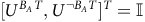
 $${U^B} = (1 - {{\rm\gamma} _B}){(I - {{\rm\gamma} _B}P_\pi ^B)^{ - 1}}{\mathbb I}.$$
Moving to the set of rejecting states
 $U^{\neg B}$
, from equation (18) we have,
$U^{\neg B}$
, from equation (18) we have,
 $$\matrix{ {{U^{\neg B}}} \hfill & {\!\!\!\! = {P_{\pi, \neg B \to B}}{U^B} + {P_{\pi, \neg B \to \neg B}}{U^{\neg B}}} \hfill \cr {} \hfill & {\!\! \!\!= {{(I - {P_{\pi, \neg B \to \neg B}})}^{ - 1}}{P_{\pi, \neg B \to B}}{U^B}.} \hfill \cr } $$
Given the uniqueness of
 $U^{B}$
, and the invertibility of
$U^{B}$
, and the invertibility of
 $(I-P_{\pi,\neg B\rightarrow \neg B})$
, we conclude that
$(I-P_{\pi,\neg B\rightarrow \neg B})$
, we conclude that
 $U^{\neg B}$
is also unique.
$U^{\neg B}$
is also unique.
Let
 $U^{B}=\mathbb{I}_m$
and
$U^{B}=\mathbb{I}_m$
and
 $U^{\neg B}=\mathbb{I}_n$
, the Bellman equation (10) holds as the summation of each row of a probability matrix
$U^{\neg B}=\mathbb{I}_n$
, the Bellman equation (10) holds as the summation of each row of a probability matrix
 $P_B$
is always one,
$P_B$
is always one,
 $$\matrix{ {\left[ {\matrix{ {{{\mathbb I}_m}} \cr {{{\mathbb I}_n}} \cr } } \right]} \hfill & {\!\! = (1 - {{\rm\gamma} _B})\left[ {\matrix{ {{{\mathbb I}_m}} \cr {{{\mathbb O}_n}} \cr } } \right] + \left[ {\matrix{ {{{\rm\gamma} _B}{I_{m \times m}}} & {} \cr {} & {{I_{n \times n}}} \cr } } \right]{P_\pi }\left[ {\matrix{ {{{\mathbb I}_m}} \cr {{{\mathbb I}_n}} \cr } } \right].} \hfill \cr } $$
Therefore, in the absence of rejecting BSCCs, the unique solution to the Bellman equation (10) is
 $\mathbb{I}$
.
$\mathbb{I}$
.
 $\square$
Proposition 2 shows the solutions for the states inside an accepting BSCC have to be 1. All states outside the BSCC cannot be reached from a state inside the BSCC, thus the solution for states outside this BSCC is not involved in the solution for states inside the BSCC. By Lemma 4, the Bellman equation for an accepting BSCC can be rewritten into the form of (18) where
 $U_B$
and
$U_B$
and
 $U_{\neg B}$
stands for the solution for accepting states and rejecting states inside this BSCC, and vector
$U_{\neg B}$
stands for the solution for accepting states and rejecting states inside this BSCC, and vector
 $\mathbb{I}$
is the unique solution.
$\mathbb{I}$
is the unique solution.
When accepting and rejecting BSCC both exist in the MC
Having established the uniqueness of solutions in the case of accepting BSCCs, we now shift our focus to the general case involving rejecting BSCCs. We state in Proposition 2 that the solutions for the states in the accepting BSCCs are unique and equal to
 $\mathbb{I}$
. We now demonstrate that setting the solutions for the states in rejecting BSCCs to
$\mathbb{I}$
. We now demonstrate that setting the solutions for the states in rejecting BSCCs to
 $\mathbb{O}$
ensures the uniqueness and correctness of the solutions for all states. We partition the state space further into
$\mathbb{O}$
ensures the uniqueness and correctness of the solutions for all states. We partition the state space further into
 $\{B_A, B_T, \neg B_A, \neg B_R, \neg B_T\}$
. Here the subscripts A and R denote accepting and rejecting (unrelated to the action set A or reward function R). Specifically,
$\{B_A, B_T, \neg B_A, \neg B_R, \neg B_T\}$
. Here the subscripts A and R denote accepting and rejecting (unrelated to the action set A or reward function R). Specifically,
-
$B_A$
is the set of accepting states in the BSCCs,
-
$B_T:=B\backslash B_A$
is the set of transient accepting states,
-
$\neg B_A$
is the set of rejecting states in the accepting BSCCs,
-
$\neg B_R$
is the set of rejecting states in the rejecting BSCCs,
-
$\neg B_T:=\neg B\backslash (\neg B_A \cup \neg B_R)$
is set of transient rejecting states.


We rewrite the Bellman equation (10) in the form of (24).
 $${\matrix{ {} \hfill & {\left[ {\matrix{ {{U^{{B_T}}}} \cr {{U^{{B_A}}}} \cr {{U^{\neg {B_T}}}} \cr {{U^{\neg {B_A}}}} \cr {{U^{\neg {B_R}}}} \cr } } \right] = (1 - {{\rm\gamma} _B})\left[ {\matrix{ {{{\mathbb I}_m}} \cr {{{\mathbb O}_n}} \cr } } \right]} \hfill \cr {} \hfill & \!\!\!\!\!\!{ + \left[ {\matrix{ {{{\rm\gamma} _B}{I_{m \times m}}} & {} \cr {} & {{I_{n \times n}}} \cr } } \right]} \hfill \cr {} \hfill & \!\!\!\!\!\!\!\times{\left[ {\matrix{ {{P_{\pi, {B_T} \to {B_T}}}} & {{P_{\pi, {B_T} \to {B_A}}}} & {{P_{\pi, {B_T} \to \neg {B_T}}}} & {{P_{\pi, {B_T} \to \neg {B_A}}}} & {{P_{\pi, {B_T} \to \neg {B_R}}}} \cr {} & {{P_{\pi, {B_A} \to {B_A}}}} & {} & {{P_{\pi, {B_A} \to \neg {B_A}}}} & {{P_{\pi, {B_A} \to \neg {B_R}}}} \cr {{P_{\pi, \neg {B_T} \to {B_T}}}} & {{P_{\pi, \neg {B_T} \to {B_A}}}} & {{P_{\pi, \neg {B_T} \to \neg {B_T}}}} & {{P_{\pi, \neg {B_T} \to \neg {B_A}}}} & {{P_{\pi, \neg {B_T} \to \neg {B_R}}}} \cr {} & {{P_{\pi, \neg {B_A} \to {B_A}}}} & {} & {{P_{\pi, \neg {B_A} \to \neg {B_A}}}} & {{P_{\pi, \neg {B_A} \to \neg {B_R}}}} \cr {} & {} & {} & {} & {{P_{\pi, \neg {B_R} \to \neg {B_R}}}} \cr } } \right]} \hfill \cr {} \hfill & \!\!\!\!\!\times{\left[ {\matrix{ {{U^{{B_T}}}} \cr {{U^{{B_A}}}} \cr {{U^{\neg {B_T}}}} \cr {{U^{\neg {B_A}}}} \cr {{U^{\neg {B_R}}}} \cr } } \right].} \hfill \cr }} $$
The solution for states inside BSCCs has been fixed as
 $[{U^{B_A}}^T, {U^{\neg B_A}}^T]^T=\mathbb{I}$
and
$[{U^{B_A}}^T, {U^{\neg B_A}}^T]^T=\mathbb{I}$
and
 $U^{\neg B_R}=\mathbb{O}$
. The solution
$U^{\neg B_R}=\mathbb{O}$
. The solution
 $U^{B_T}$
and
$U^{B_T}$
and
 $U^{\neg B_T}$
for transient states remain to be shown as unique. We rewrite the Bellman equation (24) into the following form (25) where
$U^{\neg B_T}$
for transient states remain to be shown as unique. We rewrite the Bellman equation (24) into the following form (25) where
 $U^{B_T}$
and
$U^{B_T}$
and
 $U^{\neg B_T}$
are the only variables,
$U^{\neg B_T}$
are the only variables,
 $$\matrix{ {} \hfill & {\left[ {\matrix{ {{U^{{B_T}}}} \cr {{U^{\neg {B_T}}}} \cr } } \right] = \left[ {\matrix{ {{{\rm\gamma} _B}{I_{{m_1} \times {m_1}}}} & {} \cr {} & {{I_{{n_1} \times {n_1}}}} \cr } } \right]} \hfill \cr {} \hfill & {\left[ {\matrix{ {{P_{\pi, {B_T} \to {B_T}}}} & {{P_{\pi, {B_T} \to \neg {B_T}}}} \cr {{P_{\pi, \neg {B_T} \to {B_T}}}} & {{P_{\pi, \neg {B_T} \to \neg {B_T}}}} \cr } } \right]\left[ {\matrix{ {{U^{{B_T}}}} \cr {{U^{\neg {B_T}}}} \cr } } \right] + \left[ {\matrix{ {{B_1}} \cr {{B_2}} \cr } } \right]} \hfill \cr } $$
here
 $m_1=\vert U^{B_T}\vert$
,
$m_1=\vert U^{B_T}\vert$
,
 $m_2=\vert U^{B_A}\vert$
,
$m_2=\vert U^{B_A}\vert$
,
 $n_1=\vert U^{\neg B_T}\vert$
,
$n_1=\vert U^{\neg B_T}\vert$
,
 $n_2=\vert U^{\neg B_A}\vert$
, and
$n_2=\vert U^{\neg B_A}\vert$
, and
 $$\eqalign{ & \left[ {\matrix{ {{B_1}} \cr {{B_2}} \cr } } \right] = (1 - {{\rm\gamma} _B})\left[ {\matrix{ {{{\mathbb I}_{{m_1}}}} \cr {{{\mathbb O}_{{n_1}}}} \cr } } \right] + \left[ {\matrix{ {{{\rm\gamma} _B}{I_{{m_1} \times {m_1}}}} & {} \cr {} & {{I_{{n_1} \times {n_1}}}} \cr } } \right] \cr & \left[ {\matrix{ {{P_{\pi, {B_T} \to {B_A}}}} & {{P_{\pi, {B_T} \to \neg {B_A}}}} \cr {{P_{\pi, \neg {B_T} \to {B_A}}}} & {{P_{\pi, \neg {B_T} \to \neg {B_A}}}} \cr } } \right]\left[ {\matrix{ {{{\mathbb I}_{{m_2}}}} \cr {{{\mathbb I}_{{n_2}}}} \cr } } \right]. \cr} $$
Lemma 5. The equation (25) has a unique solution.
We demonstrate
 $U^{B_T}$
does not rely on states in
$U^{B_T}$
does not rely on states in
 $\neg B_T$
and
$\neg B_T$
and
 $U^{\neg B_T}$
is uniquely determined by
$U^{\neg B_T}$
is uniquely determined by
 $U^{B_T}$
. Then the uniqueness of
$U^{B_T}$
. Then the uniqueness of
 $U^{B_T}$
can be shown first, consequently, uniqueness of
$U^{B_T}$
can be shown first, consequently, uniqueness of
 $U^{\neg B_T}$
can be shown.
$U^{\neg B_T}$
can be shown.
Proof. First we show
 $U^{B_T}$
is unique since its calculation can exclude
$U^{B_T}$
is unique since its calculation can exclude
 $U^{\neg B}$
. By equation (25),
$U^{\neg B}$
. By equation (25),
 $$\matrix{ {{U^{\neg {B_T}}}} \hfill & {\!\! \!\!= {P_{\pi, \neg {B_T} \to {B_T}}}{U^{{B_T}}} + {P_{\pi, \neg {B_T} \to \neg {B_T}}}{U^{\neg {B_T}}}} \hfill \cr\cr {} \hfill & {\!\!\!\! + \left[ {\matrix{ {{P_{\pi, \neg {B_T} \to {B_A}}}} & {{P_{\pi, \neg {B_T} \to \neg {B_A}}}} \cr } } \right]{\mathbb I}} \hfill \cr } $$
The following equalities hold as we keep expanding
 $U^{\neg B_T}$
,
$U^{\neg B_T}$
,
 $$\eqalign{ & {P_{\pi, {B_T} \to {B_T}}}{U^{{B_T}}} + {P_{\pi, {B_T} \to \neg {B_T}}}{U^{\neg {B_T}}} \cr & \mathop = \limits^{\unicode{x24B6}} ({P_{\pi, {B_T} \to {B_T}}} + {P_{\pi, {B_T} \to \neg {B_T}}}{P_{\pi, \neg {B_T} \to {B_T}}}){U^{{B_T}}} \cr & + {P_{\pi, {B_T} \to \neg {B_T}}}\left[ {\matrix{ {{P_{\pi, \neg {B_T} \to {B_A}}}} & {{P_{\pi, \neg {B_T} \to \neg {B_A}}}} \cr } } \right]{\mathbb I} \cr & + {P_{\pi, {B_T} \to \neg {B_T}}}{P_{\pi, \neg {B_T} \to \neg {B_T}}}{U^{\neg {B_T}}} \cr & \vdots \cr & \mathop = \limits^{\unicode{x24B7}} ({P_{\pi, {B_T} \to {B_T}}} + \cr & {P_{\pi, {B_T} \to \neg {B_T}}}\sum\limits_{k = 0}^K {P_{\pi, \neg {B_T} \to \neg {B_T}}^k} {P_{\pi, \neg {B_T} \to {B_T}}}){U^{{B_T}}} \cr & + {P_{\pi, {B_T} \to \neg {B_T}}}\sum\limits_{k = 0}^K {P_{\pi, \neg {B_T} \to \neg {B_T}}^k} \cr & \left[ {\matrix{ {{P_{\pi, \neg {B_T} \to {B_A}}}} & {{P_{\pi, \neg {B_T} \to \neg {B_A}}}} \cr } } \right]{\mathbb I} \cr & + {P_{\pi, {B_T} \to \neg {B_T}}}P_{\pi, \neg {B_T} \to \neg {B_T}}^{K + 1}{U^{\neg {B_T}}} \cr} $$
where the equality Ⓐ holds as we replace
 $U^{\neg B_T}$
in the last term by (26). Similarily, the equality Ⓑ hold as we keep expanding
$U^{\neg B_T}$
in the last term by (26). Similarily, the equality Ⓑ hold as we keep expanding
 $U^{\neg B_T}$
in the last term by (26). Since
$U^{\neg B_T}$
in the last term by (26). Since
 $P_{\pi,\neg B_T\to\neg B_T}$
only contains the transition probabilities between the transient states, for any
$P_{\pi,\neg B_T\to\neg B_T}$
only contains the transition probabilities between the transient states, for any
 $i,j\in \neg B_T$
,
$i,j\in \neg B_T$
,
 $\lim_{K\to\infty}{(P_{\pi,\neg B_T\to\neg B_T}^K)_{ij}}=0$
. Taking
$\lim_{K\to\infty}{(P_{\pi,\neg B_T\to\neg B_T}^K)_{ij}}=0$
. Taking
 $K\to \infty$
in (26) and using the fact that
$K\to \infty$
in (26) and using the fact that
 $(I-P_{\pi,\neg B_T\to\neg B_T})^{-1} = \sum_{k=0}^\infty{P_{\pi,\neg B_T\to\neg B_T}^k}$
, we have
$(I-P_{\pi,\neg B_T\to\neg B_T})^{-1} = \sum_{k=0}^\infty{P_{\pi,\neg B_T\to\neg B_T}^k}$
, we have
 $$\matrix{ {} \hfill & {{P_{\pi, {B_T} \to {B_T}}}{U^{{B_T}}} + {P_{\pi, {B_T} \to \neg {B_T}}}{U^{\neg {B_T}}}} \hfill \cr = \hfill & {({P_{\pi, {B_T} \to {B_T}}} + } \hfill \cr {} \hfill & {{P_{\pi, {B_T} \to \neg {B_T}}}{{(I - {P_{\pi, \neg {B_T} \to \neg {B_T}}})}^{ - 1}}{P_{\pi, \neg {B_T} \to {B_T}}}){U^{{B_T}}}} \hfill \cr + \hfill & {{P_{\pi, {B_T} \to \neg {B_T}}}{{(I - {P_{\pi, \neg {B_T} \to \neg {B_T}}})}^{ - 1}}} \hfill \cr {} \hfill & {\left[ {\matrix{ {{P_{\pi, \neg {B_T} \to {B_A}}}} & {{P_{\pi, \neg {B_T} \to \neg {B_A}}}} \cr } } \right]{\mathbb I}.} \hfill \cr } $$
Plugging (28) into (25), we show the calculation of
 $U^{B_T}$
does not rely on
$U^{B_T}$
does not rely on
 $U^{\neg B}$
,
$U^{\neg B}$
,
 $$\matrix{ {{U^{{B_T}}}} \hfill & {\!\!\!\! = {{\rm\gamma} _B}{P_{\pi, {B_T} \to {B_T}}}{U^{{B_T}}} + {{\rm\gamma} _B}{P_{\pi, {B_T} \to \neg {B_T}}}{U^{\neg {B_T}}} + {B_1}} \hfill \cr\cr {} \hfill & {\!\! \!\!= {{\rm\gamma} _B}P_\pi ^{{B_T}}{U^{{B_T}}} + {{\rm\gamma} _B}{P_{\pi, {B_T} \to \neg {B_T}}}{{(I - {P_{\pi, \neg {B_T} \to \neg {B_T}}})}^{ - 1}}} \hfill \cr\cr {} \hfill & {\left[ {\matrix{ {{P_{\pi, \neg {B_T} \to {B_A}}}} & {{P_{\pi, \neg {B_T} \to \neg {B_A}}}} \cr } } \right]{\mathbb I} + {B_1}.} \hfill \cr } $$
Here,
 $$\matrix{ {P_\pi ^{{B_T}}} \hfill & {\!\!: = {P_{\pi, {B_T} \to {B_T}}}} \hfill \cr {} \hfill & {\!\! + {P_{\pi, {B_T} \to \neg {B_T}}}{{(I - {P_{\pi, \neg {B_T} \to \neg {B_T}}})}^{ - 1}}{P_{\pi, \neg {B_T} \to {B_T}}}} \hfill \cr } $$
where for any
 $i,j\in B_T$
,
$i,j\in B_T$
,
 $(P_{\pi}^{B_T})_{ij}$
is the probability of visiting jth state in B without visiting any state in
$(P_{\pi}^{B_T})_{ij}$
is the probability of visiting jth state in B without visiting any state in
 $B_T$
after leaving the ith state in
$B_T$
after leaving the ith state in
 $B_T$
. As
$B_T$
. As
 $P_{\pi}^{B_T}$
consists of only the transition probabilities between the transient states,
$P_{\pi}^{B_T}$
consists of only the transition probabilities between the transient states,
 $\lim_{k\to\infty}{({P_{\pi}^{B_T}}^k)_{ij}}=0$
. Thus any eigenvalue
$\lim_{k\to\infty}{({P_{\pi}^{B_T}}^k)_{ij}}=0$
. Thus any eigenvalue
 $\lambda$
of
$\lambda$
of
 ${P_{\pi}^{B_T}}$
satisfies
${P_{\pi}^{B_T}}$
satisfies
 $\vert \lambda\vert \lt 1$
. Since
$\vert \lambda\vert \lt 1$
. Since
 ${\rm\gamma}_B \lt 1$
, we are sure
${\rm\gamma}_B \lt 1$
, we are sure
 $(I-{\rm\gamma}_B P_{\pi}^{B_T})$
is invertible and
$(I-{\rm\gamma}_B P_{\pi}^{B_T})$
is invertible and
 $U^{B_T}$
has a unique solution as,
$U^{B_T}$
has a unique solution as,
 $$\matrix{ {} \hfill & {{U^{{B_T}}} = {{(I - {{\rm\gamma} _B}P_\pi ^{{B_T}})}^{ - 1}}{{\rm\gamma} _B}{P_{\pi, {B_T} \to \neg {B_T}}}{{(I - {P_{\pi, \neg {B_T} \to \neg {B_T}}})}^{ - 1}}} \hfill \cr\cr {} \hfill & {\left[ {\matrix{ {{P_{\pi, \neg {B_T} \to {B_A}}}} & {{P_{\pi, \neg {B_T} \to \neg {B_A}}}} \cr } } \right]{\mathbb I} + {{(I - {{\rm\gamma} _B}P_\pi ^{{B_T}})}^{ - 1}}{B_1}.} \hfill \cr } $$
From (25), we have
 $$\matrix{ {{U^{\neg {B_T}}}} \hfill & {\!\! = {P_{\pi, \neg {B_T} \to {B_T}}}{U^{{B_T}}} + {P_{\pi, \neg {B_T} \to \neg {B_T}}}{U^{\neg {B_T}}} + {B_2}.} \hfill \cr } $$
Using the fact
 $I- P_{\pi,\neg B_T\rightarrow \neg B_T}$
is invertible, we show
$I- P_{\pi,\neg B_T\rightarrow \neg B_T}$
is invertible, we show
 $U^{\neg B_T}$
is uniquely determined by
$U^{\neg B_T}$
is uniquely determined by
 $U^{B_T}$
as
$U^{B_T}$
as
 $${U^{\neg {B_T}}} = {(I - {P_{\pi, \neg {B_T} \to \neg {B_T}}})^{ - 1}}({P_{\pi, \neg {B_T} \to {B_T}}}{U^{{B_T}}} + {B_2}),$$
Thus, the equation (25) has a unique solution.
 $\square$
In Lemma 5, for the case
 ${\rm\gamma}=1$
, we have shown that the equation (25) with surrogate reward (3) has a unique solution. In order to complete the proof for theorem 1, what remains to be shown is the unique solution of the equation (25) is equal to the value function (5).
${\rm\gamma}=1$
, we have shown that the equation (25) with surrogate reward (3) has a unique solution. In order to complete the proof for theorem 1, what remains to be shown is the unique solution of the equation (25) is equal to the value function (5).
Proof. for Theorem 1. The solution to the equation (25) is unique. For all
 $s\in \neg B_R$
, the value function
$s\in \neg B_R$
, the value function
 $V(s)=0$
, then the value function is the unique solution for equation (25). Under the condition that the solution for all rejecting BSCCs is zero, the Bellman equation (10) is equivalent to the equation (25).
$V(s)=0$
, then the value function is the unique solution for equation (25). Under the condition that the solution for all rejecting BSCCs is zero, the Bellman equation (10) is equivalent to the equation (25).
 $\square$
Case study
In this case study, we examine the practical implications of Theorem 1 and make explicit a risk implicit in prior work (Cai, M Hasanbeig et al., Reference Cai, Hasanbeig, Xiao, Abate and Kan2021; H Hasanbeig et al., Reference Hasanbeig, Kroening and Abate2023; Shao and Kwiatkowska, Reference Shao and Kwiatkowska2023; Voloshin et al., Reference Voloshin, Verma and Yue2023), where
 ${\rm\gamma}=1$
is allowed and neural networks are used for value estimation without discussing the uniqueness condition. We study a policy evaluation problem that aims to approximate the true satisfaction probability and evaluate accuracy via the resulting approximation error. Reducing this error improves the reliability of policy improvement, since poor policy evaluation can lead to suboptimal policies. Our key findings are as follows: when
${\rm\gamma}=1$
is allowed and neural networks are used for value estimation without discussing the uniqueness condition. We study a policy evaluation problem that aims to approximate the true satisfaction probability and evaluate accuracy via the resulting approximation error. Reducing this error improves the reliability of policy improvement, since poor policy evaluation can lead to suboptimal policies. Our key findings are as follows: when
 ${\rm\gamma}=1$
, the Bellman equation may have multiple solutions, so the uniqueness condition in Theorem 1 is essential. Only by forcing the values of rejecting BSCCs to zero can we recover the correct value function. When the value function is approximated by a neural network, this condition is typically broken. Because of neural-network generalization through parameter sharing, the outputs on rejecting BSCC states are influenced by patterns in other parts of the state space, which prevents them from remaining zero. Empirically, enforcing the uniqueness condition (zero on rejecting BSCCs) leads to accurate policy evaluation, whereas violations lead to poor policy evaluation. Here, we only discuss the setting
${\rm\gamma}=1$
, the Bellman equation may have multiple solutions, so the uniqueness condition in Theorem 1 is essential. Only by forcing the values of rejecting BSCCs to zero can we recover the correct value function. When the value function is approximated by a neural network, this condition is typically broken. Because of neural-network generalization through parameter sharing, the outputs on rejecting BSCC states are influenced by patterns in other parts of the state space, which prevents them from remaining zero. Empirically, enforcing the uniqueness condition (zero on rejecting BSCCs) leads to accurate policy evaluation, whereas violations lead to poor policy evaluation. Here, we only discuss the setting
 ${\rm\gamma}=1$
, as the case
${\rm\gamma}=1$
, as the case
 ${\rm\gamma} \lt 1$
follows directly from our theory.
${\rm\gamma} \lt 1$
follows directly from our theory.
Setup of the LTL planning problem
We select a suitable Bellman equation based on the following reasons. 1) The Bellman equation is encountered in a benchmark LTL planning problem, which was introduced in (Bozkurt et al., Reference Bozkurt, Wang, Zavlanos and Pajic2020). 2) The bellman equation contains all types of states
 $\{B_A, B_T, \neg B_A, \neg B_R, \neg B_T\}$
we have discussed previously.
$\{B_A, B_T, \neg B_A, \neg B_R, \neg B_T\}$
we have discussed previously.
The Bellman equation is encountered in an LTL planning problem. The planning problem considers finding the optimal policy on a 20-state MDP that maximizes the satisfaction probability of a complex LTL objective
 $$\matrix{ {\unicode{x03C6}} \hfill & {\!\! = \square (\neg d \wedge (b \wedge \neg \ \bigcirc b) \to \ \bigcirc (\neg b \cup (a \vee c)) \wedge a} \hfill \cr {} \hfill & \!\! { \to \ \bigcirc (\neg a \cup b) \wedge (\neg b \wedge \ \bigcirc b \wedge \neg \ \bigcirc \ \bigcirc b) \to (\neg a \cup c) \wedge c} \hfill \cr {} \hfill & \!\! { \to (\neg a \cup b) \wedge (b \wedge \ \bigcirc b) \to \lozenge a).} \hfill \cr } $$
One can transform the planning problem into finding the optimal memoryless policy on a 1040 states product MDP, using the csrl package (Bozkurt et al., Reference Bozkurt, Wang, Zavlanos and Pajic2020). The product MDP is a product of the MDP and a limit-deterministic Büchi automaton representing the LTL objective. The limit-deterministic Büchi automaton with 52 statesFootnote
3
is constructed using Rabinizer 4 (Křetínský et al., Reference Kretínský, Meggendorfer, Sickert, Ziegler, Chockler and Weissenbacher2018). The MC is induced by a memoryless policy on the product MDP. We obtain the memoryless policy using Q-learning following the same setting in (Bozkurt et al., Reference Bozkurt, Wang, Zavlanos and Pajic2020) with state-dependent discounting
 ${\rm\gamma}_B = 0.99$
,
${\rm\gamma}_B = 0.99$
,
 ${\rm\gamma} = 0.99999$
, number of episodes
${\rm\gamma} = 0.99999$
, number of episodes
 $K=100000$
, length of each episode
$K=100000$
, length of each episode
 $T=1000$
, and a time-varying learning rate. Note that the values of
$T=1000$
, and a time-varying learning rate. Note that the values of
 ${\rm\gamma}_B$
and
${\rm\gamma}_B$
and
 ${\rm\gamma}$
in this setting are used only in Q-learning. In this case study, we study the Bellman equation with different
${\rm\gamma}$
in this setting are used only in Q-learning. In this case study, we study the Bellman equation with different
 ${\rm\gamma}_B$
values while setting
${\rm\gamma}_B$
values while setting
 ${\rm\gamma}=1$
.
${\rm\gamma}=1$
.
The Bellman equation describes the recursive formulation of the value function on the Markov chain. The Markov chain has a state space that covers the set of states
 $\{B_A, B_T, \neg B_A, \neg B_R, \neg B_T\}$
. The state space consists of 1040 states, where 53 are accepting and 987 are rejecting. The cardinalities for different sets of states are shown as
$\{B_A, B_T, \neg B_A, \neg B_R, \neg B_T\}$
. The state space consists of 1040 states, where 53 are accepting and 987 are rejecting. The cardinalities for different sets of states are shown as
 $\vert B_A \vert = 13$
,
$\vert B_A \vert = 13$
,
 $\vert B_T \vert = 40$
,
$\vert B_T \vert = 40$
,
 $\vert \neg B_A\vert = 112$
,
$\vert \neg B_A\vert = 112$
,
 $\vert \neg B_R \vert = 4$
,
$\vert \neg B_R \vert = 4$
,
 $\vert \neg B_T\vert = 871$
. We identify all BSCCs using graph search (Tarjan algorithm) (Tarjan, Reference Tarjan1972) and classify a BSCC as accepting or rejecting based on whether it contains an accepting state or not. 3 BSCCs are found, 2 are accepting BSCCs consists of 125 states in total and 1 is rejecting consists of 4 states.
$\vert \neg B_T\vert = 871$
. We identify all BSCCs using graph search (Tarjan algorithm) (Tarjan, Reference Tarjan1972) and classify a BSCC as accepting or rejecting based on whether it contains an accepting state or not. 3 BSCCs are found, 2 are accepting BSCCs consists of 125 states in total and 1 is rejecting consists of 4 states.
Validating the uniqueness condition for tabular value iteration
We study the Bellman equation through dynamic programming updates. Solving the Bellman equation with dynamic programming is fundamental because it forms the basis of RL. Many RL algorithms can be viewed as stochastic versions of dynamic programming. Thus, understanding how dynamic programming behaves reveals when RL algorithms can or cannot recover the correct value function. All computations were implemented in Python/NumPy and use double precision throughout (float64).
Here, we show that only by forcing the values of rejecting BSCCs to zero can we use dynamic programming to calculate the correct value function. Moreover, we use the satisfaction probability to verify if the numerical solution is the value function of the Bellman equation. We do not directly apply the matrix inverse to get the solution by equation (11) as
 $(I_{m+n}-\Gamma_BP_\pi)$
is no longer invertible when
$(I_{m+n}-\Gamma_BP_\pi)$
is no longer invertible when
 ${\rm\gamma} = 1$
.
${\rm\gamma} = 1$
.
Given an initialization of the approximate value function
 $U_{(0)}=U_0$
and the Bellman equation (7), we iteratively update the approximate value function
$U_{(0)}=U_0$
and the Bellman equation (7), we iteratively update the approximate value function
 $U_{(k)}$
as
$U_{(k)}$
as
 $${U_{(k + 1)}} = (1 - {{\rm\gamma} _B})\left[ {\matrix{ {{{\mathbb I}_m}} \cr {{{\mathbb O}_n}} \cr } } \right] + \left[ {\matrix{ {{{\rm\gamma} _B}{I_{m \times m}}} & {} \cr {} & {{\rm\gamma} {I_{n \times n}}} \cr } } \right]{P_\pi }{U_{(k)}},$$
where
 $m= 53$
is the number of accepting states,
$m= 53$
is the number of accepting states,
 $n= 987$
is the number of rejecting states,
$n= 987$
is the number of rejecting states,
 $P_\pi$
is the transition probability matrix of the MC. The approximate value function
$P_\pi$
is the transition probability matrix of the MC. The approximate value function
 $U_{(k)}$
will converge to a solution to the Bellman equation during updates. We obtain different solutions to the different Bellman equations by changing
$U_{(k)}$
will converge to a solution to the Bellman equation during updates. We obtain different solutions to the different Bellman equations by changing
 ${\rm\gamma}_B$
and
${\rm\gamma}_B$
and
 $U_0$
. We run sufficient iterations
$U_0$
. We run sufficient iterations
 $K=6\times 10^6$
such that the approximate value function satisfies the Bellman equation with negligible numerical error less than
$K=6\times 10^6$
such that the approximate value function satisfies the Bellman equation with negligible numerical error less than
 $\varepsilon = 10^{-15}$
,
$\varepsilon = 10^{-15}$
,
 $${\rm\delta}(k):=\left\Vert U_{(k+1)}-U_{(k)}\right\Vert_\infty \lt \varepsilon,\qquad \varepsilon=10^{-15},$$
We choose
 $\varepsilon$
small enough that floating-point errors do not affect our comparisons of the solutions. Figure 3(a) and Figure 2(b) show
$\varepsilon$
small enough that floating-point errors do not affect our comparisons of the solutions. Figure 3(a) and Figure 2(b) show
 $U_{(k)}$
converges to a solution under all settings.
$U_{(k)}$
converges to a solution under all settings.

Figure 2. Under different discount factors
 $\gamma_B = 1-10^{-3}, 1-10^{-4}, 1-10^{-5}$
, the change of
$\gamma_B = 1-10^{-3}, 1-10^{-4}, 1-10^{-5}$
, the change of
 $\delta(k) = \Vert U_{(k+1)} - U_{(k)}\Vert_\infty$
(Bellman error) and
$\delta(k) = \Vert U_{(k+1)} - U_{(k)}\Vert_\infty$
(Bellman error) and
 $e(k) = \Vert U_{(k)} - \bar{V} \Vert_\infty$
(Approximation error) during dynamic programming updates with
$e(k) = \Vert U_{(k)} - \bar{V} \Vert_\infty$
(Approximation error) during dynamic programming updates with
 $U_0 = \mathbb{O}$
. (a) The vanishing of
$U_0 = \mathbb{O}$
. (a) The vanishing of
 $\delta(k)$
shows the approximate value function
$\delta(k)$
shows the approximate value function
 $U_{(k)}$
converges to a solution to the Bellman equation in all settings. (b) Different e(K) shows the accuracy of the approximation is determined by
$U_{(k)}$
converges to a solution to the Bellman equation in all settings. (b) Different e(K) shows the accuracy of the approximation is determined by
 $1-\gamma_B$
. Final errors are
$1-\gamma_B$
. Final errors are
 $e(K)=0.4456,\ 0.0740,\ 0.0079$
for different
$e(K)=0.4456,\ 0.0740,\ 0.0079$
for different
 $\gamma_B$
. When the discount factor
$\gamma_B$
. When the discount factor
 $\gamma_B=0.999$
is less closer to 1, e(k) grows instead of decreasing. The reason is that
$\gamma_B=0.999$
is less closer to 1, e(k) grows instead of decreasing. The reason is that
 $U_{(k)}$
is now converging to a value function that deviates from the satisfaction probability.
$U_{(k)}$
is now converging to a value function that deviates from the satisfaction probability.

Figure 3. Under different initial conditions
 $U_0 = \mathbb{O}$
and
$U_0 = \mathbb{O}$
and
 $U_0 \neq \mathbb{O}$
, the change of
$U_0 \neq \mathbb{O}$
, the change of
 $\delta(k) = \Vert U_{(k+1)} - U_{(k)}\Vert_\infty$
(Bellman error) and
$\delta(k) = \Vert U_{(k+1)} - U_{(k)}\Vert_\infty$
(Bellman error) and
 $e(k) = \Vert U_{(k)} - \bar{V} \Vert_\infty$
(Approximation error) during dynamic programming updates with
$e(k) = \Vert U_{(k)} - \bar{V} \Vert_\infty$
(Approximation error) during dynamic programming updates with
 $\gamma_B = 0.99999$
(a) The vanishing of
$\gamma_B = 0.99999$
(a) The vanishing of
 $\delta(k)$
confirms that the approximate value function
$\delta(k)$
confirms that the approximate value function
 $U_{(k)}$
converges to a solution to the Bellman equation in all settings. (b) The decrease of e(k) shows the numerical solution is close to the satisfaction probability only when the initial conditions
$U_{(k)}$
converges to a solution to the Bellman equation in all settings. (b) The decrease of e(k) shows the numerical solution is close to the satisfaction probability only when the initial conditions
 $U_0 = \mathbb{O}$
. Even when
$U_0 = \mathbb{O}$
. Even when
 $ U_{(k)}$
converges,
$ U_{(k)}$
converges,
 $e(k) \gt 0$
remains because the true value function is an approximation to the satisfaction probability.
$e(k) \gt 0$
remains because the true value function is an approximation to the satisfaction probability.
The satisfaction probability
 $P(s \models \square \lozenge B)$
on the MC is the ground truth we used to evaluate the numerical solution of the Bellman equation. The Bellman equation is constructed so that its solution approximates the satisfaction probability. In order to show the approximation, we consider the solutions to Bellman equations with different discount factors
$P(s \models \square \lozenge B)$
on the MC is the ground truth we used to evaluate the numerical solution of the Bellman equation. The Bellman equation is constructed so that its solution approximates the satisfaction probability. In order to show the approximation, we consider the solutions to Bellman equations with different discount factors
 ${\rm\gamma}_B$
. Figure 2(b) shows closer the discount factor
${\rm\gamma}_B$
. Figure 2(b) shows closer the discount factor
 ${\rm\gamma}_B$
to 1, less the approximation error
${\rm\gamma}_B$
to 1, less the approximation error
 $$e(k): = {\left\| {\bar V - {U_{(k)}}} \right\|_\infty },$$
where
 $\bar{V}(s)$
is the satisfaction probability
$\bar{V}(s)$
is the satisfaction probability
 $P(s \models \square \lozenge B)$
we computed. For
$P(s \models \square \lozenge B)$
we computed. For
 ${\rm\gamma}_B\,\in\, \{1-10^{-5},\,1-10^{-4},\,1-10^{-3}\}$
, the errors are
${\rm\gamma}_B\,\in\, \{1-10^{-5},\,1-10^{-4},\,1-10^{-3}\}$
, the errors are
 $0.0079$
,
$0.0079$
,
 $0.0740$
, and
$0.0740$
, and
 $0.4456$
, respectively, as shown in Figure 2. This error is described in equation (5) as
$0.4456$
, respectively, as shown in Figure 2. This error is described in equation (5) as
 $$e(s) = {{\mathbb E}_\pi }[{G_t}({\unicode{x03C3}} )\mid {\unicode{x03C3}} [t] = s,{\unicode{x03C3}} \not\models {\rm{\square}}\lozenge B] \cdot P(s \not\models {\rm{\square}}\lozenge B).$$
Taking
 ${\rm\gamma}_B\to 1$
makes the expectation of cumulative reward collected on the path not entering accepting BSCCs smaller. In Figure 2(b), we can see that when the discount factor
${\rm\gamma}_B\to 1$
makes the expectation of cumulative reward collected on the path not entering accepting BSCCs smaller. In Figure 2(b), we can see that when the discount factor
 ${\rm\gamma}_B=0.999$
is less close to 1, e(k) grows instead of decreasing. The reason is that
${\rm\gamma}_B=0.999$
is less close to 1, e(k) grows instead of decreasing. The reason is that
 $U_{(k)}$
is now converging to a value function that deviates from the satisfaction probability.
$U_{(k)}$
is now converging to a value function that deviates from the satisfaction probability.
We compute the ground truth using model-checking techniques (Baier and Katoen, Reference Baier and Katoen2008). Specifically, we identify the set of states in accepting BSCCs
 $Acc:= B_A\cup\neg B_A$
using graph search. By the property of BSCCs in Definition 6, the reachability probability of each state
$Acc:= B_A\cup\neg B_A$
using graph search. By the property of BSCCs in Definition 6, the reachability probability of each state
 $\bar{V}(s)$
to Acc is equivalent to the satisfaction probability
$\bar{V}(s)$
to Acc is equivalent to the satisfaction probability
 $P(s \models \square \lozenge B)$
. Then, we compute the reachability probability
$P(s \models \square \lozenge B)$
. Then, we compute the reachability probability
 $\bar{V}(s)$
, which is the least fixed point solution to the following equation (Baier and Katoen, Reference Baier and Katoen2008, Theorem 10.15.),
$\bar{V}(s)$
, which is the least fixed point solution to the following equation (Baier and Katoen, Reference Baier and Katoen2008, Theorem 10.15.),
 $$\matrix{ {\bar V(s)} \hfill & {\!\! = \left\{ {\matrix{ 1 \hfill & {s\,\in\, Acc} \hfill \cr {{\sum _{a\,\in\, S\backslash Acc}}P(s,a)\bar V(a) + \sum\limits_{b\,\in\, Acc} P (s,b)} \hfill & {s \,\notin\, Acc} \hfill \cr } } \right..} \hfill \cr } $$
The finding in Figure 3(b) shows that the numerical solution is the value function only when the condition
 $U^{\neg B_R} = \mathbb{O}$
is satisfied. We generate different solutions for the same Bellman equation (
$U^{\neg B_R} = \mathbb{O}$
is satisfied. We generate different solutions for the same Bellman equation (
 ${\rm\gamma}_B = 1 - 10^{-5}$
) with different
${\rm\gamma}_B = 1 - 10^{-5}$
) with different
 $U_0$
. Numerical results show that only the solution satisfying
$U_0$
. Numerical results show that only the solution satisfying
 $U_{(K)}^{\neg B_R} = \mathbb{O}$
is close to the satisfaction probability. Specifically, for
$U_{(K)}^{\neg B_R} = \mathbb{O}$
is close to the satisfaction probability. Specifically, for
 $U_0 = \mathbb{O}$
, the solution
$U_0 = \mathbb{O}$
, the solution
 $U_{(K)}$
satisfies the condition, leading to the smallest error of
$U_{(K)}$
satisfies the condition, leading to the smallest error of
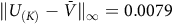 $\Vert U_{(K)} - \bar{V} \Vert_\infty = 0.0079$
. Such an error is inevitable since the value function is an approximation to the satisfaction probability. Meanwhile, a random initialization
$\Vert U_{(K)} - \bar{V} \Vert_\infty = 0.0079$
. Such an error is inevitable since the value function is an approximation to the satisfaction probability. Meanwhile, a random initialization
 $U_0 \sim [0,1]^{m+n}$
or a nonzero constant
$U_0 \sim [0,1]^{m+n}$
or a nonzero constant
 $U_0 = c \mathbb{I}$
with
$U_0 = c \mathbb{I}$
with
 $c\in (0,1)$
violates the condition, and
$c\in (0,1)$
violates the condition, and
 $U_{(K)}$
converges to a solution not satisfying the condition. We obtain significantly larger errors
$U_{(K)}$
converges to a solution not satisfying the condition. We obtain significantly larger errors
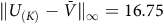 $\Vert U_{(K)} - \bar{V} \Vert_\infty = 16.75$
and
$\Vert U_{(K)} - \bar{V} \Vert_\infty = 16.75$
and
 $3.238$
, respectively. In these cases, the solution does not coincide with the value function of the Bellman equation.
$3.238$
, respectively. In these cases, the solution does not coincide with the value function of the Bellman equation.
Figure 4 shows, the change of approximate value function
 $U_{(k)}$
for all four states
$U_{(k)}$
for all four states
 $\neg B_R$
inside one rejecting BSCCs during updates, given
$\neg B_R$
inside one rejecting BSCCs during updates, given
 $U_0 \sim [0,1]^{m+n}$
. For the case when
$U_0 \sim [0,1]^{m+n}$
. For the case when
 $U_0=\mathbb{O}$
and
$U_0=\mathbb{O}$
and
 $U_0=0.1\mathbb{I}$
, the approximate value function stays at 0 and 1, respectively. Since the Bellman update
$U_0=0.1\mathbb{I}$
, the approximate value function stays at 0 and 1, respectively. Since the Bellman update
 $$U_{(k + 1)}^{\neg {B_R}} = {P_{\pi, \neg {B_R} \to \neg {B_R}}}U_{(k)}^{\neg {B_R}},$$
does not involve discounting within a rejecting BSCC. The approximate value function either converges to the same nonzero constant for all states inside one BSCC or remains unchanged. Given an ill-posed initial condition, this constant differs from the value function, demonstrating that the solution is incorrect when the condition in Theorem 1 does not hold.

Figure 4. Given  $U_0 \sim [0,1]^{m+n}$
, the change of approximate value function
$U_0 \sim [0,1]^{m+n}$
, the change of approximate value function  $U_{(k)}$
for all four states
$U_{(k)}$
for all four states  $s_1,s_2,s_3$
and
$s_1,s_2,s_3$
and  $s_4$
inside one rejecting BSCCs during updates. Since the Bellman update does not involve discounting within a rejecting BSCC, the approximate value function converges to the same nonzero constant for all states inside the BSCC. This constant differs from the value function, demonstrating that the solution is incorrect when the condition in Theorem 1 does not hold.
$s_4$
inside one rejecting BSCCs during updates. Since the Bellman update does not involve discounting within a rejecting BSCC, the approximate value function converges to the same nonzero constant for all states inside the BSCC. This constant differs from the value function, demonstrating that the solution is incorrect when the condition in Theorem 1 does not hold.
Remark 2. The solution
 $U_{(k)}$
found by dynamic programming update is uniquely determined by the initial condition
$U_{(k)}$
found by dynamic programming update is uniquely determined by the initial condition
 $U_0$
. One can show this using a similar procedure in (Xuan and Wang Reference Xuan and Wang2024) with additional convergence analysis of solutions inside rejecting BSCCs. The convergence is shown in Figure 4. However, the fact that the Bellman equation is uniquely determined by the initial condition
$U_0$
. One can show this using a similar procedure in (Xuan and Wang Reference Xuan and Wang2024) with additional convergence analysis of solutions inside rejecting BSCCs. The convergence is shown in Figure 4. However, the fact that the Bellman equation is uniquely determined by the initial condition
 $U_0$
does not mean that it has a unique solution.
$U_0$
does not mean that it has a unique solution.
Validating the uniqueness condition for neural network approximations
We extend the case study to value estimation with neural network function approximation, which is widely used in modern RL for temporal-logic planning. Our aim is to demonstrate that, when
 ${\rm\gamma}=1$
, the uniqueness condition in Theorem 1 is typically violated by neural network generalization. We therefore organize the experiments around three guiding questions: (i) what occurs under standard practice without special handling; (ii) If we mimic the tabular initialization that preserves zeros on rejecting BSCCs, does a neural network keep them at zero? and (iii) whether enforcing the uniqueness condition leads to a more accurate solution. These questions correspond to the following setups.
${\rm\gamma}=1$
, the uniqueness condition in Theorem 1 is typically violated by neural network generalization. We therefore organize the experiments around three guiding questions: (i) what occurs under standard practice without special handling; (ii) If we mimic the tabular initialization that preserves zeros on rejecting BSCCs, does a neural network keep them at zero? and (iii) whether enforcing the uniqueness condition leads to a more accurate solution. These questions correspond to the following setups.
-
Baseline: We train on all states with standard random initialization. This represents the most common practice in RL. It highlights that without any special treatment, the estimated values of rejecting BSCC states deviate from the true solution, yielding large errors.
-
Init0: train on all states with the output bias initialized so that
$V_\theta(s)= 0$
at the start. This shows that even if value function estimations for rejecting BSCCs start at zero, generalization during training makes their values drift away from zero. -
Subset: train only on states that are not in rejecting BSCCs. Rejecting BSCC states
$\neg B_R$
are excluded from both the model’s input and its output. This represents the ideal case when our condition holds, even though current work using neural networks does not achieve this.


We approximate the value function with a neural network
 $V_\theta$
implemented in Python/PyTorch with double precision. After k optimization steps the parameters are
$V_\theta$
implemented in Python/PyTorch with double precision. After k optimization steps the parameters are
 $\theta_k$
and the output at state s is
$\theta_k$
and the output at state s is
 $V_{\theta_k}(s)$
. All losses and metrics are functions of
$V_{\theta_k}(s)$
. All losses and metrics are functions of
 $\theta_k$
. The neural network
$\theta_k$
. The neural network
 $V_\theta$
maps a discrete state index to a trainable 16-dimensional embedding, followed by two hidden layers of width 64 with LeakyReLU activations
$V_\theta$
maps a discrete state index to a trainable 16-dimensional embedding, followed by two hidden layers of width 64 with LeakyReLU activations
 $\phi(x)=\max\{x,-0.01x\}$
and a linear output head. Training minimizes the mean squared Bellman error on the training set
$\phi(x)=\max\{x,-0.01x\}$
and a linear output head. Training minimizes the mean squared Bellman error on the training set
 $S_{{\rm train}}$
,
$S_{{\rm train}}$
,
 $${\cal L}({\theta _k}) = {1 \over {|{S_{{\rm{train}}}}|}}\sum\limits_{s\,\in\, {S_{{\rm{train}}}}} \Big( {V_{{\theta _k}}}(s) - R(s) - \Gamma (s)\sum\limits_{s'} P (s,s'){\mkern 1mu} {V_{{\theta _k}}}(s'){\Big)^2},$$
using AdamW with learning rate
 $10^{-4}$
. In Baseline and Init0 we use the full state space
$10^{-4}$
. In Baseline and Init0 we use the full state space
 $S_{{\rm train}}=S$
(with Init0 initializing the output bias so that
$S_{{\rm train}}=S$
(with Init0 initializing the output bias so that
 $V_{\theta_0}(s)\approx 0$
). In Subset we train only on states outside rejecting BSCCs,
$V_{\theta_0}(s)\approx 0$
). In Subset we train only on states outside rejecting BSCCs,
 $S_{{\rm train}}=S\setminus \neg B_R$
, and whenever a Bellman target requires a successor
$S_{{\rm train}}=S\setminus \neg B_R$
, and whenever a Bellman target requires a successor
 $s'\in\neg B_R$
we substitute 0 for its value.
$s'\in\neg B_R$
we substitute 0 for its value.
Accuracy and the uniqueness condition are evaluated by mean squared errors (MSE) with respect to the previously computed true value function
 $\bar V$
, the solution of the Bellman equation with
$\bar V$
, the solution of the Bellman equation with
 ${\rm\gamma}=1$
and
${\rm\gamma}=1$
and
 ${\rm\gamma}_B=0.999$
. We report the mean squared error over the evaluation set
${\rm\gamma}_B=0.999$
. We report the mean squared error over the evaluation set
 $${\rm{MS}}{{\rm{E}}_S}({\theta _k}) = {1 \over {|{S_{eval}}|}}\sum\limits_{s\,\in\, {S_{eval}}} ( {V_{{\theta _k}}}(s) - \bar V(s){)^2},$$
and the mean squared error on rejecting BSCC states
 $${\rm{MS}}{{\rm{E}}_{\neg {B_R}}}({\theta _k}) = {1 \over {|\neg {B_R}|}}\sum\limits_{s\,\in\, \neg {B_R}} ( {V_{{\theta _k}}}(s) - \bar V(s){)^2},$$
where
 $S_{eval}=S$
for the setup Init0 and Baseline and
$S_{eval}=S$
for the setup Init0 and Baseline and
 $S_{eval}=S\backslash \neg B_R$
for the setup Subset. We use MSE because it measures errors across all states in S and
$S_{eval}=S\backslash \neg B_R$
for the setup Subset. We use MSE because it measures errors across all states in S and
 $\neg B_R$
, whereas
$\neg B_R$
, whereas
 $L_\infty$
used in the tabular case reflects only the single worst state.
$L_\infty$
used in the tabular case reflects only the single worst state.
The experiments show that neural networks break the uniqueness condition. Training converges in all three setups, as shown in Figure 5. In Figure 5(a) the loss
 $\mathcal{L}(\theta_k)$
decreases in every setup and, after
$\mathcal{L}(\theta_k)$
decreases in every setup and, after
 $k\geq 8\times10^{4}$
, remains below
$k\geq 8\times10^{4}$
, remains below
 $10^{-5}$
. Figure 5(b) shows that
$10^{-5}$
. Figure 5(b) shows that
 ${\rm MSE}_{\neg B_R}(\theta_k)$
on the evaluation set changes only slightly once
${\rm MSE}_{\neg B_R}(\theta_k)$
on the evaluation set changes only slightly once
 ${\mathcal{L}}(\theta_k)$
has stabilized. Throughout training, Subset yields a distinctly smaller
${\mathcal{L}}(\theta_k)$
has stabilized. Throughout training, Subset yields a distinctly smaller
 ${\rm MSE}_{\neg B_R}(\theta_k)$
than Baseline and Init0 because, when computing Bellman targets, transitions into
${\rm MSE}_{\neg B_R}(\theta_k)$
than Baseline and Init0 because, when computing Bellman targets, transitions into
 $\neg B_R$
use a fixed value 0. Therefore, errors on
$\neg B_R$
use a fixed value 0. Therefore, errors on
 $\neg B_R$
do not propagate to the rest of the state space. In contrast, Figure 6 shows that the uniqueness condition is violated in both Baseline and Init0:
$\neg B_R$
do not propagate to the rest of the state space. In contrast, Figure 6 shows that the uniqueness condition is violated in both Baseline and Init0:
 ${\rm MSE}_{\neg B_R}(\theta_k)$
converges to a nonzero level, and although Init0 starts near zero by construction, its error quickly rises to a nonzero plateau due to training-induced generalization.
${\rm MSE}_{\neg B_R}(\theta_k)$
converges to a nonzero level, and although Init0 starts near zero by construction, its error quickly rises to a nonzero plateau due to training-induced generalization.

Figure 5. Neural network value approximation under three setups: Subset (train only on
 $S\backslash \neg B_R$
, excluding
$S\backslash \neg B_R$
, excluding
 $\neg B_R$
from inputs/outputs), Baseline (train on all states with standard initialization), and Init0 (train on all states with zero-bias initialization so
$\neg B_R$
from inputs/outputs), Baseline (train on all states with standard initialization), and Init0 (train on all states with zero-bias initialization so
 $V_\theta(s)\approx 0$
at
$V_\theta(s)\approx 0$
at
 $k{=}0$
). (a) Training loss
$k{=}0$
). (a) Training loss
 $\mathcal{L}(\theta_k)$
, i.e., the mean squared Bellman residual on
$\mathcal{L}(\theta_k)$
, i.e., the mean squared Bellman residual on
 $S_{{\rm train}}$
. (b) Value error
$S_{{\rm train}}$
. (b) Value error
 ${\rm MSE}_{\mathcal{S}}(\theta_k)$
on the evaluation set. Empirically, for all setups, the training loss drops and, after
${\rm MSE}_{\mathcal{S}}(\theta_k)$
on the evaluation set. Empirically, for all setups, the training loss drops and, after
 $k\geq 8\times 10^{4}$
, stabilizes below
$k\geq 8\times 10^{4}$
, stabilizes below
 $10^{-5}$
, while the value error changes only marginally thereafter. The Subset setup yields substantially smaller value error than Baseline and Init0.
$10^{-5}$
, while the value error changes only marginally thereafter. The Subset setup yields substantially smaller value error than Baseline and Init0.

Figure 6.
 ${\rm MSE}_{\neg B_R}(\theta_k)$
on rejecting BSCCs. The error in both Baseline and Init0 converges to an incorrect, nonzero level, indicating the neural network outputs on
${\rm MSE}_{\neg B_R}(\theta_k)$
on rejecting BSCCs. The error in both Baseline and Init0 converges to an incorrect, nonzero level, indicating the neural network outputs on
 $\neg B_R$
violate the uniqueness condition in Theorem 1. Although Init0 starts near zero by construction, its error quickly rises to a nonzero plateau due to generalization during training.
$\neg B_R$
violate the uniqueness condition in Theorem 1. Although Init0 starts near zero by construction, its error quickly rises to a nonzero plateau due to generalization during training.
Conclusion
This work uncovers a challenge when using surrogate rewards with two discount factors for LTL objectives, which has been unfortunately overlooked by many previous works. Specifically, we show setting one of the discount factors to one can cause the Bellman equation to have multiple solutions, hindering the derivation of the value function. We discuss the uniqueness of the solution for the Bellman Equation with two discount factors and propose a condition to identify the value function from the multiple solutions. Finally, our case study demonstrates that correctly solving the Bellman equation requires this uniqueness condition, while in practice this condition can be violated in deep RL for LTL objectives.
Data availability statement
The code for the Markov chain, dynamic programming, and numerical validations can be found in our lab’s GitHub repository: https://github.com/SmartAutonomyLab/Unique-Solution-of-the-Bellman-Equation-for-LTL.
Author contributions
Zetong Xuan, Alper Bozkurt, Miroslav Pajic, and Yu Wang contributed to the conception and development of the theoretical framework. Zetong Xuan conducted the experiments. All authors participated in interpreting the results, revising the manuscript for important intellectual content, and approving the final version for publication. All authors agree to be accountable for the integrity and accuracy of the work.
Financial support
This work is sponsored in part by the AFOSR under the award number FA9550-19-1-0169, and by the NSF under NAIAD Award 2332744 as well as the National AI Institute for Edge Computing Leveraging Next Generation Wireless Networks, Grant CNS-2112562.
Competing interests
None.
Ethical standards
The research meets all ethical guidelines, including adherence to the legal requirements of the study country.


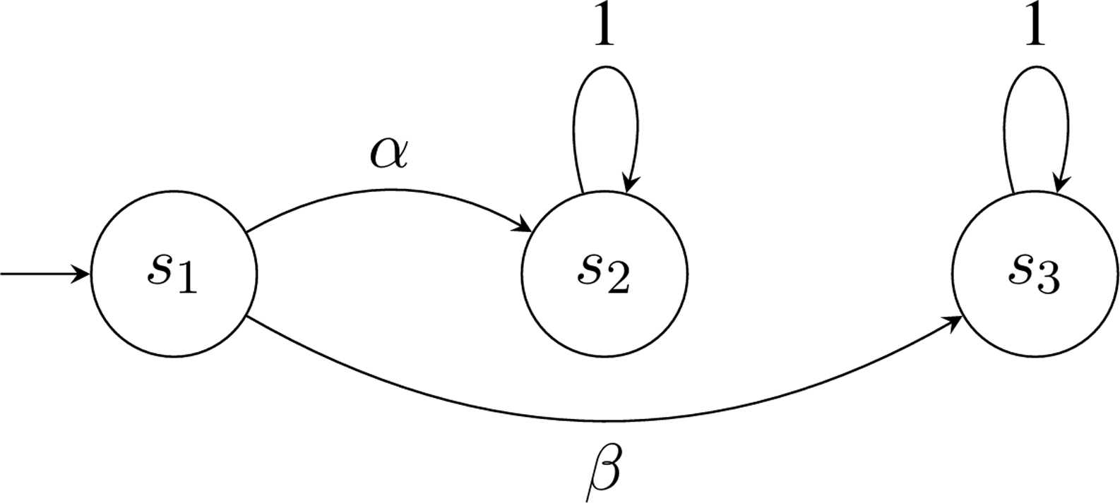

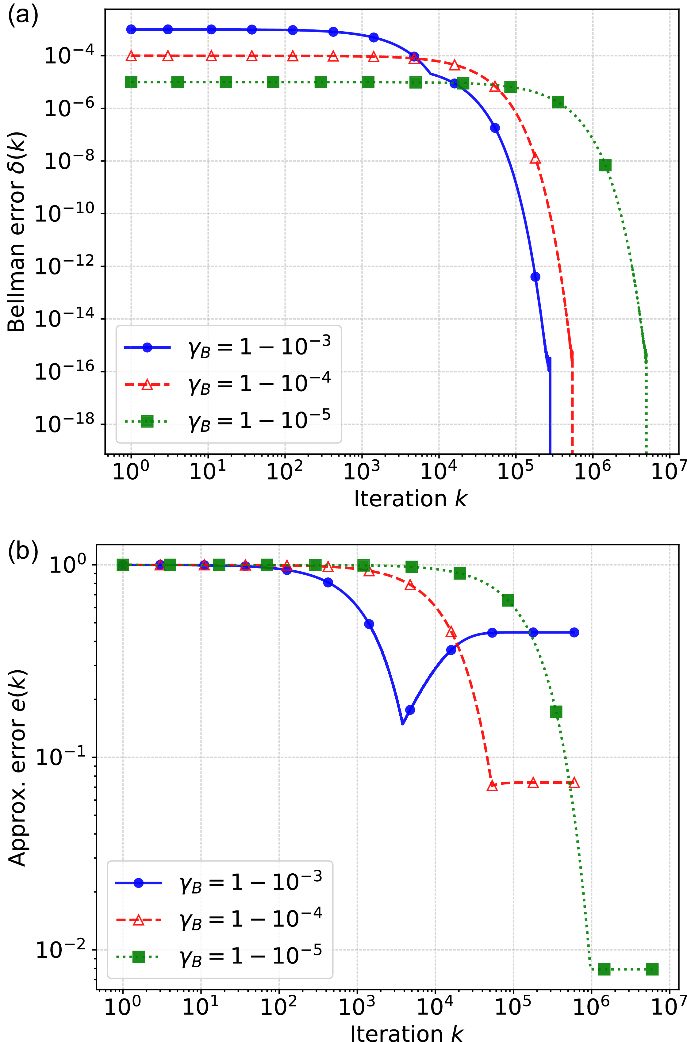


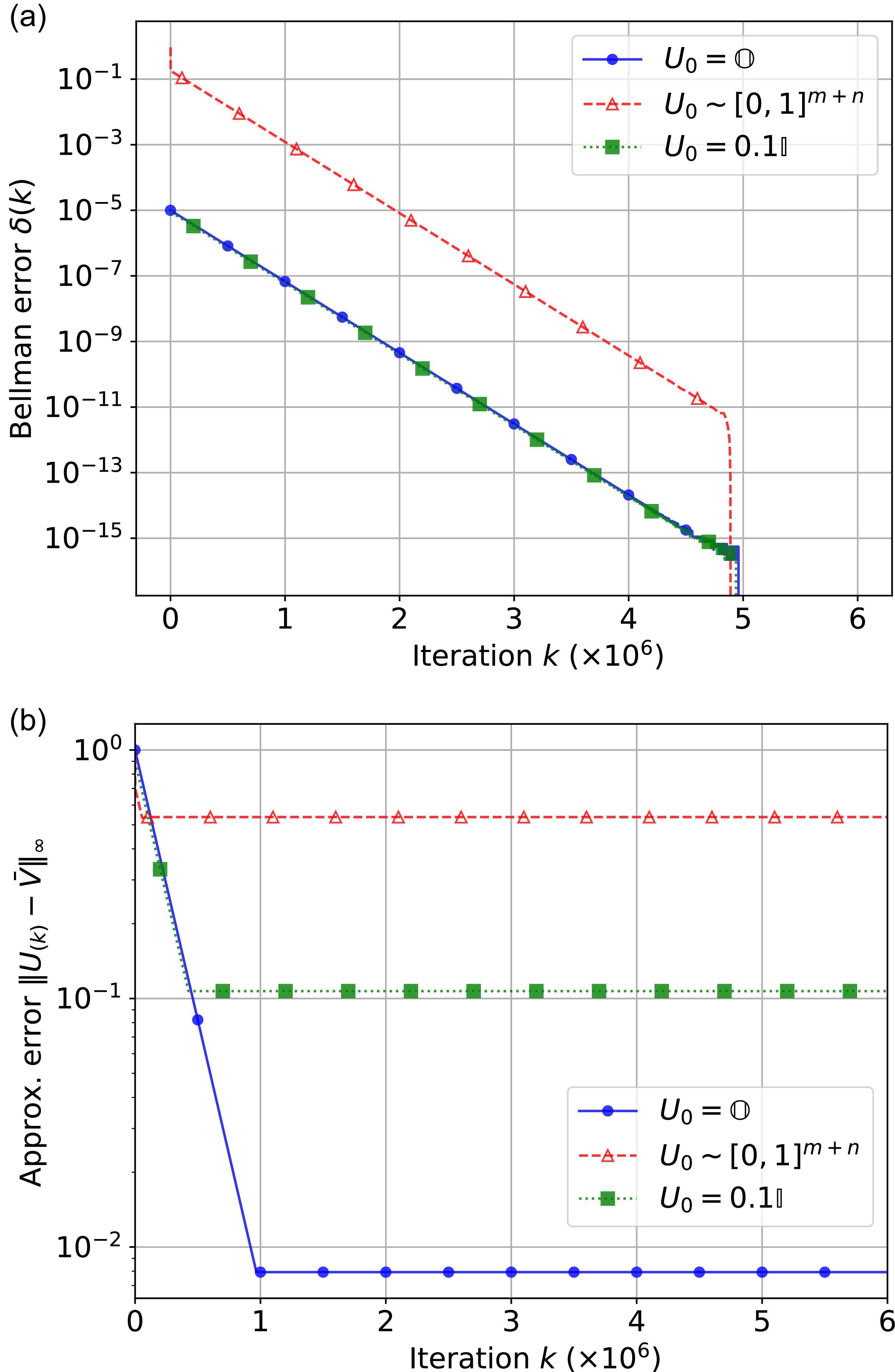


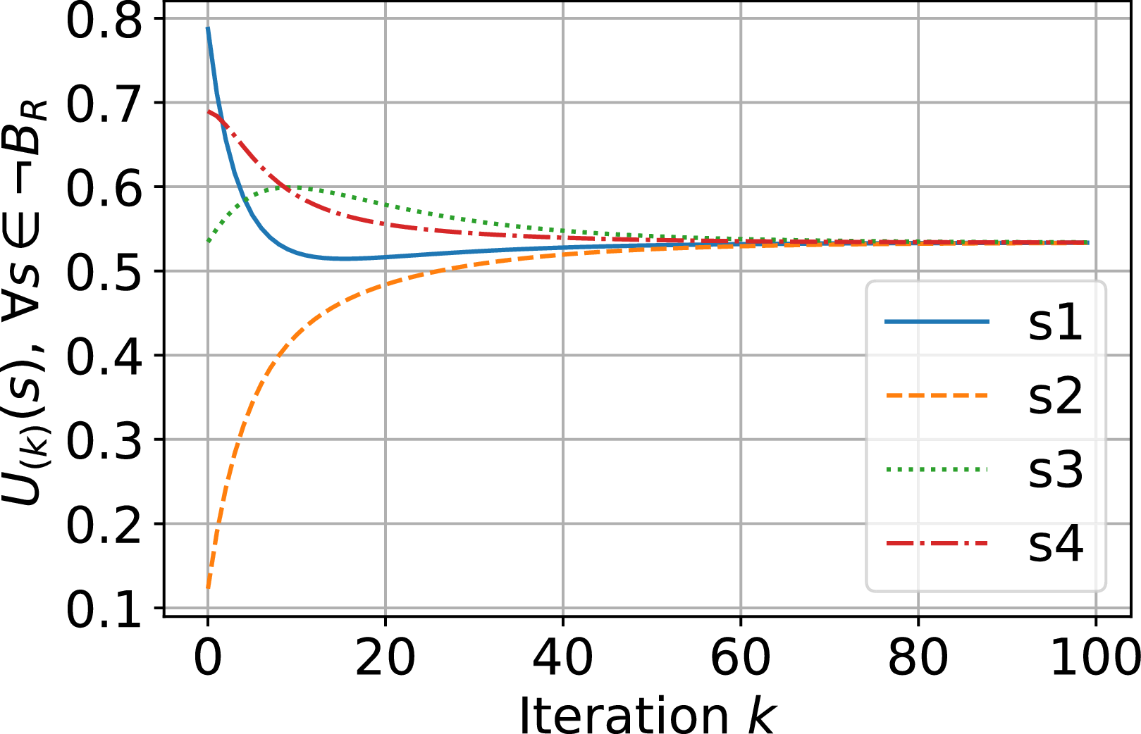


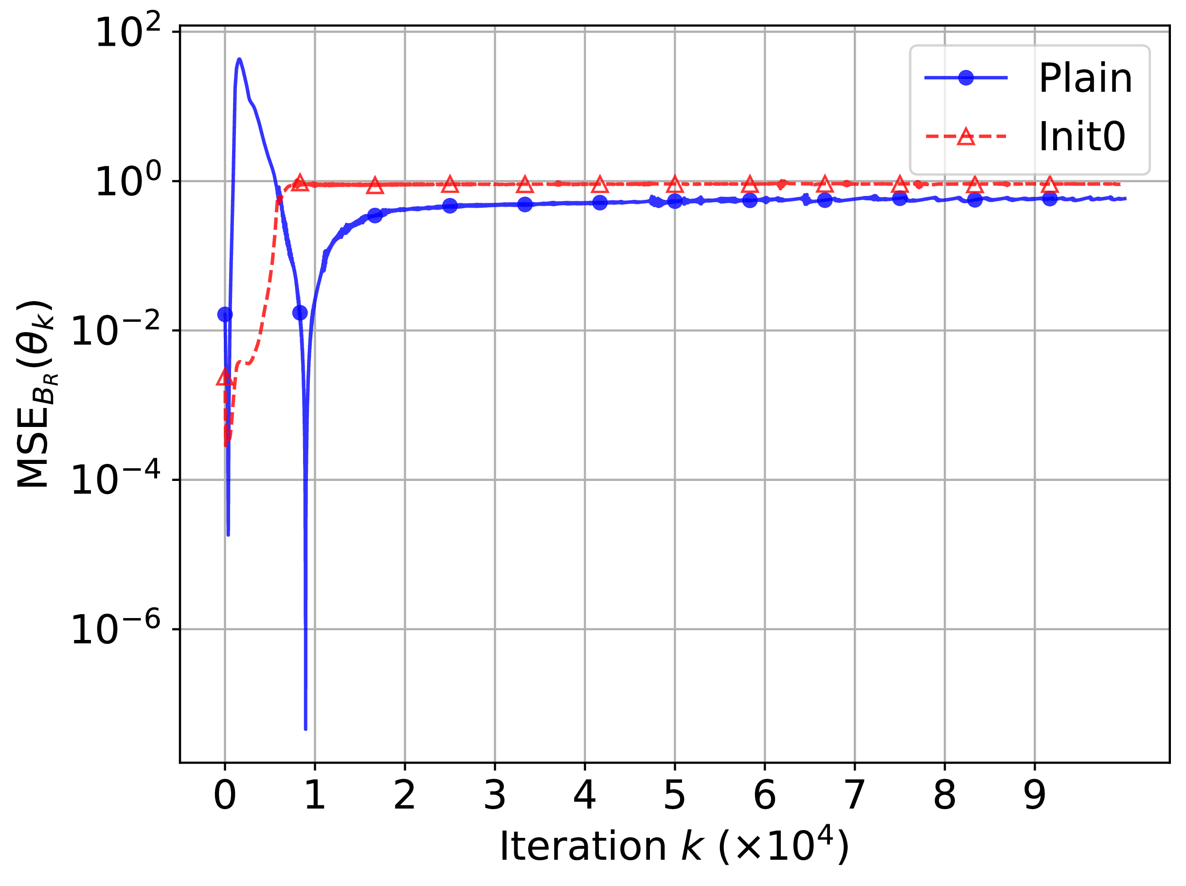


 Open access
Comments
No accompanying comment.