


1. Introduction
Particle-laden jets often arise in nature in the form of volcanic plumes (Kieffer & Sturtevant Reference Kieffer and Sturtevant1984; Viggiano et al. Reference Viggiano, Gish, Solovitz and Cal2024) and hydrothermal eruptions (McKibbin, Smith & Fullard Reference McKibbin, Smith and Fullard2009). Likewise, particle-laden jet flows can be found in numerous advanced engineering applications such as cold spray manufacturing (Alkhimov et al. Reference Alkhimov, Papyrin, Kosarev, Nesterovich and Shushpanov1994; Herman & Sampath Reference Herman and Sampath1996), metallurgy (Wei et al. Reference Wei, Zhu, Yang, Hu, Yang and Chen2020), nanothermite combustion for propulsion applications (Apperson et al. Reference Apperson, Bezmelnitsyn, Thiruvengadathan, Gangopadhyay, Gangopadhyay, Balas, Anderson and Nicolich2009), targeted drug delivery (Arora et al. Reference Arora, Hakim, Baxter, Rathnasingham, Srinivasan, Fletcher and Mitragotri2007; Kleinstreuer, Zhang & Donohue Reference Kleinstreuer, Zhang and Donohue2008), transmission of diseases through sneezing and coughing (Mittal, Ni & Seo Reference Mittal, Ni and Seo2020; Bourouiba Reference Bourouiba2021) and particle entrainment in jets used in the final approach of lander modules to the surface of extraterrestrial bodies (Jaffe Reference Jaffe1971; Sengupta et al. Reference Sengupta, Kulleck, Sell, Van Norman, Mehta and Pokora2009). Regardless of the nature of these jets, the particle distribution in such flows has been a source of long-standing questions that have motivated numerous research campaigns in this field. To fully grasp particle dispersion in a jet, three main aspects of particle–fluid interaction require understanding. These are discussed in the following subsections.
1.1. Particle clustering
Generally, in turbulent flows, particles are known to be ejected from vortices based on their inertia, and cluster where vorticity is low (Squires & Eaton Reference Squires and Eaton1991) or in locations where their net acceleration is zero (Goto & Vassilicos Reference Goto and Vassilicos2008). The mechanism of particle clustering in low vorticity (high strain-rate) regions due to the centrifugal force exerted on the particles by coherent turbulent structures is called preferential concentration (PC), and it is the most widely accepted explanation for turbulence-induced particle clustering. Furthermore, it has been reported that, in jet flows, particles preferentially gather in the regions with a local streamwise velocity higher than the mean velocity (Li et al. Reference Li, Fan, Luo and Cen2011). Moreover, in general, compressibility and shear play a significant role in the particle dynamics, where, apart from PC (which is still blamed for clustering Zhang et al. Reference Zhang, Liu, Ma and Xiao2016), particle clustering intensifies with the increase in compressibility (Pérez-Munuzuri Reference Pérez-Munuzuri2015). This is particularly important for high-speed jet flows which involve significant compressibility and shear.
Regardless of the particle clustering mechanism, clustering is driven by turbulent eddies and the particles’ response to these eddies based on their inertia. In homogeneous isotropic turbulence (HIT), tracer particles with virtually no inertia can closely follow the coherent turbulent structures (Bec et al. Reference Bec, Biferale, Cencini, Lanotte and Toschi2006). Therefore, tracer-like particles are often used in experimental techniques such as particle image velocimetry for measuring flow parameters (Adrian Reference Adrian1984). On the contrary, heavy particles tend to be ballistic, and thus their motion is weakly influenced by local eddies (Balachandar & Eaton Reference Balachandar and Eaton2010). A dimensionless parameter called the Stokes number ( ${\textit{St}}$
) is typically used to characterise the inertia-based correlation between the particles and turbulence, as discussed later in this section.
${\textit{St}}$
) is typically used to characterise the inertia-based correlation between the particles and turbulence, as discussed later in this section.
1.2. Particle transport
In the context of jets, apart from clustering, particle inertia also determines particle trajectories as the jet develops (Casciola et al. Reference Casciola, Gualtieri, Picano, Sardina and Troiani2010); whether particles travel within the jet or are dispersed away from the jet centreline. Predicting particle trajectories is critical for numerous applications. For example, in cold spray advanced manufacturing techniques, the goal is to keep the particle inside the high-speed jet, as particle dispersion drops coating efficiency (Meyer, Yin & Lupoi Reference Meyer, Yin and Lupoi2017). Favourably, the presence of particles narrows the spreading of the jet and enhances the centreline velocity as particle motion is governed by the kinetic energy of the gas (Hetsroni & Sokolov Reference Hetsroni and Sokolov1971). This effect is desirable for cold sprays. On the other hand, in combustion applications, efficient combustion relies on higher radial dispersion of the fuel droplets (Basu et al. Reference Basu, Agarwal, Mukhopadhyay and Patel2018), considering that these droplets can coalesce, which can greatly limit their dispersion by increasing the droplet size (Gopireddy, Humza & Gutheil Reference Gopireddy, Humza and Gutheil2012). Hence, to manage the radial dispersion of particles based on the application, there is a pressing need to delineate the mechanisms that lead to this dispersion.
For estimating the dispersion of particles inside a jet, the Stokes number ( ${\textit{St}}$
) (Crowe, Gore & Troutt Reference Crowe, Gore and Troutt1985) has been extensively used, which is the ratio of particle momentum response time (
${\textit{St}}$
) (Crowe, Gore & Troutt Reference Crowe, Gore and Troutt1985) has been extensively used, which is the ratio of particle momentum response time ( $\tau _{\!p}$
) to a characteristic turbulent time scale (
$\tau _{\!p}$
) to a characteristic turbulent time scale ( $\tau$
). In jet flows, it is reported that the integral/convective time scale (
$\tau$
). In jet flows, it is reported that the integral/convective time scale ( $\tau _c$
) of the jet governs particle dispersion (Hardalupas, Taylor & Whitelaw Reference Hardalupas, Taylor and Whitelaw1989; Picano et al. Reference Picano, Sardina, Gualtieri and Casciola2010). Hence,
$\tau _c$
) of the jet governs particle dispersion (Hardalupas, Taylor & Whitelaw Reference Hardalupas, Taylor and Whitelaw1989; Picano et al. Reference Picano, Sardina, Gualtieri and Casciola2010). Hence, ${\textit{St}}$
can be written as
${\textit{St}}$
can be written as
 \begin{equation} St = \frac {\tau _{\!p}}{\tau _c} = \frac { \dfrac {\rho _{\!p}\ d_{\!p}^2} {18 \rho _g \nu _g}} {\dfrac {r_{1/2}} {u_c}} .\end{equation}
In (1.1), $\rho$
,
$\rho$
, $\nu$
,
$\nu$
, $u$
,
$u$
, $d$
and
$d$
and $r_{1/2}$
represent density, kinematic viscosity, flow velocity, diameter and jet half-width, respectively. The subscripts
$r_{1/2}$
represent density, kinematic viscosity, flow velocity, diameter and jet half-width, respectively. The subscripts $c$
,
$c$
, $g$
and
$g$
and $p$
denote jet convective/centreline, gas and particle parameters. The value of
$p$
denote jet convective/centreline, gas and particle parameters. The value of $\tau _c$
increases with the axial distance from the jet inlet due to the concurrent effect of increasing
$\tau _c$
increases with the axial distance from the jet inlet due to the concurrent effect of increasing $r_{1/2}$
and decreasing
$r_{1/2}$
and decreasing $u_c$
. Hence, the local particle
$u_c$
. Hence, the local particle ${\textit{St}}$
decreases quadratically along the jet centreline (Picano et al. Reference Picano, Sardina, Gualtieri and Casciola2011). Note that
${\textit{St}}$
decreases quadratically along the jet centreline (Picano et al. Reference Picano, Sardina, Gualtieri and Casciola2011). Note that $\tau _c$
is analogous to the integral time scale (
$\tau _c$
is analogous to the integral time scale ( $\tau _l$
) and at the inlet it is given as
$\tau _l$
) and at the inlet it is given as $\tau _l = r_{\!j} / u_{\!j}$
, where
$\tau _l = r_{\!j} / u_{\!j}$
, where $r_{\!j}$
and
$r_{\!j}$
and $u_{\!j}$
are the jet radius and inlet velocity, respectively. Thus, the initial integral length scale is
$u_{\!j}$
are the jet radius and inlet velocity, respectively. Thus, the initial integral length scale is $L = r_{\!j}$
.
$L = r_{\!j}$
.
The dispersion rate of particles with ${\textit{St}} \ll 1$
is similar to the turbulence dispersion, which causes particles to spread evenly within the jet: particles with
${\textit{St}} \ll 1$
is similar to the turbulence dispersion, which causes particles to spread evenly within the jet: particles with ${\textit{St}} \gg 1$
travel along the jet centreline with minimum radial dispersion; particles with
${\textit{St}} \gg 1$
travel along the jet centreline with minimum radial dispersion; particles with ${\textit{St}} \approx 1$
depict higher dispersion than the turbulent eddies due to the local vortex-based centrifugal force exerted on them, and they can be completely ejected out of the jet (Chung & Troutt Reference Chung and Troutt1988). These three dispersion mechanisms are termed the vortex, inertial and centrifugal mechanisms (Uthuppan et al. Reference Uthuppan, Aggarwal, Grinstein and Kailasanath1994). Furthermore, since
${\textit{St}} \approx 1$
depict higher dispersion than the turbulent eddies due to the local vortex-based centrifugal force exerted on them, and they can be completely ejected out of the jet (Chung & Troutt Reference Chung and Troutt1988). These three dispersion mechanisms are termed the vortex, inertial and centrifugal mechanisms (Uthuppan et al. Reference Uthuppan, Aggarwal, Grinstein and Kailasanath1994). Furthermore, since ${\textit{St}}$
decreases axially, a higher local concentration is observed in the jet where the local
${\textit{St}}$
decreases axially, a higher local concentration is observed in the jet where the local ${\textit{St}} \approx 1$
(Picano et al. Reference Picano, Sardina, Gualtieri and Casciola2011). But eventually, in the far field, particles start behaving as tracers with respect to the large-scale structures, whereas they are ballistic for small-scale velocity fluctuations (Casciola et al. Reference Casciola, Gualtieri, Picano, Sardina and Troiani2010). Hence, as stated earlier, overall in free-shear flows, the dispersion of particles is driven by large-scale vortex structures generated in these flows (Tang et al. Reference Tang, Wen, Yang, Crowe, Chung and Troutt1992). Even in compressible particle-laden flows, which typically involve a larger number of turbulent scales than incompressible flows (Capecelatro & Wagner Reference Capecelatro and Wagner2024), particle clustering is characterised by the large scales and the corresponding
${\textit{St}} \approx 1$
(Picano et al. Reference Picano, Sardina, Gualtieri and Casciola2011). But eventually, in the far field, particles start behaving as tracers with respect to the large-scale structures, whereas they are ballistic for small-scale velocity fluctuations (Casciola et al. Reference Casciola, Gualtieri, Picano, Sardina and Troiani2010). Hence, as stated earlier, overall in free-shear flows, the dispersion of particles is driven by large-scale vortex structures generated in these flows (Tang et al. Reference Tang, Wen, Yang, Crowe, Chung and Troutt1992). Even in compressible particle-laden flows, which typically involve a larger number of turbulent scales than incompressible flows (Capecelatro & Wagner Reference Capecelatro and Wagner2024), particle clustering is characterised by the large scales and the corresponding ${\textit{St}}$
.
${\textit{St}}$
.
1.3. Particle–turbulence interaction
Although particle transport is governed by the local mean and fluctuating fluid velocity, the presence of particles modulates the local turbulent flow field. The overarching mechanism is that particles act as a medium for augmenting the transport of energy (Liu et al. Reference Liu, Tang, Shen and Dong2017) and momentum (Richter & Sullivan Reference Richter and Sullivan2013) between different regions of the flow. Consequently, as compared with a single-phase jet, particles reduce turbulent intensity by up to $50\,\%$
(Yuu, Ikeda & Umekage Reference Yuu, Ikeda and Umekage1996). This jet modulation is a function of the particle loading density (Levy & Lockwood Reference Levy and Lockwood1981; Tsuji et al. Reference Tsuji, Morikawa, Tanaka, Karimine and Nishida1988),
$50\,\%$
(Yuu, Ikeda & Umekage Reference Yuu, Ikeda and Umekage1996). This jet modulation is a function of the particle loading density (Levy & Lockwood Reference Levy and Lockwood1981; Tsuji et al. Reference Tsuji, Morikawa, Tanaka, Karimine and Nishida1988), ${\textit{St}}$
(Kulick, Fessler & Eaton Reference Kulick, Fessler and Eaton1994), particle-to-fluid density ratio, particle diameter to turbulent eddy diameter ratio and the Reynolds number of the particles (
${\textit{St}}$
(Kulick, Fessler & Eaton Reference Kulick, Fessler and Eaton1994), particle-to-fluid density ratio, particle diameter to turbulent eddy diameter ratio and the Reynolds number of the particles ( ${\textit{Re}}_{\!p}$
) (Yarin & Hetsroni Reference Yarin and Hetsroni1994). Such interaction between the two phases creates a feedback loop, making this a compounding problem. Thus, to complete the scope of this issue, it is essential to comprehend the particle-based modulation of a jet flow.
${\textit{Re}}_{\!p}$
) (Yarin & Hetsroni Reference Yarin and Hetsroni1994). Such interaction between the two phases creates a feedback loop, making this a compounding problem. Thus, to complete the scope of this issue, it is essential to comprehend the particle-based modulation of a jet flow.
In the case of supersonic jet flows, smaller particles have been reported to produce a more pronounced modulation of the jet structure as compared with larger particles (Sommerfeld Reference Sommerfeld1994). This is due to the higher specific surface area (ratio of particle surface area to volume) of the smaller particles, which results in stronger fluid–particle momentum exchange at constant particle loading density (Li et al. Reference Li, Li, Zhang, Li, Wu and Zou2020). Moreover, even at minimal particle loading, particles have been found to move the Mach disk upstream in supersonic jet flows (Patel et al. Reference Patel, Rubio, Shekhtman, Parziale, Rabinovitch, Ni and Capecelatro2024). This effect further enhances with the increase in particle loading (Lewis Jr & Carlson Reference Lewis and Carlson1964; Jarvinen & Draper Reference Jarvinen and Draper1967). Additionally, phenomena such as attenuation of dilatation, turbulent Mach number, turbulent kinetic energy and dissipation increase with the density of the particles (Xia et al. Reference Xia, Shi, Zhang and Chen2016), further making the fluid–particle interaction in compressible flows perplexing. The transfer of gas kinetic energy to particles restricts the gas expansion, which decreases the gas density and dynamic pressure in the direction of the flow (Yu et al. Reference Yu, Yang, Hu and Wang2023). In supersonic jets, particles also weaken the pressure functions radiated by a supersonic jet, by substantially altering the development of turbulent structures (Greska Reference Greska2005). Consequently, the root-mean-square jet axial (radial) velocity drops by $10 \,\%$
(
$10 \,\%$
( $30 \,\%$
), as compared with an unladen jet (Krothapalli et al. Reference Krothapalli, Venkatakrishnan, Lourenco, Greska and Elavarasan2003). This effect is also a function of particle mass loading, such that these pressure fluctuations decrease with the increase in mass loading (Buchta, Shallcross & Capecelatro Reference Buchta, Shallcross and Capecelatro2019).
$30 \,\%$
), as compared with an unladen jet (Krothapalli et al. Reference Krothapalli, Venkatakrishnan, Lourenco, Greska and Elavarasan2003). This effect is also a function of particle mass loading, such that these pressure fluctuations decrease with the increase in mass loading (Buchta, Shallcross & Capecelatro Reference Buchta, Shallcross and Capecelatro2019).
As stated in the discussion above, particle dispersion is primarily credited to the centrifugal force acting on the particles based on particle inertia, even in supersonic flows (Li et al. Reference Li, Li, Shao, Li, Zou and Li2021). Here, PC in the axial direction is attributed to the particle–gas momentum transfer, while radial dispersion is credited to the radial inter-phase velocity difference. Note that, in a jet flow in which the particle velocity is less than the fluid velocity at the inlet, particles keep accelerating after leaving the nozzle, consuming the kinetic energy of the supersonic gas. Since the major component of particle inertia is in the streamwise direction, a question arises: Why do particles start travelling in the radial direction in the first place? It is understood that a jet inherently spreads, creating a radial velocity difference between the inertial particle and the local gas. But the particle–gas axial velocity difference is higher in the streamwise direction (up to four times in the present study), and hence particles should keep travelling within the jet centre. We hypothesise that there must be an organised turbulent motion that pushes particles out of the central region of the jet. Local kinematic and thermodynamic aspects, especially fluid viscosity, have been reported to considerably alter the particle distribution in HIT (Saieed & Hickey Reference Saieed and Hickey2022, Reference Saieed and Hickey2023, Reference Saieed and Hickey2024; Saieed, Rahman & Hickey Reference Saieed, Rahman and Hickey2022). In supersonic jet flows, although the local thermodynamic properties of the fluid will change as the jet evolves, these local thermodynamic properties, particularly the fluid viscosity, are assumed to have a minor effect on particle dispersion. In a supersonic jet flow, the variation in density and fluid compressibility governs the fluid–particle interaction, as discussed earlier in this section. Thus, in this contribution, we probe the dispersion of four particle sizes in a supersonic jet flow using direct numerical simulations (DNS). We aim to investigate the local turbulent eddy-based effects that govern the transition of the particles’ motion from axial to radial downstream of the inlet. In the rest of this article, we discuss the methodology of our numerical experiments along with the model validation in § 2, the obtained results in § 3 and the drawn conclusions are reported in § 5.
2. Methodology
We carried out DNS to simulate a spatially developing, polydispersed particle-laden perfectly expanded (shock-free) (Andrews Jr et al. Reference Andrews, Craidon, Dennard and Vick1964; Hinh, Martinuzzi & Johansen Reference Hinh, Martinuzzi and Johansen2025) supersonic jet flow using an in-house version of an effectively parallelised, open-source, high-order finite difference code, known as Pencil-Code (Brandenburg et al. Reference Brandenburg2020). A sixth-order scheme is used for spatial derivatives, and a third-order Runge–Kutta scheme is employed for time integration. To stabilise our sixth-order spatial scheme, which is inherently unstable with finite difference, a hyperdiffusion term was used. The domain pressure was matched with the inlet pressure of the jet to avoid the formation of large-scale shocks. In other words, the ratio of jet exit to domain pressure is maintained at unity (nozzle pressure ratio, $\mathrm{NPR}= 1$
). These simulations are carried out in a rectangular domain with a periodic boundary condition (BC) in the lateral direction to eliminate wall effects, which are not of interest in the present study. Four particle sizes are considered with two-way coupling using the Lagrangian point-particle tracking scheme, where a tri-linear interpolation method is used for resolving particle trajectories. In this case, the undisturbed local fluid velocity is required to compute the drag force on the particles. However, it is intrinsically unavailable in two-way momentum coupling as particles influence the local flow field (Horwitz & Mani Reference Horwitz and Mani2016, Reference Horwitz and Mani2018). As a result, the Stokes drag on the particles can be underestimated. Thus, the use of the tri-linear interpolation method can be problematic, especially in supersonic flows, and may require a correction to capture the particle trajectories accurately. A metric for estimating the error due to this scheme is the ratio of particle diameter to grid cell length
$\mathrm{NPR}= 1$
). These simulations are carried out in a rectangular domain with a periodic boundary condition (BC) in the lateral direction to eliminate wall effects, which are not of interest in the present study. Four particle sizes are considered with two-way coupling using the Lagrangian point-particle tracking scheme, where a tri-linear interpolation method is used for resolving particle trajectories. In this case, the undisturbed local fluid velocity is required to compute the drag force on the particles. However, it is intrinsically unavailable in two-way momentum coupling as particles influence the local flow field (Horwitz & Mani Reference Horwitz and Mani2016, Reference Horwitz and Mani2018). As a result, the Stokes drag on the particles can be underestimated. Thus, the use of the tri-linear interpolation method can be problematic, especially in supersonic flows, and may require a correction to capture the particle trajectories accurately. A metric for estimating the error due to this scheme is the ratio of particle diameter to grid cell length $d_{\!p} / l_{\textit{cell}}$
. Since our cell length along
$d_{\!p} / l_{\textit{cell}}$
. Since our cell length along $x$
is less than in the
$x$
is less than in the $y$
and
$y$
and $z$
directions (
$z$
directions ( $\Delta x \lt \Delta y = \Delta z$
), we define
$\Delta x \lt \Delta y = \Delta z$
), we define $l_{\textit{cell}} = V_{\textit{cell}}^{1/3}$
, where
$l_{\textit{cell}} = V_{\textit{cell}}^{1/3}$
, where $V_{\textit{cell}} = \Delta x \times \Delta y \times \Delta z$
is the cell volume. Yang et al. (Reference Yang, Li, Liu, Sun, Yang, Wang, Wang and Li2024) found the tri-linear interpolation method to be invalid if
$V_{\textit{cell}} = \Delta x \times \Delta y \times \Delta z$
is the cell volume. Yang et al. (Reference Yang, Li, Liu, Sun, Yang, Wang, Wang and Li2024) found the tri-linear interpolation method to be invalid if $d_{\!p} / l_{\textit{cell}}$
is large (
$d_{\!p} / l_{\textit{cell}}$
is large ( $O(10^0)$
). Moreover, Patel et al. (Reference Patel, Rubio, Shekhtman, Parziale, Rabinovitch, Ni and Capecelatro2024) suggested the use of an optimised two-way momentum coupling approach for larger
$O(10^0)$
). Moreover, Patel et al. (Reference Patel, Rubio, Shekhtman, Parziale, Rabinovitch, Ni and Capecelatro2024) suggested the use of an optimised two-way momentum coupling approach for larger $d_{\!p} / l_{\textit{cell}}$
and shock–particle interaction. However, in our case, the highest
$d_{\!p} / l_{\textit{cell}}$
and shock–particle interaction. However, in our case, the highest $d_{\!p} / l_{\textit{cell}} = 0.18$
, which is fairly small, and our jet is shock free. Hence, we expect the impact of local disturbed fluid velocity on Stokes drag to be minimal.
$d_{\!p} / l_{\textit{cell}} = 0.18$
, which is fairly small, and our jet is shock free. Hence, we expect the impact of local disturbed fluid velocity on Stokes drag to be minimal.
On the other hand, the diameters and initial ${\textit{St}}$
of these particles are presented in table 1. As seen in table 1, we will refer to these particles with increasing diameter as
${\textit{St}}$
of these particles are presented in table 1. As seen in table 1, we will refer to these particles with increasing diameter as $\mathrm{P1}$
,
$\mathrm{P1}$
, $\mathrm{P2}$
,
$\mathrm{P2}$
, $\mathrm{P3}$
and
$\mathrm{P3}$
and $\mathrm{P4}$
, for brevity. The constant density of these particles is
$\mathrm{P4}$
, for brevity. The constant density of these particles is $\rho _{\!p} = 1500$
. In light of our hypothesis, the use of different particle sizes will enable us to probe the local mechanisms that cause particles to start travelling laterally at different downstream locations. For the continuum phase, the gas with a density of
$\rho _{\!p} = 1500$
. In light of our hypothesis, the use of different particle sizes will enable us to probe the local mechanisms that cause particles to start travelling laterally at different downstream locations. For the continuum phase, the gas with a density of $\rho _g = 1$
is simulated with an Eulerian specification. Our DNS consists of three sub-simulations, as discussed in the following subsections.
$\rho _g = 1$
is simulated with an Eulerian specification. Our DNS consists of three sub-simulations, as discussed in the following subsections.
Table 1. Diameters ( $d_{\!p}$
) and Stokes number (
$d_{\!p}$
) and Stokes number ( ${\textit{St}}$
) at the jet inlet, of the four particle species (denoted
${\textit{St}}$
) at the jet inlet, of the four particle species (denoted $\mathrm{P1}$
to
$\mathrm{P1}$
to $\mathrm{P4}$
).
$\mathrm{P4}$
).

2.1. Simulation set-up
2.1.1. Development of HIT
The simulation set-up is depicted in figure 1. Firstly, HIT is generated in a triply periodic box of $9 d_{\!j}$
characteristic length discretised into a
$9 d_{\!j}$
characteristic length discretised into a $256^3$
mesh, where
$256^3$
mesh, where $d_{\!j}$
is the jet diameter. This simulation is conducted without particles and resulted in a Taylor Reynolds number of
$d_{\!j}$
is the jet diameter. This simulation is conducted without particles and resulted in a Taylor Reynolds number of ${\textit{Re}}_\varLambda = \rho _g u_{\textit{rms}} \varLambda / \mu _g = 77$
, where
${\textit{Re}}_\varLambda = \rho _g u_{\textit{rms}} \varLambda / \mu _g = 77$
, where $\varLambda$
,
$\varLambda$
, $u_{\textit{rms}}$
and
$u_{\textit{rms}}$
and $\mu _g$
are the Taylor microscale, fluid root-mean-square velocity and dynamic viscosity, respectively. For HIT development, a solenoidal forcing function is used (Brandenburg Reference Brandenburg2001). This forcing scheme is such that, at any given instance, the random points of energy addition are correlated, but these points vary in time. This simulation is carried out until an equilibrium is established between energy addition and energy dissipation at high wavenumbers (
$\mu _g$
are the Taylor microscale, fluid root-mean-square velocity and dynamic viscosity, respectively. For HIT development, a solenoidal forcing function is used (Brandenburg Reference Brandenburg2001). This forcing scheme is such that, at any given instance, the random points of energy addition are correlated, but these points vary in time. This simulation is carried out until an equilibrium is established between energy addition and energy dissipation at high wavenumbers ( $k$
). This is determined by the fact that the temporal evolution of turbulence statistics such as turbulent kinetic energy (
$k$
). This is determined by the fact that the temporal evolution of turbulence statistics such as turbulent kinetic energy ( $\mathrm{TKE}$
) starts fluctuating about a steady mean value. Note that, regardless of the forcing scheme used (linear (Rosales & Meneveau Reference Rosales and Meneveau2005; Bassenne et al. Reference Bassenne, Urzay, Park and Moin2016) or spectral (Overholt & Pope Reference Overholt and Pope1998)), turbulence statistics, especially
$\mathrm{TKE}$
) starts fluctuating about a steady mean value. Note that, regardless of the forcing scheme used (linear (Rosales & Meneveau Reference Rosales and Meneveau2005; Bassenne et al. Reference Bassenne, Urzay, Park and Moin2016) or spectral (Overholt & Pope Reference Overholt and Pope1998)), turbulence statistics, especially $\mathrm{TKE}$
, depict noticeable fluctuations about a mean value even after the aforementioned equilibrium is established. Since these fluctuations eventually oscillate about a constant mean value, we consider the HIT to be fully developed. This simulation is conducted for approximately
$\mathrm{TKE}$
, depict noticeable fluctuations about a mean value even after the aforementioned equilibrium is established. Since these fluctuations eventually oscillate about a constant mean value, we consider the HIT to be fully developed. This simulation is conducted for approximately $200$
integral time scales (
$200$
integral time scales ( $\tau _l = r_{\!j} / u_{\!j}$
) computed at the inlet of the jet.
$\tau _l = r_{\!j} / u_{\!j}$
) computed at the inlet of the jet.

Figure 1. Simulation set-up depicting three sub-simulations.
2.1.2. Jet development
Once the HIT is fully developed, three-dimensional (3-D) snapshots of the mean velocity field from the HIT simulation are cyclically introduced at the inlet of a rectangular domain with dimensions $14 d_{\!j} \times 9 d_{\!j} \times 9 d_{\!j}$
. This domain is meshed into
$14 d_{\!j} \times 9 d_{\!j} \times 9 d_{\!j}$
. This domain is meshed into $512 \times 256 \times 256$
cells in the
$512 \times 256 \times 256$
cells in the $x$
,
$x$
, $y$
and
$y$
and $z$
directions. This resulted in grid cells that are longer in the lateral direction, however, all cells in the domain have the same dimensions. The streamwise mesh has more grid points compared with the lateral directions, as our domain is longer in the axial direction. At the inlet of the jet, a top-hat mean flow profile is assumed. This mean flow is superimposed by the turbulence fluctuations generated by the HIT simulation. The 3-D HIT snapshots of the turbulence fluctuations are convected into the domain, which ensures realistic turbulence characteristics within the compressible jet. The pressure at the inlet is set equal to the domain pressure to get a perfectly expanded jet, thus minimising any shocks or large expansion waves. This was done to avoid shock formation, as the interaction of particles with a shock wave will further complicate our model, and it is not in the scope of this analysis.
$z$
directions. This resulted in grid cells that are longer in the lateral direction, however, all cells in the domain have the same dimensions. The streamwise mesh has more grid points compared with the lateral directions, as our domain is longer in the axial direction. At the inlet of the jet, a top-hat mean flow profile is assumed. This mean flow is superimposed by the turbulence fluctuations generated by the HIT simulation. The 3-D HIT snapshots of the turbulence fluctuations are convected into the domain, which ensures realistic turbulence characteristics within the compressible jet. The pressure at the inlet is set equal to the domain pressure to get a perfectly expanded jet, thus minimising any shocks or large expansion waves. This was done to avoid shock formation, as the interaction of particles with a shock wave will further complicate our model, and it is not in the scope of this analysis.
At the inlet and outlet of this domain, inflow and outflow BCs are imposed, respectively. The fluid is allowed to enter the domain only through the jet inlet with a diameter $d_{\!j} = 1$
, and the rest of the inlet is modelled as a wall. The inlet and outlet boundaries suffered from spurious reflections, however, these reflections at the inlet (Lodato, Domingo & Vervisch Reference Lodato, Domingo and Vervisch2008) and outlet (Poinsot & Lelef Reference Poinsot and Lelef1992) are attenuated with a Navier–Stokes Characteristic Boundary Condition.
$d_{\!j} = 1$
, and the rest of the inlet is modelled as a wall. The inlet and outlet boundaries suffered from spurious reflections, however, these reflections at the inlet (Lodato, Domingo & Vervisch Reference Lodato, Domingo and Vervisch2008) and outlet (Poinsot & Lelef Reference Poinsot and Lelef1992) are attenuated with a Navier–Stokes Characteristic Boundary Condition.
A periodic BC is prescribed in the two lateral directions ( $y$
and
$y$
and $z$
). This is done to deal with a limitation of Pencil-Code; where if outflow BC is imposed on the
$z$
). This is done to deal with a limitation of Pencil-Code; where if outflow BC is imposed on the $y$
and
$y$
and $z$
boundaries, the reflections from the edges between these boundaries result in discontinuities. This simulation is run for roughly
$z$
boundaries, the reflections from the edges between these boundaries result in discontinuities. This simulation is run for roughly $7$
flow through times (FTT), such that the initial transience caused by the jet development diminishes and a stable jet flow is established. For assessing this state of the jet, self-similarly of the classical flow statistics is analysed in § 2.4.
$7$
flow through times (FTT), such that the initial transience caused by the jet development diminishes and a stable jet flow is established. For assessing this state of the jet, self-similarly of the classical flow statistics is analysed in § 2.4.
2.1.3. Particle-laden jet
From the last state of the jet development simulation, a third simulation is initiated, which is run for an additional $5$
FTT. In total,
$5$
FTT. In total, $200\,000$
adiabatic particles equally divided into four particle species are released within the jet diameter at the inlet with a steady rate of approximately
$200\,000$
adiabatic particles equally divided into four particle species are released within the jet diameter at the inlet with a steady rate of approximately $1300$
particles/
$1300$
particles/ $\tau _l$
. These particles are introduced with a random velocity in the
$\tau _l$
. These particles are introduced with a random velocity in the $x$
-direction such that at the inlet, the particle velocity (
$x$
-direction such that at the inlet, the particle velocity ( $u_{\!p}$
) is less than the local gas velocity (
$u_{\!p}$
) is less than the local gas velocity ( $u_g (x_{\!p})$
). To avoid shock formation at the particle surface, the particle velocity at the inlet is never below half of the local fluid velocity. Consequently, particles are accelerated by the gas via drag force, as viscous drag is the only force acting on the particles, considering
$u_g (x_{\!p})$
). To avoid shock formation at the particle surface, the particle velocity at the inlet is never below half of the local fluid velocity. Consequently, particles are accelerated by the gas via drag force, as viscous drag is the only force acting on the particles, considering $\rho _{\!p} / \rho _g \gg 1$
(Maxey & Riley Reference Maxey and Riley1983). Moreover, the gravitational force is also neglected for simplicity.
$\rho _{\!p} / \rho _g \gg 1$
(Maxey & Riley Reference Maxey and Riley1983). Moreover, the gravitational force is also neglected for simplicity.
In this simulation, the first $3$
FTT are to stabilise the particle-laden jet flow, as the introduction of particles modulates the jet flow due to two-way momentum coupling. The following
$3$
FTT are to stabilise the particle-laden jet flow, as the introduction of particles modulates the jet flow due to two-way momentum coupling. The following $2$
FTT are used for collecting the results presented in this paper. Note that all the statistics discussed in this paper are temporally averaged unless stated otherwise. Considering the particle loading density, the maximum instantaneous volume fraction in the overall domain is
$2$
FTT are used for collecting the results presented in this paper. Note that all the statistics discussed in this paper are temporally averaged unless stated otherwise. Considering the particle loading density, the maximum instantaneous volume fraction in the overall domain is $ \theta _{\!p} \approx O(10^{-6})$
, which is within the one-way coupling regime (Elghobashi Reference Elghobashi1994). But, because particles are released within the narrow region of
$ \theta _{\!p} \approx O(10^{-6})$
, which is within the one-way coupling regime (Elghobashi Reference Elghobashi1994). But, because particles are released within the narrow region of $d_{\!j} = 1$
and in the supersonic flow, particles travel within the central region of the jet for a considerable distance. This causes the local
$d_{\!j} = 1$
and in the supersonic flow, particles travel within the central region of the jet for a considerable distance. This causes the local $\theta _{\!p}$
within the core of the jet to be as high as
$\theta _{\!p}$
within the core of the jet to be as high as $O(10^{-4})$
, which is within the two-way coupled regime. Moreover, PC in the jet can also result in higher local
$O(10^{-4})$
, which is within the two-way coupled regime. Moreover, PC in the jet can also result in higher local $\theta _{\!p}$
, even though the global
$\theta _{\!p}$
, even though the global $\theta _{\!p}$
is in the dilute regime (Li et al. Reference Li, Li, Shao, Li, Zou and Li2021). Hence, two-way momentum coupling is employed in the present study.
$\theta _{\!p}$
is in the dilute regime (Li et al. Reference Li, Li, Shao, Li, Zou and Li2021). Hence, two-way momentum coupling is employed in the present study.
2.2. Continuum phase
The non-dimensional equation set for the gaseous phase is given as
 \begin{align}&\qquad\qquad\qquad\qquad\qquad\qquad \frac {\partial \rho _g}{\partial t} + \frac {\partial \rho _g u_{g,i} }{\partial x_i} = 0 , \end{align}
 \begin{align}& \frac {\partial \rho _g u_{g,i} }{\partial t} + \frac {\partial \rho _g u_{g,i} u_{g,j} }{\partial x_{\!j}} = - \frac {\partial P_g}{\partial x_i} + \mu _g\frac {\partial }{\partial x_{\!j}} \left (\frac {\partial u_{g,i} }{\partial x_{\!j}} + \frac {\partial u_{g,j} }{\partial x_i} - \frac {2 \partial u_{g,k} }{3 \partial x_k} \delta _{\textit{ij}} \right ) + F_{\!p} , \end{align}
 \begin{align}&\qquad\qquad\quad \rho _g T_g \frac {D s_g}{D t} = \frac {\partial }{\partial x_i} \left (\kappa _g \frac {\partial T_g}{\partial x_i} \right ) + 2 \rho _g \nu _g \boldsymbol{S} : \boldsymbol{S} + \zeta \rho _g \left (\frac {\partial u_{g,i} }{\partial x_i} \right )^2 , \end{align}
where the variables $T$
,
$T$
, $P$
,
$P$
, $\kappa$
,
$\kappa$
, $s$
,
$s$
, $\boldsymbol{S}$
and
$\boldsymbol{S}$
and $\zeta$
depict temperature, pressure, thermal conductivity, entropy, shear-rate tensor and bulk viscosity (
$\zeta$
depict temperature, pressure, thermal conductivity, entropy, shear-rate tensor and bulk viscosity ( $\zeta = 0.0006$
), respectively. Here,
$\zeta = 0.0006$
), respectively. Here, $\kappa$
was kept constant. In (2.3), typically a particle-based work term (
$\kappa$
was kept constant. In (2.3), typically a particle-based work term ( $F_{\!p} \boldsymbol{\cdot }u_{\!p}$
) is included on the right-hand side. In our study, this term is ignored as it is found to be much smaller (not shown here) than the dissipation term in (2.3). Furthermore, this term becomes significant at high particle loading density, which is not the case in the present simulation. Therefore, neglecting its contribution to the entropy equation has a negligible effect on the results.
$F_{\!p} \boldsymbol{\cdot }u_{\!p}$
) is included on the right-hand side. In our study, this term is ignored as it is found to be much smaller (not shown here) than the dissipation term in (2.3). Furthermore, this term becomes significant at high particle loading density, which is not the case in the present simulation. Therefore, neglecting its contribution to the entropy equation has a negligible effect on the results.
The gas dynamic viscosity is modelled with a power law
 \begin{equation} \mu _g = \mu _{g,0} \ T_g^{2/3} ,\end{equation}
where subscript $0$
represents the initial/reference state and
$0$
represents the initial/reference state and $\mu _{g,0} = 0.001$
is the initial/reference gas dynamic viscosity. The initial temperature of both particles and gas is
$\mu _{g,0} = 0.001$
is the initial/reference gas dynamic viscosity. The initial temperature of both particles and gas is $T_0 = 1$
.
$T_0 = 1$
.
2.3. Particulate phase
The non-dimensional Lagrangian equations for particle transport are
 \begin{align}&\qquad\qquad \frac {{\rm d} x_{p,i} }{{\rm d} t} = u_{\!p,i} , \end{align}
 \begin{align}& \frac {{\rm d} u_{\!p,i}}{{\rm d} t} = \frac {C_{\!D}}{\tau _{\!p}} (u_{g,i} (x_{\!p} ) - u_{\!p,i} ) . \end{align}
In (2.6), the particle drag coefficient $C_{\!D}$
is adopted from Carlson & Hoglund (Reference Carlson and Hoglund1964)
$C_{\!D}$
is adopted from Carlson & Hoglund (Reference Carlson and Hoglund1964)
 \begin{equation} C_{\!D} = \frac {24}{{\textit{Re}}_{\!p}} \left [ \frac {\big (1+0.15 {\textit{Re}}_{\!p}^{0.687}\big) \big (1 + \exp {\big(0.427/{\textit{Ma}}_{\!p}^{4.63} \big ) - \big (3/{\textit{Re}}_{\!p}^{0.88} \big )} \big )} {1 + (1/\alpha ) (3.82 + 1.28 \exp {(-1.25 \alpha )} ) } \right ]\! ,\end{equation}
where $\alpha$
is the ratio of the Reynolds and Mach numbers (
$\alpha$
is the ratio of the Reynolds and Mach numbers ( $\alpha = {\textit{Re}}_{\!p}/{\textit{Ma}}_{\!P}$
) of the particles. The parameters
$\alpha = {\textit{Re}}_{\!p}/{\textit{Ma}}_{\!P}$
) of the particles. The parameters ${\textit{Ma}}_{\!p}$
and
${\textit{Ma}}_{\!p}$
and ${\textit{Re}}_{\!p}$
are expressed as
${\textit{Re}}_{\!p}$
are expressed as
 \begin{equation} {\textit{Ma}}_{\!p} = \frac { \left |\boldsymbol{u}_{p} - \boldsymbol{u}_{g}(x_{\!p}) \right |}{c}, \ \ \ {\textit{Re}}_{\!p} = \frac {\rho _g \left |\boldsymbol{u}_{p} - \boldsymbol{u}_{g}(x_{\!p}) \right | d_{\!p}}{\mu _g} ,\end{equation}
where $c$
is the speed of sound. We chose this expression for
$c$
is the speed of sound. We chose this expression for $C_{\!D}$
as it incorporates inertial, compressibility and rarefaction effects. Also, it is valid for particle Mach numbers
$C_{\!D}$
as it incorporates inertial, compressibility and rarefaction effects. Also, it is valid for particle Mach numbers ${\textit{Ma}}_{\!p} \lt 2$
and particle Reynolds numbers
${\textit{Ma}}_{\!p} \lt 2$
and particle Reynolds numbers $O(10^{-1}) \leqslant {\textit{Re}}_{\!p} \leqslant O(10^{2})$
. In our case, the average
$O(10^{-1}) \leqslant {\textit{Re}}_{\!p} \leqslant O(10^{2})$
. In our case, the average ${\textit{Ma}}_{\!p}$
in the first
${\textit{Ma}}_{\!p}$
in the first $0.5 d_{\!j}$
of the domain is
$0.5 d_{\!j}$
of the domain is ${\textit{Ma}}_{\!p} \approx 0.45$
, and the corresponding particle Reynolds number is
${\textit{Ma}}_{\!p} \approx 0.45$
, and the corresponding particle Reynolds number is ${\textit{Re}}_{\!p} \approx 0.64$
. Note that particles are introduced with random velocity in the
${\textit{Re}}_{\!p} \approx 0.64$
. Note that particles are introduced with random velocity in the $x$
-direction, and the gas velocity is the highest close to the inlet. Thus, our
$x$
-direction, and the gas velocity is the highest close to the inlet. Thus, our ${\textit{Ma}}_{\!p}$
and
${\textit{Ma}}_{\!p}$
and ${\textit{Re}}_{\!p}$
values are maximum at the start of the domain. Beyond this, gas decelerates and the particles’ velocity approaches the gas velocity, causing
${\textit{Re}}_{\!p}$
values are maximum at the start of the domain. Beyond this, gas decelerates and the particles’ velocity approaches the gas velocity, causing ${\textit{Ma}}_{\!p}$
and
${\textit{Ma}}_{\!p}$
and ${\textit{Re}}_{\!p}$
to drop.
${\textit{Re}}_{\!p}$
to drop.
Considering the discussion above, the turbulence parameters of the particle-laden jet flow simulation are given in table 2. Note that, in table 2, for computing ${\textit{Ma}}_T$
the average
${\textit{Ma}}_T$
the average $u_{\textit{rms}}$
of the entire domain is used, while
$u_{\textit{rms}}$
of the entire domain is used, while ${\textit{Re}}_T$
is computed with the maximum
${\textit{Re}}_T$
is computed with the maximum $u_{\textit{rms}}$
. For all four particle species
$u_{\textit{rms}}$
. For all four particle species $\rho _{\!p} / \rho _g \gg 1$
,
$\rho _{\!p} / \rho _g \gg 1$
, ${\textit{Re}}_{\!p} \leqslant 1$
and
${\textit{Re}}_{\!p} \leqslant 1$
and $d_{\!j} \lt \eta$
, where
$d_{\!j} \lt \eta$
, where $\eta$
represent the Kolmogorov length scale. Based on these criteria, the use of the point-particle scheme is justified (Balachandar & Eaton Reference Balachandar and Eaton2010).
$\eta$
represent the Kolmogorov length scale. Based on these criteria, the use of the point-particle scheme is justified (Balachandar & Eaton Reference Balachandar and Eaton2010).
Table 2. Turbulence characteristics of the supersonic jet flow.

The drag force on the particles ( $F_{\!D}$
) is given as
$F_{\!D}$
) is given as
 \begin{equation} F_{\!D} = 3 \pi \mu _{\!f} d_{\!p} (u_{\!p,i} - u_{g,i}(x_{\!p})),\end{equation}
where $u_{\!p}$
is the particle velocity and
$u_{\!p}$
is the particle velocity and $u_g (x_{\!p})$
is the gas velocity at the particle’s position. Similarly, in (2.2), the term
$u_g (x_{\!p})$
is the gas velocity at the particle’s position. Similarly, in (2.2), the term $F_{\!p}$
accounts for the back-reaction force on the local gas by the particles due to two-way momentum coupling. This force is defined as
$F_{\!p}$
accounts for the back-reaction force on the local gas by the particles due to two-way momentum coupling. This force is defined as
 \begin{equation} F_{\!p} = \sum _i^{N_{\!p}} W_{\!p} (x - x_{p,i}) F_{\!D} ,\end{equation}
where $N_{\!p}$
is the total number of particles in a given cell. The term
$N_{\!p}$
is the total number of particles in a given cell. The term $W_{\!p} (x - x_{p,i} )$
is the weighing function for the triangular-shaped cloud (TSC) approach, which is employed for modelling the two-way fluid–particle interaction (Hockney & Eastwood Reference Hockney and Eastwood2021). In TSC, a second-order spline interpolation is carried out on
$W_{\!p} (x - x_{p,i} )$
is the weighing function for the triangular-shaped cloud (TSC) approach, which is employed for modelling the two-way fluid–particle interaction (Hockney & Eastwood Reference Hockney and Eastwood2021). In TSC, a second-order spline interpolation is carried out on $27$
neighbouring points on the Cartesian grid. In this approach, a weight function is used to project particle properties onto a grid point, such that this weight function depends on the proximity of a grid point to the particle. The grid point closer to a particle gets a higher weight and vice versa. Thus, in a 3-D grid, fluid–particle interaction is projected on
$27$
neighbouring points on the Cartesian grid. In this approach, a weight function is used to project particle properties onto a grid point, such that this weight function depends on the proximity of a grid point to the particle. The grid point closer to a particle gets a higher weight and vice versa. Thus, in a 3-D grid, fluid–particle interaction is projected on $3 \times 3 \times 3$
grid points. In this case, even if two particles are present within the same cell, their proximity to the nearest
$3 \times 3 \times 3$
grid points. In this case, even if two particles are present within the same cell, their proximity to the nearest $27$
points will be different. This results in a smooth interaction between the two phases.
$27$
points will be different. This results in a smooth interaction between the two phases.
2.4. Validation
To validate the present simulation set-up, we run the jet simulation at the same conditions but without particles, for approximately $7$
FTT. First, we assess whether our
$7$
FTT. First, we assess whether our $512 \times 256 \times 256$
mesh is grid converged. For this purpose, we run another simulation with a
$512 \times 256 \times 256$
mesh is grid converged. For this purpose, we run another simulation with a $768 \times 384 \times 384$
mesh without particles for
$768 \times 384 \times 384$
mesh without particles for $3$
FTT. The resulting radial profiles of the axial component of the jet centreline velocity (
$3$
FTT. The resulting radial profiles of the axial component of the jet centreline velocity ( $u_{c_x}$
) and azimuthally averaged
$u_{c_x}$
) and azimuthally averaged $\mathrm{TKE}$
at the downstream location of
$\mathrm{TKE}$
at the downstream location of $x=8$
of these two cases are presented in figure 2. Note that in figure 2 and in the rest of the article, all the dimensions such as
$x=8$
of these two cases are presented in figure 2. Note that in figure 2 and in the rest of the article, all the dimensions such as $x$
and
$x$
and $y$
are normalised with
$y$
are normalised with $d_{\!j}$
, unless stated otherwise. Reynolds-averaged results are presented, instead of Favre averaging, as the density fluctuations are modest in the flow. It can be seen in figure 2 that both curves of the centreline velocity and
$d_{\!j}$
, unless stated otherwise. Reynolds-averaged results are presented, instead of Favre averaging, as the density fluctuations are modest in the flow. It can be seen in figure 2 that both curves of the centreline velocity and $\mathrm{TKE}$
overlap reasonably well, justifying our mesh selection. The
$\mathrm{TKE}$
overlap reasonably well, justifying our mesh selection. The $768 \times 384 \times 384$
results are not as smooth because they were averaged over fewer time frames as compared with the baseline mesh. It should be noted that, despite modelling a domain length of
$768 \times 384 \times 384$
results are not as smooth because they were averaged over fewer time frames as compared with the baseline mesh. It should be noted that, despite modelling a domain length of $14 d_{\!j}$
, we only show results up to
$14 d_{\!j}$
, we only show results up to $x = 10$
as the latter portion of the domain is influenced, to some extent, by the outflow BC. Since the simulations are conducted in Cartesian coordinates, the results are averaged in the azimuthal direction and in time. The grid independence analysis of our two-way coupling scheme is presented in Appendix A.
$x = 10$
as the latter portion of the domain is influenced, to some extent, by the outflow BC. Since the simulations are conducted in Cartesian coordinates, the results are averaged in the azimuthal direction and in time. The grid independence analysis of our two-way coupling scheme is presented in Appendix A.

Figure 2. Normalised axial component of the jet centreline velocity ( $u_{c_x}$
), and azimuthally average
$u_{c_x}$
), and azimuthally average $\mathrm{TKE}$
at
$\mathrm{TKE}$
at $x=8$
of the
$x=8$
of the $512 \times 256 \times 256$
and
$512 \times 256 \times 256$
and $768 \times 384 \times 384$
meshes.
$768 \times 384 \times 384$
meshes.

Figure 3. Radial evolution of temporal and azimuthal mean axial velocity, $u_x$
(left), and root-mean-square gas velocity,
$u_x$
(left), and root-mean-square gas velocity, $u_{\textit{rms}}$
(right), of the single-phase jet flow at five axial locations. In the left plot,
$u_{\textit{rms}}$
(right), of the single-phase jet flow at five axial locations. In the left plot, $\mathrm{TM}$
represents Troutt & McLaughlin (Reference Troutt and McLaughlin1982), particularly the solution of (2.11).
$\mathrm{TM}$
represents Troutt & McLaughlin (Reference Troutt and McLaughlin1982), particularly the solution of (2.11).
For the validation of our simulation, we first compare our axial velocity profile in the radial direction with that of Troutt & McLaughlin (Reference Troutt and McLaughlin1982) (TM), which is defined as
 \begin{equation} u_x = \exp (-2.773 (\xi + 0.5 )^2 ); \ \mathrm{for} \ \xi \gt -0.5 .\end{equation}
In (2.11), $\xi$
is given as
$\xi$
is given as
 \begin{equation} \xi = \frac {y - r_{1/2}}{2 r_{1/2}} ,\end{equation}
where $y$
is the value along the radial direction. Based on this normalisation, the mean axial velocity in the radial direction collapses reasonably well on the curve obtained from (2.11) from
$y$
is the value along the radial direction. Based on this normalisation, the mean axial velocity in the radial direction collapses reasonably well on the curve obtained from (2.11) from $x=6$
onward, see figure 3. This suggests that our first-order statistics become approximately self-similar around
$x=6$
onward, see figure 3. This suggests that our first-order statistics become approximately self-similar around $x=6$
, which is relatively short. This axial distance is a function of flow
$x=6$
, which is relatively short. This axial distance is a function of flow ${\textit{Re}}$
, and for lower
${\textit{Re}}$
, and for lower ${\textit{Re}}$
, self-similarity is achieved at a shorter axial distance (Bogey & Bailly Reference Bogey and Bailly2006); a short time evolution to reach first-order self-similarity was also shown in other free-shear flows (Hickey, Hussain & Wu Reference Hickey, Hussain and Wu2013). Note that Bogey & Bailly (Reference Bogey and Bailly2006) analysed transitional jets; the present jet flow lies between transitional and fully developed jets as we impose a turbulent plug flow at the inlet (from a separate HIT simulation). However, a similar effect of
${\textit{Re}}$
, self-similarity is achieved at a shorter axial distance (Bogey & Bailly Reference Bogey and Bailly2006); a short time evolution to reach first-order self-similarity was also shown in other free-shear flows (Hickey, Hussain & Wu Reference Hickey, Hussain and Wu2013). Note that Bogey & Bailly (Reference Bogey and Bailly2006) analysed transitional jets; the present jet flow lies between transitional and fully developed jets as we impose a turbulent plug flow at the inlet (from a separate HIT simulation). However, a similar effect of ${\textit{Re}}$
on self-similarity evolution is expected to hold in the present case. According to figure 3, the outer edge of the jet slightly departs from the self-similar curves defined in (2.11). This is due to the periodic BC on the lateral boundaries and the spatially evolving jet, which results in non-zero free-stream velocity; as this velocity remains small, it does not affect the analysis.
${\textit{Re}}$
on self-similarity evolution is expected to hold in the present case. According to figure 3, the outer edge of the jet slightly departs from the self-similar curves defined in (2.11). This is due to the periodic BC on the lateral boundaries and the spatially evolving jet, which results in non-zero free-stream velocity; as this velocity remains small, it does not affect the analysis.
It should be noted that higher-order statistics take longer to achieve self-similarity (Hickey et al. Reference Hickey, Hussain and Wu2013; Shin, Sandberg & Richardson Reference Shin, Sandberg and Richardson2017). This is because high-order self-similarity requires an equilibrium state to be reached within the turbulence. We can see this in the lateral evolution of the normalised root-mean-square velocity ( $u_{\textit{rms}}$
) of the jet, as shown in figure 3. To determine
$u_{\textit{rms}}$
) of the jet, as shown in figure 3. To determine $u_{\textit{rms}}$
, we first temporally averaged the 3-D fluid velocity field. Then we estimated the fluid velocity fluctuations at each time instance by carrying out a Reynolds decomposition using the instantaneous and temporally averaged velocity fields. By averaging and computing the square root of this 3-D array of velocity fluctuations,
$u_{\textit{rms}}$
, we first temporally averaged the 3-D fluid velocity field. Then we estimated the fluid velocity fluctuations at each time instance by carrying out a Reynolds decomposition using the instantaneous and temporally averaged velocity fields. By averaging and computing the square root of this 3-D array of velocity fluctuations, $u_{\textit{rms}}$
was determined. Figure 3 presents the characteristic
$u_{\textit{rms}}$
was determined. Figure 3 presents the characteristic $u_{\textit{rms}}$
curves, with lower
$u_{\textit{rms}}$
curves, with lower $u_{\textit{rms}}$
at the jet centre and higher values near the jet edge. To be precise, the curves of
$u_{\textit{rms}}$
at the jet centre and higher values near the jet edge. To be precise, the curves of $x=8$
and
$x=8$
and $10$
do not overlap close to the centre of the jet, which is not truly self-similar. A similar lack of self-similarity of higher-order statistics was also observed in the high-speed wake, despite a much longer flow evolution (Hickey, Hussain & Wu Reference Hickey, Hussain and Wu2016), which is tied to the strong memory effects in the free-shear flow’s evolution. Since our first-order statistics are self-similar and the second-order statistics show the expected behaviour for the considered domain length, our simulation model is acceptable for analysing the dispersion of inertial particles in a supersonic jet.
$10$
do not overlap close to the centre of the jet, which is not truly self-similar. A similar lack of self-similarity of higher-order statistics was also observed in the high-speed wake, despite a much longer flow evolution (Hickey, Hussain & Wu Reference Hickey, Hussain and Wu2016), which is tied to the strong memory effects in the free-shear flow’s evolution. Since our first-order statistics are self-similar and the second-order statistics show the expected behaviour for the considered domain length, our simulation model is acceptable for analysing the dispersion of inertial particles in a supersonic jet.
3. Results
In a supersonic jet, the highest velocity component is located along the jet centreline (recall figure 3), as observed in figure 4 in which vortices are depicted with the $\mathcal{Q}$
-criterion (Hunt, Wray & Moin Reference Hunt, Wray and Moin1988) and particles are coloured with the local gas velocity (
$\mathcal{Q}$
-criterion (Hunt, Wray & Moin Reference Hunt, Wray and Moin1988) and particles are coloured with the local gas velocity ( $u_g$
). The
$u_g$
). The $\mathcal{Q}$
-criterion is mathematically defined as
$\mathcal{Q}$
-criterion is mathematically defined as
 \begin{equation} \mathcal{Q} = \frac {1}{2} (||\boldsymbol{{\omega }}||^2 - ||\boldsymbol{S}||^2 ),\end{equation}
where $\boldsymbol{\omega }$
and
$\boldsymbol{\omega }$
and $\boldsymbol{S}$
are the rotational and strain-rate tensors, respectively. In (3.1),
$\boldsymbol{S}$
are the rotational and strain-rate tensors, respectively. In (3.1), $\Vert \boldsymbol{\cdot }\Vert$
represents the magnitude. Mathematically,
$\Vert \boldsymbol{\cdot }\Vert$
represents the magnitude. Mathematically, $\boldsymbol{\omega }$
and
$\boldsymbol{\omega }$
and $\boldsymbol{S}$
are the anti-symmetric and symmetric components of the instantaneous velocity gradient tensor, such that
$\boldsymbol{S}$
are the anti-symmetric and symmetric components of the instantaneous velocity gradient tensor, such that
 \begin{align} \boldsymbol{\omega } &= \frac {1}{2} \big( (\boldsymbol{\nabla }\boldsymbol{u_g} ) - (\boldsymbol{\nabla }\boldsymbol{u_g} )^{\mathrm{T}} \big ), \end{align}
 \begin{align} \boldsymbol{S} &= \frac {1}{2} \big( (\boldsymbol{\nabla }\boldsymbol{u_g} ) + (\boldsymbol{\nabla }\boldsymbol{u_g} )^{\mathrm{T}} \big ). \end{align}
In (3.2) and (3.3), the superscript $\mathrm{T}$
represents the matrix transpose.
$\mathrm{T}$
represents the matrix transpose.
As $u_g$
is highest along the jet centreline (see figure 4), it follows that particles should travel along this centre axis due to the higher particle–fluid slip velocity, which governs the direction of the drag force experienced by the particles. However, figure 4 reveals that particles are dispersed away from the jet centreline at different streamwise locations based on their size. In this case, smaller particles are ejected radially from the central region of the jet at a shorter downstream distance as compared with their larger counterparts. As the characteristic size of the largest eddies grows with the streamwise evolution of the jet, it is plausible that the particles of different sizes are preferentially dispersed at distinct axial locations as the turbulent structures grow.
$u_g$
is highest along the jet centreline (see figure 4), it follows that particles should travel along this centre axis due to the higher particle–fluid slip velocity, which governs the direction of the drag force experienced by the particles. However, figure 4 reveals that particles are dispersed away from the jet centreline at different streamwise locations based on their size. In this case, smaller particles are ejected radially from the central region of the jet at a shorter downstream distance as compared with their larger counterparts. As the characteristic size of the largest eddies grows with the streamwise evolution of the jet, it is plausible that the particles of different sizes are preferentially dispersed at distinct axial locations as the turbulent structures grow.

Figure 4. Fluid vortices shown with $\mathcal{Q}$
-criterion (top), overlaid with particles (bottom) of the considered four species as titled. The vortices in the top image and particles in the bottom four images are coloured with the gas velocity (
$\mathcal{Q}$
-criterion (top), overlaid with particles (bottom) of the considered four species as titled. The vortices in the top image and particles in the bottom four images are coloured with the gas velocity ( $u_g$
). Recall that the particle size increases from
$u_g$
). Recall that the particle size increases from $\mathrm{P1}$
to
$\mathrm{P1}$
to $\mathrm{P4}$
.
$\mathrm{P4}$
.

Figure 5. Logarithmic correlation integral, $\mathrm{log} (C_l)$
(left), with respect to the inter-particle distance,
$\mathrm{log} (C_l)$
(left), with respect to the inter-particle distance, $l$
, normalised with the initial inter-particle distance,
$l$
, normalised with the initial inter-particle distance, $l_0$
. The correlation dimension (
$l_0$
. The correlation dimension ( $D_2$
) of each curve is shown in the legend. The variation in
$D_2$
) of each curve is shown in the legend. The variation in $D_2$
with normalised cluster volume (
$D_2$
with normalised cluster volume ( $V_c$
) is shown in the plot on the right. The grey-shaded area highlights the region containing the inflexion points.
$V_c$
) is shown in the plot on the right. The grey-shaded area highlights the region containing the inflexion points.
3.1. Fractal dimension analysis
To scrutinise the aforementioned hypothesis, we adopt the fractal dimension analysis, as particle dispersion is multi-fractal in nature (Bec Reference Bec2005). Here, particle clustering shows distinct fractal features at different turbulent scales, or, in other words, particles with different inertia primarily respond to eddies of different sizes (Eaton & Fessler Reference Eaton and Fessler1994). Thus, we perform the fractal dimension analysis on the global particle dispersion, as well as on the individual particle clusters. First, we compute the correlation dimension ( $D_2$
) of each particle species, which characterises the dispersion pattern (chaotic or organised) of the particles (Grassberger & Procaccia Reference Grassberger and Procaccia1983). The parameter
$D_2$
) of each particle species, which characterises the dispersion pattern (chaotic or organised) of the particles (Grassberger & Procaccia Reference Grassberger and Procaccia1983). The parameter $D_2$
is expressed as
$D_2$
is expressed as
 \begin{equation} D_2 = \lim _{l \to 0} \frac {1}{\log (l)} \log (C_l) ,\end{equation}
where $C_l = \sum p_i^2$
is the correlation integral, and
$C_l = \sum p_i^2$
is the correlation integral, and $p_i$
is the probability of finding a particle pair at an inter-particle distance less than
$p_i$
is the probability of finding a particle pair at an inter-particle distance less than $l$
. By plotting the logarithmic correlation integral (
$l$
. By plotting the logarithmic correlation integral ( $\log (C_l)$
) against the log of the normalised separation distance,
$\log (C_l)$
) against the log of the normalised separation distance, $D_2$
can be approximated as the slope of the obtained curve. This is shown in figure 5 (a), and the corresponding
$D_2$
can be approximated as the slope of the obtained curve. This is shown in figure 5 (a), and the corresponding $D_2$
value of each particle species is shown in the legend, marked with the particle species number as a subscript. The fundamental benefit of using
$D_2$
value of each particle species is shown in the legend, marked with the particle species number as a subscript. The fundamental benefit of using $D_2$
to characterise the dispersion is that it is not dependent on the choice of the length scale. On the other hand, methods such as box counting depend on the box size (Borgani & Murante Reference Borgani and Murante1994) , and pair-correlation function is influenced by the radius (Monchaux, Bourgoin & Cartellier Reference Monchaux, Bourgoin and Cartellier2012) in which the number of particle pairs is counted.
$D_2$
to characterise the dispersion is that it is not dependent on the choice of the length scale. On the other hand, methods such as box counting depend on the box size (Borgani & Murante Reference Borgani and Murante1994) , and pair-correlation function is influenced by the radius (Monchaux, Bourgoin & Cartellier Reference Monchaux, Bourgoin and Cartellier2012) in which the number of particle pairs is counted.
For $D_2$
, a lower value depicts a more organised (clustered) dispersion of the particles; a higher value shows chaotic dispersion. As
$D_2$
, a lower value depicts a more organised (clustered) dispersion of the particles; a higher value shows chaotic dispersion. As $D_2$
decreases with the increase in particle size in figure 5, it validates the qualitative observations of figure 4, where smaller particles are more dispersed as they start spreading laterally after a short axial distance from the inlet, while larger particles primarily travel along the jet axis. Thus,
$D_2$
decreases with the increase in particle size in figure 5, it validates the qualitative observations of figure 4, where smaller particles are more dispersed as they start spreading laterally after a short axial distance from the inlet, while larger particles primarily travel along the jet axis. Thus, $\mathrm{P4}$
particles depict organised (clustered) dispersion.
$\mathrm{P4}$
particles depict organised (clustered) dispersion.
By analysing $D_2$
of the individual particle cluster, we can probe if the fractal dimension changes based on the cluster size. If it does, it would indicate that the cluster size varies based on the turbulent scale (since particle clustering is governed by particles’ dominant correspondence to a turbulent scale), which would hint at the mechanism that causes particles to spread laterally at different downstream distances. Note that
$D_2$
of the individual particle cluster, we can probe if the fractal dimension changes based on the cluster size. If it does, it would indicate that the cluster size varies based on the turbulent scale (since particle clustering is governed by particles’ dominant correspondence to a turbulent scale), which would hint at the mechanism that causes particles to spread laterally at different downstream distances. Note that $D_2$
indicates the scale of clustering, where a lower
$D_2$
indicates the scale of clustering, where a lower $D_2$
depicts clustering due to the larger scales, while a higher
$D_2$
depicts clustering due to the larger scales, while a higher $D_2$
relates clustering to the small-scale features (Tang et al. Reference Tang, Wen, Yang, Crowe, Chung and Troutt1992). Considering the visual observation in figure 4, the scale at which clustering occurs should increase with the increase in particle size. We witness this trend in figure 5 (b), where
$D_2$
relates clustering to the small-scale features (Tang et al. Reference Tang, Wen, Yang, Crowe, Chung and Troutt1992). Considering the visual observation in figure 4, the scale at which clustering occurs should increase with the increase in particle size. We witness this trend in figure 5 (b), where $D_2$
is plotted against the cluster volume (
$D_2$
is plotted against the cluster volume ( $V_c$
). The dispersion dimensionality of these curves also verifies the qualitative observation of figure 4. Here,
$V_c$
). The dispersion dimensionality of these curves also verifies the qualitative observation of figure 4. Here, $V_c$
is determined by using the density-based spatial clustering of application with noise (DBSCAN) method (Ester et al. Reference Ester1996), which segregates clustered particles from noise/unclustered particles. By computing the convex hull using the
$V_c$
is determined by using the density-based spatial clustering of application with noise (DBSCAN) method (Ester et al. Reference Ester1996), which segregates clustered particles from noise/unclustered particles. By computing the convex hull using the $x$
,
$x$
, $y$
and
$y$
and $z$
separations between particles in each cluster,
$z$
separations between particles in each cluster, $V_c$
is evaluated. The details of the DBSCAN method in the present context can be found in Saieed & Hickey (Reference Saieed and Hickey2024).
$V_c$
is evaluated. The details of the DBSCAN method in the present context can be found in Saieed & Hickey (Reference Saieed and Hickey2024).
The downward curves in figure 5 (b) portray a critical observation: the $D_2$
rises quasi-linearly until it reaches an inflexion point. This inflexion point marks the boundary between chaotic (rising
$D_2$
rises quasi-linearly until it reaches an inflexion point. This inflexion point marks the boundary between chaotic (rising $D_2$
with respect to
$D_2$
with respect to $V_c$
) and organised (declining
$V_c$
) and organised (declining $D_2$
with respect to
$D_2$
with respect to $V_c$
) dispersion regimes; these inflexion points are approximately highlighted with a grey colour region. This trend, however, seems counterintuitive because the eddy size increases with the axial distance. But the rise in
$V_c$
) dispersion regimes; these inflexion points are approximately highlighted with a grey colour region. This trend, however, seems counterintuitive because the eddy size increases with the axial distance. But the rise in $D_2$
with
$D_2$
with $V_c$
on the left side of the grey region containing inflexion points means that particle clustering is governed by turbulence at smaller scales. This can be understood with the fact that, in the present
$V_c$
on the left side of the grey region containing inflexion points means that particle clustering is governed by turbulence at smaller scales. This can be understood with the fact that, in the present $10 d_{\!j}$
domain length, which is essentially the near-field region of the jet, the turbulent fluctuations and thus the averaged
$10 d_{\!j}$
domain length, which is essentially the near-field region of the jet, the turbulent fluctuations and thus the averaged $\mathrm{TKE}$
augments as the local eddy length scale (
$\mathrm{TKE}$
augments as the local eddy length scale ( $L_{\textit{eddy}}$
) increases downstream, see figure 6. The rise in downstream turbulent fluctuations at the jet centreline can be witnessed in figure 3 (b). Additionally, the
$L_{\textit{eddy}}$
) increases downstream, see figure 6. The rise in downstream turbulent fluctuations at the jet centreline can be witnessed in figure 3 (b). Additionally, the $\mathrm{TKE}$
in figure 6 is the bulk
$\mathrm{TKE}$
in figure 6 is the bulk $\mathrm{TKE}$
of the flow, which is computed by averaging
$\mathrm{TKE}$
of the flow, which is computed by averaging $\mathrm{TKE}$
in the radial direction for each grid point along the
$\mathrm{TKE}$
in the radial direction for each grid point along the $x$
-axis. Therefore, because we are in the near-field region where shear is high at the inlet (shear layer is significant) and the jet is spreading, the bulk
$x$
-axis. Therefore, because we are in the near-field region where shear is high at the inlet (shear layer is significant) and the jet is spreading, the bulk $\mathrm{TKE}$
increases as the velocity fluctuations are high in this region (
$\mathrm{TKE}$
increases as the velocity fluctuations are high in this region ( $x=10$
).
$x=10$
).

Figure 6. Evolution of temporally and spatially averaged $\mathrm{TKE}$
and eddy length scale (
$\mathrm{TKE}$
and eddy length scale ( $L_{\textit{eddy}}$
). Here,
$L_{\textit{eddy}}$
). Here, $L_{\textit{eddy}}$
is normalised with jet diameter
$L_{\textit{eddy}}$
is normalised with jet diameter $d_{\!j}$
. The dotted vertical lines mark the axial location (
$d_{\!j}$
. The dotted vertical lines mark the axial location ( $x_r$
) of the respective particle initial radial dispersion, where
$x_r$
) of the respective particle initial radial dispersion, where ${\textit{St}}^*$
is the local Stokes number of the particles at that location (discussed in § 3.3).
${\textit{St}}^*$
is the local Stokes number of the particles at that location (discussed in § 3.3).
In figure 6, the $L_{\textit{eddy}}$
is computed by identifying vortices with the
$L_{\textit{eddy}}$
is computed by identifying vortices with the $\mathcal{Q}$
-criterion and labelling dominant vortices on the
$\mathcal{Q}$
-criterion and labelling dominant vortices on the $y$
-
$y$
- $z$
plane at each
$z$
plane at each $x$
position by applying an approximate threshold (
$x$
position by applying an approximate threshold ( $\mathcal{Q} \gt \overline {\mathcal{Q}}$
). Each detected vortex has a peak value of
$\mathcal{Q} \gt \overline {\mathcal{Q}}$
). Each detected vortex has a peak value of $\mathcal{Q}$
. By identifying the location of this peak
$\mathcal{Q}$
. By identifying the location of this peak $\mathcal{Q}$
, and determining the average Euclidean distance between the locations of these peak
$\mathcal{Q}$
, and determining the average Euclidean distance between the locations of these peak $\mathcal{Q}$
values of vortex pairs on each
$\mathcal{Q}$
values of vortex pairs on each $y$
-
$y$
- $z$
plane, the local separation of vortices is estimated. This local separation is temporally averaged for each particle pair at a given
$z$
plane, the local separation of vortices is estimated. This local separation is temporally averaged for each particle pair at a given $x$
-position, which resulted in
$x$
-position, which resulted in $L_{\textit{eddy}}$
. This provides a more accurate estimate of the local eddy length scale as compared with
$L_{\textit{eddy}}$
. This provides a more accurate estimate of the local eddy length scale as compared with $r_{1/2}$
, which is often used. However, note that, although our later results converge based on this definition of
$r_{1/2}$
, which is often used. However, note that, although our later results converge based on this definition of $L_{\textit{eddy}}$
, the values of
$L_{\textit{eddy}}$
, the values of $L_{\textit{eddy}}$
are sensitive to the applied threshold. Also, note that
$L_{\textit{eddy}}$
are sensitive to the applied threshold. Also, note that $L_{\textit{eddy}}$
is qualitatively similar to
$L_{\textit{eddy}}$
is qualitatively similar to $r_{1/2}$
of the jet; the change in threshold is expected to yield similar trends. This is because selecting a different threshold will alter the magnitude of
$r_{1/2}$
of the jet; the change in threshold is expected to yield similar trends. This is because selecting a different threshold will alter the magnitude of $L_{\textit{eddy}}$
, but
$L_{\textit{eddy}}$
, but $L_{\textit{eddy}}$
will still increase axially, akin to the trend in figure 6; the formal assessment of this sensitivity is left for future consideration.
$L_{\textit{eddy}}$
will still increase axially, akin to the trend in figure 6; the formal assessment of this sensitivity is left for future consideration.
The discussion above infers that because particles are accelerated in the axial direction by the supersonic gas in the jet core, the natural reaction of the particles is to stay within the central region of the jet, as drag (governed by the fluid–particle slip velocity) is higher within this region. This limits $V_c$
at any axial location. Since the jet spreads downstream, particles get more space to form clusters, which raises
$V_c$
at any axial location. Since the jet spreads downstream, particles get more space to form clusters, which raises $V_c$
. However, the rise in
$V_c$
. However, the rise in $V_c$
is limited by the jet boundary/shear layer. Further rise in
$V_c$
is limited by the jet boundary/shear layer. Further rise in $V_c$
can only occur if particles experience a significant radial dispersion and leave the central region of the jet. We infer that, at the inflexion point (inside the grey region in figure 5), the particles’ direction of travel develops a radial component. Beyond this,
$V_c$
can only occur if particles experience a significant radial dispersion and leave the central region of the jet. We infer that, at the inflexion point (inside the grey region in figure 5), the particles’ direction of travel develops a radial component. Beyond this, $V_c$
increases, but particles are now facing larger eddies with lower turbulent fluctuations (see figure 3). Additionally, now that the particles are out of the higher velocity central region of the jet that houses smaller eddies (recall figure 4) they lose their axial momentum, which causes particles to react and cluster at larger eddies. This is reflected by the drop in
$V_c$
increases, but particles are now facing larger eddies with lower turbulent fluctuations (see figure 3). Additionally, now that the particles are out of the higher velocity central region of the jet that houses smaller eddies (recall figure 4) they lose their axial momentum, which causes particles to react and cluster at larger eddies. This is reflected by the drop in $D_2$
. Evidently, from
$D_2$
. Evidently, from $\mathrm{P1}$
to
$\mathrm{P1}$
to $\mathrm{P4}$
the
$\mathrm{P4}$
the $D_2$
value of the inflexion point drops and therefore the scales at which their corresponding clusters form increase. Based on these figures we hypothesise that each particle species leaves the dominantly longitudinal travel in the jet until it meets an eddy corresponding to its inertia (depicted by the inflexion point), which pushes it out in the lateral direction. Therefore, this inflexion point is a clear indication that particles start spreading radially based on the eddy they dominantly respond to, as they travel downstream.
$D_2$
value of the inflexion point drops and therefore the scales at which their corresponding clusters form increase. Based on these figures we hypothesise that each particle species leaves the dominantly longitudinal travel in the jet until it meets an eddy corresponding to its inertia (depicted by the inflexion point), which pushes it out in the lateral direction. Therefore, this inflexion point is a clear indication that particles start spreading radially based on the eddy they dominantly respond to, as they travel downstream.
3.2. Finite-time Lyapunov exponent
To quantify the local eddies that trigger the lateral particle dispersion, an approximation of the axial location ( $x_r$
) where particles first leave the jet core is required. Although we could simply time average that radial particle velocity, this statistic smears out some of the important dynamics. To get a better sense for the radial dispersion, the rate of convergence and divergence of particle trajectories along the jet centreline is probed via the finite-time Lyapunov exponent (FTLE) (Haller Reference Haller2001). The FTLE determines the local attractor points by estimating the temporal evolution of the separation between particle pairs. In other words, FTLE characterises the evolution of particle separation distance over time. If particles only travel within the jet core, their radial velocity component will be substantially smaller than their axial velocity. This will result in small inter-particle separation in the radial direction. By examining the spike in the particle separation distance determined with FTLE, we can estimate the location where particles dominantly start travelling radially. Note that a major rise in FTLE will only occur if particles start dispersing radially because the axial fluid–particle slip velocity is very high; the particles injected in the jet at the inlet reach the outlet at approximately the same time if they stay within the central region of the jet.
$x_r$
) where particles first leave the jet core is required. Although we could simply time average that radial particle velocity, this statistic smears out some of the important dynamics. To get a better sense for the radial dispersion, the rate of convergence and divergence of particle trajectories along the jet centreline is probed via the finite-time Lyapunov exponent (FTLE) (Haller Reference Haller2001). The FTLE determines the local attractor points by estimating the temporal evolution of the separation between particle pairs. In other words, FTLE characterises the evolution of particle separation distance over time. If particles only travel within the jet core, their radial velocity component will be substantially smaller than their axial velocity. This will result in small inter-particle separation in the radial direction. By examining the spike in the particle separation distance determined with FTLE, we can estimate the location where particles dominantly start travelling radially. Note that a major rise in FTLE will only occur if particles start dispersing radially because the axial fluid–particle slip velocity is very high; the particles injected in the jet at the inlet reach the outlet at approximately the same time if they stay within the central region of the jet.
We defined FTLE ( $\lambda (x)$
) with the following mathematical expression:
$\lambda (x)$
) with the following mathematical expression:
 \begin{equation} \lambda (x ) = \frac {1}{\Delta t} \log \left | \frac {\delta r(x) }{ \delta r (x_0)} \right | ,\end{equation}
where $\delta r(x)$
is the separation between the trajectories of a particle pair at a given time, while
$\delta r(x)$
is the separation between the trajectories of a particle pair at a given time, while $\delta r(x_0)$
depicts the initial separation between neighbouring particles. The value of
$\delta r(x_0)$
depicts the initial separation between neighbouring particles. The value of $\delta r(x)$
is computed from the flow map,
$\delta r(x)$
is computed from the flow map, $\phi (x, u, t)$
, which is a function of particle position, velocity and time instance (Günther & Theisel Reference Günther and Theisel2016). The
$\phi (x, u, t)$
, which is a function of particle position, velocity and time instance (Günther & Theisel Reference Günther and Theisel2016). The $\phi (x, u, t)$
maps a particle’s travel from the initial condition to the final destination after integrating along the particle trajectory for a given time duration. Thus, to find
$\phi (x, u, t)$
maps a particle’s travel from the initial condition to the final destination after integrating along the particle trajectory for a given time duration. Thus, to find $\lambda (x)$
in the streamwise direction, we compute
$\lambda (x)$
in the streamwise direction, we compute $\delta r(x)$
at each
$\delta r(x)$
at each $x$
-location using the separation distance between two particle trajectories in the
$x$
-location using the separation distance between two particle trajectories in the $y$
-
$y$
- $z$
plane at each
$z$
plane at each $x$
-location. To better understand the evolution of the particle pair separation, in this case,
$x$
-location. To better understand the evolution of the particle pair separation, in this case, $\delta r(x_0)$
is taken as the separation of the particles at the previous
$\delta r(x_0)$
is taken as the separation of the particles at the previous $y$
-
$y$
- $z$
plane. Thus,
$z$
plane. Thus, $\lambda (x)$
provides a local estimation of the particle separation at each
$\lambda (x)$
provides a local estimation of the particle separation at each $x$
-location. For this analysis, we temporally averaged
$x$
-location. For this analysis, we temporally averaged $\lambda (x)$
of all the pairs of each particle species on a given
$\lambda (x)$
of all the pairs of each particle species on a given $y$
-
$y$
- $z$
plane.
$z$
plane.

Figure 7. The FTLE ( $\lambda (x)$
) computed along the streamwise direction, where
$\lambda (x)$
) computed along the streamwise direction, where $\lambda (x)$
is averaged over all pairs of a particle species on the given
$\lambda (x)$
is averaged over all pairs of a particle species on the given $y$
-
$y$
- $z$
plane along
$z$
plane along $x$
-axis to obtain a single curve. The red dotted line shows the axial location (
$x$
-axis to obtain a single curve. The red dotted line shows the axial location ( $x_r$
) of peak particle dispersion.
$x_r$
) of peak particle dispersion.
The values of $\lambda (x) \gt 0$
and
$\lambda (x) \gt 0$
and $\lambda (x) \lt 0$
exhibit divergence and convergence of inertial particle trajectories, respectively. From this, it can be inferred that the axial location of a positive peak corresponds to the maximum divergence of the particle trajectories, and it depicts the position of the first dominant radial dispersion (
$\lambda (x) \lt 0$
exhibit divergence and convergence of inertial particle trajectories, respectively. From this, it can be inferred that the axial location of a positive peak corresponds to the maximum divergence of the particle trajectories, and it depicts the position of the first dominant radial dispersion ( $x_r$
) of the particles. This trend can be observed in figure 7, where the peak
$x_r$
) of the particles. This trend can be observed in figure 7, where the peak $\lambda (x)$
is farther downstream with increasing particle size, such that the locations of the initial radial dispersion for
$\lambda (x)$
is farther downstream with increasing particle size, such that the locations of the initial radial dispersion for $\mathrm{P1}$
,
$\mathrm{P1}$
, $\mathrm{P2}$
,
$\mathrm{P2}$
, $\mathrm{P3}$
and
$\mathrm{P3}$
and $\mathrm{P4}$
are
$\mathrm{P4}$
are $x_r = 3.3$
,
$x_r = 3.3$
, $5.5$
,
$5.5$
, $6.8$
and
$6.8$
and $7.5$
, respectively. Here, the
$7.5$
, respectively. Here, the $\lambda (x)$
drops after
$\lambda (x)$
drops after $x_r$
. This is because, although particles are spreading, there are still particle pairs that are coming close to each other as they spread radially. Therefore, we see significant fluctuations in the present
$x_r$
. This is because, although particles are spreading, there are still particle pairs that are coming close to each other as they spread radially. Therefore, we see significant fluctuations in the present $\lambda (x)$
curves in figure 7.
$\lambda (x)$
curves in figure 7.
Also note that similar to $D_2$
in § 3.1,
$D_2$
in § 3.1, $\lambda (x)$
values of these peaks drop from
$\lambda (x)$
values of these peaks drop from $\mathrm{P1}$
to
$\mathrm{P1}$
to $\mathrm{P4}$
, showing an overall drop in the chaotic dispersion (rise in clustering) of the particles. A similar trend can be seen in the two-dimensional (2-D) contour of
$\mathrm{P4}$
, showing an overall drop in the chaotic dispersion (rise in clustering) of the particles. A similar trend can be seen in the two-dimensional (2-D) contour of $\lambda (x)$
computed within a thin slice at the centre of the domain, as depicted in figure 8. We only show the positive values of FLTE in figure 8 to reduce the noise that manifests from the fact that particles are mainly present at the centre of the domain, resulting in fewer particle trajectories, while most of the domain is empty. Moreover, we are only concerned with
$\lambda (x)$
computed within a thin slice at the centre of the domain, as depicted in figure 8. We only show the positive values of FLTE in figure 8 to reduce the noise that manifests from the fact that particles are mainly present at the centre of the domain, resulting in fewer particle trajectories, while most of the domain is empty. Moreover, we are only concerned with $\lambda (x) \gt 0$
, which quantifies radial dispersion. The depiction of
$\lambda (x) \gt 0$
, which quantifies radial dispersion. The depiction of $\lambda (x) \gt 0$
can also imply that in a particle pair, one particle is dispersing radially, while the other stays close to the jet centre. However, in the present discussion, we use
$\lambda (x) \gt 0$
can also imply that in a particle pair, one particle is dispersing radially, while the other stays close to the jet centre. However, in the present discussion, we use $\lambda (x) \gt 0$
to represent dispersion because even in this case, at least one particle (of the particle pair) is still dispersing. Albeit the contours in figure 8 only show the central region of the domain, the location of the peak FTLE agrees reasonably well with figure 7.
$\lambda (x) \gt 0$
to represent dispersion because even in this case, at least one particle (of the particle pair) is still dispersing. Albeit the contours in figure 8 only show the central region of the domain, the location of the peak FTLE agrees reasonably well with figure 7.

Figure 8. Contour of FTLE ( $\lambda (x)$
) in a thin slice at the centre of the domain. Here, only positive (dispersion) values of FTLE are shown. The dotted red colour line depicts the
$\lambda (x)$
) in a thin slice at the centre of the domain. Here, only positive (dispersion) values of FTLE are shown. The dotted red colour line depicts the $x_r$
of the corresponding particle species.
$x_r$
of the corresponding particle species.
3.3. Local particle characteristics
Now that $x_r$
has been determined, we can characterise the turbulent eddies that exist at these locations. But first, we have to characterise particle parameters at
$x_r$
has been determined, we can characterise the turbulent eddies that exist at these locations. But first, we have to characterise particle parameters at $x_r$
that cause particles to react to the local eddies. The most important of these parameters is the particle local Stokes number (
$x_r$
that cause particles to react to the local eddies. The most important of these parameters is the particle local Stokes number ( ${\textit{St}}^*$
). The value of
${\textit{St}}^*$
). The value of ${\textit{St}}^*$
is computed from the fluid variables at the particle position (
${\textit{St}}^*$
is computed from the fluid variables at the particle position ( $x_{\!p}$
) and is defined as
$x_{\!p}$
) and is defined as
 \begin{equation} St^* = \frac {\tau _{\!p} (x_{\!p})}{\tau _{\textit{eddy}}} = \frac { \dfrac {\rho _{\!p} d_{\!p}^2} {18 \, \rho _g(x_{\!p}) \, \nu _g(x_{\!p})}} {\dfrac {L_{\textit{eddy}}} {u_{\textit{rms}}(x_{\!p})}} ,\end{equation}
where $\tau _{\!p} (x_{\!p})$
is the local inertial time scale of the particles, computed from the local fluid parameters (not the bulk fluid properties), as shown in (3.6), whereas,
$\tau _{\!p} (x_{\!p})$
is the local inertial time scale of the particles, computed from the local fluid parameters (not the bulk fluid properties), as shown in (3.6), whereas, $\tau _{\textit{eddy}}$
is the characteristic time scale of the representative eddies at
$\tau _{\textit{eddy}}$
is the characteristic time scale of the representative eddies at $x_{\!p}$
. Note that
$x_{\!p}$
. Note that $L_{\textit{eddy}}$
is computed at each grid point along the
$L_{\textit{eddy}}$
is computed at each grid point along the $x$
-axis using the 2-D
$x$
-axis using the 2-D $y$
-
$y$
- $z$
slice; the details of the computation have been previously discussed in § 3.1. Here,
$z$
slice; the details of the computation have been previously discussed in § 3.1. Here, $u_{\textit{rms}} (x_{\!p})$
is the root mean square of the local fluid velocity at the particle position (
$u_{\textit{rms}} (x_{\!p})$
is the root mean square of the local fluid velocity at the particle position ( $x$
,
$x$
, $y$
,
$y$
, $z$
). Since
$z$
). Since ${\textit{St}}^*$
is defined with the local fluid parameters, the value of
${\textit{St}}^*$
is defined with the local fluid parameters, the value of ${\textit{St}}^*$
will be different for each particle. To deal with this, we compute the average value of
${\textit{St}}^*$
will be different for each particle. To deal with this, we compute the average value of ${\textit{St}}^*$
at each
${\textit{St}}^*$
at each $y$
-
$y$
- $z$
plane along the
$z$
plane along the $x$
-direction for each particle species, and then we also temporally averaged
$x$
-direction for each particle species, and then we also temporally averaged ${\textit{St}}^*$
.
${\textit{St}}^*$
.
Starting from the initial local Stokes numbers of $1.5$
,
$1.5$
, $2.7$
,
$2.7$
, $4.2$
and
$4.2$
and $6.0$
for
$6.0$
for $\mathrm{P1}$
to
$\mathrm{P1}$
to $\mathrm{P4}$
at the inlet (see table 1), the averaged
$\mathrm{P4}$
at the inlet (see table 1), the averaged ${\textit{St}}^*$
of each particle species drops to
${\textit{St}}^*$
of each particle species drops to ${\textit{St}}^* \approx 0.6$
at
${\textit{St}}^* \approx 0.6$
at $x_r$
, as depicted in figure 6. The decline in
$x_r$
, as depicted in figure 6. The decline in ${\textit{St}}^*$
is expected as
${\textit{St}}^*$
is expected as $L_{\textit{eddy}}$
and the corresponding eddy time scale (
$L_{\textit{eddy}}$
and the corresponding eddy time scale ( $\tau _{\textit{eddy}}$
) increase with the downstream distance. According to § 3.1,
$\tau _{\textit{eddy}}$
) increase with the downstream distance. According to § 3.1, $L_{\textit{eddy}}$
depends on the threshold applied on
$L_{\textit{eddy}}$
depends on the threshold applied on $\mathcal{Q}$
-criterion to determine the dominant vortices. As a result, our
$\mathcal{Q}$
-criterion to determine the dominant vortices. As a result, our ${\textit{St}}^*$
is also sensitive to this threshold. This value of
${\textit{St}}^*$
is also sensitive to this threshold. This value of ${\textit{St}}^* \approx 0.6$
is unexpected because, if
${\textit{St}}^* \approx 0.6$
is unexpected because, if ${\textit{St}}^* \approx 1.0$
were determined at
${\textit{St}}^* \approx 1.0$
were determined at $x_r$
, particle lateral diffusion could be attributed solely to PC, since in this case particle dispersion is characterised by the centrifugal mechanism (Uthuppan et al. Reference Uthuppan, Aggarwal, Grinstein and Kailasanath1994). This begs the question: Is it possible that because particles are in a supersonic flow facing a high drag force in the axial direction, they might experience a delay in responding to the local eddies even when their
$x_r$
, particle lateral diffusion could be attributed solely to PC, since in this case particle dispersion is characterised by the centrifugal mechanism (Uthuppan et al. Reference Uthuppan, Aggarwal, Grinstein and Kailasanath1994). This begs the question: Is it possible that because particles are in a supersonic flow facing a high drag force in the axial direction, they might experience a delay in responding to the local eddies even when their ${\textit{St}}^* \approx 1.0$
, and that this causes them to disperse at
${\textit{St}}^* \approx 1.0$
, and that this causes them to disperse at ${\textit{St}}^* \lt 1.0$
? This explanation is plausible considering that the particle momentum is mainly in the axial direction as particles are injected at the inlet with random velocity in the
${\textit{St}}^* \lt 1.0$
? This explanation is plausible considering that the particle momentum is mainly in the axial direction as particles are injected at the inlet with random velocity in the $x$
-direction. But then why does their
$x$
-direction. But then why does their ${\textit{St}}^*$
converge to
${\textit{St}}^*$
converge to $0.6$
at
$0.6$
at $x_r$
of each particle species, in comparison with any value less than unity?
$x_r$
of each particle species, in comparison with any value less than unity?

Figure 9. Particle axial acceleration ( $a_{p,x}$
) normalised with the initial value (
$a_{p,x}$
) normalised with the initial value ( $a_{p,x,0}$
). The dotted lines represent the
$a_{p,x,0}$
). The dotted lines represent the $x_r$
of the corresponding particle species.
$x_r$
of the corresponding particle species.
The above-stated lag in the particles’ response to the local eddies can be characterised by the evolution of particle axial acceleration ( $a_{p,x}$
). Since particles in the centre of the jet have a higher velocity, as these particles move radially, they travel into the lower momentum region of the flow, while possessing higher momentum. Thus, they have a higher slip, which drops their
$a_{p,x}$
). Since particles in the centre of the jet have a higher velocity, as these particles move radially, they travel into the lower momentum region of the flow, while possessing higher momentum. Thus, they have a higher slip, which drops their $a_{p,x}$
. If the downstream location of this peak occurs slightly before
$a_{p,x}$
. If the downstream location of this peak occurs slightly before $x_r$
, then this potentially indicates that, based on particle momentum, particles take some time to correlate to the local eddies, and during this time their
$x_r$
, then this potentially indicates that, based on particle momentum, particles take some time to correlate to the local eddies, and during this time their ${\textit{St}}^*$
drops to around
${\textit{St}}^*$
drops to around $0.6$
. We can see this in figure 9, where we have marked these downstream peak acceleration values with circular markers. For each particle species, the circular marker is observed before
$0.6$
. We can see this in figure 9, where we have marked these downstream peak acceleration values with circular markers. For each particle species, the circular marker is observed before $x_r$
, and the distance between the downstream
$x_r$
, and the distance between the downstream $a_{p,x}$
peak and
$a_{p,x}$
peak and $x_r$
increases with the particle size.
$x_r$
increases with the particle size.
Apart from the above discussion, the acceleration trends in figure 9 also agree with the past literature, where smaller particles initially accelerate rapidly and then experience a sharp drop in acceleration (Yu et al. Reference Yu, Yang, Hu and Wang2023). While larger particles accelerate at a slower rate (Sommerfeld Reference Sommerfeld1994; Sakakibara, Wicker & Eaton Reference Sakakibara, Wicker and Eaton1996), and their large inertia (Chen et al. Reference Chen, Zhang, Li and Pan2024) causes their acceleration to be prolonged. These effects also cause a gradual drop in the acceleration of larger particles as they travel downstream. This is a credible quantitative check, suggesting that our hypothesis regarding the lag experienced by the particles is reasonable.

Figure 10. Magnitude of the local gas velocity gradient at the particle position in the radial direction, $\Vert\partial u_{g,x} (x_{\!p})/\partial r\Vert = \sqrt {(\partial u_{g,x} (x_{\!p})/ \partial y)^2 + (\partial u_{g,x} (x_{\!p})/ \partial z)^2 }$
, non-dimensionalised with the respective particle aerodynamic time scale (
$\Vert\partial u_{g,x} (x_{\!p})/\partial r\Vert = \sqrt {(\partial u_{g,x} (x_{\!p})/ \partial y)^2 + (\partial u_{g,x} (x_{\!p})/ \partial z)^2 }$
, non-dimensionalised with the respective particle aerodynamic time scale ( $\tau _{\!p}$
). Here,
$\tau _{\!p}$
). Here, $\Vert\boldsymbol{\cdot }\Vert$
represents the magnitude, and
$\Vert\boldsymbol{\cdot }\Vert$
represents the magnitude, and $\vartheta$
in the legend shows the exponential decay constant of the corresponding particle species.
$\vartheta$
in the legend shows the exponential decay constant of the corresponding particle species.
3.4. Local eddy characteristics
Due to momentum diffusion, jets spread laterally as they evolve downstream; thus, particles located within the jet will experience a non-zero radial velocity. This results in a radial drag force on the particles, as it impacts the particle–fluid relative velocity ( $\boldsymbol{u}_{\!p} - \boldsymbol{u}_{\!f}(x_{\!p})$
). Additionally, since the maximum jet velocity at any axial location is at the centre of the jet and decreases radially, there exists an axial velocity gradient in the radial direction. In this case, particles tend to migrate towards low shear regions, to sample the zero-acceleration points where the net force on them is zero (Chen, Goto & Vassilicos Reference Chen, Goto and Vassilicos2006). By examining the exponential decay constant (
$\boldsymbol{u}_{\!p} - \boldsymbol{u}_{\!f}(x_{\!p})$
). Additionally, since the maximum jet velocity at any axial location is at the centre of the jet and decreases radially, there exists an axial velocity gradient in the radial direction. In this case, particles tend to migrate towards low shear regions, to sample the zero-acceleration points where the net force on them is zero (Chen, Goto & Vassilicos Reference Chen, Goto and Vassilicos2006). By examining the exponential decay constant ( $\vartheta$
) of this temporally and azimuthally averaged local streamwise gas velocity gradient in the radial direction (
$\vartheta$
) of this temporally and azimuthally averaged local streamwise gas velocity gradient in the radial direction ( $\Vert\partial u_{g,x}(x_{\!p}) / \partial r\Vert$
), we can estimate how slowly particles respond to this radial push. This is shown in figure 10, where
$\Vert\partial u_{g,x}(x_{\!p}) / \partial r\Vert$
), we can estimate how slowly particles respond to this radial push. This is shown in figure 10, where $\vartheta$
decreases from
$\vartheta$
decreases from $\mathrm{P1}$
to
$\mathrm{P1}$
to $\mathrm{P4}$
. In this case,
$\mathrm{P4}$
. In this case, $\vartheta$
is computed by curve fitting the local gas velocity gradient in the radial direction to an exponential decay function. For an arbitrary variable
$\vartheta$
is computed by curve fitting the local gas velocity gradient in the radial direction to an exponential decay function. For an arbitrary variable $\varPi$
, the exponential decay function is
$\varPi$
, the exponential decay function is $\varPi (x) = \varPi _0 \, e^{-\vartheta x}$
.
$\varPi (x) = \varPi _0 \, e^{-\vartheta x}$
.
The higher inertia of $\mathrm{P4}$
particles makes them less responsive to this local velocity gradient, causing the local velocity gradient to be high and
$\mathrm{P4}$
particles makes them less responsive to this local velocity gradient, causing the local velocity gradient to be high and $\vartheta$
to be low. Another interesting observation is that each particle curve plateaus roughly around
$\vartheta$
to be low. Another interesting observation is that each particle curve plateaus roughly around $x_r$
of the corresponding particle. Apart from supporting the
$x_r$
of the corresponding particle. Apart from supporting the $x_r$
determined in § 3.2,
$x_r$
determined in § 3.2, $\vartheta$
and the location of the plateau of these curves can help predict the transition between the streamwise travel and radial particle dispersion in jet flows. This is because, unlike FTLE, which requires the computation of particle trajectories over time,
$\vartheta$
and the location of the plateau of these curves can help predict the transition between the streamwise travel and radial particle dispersion in jet flows. This is because, unlike FTLE, which requires the computation of particle trajectories over time, $\Vert\partial u_g(x_{\!p}) / \partial r\Vert$
and
$\Vert\partial u_g(x_{\!p}) / \partial r\Vert$
and $\vartheta$
are rather inexpensive and straightforward to compute. Thus,
$\vartheta$
are rather inexpensive and straightforward to compute. Thus, $x_r = x$
such that
$x_r = x$
such that $ d/{\rm d}x \Vert\partial u_g(x_{\!p}) / \partial r\Vert$
approaches zero.
$ d/{\rm d}x \Vert\partial u_g(x_{\!p}) / \partial r\Vert$
approaches zero.

Figure 11. Contour of temporally averaged $\mathcal{Q}(y,z)$
on a 2-D thin slice in
$\mathcal{Q}(y,z)$
on a 2-D thin slice in $y$
-
$y$
- $z$
planes at
$z$
planes at $x_r = 3.3$
,
$x_r = 3.3$
, $5.5$
,
$5.5$
, $6.8$
and
$6.8$
and $7.5$
of the
$7.5$
of the $\mathrm{P1}$
,
$\mathrm{P1}$
, $\mathrm{P2}$
,
$\mathrm{P2}$
, $\mathrm{P3}$
and
$\mathrm{P3}$
and $\mathrm{P4}$
particles, respectively. Where,
$\mathrm{P4}$
particles, respectively. Where, $\mathcal{Q}_{max}(y,z)$
is the maximum value of
$\mathcal{Q}_{max}(y,z)$
is the maximum value of $\mathcal{Q}(y, z)$
at each
$\mathcal{Q}(y, z)$
at each $x_r$
plane.
$x_r$
plane.

Figure 12. Mean 1-D energy spectrum computed at the $y$
-
$y$
- $z$
planes at
$z$
planes at $x_r=3.3$
,
$x_r=3.3$
, $5.5$
,
$5.5$
, $6.8$
and
$6.8$
and $7.5$
of the
$7.5$
of the $\mathrm{P1}$
,
$\mathrm{P1}$
, $\mathrm{P2}$
,
$\mathrm{P2}$
, $\mathrm{P3}$
and
$\mathrm{P3}$
and $\mathrm{P4}$
particles, respectively.
$\mathrm{P4}$
particles, respectively.
To further understand the local eddy characteristics at $x_r$
of each particle species, we plot the 2-D contours of the
$x_r$
of each particle species, we plot the 2-D contours of the $\mathcal{Q} (y,z)$
-criterion at
$\mathcal{Q} (y,z)$
-criterion at $x_r$
of the considered particle sizes, as shown in figure 11. As expected, a noticeable expansion of the jet can be witnessed in this figure from
$x_r$
of the considered particle sizes, as shown in figure 11. As expected, a noticeable expansion of the jet can be witnessed in this figure from $\mathrm{P1}$
to
$\mathrm{P1}$
to $\mathrm{P4}$
. Due to the shear layer at the outer edge of the jet, the vorticity of the larger eddies away from the jet centre is higher, creating a higher radial push on the particles. Hence, it is plausible that the decline in particle
$\mathrm{P4}$
. Due to the shear layer at the outer edge of the jet, the vorticity of the larger eddies away from the jet centre is higher, creating a higher radial push on the particles. Hence, it is plausible that the decline in particle ${\textit{St}}^*$
and the expansion of
${\textit{St}}^*$
and the expansion of $\mathcal{Q}(y,z)$
depicting higher energy eddies at the periphery of the jet create a correlation between the local eddies and the particles at their corresponding
$\mathcal{Q}(y,z)$
depicting higher energy eddies at the periphery of the jet create a correlation between the local eddies and the particles at their corresponding $x_r$
.
$x_r$
.
We can quantify this rise in the energy of larger eddies with the one-dimensional (1-D) energy spectrum computed from the two lateral fluctuation velocity components of the fluid at $x_r$
of each particle species on the
$x_r$
of each particle species on the $y$
-
$y$
- $z$
plane, as depicted in figure 12. It can be observed in this figure that at
$z$
plane, as depicted in figure 12. It can be observed in this figure that at $x_r = 3.3$
smaller eddies contain higher energy, while at
$x_r = 3.3$
smaller eddies contain higher energy, while at $x_r = 7.5$
larger eddies on the
$x_r = 7.5$
larger eddies on the $y$
-
$y$
- $z$
plane possess higher energy. These local eddies at
$z$
plane possess higher energy. These local eddies at $x_r$
essentially expel particles from the jet via centrifugal force.
$x_r$
essentially expel particles from the jet via centrifugal force.

Figure 13. Second-order structure function of the local gas velocity ( $S^2_{u_g(x_{\!p})}(\Delta r)$
) at the particle position, evaluated at the
$S^2_{u_g(x_{\!p})}(\Delta r)$
) at the particle position, evaluated at the $y$
-
$y$
- $z$
planes at
$z$
planes at $x_r=3.3$
,
$x_r=3.3$
, $5.5$
,
$5.5$
, $6.8$
and
$6.8$
and $7.5$
of the
$7.5$
of the $\mathrm{P1}$
,
$\mathrm{P1}$
, $\mathrm{P2}$
,
$\mathrm{P2}$
, $\mathrm{P3}$
and
$\mathrm{P3}$
and $\mathrm{P4}$
particles, respectively. The second-order structure function is normalised with its first non-zero value
$\mathrm{P4}$
particles, respectively. The second-order structure function is normalised with its first non-zero value $S^2_{u_g (x_{\!p})} (\Delta r)_0$
.
$S^2_{u_g (x_{\!p})} (\Delta r)_0$
.
Since larger eddies grow downstream, there is a steeper energy change between scales, which is crucial for radial particle dispersion. This energy distribution across scales can be assessed with the second-order structure function ( $S^2_{u_g(x_{\!p}) }(\Delta r)$
) of local gas velocity (at the particle position (
$S^2_{u_g(x_{\!p}) }(\Delta r)$
) of local gas velocity (at the particle position ( $x_{\!p}$
)), which is the mean square of the velocity difference between two points with a separation distance
$x_{\!p}$
)), which is the mean square of the velocity difference between two points with a separation distance $r$
. We evaluate
$r$
. We evaluate $S^2_{u_g(x_{\!p})}(\Delta r)$
at the
$S^2_{u_g(x_{\!p})}(\Delta r)$
at the $y$
-
$y$
- $z$
plane at
$z$
plane at $x_r$
of each particle species, thus the
$x_r$
of each particle species, thus the $S^2_{u_g(x_{\!p})}(\Delta r)$
is mathematically given as
$S^2_{u_g(x_{\!p})}(\Delta r)$
is mathematically given as
 \begin{equation} S^2_{u_g(x_{\!p})} (\Delta r) = \overline {(u_g(x_{\!p}, r + \Delta r) - u_g(x_{\!p}, r) )^2}, \ \ \mathrm{where} \ \ r=\sqrt {y^2 + z^2} .\end{equation}
In the above equation, the overline depicts the temporal average. Hence, if $S^2_{u_g(x_{\!p})}(\Delta r)$
is higher, then at the given
$S^2_{u_g(x_{\!p})}(\Delta r)$
is higher, then at the given $y$
-
$y$
- $z$
plane the velocity gradient across particle positions is higher. This will create a higher drag force on the particles in the radial direction. We can witness in figure 13 where the
$z$
plane the velocity gradient across particle positions is higher. This will create a higher drag force on the particles in the radial direction. We can witness in figure 13 where the $S^2_{u_g(x_{\!p})}(\Delta r)$
curves increase with particle size, proving that particles are pulled out of the axial motion once they encounter eddies of higher energy. Note that
$S^2_{u_g(x_{\!p})}(\Delta r)$
curves increase with particle size, proving that particles are pulled out of the axial motion once they encounter eddies of higher energy. Note that $S^2_{u_g(x_{\!p})}(\Delta r) = 0$
at
$S^2_{u_g(x_{\!p})}(\Delta r) = 0$
at $r=0$
. Therefore in figure 13,
$r=0$
. Therefore in figure 13, $S^2_{u_g(x_{\!p})}(\Delta r)$
is normalised with its first non-zero value denoted as
$S^2_{u_g(x_{\!p})}(\Delta r)$
is normalised with its first non-zero value denoted as $S^2_{u_g(x_{\!p})}(\Delta r)_0$
.
$S^2_{u_g(x_{\!p})}(\Delta r)_0$
.
3.5. Particle–jet interaction
Thus far, we have scrutinised the effect of gas on the particles as it directly governs particle dispersion. Now we focus our attention on the modulation of the jet by the inertial particles in the near field. This is crucial as the gas and particles are mutually coupled. Therefore, the local turbulence not only promotes particle dispersion, but the presence of particles also modulates the local eddy structures of the jet.
The local gas velocity experiences the immediate impact of particles, as particles lag behind the gas in the near field due to their inertia. On the one hand, a larger particle momentum means that the particles are less impacted by the small-scale turbulence fluctuations. On the other hand, the larger size of the particles promotes the correlation between particle and fluid motion via the increase in drag force on the particles. Note that we increase particle inertia by increasing $d_{\!p}$
instead of
$d_{\!p}$
instead of $\rho _{\!p}$
. Of course, the balance of these two effects will govern the particle acceleration as we witnessed in figure 9. In either case, particles will considerably decelerate the local gas. To analyse this, we start by assessing the joint probability distribution function (
$\rho _{\!p}$
. Of course, the balance of these two effects will govern the particle acceleration as we witnessed in figure 9. In either case, particles will considerably decelerate the local gas. To analyse this, we start by assessing the joint probability distribution function ( $\mathrm{PDF}$
) of
$\mathrm{PDF}$
) of $u_{\!p}$
and
$u_{\!p}$
and $u_g(x_{\!p})$
magnitude over the entire domain, as shown in figure 14. The correlation between
$u_g(x_{\!p})$
magnitude over the entire domain, as shown in figure 14. The correlation between $u_{\!p}$
and
$u_{\!p}$
and $u_g(x_{\!p})$
is anticipated to drop with the rise in particle size. However, we witness a bimodal distribution in this figure. From
$u_g(x_{\!p})$
is anticipated to drop with the rise in particle size. However, we witness a bimodal distribution in this figure. From $\mathrm{P1}$
to
$\mathrm{P1}$
to $\mathrm{P4}$
, the
$\mathrm{P4}$
, the $\mathrm{PDF}$
s transition from almost linear growth to where
$\mathrm{PDF}$
s transition from almost linear growth to where $u_g(x_{\!p})$
is high while
$u_g(x_{\!p})$
is high while $u_{\!p}$
is low. This highlights a significant lag between the particle and gas velocities, which is proportional to the drag force on the particle. This enhanced drag force on the larger particles significantly impacts the local gas (recall (2.10)).
$u_{\!p}$
is low. This highlights a significant lag between the particle and gas velocities, which is proportional to the drag force on the particle. This enhanced drag force on the larger particles significantly impacts the local gas (recall (2.10)).

Figure 14. Joint $\mathrm{PDF}$
of the particle (
$\mathrm{PDF}$
of the particle ( $u_{\!p}$
) and local gas
$u_{\!p}$
) and local gas $(u_g(x_{\!p}))$
velocities.
$(u_g(x_{\!p}))$
velocities.

Figure 15. Turbulent kinetic energy ( $\mathrm{TKE} (x_{\!p})$
) and dissipation rate (
$\mathrm{TKE} (x_{\!p})$
) and dissipation rate ( $\varepsilon (x_{\!p})$
) at the location of particles.
$\varepsilon (x_{\!p})$
) at the location of particles.
To probe the particle-based local modulation of the turbulence, we compute the turbulent kinetic energy ( $\mathrm{TKE} (x_{\!p})$
) and dissipation rate (
$\mathrm{TKE} (x_{\!p})$
) and dissipation rate ( $\varepsilon (x_{\!p})$
) of the gas at the particle position, defined as
$\varepsilon (x_{\!p})$
) of the gas at the particle position, defined as
 \begin{align}&\quad\,\, \mathrm{TKE} (x_{\!p}) = \frac {1}{2} \overline {u^{\prime}_{g,i}(x_{\!p}) \ \ u^{\prime}_{g,i} (x_{\!p})} , \end{align}
 \begin{align}& \varepsilon (x_{\!p}) = 2 \overline { \nu _g (x_{\!p}) \left |\frac {\partial u^{\prime}_{g,i} (x_{\!p})}{\partial x_k} \ \frac {\partial u^{\prime}_{g,i} (x_{\!p})}{\partial x_k} \right |} , \end{align}
where $u^{\prime}_{g,i} =u_{g,i}- \overline {u_{g,i}}$
in the above equations represents the fluctuating component of the fluid velocity in the
$u^{\prime}_{g,i} =u_{g,i}- \overline {u_{g,i}}$
in the above equations represents the fluctuating component of the fluid velocity in the $i$
th direction. The averaging,
$i$
th direction. The averaging, $\overline {u_{g,i} (x,r)}$
, is done over time and in the azimuthal direction.
$\overline {u_{g,i} (x,r)}$
, is done over time and in the azimuthal direction.
As the joint $\mathrm{PDF}$
s indicated (see figure 14), the
$\mathrm{PDF}$
s indicated (see figure 14), the $\mathrm{TKE} (x_{\!p})$
increases with the particle size, as shown in figure 15. Note that, unlike the overall
$\mathrm{TKE} (x_{\!p})$
increases with the particle size, as shown in figure 15. Note that, unlike the overall $\mathrm{TKE}$
of the gas in figure 6,
$\mathrm{TKE}$
of the gas in figure 6, $\mathrm{TKE} (x_{\!p})$
dwindles downstream. This is reasonable as the slip velocity drops axially, and the back-reaction force (producing fluctuations in the local gas velocity) is the only force particles exert on the local gas, which depends on the particle–gas slip velocity (recall (2.10)). Thus, this drop in fluid–particle slip velocity downstream reduces the fluctuations particles induce in the local fluid velocity field, which results in
$\mathrm{TKE} (x_{\!p})$
dwindles downstream. This is reasonable as the slip velocity drops axially, and the back-reaction force (producing fluctuations in the local gas velocity) is the only force particles exert on the local gas, which depends on the particle–gas slip velocity (recall (2.10)). Thus, this drop in fluid–particle slip velocity downstream reduces the fluctuations particles induce in the local fluid velocity field, which results in $\mathrm{TKE} (x_{\!p})$
decline in the
$\mathrm{TKE} (x_{\!p})$
decline in the $x$
-direction. A more plausible explanation for this trend is that as the particles disperse radially downstream, they enter regions with low
$x$
-direction. A more plausible explanation for this trend is that as the particles disperse radially downstream, they enter regions with low $\mathrm{TKE}(x_{\!p})$
. For example, according to figure 3, the flow
$\mathrm{TKE}(x_{\!p})$
. For example, according to figure 3, the flow $u_{\textit{rms}}$
increases downstream at the centreline, and eventually reaches a maximum value at
$u_{\textit{rms}}$
increases downstream at the centreline, and eventually reaches a maximum value at $x\gt 6$
. On the other hand, the
$x\gt 6$
. On the other hand, the $\mathrm{TKE} (x_{\!p})$
reaches its maximum value around
$\mathrm{TKE} (x_{\!p})$
reaches its maximum value around $x \approx 4$
and then decreases. Since most particles have started dispersing radially around
$x \approx 4$
and then decreases. Since most particles have started dispersing radially around $x\approx 6$
, they are not present in the higher
$x\approx 6$
, they are not present in the higher $\mathrm{TKE}$
(central) region of the jet. Thus,
$\mathrm{TKE}$
(central) region of the jet. Thus, $\mathrm{TKE}(x_{\!p})$
drops downstream. The increase in
$\mathrm{TKE}(x_{\!p})$
drops downstream. The increase in $\mathrm{TKE} (x_{\!p})$
until
$\mathrm{TKE} (x_{\!p})$
until $x=4$
can be ascribed to the higher slip velocity and acceleration of particles close to the jet inlet, as they are introduced with a random velocity in the
$x=4$
can be ascribed to the higher slip velocity and acceleration of particles close to the jet inlet, as they are introduced with a random velocity in the $x$
-direction at the inlet. We see a steeper
$x$
-direction at the inlet. We see a steeper $\varepsilon (x_{\!p})$
decay after
$\varepsilon (x_{\!p})$
decay after $x=4$
similar to that of
$x=4$
similar to that of $\mathrm{TKE} (x_{\!p})$
. These trends do not resonate with the classical trends where smaller particles dissipate more energy, while larger particles enhance energy and consequently reduce the decay rate of the jet (Njue et al. Reference Njue, Salehi, Lau, Cleary, Nathan and Chen2021). This is because we are analysing the local near-field effects on the gas. In the far field, where gas velocity will experience a significant drop, smaller particles will decelerate with the gas, further taking energy from the flow. But the larger particles will retain their axial momentum. Therefore, beyond a certain axial position, their velocity will exceed the local gas velocity. In this case, they will start dragging the gas, imparting their kinetic energy onto the gas. Thus, it is clear that close to the inlet, the local turbulence rapidly enhances with particle size in the regime where particles experience higher acceleration via the drag force.
$\mathrm{TKE} (x_{\!p})$
. These trends do not resonate with the classical trends where smaller particles dissipate more energy, while larger particles enhance energy and consequently reduce the decay rate of the jet (Njue et al. Reference Njue, Salehi, Lau, Cleary, Nathan and Chen2021). This is because we are analysing the local near-field effects on the gas. In the far field, where gas velocity will experience a significant drop, smaller particles will decelerate with the gas, further taking energy from the flow. But the larger particles will retain their axial momentum. Therefore, beyond a certain axial position, their velocity will exceed the local gas velocity. In this case, they will start dragging the gas, imparting their kinetic energy onto the gas. Thus, it is clear that close to the inlet, the local turbulence rapidly enhances with particle size in the regime where particles experience higher acceleration via the drag force.

Figure 16. Relative kinetic energy of the particles, $\Delta \mathrm{KE}$
(left), and axial component of particle–gas slip velocity,
$\Delta \mathrm{KE}$
(left), and axial component of particle–gas slip velocity, $u_{\textit{pg}}$
(right).
$u_{\textit{pg}}$
(right).
Naturally, we expect that the rise in local turbulent fluctuations in the gas caused by the particles should also influence the particle dynamics. In this case, smaller particles should adapt to these fluctuations more rapidly than their larger counterparts. This can be scrutinised with the particle–gas relative kinetic energy ( $\Delta \mathrm{KE}$
) and slip velocity in the
$\Delta \mathrm{KE}$
) and slip velocity in the $x$
-direction (
$x$
-direction ( $u_{\textit{pg}}$
), which are defined as
$u_{\textit{pg}}$
), which are defined as
 \begin{align}& \Delta \mathrm{KE} = \frac {1}{2} m_{\!p} \overline {\big ( u^{\prime}_{p,i} - u^{\prime}_{g, i} (x_{\!p}) \big ) \big( u^{\prime}_{p,i} - u^{\prime}_{g, i} (x_{\!p}) \big)} , \end{align}
 \begin{align}&\qquad\qquad\quad u_{\textit{pg}} = \overline {u_{\!p, x} - u_{g, x} (x_{\!p})} . \end{align}
These computations are shown in figure 16. The negative sign of $u_{\textit{pg}}$
suggests that particles take energy from the local gas in the
$u_{\textit{pg}}$
suggests that particles take energy from the local gas in the $x$
-direction and never drag the gas in the considered near-field region, as discussed earlier. We are only showing the axial component of
$x$
-direction and never drag the gas in the considered near-field region, as discussed earlier. We are only showing the axial component of $u_{\textit{pg}}$
to preserve its sign, while its radial components are negligibly small as compared with the axial component. Note that
$u_{\textit{pg}}$
to preserve its sign, while its radial components are negligibly small as compared with the axial component. Note that $\mathrm{P1}$
particles depict the highest slip velocity at
$\mathrm{P1}$
particles depict the highest slip velocity at $x\lt 2$
. This is because particles are introduced at the jet inlet with a random velocity in the
$x\lt 2$
. This is because particles are introduced at the jet inlet with a random velocity in the $x$
-direction. This effect rapidly disappears as
$x$
-direction. This effect rapidly disappears as $\mathrm{P1}$
particles promptly adapt to the local gas velocity, which causes their slip velocity to drop.
$\mathrm{P1}$
particles promptly adapt to the local gas velocity, which causes their slip velocity to drop.
Interestingly, the difference in $u^{\prime}_{p,i}$
and
$u^{\prime}_{p,i}$
and $u^{\prime}_{g,i} (x_{\!p})$
increases downstream, as indicated by
$u^{\prime}_{g,i} (x_{\!p})$
increases downstream, as indicated by $\Delta \mathrm{KE}$
, while the difference between their mean components drops. Moreover, this increase reaches its peak at
$\Delta \mathrm{KE}$
, while the difference between their mean components drops. Moreover, this increase reaches its peak at $x_r$
. This suggests that, regardless of particle size (in the realm of finite particle inertia), particle velocity fluctuations do not adjust to the local fluctuations and therefore particles are quasi-ballistic to turbulent fluctuations. It is the particle mean velocity component that adapts to the local turbulent fluctuations. Despite the two-way coupling, comparing
$x_r$
. This suggests that, regardless of particle size (in the realm of finite particle inertia), particle velocity fluctuations do not adjust to the local fluctuations and therefore particles are quasi-ballistic to turbulent fluctuations. It is the particle mean velocity component that adapts to the local turbulent fluctuations. Despite the two-way coupling, comparing $\mathrm{TKE} (x_{\!p})$
and
$\mathrm{TKE} (x_{\!p})$
and $\Delta \mathrm{KE}$
in figures 15 and 16, respectively, implies that the effect of the particles on the gas and that of gas on the particles is rather dissimilar. For the present
$\Delta \mathrm{KE}$
in figures 15 and 16, respectively, implies that the effect of the particles on the gas and that of gas on the particles is rather dissimilar. For the present ${\textit{St}}$
range, particles mainly alter the fluctuating component of the gas velocity, whereas the gas influences the mean velocity component of the particles. Since the fluid–particle interaction is a function of
${\textit{St}}$
range, particles mainly alter the fluctuating component of the gas velocity, whereas the gas influences the mean velocity component of the particles. Since the fluid–particle interaction is a function of ${\textit{St}}$
(Ferrante & Elghobashi Reference Ferrante and Elghobashi2003), this effect should be tested on a broader range of
${\textit{St}}$
(Ferrante & Elghobashi Reference Ferrante and Elghobashi2003), this effect should be tested on a broader range of ${\textit{St}}$
. It should be noted that we are referring to the dominant effect here. Of course, in a holistic view, both velocity components experience changes. The peak
${\textit{St}}$
. It should be noted that we are referring to the dominant effect here. Of course, in a holistic view, both velocity components experience changes. The peak $\Delta \mathrm{KE}$
at
$\Delta \mathrm{KE}$
at $x_r$
is due to the rise in energy of the local eddies which pushes particles out of the jet’s central region. Once outside this region,
$x_r$
is due to the rise in energy of the local eddies which pushes particles out of the jet’s central region. Once outside this region, $\Delta \mathrm{KE}$
drops because the local velocity fluctuations dwindle rapidly.
$\Delta \mathrm{KE}$
drops because the local velocity fluctuations dwindle rapidly.
The smaller particles are more responsive to the local eddies (Squires & Eaton Reference Squires and Eaton1991), which promotes the gas–particle momentum exchange. The overall slip velocity in figure 16 demonstrates this trend. Furthermore, since the average particle velocity in the domain is inherently slow in responding to the local changes, we see that the inflexion point of $u_{\textit{pg}}$
occurs after the
$u_{\textit{pg}}$
occurs after the $x_r$
plane, unlike
$x_r$
plane, unlike $\Delta \mathrm{KE}$
. These two tendencies affirm the validity of our previous observations.
$\Delta \mathrm{KE}$
. These two tendencies affirm the validity of our previous observations.
The fluid–particle slip velocity can further validate the $x_r$
of each particle species. For this purpose, we define a second-order neighbouring particle slip velocity function (
$x_r$
of each particle species. For this purpose, we define a second-order neighbouring particle slip velocity function ( $\chi ^2_{u_{\textit{pg}} } (x)$
), which is given as
$\chi ^2_{u_{\textit{pg}} } (x)$
), which is given as
 \begin{equation} \chi ^2_{u_{\textit{pg}} } (x) = \overline { \left ( u_{\textit{pg}}(x + \varsigma ) - u_{\textit{pg}}(x) \right )^2 } ,\end{equation}
where $\varsigma$
represents the streamwise separation between two neighbouring particles. Note that the streamwise separation distance varies between particle pairs, as the inter-particle distance can differ at each instance and based on particle location. By averaging the slip velocity difference between neighbouring particles at each streamwise location, the relative change in slip velocity at each streamwise location in the jet is determined. The resulting
$\varsigma$
represents the streamwise separation between two neighbouring particles. Note that the streamwise separation distance varies between particle pairs, as the inter-particle distance can differ at each instance and based on particle location. By averaging the slip velocity difference between neighbouring particles at each streamwise location, the relative change in slip velocity at each streamwise location in the jet is determined. The resulting $\chi ^2_{u_{\textit{pg}}} (x)$
is shown in figure 17, which depicts that the correlation of
$\chi ^2_{u_{\textit{pg}}} (x)$
is shown in figure 17, which depicts that the correlation of $u_{\textit{pg}}$
increases with the particle size. This is expected because larger particles retain their inertia for longer, and in the near-field region, the gas velocity is still very high. The interesting aspect is that, starting from
$u_{\textit{pg}}$
increases with the particle size. This is expected because larger particles retain their inertia for longer, and in the near-field region, the gas velocity is still very high. The interesting aspect is that, starting from $x = 0$
, each curve starts with a shallower slope, and then, at a certain
$x = 0$
, each curve starts with a shallower slope, and then, at a certain $x$
, its slope becomes steeper. This shallower slope is also longer for larger particles. The change in slope of these curves occurs close to the
$x$
, its slope becomes steeper. This shallower slope is also longer for larger particles. The change in slope of these curves occurs close to the $x_r$
of the corresponding particles. This analysis reinforces the credibility of
$x_r$
of the corresponding particles. This analysis reinforces the credibility of $x_r$
.
$x_r$
.

Figure 17. Second-order neighbouring particle slip velocity function ( $\chi ^2_{u_{\textit{pg}}}(x)$
). The dotted lines on the plot show the slope.
$\chi ^2_{u_{\textit{pg}}}(x)$
). The dotted lines on the plot show the slope.
The pressing question at this point is, how do turbulent fluctuations of the local gas and particle velocity fluctuations in the axial and radial directions correlate? The correlation between particle and gas velocity fluctuations can be probed with the local gas mean Reynolds stress ( $\overline {u^{\prime}_i u^{\prime}_{\!j}}$
) and the averaged product of particle velocity fluctuations. We acknowledge that, for particles,
$\overline {u^{\prime}_i u^{\prime}_{\!j}}$
) and the averaged product of particle velocity fluctuations. We acknowledge that, for particles, $\overline {u^{\prime}_i u^{\prime}_{\!j}}$
represents the correlation between particle fluctuating velocity components and cannot be called Reynolds stress. Here,
$\overline {u^{\prime}_i u^{\prime}_{\!j}}$
represents the correlation between particle fluctuating velocity components and cannot be called Reynolds stress. Here, $\overline {u^{\prime}_i u^{\prime}_{\!j}}$
defines the momentum transport of the gas and particles due to the local eddies. The normal stresses (
$\overline {u^{\prime}_i u^{\prime}_{\!j}}$
defines the momentum transport of the gas and particles due to the local eddies. The normal stresses ( $\overline {u^{\prime}_i u^{\prime}_i}$
) for both gas and particles should be positively correlated as the main thrust of the flow is in the
$\overline {u^{\prime}_i u^{\prime}_i}$
) for both gas and particles should be positively correlated as the main thrust of the flow is in the $x$
-direction. Additionally, the jet is spreading laterally downstream, and particles are shadowing the gas with respect to their inertia. The top two plots of figure 18 illustrate this trend in the normal stress components. Here, particle fluctuations do not increase to the same level as the gas fluctuations, similar to the trend observed in figure 16, but they do show a tendency to escalate akin to the gas fluctuations. We also see this trend in
$x$
-direction. Additionally, the jet is spreading laterally downstream, and particles are shadowing the gas with respect to their inertia. The top two plots of figure 18 illustrate this trend in the normal stress components. Here, particle fluctuations do not increase to the same level as the gas fluctuations, similar to the trend observed in figure 16, but they do show a tendency to escalate akin to the gas fluctuations. We also see this trend in $\overline {u^{\prime}_y u^{\prime}_z}$
(lateral components), where particle velocity fluctuations try to match the fluctuations in the gas velocity, albeit much more slowly, as particle axial inertia does not prefer the radial momentum transfer. It should be noted that the axial location of peak values of particle
$\overline {u^{\prime}_y u^{\prime}_z}$
(lateral components), where particle velocity fluctuations try to match the fluctuations in the gas velocity, albeit much more slowly, as particle axial inertia does not prefer the radial momentum transfer. It should be noted that the axial location of peak values of particle $\overline {u^{\prime}_y u_y'}$
and
$\overline {u^{\prime}_y u_y'}$
and $\overline {u^{\prime}_z u_z'}$
correlates well with
$\overline {u^{\prime}_z u_z'}$
correlates well with $x_r$
, which implies higher transport of particles in the radial direction around
$x_r$
, which implies higher transport of particles in the radial direction around $x_r$
. This validates the robustness of
$x_r$
. This validates the robustness of $x_r$
for predicting particle radial dispersion in a jet.
$x_r$
for predicting particle radial dispersion in a jet.
In terms of the momentum transfer between the axial and lateral components ( $\overline {u^{\prime}_x u^{\prime}_y}$
and
$\overline {u^{\prime}_x u^{\prime}_y}$
and $\overline {u^{\prime}_x u^{\prime}_z}$
), the downstream radial expansion of gas implies negative Reynolds stress, suggesting the growth in lateral fluctuations, as depicted in figure 18. However, particle axial to radial momentum transfer via velocity fluctuations should be minimal compared with the gas because of particle inertia in the axial direction. This momentum transfer should further drop with the increase in particle size, as shown in figure 18. These two phenomena are intuitive, but the compelling observation is that particles are almost entirely ballistic to the axial to lateral velocity fluctuations of the local gas. This disconnect between the gas Reynolds stresses and particle velocity fluctuations signifies that particle radial momentum is exclusively generated by the lateral combination of the gas velocity fluctuations. Thus, a turbulent eddy must align in a specific manner to exert centrifugal force dominantly in the radial direction for particles to be pulled out of the central region of the jet.
$\overline {u^{\prime}_x u^{\prime}_z}$
), the downstream radial expansion of gas implies negative Reynolds stress, suggesting the growth in lateral fluctuations, as depicted in figure 18. However, particle axial to radial momentum transfer via velocity fluctuations should be minimal compared with the gas because of particle inertia in the axial direction. This momentum transfer should further drop with the increase in particle size, as shown in figure 18. These two phenomena are intuitive, but the compelling observation is that particles are almost entirely ballistic to the axial to lateral velocity fluctuations of the local gas. This disconnect between the gas Reynolds stresses and particle velocity fluctuations signifies that particle radial momentum is exclusively generated by the lateral combination of the gas velocity fluctuations. Thus, a turbulent eddy must align in a specific manner to exert centrifugal force dominantly in the radial direction for particles to be pulled out of the central region of the jet.

Figure 18. Comparison of the averaged product of particle fluctuating velocity components and mean Reynolds stresses ( $\overline {u^{\prime}_i u^{\prime}_{\!j}}$
) of the local gas velocity fluctuations (
$\overline {u^{\prime}_i u^{\prime}_{\!j}}$
) of the local gas velocity fluctuations ( $u^{\prime}_{\!p}(x_{\!p})$
). Note that, due to the symmetry of the jet,
$u^{\prime}_{\!p}(x_{\!p})$
). Note that, due to the symmetry of the jet, $\overline {u^{\prime}_y u^{\prime}_y} \approx \overline {u^{\prime}_z u^{\prime}_z}$
and
$\overline {u^{\prime}_y u^{\prime}_y} \approx \overline {u^{\prime}_z u^{\prime}_z}$
and $ \overline {u^{\prime}_x u^{\prime}_y} \approx \overline {u^{\prime}_x u^{\prime}_z}$
. Therefore, we only show
$ \overline {u^{\prime}_x u^{\prime}_y} \approx \overline {u^{\prime}_x u^{\prime}_z}$
. Therefore, we only show $ \overline {u^{\prime}_y u^{\prime}_y}$
(top-right) and
$ \overline {u^{\prime}_y u^{\prime}_y}$
(top-right) and $ \overline {u^{\prime}_x u^{\prime}_y}$
(bottom-left) curves in this plot.
$ \overline {u^{\prime}_x u^{\prime}_y}$
(bottom-left) curves in this plot.
3.6. Effect of compressibility on dispersion
In a supersonic flow, the compressibility effects also govern the dispersion of particles (Pérez-Munuzuri Reference Pérez-Munuzuri2015). To assess the effect of compressibility on particle transport, we evaluate the magnitude of local density gradient and divergence of the gas velocity ( $u_g (x_{\!p})$
) at the location of particles (dilatation of the local fluid). Due to their higher inertia, larger particles are unaffected by small variations in density. We see this trend in figure 19, where smaller particles prefer regions with the probability of minimal density change, while larger particles favour regions with high spatial change in the fluid density. Note that we also have negative values for our magnitude. This is because we preserved the sign of each component by multiplying it with the magnitude value. In this figure, the regions with negative density gradients also have significant dilatation. Hence, large particles accumulate in areas with a higher probability of dilatation, as shown in figure 19. This is potentially because the regions with strong dilatation have low vorticity, where particles tend to cluster due to PC. In other words, strong dilatation corresponds to stagnation points in the flow, where particles form clusters as the net force on them at these locations is zero (Chen et al. Reference Chen, Goto and Vassilicos2006).
$u_g (x_{\!p})$
) at the location of particles (dilatation of the local fluid). Due to their higher inertia, larger particles are unaffected by small variations in density. We see this trend in figure 19, where smaller particles prefer regions with the probability of minimal density change, while larger particles favour regions with high spatial change in the fluid density. Note that we also have negative values for our magnitude. This is because we preserved the sign of each component by multiplying it with the magnitude value. In this figure, the regions with negative density gradients also have significant dilatation. Hence, large particles accumulate in areas with a higher probability of dilatation, as shown in figure 19. This is potentially because the regions with strong dilatation have low vorticity, where particles tend to cluster due to PC. In other words, strong dilatation corresponds to stagnation points in the flow, where particles form clusters as the net force on them at these locations is zero (Chen et al. Reference Chen, Goto and Vassilicos2006).

Figure 19. The $\mathrm{PDF}$
of the magnitude of gas density gradient (left) and dilatation (right) computed at the position of particles. We preserved the sign of each component before taking the magnitude and multiplying these signs with the final magnitude value, which gave us a negative sign for the magnitude. The dotted red line represents the Gaussian curve.
$\mathrm{PDF}$
of the magnitude of gas density gradient (left) and dilatation (right) computed at the position of particles. We preserved the sign of each component before taking the magnitude and multiplying these signs with the final magnitude value, which gave us a negative sign for the magnitude. The dotted red line represents the Gaussian curve.

Figure 20. Number of particles ( $n_s$
) normalised with the total number of particles of a given species (
$n_s$
) normalised with the total number of particles of a given species ( $n_{\!p}$
) in the entire domain, sampled in the regions where
$n_{\!p}$
) in the entire domain, sampled in the regions where $\rho _g (x_{\!p}) \gt \Vert\rho _g + \sigma (\rho _g)\Vert^*$
(left),
$\rho _g (x_{\!p}) \gt \Vert\rho _g + \sigma (\rho _g)\Vert^*$
(left), $\boldsymbol{\nabla }\boldsymbol{\cdot }\rho _g (x_{\!p}) \gt \Vert \boldsymbol{\nabla }\boldsymbol{\cdot }\rho _g + \sigma (\boldsymbol{\nabla }\boldsymbol{\cdot }\rho _g)\Vert^*$
(middle),
$\boldsymbol{\nabla }\boldsymbol{\cdot }\rho _g (x_{\!p}) \gt \Vert \boldsymbol{\nabla }\boldsymbol{\cdot }\rho _g + \sigma (\boldsymbol{\nabla }\boldsymbol{\cdot }\rho _g)\Vert^*$
(middle), $\boldsymbol{\nabla }\boldsymbol{\cdot }u_g (x_{\!p}) \gt \Vert\boldsymbol{\nabla }\boldsymbol{\cdot }u_g + \sigma (\boldsymbol{\nabla }\boldsymbol{\cdot }u_g)\Vert^*$
(right). Here,
$\boldsymbol{\nabla }\boldsymbol{\cdot }u_g (x_{\!p}) \gt \Vert\boldsymbol{\nabla }\boldsymbol{\cdot }u_g + \sigma (\boldsymbol{\nabla }\boldsymbol{\cdot }u_g)\Vert^*$
(right). Here, $\sigma$
is the standard deviation, and the superscript
$\sigma$
is the standard deviation, and the superscript $*$
represents that the curves are normalised with their maximum value.
$*$
represents that the curves are normalised with their maximum value.
Next, we quantify the number of particles of each species ( $n_s$
) present in regions with density (
$n_s$
) present in regions with density ( $\rho _g(x_{\!p}) \gt \Vert \overline {\rho _g} + \sigma (\rho _g)\Vert^*$
, here, the superscript
$\rho _g(x_{\!p}) \gt \Vert \overline {\rho _g} + \sigma (\rho _g)\Vert^*$
, here, the superscript $*$
depicts that the curve is normalised with its maximum value), density gradient (
$*$
depicts that the curve is normalised with its maximum value), density gradient ( $\boldsymbol{\nabla }\boldsymbol{\cdot }\rho _g(x_{\!p}) \gt \Vert \overline {\boldsymbol{\nabla }\boldsymbol{\cdot }\rho _g} + \sigma (\boldsymbol{\nabla }\boldsymbol{\cdot }\rho _g)\Vert^*$
) and dilatation (
$\boldsymbol{\nabla }\boldsymbol{\cdot }\rho _g(x_{\!p}) \gt \Vert \overline {\boldsymbol{\nabla }\boldsymbol{\cdot }\rho _g} + \sigma (\boldsymbol{\nabla }\boldsymbol{\cdot }\rho _g)\Vert^*$
) and dilatation ( $\boldsymbol{\nabla }\boldsymbol{\cdot }u_g(x_{\!p}) \gt \Vert \overline {\boldsymbol{\nabla }\boldsymbol{\cdot }u_g} + \sigma (\boldsymbol{\nabla }\boldsymbol{\cdot }u_g)\Vert^*$
) greater than spatial mean plus one standard deviation (
$\boldsymbol{\nabla }\boldsymbol{\cdot }u_g(x_{\!p}) \gt \Vert \overline {\boldsymbol{\nabla }\boldsymbol{\cdot }u_g} + \sigma (\boldsymbol{\nabla }\boldsymbol{\cdot }u_g)\Vert^*$
) greater than spatial mean plus one standard deviation ( $\sigma$
). The resulting number of particles in the regions that fulfil these conditions is presented in figure 20. Firstly, following the trends in literature, qualitatively larger particles reside in regions with elevated gas density (Zhang et al. Reference Zhang, Liu, Ma and Xiao2016; Xiao et al. Reference Xiao, Jin, Luo, Dai and Fan2020). The surprising aspect here is that
$\sigma$
). The resulting number of particles in the regions that fulfil these conditions is presented in figure 20. Firstly, following the trends in literature, qualitatively larger particles reside in regions with elevated gas density (Zhang et al. Reference Zhang, Liu, Ma and Xiao2016; Xiao et al. Reference Xiao, Jin, Luo, Dai and Fan2020). The surprising aspect here is that $n_s$
of larger particles rises steeply as
$n_s$
of larger particles rises steeply as $\Vert\overline {\rho _g} + \sigma (\rho _g)\Vert^*$
increases, compared with the smaller particles. This is tied to the affinity of larger particles towards a higher-density gradient (see figure 20). Particles should naturally move to the location of the lower gradient. However, larger particles are slow in responding to the changes in the flow due to their higher inertia. On the other hand, smaller particles rapidly adapt to the variations in the flow and move to the low-density gradient and dilatation areas. Thus, larger particles reside in high-density gradient and dilatation regions. Note that regions with higher dilatation also exhibit low vorticity. Thus, larger particles inherently settle in the regions with high dilatation.
$\Vert\overline {\rho _g} + \sigma (\rho _g)\Vert^*$
increases, compared with the smaller particles. This is tied to the affinity of larger particles towards a higher-density gradient (see figure 20). Particles should naturally move to the location of the lower gradient. However, larger particles are slow in responding to the changes in the flow due to their higher inertia. On the other hand, smaller particles rapidly adapt to the variations in the flow and move to the low-density gradient and dilatation areas. Thus, larger particles reside in high-density gradient and dilatation regions. Note that regions with higher dilatation also exhibit low vorticity. Thus, larger particles inherently settle in the regions with high dilatation.
4. Discussion
In the present study, we introduced a new parameter $x_r$
which defines the axial position where particles of a certain size/inertia first transition from dominantly axial to radial travel. This is a critical concept for advanced engineering applications. For example, in cold spray advanced manufacturing methods, particles are coated on a surface using their kinetic energy (Alkhimov et al. Reference Alkhimov, Papyrin, Kosarev, Nesterovich and Shushpanov1994). In this application, typically, an overexpanded jet is employed as it results in higher particle impact velocity as compared with the underexpanded jets (Li et al. Reference Li, Muddle, Jahedi and Soria2012). In both over- and underexpanded jets, particles encounter a shock that can considerably slow down particles. In the present case, we simulated a shock-free supersonic jet flow. This will affect particle kinematic properties in the cold spray applications; however, the overall particle dynamics reported in this study is directly applicable to the cold spray techniques. For example, in cold spray manufacturing, larger particles (
$x_r$
which defines the axial position where particles of a certain size/inertia first transition from dominantly axial to radial travel. This is a critical concept for advanced engineering applications. For example, in cold spray advanced manufacturing methods, particles are coated on a surface using their kinetic energy (Alkhimov et al. Reference Alkhimov, Papyrin, Kosarev, Nesterovich and Shushpanov1994). In this application, typically, an overexpanded jet is employed as it results in higher particle impact velocity as compared with the underexpanded jets (Li et al. Reference Li, Muddle, Jahedi and Soria2012). In both over- and underexpanded jets, particles encounter a shock that can considerably slow down particles. In the present case, we simulated a shock-free supersonic jet flow. This will affect particle kinematic properties in the cold spray applications; however, the overall particle dynamics reported in this study is directly applicable to the cold spray techniques. For example, in cold spray manufacturing, larger particles ( $d_{\!p} \gt 20\,\rm \mu m$
according to Li et al. (Reference Li, Muddle, Jahedi and Soria2012)) are guaranteed to impact the substrate due to their ability to travel along the jet centreline. While smaller particles have a higher impact velocity as they can be more readily accelerated by the gas, the trajectories of these particles are prone to deflect from the centreline. Thus, a fine balance is required such that particles carry a higher impact velocity and stay within the jet. Here,
$d_{\!p} \gt 20\,\rm \mu m$
according to Li et al. (Reference Li, Muddle, Jahedi and Soria2012)) are guaranteed to impact the substrate due to their ability to travel along the jet centreline. While smaller particles have a higher impact velocity as they can be more readily accelerated by the gas, the trajectories of these particles are prone to deflect from the centreline. Thus, a fine balance is required such that particles carry a higher impact velocity and stay within the jet. Here, $x_r$
can considerably aid in selecting the right particle parameters for the cold spray application.
$x_r$
can considerably aid in selecting the right particle parameters for the cold spray application.
Moreover, in cold spray methods, it has been reported that the coating efficiency increases as the stand-off distance between the nozzle and substrate is raised from the nozzle exit until an optimal point is reached, after which it starts decreasing (Pattison et al. Reference Pattison, Celotto, Khan and O’Neill2008). But there is no consensus on what the exact stand-off distance should be, due to the lack of sufficient studies (Yin et al. Reference Yin, Cavaliere, Aldwell, Jenkins, Liao, Li and Lupoi2018). If the stand-off is greater than $x_r$
, particles will start spreading radially. This will drastically drop their axial kinetic energy, and consequently, the overall coating efficiency. With
$x_r$
, particles will start spreading radially. This will drastically drop their axial kinetic energy, and consequently, the overall coating efficiency. With $x_r$
we contribute another critical parameter that can considerably aid in deciding this distance for efficiently coating particles of different materials. By keeping the stand-off distance smaller than
$x_r$
we contribute another critical parameter that can considerably aid in deciding this distance for efficiently coating particles of different materials. By keeping the stand-off distance smaller than $x_r$
, we can ensure that the particles stay within the jet, resulting in a superior particle coating.
$x_r$
, we can ensure that the particles stay within the jet, resulting in a superior particle coating.
Contrarily, there is an effort to use nanothermite particles as a propellant (Halter & Chauveau Reference Halter and Chauveau2019). In this case, the exhaust from satellite thrusters can have solid particles, which can be detrimental to the launch facility at the time of lift-off. Since particles retain their inertia, the energetic particles can impinge on the ground structures, which will result in frequent maintenance. This problem can be partially alleviated if we diminish the kinetic energy of the particles. Hence, the distance between the thruster’s exhaust and the launch pad can be kept greater than $x_r$
, which will spread out the particles and considerably reduce the impinging velocity of the particles. We have reported an inexpensive method for determining
$x_r$
, which will spread out the particles and considerably reduce the impinging velocity of the particles. We have reported an inexpensive method for determining $x_r$
using particle and local fluid parameters, which can profoundly benefit such applications.
$x_r$
using particle and local fluid parameters, which can profoundly benefit such applications.
5. Conclusions
We conducted DNS to analyse the dispersion characteristics of four particle sizes in a perfectly expanded supersonic jet flow ( ${\textit{Ma}} = 1.5$
). For this purpose, particles were modelled with the Lagrangian point-particle scheme, and gas was modelled with the Eulerian method. The gas–particle interaction was simulated with two-way momentum and energy coupling, with only the drag force acting on the particles (inter-particle collisions and gravitational force were excluded). Our simulation consisted of three sub-simulations: HIT development, jet stabilisation and particle-laden jet simulations. We found that, based on particle inertia and the local fluid parameters, there is a clear axial location where particles start dispersing radially. The
${\textit{Ma}} = 1.5$
). For this purpose, particles were modelled with the Lagrangian point-particle scheme, and gas was modelled with the Eulerian method. The gas–particle interaction was simulated with two-way momentum and energy coupling, with only the drag force acting on the particles (inter-particle collisions and gravitational force were excluded). Our simulation consisted of three sub-simulations: HIT development, jet stabilisation and particle-laden jet simulations. We found that, based on particle inertia and the local fluid parameters, there is a clear axial location where particles start dispersing radially. The ${\textit{St}}^*$
value defined with the local turbulent length scale for all particle species converged to
${\textit{St}}^*$
value defined with the local turbulent length scale for all particle species converged to $0.6$
at
$0.6$
at $x_r$
. This is because, due to axial momentum, particles experience a delay in responding to the local turbulent eddies, exerting a radial push on the particles. Therefore, dropping from a higher
$x_r$
. This is because, due to axial momentum, particles experience a delay in responding to the local turbulent eddies, exerting a radial push on the particles. Therefore, dropping from a higher ${\textit{St}}^*$
, by the time particles start reacting to the local eddies to travel radially, their
${\textit{St}}^*$
, by the time particles start reacting to the local eddies to travel radially, their ${\textit{St}}^* \approx 0.6$
.
${\textit{St}}^* \approx 0.6$
.
Scrutinising the eddy structures at $x_r$
, it was found that particle velocity fluctuations do not adapt to the local fluid velocity fluctuations. The fluid velocity fluctuations mainly affect the mean velocity component of the particles. This effect, however, is opposite to the influence of particles on the fluid. Additionally, particles shadow the normal Reynolds stresses of the flow. However, they do not follow the axial to radial stress components of the fluid. This suggests that, for particles to be centrifuged out of the jet, turbulent eddies must align in such a way that they primarily exert a force in the radial direction.
$x_r$
, it was found that particle velocity fluctuations do not adapt to the local fluid velocity fluctuations. The fluid velocity fluctuations mainly affect the mean velocity component of the particles. This effect, however, is opposite to the influence of particles on the fluid. Additionally, particles shadow the normal Reynolds stresses of the flow. However, they do not follow the axial to radial stress components of the fluid. This suggests that, for particles to be centrifuged out of the jet, turbulent eddies must align in such a way that they primarily exert a force in the radial direction.
Characterising particles with the local gas density gradient and dilatation implied that, in a supersonic jet, smaller particles collect in low-density regions while large particles reside in higher-density zones. The slower response of larger particles to the local changes in the flow causes them to stay in the high-density gradient and dilatation regions. Moreover, since high dilatation regions also possess low vorticity, larger particles naturally tend to collect in these regions.
In this analysis, particle radial dispersion is scrutinised at only one Mach number ( ${\textit{Ma}} = 1.5$
), Reynolds number (
${\textit{Ma}} = 1.5$
), Reynolds number ( ${\textit{Re}} = 500$
) and a specific range of particle inlet Stokes number (
${\textit{Re}} = 500$
) and a specific range of particle inlet Stokes number ( ${\textit{St}} = 1.5$
to
${\textit{St}} = 1.5$
to $6.0$
). For these parameters, the reported particle dispersion mechanism holds well. However, the present results and the underlying local particle dispersion mechanism should be tested on a broader range of
$6.0$
). For these parameters, the reported particle dispersion mechanism holds well. However, the present results and the underlying local particle dispersion mechanism should be tested on a broader range of ${\textit{Ma}}$
,
${\textit{Ma}}$
, ${\textit{Re}}$
,
${\textit{Re}}$
, ${\textit{St}}$
and operating conditions to test its general validity.
${\textit{St}}$
and operating conditions to test its general validity.

Figure 21. Axial fluid–particle slip velocity ( $u_{\textit{pg}}$
) of the
$u_{\textit{pg}}$
) of the $512 \times 256 \times 256$
and
$512 \times 256 \times 256$
and $768 \times 384 \times 384$
grids, normalised with the initial value at
$768 \times 384 \times 384$
grids, normalised with the initial value at $x=0$
(
$x=0$
( $u_{\!pg,0}$
).
$u_{\!pg,0}$
).
Acknowledgements
The computational resources for this research were provided by SciNet, Sharcnet and the Digital Alliance of Canada.
Funding
A.S. is supported by the Vanier Award, Natural Sciences and Engineering Research Council of Canada.
Declaration of interests
The authors report no conflict of interest.
Appendix A. Mesh convergence of two-way coupling scheme
To assess that the present two-way coupling scheme is grid converged, we rerun the particle-laden jet flow simulation with a $768 \times 384 \times 384$
mesh. This simulation is carried out for approximately
$768 \times 384 \times 384$
mesh. This simulation is carried out for approximately $4$
FTT, where the first
$4$
FTT, where the first $3$
FTT are used to stabilise the transience due to the introduction of particles within the jet and
$3$
FTT are used to stabilise the transience due to the introduction of particles within the jet and $1$
FTT is used to compute the present results. Here, we calculate the axial fluid–particle slip velocity (
$1$
FTT is used to compute the present results. Here, we calculate the axial fluid–particle slip velocity ( $u_{\textit{pg}}$
) with (3.11), from the
$u_{\textit{pg}}$
) with (3.11), from the $512 \times 256 \times 256$
and
$512 \times 256 \times 256$
and $768 \times 384 \times 384$
mesh simulations, as shown in figure 21. It can be seen in this figure that the
$768 \times 384 \times 384$
mesh simulations, as shown in figure 21. It can be seen in this figure that the $u_{\textit{pg}}$
curves of the two grids reasonably overlap, which suggests that our two-way coupling at
$u_{\textit{pg}}$
curves of the two grids reasonably overlap, which suggests that our two-way coupling at $512 \times 256 \times 256$
mesh is not sensitive to grid refinement.
$512 \times 256 \times 256$
mesh is not sensitive to grid refinement.
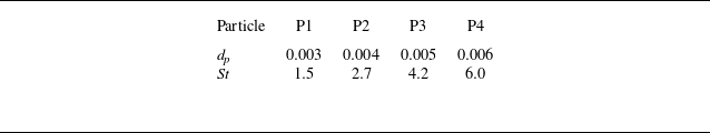


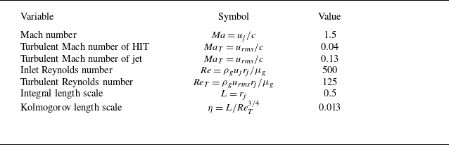
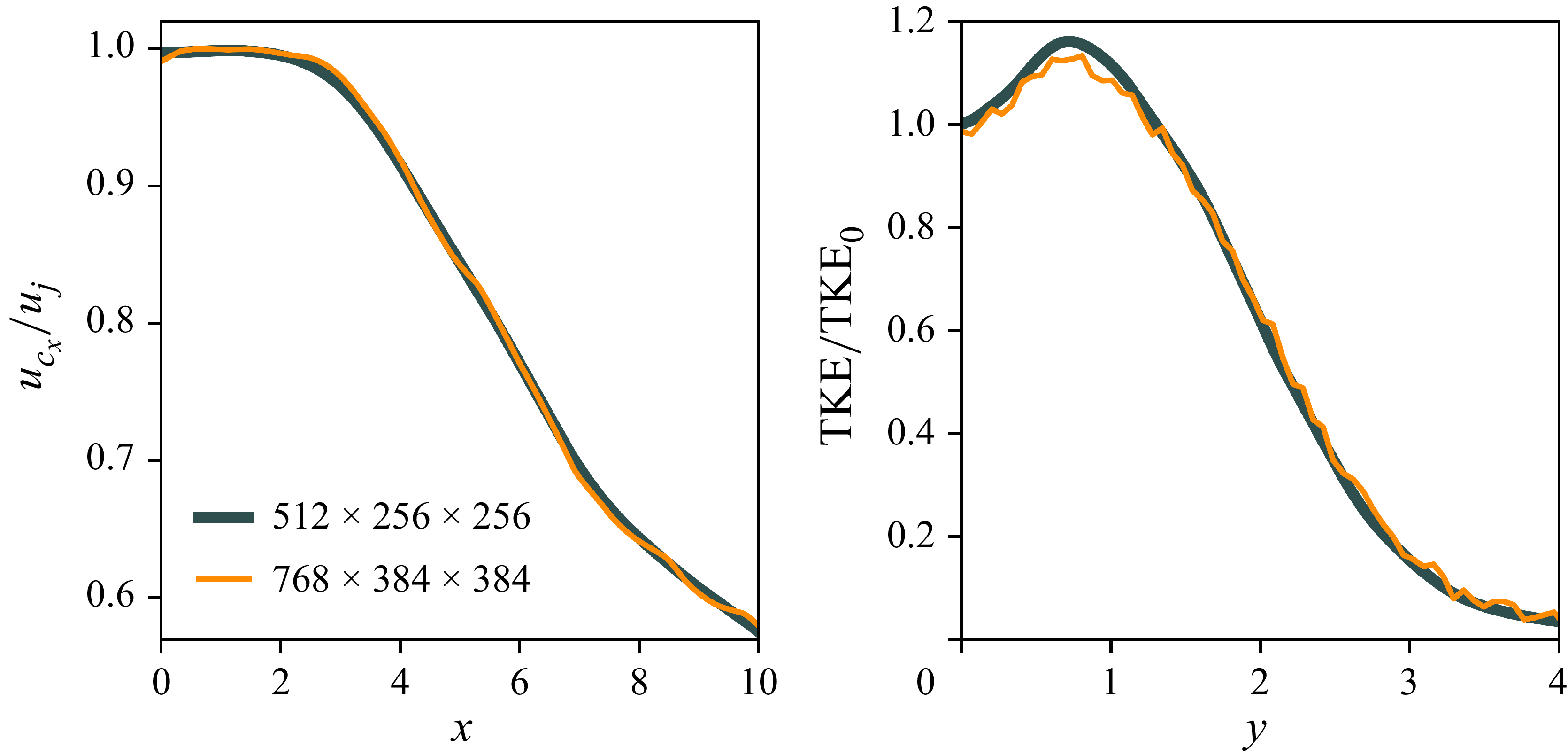


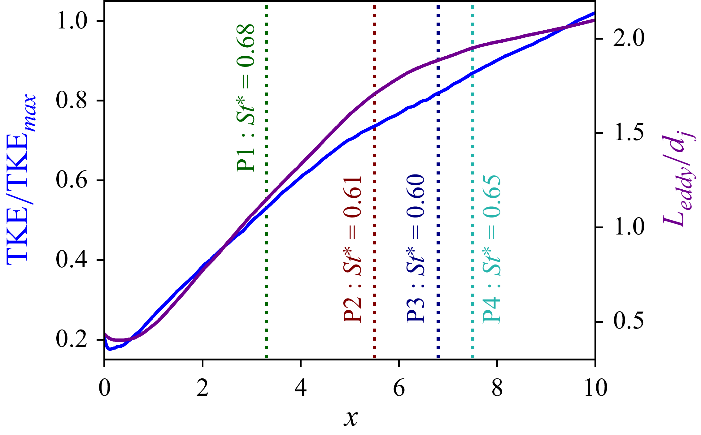


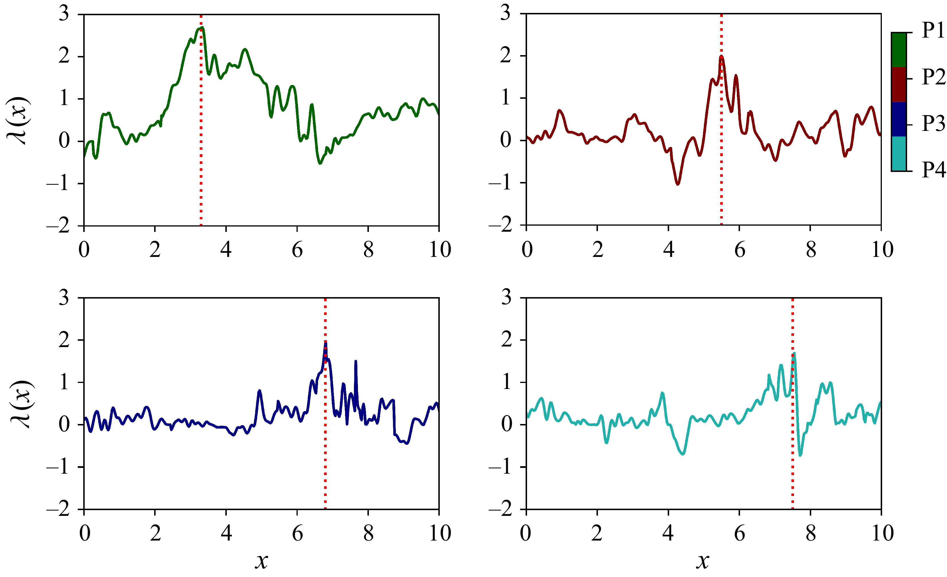


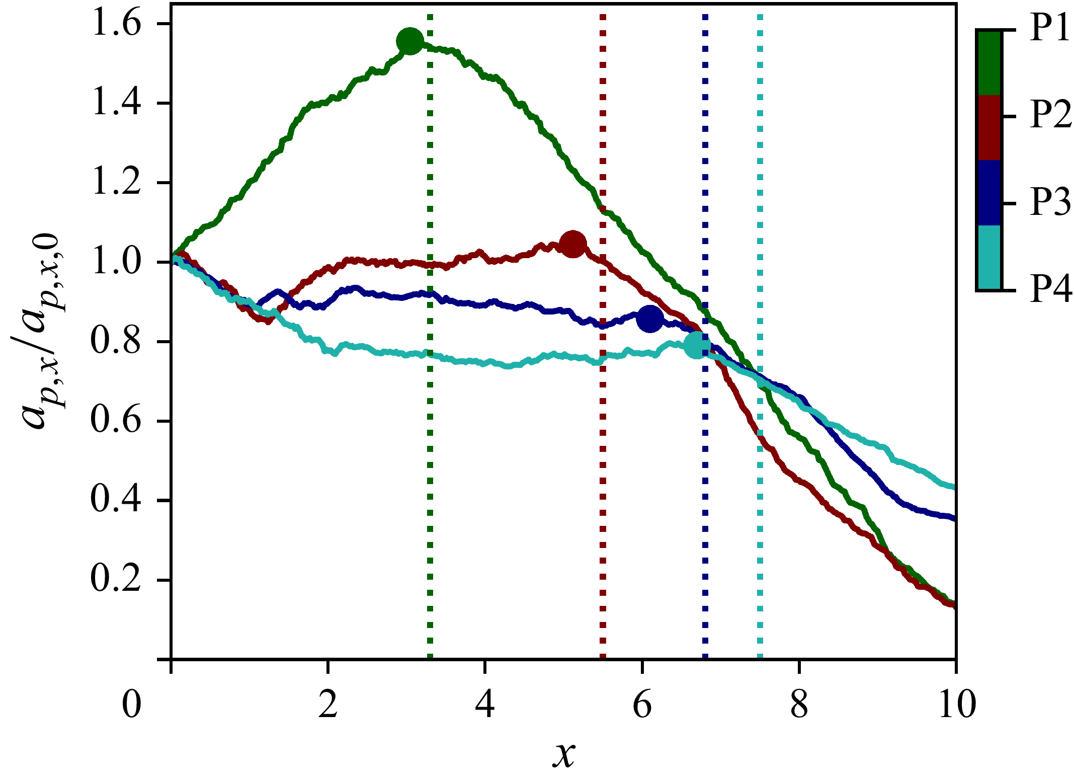


 Open access