


1. Introduction
The structure and the dynamics of turbulent boundary layers (TBLs) under varying pressure gradients (PGs) are influenced by local boundary conditions (BCs) and evolving pressure distributions (Klewicki et al. Reference Klewicki, Sandberg, Knopp, Devenport, Fritsch, Vishwanathan, Volino, Toxopeus, McKeon and Eca2024). The review by Devenport & Lowe (Reference Devenport and Lowe2022), on the impact of local BCs and upstream histories on TBLs development, demonstrated that each location within the TBL is influenced by cumulative upstream effects, as real-world boundary layers rarely encounter uniform PGs. A constant $\beta$
, the Clauser PG parameter (Clauser Reference Clauser1954) (where
$\beta$
, the Clauser PG parameter (Clauser Reference Clauser1954) (where $\beta = [\delta ^*/\tau _w][{\rm d}p/{\rm d}x]$
with
$\beta = [\delta ^*/\tau _w][{\rm d}p/{\rm d}x]$
with ${\rm d}p/{\rm d}x$
is the streamwise PG,
${\rm d}p/{\rm d}x$
is the streamwise PG, $\delta ^*$
the displacement thickness and
$\delta ^*$
the displacement thickness and $\tau _w$
the wall-shear stress) indicates a near-equilibrium state that is challenging to achieve in turbulent flows due to the presence of inner and outer layers. If considering only the outer region, then, the approximate similarity is reachable for high
$\tau _w$
the wall-shear stress) indicates a near-equilibrium state that is challenging to achieve in turbulent flows due to the presence of inner and outer layers. If considering only the outer region, then, the approximate similarity is reachable for high $\textit{Re}$
. In a non-equilibrium state, TBLs are significantly affected by history of
$\textit{Re}$
. In a non-equilibrium state, TBLs are significantly affected by history of $\beta$
(i.e. variation of
$\beta$
(i.e. variation of $\beta$
with streamwise distance), with the inner and outer layers exhibiting different responses to PG variations. Rapid changes in
$\beta$
with streamwise distance), with the inner and outer layers exhibiting different responses to PG variations. Rapid changes in $\beta$
create history effects in shear stress levels (Spalart & Watmuff Reference Spalart and Watmuff1993; Harun et al. Reference Harun, Monty, Mathis and Marusic2013), even when the mean velocity profiles appear self-similar in the streamwise direction. Additionally, Tsuji & Morikawa (Reference Tsuji and Morikawa1976) demonstrated that fluctuating BCs can result in deviations from the classical log law, further complicating the behaviour of TBLs under non-equilibrium conditions.
$\beta$
create history effects in shear stress levels (Spalart & Watmuff Reference Spalart and Watmuff1993; Harun et al. Reference Harun, Monty, Mathis and Marusic2013), even when the mean velocity profiles appear self-similar in the streamwise direction. Additionally, Tsuji & Morikawa (Reference Tsuji and Morikawa1976) demonstrated that fluctuating BCs can result in deviations from the classical log law, further complicating the behaviour of TBLs under non-equilibrium conditions.
Through large-eddy simulations (LES), Bobke et al. (Reference Bobke, Vinuesa, Örlü and Schlatter2017) expanded on the influence of pressure histories by comparing turbulence statistics for different cases with matched local $\beta$
and
$\beta$
and $\textit{Re}_\tau$
. They observed that at a given streamwise location, non-uniform profiles of
$\textit{Re}_\tau$
. They observed that at a given streamwise location, non-uniform profiles of $\beta =\beta (x)$
result in a weaker wake region and a lower amplitude of the outer peak in the streamwise velocity fluctuations compared with quasiequilibrium flows with constant
$\beta =\beta (x)$
result in a weaker wake region and a lower amplitude of the outer peak in the streamwise velocity fluctuations compared with quasiequilibrium flows with constant $\beta$
. This observation suggests that a single parameter, such as the local value of
$\beta$
. This observation suggests that a single parameter, such as the local value of $\beta$
, is insufficient to fully define the turbulence state in non-equilibrium TBLs (Monty, Harun & Marusic Reference Monty, Harun and Marusic2011; Schlatter & Örlü Reference Schlatter and Örlü2012). Additional parameters are needed to capture the influence of flow history accurately (Perry, Marusic & Jones Reference Perry, Marusic and Jones2002). It should be noted that for a given streamwise location, the viscous sublayer remains relatively unaffected with upstream changes in
$\beta$
, is insufficient to fully define the turbulence state in non-equilibrium TBLs (Monty, Harun & Marusic Reference Monty, Harun and Marusic2011; Schlatter & Örlü Reference Schlatter and Örlü2012). Additional parameters are needed to capture the influence of flow history accurately (Perry, Marusic & Jones Reference Perry, Marusic and Jones2002). It should be noted that for a given streamwise location, the viscous sublayer remains relatively unaffected with upstream changes in $\beta$
, while the outer region is strongly influenced, leading to changes in turbulence statistics throughout the boundary-layer profile. Therefore, the state of the layer at a given location
$\beta$
, while the outer region is strongly influenced, leading to changes in turbulence statistics throughout the boundary-layer profile. Therefore, the state of the layer at a given location $x$
depends not solely on local
$x$
depends not solely on local $\beta$
at
$\beta$
at $x$
, but on the entire profile of
$x$
, but on the entire profile of $\beta (x)$
up to an arbitrary location
$\beta (x)$
up to an arbitrary location $x$
. Bobke et al. (Reference Bobke, Vinuesa, Örlü and Schlatter2017) also found that moderate changes in
$x$
. Bobke et al. (Reference Bobke, Vinuesa, Örlü and Schlatter2017) also found that moderate changes in $\beta$
require an adjustment length of approximately
$\beta$
require an adjustment length of approximately $7 \delta _{99}$
for the TBL to reach a stable state independent of its initial conditions.
$7 \delta _{99}$
for the TBL to reach a stable state independent of its initial conditions.
Along the same lines, Vishwanathan et al. (Reference Vishwanathan, Fritsch, Lowe and Devenport2023) contributed to this understanding through an experimental study of non-equilibrium flows over smooth and rough surfaces. By systematically varying the PG histories along the underside of a NACA 0012 airfoil, they showed that upstream flow histories strongly influence local flow states. Their findings revealed that the mean velocity and turbulence quantities do not collapse according to self-similarity laws in non-equilibrium states as it would be for an ideal sink flow (Townsend Reference Townsend1976). Instead, a lag in the response of integral quantities, such as momentum and displacement thicknesses, evidences the influence of flow history. This lagged response should be incorporated into any approaches to the closure problem for predicting TBL evolutions under non-equilibrium conditions.
1.1. Predictions in non-equilibrium layers
Predictive models are essential for describing the behaviour of TBLs subjected to different PG histories, as they offer a framework to understand and anticipate complex flow dynamics that arise due to the interaction of large- and small-scale structures. In this regard, Perry et al. (Reference Perry, Marusic and Jones2002) addressed the closure problem for two-dimensional (2-D) TBLs over flat surfaces under non-equilibrium conditions with imposed PGs, focusing on the streamwise evolution of the boundary layer. Their approach relied on classical similarity laws, including the logarithmic law of the wall and Coles’ wake function (Coles Reference Coles1956), combined with the momentum integral equation and mean continuity equation (Perry, Marušić & Li Reference Perry, Marušić and Li1994). Using these formulations, the authors empirically derived a universal parameter space defined by four key variables (Jones, Marusic & Perry Reference Jones, Marusic and Perry2001): $\beta$
,
$\beta$
, $S=1/\sqrt {C_f}$
,
$S=1/\sqrt {C_f}$
, $\Pi$
and
$\Pi$
and $\xi =S \delta (d\Pi /{\rm d}x)$
, governed by
$\xi =S \delta (d\Pi /{\rm d}x)$
, governed by $f_1(\beta, S, \Pi, \xi) = 0$
, which captures the layer state in non-equilibrium conditions, with
$f_1(\beta, S, \Pi, \xi) = 0$
, which captures the layer state in non-equilibrium conditions, with $C_f$
being the skin friction coefficient,
$C_f$
being the skin friction coefficient, $\delta$
the boundary-layer thickness and
$\delta$
the boundary-layer thickness and $\Pi$
the wake strength parameter in Cole’s wake function (Coles Reference Coles1956). This parameter space is derived from sparse experimental data and serves as the basis for predicting the streamwise evolution of the layer via a set of coupled non-autonomous first-order ordinary differential equations (ODEs), provided initial conditions and boundary constraints, such as the free stream velocity or wall static pressure. This approach for describing the streamwise evolution can be expressed in terms of the differential equations (Perry et al. Reference Perry, Marusic and Jones2002)
$\Pi$
the wake strength parameter in Cole’s wake function (Coles Reference Coles1956). This parameter space is derived from sparse experimental data and serves as the basis for predicting the streamwise evolution of the layer via a set of coupled non-autonomous first-order ordinary differential equations (ODEs), provided initial conditions and boundary constraints, such as the free stream velocity or wall static pressure. This approach for describing the streamwise evolution can be expressed in terms of the differential equations (Perry et al. Reference Perry, Marusic and Jones2002) ${\rm d}S/{\rm d}\textit{Re}_{\text{x}} = \phi _1(\Pi, S, \textit{Re}_{\text{x}}, \textit{Re}_{\text{L}})$
and
${\rm d}S/{\rm d}\textit{Re}_{\text{x}} = \phi _1(\Pi, S, \textit{Re}_{\text{x}}, \textit{Re}_{\text{L}})$
and ${\rm d}\Pi /{\rm d}x = \phi _2(\Pi, S, \textit{Re}_{\text{x}}, \textit{Re}_{\text{L}})$
, where
${\rm d}\Pi /{\rm d}x = \phi _2(\Pi, S, \textit{Re}_{\text{x}}, \textit{Re}_{\text{L}})$
, where $\textit{Re}_{\text{x}}$
and
$\textit{Re}_{\text{x}}$
and $\textit{Re}_{\text{L}}$
denote local and integral Reynolds numbers, respectively. This methodology aligns well with the attached eddy hypothesis (Townsend Reference Townsend1976; Perry et al. Reference Perry, Li and Marušić1991, Reference Perry, Marušić and Li1994), which posits that the flow at a point is influenced by the remote transport of eddies within the boundary layer, thereby incorporating non-local effects.
$\textit{Re}_{\text{L}}$
denote local and integral Reynolds numbers, respectively. This methodology aligns well with the attached eddy hypothesis (Townsend Reference Townsend1976; Perry et al. Reference Perry, Li and Marušić1991, Reference Perry, Marušić and Li1994), which posits that the flow at a point is influenced by the remote transport of eddies within the boundary layer, thereby incorporating non-local effects.
Using parameters such as $\beta$
,
$\beta$
, $\Pi$
and
$\Pi$
and $\xi$
, their model effectively distinguishes between equilibrium and non-equilibrium states, providing robust predictions across different flow configurations. In quasiequilibrium flows (Perry et al. Reference Perry, Marušić and Li1994), the parameter
$\xi$
, their model effectively distinguishes between equilibrium and non-equilibrium states, providing robust predictions across different flow configurations. In quasiequilibrium flows (Perry et al. Reference Perry, Marušić and Li1994), the parameter $S$
approaches infinity while
$S$
approaches infinity while $\xi = 0$
since
$\xi = 0$
since ${\rm d}\Pi /{\rm d}x = 0$
. Under these conditions, the reduced space
${\rm d}\Pi /{\rm d}x = 0$
. Under these conditions, the reduced space $f_2(\Pi, \beta, S) = 0$
captures the boundary layer state, effectively lowering the dimensionality from four to three parameters compared with non-equilibrium flows. This dimensional reduction simplifies the problem, highlighting how quasiequilibrium states reduce complexity. For the case of a non-equilibrium state, the framework developed in Perry et al. (Reference Perry, Marusic and Jones2002) further provides a mathematical linkage between
$f_2(\Pi, \beta, S) = 0$
captures the boundary layer state, effectively lowering the dimensionality from four to three parameters compared with non-equilibrium flows. This dimensional reduction simplifies the problem, highlighting how quasiequilibrium states reduce complexity. For the case of a non-equilibrium state, the framework developed in Perry et al. (Reference Perry, Marusic and Jones2002) further provides a mathematical linkage between $S$
,
$S$
, $\beta$
and
$\beta$
and $\xi$
for a specific
$\xi$
for a specific $\Pi$
value, under the assumption of a matching shear stress profile in this parameter space. Their model includes a mapping of isosurfaces of
$\Pi$
value, under the assumption of a matching shear stress profile in this parameter space. Their model includes a mapping of isosurfaces of $\xi$
in the
$\xi$
in the $\Pi$
–
$\Pi$
– $\beta$
–
$\beta$
– $S$
space, relying heavily on the wall-wake formulation for velocity profiles. However, an objective of the current study is to eliminate dependency on this formulation to enhance the flexibility and applicability of the model.
$S$
space, relying heavily on the wall-wake formulation for velocity profiles. However, an objective of the current study is to eliminate dependency on this formulation to enhance the flexibility and applicability of the model.
Monty et al. (Reference Monty, Harun and Marusic2011) explored ways to simplify the parameter space governing TBLs subjected to adverse PGs (APGs). Their study focused on disentangling the effects of key parameters, namely $\beta$
, the friction Reynolds number
$\beta$
, the friction Reynolds number $\textit{Re}_{\tau }$
and the acceleration factor
$\textit{Re}_{\tau }$
and the acceleration factor $K$
, each of which influences the structure and behaviour of the boundary layer under APG conditions. A key finding from Monty et al. (Reference Monty, Harun and Marusic2011) is the modification of the wake region in the mean velocity profile as a result of APGs. Specifically, in APG flows, the wake begins much closer to the wall, and for both mild and strong APGs, there is no well-defined logarithmic region in the velocity profile, as seen in Spalart & Watmuff (Reference Spalart and Watmuff1993) and Nagano, Tsuji & Houra (Reference Nagano, Tsuji and Houra1998). This absence of a log-law region under strong APG conditions challenges the classical understanding based on the log-law formulation, which serves as the foundation of Perry et al. (Reference Perry, Marusic and Jones2002) model. Furthermore, they found that the von Kármán constant
$K$
, each of which influences the structure and behaviour of the boundary layer under APG conditions. A key finding from Monty et al. (Reference Monty, Harun and Marusic2011) is the modification of the wake region in the mean velocity profile as a result of APGs. Specifically, in APG flows, the wake begins much closer to the wall, and for both mild and strong APGs, there is no well-defined logarithmic region in the velocity profile, as seen in Spalart & Watmuff (Reference Spalart and Watmuff1993) and Nagano, Tsuji & Houra (Reference Nagano, Tsuji and Houra1998). This absence of a log-law region under strong APG conditions challenges the classical understanding based on the log-law formulation, which serves as the foundation of Perry et al. (Reference Perry, Marusic and Jones2002) model. Furthermore, they found that the von Kármán constant $\kappa$
, a fundamental constant in the log law, is not universal; instead, it decreases as PGs increase (Nagib & Chauhan Reference Nagib and Chauhan2008). The authors also highlighted several other effects of APGs on TBLs. First, APG flows experience an increase in the wake parameter
$\kappa$
, a fundamental constant in the log law, is not universal; instead, it decreases as PGs increase (Nagib & Chauhan Reference Nagib and Chauhan2008). The authors also highlighted several other effects of APGs on TBLs. First, APG flows experience an increase in the wake parameter $\Pi$
, signifying an intensification of the outer layer wake. Second, the large-scale structures within the TBL become energized under APG conditions, leading to higher turbulence intensity (as seen in Lee Reference Lee2017). Last, they observed strong amplitude modulation, where the large-scale motions substantially influence the small-scale structures within the boundary layer (Marusic, Mathis & Hutchins Reference Marusic, Mathis and Hutchins2010). This modulation further was investigated by Mathis, Hutchins & Marusic (Reference Mathis, Hutchins and Marusic2011) who developed a model to predict turbulence in the inner layer based on measurements of large-scale signatures from the outer region. The authors investigated the influence of PGs on the large-scale structures in the outer region of TBLs and their modulation of the near-wall region. Their findings support the hypothesis that large-scale structures have a significant impact on the entire boundary layer, extending down to the wall in line with Townsend’s attached eddy hypothesis (Reference Townsend1976) . The authors highlight the energetic role of superstructures in the outer region, observed as an outer peak in the premultiplied energy spectra within the logarithmic layer. The magnitude of this peak depends on the Reynolds number, signifying the influence of large scales on near-wall dynamics (Lee Reference Lee2017; Volino Reference Volino2020). This interaction is not a simple superposition of large-scale structures onto small-scale near-wall fluctuations; rather, it involves a modulation of the small-scale turbulence by the large-scale structures present in the logarithmic region. However, they noted that while the model captures overall trends, in strong APG flows its accuracy is reduced. By tuning some model parameters, predictions were improved, but a recalibration is essential for specific flow states.
$\Pi$
, signifying an intensification of the outer layer wake. Second, the large-scale structures within the TBL become energized under APG conditions, leading to higher turbulence intensity (as seen in Lee Reference Lee2017). Last, they observed strong amplitude modulation, where the large-scale motions substantially influence the small-scale structures within the boundary layer (Marusic, Mathis & Hutchins Reference Marusic, Mathis and Hutchins2010). This modulation further was investigated by Mathis, Hutchins & Marusic (Reference Mathis, Hutchins and Marusic2011) who developed a model to predict turbulence in the inner layer based on measurements of large-scale signatures from the outer region. The authors investigated the influence of PGs on the large-scale structures in the outer region of TBLs and their modulation of the near-wall region. Their findings support the hypothesis that large-scale structures have a significant impact on the entire boundary layer, extending down to the wall in line with Townsend’s attached eddy hypothesis (Reference Townsend1976) . The authors highlight the energetic role of superstructures in the outer region, observed as an outer peak in the premultiplied energy spectra within the logarithmic layer. The magnitude of this peak depends on the Reynolds number, signifying the influence of large scales on near-wall dynamics (Lee Reference Lee2017; Volino Reference Volino2020). This interaction is not a simple superposition of large-scale structures onto small-scale near-wall fluctuations; rather, it involves a modulation of the small-scale turbulence by the large-scale structures present in the logarithmic region. However, they noted that while the model captures overall trends, in strong APG flows its accuracy is reduced. By tuning some model parameters, predictions were improved, but a recalibration is essential for specific flow states.
1.2. Possibility of reduced-order spaces
Along the same line, in recent work, Agrawal et al. (Reference Agrawal, Bose, Griffin and Moin2024) advanced this framework by simplifying the multidimensional formulation presented by Perry et al. (Reference Perry, Marusic and Jones2002) into a single first-order ODE, effectively reducing the dimensional complexity of the problem. Agrawal et al. (Reference Agrawal, Bose, Griffin and Moin2024) were inspired by Thwaites’ method (Reference Thwaites1949) for evaluating the evolution of laminar boundary layers under PGs, where the von Kármán momentum integral equation depends mainly on a local flow parameter $m = m(\theta, {\rm d}p/{\rm d}x, U_{\infty })$ $=- ({\theta ^2}/{\mu U_{\infty }})({{\rm d}p}/{{\rm d}x})$
, referred to as the Holstein–Bholen PG parameter (
$=- ({\theta ^2}/{\mu U_{\infty }})({{\rm d}p}/{{\rm d}x})$
, referred to as the Holstein–Bholen PG parameter ( $\mu$
is the dynamic viscosity of the flow). The authors adapted this method for 2-D TBLs, obtaining accurate estimates of the momentum thickness
$\mu$
is the dynamic viscosity of the flow). The authors adapted this method for 2-D TBLs, obtaining accurate estimates of the momentum thickness $\theta$
from the free stream velocity profile. However, the modified Thwaites’ method does not provide information on the evolution of other boundary layer properties, such as the skin friction coefficient, displacement thickness and Clauser’s PG parameter, which defines the strength of the PG relative to the wall shear stress (Clauser Reference Clauser1954). Their closure problem is solved through a least-squares optimization to determine three model coefficients, achieving a best fit with databases that include wall-resolved LES of TBLs subjected to zero (Eitel-Amor, Örlü & Schlatter Reference Eitel-Amor, Örlü and Schlatter2014) and adverse with initial varying PGs (Bobke et al. Reference Bobke, Vinuesa, Örlü and Schlatter2017). This allowed them to predict flow separation points based on PG histories within the boundary layer.
$\theta$
from the free stream velocity profile. However, the modified Thwaites’ method does not provide information on the evolution of other boundary layer properties, such as the skin friction coefficient, displacement thickness and Clauser’s PG parameter, which defines the strength of the PG relative to the wall shear stress (Clauser Reference Clauser1954). Their closure problem is solved through a least-squares optimization to determine three model coefficients, achieving a best fit with databases that include wall-resolved LES of TBLs subjected to zero (Eitel-Amor, Örlü & Schlatter Reference Eitel-Amor, Örlü and Schlatter2014) and adverse with initial varying PGs (Bobke et al. Reference Bobke, Vinuesa, Örlü and Schlatter2017). This allowed them to predict flow separation points based on PG histories within the boundary layer.
Together, the frameworks developed by Perry et al. (Reference Perry, Marusic and Jones2002) and Agrawal et al. (Reference Agrawal, Bose, Griffin and Moin2024) represent substantial advances in modelling TBL evolution under PGs. The present study builds on these contributions by proposing a data-driven model that can enable accurate predictions while bypassing the need for wall-wake formulations. A series of measurements were carried out in high Reynolds numbers that allowed us to make some specific observations on the intergral quantities of the flow. Then, a refined version of the above-mentioned models is proposed to enhance the understanding of TBL dynamics and improve predictive capabilities for engineering systems. The proposed model will allow us to determine streamwise histories of different quantities given external BCs and therefore will provide rapid predictive capabilities that is required for both the set-up of more advanced experiments and numerical simulations. This tool can also be used to potentially predict the skin-friction evolution and thereby the overall drag incurred by PG boundary layers.
The paper is organized in four sections. Section 2 provides descriptions of the experimental measurements. In § 3, we introduce the data-driven modelling paradigm to predict the streamwise evolution of integral quantities of the TBL. The model is calibrated against the measurements outlined in § 2. Validations of the model and extrapolated results on the history effects are presented in §§ 4 and 5.
2. Experiments
The experiments were performed in the Boundary Layer Wind Tunnel at the University of Southampton. This ’Göttingen’-type closed-loop facility features a 12-m-long test section with an internal cross-section of $1.2 \, \text{m} \times 1 \, \text{m}$
, divided into five segments, each 2.4 m in length. A cooling unit ensures the test section is maintained at a constant temperature of 20
$1.2 \, \text{m} \times 1 \, \text{m}$
, divided into five segments, each 2.4 m in length. A cooling unit ensures the test section is maintained at a constant temperature of 20 $^\circ$
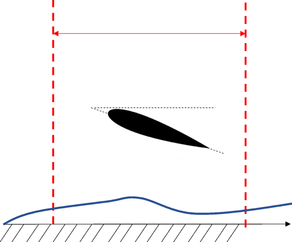
C, providing a stable experimental environment. The free stream turbulence intensity is kept below 0.1 %. Optical access for particle image velocimetry (PIV) is enabled by glass windows enclosing part of the test section. To promote a laminar-to-turbulent transition, a zigzag strip is installed at the test section inlet. To generate PGs on the TBL, a NACA0012 airfoil with a chord length of 1.25 m was installed in the wind tunnel. The leading edge (LE) of the airfoil was positioned 6.53 m downstream of the test section inlet, with a clearance of 500 mm from the wall. This clearance was measured from a quarter of the chord length behind the LE. The angle of attack was remotely adjusted using four linear actuators, mounted in pairs on either side of the airfoil. A Pitot tube is positioned one chord length upstream of the aerofoil’s LE when set to
$^\circ$
C, providing a stable experimental environment. The free stream turbulence intensity is kept below 0.1 %. Optical access for particle image velocimetry (PIV) is enabled by glass windows enclosing part of the test section. To promote a laminar-to-turbulent transition, a zigzag strip is installed at the test section inlet. To generate PGs on the TBL, a NACA0012 airfoil with a chord length of 1.25 m was installed in the wind tunnel. The leading edge (LE) of the airfoil was positioned 6.53 m downstream of the test section inlet, with a clearance of 500 mm from the wall. This clearance was measured from a quarter of the chord length behind the LE. The angle of attack was remotely adjusted using four linear actuators, mounted in pairs on either side of the airfoil. A Pitot tube is positioned one chord length upstream of the aerofoil’s LE when set to $0^\circ$
. The pressure difference is recorded using a Furness FCO560 micromanometer, which establishes
$0^\circ$
. The pressure difference is recorded using a Furness FCO560 micromanometer, which establishes $U_{\infty,0}$
for the experiment. Temperature and pressure at the tunnel inlet are monitored using an RTD TST414 thermometer and a Setra 278 barometric pressure transducer, respectively. For the measurement section, the fourth section of the tunnel is replaced with 10-mm-thick safety glass. This modification serves to provide optical access for wall shear stress measurements. The free stream velocity was set to
$U_{\infty,0}$
for the experiment. Temperature and pressure at the tunnel inlet are monitored using an RTD TST414 thermometer and a Setra 278 barometric pressure transducer, respectively. For the measurement section, the fourth section of the tunnel is replaced with 10-mm-thick safety glass. This modification serves to provide optical access for wall shear stress measurements. The free stream velocity was set to $20 \, \text{ms}^{-1}$
, and the wing was adjusted to five different AOAs: –8
$20 \, \text{ms}^{-1}$
, and the wing was adjusted to five different AOAs: –8 $^\circ$
, –4
$^\circ$
, –4 $^\circ$
, 0
$^\circ$
, 0 $^\circ$
, 4
$^\circ$
, 4 $^\circ$
and 8
$^\circ$
and 8 $^\circ$
.
$^\circ$
.
2.1. Wall pressure measurements
Twenty pressure taps with an inner diameter of 0.6 mm were spaced 0.24 m apart along the floor of the wind tunnel. Panel method calculations indicated that the upstream and downstream influence of the airfoil extended over one chord length. Consequently, the taps were placed to cover the entire region. The mean pressure distribution was recorded using a 64-channel ZOC33/64 Px pressure scanner, with pressure differences referenced to atmospheric pressure. Pressure data was sampled with a frequency of 64 Hz for a scan duration of 90 s. The pneumatic inputs were scanned with a high-speed multiplexer of 50 kHz. The pressure scanner calibration was made in factory, with a relative uncertainty of ${\pm}0.2\,\%$
of full scale (i.e.
${\pm}0.2\,\%$
of full scale (i.e. $\pm 5\,\rm Pa$
). The mean PG distribution for the five angles of attack is presented in figure 1(a). Two distinct history types can be observed. The first type consists of cases with a favourable PG (FPG) followed by an APG (
$\pm 5\,\rm Pa$
). The mean PG distribution for the five angles of attack is presented in figure 1(a). Two distinct history types can be observed. The first type consists of cases with a favourable PG (FPG) followed by an APG ( $-8^\circ$
,
$-8^\circ$
, $-4^\circ$
,
$-4^\circ$
, $0^\circ$
). The second type includes cases with an APG followed by an FPG (
$0^\circ$
). The second type includes cases with an APG followed by an FPG ( $4^\circ$
,
$4^\circ$
, $8^\circ$
). These cases represent non-equilibrium pressure distributions, as
$8^\circ$
). These cases represent non-equilibrium pressure distributions, as $\beta$
is not constant. The PG histories corroborate the panel method prediction that the influence of the airfoil extends one chord upstream and downstream of the aerofoil.
$\beta$
is not constant. The PG histories corroborate the panel method prediction that the influence of the airfoil extends one chord upstream and downstream of the aerofoil.
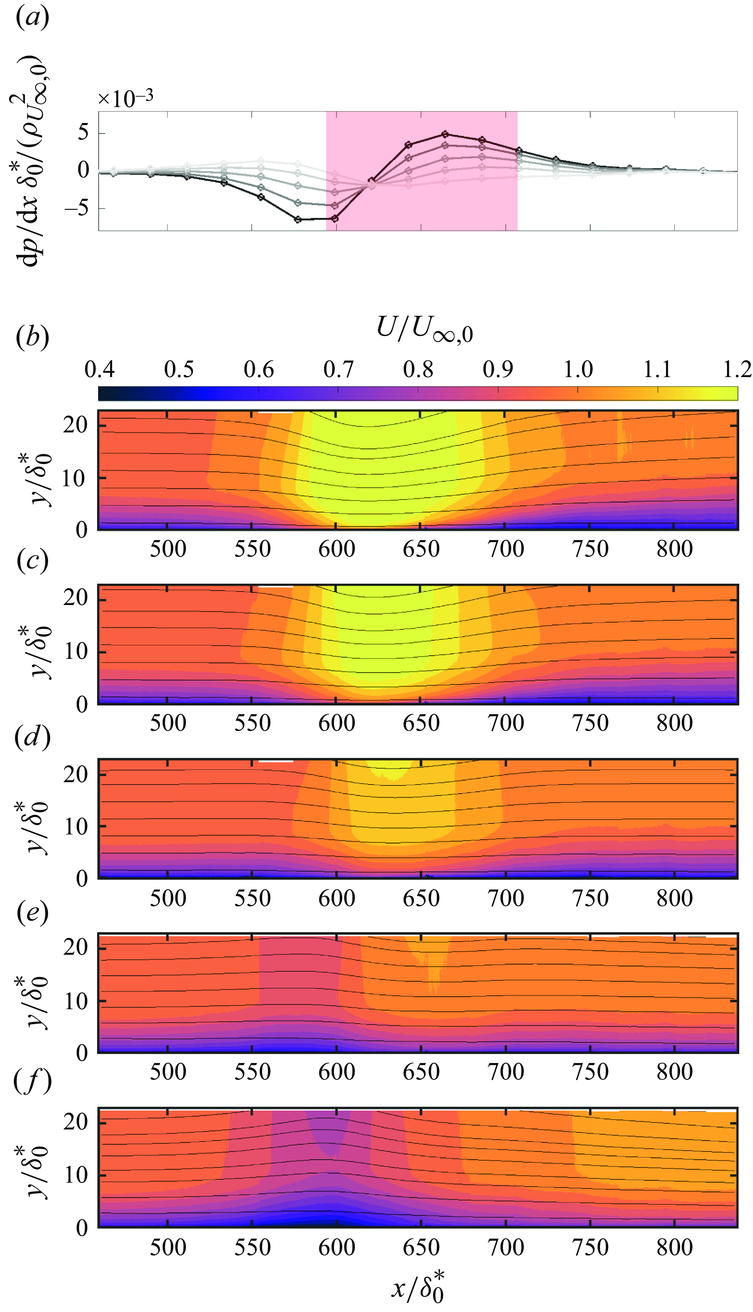
Figure 1. Dimensionless PGs and streamwise velocity fields: (a) PGs at different AOAs (gradients of grey from light to dark, AOA = $8^{\circ }$
,
$8^{\circ }$
, $4^{\circ }$
,
$4^{\circ }$
, $0^{\circ }$
,
$0^{\circ }$
, $-4^{\circ }$
,
$-4^{\circ }$
, $-8^{\circ }$
); (b–f) velocity fields; (b) AOA =
$-8^{\circ }$
); (b–f) velocity fields; (b) AOA = $-8^{\circ }$
; (c) AOA =
$-8^{\circ }$
; (c) AOA = $-4^{\circ }$
; (d) AOA =
$-4^{\circ }$
; (d) AOA = $0^{\circ }$
; (e) AOA =
$0^{\circ }$
; (e) AOA = $4^{\circ }$
; (f) AOA =
$4^{\circ }$
; (f) AOA = $8^{\circ }$
; solid lines, streamlines;
$8^{\circ }$
; solid lines, streamlines; $\delta ^*_0$
is the displacement thickness measured at
$\delta ^*_0$
is the displacement thickness measured at $x_0=4.8m$
; light-red box in (a), region below the airfoil at AOA = 0
$x_0=4.8m$
; light-red box in (a), region below the airfoil at AOA = 0 $^\circ$
.
$^\circ$
.
2.2. Particle image velocimetry
High-resolution planar PIV measurements were conducted to capture the flow fields for the specified cases. The imaging set-up included four 25 MP cameras (LaVision Imager sCMOS) equipped with 50 mm lenses. A Litron Bernoulli PIV series laser (LPU550) and JEM Pro-Fog were used as the light source and seeding particles, respectively. The laser beam was directed through a hole in the wind tunnel floor and guided to the region of interest using mirrors. To shape the laser sheet along the streamwise direction, two spherical lenses ( $f = -75\,\text{mm}$
and
$f = -75\,\text{mm}$
and $f = 150\,\text{mm}$
) and a cylindrical lens (
$f = 150\,\text{mm}$
) and a cylindrical lens ( $f = -20\,\text{mm}$
) were positioned inside the tunnel far downstream of the trailing edge of the wing. This configuration not only corrected laser beam divergence but also ensured a consistent beam thickness of approximately
$f = -20\,\text{mm}$
) were positioned inside the tunnel far downstream of the trailing edge of the wing. This configuration not only corrected laser beam divergence but also ensured a consistent beam thickness of approximately $1.5\,\text{mm}$
throughout the investigation region. The system was triggered internally using a LaVision programmable timing unit (PTU-X). For each airfoil AOA, the procedure was made four times by shifting the position of the cameras streamwise to cover the full region of interest.
$1.5\,\text{mm}$
throughout the investigation region. The system was triggered internally using a LaVision programmable timing unit (PTU-X). For each airfoil AOA, the procedure was made four times by shifting the position of the cameras streamwise to cover the full region of interest.
For each case, 2000 images were sampled at a rate of 0.5 Hz. The low acquisition frequency was chosen to ensure minimally time-correlated samples and to utilize the highest beam quality achievable by the laser. The PIV set-up was configured for a maximum particle displacement of 15 pixels in the free stream and 5–6 pixels in the near-wall region. The particle diameters ranged from 1 to 3 pixels, with lenses f-stop adjusted in the range $f/\# = 1.8$
to
$f/\# = 1.8$
to $f/\# = 4.0$
. This adjustment maximized the cross-correlation coefficient while minimizing peak locking. The depth of field was approximately
$f/\# = 4.0$
. This adjustment maximized the cross-correlation coefficient while minimizing peak locking. The depth of field was approximately $2.5\,\text{mm}$
. Data acquisition was through DaVis 10 software, whereas the preprocessing and postprocessing was made with an in-house code to perform filtering of the images (min subtraction and min/max normalization), cross-correlation of the double frame images, median test and stitching of the four PIV fields. Image cross-correlation employed interrogation windows of
$2.5\,\text{mm}$
. Data acquisition was through DaVis 10 software, whereas the preprocessing and postprocessing was made with an in-house code to perform filtering of the images (min subtraction and min/max normalization), cross-correlation of the double frame images, median test and stitching of the four PIV fields. Image cross-correlation employed interrogation windows of $64 \times 64$
pixels for the first pass and
$64 \times 64$
pixels for the first pass and $16 \times 16$
pixels for the final pass, with
$16 \times 16$
pixels for the final pass, with $50\, \%$
overlap. The resulting field of view covered an area of approximately
$50\, \%$
overlap. The resulting field of view covered an area of approximately $4.5\,\rm m \times 0.3\,\rm m$
. The spatial resolution achieved was
$4.5\,\rm m \times 0.3\,\rm m$
. The spatial resolution achieved was $1\,\text{mm}$
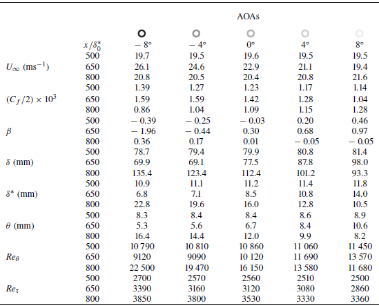
per final interrogation window. A summary of the experimental results is shown in table 1.
$1\,\text{mm}$
per final interrogation window. A summary of the experimental results is shown in table 1.
Table 1. Summary of the measurements taken at $x/\delta ^*_0=500, 650, 800$
for the five different AOAs. Each AOA is labelled with circles with different shades of grey;
$x/\delta ^*_0=500, 650, 800$
for the five different AOAs. Each AOA is labelled with circles with different shades of grey; $\delta ^*_0$
is the displacement thickness measured at
$\delta ^*_0$
is the displacement thickness measured at $x_0=4.8m$
,
$x_0=4.8m$
, $\textit{Re}_{\tau }=u_{\tau }\delta /\nu$
and
$\textit{Re}_{\tau }=u_{\tau }\delta /\nu$
and $\textit{Re}_{\theta }=U_{\infty } \theta /\nu$
.
$\textit{Re}_{\theta }=U_{\infty } \theta /\nu$
.
The final measured mean streamwise velocity fields are shown in figure 1(b–f) for the five different AOAs. The evolution of the boundary layer is evidently strongly influenced by the history of the imposed PG. For the FPG–APG cases, the boundary layer is seen to get thinner and then thicker and vice versa for APG–FPG cases (see the streamlines in figure 1). It appears as though the boundary layer is shaped or modulated by the external PG. This fact is used later in § 3. The strongest alteration of the streamlines occurs at the extreme angles of attack, specifically at $\text{AOA} = -8^\circ$
and
$\text{AOA} = -8^\circ$
and $\text{AOA} = +8^\circ$
, and this has implications for how PG histories shape the development of the boundary layer. Downstream the trailing edge, positioned at
$\text{AOA} = +8^\circ$
, and this has implications for how PG histories shape the development of the boundary layer. Downstream the trailing edge, positioned at $ x/\delta ^*_{0} = 710$
, upstream variations in PG histories continue to influence changes in streamline density beyond
$ x/\delta ^*_{0} = 710$
, upstream variations in PG histories continue to influence changes in streamline density beyond $ x/\delta ^*_{0} = 800$
(see figure 1
b–f), despite comparable local PGs in this region (figure 1
a). This observation is supported by the displacement thickness evolution beneath the airfoil, as presented in figure 2, where the TBL downstream the airfoil TE responds distinctly to different upstream PG profiles, thereby altering the integral parameter
$ x/\delta ^*_{0} = 800$
(see figure 1
b–f), despite comparable local PGs in this region (figure 1
a). This observation is supported by the displacement thickness evolution beneath the airfoil, as presented in figure 2, where the TBL downstream the airfoil TE responds distinctly to different upstream PG profiles, thereby altering the integral parameter $\delta ^*$
. As these modifications flow effectively ‘remembers’ its prior conditions, resulting in delayed responses that persist well beyond the well beyond the immediate vicinity of the wing. This lag is further illustrated in figure 3, where the measured displacement thickness values are compared with a zero-pressure-gradient (ZPG) reference. Under mild PGs at
$\delta ^*$
. As these modifications flow effectively ‘remembers’ its prior conditions, resulting in delayed responses that persist well beyond the well beyond the immediate vicinity of the wing. This lag is further illustrated in figure 3, where the measured displacement thickness values are compared with a zero-pressure-gradient (ZPG) reference. Under mild PGs at $\text{AOA} = 0^\circ$
, the flow deviates from the ZPG case mainly beneath the wing, then rapidly returns to near-ZPG conditions downstream of the trailing edge. In contrast, stronger PGs at
$\text{AOA} = 0^\circ$
, the flow deviates from the ZPG case mainly beneath the wing, then rapidly returns to near-ZPG conditions downstream of the trailing edge. In contrast, stronger PGs at $\text{AOA} = \pm 8^\circ$
induce more substantial and enduring differences, as the TBL adjusts not merely to the local conditions but to the entire history of imposed PGs. Therefore, the TBL changes that lead to significant departures from a ZPG state in integral parameters, such as
$\text{AOA} = \pm 8^\circ$
induce more substantial and enduring differences, as the TBL adjusts not merely to the local conditions but to the entire history of imposed PGs. Therefore, the TBL changes that lead to significant departures from a ZPG state in integral parameters, such as $\delta ^*$
and
$\delta ^*$
and $\theta$
, persisting far downstream of the original disturbances.
$\theta$
, persisting far downstream of the original disturbances.
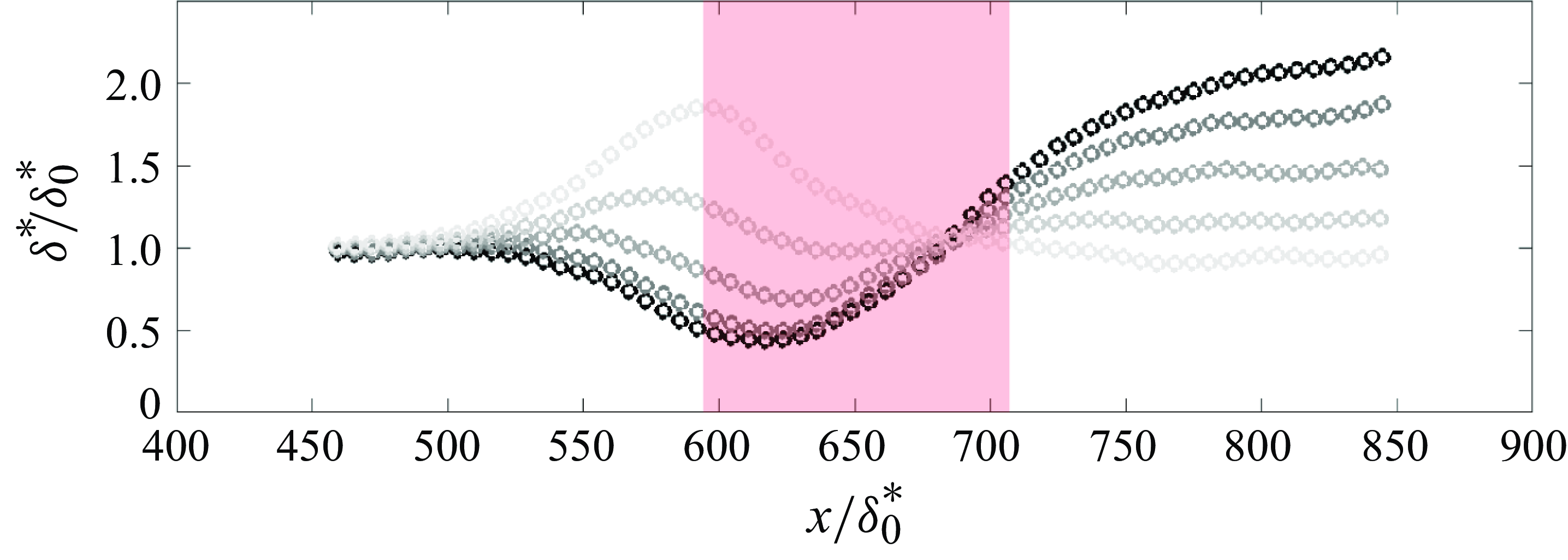
Figure 2. Dimensionless displacement thickness distributions: gradients of grey from light to dark, AOA = $8^{\circ }$
,
$8^{\circ }$
, $4^{\circ }$
,
$4^{\circ }$
, $0^{\circ }$
,
$0^{\circ }$
, $-4^{\circ }$
,
$-4^{\circ }$
, $-8^{\circ }$
;
$-8^{\circ }$
; $\delta ^*_0$
is the displacement thickness measured at
$\delta ^*_0$
is the displacement thickness measured at $x_0=4.8m$
; light-red box, region below the airfoil at AOA = 0
$x_0=4.8m$
; light-red box, region below the airfoil at AOA = 0 $^\circ$
.
$^\circ$
.
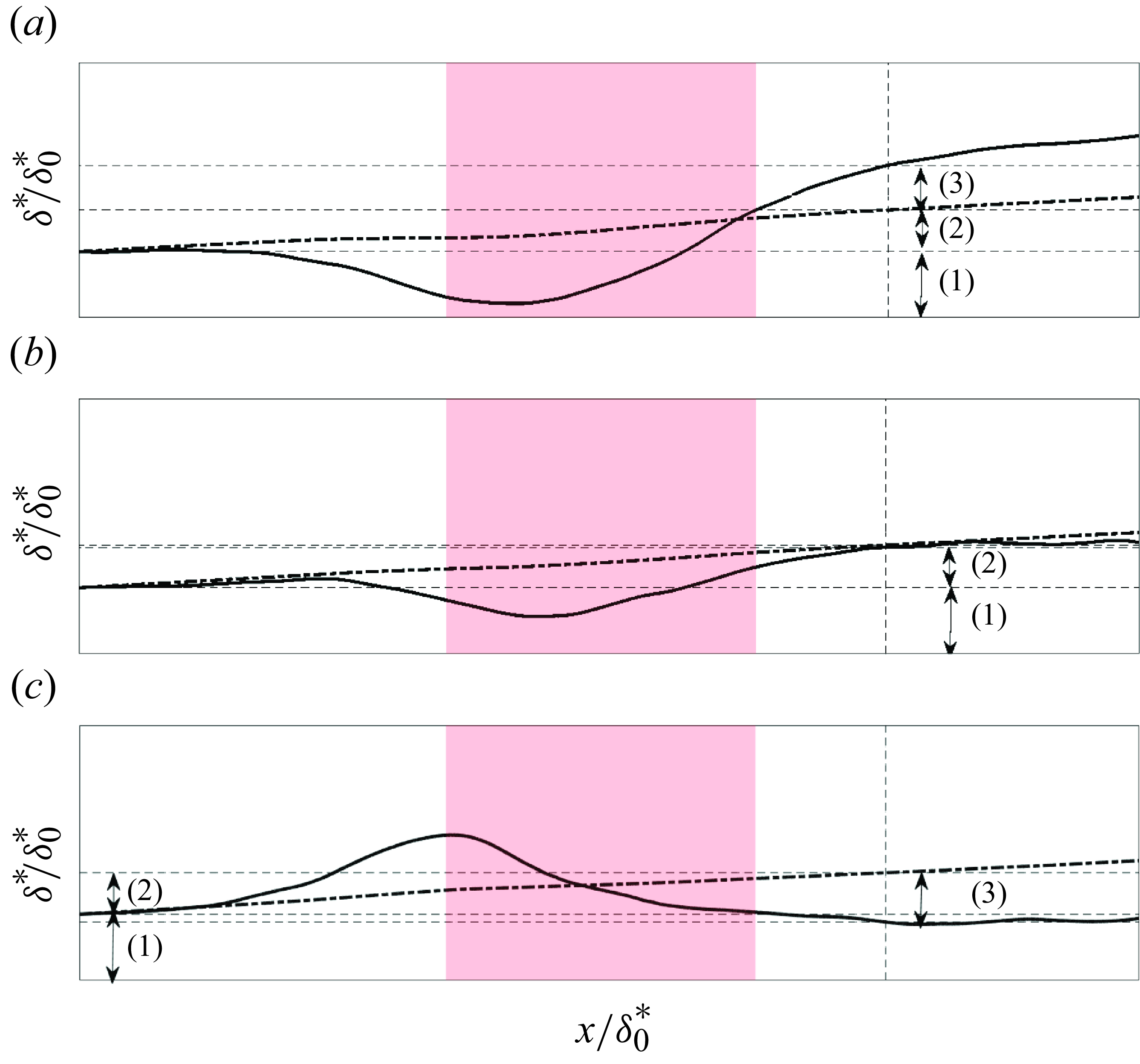
Figure 3. Schematics for the comparison between the displacement thicknesses generated under the wing (solid line) and the ones computed with the equation (Vinuesa et al. Reference Vinuesa, Örlü, Sanmiguel Vila, Ianiro, Discetti and Schlatter2017) for a ZPG case (dash–dotted line): (a) AOA = $-8{^\circ }$
; (b) AOA =
$-8{^\circ }$
; (b) AOA = $0{^\circ }$
; (c) AOA =
$0{^\circ }$
; (c) AOA = $8{^\circ }$
; (1)
$8{^\circ }$
; (1) $\delta ^*/\delta ^*_0=1$
; (2)
$\delta ^*/\delta ^*_0=1$
; (2) $\displaystyle ({\Delta \delta ^*_{ZPG}(x/\delta ^*_0)})/{\delta ^*_0}$
; (3)
$\displaystyle ({\Delta \delta ^*_{ZPG}(x/\delta ^*_0)})/{\delta ^*_0}$
; (3) $\displaystyle \int _{x_0/\delta ^*_0}^{x/\delta ^*_0} (A(x/\delta ^*_0)\cdot {(\delta ^*(x/\delta ^*_0))}/({\delta ^*_0})d(x/\delta ^*_0))$
.
$\displaystyle \int _{x_0/\delta ^*_0}^{x/\delta ^*_0} (A(x/\delta ^*_0)\cdot {(\delta ^*(x/\delta ^*_0))}/({\delta ^*_0})d(x/\delta ^*_0))$
.
2.3. Oil film interferometry
In addition to velocity fields, oil film interferometry (OFI) is applied to directly measure skin friction (Lozier et al. Reference Lozier, Zarei, Deshpande and Marusic2024). Unlike methods that rely on the universality of the logarithmic law, OFI evaluates wall shear stress without such assumptions. The wall shear stress, $\tau _w$
, is determined from the thinning rate of an oil film applied to the surface. The temporal variation of the oil thickness is inferred from changes in the spacing of interference fringes, produced by illuminating the oil layer with monochromatic light and capturing the fringe pattern with an angled camera. This, in turn, can be converted to shear-stress information (Chauhan, Ng & Marusic Reference Chauhan, Ng and Marusic2010; Segalini, Rüedi & Monkewitz Reference Segalini, Rüedi and Monkewitz2015).
$\tau _w$
, is determined from the thinning rate of an oil film applied to the surface. The temporal variation of the oil thickness is inferred from changes in the spacing of interference fringes, produced by illuminating the oil layer with monochromatic light and capturing the fringe pattern with an angled camera. This, in turn, can be converted to shear-stress information (Chauhan, Ng & Marusic Reference Chauhan, Ng and Marusic2010; Segalini, Rüedi & Monkewitz Reference Segalini, Rüedi and Monkewitz2015).
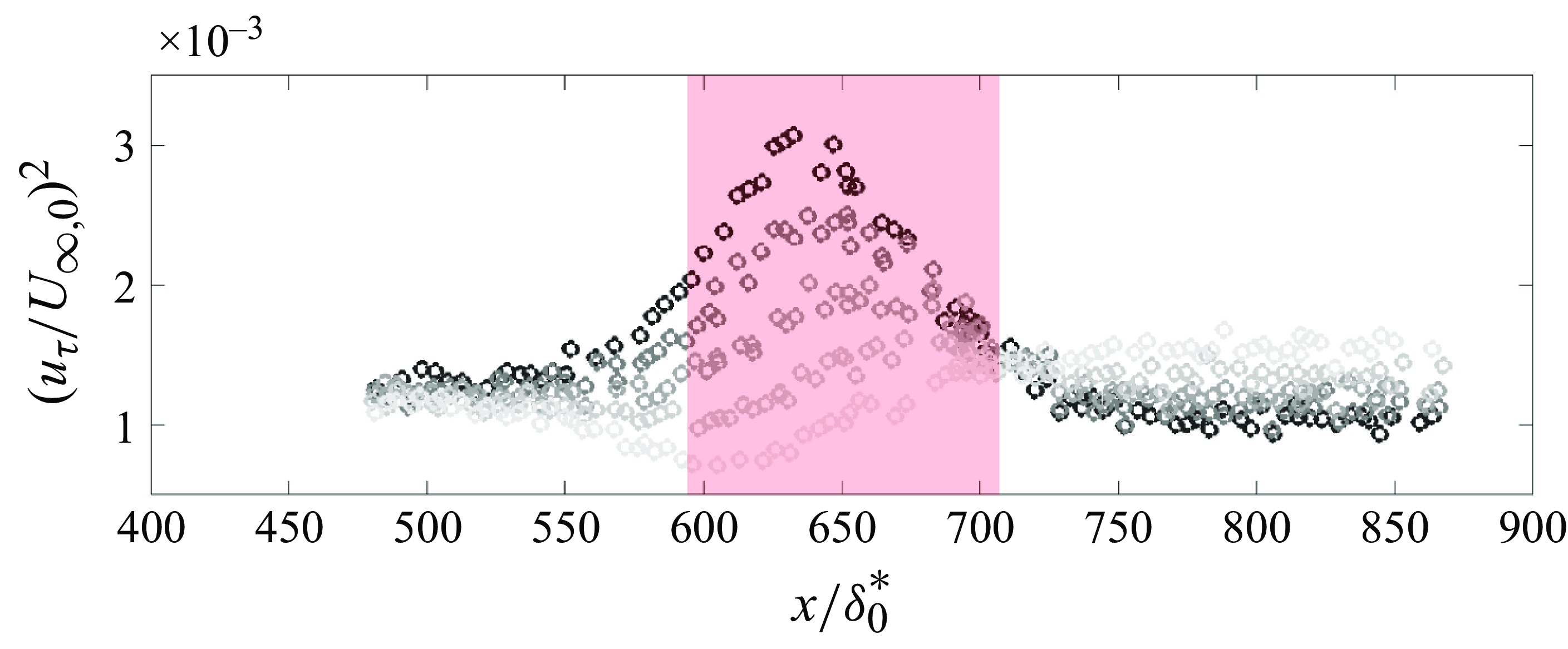
Figure 4. Wall shear stress measurements: gradients of grey from light to dark, AOA = $8^{\circ }$
,
$8^{\circ }$
, $4^{\circ }$
,
$4^{\circ }$
, $0^{\circ }$
,
$0^{\circ }$
, $-4^{\circ }$
,
$-4^{\circ }$
, $-8^{\circ }$
; light-red box, region below the airfoil at AOA = 0
$-8^{\circ }$
; light-red box, region below the airfoil at AOA = 0 $^\circ$
;
$^\circ$
; $U_{\infty,0}$
, free stream velocity at
$U_{\infty,0}$
, free stream velocity at $x_0$
;
$x_0$
; $u_{\tau }$
, friction velocity.
$u_{\tau }$
, friction velocity.

Figure 5. Measured Clauser parameter of the TBLs developing underneath the wing: (a) $\beta$
versus
$\beta$
versus $x/\delta ^*_0$
; (b)
$x/\delta ^*_0$
; (b) $\beta$
versus
$\beta$
versus $\textit{Re}_{\theta }=\theta U_{\infty }/\nu$
; light-red box, region below the airfoil at AOA = 0
$\textit{Re}_{\theta }=\theta U_{\infty }/\nu$
; light-red box, region below the airfoil at AOA = 0 $^\circ$
; gradients of grey from light to dark, AOA =
$^\circ$
; gradients of grey from light to dark, AOA = $8^{\circ }$
,
$8^{\circ }$
, $4^{\circ }$
,
$4^{\circ }$
, $0^{\circ }$
,
$0^{\circ }$
, $-4^{\circ }$
,
$-4^{\circ }$
, $-8^{\circ }$
.
$-8^{\circ }$
.
Silicon-based oil (Polycraft Dow Corning 200/50 Silicone Fluid) was used to generate the interference fringes, which were imaged using two LaVision Imager ProLX 16 MP cameras equipped with Sigma 105 mm F2.8 lenses. A Phillips 35W SOX-E bulb provided the monochromatic light source. The spatial frequency of the fringe patterns was extracted by applying a continuous wavelet transform to the intensity profile $I(x)$
of the captured images, recorded at 1 Hz (Aguiar Ferreira et al. Reference Aguiar Ferreira, Costa and Ganapathisubramani2024). A Morse wavelet (Lilly Reference Lilly2017) with a symmetry parameter of 3, a time-bandwidth product of 60 and a frequency scale resolution of 48 voices-per-octave was used for the analysis. Each measurement spanned a region of approximately 30 cm and was repeated 16 times to cover a streamwise length of nearly 4.5 m, for every AOA of the wing. The results are shown in figure 4 in terms of dimensionless friction velocity
$I(x)$
of the captured images, recorded at 1 Hz (Aguiar Ferreira et al. Reference Aguiar Ferreira, Costa and Ganapathisubramani2024). A Morse wavelet (Lilly Reference Lilly2017) with a symmetry parameter of 3, a time-bandwidth product of 60 and a frequency scale resolution of 48 voices-per-octave was used for the analysis. Each measurement spanned a region of approximately 30 cm and was repeated 16 times to cover a streamwise length of nearly 4.5 m, for every AOA of the wing. The results are shown in figure 4 in terms of dimensionless friction velocity $u_{\tau }$
. The relative uncertainty of the OFI measurements was estimated to be
$u_{\tau }$
. The relative uncertainty of the OFI measurements was estimated to be $\pm 3\, \%$
(Pailhas et al. Reference Pailhas, Barricau, Touvet and Perret2009).
$\pm 3\, \%$
(Pailhas et al. Reference Pailhas, Barricau, Touvet and Perret2009).
At $AOA=-8^{\circ }$
, the initial FPG accelerates the TBL, causing an increase in friction velocity
$AOA=-8^{\circ }$
, the initial FPG accelerates the TBL, causing an increase in friction velocity $u_{\tau }$
up to a maximum at
$u_{\tau }$
up to a maximum at $x/\delta _{0}^{*} = 625$
. Subsequently, due to the generated APG, the flow decelerates and the friction velocity decreases, approaching uniform values for
$x/\delta _{0}^{*} = 625$
. Subsequently, due to the generated APG, the flow decelerates and the friction velocity decreases, approaching uniform values for $x/\delta _{0}^{*} \gt 750$
. As the
$x/\delta _{0}^{*} \gt 750$
. As the $AOA$
increases, this initial rise in
$AOA$
increases, this initial rise in $u_{\tau }$
diminishes. At both
$u_{\tau }$
diminishes. At both $AOA=4^{\circ }$
and
$AOA=4^{\circ }$
and $AOA=8^{\circ }$
, the trend is reversed: the initial APG lowers
$AOA=8^{\circ }$
, the trend is reversed: the initial APG lowers $u_{\tau }$
, which then subsequently increases as the flow accelerates, reaching uniform values from
$u_{\tau }$
, which then subsequently increases as the flow accelerates, reaching uniform values from $x/\delta _{0}^{*} \gt 725$
, ultimately exceeding those observed for
$x/\delta _{0}^{*} \gt 725$
, ultimately exceeding those observed for $AOA=-8^{\circ }$
. The modulation of
$AOA=-8^{\circ }$
. The modulation of $u_{\tau }$
due to negative
$u_{\tau }$
due to negative $AOA$
values is greater than that for positive
$AOA$
values is greater than that for positive $AOA=4^{\circ }$
and
$AOA=4^{\circ }$
and $AOA=8^{\circ }$
.
$AOA=8^{\circ }$
.
By combining spatially resolved $u_{\tau }$
measurements with
$u_{\tau }$
measurements with $\delta ^{*}$
from PIV, it is possible to reconstruct the complete Clauser parameter (
$\delta ^{*}$
from PIV, it is possible to reconstruct the complete Clauser parameter ( $\beta$
) history of the TBL beneath the wing for all five
$\beta$
) history of the TBL beneath the wing for all five $AOA$
values (see figure 5
a). This
$AOA$
values (see figure 5
a). This $\beta$
history spans a region of approximately 4.5 m and is obtained entirely from measurements, without invoking log-fitting methods to extrapolate
$\beta$
history spans a region of approximately 4.5 m and is obtained entirely from measurements, without invoking log-fitting methods to extrapolate $u_{\tau }$
from velocity profiles. Due to the complexity of the OFI over long streamwise distances, obtaining extensive
$u_{\tau }$
from velocity profiles. Due to the complexity of the OFI over long streamwise distances, obtaining extensive $\beta$
histories over large streamwise fetches requires significant effort. Typically, authors derive
$\beta$
histories over large streamwise fetches requires significant effort. Typically, authors derive $u_{\tau }$
from log-fitting velocity profiles (Vishwanathan et al. Reference Vishwanathan, Fritsch, Lowe and Devenport2023). Comparing the
$u_{\tau }$
from log-fitting velocity profiles (Vishwanathan et al. Reference Vishwanathan, Fritsch, Lowe and Devenport2023). Comparing the $\beta$
profiles with the
$\beta$
profiles with the ${\rm d}p/{\rm d}x$
distributions (see figure 1
a) reveals that the intersection of trends for different
${\rm d}p/{\rm d}x$
distributions (see figure 1
a) reveals that the intersection of trends for different $AOA$
values occurs immediately at the LE for
$AOA$
values occurs immediately at the LE for $\beta$
, while the dimensionless
$\beta$
, while the dimensionless ${\rm d}p/{\rm d}x$
curves intersect slightly downstream. Similar to
${\rm d}p/{\rm d}x$
curves intersect slightly downstream. Similar to ${\rm d}p/{\rm d}x$
, downstream of the TE,
${\rm d}p/{\rm d}x$
, downstream of the TE, $\beta$
gradually returns to zero for
$\beta$
gradually returns to zero for $x/\delta _{0}^{*} \gt 820$
. Additional observations (see figure 5
a) indicate that it is not sufficient to define the TBL state based solely on local
$x/\delta _{0}^{*} \gt 820$
. Additional observations (see figure 5
a) indicate that it is not sufficient to define the TBL state based solely on local $\beta$
: at
$\beta$
: at $x/\delta _{0}^{*}=600$
, different
$x/\delta _{0}^{*}=600$
, different $AOA$
values yield the same local
$AOA$
values yield the same local $\beta$
, yet
$\beta$
, yet $\delta ^{*}$
and
$\delta ^{*}$
and $u_{\tau }$
differ, showing that
$u_{\tau }$
differ, showing that $\beta$
alone does not fully characterize the TBL state. Even incorporating the local gradient
$\beta$
alone does not fully characterize the TBL state. Even incorporating the local gradient $d\beta /{\rm d}x$
is not enough, since beyond
$d\beta /{\rm d}x$
is not enough, since beyond $x/\delta _{0}^{*} \gt 825$
, the TBLs share similar
$x/\delta _{0}^{*} \gt 825$
, the TBLs share similar $\beta$
values and gradients but differ in integral parameters (see
$\beta$
values and gradients but differ in integral parameters (see $\delta ^{*}$
in figure 2) and
$\delta ^{*}$
in figure 2) and $u_{\tau }$
(see figure 4). Thus, a third parameter is needed to account for the upstream
$u_{\tau }$
(see figure 4). Thus, a third parameter is needed to account for the upstream $\beta$
history. In the next section, we will elaborate on defining a three-parameter space that can uniquely characterize the state of a non-equilibrium TBL.
$\beta$
history. In the next section, we will elaborate on defining a three-parameter space that can uniquely characterize the state of a non-equilibrium TBL.
For quasi-near-equilibrium TBLs, Vinuesa et al. (Reference Vinuesa, Örlü, Sanmiguel Vila, Ianiro, Discetti and Schlatter2017) introduced $\textit{Re}_{\theta }$
, together with
$\textit{Re}_{\theta }$
, together with $\beta$
, as a parameter to describe the state of the developing layer. This will also be the case when the flow typically has one type of PG (FPG or APG) where the boundary layer state changes monotonically (i.e. increasing or decreasing
$\beta$
, as a parameter to describe the state of the developing layer. This will also be the case when the flow typically has one type of PG (FPG or APG) where the boundary layer state changes monotonically (i.e. increasing or decreasing $\theta$
for a given
$\theta$
for a given $U_{\infty }$
). In flows with complex histories such as the one presented here, the relationship between
$U_{\infty }$
). In flows with complex histories such as the one presented here, the relationship between $\beta$
and
$\beta$
and $\textit{Re}_{\theta }$
is non-trivial. Simply knowing
$\textit{Re}_{\theta }$
is non-trivial. Simply knowing $\beta$
and
$\beta$
and $\textit{Re}_{\theta }$
at a given streamwise location does not yield a unique solution for the layer’s state. This complexity is illustrated in figure 5(b), where the trajectories of
$\textit{Re}_{\theta }$
at a given streamwise location does not yield a unique solution for the layer’s state. This complexity is illustrated in figure 5(b), where the trajectories of $\beta$
versus
$\beta$
versus $\textit{Re}_{\theta }$
for different angles of attack intersect or overlap in certain regions of the flow. These observations suggest that each state of the layer follows a specific trajectory, influenced not only by the local flow conditions but also by its upstream history. In other words, accurately predicting future states of the TBL requires incorporating the spatial evolution of
$\textit{Re}_{\theta }$
for different angles of attack intersect or overlap in certain regions of the flow. These observations suggest that each state of the layer follows a specific trajectory, influenced not only by the local flow conditions but also by its upstream history. In other words, accurately predicting future states of the TBL requires incorporating the spatial evolution of $\beta$
, rather than relying solely on local parameter values. This is explored further in the next section.
$\beta$
, rather than relying solely on local parameter values. This is explored further in the next section.
3. Data-driven model for streamwise evolution of integral quantities
The goal is to develop a model to predict streamwise evolution of integral quantities. A data-driven approach should account for the complex history effects. The starting point for such a model is the ‘von Kármán’ momentum integral equation, initially derived by Gruschwitz (Schlichting Reference Schlichting1951) and later by von Kármán (Van Le Reference Van Le1952) that obtained by integrating the Navier–Stokes equations across the boundary-layer thickness. This equation is an under-determined system with one equation and three unknowns: momentum thickness, displacement thickness and skin friction coefficient; while $U_{\infty }(x)$
and
$U_{\infty }(x)$
and ${\rm d}p/{\rm d}x$
are given as BCs,
${\rm d}p/{\rm d}x$
are given as BCs,
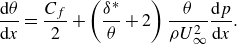 \begin{equation} \frac {{\rm d}\theta }{{\rm d}x} = \frac {C_f}{2} + \left (\frac {\delta ^*}{\theta } + 2\right) \frac {\theta }{\rho U_{\infty }^2}\frac {{\rm d}p}{{\rm d}x}. \end{equation}
To close this system, assumptions on $C_f$
and
$C_f$
and $\delta ^*$
are typically required. Here, we propose data-driven closures for these two quantities. This approach is similar to the recent model proposed by Agrawal et al. (Reference Agrawal, Bose, Griffin and Moin2024), who described the streamwise evolution of the momentum thickness in non-equilibrium TBLs under arbitrary PGs, with
$\delta ^*$
are typically required. Here, we propose data-driven closures for these two quantities. This approach is similar to the recent model proposed by Agrawal et al. (Reference Agrawal, Bose, Griffin and Moin2024), who described the streamwise evolution of the momentum thickness in non-equilibrium TBLs under arbitrary PGs, with ${\rm d}\theta /{\rm d}x = f(m, \textit{Re}_{\theta })$
,
${\rm d}\theta /{\rm d}x = f(m, \textit{Re}_{\theta })$
,
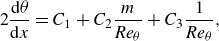 \begin{equation} 2 \frac {{\rm d}\theta }{{\rm d}x} = C_1 + C_2 \frac {m}{\textit{Re}_{\theta }} + C_3\frac {1}{\textit{Re}_{\theta }}, \end{equation}
where $C_1$
,
$C_1$
, $C_2$
and
$C_2$
and $C_3$
are constants fitted to LES results for zero and APG cases (Eitel-Amor et al. Reference Eitel-Amor, Örlü and Schlatter2014; Bobke et al. Reference Bobke, Vinuesa, Örlü and Schlatter2017). Although this model accurately predicts the evolution of momentum thickness within a reasonable uncertainty, it does not fully determine the state of the boundary layer; information about the evolution of skin friction, displacement thickness and
$C_3$
are constants fitted to LES results for zero and APG cases (Eitel-Amor et al. Reference Eitel-Amor, Örlü and Schlatter2014; Bobke et al. Reference Bobke, Vinuesa, Örlü and Schlatter2017). Although this model accurately predicts the evolution of momentum thickness within a reasonable uncertainty, it does not fully determine the state of the boundary layer; information about the evolution of skin friction, displacement thickness and $\beta (x)$
is implicit in the constants
$\beta (x)$
is implicit in the constants $C_1$
,
$C_1$
, $C_2$
and
$C_2$
and $C_3$
. The closure model we propose is based on observations of the data presented in § 2. We hypothesise that the state of a non-equilibrium layer can be represented by the superposition of an equivalent state of a TBL under ZPG conditions, combined with the cumulative ‘lag effects’ produced by the upstream distribution of the PG,
$C_3$
. The closure model we propose is based on observations of the data presented in § 2. We hypothesise that the state of a non-equilibrium layer can be represented by the superposition of an equivalent state of a TBL under ZPG conditions, combined with the cumulative ‘lag effects’ produced by the upstream distribution of the PG, ${\rm d}p/{\rm d}x$
. This linear superposition is illustrated in figure 3(a–c), showing the contributions of the ZPG component (labelled as (2) in the caption of figure 3) and the lag effects (labelled as (3) in the caption of figure 3) to the total displacement thickness as it evolves under different PG distributions.
${\rm d}p/{\rm d}x$
. This linear superposition is illustrated in figure 3(a–c), showing the contributions of the ZPG component (labelled as (2) in the caption of figure 3) and the lag effects (labelled as (3) in the caption of figure 3) to the total displacement thickness as it evolves under different PG distributions.
Consider a TBL developing over a flat plate positioned below an airfoil, which generates varying PG distributions as a function of the AOA of the airfoil. As stated before, figure 3(a–c) illustrate the displacement thickness resulting from the airfoil NACA0012 mounted 500 mm above the wall at AOA values of $-8^\circ$
, 0
$-8^\circ$
, 0 $^\circ$
and 8
$^\circ$
and 8 $^\circ$
, respectively. As outlined in § 2, the displacement thicknesses deviate significantly from the trends expected under ZPG conditions. Following figure 3, at a given dimensionless streamwise location
$^\circ$
, respectively. As outlined in § 2, the displacement thicknesses deviate significantly from the trends expected under ZPG conditions. Following figure 3, at a given dimensionless streamwise location $ x^{\prime} = x/\delta ^*_0$
(where
$ x^{\prime} = x/\delta ^*_0$
(where $ \delta ^*_0$
is the displacement thickness at
$ \delta ^*_0$
is the displacement thickness at $ x = x_0$
), the dimensionless displacement thickness (
$ x = x_0$
), the dimensionless displacement thickness ( $\delta ^*/\delta ^*_0$
) is given by the sum of three components,
$\delta ^*/\delta ^*_0$
) is given by the sum of three components,
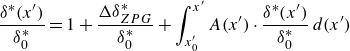 \begin{equation} \frac {\delta ^*( x^{\prime})}{\delta ^*_0} = 1 + \frac {\Delta \delta ^*_{ZPG}}{\delta ^*_0} + \int _{x^{\prime}_0}^{ x^{\prime}} A( x^{\prime}) \cdot \frac {\delta ^*( x^{\prime})}{\delta ^*_0} \, d( x^{\prime}) \end{equation}
where
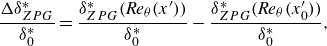 \begin{equation} \frac {\Delta \delta ^*_{ZPG}}{\delta ^*_0} = \frac {\delta ^*_{ZPG}(\textit{Re}_\theta ( x^{\prime}))}{\delta ^*_0} - \frac {\delta ^*_{ZPG}(\textit{Re}_{\theta }(x^{\prime}_0))}{\delta ^*_0}, \end{equation}
where $ A(x^{\prime})$
is a weighting function that evaluates the contribution to
$ A(x^{\prime})$
is a weighting function that evaluates the contribution to $\delta ^*(x^{\prime})/\delta ^*_0$
of each upstream value from
$\delta ^*(x^{\prime})/\delta ^*_0$
of each upstream value from $x^{\prime}_0$
. It is, therefore, a function that accounts for the effects of PG histories as the TBL evolves in the streamwise direction. The functions
$x^{\prime}_0$
. It is, therefore, a function that accounts for the effects of PG histories as the TBL evolves in the streamwise direction. The functions $\delta ^*_{ZPG}(\textit{Re}_{\theta })$
are evaluated according to Vinuesa et al. (Reference Vinuesa, Örlü, Sanmiguel Vila, Ianiro, Discetti and Schlatter2017). Differentiating (3.3) with respect to
$\delta ^*_{ZPG}(\textit{Re}_{\theta })$
are evaluated according to Vinuesa et al. (Reference Vinuesa, Örlü, Sanmiguel Vila, Ianiro, Discetti and Schlatter2017). Differentiating (3.3) with respect to $ x^{\prime}$
, we obtain
$ x^{\prime}$
, we obtain
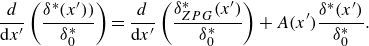 \begin{equation} \frac {d}{{\rm d}x^{\prime}}\left (\frac {\delta ^*( x^{\prime}))}{\delta ^*_0}\right) = \frac {d}{{\rm d}x^{\prime}} \left (\frac {\delta ^*_{ZPG}( x^{\prime})}{\delta ^*_0}\right) + A( x^{\prime}) \frac {\delta ^*( x^{\prime})}{\delta ^*_0}. \end{equation}
Equation (3.5) is a first-order linear non-homogeneous ODE in terms of $ \delta ^*/\delta ^*_0$
. The ODE is linear since
$ \delta ^*/\delta ^*_0$
. The ODE is linear since $ \delta ^*/\delta ^*_0$
and its derivative appear only to the first power and are not multiplied by each other. This type of ODE is associated with lag models, which are commonly used for dynamic systems that exhibit delayed responses to changes in input. The equation resembles the form
$ \delta ^*/\delta ^*_0$
and its derivative appear only to the first power and are not multiplied by each other. This type of ODE is associated with lag models, which are commonly used for dynamic systems that exhibit delayed responses to changes in input. The equation resembles the form $ {{\rm d}Y}/{{\rm d}X} = a+bY$
, where
$ {{\rm d}Y}/{{\rm d}X} = a+bY$
, where $X$
and
$X$
and $Y$
are generic independent and dependent variables, respectively, and
$Y$
are generic independent and dependent variables, respectively, and $a$
and
$a$
and $b$
are arbitrary coefficients. This equation arises in thermal systems, where temperature evolves gradually due to thermal mass inertia (Incropera et al. Reference Incropera1996), as well as in economic models that describe the relationship between investments and interest rates (Goodwin Reference Goodwin1990). In boundary layer theory, White (Reference White1991) describes a similar lag equation used to account for rapid changes in non-equilibrium flows over flat plates, where integral parameters lag behind equilibrium predictions (i.e. the ZPG state in our case) (Ferziger, Lyrio & Bardina Reference Ferziger, Lyrio and Bardina1982). The same model is applied to the skin-friction coefficient, providing
$b$
are arbitrary coefficients. This equation arises in thermal systems, where temperature evolves gradually due to thermal mass inertia (Incropera et al. Reference Incropera1996), as well as in economic models that describe the relationship between investments and interest rates (Goodwin Reference Goodwin1990). In boundary layer theory, White (Reference White1991) describes a similar lag equation used to account for rapid changes in non-equilibrium flows over flat plates, where integral parameters lag behind equilibrium predictions (i.e. the ZPG state in our case) (Ferziger, Lyrio & Bardina Reference Ferziger, Lyrio and Bardina1982). The same model is applied to the skin-friction coefficient, providing
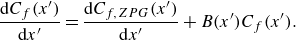 \begin{equation} \frac {{\rm d}C_f( x^{\prime})}{{\rm d}x^{\prime}} = \frac {{\rm d}C_{f,ZPG}( x^{\prime})}{{\rm d}x^{\prime}} + B( x^{\prime}) C_f( x^{\prime}). \end{equation}
The von Kármán momentum integral equation, (3.1), together with (3.5) and (3.6) form a new set of ODEs used to model the streamwise evolution of $\theta /\theta _0$
,
$\theta /\theta _0$
, $ \delta ^*/\delta ^*_0$
and
$ \delta ^*/\delta ^*_0$
and $ C_f$
, providing closure for the problem outlined in the dimensionless form of the momentum integral equation in the streamwise direction
$ C_f$
, providing closure for the problem outlined in the dimensionless form of the momentum integral equation in the streamwise direction $x^{\prime}$
,
$x^{\prime}$
,
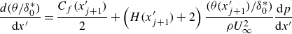 \begin{eqnarray} & \displaystyle \frac {d(\theta /\delta ^*_0)}{{\rm d}x^{\prime}} = \frac {C_f(x^{\prime}_{j+1})}{2} + \left (H(x^{\prime}_{j+1}) + 2\right) \frac {(\theta (x^{\prime}_{j+1})/\delta ^*_0)}{\rho U_{\infty }^2} \frac {{\rm d}p}{{\rm d}x^{\prime}} \end{eqnarray}
where
 \begin{eqnarray} & \displaystyle \frac {\delta ^*(x^{\prime}_{j+1})}{\delta ^*_0} = \displaystyle \frac {\delta ^*(x^{\prime}_{j})}{\delta ^*_0} + \displaystyle \frac {d(\delta ^*/\delta ^*_0)}{d x^{\prime}}(x^{\prime}_{j})\Delta x^{\prime}, \nonumber \\ & \textrm {}\,\,\,C_f(x^{\prime}_{j+1}) = C_f(x^{\prime}_{j}) + \displaystyle \frac {{\rm d}C_f}{{\rm d}x^{\prime}}(x^{\prime}_{j}) \Delta x^{\prime}. \end{eqnarray}
Precisely, the ODEs in (3.5) and (3.6) are used to solve the system in (3.8). The system of equations in (3.7) and (3.8) is solved numerically using an implicit solver with a backward-difference numerical scheme for the derivatives. The integration proceeds in a stepwise manner, starting from the specified initial conditions at $x^{\prime}_0$
. In the above equations, the parameters at
$x^{\prime}_0$
. In the above equations, the parameters at $ (\,j+1)$
are treated as unknowns at the marching step
$ (\,j+1)$
are treated as unknowns at the marching step $ j$
. The system is solved iteratively at each step to determine these unknowns,
$ j$
. The system is solved iteratively at each step to determine these unknowns, $\theta, \delta ^* \text{ and } C_f$
at the step (j
$\theta, \delta ^* \text{ and } C_f$
at the step (j $+$
1) in the one-dimensional (1-D) model. The solution advances downstream with a streamwise step size of
$+$
1) in the one-dimensional (1-D) model. The solution advances downstream with a streamwise step size of $\Delta x^{\prime} = L^{\prime}/1000$
, where
$\Delta x^{\prime} = L^{\prime}/1000$
, where $L^{\prime}= L/\delta ^*_0=400$
is the domain length
$L^{\prime}= L/\delta ^*_0=400$
is the domain length $(L=4.5\,\rm m)$
. To have a unique solution for the system of three equations in (3.7) and (3.8), a set of parameters must be chosen to uniquely define the state of the flow. Following the approach of Perry et al. (Reference Perry, Marusic and Jones2002), we use the dimensionless PG parameter
$(L=4.5\,\rm m)$
. To have a unique solution for the system of three equations in (3.7) and (3.8), a set of parameters must be chosen to uniquely define the state of the flow. Following the approach of Perry et al. (Reference Perry, Marusic and Jones2002), we use the dimensionless PG parameter $ \beta$
to characterize the boundary layer state by incorporating its local value,
$ \beta$
to characterize the boundary layer state by incorporating its local value, $ \beta (x^{\prime}_b)$
, its derivative
$ \beta (x^{\prime}_b)$
, its derivative ${\rm d}\beta /{\rm d}x^{\prime}$
at
${\rm d}\beta /{\rm d}x^{\prime}$
at $ x^{\prime}_b$
, and an integral value,
$ x^{\prime}_b$
, and an integral value, $ \overline {\beta }(x^{\prime}_b)$
, which encapsulates the history of
$ \overline {\beta }(x^{\prime}_b)$
, which encapsulates the history of $ \beta = \beta (x^{\prime})$
up to a streamwise location
$ \beta = \beta (x^{\prime})$
up to a streamwise location $ x^{\prime}_b$
. This last term (
$ x^{\prime}_b$
. This last term ( $ \overline {\beta }(x^{\prime}_b)$
) is computed as a moving average (of
$ \overline {\beta }(x^{\prime}_b)$
) is computed as a moving average (of $\beta$
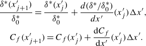
) within a fixed window along the streamwise directions. The mathematical details used to evaluate
$\beta$
) within a fixed window along the streamwise directions. The mathematical details used to evaluate $ \overline {\beta }(x^{\prime}_b)$
are provided in Appendix A.
$ \overline {\beta }(x^{\prime}_b)$
are provided in Appendix A.
Unlike Perry et al. (Reference Perry, Marusic and Jones2002), we propose a new framework that involves a basis change from $ (\beta, S, \Pi, \xi)$
to
$ (\beta, S, \Pi, \xi)$
to $ (\beta, {\rm d}\beta /{\rm d}x^{\prime}, \overline {\beta })$
. Boundary layers that share the same local value of
$ (\beta, {\rm d}\beta /{\rm d}x^{\prime}, \overline {\beta })$
. Boundary layers that share the same local value of $ \beta (x^{\prime}_p)$
and/or the same local gradient but differ in their histories are likely to have distinct structures and states (Lee Reference Lee2017; Bobke et al. Reference Bobke, Vinuesa, Örlü and Schlatter2017). We therefore hypothesize that a developing, non-equilibrium TBL can be fully described by the local value, gradient and integral form of the Clauser dimensionless PG parameter. A single combination of
$ \beta (x^{\prime}_p)$
and/or the same local gradient but differ in their histories are likely to have distinct structures and states (Lee Reference Lee2017; Bobke et al. Reference Bobke, Vinuesa, Örlü and Schlatter2017). We therefore hypothesize that a developing, non-equilibrium TBL can be fully described by the local value, gradient and integral form of the Clauser dimensionless PG parameter. A single combination of $(\beta, {\rm d}\beta /{\rm d}x^{\prime}, \overline {\beta })$
uniquely determines the solution in terms of
$(\beta, {\rm d}\beta /{\rm d}x^{\prime}, \overline {\beta })$
uniquely determines the solution in terms of $\delta ^*, \theta,$
and
$\delta ^*, \theta,$
and $C_f$
. This proportional-differential-integral (PDI) approach characterizes the behaviour of the system, specifically the streamwise evolution of the integral parameters of the TBL as defined in the momentum integral equation, allowing progression in space with the ODE proposed in this work. Note that this model is not intended to predict the velocity statistics, which would require a separate model for the velocity profiles. Therefore, we limit the model to integral quantities.
$C_f$
. This proportional-differential-integral (PDI) approach characterizes the behaviour of the system, specifically the streamwise evolution of the integral parameters of the TBL as defined in the momentum integral equation, allowing progression in space with the ODE proposed in this work. Note that this model is not intended to predict the velocity statistics, which would require a separate model for the velocity profiles. Therefore, we limit the model to integral quantities.
In addition to the PDI system, we also evaluate a reduced-order two-parameter model, which is a proportional-integral approach with a proportional term, $\beta$
, and an integral term,
$\beta$
, and an integral term, $\widetilde {\beta }$
only, used to compensate for slow output responses. This term represents a weighted local average of
$\widetilde {\beta }$
only, used to compensate for slow output responses. This term represents a weighted local average of $ \beta$
, with the weighting function detailed in Appendix A. The three-parameter model, PDI described beforehand, adds a differential term,
$ \beta$
, with the weighting function detailed in Appendix A. The three-parameter model, PDI described beforehand, adds a differential term, ${{\rm d}\beta }/{{\rm d}x}$
, allowing faster reactions to rapid changes. The PDI formulation is fine balance between stability and responsiveness, improving accuracy in systems with both steady and mild
${{\rm d}\beta }/{{\rm d}x}$
, allowing faster reactions to rapid changes. The PDI formulation is fine balance between stability and responsiveness, improving accuracy in systems with both steady and mild $({{\rm d}p}/{{\rm d}x})$
variations. For stable
$({{\rm d}p}/{{\rm d}x})$
variations. For stable $({{\rm d}p}/{{\rm d}x})$
, a proportional-integral controller is preferable. Both the three-parameter and two-parameter spaces, along with the two definitions of the integral form of
$({{\rm d}p}/{{\rm d}x})$
, a proportional-integral controller is preferable. Both the three-parameter and two-parameter spaces, along with the two definitions of the integral form of $\beta$
, namely
$\beta$
, namely $\overline {\beta }$
and
$\overline {\beta }$
and $\widetilde {\beta }$
, are introduced in greater detail in Appendix A. These details are presented in the appendix to prevent the specifics of the model from overshadowing the discussion on the approach.
$\widetilde {\beta }$
, are introduced in greater detail in Appendix A. These details are presented in the appendix to prevent the specifics of the model from overshadowing the discussion on the approach.
4. Calibration and validation of the model
In this section, we first calibrate the model coefficients using the experimental data presented in § 2 for AOAs $-8^\circ$
,
$-8^\circ$
, $0^\circ$
and
$0^\circ$
and $8^\circ$
. Then, the model is applied to predict the non-equilibrium evolution of the TBL for AOAs
$8^\circ$
. Then, the model is applied to predict the non-equilibrium evolution of the TBL for AOAs $-4^\circ$
and
$-4^\circ$
and $4^\circ$
, as well as for quasiequilibrium TBLs from Bobke et al. (Reference Bobke, Vinuesa, Örlü and Schlatter2017), which is necessary for validation.
$4^\circ$
, as well as for quasiequilibrium TBLs from Bobke et al. (Reference Bobke, Vinuesa, Örlü and Schlatter2017), which is necessary for validation.
4.1. Developing TBL underneath a NACA0012: calibration
The calibration of the model involves determining the coefficients $ A(x^{\prime})$
and
$ A(x^{\prime})$
and $ B(x^{\prime})$
in (3.5) and (3.6) as functions of the flow parameters that define the three-dimensional (3-D) space (i.e.
$ B(x^{\prime})$
in (3.5) and (3.6) as functions of the flow parameters that define the three-dimensional (3-D) space (i.e. $ (\beta ( x^{\prime}), \displaystyle ({{\rm d}\beta ( x^{\prime})}/{{\rm d}x^{\prime}}), \overline {\beta }( x^{\prime}))$
defined in Appendix A.1, such that
$ (\beta ( x^{\prime}), \displaystyle ({{\rm d}\beta ( x^{\prime})}/{{\rm d}x^{\prime}}), \overline {\beta }( x^{\prime}))$
defined in Appendix A.1, such that
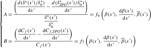 \begin{equation} \begin{cases} A = \frac {\left (\displaystyle \frac {d(\delta ^*( x^{\prime})/\delta ^*_0)}{{\rm d}x^{\prime}} - \frac {d(\delta ^*_{\textit{ZPG}}( x^{\prime})/\delta ^*_0)}{{\rm d}x^{\prime}}\right)}{\displaystyle \frac {\delta ^*( x^{\prime})}{\delta ^*_0}} = f_6\left (\beta ( x^{\prime}), \displaystyle \frac {{\rm d}\beta ( x^{\prime})}{{\rm d}x^{\prime}}, \overline {\beta }( x^{\prime})\right) \\ B = \displaystyle \frac {\left (\displaystyle \frac {{\rm d}C_f( x^{\prime})}{{\rm d}x^{\prime}} - \frac {{\rm d}C_{f,\textit{ZPG}}( x^{\prime})}{{\rm d}x^{\prime}}\right)}{C_f( x^{\prime})} = f_7\left (\beta ( x^{\prime}), \displaystyle \frac {{\rm d}\beta ( x^{\prime})}{{\rm d}x^{\prime}}, \overline {\beta }( x^{\prime})\right) \end{cases} \end{equation}
or in the 2-D space, i.e. $ (\beta ( x^{\prime}), \widetilde {\beta }( x^{\prime}))$
defined in Appendix A.2,
$ (\beta ( x^{\prime}), \widetilde {\beta }( x^{\prime}))$
defined in Appendix A.2,
 \begin{equation} A = f_8\left (\beta ( x^{\prime}), \widetilde {\beta }( x^{\prime})\right) \quad \text{and} \quad B = f_9\left (\beta ( x^{\prime}), \widetilde {\beta }( x^{\prime})\right). \end{equation}
Interpolant functions $ f_6$
and
$ f_6$
and $ f_7$
in the 3-D space (or
$ f_7$
in the 3-D space (or $ f_8$
and
$ f_8$
and $ f_9$
in the reduced-order space) are derived from the sparse experimental datasets in figure 6 using (4.1) and (4.2). The numerators of the two equations in (4.1) are plotted in figures 6(b) and 6(d), where the streamwise derivatives of
$ f_9$
in the reduced-order space) are derived from the sparse experimental datasets in figure 6 using (4.1) and (4.2). The numerators of the two equations in (4.1) are plotted in figures 6(b) and 6(d), where the streamwise derivatives of $ \delta ^*$
and
$ \delta ^*$
and $ C_f$
are compared with their counterparts evaluated under ZPG conditions,
$ C_f$
are compared with their counterparts evaluated under ZPG conditions, $ \delta ^*_{ZPG}$
and
$ \delta ^*_{ZPG}$
and $ C_{f, ZPG}$
. The denominators of the two equations in (4.1) (
$ C_{f, ZPG}$
. The denominators of the two equations in (4.1) ( $ \delta ^*$
and
$ \delta ^*$
and $ C_f$
) are obtained, respectively, from the data shown in figure 6(c) (shape factor
$ C_f$
) are obtained, respectively, from the data shown in figure 6(c) (shape factor $ H$
) and figure 6(a) (dimensionless
$ H$
) and figure 6(a) (dimensionless $ u_{\tau }^2$
). A function is determined to compute the coefficients
$ u_{\tau }^2$
). A function is determined to compute the coefficients $ A$
and
$ A$
and $ B$
in the equations in (4.1) (or 4.2) for each combination of three parameters:
$ B$
in the equations in (4.1) (or 4.2) for each combination of three parameters: $ \beta$
in figure 5(a),
$ \beta$
in figure 5(a), $ {{\rm d}\beta }/{{\rm d}x^{\prime}}$
and either
$ {{\rm d}\beta }/{{\rm d}x^{\prime}}$
and either $ \overline {\beta }$
or
$ \overline {\beta }$
or $ \widetilde {\beta }$
, which are derived and plotted in Appendix A.1 and A.2. A Delaunay triangulation is applied to the scattered data points to enable piecewise linear interpolation and extrapolation within the defined domains.
$ \widetilde {\beta }$
, which are derived and plotted in Appendix A.1 and A.2. A Delaunay triangulation is applied to the scattered data points to enable piecewise linear interpolation and extrapolation within the defined domains.
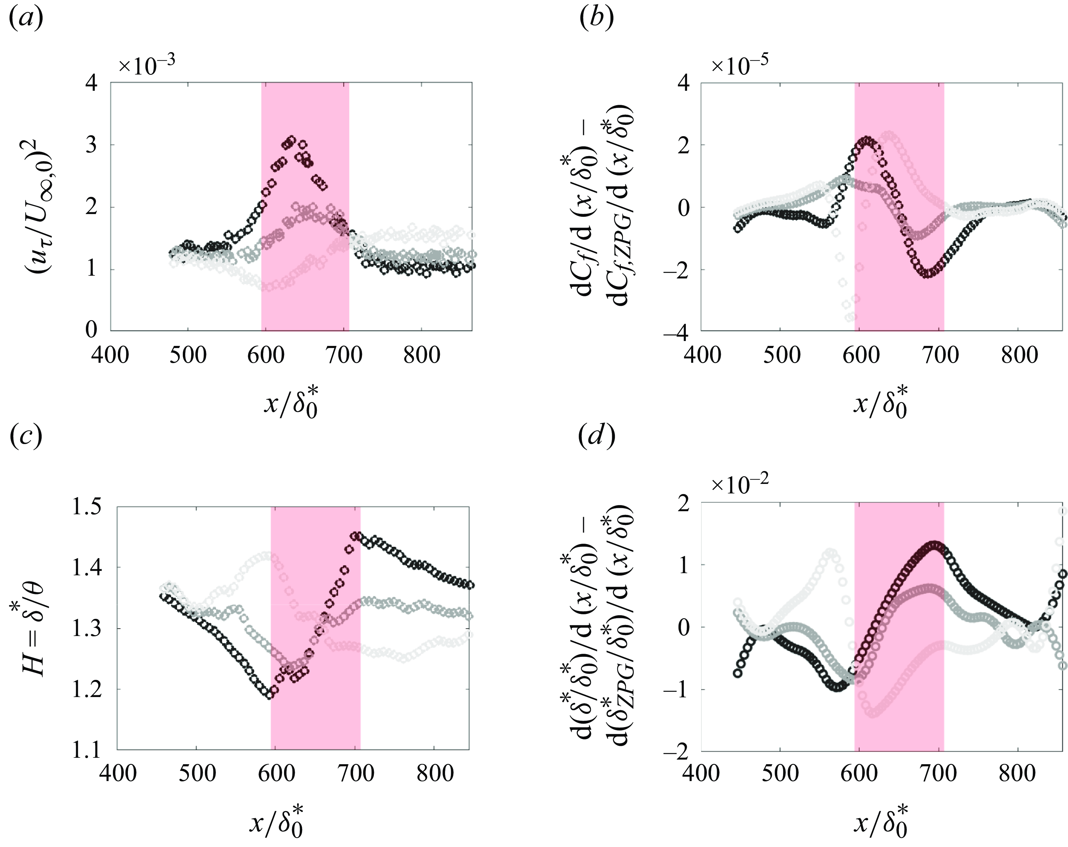
Figure 6. Experimental data used for the calibration of the coefficients A and B of the two ODEs which describe the streamwise evolution of $\delta ^*/\delta ^*_0$
and
$\delta ^*/\delta ^*_0$
and $C_f$
in a TBL developing underneath a NACA0012 wing profile: (a) dimensionless friction velocity; (b) difference between the streamwise derivatives of the skin friction for PG and ZPG TBLs; (c) shape factor
$C_f$
in a TBL developing underneath a NACA0012 wing profile: (a) dimensionless friction velocity; (b) difference between the streamwise derivatives of the skin friction for PG and ZPG TBLs; (c) shape factor $H=\delta ^*/\theta$
; (d) difference between the streamwise derivatives of the displacement thickness for PG and ZPG TBLs; gradients of grey from light to dark, AOA =
$H=\delta ^*/\theta$
; (d) difference between the streamwise derivatives of the displacement thickness for PG and ZPG TBLs; gradients of grey from light to dark, AOA = $8^{\circ }$
,
$8^{\circ }$
, $0^{\circ }$
,
$0^{\circ }$
, $-8^{\circ }$
; light-red box, region below the airfoil at AOA = 0
$-8^{\circ }$
; light-red box, region below the airfoil at AOA = 0 $^\circ$
.
$^\circ$
.
The experimental data used for tuning the model describe the evolution of the non-equilibrium TBL developing over a flat plate, with PG histories generated by a NACA0012 airfoil at AOA of $-8^\circ$
,
$-8^\circ$
, $0^\circ$
and
$0^\circ$
and $8^\circ$
(see figure 6). The streamwise evolution of the derivatives of
$8^\circ$
(see figure 6). The streamwise evolution of the derivatives of $ C_f$
and
$ C_f$
and $ \delta ^*/\delta ^*_0$
reflects the distinct PG distributions induced by the airfoil. These trends are evident in the data, particularly in the departure from ZPG conditions (see figure 6
b,d). The integral parameter
$ \delta ^*/\delta ^*_0$
reflects the distinct PG distributions induced by the airfoil. These trends are evident in the data, particularly in the departure from ZPG conditions (see figure 6
b,d). The integral parameter $\delta ^*_{ZPG}$
and the skin friction coefficient
$\delta ^*_{ZPG}$
and the skin friction coefficient $C_{f, ZPG}$
for the ZPG case are evaluated according to Nagib & Chauhan (Reference Nagib and Chauhan2008) and Vinuesa et al. (Reference Vinuesa, Örlü, Sanmiguel Vila, Ianiro, Discetti and Schlatter2017). The evolution of both the dimensionless displacement thickness
$C_{f, ZPG}$
for the ZPG case are evaluated according to Nagib & Chauhan (Reference Nagib and Chauhan2008) and Vinuesa et al. (Reference Vinuesa, Örlü, Sanmiguel Vila, Ianiro, Discetti and Schlatter2017). The evolution of both the dimensionless displacement thickness $\delta ^*/\theta$
, i.e. shape factor H (see figure 6
c) and of the skin friction (see figure 6
a) reveals significant changes depending on the AOA. For the
$\delta ^*/\theta$
, i.e. shape factor H (see figure 6
c) and of the skin friction (see figure 6
a) reveals significant changes depending on the AOA. For the $-8^\circ$
case, initial acceleration leads to a relative increase in friction velocity compared with the local free stream velocity, resulting in a flatter mean velocity profile and a reduced shape factor. The subsequent deceleration causes a decrease in skin friction and an increase in displacement thickness relative to momentum losses (see figure 6
a,c). The opposite behaviour is observed for
$-8^\circ$
case, initial acceleration leads to a relative increase in friction velocity compared with the local free stream velocity, resulting in a flatter mean velocity profile and a reduced shape factor. The subsequent deceleration causes a decrease in skin friction and an increase in displacement thickness relative to momentum losses (see figure 6
a,c). The opposite behaviour is observed for $ 8^\circ$
, where deceleration precedes acceleration.
$ 8^\circ$
, where deceleration precedes acceleration.
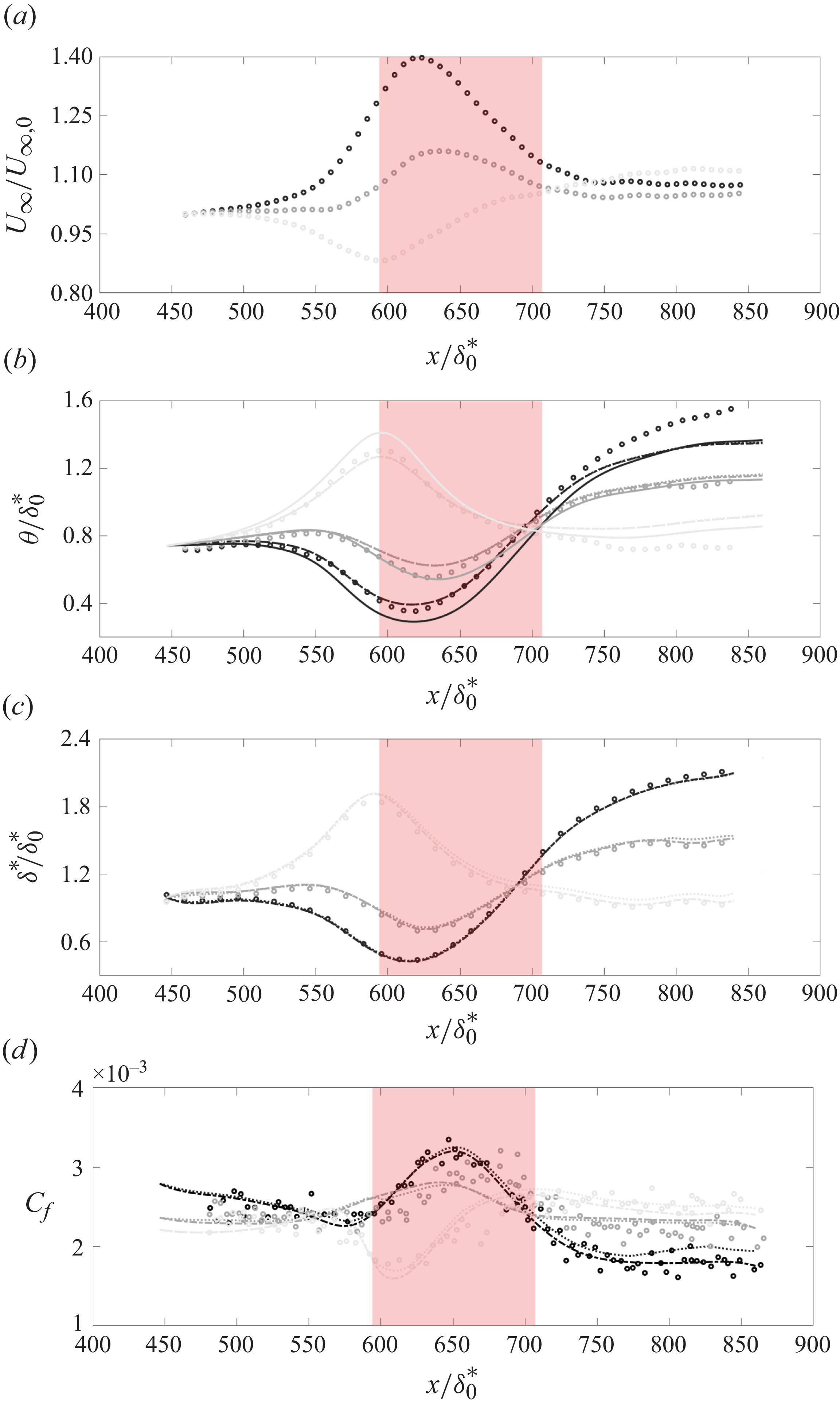
Figure 7. Boundary conditions to the solver and predicted parameters: (a) dimensionless free stream velocity generated underneath the NACA0012 profile; (b) dimensionless momentum thickness; (c) dimensionless displacement thickness; (d) skin friction coefficient; circles, measurements; solid line, prediction by the model in Agrawal et al. (Reference Agrawal, Bose, Griffin and Moin2024); dotted lines, solver defined in the 2-D space; dashed bold lines, solver defined in the 3-D space; gradients of grey from light to dark, AOA = $8^{\circ }$
,
$8^{\circ }$
, $0^{\circ }$
,
$0^{\circ }$
, $-8^{\circ }$
; light-red box, region below the airfoil at AOA = 0
$-8^{\circ }$
; light-red box, region below the airfoil at AOA = 0 $^\circ$
.
$^\circ$
.
The model defined both in the 2-D $(\text{i.e., }\beta ( x^{\prime}), \widetilde {\beta }( x^{\prime}))$
and 3-D (i.e.,
$(\text{i.e., }\beta ( x^{\prime}), \widetilde {\beta }( x^{\prime}))$
and 3-D (i.e., $\beta ( x^{\prime})$
,
$\beta ( x^{\prime})$
, $\displaystyle ({{\rm d}\beta ( x^{\prime})}/{{\rm d}x^{\prime}}), \overline {\beta }( x^{\prime}))$
spaces relies on initial conditions (e.g.
$\displaystyle ({{\rm d}\beta ( x^{\prime})}/{{\rm d}x^{\prime}}), \overline {\beta }( x^{\prime}))$
spaces relies on initial conditions (e.g. $\delta ^*(x^{\prime}_0)/\delta ^*_0$
,
$\delta ^*(x^{\prime}_0)/\delta ^*_0$
, $\theta ^*(x^{\prime}_0)/\delta ^*_0$
,
$\theta ^*(x^{\prime}_0)/\delta ^*_0$
, $C_f(x_0^{\prime})$
,
$C_f(x_0^{\prime})$
, $\beta (x^{\prime}_0)$
) and BCs (e.g.
$\beta (x^{\prime}_0)$
) and BCs (e.g. $ {\rm d}p(x^{\prime})/{\rm d}x^{\prime}$
or
$ {\rm d}p(x^{\prime})/{\rm d}x^{\prime}$
or $ U_\infty (x^{\prime})$
). The streamwise free stream velocity distribution for the three calibration AOAs is shown in figure 7(a), along with the momentum thickness predicted by the modified Thwaites method (Agrawal et al. Reference Agrawal, Bose, Griffin and Moin2024) compared with our experimental PIV data in figure 7(b). While the predictions of the momentum thickness agree well with the overall data, discrepancies are noted near local extrema and downstream of the trailing edge, particularly at
$ U_\infty (x^{\prime})$
). The streamwise free stream velocity distribution for the three calibration AOAs is shown in figure 7(a), along with the momentum thickness predicted by the modified Thwaites method (Agrawal et al. Reference Agrawal, Bose, Griffin and Moin2024) compared with our experimental PIV data in figure 7(b). While the predictions of the momentum thickness agree well with the overall data, discrepancies are noted near local extrema and downstream of the trailing edge, particularly at $-8^\circ$
, where the model underpredicts the TBL recovery, yielding a 15 % error.
$-8^\circ$
, where the model underpredicts the TBL recovery, yielding a 15 % error.
In figures 7(b–d) and 8 the prediction of the model proposed in this work is compared with the experimental data described in § 2. The solver accurately predicts the evolution of the integral parameters ( $\theta$
and
$\theta$
and $\delta ^*$
), the skin friction coefficient (
$\delta ^*$
), the skin friction coefficient ( $C_f$
) and the values of
$C_f$
) and the values of $\beta$
which define the state of the layer and the PG history (
$\beta$
which define the state of the layer and the PG history ( $\beta$
,
$\beta$
, ${{\rm d}\beta }/{{\rm d}x^{\prime}}$
,
${{\rm d}\beta }/{{\rm d}x^{\prime}}$
, $\overline {\beta }$
,
$\overline {\beta }$
, $\widetilde {\beta }$
). Notably, the local maxima and minima of
$\widetilde {\beta }$
). Notably, the local maxima and minima of $\theta$
near the wing are better captured compared with the model by Agrawal et al. (Reference Agrawal, Bose, Griffin and Moin2024). The main difference in predicting
$\theta$
near the wing are better captured compared with the model by Agrawal et al. (Reference Agrawal, Bose, Griffin and Moin2024). The main difference in predicting $\theta$
with Agrawal’s method (Reference Agrawal, Bose, Griffin and Moin2024) is its reduced accuracy at peak values for strong APG and FPG cases at
$\theta$
with Agrawal’s method (Reference Agrawal, Bose, Griffin and Moin2024) is its reduced accuracy at peak values for strong APG and FPG cases at $\text{AOA} = \pm 8^\circ$
. This stems from its calibration with data from Bobke et al. (Reference Bobke, Vinuesa, Örlü and Schlatter2017), where
$\text{AOA} = \pm 8^\circ$
. This stems from its calibration with data from Bobke et al. (Reference Bobke, Vinuesa, Örlü and Schlatter2017), where $\beta$
changes abruptly before stabilizing, unlike our model, which accounts for more gradual variations in
$\beta$
changes abruptly before stabilizing, unlike our model, which accounts for more gradual variations in $({{\rm d}p}/{{\rm d}x})$
. However, for
$({{\rm d}p}/{{\rm d}x})$
. However, for $x^{\prime} \gt 700$
, a slight increase in the predicted momentum thickness error is observed (see figure 7
b). This is attributed to the approximate nature of the von Kármán momentum integral equation, which neglects Reynolds stress derivatives (Wei, Li & Wang Reference Wei, Li and Wang2024).
$x^{\prime} \gt 700$
, a slight increase in the predicted momentum thickness error is observed (see figure 7
b). This is attributed to the approximate nature of the von Kármán momentum integral equation, which neglects Reynolds stress derivatives (Wei, Li & Wang Reference Wei, Li and Wang2024).
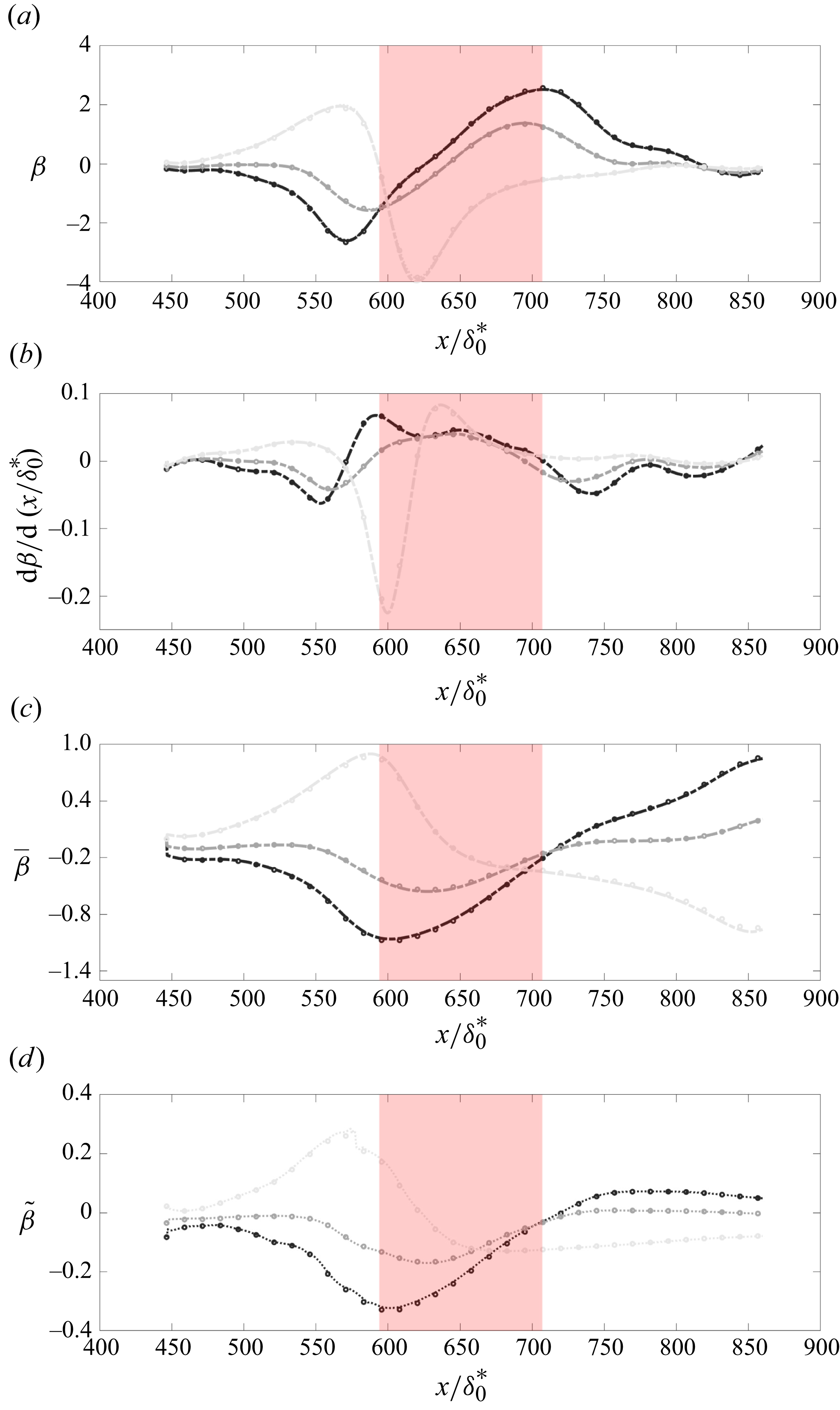
Figure 8. Comparison between calibrated solver and experiments: (a) Clauser parameter $\beta$
; (b) streamwise derivative of
$\beta$
; (b) streamwise derivative of $\beta$
; (c) integral version of
$\beta$
; (c) integral version of $\beta$
according to (A1); (d) integral version of
$\beta$
according to (A1); (d) integral version of $\beta$
according to (A3); circles, experiments; dotted lines, solver defined in the 2-D space; dashed bold lines, solver defined in the 3-D space; gradients of grey from light to dark, AOA =
$\beta$
according to (A3); circles, experiments; dotted lines, solver defined in the 2-D space; dashed bold lines, solver defined in the 3-D space; gradients of grey from light to dark, AOA = $8^{\circ }$
,
$8^{\circ }$
, $0^{\circ }$
,
$0^{\circ }$
, $-8^{\circ }$
; light-red box, region below the airfoil at AOA = 0
$-8^{\circ }$
; light-red box, region below the airfoil at AOA = 0 $^\circ$
.
$^\circ$
.
4.2. Developing TBL underneath a NACA0012: validation
A first attempt to validate the proposed model is conducted by comparing its predictions with the streamwise evolution of the boundary layer underneath the NACA0012 airfoil at angles of attack of $-4^\circ$
and
$-4^\circ$
and $4^\circ$
. It is important to note that the calibration of the model coefficients was performed using data only at AOAs of
$4^\circ$
. It is important to note that the calibration of the model coefficients was performed using data only at AOAs of $-8^\circ$
,
$-8^\circ$
, $0^\circ$
and
$0^\circ$
and $8^\circ$
.
$8^\circ$
.
The input data consists of the free stream velocity distributions generated by the wing, as shown in figure 9(a). The results, presented in figures 9(b–d) and 10 alongside experimental data, demonstrate a good degree of accuracy. In using the 3-D parameter space, in particular, the model exhibits higher precision, especially in predicting the streamwise evolution of the displacement thickness (figure 9 c) and the skin friction coefficient (figure 9 d).
An error of approximately 5 % is observed in the local minima of the momentum thickness for the case of $\text{AOA} = -4^\circ$
. Despite this, the values of the Clauser parameter and the integral parameters describing history effects are well captured, reinforcing the validity of the model for these conditions.
$\text{AOA} = -4^\circ$
. Despite this, the values of the Clauser parameter and the integral parameters describing history effects are well captured, reinforcing the validity of the model for these conditions.
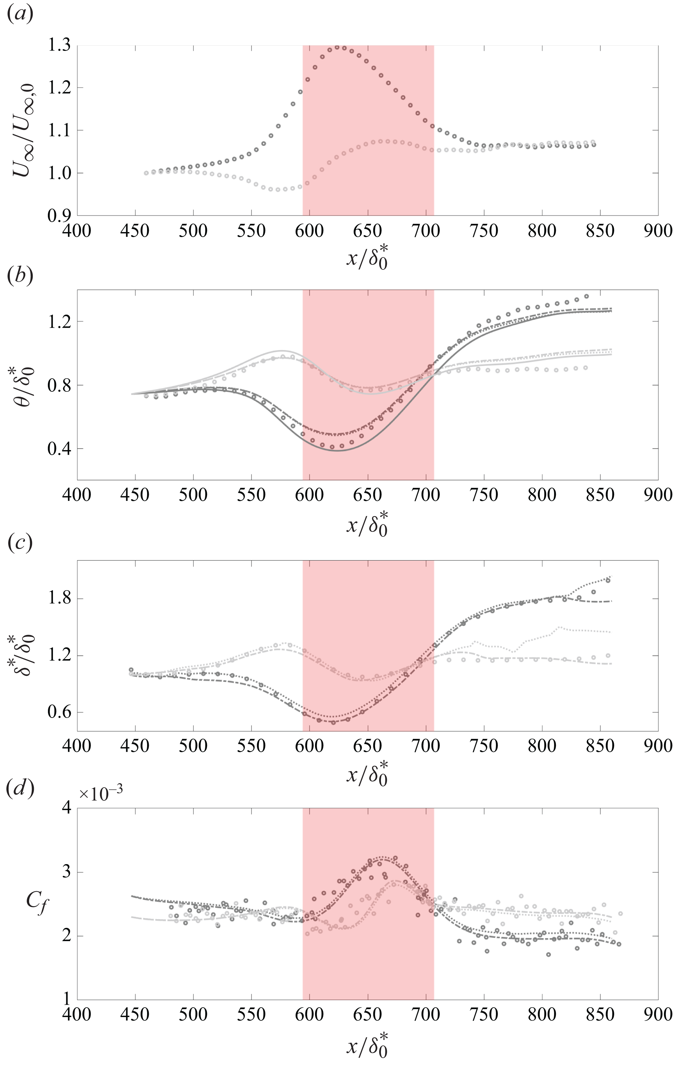
Figure 9. Boundary conditions to the solver and predicted parameters: (a) dimensionless free stream velocity generated underneath the NACA0012 profile; (b) dimensionless momentum thickness; (c) dimensionless displacement thickness; (d) skin friction coefficient; circles, measurements; solid line, prediction by the model in Agrawal et al. (Reference Agrawal, Bose, Griffin and Moin2024); dotted lines, solver defined in the 2-D space; dashed bold lines, solver defined in the 3-D space; gradients of grey from light to dark, AOA = $4^{\circ }$
,
$4^{\circ }$
, $-4^{\circ }$
; light-red box, region below the airfoil at AOA = 0
$-4^{\circ }$
; light-red box, region below the airfoil at AOA = 0 $^\circ$
.
$^\circ$
.
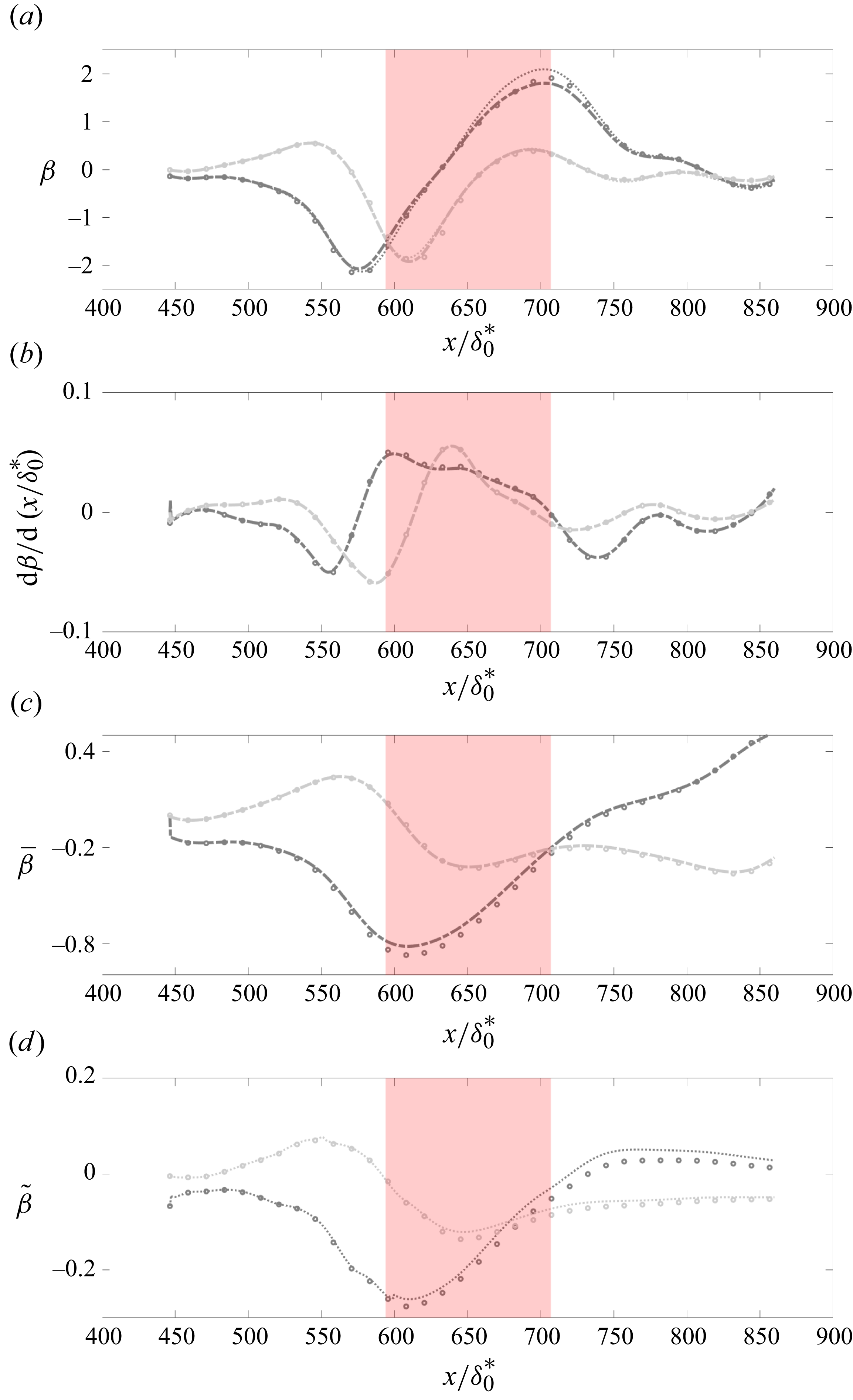
Figure 10. Comparison between calibrated solver and experiments: (a) Clauser parameter $\beta$
; (b) streamwise derivative of
$\beta$
; (b) streamwise derivative of $\beta$
; (c) integral version of
$\beta$
; (c) integral version of $\beta$
according to (A1); (d) integral version of
$\beta$
according to (A1); (d) integral version of $\beta$
according to (A3); circles, experiments; dotted lines, solver defined in the 2-D space; dashed bold lines, solver defined in the 3-D space; gradients of grey from light to dark, AOA =
$\beta$
according to (A3); circles, experiments; dotted lines, solver defined in the 2-D space; dashed bold lines, solver defined in the 3-D space; gradients of grey from light to dark, AOA = $4^{\circ }$
,
$4^{\circ }$
, $-4^{\circ }$
; light-red box, region below the airfoil at AOA = 0
$-4^{\circ }$
; light-red box, region below the airfoil at AOA = 0 $^\circ$
.
$^\circ$
.
4.3. Validation with other datasets
Bobke et al. (Reference Bobke, Vinuesa, Örlü and Schlatter2017) performed LES over a flat plate to assess the effects of different evolutions of $\beta$
(history effects) on velocity profiles, skin friction, integral parameters and turbulence statistics. Their
$\beta$
(history effects) on velocity profiles, skin friction, integral parameters and turbulence statistics. Their $\beta$
profiles exhibit an initial rapid change (for
$\beta$
profiles exhibit an initial rapid change (for $x/\delta ^*_0 \lt 50$
) followed by a nearly constant value over specific streamwise extents. This dataset is utilized to validate the extension of the proposed models. The datasets under consideration are labelled b1 and b2 in Bobke et al. (Reference Bobke, Vinuesa, Örlü and Schlatter2017), corresponding to
$x/\delta ^*_0 \lt 50$
) followed by a nearly constant value over specific streamwise extents. This dataset is utilized to validate the extension of the proposed models. The datasets under consideration are labelled b1 and b2 in Bobke et al. (Reference Bobke, Vinuesa, Örlü and Schlatter2017), corresponding to $\beta = 1$
and
$\beta = 1$
and $\beta = 2$
, respectively, with nearly constant values in the range
$\beta = 2$
, respectively, with nearly constant values in the range $\textit{Re}_\theta$
between 900 and 4000.
$\textit{Re}_\theta$
between 900 and 4000.
Figure 11 presents a comparison between the LES data and the predictions from the solver defined in the 3-D space where the prediction calculations were started at $x/\delta ^*_0 \approx 50$
as the starting point for the space-marching algorithm. Figures 11(a) and 11(c) show the BCs imposed on the model (note that the entire history from the LES data are shown, however, only the region from
$x/\delta ^*_0 \approx 50$
as the starting point for the space-marching algorithm. Figures 11(a) and 11(c) show the BCs imposed on the model (note that the entire history from the LES data are shown, however, only the region from $x/\delta ^*_0 \geq 50$
is used for the predictions). The results show that the model demonstrates excellent agreement with the LES results validating the model’s applicability under these conditions. However, if the calculations were started at
$x/\delta ^*_0 \geq 50$
is used for the predictions). The results show that the model demonstrates excellent agreement with the LES results validating the model’s applicability under these conditions. However, if the calculations were started at $x/\delta ^*_0 \approx 5$
, then the model does not accurately predict the values of
$x/\delta ^*_0 \approx 5$
, then the model does not accurately predict the values of $\beta$
and its integral form,
$\beta$
and its integral form, $\overline {\beta }$
(see figure 11
b,d for
$\overline {\beta }$
(see figure 11
b,d for $5 \leq x/\delta ^*_0 \leq 20$
). In fact, the results suggest that the overall shape of the distributions is captured but rapid changes in
$5 \leq x/\delta ^*_0 \leq 20$
). In fact, the results suggest that the overall shape of the distributions is captured but rapid changes in $\beta$
are not really captured by the current model. This is related to the lack of sufficient training data for
$\beta$
are not really captured by the current model. This is related to the lack of sufficient training data for $d\beta /{\rm d}x$
. Therefore, further work is required to capture the effects of rapidly changing PGs. Having said that, the model parameters (
$d\beta /{\rm d}x$
. Therefore, further work is required to capture the effects of rapidly changing PGs. Having said that, the model parameters ( $A$
and
$A$
and $B$
) could be recalibrated to capture these high PGs and their effects.
$B$
) could be recalibrated to capture these high PGs and their effects.
It is now clear that the proposed model provides reasonable predictions for almost all integral quantities as long as there are no rapid changes in PG histories. With this model at hand, it might now be possible to explore different PG history and its effects on integral quantities. The goal here would be to develop some understanding on the effect of the spatial frequency of PG histories to the boundary layer flow. This is explored in the next section.
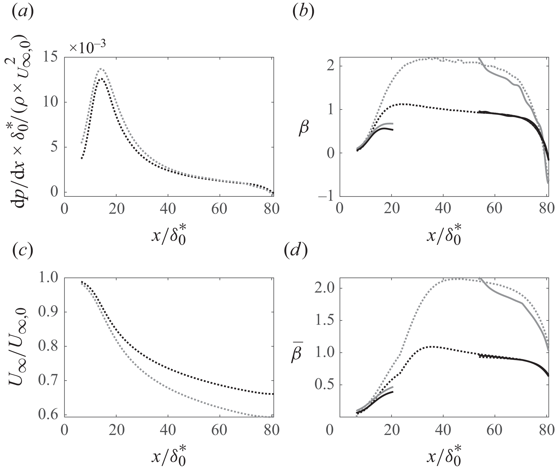
Figure 11. Application of the model to a quasiequilibrium TBL ( $\beta ={\rm constant}$
) simulated with LES from Bobke et al. (Reference Bobke, Vinuesa, Örlü and Schlatter2017). The model is calibrated with the flow developing underneath a NACA0012 profile. The solver starts at
$\beta ={\rm constant}$
) simulated with LES from Bobke et al. (Reference Bobke, Vinuesa, Örlü and Schlatter2017). The model is calibrated with the flow developing underneath a NACA0012 profile. The solver starts at $x/\delta ^*_0=5$
and
$x/\delta ^*_0=5$
and $50$
: (a) dimensionless PG; (b) Clauser parameter; (c) dimensionless free stream velocity; (d), integral version of
$50$
: (a) dimensionless PG; (b) Clauser parameter; (c) dimensionless free stream velocity; (d), integral version of $\beta$
; solid lines, proposed model; dotted lines, Bobke et al. (Reference Bobke, Vinuesa, Örlü and Schlatter2017); black,
$\beta$
; solid lines, proposed model; dotted lines, Bobke et al. (Reference Bobke, Vinuesa, Örlü and Schlatter2017); black, $b1$
simulations (
$b1$
simulations ( $\beta =1$
); grey,
$\beta =1$
); grey, $b2$
simulations (
$b2$
simulations ( $\beta =2$
).
$\beta =2$
).
5. Response of a TBL to imposed PG histories
In § 2, the experimental data presented allow us to observe the behaviour of the TBL under varying PG distributions, which serve as BCs imposed on the developing boundary layer. From these observations, it can be inferred that the evolution of the TBL is particularly influenced by the history of the PG. Specifically, the state of the TBL at a given streamwise location $ x^{\prime}_b$
depends on the entire PG distribution for
$ x^{\prime}_b$
depends on the entire PG distribution for $ x^{\prime} \leq x^{\prime}_b$
. This suggests the use of lag differential equations, where the equation coefficients depend not only on local values of PG and its gradient but also on an integral parameter. This term is defined as a weighted average of PG, providing a means to quantify the history of the PG. This approach forms the basis of the model described in § 3. In § 4, the ODE-based model is first calibrated and then validated for both non-equilibrium and near-equilibrium cases. Once the model is defined, calibrated and validated, we extend its application to a Fourier analysis to derive meaningful insights into the physical behaviour of certain parameters governing the TBL evolution.
$ x^{\prime} \leq x^{\prime}_b$
. This suggests the use of lag differential equations, where the equation coefficients depend not only on local values of PG and its gradient but also on an integral parameter. This term is defined as a weighted average of PG, providing a means to quantify the history of the PG. This approach forms the basis of the model described in § 3. In § 4, the ODE-based model is first calibrated and then validated for both non-equilibrium and near-equilibrium cases. Once the model is defined, calibrated and validated, we extend its application to a Fourier analysis to derive meaningful insights into the physical behaviour of certain parameters governing the TBL evolution.
5.1. Spatial-frequency response of the system
The TBL under different PGs can be conceptualized as a single-input–multiple-output system. The input in this context is the PG distribution, $ {{\rm d}p(x)}/{{\rm d}x}$
, which can be chosen as a sinusoidal function with varying spatial frequencies, see figure 12(a). In this figure, the gradient from light to dark grey represents increasing spatial frequencies of the input sinusoidal function defining
$ {{\rm d}p(x)}/{{\rm d}x}$
, which can be chosen as a sinusoidal function with varying spatial frequencies, see figure 12(a). In this figure, the gradient from light to dark grey represents increasing spatial frequencies of the input sinusoidal function defining $({{\rm d}p}/{{\rm d}x})$
. These histories are not as rapid as those shown in the previous section and therefore the proposed model should be able to capture their effects. By applying such sinusoidal PG distributions, the response of the system can be evaluated to perform a frequency analysis. The frequency used in this analysis is a spatial frequency defined as multiples of
$({{\rm d}p}/{{\rm d}x})$
. These histories are not as rapid as those shown in the previous section and therefore the proposed model should be able to capture their effects. By applying such sinusoidal PG distributions, the response of the system can be evaluated to perform a frequency analysis. The frequency used in this analysis is a spatial frequency defined as multiples of $\omega _0 = 2\pi /L^{\prime}$
, where
$\omega _0 = 2\pi /L^{\prime}$
, where $L^{\prime}$
represents the length of the region of interest over which the TBL develops. For this study,
$L^{\prime}$
represents the length of the region of interest over which the TBL develops. For this study, $L^{\prime}$
is set to
$L^{\prime}$
is set to $400\delta _0^*$
. The PG input is equivalent to having a free stream velocity profile modulated by waves that span the region of interest (see figure 12
c). As
$400\delta _0^*$
. The PG input is equivalent to having a free stream velocity profile modulated by waves that span the region of interest (see figure 12
c). As $ x/\delta ^*_0$
increases, the amplitude of the oscillations in the PG parameter
$ x/\delta ^*_0$
increases, the amplitude of the oscillations in the PG parameter $ \beta$
also increases (see figure 12
b), indicating that gradients progressively exert a stronger influence compared with shear forces. Remarkably, the oscillations in
$ \beta$
also increases (see figure 12
b), indicating that gradients progressively exert a stronger influence compared with shear forces. Remarkably, the oscillations in $ \beta$
remain bounded by consistent envelopes, regardless of the frequency. The parameter
$ \beta$
remain bounded by consistent envelopes, regardless of the frequency. The parameter $ \widetilde {\beta }$
is introduced to represent the cumulative effects of the PGs, weighted according to (A3). As the frequency of
$ \widetilde {\beta }$
is introduced to represent the cumulative effects of the PGs, weighted according to (A3). As the frequency of $ ({{\rm d}p}/{{\rm d}x})$
increases,
$ ({{\rm d}p}/{{\rm d}x})$
increases, $ \widetilde {\beta }$
(see figure 12
d) reaches the same maximum amplitude (
$ \widetilde {\beta }$
(see figure 12
d) reaches the same maximum amplitude ( $\widetilde {\beta } \approx -0.075$
); however, the wavelength of the oscillations decreases with higher frequencies. Hence, the damping effect on the
$\widetilde {\beta } \approx -0.075$
); however, the wavelength of the oscillations decreases with higher frequencies. Hence, the damping effect on the $\widetilde {\beta }$
oscillations increases with higher input frequencies. This implies that spatial high-frequency oscillations in
$\widetilde {\beta }$
oscillations increases with higher input frequencies. This implies that spatial high-frequency oscillations in $ ({{\rm d}p}/{{\rm d}x})$
propagate over shorter spatial regions, effectively localizing the history effects to a smaller area (see figure 12
d).
$ ({{\rm d}p}/{{\rm d}x})$
propagate over shorter spatial regions, effectively localizing the history effects to a smaller area (see figure 12
d).
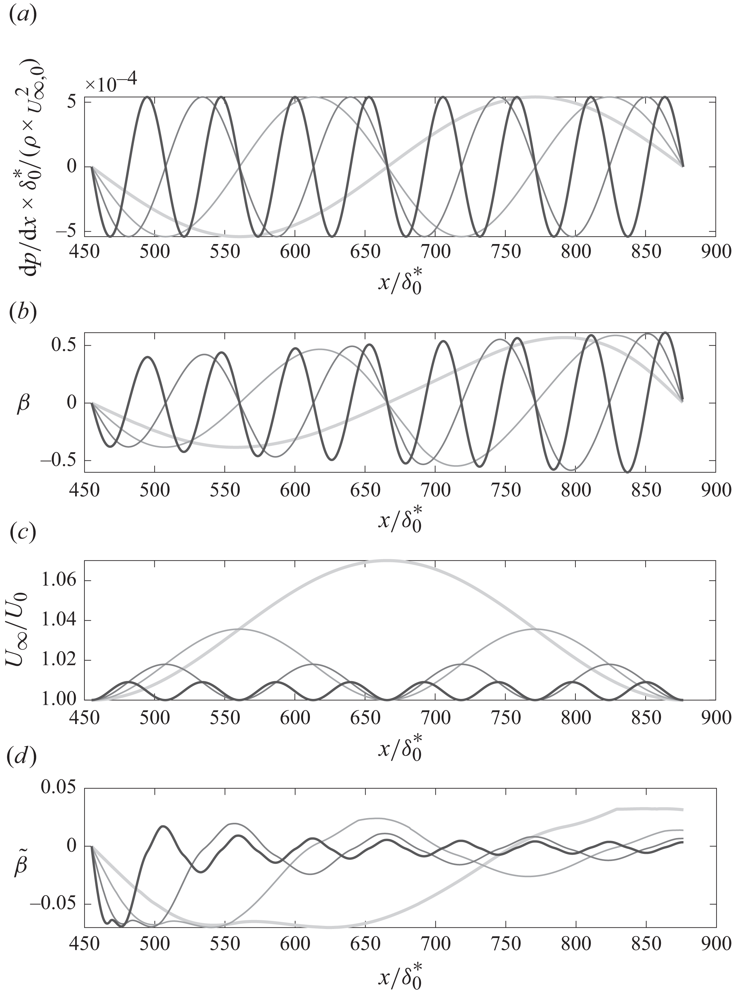
Figure 12. Frequency response of the streamwise evolution of the Clauser parameter and PG history: (a) dimensionless PG; (b) Clauser PG parameter; (c) dimensionless free stream velocity; (d) integral version of $\beta$
; gradients of grey from lighter to darker,
$\beta$
; gradients of grey from lighter to darker, $\omega _0,\ 2\times \omega _0,\ 4\times \omega _0, \ 8\times \omega _0 \ (\omega _0 = 2\pi /L^{\prime}, L^{\prime}=400\delta ^*_0$
).
$\omega _0,\ 2\times \omega _0,\ 4\times \omega _0, \ 8\times \omega _0 \ (\omega _0 = 2\pi /L^{\prime}, L^{\prime}=400\delta ^*_0$
).
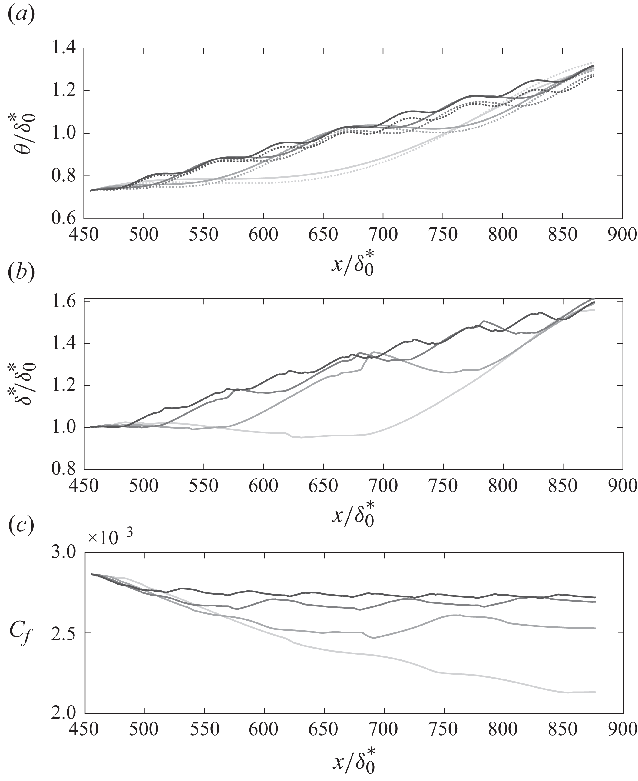
Figure 13. Frequency response of the streamwise evolution of: (a) dimensionless momentum thickness; (b) dimensionless displacement thickness; (c) skin friction coefficient; gradients of grey from lighter to darker, $\omega _0,\ 2\times \omega _0,\ 4\times \omega _0, \ 8\times \omega _0 \ (\omega _0 = 2\pi /L^{\prime}, L^{\prime}=400\delta ^*_0$
); solid lines, proposed model; dotted lines, prediction from Agrawal et al. (Reference Agrawal, Bose, Griffin and Moin2024).
$\omega _0,\ 2\times \omega _0,\ 4\times \omega _0, \ 8\times \omega _0 \ (\omega _0 = 2\pi /L^{\prime}, L^{\prime}=400\delta ^*_0$
); solid lines, proposed model; dotted lines, prediction from Agrawal et al. (Reference Agrawal, Bose, Griffin and Moin2024).
Figure 13 shows the corresponding predictions of skin friction, displacement and momentum thicknesses at different PG frequencies, related to the predicted Clauser parameter (see figure 12
b). The predicted momentum thickness (see figure 13
a) matches the values modelled by Agrawal et al. (Reference Agrawal, Bose, Griffin and Moin2024) for all input spatial frequencies. The displacement thickness (see figure 13
b) follows trends similar to those of $\theta$
due to their connection through the shape factor (as in figure 6
c). The skin friction coefficient (see figure 13
c) exhibits milder variations as the spatial frequency of
$\theta$
due to their connection through the shape factor (as in figure 6
c). The skin friction coefficient (see figure 13
c) exhibits milder variations as the spatial frequency of $({{\rm d}p}/{{\rm d}x})$
increases, which can be attributed to the reduction in free stream velocity fluctuations (see figure 12
c).
$({{\rm d}p}/{{\rm d}x})$
increases, which can be attributed to the reduction in free stream velocity fluctuations (see figure 12
c).
From these observations, it can be inferred that both $ \beta$
and
$ \beta$
and $ \widetilde {\beta }$
exhibit behaviour analogous to sinusoidally driven underdamped oscillators, underscoring the dynamic response of the TBL to PG variations, being described by the second-order differential equation governing mass–spring systems with damping friction and subjected to external forces (Dekker Reference Dekker1977),
$ \widetilde {\beta }$
exhibit behaviour analogous to sinusoidally driven underdamped oscillators, underscoring the dynamic response of the TBL to PG variations, being described by the second-order differential equation governing mass–spring systems with damping friction and subjected to external forces (Dekker Reference Dekker1977),
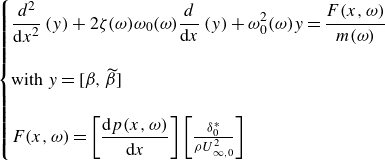 \begin{equation} \begin{cases} \displaystyle \frac {d^2}{{\rm d}x^2}\left (y \right)+2\zeta (\omega)\omega _0(\omega) \frac {d}{{\rm d}x}\left (y\right)+\omega _0^2(\omega)y=\frac {F(x,\omega)}{m(\omega)}\\ \\ \text{with }y = [\beta, \widetilde {\beta }]\\ \\ F(x,\omega) = \left [\displaystyle \frac {{\rm d}p(x,\omega)}{{\rm d}x}\right] \left [\frac {\delta ^*_0}{\rho U_{\infty,0}^2}\right] \end{cases} \end{equation}
with $\zeta$
,
$\zeta$
, $\omega _0$
and
$\omega _0$
and $m$
being, respectively, the damping ratio, natural frequency and mass of an equivalent under-damped spring–mass oscillatory system, and
$m$
being, respectively, the damping ratio, natural frequency and mass of an equivalent under-damped spring–mass oscillatory system, and $\omega$
is the frequency of the forcing input
$\omega$
is the frequency of the forcing input $F(x)$
. From a physical perspective, the newly introduced parameter
$F(x)$
. From a physical perspective, the newly introduced parameter $\widetilde {\beta }$
, an integral form of
$\widetilde {\beta }$
, an integral form of $\beta$
that quantifies the effects of PG history, behaves as a modulated damped harmonic oscillator when a TBL is subjected to sinusoidal BCs. The cumulative effects of PG history are estimated by the calibrated model and follow a distinct harmonic response. The novelty lies in the observation of this behaviour of
$\beta$
that quantifies the effects of PG history, behaves as a modulated damped harmonic oscillator when a TBL is subjected to sinusoidal BCs. The cumulative effects of PG history are estimated by the calibrated model and follow a distinct harmonic response. The novelty lies in the observation of this behaviour of $\beta$
and
$\beta$
and $\widetilde {\beta }$
. The transfer function of the system at a specific frequency
$\widetilde {\beta }$
. The transfer function of the system at a specific frequency $\omega$
is obtained with a Laplace transform of the second-order ODE in (5.1),
$\omega$
is obtained with a Laplace transform of the second-order ODE in (5.1),
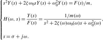 \begin{equation} \begin{cases} s^2Y(s)+2\zeta \omega _0sY(s)+\omega ^2_0Y(s) = F(s)/m,\\ \\ H(\omega,s) = \displaystyle \frac {Y(s)}{F(s)} = \frac {1/m(\omega)}{s^2+2\zeta (\omega) \omega _0(\omega)s+\omega _0^2(\omega)}, \\ \\ s = \sigma +j\omega. \end{cases} \end{equation}
The solution to the second-order ODE in (5.1) is fitted to the output values in figure 12(b,d) to retrieve the values for the damping ratio, natural frequency and mass of the system. Therefore, the frequency response follows the equations at a fixed input frequency $\omega =4\times \omega _0$
,
$\omega =4\times \omega _0$
,
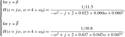 \begin{equation} \begin{cases} \text{for $y$ = $\beta $}\\ H(s=j\omega,\omega =4\times \omega _0) = \displaystyle \frac {1/11.5}{-\omega ^2-j\times 2\times 0.023\times 0.060\omega +0.060^2},\\ \\ \text{for $y$ = $\widetilde {\beta }$}\\ H(s=j\omega,\omega =4\times \omega _0) = \displaystyle \frac {1/10.8}{-\omega ^2+j\times 2\times 0.617\times 0.047\omega +0.047^2}. \end{cases} \end{equation}
The same procedure can be applied at different frequencies to obtain complex numbers that encapsulate information about both the damping and amplification of responses, represented in terms of $\beta$
and
$\beta$
and $\widetilde {\beta }$
as shown in figure 12. The algebraic expressions in (5.3) illustrate the complexities of the differential equations in (3.7) and (3.8) by analysing the frequency-dependent behaviour of the Clauser parameter and the effects of PG history in a developing non-equilibrium TBL. These results are derived from the model presented here. More specifically, (5.3) quantifies
$\widetilde {\beta }$
as shown in figure 12. The algebraic expressions in (5.3) illustrate the complexities of the differential equations in (3.7) and (3.8) by analysing the frequency-dependent behaviour of the Clauser parameter and the effects of PG history in a developing non-equilibrium TBL. These results are derived from the model presented here. More specifically, (5.3) quantifies $H$
, the transfer function of the TBL under sinusoidal streamwise PGs. For a given
$H$
, the transfer function of the TBL under sinusoidal streamwise PGs. For a given $({{\rm d}p}/{{\rm d}x})$
,
$({{\rm d}p}/{{\rm d}x})$
, $H$
determines the corresponding output distribution
$H$
determines the corresponding output distribution $y$
, which can be either
$y$
, which can be either $\beta$
or its integral form, capturing PG history effects. A general PG distribution over the streamwise direction can be decomposed into
$\beta$
or its integral form, capturing PG history effects. A general PG distribution over the streamwise direction can be decomposed into $N$
sinusoidal components, each influencing the TBL through its respective
$N$
sinusoidal components, each influencing the TBL through its respective $H$
. This allows experimentalists to estimate
$H$
. This allows experimentalists to estimate $\beta$
in wind tunnel experiments, improving the design of experiments.
$\beta$
in wind tunnel experiments, improving the design of experiments.
Another input parameter in the chosen PG distribution $({{\rm d}p}/{{\rm d}x})$
that might have an impact on the predictions is the amplitude (
$({{\rm d}p}/{{\rm d}x})$
that might have an impact on the predictions is the amplitude ( $A$
) of the PG modulation. To study this effect, increasing values of
$A$
) of the PG modulation. To study this effect, increasing values of $A$
are set as inputs to the model in figure 14(a) at a spatial frequency of
$A$
are set as inputs to the model in figure 14(a) at a spatial frequency of $\omega = 2\omega _0$
. Figures 14(b) and 14(c) show that
$\omega = 2\omega _0$
. Figures 14(b) and 14(c) show that $\beta$
and
$\beta$
and $\widetilde {\beta }$
still behave as damped harmonic oscillators, with the only effect being on the amplitude of the fluctuations. Therefore, the change in amplitude does not impact the nature of the mass–spring behaviour of the TBL response in the Clauser parameter
$\widetilde {\beta }$
still behave as damped harmonic oscillators, with the only effect being on the amplitude of the fluctuations. Therefore, the change in amplitude does not impact the nature of the mass–spring behaviour of the TBL response in the Clauser parameter $\beta$
nor in the parameter quantifying the history effects of the TBL; it merely amplifies or attenuates the magnitude of the fluctuations. Nevertheless, further simulations and experiments are necessary to explore and validate this linear behaviour of the system, with
$\beta$
nor in the parameter quantifying the history effects of the TBL; it merely amplifies or attenuates the magnitude of the fluctuations. Nevertheless, further simulations and experiments are necessary to explore and validate this linear behaviour of the system, with $\beta$
and
$\beta$
and $\widetilde {\beta }$
serving as outputs. The goal of this analysis is to establish a foundation for a novel approach to characterizing the behaviour of non-equilibrium TBLs under arbitrary PGs and/or spatially varying BCs.
$\widetilde {\beta }$
serving as outputs. The goal of this analysis is to establish a foundation for a novel approach to characterizing the behaviour of non-equilibrium TBLs under arbitrary PGs and/or spatially varying BCs.
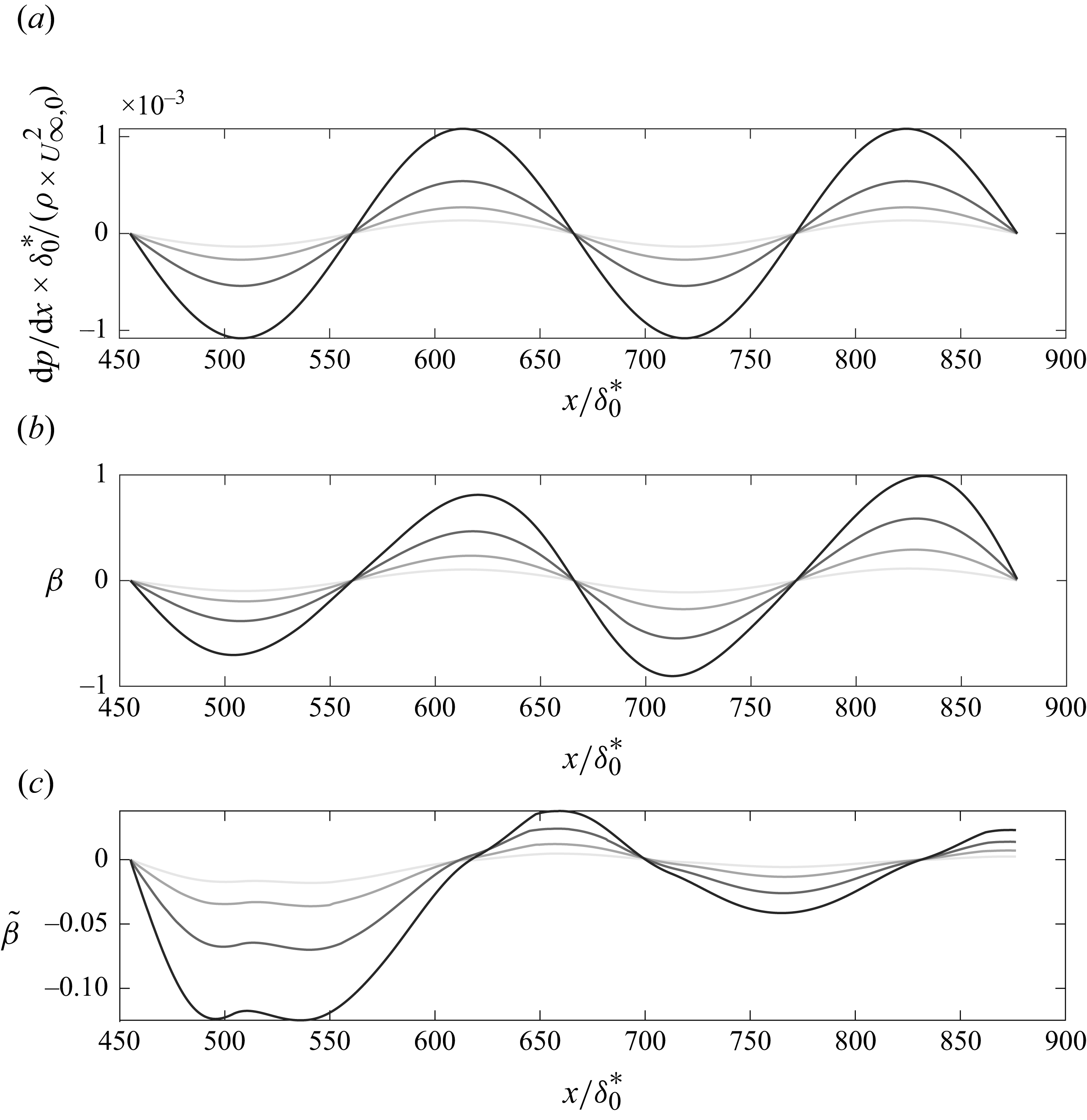
Figure 14. Amplitude effects on the streamwise evolution of the Clauser parameter and PG history: (a) dimensionless PG; (b) Clauser PG parameter; (c) integral version of $\beta$
; greyscale gradient from lighter to darker corresponds to increasing values of
$\beta$
; greyscale gradient from lighter to darker corresponds to increasing values of $ A = 5, 10, 20, 40 \cdot ({\delta _0}/{\rho U_{\infty }^2})$
, where
$ A = 5, 10, 20, 40 \cdot ({\delta _0}/{\rho U_{\infty }^2})$
, where $ A$
represents the amplitude of the
$ A$
represents the amplitude of the $ ({{\rm d}p}/{{\rm d}x})$
sinusoids with spatial frequency
$ ({{\rm d}p}/{{\rm d}x})$
sinusoids with spatial frequency $ 2\omega _0$
.
$ 2\omega _0$
.
6. Conclusions
In this work, we propose a closure system that assists the von Kármán momentum integral equation with two ODEs describing the streamwise evolution of skin friction and displacement thickness. This system accounts for the ‘lag’ or ‘delay’ response of TBL integral parameters to PG changes, incorporating cumulative effects of PG histories through calibration with systematic experimental data. These experiments involve observing TBL behaviour under varying PG fields generated by a NACA0012 airfoil with adjustable AOAs. The primary aim is to offer an alternative framework for evaluating non-equilibrium TBLs without assuming mean velocity profiles, relying instead on the hypothesis that the layer’s state is uniquely determined by the local, derivative and integral values of the Clauser parameter, $\beta$
. The solver’s viability is demonstrated through comparisons with developing TBLs under PGs produced by a wing at various AOAs and LES data from Bobke et al. (Reference Bobke, Vinuesa, Örlü and Schlatter2017). The main limitation of the calibrated model proposed in this work is that it is restricted to
$\beta$
. The solver’s viability is demonstrated through comparisons with developing TBLs under PGs produced by a wing at various AOAs and LES data from Bobke et al. (Reference Bobke, Vinuesa, Örlü and Schlatter2017). The main limitation of the calibrated model proposed in this work is that it is restricted to $\beta = [-4, 2.6]$
,
$\beta = [-4, 2.6]$
, ${({\rm d}\beta)}/{({\rm d}(x/\delta ^*_0))}=[-20, 10]$
,
${({\rm d}\beta)}/{({\rm d}(x/\delta ^*_0))}=[-20, 10]$
, $\widetilde {\beta } = [-0.25,0.20]$
and
$\widetilde {\beta } = [-0.25,0.20]$
and $\overline {\beta } = [-1, 1]$
. For flows whose values are beyond these regions, then the model should be recalibrated and validated before further use. The model was used to develop some understanding of the boundary layer response to imposed PG histories within this specified range of parameters. Sinusoidal variations in PG histories were imposed to explore the variations in the flow. Results suggest that the boundary layer behaves as an under-damped oscillator where low-amplitude high-frequency changes in imposed history only have a local effect while low frequency variations are seen to affect larger portions of the flow. Future studies should explore these scenarios in experiments and simulations while using this model for early stage predictions and improving the model further using the obtained data.
$\overline {\beta } = [-1, 1]$
. For flows whose values are beyond these regions, then the model should be recalibrated and validated before further use. The model was used to develop some understanding of the boundary layer response to imposed PG histories within this specified range of parameters. Sinusoidal variations in PG histories were imposed to explore the variations in the flow. Results suggest that the boundary layer behaves as an under-damped oscillator where low-amplitude high-frequency changes in imposed history only have a local effect while low frequency variations are seen to affect larger portions of the flow. Future studies should explore these scenarios in experiments and simulations while using this model for early stage predictions and improving the model further using the obtained data.
It should be noted that the calibrated model presented here lacks full generalization for all developing TBLs under different PGs, particularly those with strong derivatives of $\beta =\beta (x)$
. Specifically, we attempted to predict the integral parameters of a TBL developing in a convergent–divergent wind tunnel (data from Volino et al., (Reference Volino2020)) but the results were unsatisfactory. It remains unclear whether the issue is due to the model’s limited extendibility or the differing parameter ranges involved. Nonetheless, the primary objective of this work is to provide a flexible framework that can be adopted by other researchers to train the model using diverse datasets. To facilitate this, we will share both the code and the training data we used, which can be modified and extended by others. As in Perry et al. (Reference Perry, Marusic and Jones2002), our goal is to offer a set of ODEs with trainable coefficients that can be adapted to various datasets, thereby enhancing the model’s applicability across different contexts.
$\beta =\beta (x)$
. Specifically, we attempted to predict the integral parameters of a TBL developing in a convergent–divergent wind tunnel (data from Volino et al., (Reference Volino2020)) but the results were unsatisfactory. It remains unclear whether the issue is due to the model’s limited extendibility or the differing parameter ranges involved. Nonetheless, the primary objective of this work is to provide a flexible framework that can be adopted by other researchers to train the model using diverse datasets. To facilitate this, we will share both the code and the training data we used, which can be modified and extended by others. As in Perry et al. (Reference Perry, Marusic and Jones2002), our goal is to offer a set of ODEs with trainable coefficients that can be adapted to various datasets, thereby enhancing the model’s applicability across different contexts.
Supplementary material
Data published in this article are available from the University of Southampton repository at https://doi.org/10.5258/SOTON/D3491.
Funding
This work was financially supported by the Engineering and Physical Sciences Research Council (EPSRC) through the grants EP/V05614X/1 and EP/W026090/1.
Declaration of interests
The authors report no conflict of interest.
Appendix A. Pressure gradient history parameters
The coefficients (A and B in (4.1)) of the data-driven models are defined as functions of three parameters that describe the state of the TBL at a given streamwise position $x^{\prime}= x / \delta ^*_0$
: the Clauser PG parameter
$x^{\prime}= x / \delta ^*_0$
: the Clauser PG parameter $ \beta$
, its local derivative
$ \beta$
, its local derivative $ {\rm d}\beta /{\rm d}x^{\prime}$
and an integral form of
$ {\rm d}\beta /{\rm d}x^{\prime}$
and an integral form of $ \beta$
that quantifies the history of the PGs, denoted as
$ \beta$
that quantifies the history of the PGs, denoted as $ \overline {\beta }$
or
$ \overline {\beta }$
or $ \widetilde {\beta }$
. The choice between
$ \widetilde {\beta }$
. The choice between $ \overline {\beta }$
and
$ \overline {\beta }$
and $ \widetilde {\beta }$
depends on the selection of the dimensional parameter space used to define the model. The following subsections describe these parameter spaces and their respective parameters in detail.
$ \widetilde {\beta }$
depends on the selection of the dimensional parameter space used to define the model. The following subsections describe these parameter spaces and their respective parameters in detail.
A.1 The 3-D parameter space
Vinuesa et al. (Reference Vinuesa, Örlü, Sanmiguel Vila, Ianiro, Discetti and Schlatter2017) established criteria to assess whether a TBL in an APG can be considered well-behaved, i.e. independent of the inflow conditions. The term ’well-behaved’ in ZPG flows represents the canonical state. To account for the history effects of ( ${\rm d}p/{\rm d}x^{\prime}$
) in evaluating skin friction in APG cases relative to ZPG cases, they introduced an integral parameter
${\rm d}p/{\rm d}x^{\prime}$
) in evaluating skin friction in APG cases relative to ZPG cases, they introduced an integral parameter $\overline {\beta }$
, which represents a mean value over a range of
$\overline {\beta }$
, which represents a mean value over a range of $\textit{Re}_\theta$
. In computing this average, equal weight is assigned to all values from the onset of the TBL evolution up to a specified
$\textit{Re}_\theta$
. In computing this average, equal weight is assigned to all values from the onset of the TBL evolution up to a specified $\textit{Re}_\theta (x^{\prime}_b)$
. In our approach, we employ a similar averaging method but within a specified streamwise window, highlighting the significance of local
$\textit{Re}_\theta (x^{\prime}_b)$
. In our approach, we employ a similar averaging method but within a specified streamwise window, highlighting the significance of local $\beta$
values in the averaging. Additionally, instead of integrating over
$\beta$
values in the averaging. Additionally, instead of integrating over $\textit{Re}_\theta$
, we perform the integration over
$\textit{Re}_\theta$
, we perform the integration over $x^{\prime}= x / \delta ^*_0$
,
$x^{\prime}= x / \delta ^*_0$
,
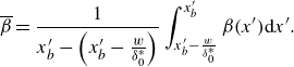 \begin{equation} \overline {\beta } = \displaystyle \frac {1}{ x^{\prime}_b-\left (x^{\prime}_b-\frac {w}{\delta ^*_0}\right)} \int _{x^{\prime}_b-\frac {w}{\delta ^*_0}}^{x^{\prime}_b}{\beta (x^{\prime}) {\rm d}x^{\prime}}. \end{equation}
The integral is computed over a streamwise window of $[x^{\prime}_b-w/\delta ^*_0,x^{\prime}_b]$
. The size of the window
$[x^{\prime}_b-w/\delta ^*_0,x^{\prime}_b]$
. The size of the window $w$
is chosen to minimize the error between the prediction (
$w$
is chosen to minimize the error between the prediction ( $(\ldots)_p$
) and the measure (
$(\ldots)_p$
) and the measure ( $(\ldots)_m$
) of the displacement thickness
$(\ldots)_m$
) of the displacement thickness
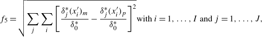 \begin{equation} f_5 = \sqrt {\sum _j\sum _i \left [\frac {\delta ^*_j(x^{\prime}_i)_m}{\delta ^*_0}-\frac {\delta ^*_j(x^{\prime}_i)_p}{\delta ^*_0} \right]^2} \text{with } i=1, \ldots, I \text{ and } j=1, \ldots, J, \end{equation}
where $I$
denotes the number of streamwise points and
$I$
denotes the number of streamwise points and $J$
the number of AOA tested. The optimization algorithm employed for this problem is a genetic algorithm (GA), which identifies the global unconstrained minimum of
$J$
the number of AOA tested. The optimization algorithm employed for this problem is a genetic algorithm (GA), which identifies the global unconstrained minimum of $f_5$
within the bounds
$f_5$
within the bounds $[1, 450]$
for
$[1, 450]$
for $w/\delta ^*_0$
. The GA begins by generating a random initial population and evaluating the corresponding values of
$w/\delta ^*_0$
. The GA begins by generating a random initial population and evaluating the corresponding values of $f_5$
. A selection process retains the best-performing solutions, discarding the rest of the population. Subsequently, the algorithm applies mutation and crossover operators to create a new population. These steps are iteratively repeated until convergence is achieved. The choice of a GA over other optimization routines is justified by two key factors (Verstraete et al. Reference Verstraete, Coletti, Bulle, Vanderwielen and Arts2013). First, the GA performs a global search, reducing the risk of becoming trapped in local minima. Second, it does not require an initial guess, allowing it to converge to an optimal solution without prior assumptions. The 3-D space defined by the values of
$f_5$
. A selection process retains the best-performing solutions, discarding the rest of the population. Subsequently, the algorithm applies mutation and crossover operators to create a new population. These steps are iteratively repeated until convergence is achieved. The choice of a GA over other optimization routines is justified by two key factors (Verstraete et al. Reference Verstraete, Coletti, Bulle, Vanderwielen and Arts2013). First, the GA performs a global search, reducing the risk of becoming trapped in local minima. Second, it does not require an initial guess, allowing it to converge to an optimal solution without prior assumptions. The 3-D space defined by the values of $\beta$
,
$\beta$
, ${\rm d}\beta /{\rm d}x^{\prime}$
and
${\rm d}\beta /{\rm d}x^{\prime}$
and $\overline {\beta }$
along the streamwise locations
$\overline {\beta }$
along the streamwise locations $x$
is shown in figure 15(a) for the five different AOAs under investigation. The development of the TBL under a specific PG imposed by an AOA traces a trajectory in the 3-D parameter space. In the § 4, it is discussed how to extract meaningful information from this dimensional space to predict the streamwise evolution of the boundary layer.
$x$
is shown in figure 15(a) for the five different AOAs under investigation. The development of the TBL under a specific PG imposed by an AOA traces a trajectory in the 3-D parameter space. In the § 4, it is discussed how to extract meaningful information from this dimensional space to predict the streamwise evolution of the boundary layer.
A.2 Reduced-order parameter space
The previous paragraph shows that there is a clear relationship between $\beta$
,
$\beta$
, ${\rm d}\beta /{\rm d}x^{\prime}$
and
${\rm d}\beta /{\rm d}x^{\prime}$
and $\overline {\beta }$
and therefore it may be possible to further reduce these three parameters. We propose a reduced-order space
$\overline {\beta }$
and therefore it may be possible to further reduce these three parameters. We propose a reduced-order space $ (\beta, \widetilde {\beta })$
, where
$ (\beta, \widetilde {\beta })$
, where $ \widetilde {\beta } = f_4(\beta, {\rm d}\beta /{\rm d}x^{\prime}, x^{\prime})$
is an integral parameter that serves as an alternative to
$ \widetilde {\beta } = f_4(\beta, {\rm d}\beta /{\rm d}x^{\prime}, x^{\prime})$
is an integral parameter that serves as an alternative to $ \overline {\beta }$
. Here, the PG history effects is captured as a weighted average of all values of
$ \overline {\beta }$
. Here, the PG history effects is captured as a weighted average of all values of $\beta$
from the start of the evolution (
$\beta$
from the start of the evolution ( $x^{\prime}_0$
) of the TBL up to a specific point
$x^{\prime}_0$
) of the TBL up to a specific point $ x^{\prime}_b$
. Unlike the 3-D case, where a windowing of the integral is used, in this case,
$ x^{\prime}_b$
. Unlike the 3-D case, where a windowing of the integral is used, in this case, $\widetilde {\beta }$
involves a weighting function
$\widetilde {\beta }$
involves a weighting function $ W$
,
$ W$
,
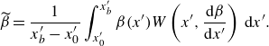 \begin{equation} \widetilde {\beta } = \frac {1}{\displaystyle x^{\prime}_b - x^{\prime}_0} \int _{x^{\prime}_0}^{x^{\prime}_b} \beta ( x^{\prime}) W\left ( x^{\prime}, \frac {{\rm d}\beta }{{\rm d}x^{\prime}} \right) \, {\rm d}x^{\prime}.\end{equation}
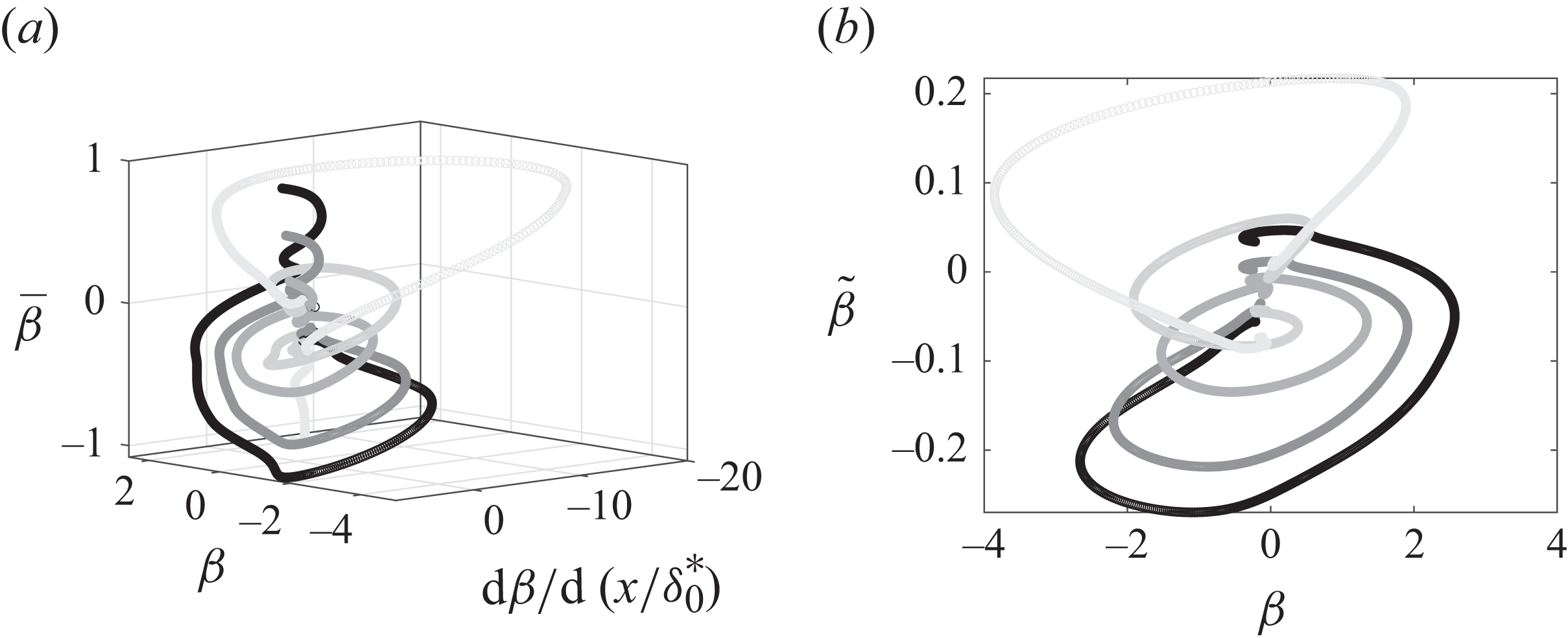
Figure 15. The 3-D and reduced-order domains for TBLs developing under a NACA0012 airfoil: (a) $(\beta, ({{\rm d} \beta }/{{\rm d}(x/\delta ^*_0)}), \overline {\beta })$
is the 3-D space where the flow under investigation is defined; (b)
$(\beta, ({{\rm d} \beta }/{{\rm d}(x/\delta ^*_0)}), \overline {\beta })$
is the 3-D space where the flow under investigation is defined; (b) $(\beta, \widetilde {\beta })$
is the 2-D space where the flow under investigation is defined; gradients of grey from light to dark, AOA =
$(\beta, \widetilde {\beta })$
is the 2-D space where the flow under investigation is defined; gradients of grey from light to dark, AOA = $8^{\circ }$
,
$8^{\circ }$
, $4^{\circ }$
,
$4^{\circ }$
, $0^{\circ }$
,
$0^{\circ }$
, $-4^{\circ }$
,
$-4^{\circ }$
, $-8^{\circ }$
.
$-8^{\circ }$
.
The weighting is a 2-D sigmoid function, which assigns different weights to the values of $\beta$
within the range
$\beta$
within the range $[x^{\prime}_0, x^{\prime}_b]$
, depending on their streamwise distance from
$[x^{\prime}_0, x^{\prime}_b]$
, depending on their streamwise distance from $x^{\prime}_b$
and the local gradient of
$x^{\prime}_b$
and the local gradient of $\beta$
,
$\beta$
,
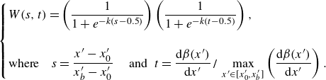 \begin{equation} \begin{cases} W(s,t) = \left ( \displaystyle \frac {1}{1 + e^{-k(s - 0.5)}} \right) \left ( \displaystyle \frac {1}{1 + e^{-k(t - 0.5)}} \right), \\ \\ \text{where} \quad s = \displaystyle \frac { x^{\prime} - x^{\prime}_0}{x^{\prime}_b - x^{\prime}_0}\quad \textrm { and}\,\,\,t = \displaystyle \frac {{\rm d}\beta (x^{\prime})}{{\rm d}x^{\prime}} \, \Bigg / \, \max _{ x^{\prime} \in [x^{\prime}_0, x^{\prime}_b]} \left (\frac {{\rm d}\beta ( x^{\prime})}{{\rm d}x^{\prime}}\right). \end{cases} \end{equation}
In general, the 1-D sigmoid function is used in weighting for its smooth, continuous transition between 0 and 1, with an adjustable steepness controlled by the parameter $ k$
, allowing for gradual or more abrupt changes. The
$ k$
, allowing for gradual or more abrupt changes. The $ -0.5$
shift centres the curve around
$ -0.5$
shift centres the curve around $ s \text{ or } t = 0.5$
, ensuring a smooth transition from values close to 0 at
$ s \text{ or } t = 0.5$
, ensuring a smooth transition from values close to 0 at $ s \text{ or } t = 0$
to values close to unity at
$ s \text{ or } t = 0$
to values close to unity at $ s \text{ or } t = 1$
. The 2-D shifted sigmoid function satisfies the ideal conditions
$ s \text{ or } t = 1$
. The 2-D shifted sigmoid function satisfies the ideal conditions $ W(s=0, t=0) = 0$
and
$ W(s=0, t=0) = 0$
and $ W(s=1, t=1) = 1$
, particularly for
$ W(s=1, t=1) = 1$
, particularly for $ k \gg 1$
. The value of
$ k \gg 1$
. The value of $ k$
in (A4) is determined similarly to
$ k$
in (A4) is determined similarly to $ w$
(A1) using a GA which finds the optimum in the range
$ w$
(A1) using a GA which finds the optimum in the range $[0.1, 5]$
. The 2-D space defined by and
$[0.1, 5]$
. The 2-D space defined by and $\widetilde {\beta }$
along the streamwise locations
$\widetilde {\beta }$
along the streamwise locations $x^{\prime}$
is shown in figure 15(b) for the five different AOAs under investigation.
$x^{\prime}$
is shown in figure 15(b) for the five different AOAs under investigation.


 Open access