


1. Introduction
The radio evolution of core-collapse supernovae (SNe) years to decades after the explosion is a function both of the last stages of evolution of the progenitor star, and of the energy and geometry of the explosion and associated mass ejection. However, the modelling of such processes is hampered by the scarcity of observational constraints; that is, few SNe have been followed in the radio bands both at early and late times. Typical radio light curves are well modelled (Chevalier Reference Chevalier1982b; Weiler et al. Reference Weiler, Sramek, Panagia, van der Hulst and Salvati1986, Reference Weiler, Panagia, Montes and Sramek2002; Sramek & Weiler Reference Sramek, Weiler and Weiler2003; Chevalier, Fransson, & Nymark Reference Chevalier, Fransson and Nymark2006; Chevalier & Fransson Reference Chevalier and Fransson2006) by an initial flux increase, over the first few weeks or months; this rise is caused by a decrease of the optical depth of absorbing material in the circumstellar medium (CSM), as the synchrotron-emitting blast wave expands. The peak is reached first at shorter wavelengths, then at longer wavelengths. After the source becomes optically thin at a given frequency, its flux density at that frequency declines (as a first approximation) as a power-law. When the emission is optically thin at all frequencies, the spectral index $\alpha$
(defined as
$\alpha$
(defined as $F_\nu \propto \nu^{\alpha}$
) has been observed to approach an asymptotically constant, negative value, typically
$F_\nu \propto \nu^{\alpha}$
) has been observed to approach an asymptotically constant, negative value, typically $-1 \lesssim \alpha \lesssim -0.5$
(Weiler et al. Reference Weiler, Sramek, Panagia, van der Hulst and Salvati1986; Weiler, Panagia, & Sramek Reference Weiler, Panagia and Sramek1990).
$-1 \lesssim \alpha \lesssim -0.5$
(Weiler et al. Reference Weiler, Sramek, Panagia, van der Hulst and Salvati1986; Weiler, Panagia, & Sramek Reference Weiler, Panagia and Sramek1990).
In recent years, observational studies of a few decades-old SNe have suggested late-time deviations from the power-law decline. In some sources, the flux drops abruptly and exponentially after a few years; the Type IIb SN 1993J (Weiler et al. Reference Weiler, Williams, Panagia, Stockdale, Kelley, Sramek, Van Dyk and Marcaide2007) in M81 and the Type IIb SN 2001gd (Stockdale et al. Reference Stockdale and Williams2007) are well-studied examples of such behaviour. A possible interpretation of such an evolution is that the blast wave has overtaken the dense, slow wind from the red-supergiant progenitor and has reached the lower-density interstellar medium. In other (more numerous) sources, instead, a radio re-brightening (sometimes accompanied by X-ray re-brightening) is observed after a few years (Wellons, Soderberg, & Chevalier Reference Wellons, Soderberg and Chevalier2012; Chevalier & Fransson Reference Chevalier, Fransson, Alsabti and Murdin2017; Stroh et al. Reference Stroh2021; Rose et al. Reference Rose2024). Notable examples of radio re-brightenings include the Type II-peculiar SN 1987A (Cendes et al. Reference Cendes, Gaensler, Ng, Zanardo, Staveley-Smith and Tzioumis2018) in the Large Magellanic Cloud, the Type IIn SN 1996cr (Meunier et al. Reference Meunier, Bauer, Dwarkadas, Koribalski, Emonts, Hunstead, Campbell-Wilson, Stockdale and Tingay2013) in the Circinus galaxy, the Type Ib SN 2014C (Margutti et al. Reference Margutti2017) in NGC 7331, the Type IIb SN 2003bg in MCG 05-10-15 (Rose et al. Reference Rose2024) and the Type IIL SN 2018ivc (Maeda et al. Reference Maeda, Michiyama, Chandra, Ryder, Kuncarayakti, Hiramatsu and Imanishi2023) in NGC 1068.
At least three alternative scenarios have been invoked to explain re-brightenings in decades-old SNe. It could be due to a denser and clumpier circumstellar shell encountered by the expanding shock wave (Chevalier Reference Chevalier1998; Chevalier & Fransson Reference Chevalier, Fransson, Alsabti and Murdin2017; Margutti et al. Reference Margutti2017). Alternatively, it could be the signature of an off-axis, relativistic jet that is becoming less collimated over time and is entering our line of sight (Paczynski Reference Paczynski2001; Granot et al. Reference Granot, Panaitescu, Kumar and Woosley2002). Thirdly, it could be the emergence of a pulsar wind nebula (Slane Reference Slane, Alsabti and Murdin2017) powered by the newborn neutron star.
Monitoring the long-term evolution of the radio emission is particularly important in the case of Type IIb SNe, for which the mass and evolutionary stage of their progenitors is still actively debated (Sravan, Marchant, & Kalogera Reference Sravan, Marchant and Kalogera2019; Sravan et al. Reference Sravan, Marchant, Kalogera, Milisavljevic and Margutti2020). Type IIb SNe initially show evidence for hydrogen emission that soon subsides, within a few days after explosion. After this epoch the SN develops prominent He features similar to Ib SNe (Filippenko Reference Filippenko1988; Nomoto et al. Reference Nomoto, Suzuki, Shigeyama, Kumagai, Yamaoka and Saio1993; Podsiadlowski et al. Reference Podsiadlowski1993; Filippenko Reference Filippenko1997; Dessart et al. Reference Dessart, John Hillier, Livne, Yoon, Woosley, Waldman and Langer2011; Gilkis & Arcavi Reference Gilkis and Arcavi2022). This suggests that Type IIb progenitor stars have retained only a small layer of hydrogen ( $\sim$
0.1 M
$\sim$
0.1 M $_\odot$
) at the final collapse. The most likely reason for the substantial (but not complete) loss of hydrogen is envelope stripping in a binary system (Podsiadlowski et al. Reference Podsiadlowski1993; Claeys et al. Reference Claeys, de Mink, Pols, Eldridge and Baes2011; Sravan et al. Reference Sravan, Marchant, Kalogera, Milisavljevic and Margutti2020). Tentative observational evidence of a surviving binary companion (a B1–B3 supergiant) was indeed proposed for the IIb SN 1993J (Fox et al. Reference Fox2014).
$_\odot$
) at the final collapse. The most likely reason for the substantial (but not complete) loss of hydrogen is envelope stripping in a binary system (Podsiadlowski et al. Reference Podsiadlowski1993; Claeys et al. Reference Claeys, de Mink, Pols, Eldridge and Baes2011; Sravan et al. Reference Sravan, Marchant, Kalogera, Milisavljevic and Margutti2020). Tentative observational evidence of a surviving binary companion (a B1–B3 supergiant) was indeed proposed for the IIb SN 1993J (Fox et al. Reference Fox2014).
The most interesting open question (Chevalier & Soderberg Reference Chevalier and Soderberg2010; Yoon, Dessart, & Clocchiatti Reference Yoon, Dessart and Clocchiatti2017; Sravan, Marchant, & Kalogera Reference Sravan, Marchant and Kalogera2019; Sravan et al. Reference Sravan, Marchant, Kalogera, Milisavljevic and Margutti2020) related to Type IIb SNe is whether their progenitors are extended, such as red or yellow supergiants (easier to detect in pre-explosion optical images: Kamble et al. Reference Kamble2016) or compact, such as stripped stars or Wolf-Rayet stars, similar to Type-Ibc progenitors (not usually detected in pre-explosion images). Extended progenitors have characteristic radii $R_\ast \sim$
10
$R_\ast \sim$
10 $^{13}$
cm and relatively slow wind speeds
$^{13}$
cm and relatively slow wind speeds $v_{w} \sim 10$
–100 km s
$v_{w} \sim 10$
–100 km s $^{-1}$
; compact progenitors have radii
$^{-1}$
; compact progenitors have radii $R_\ast \sim$
10
$R_\ast \sim$
10 $^{11}$
cm, with faster wind speeds
$^{11}$
cm, with faster wind speeds $v_{w} \sim 500$
–1 000 km s
$v_{w} \sim 500$
–1 000 km s $^{-1}$
. The fastest SN ejecta reach speeds of
$^{-1}$
. The fastest SN ejecta reach speeds of $\approx$
10 000–15 000 km s
$\approx$
10 000–15 000 km s $^{-1}$
in extended IIb’s, but as high as
$^{-1}$
in extended IIb’s, but as high as $\approx$
30 000–50 000 km s
$\approx$
30 000–50 000 km s $^{-1}$
in compact IIb events, because the ejecta expand into a faster, thinner progenitor wind (Chevalier & Soderberg Reference Chevalier and Soderberg2010). This difference in the ejecta/CSM interaction, in turn, leads to a different evolution of the radio synchrotron emission, especially in the rise-time versus peak-luminosity plane (Kamble et al. Reference Kamble2016; Stroh et al. Reference Stroh2021). It is also possible that there is a continuum distribution of SN morphologies spanning Ib’s, compact IIb’s and extended IIb’s, rather than separate classes (Chevalier & Soderberg Reference Chevalier and Soderberg2010; Horesh et al. Reference Horesh2013; Stroh et al. Reference Stroh2021).
$^{-1}$
in compact IIb events, because the ejecta expand into a faster, thinner progenitor wind (Chevalier & Soderberg Reference Chevalier and Soderberg2010). This difference in the ejecta/CSM interaction, in turn, leads to a different evolution of the radio synchrotron emission, especially in the rise-time versus peak-luminosity plane (Kamble et al. Reference Kamble2016; Stroh et al. Reference Stroh2021). It is also possible that there is a continuum distribution of SN morphologies spanning Ib’s, compact IIb’s and extended IIb’s, rather than separate classes (Chevalier & Soderberg Reference Chevalier and Soderberg2010; Horesh et al. Reference Horesh2013; Stroh et al. Reference Stroh2021).
Late time radio studies of IIb events can reveal the epoch of hydrogen-envelope removal and the structure of the CSM, and in this way constrain stellar evolution. Well-studied representatives of the extended IIb class are SN 1993J and SN 2001gd (Chevalier & Soderberg Reference Chevalier and Soderberg2010), both of which show late-time drops in their radio emission, as mentioned earlier. The Milky Way SN Cassiopeia A was also an extended IIb event, probably with a red supergiant progenitor (Krause et al. Reference Krause, Birkmann, Usuda, Hattori, Goto, Rieke and Misselt2008), although a Wolf-Rayet phase just before the explosion has also been suggested (Hwang & Laming Reference Hwang and Laming2009). Conversely, SN 2001ig has been interpreted as a compact-progenitor IIb (Ryder et al. Reference Ryder, Sadler, Subrahmanyan, Weiler, Panagia and Stockdale2004, Reference Ryder2018). In this paper, we study the late-time radio evolution of SN 2001ig, to test whether and how it differs from that seen in extended IIb SNe.
2. Early evolution of SN 2001ig
SN 2001ig was discovered by Evans, White, & Bembrick (Reference Evans, White and Bembrick2001)Footnote
a
on 2001 December 10.43 UT, in the face-on spiral galaxy NGC 7424. A likely explosion date is 2001 December 3 (MJD 52246) (Ryder et al. Reference Ryder, Sadler, Subrahmanyan, Weiler, Panagia and Stockdale2004), based on the early radio light curve evolution. Following Soria et al. (Reference Soria, Cheng, Pakull, Motch and Russell2024), we adopt a galaxy distance $d = 10.8$
Mpc (taken as the average between the Hubble Flow distance of 10.1 Mpc and the Tully-Fisher distance of 11.5 Mpc, as reported in the NASA/IPAC Extragalactic Database); this corresponds to a distance modulus of 30.17 mag and a scale of 52 pc arcsec
$d = 10.8$
Mpc (taken as the average between the Hubble Flow distance of 10.1 Mpc and the Tully-Fisher distance of 11.5 Mpc, as reported in the NASA/IPAC Extragalactic Database); this corresponds to a distance modulus of 30.17 mag and a scale of 52 pc arcsec $^{-1}$
. The SN position, determined from Australia Telescope Compact Array (ATCA) maps (Soria et al. Reference Soria, Cheng, Pakull, Motch and Russell2024), is R.A.(J2000)
$^{-1}$
. The SN position, determined from Australia Telescope Compact Array (ATCA) maps (Soria et al. Reference Soria, Cheng, Pakull, Motch and Russell2024), is R.A.(J2000) $= 22^{\rm h}\,57^{\rm m}\,30^{\rm s}.74 (\pm 0{\kern.5pt}.^{{\kern-2.5pt}\prime\prime}04)$
, Dec.(J2000)
$= 22^{\rm h}\,57^{\rm m}\,30^{\rm s}.74 (\pm 0{\kern.5pt}.^{{\kern-2.5pt}\prime\prime}04)$
, Dec.(J2000) $= -41^{\circ}\,02^{\prime}\,26{\kern.5pt}.^{{\kern-2.5pt}\prime\prime}35 (\pm 0{\kern.5pt}.^{{\kern-2.5pt}\prime\prime}05)$
.
$= -41^{\circ}\,02^{\prime}\,26{\kern.5pt}.^{{\kern-2.5pt}\prime\prime}35 (\pm 0{\kern.5pt}.^{{\kern-2.5pt}\prime\prime}05)$
.

Figure 1. 9 GHz ATCA contours (cyan) of SN 2001ig observed on 2024 April 24, overlaid on a Gemini/GMOS colour composite image from 2004 September 13. Contours are defined as $2^{n/2}$
times the local rms noise level, which was
$2^{n/2}$
times the local rms noise level, which was $\approx$
12
$\approx$
12 $\mu$
Jy. The three plotted contours correspond to 68
$\mu$
Jy. The three plotted contours correspond to 68 $\mu$
Jy (5.7
$\mu$
Jy (5.7 $\sigma$
), 96
$\sigma$
), 96 $\mu$
Jy (8
$\mu$
Jy (8 $\sigma$
) and 135
$\sigma$
) and 135 $\mu$
Jy (11.3
$\mu$
Jy (11.3 $\sigma$
). The beam size as shown at lower right was 1
$\sigma$
). The beam size as shown at lower right was 1 ${\kern.5pt}.^{{\kern-2.5pt}\prime\prime}$
6
${\kern.5pt}.^{{\kern-2.5pt}\prime\prime}$
6 $\times$
0
$\times$
0 ${\kern.5pt}.^{{\kern-2.5pt}\prime\prime}$
8 at a position angle (north through east) of 158
${\kern.5pt}.^{{\kern-2.5pt}\prime\prime}$
8 at a position angle (north through east) of 158 ${\kern.5pt}.^{{\kern-2.5pt}\circ}$
0. See Ryder et al. (Reference Ryder, Murrowood and Stathakis2006, Reference Ryder2018) for a discussion on the nature of the optical counterpart.
${\kern.5pt}.^{{\kern-2.5pt}\circ}$
0. See Ryder et al. (Reference Ryder, Murrowood and Stathakis2006, Reference Ryder2018) for a discussion on the nature of the optical counterpart.
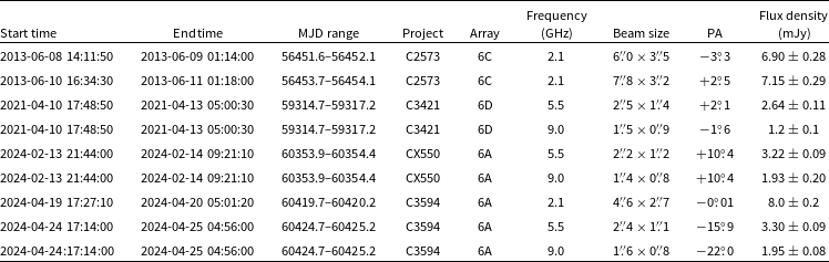
Table 1. Summary of the post-2003 ATCA observations of SN 2001ig.
Tentative identification of 2001ig as a Type IIb was already suggested from optical spectra taken from the 6.5-m Baade Magellan Telescope at Las Campanas Observatory on 2001 December 11–13 (Phillips et al. Reference Phillips, Suntzeff, Krisciunas, Carlberg, Gladders, Barrientos, Matheson and Jha2001). The weakening of the H lines and the general similarity with the template Type Ib SN 1993J (but with faster ejecta velocity) was confirmed with spectra taken from the 3.6-m telescope at the European Southern Observatory over the following month (Clocchiatti & Prieto Reference Clocchiatti and Prieto2001; Clocchiatti Reference Clocchiatti2002). Intensive follow-up optical spectroscopic studies over the first couple of years, with Keck (Filippenko & Chornock Reference Filippenko and Chornock2002; Silverman et al. Reference Silverman, Mazzali, Chornock, Filippenko, Clocchiatti, Phillips, Ganeshalingam and Foley2009), Gemini-South (Ryder et al. Reference Ryder, Murrowood and Stathakis2006) and the Very Large Telescope (Maund et al. Reference Maund, Craig Wheeler, Patat, Wang, Baade and Höflich2007), provided comprehensive coverage of the early hydrogen-rich photospheric phase, then of the disappearance of the hydrogen lines, and finally (after $\approx$
250 days from the explosion) of the nebular phase, dominated by emission lines such as [Mg I]
$\approx$
250 days from the explosion) of the nebular phase, dominated by emission lines such as [Mg I] $\lambda4571$
, [O I]
$\lambda4571$
, [O I] $\lambda\lambda6300,6364$
, and [Ca II]
$\lambda\lambda6300,6364$
, and [Ca II] $\lambda\lambda7291,7324$
(similar to typical Ib SNe). A Gemini/GMOS spectrum at an age of 6 yr (Ryder et al. Reference Ryder2018) showed narrow He II
$\lambda\lambda7291,7324$
(similar to typical Ib SNe). A Gemini/GMOS spectrum at an age of 6 yr (Ryder et al. Reference Ryder2018) showed narrow He II $\lambda4686$
emission, similar to that seen to emerge in SN 2014C 1–2 yr post-explosion (Milisavljevic et al. Reference Milisavljevic2015), and interpreted as continuing interaction with a dense CSM. Broad-band optical photometry, based on Gemini/GMOS images from 2004 September 13 (age
$\lambda4686$
emission, similar to that seen to emerge in SN 2014C 1–2 yr post-explosion (Milisavljevic et al. Reference Milisavljevic2015), and interpreted as continuing interaction with a dense CSM. Broad-band optical photometry, based on Gemini/GMOS images from 2004 September 13 (age $\approx$
1 000 days), shows a yellow counterpart (Fig. 1) consistent with a late-B through late-F supergiant (Ryder et al. Reference Ryder, Murrowood and Stathakis2006). However, Hubble Space Telescope Wide Field Camera 3 images in the near-UV (F275W and F336W filters) from 2016 April 28 (age
$\approx$
1 000 days), shows a yellow counterpart (Fig. 1) consistent with a late-B through late-F supergiant (Ryder et al. Reference Ryder, Murrowood and Stathakis2006). However, Hubble Space Telescope Wide Field Camera 3 images in the near-UV (F275W and F336W filters) from 2016 April 28 (age $\approx$
14.4 yr) showed a fainter, bluer point-like source (Ryder et al. Reference Ryder2018), consistent with a B2 type (
$\approx$
14.4 yr) showed a fainter, bluer point-like source (Ryder et al. Reference Ryder2018), consistent with a B2 type ( $19\,000\,{\mathrm K} \lesssim T_\textrm{eff} \lesssim 22\,000\,{\mathrm K}$
) main sequence star. The discrepancy is possibly due to residual emission from the shocked gas in the earlier observations, while the later observations are consistent with a
$19\,000\,{\mathrm K} \lesssim T_\textrm{eff} \lesssim 22\,000\,{\mathrm K}$
) main sequence star. The discrepancy is possibly due to residual emission from the shocked gas in the earlier observations, while the later observations are consistent with a $\approx$
9 M
$\approx$
9 M $_\odot$
companion star. The likely presence of a surviving companion star supports the scenario that hydrogen stripping in the progenitor of SN 2001ig was caused by binary interaction.
$_\odot$
companion star. The likely presence of a surviving companion star supports the scenario that hydrogen stripping in the progenitor of SN 2001ig was caused by binary interaction.
In the radio bands, high cadence observations were taken over the first $\sim$
3 yr with the ATCA at 1.4, 2.4, 4.8 and 8.6 GHz, with a few, sparser datapoints at 18.8 GHz (Ryder et al. Reference Ryder, Sadler, Subrahmanyan, Weiler, Panagia and Stockdale2004). In addition, the SN was observed a few times with the Very Large Array (VLA) at 1.4, 4.9, 8.5, 15 and 22.5 GHz (Ryder et al. Reference Ryder, Sadler, Subrahmanyan, Weiler, Panagia and Stockdale2004). The data showed (Ryder et al. Reference Ryder, Sadler, Subrahmanyan, Weiler, Panagia and Stockdale2004) a general early trend consistent with the model of Weiler et al. (Reference Weiler, Panagia, Montes and Sramek2002) and Sramek & Weiler (Reference Sramek, Weiler and Weiler2003), with an initial rise (optically thick phase) followed by an asymptotic power-law decline (optically thin phase), with
$\sim$
3 yr with the ATCA at 1.4, 2.4, 4.8 and 8.6 GHz, with a few, sparser datapoints at 18.8 GHz (Ryder et al. Reference Ryder, Sadler, Subrahmanyan, Weiler, Panagia and Stockdale2004). In addition, the SN was observed a few times with the Very Large Array (VLA) at 1.4, 4.9, 8.5, 15 and 22.5 GHz (Ryder et al. Reference Ryder, Sadler, Subrahmanyan, Weiler, Panagia and Stockdale2004). The data showed (Ryder et al. Reference Ryder, Sadler, Subrahmanyan, Weiler, Panagia and Stockdale2004) a general early trend consistent with the model of Weiler et al. (Reference Weiler, Panagia, Montes and Sramek2002) and Sramek & Weiler (Reference Sramek, Weiler and Weiler2003), with an initial rise (optically thick phase) followed by an asymptotic power-law decline (optically thin phase), with $F_\nu \propto (t-t_0)^{-1.5}$
. In the optically thin phase, the spectral index settles at
$F_\nu \propto (t-t_0)^{-1.5}$
. In the optically thin phase, the spectral index settles at $\alpha \approx -1$
. However, there is an interesting modulation, with a period of
$\alpha \approx -1$
. However, there is an interesting modulation, with a period of $\approx 150$
d, superposed on the standard flux evolution (Ryder et al. Reference Ryder, Sadler, Subrahmanyan, Weiler, Panagia and Stockdale2004). This was interpreted as a density modulation of the CSM encountered by the expanding blast wave. One scenario is a series of shell ejections or increased mass loss at regular time intervals over the last few thousand years of the progenitor’s life. This may be the mechanism responsible for the dense dust shells seen around the WR-OB binary WR 112 (Lau et al. Reference Lau, Hankins, Schödel, Sanchez-Bermudez, Moffat and Ressler2017) and the recurrent (optical) re-brightenings over the first year of Type IIn supernova iPTF13z (Nyholm et al. Reference Nyholm2017). Alternatively, Ryder et al. (Reference Ryder, Sadler, Subrahmanyan, Weiler, Panagia and Stockdale2004) suggested that the density enhancements follow a spiral structure (pinwheel or lawn sprinkler model) typical of dust produced by wind-wind collisions near periastron in eccentric massive binary systems. The dusty pinwheel model was theoretically illustrated via hydrodynamical simulations for example by Schwarz & Pringle (Reference Schwarz and Pringle1996) and Walder & Folini (Reference Walder, Folini, van der Hucht, Herrero and Esteban2003), and successfully applied to several observed WR-OB systems (Tuthill, Monnier, & Danchi Reference Tuthill, Monnier and Danchi1999; Monnier, Tuthill, & Danchi Reference Monnier, Tuthill and Danchi1999; Marchenko et al. Reference Marchenko, Moffat, Vacca, Côté and Doyon2002; Soulain et al. Reference Soulain2018).
$\approx 150$
d, superposed on the standard flux evolution (Ryder et al. Reference Ryder, Sadler, Subrahmanyan, Weiler, Panagia and Stockdale2004). This was interpreted as a density modulation of the CSM encountered by the expanding blast wave. One scenario is a series of shell ejections or increased mass loss at regular time intervals over the last few thousand years of the progenitor’s life. This may be the mechanism responsible for the dense dust shells seen around the WR-OB binary WR 112 (Lau et al. Reference Lau, Hankins, Schödel, Sanchez-Bermudez, Moffat and Ressler2017) and the recurrent (optical) re-brightenings over the first year of Type IIn supernova iPTF13z (Nyholm et al. Reference Nyholm2017). Alternatively, Ryder et al. (Reference Ryder, Sadler, Subrahmanyan, Weiler, Panagia and Stockdale2004) suggested that the density enhancements follow a spiral structure (pinwheel or lawn sprinkler model) typical of dust produced by wind-wind collisions near periastron in eccentric massive binary systems. The dusty pinwheel model was theoretically illustrated via hydrodynamical simulations for example by Schwarz & Pringle (Reference Schwarz and Pringle1996) and Walder & Folini (Reference Walder, Folini, van der Hucht, Herrero and Esteban2003), and successfully applied to several observed WR-OB systems (Tuthill, Monnier, & Danchi Reference Tuthill, Monnier and Danchi1999; Monnier, Tuthill, & Danchi Reference Monnier, Tuthill and Danchi1999; Marchenko et al. Reference Marchenko, Moffat, Vacca, Côté and Doyon2002; Soulain et al. Reference Soulain2018).
3. Results of the new radio observations
To investigate the behaviour of SN 2001ig at ages $\gt10$
yr, we used several sets of ATCA observations in the 6-km array configurationFootnote
b
(Table 1); some of the observations were already in the public archives, while others were specifically obtained for this project. These new data were taken between 2013 June and 2024 April, with 2.1 GHz data being taken throughout that entire span, and 5.5 and 9 GHz data being taken from 2021 April until 2024 April, where the 5.5 and 9 GHz data are recorded simultaneously. All new datasets were taken with a bandwidth of 2 GHz around each central frequency (with the Compact Array Broadband Backend; Wilson et al. Reference Wilson2011), compared with the 128 MHz bandwidth of the 2001–2003 data. Details and results from the new ATCA observations are shown in Table 1.
$\gt10$
yr, we used several sets of ATCA observations in the 6-km array configurationFootnote
b
(Table 1); some of the observations were already in the public archives, while others were specifically obtained for this project. These new data were taken between 2013 June and 2024 April, with 2.1 GHz data being taken throughout that entire span, and 5.5 and 9 GHz data being taken from 2021 April until 2024 April, where the 5.5 and 9 GHz data are recorded simultaneously. All new datasets were taken with a bandwidth of 2 GHz around each central frequency (with the Compact Array Broadband Backend; Wilson et al. Reference Wilson2011), compared with the 128 MHz bandwidth of the 2001–2003 data. Details and results from the new ATCA observations are shown in Table 1.
Flux density calibration was done with the primary ATCA calibrator PKS B1934 $-$
638, and phase calibration with the nearby source PKS B2310
$-$
638, and phase calibration with the nearby source PKS B2310 $-$
417. We processed data following standard proceduresFootnote
c
within the Common Astronomy Software Application (casa, version 5.1.2; CASA Team et al. Reference Team2022). Imaging used the casa task clean, using a Briggs robust parameter of 0 (Briggs Reference Briggs1995), which balances sensitivity and resolution. With this choice, we obtained the synthesised beam shapes listed in Table 1.
$-$
417. We processed data following standard proceduresFootnote
c
within the Common Astronomy Software Application (casa, version 5.1.2; CASA Team et al. Reference Team2022). Imaging used the casa task clean, using a Briggs robust parameter of 0 (Briggs Reference Briggs1995), which balances sensitivity and resolution. With this choice, we obtained the synthesised beam shapes listed in Table 1.
To measure the flux density of SN 2001ig, we fit for a point source in the image plane. To do this, we used the casa task imfit to fit a 2D Gaussian with a full-width-at-half-maximum fixed to the parameters of the synthesised beam. All flux density errors include a systematic uncertainty on the absolute flux density of 2% (e.g. Massardi et al. Reference Massardi, Bonaldi, Bonavera, López-Caniego, de Zotti and Ekers2011; McConnell et al. Reference McConnell, Sadler, Murphy and Ekers2012), which was added in quadrature with the measured noise in a source-free region close to the source position.
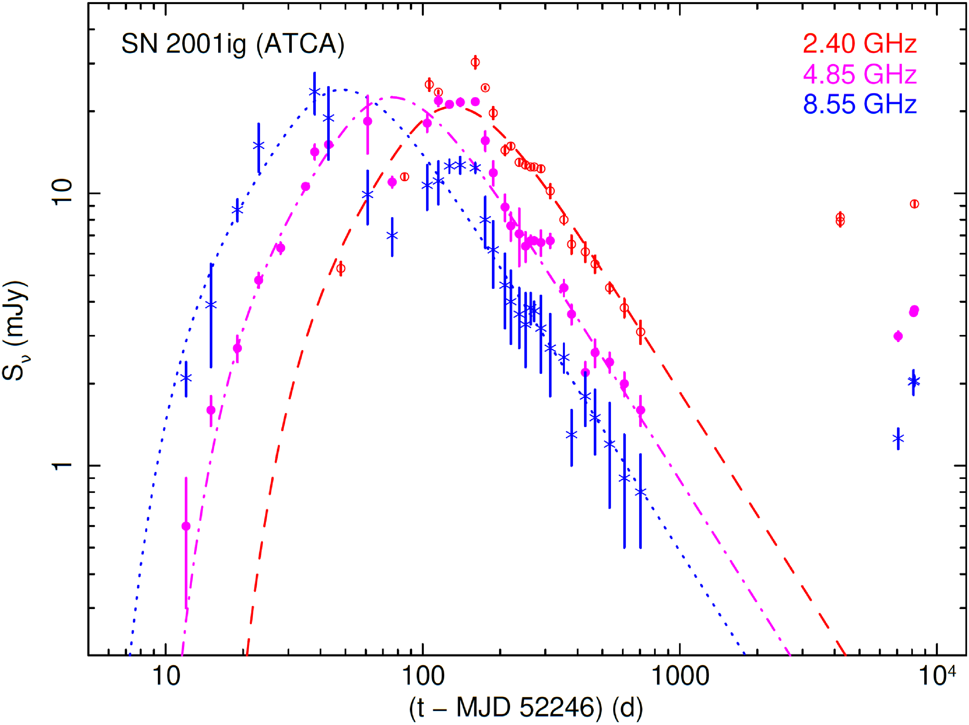
Figure 2. Flux density of SN 2001ig at 2.4, 4.85 and 8.55 GHz, based on ATCA observations, compared with the canonical evolution model of Weiler et al. (Reference Weiler, Panagia, Montes and Sramek2002). The ATCA data from 2001–2003 (Ryder et al. Reference Ryder, Sadler, Subrahmanyan, Weiler, Panagia and Stockdale2004) were taken at central frequencies of 2.4 GHz (red datapoints and dashed line model), 4.85 GHz (magenta datapoints and dash-dotted line model) and 8.55 GHz (blue datapoints and dotted line model), with a bandwidth of 128 MHz. The data from 2013, 2021 and 2024 were taken at central frequencies of 2.1, 5.5 and 9 GHz (Table 1) and then rescaled to 2.4, 4.85 and 8.55 GHz with an assumed spectral index $\alpha = -1$
, for the purposes of this plot. The bandwidth of the 2013, 2021 and 2024 measurements is 2 GHz.
$\alpha = -1$
, for the purposes of this plot. The bandwidth of the 2013, 2021 and 2024 measurements is 2 GHz.
We note that ATCA observations taken on 2024 February 13 suffered from significant phase decorrelation due to poor observing conditions (weather). To address this in the 5.5 GHz data, where there were a number of bright sources in the field, we carried out iterations of phase-only self-calibration, down to a solution interval of 60 s (shorter time intervals did not further improve the image). For the 9 GHz data, we were not able to confidently self-calibrate due to the lack of any sufficiently bright sources in the field (all field sources were $\lt$
5 mJy at 9 GHz). Therefore, to estimate the effects of the phase decorrelation, we re-calibrated the data treating every second scan of the phase calibrator as a ‘target’ and every other phase calibrator scan as the ‘phase calibrator’. Doing so reveals the ‘target’ phase calibrator scans were fainter by a factor of 0.52, indicating strong phase decorrelation. We then correct for this by applying that correction factor to the initial measurement of SN 2001ig (
$\lt$
5 mJy at 9 GHz). Therefore, to estimate the effects of the phase decorrelation, we re-calibrated the data treating every second scan of the phase calibrator as a ‘target’ and every other phase calibrator scan as the ‘phase calibrator’. Doing so reveals the ‘target’ phase calibrator scans were fainter by a factor of 0.52, indicating strong phase decorrelation. We then correct for this by applying that correction factor to the initial measurement of SN 2001ig ( $1.0 \pm 0.1$
mJy).
$1.0 \pm 0.1$
mJy).
We also detected SN 2001ig in a number of Australian SKA Pathfinder (ASKAP; Hotan et al. Reference Hotan2021) observations. These observations were conducted as part of the Rapid ASKAP Continuum Survey (RACS; Hale et al. Reference Hale2021) and Variables and Slow Transients (VAST; Murphy et al. Reference Murphy2021) projects and obtained from the CSIRO ASKAP Science Data ArchiveFootnote
d
(CASDA). Both surveys use the ASKAPSoft pipeline (Cornwell, Voronkov, & Humphreys Reference Cornwell, Voronkov, Humphreys, Bones, Fiddy and Millane2012) for data reduction and the Selavy algorithm (Whiting Reference Whiting2012) to produce fitted source catalogues. RACS and VAST observations, respectively, have $\sim$
15 min and
$\sim$
15 min and $\sim$
12 min integrations, both with a bandwidth of 288 MHz. All epochs of VAST are observed at a central frequency of
$\sim$
12 min integrations, both with a bandwidth of 288 MHz. All epochs of VAST are observed at a central frequency of $887.5$
MHz. RACS includes epochs observed at central frequencies of
$887.5$
MHz. RACS includes epochs observed at central frequencies of $887.5, 943.5,$
and
$887.5, 943.5,$
and $ 1367.5$
MHz. The ASKAP detections are shown in Fig. 3. Flux density errors are calculated as the quadrature sum of the fitted error, RMS, and a 6% flux scale uncertainty.
$ 1367.5$
MHz. The ASKAP detections are shown in Fig. 3. Flux density errors are calculated as the quadrature sum of the fitted error, RMS, and a 6% flux scale uncertainty.
The main results of the late-time radio observations can be summarised as follows:
-
(i) there is strong re-brightening compared with the extrapolated power-law decline of 2001–2002. Today’s radio flux density is two orders of magnitude higher than we expect assuming a simple power-law model. Low-frequency (2.1 GHz) measurements show (Fig. 2) that the re-brightening must have started already before 2013 (age of $\approx$
4 000 d) and more likely, as early as at an age of
$\approx$
1 000 d. At the assumed distance of 10.8 Mpc, the luminosity density at 5.5 GHz was
$\approx$
4.6
$\times 10^{26}$
erg s
$^{-1}$
Hz
$^{-1}$
in 2004 April.
$\approx$
4 000 d) and more likely, as early as at an age of
$\approx$
1 000 d. At the assumed distance of 10.8 Mpc, the luminosity density at 5.5 GHz was
$\approx$
4.6
$\times 10^{26}$
erg s
$^{-1}$
Hz
$^{-1}$
in 2004 April. -
(ii) the re-brightening is still ongoing. There is a slight but significant increase over the past
$\approx$
2 000 d, seen both from ATCA (Fig. 2 and Table 1) and from ASKAP (Fig. 3). -
(iii) the spectral index of the optically thin synchrotron spectrum has remained settled around the canonical value
$\alpha \approx -1$
, a value it had already attained after
$\approx$
1 yr (Ryder et al. Reference Ryder, Sadler, Subrahmanyan, Weiler, Panagia and Stockdale2004). Specifically, the ATCA and ASKAP observations from 2024 April suggest a spectral index
$\alpha \approx -0.93 \pm 0.05$
between 0.89 GHz and 9.0 GHz,
$\alpha \approx -0.97 \pm 0.05$
between 2.1 GHz and 9.0 GHz, and
$\alpha \approx -1.07 \pm 0.05$
between 5.5 GHz and 9.0 GHz. Thus, the re-brightening did not correspond to a change in the spectral slope.


Figure 3. ASKAP detections of SN 2001ig at late times, starting around $\approx 6\,300$
days. The points are coloured by their central observing frequency, with the majority of the observations coming from the
$\approx 6\,300$
days. The points are coloured by their central observing frequency, with the majority of the observations coming from the $887.5$
MHz VAST survey.
$887.5$
MHz VAST survey.
The first hint of an increased CSM interaction leading to a re-brightening was already noted by Ryder et al. (Reference Ryder2018), from the stack of two Gemini/GMOS spectra taken on 2007 July 18 and November 6 (average age $\approx$
2 100 d). The combined spectrum showed narrow HeII
$\approx$
2 100 d). The combined spectrum showed narrow HeII $\lambda4686$
emission, a feature sometimes seen in re-brightening SNe.
$\lambda4686$
emission, a feature sometimes seen in re-brightening SNe.
4. Modelling
We assume that the radio emission is made of an optically thick and an optically thin component (Chevalier Reference Chevalier1998). In the optically thick limit, the flux density, $S_{\nu}$
, is proportional to the observing frequency
$S_{\nu}$
, is proportional to the observing frequency $\nu$
such that
$\nu$
such that $S_{\nu} \propto \nu^{5/2}$
, while in the optically thin limit,
$S_{\nu} \propto \nu^{5/2}$
, while in the optically thin limit, $S_{\nu} \propto \nu^{-(p-1)/2}$
, where p, the spectral index of the particle energies, is
$S_{\nu} \propto \nu^{-(p-1)/2}$
, where p, the spectral index of the particle energies, is $\gt 2$
(typically,
$\gt 2$
(typically, $p \sim 3$
). The peak flux density at a given time is a function of the shock radius
$p \sim 3$
). The peak flux density at a given time is a function of the shock radius $R_{s}$
and the magnetic field strength B (Chevalier Reference Chevalier1998). From
$R_{s}$
and the magnetic field strength B (Chevalier Reference Chevalier1998). From $R_{ s}(t)$
, we can infer the shock velocity
$R_{ s}(t)$
, we can infer the shock velocity $v_{s}$
, the CSM density
$v_{s}$
, the CSM density $\rho_\textrm{csm}$
and other quantities of interest for the evolution of the system.
$\rho_\textrm{csm}$
and other quantities of interest for the evolution of the system.
We model SN 2001ig in two slightly different ways. First, as an initial approximation, we take the observed peak flux density at a given frequency, and assume a value of $p \equiv 3$
and a constant shock velocity to derive
$p \equiv 3$
and a constant shock velocity to derive $\rho_\textrm{ csm}$
. The main purpose of this model is to estimate
$\rho_\textrm{ csm}$
. The main purpose of this model is to estimate $\dot{M}/v_{w}$
of the progenitor star. Then, we use a Markov Chain Monte Carlo (MCMC) model to fit
$\dot{M}/v_{w}$
of the progenitor star. Then, we use a Markov Chain Monte Carlo (MCMC) model to fit $\rho_\textrm{csm}$
at each epoch in order to produce the observed flux density. The main purpose of this model is to estimate the density enhancement encountered by the shock wave at late times.
$\rho_\textrm{csm}$
at each epoch in order to produce the observed flux density. The main purpose of this model is to estimate the density enhancement encountered by the shock wave at late times.
4.1 Determining the mass loss rate of the progenitor
We assume energy equipartition between the magnetic field and the relativistic electrons ( $\alpha = 1$
in the formalism of Chevalier Reference Chevalier1998), with a 10% fraction of post-shock energy going into each component:
$\alpha = 1$
in the formalism of Chevalier Reference Chevalier1998), with a 10% fraction of post-shock energy going into each component: $\epsilon_B = \epsilon_e = 0.1$
. We also assume
$\epsilon_B = \epsilon_e = 0.1$
. We also assume $p \equiv 3$
, corresponding to an optically thin synchrotron spectral index
$p \equiv 3$
, corresponding to an optically thin synchrotron spectral index $\alpha = -1$
, and an emission filling factor (fraction of a spherical volume with outer radius
$\alpha = -1$
, and an emission filling factor (fraction of a spherical volume with outer radius $R_{s}$
)
$R_{s}$
) $f = 0.5$
. Then, the outer shock radius and the magnetic field are obtained from Eqs. (13–14) of Chevalier (Reference Chevalier1998), as a function of the peak flux density
$f = 0.5$
. Then, the outer shock radius and the magnetic field are obtained from Eqs. (13–14) of Chevalier (Reference Chevalier1998), as a function of the peak flux density $S_{\nu,{p}}$
, namely
$S_{\nu,{p}}$
, namely
 \begin{align}R_{s,p} & = 8.8 \times 10^{15} \left(\frac{\epsilon_B}{\epsilon_e}\right)^{1/19}\left(\frac{f}{0.5}\right)^{-1/19} \left(\frac{S_{\nu,{p}}}{{\mathrm {Jy}}}\right)^{9/19}\nonumber \\& \left(\frac{d}{{\mathrm {Mpc}}}\right)^{18/19}\left(\frac{\nu}{5{\mathrm {\,GHz}}}\right)^{-1}\ {\mathrm {{cm}}}\end{align}
 \begin{align}B_{p} & = 0.58 \left(\frac{\epsilon_B}{\epsilon_e}\right)^{4/19}\,\left(\frac{f}{0.5}\right)^{-4/19}\, \left(\frac{S_{\nu,{p}}}{{\mathrm {Jy}}}\right)^{-2/19} \nonumber\\&\left(\frac{d}{{\mathrm {Mpc}}}\right)^{-4/19}\,\left(\frac{\nu}{5{\mathrm {\,GHz}}}\right)^{-1}\ {\mathrm G}\end{align}
For $S_{\nu,{p}}$
,we take the brightest flux density measurement available at any frequency:
$S_{\nu,{p}}$
,we take the brightest flux density measurement available at any frequency: $S_{18.8} \approx 43$
mJy beam
$S_{18.8} \approx 43$
mJy beam $^{-1}$
, from the ATCA at 18.8 GHz at an age
$^{-1}$
, from the ATCA at 18.8 GHz at an age $t-t_0 \approx 28$
d. Thus, the radius of the shocked bubble at that time is
$t-t_0 \approx 28$
d. Thus, the radius of the shocked bubble at that time is $R_{s,p} \approx 5.0 \times 10^{15}$
cm, with a field
$R_{s,p} \approx 5.0 \times 10^{15}$
cm, with a field $B_{p}\approx 1.8$
G. The shock velocity is then simply
$B_{p}\approx 1.8$
G. The shock velocity is then simply $v_{s} = R_{s,p}/(t-t_0) \approx 20\,000$
km s
$v_{s} = R_{s,p}/(t-t_0) \approx 20\,000$
km s $^{-1}$
. To derive the mass loss rate from the progenitor, we use the standard assumption (adopted for example in Rose et al. Reference Rose2024) that the magnetic energy density
$^{-1}$
. To derive the mass loss rate from the progenitor, we use the standard assumption (adopted for example in Rose et al. Reference Rose2024) that the magnetic energy density $B^2/8\pi$
is a fraction
$B^2/8\pi$
is a fraction $\epsilon_B$
of the post shock energy density:
$\epsilon_B$
of the post shock energy density: $B^2/8\pi \approx (9/8)\,\epsilon_B \rho_\textrm{csm}v_{s}^2$
. From Eq. (19) of Chevalier (Reference Chevalier1998), for a constant mass-loss rate in a steady progenitor wind and constant shock velocity, we have:
$B^2/8\pi \approx (9/8)\,\epsilon_B \rho_\textrm{csm}v_{s}^2$
. From Eq. (19) of Chevalier (Reference Chevalier1998), for a constant mass-loss rate in a steady progenitor wind and constant shock velocity, we have:
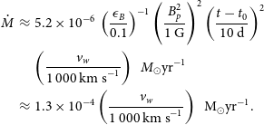 \begin{eqnarray}\dot{M} & \approx & 5.2 \times 10^{-6}\, \left( \frac{\epsilon_B}{0.1}\right)^{-1} \left( \frac{B_{p}^2}{1\ {\mathrm G}} \right)^{2}\left( \frac{t-t_0}{10\ {\mathrm d}}\right)^{2}\nonumber \\&&\left( \frac{v_{w}}{1\,000\ {\mathrm {km~s}}^{-1}}\right)\ \ M_\odot {\rm yr}^{-1}\nonumber \\&\approx& 1.3 \times 10^{-4}\left( \frac{v_{w}}{1\,000\ {\mathrm {km~s}}^{-1}}\right)\ \ {\rm M}_\odot {\rm yr}^{-1}.\end{eqnarray}
At the peak flux density, the CSM density is
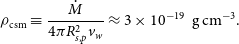 \begin{equation}\rho_\textrm{csm} \equiv \frac{\dot{M}}{4\pi R^2_{s,p}v_{w}} \approx 3 \times 10^{-19}\ \ {\mathrm {g~cm}}^{-3}.\end{equation}
Comparing these values with the physical quantities derived in the ASKAP survey of Rose et al. (Reference Rose2024), we note that the Type Ic SN 2016coi (Grupe et al. Reference Grupe, Brown, Dong, Shappee, Holoien, Stanek, Prieto and Margutti2016; Terreran et al. Reference Terreran2019) appears the most similar to 2001ig at early times.
4.2 Determining the late-time density enhancement
To model the evolution of the synchrotron emission from early to late times, we adopt the thin shell approximation (Cox Reference Cox1972; Castor, McCray, & Weaver Reference Castor, McCray and Weaver1975; Weaver et al. Reference Weaver, McCray, Castor, Shapiro and Moore1977), and solve, via numerical integration, a simultaneous system of equations for the shock radius and velocity at each epoch, the magnetic field, and the peak flux of the synchrotron radiation that results from shock interactions. Specifically, the thin shell differential equation is
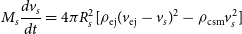 \begin{equation} M_{s} \frac{dv_{s}}{dt} = 4\pi R_{s}^2[\rho_{\textrm{ej}}(v_{\textrm{ej}} - v_{s})^2 - \rho_{\textrm{csm}}v_{s}^2]\end{equation}
(Chevalier & Fransson Reference Chevalier, Fransson, Alsabti and Murdin2017), where $M_{s}$
is the mass of the thin shell comprising shocked ejecta and shocked CSM at the shock radius
$M_{s}$
is the mass of the thin shell comprising shocked ejecta and shocked CSM at the shock radius $R_{s}$
, propagating at the shock velocity
$R_{s}$
, propagating at the shock velocity $v_{s} = dR_{s}/dt$
;
$v_{s} = dR_{s}/dt$
; $v_{\textrm{ej}}$
is the ejecta velocity at the reverse shock;
$v_{\textrm{ej}}$
is the ejecta velocity at the reverse shock; $\rho_{\textrm{ej}}$
and
$\rho_{\textrm{ej}}$
and $\rho_{\textrm{csm}}$
are the density profiles of the shocked ejecta and CSM, respectively.
$\rho_{\textrm{csm}}$
are the density profiles of the shocked ejecta and CSM, respectively. $M_{s}$
is computed from the numerical integration of the density profiles. For the CSM density, we assume again that the post-shock energy density is proportional to the magnetic energy density (
$M_{s}$
is computed from the numerical integration of the density profiles. For the CSM density, we assume again that the post-shock energy density is proportional to the magnetic energy density ( $\rho_\textrm{csm}v_{s}^2 \propto B^2/\epsilon_B$
as in Section 4.2). For the ejecta density profile we adopt
$\rho_\textrm{csm}v_{s}^2 \propto B^2/\epsilon_B$
as in Section 4.2). For the ejecta density profile we adopt
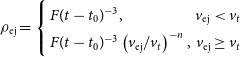 \begin{equation}\rho_{\textrm{ej}} =\left\{ \begin{array}{lr} F(t-t_0)^{-3}, & v_{\textrm{ej}} \lt v_t\\ F(t-t_0)^{-3}\left(v_{\textrm{ej}}/v_t\right)^{-n}, & v_{\textrm{ej}} \geq v_t \end{array}\right.\end{equation}
where
 \begin{equation} F = \frac{1}{4\pi n} \frac{[3(n-3)M_{\textrm{ej}}]^{5/2}}{[10(n-2)E]^{3/2}},\end{equation}
 \begin{equation} v_t = \biggl[\frac{10(n-5)E}{3(n-3)M_{\textrm{ej}}}\biggl]^{1/2},\end{equation}
and $M_\textrm{ej}$
and E are the total explosion mass and energy. Given the uncertainty on the total ejecta mass, we will solve for the CSM profile for a low end estimate of
$M_\textrm{ej}$
and E are the total explosion mass and energy. Given the uncertainty on the total ejecta mass, we will solve for the CSM profile for a low end estimate of $M_{ej} = 1\,{\rm M}_\odot$
(approximately the ejecta mass estimated by Silverman et al. Reference Silverman, Mazzali, Chornock, Filippenko, Clocchiatti, Phillips, Ganeshalingam and Foley2009) and a high end estimate of
$M_{ej} = 1\,{\rm M}_\odot$
(approximately the ejecta mass estimated by Silverman et al. Reference Silverman, Mazzali, Chornock, Filippenko, Clocchiatti, Phillips, Ganeshalingam and Foley2009) and a high end estimate of $M_{ej} = 4\,{\rm M}_\odot$
; stripped-envelope SN models by Aguilera-Dena et al. (Reference Aguilera-Dena, Müller, Antoniadis, Langer, Dessart, Vigna-Gómez and Yoon2023) suggest that the mass range between 1 and 4 M
$M_{ej} = 4\,{\rm M}_\odot$
; stripped-envelope SN models by Aguilera-Dena et al. (Reference Aguilera-Dena, Müller, Antoniadis, Langer, Dessart, Vigna-Gómez and Yoon2023) suggest that the mass range between 1 and 4 M $_\odot$
covers about 80% of events. For the 1 M
$_\odot$
covers about 80% of events. For the 1 M $_\odot$
model, we assume a fixed explosion energy of
$_\odot$
model, we assume a fixed explosion energy of $E = 10^{51}$
erg, corresponding to an initial ejecta velocity of
$E = 10^{51}$
erg, corresponding to an initial ejecta velocity of $v_i \approx 10\,000$
km/s. For the 4 M
$v_i \approx 10\,000$
km/s. For the 4 M $_\odot$
model, instead, we find that the using the same explosion energy results in an initial ejecta velocity,
$_\odot$
model, instead, we find that the using the same explosion energy results in an initial ejecta velocity, $v_i \approx 5\,000$
km/s that is too slow to reproduce the observed early time emission with any density profile. In order to obtain an acceptable flux density fit for this high value of
$v_i \approx 5\,000$
km/s that is too slow to reproduce the observed early time emission with any density profile. In order to obtain an acceptable flux density fit for this high value of $M_{\textrm{ej}}$
, we allow the initial ejecta velocity to be a free parameter,
$M_{\textrm{ej}}$
, we allow the initial ejecta velocity to be a free parameter, $v_{{i}}$
. For this higher mass scenario we find that an initial ejecta velocity of
$v_{{i}}$
. For this higher mass scenario we find that an initial ejecta velocity of $v_i = 13\,888$
km/s is needed to replicate the early time emission. Finally, we adopt an ejecta density index
$v_i = 13\,888$
km/s is needed to replicate the early time emission. Finally, we adopt an ejecta density index $n = 10$
, suitable for massive stars with radiative envelopes and convective cores (Chevalier Reference Chevalier1982a; Matzner & McKee Reference Matzner and McKee1999; Chevalier & Fransson Reference Chevalier, Fransson, Alsabti and Murdin2017), including Wolf-Rayet stars (Kippenhahn & Weigert Reference Kippenhahn and Weigert1990).
$n = 10$
, suitable for massive stars with radiative envelopes and convective cores (Chevalier Reference Chevalier1982a; Matzner & McKee Reference Matzner and McKee1999; Chevalier & Fransson Reference Chevalier, Fransson, Alsabti and Murdin2017), including Wolf-Rayet stars (Kippenhahn & Weigert Reference Kippenhahn and Weigert1990).
In addition to Eq. (5) for the shock dynamics, and the equations for ejecta and CSM density, we simultaneously solve Eqs. (11–12) from Chevalier (Reference Chevalier1998) to infer the peak flux density $S_{\nu,{p}}$
and peak frequency
$S_{\nu,{p}}$
and peak frequency $\nu_{p}$
from the calculated radius and magnetic field strength at each epoch. As we did in Section 4.1, we assume that the fractions of post-shock energy transferred to the magnetic field and the relativistic electrons are
$\nu_{p}$
from the calculated radius and magnetic field strength at each epoch. As we did in Section 4.1, we assume that the fractions of post-shock energy transferred to the magnetic field and the relativistic electrons are $\epsilon_B = 0.1$
and
$\epsilon_B = 0.1$
and $\epsilon_e = 0.1$
, respectively, and that these fractions do not evolve with time; we assume again a standard filling factor,
$\epsilon_e = 0.1$
, respectively, and that these fractions do not evolve with time; we assume again a standard filling factor, $f = 0.5$
. We then model the radio spectrum as a broken power law, with an optically thick slope of 5/2 and an optically thin slope of
$f = 0.5$
. We then model the radio spectrum as a broken power law, with an optically thick slope of 5/2 and an optically thin slope of $(1-p)/2$
:
$(1-p)/2$
:
 \begin{equation} S_\nu = 2 S_{\nu,{p}} \left[ \left(\frac{\nu}{\nu_{{p}}}\right)^{-(1-p)/2} + \left(\frac{\nu}{\nu_{{p}}}\right)^{-5/2}\right]^{-1}.\end{equation}
Unlike what we did in Section 4.1, here we do not assume a spectral index $p=3$
for the electron energies; instead, we fit our broken power-law spectrum across all epochs with an MCMC fit (with the python package emcee
Footnote
e
), and find that the best fitting value is constrained to be
$p=3$
for the electron energies; instead, we fit our broken power-law spectrum across all epochs with an MCMC fit (with the python package emcee
Footnote
e
), and find that the best fitting value is constrained to be $p = 2.83 \pm 0.02$
.
$p = 2.83 \pm 0.02$
.
We assume that at early times, $(t-t_0) \lt 700$
d, the SN shock is interacting with a CSM density profile that scales as
$(t-t_0) \lt 700$
d, the SN shock is interacting with a CSM density profile that scales as $\rho_{\textrm{csm}}\propto R^{-\alpha}$
. Using an MCMC to model the shock dynamics and resulting radiation for just the early time data, we infer
$\rho_{\textrm{csm}}\propto R^{-\alpha}$
. Using an MCMC to model the shock dynamics and resulting radiation for just the early time data, we infer $\alpha = 1.96\pm 0.01$
. We thus assume a standard wind density profile (
$\alpha = 1.96\pm 0.01$
. We thus assume a standard wind density profile ( $\rho_{\textrm{csm}} \propto R^{-2}$
) at smaller radii. Our main objective here is to explain the observed radio re-brightening at late times (Fig. 2). We want to test whether a deviation from the CSM wind-density profile at large radii can explain the re-brightening, and if so, what amount of density enhancement may be needed. To this aim, we introduce a break radius
$\rho_{\textrm{csm}} \propto R^{-2}$
) at smaller radii. Our main objective here is to explain the observed radio re-brightening at late times (Fig. 2). We want to test whether a deviation from the CSM wind-density profile at large radii can explain the re-brightening, and if so, what amount of density enhancement may be needed. To this aim, we introduce a break radius $R_{\rm{brk}}$
, where the shock encounters an over-density compared to the extrapolation of the wind-density profile, and starts to interact with a CSM characterised by shallower density index,
$R_{\rm{brk}}$
, where the shock encounters an over-density compared to the extrapolation of the wind-density profile, and starts to interact with a CSM characterised by shallower density index, $\alpha_{\rm{over}}$
. For a detailed description of the model, in the more general case of a three-zone CSM, see Ibik et al. (Reference Ibik2024).
$\alpha_{\rm{over}}$
. For a detailed description of the model, in the more general case of a three-zone CSM, see Ibik et al. (Reference Ibik2024).
We use another MCMC fit to solve for the CSM profile that would produce the observed emission. The fit parameters are: $R_{\textrm{brk}}$
,
$R_{\textrm{brk}}$
, $\rho_{\textrm{0,wind}}$
,
$\rho_{\textrm{0,wind}}$
, $\rho_{\textrm{0,over}}$
, and
$\rho_{\textrm{0,over}}$
, and $\alpha_{\textrm{over}}$
.
$\alpha_{\textrm{over}}$
. $R_{\textrm{brk}}$
represents the radius at which the shock encounters an overdensity;
$R_{\textrm{brk}}$
represents the radius at which the shock encounters an overdensity; $\rho_{\textrm{0,wind}}$
and
$\rho_{\textrm{0,wind}}$
and $\rho_{\textrm{0,over}}$
are the CSM densities immediately before and after
$\rho_{\textrm{0,over}}$
are the CSM densities immediately before and after $R_{\textrm{brk}}$
. We assume that the CSM follows a wind density profile (
$R_{\textrm{brk}}$
. We assume that the CSM follows a wind density profile ( $\rho_{\textrm{csm}} \propto R^{-2}$
) at
$\rho_{\textrm{csm}} \propto R^{-2}$
) at $R \lt R_{\textrm{brk}}$
and a shallower profile
$R \lt R_{\textrm{brk}}$
and a shallower profile $\rho_{\textrm{csm}} \propto R^{-\alpha_{\textrm{over}}}$
at
$\rho_{\textrm{csm}} \propto R^{-\alpha_{\textrm{over}}}$
at $R \gt R_{\textrm{brk}}$
:
$R \gt R_{\textrm{brk}}$
:
 \begin{equation}\rho_{\textrm{CSM}} =\left\{ \begin{array}{lr} \rho_\textrm{0, wind} \left(R/R_\textrm{brk}\right)^{-2}, & R \lt R_\textrm{brk}\\ \rho_\textrm{0, over} \left(R/R_\textrm{brk}\right)^{-\alpha_\textrm{over}}, & R \gt R_\textrm{brk} \end{array}\right.\end{equation}
For this treatment of the shock dynamics, we expect the shock velocity to decrease steadily over time, as the shock propagates through power law CSM profiles. At the density discontinuity $R_\textrm{brk}$
, the rate of deceleration will change as the shock encounters an overdensity, with a potentially different power law index,
$R_\textrm{brk}$
, the rate of deceleration will change as the shock encounters an overdensity, with a potentially different power law index, $\alpha_\textrm{over}$
. With this evolution, we expect the overall flux density to steadily decline as the shock velocity decreases along the wind density section of the CSM profile. When encountering the overdensity at
$\alpha_\textrm{over}$
. With this evolution, we expect the overall flux density to steadily decline as the shock velocity decreases along the wind density section of the CSM profile. When encountering the overdensity at $R_\textrm{brk}$
, the flux density will increase as the shock accelerates a larger population of electrons to produce synchrotron emission. At very late times (
$R_\textrm{brk}$
, the flux density will increase as the shock accelerates a larger population of electrons to produce synchrotron emission. At very late times ( $(t-t_0) \gtrsim 2 \times 10^{4}$
d and
$(t-t_0) \gtrsim 2 \times 10^{4}$
d and $(t-t_0) \gtrsim 5 \times 10^{4}$
d for the low and high
$(t-t_0) \gtrsim 5 \times 10^{4}$
d for the low and high $M_{\textrm{ej}}$
scenarios, respectively), the flux density will once again begin to decline, as the shock velocity keeps decreasing.
$M_{\textrm{ej}}$
scenarios, respectively), the flux density will once again begin to decline, as the shock velocity keeps decreasing.
The best-fitting CSM density profiles for the low and high $M_{\textrm{ej}}$
scenarios are shown in Fig. 4, and the corresponding time evolutions of the model flux densities are plotted in Fig. 5 and (for the representative 5-GHz case) Fig. 6: lightcurve. Details of the fit results for each parameter are in the Appendix, Figs. A1–A2. Although the density jump at the break radius is somewhat small in both cases, this increase, in combination with the shallower power-law index
$M_{\textrm{ej}}$
scenarios are shown in Fig. 4, and the corresponding time evolutions of the model flux densities are plotted in Fig. 5 and (for the representative 5-GHz case) Fig. 6: lightcurve. Details of the fit results for each parameter are in the Appendix, Figs. A1–A2. Although the density jump at the break radius is somewhat small in both cases, this increase, in combination with the shallower power-law index $\alpha_{\rm{over}}$
, creates an overdensity of about an order of magnitude at the most recent epochs of observation (year 2024) compared to what it would have been in case of a standard wind profile. This, in turn, leads to radio flux densities about two orders of magnitude higher than expected from the extrapolation of the early-time decline. The best fit value for
$\alpha_{\rm{over}}$
, creates an overdensity of about an order of magnitude at the most recent epochs of observation (year 2024) compared to what it would have been in case of a standard wind profile. This, in turn, leads to radio flux densities about two orders of magnitude higher than expected from the extrapolation of the early-time decline. The best fit value for $\alpha_{\rm{over}}$
remains constant across both fits, at
$\alpha_{\rm{over}}$
remains constant across both fits, at $\alpha_{\rm{over}} = 0.75$
. This shallow index, corresponding to a slow evolution of CSM density, is needed to reproduce the slow evolution of synchrotron emission after the re-brightening.
$\alpha_{\rm{over}} = 0.75$
. This shallow index, corresponding to a slow evolution of CSM density, is needed to reproduce the slow evolution of synchrotron emission after the re-brightening.
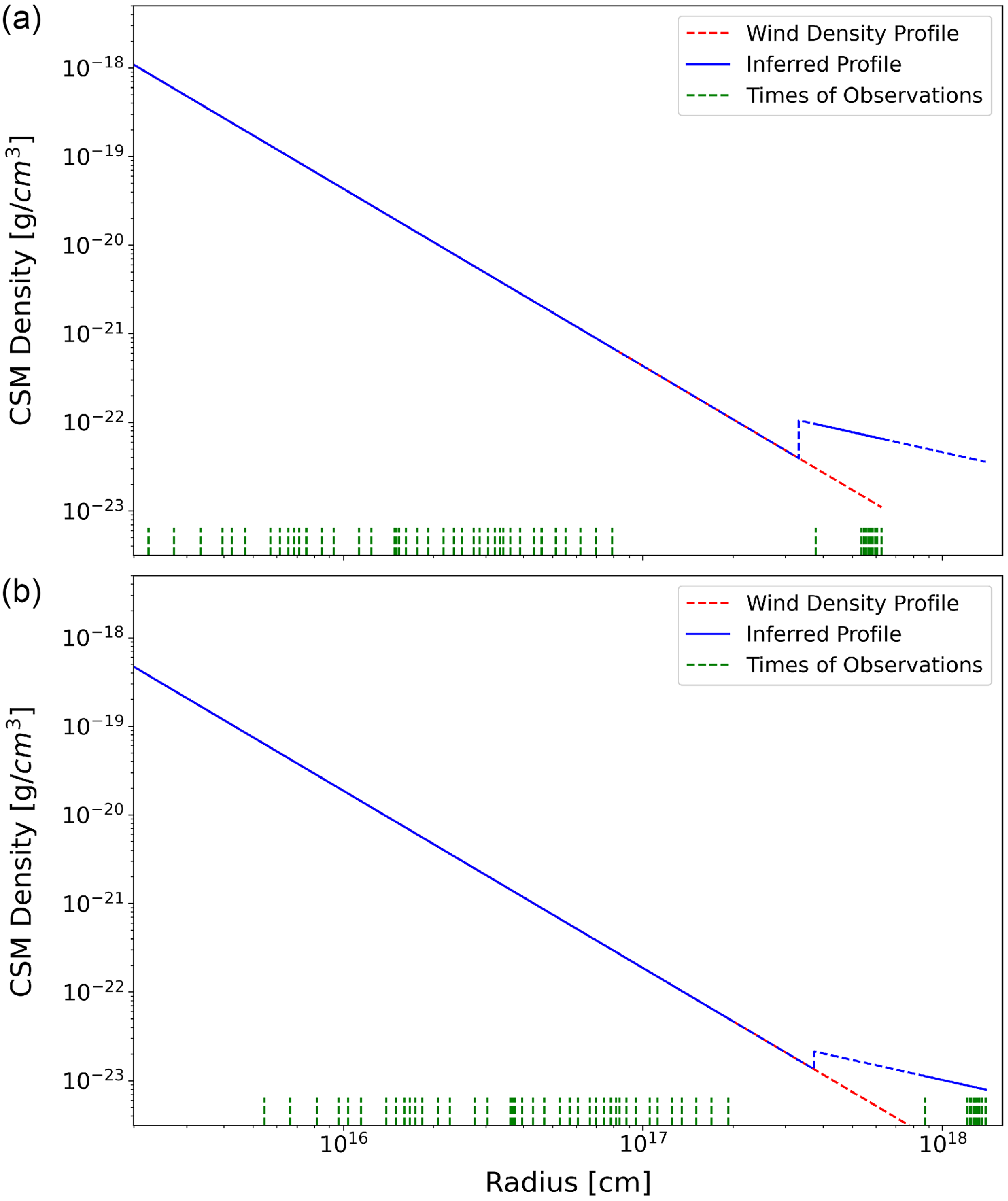
Figure 4. Inferred CSM density profiles as a function of shock radius, for (a) $M_{\rm{ej}} = 1\,{\rm M}_\odot$
, and (b)
$M_{\rm{ej}} = 1\,{\rm M}_\odot$
, and (b) $M_{\rm{ej}} = 4\,{\rm M}_\odot$
. In each panel, the blue line is our model density profile that provides the best fit to the observed radio datapoints at early and late times; the dashed red line is the density profile assuming a uniform stellar wind (
$M_{\rm{ej}} = 4\,{\rm M}_\odot$
. In each panel, the blue line is our model density profile that provides the best fit to the observed radio datapoints at early and late times; the dashed red line is the density profile assuming a uniform stellar wind ( $\rho_{\textrm{csm}} \propto R^{-2}$
). The green markers on the X axis represent the best-fitting shock radius at each of the epochs with radio observations. The gap in the radio coverage between ages of
$\rho_{\textrm{csm}} \propto R^{-2}$
). The green markers on the X axis represent the best-fitting shock radius at each of the epochs with radio observations. The gap in the radio coverage between ages of $\approx$
2–12 yr creates an uncertainty about where the density enhancement occurs (i.e. the parameter
$\approx$
2–12 yr creates an uncertainty about where the density enhancement occurs (i.e. the parameter $R_{\textrm{brk}}$
in our model, Section 4.2). The portions of the CSM density profiles well constrained by the radio observations are plotted as solid blue segments, while the intervals without a strong constraint are dashed.
$R_{\textrm{brk}}$
in our model, Section 4.2). The portions of the CSM density profiles well constrained by the radio observations are plotted as solid blue segments, while the intervals without a strong constraint are dashed.
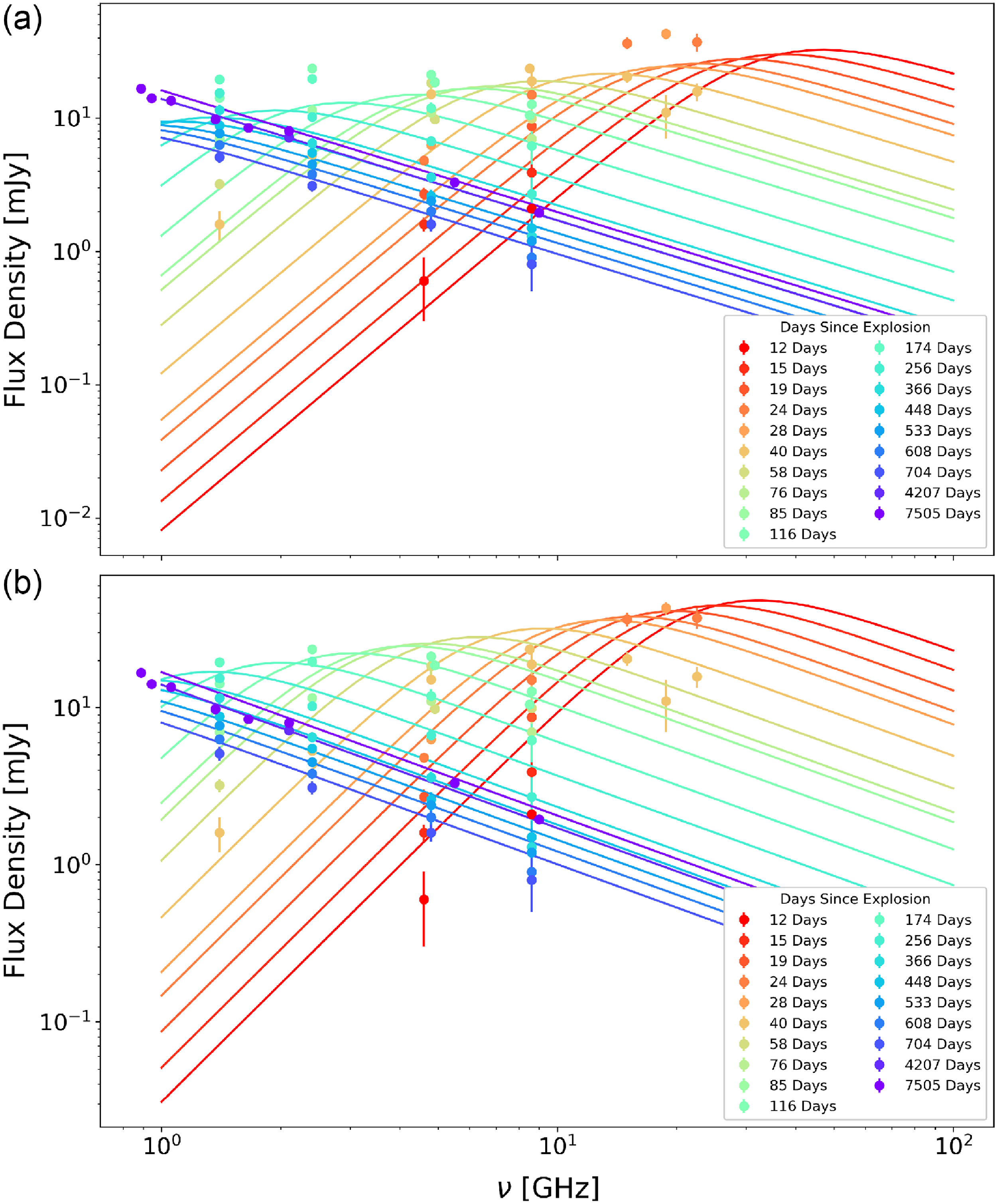
Figure 5. Spectral energy distributions of the best-fitting models for (a) $M_{\rm{ej}} = 1\,{\rm M}_\odot$
, and (b)
$M_{\rm{ej}} = 1\,{\rm M}_\odot$
, and (b) $M_{\rm{ej}} = 4\,{\rm M}_\odot$
, at each time step. Datapoints (solid circles) are the observed radio flux densities, colour-coded by SN age, from red (earliest) to violet (latest). Consecutive observations with
$M_{\rm{ej}} = 4\,{\rm M}_\odot$
, at each time step. Datapoints (solid circles) are the observed radio flux densities, colour-coded by SN age, from red (earliest) to violet (latest). Consecutive observations with $\Delta t/t \lt 0.1$
are combined, and their plotted colour corresponds to the average age. Solid lines are model radio spectra (also colour-coded by age) corresponding to our best-fitting CSM density profile and shock velocity. At earlier times, flux density and peak frequency decrease over time, as expected from a slowly decelerating shock propagating through a uniformly expanding wind. At later times, the flux increases again, which we interpret as a flattening of the CSM density profile.
$\Delta t/t \lt 0.1$
are combined, and their plotted colour corresponds to the average age. Solid lines are model radio spectra (also colour-coded by age) corresponding to our best-fitting CSM density profile and shock velocity. At earlier times, flux density and peak frequency decrease over time, as expected from a slowly decelerating shock propagating through a uniformly expanding wind. At later times, the flux increases again, which we interpret as a flattening of the CSM density profile.

Figure 6. Flux density evolution of the best-fitting spectral model for (a) $M_{\rm{ej}} = 1\,{\rm M}_\odot$
, and (b)
$M_{\rm{ej}} = 1\,{\rm M}_\odot$
, and (b) $M_{\rm{ej}} = 4\,{\rm M}_\odot$
, for the representative 5-GHz case, compared with the observed datapoints (red circles).
$M_{\rm{ej}} = 4\,{\rm M}_\odot$
, for the representative 5-GHz case, compared with the observed datapoints (red circles).
As a caveat, we stress that the lack of data between $\approx$
3–10 yr post-explosion creates uncertainty as to where exactly the overdensity begins. This can clearly be seen from the large gap between the fitted values of the shock radii at each epoch of observations, marked as green segments on the X axis of Fig. 4; the overdensity begins somewhere within that gap. As a result, although our best-fitting parameters represent one solution in good agreement with the observations, there are still strong degeneracies between
$\approx$
3–10 yr post-explosion creates uncertainty as to where exactly the overdensity begins. This can clearly be seen from the large gap between the fitted values of the shock radii at each epoch of observations, marked as green segments on the X axis of Fig. 4; the overdensity begins somewhere within that gap. As a result, although our best-fitting parameters represent one solution in good agreement with the observations, there are still strong degeneracies between $R_{\textrm{brk}}$
and the normalisations of
$R_{\textrm{brk}}$
and the normalisations of $\rho_{\textrm{0,wind}}$
and
$\rho_{\textrm{0,wind}}$
and $\rho_{\textrm{0,over}}$
. A different combination of break radius and overdensity normalisation could produce the same densities at the points where we actually have measurements.
$\rho_{\textrm{0,over}}$
. A different combination of break radius and overdensity normalisation could produce the same densities at the points where we actually have measurements.
The best-fitting density profiles in Fig. 4 reach fairly low densities (number densities $n_e \sim 10$
–100 cm
$n_e \sim 10$
–100 cm $^{-3}$
), especially in the case of high
$^{-3}$
), especially in the case of high $M_{\textrm{ej}}$
. However, this is a direct result of our choice of the microphysical parameter
$M_{\textrm{ej}}$
. However, this is a direct result of our choice of the microphysical parameter $\epsilon_B = 0.1$
. Some models of non-relativistic shock acceleration predict values of
$\epsilon_B = 0.1$
. Some models of non-relativistic shock acceleration predict values of $\epsilon_B$
an order of magnitude lower (Gupta, Caprioli, & Spitkovsky Reference Gupta, Caprioli and Spitkovsky2024). If we were to assume a lower fraction of the total energy transferred to the magnetic field strength, we would in turn infer higher densities, to produce the same observed radio emission. Therefore, our density models can best be interpreted as lower limits on the CSM density profile. While the density normalisation remains uncertain, the inferred trend of a flattening density index at late times is a solid result regardless of the choices of
$\epsilon_B$
an order of magnitude lower (Gupta, Caprioli, & Spitkovsky Reference Gupta, Caprioli and Spitkovsky2024). If we were to assume a lower fraction of the total energy transferred to the magnetic field strength, we would in turn infer higher densities, to produce the same observed radio emission. Therefore, our density models can best be interpreted as lower limits on the CSM density profile. While the density normalisation remains uncertain, the inferred trend of a flattening density index at late times is a solid result regardless of the choices of $M_{\textrm{ej}}$
and
$M_{\textrm{ej}}$
and $\epsilon_B$
.
$\epsilon_B$
.
5. Discussion and conclusion
With new ATCA and ASKAP observations two decades after the event, we report a radio re-brightening of SN 2001ig. The remnant is now two orders of magnitude brighter than expected from the extrapolation of its initial power-law decline, which was well monitored during the first 2 yr. The increase in radio brightness is still ongoing; the most recent measurement of the luminosity density at 5.5 GHz was $\approx$
4.6
$\approx$
4.6 $\times 10^{26}$
erg s
$\times 10^{26}$
erg s $^{-1}$
Hz
$^{-1}$
Hz $^{-1}$
in 2004 April. Despite the radio flux changes, the spectral index has remained constant at
$^{-1}$
in 2004 April. Despite the radio flux changes, the spectral index has remained constant at $\alpha \approx -1.0$
, typical of the optically thin emission expected in radio SNe. This finding suggests that the re-brightening is caused by the shock wave passing through a denser CSM region; in fact, the ambient density encountered by the shock may still be declining with radius, but slower than the canonical
$\alpha \approx -1.0$
, typical of the optically thin emission expected in radio SNe. This finding suggests that the re-brightening is caused by the shock wave passing through a denser CSM region; in fact, the ambient density encountered by the shock may still be declining with radius, but slower than the canonical $R^{-2}$
wind profile. Other scenarios for the re-brightening are more contrived or ruled out. For example, in the young pulsar wind nebula scenario, a flattening of the radio spectral index would have been expected. The off-axis jet scenario is also disfavoured by our data owing to the shape of the radio light-curve, with a peak at early times, a decline, and a re-brightening two decades later (see the discussion of this scenario and its shortcomings in Stroh et al. Reference Stroh2021). At the current age, the CSM over-density required to explain the flux increase is about an order of magnitude above the extrapolated wind density profile. From our modelling of the radio flux density evolution at early and late times, we estimate that the denser layer was encountered when the shock reached a distance of
$R^{-2}$
wind profile. Other scenarios for the re-brightening are more contrived or ruled out. For example, in the young pulsar wind nebula scenario, a flattening of the radio spectral index would have been expected. The off-axis jet scenario is also disfavoured by our data owing to the shape of the radio light-curve, with a peak at early times, a decline, and a re-brightening two decades later (see the discussion of this scenario and its shortcomings in Stroh et al. Reference Stroh2021). At the current age, the CSM over-density required to explain the flux increase is about an order of magnitude above the extrapolated wind density profile. From our modelling of the radio flux density evolution at early and late times, we estimate that the denser layer was encountered when the shock reached a distance of $\approx$
3
$\approx$
3 $\times 10^{17}$
cm
$\times 10^{17}$
cm $\approx 0.1$
pc. The mass-loss rate of the progenitor immediately before the explosion is estimated at
$\approx 0.1$
pc. The mass-loss rate of the progenitor immediately before the explosion is estimated at $\dot{M}/v_{w} \approx 1.3 \times 10^{-7}\,{\rm M}_\odot {{\rm~yr}}^{-1} {\mathrm {km}}^{-1} {\mathrm {s}}$
. We stress that this solution is based on a simple two-zone structure of the CSM, with a density jump between them, justified by the limited number of late-time datapoints available so far. Alternative solutions based on more complex density structures, for example with the presence of a finite-width, high-density wall between the ejecta and the inner part of the CSM (Harris & Nugent Reference Harris and Nugent2020), are left to follow-up work.
$\dot{M}/v_{w} \approx 1.3 \times 10^{-7}\,{\rm M}_\odot {{\rm~yr}}^{-1} {\mathrm {km}}^{-1} {\mathrm {s}}$
. We stress that this solution is based on a simple two-zone structure of the CSM, with a density jump between them, justified by the limited number of late-time datapoints available so far. Alternative solutions based on more complex density structures, for example with the presence of a finite-width, high-density wall between the ejecta and the inner part of the CSM (Harris & Nugent Reference Harris and Nugent2020), are left to follow-up work.
The re-brightening of Type IIb SN 2001ig differs from the behaviour shown by the well-studied Type IIb SN 1993J, whose late-time radio flux dropped sharply below the extrapolated decline model. Such behaviour is consistent with the interpretation of Type IIb SNe as a mixed class, some with extended red/yellow supergiant progenitors (slower winds and late-time radio downturn) and others with compact Wolf-Rayet or stripped progenitors (late-time re-brightening). SN 2001ig joins the small but growing sample of re-brightening SNe, previously identified from the VLA Sky Survey (Stroh et al. Reference Stroh2021) and from the ASKAP Variables and Slow Transients survey (Rose et al. Reference Rose2024). Its proximity to us makes it one of the best such sources for follow-up studies.
Type IIb SN 2003bg ( $d \approx 19.5$
Mpc) is one of the best analogues of 2001ig (Soderberg et al. Reference Soderberg, Chevalier, Kulkarni and Frail2006; Rose et al. Reference Rose2024). Both have shown recurrent flux modulations at early times, and re-brightenings at late times. Both are consistent with a Wolf-Rayet progenitor with mass loss rates
$d \approx 19.5$
Mpc) is one of the best analogues of 2001ig (Soderberg et al. Reference Soderberg, Chevalier, Kulkarni and Frail2006; Rose et al. Reference Rose2024). Both have shown recurrent flux modulations at early times, and re-brightenings at late times. Both are consistent with a Wolf-Rayet progenitor with mass loss rates $\dot{M}\sim 10^{-4}\,{\rm M}_\odot {\rm yr}^{-1}$
. However, the shock velocity in 2003bg is estimated to be
$\dot{M}\sim 10^{-4}\,{\rm M}_\odot {\rm yr}^{-1}$
. However, the shock velocity in 2003bg is estimated to be $\approx$
58 000 km s
$\approx$
58 000 km s $^{-1}$
(Rose et al. Reference Rose2024), significantly higher than the plausible range of shock velocities we inferred for 2001ig (
$^{-1}$
(Rose et al. Reference Rose2024), significantly higher than the plausible range of shock velocities we inferred for 2001ig ( $v_{\mathrm{s}} \sim 10\,000$
–20 000 km s
$v_{\mathrm{s}} \sim 10\,000$
–20 000 km s $^{-1}$
depending on the model assumptions). Moreover, the peak luminosity of 2003bg is an order of magnitude higher, and the CSM density at peak luminosity is an order of magnitude lower (Rose et al. Reference Rose2024). Type Ic SN 2016coi is a close analog of 2001ig in terms of
$^{-1}$
depending on the model assumptions). Moreover, the peak luminosity of 2003bg is an order of magnitude higher, and the CSM density at peak luminosity is an order of magnitude lower (Rose et al. Reference Rose2024). Type Ic SN 2016coi is a close analog of 2001ig in terms of $v_{\mathrm{sh}}$
, early-time
$v_{\mathrm{sh}}$
, early-time $\rho_{\mathrm{csm}}$
, and
$\rho_{\mathrm{csm}}$
, and $\dot{M}/v_{{w}}$
(Rose et al. Reference Rose2024). However, 2016coi is thought to come from a single stellar progenitor rather than a binary (Terreran et al. Reference Terreran2019) and does not show significant late-time radio re-brightening (Rose et al. Reference Rose2024).
$\dot{M}/v_{{w}}$
(Rose et al. Reference Rose2024). However, 2016coi is thought to come from a single stellar progenitor rather than a binary (Terreran et al. Reference Terreran2019) and does not show significant late-time radio re-brightening (Rose et al. Reference Rose2024).
The simplest explanation for late-time re-brightenings is that SN 2001ig exploded in a low-density bubble surrounded by a denser shell with an inner wall at $R \sim v_{s}\, \delta t \approx 0.06\ (v_{s}/2 \times 10^4\ \textrm{ km~s}^{-1})\,(\delta t/1\,000\ \textrm{d})$
pc, where
$R \sim v_{s}\, \delta t \approx 0.06\ (v_{s}/2 \times 10^4\ \textrm{ km~s}^{-1})\,(\delta t/1\,000\ \textrm{d})$
pc, where $\delta t$
is the age at which the shock reached the denser shell. Type Ib/IIn SN 2014C arguably provides the best observational evidence (from radio to hard X-rays) of an interaction of the fast SN shock with the slower, denser shell of
$\delta t$
is the age at which the shock reached the denser shell. Type Ib/IIn SN 2014C arguably provides the best observational evidence (from radio to hard X-rays) of an interaction of the fast SN shock with the slower, denser shell of $\approx$
1 M
$\approx$
1 M $_\odot$
of hydrogen-rich material at
$_\odot$
of hydrogen-rich material at $\approx$
6
$\approx$
6 $\times 10^{16}$
cm
$\times 10^{16}$
cm $\approx$
0.02 pc (Margutti et al. Reference Margutti2017; Brethauer et al. Reference Brethauer, Margutti, Milisavljevic and Bietenholz2020).
$\approx$
0.02 pc (Margutti et al. Reference Margutti2017; Brethauer et al. Reference Brethauer, Margutti, Milisavljevic and Bietenholz2020).
The physical origin of the denser shell is still unclear, and may differ from system to system. A simple explanation is that a shell can be interstellar gas and/or slower wind from an earlier red supergiant phase of the progenitor or of the binary companion, swept-up by the faster Wolf-Rayet wind in the centuries before the explosion. An alternative possibility is that the shell was part of the envelope of the progenitor star, ejected via some kind of internal instability. In the case of SN 2001ig, the progenitor star is not massive enough to be a Luminous Blue Variable or $\eta$
-Carinae-like star, in which shell ejections are well known; however, other forms of instability may exist. For example, Quataert & Shiode (Reference Quataert and Shiode2012) proposed that convection inside C-fusing stars can drive internal gravity waves, which are then converted to acoustic waves. Such waves carry a super-Eddington amount of power; their dissipation in the stellar envelope can unbind up to several
$\eta$
-Carinae-like star, in which shell ejections are well known; however, other forms of instability may exist. For example, Quataert & Shiode (Reference Quataert and Shiode2012) proposed that convection inside C-fusing stars can drive internal gravity waves, which are then converted to acoustic waves. Such waves carry a super-Eddington amount of power; their dissipation in the stellar envelope can unbind up to several $M_\odot$
of H-rich material and trigger massive outflows. Another intriguing scenario (Margutti et al. Reference Margutti2017) is that the presence of a denser shell, and therefore of a late-time re-brightening, is a signature of a binary progenitor system. Specifically, binary interactions may cause runaway mass transfer, followed by a common envelope, then by the ejection of the common envelope at low speeds. The leftover stripped star is the one that explodes as a SN. Finally, the fast ejecta interact with the slow expanding common envelope.
$M_\odot$
of H-rich material and trigger massive outflows. Another intriguing scenario (Margutti et al. Reference Margutti2017) is that the presence of a denser shell, and therefore of a late-time re-brightening, is a signature of a binary progenitor system. Specifically, binary interactions may cause runaway mass transfer, followed by a common envelope, then by the ejection of the common envelope at low speeds. The leftover stripped star is the one that explodes as a SN. Finally, the fast ejecta interact with the slow expanding common envelope.
We plan to continue regular radio monitoring of SN 2001ig over the coming years, aiming to determine the thickness and total mass of the interacting CSM shell, and hence constrain its formation scenarios. In addition, if the thick shell was part of the progenitor envelope or a common envelope, we expect a re-appearance or re-brightening of Balmer optical emission lines. This is indeed the case for example in the Type Ib SN 2004dk, whose radio re-brightening (starting at an age of $\approx$
1 700 d) has been well monitored over several years (Wellons, Soderberg, & Chevalier Reference Wellons, Soderberg and Chevalier2012; Balasubramanian et al. Reference Balasubramanian, Corsi, Polisensky, Clarke and Kassim2021; Rose et al. Reference Rose2024). SN 2004dk originally showed a He-rich. H-poor spectrum; however, broad H
$\approx$
1 700 d) has been well monitored over several years (Wellons, Soderberg, & Chevalier Reference Wellons, Soderberg and Chevalier2012; Balasubramanian et al. Reference Balasubramanian, Corsi, Polisensky, Clarke and Kassim2021; Rose et al. Reference Rose2024). SN 2004dk originally showed a He-rich. H-poor spectrum; however, broad H $\alpha$
emission, due to the interaction between SN shock and denser CSM, was visible from an age of
$\alpha$
emission, due to the interaction between SN shock and denser CSM, was visible from an age of $\approx$
3 500 d (Vinko et al. Reference Vinko2017; Pooley et al. Reference Pooley2019).
$\approx$
3 500 d (Vinko et al. Reference Vinko2017; Pooley et al. Reference Pooley2019).
Acknowledgement
We thank Laura Driessen, Ashna Gulati, Andrés Gurpide, Matt Middleton, Lida Oskinova, Manfred Pakull for discussions and suggestions. RS acknowledges support and hospitality from the School of Physics, University of Sydney, and from the National Astronomical Observatories of China (Beijing) during part of this work. TDR is supported by a IAF-INAF Research Fellowship. KR thanks the LSST-DA Data Science Fellowship Program, which is funded by LSST-DA, the Brinson Foundation, and the Moore Foundation; their participation in the program has benefited this work. The Australia Telescope Compact Array is part of the Australia Telescope National Facility (https://ror.org/05qajvd42) which is funded by the Australian Government for operation as a National Facility managed by CSIRO. We acknowledge the Gomeroi people as the Traditional Owners of the ATCA observatory site. This scientific work uses data obtained from Inyarrimanha Ilgari Bundara/the Murchison Radio-astronomy Observatory. We acknowledge the Wajarri Yamaji People as the traditional owners of the Observatory site. CSIRO’s ASKAP radio telescope is part of the Australia Telescope National Facility. Operation of ASKAP is funded by the Australian Government with support from the National Collaborative Research Infrastructure Strategy. ASKAP uses the resources of the Pawsey Supercomputing Research Centre. Establishment of ASKAP, Inyarrimanha Ilgari Bundara, the CSIRO Murchison Radio-astronomy Observatory and the Pawsey Supercomputing Research Centre are initiatives of the Australian Government, with support from the Government of Western Australia and the Science and Industry Endowment Fund.
Data availability statement
This paper includes archived data obtained through the CSIRO ASKAP Science Data Archive, CASDA.Footnote f
Funding statement
This work was performed in part at the Aspen Center for Physics, which is supported by National Science Foundation grant PHY-2210452. RS acknowledges the INAF grant number 1.05.23.04.04.
Competing interests
None.
Appendix A. Corner plots of the fit parameters

Figure A1. Corner plot of the best-fitting model parameters and their uncertainties for the 1 $\,{\rm M}_\odot$
ejecta mass model, for the CSM the SN shock is propagating through (cgs units).
$\,{\rm M}_\odot$
ejecta mass model, for the CSM the SN shock is propagating through (cgs units). $R_{\textrm{brk}}$
is the radius at which the shock encounters an overdensity.
$R_{\textrm{brk}}$
is the radius at which the shock encounters an overdensity. $\rho_{\textrm{0,wind}}$
and
$\rho_{\textrm{0,wind}}$
and $\rho_{\textrm{0,over}}$
represent the CSM density immediately before and after
$\rho_{\textrm{0,over}}$
represent the CSM density immediately before and after $R_{\textrm{brk}}$
. In our model, we have assumed that the CSM follows a wind density profile at
$R_{\textrm{brk}}$
. In our model, we have assumed that the CSM follows a wind density profile at $R \lt R_{\textrm{brk}}$
and a profile
$R \lt R_{\textrm{brk}}$
and a profile $\rho \propto R^{-\alpha_{\textrm{late}}}$
at
$\rho \propto R^{-\alpha_{\textrm{late}}}$
at $R \gt R_{\textrm{brk}}$
.
$R \gt R_{\textrm{brk}}$
.
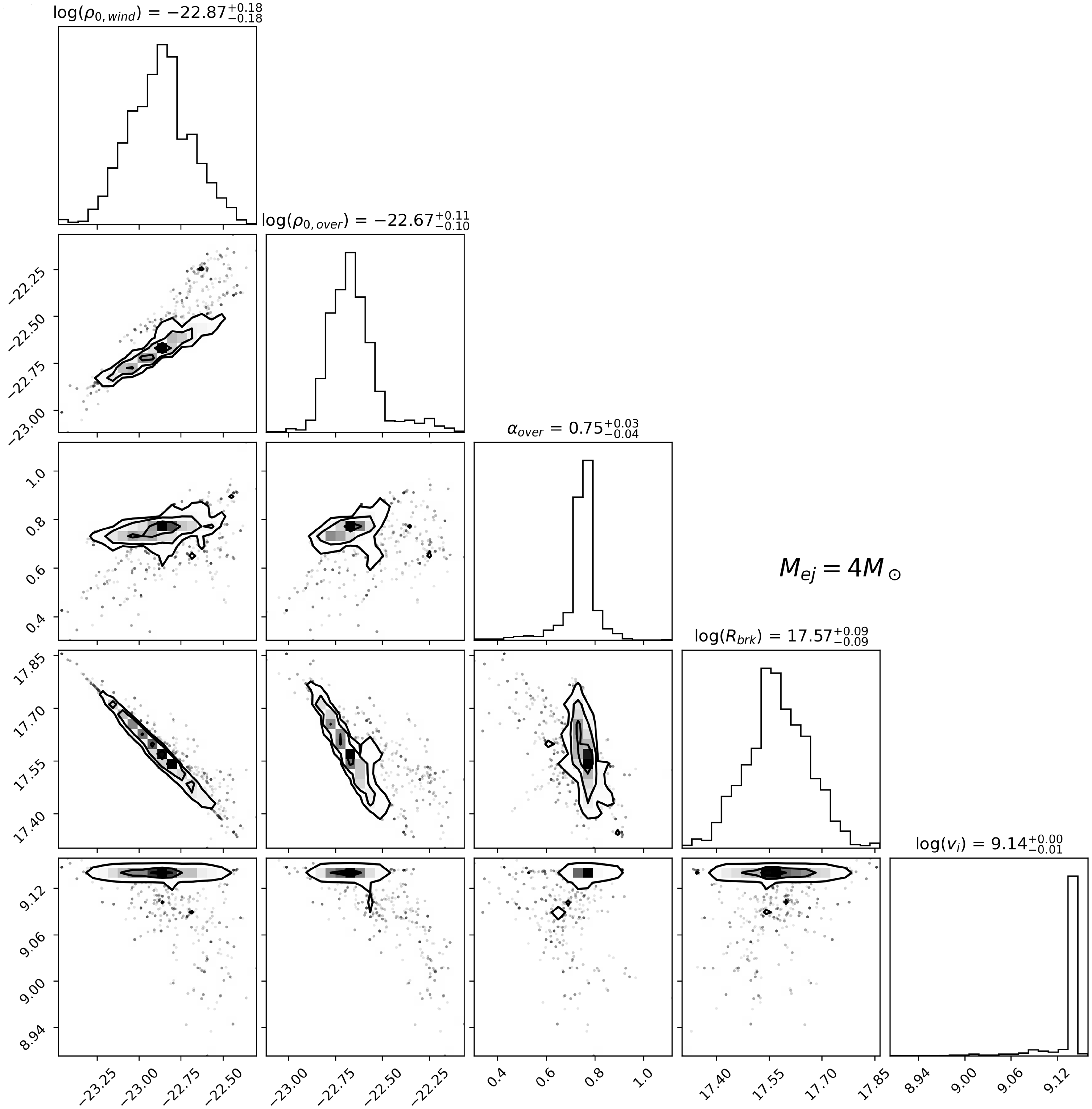
Figure A2. As in Fig. A1, for the 4 M $_\odot$
ejecta mass model. In this case, the initial shock velocity was also a fit parameter.
$_\odot$
ejecta mass model. In this case, the initial shock velocity was also a fit parameter.


 Open access