


1. Introduction
Solitary-wave solutions have been extensively investigated in the context of water-wave problems. Elevation gravity solitary waves were first observed by Scott Russell on the Edinburgh–Glasgow Union canal in 1834 (Russell Reference Russell1845). Since then, solitary waves have been observed both in nature and in laboratory experiments, and have been analysed using asymptotic and numerical methods (see, e.g. (Dauxois & Peyrard Reference Dauxois and Peyrard2006) for a recent review). Depression gravity–capillary solitary waves were observed by (Falcon, Laroche & Fauve Reference Falcon, Laroche and Fauve2002) on the surface of a thin layer of mercury. Another class of gravity–capillary solitary waves with damped oscillations has also been reported (see Longuet-Higgins Reference Longuet-Higgins1989; Vanden-Broeck & Dias Reference Vanden-Broeck and Dias1992). More recently, solitary waves have been observed experimentally and investigated numerically on liquid ferrofluid cylinders (see, for example, Blyth & Părău Reference Blyth and Părău2014).

Figure 1. Illustration of Plateau border.
Solitary-wave solutions were also predicted to propagate on Plateau borders (see Argentina et al. Reference Argentina, Cohen, Bouret, Fraysse and Raufaste2015), which are wall-free liquid microchannels that format at the junction between three bubbles or films within aqueous foams (Cantat et al. Reference Cantat, Cohen-Addad, Elias, Graner, Höhler, Pitois, Rouyer and Saint-Jalmes2013; Bouret et al. Reference Bouret, Cohen, Fraysse, Argentina and Raufaste2016). Foams are widely used in domestic and industrial applications, largely due to their high interfacial area (Whittaker & Cox Reference Whittaker and Cox2019). At equilibrium, soap films meet in threes according to Plateau’s laws, creating a microchannel known as the Plateau border (Argentina et al. Reference Argentina, Cohen, Bouret, Fraysse and Raufaste2015). The geometry of a Plateau border is very specific, as illustrated in figure 1.
In the experiments of Cohen et al. (Reference Cohen, Fraysse, Rajchenbach, Argentina, Bouret and Raufaste2014, Reference Cohen, Fraysse and Raufaste2015) Argentina et al. (Reference Argentina, Cohen, Bouret, Fraysse and Raufaste2015) and Bouret et al. (Reference Bouret, Cohen, Fraysse, Argentina and Raufaste2016) the Plateau border is inscribed within a triangular prism, and its cross-section was approximated by the tangential contact of three arcs of circles of identical radius of curvature (see also Princen Reference Princen1986). A range of physical phenomena was observed, including capillary hydraulic jumps, solitary waves, drop coalescence and inertial mass transport in Plateau borders. In particular, Cohen et al. (Reference Cohen, Fraysse, Rajchenbach, Argentina, Bouret and Raufaste2014) released droplets from above to coalesce with the Plateau border, generating capillary hydraulic jumps that propagated along the channel. Bouret et al. (Reference Bouret, Cohen, Fraysse, Argentina and Raufaste2016) injected bubbles into Plateau borders and subsequently burst them to create depression solitary waves (constrictions) that travelled at constant speed.
Typical physical parameters of the fluids used in these experiments are: viscosity $\bar {\eta }\sim 10^{-3} \,\rm N s\,m^{-2}$
, surface tension
$\bar {\eta }\sim 10^{-3} \,\rm N s\,m^{-2}$
, surface tension $\gamma \sim 4 \times 10^{-2} \,\rm N\,m^{-1}$
and density
$\gamma \sim 4 \times 10^{-2} \,\rm N\,m^{-1}$
and density $\rho \sim 10^3 \,\rm kg\,m^{-3}$
. The typical radius of curvature
$\rho \sim 10^3 \,\rm kg\,m^{-3}$
. The typical radius of curvature $a$
of the Plateau borders was
$a$
of the Plateau borders was $\sim 5 \times 10^{-4}\,\rm m$
(ranging from
$\sim 5 \times 10^{-4}\,\rm m$
(ranging from $3 \times 10^{-4} $
to
$3 \times 10^{-4} $
to $1.8 \times 10^{-3}\,\rm m$
), while their characteristic length ranged between
$1.8 \times 10^{-3}\,\rm m$
), while their characteristic length ranged between $2.5 \times 10^{-2}\,\rm $
and
$2.5 \times 10^{-2}\,\rm $
and $10^{-1}\,\rm m$
. The observed propagation speed
$10^{-1}\,\rm m$
. The observed propagation speed $c$
of solitary waves (see Bouret et al. Reference Bouret, Cohen, Fraysse, Argentina and Raufaste2016) was
$c$
of solitary waves (see Bouret et al. Reference Bouret, Cohen, Fraysse, Argentina and Raufaste2016) was $\sim\!0.2\,\rm m\,s^{-1}$
. The corresponding non-dimensional parameters are the Reynolds number
$\sim\!0.2\,\rm m\,s^{-1}$
. The corresponding non-dimensional parameters are the Reynolds number $Re$
, the Weber number
$Re$
, the Weber number $We$
and the Ohnesorge number
$We$
and the Ohnesorge number
 \begin{align} \textit{Re}=\frac {\rho c a}{\bar {\eta }}\approx 100, \quad \textit{We} = \frac {\rho c^2 a}{\gamma }\approx 0.5,\quad Oh=\frac {\sqrt {\textit{We}}}{\textit{Re}}\approx 0.007. \end{align}
Cohen et al. (Reference Cohen, Fraysse, Rajchenbach, Argentina, Bouret and Raufaste2014) and Argentina et al. (Reference Argentina, Cohen, Bouret, Fraysse and Raufaste2015) concluded that, when the Ohnesorge number satisfies $Oh=({\sqrt {\textit{We}}})/({\textit{Re}})\lt 0.05$
, the flow is inertia-dominated, allowing waves and hydraulic jumps to propagate along the Plateau border. When
$Oh=({\sqrt {\textit{We}}})/({\textit{Re}})\lt 0.05$
, the flow is inertia-dominated, allowing waves and hydraulic jumps to propagate along the Plateau border. When $Oh= ({\sqrt {\textit{We}}})/({\textit{Re}})\gt 0.05$
, viscous effects dominate and perturbations are strongly damped. In the present study, we focus on the inertia-dominated regime and leave the viscous case for a future investigation.
$Oh= ({\sqrt {\textit{We}}})/({\textit{Re}})\gt 0.05$
, viscous effects dominate and perturbations are strongly damped. In the present study, we focus on the inertia-dominated regime and leave the viscous case for a future investigation.
Previous modelling works investigating depression solitary waves and capillary jumps on Plateau borders (Argentina et al. Reference Argentina, Cohen, Bouret, Fraysse and Raufaste2015; Bouret et al. Reference Bouret, Cohen, Fraysse, Argentina and Raufaste2016; Le Doudic et al. Reference Le Doudic, Perrard and Pham2021) have employed shallow-water approximations to derive nonlinear Partial Differential Equations governing the evolution of the free surface. It is also worth noting that, in the literature, some authors have used a cylindrical coordinate system to represent the Plateau-border geometry (see, for example, (Nguyen Reference Nguyen2002). In the present study, we propose to perform a linear stability of a Plateau border subject to small perturbations, followed by the derivation of weakly nonlinear equations for waves propagating along the Plateau border, starting from the full Euler equations written in an alternative coordinate system. In particular a Korteweg–de Vries (KdV) equation will be derived to describe solitary waves, under the slender jet assumption. The long-wave approximation is justified by experimental observations showing that disturbances travelling along the Plateau border vary over length scales much larger than the local radius of curvature. This approach complements previous modelling and experimental studies.
This paper is organised as follows. Section 2 formulates the governing equation in the new non-orthogonal coordinate system. Section 3 examines the linear stability of a Plateau border to perturbations. In § 4 we derive a weakly nonlinear evolution equation for long waves on a Plateau border and a discussion is presented in § 4.
2. Problem formulation
2.1. Governing equations and boundary conditions
Consider surface-tension-driven flow of an incompressible liquid in a Plateau border with constant density $\rho$
, neglecting the effects of gravity. As mentioned in the Introduction, measurements obtained by Bouret et al. (Reference Bouret, Cohen, Fraysse, Argentina and Raufaste2016), found that the Reynolds number is large, approximately 100, hence we will assume here that the fluid is inviscid. The time scale of interest is much smaller than time scale of drainage of fluid out of the Plateau border and into the thin films (Koehler et al. Reference Koehler, Hilgenfeldt and Stone2004a
,
Reference Koehler, Hilgenfeldt and Stoneb
); therefore, we will neglect the flow out of the Plateau border and into the thin films.
$\rho$
, neglecting the effects of gravity. As mentioned in the Introduction, measurements obtained by Bouret et al. (Reference Bouret, Cohen, Fraysse, Argentina and Raufaste2016), found that the Reynolds number is large, approximately 100, hence we will assume here that the fluid is inviscid. The time scale of interest is much smaller than time scale of drainage of fluid out of the Plateau border and into the thin films (Koehler et al. Reference Koehler, Hilgenfeldt and Stone2004a
,
Reference Koehler, Hilgenfeldt and Stoneb
); therefore, we will neglect the flow out of the Plateau border and into the thin films.
We assume the flow is irrotational so that the fluid velocity is given by $\boldsymbol{u}=\boldsymbol{\nabla } \phi$
, where
$\boldsymbol{u}=\boldsymbol{\nabla } \phi$
, where $\phi (x,y,z^*,t)$
is the fluid potential,
$\phi (x,y,z^*,t)$
is the fluid potential, $(x,y,z^*)$
denote Cartesian coordinates and
$(x,y,z^*)$
denote Cartesian coordinates and $t$
is time. The
$t$
is time. The $z^*$
-axis is oriented along the direction of the flow, while the
$z^*$
-axis is oriented along the direction of the flow, while the $x$
- and
$x$
- and $y$
-axes lie in the transverse cross-section of the Plateau border. The
$y$
-axes lie in the transverse cross-section of the Plateau border. The $y$
-axis is chosen to be normal to one of the Plateau-border surfaces at the mid-point and directed outward.
$y$
-axis is chosen to be normal to one of the Plateau-border surfaces at the mid-point and directed outward.
The representation of the velocity field as a gradient of the fluid potential substituted into the incompressibility condition ( $\boldsymbol{\nabla }\boldsymbol{\cdot }\boldsymbol{u}=0$
), yields Laplace’s equation
$\boldsymbol{\nabla }\boldsymbol{\cdot }\boldsymbol{u}=0$
), yields Laplace’s equation
 \begin{align} \boldsymbol{\nabla} ^2\phi \equiv \frac {\partial ^2\phi }{\partial x^2}+\frac {\partial ^2\phi }{\partial y^2}+\frac {\partial ^2\phi }{\partial z^{*2}}=0 \ \ \ \mbox{for } x,y,z^*\in \varOmega , \end{align}
where $\varOmega$
represents the region of the Plateau border that will be defined further on. Integrating the Euler equations of motion and employing a standard vector calculus identity leads to the Bernoulli equation
$\varOmega$
represents the region of the Plateau border that will be defined further on. Integrating the Euler equations of motion and employing a standard vector calculus identity leads to the Bernoulli equation
 \begin{align} \frac {\partial \phi }{\partial t}+\frac {1}{2}|\boldsymbol{\nabla } \phi |^2+\frac {p}{\rho }=B(t) \ \ \ \mbox{for } x,y,z^*\in \varOmega , \end{align}
where $p=p(x,y,z^*,t)$
is the fluid pressure and
$p=p(x,y,z^*,t)$
is the fluid pressure and $B(t)$
is the Bernoulli constant, which in general depends on time. Since the flow is surface-tension-driven, we also have the Young–Laplace equation (Batchelor Reference Batchelor1967)
$B(t)$
is the Bernoulli constant, which in general depends on time. Since the flow is surface-tension-driven, we also have the Young–Laplace equation (Batchelor Reference Batchelor1967)
 \begin{align} p-p_0=\gamma (\boldsymbol{\nabla }\boldsymbol{\cdot }\hat {\boldsymbol{n}}), \ \ \ \mbox{for } x,y,z^*\in \partial \varOmega , \end{align}
where $p_0$
is the assumed constant air pressure outside the Plateau border which can be taken to be zero without loss of generality,
$p_0$
is the assumed constant air pressure outside the Plateau border which can be taken to be zero without loss of generality, $\partial \varOmega$
is the unknown boundary of the Plateau border to be determined,
$\partial \varOmega$
is the unknown boundary of the Plateau border to be determined, $\gamma$
is the constant surface tension coefficient and
$\gamma$
is the constant surface tension coefficient and $\hat {\boldsymbol{n}}$
is the outward-pointing unit normal to the free surface. Since both the Bernoulli equation and the Young–Laplace equation are evaluated at the boundary of
$\hat {\boldsymbol{n}}$
is the outward-pointing unit normal to the free surface. Since both the Bernoulli equation and the Young–Laplace equation are evaluated at the boundary of $\varOmega$
(i.e. the free surface), we can eliminate pressure from the Bernoulli equation, to yield
$\varOmega$
(i.e. the free surface), we can eliminate pressure from the Bernoulli equation, to yield
 \begin{align} \frac {\partial \phi }{\partial t}+\frac {1}{2}|\boldsymbol{\nabla } \phi |^2+\frac {\gamma }{\rho }(\boldsymbol{\nabla }\boldsymbol{\cdot }\hat {\boldsymbol{n}})=B(t) \ \ \ \mbox{for } x,y,z^*\in \partial \varOmega . \end{align}
A further boundary condition is required, the kinematic condition, which enforces that the normal velocity of the free surface is equal to the normal component of the fluid velocity at the free surface
 \begin{align} \boldsymbol{\nabla }\phi \boldsymbol{\cdot }\hat {\boldsymbol{n}} = \frac {\partial \boldsymbol{r}}{\partial t}\boldsymbol{\cdot }\hat {\boldsymbol{n}} \ \ \ \mbox{for } x,y,z^* \in \partial \varOmega , \end{align}
where $\boldsymbol{r}$
is position vector of a fluid particle on the free surface.
$\boldsymbol{r}$
is position vector of a fluid particle on the free surface.

Figure 2. Cross-section of a Plateau border centred at the origin $O$
.
$O$
.
2.2. Formulation of the equations of motion in the alternative coordinate system
A cross-section of a single Plateau border can be split into three equally sized regions, namely I, II and III, due to symmetry about the origin $O$
, as illustrated in figure 2. The region I is bounded by a thick circular arc with radius
$O$
, as illustrated in figure 2. The region I is bounded by a thick circular arc with radius $R(z^*,t)$
, centred at
$R(z^*,t)$
, centred at $\nu R(z^*,t)$
. Region I is separated from regions II and III by dashed straight lines on the left- and right-hand sides of the
$\nu R(z^*,t)$
. Region I is separated from regions II and III by dashed straight lines on the left- and right-hand sides of the $y$
-axis, extending from the origin to points where the cusps occur, as depicted in figure 2. The flow in regions II and III can be obtained by rotating the solution in region I by
$y$
-axis, extending from the origin to points where the cusps occur, as depicted in figure 2. The flow in regions II and III can be obtained by rotating the solution in region I by $2\pi /3$
and
$2\pi /3$
and $4\pi /3$
counter-clockwise, respectively, about the origin
$4\pi /3$
counter-clockwise, respectively, about the origin $O$
.
$O$
.

Figure 3. Coordinate system $(r,\theta )$
in the cross-section of the Plateau border at a fixed
$(r,\theta )$
in the cross-section of the Plateau border at a fixed $z$
. Note that the figure is not to scale, being dilated on the
$z$
. Note that the figure is not to scale, being dilated on the $y$
-axis. Two examples of
$y$
-axis. Two examples of $(r,\theta )$
are shown, corresponding to the cases
$(r,\theta )$
are shown, corresponding to the cases $\theta \lt \pi /2$
and
$\theta \lt \pi /2$
and $\theta \gt \pi /2$
. The positive
$\theta \gt \pi /2$
. The positive $z$
-direction points into the page.
$z$
-direction points into the page.
To describe the geometry of a Plateau border, we extend the work of Argentina et al. (Reference Argentina, Cohen, Bouret, Fraysse and Raufaste2015), which provides a parametrisation of the free surface of a Plateau border. We introduce a new coordinate system $(r,\theta ,z)$
that describes the position of a fluid particle in a Plateau border, where independent variables
$(r,\theta ,z)$
that describes the position of a fluid particle in a Plateau border, where independent variables $(r,\theta )$
are illustrated in figure 3. The
$(r,\theta )$
are illustrated in figure 3. The $z$
-axis points into the page in figure 3. The
$z$
-axis points into the page in figure 3. The $(r,\theta )$
variables describe the location of the fluid particle on a cross-sectional slice of a Plateau border, i.e. at a fixed
$(r,\theta )$
variables describe the location of the fluid particle on a cross-sectional slice of a Plateau border, i.e. at a fixed $z$
. From figure 3, we observe that
$z$
. From figure 3, we observe that
 \begin{align} x=r\cos \theta , \ \ \ y=\nu R(z,t)-r\sin \theta , \ \ \ z^*=z, \end{align}
where $\nu =2/\sqrt {3}$
(see Argentina et al. Reference Argentina, Cohen, Bouret, Fraysse and Raufaste2015 for details). We note that the origin of this coordinate system depends on
$\nu =2/\sqrt {3}$
(see Argentina et al. Reference Argentina, Cohen, Bouret, Fraysse and Raufaste2015 for details). We note that the origin of this coordinate system depends on $z$
and
$z$
and $t$
. The variable
$t$
. The variable $r$
measures the distance from the point
$r$
measures the distance from the point $\nu R(z,t)$
to a point in the Plateau border, and
$\nu R(z,t)$
to a point in the Plateau border, and $\theta$
measures the angle between the horizontal and the line subtended by the joining of the point
$\theta$
measures the angle between the horizontal and the line subtended by the joining of the point $\nu R(z,t)$
to a point in the Plateau border.
$\nu R(z,t)$
to a point in the Plateau border.
We observe that the free surface is independent of $\theta$
so that
$\theta$
so that
 \begin{align} r=R(z,t), \end{align}
defines the location of the free surface. We note that when $r=R(z,t)$
, (2.6) coincides with the parametrisation of the free surface of a Plateau border as given in Argentina et al. (Reference Argentina, Cohen, Bouret, Fraysse and Raufaste2015). From figure 3, it follows that the Cartesian variables take on the following ranges inside the Plateau border region we are considering (i.e. region I):
$r=R(z,t)$
, (2.6) coincides with the parametrisation of the free surface of a Plateau border as given in Argentina et al. (Reference Argentina, Cohen, Bouret, Fraysse and Raufaste2015). From figure 3, it follows that the Cartesian variables take on the following ranges inside the Plateau border region we are considering (i.e. region I):
 \begin{align} -\frac {R(z^*\!,t)}{2}\leqslant x \leqslant \frac {R(z^*\!,t)}{2}, \ \ \ \frac {\sqrt {3}}{3}|x| \leqslant y \leqslant \nu R(z^*\!,t)-\sqrt {R^2(z^*\!,t)-x^2}, \ \ -\infty \lt z^*\!\lt \infty . \end{align}
The inequalities (2.8) define region I of a Plateau border, and therefore, $\varOmega$
. From (2.6) and (2.8), it follows that
$\varOmega$
. From (2.6) and (2.8), it follows that $(r,\theta ,z)$
take on the following values inside region I of the Plateau border:
$(r,\theta ,z)$
take on the following values inside region I of the Plateau border:
 \begin{align} R(z,t) \leqslant r\leqslant \nu R(z,t), \ \ \ \ \frac {\pi }{3}\leqslant \theta \leqslant \frac {2\pi }{3}, \ \ \ \ -\infty \lt z\lt \infty . \end{align}
We define the $(r,\theta ,z)$
in the coordinate system for the Plateau border as
$(r,\theta ,z)$
in the coordinate system for the Plateau border as
 \begin{align} r&=\sqrt {x^2+(y-\nu R(z^*,t))^2}, \end{align}
 \begin{align} \theta &= \left \{\begin{array}{ccc} \arctan\! \left(\dfrac {\nu R(z^*,t)-y}{x} \right) & : & x\gt 0 ,\\[6pt] \dfrac {\pi }{2} & : & x=0, \\[6pt] \pi +\arctan\! \left( \dfrac {\nu R(z^*,t)-y}{x} \right) & : & x\lt 0, \end{array} \right . \end{align}
 \begin{align} z &=z^*, \end{align}
where $r\gt 0$
since it is a measure of distance. We note that
$r\gt 0$
since it is a measure of distance. We note that $\nu R(z^*,t)-y\gt 0$
in region I of the Plateau border, and thus from (2.11) it can be seen that
$\nu R(z^*,t)-y\gt 0$
in region I of the Plateau border, and thus from (2.11) it can be seen that $\theta$
is continuous at
$\theta$
is continuous at $x=0$
. Moreover, it can be shown that
$x=0$
. Moreover, it can be shown that $\theta$
is differentiable at
$\theta$
is differentiable at $x=0$
by considering limits.
$x=0$
by considering limits.
The position, $\boldsymbol{r}$
, of a fluid element in the Plateau border is defined by the coordinates
$\boldsymbol{r}$
, of a fluid element in the Plateau border is defined by the coordinates $(r,\theta ,z)\equiv (x^1,x^2,x^3)$
as
$(r,\theta ,z)\equiv (x^1,x^2,x^3)$
as
 \begin{align} \boldsymbol{r}(r,\theta ,z)=r\cos \theta \hat {\boldsymbol{i}}+(R(z,t)\nu -r\sin \theta )\hat {\!\boldsymbol{j}}+z\hat {\boldsymbol{k}}, \end{align}
where $\hat {\boldsymbol{i}},\hat {\!\boldsymbol{j}},\hat {\boldsymbol{k}}$
are the Cartesian basis vectors pointing in the positive
$\hat {\boldsymbol{i}},\hat {\!\boldsymbol{j}},\hat {\boldsymbol{k}}$
are the Cartesian basis vectors pointing in the positive $x,y,z^*$
directions, respectively. The basis vectors are (see Simmonds Reference Simmonds2012)
$x,y,z^*$
directions, respectively. The basis vectors are (see Simmonds Reference Simmonds2012) $\boldsymbol{e}_i= {\partial \boldsymbol{r}}/{\partial x^i}$
, i.e.
$\boldsymbol{e}_i= {\partial \boldsymbol{r}}/{\partial x^i}$
, i.e.
 \begin{align} \boldsymbol{e}_1 &\equiv \boldsymbol{e}_r =\frac {\partial \boldsymbol{r}}{\partial r}=\cos \theta \hat {\boldsymbol{i}}-\sin \theta \hat {\!\boldsymbol{j}},\\[-6pt] \nonumber \end{align}
 \begin{align} \boldsymbol{e}_2 & \equiv \boldsymbol{e}_{\theta }=\frac {\partial \boldsymbol{r}}{\partial \theta }=-r\sin \theta \hat {\boldsymbol{i}}-r\cos \theta \hat {\!\boldsymbol{j}},\\[-6pt] \nonumber \end{align}
 \begin{align} \boldsymbol{e}_3 & \equiv \boldsymbol{e}_{z}=\frac {\partial \boldsymbol{r}}{\partial z}=\nu \frac {\partial \!R}{\partial z}\hat {\!\boldsymbol{j}}+\hat {\boldsymbol{k}}, \\[9pt] \nonumber \end{align}
which are neither all orthogonal nor all unit vectors. We note that there is a similarity between the alternative coordinate system $(r,\theta ,z)$
and a cylindrical coordinate system, as seen from (2.14) and (2.15), except
$(r,\theta ,z)$
and a cylindrical coordinate system, as seen from (2.14) and (2.15), except $\boldsymbol{e}_z\neq \hat {\boldsymbol{k}}$
. Is is also worth noting that they can be normalised as
$\boldsymbol{e}_z\neq \hat {\boldsymbol{k}}$
. Is is also worth noting that they can be normalised as
 \begin{align} \boldsymbol{\hat {e}}_r = \boldsymbol{e}_r , \quad \boldsymbol{\hat {e}}_\theta = \frac {\boldsymbol{e}_{\theta }}{r}, \quad \boldsymbol{\hat {e}}_z =\frac {\boldsymbol{e}_{z}}{\sqrt {\left (\nu \dfrac {\partial\! R}{\partial z}\right )^{\!2}+1}}. \end{align}
The corresponding inverse relations to (2.14)–(2.16) are
 \begin{align} \hat {\boldsymbol{i}} & = \cos \theta \boldsymbol{e}_r-\frac {\sin \theta }{r}\boldsymbol{e}_{\theta },\\[-12pt]\nonumber \end{align}
 \begin{align} \hat {\!\boldsymbol{j}} & = -\sin \theta \boldsymbol{e}_r-\frac {\cos \theta }{r}\boldsymbol{e}_{\theta },\\[-12pt]\nonumber \end{align}
 \begin{align} \hat {\boldsymbol{k}} & =\nu \sin \theta \frac {\partial\! R}{\partial z}\boldsymbol{e}_r+\frac {\nu \cos \theta }{r}\frac {\partial\! R}{\partial z}\boldsymbol{e}_{\theta }+\boldsymbol{e}_z. \\[9pt] \nonumber \end{align}
Using the multi-variable chain rule and (A1) from Appendix A, Laplace’s equation (2.1) becomes
 \begin{align} \boldsymbol{\nabla} ^2\phi = & \frac {\partial ^2\phi }{\partial r^2}+\frac {1}{r}\frac {\partial \phi }{\partial r}+\frac {1}{r^2}\frac {\partial ^2 \phi }{\partial \theta ^2}+\frac {\partial ^2\phi }{\partial z^2} \notag \\ & +\frac {\partial ^2\phi }{\partial r^2}\left ( \frac {\partial\! R}{\partial z}\right )^{\!2}\nu ^2\sin ^2\theta +\frac {\partial ^2\phi }{\partial r\partial \theta }\!\left (\frac {\partial\! R}{\partial z}\right )^{\!2}\frac {2\nu ^2\cos \theta \sin \theta }{r}+\frac {\partial \phi }{\partial r}\!\left ( \frac {\partial\! R}{\partial z}\right )^{\!2}\!\frac {\nu ^2\cos ^2\theta }{r} \notag \\ & -2\frac {\partial \phi }{\partial \theta }\left ( \frac {\partial\! R}{\partial z}\right )^{\!2}\frac {\nu ^2\sin \theta \cos \theta }{r^2}+\frac {\partial ^2\phi }{\partial \theta ^2}\left ( \frac {\partial\! R}{\partial z} \right )^{\!2}\frac {\nu ^2\cos ^2\theta }{r^2}+2\frac {\partial ^2\phi }{\partial z\partial r}\frac {\partial\! R}{\partial z}\nu \sin \theta \notag \\ & +\frac {\partial \phi }{\partial r}\frac {\partial ^2R}{\partial z^2}\nu \sin \theta +2\frac {\partial ^2\phi }{\partial z\partial \theta }\frac {\partial\! R}{\partial z}\frac {\nu \cos \theta }{r}+\frac {\partial \phi }{\partial \theta }\frac {\partial ^2R}{\partial z^2}\frac {\nu \cos \theta }{r}=0, \ \ \ \notag \\ & \mbox{for } \ \ \ R(z,t)\leqslant r \leqslant \nu R(z,t), \ \ \frac {\pi }{3}\leqslant \theta \leqslant \frac {2\pi }{3}, \ \ \mbox{and} \ -\infty \lt z\lt \infty . \end{align}
The $|\boldsymbol{\nabla }\phi |^2$
term appearing in the Bernoulli condition (2.4) is more easily calculated in the Cartesian basis vectors. Thus, from (A1), we have
$|\boldsymbol{\nabla }\phi |^2$
term appearing in the Bernoulli condition (2.4) is more easily calculated in the Cartesian basis vectors. Thus, from (A1), we have
 \begin{align} \boldsymbol{\nabla }\phi &\equiv \frac {\partial \phi }{\partial x}\hat {\boldsymbol{i}}+\frac {\partial \phi }{\partial y}\skew 2\hat {\!\boldsymbol{j}}+\frac {\partial \phi }{\partial z^*}\hat {\boldsymbol{k}} \notag \\ &= \left ( \cos \theta \frac {\partial \phi }{\partial r}-\frac {\sin \theta }{r}\frac {\partial \phi }{\partial \theta } \right )\!\hat {\boldsymbol{i}}+\left (-\sin \theta \frac {\partial \phi }{\partial r}-\frac {\cos \theta }{r}\frac {\partial \phi }{\partial \theta } \right )\!\skew 2\hat {\!\boldsymbol{j}} \notag \\ & \quad +\left (\nu \sin \theta \frac {\partial\! R}{\partial z}\frac {\partial \phi }{\partial r}+\frac {\nu \cos \theta }{r}\frac {\partial r}{\partial z}\frac {\partial \phi }{\partial \theta }+\frac {\partial \phi }{\partial z} \right )\!\hat {\boldsymbol{k}}. \end{align}
Using (2.22), $|\boldsymbol{\nabla }\phi |^2$
is given by
$|\boldsymbol{\nabla }\phi |^2$
is given by
 \begin{align} |\boldsymbol{\nabla }\phi |^2 &= \left ( \frac {\partial \phi }{\partial r}\right )^{\!2}+\frac {1}{r^2}\left ( \frac {\partial \phi }{\partial \theta }\right )^{\!2}+\left ( \frac {\partial\! R}{\partial z}\right )^{\!2}\left (\frac {\partial \phi }{\partial r}\right )^{\!2}\nu ^2\sin ^2\theta +\left (\frac {\partial\! R}{\partial z}\right )^{\!2} \left (\frac {\partial \phi }{\partial \theta }\right )^{\!2}\frac {\nu ^2\cos ^2\theta }{r^2} \notag \\ &\quad +\left (\frac {\partial \phi }{\partial z}\right )^{\!2} +\frac {2\nu ^2\cos \theta \sin \theta }{r}\left ( \frac {\partial\! R}{\partial z}\right )^{\!2}\frac {\partial \phi }{\partial r}\frac {\partial \phi }{\partial \theta }+2\nu \sin \theta \frac {\partial\! R}{\partial z}\frac {\partial \phi }{\partial r}\frac {\partial \phi }{\partial z} \notag \\ &\quad +\frac {2\nu \cos \theta }{r}\frac {\partial\! R}{\partial z}\frac {\partial \phi }{\partial \theta }\frac {\partial \phi }{\partial z}. \end{align}
2.3. Curvature of the free surface
The material surface that defines the free surface of a Plateau border is
 \begin{align} F(x,y,z^*,t)\equiv R(z^*,t)^2-x^2-(y-\nu R(z^*,t))^2=0. \end{align}
Hence the outward-pointing unit normal vector is
 \begin{align} \hat {\boldsymbol{n}}= \frac {\boldsymbol{\nabla } F}{|\boldsymbol{\nabla } F|}= \dfrac {{-}\cos \theta \hat {\boldsymbol{i}}+\sin \theta \skew 2\hat {\!\boldsymbol{j}}-\dfrac {\partial\! R}{\partial z}(\nu \sin \theta -1)\hat {\boldsymbol{k}} }{\sqrt {1+\left (\dfrac {\partial\! R}{\partial z} \right )^{\!2}(\nu \sin \theta -1)^2}},\end{align}
and its divergence is, after some algebra,
 \begin{align} \boldsymbol{\nabla }\boldsymbol{\cdot }\hat {\boldsymbol{n}} =\dfrac {(1-\nu \sin \theta )\dfrac {\partial ^2R}{\partial z^2}R-1+(2\nu \sin \theta -\nu ^2-1)\left (\dfrac {\partial\! R}{\partial z}\right )^{\!2}}{R\Bigg [1+(\nu \sin \theta -1)^2\left ( \dfrac {\partial\! R}{\partial z}\right )^{\!2}\Bigg ]^{3/2}}. \end{align}
The Bernoulli condition, after substituting (2.26) and (2.23) into (2.4), is
 \begin{align} &\frac {\partial \phi }{\partial t}+\frac {1}{2}\Bigg (\! \left ( \frac {\partial \phi }{\partial r}\right )^{\!2}+\frac {1}{r^2}\left ( \frac {\partial \phi }{\partial \theta }\right )^{\!2}+\left ( \frac {\partial\! R}{\partial z}\frac {\partial \phi }{\partial r}\right )^{\!2}\nu ^2\sin ^2\theta +\left (\frac {\partial\! R}{\partial z}\right )^{\!2} \left (\frac {\partial \phi }{\partial \theta }\right )^{\!2}\frac {\nu ^2\cos ^2\theta }{r^2} \notag \\ & +\left (\frac {\partial \phi }{\partial z}\right )^{\!2} +\frac {2\nu ^2\cos \theta \sin \theta }{r}\left ( \frac {\partial\! R}{\partial z}\right )^{\!2}\frac {\partial \phi }{\partial r}\frac {\partial \phi }{\partial \theta }+2\nu \sin \theta \frac {\partial\! R}{\partial z}\frac {\partial \phi }{\partial r}\frac {\partial \phi }{\partial z}+\frac {2\nu \cos \theta }{r}\frac {\partial\! R}{\partial z}\frac {\partial \phi }{\partial \theta }\frac {\partial \phi }{\partial z}\! \Bigg ) \notag \\ & +\frac {\gamma }{\rho }\left (\dfrac {(1-\nu \sin \theta )\dfrac {\partial ^2R}{\partial z^2}R-1+(2\nu \sin \theta -\nu ^2-1)\left (\dfrac {\partial\! R}{\partial z}\right )^{\!2}}{R\Bigg [1+(\nu \sin \theta -1)^2\left ( \dfrac {\partial\! R}{\partial z}\right )^{\!2}\Bigg ]^{3/2}} \right )=B(t), \end{align}
on $r=R(z,t)$
.
$r=R(z,t)$
.
2.4. Kinematic boundary condition
We note from (2.13) that $ {\partial \boldsymbol{r}}/{\partial t}$
, where
$ {\partial \boldsymbol{r}}/{\partial t}$
, where $\boldsymbol{r}$
is the position of the fluid particle on the free surface, is given by
$\boldsymbol{r}$
is the position of the fluid particle on the free surface, is given by
 \begin{align} \frac {\partial \boldsymbol{r}}{\partial t}=\frac {\partial\! R}{\partial t}\cos \theta \hat {\boldsymbol{i}}+\frac {\partial\! R}{\partial t}(\nu -\sin \theta )\skew 2\hat {\!\boldsymbol{j}}. \end{align}
From (2.22), (2.25) and (2.28) the kinematic boundary condition (2.5) becomes, after some algebra,
 \begin{align} & \frac {\partial\! R}{\partial t}(1-\nu \sin \theta )-\frac {\partial \phi }{\partial r} \notag \\ & \ \ \ \ +\frac {\partial\! R}{\partial z}(1-\nu \sin \theta )\left (\nu \sin \theta \frac {\partial\! R}{\partial z}\frac {\partial \phi }{\partial r}+\frac {\nu \cos \theta }{r}\frac {\partial\! R}{\partial z}\frac {\partial \phi }{\partial \theta }+\frac {\partial \phi }{\partial z}\right )=0 \ \ \ \mbox{on } r=R(z,t). \end{align}
2.5. Symmetry boundary condition
To establish another boundary condition, consider a cross-sectional slice of a Plateau border. Imagine the fluid velocity vector at the origin $O$
, pointing radially outwards (in the
$O$
, pointing radially outwards (in the $\boldsymbol{e}_r$
direction). If the velocity vector has non-zero components in the
$\boldsymbol{e}_r$
direction). If the velocity vector has non-zero components in the $\hat {\boldsymbol{i}}$
and
$\hat {\boldsymbol{i}}$
and $\skew 2\hat {\!\boldsymbol{j}}$
directions, rotating the cross-section of the Plateau border by integer multiples of
$\skew 2\hat {\!\boldsymbol{j}}$
directions, rotating the cross-section of the Plateau border by integer multiples of $2\pi /3$
would lead to an inconsistency. By symmetry, the fluid velocity of the Plateau border must be identical to the fluid velocity of the rotated Plateau border. The only way to satisfy this for any integer multiple of
$2\pi /3$
would lead to an inconsistency. By symmetry, the fluid velocity of the Plateau border must be identical to the fluid velocity of the rotated Plateau border. The only way to satisfy this for any integer multiple of $2\pi /3$
is if the components of fluid velocity vector in
$2\pi /3$
is if the components of fluid velocity vector in $\hat {\boldsymbol{i}}$
and
$\hat {\boldsymbol{i}}$
and $\skew 2\hat {\!\boldsymbol{j}}$
directions at the origin are zero. Mathematically, this means
$\skew 2\hat {\!\boldsymbol{j}}$
directions at the origin are zero. Mathematically, this means
 \begin{align} \boldsymbol{u}\boldsymbol{\cdot } \hat {\boldsymbol{i}}=0, \ \ \ \mbox{and } \boldsymbol{u}\boldsymbol{\cdot }\skew 2\hat {\!\boldsymbol{j}}=0, \ \ \ \ \mbox{on } r=\nu R(z,t), \end{align}
where the origin $O$
is defined by
$O$
is defined by $r=\nu R(z,t)$
in region I of the Plateau border. The fluid velocity vector in the alternative coordinate system, expressed in terms of the
$r=\nu R(z,t)$
in region I of the Plateau border. The fluid velocity vector in the alternative coordinate system, expressed in terms of the $\{\boldsymbol{e}_r,\boldsymbol{e}_{\theta },\boldsymbol{e}_z\}$
vectors, is
$\{\boldsymbol{e}_r,\boldsymbol{e}_{\theta },\boldsymbol{e}_z\}$
vectors, is
 \begin{align} \boldsymbol{u}=u^r\boldsymbol{e}_r+u^{\theta }\boldsymbol{e}_{\theta }+u^z\boldsymbol{e}_z, \end{align}
where $u^r,u^{\theta },u^z$
are the velocity components in the
$u^r,u^{\theta },u^z$
are the velocity components in the $\boldsymbol{e}_r,\boldsymbol{e}_{\theta }$
and
$\boldsymbol{e}_r,\boldsymbol{e}_{\theta }$
and $\boldsymbol{e}_z$
directions, respectively.
$\boldsymbol{e}_z$
directions, respectively.
After some work (see Appendix A) we find that the symmetry condition at $r=\nu R(z,t)$
is given by
$r=\nu R(z,t)$
is given by
 \begin{align} u^r\cos \theta -u^{\theta }r\sin \theta =0, \ \ \ \ \mbox{and } \ \ \ {-}u^r\sin \theta -u^{\theta }r\cos \theta +\nu \frac {\partial\! R}{\partial z}u^z=0. \end{align}
To determine the components of the fluid velocity in terms of the fluid potential, we substitute (2.18)–(2.20) into (2.22), to obtain
 \begin{align} u^r & =\left (1+\left (\frac {\partial\! R}{\partial z}\right )^{\!2}\nu ^2\sin ^2\theta \right )\frac {\partial \phi }{\partial r}+\frac {\nu ^2\cos \theta \sin \theta }{r}\left (\frac {\partial\! R}{\partial z} \right )^{\!2}\frac {\partial \phi }{\partial \theta }+\nu \sin \theta \frac {\partial\! R}{\partial z}\frac {\partial \phi }{\partial z}, \end{align}
 \begin{align} u^{\theta } & =\frac {\nu ^2\cos \theta \sin \theta }{r}\left (\frac {\partial\! R}{\partial z} \right )^{\!2}\frac {\partial \phi }{\partial r}+\frac {1}{r^2}\left (1+\left ( \frac {\partial\! R}{\partial z} \right )^{\!2}\nu ^2\cos ^2\theta \right )^{\!2}\frac {\partial \phi }{\partial \theta } +\frac {\nu \cos \theta }{r}\frac {\partial\! R}{\partial z}\frac {\partial \phi }{\partial z}, \end{align}
 \begin{align} u^z & =\nu \sin \theta \frac {\partial\! R}{\partial z}\frac {\partial \phi }{\partial r}+\frac {\nu \cos \theta }{r}\frac {\partial\! R}{\partial z}\frac {\partial \phi }{\partial \theta }+\frac {\partial \phi }{\partial z}. \end{align}
The symmetry condition expressed in terms of the fluid potential, after substituting (2.33)–(2.35) into the symmetry condition (2.32), is
 \begin{align} \frac {\partial \phi }{\partial r}\cos \theta -\frac {1}{r}\frac {\partial \phi }{\partial \theta }\sin \theta =0, \quad \mathrm{and} \quad \frac {\partial \phi }{\partial r}\sin \theta +\frac {1}{r}\frac {\partial \phi }{\partial \theta }\cos \theta =0, \ \ \ \ \mbox{on } r=\nu R(z,t). \end{align}
This completes the derivation of the boundary conditions.
3. Linear stability analysis
Following Argentina et al. (Reference Argentina, Cohen, Bouret, Fraysse and Raufaste2015), we perform azimuthal averaging over a given cross-section of the Plateau border. This means we take $\theta =\pi /2$
. Due to this averaging, we assume the fluid velocity component in the azimuthal direction,
$\theta =\pi /2$
. Due to this averaging, we assume the fluid velocity component in the azimuthal direction, $u^{\theta }$
, is zero everywhere on
$u^{\theta }$
, is zero everywhere on $\theta =\pi /2$
. Furthermore, we assume that all variables are independent of
$\theta =\pi /2$
. Furthermore, we assume that all variables are independent of $\theta$
. This effectively reduces a three-dimensional problem to a two-dimensional one. Henceforth, in this section, we assume
$\theta$
. This effectively reduces a three-dimensional problem to a two-dimensional one. Henceforth, in this section, we assume
 \begin{align} \theta =\frac {\pi }{2} \ \ \mbox{and } u^{\theta }=0, \ \ \frac {\partial }{\partial \theta }=0 \ \ \ \mbox{on } \theta =\frac {\pi }{2}. \end{align}
We consider the Plateau border to be in a uniform state, meaning the $r$
-variable is a constant,
$r$
-variable is a constant, $r=a$
. Substituting
$r=a$
. Substituting $r=a$
into the Young–Laplace (2.3) we find the basic state pressure to be
$r=a$
into the Young–Laplace (2.3) we find the basic state pressure to be $p=-\gamma /a$
. We also assume the Plateau border to be stationary, so we define the basic state (denoted with overbars) as
$p=-\gamma /a$
. We also assume the Plateau border to be stationary, so we define the basic state (denoted with overbars) as
 \begin{align} \bar {\phi }=0, \ \ \ \ \bar {p}=-\frac {\gamma }{a}, \ \ \ \ \bar {R}=a. \end{align}
We perturb this uniform Plateau border by adding small disturbances, scaled by $\epsilon$
, where
$\epsilon$
, where $\epsilon$
represents the characteristic ratio between the amplitude of a wave to its wavelength and we assume
$\epsilon$
represents the characteristic ratio between the amplitude of a wave to its wavelength and we assume $0\lt \epsilon \ll 1$
. Hence, we write
$0\lt \epsilon \ll 1$
. Hence, we write
 \begin{align} \phi (r,z,t)=\epsilon \hat {\phi }(r,z,t)+O(\epsilon ^2), \ \ \ \ \ R(z,t)=\bar {R}+\epsilon \hat {\eta }(z,t)+O(\epsilon ^2), \ \ \ \end{align}
where the hat decoration denote perturbation quantities. Note that, once the solution for $\hat {\phi }(r,z,t)$
is found, the pressure field can be determined from the Bernoulli equation (2.2). Substituting the exact basic state solution (3.2) into the Bernoulli equation we find the Bernoulli constant to be
$\hat {\phi }(r,z,t)$
is found, the pressure field can be determined from the Bernoulli equation (2.2). Substituting the exact basic state solution (3.2) into the Bernoulli equation we find the Bernoulli constant to be $B(t)=-\gamma /(\rho a)$
. We substitute (3.3) into the governing Laplace equation (2.21) and the boundary conditions: the Bernoulli condition (2.27), the kinematic condition (2.29) and the symmetry condition (2.36). After performing Taylor expansions of the boundary conditions about
$B(t)=-\gamma /(\rho a)$
. We substitute (3.3) into the governing Laplace equation (2.21) and the boundary conditions: the Bernoulli condition (2.27), the kinematic condition (2.29) and the symmetry condition (2.36). After performing Taylor expansions of the boundary conditions about $r=a$
for Bernoulli and kinematic, and about
$r=a$
for Bernoulli and kinematic, and about $r=a\nu$
for the symmetry condition, and then neglecting terms of
$r=a\nu$
for the symmetry condition, and then neglecting terms of $O(\epsilon ^2)$
and higher, we obtain the linearised equations of motion at
$O(\epsilon ^2)$
and higher, we obtain the linearised equations of motion at $O(\epsilon )$
 \begin{align} \frac {\partial ^2\hat {\phi }}{\partial r^2}+\frac {1}{r}\frac {\partial \hat {\phi }}{\partial r}+\frac {\partial ^2\hat {\phi }}{\partial z^2}&=0 \ \ \ \ && \mbox{for } a\leqslant r\leqslant a\nu , \end{align}
 \begin{align} \frac {\partial \hat {\eta }}{\partial t}(1-\nu )-\frac {\partial \hat {\phi }}{\partial r}& =0 \ \ \ \ && \mbox{on } r=a, \end{align}
 \begin{align} \frac {\partial \hat {\phi }}{\partial t}+\frac {\gamma }{\rho }\left ( (1-\nu )\frac {\partial ^2\hat {\eta }}{\partial z^2}+\frac {\hat {\eta }}{a^2} \right ) & =0 \ \ \ \ && \mbox{on } r=a, \end{align}
 \begin{align} \frac {\partial \hat {\phi }}{\partial r} & =0 \ \ \ \ && \mbox{on } r=a\nu . \end{align}
We seek a solution for these linearised equations of motion that is periodic in $z$
and exponential in
$z$
and exponential in $t$
. Specifically, we look for solutions of the form
$t$
. Specifically, we look for solutions of the form
 \begin{align} \hat {\phi }(r,z,t) &=\varPhi (r)\exp ({i}kz+st)+\mathrm{c.c.}, \ \ \ \ \hat {\eta }(z,t)=\hat {\eta }_0\exp ({i}kz+st)+{c.c.}, \end{align}
where $\hat {\eta }_0$
is a constant,
$\hat {\eta }_0$
is a constant, $\mathrm{c.c.}$
denotes the complex conjugate of the preceding part of the equation (this convention applies throughout the rest of the text, but will not be explicitly stated again). Here,
$\mathrm{c.c.}$
denotes the complex conjugate of the preceding part of the equation (this convention applies throughout the rest of the text, but will not be explicitly stated again). Here, $k$
is the real and positive wavenumber, and
$k$
is the real and positive wavenumber, and $s$
is the temporal growth rate. If
$s$
is the temporal growth rate. If $s\in {i}\mathbb{R}$
(purely imaginary), then waves will emerge on the free surface of the Plateau border. If
$s\in {i}\mathbb{R}$
(purely imaginary), then waves will emerge on the free surface of the Plateau border. If $s\in \mathbb{R}^{\gt 0}$
(real and positive), the flow is unstable and will diverge from the basic state. If
$s\in \mathbb{R}^{\gt 0}$
(real and positive), the flow is unstable and will diverge from the basic state. If $s\in \mathbb{R}^{\leqslant 0}$
(real and non-positive), the flow is stable and, after a sufficiently long time, the perturbations will decay and the flow will return to the basic state.
$s\in \mathbb{R}^{\leqslant 0}$
(real and non-positive), the flow is stable and, after a sufficiently long time, the perturbations will decay and the flow will return to the basic state.
Substituting (3.8) into (3.4), we find that $\varPhi (r)$
satisfies
$\varPhi (r)$
satisfies
 \begin{align} \frac {{\rm d}^2\varPhi }{{\rm d} r^2}+\frac {1}{r}\frac {{\rm d} \varPhi }{{\rm d} r}-k^2\varPhi =0, \end{align}
which is Bessel’s modified equation of zeroth order. It has two linearly independent solutions: ${I}_0$
and
${I}_0$
and ${K}_0$
, known as the modified Bessel functions of the first and second kinds, both of zeroth order, respectively. It is well known (see, for example, Olver Reference Olver2010) that modified Bessel function
${K}_0$
, known as the modified Bessel functions of the first and second kinds, both of zeroth order, respectively. It is well known (see, for example, Olver Reference Olver2010) that modified Bessel function ${I}_n$
(modified Bessel function of the first kind of order
${I}_n$
(modified Bessel function of the first kind of order $n$
) is finite at the origin and grow exponentially with a singularity at infinity, while
$n$
) is finite at the origin and grow exponentially with a singularity at infinity, while ${K}_n$
(modified Bessel function of the second kind of order
${K}_n$
(modified Bessel function of the second kind of order $n$
) is singular at the origin and decays exponentially. Therefore, both
$n$
) is singular at the origin and decays exponentially. Therefore, both ${I}_n(\textit{kr})$
and
${I}_n(\textit{kr})$
and ${K}_n(\textit{kr})$
remain finite within the Plateau border (
${K}_n(\textit{kr})$
remain finite within the Plateau border ( $a\leqslant r\leqslant a\nu$
). Thus, (3.9) has the general solution
$a\leqslant r\leqslant a\nu$
). Thus, (3.9) has the general solution
 \begin{align} \varPhi (r)=C_1{I}_0(\textit{kr})+C_2{K}_0(\textit{kr}), \end{align}
where $C_1,C_2$
are arbitrary constants of integration. We have three unknown constants
$C_1,C_2$
are arbitrary constants of integration. We have three unknown constants $C_1,C_2$
and
$C_1,C_2$
and $\hat {\eta }_0$
, and therefore require three boundary conditions. Applying the symmetry condition (2.36) to (3.10), we find
$\hat {\eta }_0$
, and therefore require three boundary conditions. Applying the symmetry condition (2.36) to (3.10), we find
 \begin{align} \varPhi (r)=C_1\left ({I}_0(\textit{kr})+\frac {{I}_1(k\nu a)}{{K}_1(k\nu a)}{K}_0(\textit{kr}) \right )\!. \end{align}
We express the kinematic (3.5) and Bernoulli conditions (3.6) in matrix-vector form as
 \begin{align} \left ( \!\!\begin{array}{cc} -k\!\left ({I}_1(ka)-\dfrac {{I}_1(k\nu a)}{{K}_1(k\nu a)}{K}_1(ka) \right ) & s(1-\nu ) \\[6pt] s\!\left ({I}_0(\textit{kr})+\dfrac {{I}_1(k\nu a)}{{K}_1(k\nu a)}{K}_0(\textit{kr}) \right ) & \dfrac {\gamma }{\rho }\left (\dfrac {1}{a^2}-(1-\nu )k^2 \right ) \end{array} \!\!\right )\left ( \!\!\begin{array}{c} C_1 \\ \hat {\eta }_0 \end{array} \!\!\right )=\left (\!\!\begin{array}{c} 0 \\ 0 \end{array} \!\!\right )\!. \end{align}
The first and second rows correspond to the kinematic and Bernoulli conditions, respectively. For this matrix-vector (3.12) to admit a non-trivial solution, we require that the determinant of the matrix vanishes, which yields
 \begin{align} s^2= -\frac {\gamma (ka)}{\rho a^3}\left [\frac {1}{1-\nu }-(ak)^2 \right ]\frac { {I}_1(ka){K}_1(k\nu a)-{I}_1(k\nu a){K}_1(ka)}{{I}_0(ka){K}_1(k\nu a)+{I}_1(k\nu a){K}_0(ka)} . \end{align}
This is the linear inviscid dispersion relation for a Plateau border with azimuthal averaging. We observe the term in the square brackets in the dispersion relation, (3.13), is negative for all real $k$
. To analysis the stability of the Plateau border, we need to determine the sign of
$k$
. To analysis the stability of the Plateau border, we need to determine the sign of
 \begin{align} \varLambda :=\frac { {I}_1(ka){K}_1(k\nu a)-{I}_1(k\nu a){K}_1(ka)}{{I}_0(ka){K}_1(k\nu a)+{I}_1(k\nu a){K}_0(ka)}. \end{align}
We note the following inequalities for the modified Bessel functions (see, for example, Radwan Reference Radwan1992; Olver Reference Olver2010, p. 5):
 \begin{align} |{K}_1(\xi q)|&\gt |{K}_1(\xi )|, \end{align}
 \begin{align} {I}_1(\xi q) &\lt {I}_1(\xi ). \end{align}
It is well known that $ I_n(z),{K}_n(z)$
are positive for non-negative arguments; thus, the denominator of (3.14) is positive for all
$ I_n(z),{K}_n(z)$
are positive for non-negative arguments; thus, the denominator of (3.14) is positive for all $ka\geqslant 0$
. If we define
$ka\geqslant 0$
. If we define $\xi =k\nu a$
and
$\xi =k\nu a$
and $q={1}/{\nu }$
such that
$q={1}/{\nu }$
such that $0\lt q\lt 1$
, then since
$0\lt q\lt 1$
, then since
 \begin{align} \frac {{I}_1(\xi ){K}_1(\xi q)}{{I}_1(\xi q){K}_1(\xi )}\gt 1, \end{align}
it follows that the numerator of (3.14) is negative for all $ka\geqslant 0$
. Consequently,
$ka\geqslant 0$
. Consequently, $\varLambda \lt 0$
for all
$\varLambda \lt 0$
for all $ka\geqslant 0$
which implies
$ka\geqslant 0$
which implies $s\in {i}\mathbb{R}$
and the Plateau border is stable for all real and positive wavenumbers.
$s\in {i}\mathbb{R}$
and the Plateau border is stable for all real and positive wavenumbers.
3.1. Non-dimensionalisation and long-wave speed
We now derive the non-dimensional dispersion relation by non-dimensionalising all lengths in units of the unperturbed $r$
-coordinate,
$r$
-coordinate, $a$
. We perform the non-dimensionalisation as follows:
$a$
. We perform the non-dimensionalisation as follows:
 \begin{align} r=ar', \ \ \ \ z=az', \ \ \ \ t=\sqrt {\frac {a^3\rho }{\gamma }}t', \end{align}
where primed quantities denote non-dimensional ones. Substituting (3.18) into (3.13), we obtain the non-dimensional dispersion relation
 \begin{align} s^2=-k\left ( \frac {1}{1-\nu }-k^2 \right )\frac { {I}_1(k){K}_1(k\nu )-{I}_1(k\nu ){K}_1(k)}{{I}_0(k){K}_1(k\nu )+{I}_1(k\nu ){K}_0(k)}. \end{align}
By writing $s=-\mathrm{i}kc$
, where
$s=-\mathrm{i}kc$
, where $c$
is the phase speed of the wave, and substituting in (3.19) we obtain
$c$
is the phase speed of the wave, and substituting in (3.19) we obtain
 \begin{align} c^2=\frac {1}{k}\left ( \frac {1}{1-\nu }-k^2 \right )\frac { {I}_1(k){K}_1(k\nu )-{I}_1(k\nu ){K}_1(k)}{{I}_0(k){K}_1(k\nu )+{I}_1(k\nu ){K}_0(k)}. \end{align}
The leading-order terms of the asymptotic expansions for small arguments of the modified Bessel functions are (Olver Reference Olver2010)
 \begin{align} {I}_{0}(\chi )\sim 1, \ \ \ {I}_1(\chi )\sim \frac {1}{2}\chi , \ \ \ \ {K}_0(\chi )\sim {-}\!\log \chi , \ \ \ {K}_{1}(\chi )\sim \frac {1}{\chi }, \ \ \ \ \mbox{as } \chi \to 0. \end{align}
Substituting these asymptotic expansions (3.21) into the dispersion relation (3.20), we find the long-wave speed and its dimensional counterpart (denoted with $\star$
) to be
$\star$
) to be
 \begin{align} c_0=\sqrt {\frac {\nu +1}{2}}\approx 1.0308, \ \ \ \ \ \ \ c_0^{\star }=\sqrt {\frac {\gamma }{\rho a}\frac {\nu +1}{2}}. \end{align}
A plot of the dispersion relation (3.20), showing $c$
against the wavenumber
$c$
against the wavenumber $k$
, is depicted in figure 4. From figure 4, we observe the minimum is located at
$k$
, is depicted in figure 4. From figure 4, we observe the minimum is located at $k=0$
, which is confirmed by numerical investigation.
$k=0$
, which is confirmed by numerical investigation.

Figure 4. Plot of dispersion relation (3.19): dimensionless phase speed $c$
against the wavenumber
$c$
against the wavenumber $k$
.
$k$
.
Different types of solitary waves can bifurcate from either the long-wave limit or the minimum phase speed (see Dauxois & Peyrard Reference Dauxois and Peyrard2006). However, we have established a minimum phase speed for finite $k$
does not exist in our model. This suggests that, when we proceed to weakly nonlinear theory, we should use a perturbation expansion for
$k$
does not exist in our model. This suggests that, when we proceed to weakly nonlinear theory, we should use a perturbation expansion for $k\ll 1$
, i.e. in the long-wave limit.
$k\ll 1$
, i.e. in the long-wave limit.
The absence of a minimum phase speed for finite $k$
implies that pure solitary waves, such as whose observed by Bouret et al. (Reference Bouret, Cohen, Fraysse, Argentina and Raufaste2016), must travel with phase speed slightly less than the long-wave speed. The reasoning behind this is that if the phase speed were slightly larger than the long-wave limit, linear capillary waves would resonate with the fully nonlinear wave, resulting in a generalised solitary wave (Hunter & Vanden-Broeck Reference Hunter and Vanden-Broeck1983; Vanden-Broeck Reference Vanden-Broeck2010) – a solitary wave with non-decaying oscillatory tails. This is indeed confirmed by our weakly nonlinear theory (as discussed in the next section).
$k$
implies that pure solitary waves, such as whose observed by Bouret et al. (Reference Bouret, Cohen, Fraysse, Argentina and Raufaste2016), must travel with phase speed slightly less than the long-wave speed. The reasoning behind this is that if the phase speed were slightly larger than the long-wave limit, linear capillary waves would resonate with the fully nonlinear wave, resulting in a generalised solitary wave (Hunter & Vanden-Broeck Reference Hunter and Vanden-Broeck1983; Vanden-Broeck Reference Vanden-Broeck2010) – a solitary wave with non-decaying oscillatory tails. This is indeed confirmed by our weakly nonlinear theory (as discussed in the next section).
Finally, it is important to note that our theoretical predictions differ from those reported in previous studies (Argentina et al. Reference Argentina, Cohen, Bouret, Fraysse and Raufaste2015; Bouret et al. Reference Bouret, Cohen, Fraysse, Argentina and Raufaste2016; Le Doudic et al. Reference Le Doudic, Perrard and Pham2021). Our analysis predicts the long-wave speed to be $\sqrt {\gamma (\nu +1)/(2\rho a)}$
, whereas previous authors reported the long-wave speed as
$\sqrt {\gamma (\nu +1)/(2\rho a)}$
, whereas previous authors reported the long-wave speed as $\sqrt {\gamma /(2\rho a)}$
. This difference may arise from the fact that in those studies they model a slightly different problem of a Plateau border formed by holding films attached to a triangular prism frame, while in our case we assumed that the Plateau border is formed at the intersection of three bubbles or liquid foams. Hence, we neglect the physical effect of any holding film attached to a prism frame.
$\sqrt {\gamma /(2\rho a)}$
. This difference may arise from the fact that in those studies they model a slightly different problem of a Plateau border formed by holding films attached to a triangular prism frame, while in our case we assumed that the Plateau border is formed at the intersection of three bubbles or liquid foams. Hence, we neglect the physical effect of any holding film attached to a prism frame.
4. Weakly nonlinear theory and derivation of Korteweg–de Vries equation
4.1. Dimensionless equations of motion
We assume that the characteristic horizontal length scale in the $z$
-direction, denoted by
$z$
-direction, denoted by $\ell$
, is long compared with the amplitude of the undisturbed free surface of the Plateau border
$\ell$
, is long compared with the amplitude of the undisturbed free surface of the Plateau border $r=a$
(where
$r=a$
(where $a$
is a constant). This allows us to define a slenderness ratio
$a$
is a constant). This allows us to define a slenderness ratio
 \begin{align} \epsilon =\frac {a}{\ell }\ll 1. \end{align}
Following Wang, Papageorgiou & Vanden-Broeck (Reference Wang, Papageorgiou and Vanden-Broeck2015), we non-dimensionalise the problem using the following scalings:
 \begin{align} \phi =\sqrt {\frac {\gamma \ell ^2}{\rho a}}\phi ', \ \ \ \ r=ar', \ \ \ \ z=\ell z', \ \ \ \ R =\textit{aR}', \ \ \ \ t=\sqrt {\frac {\rho a \ell ^2}{\gamma }}t', \end{align}
where primes denote non-dimensional quantities. As in Argentina et al. (Reference Argentina, Cohen, Bouret, Fraysse and Raufaste2015) and § 3, we average the azimuthal coordinate ( $\theta$
) over a given cross-section. Henceforth, in this section, we assume the conditions given by (3.1).
$\theta$
) over a given cross-section. Henceforth, in this section, we assume the conditions given by (3.1).
Substituting (4.2) into Laplace’s equation (2.21), the kinematic condition (2.29), the Bernoulli condition (2.27) and the symmetry condition (2.36), we obtain the following equations (after dropping the primes for brevity): Laplace’s equation
 \begin{align} &\frac {\partial ^2\phi }{\partial r^2}+\frac {1}{r}\frac {\partial \phi }{\partial r}+\epsilon ^2\frac {\partial ^2\phi }{\partial z^2}+2\epsilon ^2\nu \frac {\partial\! R}{\partial z}\frac {\partial ^2\phi }{\partial r\partial z}+\epsilon ^2\nu ^2\frac {\partial ^2\phi }{\partial r^2}\left (\frac {\partial\! R}{\partial z}\right )^{\!2}\nu ^2+\epsilon ^2\nu \frac {\partial ^2R}{\partial z^2}\frac {\partial \phi }{\partial r}=0, \end{align}
for $R(z,t)\leqslant r\leqslant \nu R(z,t)$
, the Bernoulli equation
$R(z,t)\leqslant r\leqslant \nu R(z,t)$
, the Bernoulli equation
 \begin{align} & \epsilon ^2\frac {\partial \phi }{\partial t}+\frac {1}{2}\Bigg ( \left (\frac {\partial \phi }{\partial r}\right )^{\!2}+\epsilon ^2\nu ^2\left (\frac {\partial\! R}{\partial z}\frac {\partial \phi }{\partial r}\right )^{\!2} +\epsilon ^2\left (\frac {\partial \phi }{\partial z}\right )^{\!2}+2\epsilon ^2\nu \frac {\partial\! R}{\partial z}\frac {\partial \phi }{\partial r}\frac {\partial \phi }{\partial z}\Bigg ) \notag \\ &\quad +\dfrac {(1-\nu )\epsilon ^4\dfrac {\partial ^2R}{\partial z^2}R-\epsilon ^2-(\nu -1)^2\epsilon ^4\left (\dfrac {\partial\! R}{\partial z}\right )^{\!2}}{R\Bigg [1+(\nu -1)^2\epsilon ^2\left ( \dfrac {\partial\! R}{\partial z}\right )^{\!2}\Bigg ]^{3/2}}+\epsilon ^2=0 \ \ \ \ \mbox{on } r=R(z,t). \end{align}
The kinematic boundary condition is
 \begin{align} \epsilon ^2\frac {\partial\! R}{\partial t}(1-\nu )-\frac {\partial \phi }{\partial r}+\epsilon ^2\frac {\partial\! R}{\partial z}(1-\nu )\left (\nu \frac {\partial\! R}{\partial z}\frac {\partial \phi }{\partial r}+\frac {\partial \phi }{\partial z} \right )=0 \ \ \ \ \mbox{on } r=R(z,t), \end{align}
and the symmetry condition is
 \begin{align} \frac {\partial \phi }{\partial r}=0 \ \ \ \ \mbox{on } r=\nu R(z,t). \end{align}
We now seek a solution to (4.3)–(4.6) for $0\lt \epsilon \ll 1$
. Therefore, we look for a a perturbation solution for small
$0\lt \epsilon \ll 1$
. Therefore, we look for a a perturbation solution for small $\epsilon$
with weakly nonlinear free surface deformation, so we write
$\epsilon$
with weakly nonlinear free surface deformation, so we write
 \begin{align} R(z,t)=1+\epsilon ^2\eta (z,t), \end{align}
and assume the expansion for the velocity potential is of the form
 \begin{align} \phi (r,z,t)=\epsilon ^2\phi _0(r,z,t)+\epsilon ^4\phi _1(r,z,t)+\epsilon ^6\phi _2(r,z,t)+O(\epsilon ^8). \end{align}
We apply Taylor expansions to the symmetry condition (4.6) about $r=\nu$
and then substitute the expansion for the velocity potential into the resulting equation. This yields the following equations at each order:
$r=\nu$
and then substitute the expansion for the velocity potential into the resulting equation. This yields the following equations at each order:
 \begin{align} & O (\epsilon ^2) : \ \ \ \ \ \frac {\partial \phi _0}{\partial r}\Big |_{r=\nu } =0, \end{align}
 \begin{align} & O (\epsilon ^4) : \ \ \ \ \ \frac {\partial \phi _1}{\partial r}\Big |_{r=\nu }+\nu \eta \frac {\partial ^2\phi _0}{\partial r^2} =0, \end{align}
 \begin{align} & O(\epsilon ^6) : \ \ \ \ \ \ \frac {\partial \phi _2}{\partial r}\Big |_{r=\nu }+\nu \eta \frac {\partial ^2\phi _1}{\partial r^2}\Big |_{r=\nu }+\frac {\nu ^2\eta ^2}{2}\frac {\partial ^3\phi _0}{\partial r^3}\Big |_{r=\nu } =0. \end{align}
4.2. Asymptotic solutions of Laplace’s equation
Substituting the perturbation expansion for the velocity potential (4.8) into Laplace’s equation (4.3), and collecting terms in a series of $\epsilon ^2$
, we find at each order
$\epsilon ^2$
, we find at each order
 \begin{align} & O(\epsilon ^2) : \ \ \ \ \ \frac {\partial ^2\phi _0}{\partial r^2}+\frac {1}{r}\frac {\partial \phi _0}{\partial r}=0, \end{align}
 \begin{align} & O (\epsilon^4) : \ \ \ \ \ \frac {\partial ^2\phi _1}{\partial r^2}+\frac {1}{r}\frac {\partial \phi _1}{\partial r}=-\frac {\partial ^2\phi _0}{\partial z^2}, \end{align}
 \begin{align} & O (\epsilon ^6) : \ \ \ \ \ \frac {\partial ^2\phi _2}{\partial r^2}+\frac {1}{r}\frac {\partial \phi _2}{\partial r}=-\frac {\partial ^2\phi _1}{\partial z^2}-2\nu \frac {\partial \eta }{\partial z}\frac {\partial ^2\phi _0}{\partial r\partial z}-\nu \frac {\partial ^2\eta }{\partial z^2}\frac {\partial \phi _0}{\partial r}. \\[9pt] \nonumber \end{align}
Noting that
 \begin{align} \frac {\partial ^2}{\partial r^2}+\frac {1}{r}\frac {\partial }{\partial r}\equiv \frac {1}{r}\frac {\partial }{\partial r}\left (r\frac {\partial }{\partial r}\right )\!, \end{align}
we can integrate to find the solution at each order
 \begin{align} \phi _n= \int \frac {1}{r}\left (\int r\phi _{n-1} {\rm d} r\right ) {\rm d} r+A_n(z,t)\ln r+B_n(z,t), \ \ \ \ \mbox{for } n=0,1,2, \end{align}
where $\phi _{-1}=0$
and
$\phi _{-1}=0$
and $A_n(z,t),B_n(z,t)$
are unknown functions of integration which generally depend on
$A_n(z,t),B_n(z,t)$
are unknown functions of integration which generally depend on $z$
and
$z$
and $t$
. The function
$t$
. The function $B_n(z,t)$
is an unknown that will govern the weakly nonlinear evolution equation for a Plateau border. Let us denote
$B_n(z,t)$
is an unknown that will govern the weakly nonlinear evolution equation for a Plateau border. Let us denote $B_0(z,t)\equiv B(z,t)$
. With
$B_0(z,t)\equiv B(z,t)$
. With $\phi _{-1}=0$
and the recurrence relations (4.16), after some integration and application of the boundary conditions (4.9)–(4.11), we find
$\phi _{-1}=0$
and the recurrence relations (4.16), after some integration and application of the boundary conditions (4.9)–(4.11), we find
 \begin{align} \phi _0(z,t) &=B(z,t), \end{align}
 \begin{align} \phi _1(r,z,t) &=\left (-\frac {r^2}{4}+\frac {\nu ^2}{2}\ln r \right )\frac {\partial ^2 B}{\partial z^2}+D(z,t), \end{align}
 \begin{align} \phi _2(r,z,t) &=\left (\frac {r^4}{64}-\frac {\nu ^2}{8}[r^2(\ln r-1)]+\ln r\left (\frac {\nu ^4\ln \nu }{4}-\frac {3\nu ^4}{16} \right ) \right )\frac {\partial ^4 B}{\partial z^4}\notag \\ &\quad +\nu ^2\eta (z,t)\frac {\partial ^2 B}{\partial z^2}\ln r+\frac {\partial ^2D}{\partial z^2}\left (-\frac {r^2}{4}+\frac {\nu ^2}{2}\ln r \right )+F(z,t), \end{align}
where $B(z,t),D(z,t),F(z,t)$
are arbitrary functions of integration. Following Wang et al. (Reference Wang, Papageorgiou and Vanden-Broeck2015), we introduce the canonical KdV scaling
$B(z,t),D(z,t),F(z,t)$
are arbitrary functions of integration. Following Wang et al. (Reference Wang, Papageorgiou and Vanden-Broeck2015), we introduce the canonical KdV scaling
 \begin{align} \xi =z-\mathcal{C}t, \ \ \ \ \ \tau =\epsilon ^2t, \end{align}
where $\mathcal{C}$
is the wave speed that is to be determined. The derivatives with respect to
$\mathcal{C}$
is the wave speed that is to be determined. The derivatives with respect to $z$
and
$z$
and $t$
in the equations of motion are then rewritten in terms of the derivative with respect to
$t$
in the equations of motion are then rewritten in terms of the derivative with respect to $\xi$
and
$\xi$
and $\tau$
using the transformations
$\tau$
using the transformations
 \begin{align} \frac {\partial }{\partial z}=\frac {\partial }{\partial \xi }, \ \ \ \ \ \ \ \frac {\partial }{\partial t}=-\mathcal{C}\frac {\partial }{\partial \xi }+\epsilon ^2\frac {\partial }{\partial \tau }. \end{align}
Substituting the change of variables (4.20) with the transformations (4.21) and the expansion for $R(z,t)$
, (4.7), into the Bernoulli (4.4), we find the Bernoulli equation becomes
$R(z,t)$
, (4.7), into the Bernoulli (4.4), we find the Bernoulli equation becomes
 \begin{align} &-\!\mathcal{C}\epsilon ^2\frac {\partial \phi }{\partial \xi }-\epsilon ^4\frac {\partial \phi }{\partial \tau }+\frac {1}{2}\left [\left (\frac {\partial \phi }{\partial r}\right )^{\!2}+\epsilon ^6\nu ^2\left (\frac {\partial \eta }{\partial \xi }\frac {\partial \phi }{\partial r} \right )^{\!2}+\epsilon ^2\left ( \frac {\partial \phi }{\partial \xi }\right )^{\!2}+2\epsilon ^4\nu \frac {\partial \eta }{\partial \xi }\frac {\partial \phi }{\partial r}\frac {\partial \phi }{\partial \xi } \right ] \notag \\ &\quad +\dfrac {(1-\nu )\epsilon ^6\dfrac {\partial ^2\eta }{\partial \xi ^2}(1+\epsilon ^2\eta (\xi ,\tau ))-\epsilon ^2-(\nu -1)^2\epsilon ^8\left (\dfrac {\partial \eta }{\partial \xi }\right )^{\!2}}{(1+\epsilon ^2\eta (\xi ,\tau ))\sqrt {1+(\nu -1)^2\epsilon ^6\left (\dfrac {\partial \eta }{\partial \xi }\right )^{\!2}}}+\epsilon ^2=0 \notag \\ & \hspace {23em} \mbox{on } r=1+\epsilon ^2\eta (\xi ,\tau ). \end{align}
Similarly, the kinematic condition (4.5) becomes
 \begin{align} &{-}\epsilon ^4\mathcal{C}\frac {\partial \eta }{\partial \xi }(1-\nu )+\epsilon ^6\frac {\partial \eta }{\partial \tau }(1-\nu )-\frac {\partial \phi }{\partial r} \notag \\ & \quad +\epsilon ^2\frac {\partial \eta }{\partial \xi }(1-\nu )\left ( \nu \epsilon ^4\frac {\partial \eta }{\partial \xi }\frac {\partial \phi }{\partial r}+\epsilon ^2\frac {\partial \phi }{\partial \xi } \right )=0 \ \ \ \ \mbox{on } r=1+\epsilon ^2\eta (\xi ,\tau ). \end{align}
We also note the asymptotic solution to Laplace’s equation in the new variables $(\xi ,\tau )$
is given by
$(\xi ,\tau )$
is given by
 \begin{align} \phi _0(\xi ,\tau ) &=B(\xi ,\tau ), \end{align}
 \begin{align} \phi _1(r,\xi ,\tau ) &=\left (-\frac {r^2}{4}+\frac {\nu ^2}{2}\ln r \right )\frac {\partial ^2 B}{\partial \xi ^2}+\theta _2(\xi ,\tau ), \end{align}
 \begin{align} \phi _2(r,\xi ,\tau ) &=\left (\frac {r^4}{64}-\frac {\nu ^2}{8}[r^2(\ln r-1)]+\ln r\left (\frac {\nu ^4\ln \nu }{4}-\frac {3\nu ^4}{16} \right ) \right )\frac {\partial ^4 B}{\partial \xi ^4} \notag \\ &\quad +\nu ^2\eta (z,t)\frac {\partial ^2 B}{\partial \xi ^2}\ln r+\frac {\partial ^2 D}{\partial \xi ^2}\left (-\frac {r^2}{4}+\frac {\nu ^2}{2}\ln r \right )+\theta _4(\xi ,\tau ), \end{align}
where we denote
 \begin{align} \theta _2(\xi ,\tau )\equiv D(z,t), \ \ \ \ \ \ \ \theta _4(\xi ,\tau )\equiv F(z,t). \end{align}
We expand in Taylor series about $r=1$
the Bernoulli condition (4.22), to move the terms in the equation evaluated at the unknown free surface
$r=1$
the Bernoulli condition (4.22), to move the terms in the equation evaluated at the unknown free surface $r=1+\epsilon ^2\eta (\xi ,\tau )$
to the known location of
$r=1+\epsilon ^2\eta (\xi ,\tau )$
to the known location of $r=1$
. Then substituting the perturbation expansion for the velocity potential (4.8) yields, at orders
$r=1$
. Then substituting the perturbation expansion for the velocity potential (4.8) yields, at orders $O(\epsilon ^4)$
and
$O(\epsilon ^4)$
and $O(\epsilon ^6)$
, respectively,
$O(\epsilon ^6)$
, respectively,
 \begin{align} -\mathcal{C}\frac {\partial \phi _0}{\partial \xi }\Big |_{r=1}+\eta =0, \end{align}
and
 \begin{align} -\mathcal{C}\frac {\partial \phi _1}{\partial \xi }\Big |_{r=1}+\frac {\partial \phi _0}{\partial \tau }\Big |_{r=1}+\frac {1}{2}\left (\frac {\partial \phi _0}{\partial \xi }\Big |_{r=1} \right )^{\!2}-\eta ^2+(1-\nu )\frac {\partial ^2\eta }{\partial \xi ^2}=0. \end{align}
Similarly, for the kinematic condition we obtain at orders $O(\epsilon ^4)$
and
$O(\epsilon ^4)$
and $O(\epsilon ^6)$
, respectively,
$O(\epsilon ^6)$
, respectively,
 \begin{align} -\mathcal{C}\frac {\partial \eta }{\partial \xi }(1-\nu )-\frac {\partial \phi _1}{\partial r}\Big |_{r=1}=0, \end{align}
and
 \begin{align} \frac {\partial \eta }{\partial \tau }(1-\nu )-\eta \frac {\partial ^2\phi _1}{\partial r^2}\Big |_{r=1}-\frac {\partial \phi _2}{\partial r}\Big |_{r=1}+(1-\nu )\frac {\partial \eta }{\partial \xi }\frac {\partial \phi _0}{\partial \xi }\Big |_{r=1}=0. \end{align}
4.3. Leading-order solution $O(\epsilon ^4)$

Upon substituting the asymptotic solutions to the Laplace equations (4.24)–(4.26) into the Bernoulli condition (4.28) at $O(\epsilon ^4)$
, we obtain
$O(\epsilon ^4)$
, we obtain
 \begin{align} \mathcal{C}\frac {\partial \eta }{\partial \xi }=\frac {\nu +1}{2}\frac {\partial ^2 B}{\partial \xi ^2}. \end{align}
Similarly, for the kinematic condition at $O(\epsilon ^4)$
(4.30), we obtain
$O(\epsilon ^4)$
(4.30), we obtain
 \begin{align} -\mathcal{C}\frac {\partial\! B}{\partial \xi }+\eta =0. \end{align}
Eliminating $B(\xi ,\tau )$
between (4.32) and (4.33), we find
$B(\xi ,\tau )$
between (4.32) and (4.33), we find
 \begin{align} \mathcal{C}^2=\frac {\nu +1}{2}. \end{align}
This expression for $\mathcal{C}$
represents the long-wave speed. As expected, the value of
$\mathcal{C}$
represents the long-wave speed. As expected, the value of $\mathcal{C}$
agrees with long-wave speed (3.22) from linear theory in § 3.
$\mathcal{C}$
agrees with long-wave speed (3.22) from linear theory in § 3.
4.4. First-order solution at
$O(\epsilon ^6)$

Proceeding similarly to the derivation of the leading-order solution, we substitute the solutions to the Laplace equations (4.24)–(4.26) into the Bernoulli (4.29) and kinematic conditions (4.31) at $O(\epsilon ^6)$
, to obtain
$O(\epsilon ^6)$
, to obtain
 \begin{align} &\frac {\partial\! B}{\partial \tau }-\eta ^2+(1-\nu )\frac {\partial ^2\eta }{\partial \xi ^2}+\frac {1}{2}\left (\frac {\partial\! B}{\partial \xi } \right )^{\!2}+\frac {\mathcal{C}}{4}\frac {\partial ^3 B}{\partial \xi ^3}-\mathcal{C}\frac {\partial \theta _2}{\partial \xi }=0, \end{align}
 \begin{align} &\frac {\partial \eta }{\partial \tau }(1-\nu )+\eta \left (\frac {1-\nu ^2}{2}\frac {\partial ^2 B}{\partial \xi ^2}\right )-\frac {\partial ^4 B}{\partial \xi ^4}\left (\frac {1}{16}+\frac {\nu ^2}{8}+\frac {\nu ^4\ln \nu }{4}-\frac {3\nu ^4}{16} \right ) \notag \\ & \quad +\frac {1-\nu ^2}{2}\frac {\partial ^2\theta _2}{\partial \xi ^2}+(1-\nu )\frac {\partial \eta }{\partial \xi }\frac {\partial\! B}{\partial \xi }=0, \end{align}
respectively. Differentiating (4.35) with respect to $\xi$
, we find
$\xi$
, we find
 \begin{align} \frac {\partial ^2 B}{\partial \xi \partial \tau }-2\eta \frac {\partial \eta }{\partial \xi }+(1-\nu )\frac {\partial ^3\eta }{\partial \xi ^3}+\frac {\partial ^2 B}{\partial \xi ^2}\frac {\partial\! B}{\partial \xi }+\frac {\mathcal{C}}{4}\frac {\partial ^4 B}{\partial \xi ^4}-\mathcal{C}\frac {\partial ^2\theta _2}{\partial \xi ^2}=0. \end{align}
We can now eliminate the unknown arbitrary function of integration $\theta _2(\xi ,\tau )$
from (4.36) and (4.37). Then, substituting the leading-order solution, namely:
$\theta _2(\xi ,\tau )$
from (4.36) and (4.37). Then, substituting the leading-order solution, namely: $ {\partial\! B}/{\partial \xi }= {\eta }/{\mathcal{C}}$
into the resulting equation, we obtain
$ {\partial\! B}/{\partial \xi }= {\eta }/{\mathcal{C}}$
into the resulting equation, we obtain
 \begin{align} \frac {\partial \eta }{\partial \tau }+\alpha \eta \frac {\partial \eta }{\partial \xi }+\beta \frac {\partial ^3\eta }{\partial \xi ^3}=0, \end{align}
where
 \begin{align} \alpha &=\frac {3-\nu }{4\mathcal{C}}\approx 0.44446, \end{align}
 \begin{align} \beta &=\frac {1}{8\mathcal{C}(\nu -1)}\left ( \nu ^4\ln \nu -\frac {3}{4}\nu ^4-2\nu ^3+3\nu ^2+2\nu -\frac {9}{4} \right )\approx -0.075835, \end{align}
 \begin{align} \mathcal{C}^2 & =\frac {\nu +1}{2}\approx 1.0774. \end{align}
The coefficients of the nonlinear and dispersive terms in the evolution equation for a Plateau border (4.38) are given to five significant figures. Equation (4.38) is the single evolution equation for the waves travelling on the Plateau border and is a form of the KdV equation.
The solutions of (4.38) are well-known and can be calculated analytically using the substitution $\eta =( {3s}/{\alpha })\textrm {sech}^2\,\vartheta$
, to yield
$\eta =( {3s}/{\alpha })\textrm {sech}^2\,\vartheta$
, to yield
 \begin{equation} \eta (\xi ,\tau )=\frac {3s}{\alpha }\textrm {sech}^2\left (\frac {1}{2}\sqrt {\frac {s}{\beta }}(\xi -s\tau )\right )\!, \end{equation}
where $s=\alpha \eta _0/3$
and
$s=\alpha \eta _0/3$
and $\eta _0$
is the amplitude of the wave. Based on the coefficients of the nonlinear and dispersive terms,
$\eta _0$
is the amplitude of the wave. Based on the coefficients of the nonlinear and dispersive terms, $\alpha$
and
$\alpha$
and $\beta$
, the evolution (4.38) only admits depression solitary waves with
$\beta$
, the evolution (4.38) only admits depression solitary waves with $s\lt 0$
. This means a solitary wave travels with speed slightly less than the long-wave speed, i.e.
$s\lt 0$
. This means a solitary wave travels with speed slightly less than the long-wave speed, i.e. $(\mathcal{C}+s\epsilon ^2)$
. A plot of the solution (4.42) for
$(\mathcal{C}+s\epsilon ^2)$
. A plot of the solution (4.42) for $s=-0.05$
is depicted in figure 5.
$s=-0.05$
is depicted in figure 5.


5. Discussion and conclusions
We have analysed the linear stability of a uniform flow and examined the weakly nonlinear evolution of long-wavelength disturbances along a Plateau border, by generalising the azimuthal averaging technique devised by Argentina et al. (Reference Argentina, Cohen, Bouret, Fraysse and Raufaste2015). Our linear stability analysis found that the basic flow is stable for all small perturbations, and waves emerge on the free surface. It is interesting to note that our linear theory predicts no instabilities. We established that there is only one point along the dispersion curve where solitary waves can bifurcate, the long-wave limit. An asymptotic analysis analogous to that used to derive the KdV equation for water waves (Vanden-Broeck Reference Vanden-Broeck2010) was employed, leading to the KdV equation (4.38) for waves travelling along a Plateau border. Finally, we observe that our KdV equation admits only depression solitary waves for the values of nonlinear and dispersive terms present. These waves travel with a speed slightly less than the long-wave limit, which is in agreement with the observations of Bouret et al. (Reference Bouret, Cohen, Fraysse, Argentina and Raufaste2016).
It would be interesting to validate this KdV equation (4.38) with the full nonlinear problem, as well as consider the effects of $\theta$
-dependence on the linear stability of a Plateau border and investigate the linear stability of a Plateau border from the Navier–Stokes equations. These aspects are left for future work.
$\theta$
-dependence on the linear stability of a Plateau border and investigate the linear stability of a Plateau border from the Navier–Stokes equations. These aspects are left for future work.
Acknowledgements
The authors are grateful to the anonymous reviewers for their helpful comments and suggestions.
Declaration of interests
The authors report no conflict of interest.
Appendix A
The differential transformations that map the first-order partial derivatives in Cartesian coordinates to $(r,\theta ,z)$
coordinate system for a Plateau border are
$(r,\theta ,z)$
coordinate system for a Plateau border are
 \begin{align} \left (\!\! \begin{array}{c} \dfrac {\partial }{\partial x} \\[10pt] \dfrac {\partial }{\partial y} \\[10pt] \dfrac {\partial }{\partial z^*} \end{array}\!\!\right )& =\unicode{x1D645} \left (\!\! \begin{array}{c} \dfrac {\partial }{\partial r} \\[10pt] \dfrac {\partial }{\partial \theta } \\[10pt] \dfrac {\partial }{\partial z} \end{array}\!\!\right ), \end{align}
and Jacobian matrix, $\unicode{x1D645}$
, of this transformation from Cartesian coordinates to a coordinate that describes a Plateau border is
$\unicode{x1D645}$
, of this transformation from Cartesian coordinates to a coordinate that describes a Plateau border is
 \begin{align} \unicode{x1D645}=\left ( \begin{array}{ccc} \cos \theta & -\dfrac {\sin \theta }{r} & 0 \\[10pt] -\!\sin \theta & -\dfrac {\cos \theta }{r} & 0 \\[10pt] \nu \sin \theta \dfrac {\partial\! R}{\partial z} & \dfrac {\nu \cos \theta }{r}\dfrac {\partial\! R}{\partial z} & 1 \end{array} \right )\!, \end{align}
where we note that $\det (\unicode{x1D645})=-1/r\neq 0$
anywhere in the domain of the Plateau border. Therefore, the coordinate transformation is proper one, in the sense that is invertible everywhere in the domain of the Plateau border. The corresponding inverse relations to (A1) are
$\det (\unicode{x1D645})=-1/r\neq 0$
anywhere in the domain of the Plateau border. Therefore, the coordinate transformation is proper one, in the sense that is invertible everywhere in the domain of the Plateau border. The corresponding inverse relations to (A1) are
 \begin{align} \left (\!\! \begin{array}{c} \dfrac {\partial }{\partial r} \\[10pt] \dfrac {\partial }{\partial \theta } \\[10pt] \dfrac {\partial }{\partial z} \end{array}\!\!\right )& = \unicode{x1D645}^{-1} \left (\!\! \begin{array}{c} \dfrac {\partial }{\partial x} \\[10pt] \dfrac {\partial }{\partial y} \\[10pt] \dfrac {\partial }{\partial z^*} \end{array}\!\!\right )\!, \end{align}
where
 \begin{align} \unicode{x1D645}^{-1}=\left (\!\! \begin{array}{ccc} \cos \theta & -\!\sin \theta & 0 \\[10pt] -r\sin \theta & -r\cos \theta & 0 \\[10pt] 0 & \nu \dfrac {\partial\! R}{\partial z} & 1 \end{array} \!\!\right )\!, \end{align}
defines the inverse Jacobian such that $\unicode{x1D645}\unicode{x1D645}^{-1}=\unicode{x1D644}$
, where
$\unicode{x1D645}\unicode{x1D645}^{-1}=\unicode{x1D644}$
, where $\unicode{x1D644}$
is the identity matrix.
$\unicode{x1D644}$
is the identity matrix.
Note the divergence of a general vector $\boldsymbol{v}(\theta ,z)=v_1(\theta ,z)\hat {\boldsymbol{i}}+v_2(\theta ,z)\skew 2\hat {\!\boldsymbol{j}}+v_3(\theta ,z)\hat {\boldsymbol{k}}$
, from (A1), is given by
$\boldsymbol{v}(\theta ,z)=v_1(\theta ,z)\hat {\boldsymbol{i}}+v_2(\theta ,z)\skew 2\hat {\!\boldsymbol{j}}+v_3(\theta ,z)\hat {\boldsymbol{k}}$
, from (A1), is given by
 \begin{align} \boldsymbol{\nabla }\boldsymbol{\cdot }\hat {\boldsymbol{v}} & =\frac {\partial v_1}{\partial x}+\frac {\partial v_2}{\partial y}+\frac {\partial v_3}{\partial z} \notag \\ & =\left (\cos \theta \frac {\partial v_1}{\partial r}-\frac {\sin \theta }{r}\frac {\partial v_1}{\partial \theta }\right )+\left (-\!\sin \theta \frac {\partial v_1}{\partial r}-\frac {\cos \theta }{r}\frac {\partial v_2}{\partial \theta }\right ) \notag \\ & \quad +\left (\nu \sin \theta \frac {\partial\! R}{\partial z}\frac {\partial v_3}{\partial r}+\frac {\nu \cos \theta }{r}\frac {\partial v_3}{\partial \theta }+\frac {\partial v_3}{\partial z} \right )\!. \end{align}
Since $\{\boldsymbol{e}_r,\boldsymbol{e}_{\theta },\boldsymbol{e}_z \}$
from (2.14)–(2.16) forms a non-orthogonal coordinate system, we can use the dual basis,
$\{\boldsymbol{e}_r,\boldsymbol{e}_{\theta },\boldsymbol{e}_z \}$
from (2.14)–(2.16) forms a non-orthogonal coordinate system, we can use the dual basis, $\boldsymbol{e}^j$
to determine the components of the fluid velocity. These basis vectors are defined by
$\boldsymbol{e}^j$
to determine the components of the fluid velocity. These basis vectors are defined by $\boldsymbol{e}_i\boldsymbol{\cdot } \boldsymbol{e}^j=\delta _i^j$
(the Kronecker delta). For any coordinate system (whether orthogonal or not), there are two natural ways to define a set of basis vectors: tangential to coordinate curves (covariant basis) or perpendicular to the coordinate curves (contravariant basis). The distinction between the covariant and contravariant basis vectors does not arise for orthogonal coordinate systems, because in such systems
$\boldsymbol{e}_i\boldsymbol{\cdot } \boldsymbol{e}^j=\delta _i^j$
(the Kronecker delta). For any coordinate system (whether orthogonal or not), there are two natural ways to define a set of basis vectors: tangential to coordinate curves (covariant basis) or perpendicular to the coordinate curves (contravariant basis). The distinction between the covariant and contravariant basis vectors does not arise for orthogonal coordinate systems, because in such systems $\boldsymbol{e}^j$
is simply
$\boldsymbol{e}^j$
is simply $\boldsymbol{e}_j$
, which by definition satisfies:
$\boldsymbol{e}_j$
, which by definition satisfies: $\boldsymbol{e}_i\boldsymbol{\cdot }\boldsymbol{e}_j=\delta _{\textit{ij}}$
. The dual basis can be found by solving the following linear system of equations:
$\boldsymbol{e}_i\boldsymbol{\cdot }\boldsymbol{e}_j=\delta _{\textit{ij}}$
. The dual basis can be found by solving the following linear system of equations:
 \begin{align} (\boldsymbol{e}_{i})_j\boldsymbol{\cdot } (\boldsymbol{e}^{k})_j=\delta _{ik}, \end{align}
where $(\boldsymbol{e}_i)_j$
denotes that
$(\boldsymbol{e}_i)_j$
denotes that $j$
th component of
$j$
th component of $\boldsymbol{e}_i$
basis vector. Hence, we find the dual basis vectors to be
$\boldsymbol{e}_i$
basis vector. Hence, we find the dual basis vectors to be
 \begin{align} \boldsymbol{e}^{1}&\equiv \boldsymbol{e}^r =\cos \theta \hat {\boldsymbol{i}}-\sin \theta \hat {\!\boldsymbol{j}}+\frac {\partial\! R}{\partial z}\nu \sin \theta \hat {\boldsymbol{k}}, \end{align}
 \begin{align} \boldsymbol{e}^{2}& \equiv \boldsymbol{e}^{\theta } = -\frac {\sin \theta }{r}\hat {\boldsymbol{i}}-\frac {\cos \theta }{r}\hat {\!\boldsymbol{j}}+\frac {\partial\! R}{\partial z}\frac {\nu \cos \theta }{r}\hat {\boldsymbol{k}}, \end{align}
 \begin{align} \boldsymbol{e}^{3} & \equiv \boldsymbol{e}^z= \boldsymbol{\hat {k}}. \end{align}
Taking the scalar product of the fluid velocity vector $\boldsymbol{u}$
with
$\boldsymbol{u}$
with $\boldsymbol{e}^r$
, we find the
$\boldsymbol{e}^r$
, we find the $u^r$
component of the velocity field, since
$u^r$
component of the velocity field, since $\boldsymbol{u}\boldsymbol{\cdot } \boldsymbol{e}^r=u^r(\boldsymbol{e}_r\boldsymbol{\cdot } \boldsymbol{e}^r)=u^r$
. The following results:
$\boldsymbol{u}\boldsymbol{\cdot } \boldsymbol{e}^r=u^r(\boldsymbol{e}_r\boldsymbol{\cdot } \boldsymbol{e}^r)=u^r$
. The following results:
 \begin{align} \boldsymbol{e}_r\boldsymbol{\cdot }\hat {\boldsymbol{i}} &=\cos \theta , \hspace {1em} &&\boldsymbol{e}_{r}\boldsymbol{\cdot }\hat {\!\boldsymbol{j}}=-\sin \theta , \end{align}
 \begin{align} \boldsymbol{e}_{\theta }\boldsymbol{\cdot }\hat {\boldsymbol{i}}&=-r\sin \theta , \hspace {1em} &&\boldsymbol{e}_{\theta }\boldsymbol{\cdot }\hat {\!\boldsymbol{j}}=-r\cos \theta , \end{align}
 \begin{align} \boldsymbol{e}_{z}\boldsymbol{\cdot }\hat {\boldsymbol{i}} & =0, \hspace {1em} &&\boldsymbol{e}_z\boldsymbol{\cdot }\hat {\!\boldsymbol{j}}=\nu \frac {\partial\! R}{\partial z}, \end{align}
can be used to obtain the symmetric conditions (2.32).
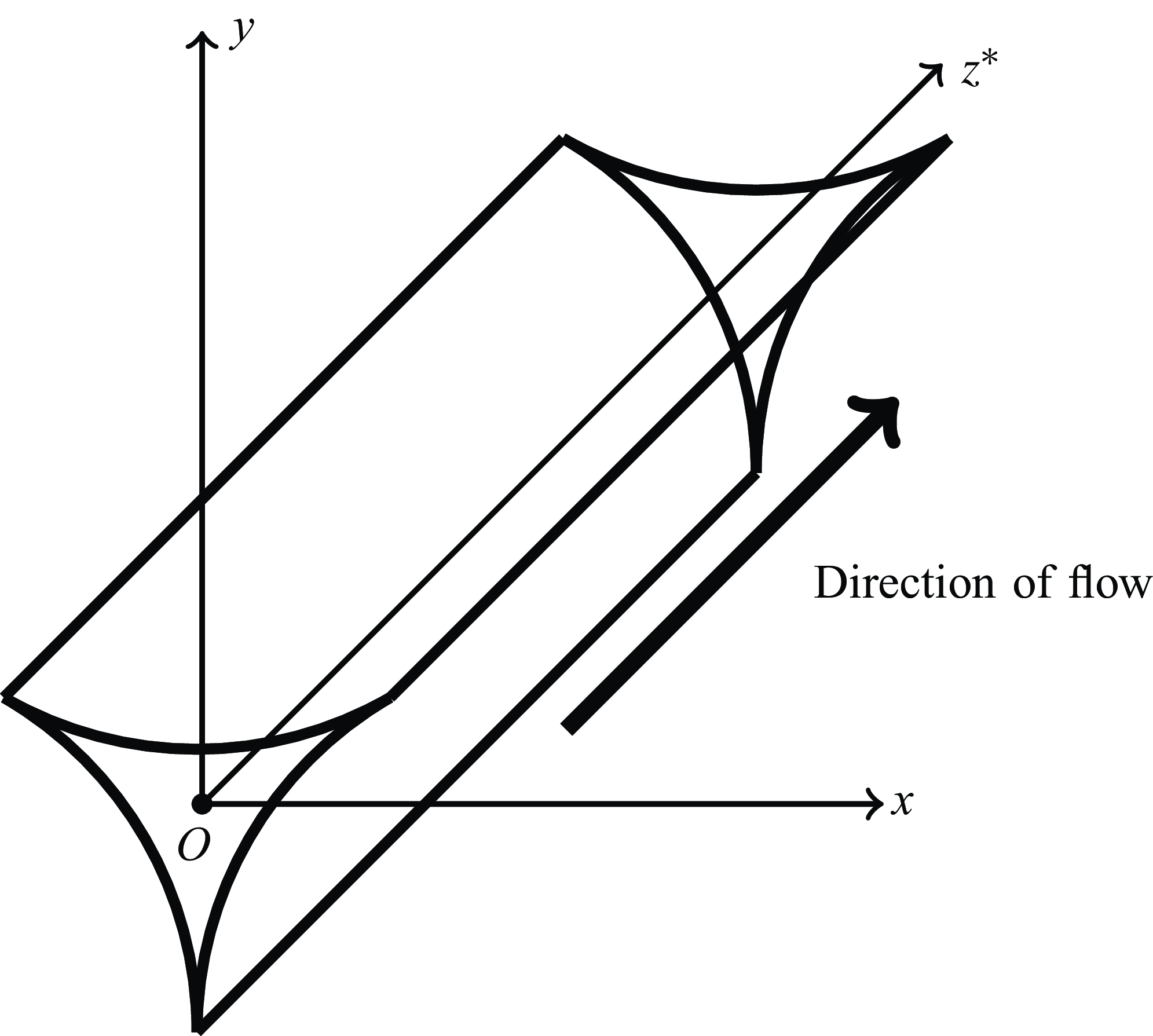


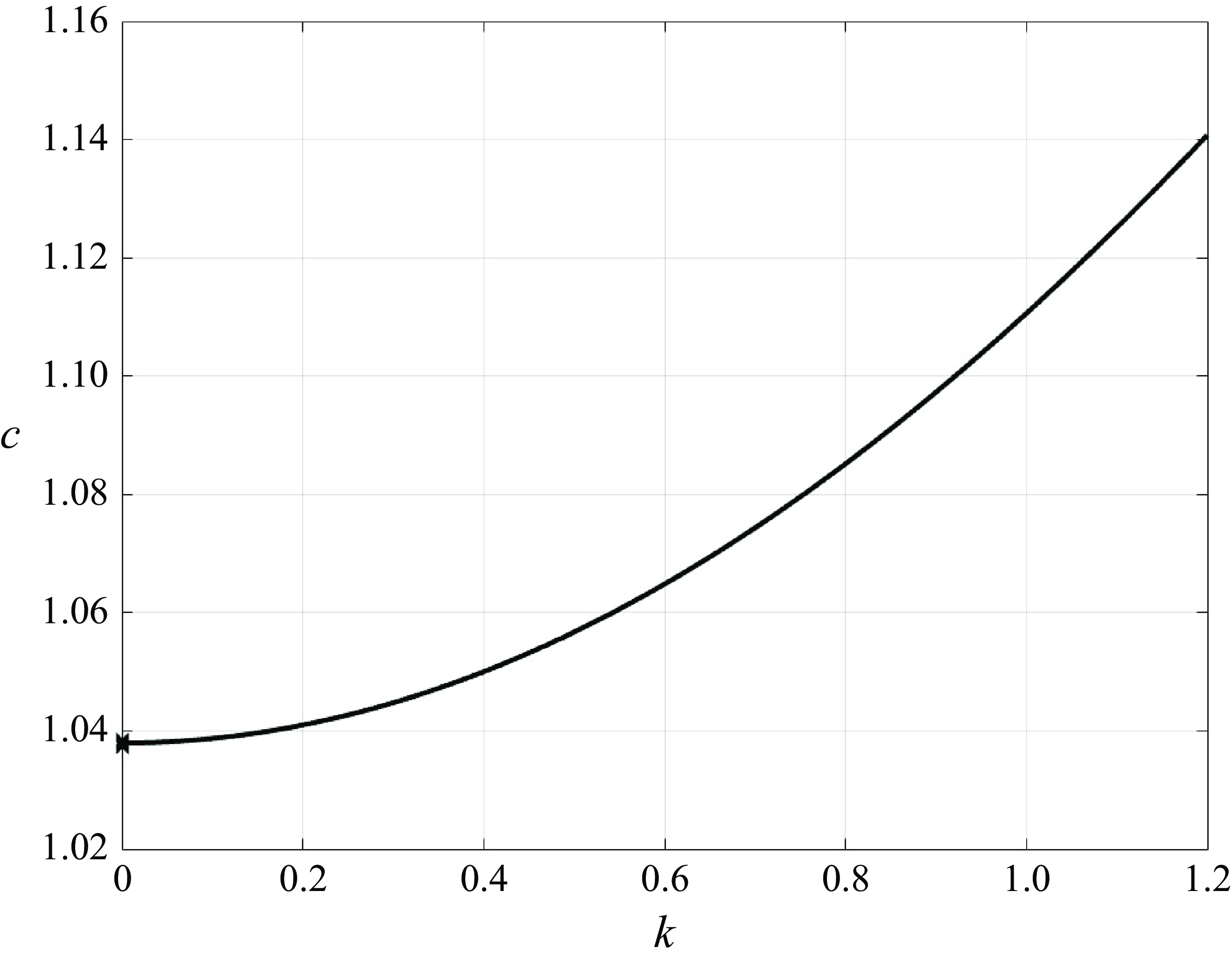


 Open access