


1. Introduction
The propulsion of floating objects due to auto-generated surface-tension gradients, also known as Marangoni surfing, stands as a fascinating phenomenon observed in the world of living organisms while also bearing promising potential for robotic applications. For example, in nature, this mode of locomotion is employed by water-walking insects for speedy movement in emergency situations (Linsenmair & Jander Reference Linsenmair and Jander1963; Andersen Reference Andersen1976; Schildknecht Reference Schildknecht1976; Bush & Hu Reference Bush and Hu2006; Bush, Hu & Prakash Reference Bush, Hu and Prakash2007; Lang, Seifert & Dettner Reference Lang, Seifert and Dettner2012) and by certain bacterial swarms for rapid interfacial migration toward nutrient-rich regions for further colonisation (Harshey Reference Harshey2003; Daniels et al. Reference Daniels2006; Angelini et al. Reference Angelini, Roper, Kolter, Weitz and Brenner2009; Kearns Reference Kearns2010; Fauvart et al. Reference Fauvart, Phillips, Bachaspatimayum, Verstraeten, Fransaer, Michiels and Vermant2012). In the realm of human-made systems, arguably, the most basic form of Marangoni surfing is realised in a camphor/soap boat, where the gradual dissolution of a camphor/soap piece attached to the back of a boat (representative of a floating object) creates a fore–aft surface-tension asymmetry (with associated Marangoni flows) that leads to the self-propulsion of the craft. Over the years, various adaptations of this rudimentary surfer concept have been developed, with sizes ranging from a few micrometres to more than ten centimetres (Kitahata et al. Reference Kitahata, Hiromatsu, Doi, Nakata and Rafiqul Islam2004; Su Reference Su2007; Bassik, Abebe & Gracias Reference Bassik, Abebe and Gracias2008; Soh, Bishop & Grzybowski Reference Soh, Bishop and Grzybowski2008; Shibuya & Matsushita Reference Shibuya and Matsushita2009; Nakata & Murakami Reference Nakata and Murakami2010; Suematsu et al. Reference Suematsu, Nakata, Awazu and Nishimori2010; Soh, Branicki & Grzybowski Reference Soh, Branicki and Grzybowski2011; Jin et al. Reference Jin, Marmur, Ikkala and Ras2012; Li et al. Reference Li, Qiao, Liu and Luo2012; Luo et al. Reference Luo, Li, Qiao and Liu2012; Qiao et al. Reference Qiao, Xiao, Lu and Luo2012; Sharma, Chang & Velev Reference Sharma, Chang and Velev2012; Zhao & Pumera Reference Zhao and Pumera2012; Bansagi et al. Reference Bánsági, Wrobel, Scott and Taylor2013; Renney, Brewer & Mooibroek Reference Renney, Brewer and Mooibroek2013; Zhang et al. Reference Zhang, Duan, Liu and Sen2013; Burton, Cheng & Bush Reference Burton, Cheng and Bush2014; Pimienta & Antoine Reference Pimienta and Antoine2014; Xiao, Jiang & Shi Reference Xiao, Jiang and Shi2014; Maggi et al. Reference Maggi, Saglimbeni, Dipalo, De Angelis and Di Leonardo2015; Ooi et al. Reference Ooi, Van Nguyen, Evans, Gendelman, Bormashenko and Nguyen2015; Satterwhite-Warden et al. Reference Satterwhite-Warden, Kondepudi, Dixon and Rusling2015; Srinivasan et al. Reference Srinivasan, Roche, Ravaine and Kuhn2015; Girot et al. Reference Girot, Danne, Würger, Bickel, Ren, Loudet and Pouligny2016; Liakos et al. Reference Liakos, Salvagnini, Scarpellini, Carzino, Beltran, Mele, Murino and Athanassiou2016; Musin et al. Reference Musin, Grynyov, Frenkel and Bormashenko2016; Srivastava & Schmidt Reference Srivastava and Schmidt2016; Wang et al. Reference Wang, Yuan, Lu, Tan, Liu, Yu, He and Liu2016; Frenkel et al. Reference Frenkel, Multanen, Grynyov, Musin, Bormashenko and Bormashenko2017; Koyano et al. Reference Koyano, Gryciuk, Skrobanska, Malecki, Sumino, Kitahata and Gorecki2017; Sharma et al. Reference Sharma, Corcoran, Garoff, Przybycien and Tilton2017; Zhang et al. Reference Zhang, Yuan, Qiu, Zhang, Chen and Huang2017; Ivanov & Nikolov Reference Ivanov and Nikolov2019; Löffler et al. Reference Löffler, Hanczyc and Gorecki2019; Morohashi, Imai & Toyota Reference Morohashi, Imai and Toyota2019; Sur, Masoud & Rothstein Reference Sur, Masoud and Rothstein2019; Pena-Francesch, Giltinan & Sitti Reference Pena-Francesch, Giltinan and Sitti2019; Dietrich et al. Reference Dietrich, Jaensson, Buttinoni, Volpe and Isa2020; Sur et al. Reference Sur, Uvanovic, Masoud and Rothstein2021). Notably, some of the more recent and sophisticated versions, such as the robots engineered by Kwak & Bae (Reference Kwak and Bae2017), Kwak, Choi & Bae (Reference Kwak, Choi and Bae2020), Kwak et al. (Reference Kwak, Choi, Maeng and Bae2021), Basualdo et al. (Reference Basualdo, Bolopion, Gauthier and Lambert2021), Timm et al. (Reference Timm, Jafari Kang, Rothstein and Masoud2021) and Bechard et al. (Reference Bechard, Timm, Masoud and Rothstein2023), have demonstrated capabilities applicable to a wide range of tasks, including environmental sensing and monitoring, microfluidic manipulation and self-assembly.
In order to drive continued progress in the development of advanced surfing robots powered by the Marangoni effect, it is imperative to establish a comprehensive understanding of Marangoni propulsion across a spectrum of operating conditions. Among the fundamental research conducted on this subject to date (Kitahata et al. Reference Kitahata, Hiromatsu, Doi, Nakata and Rafiqul Islam2004; Nagayama et al. Reference Nagayama, Nakata, Doi and Hayashima2004; Soh et al. Reference Soh, Bishop and Grzybowski2008; Lauga & Davis Reference Lauga and Davis2012; Masoud & Shelley Reference Masoud and Stone2014; Masoud & Stone Reference Masoud and Stone2014; Würger Reference Würger2014; Malgaretti, Popescu & Dietrich Reference Malgaretti, Popescu and Dietrich2016; Vandadi, Jafari Kang & Masoud Reference Vandadi, Jafari Kang and Masoud2017; Domínguez & Popescu Reference Domínguez and Popescu2018; Boniface et al. Reference Boniface, Cottin-Bizonne, Kervil, Ybert and Detcheverry2019; Gidituri, Panchagnula & Pototsky Reference Gidituri, Panchagnula and Pototsky2019; Crowdy Reference Crowdy2020, Reference Crowdy2021; Jafari Kang et al. Reference Jafari Kang, Sur, Rothstein and Masoud2020; Boniface et al. Reference Boniface, Cottin-Bizonne, Detcheverry and Ybert2021; Ender & Kierfeld Reference Ender and Kierfeld2021), the predominant focus of the theoretical efforts has been centred on cases characterised by negligible advective transport of mass (or heat) and momentum, where the Péclet and Reynolds numbers (represented by $\textit{Pe}$
and
$\textit{Pe}$
and $\textit{Re}$
, respectively) approach zero. However, many practical scenarios do not conform to such idealised conditions. Consequently, there is a need for further theoretical insights to inform the design of robots capable of efficiently navigating in these non-ideal regimes.
$\textit{Re}$
, respectively) approach zero. However, many practical scenarios do not conform to such idealised conditions. Consequently, there is a need for further theoretical insights to inform the design of robots capable of efficiently navigating in these non-ideal regimes.
To address the aforementioned demand, we examine the Marangoni-driven motion of a chemically active particle along a flat liquid–gas interface. First, we use the reciprocal theorem to derive a generally valid formula relating the propulsion speed of the active surfer to surface and volume integrals involving, respectively, the concentration and velocity fields around it. We then employ the perturbation theory to evaluate those integrals in the limits of small Péclet and Reynolds numbers and show, to the leading order, how the speed of a purely translating surfer changes as a result of non-zero $\textit{Pe}$
and
$\textit{Pe}$
and $\textit{Re}$
. Motivated by our theoretical findings, next, we consider a representative spherical surfer and study its propulsion behaviour over a broad span of
$\textit{Re}$
. Motivated by our theoretical findings, next, we consider a representative spherical surfer and study its propulsion behaviour over a broad span of $\textit{Pe}$
and
$\textit{Pe}$
and $\textit{Re}$
values (well beyond the validity range of the theory) via detailed numerical simulations. The results of our calculations are presented in the form of performance regime maps that pinpoint optimal surfing scenarios. Below, we present our theoretical derivations (§ 2), followed by the description of our computational approach (§ 3). The outcomes of our investigation are discussed afterward (§ 4), and concluding remarks are given at the end (§ 5).
$\textit{Re}$
values (well beyond the validity range of the theory) via detailed numerical simulations. The results of our calculations are presented in the form of performance regime maps that pinpoint optimal surfing scenarios. Below, we present our theoretical derivations (§ 2), followed by the description of our computational approach (§ 3). The outcomes of our investigation are discussed afterward (§ 4), and concluding remarks are given at the end (§ 5).

Figure 1. Schematic of a half-submerged spherical surfer located atop an (ideally) unbounded liquid layer. The active area of the surfer is coloured red, and the colour map and vector plots represent the concentration distribution and liquid velocity field in the vicinity of the surfer, respectively.
2. Problem statement and perturbation solution
2.1. Assumptions and governing equations
Consider the motion of a particle located at an interface between a semi-infinite layer of gas and an identical layer of liquid with density $\varrho$
, viscosity
$\varrho$
, viscosity $\mu$
and surface tension
$\mu$
and surface tension $\gamma$
. The movement of the particle is caused by an asymmetric release of a chemical species, with diffusivity
$\gamma$
. The movement of the particle is caused by an asymmetric release of a chemical species, with diffusivity $\mathscr{D}$
, from the particle’s surface (see, e.g. figure 1). Our initial goal is to formulate a theoretical expression for the self-propulsion speed of the particle in the limits of small Péclet and Reynolds numbers. To reduce the complexity of the derivation, we assume that (i) the liquid–gas interface is flat, (ii) the effect of flow in the gas phase is negligible, (iii) the released chemical species is soluble in the bulk of the liquid layer, (iv) the liquid is at rest and contains no amount of the chemical species far from the particle, (v) the liquid is Newtonian with constant density and viscosity that are unaffected by the presence of the solute, (vi) the surface tension of the liquid varies linearly with the concentration of the chemical species, (vii) no velocity slip occurs on the wetted surface of the surfer due to tangential concentration gradients and (viii) the particle undergoes a pure translational motion along a straight line parallel to the interface.
$\mathscr{D}$
, from the particle’s surface (see, e.g. figure 1). Our initial goal is to formulate a theoretical expression for the self-propulsion speed of the particle in the limits of small Péclet and Reynolds numbers. To reduce the complexity of the derivation, we assume that (i) the liquid–gas interface is flat, (ii) the effect of flow in the gas phase is negligible, (iii) the released chemical species is soluble in the bulk of the liquid layer, (iv) the liquid is at rest and contains no amount of the chemical species far from the particle, (v) the liquid is Newtonian with constant density and viscosity that are unaffected by the presence of the solute, (vi) the surface tension of the liquid varies linearly with the concentration of the chemical species, (vii) no velocity slip occurs on the wetted surface of the surfer due to tangential concentration gradients and (viii) the particle undergoes a pure translational motion along a straight line parallel to the interface.
Let $\boldsymbol{r} = x \boldsymbol{e\!}_x + y \boldsymbol{e\!}_y + z \boldsymbol{e}_z$
be the position vector with
$\boldsymbol{r} = x \boldsymbol{e\!}_x + y \boldsymbol{e\!}_y + z \boldsymbol{e}_z$
be the position vector with $r = |\boldsymbol{r}|$
in the Cartesian coordinate system
$r = |\boldsymbol{r}|$
in the Cartesian coordinate system $(x,y,z)$
, with the unit vectors
$(x,y,z)$
, with the unit vectors $\boldsymbol{e\!}_x$
,
$\boldsymbol{e\!}_x$
, $\boldsymbol{e\!}_y$
and
$\boldsymbol{e\!}_y$
and $\boldsymbol{e}_z$
such that
$\boldsymbol{e}_z$
such that $\boldsymbol{e\!}_x$
is aligned with the propulsion direction of the surfer,
$\boldsymbol{e\!}_x$
is aligned with the propulsion direction of the surfer, $\boldsymbol{e}_z$
is normal to the interface pointing away from the liquid and the origin of the coordinates coincides with the geometrical centre of the three-phase contact line denoted by
$\boldsymbol{e}_z$
is normal to the interface pointing away from the liquid and the origin of the coordinates coincides with the geometrical centre of the three-phase contact line denoted by $l_{\!p}$
(see figure 1). Also, let
$l_{\!p}$
(see figure 1). Also, let $c$
,
$c$
, $\boldsymbol{u} = u_x \boldsymbol{e\!}_x + u_y \boldsymbol{e\!}_y + u_z \boldsymbol{e}_z$
and
$\boldsymbol{u} = u_x \boldsymbol{e\!}_x + u_y \boldsymbol{e\!}_y + u_z \boldsymbol{e}_z$
and $p$
, represent, respectively, the dimensionless, steady-state concentration field of the chemical species and the velocity and pressure fields of the liquid. With these definitions and the above-mentioned assumptions, the equations that govern the distributions of
$p$
, represent, respectively, the dimensionless, steady-state concentration field of the chemical species and the velocity and pressure fields of the liquid. With these definitions and the above-mentioned assumptions, the equations that govern the distributions of $c$
,
$c$
, $\boldsymbol{u}$
and
$\boldsymbol{u}$
and $p$
in a coordinate system attached to the particle are (see, e.g. Masoud & Stone Reference Masoud and Stone2019, p. 37)
$p$
in a coordinate system attached to the particle are (see, e.g. Masoud & Stone Reference Masoud and Stone2019, p. 37)
 \begin{align} {\nabla} ^{2} c = \textit{Pe} \left ( \boldsymbol{u} - \mathscr{U} \boldsymbol{e\!}_x \right ) \boldsymbol{\cdot }\boldsymbol{\nabla \!} c, \end{align}
with the boundary conditions
 \begin{align} &\boldsymbol{n} \boldsymbol{\cdot }\boldsymbol{\nabla \!} c = 0 \quad \text{ for } \quad \boldsymbol{r} \in S_i, \end{align}
 \begin{align} &c \to 0 \quad \text{as} \quad r \to \infty , \end{align}
and
 \begin{align} &\boldsymbol{\nabla } \boldsymbol{\cdot }\boldsymbol{\sigma } - \textit{Re}\! \left ( \boldsymbol{u} - \mathscr{U} \boldsymbol{e\!}_x \right ) \boldsymbol{\cdot }\boldsymbol{\nabla } \boldsymbol{u} = {\nabla} ^2 \boldsymbol{u} - \boldsymbol{\nabla \!} p - \textit{Re}\! \left ( \boldsymbol{u} - \mathscr{U} \boldsymbol{e\!}_x \right ) \boldsymbol{\cdot }\boldsymbol{\nabla \!} \boldsymbol{u} = \boldsymbol{0}, \end{align}
 \begin{align} &\boldsymbol{\nabla } \boldsymbol{\cdot }\boldsymbol{u} = 0, \end{align}
with the boundary conditions
 \begin{align} &\boldsymbol{u} = \mathscr{U} \boldsymbol{e\!}_x \quad \text{for} \quad \boldsymbol{r} \in S_{\!p}, \end{align}
 \begin{align} &\boldsymbol{u} \to \boldsymbol{0} \quad \text{as} \quad r \to \infty , \end{align}
 \begin{align} &u_z = 0 \quad \text{and} \quad \left ( \boldsymbol{I} - \boldsymbol{n} \boldsymbol{n} \right ) \boldsymbol{\cdot }\left ( \boldsymbol{n} \boldsymbol{\cdot }\boldsymbol{\sigma } \right ) = -\! \left ( \frac {\partial u_x}{\partial z} \boldsymbol{e\!}_x + \frac {\partial u_y}{\partial z} \boldsymbol{e\!}_y \right ) = - \boldsymbol{\nabla }_{\!S_i} \gamma \quad \text{ for } \quad \boldsymbol{r} \in S_i. \end{align}
Here, $S_i$
,
$S_i$
, $S_{\!p}$
,
$S_{\!p}$
, $\boldsymbol{\sigma } = - p \boldsymbol{I} + \mu [ \boldsymbol{\nabla } \boldsymbol{u} + ( \boldsymbol{\nabla } \boldsymbol{u} )^T ]$
,
$\boldsymbol{\sigma } = - p \boldsymbol{I} + \mu [ \boldsymbol{\nabla } \boldsymbol{u} + ( \boldsymbol{\nabla } \boldsymbol{u} )^T ]$
, $\boldsymbol{I}$
,
$\boldsymbol{I}$
, $\boldsymbol{n}$
and
$\boldsymbol{n}$
and $\boldsymbol{\nabla }_{\!S_i}$
denote the liquid–gas interface, the wet surface of the surfer, the stress tensor, the identity tensor, the unit normal vector and the surface gradient operator taking effect along
$\boldsymbol{\nabla }_{\!S_i}$
denote the liquid–gas interface, the wet surface of the surfer, the stress tensor, the identity tensor, the unit normal vector and the surface gradient operator taking effect along $S_i$
, respectively. Also,
$S_i$
, respectively. Also,
 \begin{align} \textit{Pe} = \dfrac {U^\star \ell }{\mathscr{D}}, \qquad \textit{Re} = \dfrac {\varrho U^\star \ell }{\mu } \qquad \text{and} \qquad \mathscr{U} =\,\, \begin{matrix}\underset {\tilde {}}{U}\\[-5pt]\hline {U^\star}\end{matrix}\,\,\,, \end{align}
where $\ell$
is the radius of the smallest sphere that encloses the surfer,
$\ell$
is the radius of the smallest sphere that encloses the surfer, $\underset {\tilde {}}{\boldsymbol{U}} = \underset {\tilde {}}{U} \boldsymbol{e\!}_x$
is the (dimensional) propulsion velocity of the surfer and
$\underset {\tilde {}}{\boldsymbol{U}} = \underset {\tilde {}}{U} \boldsymbol{e\!}_x$
is the (dimensional) propulsion velocity of the surfer and $U^\star$
represents the value of
$U^\star$
represents the value of $\underset {\tilde {}}{U}$
in the absence of advective effects (i.e. when the concentration and flow fields are governed by diffusion and Stokes equations, respectively). Note that we intentionally refrained from specifying a boundary condition for
$\underset {\tilde {}}{U}$
in the absence of advective effects (i.e. when the concentration and flow fields are governed by diffusion and Stokes equations, respectively). Note that we intentionally refrained from specifying a boundary condition for $c$
on
$c$
on $S_{\!p}$
in order to avoid constraining the problem to a particular release mechanism.
$S_{\!p}$
in order to avoid constraining the problem to a particular release mechanism.
2.2. An integral formulation for the propulsion speed
Consider the auxiliary problem of Stokes flow around the same surfer travelling with velocity ${\underset {\tilde {}}{U}}{}_{\!a} = {\underset {\tilde {}}{U}}{}_{\!a} {\boldsymbol{e}}_x$
(where
${\underset {\tilde {}}{U}}{}_{\!a} = {\underset {\tilde {}}{U}}{}_{\!a} {\boldsymbol{e}}_x$
(where ${\underset {\tilde {}}{U}}{}_{\!a} = |{\underset {\tilde {}}{U}}{}_{\!a}|$
) when no surface-tension gradients (i.e. Marangoni stresses) are present. The (dimensionless) velocity and the stress fields, in this case, follow
${\underset {\tilde {}}{U}}{}_{\!a} = |{\underset {\tilde {}}{U}}{}_{\!a}|$
) when no surface-tension gradients (i.e. Marangoni stresses) are present. The (dimensionless) velocity and the stress fields, in this case, follow
 \begin{align} &\boldsymbol{\nabla } \boldsymbol{\cdot }\boldsymbol{\sigma }_{\!a} = {\nabla} ^2 \boldsymbol{u}_a - \boldsymbol{\nabla \!} p_a = \boldsymbol{0}, \end{align}
 \begin{align} &\boldsymbol{\nabla } \boldsymbol{\cdot }\boldsymbol{u}_a = 0, \end{align}
with the boundary conditions
 \begin{align} &\boldsymbol{u}_a = \boldsymbol{e\!}_x \quad \text{for} \quad \boldsymbol{r} \in S_{\!p}, \end{align}
 \begin{align} &\boldsymbol{u}_a \to \boldsymbol{0} \quad \text{as} \quad r \to \infty , \end{align}
 \begin{align} &u_{a,z} = 0 \quad \text{and} \quad \left ( \boldsymbol{I} - \boldsymbol{n} \boldsymbol{n} \right ) \boldsymbol{\cdot }\left ( \boldsymbol{n} \boldsymbol{\cdot }\boldsymbol{\sigma }_{\!a} \right ) = \boldsymbol{0} \quad \text{ for } \quad \boldsymbol{r} \in S_i. \end{align}
According to Lamb’s general solution of the Stokes equations (Lamb Reference Lamb1932, see also Brenner & Cox Reference Brenner and Cox1963), far from the surfer, $\boldsymbol{u}_a$
behaves as
$\boldsymbol{u}_a$
behaves as
 \begin{align} \boldsymbol{u}_a = {_{-1}\boldsymbol{u}}_a + \mathscr{O}(r^{-2}), \end{align}
where
 \begin{align} {_{-1}\boldsymbol{u}}_a &= \frac {1}{4 \pi r}\! \left ( \boldsymbol{I} + \frac {\boldsymbol{r} \boldsymbol{r} }{r^2} \right ) \boldsymbol{\cdot }F_{\!a} \, \boldsymbol{e\!}_x, \end{align}
 \begin{align} - F_{\!a} \boldsymbol{e\!}_x &= \boldsymbol{F}_{\!a} = \int _{S_{\!p}} \boldsymbol{n} \boldsymbol{\cdot }\boldsymbol{\sigma }_{\!a} \; {\textrm {d}S}. \end{align}
Next, apply the reciprocal theorem between the velocity–stress pairs $ ( \boldsymbol{u} , \boldsymbol{\sigma } )$
and
$ ( \boldsymbol{u} , \boldsymbol{\sigma } )$
and $ ( \boldsymbol{u}_a , \boldsymbol{\sigma }_{\!a} )$
(see, e.g. Masoud & Stone Reference Masoud and Stone2019, p. 14) to arrive at
$ ( \boldsymbol{u}_a , \boldsymbol{\sigma }_{\!a} )$
(see, e.g. Masoud & Stone Reference Masoud and Stone2019, p. 14) to arrive at
 \begin{equation} \int _S \boldsymbol{n} \boldsymbol{\cdot }\boldsymbol{\sigma } \boldsymbol{\cdot }\boldsymbol{u}_a \; {\textrm {d}S} - \int _S \boldsymbol{n} \boldsymbol{\cdot }\boldsymbol{\sigma }_{\!a} \boldsymbol{\cdot }\boldsymbol{u} \; {\textrm {d}S} = \textit{Re} \int _V\! \left ( \mathscr{U} \boldsymbol{e\!}_x - \boldsymbol{u} \right ) \boldsymbol{\cdot }\boldsymbol{\nabla } \boldsymbol{u} \boldsymbol{\cdot }\boldsymbol{u}_a \; \textrm {d}V, \end{equation}
where $V$
and
$V$
and $S = S_i + S_{\!p} + S_\infty$
represent the volume and outer surface of the entire liquid domain, respectively. The integrals over
$S = S_i + S_{\!p} + S_\infty$
represent the volume and outer surface of the entire liquid domain, respectively. The integrals over $S_\infty$
(the bounding surfaces at very large distances) are zero since the velocities decay at least as fast as
$S_\infty$
(the bounding surfaces at very large distances) are zero since the velocities decay at least as fast as $1 / r$
. Hence, we have
$1 / r$
. Hence, we have
 \begin{align} & \int _{S_i} \boldsymbol{n} \boldsymbol{\cdot }\boldsymbol{\sigma } \boldsymbol{\cdot }\boldsymbol{u}_a \; {\textrm {d}S} + \int _{S_{\!p}} \boldsymbol{n} \boldsymbol{\cdot }\boldsymbol{\sigma } \boldsymbol{\cdot }\boldsymbol{u}_a \; {\textrm {d}S}- \int _{S_i} \boldsymbol{n} \boldsymbol{\cdot }\boldsymbol{\sigma }_{\!a} \boldsymbol{\cdot }\boldsymbol{u} \; {\textrm {d}S} \notag \\ & -\! \int _{S_{\!p}} \boldsymbol{n} \boldsymbol{\cdot }\boldsymbol{\sigma }_{\!a} \boldsymbol{\cdot }\boldsymbol{u} \; {\textrm {d}S}= \textit{Re} \int _V\! \left ( \mathscr{U} \boldsymbol{e\!}_x - \boldsymbol{u} \right ) \boldsymbol{\cdot }\boldsymbol{\nabla } \boldsymbol{u} \boldsymbol{\cdot }\boldsymbol{u}_a \; \textrm {d}V. \end{align}
From the force balance on the surfer and the boundary conditions described by (2.2c )–(2.2), (2.1b ) and (2.1c ), we infer
 \begin{align} \left ( \boldsymbol{n} \boldsymbol{\cdot }\boldsymbol{\sigma } \boldsymbol{\cdot }\boldsymbol{u}_a \right ) \big |_{S_i} & = - \boldsymbol{\nabla }_{\!S_i}\! \gamma \boldsymbol{\cdot }\boldsymbol{u}_a|_{S_i}, \end{align}
 \begin{align} \int _{S_{\!p}} \boldsymbol{n} \boldsymbol{\cdot }\boldsymbol{\sigma } \boldsymbol{\cdot }\boldsymbol{u}_a \; {\textrm {d}S} & = \int _{S_{\!p}} \boldsymbol{n} \boldsymbol{\cdot }\boldsymbol{\sigma } \; {\textrm {d}S} \boldsymbol{\cdot }\boldsymbol{e\!}_x = -\! \int _{l_{\!p}} \gamma \boldsymbol{t} \; \textrm {d}l \boldsymbol{\cdot }\boldsymbol{e\!}_x = - \boldsymbol{F}_{\!\textit{st}} \boldsymbol{\cdot }\boldsymbol{e\!}_x = - F_{\!\textit{st}}, \end{align}
 \begin{align} \int _{S_i} \boldsymbol{n} \boldsymbol{\cdot }\boldsymbol{\sigma }_{\!a} \boldsymbol{\cdot }\boldsymbol{u} \; {\textrm {d}S}& = 0, \end{align}
 \begin{align} \int _{S_{\!p}} \boldsymbol{n} \boldsymbol{\cdot }\boldsymbol{\sigma }_{\!a} \boldsymbol{\cdot }\boldsymbol{u} \; {\textrm {d}S} & = \int _{S_{\!p}} \boldsymbol{n} \boldsymbol{\cdot }\boldsymbol{\sigma }_{\!a} \; {\textrm {d}S} \boldsymbol{\cdot }\mathscr{U} \boldsymbol{e\!}_x = - F_{\!a} \, \mathscr{U}, \end{align}
where $\boldsymbol{t}$
is the unit vector tangent to
$\boldsymbol{t}$
is the unit vector tangent to $S_i$
and normal to
$S_i$
and normal to $l_{\!p}$
, and
$l_{\!p}$
, and $F_{\!a}$
is non-dimensionalised by
$F_{\!a}$
is non-dimensionalised by $\mu {\underset {\tilde {}}{U}}{}_a \ell$
. Therefore, we can write
$\mu {\underset {\tilde {}}{U}}{}_a \ell$
. Therefore, we can write
 \begin{align} - F_{\!\textit{st}} - \int _{S_i} \boldsymbol{\nabla }_{\!S_i} \gamma \boldsymbol{\cdot }\boldsymbol{u}_a \; {\textrm {d}S} + F_{\!a} \, \mathscr{U} = \textit{Re} \int _V \left ( \mathscr{U} \boldsymbol{e\!}_x - \boldsymbol{u} \right ) \boldsymbol{\cdot }\boldsymbol{\nabla } \boldsymbol{u} \boldsymbol{\cdot }\boldsymbol{u}_a \; \textrm {d}V, \end{align}
which leads to
 \begin{align} \mathscr{U} &= \frac {F_{\!\textit{st}}}{F_{\!a}} + \int _{S_i} \boldsymbol{\nabla }_{\!S_i} \gamma \boldsymbol{\cdot }\Big ( \frac {\boldsymbol{u}_a}{F_{\!a}} \Big ) \; {\textrm {d}S} + \textit{Re} \int _V \left ( \mathscr{U} \boldsymbol{e\!}_x - \boldsymbol{u} \right ) \boldsymbol{\cdot }\boldsymbol{\nabla } \boldsymbol{u} \boldsymbol{\cdot }\Big ( \frac {\boldsymbol{u}_a}{F_{\!a}} \Big ) \; \textrm {d}V. \end{align}
The above integral relation for the propulsion speed can be expressed alternatively as
 \begin{align} \mathscr{U} &= -\! \int _{S_i}\! \left ( \gamma - \gamma _0 \right ) \boldsymbol{\nabla }_{\!S_i} \boldsymbol{\cdot }\Big ( \frac {\boldsymbol{u}_a}{F_{\!a}} \Big ) \; {\textrm {d}S} \notag \\ &\quad+ \textit{Re}\! \left [ \int _V \boldsymbol{u} \boldsymbol{\cdot }\boldsymbol{\nabla } \Big ( \frac {\boldsymbol{u}_a}{F_{\!a}} \Big ) \boldsymbol{\cdot }\boldsymbol{u} \; \textrm {d}V - \mathscr{U} \boldsymbol{e\!}_x \boldsymbol{\cdot }\int _V \boldsymbol{\nabla } \Big ( \frac {\boldsymbol{u}_a}{F_{\!a}} \Big ) \boldsymbol{\cdot }\boldsymbol{u} \; \textrm {d}V \right ]\!, \end{align}
given that
 \begin{align} \left ( \mathscr{U} \boldsymbol{e\!}_x - \boldsymbol{u} \right ) \boldsymbol{\cdot }\boldsymbol{\nabla } \boldsymbol{u} \boldsymbol{\cdot }\boldsymbol{u}_a &= \mathscr{U} \boldsymbol{e\!}_x \boldsymbol{\cdot }\boldsymbol{\nabla } \boldsymbol{u} \boldsymbol{\cdot }\boldsymbol{u}_a - \boldsymbol{u} \boldsymbol{\cdot }\boldsymbol{\nabla } \boldsymbol{u} \boldsymbol{\cdot }\boldsymbol{u}_a \notag \\ &= \mathscr{U} \boldsymbol{e\!}_x \boldsymbol{\cdot }\left [ \boldsymbol{\nabla } \left ( \boldsymbol{u} \boldsymbol{\cdot }\boldsymbol{u}_a \right ) - \boldsymbol{\nabla } \boldsymbol{u}_a \boldsymbol{\cdot }\boldsymbol{u} \right ] - \boldsymbol{\nabla } \boldsymbol{\cdot }\left ( \boldsymbol{u} \boldsymbol{u} \boldsymbol{\cdot }\boldsymbol{u}_a \right ) + \boldsymbol{u} \boldsymbol{\cdot }\boldsymbol{\nabla } \boldsymbol{u}_a \boldsymbol{\cdot }\boldsymbol{u} ,\end{align}
and that
 \begin{align} \boldsymbol{\nabla }_{\!S_i} \gamma \boldsymbol{\cdot }\boldsymbol{u}_a = \boldsymbol{\nabla }_{\!S_i} \boldsymbol{\cdot }\left ( \gamma \boldsymbol{u}_a \right ) - \gamma \, \boldsymbol{\nabla }_{\!S_i} \boldsymbol{\cdot }\boldsymbol{u}_a = \boldsymbol{\nabla }_{\!S_i} \boldsymbol{\cdot } [ ( \gamma - \gamma _0 ) \boldsymbol{u}_a ] - \left ( \gamma - \gamma _0 \right ) \boldsymbol{\nabla }_{\!S_i} \boldsymbol{\cdot }\boldsymbol{u}_a. \end{align}
2.3. Singular perturbation expansions of the velocity and concentration fields
Suppose $\textit{Pe} \ll 1$
and
$\textit{Pe} \ll 1$
and $\textit{Re} \ll 1$
, and let
$\textit{Re} \ll 1$
, and let
 \begin{align} \gamma = \gamma _0 - \dfrac {\alpha \dot {m}^\star }{2 \pi \, \mathscr{D} \mu U^\star \, \ell } \, c, \end{align}
where $\gamma _0$
is a non-dimensional constant and
$\gamma _0$
is a non-dimensional constant and $\dot {m}^\star$
is the release rate of the chemical species when the concentration field is governed solely by diffusion. Here,
$\dot {m}^\star$
is the release rate of the chemical species when the concentration field is governed solely by diffusion. Here, $\gamma$
and
$\gamma$
and $c$
are made dimensionless by
$c$
are made dimensionless by $\mu U^\star$
and
$\mu U^\star$
and $\dot {m}^\star / 2 \pi \mathscr{D} \ell$
, respectively. To evaluate (2.10c
) in the limits of small Péclet and Reynolds numbers, we proceed with perturbation expansions of
$\dot {m}^\star / 2 \pi \mathscr{D} \ell$
, respectively. To evaluate (2.10c
) in the limits of small Péclet and Reynolds numbers, we proceed with perturbation expansions of $c$
and
$c$
and $\boldsymbol{u}$
in terms of
$\boldsymbol{u}$
in terms of $\textit{Pe}$
and
$\textit{Pe}$
and $\textit{Re}$
. It is widely known that regular expansions fail to deliver satisfactory approximations due to the far-field behaviour of the concentration and velocity distributions in the purely diffusive and purely viscous limits. Therefore, we adopt the singular perturbation technique, which involves distinct expansions for regions in proximity to and distant from the particle, referred to as the inner and outer regions, respectively (see, e.g. Lagerstrom & Cole Reference Lagerstrom and Cole1955; Kaplun Reference Kaplun1957; Kaplun & Lagerstrom Reference Kaplun and Lagerstrom1957; Proudman & Pearson Reference Proudman and Pearson1957; Van Dyke Reference Van Dyke1964; Hinch Reference Hinch1991; Leal Reference Leal2007). The inner and outer expansions are asymptotically matched in an intermediate region, where both of them are applicable. As demonstrated by Lovalenti & Brady (Reference Lovalenti and Brady1993), these regional expansions can be merged (while carefully avoiding duplication of overlapping regions) to form approximations that remain uniformly valid across the domain
$\textit{Re}$
. It is widely known that regular expansions fail to deliver satisfactory approximations due to the far-field behaviour of the concentration and velocity distributions in the purely diffusive and purely viscous limits. Therefore, we adopt the singular perturbation technique, which involves distinct expansions for regions in proximity to and distant from the particle, referred to as the inner and outer regions, respectively (see, e.g. Lagerstrom & Cole Reference Lagerstrom and Cole1955; Kaplun Reference Kaplun1957; Kaplun & Lagerstrom Reference Kaplun and Lagerstrom1957; Proudman & Pearson Reference Proudman and Pearson1957; Van Dyke Reference Van Dyke1964; Hinch Reference Hinch1991; Leal Reference Leal2007). The inner and outer expansions are asymptotically matched in an intermediate region, where both of them are applicable. As demonstrated by Lovalenti & Brady (Reference Lovalenti and Brady1993), these regional expansions can be merged (while carefully avoiding duplication of overlapping regions) to form approximations that remain uniformly valid across the domain $V$
(see also Dehdashti & Masoud Reference Dehdashti and Masoud2020). Following this approach,
$V$
(see also Dehdashti & Masoud Reference Dehdashti and Masoud2020). Following this approach, $c$
and
$c$
and $\boldsymbol{u}$
can be expressed as
$\boldsymbol{u}$
can be expressed as
 \begin{align} c &= \underbrace {c^{(0,0)}}_{\substack {\text{zeroth-order}\\\text{solution}}} + \underbrace {\textit{Pe} \, c^{(1,0)} }_{\substack {\text{First-order inner}\\\text{approximation}}} + \underbrace {\textit{Pe} \, \check {c}^{(1,0)}}_{\substack {\text{First-order outer}\\\text{approximation}}} - \underbrace {\left ( c^{(0,0)}_\infty + \textit{Pe} \, c^{(1,0)}_\infty \right )}_{\text{Overlapping terms}} \notag \\ &\quad+ \mathscr{O}\big(\textit{Pe}^2 \ln \textit{Pe}\big) + \mathscr{O}(\textit{Pe} \, \textit{Re} \ln \textit{Re}), \end{align}
 \begin{align} \boldsymbol{u} &= \underbrace {\boldsymbol{u}^{(0,0)}}_{\substack {\text{zeroth-order}\\\text{solution}}} + \underbrace { \textit{Re} \ln \textit{Re} \, \boldsymbol{u}^{(0,1)} + \textit{Re} \, \boldsymbol{u}^{(0,2)}}_{\substack {\text{First- and second-order}\\\text{inner approximations}}} + \underbrace {\textit{Re} \, {\tilde {\boldsymbol{u}}}^{(0,1)}}_{\substack {\text{First-order outer}\\\text{approximation}}} \notag \\ &\quad- \underbrace {\left ( \boldsymbol{u}^{(0,0)}_\infty + \textit{Re} \ln \textit{Re} \, \boldsymbol{u}^{(0,1)}_\infty + \textit{Re} \, \boldsymbol{u}^{(0,2)}_\infty \right )}_{\text{Overlapping terms}} + \, \mathscr{O}\big(\textit{Re}^2 \ln \textit{Re}\big) + \mathscr{O}(\textit{Pe} \ln \textit{Pe}), \end{align}
where the infinity subscript denotes the leading-order contributions to the corresponding terms in the limit that $r \to \infty$
. Also,
$r \to \infty$
. Also, $\vee$
and
$\vee$
and $\sim$
overbars denote that the concentration and velocity fields, as well as the
$\sim$
overbars denote that the concentration and velocity fields, as well as the $\boldsymbol{\nabla }$
and
$\boldsymbol{\nabla }$
and ${\nabla} ^2$
operators in the following equations, are written in terms of the stretched (rescaled) position vectors
${\nabla} ^2$
operators in the following equations, are written in terms of the stretched (rescaled) position vectors $\check {\boldsymbol{r}} = \textit{Pe} \, \boldsymbol{r}$
and
$\check {\boldsymbol{r}} = \textit{Pe} \, \boldsymbol{r}$
and $\tilde {\boldsymbol{r}} = \textit{Re} \, \boldsymbol{r}$
, respectively. Note that the coefficients of the expansion terms in (2.14) and (2.15) are not strictly required to be simple powers of the perturbation parameters (i.e.
$\tilde {\boldsymbol{r}} = \textit{Re} \, \boldsymbol{r}$
, respectively. Note that the coefficients of the expansion terms in (2.14) and (2.15) are not strictly required to be simple powers of the perturbation parameters (i.e. $\textit{Re}$
and
$\textit{Re}$
and $\textit{Pe}$
). Instead, they are determined by the boundary and matching conditions, as will become evident shortly.
$\textit{Pe}$
). Instead, they are determined by the boundary and matching conditions, as will become evident shortly.
2.3.1. Zeroth- and first-order approximations for the concentration field
Substituting the zeroth-order term along with the inner and outer expansions from (2.14) into (2.1) and equating like powers of $\textit{Pe}$
, we arrive at the following boundary value problems:
$\textit{Pe}$
, we arrive at the following boundary value problems:
 \begin{align} &{\nabla} ^2 c^{(0,0)} = 0, \end{align}
 \begin{align} &\boldsymbol{n} \boldsymbol{\cdot }\boldsymbol{\nabla \!} c^{(0,0)} = 0 \quad \text{for} \quad \boldsymbol{r} \in S_i, \end{align}
 \begin{align} & c^{(0,0)} \to 0 \quad \text{as} \quad r \to \infty , \end{align}
 \begin{align} & \check {\boldsymbol{\nabla} }^2 \check {c}^{(1,0)} = - \boldsymbol{e\!}_x \boldsymbol{\cdot }\check {\boldsymbol{\nabla }} \check {c}^{(1,0)}, \end{align}
 \begin{align} &\boldsymbol{n} \boldsymbol{\cdot }\check {\boldsymbol{\nabla }} \check {c}^{(1,0)} = 0 \quad \text{for} \quad \check {\boldsymbol{r}} \in S_i, \end{align}
 \begin{align} & \check {c}^{(1,0)} \to 0 \quad \text{as} \quad \check {r} \to \infty , \end{align}
 \begin{align} & {\nabla} ^2 c^{(1,0)} = \big ( \boldsymbol{u}^{(0,0)} - \boldsymbol{e\!}_x \big ) \boldsymbol{\cdot }\boldsymbol{\nabla \!} c^{(0,0)}, \end{align}
 \begin{align} & \boldsymbol{n} \boldsymbol{\cdot }\boldsymbol{\nabla \!} c^{(1,0)} = 0 \quad \text{ for } \quad \boldsymbol{r} \in S_i, \end{align}
 \begin{align} & \lim _{r \to \infty } c^{(0,0)} + \textit{Pe} \lim _{r \to \infty } c^{(1,0)} = \textit{Pe} \lim _{\check {r} \to 0} \, \check {c}^{(1,0)}. \end{align}
Following Brenner (Reference Brenner1963), the asymptotic solutions to (2.15)–(2.17) in the limits of $r \gg 1$
and
$r \gg 1$
and $\check {r} \ll 1$
are given by
$\check {r} \ll 1$
are given by
 \begin{align} c^{(0,0)} &= \frac {1}{r}+ \mathscr{O}(r^{-2}), \end{align}
 \begin{align} c^{(1,0)} &= - \frac {1}{2} \left ( 1 + \frac {x}{r} \right ) + \mathscr{O}(r^{-1}), \end{align}
 \begin{align} \check {c}^{(1,0)} &= \frac {1}{\check {r}} \exp\! \left [ -\frac {1}{2} \left ( \check {r} + \check {x} \right ) \right ] = \frac {1}{\check {r}} - \frac {1}{2} \left ( 1 + \frac {\check {x}}{\check {r}} \right ) + \mathscr{O}(\check {r}). \end{align}
A key parameter for assessing the propulsion efficiency of the surfer (defined either as the distance travelled per unit mass of ‘fuel’ released or as the speed achieved per unit rate of fuel consumed) is the total release rate of the chemical species, expressed as
 \begin{align} \dot {m} = - \mathscr{D} \int _{\textit{S}_{p}} \boldsymbol{n} \boldsymbol{\cdot }\underset {\tilde {}}{\boldsymbol{\nabla }} \underset {\tilde {}}{c} \; \textrm {d}\tilde {S}, \end{align}
where a tilde underbar indicates dimensional variables and operators. Adopting an approach akin to that of Brenner (Reference Brenner1963) (see also Dehdashti & Masoud Reference Dehdashti and Masoud2020), it can be shown that the Sherwood number (denoted by $\textit{Sh}$
), takes the form
$\textit{Sh}$
), takes the form
 \begin{align} \textit{Sh} = \textit{Sh}^\star + \frac {( \textit{Sh}^\star)^2}{2} \textit{Pe} + \mathscr{O} \big(\textit{Pe}^2 \ln \textit{Pe}\big) + \mathscr{O}(\textit{Pe} \, \textit{Re} \ln \textit{Re}), \end{align}
with
 \begin{align} \textit{Sh} = \dfrac {\dot {m}}{2 \pi \mathscr{D}\ell {\underset{\tilde{}}{c}}{}_s} \quad \text{and} \quad \textit{Sh}^\star = \dfrac {\dot {m}^\star }{2 \pi \mathscr{D} \ell {\underset{\tilde{}}{c}}{}_s}, \end{align}
valid for the special case where the wet surface of the surfer is divided into an active region, $S_{\!p}^{a}$
, maintained at a uniform (dimensional) concentration
$S_{\!p}^{a}$
, maintained at a uniform (dimensional) concentration ${\underset{\tilde{}}{c}}{}_s$
, and an inactive region,
${\underset{\tilde{}}{c}}{}_s$
, and an inactive region, $S_{\!p}^{ia}$
, on which a no-flux condition (
$S_{\!p}^{ia}$
, on which a no-flux condition ( $\boldsymbol{n} \boldsymbol{\cdot }\boldsymbol{\nabla \!} c = 0$
) is imposed (see, e.g. Masoud & Rothstein Reference Masoud and Rothstein2022).
$\boldsymbol{n} \boldsymbol{\cdot }\boldsymbol{\nabla \!} c = 0$
) is imposed (see, e.g. Masoud & Rothstein Reference Masoud and Rothstein2022).
2.3.2. Zeroth- and first-order outer approximations for the velocity field
Similarly, substituting the expansion (2.15) into the Navier–Stokes equations (2.2) and collecting terms of equal powers in $\textit{Re}$
yield the following governing equations for the leading-order inner and outer velocity fields:
$\textit{Re}$
yield the following governing equations for the leading-order inner and outer velocity fields:
 \begin{align} &\boldsymbol{\nabla } \boldsymbol{\cdot }\boldsymbol{\sigma }^{(0,0)} = {\nabla} ^2 \boldsymbol{u}^{(0,0)} - \boldsymbol{\nabla \!} p^{(0,0)} = \boldsymbol{0}, \end{align}
 \begin{align} &\boldsymbol{\nabla } \boldsymbol{\cdot }\boldsymbol{u}^{(0,0)} = 0, \end{align}
 \begin{align} &\boldsymbol{u}^{(0,0)} = \boldsymbol{e\!}_x \quad \text{for} \quad \boldsymbol{r} \in S_{\!p}, \end{align}
 \begin{align} &\boldsymbol{u}^{(0,0)} \to \boldsymbol{0} \quad \text{as} \quad r \to \infty , \end{align}
 \begin{align} &u^{(0,0)}_z = 0 \quad \text{and} \quad \left ( \frac {\partial u^{(0,0)}_x}{\partial z} \boldsymbol{e\!}_x + \frac {\partial u^{(0,0)}_y}{\partial z} \boldsymbol{e\!}_y \right ) = \boldsymbol{\nabla }_{\!S_i} \gamma ^{(0,0)} \quad \text{ for } \quad \boldsymbol{r} \in S_i, \end{align}
 \begin{align} &{\tilde {{\nabla }}}^2 {\tilde {\boldsymbol{u}}}^{(0,1)} - \tilde {\boldsymbol{\nabla }}\! \tilde {p}^{(0,1)} + \boldsymbol{e\!}_x \boldsymbol{\cdot }\tilde {\boldsymbol{\nabla }} {\tilde {\boldsymbol{u}}}^{(0,1)} = \boldsymbol{0}, \end{align}
 \begin{align} &\tilde {\boldsymbol{\nabla }} \boldsymbol{\cdot }{\tilde {\boldsymbol{u}}}^{(0,1)} = 0, \end{align}
 \begin{align} &{\tilde {\boldsymbol{u}}}^{(0,1)} \to {\tilde {\boldsymbol{u}}}^{(0,0)} \quad \text{as} \quad \tilde {r} \to 0, \end{align}
 \begin{align} &{\tilde {\boldsymbol{u}}}^{(0,1)} \to \boldsymbol{0} \quad \text{as} \quad \tilde {r} \to \infty , \end{align}
 \begin{align} &\tilde {u}^{(0,1)}_z = 0 \quad \text{and} \quad \left ( \frac {\partial \tilde {u}^{(0,1)}_x}{\partial \tilde {z}} \boldsymbol{e\!}_x + \frac {\partial \tilde {u}^{(0,1)}_y}{\partial \tilde {z}} \boldsymbol{e\!}_y \right ) = \tilde {\boldsymbol{\nabla }}_{\!S_i} \tilde {\gamma }_\infty ^{(0,0)} \quad \text{ for } \quad \tilde {\boldsymbol{r}} \in S_i. \end{align}
Note that the boundary condition at the interface in (2.26) also ensures that
 \begin{align} \lim _{r \to \infty } \boldsymbol{u}^{(0,0)} = \textit{Re} \lim _{\tilde {r} \to 0} \boldsymbol{u}^{(0,1)}. \end{align}
Let $_{-1} \boldsymbol{u}^{(0,0)}$
be the solution to (2.25) correct to
$_{-1} \boldsymbol{u}^{(0,0)}$
be the solution to (2.25) correct to $\mathscr{O}(r^{-1})$
. This velocity field corresponds to the monopolar contribution of the zeroth-order concentration field, denoted henceforth by
$\mathscr{O}(r^{-1})$
. This velocity field corresponds to the monopolar contribution of the zeroth-order concentration field, denoted henceforth by $_{-1} c^{(0,0)} = 1 / r$
(see (2.19)). As described below,
$_{-1} c^{(0,0)} = 1 / r$
(see (2.19)). As described below, ${_{-1} \boldsymbol{u}}^{(0,0)}$
can be calculated by applying the Fourier transform in the
${_{-1} \boldsymbol{u}}^{(0,0)}$
can be calculated by applying the Fourier transform in the $x$
–
$x$
– $y$
plane.
$y$
plane.
We begin by taking the Fourier transform of $_{-1} c^{(0,0)}$
:
$_{-1} c^{(0,0)}$
:
 \begin{align} \mathfrak{F}_{\textit{xy}} \big \{ _{-1} c^{(0,0)}\big \} = _{-1} {\widehat {c}} ^{(0,0)} &= \int _{-\infty }^\infty \int _{-\infty }^\infty \frac {\exp \big [- i \big ( k_x x + k_y y \big ) \big ]}{\sqrt {x^2 + y^2 + z^2}} \; \textrm {d}x \, \textrm {d}y \notag \\[5pt] &= 2 \pi \int _0^\infty \frac {J_0(k \rho )}{\sqrt {\rho ^2 + z^2}} \, \rho \; \textrm {d}\rho = 2 \pi \frac {\exp ( k z )}{k}, \end{align}
where $i^2 = -1$
,
$i^2 = -1$
, $k = |\boldsymbol{k}|$
with
$k = |\boldsymbol{k}|$
with $\boldsymbol{k} = ( k_x, k_y )$
being the in-plane wave vector,
$\boldsymbol{k} = ( k_x, k_y )$
being the in-plane wave vector, $J_0$
the zeroth-order Bessel function of the first kind and
$J_0$
the zeroth-order Bessel function of the first kind and $\rho = \sqrt {x^2 + y^2}$
(see Gradshteyn & Ryzhik Reference Gradshteyn and Ryzhik2007; Baddour Reference Baddour2011, 6.565-2). Note that
$\rho = \sqrt {x^2 + y^2}$
(see Gradshteyn & Ryzhik Reference Gradshteyn and Ryzhik2007; Baddour Reference Baddour2011, 6.565-2). Note that $z \lt 0$
in the liquid phase beneath the interface, as illustrated in figure 1. Combining the result from (2.28) with the derivation presented in the supplementary material of Masoud & Shelley (Reference Masoud and Shelley2014) for Marangoni-driven Stokes flow, we obtain
$z \lt 0$
in the liquid phase beneath the interface, as illustrated in figure 1. Combining the result from (2.28) with the derivation presented in the supplementary material of Masoud & Shelley (Reference Masoud and Shelley2014) for Marangoni-driven Stokes flow, we obtain
 \begin{align} \mathfrak{F}_{\textit{xy}}\! \! \left \{ _{-1}\boldsymbol{u}^{(0,0)} \right \} = {_{-1}{\widehat {\boldsymbol{u}}}}^{(0,0)} = -\! \left ( \frac {\alpha \dot {m}^\star }{\mathscr{D} \mu U^\star \ell } \right ) \frac {\exp ( k z )}{2} \left [ \frac {i \boldsymbol{k}}{k^2} \left ( 1 + k z \right ) + z \, \boldsymbol{e}_z \right ]\!. \end{align}
Taking the inverse Fourier transform of (2.29), we then find (see again, Gradshteyn & Ryzhik Reference Gradshteyn and Ryzhik2007; Baddour Reference Baddour2011, 6.611-1,6.621-4)
 \begin{align} &{_{-1}\boldsymbol{u}}^{(0,0)} \left ( \frac {\alpha \dot {m}^\star }{4 \pi \mathscr{D} \mu U^\star \ell } \right )^{-1} = - 2 \pi \, \mathfrak{F}^{-1}_{\textit{xy}} \! \! \left \{ \exp ( k z ) \left [ \frac {i \boldsymbol{k}}{k^2} \left ( 1 + k z \right ) + z \, \boldsymbol{e}_z \right ] \right \} \notag \\[5pt] &\,= - 2 \pi \, \boldsymbol{\nabla }_{\!xy} \, \mathfrak{F}^{-1}_{\textit{xy}} \! \! \left \{ \exp ( k z ) \left ( \frac {1 + k z}{k^2} \right ) \right \} - 2 \pi \, \mathfrak{F}^{-1}_{\textit{xy}} \! \! \left \{ \exp ( k z ) z \right \} \boldsymbol{e}_z \notag \\[5pt] &\,= - \boldsymbol{\nabla }_{\!xy} \int _0^\infty \frac {\exp ( k z ) \left ( 1 + k z \right ) }{k^2} J_0 ( k \rho ) \, k \; \textrm {d}k - z \int _0^\infty \exp ( k z ) \, J_0 ( k \rho ) \, k \; \textrm {d}k \, \boldsymbol{e}_z \notag \\[5pt] &\,= - \int _0^\infty \frac {\exp ( k z ) \left ( 1 + k z \right ) }{k^2} \boldsymbol{\nabla }_{\!xy} J_0 ( k \rho ) \, k \; \textrm {d}k + \frac {z^2}{r^3} \, \boldsymbol{e}_z \notag \\[5pt] &\,= \int _0^\infty \exp ( k z ) \left ( 1 + k z \right ) J_1 ( k \rho )\; \textrm {d}k \, \boldsymbol{e\!}_\rho + \frac {z^2}{r^3} \boldsymbol{e}_z \notag \\[5pt] &\,= \left [ \frac {1}{\rho } \left ( 1 + \frac {z}{r} \right ) + \frac {\rho z}{r^3} \right ] \boldsymbol{e\!}_\rho + \frac {z^2}{r^3} \, \boldsymbol{e}_z = \frac {1}{r} \left [ \left ( 1 + 2 \cos \theta \right ) \boldsymbol{e}_r + \frac {\sin \theta \cos \theta }{ 1 - \cos \theta } \boldsymbol{e}_\theta \right ]\!, \end{align}
where
 \begin{align} \boldsymbol{\nabla }_{\textit{xy}} J_0 ( k \rho ) &= \frac {\partial J_0 ( k \rho )}{\partial x} \boldsymbol{e\!}_x + \frac {\partial J_0 ( k \rho )}{\partial y} \boldsymbol{e\!}_y = \frac {{\rm d} J_0 ( k \rho )}{{\rm d} \rho } \boldsymbol{e\!}_\rho = - k J_1 ( k \rho ) \, \boldsymbol{e\!}_\rho , \end{align}
and $J_1$
is the first-order Bessel function of the first kind. Here, we have expressed the velocity field in both cylindrical and spherical coordinate systems,
$J_1$
is the first-order Bessel function of the first kind. Here, we have expressed the velocity field in both cylindrical and spherical coordinate systems, $(\rho , \varphi , z)$
and
$(\rho , \varphi , z)$
and $(r , \theta , \varphi )$
, respectively. The associated unit vectors
$(r , \theta , \varphi )$
, respectively. The associated unit vectors $(\boldsymbol{e\!}_\rho , \boldsymbol{e}_\varphi , \boldsymbol{e}_z)$
and
$(\boldsymbol{e\!}_\rho , \boldsymbol{e}_\varphi , \boldsymbol{e}_z)$
and $(\boldsymbol{e}_r, \boldsymbol{e}_\theta , \boldsymbol{e}_\varphi )$
are related to the Cartesian basis via
$(\boldsymbol{e}_r, \boldsymbol{e}_\theta , \boldsymbol{e}_\varphi )$
are related to the Cartesian basis via
 \begin{align} \boldsymbol{e\!}_\rho &= \cos \varphi \, \boldsymbol{e\!}_x + \sin \varphi \, \boldsymbol{e\!}_y, \end{align}
 \begin{align} \boldsymbol{e}_\varphi &= - \sin \varphi \, \boldsymbol{e\!}_x + \cos \varphi \, \boldsymbol{e\!}_y, \end{align}
 \begin{align} \boldsymbol{e}_z &= \boldsymbol{e}_z, \end{align}
 \begin{align} \boldsymbol{e}_r &= \sin \theta \cos \varphi \, \boldsymbol{e\!}_x + \sin \theta \sin \varphi \, \boldsymbol{e\!}_y + \cos \theta \, \boldsymbol{e}_z, \end{align}
 \begin{align} \boldsymbol{e}_\theta &= \cos \theta \cos \varphi \, \boldsymbol{e\!}_x + \cos \theta \sin \varphi \, \boldsymbol{e\!}_y - \sin \theta \, \boldsymbol{e}_z. \end{align}
Hence, the zeroth-order velocity field admits the following asymptotic representation:
 \begin{align} \boldsymbol{u}^{(0,0)} = \left ( \frac {\alpha \dot {m}^\star }{4 \pi \mathscr{D} \mu U^\star \ell } \right ) \left \{ \frac {1}{r} \left [ \left ( 1 + 2 \cos \theta \right ) \boldsymbol{e}_r + \frac {\sin \theta \cos \theta }{ 1 - \cos \theta } \boldsymbol{e}_\theta \right ]\right \} + \mathscr{O}(r^{-2}), \end{align}
which agrees with the expression reported by Würger (Reference Würger2014).
Next, we seek the solution of (2.24) for ${\tilde {\boldsymbol{u}}}^{(0,1)}$
. As will become clear shortly, it is advantageous to again work in the Fourier space. Hence, following Masoud & Shelley (Reference Masoud and Shelley2014), we rewrite the governing equations as
${\tilde {\boldsymbol{u}}}^{(0,1)}$
. As will become clear shortly, it is advantageous to again work in the Fourier space. Hence, following Masoud & Shelley (Reference Masoud and Shelley2014), we rewrite the governing equations as
 \begin{align} \left ( \frac {\partial ^2 }{\partial \tilde {z}^2} - \tilde {k}^{2} + \boldsymbol{e\!}_x \boldsymbol{\cdot }i \tilde {\boldsymbol{k}} \right ) \big ( \widehat {\tilde {u}}^{(0,1)}_x \boldsymbol{e\!}_x + \widehat {\tilde {u}}^{(0,1)}_y \boldsymbol{e\!}_y \big ) &= i \tilde {\boldsymbol{k}} \widehat {\tilde {p}}^{(0,1)}, \end{align}
 \begin{align} \left ( \frac {\partial ^2 }{\partial \tilde {z}^2} - \tilde {k}^{2} + \boldsymbol{e\!}_x \boldsymbol{\cdot }i \tilde {\boldsymbol{k}} \right ) \widehat {\tilde {u}}^{(0,1)}_z &= \frac {\partial \widehat {\tilde {p}}^{(0,1)}}{\partial \tilde {z}}, \end{align}
 \begin{align} i \tilde {\boldsymbol{k}} \boldsymbol{\cdot }\big ( \widehat {\tilde {u}}^{(0,1)}_x \boldsymbol{e\!}_x + \widehat {\tilde {u}}^{(0,1)}_y \boldsymbol{e\!}_y \big ) + \frac {\partial \widehat {\tilde {u}}^{(0,1)}_z}{\partial \tilde {z}} &= 0, \end{align}
 \begin{align} \left ( \frac {\partial ^2 }{\partial \tilde {z}^2} - \tilde {k}^{2} \right ) \widehat {\tilde {p}}^{(0,1)} &= 0, \end{align}
subject to the boundary conditions
 \begin{align} \widehat {\tilde {u}}^{(0,1)}_z \Big |_{\tilde {z}=0} &= 0, \end{align}
 \begin{align} \frac {\partial \widehat {\tilde {u}}^{(0,1)}_x}{\partial \tilde {z}} \bigg |_{\tilde {z}=0} \boldsymbol{e\!}_x + \frac {\partial \widehat {\tilde {u}}^{(0,1)}_y}{\partial \tilde {z}} \bigg |_{\tilde {z}=0} \boldsymbol{e\!}_y &= -\! \left ( \frac {\alpha \dot {m}^\star }{\mathscr{D} \mu U^\star \ell } \right ) \frac {i \tilde {\boldsymbol{k}}}{\tilde {k}}. \end{align}
The solutions to this coupled system can be expressed in terms of the interfacial velocity, $\widehat {\tilde {\boldsymbol{u}}}_{\!s}^{(0,1)} = \widehat {\tilde {u}}^{(0,1)}_x \big |_{\tilde {z}=0} \boldsymbol{e\!}_x + \widehat {\tilde {u}}\big |_{\tilde {z}=0} \boldsymbol{e\!}_y$
:
$\widehat {\tilde {\boldsymbol{u}}}_{\!s}^{(0,1)} = \widehat {\tilde {u}}^{(0,1)}_x \big |_{\tilde {z}=0} \boldsymbol{e\!}_x + \widehat {\tilde {u}}\big |_{\tilde {z}=0} \boldsymbol{e\!}_y$
:
 \begin{align} \widehat {\tilde {p}}^{(0,1)} &= \frac {\boldsymbol{e\!}_x \boldsymbol{\cdot }i \tilde {\boldsymbol{k}}}{\tilde {k}} \frac {i \tilde {\boldsymbol{k}} \boldsymbol{\cdot }\widehat {\tilde {\boldsymbol{u}}}_{\!s}^{(0,1)}}{\sqrt { \tilde {k}^2 - \boldsymbol{e\!}_x \boldsymbol{\cdot }i \tilde {\boldsymbol{k}}} - \tilde {k}} \exp ( \tilde {k} \tilde {z} ), \end{align}
 \begin{align} \widehat {\tilde {u}}^{(0,1)}_z &= \frac {i \tilde {\boldsymbol{k}} \boldsymbol{\cdot }\widehat {\tilde {\boldsymbol{u}}}_{\!s}^{(0,1)}}{\sqrt { \tilde {k}^2 - \boldsymbol{e\!}_x \boldsymbol{\cdot }i \tilde {\boldsymbol{k}}} - \tilde {k}} \left [ \exp ( \tilde {k} z ) - \exp \!\left ( \sqrt { \tilde {k}^2 - \boldsymbol{e\!}_x \boldsymbol{\cdot }i \tilde {\boldsymbol{k}}} \, \tilde {z} \right ) \right ]\!, \end{align}
 \begin{align} \widehat {\tilde {u}}^{(0,1)}_x \boldsymbol{e\!}_x + \widehat {\tilde {u}}^{(0,1)}_y \boldsymbol{e\!}_y &= \frac {i \tilde {\boldsymbol{k}}}{\tilde {k}} \, \widehat {\tilde {u}}^{(0,1)}_z + \widehat {\tilde {\boldsymbol{u}}}_{\!s}^{(0,1)} \exp \! \bigg ( \sqrt { \tilde {k}^2 - \boldsymbol{e\!}_x \boldsymbol{\cdot }i \tilde {\boldsymbol{k}}} \, \tilde {z} \bigg ). \end{align}
Taking the derivative of the in-plane velocity and evaluating it at $\tilde {z} = 0$
, we obtain
$\tilde {z} = 0$
, we obtain
 \begin{align} \frac {\partial \widehat {\tilde {u}}^{(0,1)}_x}{\partial \tilde {z}} \bigg |_{\tilde {z}=0} \boldsymbol{e\!}_x + \frac {\partial \widehat {\tilde {u}}^{(0,1)}_y}{\partial \tilde {z}} \bigg |_{\tilde {z}=0} \boldsymbol{e\!}_y &= \sqrt { \tilde {k}^2 - \boldsymbol{e\!}_x \boldsymbol{\cdot }i \tilde {\boldsymbol{k}} } \left ( \boldsymbol{I} + \frac {\tilde {\boldsymbol{k}} \tilde {\boldsymbol{k}}}{\tilde {k} \sqrt { \tilde {k}^2 - \boldsymbol{e\!}_x \boldsymbol{\cdot }i \tilde {\boldsymbol{k}}}} \right ) \boldsymbol{\cdot }\widehat {\tilde {\boldsymbol{u}}}_{\!s}^{(0,1)} \notag \\[5pt] &= -\! \left ( \frac {\alpha \dot {m}^\star }{\mathscr{D} \mu U^\star \ell } \right ) \frac {i \tilde {\boldsymbol{k}}}{\tilde {k}}. \end{align}
Solving for $\widehat {\tilde {\boldsymbol{u}}}_{\!s}^{(0,1)}$
, we find
$\widehat {\tilde {\boldsymbol{u}}}_{\!s}^{(0,1)}$
, we find
 \begin{align} \widehat {\tilde {\boldsymbol{u}}}_{\!s}^{(0,1)} &= \left \{ \frac {1}{\sqrt { \tilde {k}^2 - \boldsymbol{e\!}_x \boldsymbol{\cdot }i \tilde {\boldsymbol{k}}}} \left [ \boldsymbol{I} - \frac {\tilde {\boldsymbol{k}} \tilde {\boldsymbol{k}}}{\tilde {k} \left ( \sqrt { \tilde {k}^2 - \boldsymbol{e\!}_x \boldsymbol{\cdot }i \tilde {\boldsymbol{k}}} + \tilde {k} \right )} \right ] \right \} \boldsymbol{\cdot }\left [\! -\! \left ( \frac {\alpha \dot {m}^\star }{\mathscr{D} \mu U^\star \ell } \right ) \frac {i \tilde {\boldsymbol{k}}}{k} \right ] \notag \\[5pt] &= - \!\left ( \frac {\alpha \dot {m}^\star }{\mathscr{D} \mu U^\star \ell } \right ) \frac {1}{\sqrt { \tilde {k}^2 - \boldsymbol{e\!}_x \boldsymbol{\cdot }i \tilde {\boldsymbol{k}}} + \tilde {k}} \frac {i \tilde {\boldsymbol{k}}}{\tilde {k}}. \end{align}
Finally, substituting back into (2.45) and (2.46), the full velocity field is given by
 \begin{align} {\widehat {\tilde {\boldsymbol{u}}}}^{(0,1)} = - \left ( \frac {\alpha \dot {m}^\star }{\mathscr{D} \mu U^\star \ell } \right ) \frac {1}{\boldsymbol{e\!}_x \boldsymbol{\cdot }i \tilde {\boldsymbol{k}}} &\Bigg \{ i \tilde {\boldsymbol{k}} \left [ \exp ( \tilde {k} \tilde {z} ) - \sqrt { 1 - \boldsymbol{e\!}_x \boldsymbol{\cdot }i \tilde {\boldsymbol{k}} / \tilde {k}^2 } \exp \! \left ( \sqrt { \tilde {k}^2 - \boldsymbol{e\!}_x \boldsymbol{\cdot }i \tilde {\boldsymbol{k}}} \, \tilde {z} \right ) \right ] \notag \\ & + \tilde {k} \left [ \exp ( \tilde {k} \tilde {z} ) - \exp \! \left ( \sqrt { \tilde {k}^2 - \boldsymbol{e\!}_x \boldsymbol{\cdot }i \tilde {\boldsymbol{k}}} \, \tilde {z} \right ) \right ] \boldsymbol{e}_z \Bigg \}. \end{align}
The conversion to real space for this velocity correction is not needed, as the subsequent integrals involving this velocity in the evaluation of the propulsion speed are performed in Fourier space.
2.4. Behaviour of the propulsion speed in the limits of low Péclet and Reynolds numbers
By substituting the auxiliary velocity field $\boldsymbol{u}_a$
, along with the asymptotic expansions for the concentration and velocity fields, into (2.10c
), we obtain an asymptotic expression for the normalised propulsion speed of the surfer
$\boldsymbol{u}_a$
, along with the asymptotic expansions for the concentration and velocity fields, into (2.10c
), we obtain an asymptotic expression for the normalised propulsion speed of the surfer
 \begin{align} \mathscr{U} &= \mathscr{U}^{(0,0)} + \textit{Pe} \ln \textit{Pe} \, \mathscr{U}^{(1,0)} + \textit{Re} \ln \textit{Re} \, \mathscr{U}^{(0,1)} + \mathscr{O}(\textit{Pe}) + \mathscr{O}(\textit{Re}) \notag \\ &= 1 - \frac {\alpha \dot {m}^\star }{32 \pi \mathscr{D} \mu U^\star \ell } \left ( 2 \, \textit{Pe} \ln \textit{Pe} + \textit{Re} \ln \textit{Re} \right ) + \mathscr{O}(\textit{Pe}) + \mathscr{O}(\textit{Re}). \end{align}
In what follows, we outline the derivation of the leading-order correction terms that appear in (2.50).
2.4.1. Derivation of the leading-order $\textit{Pe}$
correction
$\textit{Pe}$
correction

To isolate the leading-order correction due to $\textit{Pe}$
, we begin by setting
$\textit{Pe}$
, we begin by setting $\textit{Re} = 0$
, which reduces (2.10c
) to
$\textit{Re} = 0$
, which reduces (2.10c
) to
 \begin{align} \mathscr{U} = - \int _{S_i}\! \left ( \gamma - \gamma _0 \right ) \boldsymbol{\nabla }_{\!S_i} \boldsymbol{\cdot }\Big ( \frac {\boldsymbol{u}_a}{F_{\!a}} \Big ) \, {\textrm {d}S}. \end{align}
Next, we replace for $\gamma - \gamma _0$
from (2.13), (2.14), and (2.19)–(2.21) to arrive at
$\gamma - \gamma _0$
from (2.13), (2.14), and (2.19)–(2.21) to arrive at
 \begin{align} \mathscr{U} = 1 + \frac {\alpha \dot {m}^\star \textit{Pe}}{2 \pi \mathscr{D} \mu U^\star \ell } \, &\bigg [ \int _{S_i} c^{(1,0)} \, \boldsymbol{\nabla }_{\!S_i} \boldsymbol{\cdot }\Big ( \frac {\boldsymbol{u}_a}{F_{\!a}} \Big ) \, {\textrm {d}S} \notag \\ &+ \int _{S_i} \left ( \check {c}^{(1,0)} - \check {c}^{(0,0)}_\infty - \check {c}^{(1,0)}_\infty \right ) \check {\boldsymbol{\nabla }}_{\!S_i} \boldsymbol{\cdot }\Big ( \frac {{_{-1}{\check {\boldsymbol{u}}}}_a}{F_{\!a}} \Big ) \, \textrm {d}\check {S}\bigg ] + {\cdots} , \end{align}
where the ellipsis denotes terms of higher order in $\textit{Pe}$
beyond those explicitly retained, and the base speed
$\textit{Pe}$
beyond those explicitly retained, and the base speed $U^{\star }$
is determined by
$U^{\star }$
is determined by
 \begin{align} U^\star = \frac {\alpha \dot {m}^\star }{2 \pi \mathscr{D} \mu \ell } \int _{S_i} c^{(0,0)} \, \boldsymbol{\nabla }_{\!S_i} \boldsymbol{\cdot }\Big (\frac {\boldsymbol{u}_a}{F_{\!a}} \Big ) \, {\textrm {d}S}. \end{align}
Additionally, we use the relation
 \begin{align} \left [ \boldsymbol{\nabla }_{\!S_i} \boldsymbol{\cdot }\Big ( \frac {{_{-1}\boldsymbol{u}}_a}{F_{\!a}} \Big ) \right ]_{z = 0} = - \frac {x}{4 \pi \rho ^3} = - \frac {\cos \varphi }{4 \pi \rho ^2}. \end{align}
The integral involving $c^{(1,0)}$
can be split into two parts: one over the region between the closed contour
$c^{(1,0)}$
can be split into two parts: one over the region between the closed contour $l_{\!p}$
and a circle of radius 1 (denoted by
$l_{\!p}$
and a circle of radius 1 (denoted by $S_i^{(\rho \lt 1)}$
), and the other over the annular region extending from radius 1 to
$S_i^{(\rho \lt 1)}$
), and the other over the annular region extending from radius 1 to $\infty$
. Making this division and noting that
$\infty$
. Making this division and noting that
 \begin{align} \left [ c^{(1,0)} \, \boldsymbol{\nabla }_{\!S_i} \boldsymbol{\cdot }\Big ( \frac {\boldsymbol{u}_a}{F_{\!a}} \Big ) \right ]_{z = 0} = \frac {\cos \varphi }{8 \pi \rho ^2} \left ( 1 + \cos \varphi \right ) + \mathscr{O}(\rho ^{-3}), \end{align}
we reach
 \begin{align} \int _{S_i} c^{(1,0)} \, \boldsymbol{\nabla }_{\!S_i} \boldsymbol{\cdot }\Big ( \frac {\boldsymbol{u}_a}{F_{\!a}} \Big ) \, {\textrm {d}S} &= \int _{S_i^{(\rho \lt 1)}} c^{(1,0)} \, \boldsymbol{\nabla }_{\!S_i} \boldsymbol{\cdot }\Big ( \frac {\boldsymbol{u}_a}{F_{\!a}} \Big ) \, {\textrm {d}S} \notag \\[5pt] &+ \int _1^\infty \int _0^{2\pi } \left [ c^{(1,0)} \, \boldsymbol{\nabla }_{\!S_i} \boldsymbol{\cdot }\Big ( \frac {\boldsymbol{u}_a}{F_{\!a}} \Big ) \right ]_{z = 0} \rho \; \textrm {d}\varphi \, \textrm {d}\rho \notag \\[5pt] &= \frac {1}{8} \int _1^{\infty } \frac {1}{\rho } \; \textrm {d}\rho + \mathscr{O}(1). \end{align}
The near-field integral is $\mathscr{O}(1)$
because all quantities appearing in the integrand remain finite in the near-field region, and the integration domain itself is bounded. Similarly, the second integral on the right-hand side of (2.52) can be simplified to
$\mathscr{O}(1)$
because all quantities appearing in the integrand remain finite in the near-field region, and the integration domain itself is bounded. Similarly, the second integral on the right-hand side of (2.52) can be simplified to
 \begin{align} &\int _{S_i} \big ( \check {c}^{(1,0)} - \check {c}^{(0,0)}_\infty - \check {c}^{(1,0)}_\infty \big ) \check {\boldsymbol{\nabla }}_{\!S_i} \boldsymbol{\cdot }\Big ( \frac {{_{-1}{\check {\boldsymbol{u}}}}_a}{F_{\!a}} \Big ) \, \textrm {d}\check {S} \notag \\[5pt] &\,= \int _{S_i^{(\rho \lt 1)}} \big ( \check {c}^{(1,0)} - \check {c}^{(0,0)}_\infty - \check {c}^{(1,0)}_\infty \big ) \check {\boldsymbol{\nabla }}_{\!S_i} \boldsymbol{\cdot }\Big ( \frac {{_{-1}{\check {\boldsymbol{u}}}}_a}{F_{\!a}} \Big ) \, \textrm {d}\check {S} \notag \\[5pt] &\,- \frac {1}{4 \pi } \int _{\textit{Pe}}^\infty\! \int _{0}^{2 \pi } \big ( \check {c}^{(1,0)} - \check {c}^{(0,0)}_\infty - \check {c}^{(1,0)}_\infty \big ) \frac {\cos \varphi }{\check {\rho }} \; \textrm {d}\varphi \, \textrm {d}\check {\rho } \notag \\[5pt] &\,= - \frac {1}{4 \pi } \int _{0}^\infty\! \int _{0}^{2 \pi } \big ( \check {c}^{(1,0)} - \check {c}^{(0,0)}_\infty - \check {c}^{(1,0)}_\infty \big ) \frac {\cos \varphi }{\check {\rho }} \; \textrm {d}\varphi \, \textrm {d}\check {\rho } + \mathscr{O}(\textit{Pe}) \notag \\[5pt] &\,= - \frac {1}{8} \int _1^{\infty } \frac {1}{\check {\rho }} \; \textrm {d}\check {\rho } + \mathscr{O}(1) = - \frac {1}{8} \int _{1 / \textit{Pe}}^{\infty } \frac {1}{\rho } \; \textrm {d}\rho + \mathscr{O}(1). \end{align}
Note that, when transitioning from the third to the fourth line, the lower limit of integration with respect to $\check {\rho }$
is extended from
$\check {\rho }$
is extended from $\textit{Pe}$
to
$\textit{Pe}$
to $0$
. The resulting contribution from the added interval
$0$
. The resulting contribution from the added interval $0 \leqslant \check {\rho } \lt \textit{Pe}$
(which also includes the integral in the second line) is
$0 \leqslant \check {\rho } \lt \textit{Pe}$
(which also includes the integral in the second line) is $\mathscr{O}(\textit{Pe})$
, since
$\mathscr{O}(\textit{Pe})$
, since $\left( \check {c}^{(1,0)} - \check {c}^{(0,0)}_\infty - \check {c}^{(1,0)}_\infty \right) \sim \mathscr{O}(\check {\rho })$
as
$\left( \check {c}^{(1,0)} - \check {c}^{(0,0)}_\infty - \check {c}^{(1,0)}_\infty \right) \sim \mathscr{O}(\check {\rho })$
as $\check {\rho } \to 0$
. Substituting (2.56) and (2.57) into (2.52), it follows that
$\check {\rho } \to 0$
. Substituting (2.56) and (2.57) into (2.52), it follows that
 \begin{align} \mathscr{U}^{(1,0)} = - \frac {\alpha \dot {m}^{\star }}{16 \pi \mathscr{D} \mu U^{\star } \ell }. \end{align}
2.4.2. Derivation of the leading-order
$\textit{Re}$
correction

Once again, we invoke the integral identity in (2.10c
), this time setting $\textit{Pe} = 0$
, which simplifies the expression to
$\textit{Pe} = 0$
, which simplifies the expression to
 \begin{align} \mathscr{U} = 1 + \textit{Re}\! \left [ \int _V \boldsymbol{u} \boldsymbol{\cdot }\boldsymbol{\nabla } \Big ( \frac {\boldsymbol{u}_a}{F_{\!a}} \Big ) \boldsymbol{\cdot }\boldsymbol{u} \; \textrm {d}V - \mathscr{U} \boldsymbol{e\!}_x \boldsymbol{\cdot }\int _V \boldsymbol{\nabla } \Big ( \frac {\boldsymbol{u}_a}{F_{\!a}} \Big ) \boldsymbol{\cdot }\boldsymbol{u} \; \textrm {d}V \right ]\!. \end{align}
To evaluate the above integrals, we insert the velocity expansion from (2.15). Considering the far-field behaviour of $\boldsymbol{u}^{(0,0)}$
from (2.37), for the first integral, we find
$\boldsymbol{u}^{(0,0)}$
from (2.37), for the first integral, we find
 \begin{align} \int _V \boldsymbol{u} \boldsymbol{\cdot }\boldsymbol{\nabla } \Big ( \frac {\boldsymbol{u}_a}{F_{\!a}} \Big ) \boldsymbol{\cdot }\boldsymbol{u} \; \textrm {d}V = \underbrace {\int _V \boldsymbol{u}^{(0,0)} \boldsymbol{\cdot }\boldsymbol{\nabla } \Big ( \frac {\boldsymbol{u}_a}{F_{\!a}} \Big ) \boldsymbol{\cdot }\boldsymbol{u}^{(0,0)} \; \textrm {d}V}_{\mathscr{O}(1)} + \mathscr{O}(\textit{Re} \ln \textit{Re}). \end{align}
Proceeding to the second integral, we obtain
 \begin{align} \mathscr{U} \boldsymbol{e\!}_x \boldsymbol{\cdot }\int _V \boldsymbol{\nabla } \Big ( \frac {\boldsymbol{u}_a}{F_{\!a}} \Big ) \boldsymbol{\cdot }\boldsymbol{u} \; \textrm {d}V &= \underbrace { \int _V \boldsymbol{e\!}_x \boldsymbol{\cdot }\left [ \boldsymbol{\nabla } \Big ( \frac {\boldsymbol{u}_a}{F_{\!a}} \Big ) \boldsymbol{\cdot }\boldsymbol{u}^{(0,0)} - \boldsymbol{\nabla } \Big ( \frac {{_{-1}\boldsymbol{u}}_a}{F_{\!a}} \Big ) \boldsymbol{\cdot }\boldsymbol{u}^{(0,0)}_\infty \right ] \textrm {d}V }_{\mathscr{O}(1)} \notag \\ &\,+\int _V \boldsymbol{e\!}_x \boldsymbol{\cdot }\tilde {\boldsymbol{\nabla }} \Big ( \frac {{_{-1}{\tilde {\boldsymbol{u}}}}_a}{F_{\!a}} \Big ) \boldsymbol{\cdot }{\tilde {\boldsymbol{u}}}^{(0,1)} \; \textrm {d}\tilde {V} + \mathscr{O}(\textit{Re} \ln \textit{Re}), \end{align}
where $\boldsymbol{u}^{(0,0)}_\infty = {_{-1} \boldsymbol{u}}^{(0,0)}$
. The second integral on the right-hand side of (2.61) can be recast as
$\boldsymbol{u}^{(0,0)}_\infty = {_{-1} \boldsymbol{u}}^{(0,0)}$
. The second integral on the right-hand side of (2.61) can be recast as
 \begin{align} \int _V \boldsymbol{e\!}_x \boldsymbol{\cdot }\tilde {\boldsymbol{\nabla }} \Big ( \frac {{_{-1}{\tilde {\boldsymbol{u}}}}_a}{F_{\!a}} \Big ) \boldsymbol{\cdot }{\tilde {\boldsymbol{u}}}^{(0,1)} \; \textrm {d}\tilde {V} &= - \int _{\mathscr{V\,}^{(r \lt 1)}} \boldsymbol{e\!}_x \boldsymbol{\cdot }\tilde {\boldsymbol{\nabla }} \Big ( \frac {{_{-1}{\tilde {\boldsymbol{u}}}}_a}{F_{\!a}} \Big ) \boldsymbol{\cdot }{\tilde {\boldsymbol{u}}}^{(0,1)} \; \textrm {d}\tilde {V} \notag \\[5pt] &\,+ \int _{\mathscr{V}} \boldsymbol{e\!}_x \boldsymbol{\cdot }\tilde {\boldsymbol{\nabla }} \Big ( \frac {{_{-1}{\tilde {\boldsymbol{u}}}}_a}{F_{\!a}} \Big ) \boldsymbol{\cdot }{\tilde {\boldsymbol{u}}}^{(0,1)} \; \textrm {d}\tilde {V} \notag \\[5pt] &\,+ \underbrace {\int _{V^{(r \lt 1)}} \boldsymbol{e\!}_x \boldsymbol{\cdot }\tilde {\boldsymbol{\nabla }} \Big ( \frac {{_{-1}{\tilde {\boldsymbol{u}}}}_a}{F_{\!a}} \Big ) \boldsymbol{\cdot }{\tilde {\boldsymbol{u}}}^{(0,1)} \; \textrm {d}\tilde {V}}_{\mathscr{O}(1)}, \end{align}
with
 \begin{align} \mathscr{V} &= \{ \boldsymbol{r} \in \mathbb{R}^3 : z \leqslant 0 \}, \notag \\ \mathscr{V\,}^{(r \lt 1)} &= \{ \boldsymbol{r} \in \mathbb{R}^3 : z \leqslant 0, r \lt 1 \}, \notag \\ V^{(r \lt 1)} &= \{ \boldsymbol{r} \in V : r \lt 1 \}. \end{align}
Recalling the matching condition (2.27), the first term on the right-hand side of (2.62) becomes
 \begin{align} &\int _{\mathscr{V\,}^{(r \lt 1)}} \boldsymbol{e\!}_x \boldsymbol{\cdot }\tilde {\boldsymbol{\nabla }} \Big ( \frac {{_{-1}{\tilde {\boldsymbol{u}}}}_a}{F_{\!a}} \Big ) \boldsymbol{\cdot }{\tilde {\boldsymbol{u}}}^{(0,1)} \; \textrm {d}\tilde {V} = \int _{\mathscr{V\,}^{(r \lt 1)}} \boldsymbol{e\!}_x \boldsymbol{\cdot }\boldsymbol{\nabla } \Big ( \frac {{_{-1}\boldsymbol{u}}_a}{F_{\!a}} \Big ) \boldsymbol{\cdot }\boldsymbol{u}^{(0,0)}_\infty \; \textrm {d}V + \mathscr{O}(\textit{Re} \ln \textit{Re}), \end{align}
where, given that
 \begin{align} \boldsymbol{e\!}_x \boldsymbol{\cdot }\boldsymbol{\nabla } \Big ( \frac {{_{-1}\boldsymbol{u}}_a}{F_{\!a}} \Big ) = \frac {1 - 3 \sin ^2 \theta \cos ^2 \varphi }{4 \pi r^2} \, \boldsymbol{e}_r, \end{align}
the right-hand-side integral equals to
 \begin{align} &\left ( \frac {\alpha \dot {m}^\star }{16 \pi ^2 \mathscr{D} \mu U^\star \ell } \right ) \int _0^1 \int _0^{2 \pi } \int _{\pi /2}^\pi \left ( 1 - 3 \sin ^2 \theta \cos ^2 \varphi \right ) \frac {\sin \theta + \sin 2 \theta }{r} \; \textrm {d}\theta \, \textrm {d}\varphi \, \textrm {d}r \notag \\[5pt] &\,= -\! \left ( \frac {\alpha \dot {m}^\star }{32 \pi \mathscr{D} \mu U^\star \ell } \right ) \int _0^1 \frac {1}{r} \; \textrm {d}r = -\! \left ( \frac {\alpha \dot {m}^\star }{32 \pi \mathscr{D} \mu U^\star \ell } \right ) \int _1^\infty \frac {1}{r} \; \textrm {d}r. \end{align}
To calculate the second integral in (2.62), we use the two-dimensional Fourier convolution theorem (see, e.g. Masoud & Stone Reference Masoud and Stone2019, p. 39) as follows:
 \begin{align} &\int _{\mathscr{V}} \boldsymbol{e\!}_x \boldsymbol{\cdot }\tilde {\boldsymbol{\nabla }} \Big ( \frac {{_{-1}{\tilde {\boldsymbol{u}}}}_a}{F_{\!a}} \Big ) \boldsymbol{\cdot }{\tilde {\boldsymbol{u}}}^{(0,1)} \; \textrm {d}\tilde {V} = \int _{- \infty }^0 \int _{\mathbb{R}^2} \boldsymbol{e\!}_x \boldsymbol{\cdot }\tilde {\boldsymbol{\nabla }} \Big ( \frac {{_{-1}{\tilde {\boldsymbol{u}}}}_a}{F_{\!a}} \Big ) \boldsymbol{\cdot }{\tilde {\boldsymbol{u}}}^{(0,1)} \; \textrm {d}\tilde {\boldsymbol{\rho }} \, \textrm {d}\tilde {z} \notag \\[5pt] &\,= \frac {1}{\left ( 2 \pi \right )^2} \int _{- \infty }^0 \int _{\mathbb{R}^2} \big ( \boldsymbol{e\!}_x \boldsymbol{\cdot }i \tilde {\boldsymbol{k}} \big ) \mathfrak{F}_{\textit{xy}} \! \! \left \{ \frac {{_{-1}{\tilde {\boldsymbol{u}}}}_a}{F_{\!a}} \right \} \!(\tilde {\boldsymbol{k}}) \boldsymbol{\cdot }\mathfrak{F}_{\textit{xy}} \big \{ {\tilde {\boldsymbol{u}}}^{(0,1)} \big \} (-\tilde {\boldsymbol{k}}) \; \textrm {d}\tilde {\boldsymbol{k}} \, \textrm {d}\tilde {z}, \end{align}
where $\tilde {\boldsymbol{k}} = \boldsymbol{k} / \textit{Re}$
and the Fourier transform of the auxiliary velocity field is given by
$\tilde {\boldsymbol{k}} = \boldsymbol{k} / \textit{Re}$
and the Fourier transform of the auxiliary velocity field is given by
 \begin{align} \mathfrak{F}_{\textit{xy}} \! \! \left \{ \frac {{_{-1}{\tilde {\boldsymbol{u}}}}_a}{F_{\!a}} \right \} = \exp (\tilde {k} \tilde {z}) \left \{ \left [ \boldsymbol{I} + \frac {\tilde {\boldsymbol{k}} \tilde {\boldsymbol{k}}}{2 \tilde {k}^2} \big ( \tilde {k} \tilde {z} - 1 \big ) \right ] \boldsymbol{\cdot }\frac {\boldsymbol{e\!}_x}{\tilde {k}} - \frac {i \tilde {\boldsymbol{k}} \boldsymbol{\cdot }\boldsymbol{e\!}_x}{2 \tilde {k}} \tilde {z} \, \boldsymbol{e}_z,\! \right \}\!. \end{align}
This expression can be derived by rewriting the $\mathscr{O}(r^{-1})$
component of the auxiliary velocity field via Bessel integral representations (see Gradshteyn & Ryzhik Reference Gradshteyn and Ryzhik2007; Baddour Reference Baddour2011, 6.611-1,6.621-4,6.623-3)
$\mathscr{O}(r^{-1})$
component of the auxiliary velocity field via Bessel integral representations (see Gradshteyn & Ryzhik Reference Gradshteyn and Ryzhik2007; Baddour Reference Baddour2011, 6.611-1,6.621-4,6.623-3)
 \begin{align} \frac {{_{-1}\boldsymbol{u}}_a}{F_{\!a}} = \frac {1}{2 \pi } \Bigg [ &\int _0^\infty \exp ( k z ) J_0 ( k \rho ) \; \textrm {d}k \, \boldsymbol{e\!}_x - \boldsymbol{\nabla }_{\!xy} \boldsymbol{\nabla }_{\!xy} \boldsymbol{\cdot }\boldsymbol{e\!}_x \int _0^\infty \frac {\exp ( k z ) \left ( k z - 1 \right ) }{2 k^2} J_0 ( k \rho ) \; \textrm {d}k \notag \\ &- \frac {z}{2} \, \boldsymbol{\nabla }_{\!xy} \boldsymbol{\cdot }\boldsymbol{e\!}_x \int _0^\infty \exp ( k z ) J_0 ( k \rho ) \; \textrm {d}k \, \boldsymbol{e}_z \Bigg ]. \end{align}
Alternatively, (2.68) may be obtained by employing the approach of Masoud & Shelley (Reference Masoud and Shelley2014) (see also § 2.3.2). Replacing for $ \mathfrak{F}_{\textit{xy}} \{ {_{-1}{\tilde {\boldsymbol{u}}}}_a / F_{\!a} \}$
in (2.67) from (2.68) and simplifying yields
$ \mathfrak{F}_{\textit{xy}} \{ {_{-1}{\tilde {\boldsymbol{u}}}}_a / F_{\!a} \}$
in (2.67) from (2.68) and simplifying yields
 \begin{align} &\left ( \frac {\mathscr{D} \mu U^\star \ell }{\alpha \dot {m}^\star } \right ) \int _{- \infty }^0 \int _{\mathbb{R}^2} \big ( \boldsymbol{e\!}_x \boldsymbol{\cdot }i \tilde {\boldsymbol{k}} \big ) \mathfrak{F}_{\textit{xy}} \! \! \left \{ \frac {{_{-1}{\tilde {\boldsymbol{u}}}}_a}{F_{\!a}} \right \} \!(\tilde {\boldsymbol{k}}) \boldsymbol{\cdot }\mathfrak{F}_{\textit{xy}} \big\{ {\tilde {\boldsymbol{u}}}^{(1)}\big \} \!(-\tilde {\boldsymbol{k}}) \; \textrm {d}\tilde {\boldsymbol{k}} \, \textrm {d}\tilde {z} \notag \\ &\,= - \frac {1}{2} \, \int _{-\infty }^ 0 \int _{\mathbb{R}^2} \big ( \boldsymbol{e\!}_x \boldsymbol{\cdot }i \tilde {\boldsymbol{k}} \big ) \exp (\tilde {k} \tilde {z}) \notag \\[5pt] &\, \times \left \{ \left ( 2 \tilde {z} + \frac {1}{\tilde {k}} \right ) \exp ( \tilde {k} \tilde {z} ) - \left [ \left ( \tilde {z} + \frac {1}{\tilde {k}} \right ) \frac {\sqrt { \tilde {k}^2 + \boldsymbol{e\!}_x \boldsymbol{\cdot }i \tilde {\boldsymbol{k}}}}{\tilde {k}} +\tilde {z} \right ] \exp \! \left ( \sqrt { \tilde {k}^2 + \boldsymbol{e\!}_x \boldsymbol{\cdot }i \tilde {\boldsymbol{k}}} \, \tilde {z} \right ) \right \} \textrm {d}\tilde {\boldsymbol{k}} \, \textrm {d}\tilde {z}. \end{align}
Carrying out the $z$
-integration and simplifying further gives
$z$
-integration and simplifying further gives
 \begin{align} \int _{\mathbb{R}^2} 1 - \sqrt {1 + \frac {\boldsymbol{e\!}_x \boldsymbol{\cdot }i \tilde {\boldsymbol{k}}}{\tilde {k}^2}} + \frac {\boldsymbol{e\!}_x \boldsymbol{\cdot }i \tilde {\boldsymbol{k}}}{2 \tilde {k}^2} \; \textrm {d}\tilde {\boldsymbol{k}} = \int _0^\infty\! \int _0^{2 \pi }\! \left ( 1 - \sqrt {1 + \frac {i \cos \phi }{\tilde {k}}} + \frac {i \cos \phi }{2 \tilde {k}} \right ) \tilde {k} \; \textrm {d}\phi \, \textrm {d}\tilde {k}, \end{align}
where $\phi = \tan ^{-1} (k_y / k_x)$
is the polar angle in the two-dimensional Fourier space. We decompose the integral on the right-hand side into two regions
$\phi = \tan ^{-1} (k_y / k_x)$
is the polar angle in the two-dimensional Fourier space. We decompose the integral on the right-hand side into two regions
 \begin{align} & \underbrace {\int _0^1\! \int _0^{2 \pi }\! \left ( 1 - \sqrt {1 + \frac {i \cos \phi }{\tilde {k}}} \right ) \tilde {k} \; \textrm {d}\phi \, \textrm {d}\tilde {k}}_{\mathscr{O}(1)} + \int _1^\infty\! \int _0^{2 \pi }\! \left ( 1 - \sqrt {1 + \frac {i \cos \phi }{\tilde {k}}} \right ) \tilde {k} \; \textrm {d}\phi \, \textrm {d}\tilde {k}. \end{align}
Expanding the square root in the second integral as
 \begin{align} \sqrt {1 + x} = 1 + \frac {1}{2} x - \frac {1}{8} x^2 + \frac {1}{16} x^3 - \frac {5}{128} x^4 + {\cdots}, \end{align}
and retaining the leading contribution, we then obtain
 \begin{align} \int _1^\infty\! \int _0^{2 \pi }\! \left ( 1 - \sqrt {1 + \frac {i \cos \phi }{\tilde {k}}} \right ) \tilde {k} \; \textrm {d}\phi \, \textrm {d}\tilde {k} &= - \frac {\pi }{8} \int _1^\infty\! \frac {1}{\tilde {k}} \, \textrm {d}\tilde {k} + \mathscr{O}(1) \notag \\ &= - \frac {\pi }{8} \int _{\textit{Re}}^\infty\! \frac {1}{k} \, \textrm {d}k + \mathscr{O}(1). \end{align}
Combining the results of (2.66) and (2.70e ), we find that
 \begin{align} \mathscr{U}^{(0,1)} = - \dfrac {\alpha \dot {m}^\star }{32 \pi \mathscr{D} \mu U^\star \ell }. \end{align}

Figure 2. (a) Concentration boundary condition on the wet surface of the model spherical surfer in the numerical simulations, where the active area of $S_{\!p}$
is coloured red. (b) A representative portion of the computational domain. For clarity, the full domain is not shown.
$S_{\!p}$
is coloured red. (b) A representative portion of the computational domain. For clarity, the full domain is not shown.
3. Numerical solution
To assess the validity range of our theoretical predictions and to examine the propulsion behaviour of the Marangoni surfer across a broad spectrum of Péclet and Reynolds numbers, we numerically compute the propulsion speed of a representative half-submerged spherical surfer. The model surfer consists of an active region maintained at a fixed concentration and an inactive region subject to a no-flux boundary condition (see figure 2 a and also Masoud & Rothstein Reference Masoud and Rothstein2022). We adopt the second-order finite-volume method developed by Jafari Kang et al. (Reference Jafari Kang, Sur, Rothstein and Masoud2020), in which the coupled advection–diffusion and Navier–Stokes equations are solved until the steady state is reached in a non-inertial reference frame moving with the particle.
Implemented in OpenFOAM, this approach discretises the spatial derivatives (gradients and Laplacians) using the second-order linear Gaussian integration scheme. Surface-normal gradients are evaluated using a corrected scheme with one or two corrections depending on mesh non-orthogonality. Temporal derivatives are approximated via the second-order backward differentiation formula. The particle’s translational motion is integrated using the Newmark method with a relaxation parameter of $1 / 2$
. Pressure–velocity coupling is handled using the PIMPLE algorithm (a combination of PISO (Pressure Implicit with Splitting of Operator) and SIMPLE (Semi-Implicit Method for Pressure-Linked Equations) algorithms), while the pressure field is solved using the GAMG (geometric-algebraic multigrid) solver with a DIC (diagonal incomplete-Cholesky) preconditioner. The velocity and concentration fields are obtained through Gauss–Seidel iterations.
$1 / 2$
. Pressure–velocity coupling is handled using the PIMPLE algorithm (a combination of PISO (Pressure Implicit with Splitting of Operator) and SIMPLE (Semi-Implicit Method for Pressure-Linked Equations) algorithms), while the pressure field is solved using the GAMG (geometric-algebraic multigrid) solver with a DIC (diagonal incomplete-Cholesky) preconditioner. The velocity and concentration fields are obtained through Gauss–Seidel iterations.
The computational domain is constructed as a large hemisphere with the submerged portion of the surfer removed from its top centre (see figure 2
b; for clarity, only a portion of the full domain is shown). This set-up enables the use of a sweeping meshing technique, which produces a high-quality grid with enhanced resolution near the interface and the surfer, where steep gradients are expected. The default domain radius is a hundred times the radius of the surfer, but it is increased tenfold when either the Péclet or Reynolds number is sufficiently small (i.e. $\textit{Pe} \lesssim 10^{-2}$
or
$\textit{Pe} \lesssim 10^{-2}$
or $\textit{Re} \lesssim 10^{-2}$
) to minimise the influence of the outer boundary and approximate an unconfined environment. Inlet and outlet boundary conditions are applied to the front and back faces of the domain. Grid independence is verified through systematic mesh refinement, and in all cases, the chosen mesh ensures that further refinement produces negligible changes in the computed propulsion speed. The outlined numerical framework has been previously validated against both analytical predictions and experimental measurements (Jafari Kang et al. Reference Jafari Kang, Sur, Rothstein and Masoud2020), demonstrating its reliability across the parameter regimes of interest.
$\textit{Re} \lesssim 10^{-2}$
) to minimise the influence of the outer boundary and approximate an unconfined environment. Inlet and outlet boundary conditions are applied to the front and back faces of the domain. Grid independence is verified through systematic mesh refinement, and in all cases, the chosen mesh ensures that further refinement produces negligible changes in the computed propulsion speed. The outlined numerical framework has been previously validated against both analytical predictions and experimental measurements (Jafari Kang et al. Reference Jafari Kang, Sur, Rothstein and Masoud2020), demonstrating its reliability across the parameter regimes of interest.
4. Results and discussion
We begin by examining the structure and implications of the asymptotic formula for the normalised propulsion speed. Specifically, we have shown that when both $\textit{Pe}$
and
$\textit{Pe}$
and $\textit{Re}$
are small, the normalised speed admits the form
$\textit{Re}$
are small, the normalised speed admits the form
 \begin{align} \mathscr{U} = 1 + \mathscr{A} \left ( 2 \, \textit{Pe} \ln \textit{Pe} + \textit{Re} \ln \textit{Re} \right ) + {\cdots} . \end{align}
It is worth emphasising that expression (4.1) is fully generic: the logarithmic dependence on $\textit{Pe}$
and
$\textit{Pe}$
and $\textit{Re}$
originates from the far-field asymptotics of the governing advection–diffusion and momentum equations and therefore holds for surfers of arbitrary shape. The specific particle geometry and discharge pattern enter the result only through the multiplier
$\textit{Re}$
originates from the far-field asymptotics of the governing advection–diffusion and momentum equations and therefore holds for surfers of arbitrary shape. The specific particle geometry and discharge pattern enter the result only through the multiplier $\mathscr{A}$
, which encapsulates all shape- and mechanism-dependent information.
$\mathscr{A}$
, which encapsulates all shape- and mechanism-dependent information.
The sign of $\mathscr{A}$
is opposite to that of
$\mathscr{A}$
is opposite to that of $\alpha$
(see also (2.50)), the negative of the slope of the surface-tension–concentration relation (see (2.13)). That is, if the release of the chemical agent locally reduces surface tension (
$\alpha$
(see also (2.50)), the negative of the slope of the surface-tension–concentration relation (see (2.13)). That is, if the release of the chemical agent locally reduces surface tension ( $\alpha \gt 0$
), then
$\alpha \gt 0$
), then $\mathscr{A} \lt 0$
and the normalised speed
$\mathscr{A} \lt 0$
and the normalised speed $\mathscr{U}$
exceeds unity (noting that
$\mathscr{U}$
exceeds unity (noting that $\ln x \lt 0$
for
$\ln x \lt 0$
for $x \lt 1$
). Conversely, when
$x \lt 1$
). Conversely, when $\alpha \lt 0$
(i.e. the agent increases surface tension), the propulsion speed falls below its baseline value. This dichotomy has a clear physical interpretation: when the active region of the surfer reduces local surface tension, the resulting Marangoni stress pushes the fluid outward from the active zone. On the other hand, if the active region increases surface tension, the surrounding fluid is pulled inward. These flow signatures are qualitatively reminiscent of extensile (pusher-like) and contractile (puller-like) patterns observed in bulk microswimmers.
$\alpha \lt 0$
(i.e. the agent increases surface tension), the propulsion speed falls below its baseline value. This dichotomy has a clear physical interpretation: when the active region of the surfer reduces local surface tension, the resulting Marangoni stress pushes the fluid outward from the active zone. On the other hand, if the active region increases surface tension, the surrounding fluid is pulled inward. These flow signatures are qualitatively reminiscent of extensile (pusher-like) and contractile (puller-like) patterns observed in bulk microswimmers.
This analogy with bulk microswimmers extends further. For example, in the limit of weak inertia, the propulsion speed of squirmers varies linearly with $\textit{Re}$
, increasing for pushers and decreasing for pullers (see, e.g. Chisholm et al. Reference Chisholm, Legendre, Lauga and Khair2016). Similarly, for autophoretic Janus particles, the speed depends linearly on
$\textit{Re}$
, increasing for pushers and decreasing for pullers (see, e.g. Chisholm et al. Reference Chisholm, Legendre, Lauga and Khair2016). Similarly, for autophoretic Janus particles, the speed depends linearly on $\textit{Pe}$
when advection remains subdominant, with the sign of the correction governed by the particle’s mobility coefficient (see, e.g. Michelin & Lauga Reference Michelin and Lauga2014). In our case, however, the leading-order corrections scale as
$\textit{Pe}$
when advection remains subdominant, with the sign of the correction governed by the particle’s mobility coefficient (see, e.g. Michelin & Lauga Reference Michelin and Lauga2014). In our case, however, the leading-order corrections scale as $\textit{Pe} \ln \textit{Pe}$
and
$\textit{Pe} \ln \textit{Pe}$
and $\textit{Re} \ln \textit{Re}$
, indicating a stronger sensitivity to advective effects than in bulk self-propulsion. This logarithmic enhancement amplifies the influence of even small
$\textit{Re} \ln \textit{Re}$
, indicating a stronger sensitivity to advective effects than in bulk self-propulsion. This logarithmic enhancement amplifies the influence of even small $\textit{Pe}$
and
$\textit{Pe}$
and $\textit{Re}$
, making convective and inertial corrections more significant than one might expect. The asymptotic expression thus encapsulates not only the direction of the effect (enhancement or retardation) but also the non-trivial dependence on physicochemical parameters, offering actionable insight for optimising surfer design through geometry, size, surfactant properties and agent release strategy.
$\textit{Re}$
, making convective and inertial corrections more significant than one might expect. The asymptotic expression thus encapsulates not only the direction of the effect (enhancement or retardation) but also the non-trivial dependence on physicochemical parameters, offering actionable insight for optimising surfer design through geometry, size, surfactant properties and agent release strategy.
To assess the accuracy of these theoretical predictions, we compare them against numerical simulations. These tests are conducted for a half-submerged spherical surfer of radius $R$
(note that
$R$
(note that $\ell = R$
for a sphere), featuring active surface regions of widths
$\ell = R$
for a sphere), featuring active surface regions of widths $d / R = 1 - \cos \beta = 1 / 2, 1 \, \text{and} \, 3 / 2$
(see figure 2
a for the graphical definition of
$d / R = 1 - \cos \beta = 1 / 2, 1 \, \text{and} \, 3 / 2$
(see figure 2
a for the graphical definition of $\beta$
), across four combinations of
$\beta$
), across four combinations of $\textit{Pe} = 10^{-2}$
or
$\textit{Pe} = 10^{-2}$
or $10^{-1}$
and
$10^{-1}$
and $\textit{Re} = 10^{-2}$
or
$\textit{Re} = 10^{-2}$
or $10^{-1}$
. While our asymptotic theory applies generally to both signs of
$10^{-1}$
. While our asymptotic theory applies generally to both signs of $\alpha$
, we restrict our comparison to the more practical case of
$\alpha$
, we restrict our comparison to the more practical case of $\alpha \gt 0$
for brevity. As summarised in table 1, the predicted and simulated values of
$\alpha \gt 0$
for brevity. As summarised in table 1, the predicted and simulated values of $\mathscr{U}$
agree closely, with relative discrepancies typically below 5 %. This close match not only validates the numerical framework but also supports the fidelity of the perturbative theoretical analysis. Although omitted here to avoid redundancy, we have also verified that the theoretical predictions remain accurate for a variety of non-spherical geometries, including prolate and oblate spheroids and cones.
$\mathscr{U}$
agree closely, with relative discrepancies typically below 5 %. This close match not only validates the numerical framework but also supports the fidelity of the perturbative theoretical analysis. Although omitted here to avoid redundancy, we have also verified that the theoretical predictions remain accurate for a variety of non-spherical geometries, including prolate and oblate spheroids and cones.
Table 1. Comparison between the numerically calculated and theoretically obtained results for the normalised propulsion speed ( $\mathscr{U}$
) of the model surfer for three release configurations corresponding to
$\mathscr{U}$
) of the model surfer for three release configurations corresponding to $d / R = 1 / 2, 1$
, and
$d / R = 1 / 2, 1$
, and $3 / 2$
(see figure 2
a). The dimensionless propulsion speed (
$3 / 2$
(see figure 2
a). The dimensionless propulsion speed (![]() ), Sherwood number (
), Sherwood number ( $\textit{Sh}^\star$
) and multiplier
$\textit{Sh}^\star$
) and multiplier $\mathscr{A}$
for these cases are reported in table 2.
$\mathscr{A}$
for these cases are reported in table 2.

As discussed above, even weak advective effects can enhance the propulsion of the surfer when $\alpha \gt 0$
. This observation naturally raises the question of whether such enhancement persists as
$\alpha \gt 0$
. This observation naturally raises the question of whether such enhancement persists as $\textit{Pe}$
and
$\textit{Pe}$
and $\textit{Re}$
increase beyond the asymptotically small regime, approaching
$\textit{Re}$
increase beyond the asymptotically small regime, approaching $\mathscr{O}(1)$
and eventually reaching values much greater than one. Equally important is the behaviour of propulsion efficiency under these conditions: How does it vary with increasing
$\mathscr{O}(1)$
and eventually reaching values much greater than one. Equally important is the behaviour of propulsion efficiency under these conditions: How does it vary with increasing $\textit{Pe}$
and
$\textit{Pe}$
and $\textit{Re}$
? To address these questions, we extend our simulations to cover a broader range of parameters, specifically
$\textit{Re}$
? To address these questions, we extend our simulations to cover a broader range of parameters, specifically $\textit{Pe} = 10^{-2}, 10^{-1}, 10^0, 10^1, 10^2, \, \text{and} \, 10^3$
and
$\textit{Pe} = 10^{-2}, 10^{-1}, 10^0, 10^1, 10^2, \, \text{and} \, 10^3$
and $\textit{Re} = 10^{-2}, 10^{-1}, 10^0, 10^1, 10^2, \, \text{and} \, 10^3$
. These values represent the nominal
$\textit{Re} = 10^{-2}, 10^{-1}, 10^0, 10^1, 10^2, \, \text{and} \, 10^3$
. These values represent the nominal $\textit{Pe}$
and
$\textit{Pe}$
and $\textit{Re}$
as defined in (2.3). The effective values (
$\textit{Re}$
as defined in (2.3). The effective values ( $\textit{Pe}_e$
and
$\textit{Pe}_e$
and $\textit{Re}_e$
), however, differ as they depend on the actual propulsion speed determined from the simulations, with
$\textit{Re}_e$
), however, differ as they depend on the actual propulsion speed determined from the simulations, with $\textit{Pe}_e = \textit{Pe} \, \mathscr{U}$
and
$\textit{Pe}_e = \textit{Pe} \, \mathscr{U}$
and $\textit{Re}_e = \textit{Re} \, \mathscr{U}$
.
$\textit{Re}_e = \textit{Re} \, \mathscr{U}$
.
Figure 3 presents the simulation results for spherical surfers with $d / R = 1 / 2$
,
$d / R = 1 / 2$
, $1$
, and
$1$
, and $3 / 2$
(from top to bottom). Each row shows contour plots of the normalised propulsion speed
$3 / 2$
(from top to bottom). Each row shows contour plots of the normalised propulsion speed $\mathscr{U}$
(left) and the normalised fuel efficiency
$\mathscr{U}$
(left) and the normalised fuel efficiency $\mathscr{E}$
(right) as functions of the Péclet and Reynolds numbers. The normalised fuel efficiency is defined as
$\mathscr{E}$
(right) as functions of the Péclet and Reynolds numbers. The normalised fuel efficiency is defined as
 \begin{align} \mathscr{E} =\,\,\begin{matrix}\underset {\tilde {}}{U} / {Sh}\\[-3pt] \hline U^\star / {Sh}^\star \end{matrix}\,\,= \frac {\mathscr{U}}{{Sh} / {Sh}^\star }, \end{align}
where $\textit{Sh}$
is the dimensionless release rate and
$\textit{Sh}$
is the dimensionless release rate and $\textit{Sh}^\star$
denotes its value in the limit where the transport of the released agent is purely diffusive, see also (2.24). This ratio serves as a measure of propulsion efficiency, quantifying how effectively the chemical energy released through surface-tension gradients is utilised to overcome viscous drag and sustain motion. We note that alternative efficiency metrics (e.g. cost of transport) could also be adopted, depending on the physical interpretation of the solute-release mechanism and the specific performance criterion of interest. While these contour maps provide a global view of propulsion performance across the
$\textit{Sh}^\star$
denotes its value in the limit where the transport of the released agent is purely diffusive, see also (2.24). This ratio serves as a measure of propulsion efficiency, quantifying how effectively the chemical energy released through surface-tension gradients is utilised to overcome viscous drag and sustain motion. We note that alternative efficiency metrics (e.g. cost of transport) could also be adopted, depending on the physical interpretation of the solute-release mechanism and the specific performance criterion of interest. While these contour maps provide a global view of propulsion performance across the $\textit{Pe}$
–
$\textit{Pe}$
– $\textit{Re}$
parameter space, it is also instructive to examine systematic variations along one parameter at a time. To this end, figure 3 is complemented by figures 4–6, which show detailed trends of
$\textit{Re}$
parameter space, it is also instructive to examine systematic variations along one parameter at a time. To this end, figure 3 is complemented by figures 4–6, which show detailed trends of $\mathscr{U}$
and
$\mathscr{U}$
and $\textit{Sh}$
along fixed-
$\textit{Sh}$
along fixed- $\textit{Pe}$
and fixed-
$\textit{Pe}$
and fixed- $\textit{Re}$
slices for the three release configurations (
$\textit{Re}$
slices for the three release configurations ( $d/R = 1/2$
,
$d/R = 1/2$
, $1$
and
$1$
and $3/2$
).
$3/2$
).
From these figures, we observe that, across all configurations, both the normalised propulsion speed $\mathscr{U}$
and the fuel efficiency
$\mathscr{U}$
and the fuel efficiency $\mathscr{E}$
initially increase with
$\mathscr{E}$
initially increase with $\textit{Pe}$
and
$\textit{Pe}$
and $\textit{Re}$
, attain a peak and then decline as advective transport becomes dominant over diffusion. This non-monotonic behaviour reveals the existence of optimal
$\textit{Re}$
, attain a peak and then decline as advective transport becomes dominant over diffusion. This non-monotonic behaviour reveals the existence of optimal $ ( \textit{Pe}, \textit{Re} )$
combinations for each surfer, at which propulsion speed and efficiency are maximised. Although the peaks in
$ ( \textit{Pe}, \textit{Re} )$
combinations for each surfer, at which propulsion speed and efficiency are maximised. Although the peaks in $\mathscr{U}$
and
$\mathscr{U}$
and $\mathscr{E}$
occur at slightly different values, they consistently appear around
$\mathscr{E}$
occur at slightly different values, they consistently appear around $\textit{Pe} \sim \textit{Re} \sim \mathscr{O}(1)$
. As previously discussed in connection with table 1, the numerical results in the small-
$\textit{Pe} \sim \textit{Re} \sim \mathscr{O}(1)$
. As previously discussed in connection with table 1, the numerical results in the small- $\textit{Pe}$
, small-
$\textit{Pe}$
, small- $\text{Re}$
regime closely follow the theoretical prediction of (4.1) – see the dashed lines in the top rows of figures 4–6 – thereby confirming the validity of the asymptotic analysis. As either parameter increases, deviations from the asymptotic law become evident, with the propulsion speed ultimately reaching a maximum before decreasing at larger
$\text{Re}$
regime closely follow the theoretical prediction of (4.1) – see the dashed lines in the top rows of figures 4–6 – thereby confirming the validity of the asymptotic analysis. As either parameter increases, deviations from the asymptotic law become evident, with the propulsion speed ultimately reaching a maximum before decreasing at larger $\textit{Pe}$
and
$\textit{Pe}$
and $\textit{Re}$
. We note that while increasing the density of numerical data points in the vicinity of
$\textit{Re}$
. We note that while increasing the density of numerical data points in the vicinity of $\textit{Pe} \sim \textit{Re} \sim \mathscr{O}(1)$
would further sharpen the curves, any resulting adjustments to the location or magnitude of the maxima are expected to be minimal.
$\textit{Pe} \sim \textit{Re} \sim \mathscr{O}(1)$
would further sharpen the curves, any resulting adjustments to the location or magnitude of the maxima are expected to be minimal.
At sufficiently large $\textit{Pe}$
and
$\textit{Pe}$
and $\textit{Re}$
, both
$\textit{Re}$
, both $\mathscr{U}$
and
$\mathscr{U}$
and $\mathscr{E}$
exhibit pronounced decay. Examination of the contour and line plots reveals that the reduction with
$\mathscr{E}$
exhibit pronounced decay. Examination of the contour and line plots reveals that the reduction with $\textit{Re}$
– approximately following a
$\textit{Re}$
– approximately following a $\textit{Re}^{-2/5}$
trend (see top-right panels in figures 4–6) – is much steeper than that with
$\textit{Re}^{-2/5}$
trend (see top-right panels in figures 4–6) – is much steeper than that with $\textit{Pe}$
, indicating that inertial effects are more detrimental to propulsion performance than the convective depletion of the active agent. Specifically, increasing
$\textit{Pe}$
, indicating that inertial effects are more detrimental to propulsion performance than the convective depletion of the active agent. Specifically, increasing $\textit{Pe}$
at fixed
$\textit{Pe}$
at fixed $\textit{Re}$
leads to a gradual decrease in
$\textit{Re}$
leads to a gradual decrease in $\mathscr{U}$
and
$\mathscr{U}$
and $\mathscr{E}$
, whereas increasing
$\mathscr{E}$
, whereas increasing $\textit{Re}$
at fixed
$\textit{Re}$
at fixed $\textit{Pe}$
produces a much sharper drop. This overall behaviour qualitatively resembles that of autophoretic Janus particles with negative mobility coefficients, where the propulsion speed rises with
$\textit{Pe}$
produces a much sharper drop. This overall behaviour qualitatively resembles that of autophoretic Janus particles with negative mobility coefficients, where the propulsion speed rises with $\textit{Pe}$
, peaks, and subsequently declines at large
$\textit{Pe}$
, peaks, and subsequently declines at large $\textit{Pe}$
(Michelin & Lauga Reference Michelin and Lauga2014). However, it differs from that of pusher-type squirmers, whose speeds increase with
$\textit{Pe}$
(Michelin & Lauga Reference Michelin and Lauga2014). However, it differs from that of pusher-type squirmers, whose speeds increase with $\text{Re}$
and eventually plateau instead of decreasing (Chisholm et al. Reference Chisholm, Legendre, Lauga and Khair2016).
$\text{Re}$
and eventually plateau instead of decreasing (Chisholm et al. Reference Chisholm, Legendre, Lauga and Khair2016).

Figure 3. Contour plots of the normalised propulsion speed (a,c,e) and fuel efficiency (b,d,f) for a spherical surfer with $ d = R / 2$
(a,b),
$ d = R / 2$
(a,b), $ d = R$
(c,d) and
$ d = R$
(c,d) and $ d = 3 R / 2$
(e,f).
$ d = 3 R / 2$
(e,f).

Figure 4. Normalised propulsion speed (first two rows) and Sherwood number (last row) of a spherical surfer with $d = R / 2$
as a function of the Péclet number (a,c,e, open symbols) and Reynolds number (b,d,f, filled symbols), at fixed values of
$d = R / 2$
as a function of the Péclet number (a,c,e, open symbols) and Reynolds number (b,d,f, filled symbols), at fixed values of $\textit{Re}$
and
$\textit{Re}$
and $\textit{Pe}$
, respectively. Both parameters are varied from
$\textit{Pe}$
, respectively. Both parameters are varied from $10^{-2}$
to
$10^{-2}$
to $10^{3}$
in decade increments on a logarithmic scale. In the first row, black dashed lines indicate the theoretical predictions of (4.1), valid in the limit of small Péclet and Reynolds numbers. The solid curves correspond to contour slices from the top row of figure 3. The inset in panel (e) shows the dependence of
$10^{3}$
in decade increments on a logarithmic scale. In the first row, black dashed lines indicate the theoretical predictions of (4.1), valid in the limit of small Péclet and Reynolds numbers. The solid curves correspond to contour slices from the top row of figure 3. The inset in panel (e) shows the dependence of $\textit{Sh} / \textit{Sh}^\star$
on the effective Péclet number defined as
$\textit{Sh} / \textit{Sh}^\star$
on the effective Péclet number defined as $\textit{Pe}_e = \textit{Pe} \, \mathscr{U}$
.
$\textit{Pe}_e = \textit{Pe} \, \mathscr{U}$
.

Figure 5. Normalised propulsion speed (first two rows) and Sherwood number (last row) of a spherical surfer with $d = R$
as a function of the Péclet number (a,c,e, open symbols) and Reynolds number (b,d,f, filled symbols), at fixed values of
$d = R$
as a function of the Péclet number (a,c,e, open symbols) and Reynolds number (b,d,f, filled symbols), at fixed values of $\textit{Re}$
and
$\textit{Re}$
and $\textit{Pe}$
, respectively. Both parameters are varied from
$\textit{Pe}$
, respectively. Both parameters are varied from $10^{-2}$
to
$10^{-2}$
to $10^{3}$
in decade increments on a logarithmic scale. In the first row, black dashed lines indicate the theoretical predictions of (4.1), valid in the limit of small Péclet and Reynolds numbers. The solid curves correspond to contour slices from the middle row of figure 3. The inset in panel (e) shows the dependence of
$10^{3}$
in decade increments on a logarithmic scale. In the first row, black dashed lines indicate the theoretical predictions of (4.1), valid in the limit of small Péclet and Reynolds numbers. The solid curves correspond to contour slices from the middle row of figure 3. The inset in panel (e) shows the dependence of $\textit{Sh} / \textit{Sh}^\star$
on the effective Péclet number defined as
$\textit{Sh} / \textit{Sh}^\star$
on the effective Péclet number defined as $\textit{Pe}_e = \textit{Pe} \, \mathscr{U}$
.
$\textit{Pe}_e = \textit{Pe} \, \mathscr{U}$
.

Figure 6. Normalised propulsion speed (first two rows) and Sherwood number (last row) of a spherical surfer with $d = 3 R / 2$
as a function of the Péclet number (a,c,e, open symbols) and Reynolds number (b,d,f, filled symbols), at fixed values of
$d = 3 R / 2$
as a function of the Péclet number (a,c,e, open symbols) and Reynolds number (b,d,f, filled symbols), at fixed values of $\textit{Re}$
and
$\textit{Re}$
and $\textit{Pe}$
, respectively. Both parameters are varied from
$\textit{Pe}$
, respectively. Both parameters are varied from $10^{-2}$
to
$10^{-2}$
to $10^{3}$
in decade increments on a logarithmic scale. In the first row, black dashed lines indicate the theoretical predictions of (4.1), valid in the limit of small Péclet and Reynolds numbers. The solid curves correspond to contour slices from the bottom row of figure 3. The inset in panel (e) shows the dependence of
$10^{3}$
in decade increments on a logarithmic scale. In the first row, black dashed lines indicate the theoretical predictions of (4.1), valid in the limit of small Péclet and Reynolds numbers. The solid curves correspond to contour slices from the bottom row of figure 3. The inset in panel (e) shows the dependence of $\textit{Sh} / \textit{Sh}^\star$
on the effective Péclet number defined as
$\textit{Sh} / \textit{Sh}^\star$
on the effective Péclet number defined as $\textit{Pe}_e = \textit{Pe} \, \mathscr{U}$
.
$\textit{Pe}_e = \textit{Pe} \, \mathscr{U}$
.
The bottom rows of figures 4–6 show the behaviour of the normalised Sherwood number, $\textit{Sh} / \textit{Sh}^\star$
. These results indicate that the dependence of
$\textit{Sh} / \textit{Sh}^\star$
. These results indicate that the dependence of $\textit{Sh} / \textit{Sh}^\star$
on
$\textit{Sh} / \textit{Sh}^\star$
on $\textit{Re}$
is relatively weak across all configurations, whereas its variation with
$\textit{Re}$
is relatively weak across all configurations, whereas its variation with $\textit{Pe}$
is much more pronounced. When
$\textit{Pe}$
is much more pronounced. When $\textit{Sh} / \textit{Sh}^\star$
is replotted against the effective Péclet number (see insets), the data corresponding to different
$\textit{Sh} / \textit{Sh}^\star$
is replotted against the effective Péclet number (see insets), the data corresponding to different $\textit{Re}$
values nearly collapse onto a single master curve. At large
$\textit{Re}$
values nearly collapse onto a single master curve. At large $\textit{Pe}_e$
, the results approach a
$\textit{Pe}_e$
, the results approach a $\textit{Pe}_e^{1/3}$
scaling, in agreement with classical asymptotic predictions for convective mass transfer at low and moderate Reynolds numbers (see, e.g. Acrivos & Goddard Reference Acrivos and Goddard1965; Leal Reference Leal2007). Although less apparent in the insets, it is worth recalling that, in the opposite limit of small
$\textit{Pe}_e^{1/3}$
scaling, in agreement with classical asymptotic predictions for convective mass transfer at low and moderate Reynolds numbers (see, e.g. Acrivos & Goddard Reference Acrivos and Goddard1965; Leal Reference Leal2007). Although less apparent in the insets, it is worth recalling that, in the opposite limit of small $\textit{Pe}$
, the normalised Sherwood number scales linearly with
$\textit{Pe}$
, the normalised Sherwood number scales linearly with $\textit{Pe}$
at leading order, as predicted by (2.23).
$\textit{Pe}$
at leading order, as predicted by (2.23).
Table 2. The dimensionless propulsion speed (![]() ), Sherwood number (
), Sherwood number ( $\textit{Sh}^\star$
) and multiplier
$\textit{Sh}^\star$
) and multiplier $\mathscr{A}$
for the model surfer considered in numerical simulations for several agent release configurations (see figure 2
a), all evaluated at
$\mathscr{A}$
for the model surfer considered in numerical simulations for several agent release configurations (see figure 2
a), all evaluated at $\textit{Pe} = \textit{Re} = 0$
.
$\textit{Pe} = \textit{Re} = 0$
.

A practical example of how our findings can inform surfer design is the selection of an optimal surfer size. In the Stokes regime, it has been shown that the propulsion speed, for a given discharged active agent and release configuration, is independent of the surfer’s characteristic size (Lauga & Davis Reference Lauga and Davis2012; Masoud & Stone Reference Masoud and Stone2014). In this limit, both the Marangoni-driven surface-tension force and the opposing hydrodynamic drag scale linearly with size, resulting in a size-independent propulsion velocity. As the surfer becomes larger, however, the associated Péclet and Reynolds numbers also rise, and, according to our results, there exists a narrow range of sizes corresponding to $\textit{Pe} \sim \textit{Re} \sim \mathscr{O}(1)$
that deliver optimal propulsion performance. Beyond this regime, further increases in size lead to a deterioration of both propulsion speed and fuel efficiency, as hydrodynamic resistance (roughly scaling quadratically with speed) and the rate of mass transfer intensify, while the surface-tension force continues to grow only approximately linearly with size. Nevertheless, the advective boost attainable through moderate size increase can lead to several-fold enhancements in both speed and efficiency, depending on the details of the release configuration.
$\textit{Pe} \sim \textit{Re} \sim \mathscr{O}(1)$
that deliver optimal propulsion performance. Beyond this regime, further increases in size lead to a deterioration of both propulsion speed and fuel efficiency, as hydrodynamic resistance (roughly scaling quadratically with speed) and the rate of mass transfer intensify, while the surface-tension force continues to grow only approximately linearly with size. Nevertheless, the advective boost attainable through moderate size increase can lead to several-fold enhancements in both speed and efficiency, depending on the details of the release configuration.

Figure 7. Flow field plots comparing the motion of an active, Marangoni-driven spherical surfer with positive $\alpha$
and
$\alpha$
and $d = R / 2$
at
$d = R / 2$
at $\textit{Pe} = 10$
(a,c,e,g) with that of a passive sphere translating without Marangoni stresses present at the interface (b,d,f,h), both at
$\textit{Pe} = 10$
(a,c,e,g) with that of a passive sphere translating without Marangoni stresses present at the interface (b,d,f,h), both at $\textit{Re} = 1$
(top two rows) and
$\textit{Re} = 1$
(top two rows) and $\textit{Re} = 10^2$
(bottom two rows). The first and third rows show the surface flow at the interface, while the second and fourth rows depict the velocity fields in the
$\textit{Re} = 10^2$
(bottom two rows). The first and third rows show the surface flow at the interface, while the second and fourth rows depict the velocity fields in the $x$
–
$x$
– $z$
plane that bisects the surfer. Thick purple arrows indicate the overall flow direction and black velocity vectors are scaled independently in each panel to aid visualisation. The direction of propulsion is from left to right.
$z$
plane that bisects the surfer. Thick purple arrows indicate the overall flow direction and black velocity vectors are scaled independently in each panel to aid visualisation. The direction of propulsion is from left to right.

Figure 8. Velocity fields and concentration contours at the interface (first and third rows) and in the $x$
–
$x$
– $z$
plane bisecting the surfer (second and fourth rows), corresponding to the Marangoni-driven motion of an active sphere with positive
$z$
plane bisecting the surfer (second and fourth rows), corresponding to the Marangoni-driven motion of an active sphere with positive $\alpha$
and
$\alpha$
and $d = R / 2$
at
$d = R / 2$
at $\textit{Re} = 1$
(a,c,e,g) and
$\textit{Re} = 1$
(a,c,e,g) and $\textit{Re} = 10^2$
(b,d,f,h). The top two and bottom two rows show the results for
$\textit{Re} = 10^2$
(b,d,f,h). The top two and bottom two rows show the results for $\textit{Pe}=10^{-1}$
and
$\textit{Pe}=10^{-1}$
and $\textit{Pe}=10^3$
, respectively. In the concentration maps, the highest concentration appears at the active region of the surfer (coloured red), while the lowest is observed in the far field (coloured blue).
$\textit{Pe}=10^3$
, respectively. In the concentration maps, the highest concentration appears at the active region of the surfer (coloured red), while the lowest is observed in the far field (coloured blue).
Another key design consideration is the release configuration itself, characterised in the model surfer by the width of the active region, $d$
. Table 2 summarises the dimensionless propulsion speed
$d$
. Table 2 summarises the dimensionless propulsion speed ![]() , Sherwood number
, Sherwood number $\textit{Sh}^\star$
and multiplier
$\textit{Sh}^\star$
and multiplier $\mathscr{A}$
for several
$\mathscr{A}$
for several $d / R$
values in the limit of
$d / R$
values in the limit of $\textit{Pe} = \textit{Re} = 0$
. In the absence of advection, the propulsion speed increases with
$\textit{Pe} = \textit{Re} = 0$
. In the absence of advection, the propulsion speed increases with $d / R$
up to a maximum near
$d / R$
up to a maximum near $d / R = 1 / 2$
, beyond which it decreases as the active region widens further. In contrast, the dimensionless fuel efficiency, quantified by
$d / R = 1 / 2$
, beyond which it decreases as the active region widens further. In contrast, the dimensionless fuel efficiency, quantified by ![]() , decreases monotonically with increasing
, decreases monotonically with increasing $d / R$
. For example, when
$d / R$
. For example, when $d / R$
increases from
$d / R$
increases from $1 / 2$
to
$1 / 2$
to $3 / 2$
, the propulsion speed is reduced by roughly a factor of two, while the corresponding fuel efficiency drops by approximately fourfold. At finite
$3 / 2$
, the propulsion speed is reduced by roughly a factor of two, while the corresponding fuel efficiency drops by approximately fourfold. At finite $\textit{Pe}$
and
$\textit{Pe}$
and $\textit{Re}$
, however, the situation changes: when evaluated at their respective optimal conditions, surfers with
$\textit{Re}$
, however, the situation changes: when evaluated at their respective optimal conditions, surfers with $d / R = 1 / 2$
and
$d / R = 1 / 2$
and $d / R = 3 / 2$
attain comparable maximum propulsion speeds. Despite its lower baseline value of
$d / R = 3 / 2$
attain comparable maximum propulsion speeds. Despite its lower baseline value of ![]() , the surfer with the wider active region (
, the surfer with the wider active region ( $d / R = 3 / 2$
) benefits from stronger advective enhancement at moderate
$d / R = 3 / 2$
) benefits from stronger advective enhancement at moderate $\textit{Pe}$
and
$\textit{Pe}$
and $\textit{Re}$
(compare the top rows of figures 4 and 6), allowing it to reach peak speeds similar to those of the more localised release configuration. A difference in fuel efficiency nevertheless persists: even at optimal conditions, the surfer with
$\textit{Re}$
(compare the top rows of figures 4 and 6), allowing it to reach peak speeds similar to those of the more localised release configuration. A difference in fuel efficiency nevertheless persists: even at optimal conditions, the surfer with $d / R = 3 / 2$
remains approximately a factor of two less fuel efficient than its
$d / R = 3 / 2$
remains approximately a factor of two less fuel efficient than its $d / R = 1 / 2$
counterpart. These results demonstrate how variations in the release configuration, by modulating both the initial surface-tension distribution and the advective response, can significantly impact the propulsion speed and energetic cost of Marangoni surfing.
$d / R = 1 / 2$
counterpart. These results demonstrate how variations in the release configuration, by modulating both the initial surface-tension distribution and the advective response, can significantly impact the propulsion speed and energetic cost of Marangoni surfing.
As a final remark on propulsion performance, we briefly comment on the less practical case of $\alpha \lt 0$
, where the release of the active agent locally increases surface tension. Simulation results for the representative configuration corresponding to
$\alpha \lt 0$
, where the release of the active agent locally increases surface tension. Simulation results for the representative configuration corresponding to $ d / R = 1 / 2$
(not shown for brevity) indicate that advective effects lead to a reduction in the normalised propulsion speed as
$ d / R = 1 / 2$
(not shown for brevity) indicate that advective effects lead to a reduction in the normalised propulsion speed as $\textit{Pe}$
and
$\textit{Pe}$
and $\textit{Re}$
increase. This trend is qualitatively similar to that observed for autophoretic Janus particles with positive mobility coefficients, where advection progressively degrades propulsion at high
$\textit{Re}$
increase. This trend is qualitatively similar to that observed for autophoretic Janus particles with positive mobility coefficients, where advection progressively degrades propulsion at high $\textit{Pe}$
(Michelin & Lauga Reference Michelin and Lauga2014). Likewise, puller-type squirmers experience a decline in the normalised speed with increasing
$\textit{Pe}$
(Michelin & Lauga Reference Michelin and Lauga2014). Likewise, puller-type squirmers experience a decline in the normalised speed with increasing $\textit{Re}$
, although they may also undergo instabilities and symmetry breaking at sufficiently large Reynolds numbers (Chisholm et al. Reference Chisholm, Legendre, Lauga and Khair2016). Our simulations further suggest that, at sufficiently large
$\textit{Re}$
, although they may also undergo instabilities and symmetry breaking at sufficiently large Reynolds numbers (Chisholm et al. Reference Chisholm, Legendre, Lauga and Khair2016). Our simulations further suggest that, at sufficiently large $\textit{Pe}$
, the direction of propulsion may reverse (i.e. the normalised speed becomes negative). However, without a detailed stability analysis, it remains unclear whether steady propulsion could be sustained under these conditions. Additionally, interface deformation may no longer be negligible under such conditions.
$\textit{Pe}$
, the direction of propulsion may reverse (i.e. the normalised speed becomes negative). However, without a detailed stability analysis, it remains unclear whether steady propulsion could be sustained under these conditions. Additionally, interface deformation may no longer be negligible under such conditions.
To conclude our discussion of the propulsion behaviour of the surfers, we present selected examples of the fluid flow field and concentration distribution around a surfer with $d / R = 1 / 2$
. Specifically, results are shown for
$d / R = 1 / 2$
. Specifically, results are shown for $\textit{Pe} = 10^{-1}$
,
$\textit{Pe} = 10^{-1}$
, $10$
and
$10$
and $10^3$
and
$10^3$
and $\textit{Re} = 1$
and
$\textit{Re} = 1$
and $10^2$
(see figures 7 and 8). As expected, the discharge of the active agent propels the surfer and induces a radial dilation of the interface from a stagnation point located near the release site (see figures 7
a and 7
e). This point coincides with the region of minimum interfacial tension (see the first and third rows of figure 8). The combination of the surfer’s motion and interfacial dilation gives rise to a flow pattern beneath the surface that resembles a deformed vortex ring. This vortex originates from the bulk recirculation required to maintain incompressibility. When viewed in the
$10^2$
(see figures 7 and 8). As expected, the discharge of the active agent propels the surfer and induces a radial dilation of the interface from a stagnation point located near the release site (see figures 7
a and 7
e). This point coincides with the region of minimum interfacial tension (see the first and third rows of figure 8). The combination of the surfer’s motion and interfacial dilation gives rise to a flow pattern beneath the surface that resembles a deformed vortex ring. This vortex originates from the bulk recirculation required to maintain incompressibility. When viewed in the $x$
–
$x$
– $z$
plane bisecting the surfer, the three-dimensional swirling flow appears as a pair of counter-rotating vortices: one located beneath the surfer and the other just upstream of the stagnation point (see figures 7
c and 7
g, and the second and fourth rows of figure 8). This flow topology is a hallmark of Marangoni propulsion and contrasts sharply with the flow generated by the motion of an inert particle at the interface (compare figures 7
a and 7
e with figures 7
b and 7
f). In particular, figure 7(d) demonstrates that, at low
$z$
plane bisecting the surfer, the three-dimensional swirling flow appears as a pair of counter-rotating vortices: one located beneath the surfer and the other just upstream of the stagnation point (see figures 7
c and 7
g, and the second and fourth rows of figure 8). This flow topology is a hallmark of Marangoni propulsion and contrasts sharply with the flow generated by the motion of an inert particle at the interface (compare figures 7
a and 7
e with figures 7
b and 7
f). In particular, figure 7(d) demonstrates that, at low $\textit{Re}$
, no vortex forms beneath the free surface or behind the inert particle. Lastly, comparing the top and bottom two rows of figure 8, we see that the overall flow structure near the surfer remains qualitatively similar across the examined range of
$\textit{Re}$
, no vortex forms beneath the free surface or behind the inert particle. Lastly, comparing the top and bottom two rows of figure 8, we see that the overall flow structure near the surfer remains qualitatively similar across the examined range of $\textit{Pe}$
. However, subtle differences emerge at high
$\textit{Pe}$
. However, subtle differences emerge at high $\textit{Re}$
, particularly in the size and orientation of the vortical structures (see figures 8
b and 8
f).
$\textit{Re}$
, particularly in the size and orientation of the vortical structures (see figures 8
b and 8
f).
5. Summary
We developed a comprehensive theoretical and computational framework to study the Marangoni-driven propulsion of active surfers at liquid–gas interfaces in the presence of advective mass and momentum transport. By applying the reciprocal theorem and singular perturbation expansions, we derived a general asymptotic formula that captures the leading-order corrections to the propulsion speed in the limit of small Péclet and Reynolds numbers. Crucially, this formula is broadly applicable to purely translating surfers, independent of their shape, the agent discharge mechanism or the specific release configuration. Our analysis reveals that, unlike bulk microswimmers, the normalised propulsion speed of Marangoni surfers exhibits logarithmic sensitivity to both Péclet and Reynolds numbers at leading order, indicating a stronger-than-expected influence of advective effects even at small parameter values. Furthermore, the prefactor appearing in the asymptotic expression offers explicit guidance for optimising surfer design through adjustments in geometry and agent release strategies.
Complementing our theoretical findings, we conducted detailed numerical simulations for a representative spherical surfer across a wide range of Péclet and Reynolds numbers. The simulation results confirmed the theoretical predictions for $\textit{Pe} \ll 1$
and
$\textit{Pe} \ll 1$
and $\textit{Re} \ll 1$
, and further mapped the propulsion speed and fuel efficiency across broader parameter spaces. Notably, we identified the existence of optimal Péclet and Reynolds numbers (typically around order one) that maximise propulsion performance. Beyond these optimal points, increasing advective mass transport or inertial effects leads to a deterioration in both speed and efficiency, with the decline being more pronounced with the Reynolds number. Additionally, we demonstrated that both the surfer’s size and the configuration of the active region critically influence performance at various Péclet and Reynolds numbers, offering practical strategies for the design of future Marangoni surfers.
$\textit{Re} \ll 1$
, and further mapped the propulsion speed and fuel efficiency across broader parameter spaces. Notably, we identified the existence of optimal Péclet and Reynolds numbers (typically around order one) that maximise propulsion performance. Beyond these optimal points, increasing advective mass transport or inertial effects leads to a deterioration in both speed and efficiency, with the decline being more pronounced with the Reynolds number. Additionally, we demonstrated that both the surfer’s size and the configuration of the active region critically influence performance at various Péclet and Reynolds numbers, offering practical strategies for the design of future Marangoni surfers.
In the future, it would be worthwhile to extend the present analysis to include the rotational motion of surfers – a mode of locomotion reported by Sur et al. (Reference Sur, Masoud and Rothstein2019) under certain conditions and at sufficiently large advective effects – to provide a more complete understanding of propulsion dynamics at high $\textit{Pe}$
and
$\textit{Pe}$
and $\textit{Re}$
.
$\textit{Re}$
.
Overall, our findings advance the current understanding of the interplay between convective transport – of both mass and momentum – and Marangoni propulsion at fluid interfaces. By establishing a general theoretical framework applicable to a broad range of surfer geometries and agent release mechanisms, our study provides a solid basis for the design of next-generation miniature surfing robots. Such robots, whether operating individually or in coordinated fleets, offer promising capabilities for applications including environmental sensing, microfluidic manipulation and autonomous surface exploration.
Acknowledgements
Financial support from the National Science Foundation under Grant Nos. CBET-2449852 and CBET-2449625 (H.M.), and CBET-2423497 (J.P.R.) is acknowledged. The use of AI for language editing and improving the manuscript’s readability is also acknowledged.
Declaration of interests
The authors declare no conflict of interest.


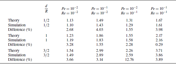


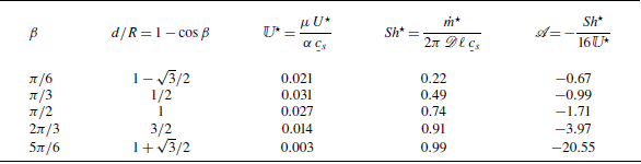


 Open access