


1. Introduction
The investigation of microchannel flows has attracted significant interest owing to their broad applications in microfluidic devices, lab-on-a-chip devices, microfluidic cooling systems, heat exchangers, microfluidic-based drug delivery systems, DNA sequencing and single-molecule detection. The use of slip microchannel flows in these applications highlights their importance in advancing innovation and improving performance across various micro- and nanofluidic technologies (Madou et al. Reference Madou, Zoval, Jia, Kido, Kim and Kim2006). Rotating micro-ducts with superhydrophobic walls have recently gained much attention because of their growing use in microfluidic devices (Chakraborty, Madou & Chakborty Reference Chakraborty, Madou and Chakborty2011), microreactor systems and point-of-care diagnostics (Hugo et al. Reference Hugo, Land, Madou and Kido2014). In such devices, rotation is often used to improve fluid mixing (Lee et al. Reference Lee, Lee, Lee, Prakash, Kim, Cho and Lee2022), particle movement and chemical reactions. Superhydrophobic surfaces (Amjad et al. Reference Amjad, Nguir, Ma and Wen2025) are commonly chosen as they reduce wall friction, resist chemical reactions and prevent fouling. The combined effect of wall slip and rotation (Chikkam & Kumar Reference Chikkam and Kumar2019) produces complex flow behaviour, which can greatly affect the onset of flow instability and transition. In these confined microchannel flows, the aspect ratio (ratio of channel height to width) also plays an important role in controlling the flow pattern and its stability. Therefore, it is essential to study the combined influence of aspect ratio, slip and rotation to achieve better design and stable performance in microfluidic systems and superhydrophobic devices (Sajjan & Raju Reference Sajjan and Raju2024). Since flow stability governs the onset of transition and mixing in such systems, a linear stability analysis provides a fundamental framework for predicting the early stages of flow disturbances and understanding their physical mechanisms.
Aspect ratio is a fundamental parameter that shapes the flow pattern in microchannels. It influences the velocity profile (Zheng & Silber-Li Reference Zheng and Silber-Li2008; Elsnab et al. Reference Elsnab, Maynes, Klewicki and Ameel2010; Prohm & Stark Reference Prohm and Stark2014), shear stress distribution and flow instabilities ( Norouzi & Biglari Reference Norouzi and Biglari2013; Jouin, Robinet & Cherubini Reference Jouin, Robinet and Cherubini2024) that may develop. The aspect ratio ( $\delta$
) is a key geometrical parameter in the design and analysis of liquid mixing in the microchannels. Microchannels are often classified as narrow or wide based on their aspect ratio, which is defined as the ratio of height to width. In the limit of a large aspect ratio, the flow approaches plane Poiseuille flow, which becomes unstable at a critical Reynolds number of
$\delta$
) is a key geometrical parameter in the design and analysis of liquid mixing in the microchannels. Microchannels are often classified as narrow or wide based on their aspect ratio, which is defined as the ratio of height to width. In the limit of a large aspect ratio, the flow approaches plane Poiseuille flow, which becomes unstable at a critical Reynolds number of $ Re_c \approx 3848$
(based on the centreline velocity, which is
$ Re_c \approx 3848$
(based on the centreline velocity, which is $1.5$
times the bulk velocity), as reported by Orszag (Reference Orszag1970). The first direct observation of flow instability was conducted by Kao & Park (Reference Kao and Park1970) using advanced experimental techniques, revealing a critical Reynolds number of approximately
$1.5$
times the bulk velocity), as reported by Orszag (Reference Orszag1970). The first direct observation of flow instability was conducted by Kao & Park (Reference Kao and Park1970) using advanced experimental techniques, revealing a critical Reynolds number of approximately $2600$
when
$2600$
when $\delta =8$
, which is significantly lower than the theoretical predictions. Tatsumi & Yoshimura (Reference Tatsumi and Yoshimura1990) depicted that duct flow becomes unstable for
$\delta =8$
, which is significantly lower than the theoretical predictions. Tatsumi & Yoshimura (Reference Tatsumi and Yoshimura1990) depicted that duct flow becomes unstable for $ \delta \gt 3.2$
, while it remains stable for
$ \delta \gt 3.2$
, while it remains stable for $ \delta \lt 3.2$
, indicating a critical aspect ratio. Their results show convergence to a plane Poiseuille instability as
$ \delta \lt 3.2$
, indicating a critical aspect ratio. Their results show convergence to a plane Poiseuille instability as $ \delta \to \infty$
. Similarly, Adachi (Reference Adachi2013) reported a critical aspect ratio of
$ \delta \to \infty$
. Similarly, Adachi (Reference Adachi2013) reported a critical aspect ratio of $ \delta = 3.19$
for rectangular ducts using bifurcation analysis. The influence of aspect ratio on the development of secondary currents in an open channel flow was also examined by Shinneeb, Nasif & Balachandar (Reference Shinneeb, Nasif and Balachandar2021), highlighting its significance in flow structure evolution. Variations in aspect ratio can alter shear distribution, boundary layer development and secondary flow patterns, all of which are critical in determining the onset and nature of flow instabilities. However, the aspect ratio in conjunction with rotation and slip effects, in the context of stability analysis, has not been examined so far.
$ \delta = 3.19$
for rectangular ducts using bifurcation analysis. The influence of aspect ratio on the development of secondary currents in an open channel flow was also examined by Shinneeb, Nasif & Balachandar (Reference Shinneeb, Nasif and Balachandar2021), highlighting its significance in flow structure evolution. Variations in aspect ratio can alter shear distribution, boundary layer development and secondary flow patterns, all of which are critical in determining the onset and nature of flow instabilities. However, the aspect ratio in conjunction with rotation and slip effects, in the context of stability analysis, has not been examined so far.
Superhydrophobic coatings are a promising way to reduce drag in applications where liquids flow over solid surfaces, spanning a broad range of Reynolds numbers from laminar to turbulent flows. In microreactors, superhydrophobic surfaces are commonly used not only because they reduce friction but also due to their strong chemical resistance. When such systems are rotated, the mixing can improve considerably, which in turn influences the residence time distribution and the consistency of the final product. Although the utilisation of microfabrication techniques employing polymeric or silicon-based materials has yielded profound insights into fluid behaviour at small scales (Ho & Tai Reference Ho and Tai1998; Stone, Stroock & Ajdari Reference Stone, Stroock and Ajdari2004), a notable phenomenon on superhydrophobic surfaces is the occurrence of velocity slip, where air trapped in micro-and nanostructures induces slip at the liquid–air interfaces for which the slip boundary condition should be adopted in modelling the problem (Choi & Kim Reference Choi and Kim2006; Lee & Kim Reference Lee and Kim2011). This slip behaviour is quantified by the effective slip length parameter, which, despite being typically minute on conventional surfaces, has been experimentally observed to reach dimensions on the order of hundreds of microns. Accurate quantification of interfacial slip was investigated by Vega-Sánchez & Neto (Reference Vega-Sánchez and Neto2022) using the pressure drop versus flow rate method. Extensive numerical and theoretical investigations have been undertaken to model velocity slip on superhydrophobic surfaces and to discern its implications for fluid transport across laminar and fully turbulent flows (Vinogradova Reference Vinogradova1999; Lauga & Stone Reference Lauga and Stone2003; Bazant & Vinogradova Reference Bazant and Vinogradova2008; Lee, Choi & Kim Reference Lee, Choi and Kim2008; Park, Park & Kim Reference Park, Park and Kim2013; Rowin & Ghaemi Reference Rowin and Ghaemi2019).
In linear stability analysis a commonly used approach is the Navier slip boundary condition, which is applied in various channel flow problems (Lauga & Cossu Reference Lauga and Cossu2005; Min & Kim Reference Min and Kim2005; Ghosh, Usha & Sahu Reference Ghosh, Usha and Sahu2014; Seo & Mani Reference Seo and Mani2016; Chai & Song Reference Chai and Song2019; Ceccacci et al. Reference Ceccacci, Calabretto, Thomas and Denier2022). Typically, slip length is considered to be uniform and isotropic, which does not vary with position or direction on the wall. Several studies have found that velocity slip stabilises the flow, thereby significantly increasing the critical Reynolds number (Lauga & Cossu Reference Lauga and Cossu2005; Min & Kim Reference Min and Kim2005; Ghosh et al. Reference Ghosh, Usha and Sahu2014). However, recent studies suggest that velocity slip can also destabilise the flow in the case of an anisotropic slip (Pralits, Alinovi & Bottaro Reference Pralits, Alinovi and Bottaro2017; Chai & Song Reference Chai and Song2019; Xiong & Tao Reference Xiong and Tao2020; Chen & Song Reference Chen and Song2021; Zhai, Chen & Song Reference Zhai, Chen and Song2023; Sengupta & Chakraborty Reference Sengupta and Chakraborty2024). Specifically, Chai & Song (Reference Chai and Song2019) revisited previous studies by Lauga & Cossu (Reference Lauga and Cossu2005) and Min & Kim (Reference Min and Kim2005), examining channel flow stability with separate streamwise and spanwise slip velocities. They demonstrated through modal and non-modal analysis that a large slip in either direction triggers three-dimensional instabilities.
Rotation of a system of fluid flow, having applications in centrifugal microfluidic devices, can enhance the instability (Alfredsson & Persson Reference Alfredsson and Persson1989; Matsson & Alfredsson Reference Matsson and Alfredsson1990; Wallin, Grundestam & Johansson Reference Wallin, Grundestam and Johansson2013; Sengupta et al. Reference Sengupta, Ghosh, Saha and Chakraborty2019a
,
Reference Sengupta, Ghosh, Saha and Chakrabortyb
, Reference Sengupta, Ghosh and Chakraborty2020). They reported that the critical Reynolds number decreased to below $100$
due to the consideration of a spanwise rotation system. Whereas Bera et al. (Reference Bera, Shit, Reza and Drese2024) illustrated the critical Reynolds number to be
$100$
due to the consideration of a spanwise rotation system. Whereas Bera et al. (Reference Bera, Shit, Reza and Drese2024) illustrated the critical Reynolds number to be $44$
at
$44$
at $Ro=0.26$
using rotating curved microchannel flows. In such systems, rotation-induced Coriolis and centrifugal forces play a pivotal role in controlling mixing, stability and transport phenomena at the microscale. Non-modal stability analyses have been carried out by Reddy & Henningson (Reference Reddy and Henningson1993), Schmid (Reference Schmid2000), Satish & Alison (Reference Satish and Alison2005), Pralits, Alinovi & Bottaro (Reference Pralits, Alinovi and Bottaro2017), Schmid, De Pando & Peake (Reference Schmid, De Pando and Peake2017), Chai & Song (Reference Chai and Song2019) and Jouin et al. (Reference Jouin, Robinet and Cherubini2024) using eigenvalues and eigenvectors to illustrate the short-term behaviour of the disturbance in terms of the transient energy growth function. These analyses give deeper insight into the disturbance, as it cannot identify any unstable modes through modal analysis.
$Ro=0.26$
using rotating curved microchannel flows. In such systems, rotation-induced Coriolis and centrifugal forces play a pivotal role in controlling mixing, stability and transport phenomena at the microscale. Non-modal stability analyses have been carried out by Reddy & Henningson (Reference Reddy and Henningson1993), Schmid (Reference Schmid2000), Satish & Alison (Reference Satish and Alison2005), Pralits, Alinovi & Bottaro (Reference Pralits, Alinovi and Bottaro2017), Schmid, De Pando & Peake (Reference Schmid, De Pando and Peake2017), Chai & Song (Reference Chai and Song2019) and Jouin et al. (Reference Jouin, Robinet and Cherubini2024) using eigenvalues and eigenvectors to illustrate the short-term behaviour of the disturbance in terms of the transient energy growth function. These analyses give deeper insight into the disturbance, as it cannot identify any unstable modes through modal analysis.
Rotating microchannel flows can lead to linear instability even at low Reynolds numbers due to the interplay between Coriolis and inertial forces. This raises an important question: Can rotation induce instability in channels with low aspect ratios ( $ \delta \lt 3.19$
), which are typically stable in the non-rotating case? Additionally, anisotropy in slip lengths where streamwise and spanwise slip differ may further influence these instabilities, potentially lowering the critical Reynolds number compared with uniformly rotating microchannels. The above-mentioned literature survey reveals a gap in the study of rotating microchannel flows, specifically in considering both the aspect ratio and wall slip simultaneously. Most earlier works focused on non-rotating flows or high-aspect-ratio channels, without considering slip effects. In this study we address this issue by analysing microchannel flows and examining how both low and high aspect ratios, as well as wall slip, affect flow stability under rotation. We employ both modal and non-modal linear stability methods. Modal analysis examines eigenvalues to determine when instability begins, while non-modal analysis investigates how disturbance energy evolves over a short time. Previous investigators mostly studied these effects separately. Following earlier works like Min & Kim (Reference Min and Kim2005), Chai & Song (Reference Chai and Song2019) and Chen & Song (Reference Chen and Song2021), we consider streamwise and spanwise slip as limiting cases of anisotropic slip, which was not considered by Sengupta & Chakraborty (Reference Sengupta and Chakraborty2024) in their recent work. To our knowledge, this is the first combined study of wall slip and aspect ratio effects on the stability of a rotating microchannel flow, and we report lower critical Reynolds numbers than those previously reported.
$ \delta \lt 3.19$
), which are typically stable in the non-rotating case? Additionally, anisotropy in slip lengths where streamwise and spanwise slip differ may further influence these instabilities, potentially lowering the critical Reynolds number compared with uniformly rotating microchannels. The above-mentioned literature survey reveals a gap in the study of rotating microchannel flows, specifically in considering both the aspect ratio and wall slip simultaneously. Most earlier works focused on non-rotating flows or high-aspect-ratio channels, without considering slip effects. In this study we address this issue by analysing microchannel flows and examining how both low and high aspect ratios, as well as wall slip, affect flow stability under rotation. We employ both modal and non-modal linear stability methods. Modal analysis examines eigenvalues to determine when instability begins, while non-modal analysis investigates how disturbance energy evolves over a short time. Previous investigators mostly studied these effects separately. Following earlier works like Min & Kim (Reference Min and Kim2005), Chai & Song (Reference Chai and Song2019) and Chen & Song (Reference Chen and Song2021), we consider streamwise and spanwise slip as limiting cases of anisotropic slip, which was not considered by Sengupta & Chakraborty (Reference Sengupta and Chakraborty2024) in their recent work. To our knowledge, this is the first combined study of wall slip and aspect ratio effects on the stability of a rotating microchannel flow, and we report lower critical Reynolds numbers than those previously reported.
2. Flow configuration and mathematical framework
We examine the stability analysis of an incompressible and rotating slip microchannel laminar flow subject to spanwise rotation. We assume that the microchannel has a half-width and half-height denoted by $d$
and
$d$
and $h$
, respectively. We use a Cartesian coordinate system
$h$
, respectively. We use a Cartesian coordinate system $(x^*, y^*, z^*)$
, where the
$(x^*, y^*, z^*)$
, where the $x^*$
axis corresponds to the streamwise direction and the
$x^*$
axis corresponds to the streamwise direction and the $y^*$
axis corresponds to the wall-normal direction. The entire system rotates about the spanwise
$y^*$
axis corresponds to the wall-normal direction. The entire system rotates about the spanwise $z^*$
direction, with a rotational velocity
$z^*$
direction, with a rotational velocity $\boldsymbol{\varOmega ^*} = (0, 0, \varOmega ^*)$
. The rotation of the microchannel system introduces the Coriolis force, represented as
$\boldsymbol{\varOmega ^*} = (0, 0, \varOmega ^*)$
. The rotation of the microchannel system introduces the Coriolis force, represented as $-2\varOmega ^* \times \mathfrak{u}^*$
, which acts as a body force. Meanwhile, the centrifugal force
$-2\varOmega ^* \times \mathfrak{u}^*$
, which acts as a body force. Meanwhile, the centrifugal force $-\varOmega ^* \times (\varOmega ^* \times r^*)$
, where
$-\varOmega ^* \times (\varOmega ^* \times r^*)$
, where $r^*$
is the position vector from the axis of rotation, is considered as a modified pressure
$r^*$
is the position vector from the axis of rotation, is considered as a modified pressure $p_m^*$
. The physical configuration of the problem is illustrated in figure 1. According to the above-mentioned assumptions, the Navier–Stokes equations system for an incompressible flow in the dimensional form is taken as
$p_m^*$
. The physical configuration of the problem is illustrated in figure 1. According to the above-mentioned assumptions, the Navier–Stokes equations system for an incompressible flow in the dimensional form is taken as
 \begin{align}& \boldsymbol{\nabla }\boldsymbol{\cdot }{\mathfrak{u}}^*=0 , \end{align}
 \begin{align} \frac {\partial {\mathfrak{u}}^*}{\partial t^*} +({\mathfrak{u}}^*\boldsymbol{\cdot }\boldsymbol{\nabla }){\mathfrak{u}}^*=&-\frac {1}{\rho }\boldsymbol{\nabla }p_m^{*}+\nu {\nabla} ^2\mathfrak{u}^*-2(\boldsymbol{\varOmega ^*} \times \mathfrak{u}^*) , \end{align}

Figure 1. Schematic diagram depicting a rotating slip microchannel flow (slip length is not possible to show due to the three-dimensional view) with a width of $2d$
and a height of
$2d$
and a height of $2h$
in figure 1(a). The mean flow is directed along the
$2h$
in figure 1(a). The mean flow is directed along the $x^*$
axis, while the entire system rotates about the
$x^*$
axis, while the entire system rotates about the $z^*$
axis. Slip lengths along both the flow (streamwise) and across the flow (spanwise and wall-normal) directions are considered due to superhydrophobicity walls, but only the streamwise slip length (
$z^*$
axis. Slip lengths along both the flow (streamwise) and across the flow (spanwise and wall-normal) directions are considered due to superhydrophobicity walls, but only the streamwise slip length ( $l_{x^*}$
) is shown as it can be clearly represented in the cross-sectional view (figure 1
b,c). Figure 1(b) displays the cross-section along
$l_{x^*}$
) is shown as it can be clearly represented in the cross-sectional view (figure 1
b,c). Figure 1(b) displays the cross-section along $y^*$
at
$y^*$
at $z^* = 0$
, showing the dimensional base-state velocity
$z^* = 0$
, showing the dimensional base-state velocity $U_1^*(y^*)$
, while figure 1(c) presents the cross-section along
$U_1^*(y^*)$
, while figure 1(c) presents the cross-section along $z^*$
at
$z^*$
at $y^* = 0$
, showing the dimensional base-state velocity
$y^* = 0$
, showing the dimensional base-state velocity $U_2^*(z^*)$
.
$U_2^*(z^*)$
.
where $\mathfrak{u}^*=(u^*,v^*,w^*)$
denotes the velocity vector and
$\mathfrak{u}^*=(u^*,v^*,w^*)$
denotes the velocity vector and $p_m^{*}=p^*-{\varOmega ^*}^2(x^{*^2}+y^{*^2})$
the modified pressure.
$p_m^{*}=p^*-{\varOmega ^*}^2(x^{*^2}+y^{*^2})$
the modified pressure.
In the presence of hydrophobic walls, we employ the following Navier slip boundary conditions for velocity components:
 \begin{align}& u^*\pm l_{x^*}\frac {\partial u^*}{\partial y^*}=0,\qquad w^*\pm l_{z^*}\frac {\partial w^*}{\partial y^*}=0\quad \mbox{and}\quad v^*=0 \hspace {0.5cm} \mbox{at} \,\, y^*=\pm d,\nonumber \\& u^*\pm l_{x^*}\frac {\partial u^*}{\partial z^*}=0,\qquad v^*\pm l_{y^*}\frac {\partial v^*}{\partial z^*}=0\quad\mbox{and}\quad w^*=0 \hspace {0.5cm} \mbox{at}\,\, z^*=\pm h. \end{align}
Here $l_{x^*}$
,
$l_{x^*}$
, $l_{y^*}$
and
$l_{y^*}$
and $l_{z^*}$
are the streamwise, wall-normal and spanwise slip lengths, and they are independent of each other. Here, we consider the symmetric slip lengths, which are the same on all the walls.
$l_{z^*}$
are the streamwise, wall-normal and spanwise slip lengths, and they are independent of each other. Here, we consider the symmetric slip lengths, which are the same on all the walls.
2.1. Base flow characteristics
Owing to the above-mentioned flow configuration, we decompose the velocity and pressure into steady and unsteady disturbances of a fully developed base flow as
 \begin{align} \mathfrak{u}^*(x^*,y^*,z^*,t^*)&=U^*(x^*,y^*,z^*)+\tilde {\mathfrak{u}}^*(x^*,y^*,z^*,t^*),\hspace {0.35cm}\nonumber \\ p_{m}^*(x^*,y^*,z^*,t^*)&=P^*(x^*,y^*,z^*)+\tilde {p}^*(x^*,y^*,z^*,t^*), \end{align}
where the variables with $(^*)$
define the dimensional perturbed quantities in which
$(^*)$
define the dimensional perturbed quantities in which $\tilde {\mathfrak{u}}^*(\tilde {u}^*,\tilde {v}^*,\tilde {w}^*)$
and
$\tilde {\mathfrak{u}}^*(\tilde {u}^*,\tilde {v}^*,\tilde {w}^*)$
and $\tilde {p}^*$
are very small. We express the governing equations in non-dimensional form using the scaling variables
$\tilde {p}^*$
are very small. We express the governing equations in non-dimensional form using the scaling variables
 \begin{align} &\mathfrak{u}=\frac {\tilde {\mathfrak{u}}^*}{U_b},\quad U=\frac {U^*}{U_b},\quad l_x=\frac {l_{x^*}}{D_H},\quad l_{\!y}=\frac {2\delta }{1+\delta }\frac {l_{y^*}}{D_H},\quad l_z=\frac {2}{1+\delta }\frac {l_{z^*}}{D_H},\quad \delta =\frac {h}{d}, \hspace {0cm}\nonumber \\& x=\frac {x^*}{D_H}, \quad y=\frac {2\delta }{1+\delta }\frac {y^*}{D_H}, \quad z=\frac {2}{1+\delta }\frac {z^*}{D_H}, \quad t=\frac {t^*}{T}, \quad p=\frac {\tilde {p}^*}{\rho U_b^2},\end{align}
where $\delta$
is the aspect ratio of the rectangular channel and
$\delta$
is the aspect ratio of the rectangular channel and $D_H= 2hd/({h+d} )$
is the hydraulic diameter of the channel,
$D_H= 2hd/({h+d} )$
is the hydraulic diameter of the channel, $l_x$
,
$l_x$
, $l_{\!y}$
and
$l_{\!y}$
and $l_z$
represent the dimensionless slip lengths (Knudsen number) in the streamwise, wall-normal and spanwise directions, respectively;
$l_z$
represent the dimensionless slip lengths (Knudsen number) in the streamwise, wall-normal and spanwise directions, respectively; $T$
is the real mixing time and
$T$
is the real mixing time and $U_b$
denotes the bulk (or mean) velocity. It is important to note that the base-state velocity is influenced only by the streamwise slip
$U_b$
denotes the bulk (or mean) velocity. It is important to note that the base-state velocity is influenced only by the streamwise slip $l_x$
(Chai & Song Reference Chai and Song2019; Chen & Song Reference Chen and Song2021).
$l_x$
(Chai & Song Reference Chai and Song2019; Chen & Song Reference Chen and Song2021).
By considering $\mathfrak{u}^*=(U^*(y^*,z^*),0,0)$
, which satisfies the continuity equation (2.1) automatically and then applying the dimensionless quantities defined in (2.5) into the momentum (2.2), the governing equation for base flow for an incompressible and steady flow reads
$\mathfrak{u}^*=(U^*(y^*,z^*),0,0)$
, which satisfies the continuity equation (2.1) automatically and then applying the dimensionless quantities defined in (2.5) into the momentum (2.2), the governing equation for base flow for an incompressible and steady flow reads
 \begin{equation} \left (\frac {2\delta }{1+\delta }\right )^2\frac {\partial ^2U}{\partial y^2}+\left (\frac {2}{1+\delta }\right )^2\frac {\partial ^2U}{\partial z^2}={\textit{Re}}\frac {\textrm{d}P}{\textrm{d}x},\quad v=0,\quad w=0, \end{equation}
which is then transformed to
 \begin{equation} \frac {\partial ^2U}{\partial y^2}+\frac {1}{\delta ^2}\frac {\partial ^2U}{\partial z^2}={\textit{Re}}\frac {\textrm{d}P}{\textrm{d}x}\left (\frac {1+\delta }{2\delta }\right )^2. \end{equation}
The boundary conditions (see (2.3)) for the base flow become
 \begin{align}& U+l_x\frac {\partial U}{\partial y}=0\quad\mbox{at}\ y= 1;\qquad U-l_x\frac {\partial U}{\partial y}=0 \hspace {0.5cm} \mbox{at}\,\, y=-1,\nonumber \\& U+l_x \frac {\partial U}{\partial z}=0\quad \mbox{at}\ z= 1;\qquad U-l_x\frac {\partial U}{\partial z}=0 \hspace {0.5cm} \mbox{at}\,\, z=-1, \end{align}
where the Reynolds number is defined as ${\textit{Re}}=(U_bD_H)/{\nu }$
. In order to solve (2.7) subject to the boundary condition (2.8), we use the Chebyshev differentiation matrix (Trefethen Reference Trefethen2000) along with the tensor product from linear algebra, the left-hand side of (2.7) follows
${\textit{Re}}=(U_bD_H)/{\nu }$
. In order to solve (2.7) subject to the boundary condition (2.8), we use the Chebyshev differentiation matrix (Trefethen Reference Trefethen2000) along with the tensor product from linear algebra, the left-hand side of (2.7) follows
 \begin{equation} (I\otimes {\mathcal{D}}^2)+\frac {1}{\delta ^2}\times ({\mathcal{D}}^2\otimes I), \end{equation}
where $\mathcal{D}^2$
represents the second-order Chebyshev differentiation matrix. Using the matrix inversion method, we solve (2.7) and extract a cross-sectional profile along the line
$\mathcal{D}^2$
represents the second-order Chebyshev differentiation matrix. Using the matrix inversion method, we solve (2.7) and extract a cross-sectional profile along the line $z=0$
, which varies with the wall-normal direction
$z=0$
, which varies with the wall-normal direction $y$
as well as along the line
$y$
as well as along the line $y=0$
, which varies along the direction
$y=0$
, which varies along the direction $z$
. We reduce the resulting steady base flow in dimensionless form using the mean velocity and use the same length scales of
$z$
. We reduce the resulting steady base flow in dimensionless form using the mean velocity and use the same length scales of $y$
and
$y$
and $z$
as depicted in figure 2(a) depending on
$z$
as depicted in figure 2(a) depending on $y$
, and in figure 2(b) depending on
$y$
, and in figure 2(b) depending on $z$
with a varying aspect ratio (
$z$
with a varying aspect ratio ( $\delta$
). To make the scales comparable for plotting
$\delta$
). To make the scales comparable for plotting $U_1$
and
$U_1$
and $U_2$
, we normalise the length scales to
$U_2$
, we normalise the length scales to $[-1,1]$
. As a result of this rescaling, the maximum values of
$[-1,1]$
. As a result of this rescaling, the maximum values of $U_1$
and
$U_1$
and $U_2$
appear different even for the same aspect ratio. This difference arises solely from the normalisation of the axes for comparison and does not affect the physical behaviour of the base flow. Since the base flow is non-dimensionalised using the mean velocity, the maximum velocity becomes
$U_2$
appear different even for the same aspect ratio. This difference arises solely from the normalisation of the axes for comparison and does not affect the physical behaviour of the base flow. Since the base flow is non-dimensionalised using the mean velocity, the maximum velocity becomes $\approx 1.5$
. From both the figures, we state that the aspect ratio (
$\approx 1.5$
. From both the figures, we state that the aspect ratio ( $\delta = h/d$
) plays a crucial role in shaping the base flow velocity profiles
$\delta = h/d$
) plays a crucial role in shaping the base flow velocity profiles $U_1(y)$
and
$U_1(y)$
and $U_2(z)$
for fully developed laminar flow in a channel and thereby impacts the stability of the flow. At low aspect ratios (
$U_2(z)$
for fully developed laminar flow in a channel and thereby impacts the stability of the flow. At low aspect ratios ( $\delta \lt 1$
), the channel is wide and shallow. In this case, the velocity profile becomes flattened along
$\delta \lt 1$
), the channel is wide and shallow. In this case, the velocity profile becomes flattened along $y$
due to the weaker influence of the vertical boundaries, while along
$y$
due to the weaker influence of the vertical boundaries, while along $z$
, the velocity profile becomes parabolic-like, similar to that of an infinite parallel plate, due to the strong viscous effects of the horizontal boundaries. On the other hand, when the aspect ratio is greater than one (
$z$
, the velocity profile becomes parabolic-like, similar to that of an infinite parallel plate, due to the strong viscous effects of the horizontal boundaries. On the other hand, when the aspect ratio is greater than one ( $\delta \gt 1$
), the channel deepens. Here, we observe exactly the opposite trend in the velocity profile due to the stronger viscous effect of the vertical walls, which exhibits a parabolic profile along
$\delta \gt 1$
), the channel deepens. Here, we observe exactly the opposite trend in the velocity profile due to the stronger viscous effect of the vertical walls, which exhibits a parabolic profile along $y$
that flattens along
$y$
that flattens along $z$
. This may have a different effect on the stability of rotating microchannel flows.
$z$
. This may have a different effect on the stability of rotating microchannel flows.

Figure 2. The base-state velocity profile, incorporating streamwise slip ( $l_x = 0.02$
), is plotted for different aspect ratios (
$l_x = 0.02$
), is plotted for different aspect ratios ( $\delta = h/d$
). Specifically, panel (a) represents the wall-normal base flow by setting
$\delta = h/d$
). Specifically, panel (a) represents the wall-normal base flow by setting $ z = 0$
, while panel (b) corresponds to the spanwise base flow by setting
$ z = 0$
, while panel (b) corresponds to the spanwise base flow by setting $ y = 0$
. These profiles provide insights into the influence of aspect ratio on the base-state velocity distribution under slip conditions. The discrepancy in the magnitude of velocity between (a) and (b) is due to the reduction of the length scale along the
$ y = 0$
. These profiles provide insights into the influence of aspect ratio on the base-state velocity distribution under slip conditions. The discrepancy in the magnitude of velocity between (a) and (b) is due to the reduction of the length scale along the $y$
and
$y$
and $z$
directions to
$z$
directions to $[-1,1]$
.
$[-1,1]$
.
To better capture the effects of aspect ratio and its interaction with rotation, we formulate the linear stability equations separately in terms of the $ y$
and
$ y$
and $ z$
directions. For aspect ratios
$ z$
directions. For aspect ratios $\delta \gt 1$
, the computational domain is defined as
$\delta \gt 1$
, the computational domain is defined as $[-1,1] \times [-\delta , \delta ]$
, whereas for
$[-1,1] \times [-\delta , \delta ]$
, whereas for $\delta \lt 1$
, the domain is chosen as
$\delta \lt 1$
, the domain is chosen as $[-(1/\delta), ( {1}/{\delta })] \times [-1,1]$
. For the unit aspect ratio case (
$[-(1/\delta), ( {1}/{\delta })] \times [-1,1]$
. For the unit aspect ratio case ( $\delta = 1$
), we present results using one-dimensional base states along both wall-normal and spanwise directions. These represent two orthogonal shear configurations in a square duct. The close agreement in the qualitative stability trends obtained from these two independent analyses gives confidence in the physical interpretation of the results. However, we note that a full two-dimensional base flow may be required for more precise quantitative results near
$\delta = 1$
), we present results using one-dimensional base states along both wall-normal and spanwise directions. These represent two orthogonal shear configurations in a square duct. The close agreement in the qualitative stability trends obtained from these two independent analyses gives confidence in the physical interpretation of the results. However, we note that a full two-dimensional base flow may be required for more precise quantitative results near $\delta \approx 1$
. This approach ensures that the hydraulic diameter of the channel remains unchanged, while allowing for a more precise analysis of stability characteristics across different aspect ratios.
$\delta \approx 1$
. This approach ensures that the hydraulic diameter of the channel remains unchanged, while allowing for a more precise analysis of stability characteristics across different aspect ratios.
2.2. Wall-normal linear stability equations
Taking into account the viscous effects of the walls at $ y^* = -d$
and
$ y^* = -d$
and $ y^* = +d$
, we consider the wall-normal base velocity
$ y^* = +d$
, we consider the wall-normal base velocity $ U_1^*(y^*)$
. In this case, the base-state velocity is treated as a function of
$ U_1^*(y^*)$
. In this case, the base-state velocity is treated as a function of $ y^* \in [-d,d]$
only, as illustrated in figure 2(a). Then with a small disturbance
$ y^* \in [-d,d]$
only, as illustrated in figure 2(a). Then with a small disturbance $(\tilde {u}^*,\tilde {v}^*,\tilde {w}^*)$
the fully developed base velocity
$(\tilde {u}^*,\tilde {v}^*,\tilde {w}^*)$
the fully developed base velocity $(U_1^*(y^*),0,0)$
changes to
$(U_1^*(y^*),0,0)$
changes to $(U_1^*(y^*)+\tilde {u}^*,\tilde {v}^*,\tilde {w}^*)$
. By substituting the perturbed velocity into the governing equations (2.1) and (2.2) and linearising the equations for the small disturbance, we obtain the following dimensionless mass and momentum balance equations that govern the perturbed flow in the reference frame of the rotating microchannel:
$(U_1^*(y^*)+\tilde {u}^*,\tilde {v}^*,\tilde {w}^*)$
. By substituting the perturbed velocity into the governing equations (2.1) and (2.2) and linearising the equations for the small disturbance, we obtain the following dimensionless mass and momentum balance equations that govern the perturbed flow in the reference frame of the rotating microchannel:
 \begin{align}&\qquad\qquad\qquad\qquad\qquad \frac {\partial u}{\partial x}+\frac {\partial v}{\partial y}+\left (\frac {2}{1+\delta }\right )\frac {\partial w}{\partial z}=0 , \end{align}
 \begin{align}& \frac {\partial u}{\partial t}+U_1\frac {\partial u}{\partial x}+ \frac {\partial U_1}{\partial y}v=-\frac {\partial p}{\partial x} +\frac {1}{\textit{Re}}\left [\frac {\partial ^2 u}{\partial x^2}+\frac {\partial ^2 u}{\partial y^2}+\left (\frac {2}{1+\delta }\right )^2\frac {\partial ^2 u}{\partial z^2}\right ]+({\textit{Ro}})v, \end{align}
 \begin{align}&\qquad \frac {\partial v}{\partial t}+U_1\frac {\partial v}{\partial x}=-\frac {\partial p}{\partial y} +\frac {1}{\textit{Re}}\left [\frac {\partial ^2 v}{\partial x^2}+ \frac {\partial ^2 v}{\partial y^2}+\left (\frac {2}{1+\delta }\right )^2\frac {\partial ^2 v}{\partial z^2}\right ]-({\textit{Ro}}) u, \end{align}
 \begin{align}&\quad \frac {\partial w}{\partial t}+U_1\frac {\partial w}{\partial x} =-\left (\frac {2}{1+\delta }\right )\frac {\partial p}{\partial z}+\frac {1}{\textit{Re}}\left [\frac {\partial ^2 w}{\partial x^2}+ \frac {\partial ^2 w}{\partial y^2}+\left (\frac {2}{1+\delta }\right )^2\frac {\partial ^2 w}{\partial z^2}\right ]\!. \\[9pt] \nonumber \end{align}
Then $y\in [-1,1]$
and the slip boundary conditions at the walls
$y\in [-1,1]$
and the slip boundary conditions at the walls $(y=\pm 1$
) reduce to
$(y=\pm 1$
) reduce to
 \begin{align}& u+l_x \frac {\partial u}{\partial y}=0,\qquad w+l_z \frac {\partial w}{\partial y}=0\quad \mbox{and}\quad v=0 \mbox{ at }y=1, \nonumber \\& u-l_x \frac {\partial u}{\partial y}=0,\qquad w-l_z \frac {\partial w}{\partial y}=0\quad \mbox{and}\quad v=0 \mbox{ at } y=-1. \end{align}
Now (2.10)–(2.13) reform into a set of coupled differential equations in terms of velocity $v$
and vorticity
$v$
and vorticity $\eta =( {\partial u}/{\partial z})-( {\partial w}/{\partial x})$
, i.e.
$\eta =( {\partial u}/{\partial z})-( {\partial w}/{\partial x})$
, i.e.
 \begin{align}& \frac {\partial }{\partial t} ({\nabla} ^2 v)+U_1\frac {\partial }{\partial x}({\nabla} ^2v)-U_1'' \frac {\partial v}{\partial x} = \frac {1}{\textit{Re}} ({\nabla} ^4 v)-Ro\left (\frac {2}{1+\delta }\right )\frac {\partial \eta }{\partial z}, \end{align}
 \begin{align}&\,\,\, \frac {\partial \eta }{\partial t}+U_1\frac {\partial \eta }{\partial x}+U_1'\left (\frac {2}{1+\delta }\right )\frac {\partial v}{\partial z} =\frac {1}{\textit{Re}} ({\nabla} ^2 \eta)+ Ro\left (\frac {2}{1+\delta }\right )\frac {\partial v}{\partial z}, \end{align}
with the following revised boundary conditions in terms of $v$
and
$v$
and $\eta$
:
$\eta$
:
 \begin{gather} v= D_1v+l D_1^2v=0 \quad \mbox{at } y=1;\qquad v= D_1v-l D_1^2v=0 \quad \mbox{at } y=-1, \nonumber \\ \eta +l D_1 \eta =0\quad \mbox{at } y=1; \qquad \eta -l D_1\eta =0 \quad \mbox{at } y=-1. \end{gather}
Here $l=l_x=l_z$
is the isotropic and symmetric slip length. The derivative operator
$l=l_x=l_z$
is the isotropic and symmetric slip length. The derivative operator $D_1$
along
$D_1$
along $y$
, Reynolds number (
$y$
, Reynolds number ( ${\textit{Re}}$
) and rotation number (
${\textit{Re}}$
) and rotation number ( $Ro$
) are respectively defined as:
$Ro$
) are respectively defined as:
 \begin{align} \hspace {1.5cm} D_1\equiv {\frac {\textrm{d}}{\textrm{d}y}}, \qquad {\textit{Re}}=\frac {U_bD_H}{\nu }, \qquad Ro=\frac {2\varOmega ^* D_H}{U_b}. \end{align}
For linear stability analysis of the present study, we introduce the normal mode assumption in the form
 \begin{equation} \begin{pmatrix} v(x,y,z,t) \\ \eta (x,y,z,t) \end{pmatrix} =\begin{pmatrix} \tilde {v}(y) \\ \tilde {\eta }(y) \end{pmatrix}\exp [i(\alpha x+\beta _1 z-\omega t)], \end{equation}
where the variables $\tilde v$
and
$\tilde v$
and $\tilde \eta$
denote the amplitude corresponding to the perturbation wave of wall-normal velocity and vorticity. Moreover,
$\tilde \eta$
denote the amplitude corresponding to the perturbation wave of wall-normal velocity and vorticity. Moreover, $\alpha$
and
$\alpha$
and $\beta _1$
represent the streamwise and spanwise wavenumbers, respectively. To ensure a proper fit to the chosen domain based on the aspect ratio, the spanwise wavenumber
$\beta _1$
represent the streamwise and spanwise wavenumbers, respectively. To ensure a proper fit to the chosen domain based on the aspect ratio, the spanwise wavenumber $\beta _1$
is scaled by a factor of
$\beta _1$
is scaled by a factor of $ (1+\delta)/{2\delta }$
. This scaling accounts for variations in the domain size, ensuring consistency in the representation of spanwise disturbances across different aspect ratios. The temporal frequency is
$ (1+\delta)/{2\delta }$
. This scaling accounts for variations in the domain size, ensuring consistency in the representation of spanwise disturbances across different aspect ratios. The temporal frequency is $\omega (\alpha ,\beta _1)$
, where
$\omega (\alpha ,\beta _1)$
, where $(\omega =\omega _r +i\omega _i)$
is the frequency of the disturbance. Applying the normal mode of variables
$(\omega =\omega _r +i\omega _i)$
is the frequency of the disturbance. Applying the normal mode of variables $v$
and
$v$
and $\eta$
defined in (2.19) into (2.15) and (2.16). Then, a coupled Orr–Sommerfield–Squire system is obtained in the matrix form given by
$\eta$
defined in (2.19) into (2.15) and (2.16). Then, a coupled Orr–Sommerfield–Squire system is obtained in the matrix form given by
 \begin{equation} -i\omega \underbrace {\begin{pmatrix} B^1_{11} & 0 \\ 0 & B^1_{22} \end{pmatrix}}_{B_1} \underbrace {\begin{pmatrix} \tilde v \\ \tilde {\eta } \end{pmatrix}}_{q_1} =\underbrace {\begin{pmatrix} A^1_{11} & A^1_{12}\\ A^1_{21} & A^1_{22} \end{pmatrix}}_{A_1} \underbrace {\begin{pmatrix} \tilde v \\ \tilde {\eta } \end{pmatrix}}_{q_1}\!. \end{equation}
The above-mentioned operators are defined as
 \begin{gather} A^1_{11}=\frac {\varDelta _1^2}{\textit{Re}}-i\alpha U_1\varDelta _1 +i\alpha U_1'';\qquad A^1_{12}=-i\frac {1}{\delta }\beta _1 Ro, \nonumber \\ A^1_{21}=i\frac {1}{\delta }\beta _1\left [Ro- U_1'\right ];\qquad A^1_{22}=\frac {\varDelta _1}{\textit{Re}}-i\alpha U_1,\qquad \nonumber \\ B^1_{11}=\varDelta _1 ;\qquad B^1_{22}=I, \end{gather}
where $\varDelta _1^2=D_1^2-(\alpha ^2+({ {\beta _1^2}/{\delta ^2}}))$
and
$\varDelta _1^2=D_1^2-(\alpha ^2+({ {\beta _1^2}/{\delta ^2}}))$
and $I$
are the identity matrices. The matrix equation (2.20) along with the six boundary conditions (2.17) provided a fourth-order eigenvalue problem and has the representation of the form
$I$
are the identity matrices. The matrix equation (2.20) along with the six boundary conditions (2.17) provided a fourth-order eigenvalue problem and has the representation of the form $-i\omega B_1q_1=A_1q_1$
. This eigenvalue problem is solved by the Chebyshev spectral collocation method (Schmid & Henningson Reference Schmid and Henningson2001).
$-i\omega B_1q_1=A_1q_1$
. This eigenvalue problem is solved by the Chebyshev spectral collocation method (Schmid & Henningson Reference Schmid and Henningson2001).
2.3. Spanwise linear stability equations
Similarly, by accounting for the viscous effects of the vertical walls at $ z^* = -h$
and
$ z^* = -h$
and $ z^* = +h$
, we consider the spanwise base velocity
$ z^* = +h$
, we consider the spanwise base velocity $ {U_2}^*(z^*)$
. Consequently, the base-state velocity is treated as a function of
$ {U_2}^*(z^*)$
. Consequently, the base-state velocity is treated as a function of $ z^* \in [-h,h]$
only, as illustrated in figure 2(b). Then with a small disturbance
$ z^* \in [-h,h]$
only, as illustrated in figure 2(b). Then with a small disturbance $(\tilde {u}^*,\tilde {v}^*,\tilde {w}^*)$
the fully developed base velocity
$(\tilde {u}^*,\tilde {v}^*,\tilde {w}^*)$
the fully developed base velocity $(U_2^*(z^*),0,0)$
changes to
$(U_2^*(z^*),0,0)$
changes to $(U_2^*(z^*)+\tilde {u}^*,\tilde {v}^*,\tilde {w}^*)$
. By substituting the perturbed velocity into the governing equations (2.1) and (2.2) and linearising the equations for the small disturbance, we obtain the following dimensionless mass and momentum balance equations that govern the perturbed flow in the reference frame of the rotating microchannel:
$(U_2^*(z^*)+\tilde {u}^*,\tilde {v}^*,\tilde {w}^*)$
. By substituting the perturbed velocity into the governing equations (2.1) and (2.2) and linearising the equations for the small disturbance, we obtain the following dimensionless mass and momentum balance equations that govern the perturbed flow in the reference frame of the rotating microchannel:
 \begin{align}&\qquad\qquad\qquad\qquad\qquad \frac {\partial u}{\partial x}+\left (\frac {2\delta }{1+\delta }\right )\frac {\partial v}{\partial y}+\frac {\partial w}{\partial z}=0 , \end{align}
 \begin{align}& \frac {\partial u}{\partial t}+U_2\frac {\partial u}{\partial x}+ \frac {\partial U_2}{\partial z}w=-\frac {\partial p}{\partial x} +\frac {1}{\textit{Re}}\left [\frac {\partial ^2 u}{\partial x^2}+\left (\frac {2\delta }{1+\delta }\right )^2\frac {\partial ^2 u}{\partial y^2}+\frac {\partial ^2 u}{\partial z^2}\right ]+({\textit{Ro}}) v, \end{align}
 \begin{align}& \frac {\partial v}{\partial t}+U_2\frac {\partial v}{\partial x}=-\left (\frac {2\delta }{1+\delta }\right )\frac {\partial p}{\partial y} +\frac {1}{\textit{Re}}\left [\frac {\partial ^2 v}{\partial x^2}+ \left (\frac {2\delta }{1+\delta }\right )^2\frac {\partial ^2 v}{\partial y^2}+\frac {\partial ^2 v}{\partial z^2}\right ]-({\textit{Ro}}) u, \end{align}
 \begin{align}&\qquad\qquad \frac {\partial w}{\partial t}+U_2\frac {\partial w}{\partial x} =-\frac {\partial p}{\partial z}+\frac {1}{\textit{Re}}\left [\frac {\partial ^2 w}{\partial x^2}+ \left (\frac {2\delta }{1+\delta }\right )^2\frac {\partial ^2 w}{\partial y^2}+\frac {\partial ^2 w}{\partial z^2}\right ]\!. \end{align}
Then $z\in [-1,1]$
and the slip boundary conditions at the walls
$z\in [-1,1]$
and the slip boundary conditions at the walls $(z=\pm 1$
) reduce to
$(z=\pm 1$
) reduce to
 \begin{align}& u+l_x \frac {\partial u}{\partial z}=0,\qquad v+l_{\!y} \frac {\partial v}{\partial z}=0\quad \mbox{and}\quad w=0 \,\mbox{at}\,z=1, \nonumber \\& u-l_x \frac {\partial u}{\partial z}=0,\qquad v-l_{\!y} \frac {\partial v}{\partial z}=0\quad \mbox{and}\quad w=0 \,\mbox{at}\, z=-1. \end{align}
Now (2.22)–(2.25) reform into a set of coupled differential equations in terms of velocity $w$
and vorticity
$w$
and vorticity $\zeta =( {\partial v}/{\partial x})-( {\partial u}/{\partial y})$
, i.e.
$\zeta =( {\partial v}/{\partial x})-( {\partial u}/{\partial y})$
, i.e.
 \begin{align}& \frac {\partial }{\partial t} ({\nabla} ^2 w)+U_2\frac {\partial }{\partial x}({\nabla} ^2w)-{U_2}'' \frac {\partial w}{\partial x} = \frac {1}{\textit{Re}} ({\nabla} ^4 w)-Ro\frac {\partial \zeta }{\partial z}, \end{align}
 \begin{align}&\,\,\, \frac {\partial \zeta }{\partial t}+U_2\frac {\partial \zeta }{\partial x}-{U_2}'\left (\frac {2\delta }{1+\delta }\right )\frac {\partial w}{\partial y} =\frac {1}{\textit{Re}} ({\nabla} ^2 \zeta)+ Ro\frac {\partial w}{\partial z}, \end{align}
with the following revised boundary conditions in terms of $v$
and
$v$
and $\eta$
:
$\eta$
:
 \begin{align}& w= D_2w+l D_2^2w=0 \quad \mbox{at } z=1;\qquad w= D_2w-l D_2^2w=0 \quad \mbox{at} \hspace {0.1cm} z=-1, \end{align}
 \begin{align}&\qquad\qquad \zeta +l D_2 \zeta =0\quad \mbox{at} \hspace {0.1cm} z=1;\qquad \zeta -l D_2\zeta =0 \quad \mbox{at} \hspace {0.1cm}z=-1. \end{align}
Here $l=l_x=l_{\!y}$
is an isotropic and symmetric slip length. The derivative operator
$l=l_x=l_{\!y}$
is an isotropic and symmetric slip length. The derivative operator $D_2$
, Reynolds number (
$D_2$
, Reynolds number ( ${\textit{Re}}$
) and rotation number (
${\textit{Re}}$
) and rotation number ( $Ro$
) are respectively written as
$Ro$
) are respectively written as
 \begin{align} \hspace {1.5cm} D_2\equiv {\frac {\mathrm{d}}{\textrm{d}z}}, \qquad {\textit{Re}}=\frac {U_bD_H}{\nu }, \qquad Ro=\frac {2\varOmega ^* D_H}{U_b}. \end{align}
For linear stability analysis of the present study, we introduce the normal mode assumption in the form
 \begin{equation} \begin{pmatrix} w(x,y,z,t) \\ \zeta (x,y,z,t) \end{pmatrix} =\begin{pmatrix} \tilde {w}(z) \\ \tilde {\zeta }(z) \end{pmatrix}\exp [i(\alpha x+\beta _2 y-\omega t)], \end{equation}
where variables $\tilde w$
and
$\tilde w$
and $\tilde \zeta$
denote the amplitude corresponding to the perturbation wave of velocity (
$\tilde \zeta$
denote the amplitude corresponding to the perturbation wave of velocity ( $w$
) and vorticity (
$w$
) and vorticity ( $\zeta$
). Moreover,
$\zeta$
). Moreover, $\beta _2$
represents the spanwise wavenumber, which is scaled by a factor of
$\beta _2$
represents the spanwise wavenumber, which is scaled by a factor of $ (1+\delta)/{2}$
to ensure consistency with the chosen domain based on the aspect ratio. Additionally, the temporal frequency
$ (1+\delta)/{2}$
to ensure consistency with the chosen domain based on the aspect ratio. Additionally, the temporal frequency $\omega (\alpha ,\beta _2)$
, (
$\omega (\alpha ,\beta _2)$
, ( $\omega = \omega _r + i\omega _i$
) characterises the disturbance, where
$\omega = \omega _r + i\omega _i$
) characterises the disturbance, where $\omega _r$
corresponds to the oscillatory behaviour and
$\omega _r$
corresponds to the oscillatory behaviour and $\omega _i$
determines the growth or decay of the perturbation over time. By applying the normal mode of variables
$\omega _i$
determines the growth or decay of the perturbation over time. By applying the normal mode of variables $w$
and
$w$
and $\zeta$
defined in (2.32) into (2.27) and (2.28), a coupled Orr-Sommerfield-Squire system is then obtained in the matrix form
$\zeta$
defined in (2.32) into (2.27) and (2.28), a coupled Orr-Sommerfield-Squire system is then obtained in the matrix form
 \begin{equation} -i\omega \underbrace {\begin{pmatrix} B^2_{11} & 0 \\ 0 & B^2_{22} \end{pmatrix}}_{B_2} \underbrace {\begin{pmatrix} \tilde w \\ \tilde {\zeta } \end{pmatrix}}_{q_2} =\underbrace {\begin{pmatrix} A^2_{11} & A^2_{12}\\ A^2_{21} & A^2_{22} \end{pmatrix}}_{A_2} \underbrace {\begin{pmatrix} \tilde w \\ \tilde {\zeta } \end{pmatrix}}_{q_2}\!. \end{equation}
The above-mentioned operators are defined as
 \begin{gather} A^2_{11}=\frac {\varDelta _2^2}{\textit{Re}}-i\alpha U_2\varDelta _2+i\alpha U_2'';\qquad A^2_{12}= -RoD_2, \nonumber \\ A^2_{21}=RoD_2+i\delta \beta _2 U_2';\qquad A^2_{22}=\frac {\varDelta _2}{\textit{Re}}-i\alpha U_2, \nonumber \\ B^2_{11}=\varDelta _2 ;\qquad B^2_{22}=I, \end{gather}
where $\varDelta _2^2=D_2^2-(\alpha ^2+\delta ^2{\beta _2}^2)$
and
$\varDelta _2^2=D_2^2-(\alpha ^2+\delta ^2{\beta _2}^2)$
and $I$
are the identity matrices. The matrix equation (2.33) along with the six boundary conditions ((2.29), (2.30)) provides a fourth-order eigenvalue problem and has the representation of the form
$I$
are the identity matrices. The matrix equation (2.33) along with the six boundary conditions ((2.29), (2.30)) provides a fourth-order eigenvalue problem and has the representation of the form $-i\omega B_2q_2=A_2q_2$
. This eigenvalue problem is solved by the Chebyshev spectral collocation method (Schmid & Henningson Reference Schmid and Henningson2001).
$-i\omega B_2q_2=A_2q_2$
. This eigenvalue problem is solved by the Chebyshev spectral collocation method (Schmid & Henningson Reference Schmid and Henningson2001).
3. Validation of the present results
We solve the eigenvalue problems given in (2.20) and (2.33) numerically to obtain the eigenvalues and eigenvectors of the wall-normal and spanwise operators. To validate our numerical code, we compute the growth rate of the most unstable modes for no-slip, non-rotating channel flows with $\alpha =0.91$
and an aspect ratio of
$\alpha =0.91$
and an aspect ratio of $\delta =5$
. Then, the computed results are compared with those of Adachi (Reference Adachi2013), as shown in figure 3(a). Figure 3(b) also presents a validation of our computational results incorporating slip boundary conditions at the wall, by comparing them with the findings of Ghosh et al. (Reference Ghosh, Usha and Sahu2014) for the non-rotating case (
$\delta =5$
. Then, the computed results are compared with those of Adachi (Reference Adachi2013), as shown in figure 3(a). Figure 3(b) also presents a validation of our computational results incorporating slip boundary conditions at the wall, by comparing them with the findings of Ghosh et al. (Reference Ghosh, Usha and Sahu2014) for the non-rotating case ( $Ro = 0.0$
). In both cases, the maximum velocity of the base flow is normalised to unity. These results show a good agreement with those of Adachi (Reference Adachi2013) and Ghosh et al. (Reference Ghosh, Usha and Sahu2014), who studied a special case of the present study.
$Ro = 0.0$
). In both cases, the maximum velocity of the base flow is normalised to unity. These results show a good agreement with those of Adachi (Reference Adachi2013) and Ghosh et al. (Reference Ghosh, Usha and Sahu2014), who studied a special case of the present study.

Figure 3. (a) Comparison of the maximum growth rate for non-rotating ( $Ro=0.0$
) flow in a microchannel, when we set
$Ro=0.0$
) flow in a microchannel, when we set $\delta =5,\,\alpha =0.91$
and
$\delta =5,\,\alpha =0.91$
and $l=0.0$
. (b) Comparison of the critical Reynolds number depending on slip length, with the results of Ghosh et al. (Reference Ghosh, Usha and Sahu2014) in the case of a non-rotating system when
$l=0.0$
. (b) Comparison of the critical Reynolds number depending on slip length, with the results of Ghosh et al. (Reference Ghosh, Usha and Sahu2014) in the case of a non-rotating system when $\delta =1$
. In the setting of these parameters in the present computational study, we find physical alignment with those of Adachi (Reference Adachi2013) and Ghosh et al. (Reference Ghosh, Usha and Sahu2014).
$\delta =1$
. In the setting of these parameters in the present computational study, we find physical alignment with those of Adachi (Reference Adachi2013) and Ghosh et al. (Reference Ghosh, Usha and Sahu2014).

Figure 4. Comparison of the maximum growth rates versus aspect ratio between non-rotating and rotating cases from both wall-normal and spanwise modes at ${\textit{Re}} = 200$
, when
${\textit{Re}} = 200$
, when $\beta _1 = \beta _2=6.5$
,
$\beta _1 = \beta _2=6.5$
, $\alpha = 0.15$
and
$\alpha = 0.15$
and $l=0.02$
. The maximum growth rate curve shows symmetry about the aspect ratio
$l=0.02$
. The maximum growth rate curve shows symmetry about the aspect ratio $\delta =1$
in the absence of rotation only.
$\delta =1$
in the absence of rotation only.
4. Insights and interpretation of modal analysis
4.1. Impact of aspect ratio on stability characteristics
The aspect ratio ( $\delta$
) of a channel, defined as the ratio of its height to its width, plays a crucial role in designing the channel geometry and influencing flow structure across different directions. Even for the small disturbances within the flow, the aspect ratio can be significantly affected, resulting in a key factor in the instability of the system. This study focuses on the intricate relationship between aspect ratio and the linear stability of rotating microchannel flows, shedding light on how variations in aspect ratio impact flow behaviour and instability.
$\delta$
) of a channel, defined as the ratio of its height to its width, plays a crucial role in designing the channel geometry and influencing flow structure across different directions. Even for the small disturbances within the flow, the aspect ratio can be significantly affected, resulting in a key factor in the instability of the system. This study focuses on the intricate relationship between aspect ratio and the linear stability of rotating microchannel flows, shedding light on how variations in aspect ratio impact flow behaviour and instability.
The maximum growth rates of the wall-normal and spanwise modes are presented in figure 4 as functions of aspect ratio to compare the rotating and non-rotating cases. For the non-rotating case, a symmetric growth rate curve is observed (black solid lines in figure 4) on either side of $\delta = 1$
, meaning the growth rates for
$\delta = 1$
, meaning the growth rates for $\delta \lt 1$
and
$\delta \lt 1$
and $\delta \gt 1$
are the same. However, this symmetry is lost when spanwise rotation is introduced and the growth rate curve becomes asymmetric. Additionally, a positive temporal growth rate (
$\delta \gt 1$
are the same. However, this symmetry is lost when spanwise rotation is introduced and the growth rate curve becomes asymmetric. Additionally, a positive temporal growth rate ( $\omega_i\gt0$
) indicates the onset of instability. Since rotation causes different growth behaviours for low aspect ratios
$\omega_i\gt0$
) indicates the onset of instability. Since rotation causes different growth behaviours for low aspect ratios $\delta \in (0.1, 1)$
and high aspect ratios
$\delta \in (0.1, 1)$
and high aspect ratios $\delta \in (1, 10)$
, we examine this effect in more detail in the next section.
$\delta \in (1, 10)$
, we examine this effect in more detail in the next section.
4.1.1. Eigenspectrum analysis for varying aspect ratios
The eigenvalue spectrum provides critical insight into the stability characteristics of the flow by identifying unstable modes and their dependence on flow parameters. In this study we examine how the aspect ratio ( $\delta$
) influences the eigenvalue distribution in the complex plane. The real and imaginary parts of the eigenvalues are plotted separately for wall-normal and spanwise analyses, where black circles represent all stable modes, while red and blue circles indicate the most unstable modes. For
$\delta$
) influences the eigenvalue distribution in the complex plane. The real and imaginary parts of the eigenvalues are plotted separately for wall-normal and spanwise analyses, where black circles represent all stable modes, while red and blue circles indicate the most unstable modes. For $\delta \geqslant 1$
, the eigenvalue spectrum is plotted for
$\delta \geqslant 1$
, the eigenvalue spectrum is plotted for $\delta = 1, 2$
and
$\delta = 1, 2$
and $5$
(see figure 5
a–c). In each case, due to the presence of rotation, at least one unstable mode emerges. However, as the aspect ratio increases from
$5$
(see figure 5
a–c). In each case, due to the presence of rotation, at least one unstable mode emerges. However, as the aspect ratio increases from $\delta = 1$
to
$\delta = 1$
to $\delta = 5$
, we observe an increase in the growth rate of the most unstable wall-normal modes. This suggests that a larger aspect ratio enhances instability in the wall-normal direction. On the other hand, for
$\delta = 5$
, we observe an increase in the growth rate of the most unstable wall-normal modes. This suggests that a larger aspect ratio enhances instability in the wall-normal direction. On the other hand, for $\delta \leqslant 1$
, the eigenvalue spectrum is plotted at
$\delta \leqslant 1$
, the eigenvalue spectrum is plotted at $\delta = 0.2, 0.5$
and
$\delta = 0.2, 0.5$
and $1$
(see figure 5
d–f) under the same rotation rates. Unlike the previous case, no unstable modes are observed at
$1$
(see figure 5
d–f) under the same rotation rates. Unlike the previous case, no unstable modes are observed at $\delta = 1$
, indicating that the flow remains stable in this configuration. However, the wall-normal modes become more pronounced when rotation is applied about the spanwise direction at
$\delta = 1$
, indicating that the flow remains stable in this configuration. However, the wall-normal modes become more pronounced when rotation is applied about the spanwise direction at $\delta = 1$
. For
$\delta = 1$
. For $\delta = 0.2$
and
$\delta = 0.2$
and $\delta = 0.5$
, two distinct pairs of unstable modes appear, denoted by red and blue pentagrams. This instability arises due to spanwise rotation, which amplifies disturbances originating from both walls (
$\delta = 0.5$
, two distinct pairs of unstable modes appear, denoted by red and blue pentagrams. This instability arises due to spanwise rotation, which amplifies disturbances originating from both walls ( $z = \pm 1$
) and subsequently triggers secondary flow structures along the
$z = \pm 1$
) and subsequently triggers secondary flow structures along the $z$
direction. It is worthwhile to mention here that under the no rotation (
$z$
direction. It is worthwhile to mention here that under the no rotation ( $Ro=0$
) case, for
$Ro=0$
) case, for $\delta =1$
, the eigenmodes in figures 5(a) and 5( f) are the same (cf. figure 4). Therefore, we can say that, for
$\delta =1$
, the eigenmodes in figures 5(a) and 5( f) are the same (cf. figure 4). Therefore, we can say that, for $\delta \gt 1$
, the channel topography is tall and narrow, leading to a base flow that is more parabolic along the wall-normal direction (
$\delta \gt 1$
, the channel topography is tall and narrow, leading to a base flow that is more parabolic along the wall-normal direction ( $y$
, width) and relatively flat in the spanwise direction (
$y$
, width) and relatively flat in the spanwise direction ( $z$
, height) (cf. figures 2
a and 2
b). This results in a stronger velocity gradient along
$z$
, height) (cf. figures 2
a and 2
b). This results in a stronger velocity gradient along $y$
, leading to wall-normal shear-dominant modes and favouring wall-normal instability modes. When rotation is introduced about the spanwise (
$y$
, leading to wall-normal shear-dominant modes and favouring wall-normal instability modes. When rotation is introduced about the spanwise ( $z$
) direction, it modifies the development of wall-normal disturbances and induces secondary flow structures. These secondary flows redistribute momentum within the channel, altering the stability characteristics of the system.
$z$
) direction, it modifies the development of wall-normal disturbances and induces secondary flow structures. These secondary flows redistribute momentum within the channel, altering the stability characteristics of the system.

Figure 5. The eigenvalues corresponding to the wall-normal and spanwise modes are plotted in the complex plane, shown in the upper and lower rows, respectively. The results are presented in (a–c) with $\delta =1,2,5$
and in (d–f) with
$\delta =1,2,5$
and in (d–f) with $\delta =0.2,0.5,1$
for
$\delta =0.2,0.5,1$
for $ Re = 200$
,
$ Re = 200$
, $ Ro = 0.25$
,
$ Ro = 0.25$
, $ \beta _1= 6.5 \delta$
,
$ \beta _1= 6.5 \delta$
, $ \beta _2= {6.5}/{\delta }$
,
$ \beta _2= {6.5}/{\delta }$
, $ \alpha = 0.15$
and
$ \alpha = 0.15$
and $l=0.02$
. In these plots, the black coloured eigenvalues represent stable modes, while the red and blue coloured eigenvalues indicate the most unstable modes. However, the discrepancy between (a) and (f) is due to the rotated orientation point of view.
$l=0.02$
. In these plots, the black coloured eigenvalues represent stable modes, while the red and blue coloured eigenvalues indicate the most unstable modes. However, the discrepancy between (a) and (f) is due to the rotated orientation point of view.
For $\delta \lt 1$
, the channel topography is wide and short, causing the base flow to be more parabolic in the spanwise direction (
$\delta \lt 1$
, the channel topography is wide and short, causing the base flow to be more parabolic in the spanwise direction ( $z$
) while base flow is flat along the wall-normal direction (
$z$
) while base flow is flat along the wall-normal direction ( $y$
) (cf. figures 2
a and 2
b). In this case, the velocity gradient is stronger along
$y$
) (cf. figures 2
a and 2
b). In this case, the velocity gradient is stronger along $z$
, making spanwise shear dominant and resulting in spanwise shear-dominant modes. When rotation is applied about the spanwise (
$z$
, making spanwise shear dominant and resulting in spanwise shear-dominant modes. When rotation is applied about the spanwise ( $z$
) direction, it interacts with the spanwise velocity gradient, modifying the evolution of spanwise disturbances. Moreover, the Coriolis force can generate secondary flow in terms of vorticity, further influencing the stability and transition characteristics of the flow.
$z$
) direction, it interacts with the spanwise velocity gradient, modifying the evolution of spanwise disturbances. Moreover, the Coriolis force can generate secondary flow in terms of vorticity, further influencing the stability and transition characteristics of the flow.

Figure 6. The perturbed velocity components in the case of the wall-normal disturbances are illustrated using contour plots for $ u$
and vector plots for
$ u$
and vector plots for $ v$
and
$ v$
and $ w$
, corresponding to the most unstable modes in the wall-normal direction that depend only on
$ w$
, corresponding to the most unstable modes in the wall-normal direction that depend only on $ y$
. Results are shown for (a)
$ y$
. Results are shown for (a) $\delta = 5$
, (b)
$\delta = 5$
, (b) $\delta = 2$
and (c)
$\delta = 2$
and (c) $\delta = 1$
, while other parameters are fixed at
$\delta = 1$
, while other parameters are fixed at $ Re = 200$
,
$ Re = 200$
, $ Ro = 0.25$
,
$ Ro = 0.25$
, $ \alpha = 0.15$
,
$ \alpha = 0.15$
, $ \beta _1 = 3.1$
and
$ \beta _1 = 3.1$
and $l=0.02$
.
$l=0.02$
.
4.1.2. Influence of aspect ratio on perturbed velocity flow structures
We examine the distribution of disturbance components across the channel to analyse the influence of rotation and aspect ratio on the perturbed velocity field. The nature of these disturbances is strongly dependent on the aspect ratio $\delta$
, which dictates whether wall-normal or spanwise inertial forces dominate, and on the applied rotation, which interacts with these forces to modify the flow instability characteristics. Additionally, rotation plays a crucial role in modifying these perturbations, either amplifying or suppressing specific modes, and inducing secondary flow structures that further influence the stability of the system. We present the optimal disturbance components corresponding to the most unstable wall-normal modes using a combination of vectors and contours in figure 6(a–c) for aspect ratios
$\delta$
, which dictates whether wall-normal or spanwise inertial forces dominate, and on the applied rotation, which interacts with these forces to modify the flow instability characteristics. Additionally, rotation plays a crucial role in modifying these perturbations, either amplifying or suppressing specific modes, and inducing secondary flow structures that further influence the stability of the system. We present the optimal disturbance components corresponding to the most unstable wall-normal modes using a combination of vectors and contours in figure 6(a–c) for aspect ratios $\delta = 5,2$
and
$\delta = 5,2$
and $1$
. In each case, we observe counter-rotating vortices, indicating the presence of secondary flow structures in the cross-section (
$1$
. In each case, we observe counter-rotating vortices, indicating the presence of secondary flow structures in the cross-section ( $zy$
plane) of the channel. The size of these vortices transitions from large scale (large arrowhead and large counter-rotating vortices) to small scale (relatively small arrowhead and small counter-rotating vortices) as the aspect ratio decreases. At higher aspect ratios, the increased channel height allows disturbances to develop over a larger scale. However, due to the counter-rotating motion of the system, the vortices tend to remain closer to the inner boundary (
$zy$
plane) of the channel. The size of these vortices transitions from large scale (large arrowhead and large counter-rotating vortices) to small scale (relatively small arrowhead and small counter-rotating vortices) as the aspect ratio decreases. At higher aspect ratios, the increased channel height allows disturbances to develop over a larger scale. However, due to the counter-rotating motion of the system, the vortices tend to remain closer to the inner boundary ( $y = -1$
), as illustrated in figure 6. The channel becomes deeper as the aspect ratio increases, leading to more pronounced perturbations in the velocity field. The contour colours further highlight this behaviour, showing that disturbance velocity is highest at
$y = -1$
), as illustrated in figure 6. The channel becomes deeper as the aspect ratio increases, leading to more pronounced perturbations in the velocity field. The contour colours further highlight this behaviour, showing that disturbance velocity is highest at $\delta = 5$
(figure 6
a) and significantly weaker at
$\delta = 5$
(figure 6
a) and significantly weaker at $\delta = 1$
(figure 6
c). Similarly, we plot the perturbed velocity components corresponding to the most unstable spanwise modes in the
$\delta = 1$
(figure 6
c). Similarly, we plot the perturbed velocity components corresponding to the most unstable spanwise modes in the $zy$
plane in figure 7(a–c) to analyse how disturbances evolve in a wide channel under the combined influence of aspect ratio and Coriolis force. The contour colours reveal that disturbances primarily originate from both walls (
$zy$
plane in figure 7(a–c) to analyse how disturbances evolve in a wide channel under the combined influence of aspect ratio and Coriolis force. The contour colours reveal that disturbances primarily originate from both walls ( $z = \pm 1$
) due to spanwise rotation. This is because the Coriolis force interacts with the base flow, inducing a spanwise redistribution of momentum. Counter-rotating vortices emerge near the centreline of the
$z = \pm 1$
) due to spanwise rotation. This is because the Coriolis force interacts with the base flow, inducing a spanwise redistribution of momentum. Counter-rotating vortices emerge near the centreline of the $zy$
plane, distinguishing these spanwise modes from the wall-normal modes. This behaviour suggests that the spanwise rotation drives secondary flow structures, redistributing the disturbance energy differently compared with wall-normal instability modes. As the aspect ratio increases from
$zy$
plane, distinguishing these spanwise modes from the wall-normal modes. This behaviour suggests that the spanwise rotation drives secondary flow structures, redistributing the disturbance energy differently compared with wall-normal instability modes. As the aspect ratio increases from $\delta = 0.2$
to
$\delta = 0.2$
to $\delta = 1$
, the strength of the velocity vectors decreases, and the size of the vortices gradually reduces. This reduction in vortex strength can be attributed to the limited region available for spanwise disturbances to grow in a wider channel. At smaller aspect ratios, the Coriolis force acts more effectively on the spanwise flow due to the stronger velocity gradients, leading to a pronounced disturbance amplification. However, as
$\delta = 1$
, the strength of the velocity vectors decreases, and the size of the vortices gradually reduces. This reduction in vortex strength can be attributed to the limited region available for spanwise disturbances to grow in a wider channel. At smaller aspect ratios, the Coriolis force acts more effectively on the spanwise flow due to the stronger velocity gradients, leading to a pronounced disturbance amplification. However, as $\delta$
approaches 1, the velocity gradients in the spanwise direction weaken, causing the vortices to shrink and nearly dissipate at
$\delta$
approaches 1, the velocity gradients in the spanwise direction weaken, causing the vortices to shrink and nearly dissipate at $\delta = 1$
. This indicates that at higher aspect ratios, spanwise rotation has a reduced capacity to sustain instability, leading to a more stable flow configuration. As we increase the spanwise wavenumber for wall-normal modes and the wall-normal wavenumber for spanwise modes from 3.1 to 6.5, the flow exhibits more complex patterns, as shown in figures 8(a–d) and 9(a–d). The number of vortices along both the wall-normal and spanwise directions increases because a higher wavenumber corresponds to a shorter wavelength. This means disturbances become more closely spaced, leading to finer-scale structures in the flow. Notably, for extreme aspect ratios such as
$\delta = 1$
. This indicates that at higher aspect ratios, spanwise rotation has a reduced capacity to sustain instability, leading to a more stable flow configuration. As we increase the spanwise wavenumber for wall-normal modes and the wall-normal wavenumber for spanwise modes from 3.1 to 6.5, the flow exhibits more complex patterns, as shown in figures 8(a–d) and 9(a–d). The number of vortices along both the wall-normal and spanwise directions increases because a higher wavenumber corresponds to a shorter wavelength. This means disturbances become more closely spaced, leading to finer-scale structures in the flow. Notably, for extreme aspect ratios such as $\delta = 10$
and
$\delta = 10$
and $\delta = 0.1$
, the perturbation fields show stronger disturbances with higher vortex strength. In these cases, the increased wavenumber amplifies the interaction between rotation and the base flow, resulting in more intense instability patterns. Moreover, the interplay between spanwise or wall-normal wavenumbers and rotation can modify the influence of the Coriolis force. For moderate values of wavenumbers, Coriolis effects may further enhance secondary flow structures, strengthening the induced vortices and altering the overall flow stability. This suggests that both aspect ratio and wavenumber play critical roles in determining the spatial distribution and strength of flow instabilities in rotating microchannels.
$\delta = 0.1$
, the perturbation fields show stronger disturbances with higher vortex strength. In these cases, the increased wavenumber amplifies the interaction between rotation and the base flow, resulting in more intense instability patterns. Moreover, the interplay between spanwise or wall-normal wavenumbers and rotation can modify the influence of the Coriolis force. For moderate values of wavenumbers, Coriolis effects may further enhance secondary flow structures, strengthening the induced vortices and altering the overall flow stability. This suggests that both aspect ratio and wavenumber play critical roles in determining the spatial distribution and strength of flow instabilities in rotating microchannels.

Figure 7. The disturbance velocity components corresponding to the spanwise disturbances are illustrated using contour plots for $ u$
and vector plots for
$ u$
and vector plots for $ v$
and
$ v$
and $ w$
, corresponding to the most unstable modes in the spanwise direction that depend only on
$ w$
, corresponding to the most unstable modes in the spanwise direction that depend only on $ z$
. Results are shown for (a)
$ z$
. Results are shown for (a) $\delta = 0.2$
, (b)
$\delta = 0.2$
, (b) $\delta = 0.5$
and (c)
$\delta = 0.5$
and (c) $\delta = 1$
, while other parameters are fixed at
$\delta = 1$
, while other parameters are fixed at $ Re = 200$
,
$ Re = 200$
, $ Ro = 0.25$
,
$ Ro = 0.25$
, $ \alpha = 0.15$
,
$ \alpha = 0.15$
, $ \beta _2 = 3.1$
and
$ \beta _2 = 3.1$
and $l=0.02$
.
$l=0.02$
.

Figure 8. The disturbance velocity components corresponding to the wall-normal disturbances are illustrated using contour plots for $ u$
and vector plots for
$ u$
and vector plots for $ v$
and
$ v$
and $ w$
, corresponding to the most unstable modes that depend only on
$ w$
, corresponding to the most unstable modes that depend only on $ y$
. Results are shown for (a)
$ y$
. Results are shown for (a) $\delta = 10$
, (b)
$\delta = 10$
, (b) $\delta = 5$
, (c)
$\delta = 5$
, (c) $\delta = 2$
and (d)
$\delta = 2$
and (d) $\delta = 1$
, while keeping other parameters fixed at
$\delta = 1$
, while keeping other parameters fixed at $ Re = 200$
,
$ Re = 200$
, $ Ro = 0.25$
,
$ Ro = 0.25$
, $ \alpha = 0.15$
,
$ \alpha = 0.15$
, $l=0.02$
and
$l=0.02$
and $ \beta _1 = 6.5$
.
$ \beta _1 = 6.5$
.

Figure 9. The disturbance velocity components corresponding to the spanwise disturbances are illustrated using contour plots for $ u$
and vector plots for
$ u$
and vector plots for $ v$
and
$ v$
and $ w$
, corresponding to the most unstable modes that depend only on
$ w$
, corresponding to the most unstable modes that depend only on $ z$
. Results are shown for (a)
$ z$
. Results are shown for (a) $\delta = 0.1$
, (b)
$\delta = 0.1$
, (b) $\delta = 0.2$
, (c)
$\delta = 0.2$
, (c) $\delta = 0.5$
and (d)
$\delta = 0.5$
and (d) $\delta = 1$
, while other parameters are fixed at
$\delta = 1$
, while other parameters are fixed at $ Re = 200$
,
$ Re = 200$
, $ Ro = 0.25$
,
$ Ro = 0.25$
, $ \alpha = 0.15$
,
$ \alpha = 0.15$
, $l=0.02$
and
$l=0.02$
and $ \beta _2 = 6.5$
.
$ \beta _2 = 6.5$
.

Figure 10. Neutral stability curve to estimate the critical values of ${\textit{Re}}$
and wavenumbers on the (a)
${\textit{Re}}$
and wavenumbers on the (a) ${\textit{Re}}-\beta _1$
(wall-normal) and (b)
${\textit{Re}}-\beta _1$
(wall-normal) and (b) ${\textit{Re}}-\beta _2$
(spanwise) plane with different values of
${\textit{Re}}-\beta _2$
(spanwise) plane with different values of $\delta$
, where the others parameters
$\delta$
, where the others parameters $Ro=0.25$
,
$Ro=0.25$
, $\alpha =0.15$
and
$\alpha =0.15$
and $l=0.02$
are kept fixed.
$l=0.02$
are kept fixed.
4.1.3. Effect of aspect ratio on neutral stability curves
The critical values of the flow parameters for the transition to instability are very crucial and determined using neutral stability curves. From the eigenvalue spectrum analysis, we observe that the aspect ratio ( $\delta$
) has a significant influence on the growth rate of disturbances, thereby affecting the critical values of the flow parameters. To investigate this effect, we plot the neutral stability curves by setting the growth rate
$\delta$
) has a significant influence on the growth rate of disturbances, thereby affecting the critical values of the flow parameters. To investigate this effect, we plot the neutral stability curves by setting the growth rate $\omega _i = 0$
on the
$\omega _i = 0$
on the ${\textit{Re}}$
-
${\textit{Re}}$
- $\beta _1$
plane (figure 10
a) and the
$\beta _1$
plane (figure 10
a) and the ${\textit{Re}}$
-
${\textit{Re}}$
- $\beta _2$
plane (figure 10
b), varying the aspect ratio (
$\beta _2$
plane (figure 10
b), varying the aspect ratio ( $\delta$
).
$\delta$
).
In figure 10(a) we observe that increasing the aspect ratio expands the unstable region in the ${\textit{Re}}$
-
${\textit{Re}}$
- $\beta _1$
plane. This behaviour is attributed to the nature of the wall-normal base velocity profile for
$\beta _1$
plane. This behaviour is attributed to the nature of the wall-normal base velocity profile for $\delta \lt 1$
, the profile remains relatively flat, leading to weaker velocity gradients and reduced instability. However, for
$\delta \lt 1$
, the profile remains relatively flat, leading to weaker velocity gradients and reduced instability. However, for $\delta \gt 1$
, the base velocity profile becomes more parabolic, increasing the velocity gradient, which enhances shear-driven instabilities. Consequently, the critical Reynolds number decreases, making the flow more susceptible to instability as
$\delta \gt 1$
, the base velocity profile becomes more parabolic, increasing the velocity gradient, which enhances shear-driven instabilities. Consequently, the critical Reynolds number decreases, making the flow more susceptible to instability as $\delta$
increases. A contrasting trend is observed in figure 10(b), where the unstable region in the
$\delta$
increases. A contrasting trend is observed in figure 10(b), where the unstable region in the ${\textit{Re}}$
-
${\textit{Re}}$
- $\beta _2$
plane shrinks with increasing
$\beta _2$
plane shrinks with increasing $\delta$
. This is because the spanwise base velocity profile exhibits an opposite behaviour, which is parabolic for
$\delta$
. This is because the spanwise base velocity profile exhibits an opposite behaviour, which is parabolic for $\delta \lt 1$
and becomes increasingly flat for
$\delta \lt 1$
and becomes increasingly flat for $\delta \gt 1$
. A flatter velocity profile corresponds to weaker velocity gradients, which suppress shear-driven instabilities and lead to a more stable flow regime. As a result, the critical Reynolds number increases, reducing the instability zone as
$\delta \gt 1$
. A flatter velocity profile corresponds to weaker velocity gradients, which suppress shear-driven instabilities and lead to a more stable flow regime. As a result, the critical Reynolds number increases, reducing the instability zone as $\delta$
grows.
$\delta$
grows.

Figure 11. Neutral stability curves to find the critical values of $Ro$
and wavenumbers on the (a)
$Ro$
and wavenumbers on the (a) $Ro-\beta _1$
and (b)
$Ro-\beta _1$
and (b) $Ro-\beta _2$
plane with different values of
$Ro-\beta _2$
plane with different values of $\delta$
, where the others parameters
$\delta$
, where the others parameters ${\textit{Re}}=150$
,
${\textit{Re}}=150$
, $\alpha =0.15$
and
$\alpha =0.15$
and $l=0.02$
are kept fixed.
$l=0.02$
are kept fixed.
These findings highlight the fundamental role of velocity gradients in determining flow instability. When the velocity gradient is strong, as in the case of a parabolic wall-normal velocity profile at $\delta \gt 1$
, instabilities are more likely to develop. Conversely, a flatter spanwise velocity profile at
$\delta \gt 1$
, instabilities are more likely to develop. Conversely, a flatter spanwise velocity profile at $\delta \lt 1$
dampens disturbances, demonstrating the stabilising effect of reduced shear. This dual effect of aspect ratio on the neutral stability curves underscores the intricate interplay between base flow characteristics and instability mechanisms in rotating microchannel flows.
$\delta \lt 1$
dampens disturbances, demonstrating the stabilising effect of reduced shear. This dual effect of aspect ratio on the neutral stability curves underscores the intricate interplay between base flow characteristics and instability mechanisms in rotating microchannel flows.
Rotation is crucial in destabilising the flow, and its interaction with aspect ratio ( $\delta$
) can modify the underlying instability mechanisms. To examine how aspect ratio influences the critical rotation number, we estimated neutral stability curves on the
$\delta$
) can modify the underlying instability mechanisms. To examine how aspect ratio influences the critical rotation number, we estimated neutral stability curves on the $Ro-\beta _1$
plane by setting the growth rate of wall-normal disturbances to zero for different values of
$Ro-\beta _1$
plane by setting the growth rate of wall-normal disturbances to zero for different values of $\delta$
, as shown in figure 11(a). The results reveal a closed unstable region for each aspect ratio, with the size of the unstable zone increasing as
$\delta$
, as shown in figure 11(a). The results reveal a closed unstable region for each aspect ratio, with the size of the unstable zone increasing as $\delta$
grows. This suggests that for higher aspect ratios, the influence of rotation enhances the instability of wall-normal modes, lowering the critical rotation number and expanding the range of unstable wavenumbers. A contrasting behaviour is observed in figure 11(b), where we plot the neutral stability curves on the
$\delta$
grows. This suggests that for higher aspect ratios, the influence of rotation enhances the instability of wall-normal modes, lowering the critical rotation number and expanding the range of unstable wavenumbers. A contrasting behaviour is observed in figure 11(b), where we plot the neutral stability curves on the $Ro-\beta _2$
plane by setting the growth rate of spanwise disturbances to zero for different values of
$Ro-\beta _2$
plane by setting the growth rate of spanwise disturbances to zero for different values of $\delta$
. Here, the unstable region shrinks as
$\delta$
. Here, the unstable region shrinks as $\delta$
increases, indicating a stabilising effect. This trend arises because, for larger
$\delta$
increases, indicating a stabilising effect. This trend arises because, for larger $\delta$
, the spanwise base velocity profile becomes flatter, leading to weaker velocity gradients in the spanwise direction, which reduces the effectiveness of rotation in amplifying instabilities. Notably, we also observe unstable modes at zero wall-normal wavenumber (
$\delta$
, the spanwise base velocity profile becomes flatter, leading to weaker velocity gradients in the spanwise direction, which reduces the effectiveness of rotation in amplifying instabilities. Notably, we also observe unstable modes at zero wall-normal wavenumber ( $\beta _2 = 0$
), suggesting the presence of purely streamwise disturbances that can grow due to rotational effects even in the absence of a significant variation in the wall-normal direction.
$\beta _2 = 0$
), suggesting the presence of purely streamwise disturbances that can grow due to rotational effects even in the absence of a significant variation in the wall-normal direction.
These findings highlight that the role of rotation in the triggering of instability is strongly dependent on the aspect ratio. For $\delta \gt 1$
, the increased depth of the channel allows rotation to more effectively destabilise wall-normal modes but stabilises the spanwise modes, while for
$\delta \gt 1$
, the increased depth of the channel allows rotation to more effectively destabilise wall-normal modes but stabilises the spanwise modes, while for $\delta \lt 1$
, the wider geometry weakens the impact of rotation on wall-normal modes but triggers the spanwise modes. The presence of unstable spanwise modes at
$\delta \lt 1$
, the wider geometry weakens the impact of rotation on wall-normal modes but triggers the spanwise modes. The presence of unstable spanwise modes at $\beta _2 = 0$
further indicates that rotation can generate instabilities even when typical shear-driven mechanisms are less prominent.
$\beta _2 = 0$
further indicates that rotation can generate instabilities even when typical shear-driven mechanisms are less prominent.
4.1.4. Variation of critical Reynolds and rotation numbers with aspect ratio
One of the most important aspects of linear stability analysis is determining the critical values of key flow parameters from the eigenspectrum and neutral curve analysis. We estimated the critical Reynolds number ( ${\textit{Re}}_c$
) by identifying the minimum Reynolds number from the neutral curves in the
${\textit{Re}}_c$
) by identifying the minimum Reynolds number from the neutral curves in the ${\textit{Re}}-\beta _{1,2}$
plane for each aspect ratio (
${\textit{Re}}-\beta _{1,2}$
plane for each aspect ratio ( $\delta$
) and plotted the results in figure 12(a). Similarly, we calculated the critical rotation number (
$\delta$
) and plotted the results in figure 12(a). Similarly, we calculated the critical rotation number ( ${\textit{Ro}}_c$
) by determining the minimum rotation number from the
${\textit{Ro}}_c$
) by determining the minimum rotation number from the $Ro-\beta _{1,2}$
plane for each
$Ro-\beta _{1,2}$
plane for each $\delta$
and plotted these values in figure 12(b).
$\delta$
and plotted these values in figure 12(b).

Figure 12. The critical Reynolds number and rotation number, the lowest among both wall-normal and spanwise directions, are computed from the neutral stability curves in the $ Re - \beta _{1,2}$
and
$ Re - \beta _{1,2}$
and $ Ro - \beta _{1,2}$
planes. Panel (a) shows how the critical Reynolds number (
$ Ro - \beta _{1,2}$
planes. Panel (a) shows how the critical Reynolds number ( $ Re_c$
) varies with aspect ratio
$ Re_c$
) varies with aspect ratio $ \delta$
for three different rotation numbers. Panel (b) presents the variation of the critical rotation number (
$ \delta$
for three different rotation numbers. Panel (b) presents the variation of the critical rotation number ( $ {\textit{Ro}}_c$
) with aspect ratio for three different Reynolds numbers. In both cases, we use
$ {\textit{Ro}}_c$
) with aspect ratio for three different Reynolds numbers. In both cases, we use $ \alpha = 0.15$
and
$ \alpha = 0.15$
and $ l = 0.02$
.
$ l = 0.02$
.
A critical Reynolds number of around $ Re_c \approx 40$
was found for a very low aspect ratio (
$ Re_c \approx 40$
was found for a very low aspect ratio ( $ \delta \approx 0.1$
) and about
$ \delta \approx 0.1$
) and about $ Re_c \approx 50.4$
for a higher aspect ratio (
$ Re_c \approx 50.4$
for a higher aspect ratio ( $ \delta = 10$
). There was not much change in the critical Reynolds number when the aspect ratio was further decreased or increased beyond
$ \delta = 10$
). There was not much change in the critical Reynolds number when the aspect ratio was further decreased or increased beyond $\delta =0.1$
and
$\delta =0.1$
and $\delta =10$
. However, a sudden jump in the critical value was observed near
$\delta =10$
. However, a sudden jump in the critical value was observed near $ \delta = 1.4$
, showing that the flow becomes more sensitive to instability around this point. The higher critical Reynolds number at
$ \delta = 1.4$
, showing that the flow becomes more sensitive to instability around this point. The higher critical Reynolds number at $ \delta = 1.4$
can be attributed to a more balanced channel geometry, where the distribution of Coriolis-induced forces and velocity gradients reduces the effectiveness of disturbance growth. This behaviour highlights the important role of the Coriolis force in triggering instability in both narrow-tall and wide-flat microchannels. In wide and shallow channels, spanwise rotation causes stronger disturbances near both walls. These disturbances interact with the base flow more effectively, making the flow unstable at lower Reynolds numbers compared with tall, narrow channels. Moreover, for increasing the rate of rotation, the graph patterns remain unchanged, but the critical Reynolds number decreases for each aspect ratio.
$ \delta = 1.4$
can be attributed to a more balanced channel geometry, where the distribution of Coriolis-induced forces and velocity gradients reduces the effectiveness of disturbance growth. This behaviour highlights the important role of the Coriolis force in triggering instability in both narrow-tall and wide-flat microchannels. In wide and shallow channels, spanwise rotation causes stronger disturbances near both walls. These disturbances interact with the base flow more effectively, making the flow unstable at lower Reynolds numbers compared with tall, narrow channels. Moreover, for increasing the rate of rotation, the graph patterns remain unchanged, but the critical Reynolds number decreases for each aspect ratio.
The critical rotation number $ {\textit{Ro}}_c$
initially increases with aspect ratio in the range
$ {\textit{Ro}}_c$
initially increases with aspect ratio in the range $ \delta \in [0.1, 1.9]$
for
$ \delta \in [0.1, 1.9]$
for ${\textit{Re}}=60$
, reaching a peak near
${\textit{Re}}=60$
, reaching a peak near $ \delta = 1.9$
and then gradually decreases up to
$ \delta = 1.9$
and then gradually decreases up to $ \delta = 10$
. Similar trends are shown for higher Reynolds numbers
$ \delta = 10$
. Similar trends are shown for higher Reynolds numbers ${\textit{Re}}=80,\,100$
, but the peak in the critical rotation number was seen at
${\textit{Re}}=80,\,100$
, but the peak in the critical rotation number was seen at $\delta \approx 1$
. Therefore, increasing the aspect ratio up to
$\delta \approx 1$
. Therefore, increasing the aspect ratio up to $ \delta = 1.9$
shows a stabilising effect, as reflected by the rise in the critical rotation number. In contrast, beyond
$ \delta = 1.9$
shows a stabilising effect, as reflected by the rise in the critical rotation number. In contrast, beyond $ \delta = 1$
, a destabilising effect is observed, indicated by the decreasing rotation rate required to trigger instability. This overall pattern remains consistent for different Reynolds numbers, with only the values of the critical rotation number shifting upward or downward depending on the Reynolds number.
$ \delta = 1$
, a destabilising effect is observed, indicated by the decreasing rotation rate required to trigger instability. This overall pattern remains consistent for different Reynolds numbers, with only the values of the critical rotation number shifting upward or downward depending on the Reynolds number.
4.2. Impact of streamwise and spanwise slip on flow stability
In this section we study the effect of slip on the hydrophobic substrate surface in different directions on the rotational instabilities through modal linear stability analysis. We studied the effects of streamwise and spanwise slips separately as a limiting case. It is important to note that the limiting case of strongly anisotropic slip, where one slip coefficient is finite and the other is taken as zero (Chai & Song Reference Chai and Song2019; Chen & Song Reference Chen and Song2021), is treated as a theoretical benchmark and not as a model for a physically realisable surface. While this idealisation is difficult to achieve in practice, it is used here to fundamentally decouple and isolate the distinct roles played by streamwise and spanwise slip, thereby providing clarity on their individual impacts on the flow dynamics. The results from this analysis thus establish foundational upper-bound limits and a theoretical understanding, which can subsequently inform the design and analysis of flows over more complex, physically achievable anisotropic textures. In order to determine the base flow with the effect of slip velocity at the walls for a unit aspect ratio, we consider the wall-normal direction only.

Figure 13. The base-state velocity profile for streamwise slip flow at unit aspect ratio is shown along the wall-normal direction ( $z=0$
). Since the base flow exists only in the streamwise (
$z=0$
). Since the base flow exists only in the streamwise ( $x$
) direction, it is influenced solely by the streamwise slip length (
$x$
) direction, it is influenced solely by the streamwise slip length ( $l_x$
), which reduces wall shear stress and increases the near-wall velocity, leading to a fuller velocity profile compared with the no-slip case.
$l_x$
), which reduces wall shear stress and increases the near-wall velocity, leading to a fuller velocity profile compared with the no-slip case.
The case $l _x \neq 0$
and
$l _x \neq 0$
and $ l_z = 0$
is considered as the limiting scenario when the streamwise slip is significant by assuming negligible azimuthal slip. The base flow undergoes changes due to streamwise slip at the solid surface; furthermore, despite variations in
$ l_z = 0$
is considered as the limiting scenario when the streamwise slip is significant by assuming negligible azimuthal slip. The base flow undergoes changes due to streamwise slip at the solid surface; furthermore, despite variations in $ l_x$
, the base velocity profiles retain a parabolic shape. As
$ l_x$
, the base velocity profiles retain a parabolic shape. As $ l_x$
increases, the slip velocity at the walls increases (see figure 13); thereby, the total volume flux in the channel remains constant to satisfy the continuity equation.
$ l_x$
increases, the slip velocity at the walls increases (see figure 13); thereby, the total volume flux in the channel remains constant to satisfy the continuity equation.
When a non-zero spanwise slip ( $l_z$
) is imposed by keeping
$l_z$
) is imposed by keeping $l_x=0$
, the spanwise slip dominates. Unlike streamwise slip, which affects the base velocity, we observe that spanwise slip does not influence the base velocity (Chen & Song Reference Chen and Song2021). The lack of alteration extends to the background shear, underscoring the unique nature of spanwise slip in microchannel flows. Through this investigation, we gain deeper insights into the nuanced dynamics of slip effects on flow behaviour, which is crucial for understanding and manipulating microscale transport phenomena.
$l_x=0$
, the spanwise slip dominates. Unlike streamwise slip, which affects the base velocity, we observe that spanwise slip does not influence the base velocity (Chen & Song Reference Chen and Song2021). The lack of alteration extends to the background shear, underscoring the unique nature of spanwise slip in microchannel flows. Through this investigation, we gain deeper insights into the nuanced dynamics of slip effects on flow behaviour, which is crucial for understanding and manipulating microscale transport phenomena.
4.2.1. Eigenspectrum analysis for varying slip lengths
For different values of streamwise and spanwise slip lengths, we investigated the eigenspectrum of the perturbed flow. This analysis provides insights into how streamwise (figure 14
a) and spanwise (figure 14
b) slip affects the instability of the flow at low Reynolds numbers, with $ Ro = 0.25$
indicating the presence of rotation.
$ Ro = 0.25$
indicating the presence of rotation.
In the case of streamwise slip at a low Reynolds number ( ${\textit{Re}} = 115$
; figure 14
a) for the no-slip situation, we observed an unstable mode due to rotation. With streamwise slip at the wall, a stabilising effect is observed in the eigenspectrum, as indicated by a decrease in the imaginary part of the eigenvalues with increasing slip length. Specifically, for moderate slip lengths, all eigenvalues shift below the neutral stability line (
${\textit{Re}} = 115$
; figure 14
a) for the no-slip situation, we observed an unstable mode due to rotation. With streamwise slip at the wall, a stabilising effect is observed in the eigenspectrum, as indicated by a decrease in the imaginary part of the eigenvalues with increasing slip length. Specifically, for moderate slip lengths, all eigenvalues shift below the neutral stability line ( $\omega _i = 0$
), implying negative growth rates and confirming a stabilisation of the rotating flow. A similar trend is observed at higher Reynolds numbers, where the least unstable modes become further damped, and the growth rates of unstable modes also decrease.
$\omega _i = 0$
), implying negative growth rates and confirming a stabilisation of the rotating flow. A similar trend is observed at higher Reynolds numbers, where the least unstable modes become further damped, and the growth rates of unstable modes also decrease.
Moreover, as the slip increases, the qualitative shape of the spectrum remains unchanged. However, there is a noticeable trend where the eigenvalues gradually shift toward the vertical line of symmetry of the eigenspectrum. The eigenspectrum becomes dense. This arrangement is particularly evident when comparing with the cases of $l_x = 0.0$
and
$l_x = 0.0$
and $l_x = 0.2$
in figure 14(a). This phenomenon indicates that increasing slip length alters the distribution of eigenvalues in the spectrum, causing them to cluster more closely along the vertical line while maintaining the overall shape of the spectrum.
$l_x = 0.2$
in figure 14(a). This phenomenon indicates that increasing slip length alters the distribution of eigenvalues in the spectrum, causing them to cluster more closely along the vertical line while maintaining the overall shape of the spectrum.
Mirroring our previous examination of streamwise slip effects, we conducted eigenspectrum analyses to discern the specific impacts of spanwise slip length on various stable and unstable modes, particularly in the presence of a modest rotation ( $Ro = 0.25$
). At a Reynolds number of
$Ro = 0.25$
). At a Reynolds number of $ Re = 115$
, we observe from figure 14(b) that, for
$ Re = 115$
, we observe from figure 14(b) that, for $l_z=0$
, one unstable eigenvalue (denoted by a red pentagram) appears in the upper half of the complex plane. However, the growth rate increases with increasing slip length when spanwise slip is introduced at the same Reynolds number and rotation rate. Unstable modes emerge beyond a moderate spanwise slip length, signalling a destabilising effect.
$l_z=0$
, one unstable eigenvalue (denoted by a red pentagram) appears in the upper half of the complex plane. However, the growth rate increases with increasing slip length when spanwise slip is introduced at the same Reynolds number and rotation rate. Unstable modes emerge beyond a moderate spanwise slip length, signalling a destabilising effect.

Figure 14. The eigenvalue spectrum of the perturbed flow for different values of streamwise (a) and spanwise (b) slip length. The eigenvalue spectrum is examined for ${\textit{Re}}=115$
,
${\textit{Re}}=115$
, $Ro=0.25, \, \alpha =0.15$
and
$Ro=0.25, \, \alpha =0.15$
and $\beta _1=6.5$
.
$\beta _1=6.5$
.

Figure 15. The flow structure in terms of vectors and contours corresponding to the most unstable eigenmodes with a streamwise slip length of (a) $l_x=0.01$
and (b)
$l_x=0.01$
and (b) $l_x=0.2$
and with a spanwise slip length of (c)
$l_x=0.2$
and with a spanwise slip length of (c) $l_z=0.01$
and (d)
$l_z=0.01$
and (d) $l_z=0.2$
. The other parameters are
$l_z=0.2$
. The other parameters are ${\textit{Re}}=200,\,Ro= 0.25,\,\alpha =0.15,\,\beta_1 =6.5$
. The shaded contour represents the positive and negative streamwise disturbance velocity, while the vectors represent the wall-normal and spanwise disturbance velocity component.
${\textit{Re}}=200,\,Ro= 0.25,\,\alpha =0.15,\,\beta_1 =6.5$
. The shaded contour represents the positive and negative streamwise disturbance velocity, while the vectors represent the wall-normal and spanwise disturbance velocity component.
4.2.2. Impact of slip length variation on perturbed velocity field
The structure and evolution of perturbations in a rotating flow are crucial for understanding the onset of instability and transition mechanisms in the presence of slip lengths. We illustrate the disturbance velocity components using vector plots and contour maps. These visualisations help in identifying key flow structures such as secondary flow in terms of vortex formation and the redistribution of perturbation velocity across different regions of the $zy$
cross-section. In the presence of slip, the flow experiences reduced shear at the walls, which can either suppress or enhance instability depending on the interaction with rotational effects. The slip length alters the boundary conditions, thereby modifying the strength and orientation of counter-rotating vortices in the cross-section. To examine these effects, we analyse the perturbed velocity components for different slip lengths, comparing their behaviour under streamwise and spanwise slip lengths. Figure 15(a,b) illustrates the velocity field using a combination of vector plots (representing in-plane velocity components) and contour maps (highlighting the magnitude of disturbance velocity) for streamwise slip lengths of
$zy$
cross-section. In the presence of slip, the flow experiences reduced shear at the walls, which can either suppress or enhance instability depending on the interaction with rotational effects. The slip length alters the boundary conditions, thereby modifying the strength and orientation of counter-rotating vortices in the cross-section. To examine these effects, we analyse the perturbed velocity components for different slip lengths, comparing their behaviour under streamwise and spanwise slip lengths. Figure 15(a,b) illustrates the velocity field using a combination of vector plots (representing in-plane velocity components) and contour maps (highlighting the magnitude of disturbance velocity) for streamwise slip lengths of $l_x = 0.01$
and
$l_x = 0.01$
and $0.2$
. Similarly, figure 15(c,d) represents the corresponding results for spanwise slip lengths of
$0.2$
. Similarly, figure 15(c,d) represents the corresponding results for spanwise slip lengths of $l_z = 0.01$
and
$l_z = 0.01$
and $0.2$
.
$0.2$
.
For small streamwise slip, counter-rotating vortex pairs are observed near the inner walls of the channel, indicating the presence of secondary flows. However, as the slip length increases to $l_x = 0.2$
, these vortices become weakened and the disturbance magnitudes decrease significantly. This suggests a stabilising effect, as streamwise slip reduces wall shear stress and suppresses the development of strong flow disturbances. Physically, this occurs because streamwise slip allows the base flow to adjust more smoothly near the wall, reducing the intensity of shear-driven instabilities. Additionally, the increase in slip length enhances the velocity near the wall, as evident from the longer arrowheads in the vector field, which represent a slip-induced velocity enhancement at the boundary.
$l_x = 0.2$
, these vortices become weakened and the disturbance magnitudes decrease significantly. This suggests a stabilising effect, as streamwise slip reduces wall shear stress and suppresses the development of strong flow disturbances. Physically, this occurs because streamwise slip allows the base flow to adjust more smoothly near the wall, reducing the intensity of shear-driven instabilities. Additionally, the increase in slip length enhances the velocity near the wall, as evident from the longer arrowheads in the vector field, which represent a slip-induced velocity enhancement at the boundary.
In contrast, spanwise slip has a destabilising effect on the flow. The strength of the counter-rotating vortices increases significantly compared with the streamwise slip case, as indicated by the denser contour regions, which are plotted using the same colour scale across all figures. As the spanwise slip length increases, the vortex strength and disturbance magnitudes grow, leading to stronger secondary flows, particularly in rotation. This effect arises because spanwise slip does not directly modify the base flow but instead amplifies perturbations, allowing for greater energy transfer into unstable modes. Moreover, spanwise slip can interact with rotational effects, enhancing streamwise-aligned growth of the vortices and facilitating the formation of larger-scale secondary flow.
The contrasting behaviour between streamwise and spanwise slip highlights their distinct roles in flow instability. While streamwise slip mitigates wall shear effects and suppresses instability, spanwise slip acts as a perturbation mechanism that reinforces secondary flow structures. This is particularly significant in rotating flows, where Coriolis forces interact with the slip-induced velocity components, further altering the distribution of unstable modes. As a result, spanwise slip can enhance vortex formation and contribute to the onset of three-dimensional instabilities, whereas streamwise slip primarily stabilises the flow by reducing velocity gradients near the channel walls.

Figure 16. Analysis of the neutral curves in the ${\textit{Re}}-\beta _1$
plane for different values of slip length to predict the critical Reynolds number. (a) Neutral curve for different values of streamwise slip length (
${\textit{Re}}-\beta _1$
plane for different values of slip length to predict the critical Reynolds number. (a) Neutral curve for different values of streamwise slip length ( $l_x$
) with
$l_x$
) with $\alpha =0.15$
and
$\alpha =0.15$
and $Ro=0.25$
. (b) Critical Reynolds number versus streamwise slip length (
$Ro=0.25$
. (b) Critical Reynolds number versus streamwise slip length ( $l_x$
) for different values of rotation number (
$l_x$
) for different values of rotation number ( $Ro$
). Similarly, panel (c) shows the neutral curve for different values of spanwise slip length (
$Ro$
). Similarly, panel (c) shows the neutral curve for different values of spanwise slip length ( $l_z$
) and panel (d) shows the critical Reynolds number versus spanwise slip length (
$l_z$
) and panel (d) shows the critical Reynolds number versus spanwise slip length ( $l_z$
) for different values of rotation number (
$l_z$
) for different values of rotation number ( $Ro$
), whilst keeping
$Ro$
), whilst keeping $\alpha =0.15$
and
$\alpha =0.15$
and $Ro=0.25$
fixed.
$Ro=0.25$
fixed.
4.2.3. Influence of slip length on critical Reynolds number
The slip length at the walls significantly influences the onset of instability by altering the shear distribution, and the growth rate of perturbation waves experiences a notable reduction with increasing streamwise slip length. The growth rate increases with increasing spanwise slip length, potentially altering the critical Reynolds number. To quantify its effect on the stability threshold, we analyse the variation of the critical Reynolds number ( ${\textit{Re}}_c$
) with different streamwise and spanwise slip lengths (
${\textit{Re}}_c$
) with different streamwise and spanwise slip lengths ( $l_x$
and
$l_x$
and $l_z$
). The neutral stability curves are illustrated in the
$l_z$
). The neutral stability curves are illustrated in the ${\textit{Re}} - \beta _1$
plane in figure 16 with streamwise (upper row) and spanwise (lower row) slip lengths, respectively.
${\textit{Re}} - \beta _1$
plane in figure 16 with streamwise (upper row) and spanwise (lower row) slip lengths, respectively.
As the streamwise slip length increases, a contraction of the unstable zone is observed in figure 16(a), leading to a rise in the critical Reynolds number. This stabilisation occurs because streamwise slip reduces the near-wall shear stress and suppresses the intensity of shear-driven disturbances. By weakening the velocity gradient near the wall, slip prevents the rapid amplification of perturbations, thereby delaying the transition to instability. To quantify this effect, we calculated the minimum Reynolds number required for each spanwise slip length at different rotation numbers ( $Ro$
) and presented the results in figure 16(b). Conversely, in the case of spanwise slip (figure 16
c), the unstable zone expands with increasing slip length compared with the no-slip condition. This indicates a destabilising effect, as spanwise slip enhances transverse disturbances by promoting the growth of secondary instabilities. Additionally, in the presence of rotation, spanwise slip may interact with Coriolis forces, further amplifying disturbances and leading to the earlier onset of instability. To further illustrate this behaviour, the minimum Reynolds number corresponding to each spanwise slip length at varying rotation numbers (
$Ro$
) and presented the results in figure 16(b). Conversely, in the case of spanwise slip (figure 16
c), the unstable zone expands with increasing slip length compared with the no-slip condition. This indicates a destabilising effect, as spanwise slip enhances transverse disturbances by promoting the growth of secondary instabilities. Additionally, in the presence of rotation, spanwise slip may interact with Coriolis forces, further amplifying disturbances and leading to the earlier onset of instability. To further illustrate this behaviour, the minimum Reynolds number corresponding to each spanwise slip length at varying rotation numbers ( $Ro$
) is computed and plotted in figure 16(d).
$Ro$
) is computed and plotted in figure 16(d).
4.2.4. Variation of critical rotation number with slip length
The presence of slip at the channel walls further influences this stability by altering the near-wall velocity gradients and modifying the interaction between rotation and disturbances. To explore this further, we investigate neutral curves in the $Ro-\beta _1$
plane over a wide range of rotation numbers, maintaining a constant Reynolds number of
$Ro-\beta _1$
plane over a wide range of rotation numbers, maintaining a constant Reynolds number of ${\textit{Re}}=200$
. We observed a significant stabilising effect on disturbance velocity with increasing streamwise slip length. Our findings, depicted in figure 17(a), illustrate a reduction in the zone of instability as streamwise slip length increases, consequently leading to an elevation in the minimum critical rotation number and decay in the maximum critical rotation number required for a transition to instability. Figure 17(b) illustrates that increasing spanwise slip length expands the zone of instability, resulting in a reduction of the minimum critical rotation number and elevation in the maximum critical rotation number required for a transition to instability. This essential behaviour of rotation number was determined by identifying the minimum rotation number from the neutral curve on the
${\textit{Re}}=200$
. We observed a significant stabilising effect on disturbance velocity with increasing streamwise slip length. Our findings, depicted in figure 17(a), illustrate a reduction in the zone of instability as streamwise slip length increases, consequently leading to an elevation in the minimum critical rotation number and decay in the maximum critical rotation number required for a transition to instability. Figure 17(b) illustrates that increasing spanwise slip length expands the zone of instability, resulting in a reduction of the minimum critical rotation number and elevation in the maximum critical rotation number required for a transition to instability. This essential behaviour of rotation number was determined by identifying the minimum rotation number from the neutral curve on the $Ro-\beta _1$
plane (figure 17
a,b), as demonstrated in figure 17(c). Moreover, we observed a noteworthy phenomenon in which rotation beyond a certain threshold (
$Ro-\beta _1$
plane (figure 17
a,b), as demonstrated in figure 17(c). Moreover, we observed a noteworthy phenomenon in which rotation beyond a certain threshold ( ${\textit{Ro}}_c{\text{(max)}}$
) exhibited the capability to laminarise the flow. Interestingly, this transition from unstable to stable flow occurred at lower rotation numbers due to the presence of streamwise slip, as highlighted in figure 17(d).
${\textit{Ro}}_c{\text{(max)}}$
) exhibited the capability to laminarise the flow. Interestingly, this transition from unstable to stable flow occurred at lower rotation numbers due to the presence of streamwise slip, as highlighted in figure 17(d).

Figure 17. Neutral stability curves in the $Ro-\beta _1$
plane (a) for various streamwise slip and (b) for various spanwise slip lengths to illustrate the influence of slip on the rotation number and spanwise wavenumber. (c) Minimum rotation number required for the transition to instability (
$Ro-\beta _1$
plane (a) for various streamwise slip and (b) for various spanwise slip lengths to illustrate the influence of slip on the rotation number and spanwise wavenumber. (c) Minimum rotation number required for the transition to instability ( $\min ({\textit{Ro}}_c)$
) is presented as a function of streamwise (blue line) and spanwise (red line) slip length, ranging from
$\min ({\textit{Ro}}_c)$
) is presented as a function of streamwise (blue line) and spanwise (red line) slip length, ranging from $0$
to
$0$
to $0.2$
. (d) Maximum rotation number (
$0.2$
. (d) Maximum rotation number ( $\max ({\textit{Ro}}_c)$
) beyond which disturbances tend to laminarise again is depicted as a function of streamwise (blue line) and spanwise (red line) slip length, ranging from
$\max ({\textit{Ro}}_c)$
) beyond which disturbances tend to laminarise again is depicted as a function of streamwise (blue line) and spanwise (red line) slip length, ranging from $0$
to
$0$
to $0.2$
. The parameters
$0.2$
. The parameters ${\textit{Re}}=200$
and
${\textit{Re}}=200$
and $\alpha =0.15$
are kept constant for all cases.
$\alpha =0.15$
are kept constant for all cases.
5. Modelling with non-modal analysis
Transient energy growth analysis has emerged as a powerful tool for investigating the stability and instability of dynamical systems, providing a quantitative framework for assessing the short-term behaviour of disturbances. This approach enables us to analyse how the energy of a disturbance evolves over finite time intervals, providing insights into the amplification or decay of perturbations from initial conditions. By computing the maximum possible energy amplification achievable within a given time horizon, transient energy growth analysis explores critical disturbances that may lead to significant short-term amplification, even if they ultimately decay in the long term. Through its ability to quantify maximum energy amplification within finite time frames, transient energy growth analysis provides a comprehensive understanding of instability mechanisms and facilitates the development of more effective control strategies for various engineering and scientific applications.
To calculate the transient energy growth curve, (2.20) and (2.33) are now written as an initial value problem, which forms the basis of the present non-modal analysis. Equations (2.20) and (2.33) can be written in the form
 \begin{equation} {\frac {\textrm{d}}{\textrm{d}t}}q_{i}=\mathcal{L}_iq_i, \end{equation}
where the operator $\mathcal{L}_i=B_i^{-1}A_i$
and
$\mathcal{L}_i=B_i^{-1}A_i$
and $i=1,\,2$
.
$i=1,\,2$
.
Equation (5.1) is a linear time-invariant system, which enables us to take the solution in matrix exponential form as
 \begin{equation} q_i(t)=\exp (t\mathcal{L}_i)q_i^0 , \quad i=1,\,2, \end{equation}
where $q_i(t)$
is the solution corresponding to the initial condition
$q_i(t)$
is the solution corresponding to the initial condition $q_i(0)=q_i^0$
.
$q_i(0)=q_i^0$
.
Now, we introduce the transient energy growth function with an overall initial condition $q(0)$
, which is taken as the ratio of the total energy of the disturbance
$q(0)$
, which is taken as the ratio of the total energy of the disturbance $q$
to the total energy at the initial time
$q$
to the total energy at the initial time $t=0$
:
$t=0$
:
 \begin{eqnarray} G_i(t) &=& \underbrace {\mbox{max}}_{q_i^0}\frac {{\parallel (q_i(t))\parallel }_E^2}{{\parallel (q_i^0) \parallel }_E^2} \nonumber \\ &=& \underbrace {\mbox{max}}_{q_i^0}\frac {{\parallel \exp (t\mathcal{L}_i)q_i^0\parallel }_E^2}{{\parallel (q_i^0) \parallel }_E^2}, \quad\mbox{where } i=1,\,2. \end{eqnarray}
In (5.3) the energy norm is proportional to the energy of the perturbation $q$
, and the total energy of the perturbation is expressed as
$q$
, and the total energy of the perturbation is expressed as
 \begin{align}& \parallel\! q_1\! \parallel _E^2=\frac {1}{2k_1^2}\int _{-1}^1\left(|D_1\hat {v}|^2+k_1^2|\hat {v}|^2+|\hat {\eta }|^2\right)\textrm{d}y, \end{align}
 \begin{align}& \parallel\! q_2\! \parallel _E^2=\frac {1}{2k_2^2}\int _{-1}^1\left(|D_2\hat {w}|^2+k_2^2|\hat {w}|^2+|\hat {\zeta }|^2\right)\textrm{d}z, \end{align}
where $k_i^2=\alpha ^2+\beta _i^2$
. Then integrating over
$k_i^2=\alpha ^2+\beta _i^2$
. Then integrating over $\alpha$
and
$\alpha$
and $\beta _i$
, the transient energy growth function becomes
$\beta _i$
, the transient energy growth function becomes
 \begin{equation} G_i(t)={\parallel F\exp (t\mathcal{L}_i) F^{-1}\parallel }_2^2, \quad i=1,\,2, \end{equation}
where $F$
comes from the energy weight matrix
$F$
comes from the energy weight matrix $Q$
with proper weighting of the perturbed variables and
$Q$
with proper weighting of the perturbed variables and $Q=F^HF$
. The
$Q=F^HF$
. The $2$
-norm in (5.6) is calculated by using singular value decomposition (SVD). This SVD gives the value of
$2$
-norm in (5.6) is calculated by using singular value decomposition (SVD). This SVD gives the value of $G_i(t)$
and the coefficient of the initial condition to achieve the maximum.
$G_i(t)$
and the coefficient of the initial condition to achieve the maximum.
5.1. Impact of aspect ratio on non-modal analysis results
5.1.1. Influence of aspect ratio on transient energy growth curve
The aspect ratio ( $\delta$
) plays a crucial role in determining the transient energy growth in rotating microchannel flows. Since the aspect ratio controls the relative dimensions of the channel, it directly influences the base flow characteristics, the distribution of shear and the nature of disturbances. To examine this effect, we computed the transient energy growth function
$\delta$
) plays a crucial role in determining the transient energy growth in rotating microchannel flows. Since the aspect ratio controls the relative dimensions of the channel, it directly influences the base flow characteristics, the distribution of shear and the nature of disturbances. To examine this effect, we computed the transient energy growth function $G(t)$
for different values of
$G(t)$
for different values of $\delta$
and plotted the results in figure 18. For
$\delta$
and plotted the results in figure 18. For $ {\textit{Re}}=200$
with
$ {\textit{Re}}=200$
with $ Ro=0.25$
, the transient energy growth strongly depends on the aspect ratio (
$ Ro=0.25$
, the transient energy growth strongly depends on the aspect ratio ( $\delta$
), spanwise rotation and the geometric constraints of the channel. The stability characteristics of the flow differ for wall-normal and spanwise modes due to the interplay between inertial effects, shear layers and Coriolis forces induced by rotation. Figure 18(a) shows that for small aspect ratios (
$\delta$
), spanwise rotation and the geometric constraints of the channel. The stability characteristics of the flow differ for wall-normal and spanwise modes due to the interplay between inertial effects, shear layers and Coriolis forces induced by rotation. Figure 18(a) shows that for small aspect ratios ( $\delta =0.2$
), transient energy growth in wall-normal modes remains negligible, implying that the flow resists the amplification of disturbances. This is because, in shallow and wide channels, the base velocity profile is nearly flat along the wall-normal (
$\delta =0.2$
), transient energy growth in wall-normal modes remains negligible, implying that the flow resists the amplification of disturbances. This is because, in shallow and wide channels, the base velocity profile is nearly flat along the wall-normal ( $y$
) direction, leading to a weaker velocity gradient that cannot effectively sustain perturbation growth. However, as the aspect ratio increases, the velocity profile becomes more parabolic in the wall-normal direction, strengthening the shear layer. This enhanced shear triggers instability, causing the transient energy growth curve to rise more steeply. Additionally, spanwise rotation modifies stability characteristics by generating secondary flows through Coriolis forces, thereby further influencing the amplification of disturbances. The formation of counter-rotating vortex pairs redistributes momentum within the channel, reinforcing transient energy growth at moderate to high aspect ratios. For spanwise modes, the response to changes in aspect ratio is different. When
$y$
) direction, leading to a weaker velocity gradient that cannot effectively sustain perturbation growth. However, as the aspect ratio increases, the velocity profile becomes more parabolic in the wall-normal direction, strengthening the shear layer. This enhanced shear triggers instability, causing the transient energy growth curve to rise more steeply. Additionally, spanwise rotation modifies stability characteristics by generating secondary flows through Coriolis forces, thereby further influencing the amplification of disturbances. The formation of counter-rotating vortex pairs redistributes momentum within the channel, reinforcing transient energy growth at moderate to high aspect ratios. For spanwise modes, the response to changes in aspect ratio is different. When $\delta$
increases from
$\delta$
increases from $0.2$
to
$0.2$
to $5$
, the transient energy growth initially decreases, suggesting that a deeper channel (
$5$
, the transient energy growth initially decreases, suggesting that a deeper channel ( $\delta \gt 1$
) stabilises disturbances in the spanwise (
$\delta \gt 1$
) stabilises disturbances in the spanwise ( $z$
) direction (see figure 18
b). This is because the velocity gradient along
$z$
) direction (see figure 18
b). This is because the velocity gradient along $z$
weakens for larger aspect ratios, limiting the energy available for perturbation growth. However, beyond a moderate
$z$
weakens for larger aspect ratios, limiting the energy available for perturbation growth. However, beyond a moderate $\delta$
, we observe a short-term energy amplification before decay. This occurs due to the interaction of spanwise rotation with the disturbance field, where the Coriolis force acts on the developing vortices, momentarily enhancing their strength before dissipating them. At high aspect ratios, wall-normal shear dominates the instability mechanisms, restricting the growth of spanwise disturbances.
$\delta$
, we observe a short-term energy amplification before decay. This occurs due to the interaction of spanwise rotation with the disturbance field, where the Coriolis force acts on the developing vortices, momentarily enhancing their strength before dissipating them. At high aspect ratios, wall-normal shear dominates the instability mechanisms, restricting the growth of spanwise disturbances.

Figure 18. Transient energy growth curve as a function of time with different aspect ratios for (a) $G_1(t)$
and (b)
$G_1(t)$
and (b) $G_2(t)$
of the rotating microchannel flows shown in the figure legends, while the others parameters are taken as
$G_2(t)$
of the rotating microchannel flows shown in the figure legends, while the others parameters are taken as ${\textit{Re}}=200,\,\alpha =0.15,\,( {\beta _1}/{\delta })=\beta _2 \delta =6.5,\,l=0.02\,\mbox{and}\,Ro=0.25$
. (c) Maximum transient energy over all
${\textit{Re}}=200,\,\alpha =0.15,\,( {\beta _1}/{\delta })=\beta _2 \delta =6.5,\,l=0.02\,\mbox{and}\,Ro=0.25$
. (c) Maximum transient energy over all $\delta \in [0.1,10]$
, where blue and red lines represent
$\delta \in [0.1,10]$
, where blue and red lines represent $\mbox{max}(G_1(t))$
for wall-normal growth and
$\mbox{max}(G_1(t))$
for wall-normal growth and $\mbox{max}(G_2(t))$
for spanwise growth, respectively.
$\mbox{max}(G_2(t))$
for spanwise growth, respectively.
To quantify these effects, we plotted the maximum transient energy growth within the time interval $[0,25]$
for both wall-normal (
$[0,25]$
for both wall-normal ( $G_1$
) and spanwise (
$G_1$
) and spanwise ( $G_2$
) modes in figure 18(c). The maximum transient energy growth for wall-normal modes increases significantly with aspect ratio, reaching much higher values compared with spanwise modes. In contrast, the maximum energy growth decreases for spanwise modes as the aspect ratio increases within the same time interval. These findings highlight how the combined effects of aspect ratio, spanwise rotation and channel geometry determine the flow’s susceptibility to transient energy amplification, ultimately governing the stability characteristics of rotating microchannel flows.
$G_2$
) modes in figure 18(c). The maximum transient energy growth for wall-normal modes increases significantly with aspect ratio, reaching much higher values compared with spanwise modes. In contrast, the maximum energy growth decreases for spanwise modes as the aspect ratio increases within the same time interval. These findings highlight how the combined effects of aspect ratio, spanwise rotation and channel geometry determine the flow’s susceptibility to transient energy amplification, ultimately governing the stability characteristics of rotating microchannel flows.
5.2. Non-modal analysis results with boundary slip
5.2.1. Effect of boundary slip on transient energy growth curve
Figure 19 illustrates the computed transient growth function $G_1(t)$
as a function of time
$G_1(t)$
as a function of time $ t$
, analysed separately for different streamwise and spanwise slip lengths, as indicated in the figure legends. The procedure of computation of the transient energy growth function is followed from (5.6).
$ t$
, analysed separately for different streamwise and spanwise slip lengths, as indicated in the figure legends. The procedure of computation of the transient energy growth function is followed from (5.6).

Figure 19. Transient energy growth curves as a function of time at ${\textit{Re}} = 115$
under the influence of different streamwise (a) and spanwise (b) slip lengths, where
${\textit{Re}} = 115$
under the influence of different streamwise (a) and spanwise (b) slip lengths, where $\alpha = 0.15, \,\beta_1 = 6.5$
and
$\alpha = 0.15, \,\beta_1 = 6.5$
and $ Ro = 0.25$
. The plots illustrate the evolution of perturbation energy amplification over time, showing the impact of streamwise and spanwise slip lengths on the rate and magnitude of transient growth, leading to fluid stability or instability, respectively.
$ Ro = 0.25$
. The plots illustrate the evolution of perturbation energy amplification over time, showing the impact of streamwise and spanwise slip lengths on the rate and magnitude of transient growth, leading to fluid stability or instability, respectively.
The transient energy growth analysis reveals that streamwise and spanwise slip lengths impact flow stability in distinct ways. Streamwise slip generally helps stabilise the flow by reducing the energy growth of disturbances. At ${\textit{Re}} = 115$
with
${\textit{Re}} = 115$
with $\alpha = 0.15$
and
$\alpha = 0.15$
and $Ro = 0.25$
, the present study reveals that without slip, the system exhibits unstable modes, indicating that the energy continues to grow over time. This is illustrated in figure 19(a), where the black line indicates continuous energy growth, ultimately leading to instability. But as the streamwise slip length increases, the energy growth becomes weaker, and for larger slip values, the energy starts decreasing after some time, showing a stabilising effect. However, even when a slip is present, the energy initially increases due to inertia and the Coriolis effect. The rate of increase slows down as the slip length increases. This means that while streamwise slip can reduce instability, it is not strong enough to remove it completely. The effect of rotation and inertia still plays an important role in how the disturbance energy changes over time.
$Ro = 0.25$
, the present study reveals that without slip, the system exhibits unstable modes, indicating that the energy continues to grow over time. This is illustrated in figure 19(a), where the black line indicates continuous energy growth, ultimately leading to instability. But as the streamwise slip length increases, the energy growth becomes weaker, and for larger slip values, the energy starts decreasing after some time, showing a stabilising effect. However, even when a slip is present, the energy initially increases due to inertia and the Coriolis effect. The rate of increase slows down as the slip length increases. This means that while streamwise slip can reduce instability, it is not strong enough to remove it completely. The effect of rotation and inertia still plays an important role in how the disturbance energy changes over time.
On the other hand, spanwise slip has a different effect. At ${\textit{Re}} = 115$
and
${\textit{Re}} = 115$
and $Ro = 0.25$
, our analysis shows that without slip, the transient energy growth rate is small but growing to infinity with time, as shown in figure 19(b) by the black dashed dot line. When we add spanwise slip, the energy growth increases and, for large slip values, the energy keeps growing monotonically. This means the flow becomes unstable. The spanwise slip has a destabilising effect in rotating microchannels. Unlike streamwise slip, which reduces instability by damping disturbances, spanwise slip interacts with rotation and increases energy growth. This suggests that spanwise slip makes disturbances stronger in the early stages, leading to instability. The slip affects the wall shear stress and interacts with rotation, altering the stability of the flow and leading to different behaviours for different slip directions.
$Ro = 0.25$
, our analysis shows that without slip, the transient energy growth rate is small but growing to infinity with time, as shown in figure 19(b) by the black dashed dot line. When we add spanwise slip, the energy growth increases and, for large slip values, the energy keeps growing monotonically. This means the flow becomes unstable. The spanwise slip has a destabilising effect in rotating microchannels. Unlike streamwise slip, which reduces instability by damping disturbances, spanwise slip interacts with rotation and increases energy growth. This suggests that spanwise slip makes disturbances stronger in the early stages, leading to instability. The slip affects the wall shear stress and interacts with rotation, altering the stability of the flow and leading to different behaviours for different slip directions.
5.2.2. Contours of transient energy growth in the Reynolds number–wavenumber plane
To examine the influence of parameters such as Reynolds number, wavenumber and slip lengths on energy amplification and asymptotic behaviour, we plot in figure 20 the contours of transient energy growth in the ( ${\textit{Re}}-\beta_1$
) plane for different streamwise slip lengths (
${\textit{Re}}-\beta_1$
) plane for different streamwise slip lengths ( $l_x$
; panels a and b) and different spanwise slip lengths (
$l_x$
; panels a and b) and different spanwise slip lengths ( $l_z$
; panles c and d). The transient energy growth contours are depicted as functions of Reynolds number and
$l_z$
; panles c and d). The transient energy growth contours are depicted as functions of Reynolds number and $\beta _1$
with two distinct streamwise slip lengths:
$\beta _1$
with two distinct streamwise slip lengths: $l_x = 0.01$
and
$l_x = 0.01$
and $l_x = 0.2$
. Our findings reveal that as the Reynolds number increases, transient energy growth also rises, with negligible growth observed at low Reynolds numbers (
$l_x = 0.2$
. Our findings reveal that as the Reynolds number increases, transient energy growth also rises, with negligible growth observed at low Reynolds numbers ( ${\textit{Re}} \lt 50$
). The increase in transient energy growth with Reynolds number may stem from the amplification of perturbations due to enhanced convective effects. Higher Reynolds numbers result in stronger advection of disturbances, leading to increased energy amplification that becomes significant before dissipation effects. Moreover, the zone of contours denoting transient energy growth diminishes with increasing slip length, indicating a stabilising effect. The maximum transient energy growth achieved decreases with higher slip lengths, with
${\textit{Re}} \lt 50$
). The increase in transient energy growth with Reynolds number may stem from the amplification of perturbations due to enhanced convective effects. Higher Reynolds numbers result in stronger advection of disturbances, leading to increased energy amplification that becomes significant before dissipation effects. Moreover, the zone of contours denoting transient energy growth diminishes with increasing slip length, indicating a stabilising effect. The maximum transient energy growth achieved decreases with higher slip lengths, with $G_1(t) = 10^{6}$
for
$G_1(t) = 10^{6}$
for $l_x = 0.01$
and
$l_x = 0.01$
and $G_1(t) = 10^{4.3}$
for
$G_1(t) = 10^{4.3}$
for $l_x = 0.2$
. This is because the streamwise slip reduces the velocity gradient at the wall, leading to weaker shear and, thus, reduced energy amplification. Black solid lines represent neutral curves obtained from modal analysis overlaid with transient energy growth contours. Remarkably, all contours labelled with transient energy growth (
$l_x = 0.2$
. This is because the streamwise slip reduces the velocity gradient at the wall, leading to weaker shear and, thus, reduced energy amplification. Black solid lines represent neutral curves obtained from modal analysis overlaid with transient energy growth contours. Remarkably, all contours labelled with transient energy growth ( $1 \lt G_1(t) \lt \infty$
) align well within this neutral stability boundary, showcasing agreement between modal and non-modal analyses. Similarly, figure 20(c,d) illustrates transient energy contours in the
$1 \lt G_1(t) \lt \infty$
) align well within this neutral stability boundary, showcasing agreement between modal and non-modal analyses. Similarly, figure 20(c,d) illustrates transient energy contours in the ${\textit{Re}}-\beta_1$
plane with spanwise slip lengths
${\textit{Re}}-\beta_1$
plane with spanwise slip lengths $l_z=0.01$
and
$l_z=0.01$
and $l_z=0.2$
, respectively. Interestingly, compared with the results obtained with streamwise slip alone, the energy contour zones are expanded in both figures, indicating a destabilising effect of spanwise slip on the system. This expansion suggests that disturbances in the rotating system experience higher levels of energy amplification with spanwise slip. Additionally, transient energy growth is observed to increase with Reynolds number, highlighting the significant role of inertial effects in driving transient energy growth. The maximum transient energy growth achieved for a fixed time (
$l_z=0.2$
, respectively. Interestingly, compared with the results obtained with streamwise slip alone, the energy contour zones are expanded in both figures, indicating a destabilising effect of spanwise slip on the system. This expansion suggests that disturbances in the rotating system experience higher levels of energy amplification with spanwise slip. Additionally, transient energy growth is observed to increase with Reynolds number, highlighting the significant role of inertial effects in driving transient energy growth. The maximum transient energy growth achieved for a fixed time ( $t=25$
) increases with increasing spanwise slip length, with
$t=25$
) increases with increasing spanwise slip length, with $G_1(t)=10^{6.2}$
when
$G_1(t)=10^{6.2}$
when $l_z=0.01$
and
$l_z=0.01$
and $G_1(t)=10^7$
when
$G_1(t)=10^7$
when $l_z=0.2$
. The black solid lines in figure 20(c,d) represent neutral curves obtained from modal analysis overlaid with transient energy growth contours. Remarkably, all contours with transient energy growth align within this neutral stability boundary, indicating agreement between modal and non-modal analyses.
$l_z=0.2$
. The black solid lines in figure 20(c,d) represent neutral curves obtained from modal analysis overlaid with transient energy growth contours. Remarkably, all contours with transient energy growth align within this neutral stability boundary, indicating agreement between modal and non-modal analyses.

Figure 20. Contours of transient energy growth ( $\log _{10}(G_1(t))$
) with respect to spanwise wavenumber and Reynolds number for rotating microchannel flow with slip boundary conditions. Panels (a,b) show the effect of streamwise slip lengths
$\log _{10}(G_1(t))$
) with respect to spanwise wavenumber and Reynolds number for rotating microchannel flow with slip boundary conditions. Panels (a,b) show the effect of streamwise slip lengths $l_x = 0.01$
and
$l_x = 0.01$
and $l_x = 0.2$
, while panels (c,d) show the effect of spanwise slip lengths
$l_x = 0.2$
, while panels (c,d) show the effect of spanwise slip lengths $l_z = 0.01$
and
$l_z = 0.01$
and $l_z = 0.2$
. The streamwise wavenumber and rotation number are kept fixed at
$l_z = 0.2$
. The streamwise wavenumber and rotation number are kept fixed at $\alpha = 0.15$
and
$\alpha = 0.15$
and $Ro = 0.25$
. The black solid line represents the neutral stability boundary and the black star indicates the position of maximum transient energy growth.
$Ro = 0.25$
. The black solid line represents the neutral stability boundary and the black star indicates the position of maximum transient energy growth.

Figure 21. Contour plots of transient energy growth ( $\log _{10}(G_1(t))$
) shown as a function of streamwise and spanwise wavenumbers for a rotating microchannel flow with slip at the walls. Panels (a,b) show the influence of streamwise slip lengths
$\log _{10}(G_1(t))$
) shown as a function of streamwise and spanwise wavenumbers for a rotating microchannel flow with slip at the walls. Panels (a,b) show the influence of streamwise slip lengths $l_x = 0.01$
and
$l_x = 0.01$
and $l_x = 0.2$
, while panels (c,d) show the effect of spanwise slip lengths
$l_x = 0.2$
, while panels (c,d) show the effect of spanwise slip lengths $l_z = 0.01$
and
$l_z = 0.01$
and $l_z = 0.2$
. The Reynolds number and rotation number are fixed at
$l_z = 0.2$
. The Reynolds number and rotation number are fixed at ${\textit{Re}} = 400$
and
${\textit{Re}} = 400$
and $Ro = 0.25$
, respectively. The black solid curve marks the boundary of neutral stability and the black star symbol denotes the point of maximum transient energy growth.
$Ro = 0.25$
, respectively. The black solid curve marks the boundary of neutral stability and the black star symbol denotes the point of maximum transient energy growth.
5.2.3. Transient energy growth contours for streamwise and spanwise wavenumbers
To investigate the effects of wavenumber on transient energy growth, we computed transient energy growth contours by varying the wavenumbers $\alpha$
and
$\alpha$
and $\beta_1$
. Figures 21(a) and 21(b) depict transient energy growth contours as functions of
$\beta_1$
. Figures 21(a) and 21(b) depict transient energy growth contours as functions of $\alpha$
and
$\alpha$
and $\beta _1$
at a fixed time (
$\beta _1$
at a fixed time ( $t=25$
), with two different streamwise slip lengths,
$t=25$
), with two different streamwise slip lengths, $0.01$
and
$0.01$
and $0.2$
, respectively. For
$0.2$
, respectively. For $l_x=0.01$
, we observe a maximum energy growth of
$l_x=0.01$
, we observe a maximum energy growth of $10^{8.25}$
, whereas for
$10^{8.25}$
, whereas for $l_x=0.2$
, the maximum transient energy reaches
$l_x=0.2$
, the maximum transient energy reaches $10^6$
, highlighting a clear stabilising effect of streamwise slip. In both figure panels, the maximum amplification occurs in the range of
$10^6$
, highlighting a clear stabilising effect of streamwise slip. In both figure panels, the maximum amplification occurs in the range of $\alpha$
between
$\alpha$
between $0$
and
$0$
and $1$
. Increasing the slip length (
$1$
. Increasing the slip length ( $l_x$
) results in the zone of transient energy growth (
$l_x$
) results in the zone of transient energy growth ( $1\lt G_1(t)\lt \infty$
) shrinking in the direction of
$1\lt G_1(t)\lt \infty$
) shrinking in the direction of $\beta_1$
but expanding in the direction of
$\beta_1$
but expanding in the direction of $\alpha$
. Notably, maximum amplification of transient energy is observed at
$\alpha$
. Notably, maximum amplification of transient energy is observed at $\alpha =0$
, indicating that perturbations without a streamwise wavenumber are most amplified. Moreover, the maximum value of energy amplification occurs when the spanwise wavenumber is approximately
$\alpha =0$
, indicating that perturbations without a streamwise wavenumber are most amplified. Moreover, the maximum value of energy amplification occurs when the spanwise wavenumber is approximately $\beta_1 =6$
.
$\beta_1 =6$
.
Figures 21(c) and 21(d) depict our computed transient energy growth via contour plots in the $\alpha -\beta_1$
plane, considering two different spanwise slip lengths,
$\alpha -\beta_1$
plane, considering two different spanwise slip lengths, $l_z=0.01$
and
$l_z=0.01$
and $l_z=0.2$
, respectively. Compared with the case of streamwise slip length discussed in the previous section, we observe an expansion of the zone of transient energy growth contours due to the presence of spanwise slip. The colour bar illustrates that increasing the spanwise slip length from
$l_z=0.2$
, respectively. Compared with the case of streamwise slip length discussed in the previous section, we observe an expansion of the zone of transient energy growth contours due to the presence of spanwise slip. The colour bar illustrates that increasing the spanwise slip length from $0.01$
to
$0.01$
to $0.2$
results in an increase in maximum transient energy growth from
$0.2$
results in an increase in maximum transient energy growth from $10^{8.5}$
to
$10^{8.5}$
to $10^{9}$
, indicating a clear destabilising effect of spanwise slip length. Similar to the case with streamwise slip length, the zone of maximum energy growth for a fixed time concentrates along the
$10^{9}$
, indicating a clear destabilising effect of spanwise slip length. Similar to the case with streamwise slip length, the zone of maximum energy growth for a fixed time concentrates along the $\alpha =0$
axis, indicating that two-dimensional disturbances are highly amplified. Additionally, the maximum energy growth zone lies within the range of streamwise wavenumbers 0 and 1. These observations highlight the significant impact of spanwise slip length on transient energy growth characteristics, providing valuable insights into the destabilising effects of slip conditions on fluid flow in microfluidic devices.
$\alpha =0$
axis, indicating that two-dimensional disturbances are highly amplified. Additionally, the maximum energy growth zone lies within the range of streamwise wavenumbers 0 and 1. These observations highlight the significant impact of spanwise slip length on transient energy growth characteristics, providing valuable insights into the destabilising effects of slip conditions on fluid flow in microfluidic devices.
6. Key findings and conclusions
The aim of this study has been to explore how the stability of microchannel flows under rotation is affected by varying aspect ratio ( $\delta$
) and slip boundary conditions. By applying both modal and non-modal analysis, we discovered how rotation interacts with channel geometry and wall slip to either promote or suppress flow instabilities. We examined how variations in aspect ratio (
$\delta$
) and slip boundary conditions. By applying both modal and non-modal analysis, we discovered how rotation interacts with channel geometry and wall slip to either promote or suppress flow instabilities. We examined how variations in aspect ratio ( $ \delta$
) and slip lengths in the streamwise (
$ \delta$
) and slip lengths in the streamwise ( $ l_x$
) and spanwise (
$ l_x$
) and spanwise ( $ l_z$
) directions affect the flow behaviour in a rotating microchannel, with respect to Reynolds number (
$ l_z$
) directions affect the flow behaviour in a rotating microchannel, with respect to Reynolds number ( $ Re$
), rotation number (
$ Re$
), rotation number ( $ Ro$
) and wavenumber. The effects of aspect ratio and wall slip were investigated separately to understand their influence on rotational instabilities. We achieve this by identifying unstable modes and neutral stability curves, as well as computing the transient energy growth of disturbances.
$ Ro$
) and wavenumber. The effects of aspect ratio and wall slip were investigated separately to understand their influence on rotational instabilities. We achieve this by identifying unstable modes and neutral stability curves, as well as computing the transient energy growth of disturbances.
The present modal stability analysis revealed that the aspect ratio ( $\delta = h/d$
) significantly influences the eigenspectrum and the critical values of essential flow parameters, such as the Reynolds number (
$\delta = h/d$
) significantly influences the eigenspectrum and the critical values of essential flow parameters, such as the Reynolds number ( ${\textit{Re}}$
), rotation number (
${\textit{Re}}$
), rotation number ( $Ro$
) and various wavenumbers. Our analysis clearly shows that the transition to instability can occur across a range of low to high aspect ratios, due to the Coriolis force induced by rotation. From the eigenvalue analysis, we observed that the growth rate of unstable modes is higher in narrow and deeper microchannels (
$Ro$
) and various wavenumbers. Our analysis clearly shows that the transition to instability can occur across a range of low to high aspect ratios, due to the Coriolis force induced by rotation. From the eigenvalue analysis, we observed that the growth rate of unstable modes is higher in narrow and deeper microchannels ( $ \delta \gt 1$
) compared with shallow and wide ones (
$ \delta \gt 1$
) compared with shallow and wide ones ( $ \delta \lt 1$
). The maximum growth rate is non-symmetric about the aspect ratio
$ \delta \lt 1$
). The maximum growth rate is non-symmetric about the aspect ratio $\delta =1$
in the presence of rotation only. The estimated critical Reynolds numbers are approximately
$\delta =1$
in the presence of rotation only. The estimated critical Reynolds numbers are approximately $ Re_c \approx 40$
for a low aspect ratio and
$ Re_c \approx 40$
for a low aspect ratio and $ Re_c \approx 50.4$
for a high aspect ratio. These findings represent a significant advancement in the study of rotating microchannel flows compared with earlier studies. The emergence of vortex structures associated with unstable modes for both wall-normal and spanwise eigenvalue problems highlights the potential for enhanced mixing efficiency within microfluidic devices. From the wall-normal eigenvalue analysis, we observed that counter-rotating vortices are created only alongside the inner wall, whereas the spanwise eigenvalue analysis reveals the emergence of a new secondary flow pattern, where rotation generates counter-rotating vortices at the channel centreline due to disturbance development near both the upper and lower walls.
$ Re_c \approx 50.4$
for a high aspect ratio. These findings represent a significant advancement in the study of rotating microchannel flows compared with earlier studies. The emergence of vortex structures associated with unstable modes for both wall-normal and spanwise eigenvalue problems highlights the potential for enhanced mixing efficiency within microfluidic devices. From the wall-normal eigenvalue analysis, we observed that counter-rotating vortices are created only alongside the inner wall, whereas the spanwise eigenvalue analysis reveals the emergence of a new secondary flow pattern, where rotation generates counter-rotating vortices at the channel centreline due to disturbance development near both the upper and lower walls.
We further examined the effect of slip velocity at the walls by separately considering purely streamwise and spanwise slip as limiting cases. Purely streamwise slip stabilises rotationally unstable modes, leading to a slight increase in both the critical Reynolds and rotation number. In contrast, purely spanwise slip plays a crucial role by destabilising these unstable modes, intensifying the destabilisation beyond the usual rotational instability and decreasing both the critical Reynolds and rotation number. Computations estimate a critical Reynolds number of approximately $ Re_c \approx 40$
for spanwise slip flow, corresponding to a slip length
$ Re_c \approx 40$
for spanwise slip flow, corresponding to a slip length $ l_z = 0.2$
, unit aspect ratio (
$ l_z = 0.2$
, unit aspect ratio ( $ \delta = 1$
) and rotation number
$ \delta = 1$
) and rotation number $ Ro = 0.25$
. This value is precisely lower than the critical Reynolds number observed in the no-slip case under similar conditions, as existing in the literature. Also, from the perturbed velocity field, we show the effect of slip as the arrowhead length increases near the wall due to the slip effect.
$ Ro = 0.25$
. This value is precisely lower than the critical Reynolds number observed in the no-slip case under similar conditions, as existing in the literature. Also, from the perturbed velocity field, we show the effect of slip as the arrowhead length increases near the wall due to the slip effect.
In this study we also explored the behaviour of transient energy over time by employing non-modal theory across a wide range of wavenumbers. The non-modal stability approach offers a distinct perspective compared with traditional modal or eigenvalue analysis. This analysis revealed that even in the absence of unstable eigenmodes due to rotation and inertial effects, transient energy growth occurs over a short time for all aspect ratios ( $\delta$
) and slip lengths considered.
$\delta$
) and slip lengths considered.
When $ \delta \geqslant 1$
, the transient energy growth associated with wall-normal disturbances was observed to be significantly higher than in cases with
$ \delta \geqslant 1$
, the transient energy growth associated with wall-normal disturbances was observed to be significantly higher than in cases with $ \delta \lt 1$
, and it increases sharply with aspect ratio – tending toward infinity for very large
$ \delta \lt 1$
, and it increases sharply with aspect ratio – tending toward infinity for very large $ \delta$
, which indicates a strong potential for instability. For spanwise disturbances, the transient energy growth was more prominent at lower aspect ratios. At
$ \delta$
, which indicates a strong potential for instability. For spanwise disturbances, the transient energy growth was more prominent at lower aspect ratios. At $ Re = 200$
and
$ Re = 200$
and $ Ro = 0.25$
, we found that, over a fixed time interval, the maximum transient energy growth for wall-normal disturbances was substantially higher than that for spanwise disturbances. The influence of purely streamwise and spanwise slip on transient energy growth is reported. Increasing the purely streamwise slip length leads to a rapid decrease in transient energy growth. In contrast, purely spanwise slip has the opposite effect, increasing transient energy growth, particularly at low Reynolds numbers. However, at higher Reynolds numbers, the impact of spanwise slip becomes minimal. By examining transient energy growth contours across a wide range of parameter values, we highlighted the effects of slip and identified the parameter ranges where maximum energy amplification occurred. The
$ Ro = 0.25$
, we found that, over a fixed time interval, the maximum transient energy growth for wall-normal disturbances was substantially higher than that for spanwise disturbances. The influence of purely streamwise and spanwise slip on transient energy growth is reported. Increasing the purely streamwise slip length leads to a rapid decrease in transient energy growth. In contrast, purely spanwise slip has the opposite effect, increasing transient energy growth, particularly at low Reynolds numbers. However, at higher Reynolds numbers, the impact of spanwise slip becomes minimal. By examining transient energy growth contours across a wide range of parameter values, we highlighted the effects of slip and identified the parameter ranges where maximum energy amplification occurred. The $\alpha -\beta_1$
contours revealed that disturbances due to purely spanwise slip resulted in the most significant energy amplification.
$\alpha -\beta_1$
contours revealed that disturbances due to purely spanwise slip resulted in the most significant energy amplification.
7. Limitations and future scope
The present analysis employs one-dimensional base velocity profiles that vary only in the wall-normal and spanwise directions. This simplification is appropriate within the limits of large or small aspect ratios, where one transverse length scale dominates the confinement. For aspect ratios close to unity, however, a fully two-dimensional base flow without directional rescaling would be required for quantitative accuracy. The predictions reported here should therefore be interpreted with caution near $ \delta =1$
, and the development of a two-dimensional base-state formulation remains an important direction for future work. In addition, the slip lengths imposed at the walls are idealised effective Navier slip parameters rather than values derived from a specific surface microstructure, and possible rotation-induced variations in plastron stability are not included. These limitations define the scope of the present work and point to important directions for future investigation.
$ \delta =1$
, and the development of a two-dimensional base-state formulation remains an important direction for future work. In addition, the slip lengths imposed at the walls are idealised effective Navier slip parameters rather than values derived from a specific surface microstructure, and possible rotation-induced variations in plastron stability are not included. These limitations define the scope of the present work and point to important directions for future investigation.
Acknowledgements
The authors are grateful to the esteemed reviewers for their constructive suggestions, which have significantly improved this work. The author, G. C. S., sincerely acknowledges the Coburg University of Applied Sciences and Arts, Germany, for partial financial support under the Guest Scientist Program and for the opportunity to collaborate with Professor (Dr) Klaus Stefen Drese.
Funding
The authors, G.C.S. and S.B., gratefully acknowledge Anusandhan National Research Foundation (ANRF), Government of India (Grant No. EEQ/2023/000758) for financial support to carry out this research.
Declaration of interests
The authors report no conflict of interest.
Author contributions
Conceptualisation– S.B, G.C.S, K.S.D, M.R; methodology– S.B, G.C.S, K.S.D, M.R; investigation– S.B, G.C.S, K.S.D, M.R; visualisation– S.B, G.C.S, K.S.D, M.R; funding acquisition– S.B, G.C.S; supervision– G.C.S, K.S.D, M.R; writing (original draft)– S.B; and writing (editing and revision)– S.B, G.C.S, K.S.D, M.R.
Data availability statement
The data that support the findings of this study are available within the article.


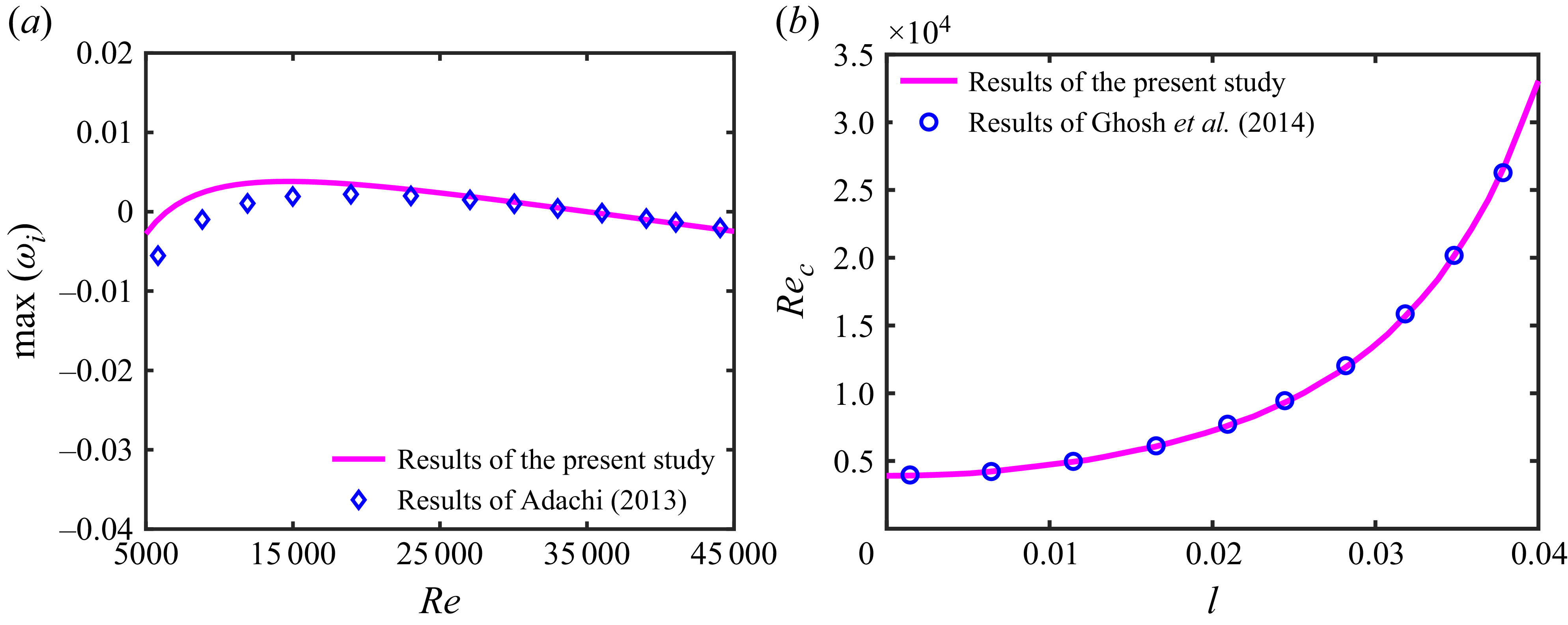


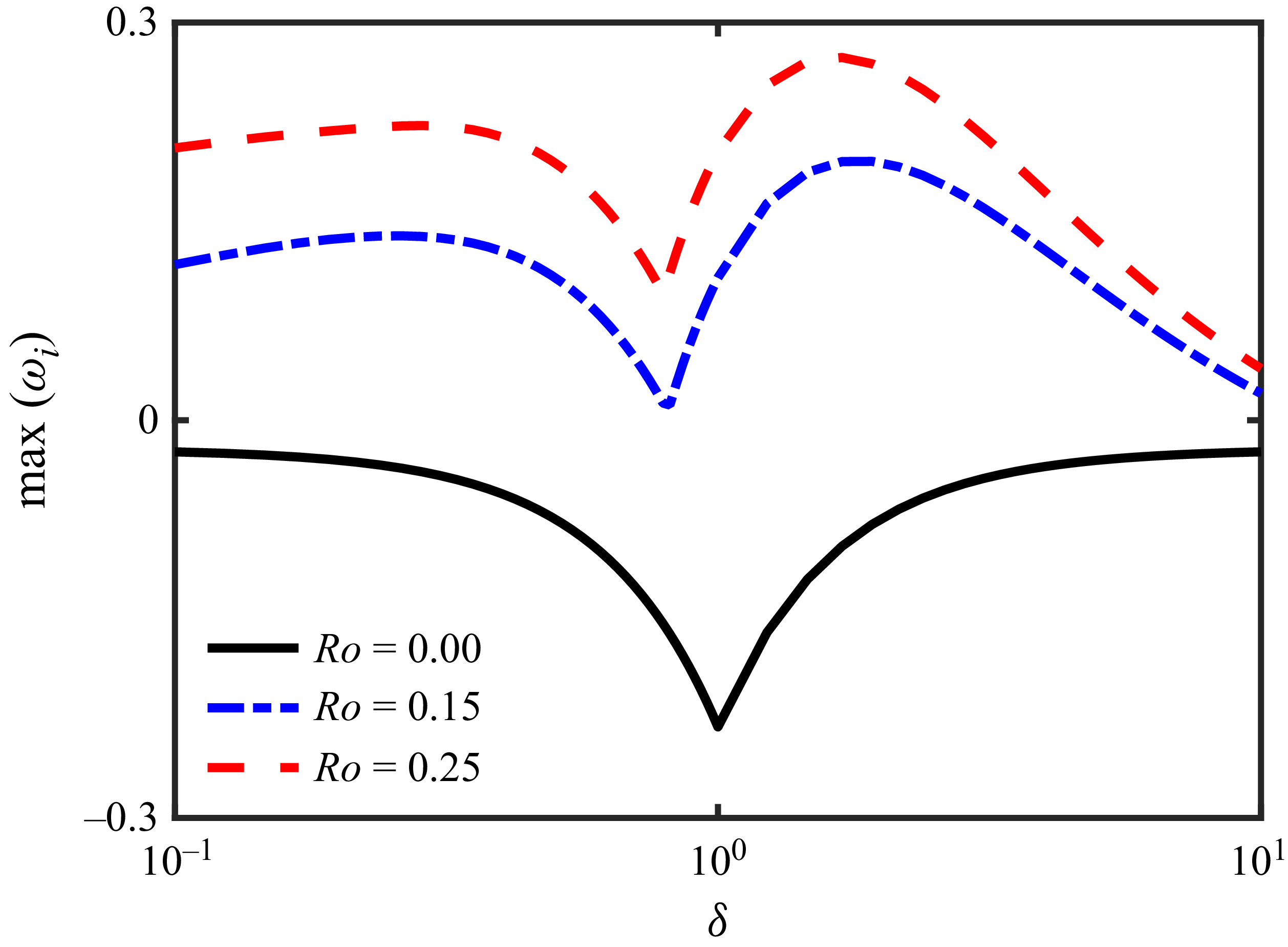


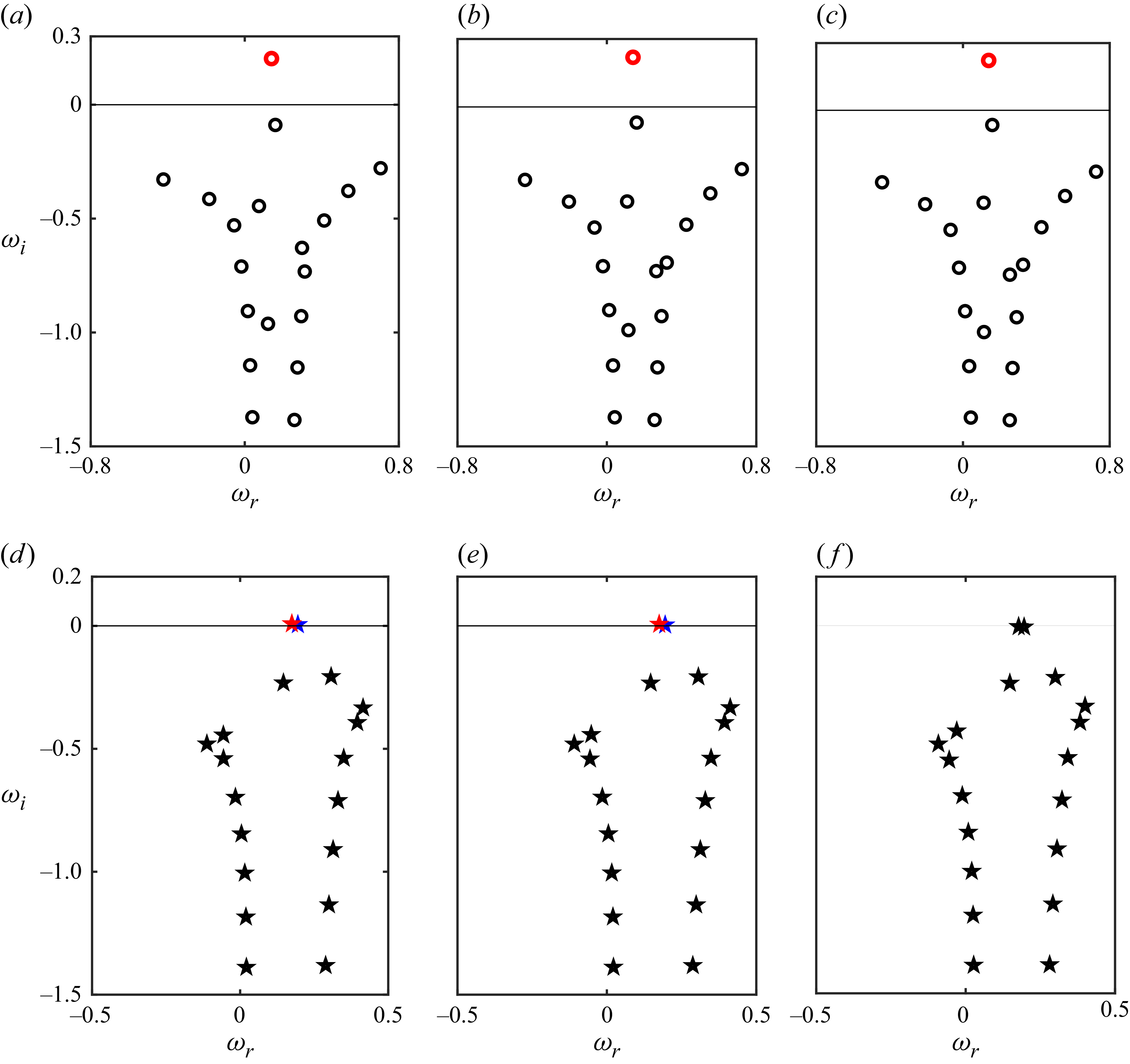


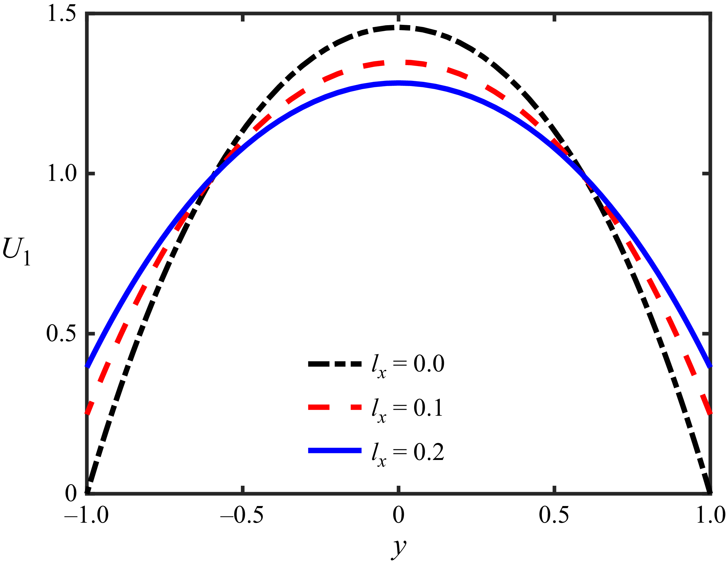


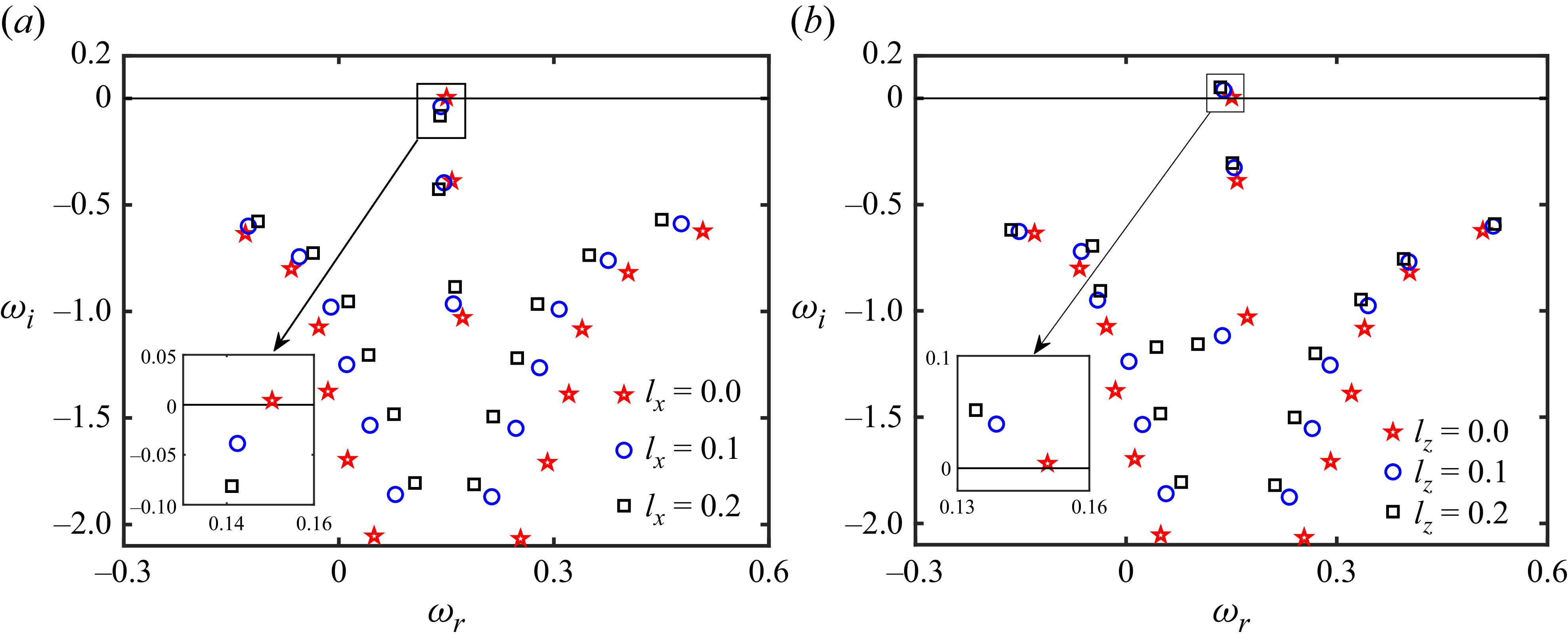


 Open access