


1. Introduction
The interaction between flames and finite-amplitude pressure waves, such as shock or blast waves, has attracted considerable research attention due to its critical role in diverse applications, ranging from propulsion systems to fire safety measures. In burners and combustion chambers, finite-amplitude acoustic oscillations at resonant frequencies often develop due to repeated reflections along the chamber boundaries (Jones & Thomas Reference Jones and Thomas1991; Dobashi, Hirano & Tsuruda Reference Dobashi, Hirano and Tsuruda1994). These finite-amplitude disturbances tend to distort and deform the flame inside the combustor. Contingent on the operating flow conditions (turbulence intensity, boundary conditions), the domain geometry and the reactivity of the fuel, this can lead to an increase in the local burning rates and can eventually transition the flame (deflagration wave) into a detonation front (Thomas, Bambrey & Brown Reference Thomas, Bambrey and Brown2001). Such transitions are vital in shaping the combustion dynamics of propulsion systems such as pulse detonation engines (Nikitin et al. Reference Nikitin, Dushin, Phylippov and Legros2009), which rely on detonations for efficient combustion and higher thrust. However, on the other hand, shock–flame interactions can also destabilise the flame and drive it towards extinction (Yoshida & Torikai Reference Yoshida and Torikai2024). This principle is utilised in large-scale fire extinguishing systems to fight wildfires and oil fires. They employ blast waves generated from explosives to blow off flames from the fuel source and extinguish them (Akhmetov, Lugovtsov & Tarasov Reference Akhmetov, Lugovtsov and Tarasov1980; Akhmetov Reference Akhmetov2001; Yoshida & Torikai Reference Yoshida and Torikai2024).
Traditionally, fundamental experimental studies on the interaction of flames with nonlinear pressure waves were performed inside a shock tube or a combustion chamber filled with a combustible mixture. Typically, the shock/blast front would be initiated at a chamber boundary after a characteristic time delay following the ignition of the mixture at a desired location inside the chamber. Pioneering work of Markstein (Reference Markstein1957) investigated the distortion of curved stoichiometric butane–air flames as a planar shock front swept across them from the unburnt side to the burnt side. He observed the emergence of an unburnt gas funnel that swiftly penetrated into the burnt side, inducing a reversal of the flame front and a rapid transition into fine turbulent structures. Recent studies from La Flèche (Reference La Flèche2018) reported similar observations following the interaction of a cellular flame front with a blast wave in a Hele-Shaw cell. The cellular flame was found to exhibit significant distortions and a reversal of the flame front as the blast wave swept through it from the unburnt side to the burnt side. These effects were attributed to the misalignment between the density and pressure gradient fields that contributes to local baroclinic vorticity production.
Further studies by Scarinci (Reference Scarinci1993) showed that the reaction rates were accelerated due to the enhanced vorticity production and that distortion of the flame front at larger time scales was contingent on the reactivity of the mixture. While a highly reactive mixture of acetylene and air was found to re-establish its initial flame shape owing to the increased reaction rates, which in turn caused a rise in viscous dissipation effects due to higher temperatures, a less reactive mixture like methane–air was found to retain its deformed shape for longer time scales. Numerical studies by Batley et al. (Reference Batley, McIntosh, Brindley and Falle1994, Reference Batley, McIntosh and Brindley1996) traced out the increment in the reaction rates against baroclinic vorticity production in a cylindrical laminar premixed flame following its interaction with a planar pressure wave. Thomas et al. (Reference Thomas, Bambrey and Brown2001) extended the above studies and demonstrated that multiple interactions of the flame with shocks can cause a substantial increase in the local temperature and pressure (accompanied by increased reaction rates) and can transition the flame into a detonation front.
While the aforementioned fundamental studies have significantly advanced our comprehension of flame interactions with nonlinear pressure waves, most studies focus on canonical configurations involving shocks generated in a confined chamber (which can be approximated to near-steady shock or unsteady shocks at low decay rates) and geometrically simple flame structures (planar/cylindrical/spherical flame front). Moving beyond canonical configurations, Chan et al. (Reference Chan, Giannuzzi, Kabir, Hargather and Doig2016) investigated shock–flame interactions in more practical burner settings. Their experiments employed non-premixed flames ranging from small Bunsen burners to large-scale ring burners. These flames were subjected to a transverse high-speed exhaust flow generated by a shock tube, which was characterised by a planar shock front followed by a high-momentum compressible vortex ring. Interestingly, the shock front itself caused minimal disruption to the flame. However, the subsequent induced flow was found to drive the flame to extinction. The study documented the minimal transverse velocity required to blow off the flame.
Building upon these studies, the current work explores the axial interaction between non-premixed jet flames and blast waves. The study employs a miniature blast-wave generator designed on the principle of high-voltage wire explosion (Oshima Reference Oshima, Chace and Moore1962). The technique involves imposing a high-voltage electrical impulse onto a thin metallic wire, causing it to vaporise instantaneously and form a dense metallic vapour cloud. The expansion of this high-temperature, high-pressure vapour column results in the formation of a blast wave. The initial blast front generated at the wire is cylindrical in nature, owing to the wire acting as a line source for the explosion. However, the blast rapidly transitions into an ellipsoidal form and eventually tends towards spherical symmetry at large propagation distances (Chiu, Lee & Knystautas Reference Chiu, Lee and Knystautas1977). The facility has been extensively used to study the secondary atomisation of liquid droplets at high Weber numbers (Sharma et al. Reference Sharma, Pratap Singh, Srinivas Rao, Kumar and Basu2021, Reference Sharma, Chandra, Kumar and Basu2023). Recent studies by Chandra et al. (Reference Chandra, Sharma, Basu and Kumar2023) validated the experimentally observed evolution of the generated blast wave against the theoretical blast-wave model developed by Bach & Lee (Reference Bach and Lee1970). It is to be noted that the generated blast wave is followed by an induced bulk flow, similar to that reported by Chan et al. (Reference Chan, Giannuzzi, Kabir, Hargather and Doig2016). Thus, the effective velocity/pressure profile exhibits two peaks, one corresponding to the blast front and the other corresponding to the subsequent induced flow. When this flow field is imposed on the jet flame, the large spatiotemporal flow-field gradients are expected to drastically alter its response dynamics compared with that observed in canonical shock/blast–flame interaction settings.
In addition to the expected distortion of the flame boundary following the interaction with the blast wave and the subsequent induced flow, the characteristic flickering instability of non-premixed jet flames is expected to alter under its influence. Flame flickering is a consequence of buoyancy-induced roll-up of toroidal vortices about the shear boundary between the hot product gases and the ambient air. The rolled-up vortices advect downstream and shed (detach from the feeding shear layer) upon reaching a critical circulation limit (Xia & Zhang Reference Xia and Zhang2018). This process of periodic vortex shedding induces a cyclical stretching of the flame tip, resulting in a visually perceived flickering behaviour. Our previous works (Pandey et al. Reference Pandey, Basu, Krishan and Gautham2021; Thirumalaikumaran, Vadlamudi & Basu Reference Thirumalaikumaran, Vadlamudi and Basu2022) investigating the flame dynamics of droplet diffusion flames subjected to external flows have demonstrated that the vortex roll-up rate in the shear boundary is aggravated in the presence of external flows and can even result in flame pinch-off events contingent on the operating conditions. Thus, the blast wave and subsequent induced flow, which impose large spatiotemporal velocity gradients, are expected to markedly alter the dynamics of flame flickering.
Building upon the arguments presented above, the present study aims to investigate the response dynamics of non-premixed jet flames following their axial interaction with a blast wave and the induced flow subsequent to it. The study classifies the response of the flame into distinct qualitative regimes across the parametric space of fuel-jet Reynolds number and blast-wave Mach number. Extending the theory of flame shedding developed by Xia & Zhang (Reference Xia and Zhang2018), the study proposes a simplified theoretical model to estimate shedding time scales following the interaction process.
2. Experimental set-up
2.1. Test facility
The experimental facility employed in the current work comprises a specially designed blast-wave generator and a fuel-jet nozzle built into it to facilitate the axial interaction between non-premixed jet flames and blast waves. The system is schematically depicted in figure 1(a). The blast-wave generator operates on the principle of high-voltage wire explosion and has been extensively used for shock/blast generation over the past few decades, particularly for droplet atomisation studies (Sharma et al. Reference Sharma, Pratap Singh, Srinivas Rao, Kumar and Basu2021; Chandra et al. Reference Chandra, Sharma, Basu and Kumar2023; Sharma et al. Reference Sharma, Chandra, Kumar and Basu2023). When a high-voltage electrical pulse of the order of a few kilovolts is imposed across a thin metallic wire, it results in rapid Joule heating of the wire, causing it to instantaneously melt and vaporise, thereby forming a dense column of metal vapour. The expansion of this vapour column generates the blast front (Oshima Reference Oshima, Chace and Moore1962). In the current system, a 2 kJ power pulse generator (Zeonics Systech, India Z/46/12) that houses a 5 μF capacitor is used to provide the high-voltage pulse across two electrodes that are connected through a thin metallic copper wire (35 SWG, length $L_{w}=75\,\rm mm$
). The charging voltage of the capacitor is varied between 4 and 7 kV, resulting in blast waves with reference Mach numbers (
$L_{w}=75\,\rm mm$
). The charging voltage of the capacitor is varied between 4 and 7 kV, resulting in blast waves with reference Mach numbers ( $M_{s,r} = ({u_{s}}/{c})_{ref}$
; Mach number measured at the reference location where the non-premixed flame is stabilised over the nozzle tip) spanning from 1.025 to 1.075. Here,
$M_{s,r} = ({u_{s}}/{c})_{ref}$
; Mach number measured at the reference location where the non-premixed flame is stabilised over the nozzle tip) spanning from 1.025 to 1.075. Here, $u_{s}$
is the speed of the blast front as measured at its instant of interaction with the non-premixed flame at the nozzle exit (detailed in § 2.2) and
$u_{s}$
is the speed of the blast front as measured at its instant of interaction with the non-premixed flame at the nozzle exit (detailed in § 2.2) and $c$
is the local speed of sound under ambient conditions (temperature of 298 K and pressure of 1 atm). A plot depicting the dependence of
$c$
is the local speed of sound under ambient conditions (temperature of 298 K and pressure of 1 atm). A plot depicting the dependence of $M_{s,r}$
on the capacitor charging voltage is presented in figure 2(a).
$M_{s,r}$
on the capacitor charging voltage is presented in figure 2(a).

Figure 1. (a) Schematic of the high-voltage electrode chamber that is used to generate blast waves. (b) Schematic of the experimental set-up and imaging facility used to visualise the interaction between non-premixed jet flames and blast waves.

Figure 2. (a) The variation of the reference blast-wave Mach number ( $M_{s,r}$
) at different capacitor charging voltages. (b) The variation of the flame height of the non-premixed jet flame across the parametric space of fuel-jet Reynolds numbers. (c) Response of the non-premixed flame to the blast front and the induced flow that trails behind it.
$M_{s,r}$
) at different capacitor charging voltages. (b) The variation of the flame height of the non-premixed jet flame across the parametric space of fuel-jet Reynolds numbers. (c) Response of the non-premixed flame to the blast front and the induced flow that trails behind it.
A fuel-jet nozzle tube, with an inner diameter ( $d$
) of 2 mm, is centrally positioned with respect to the electrode base plate. This base plate forms the section of the electrode chamber over which the electrodes are connected with the thin copper wire. As depicted in figure 1(a), the nozzle tube, positioned equidistantly relative to both electrodes, conveys methane gas. A precise mass flow controller (Bronkhorst Flexi Flow Compact, capacity: 0–1.6 SLPM) regulates the methane feed. The nozzle stabilises a non-premixed jet flame at its exit, located 264 mm above the base plate. In the current study, the fuel-jet velocity (
$d$
) of 2 mm, is centrally positioned with respect to the electrode base plate. This base plate forms the section of the electrode chamber over which the electrodes are connected with the thin copper wire. As depicted in figure 1(a), the nozzle tube, positioned equidistantly relative to both electrodes, conveys methane gas. A precise mass flow controller (Bronkhorst Flexi Flow Compact, capacity: 0–1.6 SLPM) regulates the methane feed. The nozzle stabilises a non-premixed jet flame at its exit, located 264 mm above the base plate. In the current study, the fuel-jet velocity ( $v_{j}$
) is varied between 1 and 3 ms–1 in steps of 0.5 ms–1, varying the fuel-jet Reynolds number (
$v_{j}$
) is varied between 1 and 3 ms–1 in steps of 0.5 ms–1, varying the fuel-jet Reynolds number ( $Re = {v_{f}d}/{\nu _{f}}$
) from 267 to 800, in steps of 133. The flame height (estimation presented in § 2.2) was found to increase with an increase in the fuel-jet Reynolds number, and their dependence is depicted in figure 2(b).
$Re = {v_{f}d}/{\nu _{f}}$
) from 267 to 800, in steps of 133. The flame height (estimation presented in § 2.2) was found to increase with an increase in the fuel-jet Reynolds number, and their dependence is depicted in figure 2(b).
During the experimental runs, the fuel jet is set to a desired Reynolds number, and the non-premixed jet flame is stabilised at the nozzle exit using a pilot flame. Simultaneously, the 5 μF capacitor is charged to a required voltage level contingent on the operating $M_{s,r}$
. Once charged, the charging circuit is cut off. The discharge circuit running through the electrodes and the thin copper wire is triggered upon receiving a TTL pulse from a digital delay generator (BNC 757) that synchronises the blast-generation process with the imaging systems (see figure 1
b).
$M_{s,r}$
. Once charged, the charging circuit is cut off. The discharge circuit running through the electrodes and the thin copper wire is triggered upon receiving a TTL pulse from a digital delay generator (BNC 757) that synchronises the blast-generation process with the imaging systems (see figure 1
b).
Figure 2(c) illustrates the initial phase of the interaction between the blast wave and the non-premixed jet flame. The blast wave imposes a characteristic flow-field profile on the jet flame marked by a sharp discontinuity, followed by a decaying profile that drops to subambient levels within a characteristic time period. Nonetheless, an induced bulk flow trails behind the blast front, introducing an additional flow component that modifies the dynamics of the jet flame at extended time scales. These observations are elaborated upon extensively in §§ 2.3 and 3.1. The interaction process was investigated using a combination of schlieren flow visualisation and OH* chemiluminescence imaging. The schlieren set-up utilised a pair of parabolic concave mirrors with a focal length of 1500 mm. A high-speed, non-coherent pulse diode laser (Cavitar Cavilux smart UHS, 400 W), emitting at a wavelength of 640 nm, served as the light source (depicted in figure 1
b). Schlieren visualisation was performed at 40 000 frames per second using a high-speed Star SA5 Photron Camera. Simultaneous OH* chemiluminescence imaging was performed using a LaVision SA5 high-speed camera, coupling it with a high-speed intensifier (LaVision HS-IRO, IV Generation), a UV lens (Nikon Rayfact PF10445MF) and an OH* bandpass filter ( $\sim$
310 nm). The acquisition rate was set to 10 000 frames per second for OH* chemiluminescence imaging. The spatial resolutions for schlieren visualisation and OH* chemiluminescence imaging were set to 5.012 and 3.430 px mm−1, respectively.
$\sim$
310 nm). The acquisition rate was set to 10 000 frames per second for OH* chemiluminescence imaging. The spatial resolutions for schlieren visualisation and OH* chemiluminescence imaging were set to 5.012 and 3.430 px mm−1, respectively.
2.2. Data processing
The OH* chemiluminescence images of the flame were analysed using ImageJ software. The Otsu thresholding technique, integrated within ImageJ, was employed to identify the flame boundary. This method effectively segregates the image pixels as foreground (flame) and background based on an intensity threshold ( $I_f$
). This threshold is determined by minimising the variance within each category (foreground and background), effectively maximising the variance between them. Pixels with intensities exceeding
$I_f$
). This threshold is determined by minimising the variance within each category (foreground and background), effectively maximising the variance between them. Pixels with intensities exceeding $I_f$
are assigned a binary value of 1 (designated as flame), while those falling below the threshold are assigned a value of 0 (designated as background). The technique is explained in detail in Supplementary § S1. The resulting contiguous region of pixels with a value of 1 subsequently demarcates the flame perimeter.
$I_f$
are assigned a binary value of 1 (designated as flame), while those falling below the threshold are assigned a value of 0 (designated as background). The technique is explained in detail in Supplementary § S1. The resulting contiguous region of pixels with a value of 1 subsequently demarcates the flame perimeter.
Following blast-wave interaction, the spatiotemporal response dynamics of the flame base and flame tip were tracked individually. Flame height was estimated as the vertical distance between the flame tip and the flame base. The OH* chemiluminescence signal, indicative of the flame’s overall heat release rate, was obtained by integrating the pixel intensities within the delineated flame boundary in the original image. To ensure reliable data, all flame descriptors presented hereafter (flame tip and base positions, height and OH* chemiluminescence signal) represent the average of at least three independent experimental trials. The error bars presented in the plots of subsequent sections correspond to the standard deviation of these trials.

Figure 3. A comparison between the experimentally measured temporal evolution of the blast wave at charging voltages of 4 and 7 kV against the analytical blast-wave model proposed by Bach & Lee (Reference Bach and Lee1970) is presented. The trends observed in the (a) blast-wave radius and (b) Mach number are compared.
Schlieren imaging provided a means to visualise the evolution of the blast wave. By spatially tracking the position of the blast wave (along the axis of the fuel jet) with respect to time in schlieren images, a time-dependent variation of the blast-wave radius ( $R_s$
) was obtained. The data were then used to estimate the velocity of the blast front (
$R_s$
) was obtained. The data were then used to estimate the velocity of the blast front ( $u_{s}$
) and, subsequently, the blast-wave Mach number (
$u_{s}$
) and, subsequently, the blast-wave Mach number ( $M_{s}$
).
$M_{s}$
).

Figure 4. The theoretical flow-field profiles imposed by the blast wave at the nozzle exit location. The profiles correspond to charging voltages of 4 and 7 kV. The blast-imposed (a) velocity and (b) pressure fields are presented.
2.3. Characterisation of the flow field imposed by the blast wave
Owing to the cylindrical geometry of the exploding wire, the initial blast front is expected to exhibit a cylindrical form. Studies suggest that these cylindrical blast fronts initially transition to ellipsoidal forms and ultimately evolve into spherical fronts in the far field. However, at blast propagation distances ( $R_{s}$
) of the order of the characteristic length of the exploding wire (
$R_{s}$
) of the order of the characteristic length of the exploding wire ( $L_{w}$
), the ellipsoidal nature of the blast front is found to be retained (Chiu et al. Reference Chiu, Lee and Knystautas1977). Our experimental data on the temporal evolution of the blast-wave radius and Mach number are also found to align more favourably with the theoretical model (Bach & Lee Reference Bach and Lee1970; detailed in Supplementary § S2) of an expanding cylindrical blast wave compared with a spherical blast wave (presented in Supplementary § S3). This consistency suggests that during the blast–flame interaction process, the cylindrical nature of the blast wave is likely preserved in the immediate vicinity of the fuel-jet axis. Moreover, the observed ratio of the blast-wave radius (during the interaction with the jet flame) to the characteristic wire length (
$L_{w}$
), the ellipsoidal nature of the blast front is found to be retained (Chiu et al. Reference Chiu, Lee and Knystautas1977). Our experimental data on the temporal evolution of the blast-wave radius and Mach number are also found to align more favourably with the theoretical model (Bach & Lee Reference Bach and Lee1970; detailed in Supplementary § S2) of an expanding cylindrical blast wave compared with a spherical blast wave (presented in Supplementary § S3). This consistency suggests that during the blast–flame interaction process, the cylindrical nature of the blast wave is likely preserved in the immediate vicinity of the fuel-jet axis. Moreover, the observed ratio of the blast-wave radius (during the interaction with the jet flame) to the characteristic wire length ( $R_{s}/L_{w}$
) of approximately 3.5 in our experiments suggests that
$R_{s}/L_{w}$
) of approximately 3.5 in our experiments suggests that $R_{s}$
and
$R_{s}$
and $L_{w}$
are comparable. This further reinforces the notion of a cylindrical blast front interacting with the jet flame (Chiu et al. Reference Chiu, Lee and Knystautas1977). Details illustrating the implementation of the theoretical blast-wave model for the present experimental configuration are presented in Supplementary § S3.
$L_{w}$
are comparable. This further reinforces the notion of a cylindrical blast front interacting with the jet flame (Chiu et al. Reference Chiu, Lee and Knystautas1977). Details illustrating the implementation of the theoretical blast-wave model for the present experimental configuration are presented in Supplementary § S3.
It is to be noted that the theoretical blast model (Bach & Lee Reference Bach and Lee1970) relies on an assumed power-law profile for the density field behind the blast front and estimates the velocity and pressure fields using conservation equations. Additionally, the model assumes that the total mass and energy contained within the blast front remain constant during the evolution process (detailed in Supplementary § S2), effectively neglecting entrainment from the surroundings, which is anticipated when the blast-imposed static pressure field drops below ambient levels. The theoretical estimates of the velocity and pressure fields imposed by a cylindrical blast wave at the nozzle exit (radial distance of 264 mm from the source of the explosion) are plotted in figures 4(a) and 4(b), respectively. The blast wave is found to reach the nozzle exit location after a time of $t_{i}$
from the time of the explosion (
$t_{i}$
from the time of the explosion ( $t=0$
). Thus, the blast wave interacts with the non-premixed jet flame (that is stabilised at the nozzle exit) beyond
$t=0$
). Thus, the blast wave interacts with the non-premixed jet flame (that is stabilised at the nozzle exit) beyond $t_{i}$
. The blast-imposed pressure field attains a peak (
$t_{i}$
. The blast-imposed pressure field attains a peak ( $p_{p}$
) at the instant of interaction (
$p_{p}$
) at the instant of interaction ( $t_{i}$
) and is followed by a decaying profile that attains subambient levels beyond the time of
$t_{i}$
) and is followed by a decaying profile that attains subambient levels beyond the time of $t_{s,p}$
(figure 4
b). A similar trend is observed for the blast-induced velocity field (figure 4
a), wherein the velocity reaches a peak value (
$t_{s,p}$
(figure 4
b). A similar trend is observed for the blast-induced velocity field (figure 4
a), wherein the velocity reaches a peak value ( $v_p$
) at
$v_p$
) at $t_{i}$
and then decays to subambient levels beyond
$t_{i}$
and then decays to subambient levels beyond $t_{s,v}$
. It is important to note that beyond
$t_{s,v}$
. It is important to note that beyond $t_{s,p}$
, entrainment from the surrounding medium is anticipated, and this renders the analytical solution inaccurate in predicting the flow field.
$t_{s,p}$
, entrainment from the surrounding medium is anticipated, and this renders the analytical solution inaccurate in predicting the flow field.
Alongside the blast wave, the flame responds to the delayed, induced bulk flow that follows it. Induced flow following the blast front is a characteristic feature of expanding shock/blast waves and has been reported earlier as ‘blast wind’ by Chan et al. (Reference Chan, Giannuzzi, Kabir, Hargather and Doig2016). Due to the limitations in experimentally measuring the detailed velocity profile of the induced flow, we could only estimate its characteristic velocity scale based on the flame’s response following the interaction with it (detailed in the following section).

Figure 5. The response of a non-premixed jet flame to blast waves and the subsequent induced flow, categorised by two distinct time scales: the initial flame response at times lower than $t_{s,p}$
(a), and the response to the induced flow with subregimes of reattachment (Type-1 and Type-2) (b,c) and extinction (Type-1 and Type-2) (d,e) at times greater than
$t_{s,p}$
(a), and the response to the induced flow with subregimes of reattachment (Type-1 and Type-2) (b,c) and extinction (Type-1 and Type-2) (d,e) at times greater than $t_{s,p}$
. Supplementary movies 1–4 correspond to the depicted subregimes in (b–e), respectively. The yellow dotted lines represent the location of the nozzle tip.
$t_{s,p}$
. Supplementary movies 1–4 correspond to the depicted subregimes in (b–e), respectively. The yellow dotted lines represent the location of the nozzle tip.
3. Results and discussion
3.1. Global observations
As the blast wave traverses through the non-premixed jet flame, it imposes a characteristic flow field on the jet flame, described by a sharp peak followed by a decaying phase, as outlined in the previous section (figure 4
a; $t_{i}\lt t\lt t_{s,p}$
). Additionally, the induced flow interacts with the jet flame after a characteristic time delay following the passage of the blast front. Figure 5 illustrates the flame’s response to the blast front and the subsequent induced bulk flow. The response at time scales lower than
$t_{i}\lt t\lt t_{s,p}$
). Additionally, the induced flow interacts with the jet flame after a characteristic time delay following the passage of the blast front. Figure 5 illustrates the flame’s response to the blast front and the subsequent induced bulk flow. The response at time scales lower than $t_{s,p}$
is presented in figure 5(a), while figure 5(b–e) depicts the response at time scales beyond
$t_{s,p}$
is presented in figure 5(a), while figure 5(b–e) depicts the response at time scales beyond $t_{s,p}$
.
$t_{s,p}$
.
Observations reveal that the flame exhibits minimal response to the initial blast front and the decaying flow field behind it (figure 5
a). At time scales below $t_{s,p}$
, the flame displays only a jittery motion. However, the flame base is found to lift off from the nozzle exit at
$t_{s,p}$
, the flame displays only a jittery motion. However, the flame base is found to lift off from the nozzle exit at $t = t_{0}$
, where
$t = t_{0}$
, where $t_{0}\gt t_{s,p}$
(figure 5
b–e; first frame). This response corresponds to the induced flow following the blast wave. It is interesting to note that the flame base lift-off rate, at the instant of lift-off,
$t_{0}\gt t_{s,p}$
(figure 5
b–e; first frame). This response corresponds to the induced flow following the blast wave. It is interesting to note that the flame base lift-off rate, at the instant of lift-off, $t_{0}$
, remains at a near-constant value across the investigated range of fuel-jet Reynolds numbers (figure 6
b). The plot also reveals a positive correlation between the observed flame base lift-off rate at
$t_{0}$
, remains at a near-constant value across the investigated range of fuel-jet Reynolds numbers (figure 6
b). The plot also reveals a positive correlation between the observed flame base lift-off rate at $t_{0}$
and the strength of the incident blast wave. Anticipating a higher velocity scale for the induced flow at higher Mach numbers, the observed trend in figure 6(b) can be attributed to the increased induced flow velocities at higher Mach numbers.
$t_{0}$
and the strength of the incident blast wave. Anticipating a higher velocity scale for the induced flow at higher Mach numbers, the observed trend in figure 6(b) can be attributed to the increased induced flow velocities at higher Mach numbers.

Figure 6. (a) Schematic depicting the lift-off of the jet flame following the interaction with the induced flow. (b) Plot illustrating the flame base lift-off rate at the instant of interaction with the induced flow ( $t_{0}$
) across the parametric space of fuel-jet Reynolds number.
$t_{0}$
) across the parametric space of fuel-jet Reynolds number.
Therefore, we propose the following hypothesis: before $t_{0}$
, the non-premixed jet flame remained stabilised on the nozzle rim within a narrow mixing layer between the fuel jet and the surrounding ambient air, wherein heat losses locally balance out the energy generated at the flame front (Li, Liu & Wang Reference Li, Liu and Wang2022). Upon encountering the induced flow, this local energy balance within the mixing layer is disrupted, and the flame’s stoichiometric plane tends to convect with the induced flow (figure 6
a). Thus, the estimated flame base lift-off rate at the instant of lift-off (
$t_{0}$
, the non-premixed jet flame remained stabilised on the nozzle rim within a narrow mixing layer between the fuel jet and the surrounding ambient air, wherein heat losses locally balance out the energy generated at the flame front (Li, Liu & Wang Reference Li, Liu and Wang2022). Upon encountering the induced flow, this local energy balance within the mixing layer is disrupted, and the flame’s stoichiometric plane tends to convect with the induced flow (figure 6
a). Thus, the estimated flame base lift-off rate at the instant of lift-off ( $t_{0}$
) can be approximated as the velocity scale of the induced flow that interacts with it. The variation of these induced flow velocity scales across the parametric space of
$t_{0}$
) can be approximated as the velocity scale of the induced flow that interacts with it. The variation of these induced flow velocity scales across the parametric space of $M_{s,r}$
is plotted in figure 7(a):
$M_{s,r}$
is plotted in figure 7(a):
 \begin{gather} v_{in} \sim \left ( \frac {{\rm d}x_{b}}{{\rm d}t} \right )_{t_{0}}. \end{gather}
Following the flame base lift-off, the flame is found to exhibit two global response behaviours: reattachment and extinction. In the reattachment regimes (figure 5
b,c), the flame base is found to attain a maximum lift-off height of $h_{b,lft}$
in a period of
$h_{b,lft}$
in a period of $t_{b,lft}$
, and then reattach back at the nozzle rim in a characteristic time period of
$t_{b,lft}$
, and then reattach back at the nozzle rim in a characteristic time period of $t_{b,ra}$
. However, contingent on the operating fuel-jet Reynolds number and the strength of the incident blast wave, the flame-tip response dynamics varies. In the reattachment-1 (Type-1) regime, the flame tip exhibits mild distortion and stretching owing to the interaction with the induced flow (figure 5
b). However, in the reattachment-2 (Type-2) regime (figure 5
c), the flame tip is found to exhibit a pinch-off event following neck formation at the flame tip. Further details and trends observed in the response dynamics of the flame base and flame tip in the reattachment regimes are detailed in § 3.2. It is to be noted that as the flame base lifts off following the interaction with the induced flow, ambient air is entrained into the fuel-jet stream (figure 6
a). As the fuel and coaxial air streams mix into each other, the lifted flame is expected to attain an edge-flame configuration at the flame base (Buckmaster Reference Buckmaster2002; Vadlamudi, Aravind & Basu Reference Vadlamudi, Aravind and Basu2023). Such flame structures can propagate upstream with a characteristic propagation velocity. Given that the lifted flame reattaches to the nozzle rim within a time period of
$t_{b,ra}$
. However, contingent on the operating fuel-jet Reynolds number and the strength of the incident blast wave, the flame-tip response dynamics varies. In the reattachment-1 (Type-1) regime, the flame tip exhibits mild distortion and stretching owing to the interaction with the induced flow (figure 5
b). However, in the reattachment-2 (Type-2) regime (figure 5
c), the flame tip is found to exhibit a pinch-off event following neck formation at the flame tip. Further details and trends observed in the response dynamics of the flame base and flame tip in the reattachment regimes are detailed in § 3.2. It is to be noted that as the flame base lifts off following the interaction with the induced flow, ambient air is entrained into the fuel-jet stream (figure 6
a). As the fuel and coaxial air streams mix into each other, the lifted flame is expected to attain an edge-flame configuration at the flame base (Buckmaster Reference Buckmaster2002; Vadlamudi, Aravind & Basu Reference Vadlamudi, Aravind and Basu2023). Such flame structures can propagate upstream with a characteristic propagation velocity. Given that the lifted flame reattaches to the nozzle rim within a time period of $t_{b,ra}$
, it can be hypothesised that at time scales beyond
$t_{b,ra}$
, it can be hypothesised that at time scales beyond $t_{b,lft}$
(at
$t_{b,lft}$
(at $t_{b,lft}$
, the flame base attains maximum lift-off height), the induced flow field decays to velocities lower than the characteristic propagation velocity of the edge-flame structure. As a result, the flame reattaches to the nozzle rim. Thus, based on the estimated time scale (
$t_{b,lft}$
, the flame base attains maximum lift-off height), the induced flow field decays to velocities lower than the characteristic propagation velocity of the edge-flame structure. As a result, the flame reattaches to the nozzle rim. Thus, based on the estimated time scale ( $\sim O(t_{b,lft})$
) and velocity scale (
$\sim O(t_{b,lft})$
) and velocity scale ( $\sim ({{\rm d}x_{b}}/{{\rm d}t})_{t_{0}}$
) of the induced flow, a schematic of the anticipated induced flow profile is sketched in figure 7(b). It is to be noted that the decay time scale of the induced flow (
$\sim ({{\rm d}x_{b}}/{{\rm d}t})_{t_{0}}$
) of the induced flow, a schematic of the anticipated induced flow profile is sketched in figure 7(b). It is to be noted that the decay time scale of the induced flow ( $\sim O(t_{b,lft})$
) is at least an order of magnitude higher in comparison with the decay time scales associated with the blast wave (
$\sim O(t_{b,lft})$
) is at least an order of magnitude higher in comparison with the decay time scales associated with the blast wave ( $t_{s,v}$
and
$t_{s,v}$
and $t_{s,p}$
).
$t_{s,p}$
).

Figure 7. (a) Variation of the estimated induced flow velocity scale ( $v_{in}$
) across
$v_{in}$
) across $M_{s,r}$
. (b) Schematic depicting the velocity profile at the nozzle exit location imposed by the blast wave and the induced flow following it.
$M_{s,r}$
. (b) Schematic depicting the velocity profile at the nozzle exit location imposed by the blast wave and the induced flow following it.
Another global flame response behaviour that was observed was flame extinction. In this regime, the flame base, which lifts off following the interaction with the induced flow, would continue its lift-off without reaching a maximum. This results in an eventual extinction, as illustrated in figure 5(d,e). Similar to the reattachment regimes, Type-1 and Type-2 response behaviours were also noted in the extinction regimes. In the Type-1 subregime, flame-tip distortions are minimal (see figure 5 d), while in the Type-2 subregime, a notable flame necking event occurs (see figure 5 e). However, unlike the reattachment-2 regime, flame pinch-off was not consistently observed throughout the extinction-2 regime, despite neck formation. These trends are further discussed in detail in § 3.3. A schematic illustrating the reattachment and extinction flame behaviours (Type-1 and Type-2) is presented in Supplementary § S5.

Figure 8. (a) Schematic depicting the density gradient field around the flame boundary and the pressure gradient field associated with the blast wave prior to their interaction. (b) Schematic depicting the cusp formation and reversal of the flame base interface following the interaction with the blast wave.
Another interesting observation was the reversal of the flame shape at the flame base following the interaction process, a phenomenon consistently observed across both the reattachment and extinction regimes. As the blast wave and the induced flow subsequent to it traverse through the non-premixed jet flame, it imposes a pressure gradient at the flame location oriented upstream along the jet axis (figure 8 a). The density boundary at the interface of the hot product gases and the ambient air has a component of the density gradient field directly radially outward, orthogonal to the fuel-jet axis. This misalignment between the density and pressure gradient fields generates vorticity at the interface, leading to deformation. To understand the mechanism behind this deformation, let us formulate the vorticity transport equation at the interface of the hot product gases and the ambient air:
 \begin{gather} \frac {{\rm D}\omega }{{\rm D}t}=\left (\omega .\nabla \right )u-\ \omega \left (\nabla .u\right )+ \frac {1}{\rho ^2}\left (\nabla \rho \times \nabla p\right )+\frac {\rho _a}{\rho ^2}\left (\nabla \rho \times g\right )+\ \nu \nabla ^2\omega .\end{gather}
In the above equation, $\omega$
represents vorticity,
$\omega$
represents vorticity, $\rho$
denotes density,
$\rho$
denotes density, $p$
signifies pressure,
$p$
signifies pressure, $u$
is the velocity,
$u$
is the velocity, $\nu$
is the kinematic viscosity and
$\nu$
is the kinematic viscosity and $\rho _{a}$
is the density of ambient air. Since the flow is incompressible, axisymmetric and devoid of swirl, the first and second terms on the right-hand side of the equation are zero. Due to the component of the density gradient field oriented orthogonal to the blast-imposed pressure gradient field (figure 8
a), the third term becomes negative, leading to vorticity production along the interface. This causes the interface to deform, which, at longer time scales, evolves into a cusp at the flame base, eventually causing a reversal of the flame front along the centreline (figure 8
b). Similar observations were reported earlier by Markstein (Reference Markstein1957), Vadlamudi et al. (Reference Vadlamudi, Aravind, Rao and Basu2024) and La Flèche (Reference La Flèche2018), where the concavity of the flame boundary was reversed as a shock wave passed from the unburnt side to the burnt side, resembling the scenario discussed here. These effects are particularly pronounced at higher blast strengths, as the imposed pressure gradients increase with increasing Mach number. The variation of the peak blast-imposed pressure gradients against
$\rho _{a}$
is the density of ambient air. Since the flow is incompressible, axisymmetric and devoid of swirl, the first and second terms on the right-hand side of the equation are zero. Due to the component of the density gradient field oriented orthogonal to the blast-imposed pressure gradient field (figure 8
a), the third term becomes negative, leading to vorticity production along the interface. This causes the interface to deform, which, at longer time scales, evolves into a cusp at the flame base, eventually causing a reversal of the flame front along the centreline (figure 8
b). Similar observations were reported earlier by Markstein (Reference Markstein1957), Vadlamudi et al. (Reference Vadlamudi, Aravind, Rao and Basu2024) and La Flèche (Reference La Flèche2018), where the concavity of the flame boundary was reversed as a shock wave passed from the unburnt side to the burnt side, resembling the scenario discussed here. These effects are particularly pronounced at higher blast strengths, as the imposed pressure gradients increase with increasing Mach number. The variation of the peak blast-imposed pressure gradients against $M_{s,r}$
is presented in Supplementary § S6(a).
$M_{s,r}$
is presented in Supplementary § S6(a).

Figure 9. Regime map illustrating the diverse flame response behaviours to the blast wave and the ensuing induced flow, spanning the parametric space of fuel-jet Reynolds number and the incident blast-wave Mach number.
It should be noted that the fourth and fifth terms on the right-hand side of (3.2) are significantly smaller (in magnitude) compared with the third term at the instant of interaction. This is because the pressure gradient associated with the blast front dominates over the contributions from body forces (fourth term) and viscous dissipation effects (fifth term). Supplementary figure S6(b) plots the temporal evolution of the ratio of $\nabla p$
and
$\nabla p$
and $\rho _{a} g$
at the flame base location (ratio of the third and fourth terms on the right-hand side of (3.2)). The plots illustrate that the influence of the blast-imposed pressure gradients is limited to a very short span of time (
$\rho _{a} g$
at the flame base location (ratio of the third and fourth terms on the right-hand side of (3.2)). The plots illustrate that the influence of the blast-imposed pressure gradients is limited to a very short span of time ( ${\sim} 1 \space \rm m\, s$
). However, as demonstrated by Vadlamudi et al. (Reference Vadlamudi, Aravind, Rao and Basu2024), the response of the flame to Richtmyer–Meshkov (RM) instability (cusp formation and flame-front reversal) persists beyond this time scale (particularly when the Mach number is less than 1.1, which corresponds to the current scenario) and is evident from the plots in figure 5(e) (t = 2.55 ms). For a more detailed understanding of the flame-front evolution over extended time periods following RM instability, the reader is referred to the work of Attal & Ramaprabhu (Reference Attal and Ramaprabhu2015).
${\sim} 1 \space \rm m\, s$
). However, as demonstrated by Vadlamudi et al. (Reference Vadlamudi, Aravind, Rao and Basu2024), the response of the flame to Richtmyer–Meshkov (RM) instability (cusp formation and flame-front reversal) persists beyond this time scale (particularly when the Mach number is less than 1.1, which corresponds to the current scenario) and is evident from the plots in figure 5(e) (t = 2.55 ms). For a more detailed understanding of the flame-front evolution over extended time periods following RM instability, the reader is referred to the work of Attal & Ramaprabhu (Reference Attal and Ramaprabhu2015).
Figure 9 illustrates the parametric space of fuel-jet Reynolds numbers and reference blast-wave Mach numbers ( $M_{s,r}$
) over which different flame response regimes were observed. Reducing the fuel-jet Reynolds number and increasing the blast strength were found to make the flame vulnerable to extinction. Reattachment-1 response was restricted to the lowest blast strength (
$M_{s,r}$
) over which different flame response regimes were observed. Reducing the fuel-jet Reynolds number and increasing the blast strength were found to make the flame vulnerable to extinction. Reattachment-1 response was restricted to the lowest blast strength ( $M_{s,r}=1.025$
) across the entire range of
$M_{s,r}=1.025$
) across the entire range of $Re$
. The reattachment-2 regime was noted for
$Re$
. The reattachment-2 regime was noted for $Re\geqslant 400$
and
$Re\geqslant 400$
and $Re\geqslant 667$
at blast-wave Mach numbers of 1.040 and 1.060, respectively. The extinction-1 regime was dominant in shorter flames and persisted upto the Reynolds numbers of 267, 534 and 400 at blast-wave Mach numbers (
$Re\geqslant 667$
at blast-wave Mach numbers of 1.040 and 1.060, respectively. The extinction-1 regime was dominant in shorter flames and persisted upto the Reynolds numbers of 267, 534 and 400 at blast-wave Mach numbers ( $M_{s,r}$
) of 1.040, 1.060 and 1.075, respectively. The extinction-2 subregime was observed at the highest blast strength (
$M_{s,r}$
) of 1.040, 1.060 and 1.075, respectively. The extinction-2 subregime was observed at the highest blast strength ( $M_{s,r}=1.075$
) for
$M_{s,r}=1.075$
) for $Re\geqslant 534$
. Sections 3.2 and 3.3 detail the trends observed in the reattachment and extinction regimes, respectively.
$Re\geqslant 534$
. Sections 3.2 and 3.3 detail the trends observed in the reattachment and extinction regimes, respectively.
3.2. Reattachment response regimes
Figure 10(a,b) depicts the flame response in reattachment-1 and reattachment-2 subregimes. The plots track the temporal evolution of the flame base and flame tip alongside the OH* chemiluminescence signal of the flame. As explained earlier in § 3.1, the flame base tends to lift off from the nozzle rim following the interaction with the induced flow.
The lifted flame attains a maximum lift-off height of $h_{b,lft}$
in a time period of
$h_{b,lft}$
in a time period of $t_{b,lft}$
(figure 10
a,b), both of which are found to increase with an increase in the fuel-jet Reynolds number (
$t_{b,lft}$
(figure 10
a,b), both of which are found to increase with an increase in the fuel-jet Reynolds number ( $Re$
) and the induced flow velocity (
$Re$
) and the induced flow velocity ( $v_{in}$
), as illustrated in figure 11(a,b). In the plots,
$v_{in}$
), as illustrated in figure 11(a,b). In the plots, $h_{b,lft}$
and
$h_{b,lft}$
and $t_{b,lft}$
are non-dimensionalised with
$t_{b,lft}$
are non-dimensionalised with $d$
(diameter of the nozzle tube) and
$d$
(diameter of the nozzle tube) and $t_{diff}$
, respectively. Here
$t_{diff}$
, respectively. Here $t_{diff}$
is the diffusion time scale associated with methane (fuel) diffusing into the ambient air over a length scale of
$t_{diff}$
is the diffusion time scale associated with methane (fuel) diffusing into the ambient air over a length scale of $d$
(
$d$
( $t_{diff} = d^{2}/D$
, where D is the molecular diffusion coefficient (Langenberg et al. Reference Langenberg, Carstens, Hupperich, Schweighoefer and Schurath2020)).
$t_{diff} = d^{2}/D$
, where D is the molecular diffusion coefficient (Langenberg et al. Reference Langenberg, Carstens, Hupperich, Schweighoefer and Schurath2020)).

Figure 10. The temporal response of the flame base (blue) and the flame tip (red) alongside the OH* chemiluminescence signal of the jet flame as it interacts with the blast wave and the subsequent induced flow: (a) reattachment-1 and (b) reattachment -2 subregimes. In the plots, the spatial position ( $x$
) is normalised with the nozzle diameter (d) and time is normalised with the time scale associated with the diffusion of methane into ambient air over a characteristic length scale of
$x$
) is normalised with the nozzle diameter (d) and time is normalised with the time scale associated with the diffusion of methane into ambient air over a characteristic length scale of $d$
(
$d$
( $t_{diff}$
). Additionally, the OH* chemiluminescence signal of the flame is normalised by its average value observed under nominal conditions.
$t_{diff}$
). Additionally, the OH* chemiluminescence signal of the flame is normalised by its average value observed under nominal conditions.

Figure 11. Plots depicting the variation of (a) the maximum flame base lift-off height ( $h_{b,lft}$
) and (b) its corresponding time scale (
$h_{b,lft}$
) and (b) its corresponding time scale ( $t_{b,lft}$
) across different fuel-jet Reynolds numbers. Plots illustrating a linear correlation of (c)
$t_{b,lft}$
) across different fuel-jet Reynolds numbers. Plots illustrating a linear correlation of (c) $h_{b,lft}$
and (d)
$h_{b,lft}$
and (d) $t_{b,lft}$
against
$t_{b,lft}$
against $Re_{f}^{2/3}$
. Here,
$Re_{f}^{2/3}$
. Here, $Re_{f}$
is estimated based on an effective velocity scale that accounts for the effects of
$Re_{f}$
is estimated based on an effective velocity scale that accounts for the effects of $v_{f}$
and
$v_{f}$
and $v_{ind}$
.
$v_{ind}$
.

Figure 12. (a) Schematic of the coaxial jet approximation. Entrainment of air into the fuel stream is depicted on the right. (b) Equivalent single jet with the combined momentum flux as the coaxial jets. The edge-flame structure of the lifted flame is shown on the right, with the non-premixed front sketched in orange and the premixed branches in grey.
As explained in § 3.1, as the jet flame lifts off, it develops an edge-flame structure at its base. The structure forms as a result of the fuel (from the central jet) diffusing radially outward into the airstream and the entrainment of air into the central fuel jet (depicted in figure 12 b; right). This results in the formation of a fuel–air mixture fraction profile wherein we move from a fuel-rich zone to a fuel-lean zone as we move radially outward from the fuel-jet axis. At the radial distance corresponding to the stoichiometric mixture fraction, a diffusion flame structure is established. Curved premixed flame branches encompass the diffusion front on the fuel-lean and fuel-rich side, resulting in the formation of an edge-flame structure (depicted in figure 12 b). Such flame structures were extensively studied by Buckmaster (Reference Buckmaster2002) and Vadlamudi et al. (Reference Vadlamudi, Aravind and Basu2023).
Owing to the edge-flame structure developed at the flame base, the lifted jet flame can propagate upstream with a characteristic propagation velocity, $S_{L,b}$
. Thus, during the process of lift-off, the lift-off rate of the flame base (
$S_{L,b}$
. Thus, during the process of lift-off, the lift-off rate of the flame base ( ${\rm d}x_b/{\rm d}t$
) can be scaled as the difference between the effective convective velocity of the reactant stream into the flame base (
${\rm d}x_b/{\rm d}t$
) can be scaled as the difference between the effective convective velocity of the reactant stream into the flame base ( $v_f$
) and the upstream propagation velocity of the edge flame (
$v_f$
) and the upstream propagation velocity of the edge flame ( $S_{L,b}$
). This is expressed mathematically in (3.3):
$S_{L,b}$
). This is expressed mathematically in (3.3):
 \begin{gather} \left ( \frac {{\rm d}x_{b}}{{\rm d}t} \right )_{t\gt t_{0}} \sim \left [ v_{f}(r_{f,b},x_b) - S_{L,b}(r_{f,b},x_b) \right ]. \end{gather}
In the above equation, $r_{f,b}$
is the radius of the flame base (figure 12
b). The equation is valid for
$r_{f,b}$
is the radius of the flame base (figure 12
b). The equation is valid for $t_0 \lt t \lt (t_0 +t_{b,ra})$
wherein the flame is in the lifted state. Equation (3.3) is not applicable at
$t_0 \lt t \lt (t_0 +t_{b,ra})$
wherein the flame is in the lifted state. Equation (3.3) is not applicable at $t = t_0$
, corresponding to the moment of flame lift-off, as the flame has not yet developed an edge-flame structure at its base at that instant, and is consequently governed by (3.1). Both the parameters,
$t = t_0$
, corresponding to the moment of flame lift-off, as the flame has not yet developed an edge-flame structure at its base at that instant, and is consequently governed by (3.1). Both the parameters, $v_f$
and
$v_f$
and $S_{L,b}$
, in (3.3) are dependent on the extent of mixing between the central fuel jet and the surrounding air stream. These parameters can be modelled by approximating the induced flow as an impulsively started steady coaxial air flow around the jet flame for the period when the flame is in the lifted state. The rationale behind this approach is that only a portion of the induced flow in the immediate vicinity of the fuel jet interacts with the jet flame. Consequently, the induced flow can be treated as a coaxial jet characterised by an outer diameter (
$S_{L,b}$
, in (3.3) are dependent on the extent of mixing between the central fuel jet and the surrounding air stream. These parameters can be modelled by approximating the induced flow as an impulsively started steady coaxial air flow around the jet flame for the period when the flame is in the lifted state. The rationale behind this approach is that only a portion of the induced flow in the immediate vicinity of the fuel jet interacts with the jet flame. Consequently, the induced flow can be treated as a coaxial jet characterised by an outer diameter ( $d_o$
) and an inner diameter (
$d_o$
) and an inner diameter ( $d_i$
), surrounding the fuel jet, as depicted in figure 12(a). The outer diameter (
$d_i$
), surrounding the fuel jet, as depicted in figure 12(a). The outer diameter ( $d_o$
) is further approximated to scale with the diameter of the flame base (
$d_o$
) is further approximated to scale with the diameter of the flame base ( $d_{f,b} = 2r_{f,b}$
; figure 12
b). The problem thus reduces to that of steady coaxial jets, where the inner jet transports fuel (of density
$d_{f,b} = 2r_{f,b}$
; figure 12
b). The problem thus reduces to that of steady coaxial jets, where the inner jet transports fuel (of density $\rho _j$
) with a velocity of
$\rho _j$
) with a velocity of $v_j$
, while the outer jet delivers air (of density
$v_j$
, while the outer jet delivers air (of density $\rho _a$
) at a velocity of
$\rho _a$
) at a velocity of $v_{in}$
.
$v_{in}$
.
Following the coaxial jet approximation, $v_f(r,x)$
can be estimated using the Schlichting jet model (Schlichting Reference Schlichting1933) for open jets. However, we first need to simplify the coaxial jet problem by reducing it to an equivalent single jet (with a velocity scale of
$v_f(r,x)$
can be estimated using the Schlichting jet model (Schlichting Reference Schlichting1933) for open jets. However, we first need to simplify the coaxial jet problem by reducing it to an equivalent single jet (with a velocity scale of $v_{f,0}$
) that maintains the same combined momentum flux as the coaxial jets. This formulation for
$v_{f,0}$
) that maintains the same combined momentum flux as the coaxial jets. This formulation for $v_f(r,x)$
is presented in Supplementary § S7. Similarly, the edge flame speed (
$v_f(r,x)$
is presented in Supplementary § S7. Similarly, the edge flame speed ( $S_{L,b}(r,x)$
) can be approximated as a multiple of the laminar unstretched flame speed, estimated at the effective equivalence ratio at the flame base (
$S_{L,b}(r,x)$
) can be approximated as a multiple of the laminar unstretched flame speed, estimated at the effective equivalence ratio at the flame base ( $\phi _b$
) (Buckmaster Reference Buckmaster2002) using flame speed–equivalence ratio correlations (Gülder Reference Gülder1984). The value of
$\phi _b$
) (Buckmaster Reference Buckmaster2002) using flame speed–equivalence ratio correlations (Gülder Reference Gülder1984). The value of $\phi _b$
is determined based on the mixing of the coaxial air–fuel streams, using Villermaux’s mixing model (Villermaux & Rehab Reference Villermaux and Rehab2000). A detailed estimation of
$\phi _b$
is determined based on the mixing of the coaxial air–fuel streams, using Villermaux’s mixing model (Villermaux & Rehab Reference Villermaux and Rehab2000). A detailed estimation of $S_{L,b}(r,x)$
is presented in Supplementary § S7. Once we have formulated
$S_{L,b}(r,x)$
is presented in Supplementary § S7. Once we have formulated $v_f(r,x)$
and
$v_f(r,x)$
and $S_{L,b}(r,x)$
, we can substitute these expressions into (3.3), with
$S_{L,b}(r,x)$
, we can substitute these expressions into (3.3), with $r=r_{f,b}$
, to obtain the temporal dynamics of the flame base lift-off. This enables us to derive a scaling law for the flame base lift-off height (
$r=r_{f,b}$
, to obtain the temporal dynamics of the flame base lift-off. This enables us to derive a scaling law for the flame base lift-off height ( $h_{b,lft}$
) and time (
$h_{b,lft}$
) and time ( $t_{b,lft}$
) by evaluating the resulting equation at
$t_{b,lft}$
) by evaluating the resulting equation at $t = t_{b,lft}$
, where
$t = t_{b,lft}$
, where $x_b = h_{b,lft}$
and
$x_b = h_{b,lft}$
and ${\rm d}x_b/{\rm d}t = 0$
(see figure 10
a,b;
${\rm d}x_b/{\rm d}t = 0$
(see figure 10
a,b; $t = t_{b,lft}$
). This reduces the resultant equation to
$t = t_{b,lft}$
). This reduces the resultant equation to $v_f(r_{f,b},h_{b,lft}) \sim S_{L,b}(r_{f,b}, h_{b,lft})$
. Solving it yields the following correlations:
$v_f(r_{f,b},h_{b,lft}) \sim S_{L,b}(r_{f,b}, h_{b,lft})$
. Solving it yields the following correlations:
 \begin{gather} \frac {h_{b,lft}}{d} \sim Re_f^{2/3}, \nonumber \\[3pt] \frac {t_{b,lft}}{t_{diff}} \sim Re_f^{2/3}. \end{gather}
In the scaling law, $Re_f$
represents the Reynolds number estimated based on the equivalent single-jet velocity
$Re_f$
represents the Reynolds number estimated based on the equivalent single-jet velocity $(v_{f,0}=\sqrt { ( {\rho _{j}}/{\rho _{a}} ) ({d}/{{d}_{o}})^2 v_{j}^2 + ((d_o^2 - d^2)/d_o^2) v_{in}^2 } )$
and
$(v_{f,0}=\sqrt { ( {\rho _{j}}/{\rho _{a}} ) ({d}/{{d}_{o}})^2 v_{j}^2 + ((d_o^2 - d^2)/d_o^2) v_{in}^2 } )$
and $ d_o$
. A detailed derivation of the scaling law is provided in Supplementary § S7. Additionally, the reader is referred to the work of Aravind, Vadlamudi & Basu (Reference Aravind, Vadlamudi and Basu2024), which presents a formulation for flame base lift-off parameters (height and time scale) following blast interaction in jet flames (both premixed and non-premixed).
$ d_o$
. A detailed derivation of the scaling law is provided in Supplementary § S7. Additionally, the reader is referred to the work of Aravind, Vadlamudi & Basu (Reference Aravind, Vadlamudi and Basu2024), which presents a formulation for flame base lift-off parameters (height and time scale) following blast interaction in jet flames (both premixed and non-premixed).
The plots in figure 11(c,d) present a validation of the proposed scaling law against our experimental data. The plots illustrate that, at higher equivalent jet velocities ( $v_{f,0}$
), the jet flame is swept to greater downstream distances from the nozzle rim for a longer period of time.
$v_{f,0}$
), the jet flame is swept to greater downstream distances from the nozzle rim for a longer period of time.
Figure 10(a,b) shows that the OH* chemiluminescence signal of the flame exhibits a dip and a subsequent peak following the interaction with the induced flow. This dip corresponds to the phenomenon of flame shedding in jet flames. Flame shedding is associated with the shedding of toroidal vortices that are formed due to gravity-induced shearing at the interface between the hot product gases and the ambient air.
To understand flame shedding, let us start off by exploring the dynamics of the toroidal vortices (responsible for vortex shedding; explained later) that are rolled up along the shear boundary (between the hot product gases and the ambient air) surrounding the flame (figure 13 a) under quiescent conditions. Following the simplifications of incompressibility and axisymmetry, the vorticity transport equation (3.1) for swirl-less flames reduces to
 \begin{gather} \frac {{\rm D}\omega }{{\rm D}t}= \frac {1}{\rho ^2}\left (\nabla \rho \times \nabla p\right )+\frac {\rho _a}{\rho ^2}\left (\nabla \rho \times g\right )+\ \nu \nabla ^2\omega .\end{gather}
As the jet flame expands into the ambient air under quiescent conditions, ${\nabla}p$
in the first term on the right-hand side of the above equation becomes zero. The second term on the right,
${\nabla}p$
in the first term on the right-hand side of the above equation becomes zero. The second term on the right, $({\rho _a}/{\rho ^2}) (\nabla \rho \times g )$
, will be non-zero if there is a mismatch in the direction of
$({\rho _a}/{\rho ^2}) (\nabla \rho \times g )$
, will be non-zero if there is a mismatch in the direction of $\nabla \rho$
with
$\nabla \rho$
with $g$
and can act as a source of vorticity production. The diffusion term (the third term on the right) describes the redistribution of vorticity and is not a source of vorticity production (Xia & Zhang Reference Xia and Zhang2018).
$g$
and can act as a source of vorticity production. The diffusion term (the third term on the right) describes the redistribution of vorticity and is not a source of vorticity production (Xia & Zhang Reference Xia and Zhang2018).

Figure 13. (a) Schematic depicting the shear-layer circulation build-up and tip flickering in a non-premixed jet flame under quiescent conditions. (b) The influence of the induced flow on the flame-tip dynamics, causing flame-tip necking. In the figure, $CV$
is a control volume with a fixed lower boundary (
$CV$
is a control volume with a fixed lower boundary ( $L$
) positioned at an axial distance of
$L$
) positioned at an axial distance of $x_{L}$
and a moving upper boundary (
$x_{L}$
and a moving upper boundary ( $U(t)$
) that encloses the toroidal vortex that grows along the shear layer. The right boundary of the control volume (
$U(t)$
) that encloses the toroidal vortex that grows along the shear layer. The right boundary of the control volume ( $A$
) extends towards the surrounding ambient air, and the left boundary (
$A$
) extends towards the surrounding ambient air, and the left boundary ( $F$
) is set along the jet axis.
$F$
) is set along the jet axis.
In the present scenario, at the shear boundary, the body force vector (gravity) acts along the jet axis in the upstream direction (opposite to the fuel-jet flow), and the density gradient is directed radially outward perpendicular to the fuel-jet axis (illustrated in figure 13 a). Thus, the vectors of the body force field and density gradient field are perpendicular to each other, and this promotes the growth of the toroidal vortices about the shear layer between the hot product gases and the ambient air. As these vortices advect downstream along the shear boundary, they grow in size and circulation and eventually shed (detach from the feeding shear layer) upon attaining a critical circulation limit. This shedding event is associated with a mild stretch at the flame tip. Owing to the periodic nature of shedding of these toroidal vortices, the flame tip tends to exhibit a recurring flickering pattern (Cetegen & Ahmed Reference Cetegen and Ahmed1993; Xia & Zhang Reference Xia and Zhang2018). Under the influence of the induced flow, the circulation build-up rate of these toroidal vortices is enhanced (mechanism explained later), and they tend to reach critical circulation limits at shorter time scales, and consequently, they tend to shed with shorter advective length scales (in comparison with the flame height). As these vortices shed at heights lower than the flame heights, they pinch off a portion of the flame along with them. This event appears as the shedding of the flame tip and is explained in detail later in this section.
Before proceeding with the rest of the section, where we estimate the critical circulation limit associated with the toroidal vortices, it is important to note that equation (3.5), though developed in the context of a jet flame in a quiescent environment, is also valid in the present scenario involving blast and induced flow interaction with the jet flame. To understand this, let us have a look at the time scales associated with shedding events in comparison with the flow time scales. The time scales associated with vortex shedding are of the order of $ 10^1\,{\rm ms}$
(figure 15), significantly exceeding the time scales over which blast-imposed pressure gradients are significant. Supplementary figure S6(b) illustrates that the pressure gradient imposed by the blast wave decays exponentially to levels below
$ 10^1\,{\rm ms}$
(figure 15), significantly exceeding the time scales over which blast-imposed pressure gradients are significant. Supplementary figure S6(b) illustrates that the pressure gradient imposed by the blast wave decays exponentially to levels below $\rho _a g$
(the effect of body force) in approximately
$\rho _a g$
(the effect of body force) in approximately $ 1\,\rm ms$
. Thus, the blast-imposed pressure gradients that are responsible for inducing RM instability do not contribute to the shedding of the toroidal vortices. Additionally, the induced flow that follows the blast wave beyond
$ 1\,\rm ms$
. Thus, the blast-imposed pressure gradients that are responsible for inducing RM instability do not contribute to the shedding of the toroidal vortices. Additionally, the induced flow that follows the blast wave beyond $t_{0}$
is also assumed to impose negligible pressure gradients (simplifying assumption). Thus, we can approximate the first term in (3.5) as zero (similar to the jet flame in a quiescent environment), even in the presence of the induced flow. This allows equation (3.5) to remain valid both in quiescent conditions and in the presence of the induced flow. Following the time scale argument presented above, it is also evident that it is the induced flow that is responsible for the enhanced circulation build-up of the toroidal vortices and not the blast front.
$t_{0}$
is also assumed to impose negligible pressure gradients (simplifying assumption). Thus, we can approximate the first term in (3.5) as zero (similar to the jet flame in a quiescent environment), even in the presence of the induced flow. This allows equation (3.5) to remain valid both in quiescent conditions and in the presence of the induced flow. Following the time scale argument presented above, it is also evident that it is the induced flow that is responsible for the enhanced circulation build-up of the toroidal vortices and not the blast front.
With the establishment of equivalence in the governing vorticity transport equation (3.5) under quiescent conditions, as well as in the presence of the induced flow, we can proceed to estimate the critical circulation limit of the toroidal vortices. This limit corresponds to the circulation associated with these vortices immediately prior to their detachment from the feeding shear layer (shedding). The limits can be estimated in quiescent conditions and in the presence of the induced flow. However, as per the studies reported by Pandey et al. (Reference Pandey, Basu, Krishan and Gautham2021) and Thirumalaikumaran et al. (Reference Thirumalaikumaran, Vadlamudi and Basu2022), the critical circulation limit at which the toroidal vortices shed is unaffected by external flow fields imposed over the jet flame. Consequently, the equivalence of critical circulation limits in both quiescent and induced flow conditions can be utilised to establish a mathematical relationship that correlates the shedding parameters (particularly the length scale, as will be elaborated upon subsequently) prior to the interaction with the blast front (quiescent conditions) and following the interaction with the induced flow.
Following the formulation of Xia & Zhang (Reference Xia and Zhang2018), the critical circulation limit at which the toroidal vortices detach from the shear layer and shed can be estimated by evaluating the circulation build-up in a moving control volume enclosing the vortex over a time period of $t_{sh}$
that is associated with vortex shedding. As illustrated in figure 13, the control volume,
$t_{sh}$
that is associated with vortex shedding. As illustrated in figure 13, the control volume, $CV$
, evolves in conjunction with the downstream advection of the toroidal vortex. The lower boundary of the control volume,
$CV$
, evolves in conjunction with the downstream advection of the toroidal vortex. The lower boundary of the control volume, $L$
, has a fixed spatial location, while the upper boundary,
$L$
, has a fixed spatial location, while the upper boundary, $U(t)$
, moves downstream along with the toroidal vortex it encloses. The height of the control volume is denoted by
$U(t)$
, moves downstream along with the toroidal vortex it encloses. The height of the control volume is denoted by $H(t)$
. The boundaries
$H(t)$
. The boundaries $F$
and
$F$
and $A$
of the control volume are located at
$A$
of the control volume are located at $r=0$
and
$r=0$
and $r \rightarrow \infty$
, respectively.
$r \rightarrow \infty$
, respectively.
Defining $\gamma (x,t)$
as
$\gamma (x,t)$
as ${\rm d}\varGamma / {\rm d}x$
, the circulation in the control volume (
${\rm d}\varGamma / {\rm d}x$
, the circulation in the control volume ( $\varGamma _{CV}$
) can be estimated as
$\varGamma _{CV}$
) can be estimated as
 \begin{gather} \varGamma _{CV}=\int _{L}^{U(t)} \gamma (x,t) {\rm d}x .\end{gather}
The rate of change of circulation within the control volume (simplified using the Leibniz integral rule) can written as
 \begin{gather} \frac {{\rm d}\varGamma _{CV}}{{\rm d}t} = \int _{L}^{U(t)} \frac {\partial \gamma (x,t)}{\partial t} {\rm d}x + \gamma (U(t),t) \frac {{\rm d} U(t)}{{\rm d}t}. \end{gather}
It is to be noted that the term $\gamma (L,t) {{\rm d}L}/{{\rm d}t}$
from the Leibniz simplification of the integral in (3.6) is zero since
$\gamma (L,t) {{\rm d}L}/{{\rm d}t}$
from the Leibniz simplification of the integral in (3.6) is zero since ${{\rm d}L}/{{\rm d}t}=0$
(the lower boundary,
${{\rm d}L}/{{\rm d}t}=0$
(the lower boundary, $L$
, of the control volume is fixed in space). A similar formulation can be used to estimate the rate of change of circulation within a control mass,
$L$
, of the control volume is fixed in space). A similar formulation can be used to estimate the rate of change of circulation within a control mass, $CM$
, that instantaneously coincides with the control volume,
$CM$
, that instantaneously coincides with the control volume, $CV$
:
$CV$
:
 \begin{gather} \frac {{\rm d}\varGamma _{CM}}{{\rm d}t} = \int _{L(t)}^{U(t)} \frac {\partial \gamma (x,t)}{\partial t} {\rm d}x + \gamma (U(t),t) \frac {{\rm d} U(t)}{{\rm d}t} - \gamma (L(t),t) \frac {{\rm d}L(t)}{{\rm d}t}. \end{gather}
It is to be noted that ${{\rm d}L(t)}/{{\rm d}t}$
for the control mass is not zero since
${{\rm d}L(t)}/{{\rm d}t}$
for the control mass is not zero since $L(t)$
moves along with
$L(t)$
moves along with $CM$
. Equations (3.7) and (3.8) can now be used to estimate
$CM$
. Equations (3.7) and (3.8) can now be used to estimate ${{\rm d}\varGamma _{CV}}/{{\rm d}t}$
as
${{\rm d}\varGamma _{CV}}/{{\rm d}t}$
as
 \begin{gather} \frac {{\rm d}\varGamma _{CV}}{{\rm d}t} = \frac {{\rm d}\varGamma _{CM}}{{\rm d}t} + \gamma (L(t),t) \frac {{\rm d}L(t)}{{\rm d}t} \nonumber \\ \implies \frac {{\rm d}\varGamma _{CV}}{{\rm d}t} = \frac {{\rm d}\varGamma _{CM}}{{\rm d}t} + \left (\frac {{\rm d}\Gamma }{{\rm d}t}\right )_{L(t)} .\end{gather}
Following the formulation of Didden (Reference Didden1979), $({{\rm d}\varGamma }/{{\rm d}t})_{L(t)}$
can be written as
$({{\rm d}\varGamma }/{{\rm d}t})_{L(t)}$
can be written as
 \begin{gather} \left (\frac {{\rm d}\varGamma }{{\rm d}t}\right )_{L(t)} = \int _{L(t)} \omega (x=L,r) u(x=L,r) {\rm d}r. \end{gather}
The above integral can be simplified as
 \begin{align} \left (\frac {{\rm d}\varGamma }{{\rm d}t}\right )_{L(t)} &= \int _{(x=L,r=0)}^{(x=L,r\rightarrow \infty )} \omega (x=L,r) u(x=L,r) {\rm d}r \nonumber \\ &= \int _{(x=L,r=0)}^{(x=L,r\rightarrow \infty )} u(x=L,r) \left ( \frac {\partial u}{\partial r} \right )_{x=L,r} {\rm d}r. \end{align}
In the above equation, $\omega = [(\partial u/\partial r) - (\partial v/\partial x)]$
, where
$\omega = [(\partial u/\partial r) - (\partial v/\partial x)]$
, where $u$
and
$u$
and $v$
are the components of the velocities along the axial and radial directions, respectively. In the above equation,
$v$
are the components of the velocities along the axial and radial directions, respectively. In the above equation, $\omega$
was simplified, neglecting the effects of
$\omega$
was simplified, neglecting the effects of $(\partial v/\partial x)$
, similar to that employed by Didden (Reference Didden1979).
$(\partial v/\partial x)$
, similar to that employed by Didden (Reference Didden1979).
To evaluate the above integral, it is necessary to obtain the velocity profile along the boundary $L$
. The velocity profile of an open jet is well established (Schlichting Reference Schlichting1933) and is schematically depicted in figure 13(a). The local velocity peaks at
$L$
. The velocity profile of an open jet is well established (Schlichting Reference Schlichting1933) and is schematically depicted in figure 13(a). The local velocity peaks at $r=0$
and decays to quiescent conditions as
$r=0$
and decays to quiescent conditions as $r\rightarrow \infty$
. This reduces
$r\rightarrow \infty$
. This reduces $({{\rm d}\varGamma }/{{\rm d}t})_{L(t)}$
to
$({{\rm d}\varGamma }/{{\rm d}t})_{L(t)}$
to
 \begin{gather} \left (\frac {{\rm d}\varGamma }{{\rm d}t}\right )_{L(t)} = \int _{0}^{\infty } \frac {\partial }{\partial r} {\left (\frac {u^2}{2}\right )} {\rm d}r = -\left (\frac {u^2}{2}\right )_{x=L,r=0}. \end{gather}
Furthermore, ${{\rm d}\varGamma _{CM}}/{{\rm d}t}$
in (3.9) can be simplified as follows:
${{\rm d}\varGamma _{CM}}/{{\rm d}t}$
in (3.9) can be simplified as follows:
 \begin{gather} \frac {{\rm d}\varGamma _{CM}}{{\rm d}t} = \frac {{\rm d}}{{\rm d}t} \int _{c} \bar {u}.\bar {ds} = \int _{c} \frac {{\rm d}\bar {u}}{{\rm d}t}.\bar {ds} + \int _{c} {\bar {u}}.\frac {{\rm d}\bar {(ds)}}{{\rm d}t}. \end{gather}
In the above integral, $c$
is the closed curve enclosing the control mass,
$c$
is the closed curve enclosing the control mass, $CM$
. The second integral on the right-hand side vanishes as
$CM$
. The second integral on the right-hand side vanishes as $\int _{c} {\bar {u}}.({{\rm d}\bar {({\rm d}s)}}/{{\rm d}t}) = \int _{c} {\bar {u}}.{{\rm d}\bar {u}}=0.$
. The first integral of the above equation can be estimated by substituting for
$\int _{c} {\bar {u}}.({{\rm d}\bar {({\rm d}s)}}/{{\rm d}t}) = \int _{c} {\bar {u}}.{{\rm d}\bar {u}}=0.$
. The first integral of the above equation can be estimated by substituting for ${{\rm d}\bar {u}}/{{\rm d}t}$
from the momentum conservation equation (presented in Supplementary § S8). This simplifies
${{\rm d}\bar {u}}/{{\rm d}t}$
from the momentum conservation equation (presented in Supplementary § S8). This simplifies ${{\rm d}\varGamma _{CM}}/{{\rm d}t}$
to
${{\rm d}\varGamma _{CM}}/{{\rm d}t}$
to
 \begin{gather} \frac {{\rm d}\varGamma _{CM}}{{\rm d}t} = \int _{c} \left ( \frac {\rho - \rho _a}{\rho } \right ) \bar {g}.\bar {{\rm d}}s .\end{gather}
The above integral vanishes along the horizontal boundaries at $x = L$
and
$x = L$
and $x = U$
since
$x = U$
since $\bar {g}$
is orthogonal to the infinitesimal line element,
$\bar {g}$
is orthogonal to the infinitesimal line element, $\bar {{\rm d}}s$
, along these boundaries. Along the vertical boundary on the ambient side, the integrand reduces to zero since
$\bar {{\rm d}}s$
, along these boundaries. Along the vertical boundary on the ambient side, the integrand reduces to zero since $\rho =\rho _a$
. Thus,
$\rho =\rho _a$
. Thus, ${{\rm d}\varGamma _{CM}}/{{\rm d}t}$
reduces to a line integral along the boundary
${{\rm d}\varGamma _{CM}}/{{\rm d}t}$
reduces to a line integral along the boundary $F$
, which simplifies to
$F$
, which simplifies to
 \begin{gather} \frac {{\rm d}\varGamma _{CM}}{{\rm d}t} = -g\left (\frac {\rho _a}{\rho _f}-1\right )H\left (t\right ). \end{gather}
In the above equation, $\rho _f$
is the density of the fluid along the vertical boundary (
$\rho _f$
is the density of the fluid along the vertical boundary ( $F$
) at the flame side of the control mass.
$F$
) at the flame side of the control mass.

Figure 14. The temporal variation of $H(t)$
(a) under nominal conditions and (b) under the influence of the induced flow. The plots are presented on a logarithmic scale, with their slopes close to
$H(t)$
(a) under nominal conditions and (b) under the influence of the induced flow. The plots are presented on a logarithmic scale, with their slopes close to $1$
, suggesting a linear relationship between
$1$
, suggesting a linear relationship between $H(t)$
and time.
$H(t)$
and time.
Substituting for $({{\rm d}\varGamma }/{{\rm d}t})_{L(t)}$
and
$({{\rm d}\varGamma }/{{\rm d}t})_{L(t)}$
and ${{\rm d}\varGamma _{CM}}/{{\rm d}t}$
from (3.12) and (3.15) into (3.9), we get
${{\rm d}\varGamma _{CM}}/{{\rm d}t}$
from (3.12) and (3.15) into (3.9), we get
 \begin{gather} \frac {{\rm d}\varGamma _{CV}}{{\rm d}t} = -g \rho _a \left (\frac {1}{\rho _f}-\frac {1}{\rho _a}\right )H\left (t\right ) - \left (\frac {u^2}{2}\right )_{x=L,r=0}. \end{gather}
When integrated over a period of $t_{sh}$
, the above equation yields the critical circulation limit at which the toroidal vortices shed. However, it requires an evaluation of
$t_{sh}$
, the above equation yields the critical circulation limit at which the toroidal vortices shed. However, it requires an evaluation of $H(t)$
. Schlieren flow visualisation images were used to track the variation of
$H(t)$
. Schlieren flow visualisation images were used to track the variation of $H(t)$
over time, and the trends observed are plotted in figure 14. The plots are presented on a log scale. The slopes of the curve (between
$H(t)$
over time, and the trends observed are plotted in figure 14. The plots are presented on a log scale. The slopes of the curve (between $H(t)$
and
$H(t)$
and $t$
) are found to tend towards a value close to 1, suggesting a near-linear relationship between
$t$
) are found to tend towards a value close to 1, suggesting a near-linear relationship between $H(t)$
and time. This observation was found to be true under nominal conditions and under the influence of the induced flow. Furthermore,
$H(t)$
and time. This observation was found to be true under nominal conditions and under the influence of the induced flow. Furthermore, $H(t)$
was also found to exhibit an increasing trend with
$H(t)$
was also found to exhibit an increasing trend with $v_{j}$
(figure 14
a) under nominal conditions and was found to increase with
$v_{j}$
(figure 14
a) under nominal conditions and was found to increase with $v_{j}$
and
$v_{j}$
and $v_{in}$
under the influence of the induced flow (figure 14
b).
$v_{in}$
under the influence of the induced flow (figure 14
b).
Therefore, we hypothesise a correlation of the following form for $H(t)$
:
$H(t)$
:
 \begin{align} H(t) &= A t v_{j}^B \! \text{: under nominal conditions} \nonumber \\ H(t) &= F t v_{j}^G v_{in}^H \! \text{: under the influence of $v_{in}$}. \end{align}
In the above correlation, $A$
,
$A$
, $B$
,
$B$
, $F$
,
$F$
, $G$
and
$G$
and $H$
are constants and are evaluated using the experimental data, as illustrated further in this section.
$H$
are constants and are evaluated using the experimental data, as illustrated further in this section.


The plot illustrating variation of $H(t_{sh,nom})$
(
$H(t_{sh,nom})$
( $H(t)$
at the instant of shedding, under nominal conditions) against
$H(t)$
at the instant of shedding, under nominal conditions) against $t_{sh,nom}$
(time scale associated with shedding under nominal conditions) across the parametric space of
$t_{sh,nom}$
(time scale associated with shedding under nominal conditions) across the parametric space of $Re$
is presented in figure 15(a). It should be noted that in a time period of
$Re$
is presented in figure 15(a). It should be noted that in a time period of $t_{sh,nom}$
, the vortex convects downstream by a distance of
$t_{sh,nom}$
, the vortex convects downstream by a distance of $H(t_{sh,nom})$
. Thus, the functional variation depicted in the plot should correspond to the correlation proposed in (3.17) at the instant of vortex shedding (
$H(t_{sh,nom})$
. Thus, the functional variation depicted in the plot should correspond to the correlation proposed in (3.17) at the instant of vortex shedding ( $t_{sh,nom}$
).
$t_{sh,nom}$
).
Classically, the correlation between $H(t_{sh})$
and
$H(t_{sh})$
and $t_{sh}$
for flickering flames is specified in terms of Froude number (
$t_{sh}$
for flickering flames is specified in terms of Froude number ( $Fr=v^2/(gd)$
), which essentially captures the relative dominance of the jet inertia against the buoyancy forces (Xia & Zhang Reference Xia and Zhang2018). Introducing a similar non-dimensional number and curve fitting the plot depicted in figure 15(a) yields the following correlation:
$Fr=v^2/(gd)$
), which essentially captures the relative dominance of the jet inertia against the buoyancy forces (Xia & Zhang Reference Xia and Zhang2018). Introducing a similar non-dimensional number and curve fitting the plot depicted in figure 15(a) yields the following correlation:
 \begin{gather} H(t_{sh,nom}) = \frac {v_j t_{sh,nom}}{k_1} \left (\frac {\sqrt {gd}}{v_j}\right )^a .\end{gather}
In the above correlation, $k_1=9.85$
and
$k_1=9.85$
and $a=-0.45$
. Comparing (3.18) against the correlation proposed in (3.17) at
$a=-0.45$
. Comparing (3.18) against the correlation proposed in (3.17) at $t=t_{sh}$
shows that
$t=t_{sh}$
shows that $A=((gd)^{(a/2)})/k_1$
and
$A=((gd)^{(a/2)})/k_1$
and $B=1-a$
. Substituting for
$B=1-a$
. Substituting for $A$
and
$A$
and $B$
in (3.17) thus yields a functional form for
$B$
in (3.17) thus yields a functional form for $H(t)$
under nominal conditions.
$H(t)$
under nominal conditions.
A similar process can be used to estimate the constants $F$
,
$F$
, $G$
and
$G$
and $H$
to formulate
$H$
to formulate $H(t)$
under the influence of the induced flow. The plot in figure 15(b) depicting the variation of
$H(t)$
under the influence of the induced flow. The plot in figure 15(b) depicting the variation of $H(t_{sh,in})$
(
$H(t_{sh,in})$
( $H(t)$
at the instant of shedding, under the influence of the induced flow) against
$H(t)$
at the instant of shedding, under the influence of the induced flow) against $t_{sh,in}$
(time scale associated with shedding following the interaction with the induced flow) reveals that alongside
$t_{sh,in}$
(time scale associated with shedding following the interaction with the induced flow) reveals that alongside $v_{j}$
,
$v_{j}$
, $v_{in}$
has a significant role to play in the functional relationship between
$v_{in}$
has a significant role to play in the functional relationship between $H(t_{sh,in})$
and
$H(t_{sh,in})$
and $t_{sh,in}$
. Employing a similar curve-fitting routine as described previously yields the correlation presented in (3.19) that captures the variation of
$t_{sh,in}$
. Employing a similar curve-fitting routine as described previously yields the correlation presented in (3.19) that captures the variation of $H(t_{sh,in})$
against
$H(t_{sh,in})$
against $t_{sh,in}$
, contingent on the operating
$t_{sh,in}$
, contingent on the operating $v_{j}$
and
$v_{j}$
and $v_{in}$
:
$v_{in}$
:
 \begin{gather} H(t_{sh,in}) = \frac {v_j t_{sh,in}}{k_2} \left (\frac {\sqrt {gd}}{v_j}\right )^c \left (\frac {\sqrt {gd}}{v_{in}}\right )^e .\end{gather}
In the above equation, $k_2=0.25$
,
$k_2=0.25$
, $c=0.75$
and
$c=0.75$
and $e=-0.25$
. Comparing the above correlation with that depicted in (3.17) at the instant of shedding (
$e=-0.25$
. Comparing the above correlation with that depicted in (3.17) at the instant of shedding ( $t=t_{sh,in}$
) gives
$t=t_{sh,in}$
) gives $F=((gd)^{(c+e)/2})/k_2$
,
$F=((gd)^{(c+e)/2})/k_2$
, $G=1-c$
and
$G=1-c$
and $H=-e$
.
$H=-e$
.
We have thus obtained the following functional forms for $H(t)$
under nominal conditions and under the influence of the induced flow:
$H(t)$
under nominal conditions and under the influence of the induced flow:
 \begin{align} H(t) &= \frac {v_j t}{k_1} \left (\frac {\sqrt {gd}}{v_j}\right )^a \! \text{: nominal}, \nonumber \\ H(t) &= \frac {v_j t}{k_2} \left (\frac {\sqrt {gd}}{v_j}\right )^c \left (\frac {\sqrt {gd}}{v_{in}}\right )^e \! \text{: } v_{in}\gt 0. \end{align}
The above-mentioned correlation for $H(t)$
can now be used in (3.16) to obtain an estimate of the critical circulation limit. Under nominal conditions,
$H(t)$
can now be used in (3.16) to obtain an estimate of the critical circulation limit. Under nominal conditions, $u_{(x=L,r=0)}$
can be scaled with
$u_{(x=L,r=0)}$
can be scaled with $v_{j}$
(the velocity scaling was earlier employed by Didden (Reference Didden1979) and Xia & Zhang (Reference Xia and Zhang2018)). Thus,
$v_{j}$
(the velocity scaling was earlier employed by Didden (Reference Didden1979) and Xia & Zhang (Reference Xia and Zhang2018)). Thus, ${{\rm d}\varGamma _{CV,nom}}/{{\rm d}t}$
(
${{\rm d}\varGamma _{CV,nom}}/{{\rm d}t}$
( ${{\rm d}\varGamma _{CV}}/{{\rm d}t}$
under nominal conditions) reduces to
${{\rm d}\varGamma _{CV}}/{{\rm d}t}$
under nominal conditions) reduces to
 \begin{gather} \frac {{\rm d}\varGamma _{CV,nom}}{{\rm d}t} = -g \rho _a \left (\frac {1}{\rho _f}-\frac {1}{\rho _a}\right ) \frac {v_j t}{k_1} \left(\frac {\sqrt {gd}}{v_j}\right)^a - \frac {v_{j}^{2}}{2}. \end{gather}
Integrating the above equation for a time period of $t_{sh,nom}$
, we get
$t_{sh,nom}$
, we get
 \begin{align} \varGamma _{cri,nom} &= \int _{0}^{t_{sh,nom}} \frac {{\rm d}\varGamma _{CV,nom}}{{\rm d}t} \nonumber \\ &= -\left [\frac {\rho _ag}{2}\left (\frac {1}{\rho _f}-\frac {1}{\rho _a}\right ) k_1 \left ((gd)^{-a/2}\right ) \left (v_{j}^{a-1}\right ) H_{sh,nom}^2 \right . \nonumber \\ &\quad \left . + \frac {k_1}{2} \left ((gd)^{-a/2}\right ) \left (v_{j}^{a+1}\right ) H_{sh,nom}\right ]. \end{align}
A similar expression can be obtained by considering vortex shedding under the influence of the induced flow. Substituting the correlation for $H(t)$
from (3.20) (for
$H(t)$
from (3.20) (for $v_{in}\gt 0$
) into (3.16), and using
$v_{in}\gt 0$
) into (3.16), and using $(v_{j}+v_{ind})$
as the velocity scale for
$(v_{j}+v_{ind})$
as the velocity scale for $u_{(x=L,r=0)}$
, we get
$u_{(x=L,r=0)}$
, we get
 \begin{gather} \frac {{\rm d}\varGamma _{CV,in}}{{\rm d}t} = -g \rho _a \left (\frac {1}{\rho _f}-\frac {1}{\rho _a}\right ) \frac {v_j t}{k_2} \left (\frac {\sqrt {gd}}{v_j}\right )^c \left (\frac {\sqrt {gd}}{v_j}\right )^e - \frac {(v_{j}+v_{in})^{2}}{2}. \end{gather}
It is important to note that in order to scale $u_{(x=L,r=0)}$
as
$u_{(x=L,r=0)}$
as $(v_{j}+v_{ind})$
, the lower boundary (
$(v_{j}+v_{ind})$
, the lower boundary ( $L$
) must be positioned at an axial distance of
$L$
) must be positioned at an axial distance of $x_{L}$
(figure 13
a), which takes into account the effect of recirculation of the induced flow as it traverses across the nozzle exit. For the operating conditions corresponding to the current experiments (characterised by the Reynolds number based on
$x_{L}$
(figure 13
a), which takes into account the effect of recirculation of the induced flow as it traverses across the nozzle exit. For the operating conditions corresponding to the current experiments (characterised by the Reynolds number based on $v_{in}$
and
$v_{in}$
and $d$
), the length of the recirculation zone (
$d$
), the length of the recirculation zone ( $x_{L}$
) is approximately equal to
$x_{L}$
) is approximately equal to $d$
(Taneda Reference Taneda1956). Consequently, it is safe to assume that the induced flow imposes a velocity field that scales with
$d$
(Taneda Reference Taneda1956). Consequently, it is safe to assume that the induced flow imposes a velocity field that scales with $v_{in}$
at
$v_{in}$
at $r=0$
, thereby making the effective velocity to scale with
$r=0$
, thereby making the effective velocity to scale with $(v_{j}+v_{ind})$
. It is worth mentioning that the spatial positioning of
$(v_{j}+v_{ind})$
. It is worth mentioning that the spatial positioning of $L$
at
$L$
at $x=x_{L}$
would not alter the formulation of critical circulation under nominal conditions (3.22), as the scale of
$x=x_{L}$
would not alter the formulation of critical circulation under nominal conditions (3.22), as the scale of $u_{(x=L,r=0)}$
would remain
$u_{(x=L,r=0)}$
would remain $v_{j}$
for
$v_{j}$
for $x_{L} \sim d$
. It should also be noted that
$x_{L} \sim d$
. It should also be noted that $x_{L} \ll H(t_{sh})$
under nominal conditions and under the influence of the induced flow.
$x_{L} \ll H(t_{sh})$
under nominal conditions and under the influence of the induced flow.
Integrating equation (3.23) over a time period of $t_{sh,in}$
, we can thus obtain an estimate for critical circulation for shedding following the interaction with the induced flow as
$t_{sh,in}$
, we can thus obtain an estimate for critical circulation for shedding following the interaction with the induced flow as
 \begin{align} \varGamma _{cri,in} &= \int _{0}^{t_{sh,in}} \frac {{\rm d}\varGamma _{CV,in}}{{\rm d}t} \nonumber \\&= -\left [\frac {\rho _ag}{2}\left (\frac {1}{\rho _f}-\frac {1}{\rho _a}\right ) k_2 \left ((gd)^{-(c+e)/2}\right ) \left (v_{j}^{c-1}\right ) \left (v_{in}^{e}\right ) H_{sh,in}^2 \right . \nonumber \\ &\quad \left . + \frac {k_2}{2} ((v_{j}+v_{in})^2) \left ((gd)^{-(c+e)/2}\right ) \left (v_{j}^{c-1}\right ) \left (v_{in}^{e}\right ) H_{sh,in} \right ]. \end{align}
We can now equate equations (3.22) and (3.24) following the hypothesis of Pandey et al. (Reference Pandey, Basu, Krishan and Gautham2021) and Thirumalaikumaran et al. (Reference Thirumalaikumaran, Vadlamudi and Basu2022) on the invariance of the critical circulation limit under quiescent conditions and in the presence of imposed external flows. This yields an expression to theoretically evaluate the shedding heights in the presence of the induced flow ( $h_{sh,in,th}$
):
$h_{sh,in,th}$
):
 \begin{align} &\left [\frac {\rho _ag}{2}\left (\frac {1}{\rho _f}-\frac {1}{\rho _a}\right ) k_1 \left ((gd)^{-a/2}\right ) \left (v_{j}^{a-1}\right ) H_{sh,nom}^2 + \frac {k_1}{2} \left ((gd)^{-a/2}\right ) \left (v_{j}^{a+1}\right ) H_{sh,nom}\right ] \nonumber \\&\quad = \left [\frac {\rho _ag}{2}\left (\frac {1}{\rho _f}-\frac {1}{\rho _a}\right ) k_2 \left ((gd)^{-(c+e)/2}\right ) \left (v_{j}^{c-1}\right ) \left (v_{in}^{e}\right ) H_{sh,in,th}^2 \right . \nonumber \\&\qquad \left . + \frac {k_2}{2} ((v_{j}+v_{in})^2) \left ((gd)^{-(c+e)/2}\right ) \left (v_{j}^{c-1}\right ) \left (v_{in}^{e}\right ) H_{sh,in,th} \right ]. \end{align}

Figure 16. (a) Comparison of the observed experimental trends (plotted in dotted lines) in $H(t_{sh,in})$
against corresponding theoretical estimates (represented by solid lines). It is to be noted that only those experimental runs are considered wherein the blast interacts with the jet flame at the onset of a flickering cycle. (b) The plot compares the observed shedding heights and time scales when the jet flame interacts with the induced flow with those observed under quiescent conditions.
$H(t_{sh,in})$
against corresponding theoretical estimates (represented by solid lines). It is to be noted that only those experimental runs are considered wherein the blast interacts with the jet flame at the onset of a flickering cycle. (b) The plot compares the observed shedding heights and time scales when the jet flame interacts with the induced flow with those observed under quiescent conditions.
Solving the above equation for $H_{sh,in,th}$
yields a theoretical estimate for the shedding height under the influence of the induced flow. Figure 16(a) compares
$H_{sh,in,th}$
yields a theoretical estimate for the shedding height under the influence of the induced flow. Figure 16(a) compares $H_{sh,in,th}$
(scatter plot with solid lines) and experimentally observed values of
$H_{sh,in,th}$
(scatter plot with solid lines) and experimentally observed values of $H_{sh,in}$
(scatter plot with dashed lines and error bars) across the reattachment regimes. The theoretical model is found to overestimate the shedding heights with a maximum error margin of
$H_{sh,in}$
(scatter plot with dashed lines and error bars) across the reattachment regimes. The theoretical model is found to overestimate the shedding heights with a maximum error margin of $35\,\%$
(observed at the lowest values of
$35\,\%$
(observed at the lowest values of $v_{j}$
and
$v_{j}$
and $v_{in}$
). The discrepancies between experimental results and theoretical predictions are found to diminish with increasing fuel-jet and induced-flow velocities. The overestimation in the theoretical prediction likely stems from the underestimation of the induced velocity scale, as determined in this study based on the flame base lift-off rate at
$v_{in}$
). The discrepancies between experimental results and theoretical predictions are found to diminish with increasing fuel-jet and induced-flow velocities. The overestimation in the theoretical prediction likely stems from the underestimation of the induced velocity scale, as determined in this study based on the flame base lift-off rate at $t_{0}$
. Additionally, as a simplifying assumption, the pressure gradient imposed by the induced flow was neglected. Accurate estimation of these parameters was not feasible due to the limitations of our experimental facility.
$t_{0}$
. Additionally, as a simplifying assumption, the pressure gradient imposed by the induced flow was neglected. Accurate estimation of these parameters was not feasible due to the limitations of our experimental facility.
Thus, equation (3.25), alongside equation (3.19), can be used to theoretically predict the shedding length and time scales, contingent on the operating conditions of $v_{j}$
and
$v_{j}$
and $v_{in}$
. The developed model is subsequently employed in § 3.3 to estimate the theoretical shedding length (
$v_{in}$
. The developed model is subsequently employed in § 3.3 to estimate the theoretical shedding length ( $H(t_{sh,in,th})$
) and time scales (
$H(t_{sh,in,th})$
) and time scales ( $t_{sh,th}$
) in the extinction regimes to account for a few experimental observations.
$t_{sh,th}$
) in the extinction regimes to account for a few experimental observations.
Figure 16(b) compares the height of the flame at the instant of shedding in the presence of the induced flow ( $h_{f,sh,in}$
) against those observed under nominal conditions (
$h_{f,sh,in}$
) against those observed under nominal conditions ( $h_{f,sh,nom}$
). It is to be noted that
$h_{f,sh,nom}$
). It is to be noted that $h_{f,sh,in}$
is the distance between the flame tip and the flame base and is different from
$h_{f,sh,in}$
is the distance between the flame tip and the flame base and is different from $H(t_{sh,in})$
(height of the control volume enclosing the toroidal vortex as measured from a fixed lower boundary,
$H(t_{sh,in})$
(height of the control volume enclosing the toroidal vortex as measured from a fixed lower boundary, $L$
) for flames responding to induced flow since the flame base lifts off as it interacts with the induced flow. The plot (figure 16
b) clearly depicts that the decrease in
$L$
) for flames responding to induced flow since the flame base lifts off as it interacts with the induced flow. The plot (figure 16
b) clearly depicts that the decrease in $h_f$
is more pronounced in the reattachment-2 regime compared to the reattachment-1 regime (plotted in red). This difference illustrates the reason for the observed phenomena of flame necking and pinch-off in the reattachment-2 regime. As the toroidal vortex reaches its critical circulation limits at heights significantly lower than
$h_f$
is more pronounced in the reattachment-2 regime compared to the reattachment-1 regime (plotted in red). This difference illustrates the reason for the observed phenomena of flame necking and pinch-off in the reattachment-2 regime. As the toroidal vortex reaches its critical circulation limits at heights significantly lower than $h_{f,sh,nom}$
in the reattachment-2 regime, it tends to pinch off a portion of the flame tip as it sheds. However, in the reattachment-1 regime, the flame height at the instant of shedding (
$h_{f,sh,nom}$
in the reattachment-2 regime, it tends to pinch off a portion of the flame tip as it sheds. However, in the reattachment-1 regime, the flame height at the instant of shedding ( $h_{f,sh,in}$
) is comparable to that observed under nominal conditions (
$h_{f,sh,in}$
) is comparable to that observed under nominal conditions ( $h_{f,sh,nom}$
), causing the flame tip to experience stretching or deformation rather than a pinch-off event. The ratio of the shedding time scales,
$h_{f,sh,nom}$
), causing the flame tip to experience stretching or deformation rather than a pinch-off event. The ratio of the shedding time scales, $t_{sh,in}/t_{sh,nom}$
, also exhibits a trend similar to that of
$t_{sh,in}/t_{sh,nom}$
, also exhibits a trend similar to that of $h_f(t_{sh,in})/h_f(t_{sh,nom})$
, wherein the drop in the shedding time scale is significantly higher in the reattachment-2 regime in comparison with the reattachment-1 regime.
$h_f(t_{sh,in})/h_f(t_{sh,nom})$
, wherein the drop in the shedding time scale is significantly higher in the reattachment-2 regime in comparison with the reattachment-1 regime.

Figure 17. The temporal response of the flame base (blue) and the flame tip (red) alongside the OH* chemiluminescence signal of the jet flame as it interacts with the blast wave and the subsequent induced flow within the extinction regime: (a) extinction-1 and (b) extinction-2 subregimes. The shaded region in the plots represents the time scale range over which a monotonic decrease in the OH* chemiluminescence signal is observed following the interaction of the flame base with the flame tip in the extinction-1 subregime and with the flame neck location in the extinction-2 subregime.
3.3. Extinction response regimes
The flame response to the induced flow in the extinction-1 and extinction-2 regimes is illustrated in figures 17(a) and 17(b), respectively. Similar to the reattachment regimes, the distinction between Type-1 and Type-2 extinction regimes is primarily based on the flame-tip response. In the extinction-2 subregime, a distinct neck formation event is observed at the flame tip, which is absent in the extinction-1 subregime. However, unlike the reattachment-2 regime, flame shedding was not consistently observed (statistical occurrence during experiments) in the extinction-2 regime, although neck formation was present. This is due to an additional competing time scale associated with flame extinction in the extinction regimes.

Figure 18. (a) The plot compares the observed maximum flame base lift-off height against the nominal shedding height at the corresponding fuel-jet Reynolds number. (b) The plot compares the theoretically estimated shedding time scales in the extinction regimes against the time scale associated with flame extinction.
In both extinction regimes, the flame base continues to lift off upon encountering the induced flow without attaining a maximum (figure 17). As illustrated in figure 5(d,e), this leads to an eventual interaction between the flame base and the flame tip in the extinction-1 regime and causes flame base–flame neck interaction in the extinction-2 regime. We hypothesise that the interaction causes flame strain rates to exceed critical strain rate limits and is responsible for flame extinction. Critical flame strain rates represent the threshold beyond which the balance between heat release and heat loss is disrupted. At high strain rates, the flame is stretched excessively. This reduces the residence time of reactive species inside the high-temperature flame zone and disrupts the local thermal and chemical equilibrium. This causes an imbalance between the energy released and the heat lost to the surroundings. These effects collectively suppress the chemical reactions and ultimately lead to flame extinction (Vadlamudi et al. Reference Vadlamudi, Aravind, Rao and Basu2024). Similar flame extinction patterns have been reported earlier by Vadlamudi et al. (Reference Vadlamudi, Aravind, Rao and Basu2024) (observed extinction in droplet diffusion flames under high strain rates) and Chan et al. (Reference Chan, Giannuzzi, Kabir, Hargather and Doig2016) (reported flame extinction in diffusion flames following the interaction with speed exhaust flows of a shock tube). Validating the hypothesis, however, requires velocity data of the evolving flow field, which is beyond the scope of the present study. Nevertheless, the observed monotonic drop in the OH* chemiluminescence signal of the flame (which scales with the flame’s heat release rate) beyond the interaction phase (shaded region in figure 17) supports our argument.
In figure 18(a), a comparison between the flame base lift-off height (normalised with $h_{f,sh,nom}$
) is presented across the flame response regimes from reattachment to extinction. The plots correspond to the maxima of the flame base lift-off height in the reattachment regimes (
$h_{f,sh,nom}$
) is presented across the flame response regimes from reattachment to extinction. The plots correspond to the maxima of the flame base lift-off height in the reattachment regimes ( $h_{b,lft}$
) and the flame base lift-off height at which flame extinction is observed (
$h_{b,lft}$
) and the flame base lift-off height at which flame extinction is observed ( $h_{b,lft,ext}$
) in the extinction regimes. It is evident from the figure that the flame base lift-off height is higher in the extinction regimes than in the reattachment regimes. While the flame base lifts off to heights comparable to the nominal flame height in the extinction-1 regime, causing an interaction between the flame base and flame tip (figure 5
d),
$h_{b,lft,ext}$
) in the extinction regimes. It is evident from the figure that the flame base lift-off height is higher in the extinction regimes than in the reattachment regimes. While the flame base lifts off to heights comparable to the nominal flame height in the extinction-1 regime, causing an interaction between the flame base and flame tip (figure 5
d), $h_{b,lft,ext}/h_{f,sh,nom}$
varies between 0.55 and 0.8 in the extinction-2 regime wherein the flame base interacts with the flame neck location (figure 5
e) prior to extinction.
$h_{b,lft,ext}/h_{f,sh,nom}$
varies between 0.55 and 0.8 in the extinction-2 regime wherein the flame base interacts with the flame neck location (figure 5
e) prior to extinction.
Flame shedding is observed in the extinction-2 regime only when the time required for the toroidal vortex to reach its critical circulation limit ( $t_{sh,in}$
) is lower than the extinction time scale (
$t_{sh,in}$
) is lower than the extinction time scale ( $t_{ext}$
). However, if
$t_{ext}$
). However, if $t_{sh,in}$
is greater than
$t_{sh,in}$
is greater than $t_{ext}$
, flame pinch-off is not observed, although a neck formation is still present. Extending the formulation developed in § 3.2, we can estimate
$t_{ext}$
, flame pinch-off is not observed, although a neck formation is still present. Extending the formulation developed in § 3.2, we can estimate $H(t_{sh,in,th})$
and
$H(t_{sh,in,th})$
and $t_{sh,in,th}$
for the extinction regimes. Figure 18(b) compares the estimated shedding time scales against the experimentally observed extinction time scale (
$t_{sh,in,th}$
for the extinction regimes. Figure 18(b) compares the estimated shedding time scales against the experimentally observed extinction time scale ( $t_{ext}$
). It is to be noted that the theoretical model developed in § 3.2 tends to overestimate
$t_{ext}$
). It is to be noted that the theoretical model developed in § 3.2 tends to overestimate $H(t_{sh,in,th})$
, as evident in figure 16(a). Correspondingly,
$H(t_{sh,in,th})$
, as evident in figure 16(a). Correspondingly, $t_{sh,in,th}$
is also expected to be overestimated since there exists a linear correlation between
$t_{sh,in,th}$
is also expected to be overestimated since there exists a linear correlation between $H(t_{sh,in,th})$
and
$H(t_{sh,in,th})$
and $t_{sh,in,th}$
(equation (3.19)). Thus, the values of
$t_{sh,in,th}$
(equation (3.19)). Thus, the values of $t_{sh,in,th}$
in figure 18(b) are expected to be overestimated. The ratio between
$t_{sh,in,th}$
in figure 18(b) are expected to be overestimated. The ratio between $t_{sh,in,th}$
and
$t_{sh,in,th}$
and $t_{ext}$
lies between 1.2 and 1.3 in the extinction-2 regime and between 1.9 and 3.8 in the extinction-1 regime. Thus,
$t_{ext}$
lies between 1.2 and 1.3 in the extinction-2 regime and between 1.9 and 3.8 in the extinction-1 regime. Thus, $t_{sh,in,th}$
is comparable to
$t_{sh,in,th}$
is comparable to $t_{ext}$
in the extinction-2 regime and explains the statistical observation of flame shedding in the experimental trials. However,
$t_{ext}$
in the extinction-2 regime and explains the statistical observation of flame shedding in the experimental trials. However, $t_{ext}$
is considerably smaller than
$t_{ext}$
is considerably smaller than $t_{sh,in,th}$
in the extinction-1 regime, and therefore the flame undergoes extinction without exhibiting a flame shedding/pinch-off event.
$t_{sh,in,th}$
in the extinction-1 regime, and therefore the flame undergoes extinction without exhibiting a flame shedding/pinch-off event.
4. Conclusion
The study investigates the interaction dynamics of non-premixed jet flames with blast waves. As a blast wave sweeps across an attached non-premixed jet flame along the jet axis, it imposes a characteristic flow field marked by a sharp discontinuity followed by a decaying profile and a delayed second spike. The second spike corresponds to the induced flow that follows the blast front. While the flame responds to the shock front with a jittery motion, it tends to lift off from the nozzle rim following the interaction with the induced flow. The lifted flame is found to exhibit two global response patterns. One, wherein the flame reattaches back at the nozzle rim in a time period of $t_{b,ra}$
after lifting off to a characteristic lift-off height of
$t_{b,ra}$
after lifting off to a characteristic lift-off height of $h_{b,lft}$
, and the other, wherein the flame extinguishes following the interaction of the flame base with the flame tip or the flame neck. Furthermore, the dynamics of flame-tip flickering was altered following the interaction with the induced flow. Within a characteristic parametric range of fuel-jet Reynolds numbers (
$h_{b,lft}$
, and the other, wherein the flame extinguishes following the interaction of the flame base with the flame tip or the flame neck. Furthermore, the dynamics of flame-tip flickering was altered following the interaction with the induced flow. Within a characteristic parametric range of fuel-jet Reynolds numbers ( $Re$
) and incident blast-wave Mach numbers (
$Re$
) and incident blast-wave Mach numbers ( $M_{s,r}$
), the flame tip exhibited a neck formation. As a result, the reattachment and extinction regimes were further subdivided into Type-1 and Type-2 subregimes, where neck formation at the flame tip was absent in Type-1 and present in Type-2.
$M_{s,r}$
), the flame tip exhibited a neck formation. As a result, the reattachment and extinction regimes were further subdivided into Type-1 and Type-2 subregimes, where neck formation at the flame tip was absent in Type-1 and present in Type-2.
A formulation extending the vorticity transport equation was used to develop a theoretical model to estimate the change in flickering time scales and length scales of the jet flame following its interaction with the induced flow. The model posits that tip flickering results from the periodic shedding of toroidal vortices, which develop along the shear boundary between the hot product gases and the ambient air due to gravity-induced shearing. Under the influence of the induced flow, the circulation build-up rate of these vortices is enhanced, and they tend to reach their critical circulation limits (at which they shed) at heights lower than their nominal shedding heights. Flame pinch-off or shedding was observed only when the shedding height dropped below the height of the flame. This causes a portion of the flame tip to pinch off along with the vortex as it sheds.
The developed theoretical model was extended into the parametric space of the extinction regime. A criterion based on the ratio of the time scale associated with circulation build-up and the extinction time scale was formulated to differentiate between the Type-1 and Type-2 subregimes within the extinction regime.
Supplementary material and movies
Supplementary material and movies are available at https://doi.org/10.1017/jfm.2025.10220.
Funding
The authors are grateful to SERB–CRG (CRG/2020/000055) for financial support. The authors thank Prof. Pratikash Panda for lending the high-speed IRO and Dr. Balasundaram Mohan for the insightful discussions. S.B. acknowledges funding through the Pratt and Whitney Chair Professorship. A.A. acknowledges funding received through the PMRF Fellowship scheme.
Declaration of interests
The authors have no competing interest to disclose.

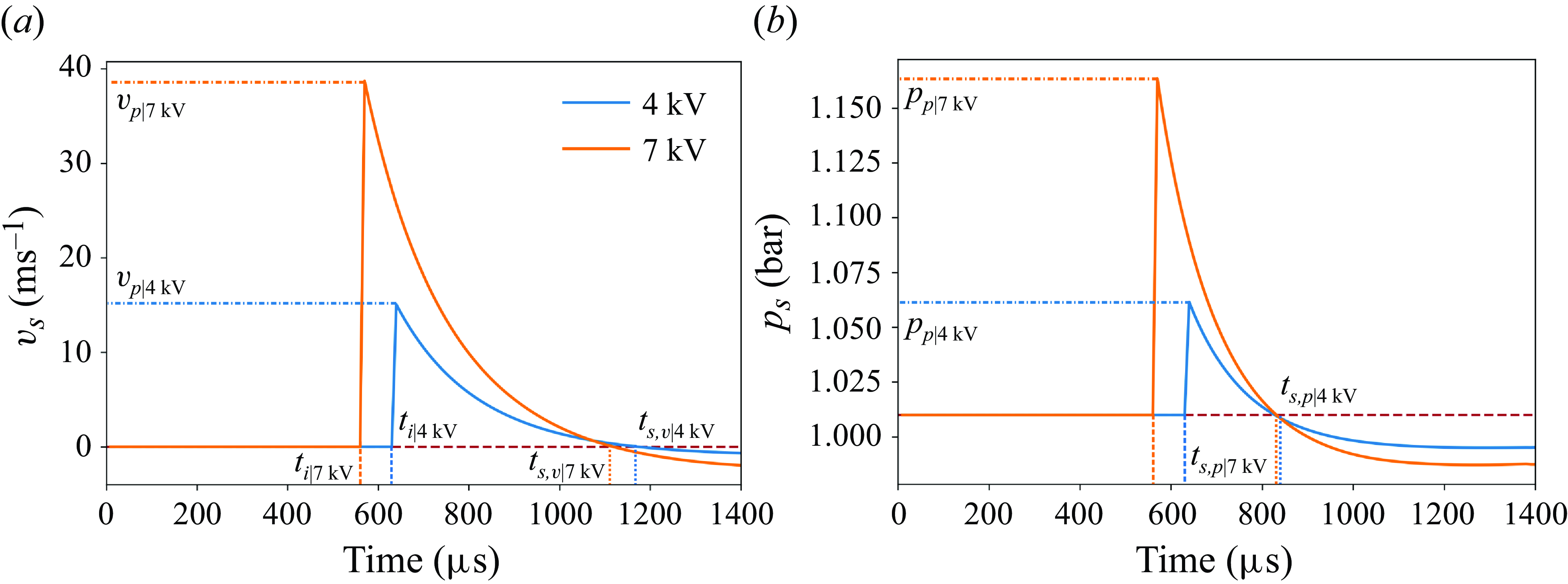
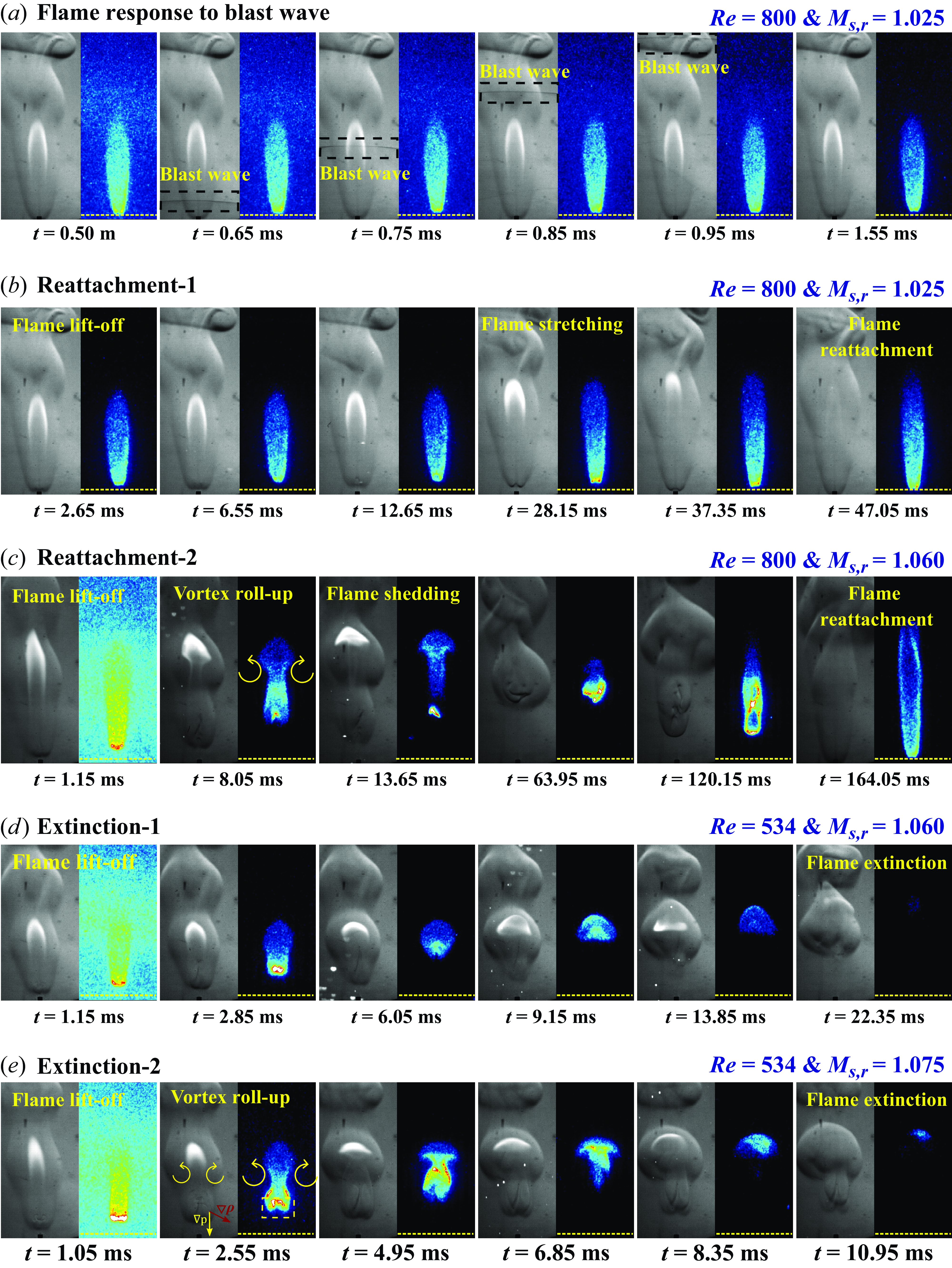


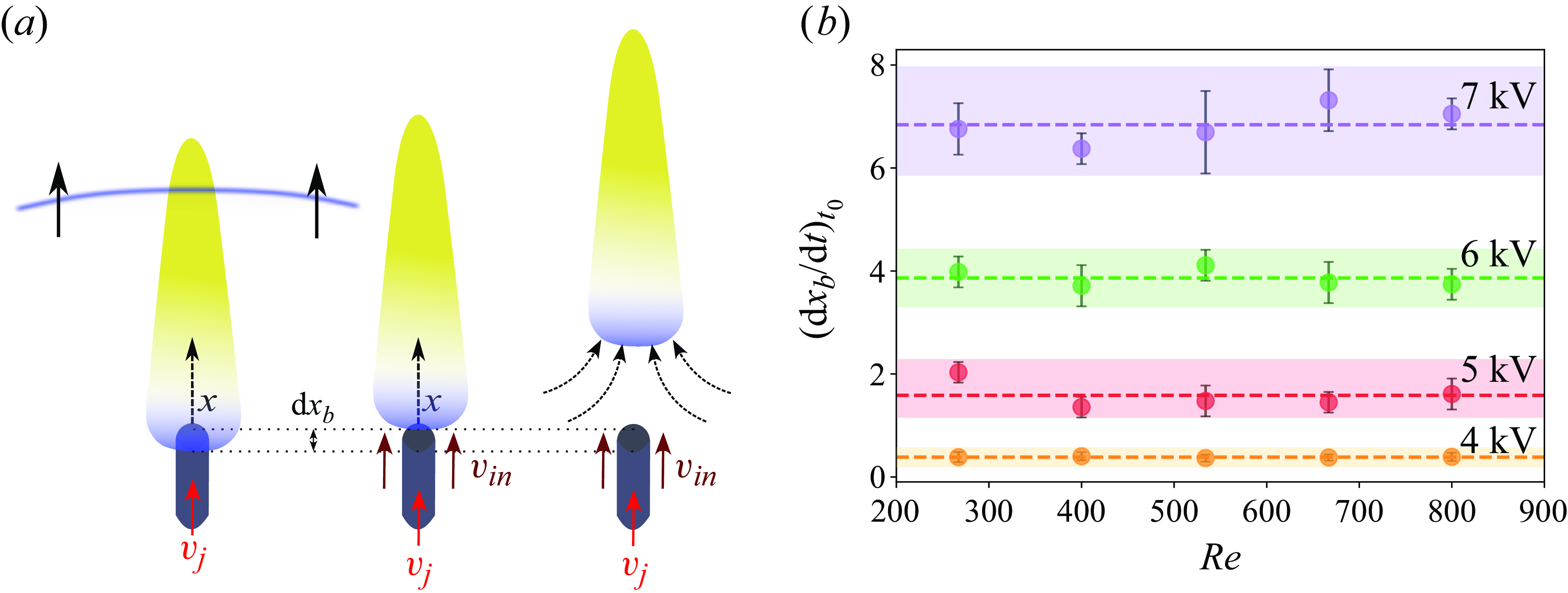

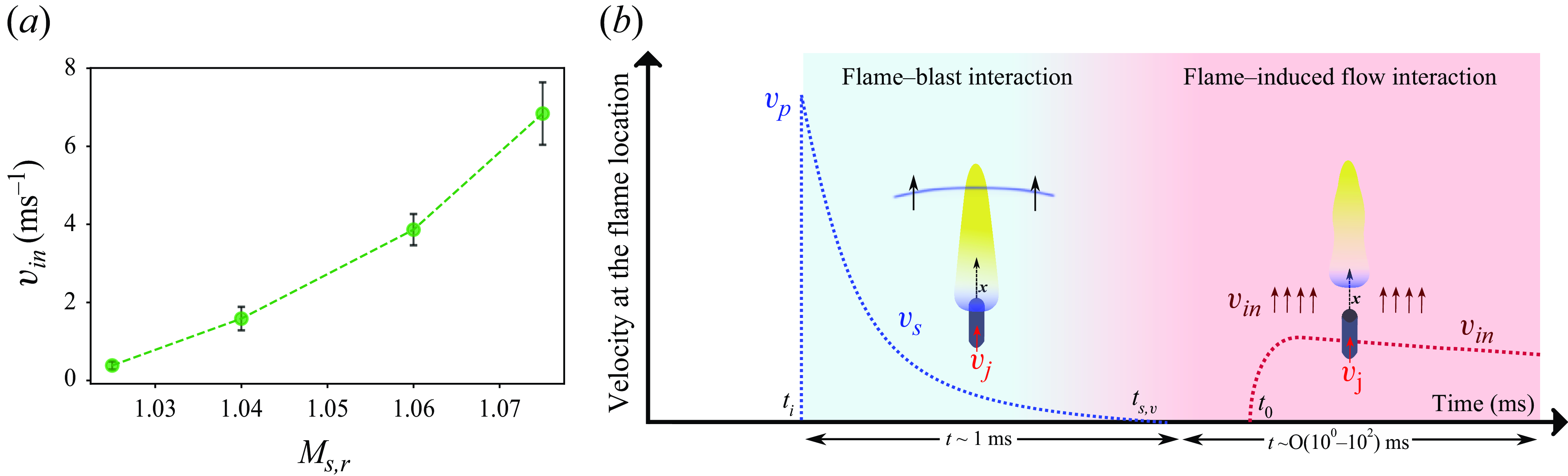


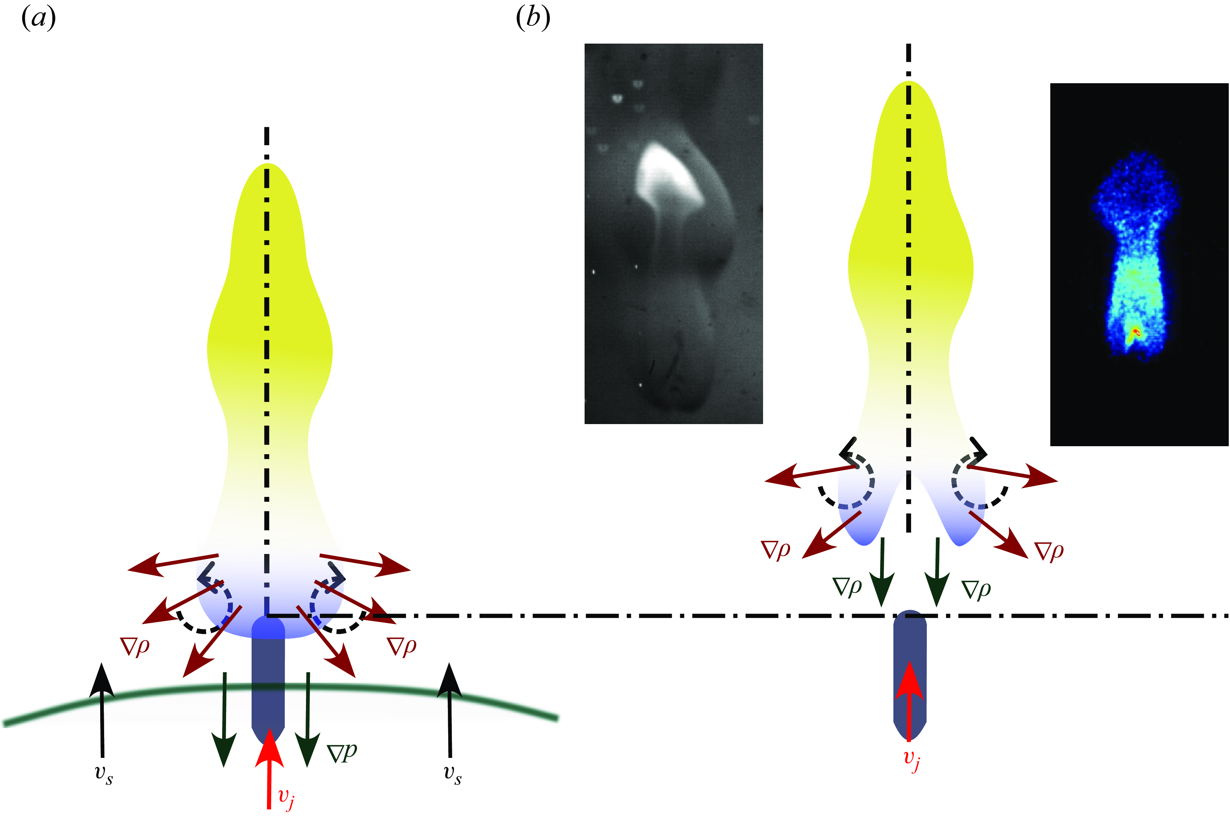
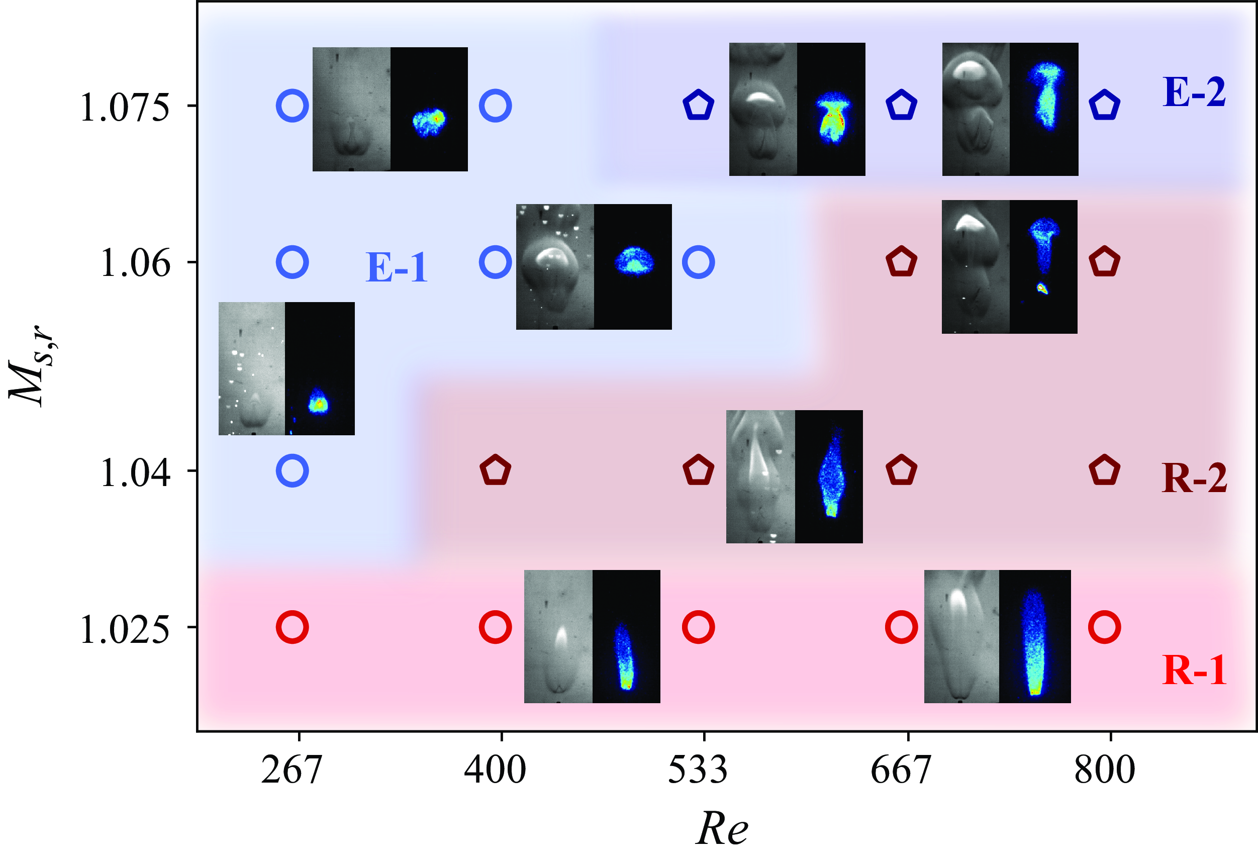
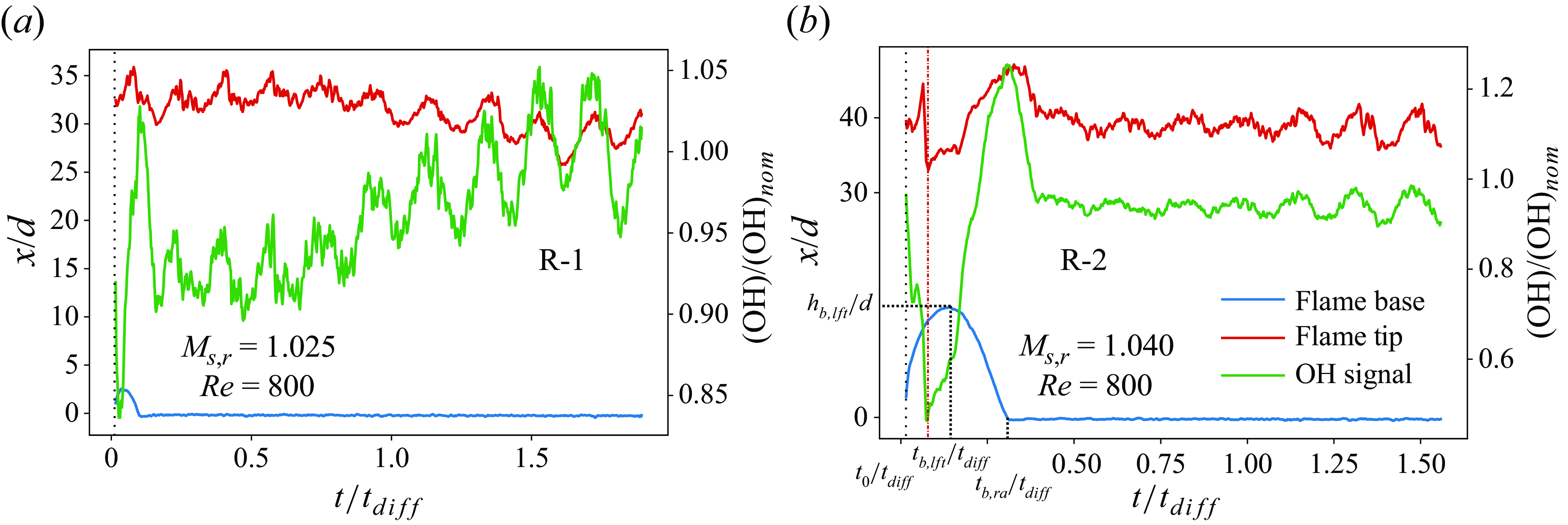


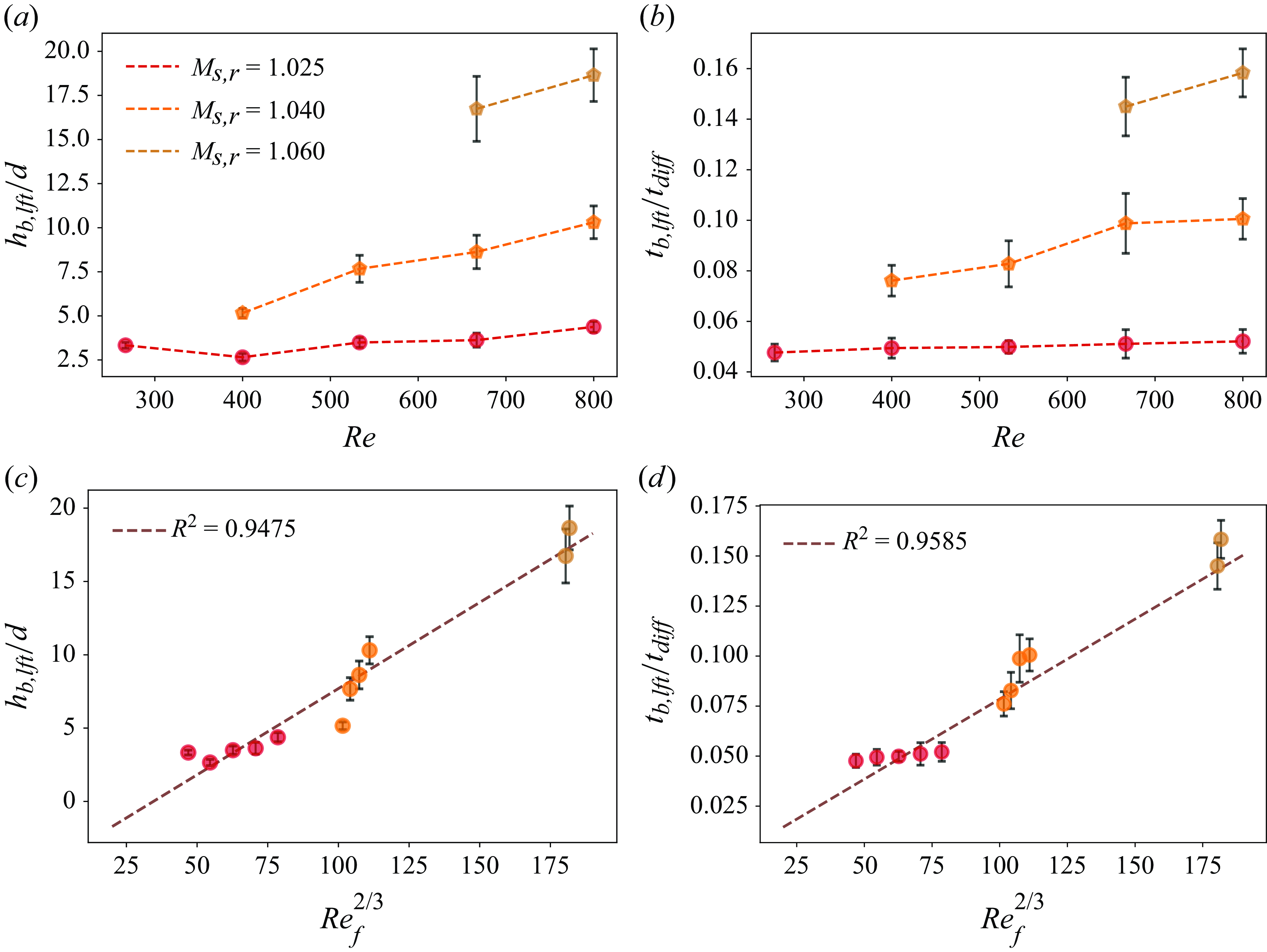


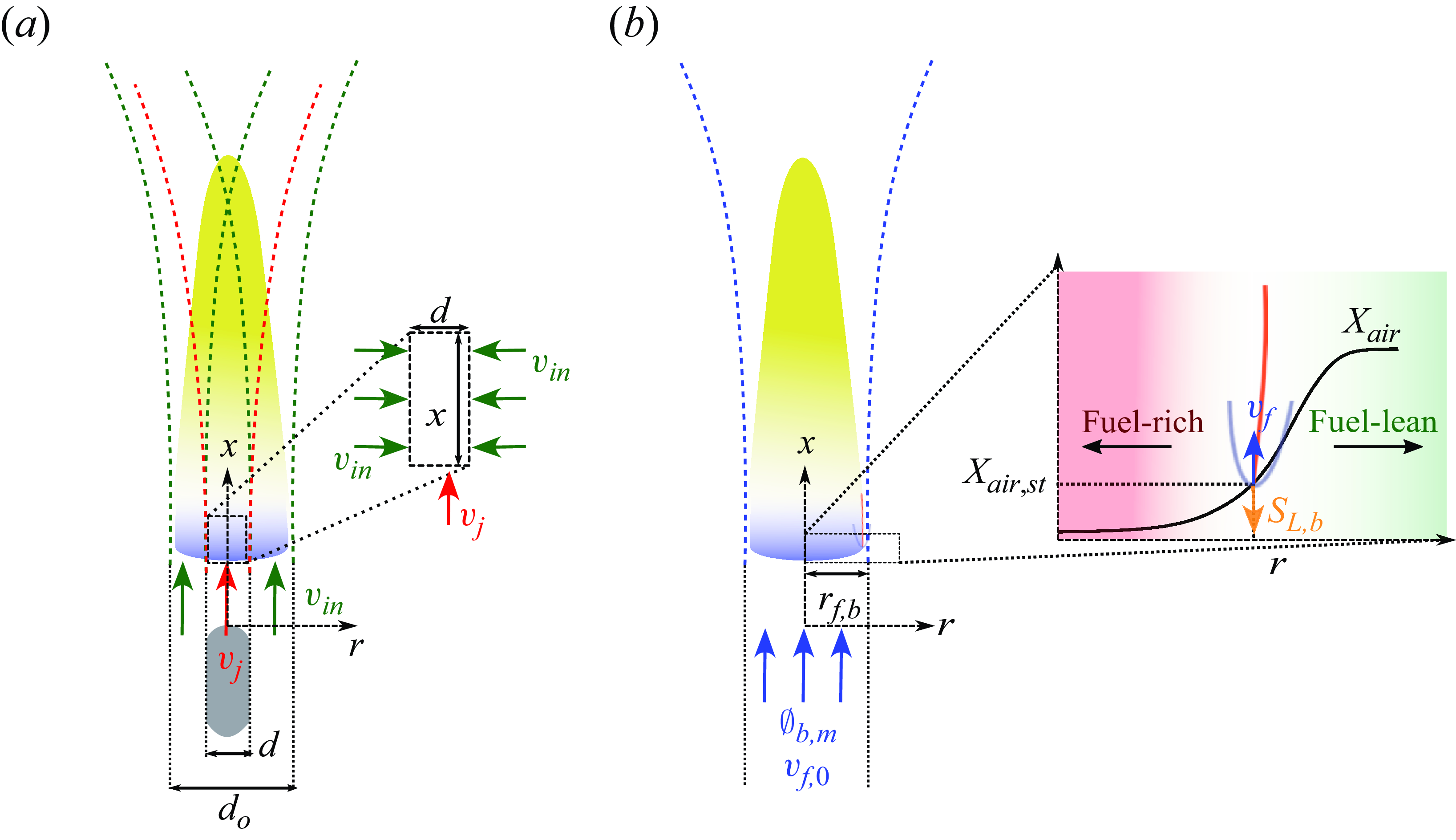
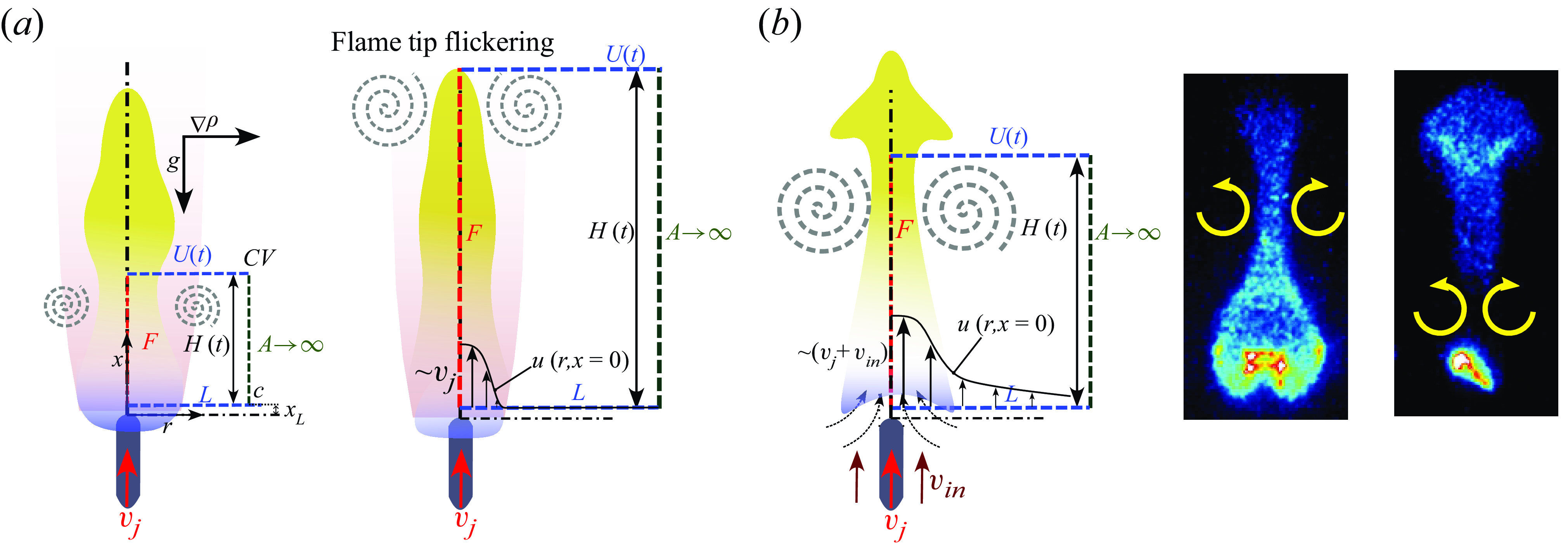


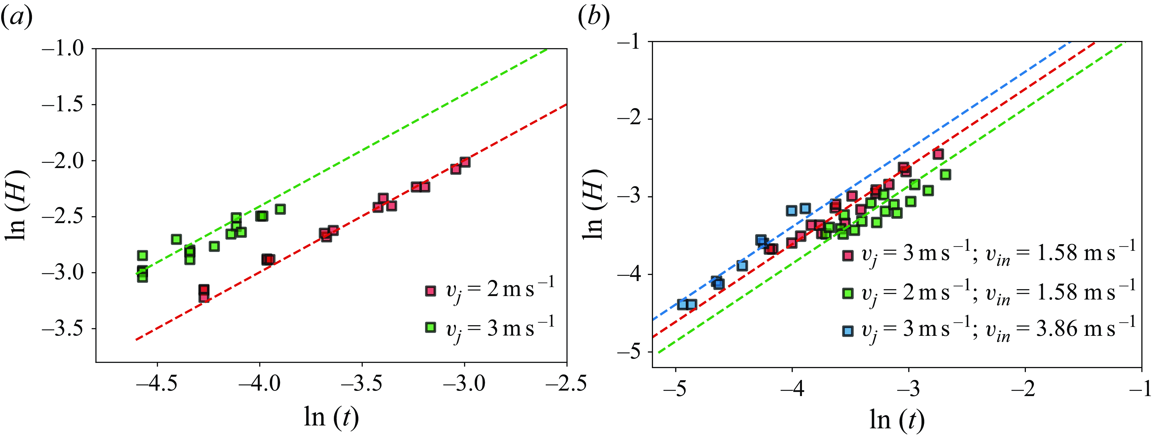


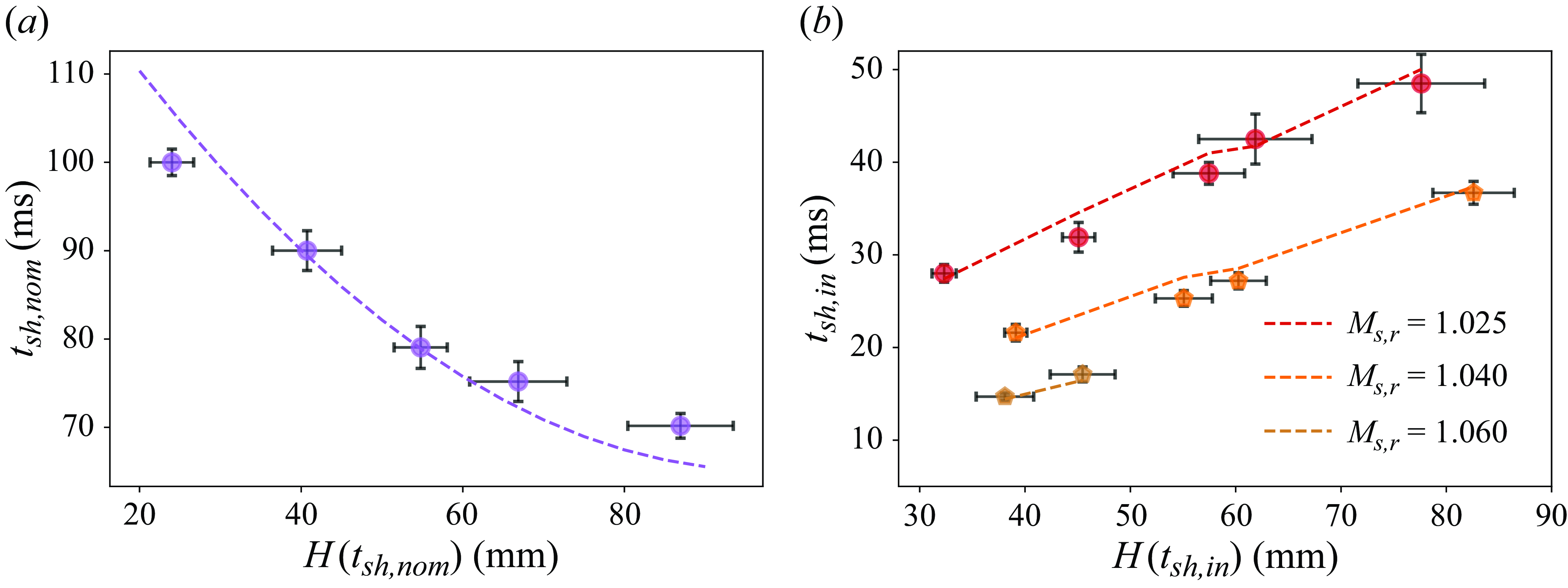


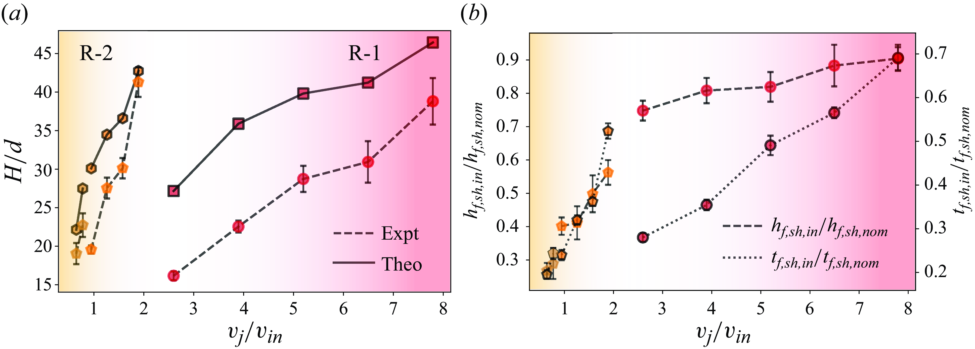

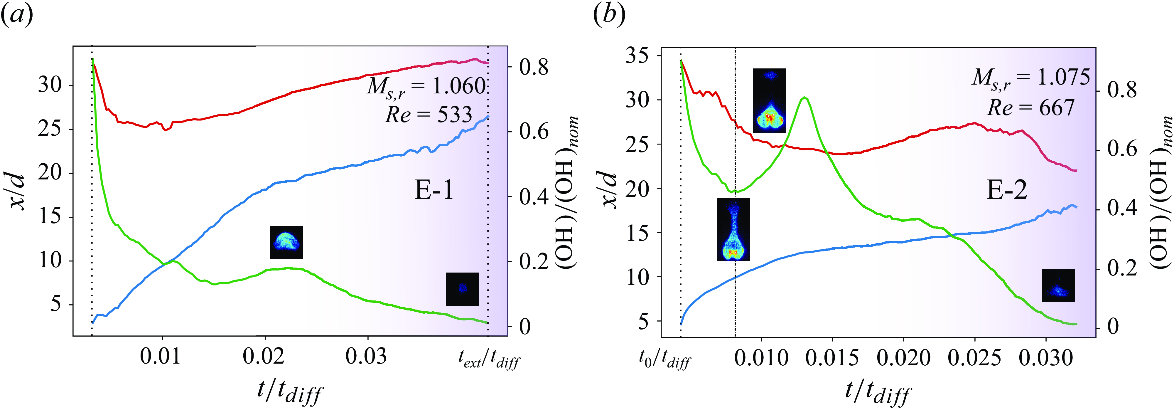
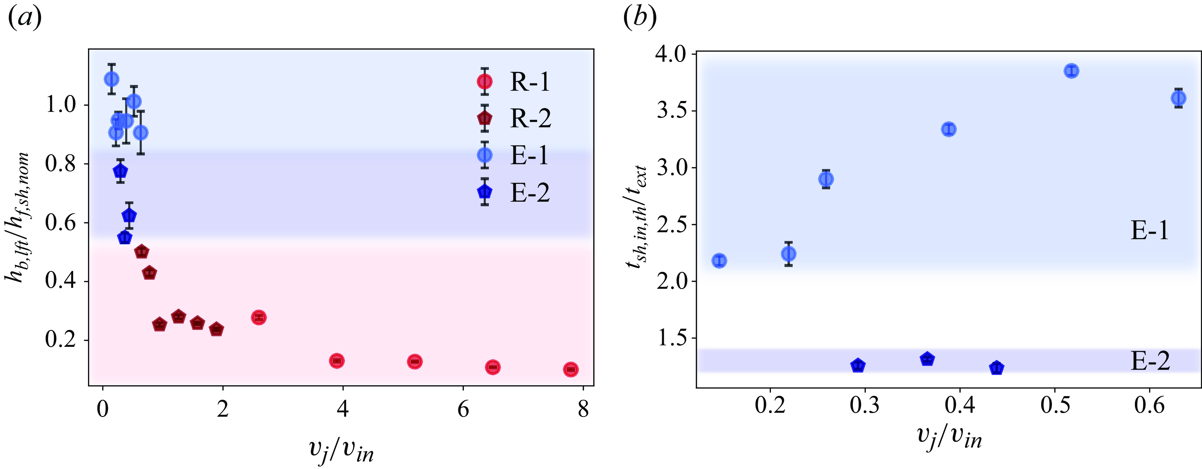


 Open access