


1. Introduction
Darcy's law, which was first proposed by Darcy in 1856 [Reference Darcy19] based on experimental observation of water flowing through beds of sand, describes the relationship between the spontaneous flow discharge rate of steady state through a porous medium, the viscosity of the fluid and the pressure drop over a distance. Later, theoretical/mathematical derivations of Darcy's law were presented in many works, e.g. [Reference Auriault, Borne and Chambon5, Reference Keller25, Reference Lions28, Reference Neuman32, Reference Poreh and Elata36, Reference Sanchez-Palencia38], just to name a few.
In the setting of a periodic pore microstructure, as the period goes to zero, the convergence to the Darcy's law of the Stokes system with no-slip boundary condition posed on the boundary of the pore space was proved by Tartar using the energy method [Reference Tartar40]. Allaire implemented the two-scale convergence method introduced by Nguetseng [Reference Nguetseng33] to derive the Darcy's law and show the convergence [Reference Allaire3, Reference Allaire4]. Prior to the proof of Darcy's law in the 1980s, Brinkman [Reference Brinkman14] studied the viscous force exerted by a flowing flow on a dense swarm of particles by adding a diffusion term to the Darcy's law so as to take into account the transitional flow between boundaries. Brinkman's method was further studied in [Reference Lundgren30, Reference Saffman37, Reference Tam39]. In the case of a porous material where the solid region is much smaller than the fluid part, Levy [Reference Lévy26] and Sanchez-Palencia [Reference Sanchez-Palencia38] proposed the same form of Darcy's law but with a different representation of the permeability tensor $\boldsymbol K$ . Later on, Allaire [Reference Allaire2] showed the continuity of the transition between the two forms of Darcy's laws by considering various ratios between the size of the solid inclusion and the size of the separation. Moreover, instead of considering the porous materials as a periodic structured material, Beliaev [Reference Beliaev and Kozlov9] considered the porous materials as a random and stochastically homogeneous material and deduced the same Darcy's law. Allaire [Reference Allaire1] generalized the homogenization to handle the more realistic micro-geometries of the porous medium where both the solid part and the fluid part are connected. Furthermore, in terms of the fluid–solid interface conditions, a slip boundary condition is considered by Allaire in [Reference Allaire1, Reference Cioranescu, Donato and Ene17]. In the case of the fluid flow through a porous medium subject to a time-harmonic pressure gradient, the permeability depends on the frequency and is referred to as the dynamic permeability. The theory of dynamic permeability is established [Reference Auriault, Borne and Chambon5, Reference Avellaneda and Torquato8, Reference Biot12, Reference Johnson, Koplik and Dashen22] and further developed by Ou [Reference Ou35].
The goal of this paper is to study how the permeability tensor derived from the homogenization approach for porous materials [Reference Tartar40, Reference Tice41] depends on the microstructure of the pore space. Details of this will be presented in § 1.1.
The main tool we use will be the integral representation formula (IRF) for composite materials. Composite materials are materials made from more than one constituent material with different physical or chemical properties. The effective properties of composites, such as elasticity, conductivity and permeability are of great interest in different application fields. Homogenization theory for composite materials has been extensively studied in [Reference Bensoussan, Lions and Papanicolaou10, Reference Milton31, Reference Oleinik, Shamaev and Yosifian34]. Mathematically, for a two-component composite material, the microstructural information is carried into the analytical formulation of the effective properties of the composite. Bergman pioneered the study of analyticity of the effective dielectric constant [Reference Bergman11], and in terms of integral representation of effective material properties, a rigorous basis of integral representation of the effective conductivity is established by Golden and Papanicolaou [Reference Golden and Papanicolaou21], the effective elastic constants by Kantor and Bergman [Reference Kantor and Bergman23], the effective diffusivity in convection-enhanced diffusion was derived by Avellaneda and Majda [Reference Avellaneda and Majda6, Reference Avellaneda and Majda7]. Further enlargements of the domain of analyticity of the IRF of elasticity tensor to the case where one phase is a void or a hard inclusion is studied by Bruno and Leo [Reference Bruno15, Reference Bruno and Leo16].
Unlike the problem set-up for calculating effective material properties such as effective conductivity, elasticity and diffusivity, where the physical property of interest is well defined both in the micro-scale and the macro(homogenized)-scale, the permeability of porous material is by definition an effective property and hence it makes sense only in the macro-scale. To overcome this difficulty, we consider a porous material as the limit case of a two-fluid mixture.
Specifically, we will start with the two-fluid mixture problem studied in [Reference Lipton and Avellaneda29], where the effective property is called the self-permeability. We will derive the IRF for the self-permeability and show that the permeability for a porous material is equal to the limit of the self-permeability when the viscosity of one phase becomes infinite. Similar to the hard/soft inclusion case studied in [Reference Bruno15, Reference Bruno and Leo16], we will extend the domain of analyticity of the IRF to $\infty$ and to $0$
 by an iterative process. As a result, the IRF derived here is valid for porous materials with a solid skeleton as well as for fluid-bubble mixtures. Hence it provides a theoretical connection between the permeability defined in [Reference Tartar40] and the self-permeability for the bubbly fluid studied in [Reference Lipton and Avellaneda29] and any mixture in between these two limiting cases.
The paper is organized as follows. The permeability of a porous material is defined in § 1.1. Section 2 starts with the definition of the self-permeability $\boldsymbol K$ of a two-fluid mixture and the corresponding cell problem, followed by an analysis of the cell problem and the construction of the solution in the vicinity of the two limiting cases of $z=\infty$
 and $z=0$
 . In § 3, the IRF of $\boldsymbol K$
 is obtained by applying the theory of matrix-valued Stieltjes functions. In this section, the spectral representation of $\boldsymbol K$
 is also derived. The relationships between the moments of the measure in the IRF and the geometry of the pore space are derived by comparing these two representations. Section 4 presents the numerical solutions of the cell problem of a special pore structure, which validate the theoretical results given in § 3.
Einstein summation convention is applied unless stated otherwise.
1.1 Definition of permeability from homogenization
Following the convention of homogenization, the space coordinates for the cell problem in the open unit cell $Q=(0,1)^{n}$ for $n=2,3$
 , are denoted by $\mathbf {y}=(y_1, y_2, y_3)$
 . Let $\Omega$
 be a smooth bounded open set and $Q$
 an open unit cube made of two open sets $Q_1$
 , $Q_2$
 and the interface $\Gamma =\text {cl}(Q_1)\cap \text {cl}(Q_2)$
 with cl($A$
 ) being the closure of a set $A$
 . Moreover, $\widetilde {Q_i}$
 denotes the $Q$
 -periodic extension of $Q_i$
 , $i=1,2$
 . Following [Reference Allaire1], we assume that (1) $Q_1$
 and $Q_2$
 have strictly positive measures in cl($Q$
 ). (2) The set $\widetilde {Q_i}$
 is open with $C^{1}$
 boundary and is locally located on one side of its boundary, $i=1,2$
 , and $\widetilde {Q_1}$
 is connected. (3) $Q_1$
 is connected with a Lipschitz boundary. In addition, we consider the case of inclusion, i.e. $Q_2\cap \partial Q=\emptyset$
 .
.
Consider $\epsilon >0$ much smaller than the size of $\Omega$
 and $\epsilon Q$
 -periodically extend $\epsilon Q_1$
 in the entire space. $\Omega _\epsilon$
 denotes the intersection of $\Omega$
 and this $\epsilon Q$
 -periodically extended structure. In [Reference Tartar40], the permeability is derived from the Stokes equation in $\Omega _\epsilon$
 , which reads: find $\mathbf {u}^{\epsilon }\in H_0^{1}(\Omega _\epsilon )^{n}$
 and $p^{\epsilon } \in L^{2}(\Omega _\epsilon )/\mathbb {R}$
 such that

where $\mathbf {f}\in L^{2}(\Omega )$ is independent of $\epsilon$
 and the viscosity $\mu$
 is a constant ($\mu$
 is set to 1 in [Reference Tartar40, Reference Tice41]). See figure 1 for an example of the unit cube. Note that the superscript $\epsilon$
 is used to signify that the solutions $\mathbf {u}^{\epsilon }$
 and $p^{\epsilon }$
 depend on $\epsilon$
 . To be able to prove the convergence of $(\mathbf {u}^{\epsilon },p^{\epsilon })$
 as $\epsilon \rightarrow 0$
 , it is necessary to extend these solutions from $\Omega _\epsilon$
 to $\Omega$
 so they are defined in the same spatial domain. In [Reference Tartar40, Reference Tice41], $\mathbf {u}^{\epsilon }$
 was extended by zero and $p^{\epsilon }$
 by a properly defined extension operator with their extensions denoted by $\hat {\mathbf {u}^{\epsilon }}$
 and $\hat {p^{\epsilon }}$
 , respectively. As $\epsilon \rightarrow 0$
 ,
,

and the limit functions satisfy the following Darcy's law [Reference Tartar40]

where the permeability tensor $\boldsymbol K^{(D)}$ is defined as

with $\mathbf{e} _i$ denoting the unit vector in the $i$
 -th direction and $\mathbf{u} _D^{j}$
 the unique solution of the following boundary value problem

in the space $\mathring {H}(Q_1): = \{ \mathbf {v}: \mathbf {v}\in H^{1}(Q_1)^{n}\vert \; \text {div}_{\mathbf {y}} \mathbf {v} = 0, \mathbf {v}\vert _{\Gamma } = {{\mathbf 0}}, Q \text {-periodic} \}$ . Note that the superscript $j$
 of $\mathbf {u}$
 and $p$
 signifies the solutions corresponding to the force term $\mathbf{e} _j$
 .
.

FIG. 1. Sample illustration of a periodic cell.
Since $\mu$ is set to 1 in [Reference Tartar40, Reference Tice41], the permeability $\boldsymbol K$
 presented there is related to $\boldsymbol K^{(D)}$
 by $\boldsymbol K^{(D)}={\boldsymbol K}/{\mu }$
 . For future analysis, we will derive here the quadratic form representation of the permeability. We start by observing that for incompressible fluid, we have

Therefore, (1.3) can be expressed as

after applying the divergence theorem, the periodicity of $\mathbf {u}$ , $p$
, $p$ and the no-slip conditions on $\Gamma$
 . Here we have used the Frobenius inner product of matrices $\mathbf {A} : \mathbf {B} = \sum _{i,j = 1} A_{ij}B_{ij}$
 . In terms of the usual notion of the symmetric part and the antisymmetric part of vector field $\nabla \mathbf{u}$

the right-hand side of equation (1.5) becomes $\int _{Q_1} 2\mu (e(\mathbf{u} _D^{j})+\tilde {e}(\mathbf{u} _D^{j})) : e( \mathbf{u} _D^{i} )\,{\rm d}\mathbf {y} =\int _{Q_1} 2\mu e(\mathbf{u} _D^{j}) : e(\mathbf{u} _D^{i})\,{\rm d}\mathbf {y}$ because the Frobenius product of a symmetric matrix and an antisymmetric matrix must be 0. Therefore we have the quadratic form of permeability tensor $\boldsymbol K^{(D)}$

2. Approximation of flow in porous medium by a two-phase Stokes flow
In this section, we consider the system for porous materials (1.4) as one of the limiting cases of the two-fluid problem described below, which is the same as the one studied in [Reference Lipton and Avellaneda29] with the exception that the fluid viscosity here can be complex-valued. It is easy to check that the homogenization process in [Reference Lipton and Avellaneda29] stays valid after making small modifications to accommodate the complex valued viscosity described below.
Let $\Omega$ , $Q$
, $Q$ and $\epsilon$
 be the same as in § 1.1. $Q_2$
 is still the inclusion in the periodic cell. Consider the ${\epsilon Q}$
 -periodic extension of $\epsilon Q_1$
 (${\epsilon }Q_2$
 ) and denote by $\Omega _{1{\epsilon }}$
 ($\Omega _{2\epsilon }$
 ) its intersection with $\Omega$
 . We note that $\Omega _{1{\epsilon }}$
 (region of the hosting fluid) is the same as $\Omega _\epsilon$
 in the previous section. Suppose $\Omega _{1{\epsilon }}$
 is occupied by fluid with viscosity $\mu _1>0$
 and $\Omega _2$
 by fluid with viscosity $z\mu _1$
 with $z\in \mathbb {C}$
 . The interface $\tilde {\Gamma } = \partial \Omega _{1{\epsilon }} \cap \partial \Omega _{2{\epsilon }}$
 is such that $\Omega _{1{\epsilon }}\cup {\tilde {\Gamma }\ \cup \ }{\Omega _{2{\epsilon }}} = \Omega$
 . For the ease of notation, we define the stress tensor $\boldsymbol {\tau }(\mathbf {u},\boldsymbol \mu )$
 of a fluid with viscosity $\mu$
 , velocity field $\mathbf {u}$
 and pressure field $p$
 as
as

Let $\chi _i$ be the characteristic function of $\Omega _{\epsilon i}$
 , $i=1,2$
 . Consider the viscosity function

The two-fluid problem is given by the following Stokes system

where $\boldsymbol \pi =\boldsymbol \tau (\mathbf {u}^{\epsilon },p^{\epsilon }, \boldsymbol {\xi }^{\epsilon })$ , $\mathbf {f}$
 is a square integrable momentum source independent of $\epsilon$
 , $[\kern-1pt[ \cdot ]\kern-1pt]$
 the jump across the interface $\tilde {\Gamma }$
 and $\mathbf {n}$
 is the outward unit normal of $\partial \Omega _{2\epsilon }$
 . The second jump condition in (2.3) means the traction can only jump in the normal direction. Also note that the superscript $\epsilon$
 is used to signify that the solutions $\mathbf {u}^{\epsilon }$
 and $p^{\epsilon }$
 depend on $\epsilon$
 .
.
It is shown in [Reference Lipton and Avellaneda29] that as $\epsilon \to 0$ , $\mathbf {u}^{\epsilon }$
 and the properly normalized $p^{\epsilon }$
 , which is denoted by $\hat {p}^{\epsilon }$
 , converge as follows

where $\mathbf {u}^{0}$ and $P$
 satisfy the homogenized system:

where the components of $\boldsymbol K$ , which is referred to as the self-permeability in [Reference Lipton and Avellaneda29], is defined as

with $\mathbf {u}^{{i}}$ being the unique solution to the cell problem posed in the function space $H(Q)$
 , which is defined in (2.7),

where $\boldsymbol \mu (\mathbf {y};z)=\mu _1 \chi _1(\mathbf {y})+z\mu _1 \chi _2(\mathbf {y})$ with $\chi _m$
 being the characteristic functions of $Q_m$
 , $m=1,2,$
 and $\boldsymbol \pi =\boldsymbol \tau (\mathbf {u}^{k},p^{k},\boldsymbol \mu )$
 , cf. (2.1). Note that the superscript $i$
 is used to signify that $\mathbf {u}^{i}$
 and $p^{i}$
 are solutions to the cell problem (2.6) with the force term $-\mathbf{e} _i$
 , $i=1,\ldots,n$
 .
.
2.1 Function spaces
Let $\mathcal {R}(Q_2)$ denote the space of rigid body displacements in $Q_2$
 , i.e. $\mathbf {u} = \mathbf {A}\mathbf {y} + \mathbf {b}$
 with constant skew-symmetric matrix $A$
 and constant vector $\mathbf {b}$
 in $Q_2$
 . We start with the space of admissible functions for the velocity

where $\mathbf {n}$ is the outward unit normal of $\partial Q_2$
 . $H (Q)$
 is endowed with the inner product

The induced norm is denoted by $\left \lVert {\mathbf {u}}\right \rVert _{Q}^{2} := (\mathbf {u},\mathbf {u})_Q$ . Note that we have $H(Q)\cap \mathcal {R}(Q)=\{\mathbf {0}\}$
 because $\mathbf {A} = 0$
 due to the $Q$
 -periodicity and $\mathbf {u} \cdot \mathbf {n} = 0$
 implies $\mathbf {b} = {{\mathbf 0}}$
 . We observe that if $\mathbf {u} \in H(Q)$
 then $\mathbf {u} \in H^{1}(Q)^{n}$
 by the following argument. Obviously, $\mathbf {u} \in L^{2}(Q)^{n}$
 . To prove ${\partial u_i}/{\partial y_j} \in L^{2}(Q)$
 for $i,j = 1,2,3$
 , let $\phi$
 be any $C^{\infty }$
 test function compactly supported in $Q$
 and $h$
 be the $i$
 -th component $u_i$
 for any $i$
 . Then

here we used $[\kern-1pt[ h ]\kern-1pt] = {{\mathbf 0}}$ . Now we can define a candidate function $\mathbf {g}$
 such that

then clearly $\mathbf {g}\in L^{2}(Q)^{n}$ and $\left < h,\nabla \phi \right > = -\left < g,\phi \right >$
 , where $\left <\cdot \right >$
 denotes the usual $L^{2}$
 inner product. Therefore ${h} \in H^{1}(Q)$
 and hence $u_i \in H^{1}(Q), \ i=1,\ldots,n$
 .
.
Next, we show that $\| \cdot \|_Q$ is equivalent to the usual $H^{1}$
 norm, i.e., there exist constants $B_1$
 and $B_2$
 such that

Because $H^{1}(Q)\cap \mathcal {R}(Q)=\{0\}$ , by theorem 2.5 in [Reference Oleinik, Shamaev and Yosifian34], there exists a Korn's constant $C_1$
 such that

where $C_1$ depends only on $Q$
 . Therefore, we can take $B_1=\sqrt {2\mu _1}C_1$
 . To emphasize the dependence on $Q$
 , we will write it as $B_1(Q)$
 . On the other hand, according to the orthogonal decomposition that $\nabla \mathbf {u} = e(\mathbf {u}) + \tilde {e}(\mathbf {u})$
 , see (1.6),

therefore $B_2 = \sqrt {2\mu _1}$ . The reason for introducing the $H(Q)$
 -norm is that the self-permeability in (2.5) can be represented in terms of the inner product. More specifically, using (2.5), (2.6) and the fact that $\overline {\mathbf{e} _i}=\mathbf{e} _i$
 , by a calculation similar to (1.5) and taking into account the interface condition $\mathbf {u}\cdot \mathbf {n}=0$
 and the jump conditions in (2.6), (2.5) can be expressed in the following form

and its conjugate transpose $\boldsymbol K^{*}:=\overline {\boldsymbol K^{T}}$ is
is

2.2 Weak solution of the cell problem (2.6)
The weak formulation of the cell problem (2.6) is

From this, we see that the solutions satisfy the following symmetry

Define the sesquilinear form on $H(Q)$

It is clear that $a(\mathbf {u},\mathbf {v})$ is bounded in $H(Q)$
 . To check the coercivity, assume $\mathbf {u}^{k} \neq 0$
 and define the parameter

then $0\leq \lambda \leq 1$ . We note that

and hence as long as 0 is not on the line segment joining $z$ and 1, there exist $\alpha (z):=\min _{0\le \lambda \le 1} |\lambda z+1-\lambda |>0$
 such that

Therefore for $z\in \mathbb {C}\backslash \left \lbrace \Re {z}\leq 0\right \rbrace$ , by the Lax–Milgram lemma [Reference Brenner and Scott13, chapter 2], there exists a unique weak solution $\mathbf {u}^{k}\in H(Q)$
 to the cell problem (2.6) and with the solution $\mathbf {u}^{k}$
 , we can construct $p^{k} \in L^{2}(Q)/\mathbb {C}$
 .
.
Since $\alpha (z)$ is a continuous function in $z$
 , the coercivity of the sesquilinear form can be applied to conclude that $\mathbf {u}^{k}$
 is analytic in $z$
 and its $m$
 -th derivative, $m\ge 1$
 , satisfies the following recursive equation

As a result, $\boldsymbol K(z)$ is also analytic for $z\in \mathbb {C}\backslash \left \{ \Re {z}\leq 0\right \}$
 . To relate the two-fluid problem with $\boldsymbol K^{(D)}$
 , we adapt the method used in [Reference Bruno and Leo16] to study the behaviour of $\boldsymbol K(z)$
 near $z=\infty$
 in the following section.
2.3 Analyticity of the solution for large $|z|$

Let $w:=\frac {1}{z}$ and consider $Q$
 -periodic solution in the series form near $w=0$

where the $\mathbf {e}$ is an arbitrary constant unit vector. To set up the notation, we denote the restrictions of $\mathbf{u} _k$
 , $p_k$
 in $Q_2$
 (inclusion) and $Q_1$
 as $\mathbf {u}^{in}_k$
 , $p^{in}_k$
 and $\mathbf {u}^{out}_k$
 , $p^{out}_k$
 respectively and define

By substituting (2.20) into (2.6) with the viscosity defined in (2.2), taking into account the additional two interface conditions $\mathbf {u}\cdot \mathbf{n} =0$ and $[\kern-1pt[ \mathbf {u} ]\kern-1pt] =0$
 , followed by equating terms of the same order with respect to $w$
 , we arrive in the following equations in $Q_1$
 :
:


and in $Q_2$ :
:


and the following interface conditions on $\Gamma$


We introduce the following spaces, $i=1,2$

Note that $H(Q_1)\cap \mathcal {R}(Q_1)=\{{{\mathbf 0}}\}$ because $\partial Q \subset \partial Q_1$
 . For $H(Q_2)$
 , the boundary condition $\mathbf {u}\cdot \mathbf{n} =0$
 implies $H(Q_2)\cap \mathcal {R}(Q_2)=\{{{\mathbf 0}}\}$
 because of the extra condition $(\mathbf {v},\mathcal {R}(Q_2))_{H^{1}(Q_2)}=0$
 [Reference Oleinik, Shamaev and Yosifian34]. Therefore, $H(Q_i)$
 and $\mathring {H}(Q_i)$
 are equipped with inner product $(\mathbf {u},\mathbf {v})_{Q_i} = \int _{Q_i} 2\mu _1e(\mathbf {u}) : \overline {e(\mathbf {v})}\,{\rm d}\mathbf {y}$
 and Korn's inequalities are valid in $H(Q_i)$
 , $i=1,2$
 .
.
Lemma 2.1 Let $Q_2$ be a connected, open bounded set such that $\partial Q_2 \cap \partial Q=\emptyset$
 and $\partial Q_2$
 is in $\mathcal {C}^{k,\sigma }$
 , $k,\sigma \ge 0$
 , $k+\sigma \ge 2$
 . For any vector field $\mathbf {u}^{in} \in H(Q_2)$
 , there exists a unique weak solution $\mathbf {u}^{out}(\mathbf {y};\mathbf {f}^{out})\in H(Q_1)$
 that satisfies the following system

where in our context, $\mathbf {f}^{out} = {{\mathbf 0}} \text { or } \mathbf {f}^{out} = -\mathbf {e}$ , a constant unit vector. Moreover,

where the positive constants $B_1(Q_{{1}})$ is defined in (2.10) and $E_1\ge 1$
 depends only on $Q_1$
 and $Q_2$
 .
.
Proof. To handle the inhomogeneous boundary condition, we proceed as follows. By [Reference Kato, Mitrea, Ponce and Taylor24, corollary 3.2], there exists a bounded, divergence free extension $T(\mathbf {u}^{in})$ of $\mathbf {u}^{in}$
 to a small neighbourhood $O$
 of $Q_2$
 and vanishes at $\partial O\subset Q_1$
 such that

where $E_1\ge 1$ depends only on $Q_1$
 and $Q_2$
 . Furthermore, the extension $T(\mathbf {u}^{in})$
 on $O$
 can be extended periodically to $\mathbb {R}^{n}$
 [Reference Conca18] since $T(\mathbf {u}^{in})$
 vanishes on $\partial O$
 and hence on $\partial Q$
 . We denote the restriction $T(\mathbf {u}^{in})|_{Q_1}$
 as $\tilde {\mathbf {u}}^{out}\in H(Q_1)$
 and $\mathring {\mathbf {u}}^{out} := \mathbf {u}^{out} - \tilde {\mathbf {u}}^{out} \in \mathring {H}(Q_1)$
 and (2.30) becomes

Consider the variational formulation: find $\mathring {\mathbf {u}}^{out} \in \mathring {H}(Q_1)$ such that $\forall \Phi \in \mathring {H}(Q_1)$
 ,
,

The right-hand side of (2.34) can be bounded as follows

The sesquilinear form $\int _{Q_1} 2\mu _1 e( \mathring {\mathbf {u}}^{out}) : \overline {e(\Phi )}\,{\rm d}\mathbf {y}$ is clearly bounded and coercive with constant 1. Hence by the Lax–Milgram lemma there exists a unique weak solution $\mathring {\mathbf {u}}^{out}\in \mathring {H}(Q_1)$
 to (2.33) such that $\left \lVert {\mathring {\mathbf {u}}^{out}}\right \rVert _{Q_1}\le (({1}/{B_1(Q_{{1}})})\left \lVert {\mathbf {f}^{out}}\right \rVert _{L^{2}(Q_1)} + \left \lVert {\tilde {\mathbf {u}}^{out}}\right \rVert _{Q_1})$
 . In terms of $\mathring {\mathbf {u}}^{out}$
 , $\mathbf {u}^{out}$
 can be expressed as $\mathbf {u}^{out} = \tilde {\mathbf {u}}^{out} + \mathring {\mathbf {u}}^{out}$
 and satisfies the estimate

To show the solution $\mathbf {u}^{out}$ is unique, suppose $\mathbf {u}^{out}_1$
 and $\mathbf {u}^{out}_2$
 both solve (2.30) then the difference ${{\mathbf {w}}}^{\text {diff}} = \mathbf {u}^{out}_1 - \mathbf {u}^{out}_2 \in \mathring {H}(Q_1)$
 must satisfy

Hence ${{\mathbf {w}}}^{\text {diff}}=0$ in $Q_1$
 because ${{\mathbf {w}}}\in \mathring {H}(Q_1)$
 . We note the two special cases:


where $|Q_1|$ is the volume of $Q_1$
 .
.
Lemma 2.2 Let $Q_2$ satisfy the same assumptions as those in lemma 2.1. For any pair of $(\mathbf {u}^{out}, p^{out}) \in H(Q_1) \times L^{2}(Q_1)/ \mathbb {C}$
 that satisfies (2.30), there exists a unique vector $\mathbf {u}^{in}(\mathbf {y};\mathbf {f}^{in})\in H(Q_2)$
 that satisfies the Stokes equation with continuity of tangential traction on $\Gamma$

where in our context, $\mathbf {f}^{in} = {{\mathbf 0}} \text { or } \mathbf {f}^{in} = -\mathbf {e}$ . Moreover,

and $E_1(Q_1)$ , $B_1(Q_1)$
 and $B_1(Q_2)$
 depend only on $Q$
 and $\Gamma$
 .
.
Proof. Take ${\Phi } \in H(Q_2)$ , the variation formulation for the PDE is

For the ease of notation, let $\boldsymbol \pi ^{in}:=\boldsymbol \tau (\mathbf {u}^{in},\mu _1,p^{in})$ and $\boldsymbol \pi ^{out}:=\boldsymbol \tau (\mathbf {u}^{out},\mu _1,p^{out})$
 where the stress function $\boldsymbol \tau$
 is defined in (2.1). Applying integration by parts on the left-hand side, followed by an application of the divergence theorem leads to

Let $\mathbf {t}$ denote the unit vector in the tangent plane such that $\mathbf {t}\cdot \mathbf{n} = 0$
 . The conditions on $\Gamma$
 in (2.38) imply

With these observations and the fact that $\boldsymbol \pi ^{in}$ is symmetric, the first term in (2.39) can be expressed as

and hence the variational form (2.39) becomes for all $\Phi \in H(Q_2)$

To bound the right-hand side of (2.40), we first extend $\Phi \in H(Q_2)$ by the operator $T$
 described in (2.32)

$T(\Phi )$ rapidly decays to zero in a small neighbourhood of $Q_2$
 and stays $0$
 for the rest of $Q_1$
 . The restriction of $T(\Phi )$
 in $Q_1$
 , denoted by $\Phi ^{out}$
 , has the following estimate

Hence

Therefore the right-hand side of (2.40) is bounded by

Finally, by the Lax–Milgram lemma a unique solution $\mathbf {u}^{in}$ exists such that

The construction of the solution for $z$ with large magnitude will be carried out using the following steps.
(i) $O(w^{-1})$
: Consider the system of (2.24) and (2.27) for $\mathbf{u}_0^{in}(\mathbf {y};\mathbf {e})\in H(Q_2)$.
(2.44)\begin{equation} \left \{\begin{array}{@{}ll} {\rm div}_{\mathbf{y}} \left( 2\mu_1 e(\mathbf{u}_0^{in}) \right) = {{\mathbf 0}} & \text{in } Q_2\\ 2\mu_1e(\mathbf{u}_0^{in}) \cdot \mathbf{n} = C(\mathbf{y}) \mathbf{n} & \text{on } \Gamma \end{array} \right. \end{equation}The variational formulation is(2.45)\begin{equation} -\int_{\Gamma} \bar{\mathbf{v}}\cdot 2\mu_1e(\mathbf{u}_0^{in}) \cdot\mathbf{n} - \int_{Q_2}2\mu_1 e(\mathbf{u}_0^{in}) : \overline{e(\mathbf{v})} = 0 \quad \forall \mathbf{v}\in H(Q_2) \end{equation}The first term vanishes because of the boundary conditions. Hence\[ \mathbf{u}_0^{in}(\mathbf{y};\mathbf{e}) = {{\mathbf 0}} \text{ in } Q_2 \text{ because}\ H(Q_2)\perp \mathcal{R}(Q_2). \](ii) $O(w^{0})$
in $Q_1$: Solve the system of (2.29) and (2.22) for $\mathbf{u}_0^{out}(\mathbf {y};\mathbf {e}) \in H(Q_1)$.
(2.46)\begin{equation} \left \{\begin{array}{@{}ll} {\rm div}_{\mathbf{y}} \left( 2\mu_1 e(\mathbf{u}_0^{out}) - p_0^{out}\mathbf{I} \right)={-}\mathbf{e} & \text{in } Q_1\\ \mathbf{u}_0^{out} = \mathbf{u}_0^{in} = {{\mathbf 0}} & \text{on } \Gamma \end{array}\right. \end{equation}An application of lemma 2.1 and (2.37) leads to the following result(2.47)\begin{equation} \left\lVert{\mathbf{u}_0^{out}}\right\rVert_{Q_1} \leq \frac{\sqrt{|Q_1|}}{B_1(Q_{{1}})} + 2E_1 \left\lVert{\mathbf{u}^{in}_0}\right\rVert_{Q_2}= \frac{\sqrt{|Q_1|}}{B_1(Q_{{1}})} \end{equation}(iii) $O(w^{0})$
in $Q_2$: Consider the system of (2.25) and (2.28) for $\mathbf{u}_1^{in}\in H(Q_2)$:
\[ \left\{\begin{array}{@{}ll} {\rm div}_{\mathbf{y}}\left( 2\mu_1 e(\mathbf{u}_1^{in}) - p_0^{in}\mathbf{I} \right) ={-}\mathbf{e} & \text{in } Q_2\\ \mathbf{n}\times\mathbf{n}\times\left[\left( \left( 2\mu_1 e(\mathbf{u}_0^{out}) - p_0^{out}\mathbf{I} \right) - \left( 2\mu_1 e(\mathbf{u}_{1}^{in}) - p_0^{in}\mathbf{I} \right) \right)\cdot \mathbf{n}\right] = {{\mathbf 0}} & \text{on } \Gamma \end{array}\right. \]By applying lemma 2.2 and (2.43) with $\mathbf {f}^{out} = -\mathbf {e}$ and $\mathbf {f}^{in} = -\mathbf {e}$, we obtain
(2.48)\begin{equation} \left\lVert{\mathbf{u}_{1}^{in}}\right\rVert_{Q_2} \leq {C_1E_1},\quad {C_1}:=\frac{\sqrt{|Q_2|}}{B_1(Q_{{2}})} + 2\frac{\sqrt{|Q_1|}}{B_1(Q_{{1}})} \end{equation}(iv) Induction step, $k\geq 1$
: Given $\mathbf{u}_{k}^{in} \in H(Q_2)$ and $\mathbf{u}_{k-1}^{out}\in H(Q_1)$, find $\mathbf{u}_{k+1}^{in}(\mathbf {y};{{\mathbf 0}}) \in H(Q_2)$ and $\mathbf{u}_{k}^{out}(\mathbf {y};{{\mathbf 0}})\in H(Q_1)$.
(a) Applying lemma 2.1 with $\mathbf {f} = {{\mathbf 0}}$
, we conclude that for a given $\mathbf{u}_{k}^{in} \in H(Q_2)$, $k\ge 1$, there exists a unique $\mathbf{u}_{k}^{out}\in H(Q_1)$ that solves the system of (2.23) and (2.29) and assumes the estimate
(2.49)\begin{gather} \left\{\begin{array}{@{}l} {\rm div}_{\mathbf{y}} \left( 2\mu_1 e(\mathbf{u}_{k}^{out}) - p_{k}^{out}\mathbf{I} \right) = {{\mathbf 0}}\quad \text{in } Q_1\\ \mathbf{u}_{k}^{out} = \mathbf{u}_{k}^{in} \quad \text{on } \Gamma, \end{array}\right. \end{gather}(2.50)\begin{gather} \left\lVert{\mathbf{u}_{k}^{out}}\right\rVert_{Q_1} \leq 2E_1\left\lVert{\mathbf{u}_{k}^{in}}\right\rVert_{Q_2} \end{gather}(b) By applying lemma 2.2 with $\mathbf {f}^{in} = {{\mathbf 0}}=\mathbf {f}^{out}$
, we see that for any given $\mathbf{u}_{k}^{out}\in H(Q_1)$, $k\ge 1$ that satisfies (2.49), there exists a unique solution $\mathbf{u}_{k+1}^{in} \in H(Q_2)$ to the system of equations (2.26) and (2.28)
(2.51)\begin{equation} \left\{\begin{array}{@{}ll} {\rm div}_{\mathbf{y}} \left( 2\mu_1 e(\mathbf{u}_{k+1}^{in}) - p_{k}^{in}\mathbf{I} \right) = {{\mathbf 0}} & \text{in } Q_2\\ \mathbf{n}\times\mathbf{n}\times\left[\left( \left( 2\mu_1e(\mathbf{u}_k^{out}) - p_k^{out}\mathbf{I} \right) - \left( 2\mu_1 e(\mathbf{u}_{k+1}^{in}) - p_k^{in}\mathbf{I} \right) \right)\mathbf{n}\right] = {{\mathbf 0}} & \text{on } \Gamma \end{array}\right. \end{equation}Moreover,(2.52)\begin{equation} \left\lVert{\mathbf{u}_{k+1}^{in}}\right\rVert_{Q_2} \leq E_1\left\lVert{\mathbf{u}_{k}^{out}}\right\rVert_{Q_1} \end{equation}


Now we have found the coefficients $\mathbf {u}^{in}_n(\mathbf {y};\mathbf {e})$ and $\mathbf {u}^{out}_n(\mathbf {y};\mathbf {e})$
 in (2.21) iteratively. We prove the convergence of the series in the following theorem by taking into account the fact that $\mathbf{u}_0^{in} = {{\mathbf 0}}$
 .
.
Theorem 2.3 Define the partial sums

Let $R\in (0,1)$ , in the disc $|w|\le {R}/{2E_1^{2}}$
 , the series $\mathbf {S}_q^{in}(\mathbf {y};\mathbf {e},w)$
 and $\mathbf {S}_q^{out}(\mathbf {y};\mathbf {e},w)$
 converge uniformly to $\mathbf {u}^{in}_{\infty }(\mathbf {y};\mathbf {e},w)\in H(Q_2)$
 and $\mathbf {u}^{out}_{\infty }(\mathbf {y};\mathbf {e},w)\in H(Q_1)$
 , respectively. Therefore, $\mathbf{u}_{\infty }(\mathbf {y};\mathbf {e},w) := \mathbf {u}^{in}_{\infty }(\mathbf {y};\mathbf {e},w)\chi _{2} + \mathbf {u}^{out}_{\infty }(\mathbf {y};\mathbf {e},w)\chi _{1} \in H(Q)$
 solves the cell problem (2.6) and is analytic for $|w|< {1}/{2E_1^{2}}$
 .
.
Proof. For each $q\in \mathbb {N}$ , $\mathbf {S}_{q}^{in}(\mathbf {y};\mathbf {e},w)$
 is a polynomial function of $w$
 and maps from $\mathbb {C}$
 to the Hilbert space $H(Q_2)$
 . Similarly, $\mathbf {S}_q^{out}(\mathbf {y};\mathbf {e},w)$
 maps from $\mathbb {C}$
 to $H(Q_1)$
 . To show uniform convergence, we note that (2.50) and (2.52) imply there exists a positive constant $E_1$
 that depends only on $Q_1$
 and $Q_2$
 such that $\left \lVert {\mathbf {u}^{in}_{k+1}}\right \rVert _{Q_2} \leq E_1\left \lVert {\mathbf {u}^{out}_{k}}\right \rVert _{Q_1} \leq 2E_1^{2} \left \lVert {\mathbf {u}^{in}_{k}}\right \rVert _{Q_2}$
 . Therefore,

Let $m>q>N$ , and define $r := 2E_1^{2}\left | w \right |$
 . Then by (2.48) implies

Therefore, for $r\le R<1$ , i.e. $|w|\le {R}/{2E_1^{2}}$
 , where $R$
 is any fixed number in $(0,1)$
 ,
,

For $\mathbf {S}_q^{out}(\mathbf {y};\mathbf {e},w)$ we have $\left \lVert {\mathbf{u}_k^{out}}\right \rVert _{Q_1} \leq (2E_1^{2})^{k-1}\left \lVert {\mathbf{u}_1^{out}}\right \rVert _{Q_1}$
 . By a similar procedure, for $m>q>N$
 and $|w|\le {R}/{2E_1^{2}}$
 the following estimate is valid

Therefore, for every fixed $w$ satisfying $|w|\le {R}/{2E_1^{2}}$
 for any $0< R<1$
 , $\mathbf {S}_q^{in}(\mathbf {y};w)$
 and $\mathbf {S}_q^{out}(\mathbf {y};w)$
 converge uniformly to $\mathbf {u}^{in}_{\infty }(\mathbf {y};w)\in H(Q_2)$
 and $\mathbf {u}^{out}_{\infty }(\mathbf {y};w)\in H(Q_1)$
 , respectively. Since for each $q$
 , $\mathbf {S}_q^{in}(\mathbf {y};w)$
 and $\mathbf {S}_q^{out}(\mathbf {y};w)$
 are polynomials of $w$
 , hence analytic, the uniform convergence implies that the limit functions $\mathbf {u}^{in}_{\infty }(\mathbf {y};w)$
 and $\mathbf {u}^{out}_{\infty }(\mathbf {y};w)$
 are also analytic in $|w|< {1}/{2E_1^{2}}$
 with values in $H(Q_1)$
 and $H(Q_2)$
 , respectively, by applying Morera's theorem for Banach space valued analytic functions [Reference Limaye27] to the uniformly converging sequences. By construction, the function $\mathbf{u}_{\infty }(\mathbf {y};\mathbf {e},w)$
 defined in (2.20) solves the cell problem (2.6) for all $w$
 in the disc $\left \{w: |w|<{1}/{2E_1^{2}}\right \}:=B_0\left ({1}/{2E_1^{2}}\right )$
 . Moreover, the uniqueness of the solution implies that $\mathbf{u}_{\infty }(\mathbf {y};\mathbf{e} _k,w) = \mathbf {u}^{k}\left (\mathbf {y};\frac {1}{w}\right ) \text { in } H(Q)$
 for $w\in B_0\left ({1}/{2E_1^{2}}\right )\cap \{w\in \mathbb {C}\setminus (-\infty,0]\}$
 .
.
The following theorem shows the relation between the two-fluid self-permeability $\boldsymbol K$ in (2.5) and the Darcy permeability $\boldsymbol K^{(D)}$
 in (1.5)
Theorem 2.4 In the case of large viscosity $|z|>2E_1^{2}$ $\left (or~ |w|<{1}/{2E_1^{2}}\right )$
 , we have
(i) $\mathbf{u}_{\infty }^{in}(\mathbf {y};\mathbf{e} _i,0) = {{\mathbf 0}}$
in $Q_2$(ii) As $w\rightarrow 0$
, the solution $\mathbf{u}_{\infty }^{out}(\mathbf {y};\mathbf{e} _i,w)$ converges uniformly in $\mathring {H}(Q_1)$ to the solution $\mathbf{u}_D^{i}(\mathbf {y})$ of the classical cell problem (1.4).(iii) For $w\in B_0\left ({1}/{2E_1^{2}}\right )$
, the difference between the self-permeability $\mathbf {K}(\mathbf {y};\mathbf{e} _i,w)$ and the classical permeability tensor $\mathbf {K}^{(D)}(\mathbf {y};\mathbf{e} _i)$ satisfies $\lvert K_{ij} - (K^{(D)})_{ij} \rvert = O( |w|)$, hence $\mathbf {K} \to \mathbf {K}^{(D)}$ uniformly as $|w| \to 0$.


Proof. The uniform convergence allows passing the limit $w \rightarrow 0$ inside the summation of (2.21) to obtain $\mathbf{u}_{\infty }^{in}(\mathbf {y};\mathbf{e} _i,0) = {{\mathbf 0}}$
 . Similarly, the uniform convergence allows passing the limit $w \rightarrow 0$
 inside the summation of (2.21) to obtain

Furthermore, $\mathbf{u}_0^{out}(\mathbf {y};\mathbf{e} _i) \in H(Q_1)$ satisfies (2.46) and in fact $\mathbf{u}_0^{out}(\mathbf {y};\mathbf{e} _i) \in \mathring {H}(Q_1)$
 since $\mathbf{u}_0^{out}(\mathbf {y};\mathbf{e} _i)\vert _{\Gamma } = {{\mathbf 0}}$
 , which is identical to the equation for $\mathbf{u}_D$
 (1.4). The uniqueness of the solution then ensures that $\mathbf{u}_0^{out}(\mathbf {y};\mathbf{e} _i) = \mathbf{u}_D^{i}(\mathbf {y})$
 . Therefore the series $\mathbf{u}_{\infty }^{out}(\mathbf {y};\mathbf{e} _i,w) \to \mathbf{u}_D^{i}(\mathbf {y})$
 uniformly as $|w|\to 0$
 in $\mathring {H}(Q_1)$
 . For (iii), we note that

From (2.50), (2.53) and (2.48), we have for $|w|<{1}/{2E_1^{2}}$ , or equivalently $|z| > 2E_1^{2}$
 ,
,

In the following section, we study the behaviour of $\boldsymbol K(z)$ near $z=0$
 , i.e. the inclusion is an air bubble.
2.4 Analyticity of the solution for small $|z|$

Let $\mathbf {e}$ be a constant unit vector in $\mathbb {R}^{n}$
 . We seek solutions of the following form


By a procedure similar to that in § 2.3, the following equations are obtained via collecting terms with respect to the order of $z$ . The PDEs for $Q_1$
 are as follows:


Similarly, the PDEs for $Q_2$ are
are


The interface condition (2.29) remains the same for the small $|z|$ case while (2.27) and (2.28) now read


The first equation to be solved is (2.60), whose solution is simply

where ${c}$ is a constant. The next problem is the system of (2.58) and (2.62). Similar to the calculation in lemma 2.2, the weak formulation of this system is: find $u_0^{out} \in H(Q_1)$
 such that for all $\boldsymbol \Phi \in H(Q_1)$
 and $\pi _0^{out}:=2\mu _1 e(\mathbf{u}_0^{out}) - p_0^{out}\mathbf {I}$

Since $\boldsymbol \Phi \cdot \mathbf {n}=0$ and $p_0^{in} \mathbf {I} \cdot \mathbf {n}$
 is parallel to $\mathbf {n}$
 , (2.62) implies the integral on $\Gamma$
 vanishes. Hence by the Lax–Milgram lemma, we have

The system for $\mathbf{u}_{k-1}^{in}$ , $k\ge 1$
 (inner problem) is to find $\mathbf{u}_{k-1}^{in}\in H(Q_2)$
 with given $\mathbf{u}_0^{out}\in H(Q_1)$
 such that

With an argument similar to the derivation of lemma 2.1, the following estimate can be derived for system (2.66)
Lemma 2.5 Let $Q_2$ satisfy the same assumption in lemma 2.1. For any given vector field $\mathbf {u}^{out} \in H(Q_1)$
 , there exists a unique weak solution $\mathbf {u}^{in}(\mathbf {y})\in H(Q_2)$
 s.t.
s.t.


where $E_2>1$ is the constant associated with the extension operator $T$
 , $\|T(\boldsymbol \Phi )\|_Q\le E_2 \| \boldsymbol \Phi \|_{Q_{{1}}}$
 for all $\boldsymbol \Phi \in H(Q_{{1}})$
 and $T(\boldsymbol \Phi )$
 decays rapidly to 0 inside $Q_2$
 . Note that the periodic condition of space $H(Q_1)$
 implies $\int _\Gamma \mathbf {u}^{out} \cdot \mathbf {n} \,{\rm d}S=0$
 .
.
The system for $\mathbf{u}_k^{out}$ and $p_k^{out}$
 with given $\mathbf{u}_{k-1}^{in}\in H(Q_2)$
 and $p_k^{in}$
 , $k\ge 1$
 is
is

By an argument similar to the one for lemma 2.2, the system above can be shown to satisfy the following estimate.
Lemma 2.6 Let $Q_2$ satisfy the same assumption in lemma 2.1. For any given pair of $( \mathbf {u}^{in}, p^{in}) \in H(Q_2) \times L^{2}(Q_1)/ \mathbb {C}$
 that satisfies (2.67), there exists a unique vector $\mathbf {u}^{out}(\mathbf {y};\mathbf {f}^{out})\in H(Q_1)$
 solving the following system


where $E_2$ , $B_1$
 depend only on $Q$
 and $\Gamma$
 .
.
Equation (2.69), lemma 2.5, equation (2.66) and lemma 2.6 imply that for all $k\ge 0$ , we have $\|\mathbf{u}_k^{in}\|_{Q_2}\le 2E_2 \|\mathbf{u}_k^{out}\|_{Q_1}$
 and $\|\mathbf{u}_{k+1}^{out}\|_{Q_1}\le E_2 \|\mathbf{u}_k^{in}\|_{Q_2}$
 . Therefore,


Therefore, the series in (2.56) and (2.57) converge uniformly in the disk $|z|<{1}/{2(E_2)^{2}}$ to an analytic function in $Q_2$
 and $Q_1$
 , respectively. The limit functions $\mathbf{u}_{null}^{in}(\mathbf {y},\mathbf {e},z)$
 , $\mathbf{u}_{null}^{out}(\mathbf {y},\mathbf {e},z)$
 and the corresponding permeability $K_{ij}(z)$
 in (2.12) are analytic at $z=0$
 . Define the permeability (‘B’ for ‘bubbles’)

then the following estimate, valid for $|z|<{1}/{2E_2^{2}}$ , holds

In conclusion, $\boldsymbol K(z)$ in (2.5) is analytic for $z\in \mathbb {C}\setminus [-2E_1^{2},-({1}/{2E_2^{2}})]$
 , $E_1, E_2\ge 1$
 . In the next section, and IRF for $\boldsymbol K(z)$
 will be derived in two different ways.
3. Integral representation of the permeability $\boldsymbol K(z)$

We first observe two properties of $\boldsymbol K$ implied by (2.12).
Proposition 3.1


Proof. Note that $K_{ij}(z)-(K^{*})_{ij}(z)= {2\mu _1}(\overline {z}-z)\int _{Q_2} {e( \mathbf {u}^{j}(z))} : \overline {e(\mathbf {u}^{i}(z))}\,{\rm d}\mathbf {y}$ . Hence

The matrix $\pmb {A}$ is obviously Hermitian and for any $\pmb {\xi }\in \mathbb {C}^{n}$
 , we have $\overline {\xi _i} A_{ij} {\xi _j}= (\xi _j\mathbf{u} ^{j},\xi _i \mathbf {u}^{i})_{Q_2}\ge 0$
 . This proves (3.1). Recall that $K_{ij}(x)= ((\mathbf {u}^{j},\mathbf {u}^{i})_{Q_1}+x (\mathbf {u}^{j},\mathbf {u}^{i})_{Q_2})$
 . With a similar argument, (3.2) follows.
With these two properties and the fact that $\boldsymbol K$ is holomorphic in $\mathbb {C}\setminus (-\infty,0]$
 , the characterization theorem for matrix-valued functions belonging to the Stieltjes class [Reference Dyukarev and Katsnelson20] implies that there exists a monotonically increasing matrix-valued function $\pmb {\sigma }(t)$
 such that the following IRF holds for $z\in \mathbb {C}\setminus (-\infty,0]$

where $\pmb {A}\ge 0$ , $\pmb {C}\ge 0$
 , $\int _{+0}^{\infty } \frac {1}{1+t}\,{\rm d}\pmb {\sigma }(t){:={\lim _{\epsilon \downarrow 0}\int _{\epsilon }^{\infty } }\frac {1}{1+t}\,{\rm d}\pmb {\sigma }(t)}<\infty$
 and $\pmb {A}+\pmb {C}+\int _{+0}^{\infty } \frac {1}{1+t}\,{\rm d}\pmb {\sigma }(t)>0$
 . Since $\boldsymbol K(0)=\boldsymbol K^{(B)}$
 , we must have $\pmb {C}=\pmb {0}$
 . Also, $\pmb {K}(\infty )=\pmb {K}^{(D)}$
 implies $\pmb {A}=\pmb {K}^{(D)}$

where the limits of the integral reflect the fact that $\boldsymbol K(z)$ in (2.5) is analytic for $z\in \mathbb {C}\setminus \left [-2E_1^{2},-({1}/{2E_2^{2}})\right ]$
 , $E_1, E_2\ge 1$
 .
.
Therefore, for real valued $z$ , $\boldsymbol K(z)$
 is decreasing as $z$
 increases, i.e. $\boldsymbol K(x_1)-\boldsymbol K(x_2)$
 is negative semidefinite if $x_1>x_2$
 . To study how the measure ${\rm d}\pmb {\sigma }$
 is related to the microstructure, we derive the spectral representation of $\boldsymbol K(z)$
 by using the underlying system (2.6).
3.1 Spectral representation of $\boldsymbol K(z)$

Adding $\int _{Q_2}2\mu _1 e( \mathbf {u}^{k}) : \overline {e(\mathbf {v})}\,{\rm d}\mathbf {y}$ to both sides of (2.14), we have

where the new variable $s$ is defined as

Let $\Delta _{\#}^{-1}$ be the operator that solves for $\mathbf {w}(\mathbf {y};\mathbf {f}) \in H(Q)$
 in the following variational formulation

where $\mathbf {f} \in L^{2}(Q)$ and $Q$
 -periodic. In other words, solution ${{\mathbf {w}}}(\mathbf {y}) = \Delta _{\#}^{-1} \mathbf {f} \in H(Q)$
 is a weak solution to the cell problem

In order to get the spectral representation, we apply $\Delta _{\#}^{-1}$ on both sides of (3.3) and symbolically represent the resulted equations as

Then clearly, we have ${{\mathbf {w}}}_1 = \mathbf {u}^{k}$ and ${{\mathbf {w}}}_3 =\Delta _{\#}^{-1}\mathbf{e} _k$
 . Observe that ${{\mathbf {w}}}_2$
 solves

Define the operator $\Gamma _{\chi }$ such that ${{\mathbf {w}}}_2=\Gamma _{\chi } \mathbf {u}^{k}$
 and (3.6) can be expressed as

The subscript $\chi$ is used to signify the dependence of $\Gamma _\chi$
 on $\chi _2$
 , the characteristic function of $Q_2$
 . Clearly, $\Gamma _\chi$
 is self-adjoint with respect to the inner product $(\cdot,\cdot )_Q$
 because

Formally, we have $\Gamma _\chi \mathbf {u}=\triangle _\#^{-1}(\nabla \cdot \chi _2 e(\mathbf {u}))$ . Now (3.3) becomes

Proposition 3.2 The self-adjoint operator $\Gamma _{\chi }$ defined in (3.7) is positive and bounded with $\left \lVert {\Gamma _{\chi }}\right \rVert \le 1$
 .
.
Proof. It can be proved by choosing $\mathbf {v}=\mathbf {u}$ in (3.7) and observe that $0\le \int _{Q_2} 2\mu _1e(\mathbf {u}):\overline {e(\mathbf {u})}\,{\rm d}\mathbf {y} \le \int _{Q} 2\mu _1e(\mathbf {u}):\overline {e(\mathbf {u})}\,{\rm d}\mathbf {y}= (\mathbf {u},\mathbf {u})_Q$
 .
.
Theorem 3.3 For $|s|>1$ , the solution $\mathbf {u}^{k}\in H(Q)$
 admits a series representation

and the components of $\boldsymbol K$ can be represented by the following IRF

for some projection-valued measures $\tilde {M}(d\lambda )$ and a series representation

Proof. From (3.8), since $\Gamma _{\chi }$ is self-adjoint with norm bounded by 1, for $|s|>1$
 , the spectral theory for self-adjoint operator implies the existence of a projection-valued measure $\tilde {M}$
 such that

Hence the $kl$ -the element of permeability $\boldsymbol K$
 has the following IRF

On the other hand, for $|s|>1$ , the geometric expansion of the middle term near $s=\infty$
 in (3.11) results in the following expression

where $\tilde {\lambda }_{kl}^{m}$ is defined as $\tilde {\lambda }_{kl}^{m} := \int _{Q}((\Gamma _{\chi })^{m} \Delta _{\#}^{-1}\mathbf{e} _k )_l\,{\rm d}\mathbf {y}.$
For the three-dimensional space $n=3$ , the expansion (3.12) can be cast in the matrix form

with the matrix-valued moments defined as

3.2 Relationships between two representations and characterization of the microstructural information on permeability
The calculations in the previous section reveal that the variable $s:={1}/{(z-1)}$ is the natural one to use. Because of this, we will consider $\boldsymbol K$
 as a function of $s$
 . Note that $s$
 maps $(-\infty,0]$
 on the $z$
 -plane to $[-1,0]$
 on the $s$
 -plane. The following properties of $\boldsymbol K(s)$
 can be easily deduced from the results in proposition 3.1.
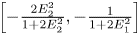
(i) $\boldsymbol K(s)$
is holomorphic in $\mathbb {C}\setminus {\left [-\frac {2E_2^{2}}{1+2E_2^{2}},-\frac {1}{1+2E_1^{2}}\right ]}.$(ii) $\frac {\boldsymbol K(s)-(\boldsymbol K(s))^{*}}{s-\overline {s}}\ge 0$
for all $Im{(s)}\ne 0$(iii) $\boldsymbol K(s)\ge 0 \text { for } \mathbb {R}\ni s>0$
because $s>0$ iff $\mathbb {R}\ni z>1$.


Then by the representation theorem in [Reference Dyukarev and Katsnelson20, theorem 3.1], there exists a monotonically increasing matrix-valued function $\pmb {\sigma }(t)$ , matrices $\pmb {A}\ge 0$
 and $\pmb {C}\ge 0$
 such that $\int _{+0}^{\infty } \frac {{\rm d}\pmb {\sigma }}{1+t}<\infty$
 , $\pmb {A}+\pmb {C}+\int _{+0}^{\infty } \frac {{\rm d}\pmb {\sigma }}{1+t}>0$
 and
and

As $s\rightarrow \infty$ , $z\rightarrow 1$
 and hence $\boldsymbol K\rightarrow \boldsymbol K(z=1)$
 . Therefore, we must have ${\pmb {C}=\pmb {0}}$
 . Moreover, $\pmb {A}=\boldsymbol K(s=0)=\boldsymbol K^{(D)}$
 . Also, since $\boldsymbol K(s)$
 is holomorphic in $\mathbb {C}\setminus {\left [-\frac {2E_2^{2}}{1+2E_2^{2}},-\frac {1}{1+2E_1^{2}}\right ]}$
 , we have

which is valid for all $s\in \mathbb {C}\setminus {\left [-\frac {2E_2^{2}}{1+2E_2^{2}},-\frac {1}{1+2E_1^{2}}\right ]}\subset (-1,0)$ . To compare with (3.14), which is valid only for $|s|>1$
 , we expand (3.17) near $s=\infty$
 to obtain the following series expansion

where $\boldsymbol {\mu }^{\sigma }_m$ is the $m$
 -th moment of the measure ${\rm d}\pmb {\sigma }$
 . Equating the coefficients term by term with (3.14) leads to the following relation between $\boldsymbol {\mu }^{\sigma }_m$
 and the ‘geometrical information’ coefficients in (3.15)


Recall that $\boldsymbol K$ can be regarded as a function of $s$
 as well as a function of $z$
 , $s:={1}/{(z-1)}$
 . In particular, the first moment $\boldsymbol {\mu }^{\sigma }_1$
 can be calculated explicitly as follows

4. Numerical verification
The computational domain with $Q=(0,1)^{2}$ , $Q_2=[1/4,3/4]^{2}$
 and $Q_1=Q\setminus Q_2$
 is illustrated in figure 2 and is chosen in the first two numerical examples, (4.1) and (4.2).

FIG. 2. Computational domain.
We consider three cases: (1) $Q_2$ is a solid obstacle, (2) $Q_2$
 is a bubble and (3) $Q_2$
 is another fluid.
For case (1), we find $(\mathbf{u}_1, p_1)\in \mathbf{V} _1 \times P_1$ , such that

where

For case (2), we find $(\mathbf{u}_2, p_2)\in \mathbf{V} _2 \times P_2$ , such that

where

For case (3), we set $\mu _1=1$ and $\mu _2=\mu$
 . We find $(\mathbf{u}_3, p_3)\in \mathbf{V} _3 \times P_3$
 , such that

where

The computation is done on square grids. The first level grid consists of 12 squares, for the first two cases. Each square is subdivided into 4 sub-squares to get the next level grid, $\mathcal {T}_h=\{T\}$ . We use the $Q_{5,4}^{1,0}\times Q_{4,5}^{0,1}$
 velocity finite-element space with the $Q_{4,4}^{0,0}$
 pressure finite-element space. Here $Q_{5,4}^{1,0}$
 means the space of polynomials of degree at most 5 in $y_1$
 and of degree at most $4$
 in $y_2$
 which is $C^{1}$
 in $y_1$
 -direction and $C^{0}$
 in $y_2$
 -direction. That is,

We note that $\mathrm {div} ( Q_{5,4}^{1,0}\times Q_{4,5}^{0,1}) = Q_{4,4}^{0,0}$ . Therefore, the finite element velocity is also pointwise divergence-free. We plot the velocity field of these two problems in figure 3. We can see the magnitude of the latter is much bigger, as the resistance from a slippery bubble is much less.


In figures 4 and 5, we plot the two velocity fields of two-fluid flow (4.3) for two viscosity coefficients $\mu _2$ . When $\mu _2$
 is big, the sticky inner fluid flows less and drags the outer fluid near the interface. When $\mu _2$
 approaches infinity, the inner fluid stops and it posts a zero Dirichlet boundary condition for on tangential velocity of the outer fluid at the inner boundary $\tilde \Gamma =\partial Q_2$
 . The model of a solid obstacle (4.1) is a limit case of the model of two-fluid (4.3) when $\mu _2\to \infty$
 . We can compare the left chart of figure 3 and the left chart of figure 4.

FIG. 4. Velocity field $\mathbf{u}_{3}$ for two-fluid flow (4.3) with $\mu _2=10^{2}$
 on $Q$
 (left), on $Q_2$
 (right, scaled by 200).

FIG. 5. Velocity field $\mathbf{u}_{3}$ for two-fluid flow (4.3) with $\mu _2=10^{-2}$
 on $Q$
 (left), on $Q_2$
 (right, scaled by 2).
When $\mu _2$ approaches zero, the inner fluid flow freely which produces little drag on the outer fluid. In theory, the force inside fluid $Q_2$
 may even push outer fluid somewhat. But due to the zero outflow boundary condition on the velocity at $\partial Q_2$
 , such a force would be balanced by its left portion and right portion of an edge of $\partial Q_2$
 . It is equivalent to zero tangential stress boundary on the outer flow. That is, model of a slippery bubble (4.2) is a limit model of two-fluid (4.3) with $\mu _2\to 0$
 . We may compare the right chart of figure 3 and the left chart of figure 5.
The homogenized permeability tensor $\boldsymbol K=\begin {pmatrix} k_{11} & k_{12}\\ k_{21} & k_{22} \end {pmatrix}$ is computed by


Due to the symmetry, in all our examples we have $k_{11}=k_{22}$ and $k_{12}=k_{21}=0.$
To verify the convergence results stated in (2.55) and (2.75), we solve the two-fluid problem (4.3) with $\mu _1=1$ and $\mu _2=10^{-4},\,1,\, 10^{4}$
 . In table I, this model is between the two ‘limiting’ models (4.1) and (4.2).


To see how viscosity $\mu _2$ influences the flow, we plot $(\mathbf{u}_{3})_1$
 in figure 6 for two different $\mu _2$
 with $\mu _1 = 1$
 .
.

FIG. 6. First component of velocity $\mathbf{u}_{3}$ , from (4.3), for $\mu =10^{2}$
 and $\mu _2=10^{-2}$
 .
.
Though the magnitude of $(\mathbf{u}_{3})_1$ is way larger than that of $(\mathbf{u}_{3})_2$
 , their corresponding stress are about the same size. In figure 7, we plot them for a comparison. We plot the stress intensity $|\nabla \mathbf {u}^{1}|$
 in figure 8.

FIG. 7. Stress $\nabla (u_{3})_1$ , and $\nabla (u_{3})_2$
 for (4.3) with $\mu _2=10^{2}$
 .
.

FIG. 8. Stress intensity $|e( (\mathbf{u}_3)_1 )|$ in (4.3) with $\mu _2=10^{2}$
 , $\mu _2=1$
 , $\mu _2=10^{-2}$
 .
.
Finally we compute the energy of the two-fluid flow,


The homogenized permeability can also be computed by the energy,

In table II, we demonstrate the equivalence of these two definitions for $k_{11}$ .
.
TABLE 2. Computed permeability $k_{11}$ both ways and energy

5. Conclusion and future work
In this paper, we show that the permeability of a porous material [Reference Tartar40] and that of a bubbly fluid [Reference Lipton and Avellaneda29] are limiting cases of the complexified version of the two-fluid models posed in [Reference Lipton and Avellaneda29]. We assume the viscosity of the inclusion fluid is $z\mu _1$ and the viscosity of the hosting fluid is $\mu _1$
 , $z\in \mathbb {C}$
 . The proof is carried out by construction of solutions for large $|z|$
 and small $|z|$
 by an iteration process similar with the one used in [Reference Bruno and Leo16, Reference Golden and Papanicolaou21] and analytic continuation. Moreover, we also show that for a fixed microstructure, the permeabilities of these three cases share the same IRF (3.17) with different values of $s$
 , as long as the ‘contrast parameter’ $s:={1}/{(z-1)}$
 is not in the interval $\left [-\frac {2E_2^{2}}{1+2E_2^{2}},-\frac {1}{1+2E_1^{2}}\right ]$
 , where the constants $E_1$
 and $E_2$
 are the extension constants that depend on the geometry of $Q_1$
 , $Q_2$
 and $Q$
 . For the mixture with bubbles, $s=-1$
 and thus

Also, we note that the matrix-valued measure in (3.10) has a Dirac measure sitting at $\lambda =0$ with strength equal to $\boldsymbol K^{(D)}$
 . The permeability $\boldsymbol K^{(D)}$
 is related to the measure in the sense that the zero-th moment of the measure is equal to ${\boldsymbol K(z=1)-\boldsymbol K^{(D)}}$
 .
.
Clearly, the positive matrix-valued measure ${\rm d}\pmb {\sigma }$ is independent of $s$
 and it characterizes how the geometry influences the permeability. We have shown that this measure is related to the projection measure of the self-adjoint operator $\Gamma _\chi$
 and its moments can be computed by equation (3.20).
Because the IRF is valid for most of $s$ on the complex plane, the IRF will be useful in the study of two-fluid mixture with complex viscosities such as dehomogenization for these fluid. Also, the integration limits in the IRF should imply bounds on the permeability tensors. We will explore the results of this paper in these direction in the future.
Acknowledgments
The work of CB and MYO was partially sponsored by the US National Science foundation via grants NSF-DMS-1413039 and NSF-DMS-1821857.


 Open access