


Introduction
Preferences for redistribution have increasingly received attention from political economy scholars (Alesina & Giuliano, Reference Alesina and Giuliano2011; Dimick et al., Reference Dimick, Rueda and Stegmueller2016, Reference Dimick, Rueda and Stegmueller2018; Dion & Birchfield, Reference Dion and Birchfield2010; Rueda, Reference Rueda2018; Rueda & Stegmueller, Reference Rueda and Stegmueller2019; Schmidt‐Catran, Reference Schmidt‐Catran2016). A crucial question in this topic relates to how citizens perceive the utility of redistribution. Do people perceive utility in absolute or relative terms, and are gains and losses perceived in the same way? This article develops a common framework showing how different attitudinal mechanisms operate side‐by‐side as a function of absolute and relative income distance from the mean income. Building on existing theories, I argue that gains from redistribution are perceived more in absolute terms while losses are perceived in relative terms. The analysis of cross‐national survey data from the Integrated Values Survey (IVS) finds that support for redistribution is determined by absolute income for the poor and relative income for the rich. This finding has important implications for distributive policies and political economy more broadly, suggesting that economic development makes public opinion less tolerant of income inequality.
Redistribution is the public transfer of economic resources across social groups, typically with the aim of reducing economic inequality. Redistributive policies usually take the form of tax and transfer programmes that grant net benefits to lower earners and impose net costs on higher earners. Governments – especially democracies but even autocracies – are accountable to (or at least constrained by) public opinion. People's attitudes influence how they vote, and – by extension – the policies that governments are driven towards enacting (Anderson & Beramendi, Reference Anderson and Beramendi2008, p. 12; Rueda & Stegmueller, Reference Rueda and Stegmueller2019, p. 8). Given rising levels of income inequality, understanding how those preferences form is a crucial first step towards knowing when governments are likely to enact redistribution.
Do people perceive the utility of redistribution in absolute or relative terms? And do they perceive gains and losses differently? These two questions lie at the heart of how redistribution preferences are formed. The literature is often agnostic about whether the utility of redistribution is perceived in absolute or relative terms. More importantly, though, it is commonly assumed that gains and losses are perceived equally, meaning that support for redistribution is monotonically determined by income position. However, this assumption has implications that are inconsistent with well‐established findings. If people perceive gains and losses equally and in absolute terms, then aggregate support for redistribution should be stable over time and independent of changes in levels of economic development or income inequality. This is because the utility of net gains is always matched by the utility of net losses. Income equalization implies transferring income from individuals above the mean (rich) to those below it (poor) until everyone's income is equal to the mean. Assuming that deadweight costs are evenly spread, the incomes gained by the poor should always be equal to the incomes that would be lost by the rich. If individuals value income in absolute terms and they value gains and losses equally, then the average utility of income equalization for a population would be zero: the positive utility of gains is matched by the negative utility of losses. This holds regardless of how much income there is in total or how it is distributed. However, studies show that support for redistribution varies substantially between and within countries over time and is affected by development and inequality (Andersen et al., Reference Andersen, Curtis and Brym2021; Beramendi & Rehm, Reference Beramendi and Rehm2016; Dion and Birchfield, Reference Dion and Birchfield2010; Lübker, Reference Lübker2007; Rueda, Reference Rueda2018). This means that some people display less self‐interest than others, depending on the context. In order to explain this variance, we must explore other mechanisms besides self‐interest.
This article contributes to the literature by making two important distinctions. First, it distinguishes between the absolute and relative utility of redistribution for individuals. Absolute utility is proxied by the absolute distance of an individual's income from the mean income, while relative utility is proxied by this same distance in relation to an individual's income. Second, it distinguishes between individuals who can expect net gains and net losses from redistribution. For this purpose, this article defines the poor and the rich as individuals with incomes below and above the mean, respectively. I hypothesize that the poor are more sensitive to absolute distance because they gain from redistribution, and the rich are more sensitive to relative distance because they lose from it. It is worth noting that this does not imply that people's preferences are sensitive to whether their income crosses the mean as a cutoff, but rather that their preferences become more sensitive to a different measure of income distance.
Four common concepts from the political economy literature explain why gains from redistribution are perceived in absolute terms and losses in relative terms: self‐interest, the diminishing marginal utility of income, inequity aversion and loss aversion. Self‐interest is the baseline mechanism that drives people to maximize their utility from redistribution (Meltzer & Richard, Reference Meltzer and Richard1981). The diminishing marginal utility of income means that the utility of additional income decreases as people get richer (Kaplow, Reference Kaplow2010). As a result, people's redistribution preferences are, to an extent, formed in relation to their current income, which serves as a reference point. Inequity aversion implies that people value positively reductions of income disparities (Fehr & Schmidt, Reference Fehr and Schmidt1999). This suggests that the rich display altruism in their preferences, since reducing inequality goes against their narrow material self‐interest. Meanwhile, loss aversion means that people weigh the value of losses more than the value of gains (Kahneman & Tversky, Reference Kahneman, Tversky, MacLean and Ziemba2013). In this context, loss aversion implies that the rich are more sensitive to relative changes because redistribution involves losses for them.
This article also makes a novel methodological contribution by estimating the household incomes of respondents to the IVS (the integration of the European Values Study (EVS) and the World Values Survey (WVS)), rather than using a scale or percentile measure of income. The main strengths of the IVS are its large size and cross‐national variance, which offer reliable and generalizable insights into public opinion. However, the item concerning respondents' incomes raises issues of comparability and interpretability because the surveys use different income scales and different currencies (Donnelly & Pop‐Eleches, Reference Donnelly and Pop‐Eleches2018). This problem is addressed here in two steps. First, I estimate respondents' income percentiles based on their rank within the distribution of the income scale for their survey. Second, I obtain their raw incomes by matching them to their corresponding country, year and income percentile in the World Income Inequality Database (WIID; UNU‐WIDER, 2021; Gradín, Reference n2021). This novel operationalization allows for a more precise and reliable estimation of raw income for IVS respondents and paves the way for future research concerning how income relates to both attitudes and socio‐demographic factors using one of the largest cross‐national survey datasets currently available.
Theory and hypotheses
In the political economy literature, redistribution preferences are generally viewed as being primarily determined by material self‐interest. The utility of redistribution can be defined as the net transfers an individual expects from income equalization. Since redistribution involves transferring incomes from people above the mean to those below it, taken to its logical conclusion, this eventually leads to all incomes being equalized. Therefore, the distance of a person's income from the mean income serves as a reliable proxy for the utility of redistribution. Indeed, self‐interest has been evidenced in numerous studies showing that the poor support redistribution more than the rich (Alesina & Giuliano, Reference Alesina and Giuliano2011; Andersen et al., Reference Andersen, Curtis and Brym2021; Bean & Papadakis, Reference Bean and Papadakis1998; Corneo & Grüner, Reference Corneo and Grüner2000; Dimick et al., Reference Dimick, Rueda and Stegmueller2016; Dion and Birchfield, Reference Dion and Birchfield2010; Finseraas, Reference Finseraas2009; Fong, Reference Fong2001; Gilens, Reference Gilens2005; Rueda, Reference Rueda2018).
Although self‐interest is arguably the primary driver of redistribution preferences, its influence is not uniform. Individual preferences are also shaped by other forces that can distort and countervail self‐interest, specifically the diminishing marginal utility of income, inequity aversion and loss aversion. Self‐interest implies that people seek to maximize their gains (and minimize their losses), so support for redistribution is determined by the absolute income distance. The diminishing marginal utility of income means that the utility of additional income units decreases as people get richer, which implies that people are conditioned by their income distance as a proportion of their current income. Inequity aversion means that people dislike inequality and want to reduce income disparities. For the poor, this simply leads to more self‐interest because they gain from reductions in inequality. But for the rich, this leads to altruism: they are willing to lose some income to reduce inequality. Lastly, loss aversion (the tendency to value losses more than gains) implies that the marginal utility of income diminishes more slowly when it involves losses, so the rich are more sensitive to relative utility than the poor.
Models of redistribution preferences are commonly based on the utility of what people expect to gain (or lose) from redistribution. Let series $x_i$ denote the income of individuals $i$ in a population of size $n$. The mean income is defined as $\bar{x}=\frac{1}{n}{\sum}_{i=1}^{n}{x}_{i}$. The utility of redistribution can then be described as the distance of a person's income from the mean, which can be formulated in absolute $(\bar{x}-x_i)$ or relative terms $(\bar{x}-x_i)/x_i$. This distinction is exemplified in Table 1, showing a series of incomes for Country A and Country B. Equation (1) formulates the utility of redistribution allowing gains and losses to be valued differently. Here, $\alpha$ represents the value given to absolute utility and $\beta$ for relative utility. Positive distances indicate gains ( $g$), while negative ones indicate losses ( $l$).
$l$).
 $$\begin{equation} u(x_i, \alpha, \beta)= {\begin{cases} \alpha _g(\bar{x}-x_i)+\beta _g(\bar{x}-x_i)/x_i & \text{ if } x_i < \bar{x}\\ \alpha _l(\bar{x}-x_i)+\beta _l(\bar{x}-x_i)/x_i & \text{ if } x_i > \bar{x} \end{cases}}. \end{equation}$$
Table 1. Examples of income series with absolute and relative income distance

Under pure self‐interest, preferences would be determined solely by the absolute distance ( $\alpha >0$ and $\beta =0$), and gains and losses would be treated the same ( $\alpha _g=\alpha _l$). As a result, average utility would always be zero because the total value of absolute gains is equal to that of losses. In other words, the positive utility that the poor gain from redistribution is matched by the negative utility that the rich lose from paying taxes: $\sum ^{n}_{i=1}{\bar{x}-x_i}=0$. Assuming that self‐interest makes redistribution preferences monotonically proportional to the expected returns from income equalization, then average support for redistribution should be static across contexts and time and independent of changes in development or inequality. However, if people value gains and losses differently – or perceive utility in relative terms – this would explain shifts in public demand for redistribution. As explained below, inequity aversion means that preferences are less sensitive to absolute losses ( $\alpha _g>\alpha _l$), and loss aversion means that preferences are more sensitive to relative losses ( $\beta _g>\beta _l$).
Self‐interest
Material self‐interest serves as the most common basis for understanding individuals' preferences for redistribution. The principles behind this idea can be traced back to rational choice theory (Downs, Reference Downs1957) and social choice theory (Arrow, Reference Arrow1974; Arrow & Debreu, Reference Arrow and Debreu1954). The most popular version of this approach is the one proposed by Romer (Reference Romer1975) and developed by Meltzer and Richard (Reference Meltzer and Richard1981), the Romer–Meltzer–Richard (RMR) model. Its central proposition is that people seek to maximize their own material well‐being: the more people expect to gain (lose) from redistribution, the more (less) they support it.
In theory, utility‐maximizing material self‐interest would dictate that all people below the mean would want a 100 per cent tax rate so that all incomes were equal. Conversely, those above the mean would want a tax rate of zero in order to keep all of their income. Nonetheless, there are reasons we would expect rational self‐interested people to respond gradually to income disparities, rather than maximally (i.e., preferences should not shift from one extreme to the other in response to small incentives). Changes in the distribution of incomes can entail unintended consequences that offset its utility, leading to deadweight costs (e.g., more redistribution stymieing economic growth or less redistribution leading to more crime and social unrest). Additionally, preferences can be conditioned by distortionary costs (e.g., people being unaware of how policies would affect them or not even knowing their own position in the income distribution).
Assuming that the costs and benefits of redistribution are spread uniformly across the population or as a proportion of income, preferences should be monotonically determined by income distance according to the RMR model. This will never be exactly the case, of course. Some redistributive policies may be more targeted (e.g., giving to the poorest or taxing the richest), while others may be more generalized (e.g., giving to most people below the mean or taxing most people above it). Furthermore, tax and transfer programmes may or may not be proportional to income (e.g., the richest giving to all the poor or all the rich giving to the poorest). Still, if we conceptualize redistribution as policies that aim to bring us closer to income equalization, we can understand redistribution preferences as the extent to which people support or oppose this. Thus, the first hypothesis contends that absolute income distance determines support for redistribution because it reflects the absolute utility expected from income equalization.
Hypothesis 1: There is a negative relationship between individuals' absolute income distance and their support for redistribution.
Within the framework of self‐interest, current income is not the only relevant factor. The extent to which redistributive policies will benefit a person also depends on their prospects for future income as well as notions of risk and insurance. According to the ‘life‐cycle hypothesis’ (Modigliani et al., Reference Modigliani and Brumberg1954), people tend to have less income when they are younger and older. Moreover, a person's education and occupational status influence how their income evolves during their life (Alt & Iversen, Reference Alt and Iversen2017; Iversen & Soskice, Reference Iversen and Soskice2001; Rehm, Reference Rehm2009, Reference Rehm2016). People with higher educational attainment tend to have lower incomes while they are students but can expect higher and more stable earnings over their lifetime. A country's existing welfare policies also influence preferences: generous safety nets and strong unionization provide insurance for incomes. Lastly, social mobility also conditions the prospects of future income. People on the lower end of the income distribution are often apprehensive about redistributive policies when they believe in their prospects for upward mobility (Feldman & Zaller, Reference Feldman and Zaller1992; Lipset & Bendix, Reference Lipset and Bendix1991; Manza & Brooks, Reference Manza and Brooks2021).
Diminishing marginal utility of income
As a person's income increases, the additional utility from each additional unit of income decreases. For example, going from $100 to $200 adds more relative utility than going from $1000 to $1100. Even though the absolute utility is +$100 in both cases, it implies a 100 per cent increase in the first case but only a 10 per cent increase in the second case. This means that the utility of income follows a concave function. The diminishing marginal utility of income has long been used to explain why the rich tolerate progressive taxation (Atkinson, Reference Atkinson, Parkin and Nobay1973; Bakija & Slemrod, Reference Bakija and Slemrod2004; Blackorby et al., Reference Blackorby, Bossert, Donaldson and Silber1999; Kaplow, Reference Kaplow2010; Mirrlees, Reference Mirrlees1971; Slemrod et al., Reference Slemrod, Yitzhaki, Mayshar and Lundholm1994; Stein, Reference Stein1991; Stern, Reference Stern1976; Tuomala, Reference Tuomala1990). As Kaplow (Reference Kaplow2010) writes, ‘concavity of individuals’ utility functions may well be the dominant determinant of the magnitude of the social preference for equalizing incomes' (p. 39).
Research on redistribution preferences often takes into account this phenomenon. Some studies estimate the effect of absolute income distance under specifications that allow for a curvilinear relationship, thus introducing concavity (Dimick et al., Reference Dimick, Rueda and Stegmueller2016; Rueda & Stegmueller, Reference Rueda and Stegmueller2019). Dion and Birchfield (Reference Dion and Birchfield2010) measure income distance in terms of the standard deviation of incomes for a given country‐year, so the same values indicate larger absolute income distances depending on how rich the population is. The effects of absolute and relative utility, though, have not been examined side‐by‐side in previous studies.
To the extent that people's preferences are determined by their relative – as opposed to absolute – distance from the mean income, those preferences reflect the concavity of income utility. In Equation (1), $\beta$ is the parameter for relative utility. If people were sensitive only to their relative income distance ( $\alpha =0$ and $\beta >0$), they would not care about how much they gained or lost from redistribution, but rather what they gained or lost as a proportion to their current income. Based on the diminishing marginal utility of income, the second hypothesis contends that support for redistribution is determined by relative income distance. People are more likely to support changes in the distribution of incomes when the benefits have a meaningful positive impact on their life compared to their current state of affairs. The more people gain from redistribution in relation to their income, the more they are likely to support it.
Hypothesis 2: There is a negative relationship between individuals' relative income distance and their support for redistribution that is independent of the effect of absolute income distance.
Altruism and inequity aversion
Altruism is the opposite of self‐interest: when a person ‘is willing to sacrifice own resources in order to improve the well‐being of others’ (Fehr & Schmidt, Reference Fehr and Schmidt2006, p. 620). Formal theories on altruism were pioneered in the fields of behavioural economics and game theory (Andreoni & Miller, Reference Andreoni and Miller1995; Bolton & Ockenfels, Reference Bolton and Ockenfels2000; Dufwenberg & Kirchsteiger, Reference Dufwenberg and Kirchsteiger2004; Falk & Fischbacher, Reference Falk and Fischbacher2006; Fehr & Schmidt, Reference Fehr and Schmidt1999; Levine, Reference Levine1997; Rabin et al., Reference Rabin1992) and have subsequently been applied to redistribution preferences (Cavaille, Reference Cavaille2014; Cavaillé & Trump, Reference Cavaillé and Trump2015; Dimick et al., Reference Dimick, Rueda and Stegmueller2016, Reference Dimick, Rueda and Stegmueller2018; Lupu & Pontusson, Reference Lupu and Pontusson2011; Rueda, Reference Rueda2018; Rueda & Stegmueller, Reference Rueda and Stegmueller2019). In its unconditional form, altruism would imply not only that the rich want to give more money to the poor but also that the poor want to let the rich keep their money. In the context of redistribution, though, altruism is of course viewed as affecting preferences conditionally, depending on whether people are above or below the mean income, to explain why the rich display less self‐interest.
Conditional altruism among the rich is commonly attributed to ‘inequity aversion’ (or difference aversion): ‘an individual is inequity averse if he dislikes outcomes that are perceived as inequitable’ (Fehr & Schmidt, Reference Fehr and Schmidt1999, p. 820). Inequity aversion implies that people value payoffs to others more positively if those payoffs reduce disparities (Daughety, Reference Daughety1993; Fehr & Schmidt, Reference Fehr and Schmidt1999; Fehr et al., Reference Fehr, Kirchsteiger and Riedl1998). So a person whose income is above the mean will value payoffs to others more positively than those with incomes below it: inequity aversion drives altruism among the rich and self‐interest among the poor. There is ample empirical evidence for inequity aversion: experimental studies show that people prefer more equal economic allocations, even if it comes at the cost of their own payoffs (Aguiar et al., Reference Aguiar, Hurst and Karabarbounis2013; Charité et al., Reference Charité, Fisman, Kuziemko and Zhang2022; Charness & Rabin, Reference Charness and Rabin2002; Klor & Shayo, Reference Klor and Shayo2010).
Observational studies provide implicit evidence of altruism, either by estimating aggregate effects in support of redistribution or by identifying moderating factors that enhance altruism among the rich. Many studies show that public opinion is more favourable to social spending in affluent countries (Alt, Reference Alt1979; Blomberg & Kroll, Reference Blomberg and Kroll1999; Rose & Peters, Reference Rose and Peters1978; Sealey, Reference Sealey2018; Stevenson, Reference Stevenson2001), implying that people become more altruistic as they become richer. Summarizing this view, Rapoport and Vidal (Reference Rapoport and Vidal2007) write that ‘once individuals have satisfied their own physiological constraint in the course of economic development, they devote resources to shaping their altruistic preferences, increasing their social degree of altruism above its natural level’ (p. 1231). In particular, the rich become more altruistic in cases of high inequality and ethnic homogeneity (Cavaillé & Trump, Reference Cavaillé and Trump2015; Rueda, Reference Rueda2018; Rueda & Stegmueller, Reference Rueda and Stegmueller2019).
Although previous studies show factors that enhance altruism driven by inequity aversion, they do not outright estimate the difference in self‐interest between the rich and the poor. This study aims to directly estimate levels of altruism by comparing the effect of absolute income distance for the rich and the poor in their redistribution preferences. Thus, the third hypothesis contends that inequity aversion drives altruism among the rich.
Hypothesis 3: The negative effect of income distance on support for redistribution is weaker among individuals with incomes above the mean.
Altruism implies that the absolute utility parameter is lower for the rich than for the poor. In Equation (1), $\alpha _g$ and $\alpha _l$ indicate the utility of absolute gains and losses, respectively. These parameters reflect how self‐interested the poor and the rich are compared to each other: $\alpha _g>\alpha _l$ would indicate that people are altruistic (i.e., value positively the utility of others who are worse off), and $\alpha _g<\alpha _l$ would indicate spite (i.e., people value negatively the utility of others who are worse off). Thus, the level of altruism (or spite) can be measured by the difference in utility perceived from gains and losses.
Loss aversion
Just as pure self‐interest would imply that absolute gains and losses are perceived equally, the diminishing marginal utility of income by itself would imply that relative gains and losses are perceived the same way. In other words, that the marginal utility of income diminishes at a constant rate. However, loss aversion implies that people perceive the marginal utility of income as higher when it involves losses. Conversely, if people were gain‐seeking, they would value income more when it involves gains. These concepts can explain why the effect of relative income distance on support for redistribution is different for the rich and the poor.
As Kahneman and Tversky (Reference Kahneman, Tversky, MacLean and Ziemba2013) note, ‘individuals normally perceive outcomes as gains and losses, rather than as final states of wealth or welfare’ (p. 274); more succinctly, ‘losses loom larger than gains’ (p. 279). The extent to which people are loss averse is reflected in the size of the concave kink of a gain–loss utility function in relation to a reference point (Köbberling & Wakker, Reference Köbberling and Wakker2005). A higher concavity for the utility of losses indicates that people are more loss averse. This concept has been integrated into models of social choice, including redistribution preferences. Benjamin (Reference Benjamin2015) develops a model that defines utility according to relative changes in income, arguing that people are loss‐averse over changes in their payoffs. This explains why it is often considered unfair for landlords to raise rents for existing tenants, but fair to raise rents for new ones. Alesina and Passarelli (Reference Alesina and Passarelli2019) also use loss aversion to explain institutional tendencies towards policy entrenchment and moderation.
In the context of redistribution, loss aversion implies that the rich are more sensitive to relative distance because the marginal utility of income is higher when it involves losses. This means that the same difference in overall income level is valued more when moving downward: going from $20,000 to $10,000 is perceived more negatively than going from $20,000 to $30,000 is positive. There is experimental evidence for this phenomenon. Charité et al. (Reference Charité, Fisman, Kuziemko and Zhang2022) explore how reference points and loss aversion shape redistribution preferences, finding that agents who are assigned the role of social planners redistribute much less from rich to poor when the subjects are aware of the initial endowments. The authors claim that redistributors consider the loss experienced by the rich as larger than the benefits enjoyed by the poor.
While the diminishing marginal utility of income suggests that redistribution preferences are determined by the relative distance to the mean, loss aversion implies that the same relative distance is perceived more strongly when it involves losses. In Equation (1), $\beta _g$ and $\beta _l$ indicate the value of relative gains and losses, respectively, so loss aversion is reflected in the extent to which the utility of relative losses is larger than the utility of relative gains ( $\beta _l>\beta _g$). (Conversely, if people were gain‐seeking, the poor would be more sensitive to relative distance.) Thus, the fourth hypothesis contends that the rich are more sensitive than the poor to the relative utility of redistribution due to loss aversion.
Hypothesis 4: The negative effect of relative income distance on support for redistribution is stronger among individuals with incomes above the mean.
Data and methods
Sample
To test the hypotheses, this study uses the IVS (the integration of the WVS and the EVS), a pooled cross‐sectional time‐series dataset of cross‐national surveys of weighted representative samples of about 1500 respondents starting from 1981 (EVS, Reference EVS2021; Inglehart et al., Reference Inglehart, Haerpfer, Moreno, Welzel, Kizilova, Diez‐Medrano, Lagos, Ponarin and Puranen2020). This dataset includes attitudinal and socio‐demographic data that allow for a comparative analysis of the relationship between people's economic attitudes and their income position. The original sample consists of 652,990 respondents in 455 surveys of 117 countries,Footnote 1 and the final sample without missing data consists of 478,865 respondents in 372 surveys of 103 countries.Footnote 2
Support for redistribution
The dependent variable in the analysis is individual‐level support for redistribution, measured by the ‘Income Equality’ question from the IVS surveys (Item E035), which uses a 10‐point scale on which 1 indicates support for less redistribution and 10 indicates support for more redistribution. The item is worded as followsFootnote 3:
How would you place your views on this scale? (1) We need larger income differences as incentives. (10) Incomes should be made more equal.
This question has been used as the outcome variable in numerous studies (Ansell & Samuels, Reference Ansell and Samuels2010; Hayward & Kemmelmeier, Reference Hayward and Kemmelmeier2011; Iglesias et al., Reference Iglesias, López and Sántos2013; Pepinsky & Welborne, Reference Pepinsky and Welborne2011) as have other questions about specific economic issues like business ownership (Bjørnskov & Paldam, Reference Bjørnskov and Paldam2012) and individual responsibility to provide (Andersen et al., Reference Andersen, Curtis and Brym2021; Sealey, Reference Sealey2018). The distribution of support for redistribution is displayed in Figure A1 in the online Appendix, and the distributions (and means) for each country‐year survey are shown in Figure A4 in the online Appendix.
Patterns observed from such cross‐national datasets are generalizable, given that each survey asks the same question across different countries. Other surveys like the European Social Survey (ESS) and the International Social Survey Programme (ISSP) include similar items (asking whether respondents believe that the government should reduce income differences) using 5‐point Likert scales. I use the IVS for two main reasons. First, the IVS offers a wider breadth of cross‐national coverage‐over 100 countries, compared to the 35 and 45 of the ISSP and ESS, respectively. Second, the 10‐point scale of the IVS provides more variance and a less skewed distribution than the 5‐point scales of the other surveys, as is shown in Figures A1–A3 in the online Appendix. Survey questions with 10‐point scales have been found to have advantages over those with 5‐point scales because they have higher convergent and discriminant validity while maintaining similar means (Coelho & Esteves, Reference Coelho and Esteves2007).
One complication with surveying people's preferences towards redistribution is that redistributive policies can take different forms. Some policies focus on tax and transfer programmes directly involving people's income, while others involve public spending on welfare state programmes or public services for the general public that happen to have net redistributive effects. Studies have also differentiated between policies that focus on taxing the rich more and policies that focus on transferring more to the poor (Cavaillé & Trump, Reference Cavaillé and Trump2015; Sealey, Reference Sealey2018). Policies may increase taxes on a narrow segment of high earners and transfer income to a broad segment of low earners or vice versa. As the survey questions do not specify who should pay/receive income transfers or how large the transfers should be, we can generally conceive of these questions as alluding to a generic notion of income equalization whereby incomes are redistributed in a way that is proportional to income and symmetric around the mean.
It is also worth noting that these questions are normally framed in relation to the current state of affairs. Respondents are asked whether the government should do more or less to reduce income disparities, rather than what the ideal distribution of incomes would be.Footnote 4 As a result, respondents are likely to answer the question in relation to how they perceive current levels of inequality, and they may also take into account existing levels of redistribution. As Schmidt‐Catran notes (Reference Schmidt‐Catran2016, p. 126), respondents could understand these questions in relation to what the government is already doing to ameliorate inequality. If social spending is already high, people may be less likely to support increases.
Clearly, we need to interpret cautiously any patterns found in these responses. Models predicting responses to these questions must account for existing levels of income inequality. Although social spending is also relevant, data on it tend to be less available and less comparable (what counts as social spending can be disputed and can vary across countries). Moreover, the effects of social spending should eventually spill over to levels of inequality. Even in cases where inequality is high despite large social spending, it is ultimately the distribution of incomes that determines the pool of resources that are available for redistribution.
Absolute and relative income distance
The two main independent variables of the analysis are absolute income distance (mean income minus income) and relative income distance (income distance divided by income). Both variables are based on respondents' net household income and their country's mean income, which is equivalent to GDP per capita. These independent variables are operationalized by combining the IVS survey data with the WIID,Footnote 5 which collects annual data from different sources on the income distribution of countries, as well as GDP per capita PPP (purchasing power parity) in 2017 international dollars and Gini estimates (see Gradín, Reference n2021). The operationalization of household income consists of two steps: first, I estimate respondents' income percentile from the IVS question on income scales; second, I obtain respondents' household income by matching their income percentile with the WIID dataset.
The IVS includes a ‘Scale of Incomes’ question (Item X047) that uses country‐specific household income scales labelled in national currency, employs 10 categories (10 per cent lowest to 10 per cent highest income category) and is worded as followsFootnote 6:
Here is a scale of incomes, and we would like to know in what group your household is, counting all wages, salaries, pensions and other incomes that come into, after taxes and other deductions. (1) First step, (10) Tenth step.
While the cutoffs for the steps vary across countries and sometimes even across surveys of the same country, this item can still be used to rank respondents according to the distribution of responses for their particular country‐year survey (Donnelly & Pop‐Eleches, Reference Donnelly and Pop‐Eleches2018). Each respondent is assigned a percentile value (1–100) based on their income position relative to the rest of respondents. Based on the share of respondents that selected each step, they are assigned the percentile value of the median cumulative share for their step. This maximizes the variance of respondents' incomes without biasing the variable. The distributions of responses to the item on income scales for each survey are illustrated in Figure A5 in the online Appendix.
Once the income percentile of IVS respondents is estimated, I obtain their net household income using the WIID, which uses the Shorrocks–Wan approach (Shorrocks & Wan, Reference Shorrocks and Wan2008) to produce synthetic distributions of net household incomes (after tax and transfers) at the country‐year level that describes the estimated income for each percentile group (see Gradín, Reference n2021). Respondents are then assigned the net household income corresponding to the country, year and income percentile in the WIID. Joining IVS survey data with the WIID dataset by income percentile provides a reliable and comparable estimate of how much money each respondent makes.
The process for obtaining respondents' raw income is shown in Figure 1 and Table 2 using the example of the survey of Spain in 2008. As we can see, the share of respondents who fall into each category is hardly constant: 20 per cent place themselves in the 4th step, but only 5 per cent in the 10th. The cumulative share corrects this by indicating where each group of respondents falls in relation to the sample as a whole. For example, 96 per cent of respondents placed themselves in or below the 9th step, so we know that the respondents who picked the 10th step represent the top 4 per cent of respondents. Each group is then assigned the income percentile equivalent to the middle of the range of the cumulative share corresponding to the income step they selected. For example, the respondents who picked the 4th step fall between the 14th and the 33rd percentiles, so they are assigned the 24th percentile.

Figure 1. Histogram of responses for “Income Scales” (Item X047) of IVS for Spain in 2008.
Table 2. Responses for “Income Scale” (Item X047) in the IVS for Spain in 2008

Note: Income step indicates response to the ‘Income Scale’ question. Freq. (Frequency) indicates the number of respondents who placed themselves in the income step. Share indicates the weighted share of respondents who placed themselves in the income step. Income percentile is the average income percentile that can be imputed to each income group. Income is the estimated net household income in the WIID for the corresponding country, year and income percentile. Mean income is the average income for the country‐year in the WIID. Income distance is income minus the mean income. Relative income distance is the absolute income distance divided by income.
This method maximizes the variance that can be extracted from the responses while keeping the measure of income percentile unbiased. The strength of this approach is that it will not yield biased measurements even if respondents give biased answers. For example, assuming that the scales used in the survey for Spain in 2008 were accurate (each scale representing one decile) and the sample was representative, it is clear that the poorest respondents overestimated their place on the income distribution and the richest ones underestimated it. Although this reduces the variance of the measure, the resulting ranks are still accurate because they compare respondents to the distribution of responses (even if the bias of respondents is correlated with their income position).
Finally, respondents' absolute and relative income distances are calculated from their income and the mean income for their corresponding country‐year, which is equivalent to GDP per capita.Footnote 7 Continuing the example of the survey of Spain in 2008, Table 2 shows the income distance corresponding to each group from the income scale item. Absolute income distance is calculated as the mean income minus respondents' income. Since the GDP per capita of Spain in 2008 was $\$39,286$, the absolute income distance is $+\$32,602$ for respondents who selected 1 on the Income Scale and $-\$64,132$ for those who selected 10. Relative income distance is operationalized as respondents' absolute income distance divided by their income. Thus, a value of $+1.00$ indicates that a respondent's income is half of the mean, and a value of $-0.50$ indicates that it is double. In the example from Table 2, the relative income distance is $+4.88$ for respondents who selected 1 on the Income Scale because income equalization would increase their income by 488 per cent, and $-0.62$ for respondents who selected 10 because they would lose 62 per cent of their income. The scatterplot in Figure 2 shows how absolute and relative income distances are distributed in relation to each other.

Figure 2. Scatterplot of absolute and relative income distance in the IVS with histograms.
Controls
Various socio‐demographic characteristics are used as controls in the analyses due to the potential endogeneity they might create between income and redistribution preferences: gender, age, marital status, having children, employment status, religiosity and political trust. (Education and urbanization are added as controls later due to higher missing rates in the IVS.) The IVS includes questions for these variables, and their operationalization is outlined in the online Appendix. Previous studies of WVS data show that support for redistribution is associated with older respondents, women, lower educational attainment and marriage (Alesina & Giuliano, Reference Alesina and Giuliano2011; Attewell, Reference Attewell2022). Numerous studies have also linked religiosity to less support for redistribution (Brammer et al., Reference Brammer, Williams and Zinkin2007; Guiso et al., Reference Guiso, Sapienza and Zingales2003; Renneboog & Spaenjers, Reference Renneboog and Spaenjers2012; Stegmueller, Reference Stegmueller2013). The analyses also control for levels of income inequality for the country‐year of the survey, to account for differences in preferences for redistribution that are based on national considerations rather than individual ones. Income inequality is measured using the Gini coefficient, also obtained from the WIID.
Analysis
The main analysis consists of generalized linear mixed‐effects models predicting respondents' support for redistribution. The models assess the independent effects of each component while accounting for control variables. Since the dataset has a multilevel structure (individual respondents are nested in country‐year surveys nested in countries), I use mixed‐effects models containing both fixed and random effects to address potential complications (clustering, nonconstant variance, underestimation of standard errors, etc.). This type of model has been proposed for studies of pooled cross‐sectional time‐series datasets like the IVS (Fairbrother, Reference Fairbrother2014; Schmidt‐Catran & Fairbrother, Reference Schmidt‐Catran and Fairbrother2016) and has been employed in similar studies (Fairbrother, Reference Fairbrother2013, Reference Fairbrother2016; Rueda, Reference Rueda2018; Schmidt‐Catran, Reference Schmidt‐Catran2016; Sealey, Reference Sealey2018). The analysis uses random effects (RE) models over fixed effects (FE) models because they can include random slopes that account for group‐level variance in the relationship between variables (for a review, see Bell et al., Reference Bell, Fairbrother and Jones2019). Since FE models do not account for this, it can lead to biased estimates and anti‐conservative standard errors. As Bell et al. (Reference Bell, Fairbrother and Jones2019) write, ‘in most research scenarios, a well‐specified RE model provides everything that FE provides and more, making it the superior method for most practitioners’ (p. 1052). A potential drawback of RE models is that they assume that random effects are drawn from a normal distribution, which can lead to a ‘modest bias’ when this is not the case (Bell et al., Reference Bell, Fairbrother and Jones2019, p. 1051). For this reason, the models are replicated using FE models as a robustness check.
The RE models include random effects by country and country‐year to account for differences across countries and time. This implies that the effects of country and country‐year are drawn from a common normal distribution with estimated variance. The heterogeneity of effects can influence support for redistribution as well as the effect that income has on support. The random effects include random intercepts and random slopes for the explanatory variables (i.e., absolute and relative income distance, the rich/poor discontinuity and their interactions). Random intercepts by country capture differences that are due to enduring factors such as culture, region or majority religion (Andersen et al., Reference Andersen, Curtis and Brym2021; Dion and Birchfield, Reference Dion and Birchfield2010; Lübker, Reference Lübker2007), and random intercepts by country‐year capture changes in factors such as economic conditions. Random slopes capture systemic differences in the relation between attitudes and the variables of interest. For example, historical background can be a potential source of endogeneity between public opinion and social policy: countries with communist legacies have been associated with economic stagnation (Benjamin & Kautsky, Reference Benjamin and Kautsky1968; Crafts & Toniolo, Reference Crafts and Toniolo2010; Harrison, Reference Harrison2012) and weaker economic political cleavages (Gijsberts & Nieuwbeerta, Reference Gijsberts and Nieuwbeerta2000; Loveless & Whitefield, Reference Loveless and Whitefield2011; Rohrschneider & Whitefield, Reference Rohrschneider and Whitefield2009; Saarts, Reference Saarts2016).
Results
The main argument outlined in the theory is that preferences for redistribution are shaped by whether people can expect to gain or lose from it, with gains being perceived in absolute terms and losses in relative terms. To test the hypotheses derived from this argument, I report on the effects of absolute and relative income distance on respondents' support for redistribution, conditional on whether their income is below or above the mean. Table A2 in the online Appendix shows the means, standard deviations and intercorrelations of all variables. Support for redistribution has positive correlations with absolute income distance ( $\beta = 0.09$, $p < 0.001$) and relative income distance ( $\beta = 0.04$, $p < 0.001$), confirming that respondents who are richer are indeed less supportive of increasing redistribution. Figures 3 and 4 show the relationship between income distance and support in more detail. Figure 3 illustrates general additive models of these relationships, and Figure 4 displays the slopes from simple ordinary least squares (OLS) regressions for the rich and poor in each country‐year survey in the IVS.Footnote 8 Support for redistribution is shown to be more closely associated with positive absolute distance and negative relative distance, providing initial support for a discontinuous relationship around the mean income.

Figure 3. Ordinary least squares trendlines of support for redistribution by absolute and relative income distance with discontinuity at the mean income.

Figure 4. Generalized additive models of support for redistribution by absolute and relative income distance with discontinuity at the mean income.
Table 3 reports the results of the generalized mixed‐effects models, which include controls and random effects by country and country‐year. The models show the effects of absolute and relative income distance conditional on the discontinuity based on the cutoff around the mean (i.e., poor or rich). Meanwhile, Table 4 shows the results using split‐sampling (separate analyses of subsamples of poor and rich respondents) instead of discontinuous interactions, making them easier to interpret.
Table 3. Generalized linear mixed‐effects models predicting support for redistribution

Notes: Controls include year (1980 = 0), Gini, employment status, gender, age, marital status, children, religious attendance and political trust. Random effects include random intercepts and random slopes for rich and absolute and relative income distance (when included) by country and country‐year. $\chi ^2$ for Model 1 is compared to a model that only includes controls.
Significance: *p $<$ 0.05; **p $<$ 0.01; ***p $ <$ 0.001.
Table 4. Generalized linear mixed‐effects models predicting support for redistribution with split‐sampling by poor/rich

Notes: Controls include year (1980 = 0), Gini, employment status, gender, age, marital status, children, religious attendance and political trust. Random effects include random intercepts and random slopes and absolute and relative income distance (when included) by country and country‐year. $\chi ^2$ for Models 1A and 1B are compared to a model that only includes controls.
Significance: *p $<$ 0.05; **p $<$ 0.01; ***p $<$ 0.001.
The results from Model 1 show support for H1: absolute income distance has a significant positive effect on support for redistribution ( $\beta = 0.222$, $p < 0.001$). This means that there is an estimated difference of 0.44 points between two people with incomes that are $\$10,000$ above and below the mean. Moreover, the chi‐squared of Model 1 ( $\chi ^2 = 4775.7$, $p < 0.001$) is statistically significant and far larger than that of the control model ( $\chi ^2 = 2445.0$, $p < 0.001$), indicating that income distance has substantially more explanatory power than the controls, as one would expect given that it is a proxy for respondents' utility from redistribution. This finding is consistent with extant research on the RMR model, which holds that preferences for redistribution are driven by absolute utility.
The results from Model 2 provide support for H2, showing that relative income distance also has a significant positive effect ( $\beta = 0.084$, $p < 0.001$), even when accounting for absolute income distance. There is an estimated difference of 0.17 points between individuals with relative income distances of − $0.50$ and $1.50$ (i.e., a person making twice the mean income and a person making two‐thirds the mean income). Moreover, the chi‐squared of Model 2 ( $\chi ^2 = 941.6$, $p < 0.001$) is statistically significant, indicating that relative distance adds explanatory power. This finding is consistent with the notion that income has a diminishing marginal utility, suggesting that while preferences for redistribution are motivated by self‐interest, they are also shaped by how much money a person already makes.
The next hypotheses, H3 and H4, argued that preferences for redistribution are not only determined by absolute and relative utility, but that these effects differ between those who gain and those who lose from redistribution. The effect of absolute distance is hypothesized to be weaker for the rich because of inequity aversion (H3), and the effect of relative distance is hypothesized to be stronger for the rich because of loss aversion (H4). To address these claims, I turn to the discontinuous effects of absolute and relative income distance. Before doing so, it is worth noting that the inclusion of the discontinuous effects based on the rich/poor cutoff adds explanatory power for both absolute ( $\chi ^2 = 631.7$, $p < 0.001$) and relative income distance ( $\chi ^2 = 252.9$, $p < 0.001$).
Model 3 shows support for H3, as the interaction of absolute income distance with above‐mean income is significantly negative ( $\beta = -0.219$, $p < 0.001$), meaning that absolute income distance has a weaker effect on the rich. This is displayed more clearly in the split‐sample results from Table 4: the effect of $\$10,000$ in absolute distance is 0.37 points for the poor, but only 0.02 points for the rich (Models 1A and 1B). The asymmetry in the effect of absolute income provides evidence of inequity aversion, as it indicates that people below the threshold of equal distribution display more self‐interest and those above display altruism.
Model 4 shows support for H4, as the interaction of relative income distance with above‐mean income is significantly positive ( $\beta = 0.686$, $p < 0.001$), suggesting that the rich are more sensitive to relative income distance. In the split‐sample models, a relative distance of $10 {\rm per cent}$ affects support by 0.07 points for the rich, while the effect is negligible for the poor (Models 2A and 2B). This provides evidence for loss aversion because it means that the marginal utility of relative changes in income is larger for the rich.
The effect of the dichotomous rich/poor variable is worth highlighting, as it reflects the effect of crossing the mean income threshold. While absolute and relative income distance have meaningful discontinuous effects, the dichotomous rich/poor variable is not significant in Model 4. This suggests that crossing the mean income threshold by itself does not affect redistribution preferences. Rather, respondents are more sensitive to absolute or relative utility depending on whether they are poor or rich.
To illustrate these effects, I estimate predicted levels of support for redistribution by setting the variables of interest to chosen values while holding all other variables to the mean. Figure 5 presents the predicted values (with $95 {\rm per cent}$ confidence intervals) for absolute income distance ranging from $-\$40,000$ to $+\$20,000$ and relative income distance ranging from $-60 {\rm per cent}$ to $+300 {\rm per cent}$ (the bottom/top $10 {\rm per cent}$ ranges for the poor/rich). The results show how absolute distance has a significant effect only for the poor, while relative distance has a significant effect only for the rich. As absolute income distance rises from $\$0$ to $\$20,000$, estimated support rises 0.66 points (5.10–5.75), but as it drops from $\$0$ to $-\$40,000$, estimated support does not change significantly. Meanwhile, as relative income distance drops from $0.00$ to $-0.60$, estimated support drops 0.41 points (5.07–4.66), but as it rises from $0.00$ to $3.00$ there is no significant change in support. These discontinuous effects provide evidence that the poor base their preferences on the absolute utility of redistribution, while the rich base theirs on relative utility.

Figure 5. Predicted support for redistribution based on absolute and relative income distance (Table 3 Model 4).
These results can also be disaggregated by individual‐level income and country‐level mean income to offer insights into how preferences for redistribution vary as a function of economic development. Figure 6 shows the predicted values for individuals with relative income distances between $-0.60$ and $3.00$ in a poor country ( $\$5000$ mean income; one SD below the mean) and in a rich country ( $\$50,000$ mean income; one SD above the mean). The results show that support for redistribution among the poor is higher in affluent countries, but for the rich it stays unchanged. The estimated support of an individual earning one‐quarter the average income (relative distance of $3.00$) is 1.08 points higher in the rich country than in the poor one. Meanwhile, the estimated support of someone making twice the average income (relative distance of − $0.50$) is almost identical in the two countries. Figure 7 shows the analogous values predicted according to absolute distance. For the rich, support drops faster in the poor country than in the rich country, illustrating how affluence enhances altruism.

Figure 6. Predicted support for redistribution by relative income distance conditional on GDP per capita.

Figure 7. Predicted support for redistribution by absolute income distance conditional on GDP per capita.
To summarize, the estimated effect of $+\$10,000$ in absolute distance increases support by 0.37 points for the poor, but $-\$10,000$ has a negligible effect for the rich. Meanwhile, a reduction of $10 {\rm per cent}$ in relative income distance decreases support by 0.07 points for the rich, while an increase of $10 {\rm per cent}$ has no effect on the poor. Moreover, the standardized models (in the online Appendix) indicate that the absolute effect for the poor is roughly twice as large as the relative effect for the rich. These results suggest that the poor are concerned with how much they get from redistribution while the rich are concerned with the proportion of their income that they have to pay.
Robustness checks
The main robustness check involves comparing the results based on levels of economic development by splitting the sample based on whether respondents belong to countries from the Organization for Economic Cooperation and Development (OECD). Table 5 shows the split‐sample results by poor/rich and non‐/OECD countries. Meanwhile, Tables A3 and A4 in the online Appendix show the discontinuous models for OECD and non‐OECD countries, respectively. The same pattern appears to hold for OECD as well as non‐OECD countries, though with some differences in magnitude. As before, the poor are sensitive to absolute gains and the rich are sensitive to relative losses, but the absolute effect for the poor is stronger in non‐OECD countries, while the relative effect for the rich is stronger in OECD countries.
Table 5. Generalized linear mixed‐effects models predicting support for redistribution with split‐sampling by poor/rich and by non‐/OECD countries

Notes: Controls include year (1980 = 0), Gini, employment status, gender, age, marital status, children, religious attendance and political trust. Random effects include random intercepts and random slopes and absolute and relative income distance (when included) by country and country‐year.
Significance: *p $<$ 0.05; **p $<$ 0.01; ***p $<$ 0.001.
There are mainly three possible explanations for why the effects are stronger for the poor in non‐OECD countries and for the rich in the OECD. The first is that cultural differences bleed into public perceptions of redistribution. Western societies are culturally more individualistic than the rest of the world, which may make people more sensitive to losses from redistribution. A second possibility is that existing levels of welfare spending moderate support for redistribution. Since OECD countries tend to have more generous social safety nets, the effect is weaker for the poor and stronger for the rich. A third explanation is that overall support for redistribution is higher in developed countries, leading to floor and ceiling effects. Although evaluating these explanations is beyond the scope of this paper, the possibility of a floor and ceiling effect can be easily assessed by examining overall levels support for redistribution. Based on the constants from the models, baseline support in OECD countries is 0.32 points higher for the poor and 0.67 points higher for the rich compared to the non‐OECD sample. This is consistent with a floor and ceiling effect: developed countries are more pro‐redistribution, so the poor have less room to increase and the rich have more room to decrease, while the opposite is true in developing countries.
Another robustness check involves repeating the models using country‐year fixed effects instead of random effects. Table A5 in the online Appendix shows the FE discontinuous models, and Table A6 in the online Appendix shows the FE split‐sample models. Overall, the effects remain significant and in the expected direction, albeit slightly weaker than in the RE models. Comparing the split‐sample results with FE models and RE models and (Tables A6 and 3), the absolute effect for the poor is 0.183 compared to 0.369 and the relative effect is 0.564 compared to 0.709. There is still a large asymmetry in the absolute and relative effects between the rich and poor, and these effects remain statistically significant.
As further robustness checks, the split‐sample models are repeated using standardized coefficients (Table A7 in the online Appendix), adding education and urbanization as controls (Table A8 in the online Appendix), and removing outliers (Table A9 in the online Appendix).Footnote 9 The results consistently show a meaningful poor/rich asymmetry in absolute and relative effects. The standardized models offer a comparable picture of the size of the absolute and relative effects for the poor and rich, showing that the absolute effect for the poor ( $\beta = 0.640$, $p < 0.001$) is double the relative effect for the rich ( $\beta = 0.309$, $p < 0.001$). Lastly, Table A10 in the online Appendix shows the full results from Table 3 including the effects of controls, and Table A11 shows the full results from Table 4 for the split‐sampling by non‐/OECD countries. The effects of controls are discussed in online Appendix A.
Conclusion
This article develops a common theoretical framework for understanding preferences for redistribution by integrating four key concepts from the literature: self‐interest, diminishing marginal utility, inequity aversion and loss aversion. These dynamics are conceptualized in the context of redistribution by making the distinction between absolute versus relative utility, and gains versus losses. The results of this study are consistent with the hypotheses, suggesting that support for redistribution is determined by absolute income distance for the poor and by relative income distance for the rich.
One limitation of this study is the relatively small temporal variance within countries in the dataset. The main strength of the IVS is its large size and wide national coverage, which reinforces the generalizability of the findings. But despite going as far back as 1980 (1989 for the ‘Income Equality’ item), each country has been surveyed on average only 3.6 times, which limits the precision of the estimated effects. Future studies could further test the hypotheses by using datasets with more frequent surveys, like the European Social Survey or the Global Barometer Surveys, and panel surveys like the British Election Study.
The findings hold two important implications for the literature on public opinion and redistributive policies. The first regards individuals' knowledge of their income position. The results suggest that people are in fact quite aware of and sensitive to their position in the income distribution of their country, as well as their country's overall affluence. The fact that the relationship between income position and redistribution preferences is often low‐and varies across countries and time‐has led some scholars to claim that people often misperceive their income position (Bublitz, Reference Bublitz2022; Cruces et al., Reference Cruces, Perez‐Truglia and Tetaz2013; Gimpelson & Treisman, Reference Gimpelson and Treisman2018; Osberg & Smeeding, Reference Osberg and Smeeding2006). But this variation is more likely due to the different ways of measuring income position. Approaches to income measurement that rely on ordinal scales (e.g., income brackets) or rank (e.g., decile) do not reflect the utility of redistribution in a reliable and consistent way. Mean‐centred approaches address this problem because they are tied to the net transfers expected from income equalization, in line with the RMR model. Furthermore, the findings here highlight the importance of distinguishing between the absolute and relative utility of redistribution depending on whether people gain or lose from tax and transfer programmes. Once this is taken into account, people are remarkably good at perceiving their income position based on their redistribution preferences.
The second implication relates to whether economic development drives support for redistribution. The findings suggest that public opinion is less likely to tolerate income inequality in economically developed countries because the poor have more to gain and the relative costs for the rich are smaller. Take, for example, a poor country that becomes more affluent while the shape of its income distribution stays the same. At first, people below the mean income would not gain much from redistribution because there is not much wealth to begin with. But as the country becomes richer, income differences grow in absolute terms. If the rich and poor perceived the utility of redistribution equally and in absolute terms, this would mean that the aggregate support stays the same. However, as the findings point out, the rich are sensitive to relative and not absolute utility. Individuals above the mean income are less likely to resist such programmes in affluent countries because they are concerned with the share of their income they lose, but not with how much they lose. As a result, economic development increases overall support for redistribution because the absolute gains of the poor increase, but the relative losses of the rich stay the same. This is particularly pertinent to the trend of rising income inequality in advanced democracies over recent decades, especially in the United States. Advanced democracies, where average incomes are generally high, can expect public opinion to reward efforts to ameliorate income inequality.
The main avenue for future research from this study is the examination of macro‐level effects. The findings imply that economic development should make public opinion as a whole more supportive of redistribution as inequality increases. This implication can be empirically tested by analysing the joint effects of economic development and income inequality on redistribution preferences.
Acknowledgements
I would like to thank Geoffrey Evans, Jonas Pontusson, Stephen Whitefield, Spyros Kosmidis and David Rueda for their helpful comments on previous versions of this article.
Online Appendix
Additional supporting information may be found in the Online Appendix section at the end of the article:
Table A1: Missing data in the IVS. Data for GDP per capita and Gini from the WIID
Table A2: Means, standard deviations and bivariate correlations of variables
Table A3: Generalized linear mixed‐effects models predicting support for redistribution with OECD subsample.
Table A4: Generalized linear mixed‐effects models predicting support for redistribution with non‐OECD subsample.
Table A5: OLS linear models with country‐year fixed‐effects predicting support for redistribution.
Table A6: OLS linear models with country‐year fixed‐effects predicting support for redistribution with split‐sampling by poor/rich
Table A7: Generalized linear mixed‐effects models predicting support for redistribution with split‐sampling by poor/rich with standardized coefficients.
Table A8: Generalized linear mixed‐effects models predicting support for redistribution with split‐sampling by poor/rich. Models include education and urbanization.
Table A9: Generalized linear mixed‐effects models predicting support for redistribution with split‐sampling by poor/rich.
Table A10: Generalized linear mixed‐effects models predicting support for redistribution showing controls.
Table A11: Generalized linear mixed‐effects models predicting support for redistribution with split‐sampling by poor/rich and non‐/OECD showing controls.
Figure A1: Distribution of responses for technocratic items and average technocracy measure.
Figure A2: Distribution of responses for technocratic items and average technocracy measure.
Figure A3: Distribution of preferences for redistribution in the IVS.
Figure A4: Distribution of preferences for redistribution in the ISSP.
Figure A5: Distribution of responses to Income Scale (Item X047) in the IVS by country‐year survey.
Data S1
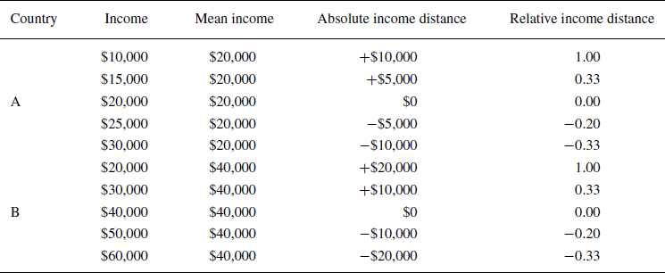
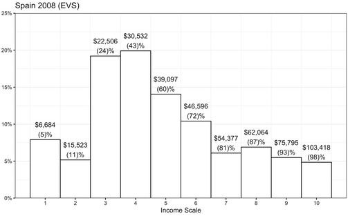
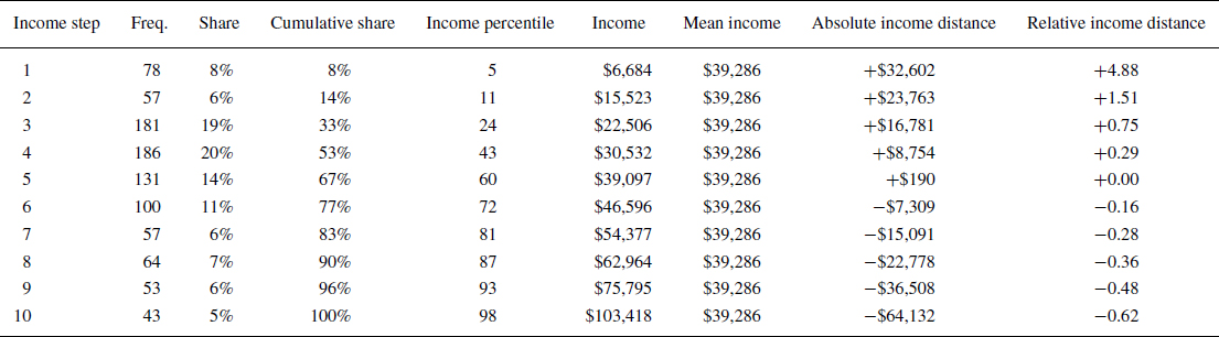
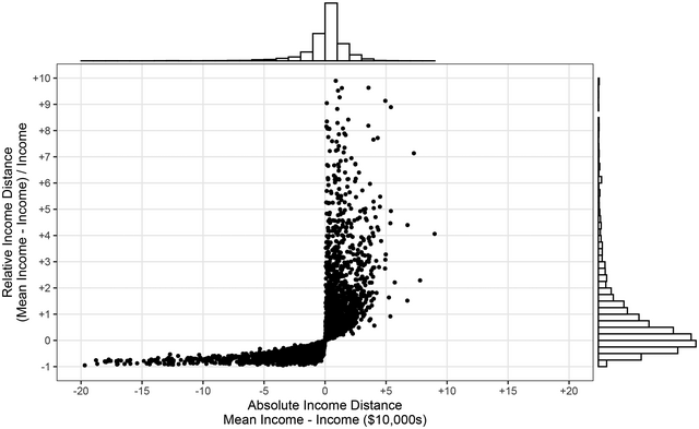
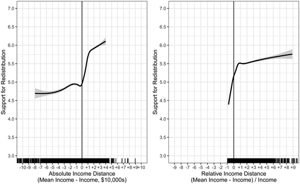

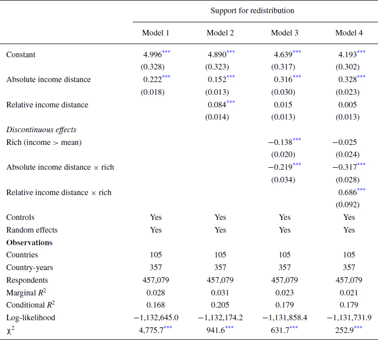
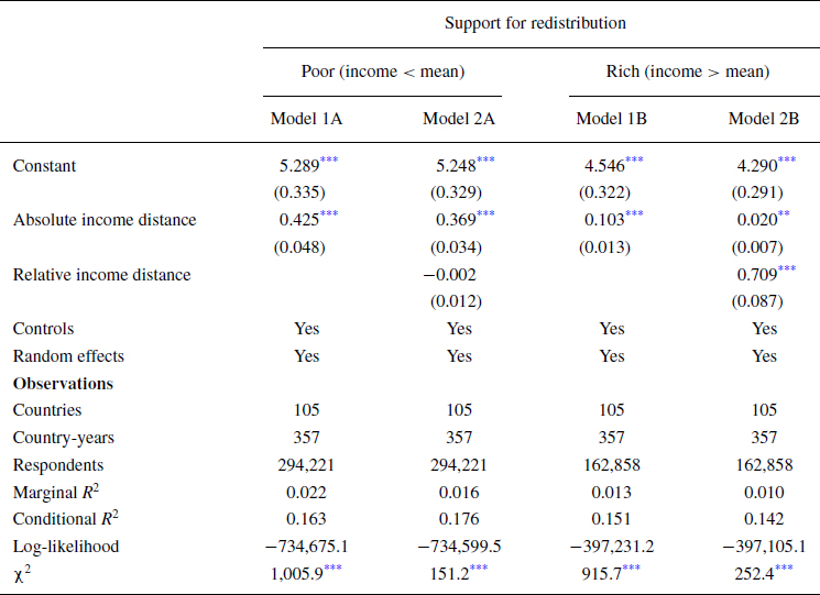
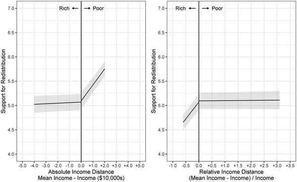
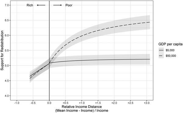
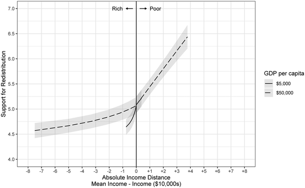
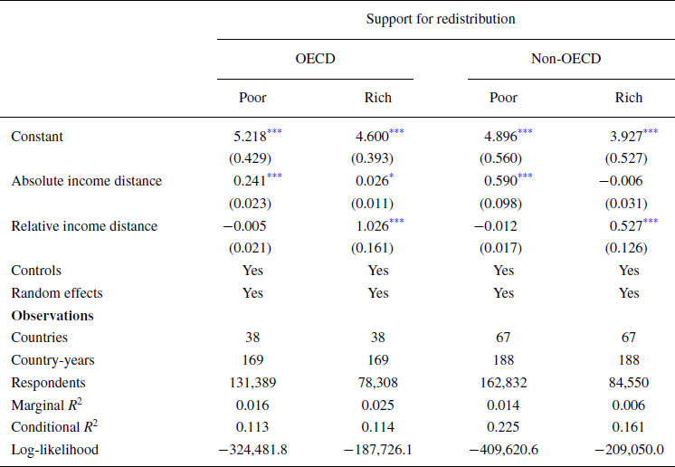


 Open access