


1. Introduction
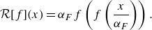
The Taylor–Couette flow, driven by two independently rotating coaxial cylinders (figure 1 a), has been a prominent research topic in fluid dynamics for over a century. By varying the angular velocities of the cylinders in experimental set-ups, a rich variety of flow patterns can be observed, as documented by Andereck, Liu & Swinney (Reference Andereck, Liu and Swinney1986). In this paper, we focus on the case with counter-rotating cylinders, a regime for which Taylor–Couette flow has long served as a paradigm of subcritical transition to turbulence. The onset of fully developed turbulence is preceded by intermittency, with the flow typically exhibiting alternating laminar and turbulent helical bands (Coles Reference Coles1965; Dong Reference Dong2009; Meseguer et al. Reference Meseguer, Mellibovsky, Avila and Marques2009b ); see figure 1(b).
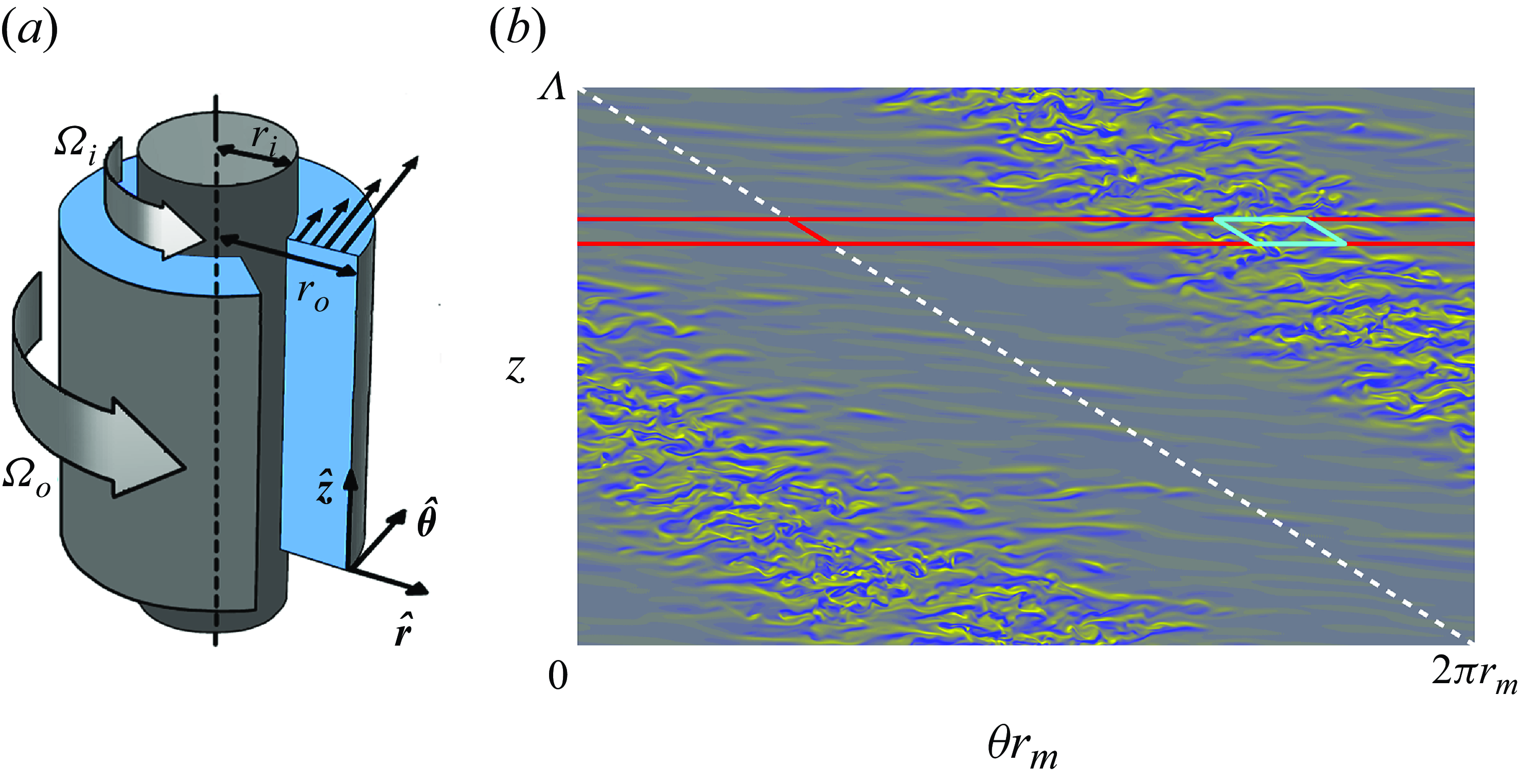
Figure 1. Taylor–Couette flow. (a) Sketch of the flow configuration. The inner and outer cylinders have radii $r=r_i$
and
$r=r_i$
and $r=r_o$
, respectively, and rotate with angular velocities
$r=r_o$
, respectively, and rotate with angular velocities $\Omega _i$
and
$\Omega _i$
and $\Omega _o$
. (b) A snapshot of the stripe pattern adopted from figure 2 of Wang et al. (Reference Wang, Ayats, Deguchi, Mellibovsky and Meseguer2022). The colour map shows the radial vorticity at the mid gap
$\Omega _o$
. (b) A snapshot of the stripe pattern adopted from figure 2 of Wang et al. (Reference Wang, Ayats, Deguchi, Mellibovsky and Meseguer2022). The colour map shows the radial vorticity at the mid gap $r_m=(r_o+r_i)/2$
. The radius ratio and inner and outer cylinder Reynolds numbers, defined in § 2, are set to
$r_m=(r_o+r_i)/2$
. The radius ratio and inner and outer cylinder Reynolds numbers, defined in § 2, are set to $(\eta ,R_i,R_o)=(0.883,600,-1200)$
.
$(\eta ,R_i,R_o)=(0.883,600,-1200)$
.
The mean flow topology of these helical bands (Wang et al. Reference Wang, Mellibovsky, Ayats, Deguchi and Meseguer2023) has recently been shown to resemble the laminar–turbulent stripe pattern observed in plane Couette flow (Barkley & Tuckerman Reference Barkley and Tuckerman2007). Indeed, large-scale intermittent patterns of coexisting turbulent and laminar regions are ubiquitous in wall-bounded subcritical shear flows (Tuckerman, Chantry & Barkley Reference Tuckerman, Chantry and Barkley2020). Stochastic approaches, such as directed percolation theory, are gaining popularity as a framework for understanding the onset of subcritical turbulent transition (Hof Reference Hof2023). However, applying stochastic arguments to a deterministic system inherently assumes the pre-existence of chaotic dynamics. In the case of subcritical shear flows, identifying the emergence of chaos that precedes turbulent transition poses a significant challenge.
What complicates the detailed understanding of transitional and fully developed turbulence in shear flows, with all the subtle features it encompasses, is the multi-scale nature of the flow. Consequently, many aspects of subcritical parallel shear flow turbulence have historically been approached using small periodic computational domains called minimal flow units (Jiménez & Moin Reference Jiménez and Moin1991; Hamilton, Kim & Waleffe Reference Hamilton, Kim and Waleffe1995; Kawahara, Uhlmann & van Veen Reference Kawahara, Uhlmann and van Veen2012). In Taylor–Couette flow, the use of minimal boxes has been common since the early stages of simulations (e.g. Marcus Reference Marcus1984; Coughlin & Marcus Reference Coughlin and Marcus1992). However, most studies employed parameters in the supercritical regime, and somewhat surprisingly, research in the subcritical regime remains rare. A recent review paper (Feldmann et al. Reference Feldmann, Borrero-Echeverry, Burin, Avila and Avila2023) hypothesised a connection between subcritical Taylor–Couette flow and plane Couette flow, for which Kreilos & Eckhardt (Reference Kreilos and Eckhardt2012) reported a period-doubling cascade leading to chaos in a small periodic box. Here, we confirm that a period-doubling route to chaos does indeed occur in Taylor–Couette flow within the parameter range studied by Meseguer et al. (Reference Meseguer, Mellibovsky, Avila and Marques2009b ), Deguchi, Meseguer & Mellibovsky (Reference Deguchi, Meseguer and Mellibovsky2014) and Wang et al. (Reference Wang, Ayats, Deguchi, Mellibovsky and Meseguer2022), the latter hereafter abbreviated as W22.
The most suitable flow unit for the parameter regime we address here is of annular-parallelogram shape proposed by Deguchi & Altmeyer (Reference Deguchi and Altmeyer2013). W22 first used a narrow elongated domain (red box in figure 1 b) to compute turbulent stripes in their minimal natural box, a strategy that has been repeatedly adopted in plane Couette (Barkley & Tuckerman Reference Barkley and Tuckerman2007) and channel flows (Tuckerman et al. Reference Tuckerman, Kreilos, Schrobsdorff, Schneider and Gibson2014). The domain was subsequently shortened in the azimuthal direction (cyan box in figure 1 b) so as to fit only one streamwise wavelength of a typical coherent structure of developed turbulence. As reported by W22, the use of such a domain was instrumental in observing the first few period-doubling bifurcations in the route to chaos. In this paper, we show that the ensuing period-doubling cascade aligns exceptionally well with Feigenbaum universality (Feigenbaum Reference Feigenbaum1978, Reference Feigenbaum1979, Reference Feigenbaum1980, Reference Feigenbaum1982).
1.1. Feigenbaum cascade in fluid flows
Feigenbaum universality became widely recognised among fluid dynamicists following the natural convection experiment conducted by Libchaber, Laroche & Fauve (Reference Libchaber, Laroche and Fauve1982), which led to the first empirical approximation of Feigenbaum’s first constant, $\delta _{{F}} \approx 4.6692016$
, corresponding to the limiting ratio of a period-doubling bifurcation interval to the next (see also the recent article by Libchaber (Reference Libchaber2023)). Their value,
$\delta _{{F}} \approx 4.6692016$
, corresponding to the limiting ratio of a period-doubling bifurcation interval to the next (see also the recent article by Libchaber (Reference Libchaber2023)). Their value, $\delta _4=4.4\pm 0.1$
, estimated from up to the fourth period-doubling bifurcation point (hence the subscript
$\delta _4=4.4\pm 0.1$
, estimated from up to the fourth period-doubling bifurcation point (hence the subscript $n=4$
), was not too distant from the theoretical value
$n=4$
), was not too distant from the theoretical value $\delta _{{F}}$
. Buzug, von Stamm & Pfister (Reference Buzug, von Stamm and Pfister1993) found an estimate close to
$\delta _{{F}}$
. Buzug, von Stamm & Pfister (Reference Buzug, von Stamm and Pfister1993) found an estimate close to $\delta _{{F}}$
when studying a Taylor–Couette apparatus with a tilted lid, while subsequent experimental efforts, summarised in table 1, resulted in persistently larger discrepancies. Estimates compatible with Feigenbaum’s first universal constant have also been obtained numerically for various fluid systems. Some of the values reported for
$\delta _{{F}}$
when studying a Taylor–Couette apparatus with a tilted lid, while subsequent experimental efforts, summarised in table 1, resulted in persistently larger discrepancies. Estimates compatible with Feigenbaum’s first universal constant have also been obtained numerically for various fluid systems. Some of the values reported for $\delta _n$
, also listed in table 1, are reasonably close to
$\delta _n$
, also listed in table 1, are reasonably close to $\delta _{{F}}$
at first glance. However, it must be borne in mind that the reliability of the approximations depends strongly on the number of consecutive period-doubling bifurcations analysed and is extremely sensitive to the accuracy with which they are located. Unfortunately, the approximate determinations of
$\delta _{{F}}$
at first glance. However, it must be borne in mind that the reliability of the approximations depends strongly on the number of consecutive period-doubling bifurcations analysed and is extremely sensitive to the accuracy with which they are located. Unfortunately, the approximate determinations of $\delta _{{F}}$
we have found in the literature of fluid flows were not accompanied with a detailed analysis as done, for example, for the Kuramoto–Sivashinsky equation (Smyrlis & Papageorgiou Reference Smyrlis and Papageorgiou1991). Accordingly, their reliability is debatable, as concluding Feigenbaum universality from a handful of period-doubled solutions is, at the very least, perilous.
$\delta _{{F}}$
we have found in the literature of fluid flows were not accompanied with a detailed analysis as done, for example, for the Kuramoto–Sivashinsky equation (Smyrlis & Papageorgiou Reference Smyrlis and Papageorgiou1991). Accordingly, their reliability is debatable, as concluding Feigenbaum universality from a handful of period-doubled solutions is, at the very least, perilous.
Table 1. Feigenbaum universality analyses in fluid systems. The table includes the number of period doubling bifurcations analysed ( $n$
), and the experimental (E) or numerical (N) nature of the study. An approximation to Feigenbaum’s first constant, estimated from the last three period-doubling bifurcations analysed in each case, is given in column
$n$
), and the experimental (E) or numerical (N) nature of the study. An approximation to Feigenbaum’s first constant, estimated from the last three period-doubling bifurcations analysed in each case, is given in column $\delta _n$
.
$\delta _n$
.

All the studies presented in table 1 explore period-doubling cascades that follow from a supercritical sequence of bifurcations of the base laminar flow. We focus instead on the subcritical regime, where turbulent transition may occur despite the linear stability of the base flow and can only be triggered by finite amplitude perturbations. The detection and study of period-doubling bifurcations emanating from unstable solutions is impracticable, and stable finite-amplitude solutions in the subcritical regime of shear flows that could potentially originate a cascade are rare and hard to find. The aforementioned study by Kreilos & Eckhardt (Reference Kreilos and Eckhardt2012) was the first to show that period-doubling cascades may also occur in subcritical transition problems. Their approach consisted in selecting the smallest possible periodic domain that is capable of sustaining turbulence in plane Couette flow while, at the same time, imposing specific discrete symmetries to further constrain the dynamics. Unfortunately, the resolution of their parametric exploration was insufficient to positively confirm universality. Symmetry restrictions were also employed by Moore et al. (Reference Moore, Toomre, Knobloch and Weiss1983) and Van Veen (Reference Van Veen2005) in their respective works. A similar period-doubling cascade in plane Couette flow has also been reported in a more recent paper by Lustro et al. (Reference Lustro, Kawahara, van Veen, Shimizu and Kokubu2019). However, calculation of $\delta _{{F}}$
in the subcritical regime of fluid flow problems has not been conducted to date.
$\delta _{{F}}$
in the subcritical regime of fluid flow problems has not been conducted to date.
1.2. Mathematical aspects of the Feigenbaum cascade
Although period-doubling cascades have been known to occur for over a century (Collet Reference Collet2019), universality was not discovered until much later by Feigenbaum (Reference Feigenbaum1978) and Coullet & Tresser (Reference Coullet and Tresser1978) independently, hence its being often referred to as Feigenbaum–Coullet–Tresser universality by mathematicians. The existence of universality swiftly spread throughout the mathematical community, as vividly depicted by Khanin et al. (Reference Khanin, Lyubich, Siggia and Sinai2021). Since its unveiling, universality has been repeatedly observed in numerical simulations of low-dimensional systems of ordinary differential equations. Checking universality in low-dimensional models like the Rössler system or the Duffing equation has become a common academic exercise. Feigenbaum universality was originally established within the framework of discrete dynamical systems based on one-dimensional iterated maps of the form $x_{\ell +1}=f(x_{\ell })$
,
$x_{\ell +1}=f(x_{\ell })$
, $\ell \in \mathbb {N}$
, with
$\ell \in \mathbb {N}$
, with $f(x)$
a unimodal function. Its necessary occurrence in continuous time dynamical systems is typically justified by the use of Poincaré sections. The phenomenon is often illustrated by initially replacing the Smale horseshoe that occurs on the Poincaré section with a Hénon map, which reduces to the logistic map in the limiting case of vanishing area contraction rate after one mapping. Then, since the logistic map is a unimodal map, universality of the period-doubling cascade can be explained by means of renormalisation theory, as done in many standard textbooks such as those by Collet & Eckmann (Reference Collet and Eckmann1980), Schuster (Reference Schuster1988), Glendinning (Reference Glendinning1994) or Strogatz (Reference Strogatz2024). Universality shows in both the parameter (coordinate) and state (ordinate) axes of the bifurcation diagram, the scaling in the latter axis is related to Feigenbaum’s second constant,
$f(x)$
a unimodal function. Its necessary occurrence in continuous time dynamical systems is typically justified by the use of Poincaré sections. The phenomenon is often illustrated by initially replacing the Smale horseshoe that occurs on the Poincaré section with a Hénon map, which reduces to the logistic map in the limiting case of vanishing area contraction rate after one mapping. Then, since the logistic map is a unimodal map, universality of the period-doubling cascade can be explained by means of renormalisation theory, as done in many standard textbooks such as those by Collet & Eckmann (Reference Collet and Eckmann1980), Schuster (Reference Schuster1988), Glendinning (Reference Glendinning1994) or Strogatz (Reference Strogatz2024). Universality shows in both the parameter (coordinate) and state (ordinate) axes of the bifurcation diagram, the scaling in the latter axis is related to Feigenbaum’s second constant, $\alpha _{{F}}\approx -2.5029079$
. In renormalisation theory,
$\alpha _{{F}}\approx -2.5029079$
. In renormalisation theory, $\alpha _{{F}}$
and the Feigenbaum function
$\alpha _{{F}}$
and the Feigenbaum function $G$
uniquely solve the Feigenbaum–Cvitanović functional equation
$G$
uniquely solve the Feigenbaum–Cvitanović functional equation $\mathcal {R}[G]=G$
(Feigenbaum Reference Feigenbaum1978; Cvitanović Reference Cvitanović1989), with the condition
$\mathcal {R}[G]=G$
(Feigenbaum Reference Feigenbaum1978; Cvitanović Reference Cvitanović1989), with the condition $G(0)=1$
. Here, the action of the renormalisation operator,
$G(0)=1$
. Here, the action of the renormalisation operator, $\mathcal {R}$
, on a function
$\mathcal {R}$
, on a function $f$
consists merely in the twice repeated application of
$f$
consists merely in the twice repeated application of $f$
, mediated by a rescaling that involves a factor
$f$
, mediated by a rescaling that involves a factor $\alpha _{{F}}$
:
$\alpha _{{F}}$
:
 \begin{eqnarray} \mathcal {R}[f](x)=\alpha _{{F}} f \left (f \left (\frac {x}{\alpha _{{F}}} \right )\right ). \end{eqnarray}
Despite its simplicity, this operator lies at the heart of the various instances of self-similarity that arise in the bifurcation diagram of the map generated by $f$
. Likewise, Feigenbaum’s first constant
$f$
. Likewise, Feigenbaum’s first constant $\delta _{{F}}$
is the leading eigenvalue of the linearisation around
$\delta _{{F}}$
is the leading eigenvalue of the linearisation around $G$
of the renormalisation operator
$G$
of the renormalisation operator $\mathcal {R}$
, and
$\mathcal {R}$
, and $\varPhi$
is the associated eigenfunction (Lanford III Reference Lanford III1982; Epstein Reference Epstein1986; Eckmann & Wittwer Reference Eckmann and Wittwer1987; Briggs Reference Briggs1991; Stephenson & Wang Reference Stephenson and Wang1991), which has recently been dubbed Feigenfunction by Thurlby (Reference Thurlby2021), as a tribute to Feigenbaum. The first mathematical proof of the existence of the universal constants,
$\varPhi$
is the associated eigenfunction (Lanford III Reference Lanford III1982; Epstein Reference Epstein1986; Eckmann & Wittwer Reference Eckmann and Wittwer1987; Briggs Reference Briggs1991; Stephenson & Wang Reference Stephenson and Wang1991), which has recently been dubbed Feigenfunction by Thurlby (Reference Thurlby2021), as a tribute to Feigenbaum. The first mathematical proof of the existence of the universal constants, $\delta _{{F}}$
and
$\delta _{{F}}$
and $\alpha _{{F}}$
, and functions,
$\alpha _{{F}}$
, and functions, $G$
and
$G$
and $\varPhi$
, is attributed to Lanford III (Reference Lanford III1982).
$\varPhi$
, is attributed to Lanford III (Reference Lanford III1982).
Ascertaining universality from the ability to reproduce $\delta _{{F}}$
and
$\delta _{{F}}$
and $\alpha _{{F}}$
in fluid flow problems presents a twofold challenge. First, a numerical analysis analogous to that of low-dimensional models demands significantly higher computational resources when dealing with the Navier–Stokes equations. The first observation of
$\alpha _{{F}}$
in fluid flow problems presents a twofold challenge. First, a numerical analysis analogous to that of low-dimensional models demands significantly higher computational resources when dealing with the Navier–Stokes equations. The first observation of $\delta _{{F}}$
in the field of computational fluid mechanics was contributed by Moore et al. (Reference Moore, Toomre, Knobloch and Weiss1983) when analysing two-dimensional thermosolutal convection. It took, however, until Van Veen (Reference Van Veen2005) to expose universality in a three-dimensional set-up, and even then, only for a fluid contained in the simplest computational domain, i.e. periodic in all three space directions. Second, identifying flow configurations that exhibit the specific route to chaos being targeted, among the several possible in multi-dimensional systems, is much more difficult in physically relevant problems than in engineered toy models with tunable parameters. Cascades sequentially doubling the period at every bifurcation may occur through mechanisms quite different from those leading to universality (e.g. Yanagida Reference Yanagida1987; Kokubu, Komuro & Oka Reference Kokubu, Komuro and Oka1996; Homburg, Kokubu & Naudot Reference Homburg, Kokubu and Naudot2001; Yalim, Welfert & Lopez Reference Yalim, Welfert and Lopez2019). Other routes to chaos are also common in fluid systems; in the Taylor–Couette system, for example, chaos has been found to arise following the Ruelle–Takens–Newhouse scenario (Swinney & Gollub Reference Swinney and Gollub1985) or Shil’nikov-type bifurcations (Lopez & Marques Reference Lopez and Marques2005). All these difficulties justify why demonstrating Feigenbaum universality in a fluid system requires careful analysis.
$\delta _{{F}}$
in the field of computational fluid mechanics was contributed by Moore et al. (Reference Moore, Toomre, Knobloch and Weiss1983) when analysing two-dimensional thermosolutal convection. It took, however, until Van Veen (Reference Van Veen2005) to expose universality in a three-dimensional set-up, and even then, only for a fluid contained in the simplest computational domain, i.e. periodic in all three space directions. Second, identifying flow configurations that exhibit the specific route to chaos being targeted, among the several possible in multi-dimensional systems, is much more difficult in physically relevant problems than in engineered toy models with tunable parameters. Cascades sequentially doubling the period at every bifurcation may occur through mechanisms quite different from those leading to universality (e.g. Yanagida Reference Yanagida1987; Kokubu, Komuro & Oka Reference Kokubu, Komuro and Oka1996; Homburg, Kokubu & Naudot Reference Homburg, Kokubu and Naudot2001; Yalim, Welfert & Lopez Reference Yalim, Welfert and Lopez2019). Other routes to chaos are also common in fluid systems; in the Taylor–Couette system, for example, chaos has been found to arise following the Ruelle–Takens–Newhouse scenario (Swinney & Gollub Reference Swinney and Gollub1985) or Shil’nikov-type bifurcations (Lopez & Marques Reference Lopez and Marques2005). All these difficulties justify why demonstrating Feigenbaum universality in a fluid system requires careful analysis.
1.3. Accumulation point of the cascade and beyond
The orbits of ever increasing period that arise in succession as the parameter is varied along the period-doubling cascade pile up at the accumulation point, beyond which chaotic dynamics ensues. Our interest extends also to phenomena occurring past this point. The existence of a reverse cascade, whereby chaotic bands successively merge in pairs as one moves away from the accumulation point, is a well-established property of simple model maps (Grossmann & Thomae Reference Grossmann and Thomae1977; Lorenz Reference Lorenz1980). It is noteworthy that Huberman & Rudnick (Reference Huberman and Rudnick1980) observed self-similarity in the numerical analysis of Lyapunov exponents at the onset of chaos. Nevertheless, the extent to which universality holds in the chaotic regime remains an elusive question. Libchaber (Reference Libchaber and Garrido1983) tried to detect universality beyond the accumulation point in a natural convection experiment. To the authors’ knowledge, this is the first and only endeavour to unveil universality past the accumulation point of a period-doubling cascade in a fluid dynamics problem, but the results were rather crude due to experimental limitations. In theory, if universality holds beyond the accumulation point, the bifurcation diagram should be predictable, not only up to but also past this point, from the initial few period-doubling bifurcations. However, we have not been able to find any such attempts in the literature, even for low-dimensional models. While self-similarity of the reverse cascade past the accumulation point has been invariably observed and has been conjectured to hold universally, the underlying mechanisms remain unknown.
1.4. Outline of the paper
The paper is structured as follows. The problem formulation is presented in § 2, alongside a brief account of the numerical methods employed. Section 3 introduces the period-doubling cascade that is our object of study and illustrates the procedure by which period-doubling bifurcation points are accurately computed. The sequence of the first few such points is then exploited in § 4 to assess agreement with the first and second Feigenbaum constants and to extrapolate the expected occurrence of the accumulation point. A method for the detailed prediction of the bifurcation diagram in the neighbourhood of the accumulation point from just a few initial period-doubling bifurcations is devised in § 5. We further show how meaningful predictions can be made, in a statistical sense, that extend beyond the accumulation point into the chaotic regime. Finally, the main findings are summarised and conclusions drawn in § 6.
2. Formulation of the problem
We consider an incompressible Newtonian fluid of kinematic viscosity $\nu$
, filling the gap between two infinitely long concentric rotating cylinders (figure 1
a). The angular velocities of the inner and outer cylinders, of radii
$\nu$
, filling the gap between two infinitely long concentric rotating cylinders (figure 1
a). The angular velocities of the inner and outer cylinders, of radii $r^*_{i}$
and
$r^*_{i}$
and $r^*_{o}$
, are denoted as
$r^*_{o}$
, are denoted as $\Omega _{i}$
and
$\Omega _{i}$
and $\Omega _{o}$
, respectively. A complete set of independent dimensionless physical parameters characterising the problem are the radius ratio
$\Omega _{o}$
, respectively. A complete set of independent dimensionless physical parameters characterising the problem are the radius ratio $\eta =r^*_{i}/r^*_{o}$
and the two Reynolds numbers
$\eta =r^*_{i}/r^*_{o}$
and the two Reynolds numbers $R_i={\textrm{d}}r^*_{i}\Omega _{i}/\nu$
and
$R_i={\textrm{d}}r^*_{i}\Omega _{i}/\nu$
and $R_o={\textrm{d}}r^*_{o}\Omega _{o}/\nu$
, where
$R_o={\textrm{d}}r^*_{o}\Omega _{o}/\nu$
, where $d=r^*_{o}-r^*_{i}$
is the gap.
$d=r^*_{o}-r^*_{i}$
is the gap.
All variables are rendered dimensionless using $d$
and
$d$
and $d^2/\nu$
as units for space and time, respectively. In cylindrical coordinates
$d^2/\nu$
as units for space and time, respectively. In cylindrical coordinates $(r,\theta ,z)$
, the velocity
$(r,\theta ,z)$
, the velocity $\boldsymbol {v}=(v_r,v_{\theta },v_z)=v_r\,\hat {\boldsymbol {r}} + v_{\theta }\,\hat {\boldsymbol { \theta }} + v_z\,\hat {\boldsymbol {z}}$
and pressure
$\boldsymbol {v}=(v_r,v_{\theta },v_z)=v_r\,\hat {\boldsymbol {r}} + v_{\theta }\,\hat {\boldsymbol { \theta }} + v_z\,\hat {\boldsymbol {z}}$
and pressure $p$
of the fluid are governed by the Navier–Stokes equations, the incompressibility condition and the zero axial net massflux condition, i.e.
$p$
of the fluid are governed by the Navier–Stokes equations, the incompressibility condition and the zero axial net massflux condition, i.e.
 \begin{align} &\partial _{t}\boldsymbol {v} + (\boldsymbol {v}\cdot \nabla )\boldsymbol {v} = -\nabla p + \nabla ^{2}\boldsymbol {v} + f\,\hat {\boldsymbol {z}}, \end{align}
 \begin{align} &\qquad\qquad\qquad \nabla \cdot \boldsymbol {v} = 0, \end{align}
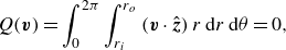 \begin{align} &Q(\boldsymbol {v}) = \int _0^{2\pi }{\int _{r_{i}}^{r_{o}}{(\boldsymbol {v}\cdot \hat {\boldsymbol {z}})\,r\,{\textrm{d}}r\,{\textrm{d}}\theta }} = 0, \\[6pt] \nonumber \end{align}
where the axial forcing term $f=f(t)$
in (2.1) is instantaneously adjusted to fulfil the constraint imposed by (2.3). The no-slip boundary conditions at the cylinder walls are
$f=f(t)$
in (2.1) is instantaneously adjusted to fulfil the constraint imposed by (2.3). The no-slip boundary conditions at the cylinder walls are
 \begin{equation} \boldsymbol {v}(r_i,\theta ,z)=(0,R_i,0),\quad \boldsymbol {v}(r_o,\theta ,z)=(0,R_o,0), \end{equation}
with $r_i=r_i^*/d=\eta /(1-\eta )$
and
$r_i=r_i^*/d=\eta /(1-\eta )$
and $r_o=r_o^*/d=1/(1-\eta )$
. The base, laminar and steady circular Couette flow, henceforth referred to as CCF, has
$r_o=r_o^*/d=1/(1-\eta )$
. The base, laminar and steady circular Couette flow, henceforth referred to as CCF, has
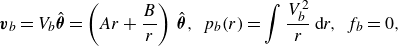 \begin{equation} \boldsymbol {v}_{{b}} = V_{{b}} \hat {\boldsymbol {\theta }} = \displaystyle \left (Ar+\frac {B}{r}\right )\,\hat {\boldsymbol {\theta }}, \;\; p_{{b}}(r)=\int \frac {V_{{b}}^2}{r} \,\textrm {d}r, \;\; f_{{b}} = 0, \end{equation}
with $ A=(R_o-\eta R_i)/(1+\eta )$
and
$ A=(R_o-\eta R_i)/(1+\eta )$
and $B=\eta (R_i-\eta R_o)/ [(1-\eta )(1-\eta ^2) ]$
. In what follows, we express the velocity and pressure fields as
$B=\eta (R_i-\eta R_o)/ [(1-\eta )(1-\eta ^2) ]$
. In what follows, we express the velocity and pressure fields as
 \begin{equation} \boldsymbol {v} = \boldsymbol {v}_{{b}}(r) + \mathbf {u}(r,\theta ,z;t), \quad p=p_{{b}}(r) + q(r,\theta ,z;t). \end{equation}
The fields $q$
and
$q$
and $\mathbf {u}= u_r\,\hat {\boldsymbol {r}} + u_{\theta }\,\hat {\boldsymbol {\theta }} + u_z\,\hat {\boldsymbol {z}}$
are the deviations from the CCF solution. The nonlinear boundary value problem for
$\mathbf {u}= u_r\,\hat {\boldsymbol {r}} + u_{\theta }\,\hat {\boldsymbol {\theta }} + u_z\,\hat {\boldsymbol {z}}$
are the deviations from the CCF solution. The nonlinear boundary value problem for $\mathbf {u}$
and
$\mathbf {u}$
and $q$
is discretised using a solenoidal Petrov–Galerkin spectral scheme described by Meseguer et al. (Reference Meseguer, Avila, Mellibovsky and Marques2007). The unknown perturbation fields are approximated by means of a Chebyshev
$q$
is discretised using a solenoidal Petrov–Galerkin spectral scheme described by Meseguer et al. (Reference Meseguer, Avila, Mellibovsky and Marques2007). The unknown perturbation fields are approximated by means of a Chebyshev $\times$
Fourier
$\times$
Fourier $\times$
Fourier spectral expansion in
$\times$
Fourier spectral expansion in $(r,\theta ,z)$
, but in the annular-parallelogram domain
$(r,\theta ,z)$
, but in the annular-parallelogram domain $(r,\xi ,\zeta ) \in [r_{i},r_{o} ]\times [ 0,2\pi ] \times [ 0,2\pi ]$
, where the
$(r,\xi ,\zeta ) \in [r_{i},r_{o} ]\times [ 0,2\pi ] \times [ 0,2\pi ]$
, where the $2\pi$
-periodicity is imposed in the transformed coordinates
$2\pi$
-periodicity is imposed in the transformed coordinates
 \begin{equation} \xi = n_1\theta + k_1 z,\quad \zeta = n_2\theta + k_2 z, \end{equation}
following Deguchi & Altmeyer (Reference Deguchi and Altmeyer2013). Figure 2(a) shows the computational domain corresponding to $\eta =0.883$
and the wavenumber set
$\eta =0.883$
and the wavenumber set $(n_1,k_1,n_2,k_2)=(10,2,0,4.5)$
. The domain was specifically designed for the earliest onset of non-trivial solutions while keeping compatibility with the large-scale tilt of spiral turbulence. For this reason, the bifurcation scenario we investigate is fully compatible with the overall structure of intermittent patterns experimentally observed in the counter-rotating regime of the Taylor–Couette system and, at the same time, can be reasonably expected to precede any other mechanism potentially leading to the onset of chaos. All computations have been run in this domain. The same resolution of
$(n_1,k_1,n_2,k_2)=(10,2,0,4.5)$
. The domain was specifically designed for the earliest onset of non-trivial solutions while keeping compatibility with the large-scale tilt of spiral turbulence. For this reason, the bifurcation scenario we investigate is fully compatible with the overall structure of intermittent patterns experimentally observed in the counter-rotating regime of the Taylor–Couette system and, at the same time, can be reasonably expected to precede any other mechanism potentially leading to the onset of chaos. All computations have been run in this domain. The same resolution of $[0,50]\times [-8,8]\times [-8,8]$
modes as used in W22 has been employed throughout. The system of ordinary differential equations that results from spatial discretisation has dimension
$[0,50]\times [-8,8]\times [-8,8]$
modes as used in W22 has been employed throughout. The system of ordinary differential equations that results from spatial discretisation has dimension $O(10^5)$
.
$O(10^5)$
.
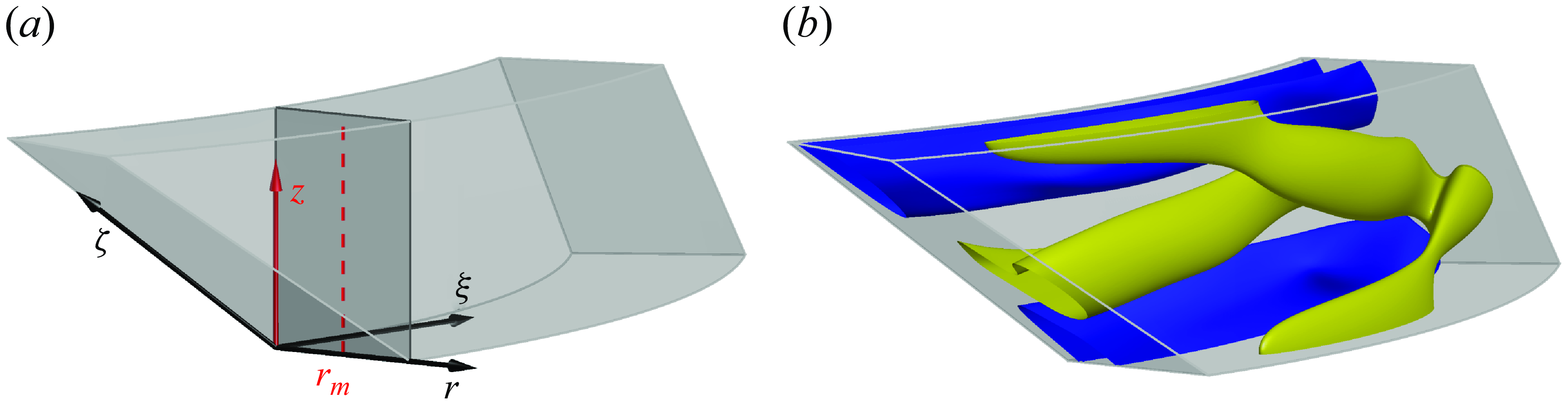
Figure 2. (a) Annular-parallelogram computational domain defined by the coordinates of (2.7) with wavenumbers $(n_1,k_1,n_2,k_2)=(10,2,0,4.5)$
and
$(n_1,k_1,n_2,k_2)=(10,2,0,4.5)$
and $\eta =0.883$
, adopted from W22. The axial line probe (red dashed vertical line) used in the production of space–time diagrams is located at mid gap
$\eta =0.883$
, adopted from W22. The axial line probe (red dashed vertical line) used in the production of space–time diagrams is located at mid gap $r_m=(r_i+r_o)/2 \approx 8.047$
. (b) Three-dimensional flow structure of DRW solution for
$r_m=(r_i+r_o)/2 \approx 8.047$
. (b) Three-dimensional flow structure of DRW solution for $(R_i,R_o) = (450,-1200)$
. Positive (yellow,
$(R_i,R_o) = (450,-1200)$
. Positive (yellow, $u_{\theta } = 250$
) and negative (blue,
$u_{\theta } = 250$
) and negative (blue, $u_{\theta } = -100$
) isosurfaces of perturbation azimuthal velocity.
$u_{\theta } = -100$
) isosurfaces of perturbation azimuthal velocity.
To explore the dynamically relevant invariant sets, we combine direct numerical simulation (DNS) with a Poincaré–Newton–Krylov (PNK) iterative scheme. The spectrally discretised Navier–Stokes equations are integrated in time using a fourth-order linearly implicit IMEX scheme. The PNK scheme, built on top of the time integrator, looks for zeroes of a map defined with a purposely devised Poincaré section by means of a Krylov-space-based Newton solver. For a detailed account of the numerical methods used, refer to Ayats et al. (Reference Ayats, Deguchi, Mellibovsky and Meseguer2020) and W22.
We characterise flow states by the normalised kinetic energy $\kappa$
of the perturbation velocity field, and by the corresponding inner and outer cylinders normalised torque,
$\kappa$
of the perturbation velocity field, and by the corresponding inner and outer cylinders normalised torque, $\tau _{i}$
and
$\tau _{i}$
and $\tau _{o}$
,
$\tau _{o}$
,
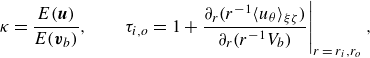 \begin{eqnarray} \kappa = \frac {E(\boldsymbol {u})}{E(\boldsymbol {v}_b)},\qquad \tau _{{i}, {o}}= \left . 1+\frac {\partial _r(r^{-1}\langle u_{\theta }\rangle _{\xi \zeta })}{\partial _r(r^{-1}V_{b})}\right |_{r\,=\,r_{i},r_{o}}, \end{eqnarray}
where
 \begin{equation} E(\boldsymbol {v}) = \frac {1}{2\mathcal {V}} \iiint _{\mathcal {V}}{\boldsymbol {v}\cdot \boldsymbol {v}\,{\textrm{d}}\mathcal {V}} = \frac {1}{2\mathcal {V}}\int _{0}^{2\pi }\!\int _{0}^{2\pi }\!\int _{r_{i}}^{r_{o}} \boldsymbol {v}\cdot \boldsymbol {v}\,r\,\textrm{d}r\textrm {d}\xi \textrm {d}\zeta = \frac {1-\eta }{1+\eta }\int _{r_{i}}^{r_{o}}{\langle \boldsymbol {v}\cdot \boldsymbol {v}\rangle _{\xi \zeta }\,r\,\textrm {d}r} \end{equation}
is the volume-averaged kinetic energy of some velocity field $\boldsymbol {v}$
. The volume of the transformed computational domain is
$\boldsymbol {v}$
. The volume of the transformed computational domain is $\mathcal {V}=2\pi ^2(r_{o}^2-r_{i}^2)=2\pi ^2(1-\eta )/(1+\eta )$
and
$\mathcal {V}=2\pi ^2(r_{o}^2-r_{i}^2)=2\pi ^2(1-\eta )/(1+\eta )$
and $\langle \ \rangle _{\xi \zeta }$
implies averaging in both parallelogram directions. With these definitions,
$\langle \ \rangle _{\xi \zeta }$
implies averaging in both parallelogram directions. With these definitions, $\kappa =0$
and
$\kappa =0$
and $\tau _{i}=\tau _{o}=1$
for CCF.
$\tau _{i}=\tau _{o}=1$
for CCF.
The system possesses translational invariance in $\xi$
and
$\xi$
and $\zeta$
. We define the entire set of possible spectral coefficients as the phase space. All coefficient vectors that belong to the group orbit induced by translation of a velocity field represent the same solution. We have systematically factored out the group orbit invariance employing the method of slices (Budanur et al. Reference Budanur, Cvitanović, Davidchack and Siminos2015), using the same template as Wang et al. (Reference Wang, Mellibovsky, Ayats, Deguchi and Meseguer2023). To analyse the period-doubling cascade within the framework of discrete-time dynamical systems, we have devised a Poincaré section
$\zeta$
. We define the entire set of possible spectral coefficients as the phase space. All coefficient vectors that belong to the group orbit induced by translation of a velocity field represent the same solution. We have systematically factored out the group orbit invariance employing the method of slices (Budanur et al. Reference Budanur, Cvitanović, Davidchack and Siminos2015), using the same template as Wang et al. (Reference Wang, Mellibovsky, Ayats, Deguchi and Meseguer2023). To analyse the period-doubling cascade within the framework of discrete-time dynamical systems, we have devised a Poincaré section
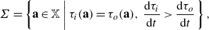 \begin{equation} \Sigma =\left \{{\mathbf{a}}\in \mathbb {X}\left |\;\tau _i({\mathbf{a}})=\tau _o({\mathbf{a}}),\;\dfrac {{\textrm{d}}\tau _i}{{\textrm{d}}t}\gt \dfrac {{\textrm{d}}\tau _o}{{\textrm{d}}t}\right . \right \}, \end{equation}
in phase space $\mathbb {X}$
, which consists of all possible sliced spectral expansion coefficients vector
$\mathbb {X}$
, which consists of all possible sliced spectral expansion coefficients vector $\mathbf {a}$
. The condition defining
$\mathbf {a}$
. The condition defining $\Sigma$
is based on the equality of inner and outer cylinder torque (first condition), and the sign of the rate of change of their difference (second condition) to discard reverse crossings. It is easy to check from the governing equations that for statistically steady states, the time average of
$\Sigma$
is based on the equality of inner and outer cylinder torque (first condition), and the sign of the rate of change of their difference (second condition) to discard reverse crossings. It is easy to check from the governing equations that for statistically steady states, the time average of $\tau _{i}$
must coincide with that of
$\tau _{i}$
must coincide with that of $\tau _{o}$
. Consequently, long-lived (including permanent) time-dependent solutions are bound to regularly fulfil the condition
$\tau _{o}$
. Consequently, long-lived (including permanent) time-dependent solutions are bound to regularly fulfil the condition $\tau _{i}=\tau _{o}$
, a property that comes in handy in defining a robust Poincaré section. To simplify notation, we will hereafter call
$\tau _{i}=\tau _{o}$
, a property that comes in handy in defining a robust Poincaré section. To simplify notation, we will hereafter call $\tau =\tau _i=\tau _o$
the value of the torque, whether inner or outer, on
$\tau =\tau _i=\tau _o$
the value of the torque, whether inner or outer, on $\Sigma$
.
$\Sigma$
.
There are other ways of sampling a continuous system to produce a discrete system. For example. Kreilos & Eckhardt (Reference Kreilos and Eckhardt2012) and Gao et al. (Reference Gao, Podvin, Sergent and Xin2015) investigated the relationship between consecutive local maxima of the time series of some physical quantity. However, it is not easy to discern which minima/maxima are actually related to the underlying (pseudo-)periodicity of the solutions and which are simply incidental to the dynamics of the particular time signal used. Thus, the use of the above tailor-made Poincaré section provides a more reliable approach.
3. Period-doubling cascade
Emulating the influential experiments by Andereck et al. (Reference Andereck, Liu and Swinney1986), we employ a radius ratio $\eta =0.883$
(
$\eta =0.883$
( $r \in [r_i,r_o]=[7.547,8.547]$
). The outer cylinder Reynolds number is fixed at
$r \in [r_i,r_o]=[7.547,8.547]$
). The outer cylinder Reynolds number is fixed at $R_o = -1200$
. For sufficiently large
$R_o = -1200$
. For sufficiently large $R_i$
, the centrifugal instability of the base flow develops into fully fledged turbulence. A reduction of
$R_i$
, the centrifugal instability of the base flow develops into fully fledged turbulence. A reduction of $R_i$
, while still in the supercritical region, has the flow re-organise into a pattern of alternating laminar and turbulent winding helical bands, commonly known as the spiral turbulence regime (Coles Reference Coles1965; Andereck et al. Reference Andereck, Liu and Swinney1986; Dong Reference Dong2009; Meseguer et al. Reference Meseguer, Mellibovsky, Avila and Marques2009b
). At this particular value of
$R_i$
, while still in the supercritical region, has the flow re-organise into a pattern of alternating laminar and turbulent winding helical bands, commonly known as the spiral turbulence regime (Coles Reference Coles1965; Andereck et al. Reference Andereck, Liu and Swinney1986; Dong Reference Dong2009; Meseguer et al. Reference Meseguer, Mellibovsky, Avila and Marques2009b
). At this particular value of $R_o$
, the CCF is linearly stable for
$R_o$
, the CCF is linearly stable for $R_i \lesssim 447.35$
, but a number of subcritical nonlinear equilibrium states persist below this threshold (Meseguer et al. Reference Meseguer, Mellibovsky, Avila and Marques2009a
; Deguchi et al. Reference Deguchi, Meseguer and Mellibovsky2014; and W22), which are believed to act as precursors of spiral turbulence. Drawing from the helix angle of the turbulent stripes observed experimentally, W22 employed the domain and coordinate system shown in figure 2(a) to seek minimal flow unit solutions that are compatible with the tilt of the banded pattern. Subharmonic instabilities of some such solutions were proposed as the mechanism that might be responsible for the spatial intermittency characterising spiral turbulence. Within this minimal parallelogram-annular periodic domain, which is capable of sustaining turbulence at sufficiently high
$R_i \lesssim 447.35$
, but a number of subcritical nonlinear equilibrium states persist below this threshold (Meseguer et al. Reference Meseguer, Mellibovsky, Avila and Marques2009a
; Deguchi et al. Reference Deguchi, Meseguer and Mellibovsky2014; and W22), which are believed to act as precursors of spiral turbulence. Drawing from the helix angle of the turbulent stripes observed experimentally, W22 employed the domain and coordinate system shown in figure 2(a) to seek minimal flow unit solutions that are compatible with the tilt of the banded pattern. Subharmonic instabilities of some such solutions were proposed as the mechanism that might be responsible for the spatial intermittency characterising spiral turbulence. Within this minimal parallelogram-annular periodic domain, which is capable of sustaining turbulence at sufficiently high $R_i$
, W22 identified a stable finite amplitude travelling wave (shown in figure 2
b) that coexists with the stable CCF. This drifting rotating wave, DRW for short, embodies all the essential elements of the self-sustaining mechanism (Wang, Gibson & Waleffe Reference Wang, Gibson and Waleffe2007; Hall & Sherwin Reference Hall and Sherwin2010) and plays a central role in the transition process. In W22, two periodic solutions, P
$R_i$
, W22 identified a stable finite amplitude travelling wave (shown in figure 2
b) that coexists with the stable CCF. This drifting rotating wave, DRW for short, embodies all the essential elements of the self-sustaining mechanism (Wang, Gibson & Waleffe Reference Wang, Gibson and Waleffe2007; Hall & Sherwin Reference Hall and Sherwin2010) and plays a central role in the transition process. In W22, two periodic solutions, P $_1$
, arising from a Hopf bifurcation of DRW, and P
$_1$
, arising from a Hopf bifurcation of DRW, and P $_2$
, originating at a period-doubling bifurcation of P
$_2$
, originating at a period-doubling bifurcation of P $_1$
, were also identified as the first steps in the route to chaos. This sequence of bifurcations suggested a period-doubling cascade as the most plausible scenario for the onset of chaotic dynamics, but the issue was not pursued further.
$_1$
, were also identified as the first steps in the route to chaos. This sequence of bifurcations suggested a period-doubling cascade as the most plausible scenario for the onset of chaotic dynamics, but the issue was not pursued further.
3.1. Onset of the period-doubling cascade
We now look into the bifurcation sequence the system undergoes in the range $R_i\in [395.43,395.79]$
eventually leading to sustained chaotic dynamics. Since we will only be varying
$R_i\in [395.43,395.79]$
eventually leading to sustained chaotic dynamics. Since we will only be varying $R_i$
, we shall drop the subscript and simply write
$R_i$
, we shall drop the subscript and simply write $R$
to ease notation.
$R$
to ease notation.
Figure 3(a) shows the DRW (square), P $_1$
(dashed blue line) and P
$_1$
(dashed blue line) and P $_2$
(solid green line) at
$_2$
(solid green line) at $R=395.67$
in a three-dimensional projection of the full phase space
$R=395.67$
in a three-dimensional projection of the full phase space $\mathbb {X}$
on the subspace spanned by the triplet of key quantities
$\mathbb {X}$
on the subspace spanned by the triplet of key quantities $(\tau _o,\tau _i,\kappa )$
. The Poincaré section
$(\tau _o,\tau _i,\kappa )$
. The Poincaré section $\Sigma$
appears in this representation as the transparent grey plane, which contains DRW and is pierced, in the direction defined by (2.10), at a single point by P
$\Sigma$
appears in this representation as the transparent grey plane, which contains DRW and is pierced, in the direction defined by (2.10), at a single point by P $_1$
and at two different points by P
$_1$
and at two different points by P $_2$
. In the torque time series of figure 3(b), the Poincaré crossings are conveniently identified as the intersections between the
$_2$
. In the torque time series of figure 3(b), the Poincaré crossings are conveniently identified as the intersections between the $\tau _i$
(thick lines) and
$\tau _i$
(thick lines) and $\tau _o$
(thin) signals for which the former is overtaking the latter. The two-dimensional projection of figure 3(a) onto the plane
$\tau _o$
(thin) signals for which the former is overtaking the latter. The two-dimensional projection of figure 3(a) onto the plane $(\tau _o,\tau _i)$
, as depicted in figure 3(c), further clarifies how the sequence of intersection points of figure 3(b) collapses in phase space onto a single point for P
$(\tau _o,\tau _i)$
, as depicted in figure 3(c), further clarifies how the sequence of intersection points of figure 3(b) collapses in phase space onto a single point for P $_1$
(empty blue disk) and as two distinct points for P
$_1$
(empty blue disk) and as two distinct points for P $_2$
(filled green circles), all contained in
$_2$
(filled green circles), all contained in $\Sigma$
(dashed grey straight line).
$\Sigma$
(dashed grey straight line).

Figure 3. Poincaré section $\Sigma$
and the periodic orbits P
$\Sigma$
and the periodic orbits P $_1$
(dashed blue) and P
$_1$
(dashed blue) and P $_2$
(solid green). The black squares are DRW solutions. All solutions are computed at
$_2$
(solid green). The black squares are DRW solutions. All solutions are computed at $R=395.67$
. (a) Projection of the phase space on the
$R=395.67$
. (a) Projection of the phase space on the $(\tau _o,\tau _i,\kappa )$
coordinates. (b) Inner (
$(\tau _o,\tau _i,\kappa )$
coordinates. (b) Inner ( $\tau _i$
, thick lines) and outer (
$\tau _i$
, thick lines) and outer ( $\tau _o$
, thin) torque time series of P
$\tau _o$
, thin) torque time series of P $_1$
and P
$_1$
and P $_2$
. (c) Two-dimensional phase map projection on the
$_2$
. (c) Two-dimensional phase map projection on the $(\tau _o,\tau _i)$
plane. The Poincaré section is shown in transparent grey in panel (a) and as a dashed grey line in panel (c). The circles on the P
$(\tau _o,\tau _i)$
plane. The Poincaré section is shown in transparent grey in panel (a) and as a dashed grey line in panel (c). The circles on the P $_1$
(empty blue) and P
$_1$
(empty blue) and P $_2$
(filled green) curves correspond to their representation on
$_2$
(filled green) curves correspond to their representation on $\Sigma$
.
$\Sigma$
.
The drift dynamics of non-axisymmetric solutions in Taylor–Couette as we have here is inevitably masked when monitoring aggregate quantities such as torque or kinetic energy due to their spatial averaging properties. Point measurements are instead subject to drift-induced time dependence. Figure 4(ai) presents a space–time diagram of the axial vorticity distribution measured along a line probe that is fixed in the lab reference frame (red dashed line in figure 2
a). DRW, a relative equilibrium, is characterised by a solid-body motion composing axial translation and azimuthal rotation with constant phase velocities. As a result, the space–time diagram exhibits the repetition of a periodic pattern. The same line probe produces a quasi-periodic space–time diagram for P $_1$
, as shown in figure 4(bi).Here, P
$_1$
, as shown in figure 4(bi).Here, P $_1$
is a relative periodic orbit and, therefore, requires suitable shifts in both the
$_1$
is a relative periodic orbit and, therefore, requires suitable shifts in both the $z$
and
$z$
and $\theta$
directions to align the flow fields after every one period to reveal the space–time invariance. The effects of the drift can be suppressed by attaching the line probe to a moving reference frame defined with the method of slices (Budanur et al. Reference Budanur, Cvitanović, Davidchack and Siminos2015; Wang et al. Reference Wang, Mellibovsky, Ayats, Deguchi and Meseguer2023). In this reference frame, the space–time diagrams of DRW and P
$\theta$
directions to align the flow fields after every one period to reveal the space–time invariance. The effects of the drift can be suppressed by attaching the line probe to a moving reference frame defined with the method of slices (Budanur et al. Reference Budanur, Cvitanović, Davidchack and Siminos2015; Wang et al. Reference Wang, Mellibovsky, Ayats, Deguchi and Meseguer2023). In this reference frame, the space–time diagrams of DRW and P $_1$
(figures 4
aii and 4
bii) are greatly simplified, the former appearing as time-independent and the latter as purely time-periodic.
$_1$
(figures 4
aii and 4
bii) are greatly simplified, the former appearing as time-independent and the latter as purely time-periodic.
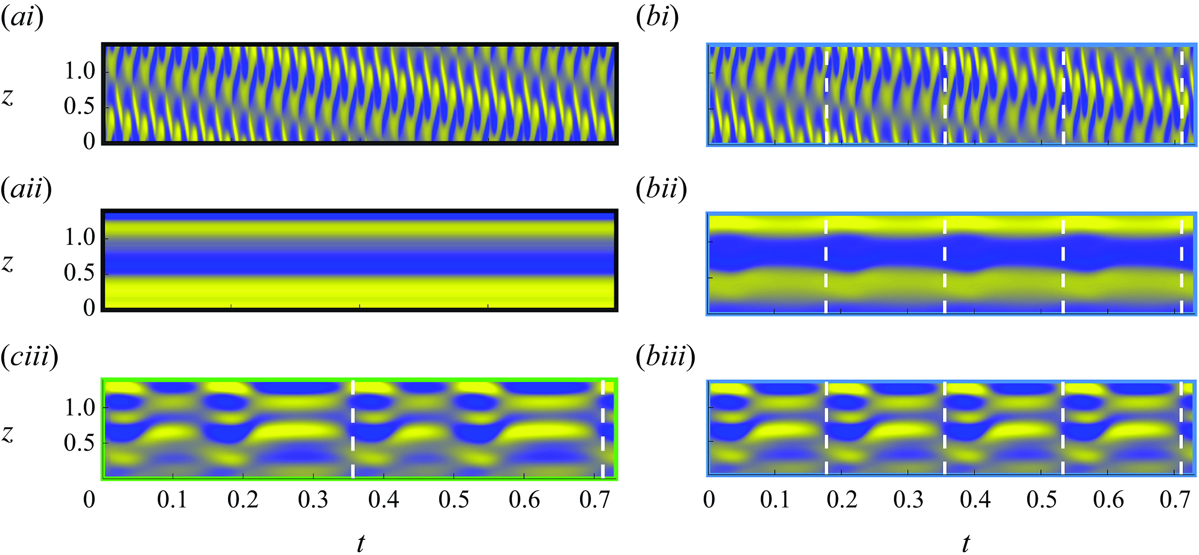
Figure 4. Space–time diagrams for (a) DRW, (b) P $_1$
and (c) P
$_1$
and (c) P $_2$
, all computed at
$_2$
, all computed at $R=395.67$
. The roman number labels denote measurements of radial vorticity
$R=395.67$
. The roman number labels denote measurements of radial vorticity $\omega _r(z;t)$
along axial probe lines at
$\omega _r(z;t)$
along axial probe lines at $(r,\theta )=(r_m,\theta _0)$
fixed to (i) the lab (stationary) reference frame, (ii) a reference frame co-moving with the solution and (iii) the same co-moving frame but with the temporal mean
$(r,\theta )=(r_m,\theta _0)$
fixed to (i) the lab (stationary) reference frame, (ii) a reference frame co-moving with the solution and (iii) the same co-moving frame but with the temporal mean $\langle \omega _r\rangle _{t}$
subtracted. The azimuthal location,
$\langle \omega _r\rangle _{t}$
subtracted. The azimuthal location, $\theta _0$
, is chosen consistently across reference frames and solutions to enable comparison. Colour shading according to
$\theta _0$
, is chosen consistently across reference frames and solutions to enable comparison. Colour shading according to $\omega _r\in [-1400,1400]$
or
$\omega _r\in [-1400,1400]$
or $\omega _r- \langle \omega _r\rangle _{t}\in [-300,300]$
, as need be. Dashed vertical lines indicate the natural period of the corresponding solution.
$\omega _r- \langle \omega _r\rangle _{t}\in [-300,300]$
, as need be. Dashed vertical lines indicate the natural period of the corresponding solution.
Further subtraction of the time average helps expose the true nature of the time dependence of the solutions. For P $_1$
, the time-horizon considered in figure 4(biii) allows for just over four repetitions, as indicated by the dashed vertical lines. Solution P
$_1$
, the time-horizon considered in figure 4(biii) allows for just over four repetitions, as indicated by the dashed vertical lines. Solution P $_2$
, shown in figure 4(ciii), has instead a natural period about twice that of P
$_2$
, shown in figure 4(ciii), has instead a natural period about twice that of P $_1$
, the period-doubling consisting in a modulation that shortens one of the half-periods while lengthening the other.
$_1$
, the period-doubling consisting in a modulation that shortens one of the half-periods while lengthening the other.
Let us now shift our focus to the dependence of the solutions on the parameter $R$
. Figure 5(a) shows the bifurcation sequence that DRW undergoes when varying the inner Reynolds number in the range
$R$
. Figure 5(a) shows the bifurcation sequence that DRW undergoes when varying the inner Reynolds number in the range $R\in [391.20,395.90]$
. DRW emerges from a saddle-node bifurcation (SN
$R\in [391.20,395.90]$
. DRW emerges from a saddle-node bifurcation (SN $_1$
) at
$_1$
) at $R\simeq 391.50$
and, leaving aside subharmonic instabilities, the nodal (upper) branch (the one represented in figure 2
b and the square in figure 3
a, 3
c) remains stable to perturbations fitting the domain until the advent of a supercritical Hopf bifurcation (H) at
$R\simeq 391.50$
and, leaving aside subharmonic instabilities, the nodal (upper) branch (the one represented in figure 2
b and the square in figure 3
a, 3
c) remains stable to perturbations fitting the domain until the advent of a supercritical Hopf bifurcation (H) at $R\simeq 392.85$
. As reported by W22, this is the only known case of a stable non-trivial solution in the subcritical parameter regime of Taylor–Couette flow. Note that, here, we are only interested in the stability to perturbations that fit within the periodic box. Stable/unstable solutions are denoted by solid/dashed lines. The PNK method must be used to compute unstable solution branches. A stable relative periodic orbit (P
$R\simeq 392.85$
. As reported by W22, this is the only known case of a stable non-trivial solution in the subcritical parameter regime of Taylor–Couette flow. Note that, here, we are only interested in the stability to perturbations that fit within the periodic box. Stable/unstable solutions are denoted by solid/dashed lines. The PNK method must be used to compute unstable solution branches. A stable relative periodic orbit (P $_1$
, blue line) bifurcates from DRW at H. All time-dependent solutions will be represented, from now on, through the collection of intersection points on the Poincaré section. The P
$_1$
, blue line) bifurcates from DRW at H. All time-dependent solutions will be represented, from now on, through the collection of intersection points on the Poincaré section. The P $_1$
branch becomes unstable in a period-doubling bifurcation (PD
$_1$
branch becomes unstable in a period-doubling bifurcation (PD $_1$
), whence a branch of stable period-doubled relative periodic orbits (P
$_1$
), whence a branch of stable period-doubled relative periodic orbits (P $_2$
, pair of green lines) emerges. The P
$_2$
, pair of green lines) emerges. The P $_2$
loses stability, in turn, in a second period-doubling bifurcation (PD
$_2$
loses stability, in turn, in a second period-doubling bifurcation (PD $_2$
) issuing a branch of period-4 solutions. The
$_2$
) issuing a branch of period-4 solutions. The $R$
value for which figures 3 and 4 were computed corresponds to just short of PD
$R$
value for which figures 3 and 4 were computed corresponds to just short of PD $_2$
, hence the instability of DRW and P
$_2$
, hence the instability of DRW and P $_1$
, in contrast with P
$_1$
, in contrast with P $_2$
, which is stable.
$_2$
, which is stable.

Figure 5. Bifurcation scenario as recorded on the Poincaré section $\Sigma$
. (a) Initial steps of the bifurcation scenario. Shown are DRW (black), P
$\Sigma$
. (a) Initial steps of the bifurcation scenario. Shown are DRW (black), P $_1$
(blue) and P
$_1$
(blue) and P $_2$
(green), reported in W22. P
$_2$
(green), reported in W22. P $_4$
(green) emerges at the second period-doubling bifurcation point PD
$_4$
(green) emerges at the second period-doubling bifurcation point PD $_2$
. Both stable (solid line) and unstable (dashed) solution branches are shown. (b) Detailed view (close-up of the region bounded by a solid grey box in panel a) of stable solution branches across the period-doubling cascade and beyond. The accumulation point for the period-doubling cascade (
$_2$
. Both stable (solid line) and unstable (dashed) solution branches are shown. (b) Detailed view (close-up of the region bounded by a solid grey box in panel a) of stable solution branches across the period-doubling cascade and beyond. The accumulation point for the period-doubling cascade ( $R_\infty$
) is to be computed in § 4.
$R_\infty$
) is to be computed in § 4.
The remainder of the period-doubling cascade and the onset of chaotic dynamics at larger values of $R$
is depicted in figure 5(b). Only stable solutions are shown, so DNS is all that has been required to produce the solution branches in the diagram. Checking agreement with
$R$
is depicted in figure 5(b). Only stable solutions are shown, so DNS is all that has been required to produce the solution branches in the diagram. Checking agreement with $\delta _F$
from the approximate location on the bifurcation diagram of the period-doubling points may seem a straightforward task. However, confirmation of Feigenbaum universality by brute force poses challenges, even for simple systems such as the logistic map. To begin with, the parameter spacing between consecutive period-doubling bifurcations shrinks very fast as one progresses along the cascade, demanding the computation of bifurcation points with an ever increasing number of significant digits. Moreover, the orbits in the immediate vicinity of a period-doubling point, which are required for the accurate estimation of the bifurcations, are close to neutrally stable and, therefore, take massive computational time to reach convergence with DNS. Unfortunately, employing the PNK method becomes impractical for solutions of increasingly long periods. The inability of the method to discriminate between stable and unstable orbits, combined with the fact that stable orbits in a period-doubling cascade coexist with all unstable orbits of lower period, which are favoured unless very close initial guesses are produced in advance, curbs any advantage one might have expected to achieve from using PNK. Both complications combined render the careful appraisal of agreement with Feigenbaum’s first constant extremely hard. A rigorous and systematic analysis, as detailed in the coming section, becomes thus necessary.
$\delta _F$
from the approximate location on the bifurcation diagram of the period-doubling points may seem a straightforward task. However, confirmation of Feigenbaum universality by brute force poses challenges, even for simple systems such as the logistic map. To begin with, the parameter spacing between consecutive period-doubling bifurcations shrinks very fast as one progresses along the cascade, demanding the computation of bifurcation points with an ever increasing number of significant digits. Moreover, the orbits in the immediate vicinity of a period-doubling point, which are required for the accurate estimation of the bifurcations, are close to neutrally stable and, therefore, take massive computational time to reach convergence with DNS. Unfortunately, employing the PNK method becomes impractical for solutions of increasingly long periods. The inability of the method to discriminate between stable and unstable orbits, combined with the fact that stable orbits in a period-doubling cascade coexist with all unstable orbits of lower period, which are favoured unless very close initial guesses are produced in advance, curbs any advantage one might have expected to achieve from using PNK. Both complications combined render the careful appraisal of agreement with Feigenbaum’s first constant extremely hard. A rigorous and systematic analysis, as detailed in the coming section, becomes thus necessary.
3.2. Determination of period-doubling points
To analyse the period-doubling cascade, it is most convenient to focus on the sequence of $\bf a$
on
$\bf a$
on $\Sigma$
. In the framework of dynamical systems theory, this corresponds to investigating the properties of the Poincaré map, also known as first return map. As we shall explain later, it is not necessary to monitor the full set of coefficients, and the sequence of torque values provides (nearly) all necessary information in the long run, once the initial transients are over. Let
$\Sigma$
. In the framework of dynamical systems theory, this corresponds to investigating the properties of the Poincaré map, also known as first return map. As we shall explain later, it is not necessary to monitor the full set of coefficients, and the sequence of torque values provides (nearly) all necessary information in the long run, once the initial transients are over. Let $\tau (\ell )$
,
$\tau (\ell )$
, $\ell =1,2,3,\dots$
be the corresponding sequence of torque values on
$\ell =1,2,3,\dots$
be the corresponding sequence of torque values on $\Sigma$
, with
$\Sigma$
, with $\ell$
an index recording the chronological order. As an example, figure 6(a) shows
$\ell$
an index recording the chronological order. As an example, figure 6(a) shows $\tau (\ell )$
for the P
$\tau (\ell )$
for the P $_4$
solution (red circles) at
$_4$
solution (red circles) at $R=395.711$
(between PD
$R=395.711$
(between PD $_2$
and PD
$_2$
and PD $_3$
) and for the P
$_3$
) and for the P $_8$
solution (blue) at
$_8$
solution (blue) at $R=395.719$
(between PD
$R=395.719$
(between PD $_3$
and PD
$_3$
and PD $_4$
). Both solutions are stable and well converged with DNS, such that the respective series sequentially repeat, always in the same order, the same four (P
$_4$
). Both solutions are stable and well converged with DNS, such that the respective series sequentially repeat, always in the same order, the same four (P $_4$
) and eight (P
$_4$
) and eight (P $_8$
) distinct values, as indicated by the numbered horizontal dashed lines. The effect of the period-doubling bifurcation PD
$_8$
) distinct values, as indicated by the numbered horizontal dashed lines. The effect of the period-doubling bifurcation PD $_3$
can thus be portrayed as doubling point
$_3$
can thus be portrayed as doubling point $j$
of the P
$j$
of the P $_4$
discrete-time orbit into points
$_4$
discrete-time orbit into points $j$
and
$j$
and $j+4$
of the P
$j+4$
of the P $_8$
cycle, the latter two points having sprung from the former and drifted away in opposite directions. The unstable P
$_8$
cycle, the latter two points having sprung from the former and drifted away in opposite directions. The unstable P $_1$
(cyan) and P
$_1$
(cyan) and P $_2$
(green) orbits in the immediate vicinity of PD
$_2$
(green) orbits in the immediate vicinity of PD $_3$
are shown for reference, to help generalise the rule that relates points
$_3$
are shown for reference, to help generalise the rule that relates points $j$
and
$j$
and $j+N/2$
of the period-
$j+N/2$
of the period- $N$
orbit to point
$N$
orbit to point $j$
of the period-
$j$
of the period- $N/2$
orbit from which they bifurcate. A phase map analogous to that of figure 3(c) is shown in figure 6(b), but with the region where
$N/2$
orbit from which they bifurcate. A phase map analogous to that of figure 3(c) is shown in figure 6(b), but with the region where $\Sigma$
is pierced by the orbits suitably magnified to further clarify where the P
$\Sigma$
is pierced by the orbits suitably magnified to further clarify where the P $_4$
and P
$_4$
and P $_8$
cycles stand in relation to P
$_8$
cycles stand in relation to P $_1$
and P
$_1$
and P $_2$
.
$_2$
.
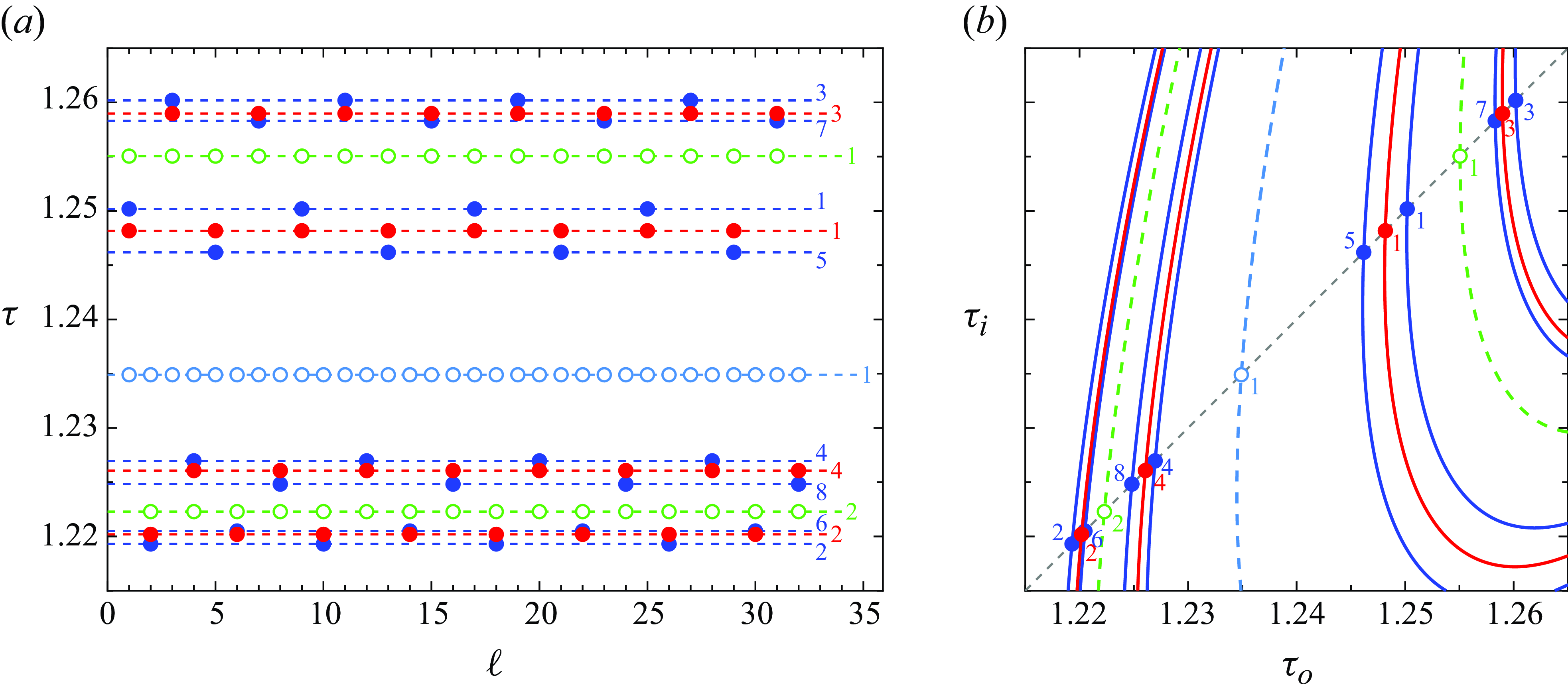
Figure 6. All orbits up to period 8 at (P $_1$
and P
$_1$
and P $_2$
, unstable) and around (P
$_2$
, unstable) and around (P $_4$
and P
$_4$
and P $_8$
, at
$_8$
, at $R=395.711$
and
$R=395.711$
and $395.719$
, respectively) PD
$395.719$
, respectively) PD $_3$
. (a) Torque (
$_3$
. (a) Torque ( $\tau =\tau _i=\tau _o$
) of P
$\tau =\tau _i=\tau _o$
) of P $_1$
(cyan), P
$_1$
(cyan), P $_2$
(green), P
$_2$
(green), P $_4$
(blue) and P
$_4$
(blue) and P $_8$
(red) on
$_8$
(red) on $\Sigma$
as a function of the discrete time
$\Sigma$
as a function of the discrete time $\ell$
(crossing index). The dashed lines indicate the distinct values of
$\ell$
(crossing index). The dashed lines indicate the distinct values of $\tau$
. (b) Two-dimensional phase map projection on the
$\tau$
. (b) Two-dimensional phase map projection on the $(\tau _o,\tau _i)$
plane. Shown are the phase map trajectories of all four orbits (dashed line for unstable, solid for stable) along with their representation on the Poincaré section (circles, open for unstable, filled for stable). The numbers indicate the order of the crossings.
$(\tau _o,\tau _i)$
plane. Shown are the phase map trajectories of all four orbits (dashed line for unstable, solid for stable) along with their representation on the Poincaré section (circles, open for unstable, filled for stable). The numbers indicate the order of the crossings.
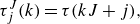
The $n$
th period-doubling bifurcation PD
$n$
th period-doubling bifurcation PD $_n$
can be readily analysed by splitting the
$_n$
can be readily analysed by splitting the $\tau (\ell )$
sequences of interest into
$\tau (\ell )$
sequences of interest into $J=2^n$
separate subsequences
$J=2^n$
separate subsequences
 \begin{equation} \tau _j^J(k)=\tau (kJ+j), \end{equation}
each starting at one of $J$
consecutive Poincaré crossings
$J$
consecutive Poincaré crossings $j\in \{1,\ldots J\}$
, and sampling every
$j\in \{1,\ldots J\}$
, and sampling every $J$
th crossing thereafter. The limits
$J$
th crossing thereafter. The limits
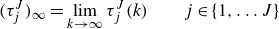 \begin{equation} (\tau _j^J)_\infty = \lim _{k\to \infty }\tau _j^J(k) \qquad j\in \{1,\ldots J\} \end{equation}
exist for all subsequences of all orbits of period $N=J=2^n$
or lower (
$N=J=2^n$
or lower ( $J/2,J/4,\dots$
) along the cascade, but fail for orbits of longer period (
$J/2,J/4,\dots$
) along the cascade, but fail for orbits of longer period ( $2J,4J,\dots$
). Moreover, only period-
$2J,4J,\dots$
). Moreover, only period- $J$
orbits will produce
$J$
orbits will produce $J$
distinct
$J$
distinct $(\tau _j^J)_\infty$
values, while shorter period orbits will have the limits coincide in pairs according to
$(\tau _j^J)_\infty$
values, while shorter period orbits will have the limits coincide in pairs according to $(\tau _j^J)_\infty =(\tau _{j+J/2}^J)_\infty$
. This property is instrumental in telling apart orbits of period
$(\tau _j^J)_\infty =(\tau _{j+J/2}^J)_\infty$
. This property is instrumental in telling apart orbits of period $N=J$
from orbits of period
$N=J$
from orbits of period $J/2$
or smaller, as the amplitudes defined by
$J/2$
or smaller, as the amplitudes defined by
 \begin{equation} A_j^J = \left \lvert (\tau _j^J)_\infty -(\tau _{j+J/2}^J)_\infty \right \rvert \qquad j\in \{1\ldots J/2\}, \end{equation}
will all vanish for any orbit other than P $_J$
. For instance, suppose we slightly perturb the stable P
$_J$
. For instance, suppose we slightly perturb the stable P $_8$
at
$_8$
at $R=395.719$
. If we sample the
$R=395.719$
. If we sample the $\tau$
sequence with
$\tau$
sequence with $J=8$
, all subsequences
$J=8$
, all subsequences $j=1,2,3,\dots ,8$
converge and all eight limits are different (recall figure 6). Applying the same
$j=1,2,3,\dots ,8$
converge and all eight limits are different (recall figure 6). Applying the same $J=8$
sampling to a stable P
$J=8$
sampling to a stable P $_4$
(or P
$_4$
(or P $_2$
or P
$_2$
or P $_1$
) will instead produce indistinguishable limits for
$_1$
) will instead produce indistinguishable limits for $j$
and
$j$
and $j+4$
and, consequently, vanishing amplitudes
$j+4$
and, consequently, vanishing amplitudes $A_j^8=0$
.
$A_j^8=0$
.
To nail down PD $_3$
, a collection of DNS runs traversing the bifurcation point, i.e. between
$_3$
, a collection of DNS runs traversing the bifurcation point, i.e. between $R=395.711$
and
$R=395.711$
and $395.719$
, are required. The amplitude of P
$395.719$
, are required. The amplitude of P $_8$
drops fast as the parameter
$_8$
drops fast as the parameter $R$
is decreased towards PD
$R$
is decreased towards PD $_3$
, such that distinguishing it from P
$_3$
, such that distinguishing it from P $_4$
becomes increasingly difficult. In addition, the dynamics become despairingly slow as the bifurcation point is approached from either side, rendering convergence with DNS downright impracticable. Figures 7(a) and 7(b) depict the torque subsequences at
$_4$
becomes increasingly difficult. In addition, the dynamics become despairingly slow as the bifurcation point is approached from either side, rendering convergence with DNS downright impracticable. Figures 7(a) and 7(b) depict the torque subsequences at $R=395.7116$
and
$R=395.7116$
and $R=395.7122$
, respectively, below and above PD
$R=395.7122$
, respectively, below and above PD $_3$
but moderately close to the bifurcation point. Every pair of sequences (
$_3$
but moderately close to the bifurcation point. Every pair of sequences ( $\tau _j^8$
and
$\tau _j^8$
and $\tau _{j+4}^8$
, depicted in different shades of the same colour) appears to be converging to the same value at
$\tau _{j+4}^8$
, depicted in different shades of the same colour) appears to be converging to the same value at $R=395.7116$
, but not at
$R=395.7116$
, but not at $R=395.7122$
. At these values of
$R=395.7122$
. At these values of $R$
, the achievable degree of convergence is still reasonable but sufficiently slow to illustrate how the estimation of the amplitudes may be systematised to parameter values much closer to the bifurcation point. Well past initial transients, and as the sequences approach convergence, the dynamics is progressively determined by the governing equations linearised around the stable solution. Therefore, we can expect that a power law fit of the form
$R$
, the achievable degree of convergence is still reasonable but sufficiently slow to illustrate how the estimation of the amplitudes may be systematised to parameter values much closer to the bifurcation point. Well past initial transients, and as the sequences approach convergence, the dynamics is progressively determined by the governing equations linearised around the stable solution. Therefore, we can expect that a power law fit of the form
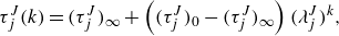 \begin{equation} \tau _j^J(k) =(\tau _j^J)_{\infty }+ \left ((\tau _j^J)_0-(\tau _j^J)_{\infty }\right )(\lambda _j^J)^k, \end{equation}
with fitting parameters $(\tau _j^J)_{\infty }, (\tau _j^J)_0$
and
$(\tau _j^J)_{\infty }, (\tau _j^J)_0$
and $\lambda _j^J$
, conforms reasonably well to the final transients. The fit provides an estimate for both the asymptotic torque value
$\lambda _j^J$
, conforms reasonably well to the final transients. The fit provides an estimate for both the asymptotic torque value $(\tau _j^J)_{\infty }$
and the dominant multiplier
$(\tau _j^J)_{\infty }$
and the dominant multiplier $\lambda _j^J$
. The dashed lines in the insets of the top panels of figure 7 are the fits to the sequences
$\lambda _j^J$
. The dashed lines in the insets of the top panels of figure 7 are the fits to the sequences $\tau _j^J(k)$
,
$\tau _j^J(k)$
, $k\geqslant 0$
. To expose the convergence rate and the accuracy of the fits, the same data have been plotted in the mid panels, now subtracting from each pair of branches
$k\geqslant 0$
. To expose the convergence rate and the accuracy of the fits, the same data have been plotted in the mid panels, now subtracting from each pair of branches $j$
and
$j$
and $j+4$
the mean value
$j+4$
the mean value $((\tau _j^8)_\infty +(\tau _{j+4}^8)_\infty )/2$
at infinity. The fits provide an excellent approximation to the data points because the dynamics has already reached the linear regime. While all fitting curves decay to zero for
$((\tau _j^8)_\infty +(\tau _{j+4}^8)_\infty )/2$
at infinity. The fits provide an excellent approximation to the data points because the dynamics has already reached the linear regime. While all fitting curves decay to zero for $R=395.7116$
in this representation, four distinct amplitudes arise for
$R=395.7116$
in this representation, four distinct amplitudes arise for $R=395.7122$
. This unequivocally identifies the former dynamics as converging on a P
$R=395.7122$
. This unequivocally identifies the former dynamics as converging on a P $_4$
and the latter on a P
$_4$
and the latter on a P $_8$
. The bottom panels plot the same data yet again, but now in logarithmic scale. In this representation, all fits to the individual torque subsequences are seen to collapse onto a single straight line. The eight slopes
$_8$
. The bottom panels plot the same data yet again, but now in logarithmic scale. In this representation, all fits to the individual torque subsequences are seen to collapse onto a single straight line. The eight slopes $\lambda _j^8$
, indistinguishable from one another to the naked eye, provide an estimate to the dominant multiplier of the converging periodic solution, interpreted as a P
$\lambda _j^8$
, indistinguishable from one another to the naked eye, provide an estimate to the dominant multiplier of the converging periodic solution, interpreted as a P $_8$
regardless of its actual period.
$_8$
regardless of its actual period.
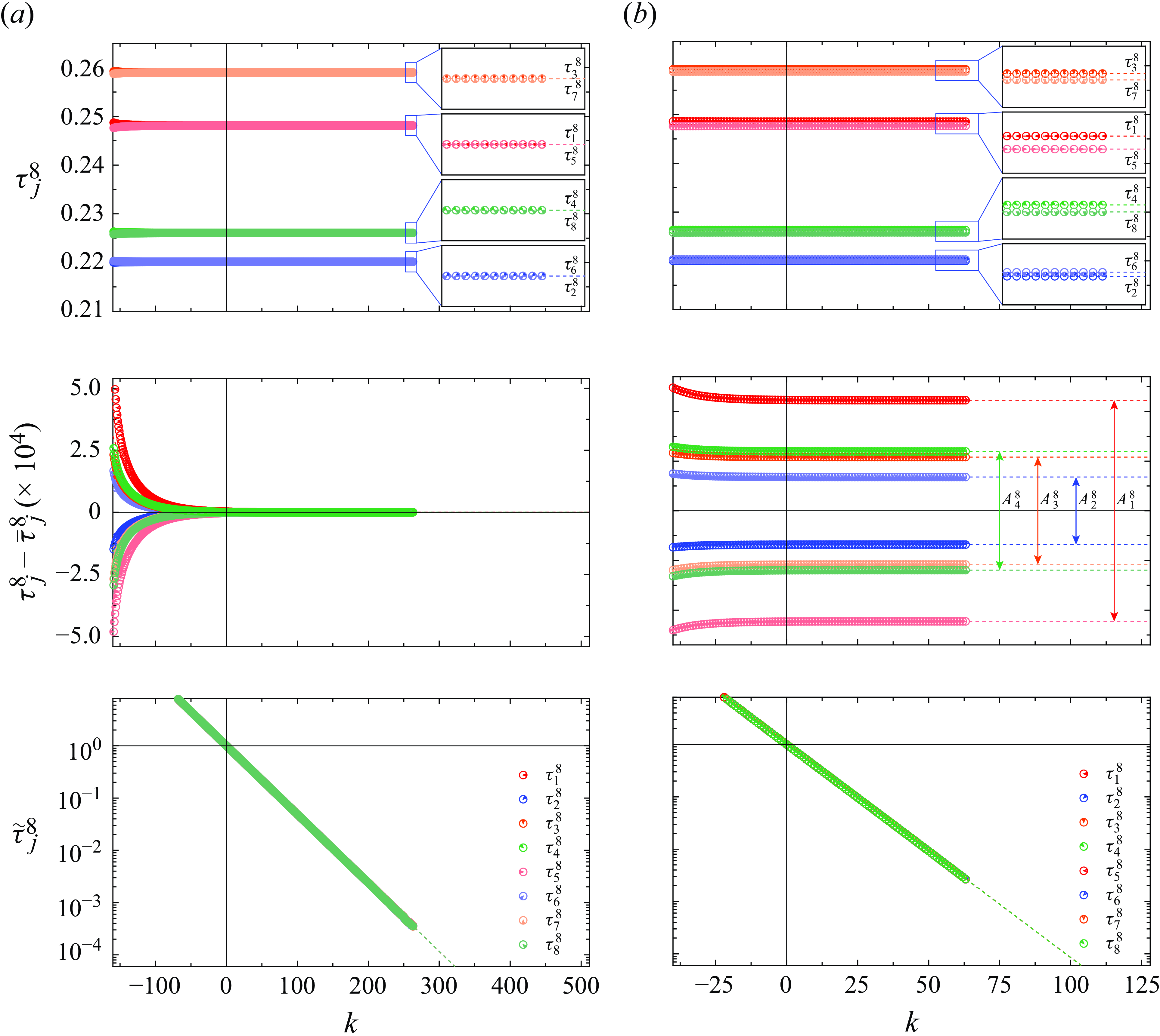
Figure 7. Analysis of torque sequences $\tau (\ell )$
, sampled with
$\tau (\ell )$
, sampled with $N=8$
at (a)
$N=8$
at (a) $R=395.7116$
and (b)
$R=395.7116$
and (b) $R=395.7122$
, below and above PD
$R=395.7122$
, below and above PD $_3$
(
$_3$
( $R=395.711841564$
, as we shall see later), respectively. The top panels show the eight sequences
$R=395.711841564$
, as we shall see later), respectively. The top panels show the eight sequences $\tau _j^8(k)$
(circles, magnified in the insets), alongside respective power law fits (dashed lines). To differentiate the eight subsequences, the points corresponding to each are coloured and represented with disks that are mainly blank except for a 1/8th sector, whose orientation (
$\tau _j^8(k)$
(circles, magnified in the insets), alongside respective power law fits (dashed lines). To differentiate the eight subsequences, the points corresponding to each are coloured and represented with disks that are mainly blank except for a 1/8th sector, whose orientation ( $360^\circ \times j/8$
) uniquely identifies the corresponding sequence
$360^\circ \times j/8$
) uniquely identifies the corresponding sequence $\tau _j^8$
(see the legend). The mid panels show the same data but with the mean value
$\tau _j^8$
(see the legend). The mid panels show the same data but with the mean value $\overline{\tau}_j^8 = [(\tau_j^8)_\infty + (\tau_{j+4}^8)_\infty] /2$
subtracted from every pair of branches to illustrate convergence. The bottom panels show again the same data but in logarithmic scale:
$\overline{\tau}_j^8 = [(\tau_j^8)_\infty + (\tau_{j+4}^8)_\infty] /2$
subtracted from every pair of branches to illustrate convergence. The bottom panels show again the same data but in logarithmic scale: $\tilde{\tau}_j^8 = [\tau_j^8 - (\tau_j^8)_\infty]/[(\tau_j^8)_0 - (\tau_j^8)_\infty]$
.
$\tilde{\tau}_j^8 = [\tau_j^8 - (\tau_j^8)_\infty]/[(\tau_j^8)_0 - (\tau_j^8)_\infty]$
.
The four amplitudes $A_j^8$
and eight multipliers
$A_j^8$
and eight multipliers $\lambda _j^8$
have been computed, following the same procedure with the sampling
$\lambda _j^8$
have been computed, following the same procedure with the sampling $J=8$
, at several values of
$J=8$
, at several values of $R$
approaching PD
$R$
approaching PD $_3$
from either side, and plotted in figure 8. Figure 8(a) indicates that there is a well-defined critical value of
$_3$
from either side, and plotted in figure 8. Figure 8(a) indicates that there is a well-defined critical value of $R$
, beyond which, all four
$R$
, beyond which, all four $A_j^8$
start growing following a square root law, as expected for a period-doubling bifurcation. To accurately pinpoint the critical value of the parameter for PD
$A_j^8$
start growing following a square root law, as expected for a period-doubling bifurcation. To accurately pinpoint the critical value of the parameter for PD $_n$
, a fit of the form
$_n$
, a fit of the form
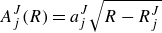 \begin{equation} A_j^J(R) = a_j^J\sqrt {R-R_j^J} \end{equation}
with $J=2^n$
applied to the first few points after the period-doubling bifurcation. The fits provide, besides the
$J=2^n$
applied to the first few points after the period-doubling bifurcation. The fits provide, besides the $a_j^J$
values for the
$a_j^J$
values for the $J/2$
scaling factors,
$J/2$
scaling factors, $J/2$
independent estimates
$J/2$
independent estimates $R_j^J$
for the critical value of the parameter. A unique estimate for the critical value is then obtained by taking the arithmetic mean of the
$R_j^J$
for the critical value of the parameter. A unique estimate for the critical value is then obtained by taking the arithmetic mean of the $J/2$
individual estimates as
$J/2$
individual estimates as $R_n=\langle R_j^J\rangle$
. Performing the
$R_n=\langle R_j^J\rangle$
. Performing the $J/2=4$
fits to the data points of figure 8(a) (dashed lines), yields
$J/2=4$
fits to the data points of figure 8(a) (dashed lines), yields $R_3=\langle R_j^8\rangle =395.71184156\pm 5\times 10^{-8}$
(violet square) for PD
$R_3=\langle R_j^8\rangle =395.71184156\pm 5\times 10^{-8}$
(violet square) for PD $_3$
.
$_3$
.
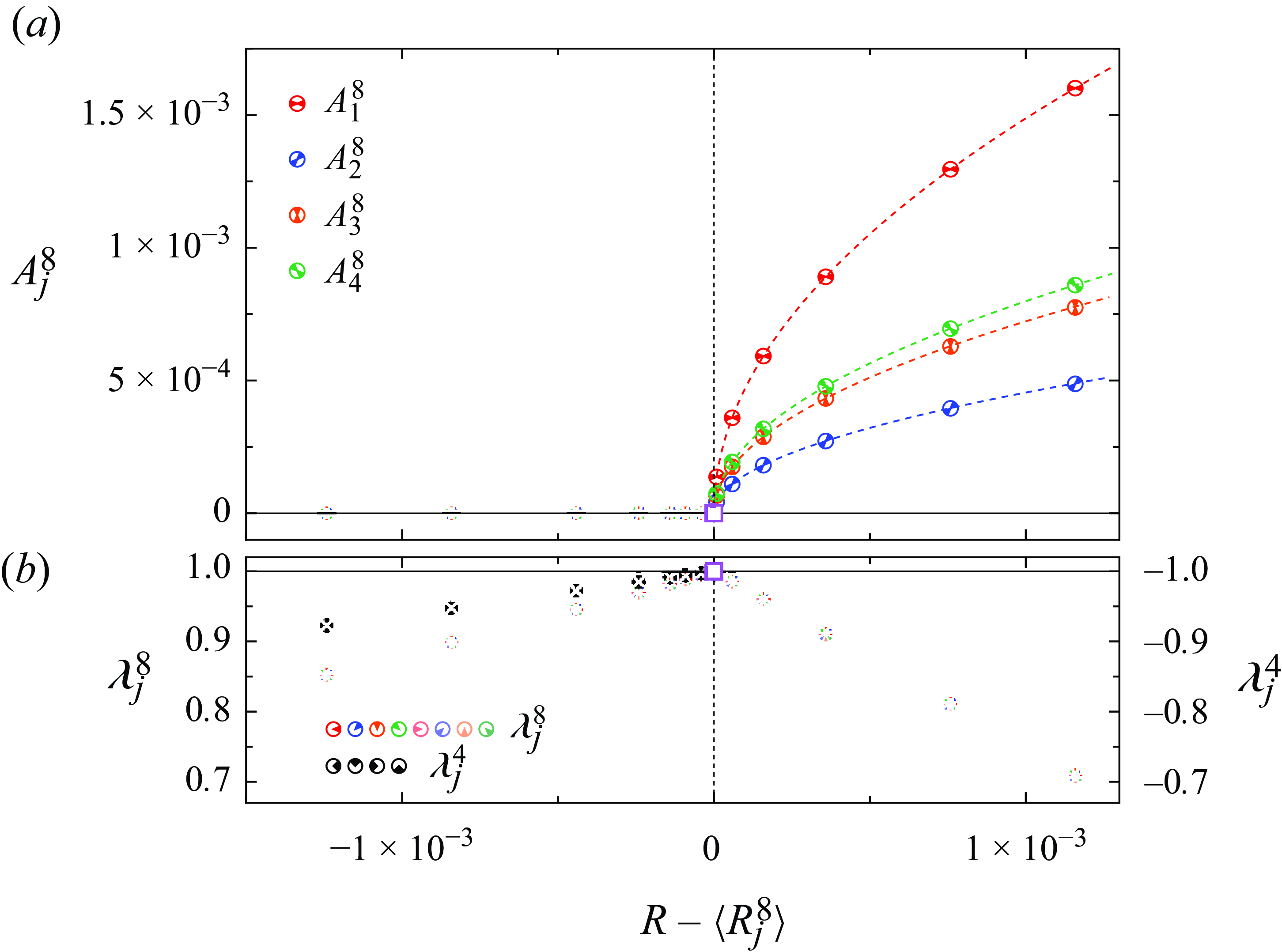
Figure 8. Analysis of PD $_3$
. (a) Torque amplitudes
$_3$
. (a) Torque amplitudes $A_j^8$
and (b) multipliers
$A_j^8$
and (b) multipliers $\lambda _j^8$
(coloured, sampling
$\lambda _j^8$
(coloured, sampling $\tau (\ell )$
with
$\tau (\ell )$
with $N=8$
) and
$N=8$
) and $\lambda _j^4$
(black, sampling with
$\lambda _j^4$
(black, sampling with $N=4$
), as a function of inner cylinder Reynolds number
$N=4$
), as a function of inner cylinder Reynolds number $R-\langle R_j^8\rangle$
. The square-root fits are indicated with dashed lines. The lower bounds for the uncertainty of each point, shown as error bars, are sufficiently small to be imperceptible. Following the graphical representation of the
$R-\langle R_j^8\rangle$
. The square-root fits are indicated with dashed lines. The lower bounds for the uncertainty of each point, shown as error bars, are sufficiently small to be imperceptible. Following the graphical representation of the $\tau _j^8$
sequences of figure 7, each of the amplitudes is represented with a double-sectored disk that results from the superposition of the oppositely oriented sectored disks of the two torques that define the amplitude, hence the hourglass appearance of the symbols.
$\tau _j^8$
sequences of figure 7, each of the amplitudes is represented with a double-sectored disk that results from the superposition of the oppositely oriented sectored disks of the two torques that define the amplitude, hence the hourglass appearance of the symbols.
The eight $\lambda _j^8$
multipliers, shown in figure 8(b), behave as expected across a period-doubling bifurcation. The eight individual fits (3.4) to the eight individual
$\lambda _j^8$
multipliers, shown in figure 8(b), behave as expected across a period-doubling bifurcation. The eight individual fits (3.4) to the eight individual $\tau _j^8$
subsequences produce nearly identical values of
$\tau _j^8$
subsequences produce nearly identical values of $\lambda _j^8$
at any given
$\lambda _j^8$
at any given $R$
, hence the multicoloured filled circles, resulting from the superposition of the eight oriented sectored disks. The unique estimate of the multiplier at any given
$R$
, hence the multicoloured filled circles, resulting from the superposition of the eight oriented sectored disks. The unique estimate of the multiplier at any given $R$
, obtained as the arithmetic mean
$R$
, obtained as the arithmetic mean $\lambda _8=\langle \lambda _j^8\rangle$
, increases towards unity as the period-doubling point is approached from either side. Since the solution above PD
$\lambda _8=\langle \lambda _j^8\rangle$
, increases towards unity as the period-doubling point is approached from either side. Since the solution above PD $_3$
is indeed a P
$_3$
is indeed a P $_8$
,
$_8$
, $\lambda _8$
is directly its multiplier. This is not so for the P
$\lambda _8$
is directly its multiplier. This is not so for the P $_4$
solution below PD
$_4$
solution below PD $_3$
. Plots analogous to those in figure 7(a) but sampling with
$_3$
. Plots analogous to those in figure 7(a) but sampling with $J=4$
show that convergence onto the four asymptotic branches follows an oscillatory pattern. The multiplier of the P
$J=4$
show that convergence onto the four asymptotic branches follows an oscillatory pattern. The multiplier of the P $_4$
orbit in the vicinity of PD
$_4$
orbit in the vicinity of PD $_3$
must be either computed from fits to the torque subsequences sampled with
$_3$
must be either computed from fits to the torque subsequences sampled with $J=4$
or indirectly from
$J=4$
or indirectly from $\lambda _8$
according to
$\lambda _8$
according to $\lambda _4=\langle \lambda _j^4\rangle =-\sqrt {\lambda _8}$
. Either way, the multiplier of the stable P
$\lambda _4=\langle \lambda _j^4\rangle =-\sqrt {\lambda _8}$
. Either way, the multiplier of the stable P $_4$
in the vicinity of PD
$_4$
in the vicinity of PD $_3$
is real, negative and on the way of leaving the unit circle of the complex plane through
$_3$
is real, negative and on the way of leaving the unit circle of the complex plane through $\lambda =-1$
as
$\lambda =-1$
as $R_3$
is approached from below (black disks in figure 8
b), consistent with the period-doubling nature of the bifurcation.
$R_3$
is approached from below (black disks in figure 8
b), consistent with the period-doubling nature of the bifurcation.
4. Verification of Feigenbaum universality
Signs that the period-doubling cascade may exhibit some sort of universality are already apparent from figure 9, where all orbits computed up to period $N=128$
(past PD
$N=128$
(past PD $_7$
) are shown as a function of
$_7$
) are shown as a function of $R$
. Successive magnifications, presented in figures 9(b) and 9(c), exhibit branch structures very similar to that of the full cascade of figure 9(a). Yet, at this stage, there is no guarantee that the universality observed here is of the same kind as discovered by Feigenbaum.
$R$
. Successive magnifications, presented in figures 9(b) and 9(c), exhibit branch structures very similar to that of the full cascade of figure 9(a). Yet, at this stage, there is no guarantee that the universality observed here is of the same kind as discovered by Feigenbaum.

Figure 9. Successive magnifications of the period-doubling cascade. Same data as in figure 5(b), truncated at the accumulation point $R_{\infty }$
, the central branch indicated with black dots. (a) Overview and (b,c)two successive levels of magnification. The first few period-doubling bifurcations (
$R_{\infty }$
, the central branch indicated with black dots. (a) Overview and (b,c)two successive levels of magnification. The first few period-doubling bifurcations ( $R_n$
, dashed) and the accumulation point (
$R_n$
, dashed) and the accumulation point ( $R_\infty$
, solid) are indicated with grey lines and labels.
$R_\infty$
, solid) are indicated with grey lines and labels.
To ascertain Feigenbaum universality, we have computed the sequence of critical $R_n$
values along the period-doubling cascade up to order
$R_n$
values along the period-doubling cascade up to order $n=7$
to very high accuracy, using the method described in § 3.2. The results are summarised in table 2. For every
$n=7$
to very high accuracy, using the method described in § 3.2. The results are summarised in table 2. For every $n\geqslant 3$
, the table also lists the ratios
$n\geqslant 3$
, the table also lists the ratios $\delta _n$
, defined as
$\delta _n$
, defined as
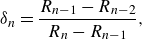 \begin{equation} \delta _n = \dfrac {R_{n-1}-R_{n-2}}{R_{n}-R_{n-1}}, \end{equation}
which provide the best approximation to Feigenbaum’s first constant $\delta _{{F}}$
that may be obtained from data up to the
$\delta _{{F}}$
that may be obtained from data up to the $n$
th period doubling. The trend of
$n$
th period doubling. The trend of $\delta _n$
exhibits evident signs of conforming to Feigenbaum universality, that is,
$\delta _n$
exhibits evident signs of conforming to Feigenbaum universality, that is, $\delta _n \rightarrow \delta _{{F}}$
as
$\delta _n \rightarrow \delta _{{F}}$
as $n\rightarrow \infty$
. It is instructive to compare these results with those in table 1. Limiting the analysis to
$n\rightarrow \infty$
. It is instructive to compare these results with those in table 1. Limiting the analysis to $n=4$
, as customarily done in the fluid dynamics literature, does not guarantee convergence to even the second significant digit. Securing three digits precision is an arduous task that typically requires the accurate determination of at least
$n=4$
, as customarily done in the fluid dynamics literature, does not guarantee convergence to even the second significant digit. Securing three digits precision is an arduous task that typically requires the accurate determination of at least $n=7$
period-doubling bifurcation points.
$n=7$
period-doubling bifurcation points.
Table 2. Confirmation of Feigenbaum universality along the period-doubling cascade. The values of the critical inner cylinder Reynolds number $R_n$
at the
$R_n$
at the $n$
th period doubling bifurcation point PD
$n$
th period doubling bifurcation point PD $_n$
are used to compute the
$_n$
are used to compute the $n$
th approximation,
$n$
th approximation, $\delta _n$
, to Feigenbaum’s first constant, according to (4.1). Approximations,
$\delta _n$
, to Feigenbaum’s first constant, according to (4.1). Approximations, $\alpha _n$
, to the second constant, are computed from central branch torque values following (4.8). Lower bounds to the uncertainties in the
$\alpha _n$
, to the second constant, are computed from central branch torque values following (4.8). Lower bounds to the uncertainties in the $R_n$
,
$R_n$
, $\delta _n$
,
$\delta _n$
, $\alpha _n$
and
$\alpha _n$
and $R_\infty$
parameters have been rigorously estimated from the covariance matrices of the various fits involved in the process, combined with standard error propagation theory (note that we have not taken into account the error of the fit (3.4), as conducting a systematic study is difficult). The last row of the table corresponds to the accumulation point
$R_\infty$
parameters have been rigorously estimated from the covariance matrices of the various fits involved in the process, combined with standard error propagation theory (note that we have not taken into account the error of the fit (3.4), as conducting a systematic study is difficult). The last row of the table corresponds to the accumulation point $R_{\infty }$
estimated by (4.7), and the actual values of Feigenbaum constants,
$R_{\infty }$
estimated by (4.7), and the actual values of Feigenbaum constants, $\delta _{{F}}$
and
$\delta _{{F}}$
and $\alpha _{{F}}$
.
$\alpha _{{F}}$
.

The $R_n$
sequence is expected to converge onto the accumulation point,
$R_n$
sequence is expected to converge onto the accumulation point, $R=R_\infty$
. This point may be computed by assuming that all period-doubling bifurcations of order higher than available are perfectly Feigenbaum-universal and, therefore, satisfy (4.1) with the left-hand side replaced by
$R=R_\infty$
. This point may be computed by assuming that all period-doubling bifurcations of order higher than available are perfectly Feigenbaum-universal and, therefore, satisfy (4.1) with the left-hand side replaced by $\delta _{{F}}$
. However, this naive approach leads to systematic error. To obtain a better estimate of
$\delta _{{F}}$
. However, this naive approach leads to systematic error. To obtain a better estimate of $R_{\infty }$
and, at the same time, bound the error, we first note that
$R_{\infty }$
and, at the same time, bound the error, we first note that
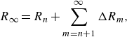 \begin{eqnarray} R_{\infty } = R_n+\sum _{m=n+1}^{\infty }{\Delta R_m}, \end{eqnarray}
where $\Delta R_m\equiv R_m-R_{m-1}$
denotes the interval between the
$\Delta R_m\equiv R_m-R_{m-1}$
denotes the interval between the $(m-1)$
and
$(m-1)$
and $m$
th period-doubling bifurcations. Since (4.1) can be written as
$m$
th period-doubling bifurcations. Since (4.1) can be written as $\delta _n=\Delta R_{n-1}/\Delta R_{n}$
, any successive
$\delta _n=\Delta R_{n-1}/\Delta R_{n}$
, any successive $m$
th interval may be expressed recursively in terms of previous intervals as
$m$
th interval may be expressed recursively in terms of previous intervals as
 \begin{equation} \Delta R_{m}=\delta _m^{-1}\Delta R_{m-1}=\delta _m^{-1}\delta _{m-1}^{-1}\Delta R_{m-2}=\dots =\delta _m^{-1}\delta _{m-1}^{-1}\cdots \delta _{n+1}^{-1}\Delta R_{n}=\Delta R_{n}\prod _{\ell =n+1}^{m}\delta _\ell ^{-1}. \end{equation}
The accumulation point can then be formally expressed in terms of the n $th$
period doubling and the immediately preceding interval as
$th$
period doubling and the immediately preceding interval as
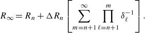 \begin{eqnarray} R_{\infty } = R_n+\Delta R_n\left [\sum _{m=n+1}^{\infty }{\prod _{\ell =n+1}^{m}\delta _\ell ^{-1}}\right ]. \end{eqnarray}
If $\delta _\ell =\tilde {\delta }_n\gt 1$
were constant for all
$\delta _\ell =\tilde {\delta }_n\gt 1$
were constant for all $ \ell \gt n$
, then the terms in the square brackets would form a geometric series of sum
$ \ell \gt n$
, then the terms in the square brackets would form a geometric series of sum $1/(\tilde {\delta }_n-1)$
. We conveniently define the average ratio beyond PD
$1/(\tilde {\delta }_n-1)$
. We conveniently define the average ratio beyond PD $_n$
as
$_n$
as
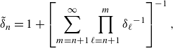 \begin{equation} \tilde {\delta }_n = 1 + \left [ \sum _{m=n+1}^{\infty }\displaystyle {\prod _{\ell =n+1}^{m}{\delta _\ell }^{-1}} \right ]^{-1}, \end{equation}
so that (4.4) simplifies to
 \begin{equation} R_\infty = R_n + \dfrac {\Delta R_n}{\tilde {\delta }_n-1} = \dfrac {\tilde {\delta }_n R_n - R_{n-1}}{\tilde {\delta }_n-1}. \end{equation}
The constant $\tilde {\delta }_n$
is unknown and may only be estimated. For
$\tilde {\delta }_n$
is unknown and may only be estimated. For $n$
sufficiently large, the sequence
$n$
sufficiently large, the sequence $\delta _\ell$
for all
$\delta _\ell$
for all $\ell \gt n$
is expected to approach
$\ell \gt n$
is expected to approach $\delta _{{F}}$
monotonically from above. Under this assumption, inspection of (4.5) provides the inequalities
$\delta _{{F}}$
monotonically from above. Under this assumption, inspection of (4.5) provides the inequalities $\delta _{{F}}\lt \delta _{n+1}\lt \tilde {\delta }_n \lt \delta _n$
. Accordingly, upper and lower bounds for
$\delta _{{F}}\lt \delta _{n+1}\lt \tilde {\delta }_n \lt \delta _n$
. Accordingly, upper and lower bounds for $R_\infty$
can be obtained as
$R_\infty$
can be obtained as
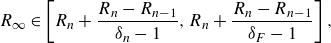 \begin{equation} R_\infty \in \left [R_n+\dfrac {R_n-R_{n-1}}{\delta _n-1},R_n+\dfrac {R_n-R_{n-1}}{\delta _{{F}}-1}\right ], \end{equation}
by substituting $\tilde {\delta }_n=\delta _n$
and
$\tilde {\delta }_n=\delta _n$
and $\tilde {\delta }_n=\delta _{{F}}$
in (4.6), respectively. Using PD
$\tilde {\delta }_n=\delta _{{F}}$
in (4.6), respectively. Using PD $_7$
, the upper and lower bounds for
$_7$
, the upper and lower bounds for $R_\infty$
are already within the uncertainty range of one another (see table 2) and, combined, provide an accurate estimate for the accumulation point
$R_\infty$
are already within the uncertainty range of one another (see table 2) and, combined, provide an accurate estimate for the accumulation point $R_\infty =395.721266624\pm 1.1\times 10^{-8}$
.
$R_\infty =395.721266624\pm 1.1\times 10^{-8}$
.
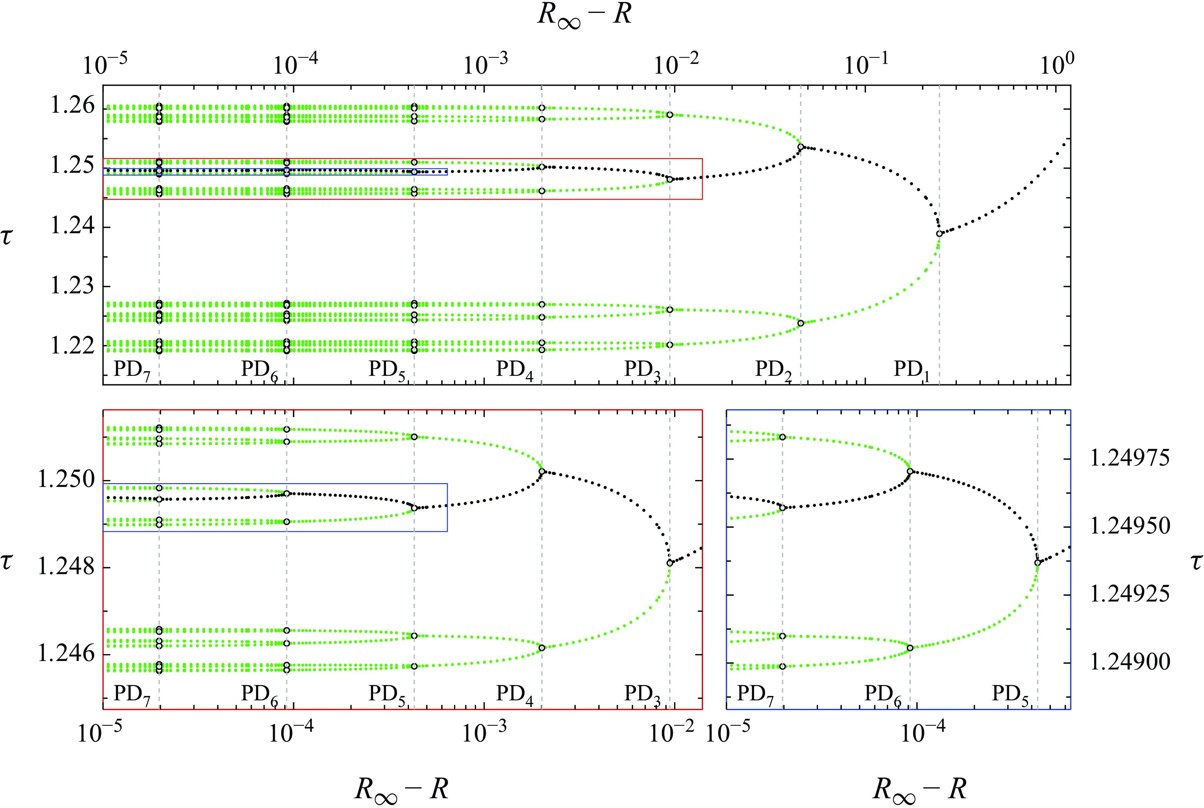
Figure 10. Self-similarity of the period-doubling cascade. Same data as figure 9 in log scale, the central branch represented with black dots. The coloured bottom panels are successive magnifications of the boxes in the top panel. The bifurcations are indicated with dashed vertical lines and labelled PD $_n$
according to their order.
$_n$
according to their order.
Following the determination of the accumulation point, we can now plot the period-doubling cascade as a function of $R_\infty -R$
in logarithmic scale (figure 10). The asymptotic approach to universality and the accuracy with which the accumulation point has been obtained are evident from the similarities observed after two consecutive magnifications of the period-doubling cascade (red and blue bottom panels).
$R_\infty -R$
in logarithmic scale (figure 10). The asymptotic approach to universality and the accuracy with which the accumulation point has been obtained are evident from the similarities observed after two consecutive magnifications of the period-doubling cascade (red and blue bottom panels).
The occurrence of Feigenbaum universality implies that the dynamics of the Navier–Stokes system is governed by a (nearly) one-dimensional discrete map. Figure 11(a) depicts a three-dimensional phase map projection of the orbit at the accumulation point $R_\infty$
. If the manifold has dimension one, the coefficients
$R_\infty$
. If the manifold has dimension one, the coefficients $\mathbf {a}$
on the Poincaré section
$\mathbf {a}$
on the Poincaré section $\Sigma$
introduced in (2.10) can be uniquely parametrised by the torque, such that the first return map
$\Sigma$
introduced in (2.10) can be uniquely parametrised by the torque, such that the first return map $f$
defined by
$f$
defined by $\tau (\ell +1)=f(\tau (\ell ))$
contains all the long-term properties of the Poincaré map. The aperiodicity of the orbit becomes apparent when plotting
$\tau (\ell +1)=f(\tau (\ell ))$
contains all the long-term properties of the Poincaré map. The aperiodicity of the orbit becomes apparent when plotting $\tau (\ell +1)$
as a function of
$\tau (\ell +1)$
as a function of $\tau (\ell )$
(green dots in figure 11
b). The structure of the map on
$\tau (\ell )$
(green dots in figure 11
b). The structure of the map on $\Sigma$
is, however, not clear, as the
$\Sigma$
is, however, not clear, as the $\Sigma$
-crossings of the orbit are sparsely distributed (see figure 11
a). Perturbing the orbit, dropping the first initial transients and plotting the remainder of the transients conveniently assists in populating the map more densely (black points). All the points thus obtained fall within a narrow, nearly one-dimensional band, seemingly connected by a smooth curve. This indicates that the discrete-time dynamics on
$\Sigma$
-crossings of the orbit are sparsely distributed (see figure 11
a). Perturbing the orbit, dropping the first initial transients and plotting the remainder of the transients conveniently assists in populating the map more densely (black points). All the points thus obtained fall within a narrow, nearly one-dimensional band, seemingly connected by a smooth curve. This indicates that the discrete-time dynamics on $\Sigma$
in the vicinity of the accumulation point can be well approximated by a one-dimensional map
$\Sigma$
in the vicinity of the accumulation point can be well approximated by a one-dimensional map $f$
. Note that, in the range of
$f$
. Note that, in the range of $\tau$
for which
$\tau$
for which $f$
appears to be multivalued (see the black points), the lower branch is never visited by the attractor and can, therefore, be ignored as regards its dynamics. Accordingly, the function
$f$
appears to be multivalued (see the black points), the lower branch is never visited by the attractor and can, therefore, be ignored as regards its dynamics. Accordingly, the function $f$
, with its leftmost branch duly trimmed, becomes unimodal and its smooth extremum (the minimum) admits a quadratic approximation. Note that unimodal maps with non-quadratic extrema provide universality constants that deviate from Feigenbaum’s well-known values (Briggs Reference Briggs1991).
$f$
, with its leftmost branch duly trimmed, becomes unimodal and its smooth extremum (the minimum) admits a quadratic approximation. Note that unimodal maps with non-quadratic extrema provide universality constants that deviate from Feigenbaum’s well-known values (Briggs Reference Briggs1991).
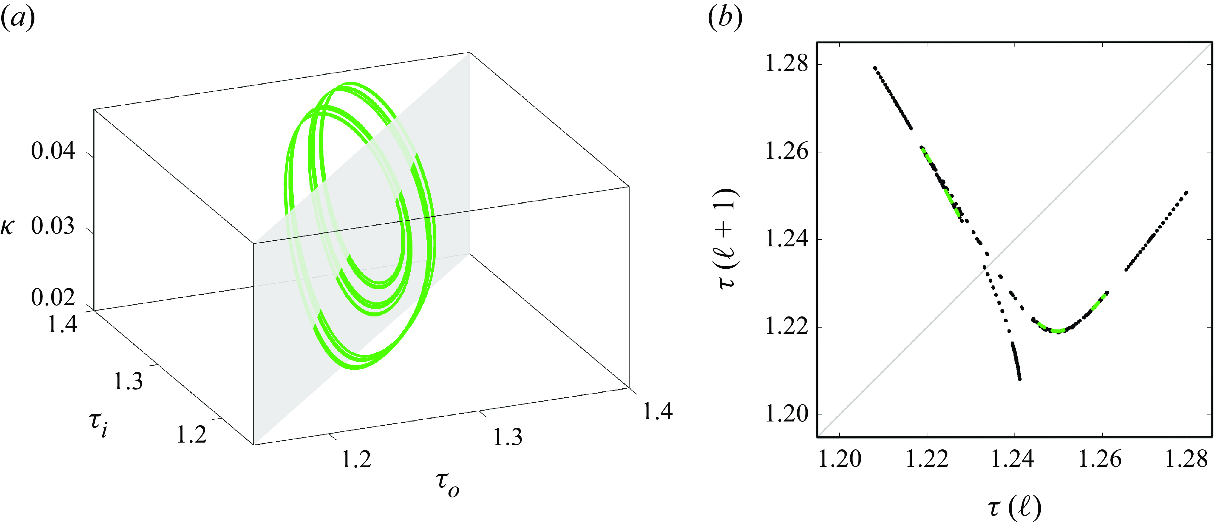
Figure 11. Phase portrait at $R_{\infty }$
. (a) Three-dimensional phase map projection of the chaotic attractor. (b) First return iteration map on
$R_{\infty }$
. (a) Three-dimensional phase map projection of the chaotic attractor. (b) First return iteration map on $\Sigma$
populated by the chaotic attractor (green dots) and transients leading back to it following a perturbation (black).
$\Sigma$
populated by the chaotic attractor (green dots) and transients leading back to it following a perturbation (black).
For period-doubling cascades in one-dimensional unimodal maps, approximations of the second Feigenbaum constant, $\alpha _{{F}}$
, are often obtained from the central branch of the bifurcation diagram, which is generated by the periodic point that is nearest to the extremum of the map. Since producing accurate bifurcation diagrams of cascades undergone by fluid flow systems is an arduous task, Feigenbaum (Reference Feigenbaum1979) used instead the frequency spectrum, recorded at a fixed value of the parameter, of a natural convection experiment. In the subsequent studies summarised in table 1, no evaluation of agreement with
$\alpha _{{F}}$
, are often obtained from the central branch of the bifurcation diagram, which is generated by the periodic point that is nearest to the extremum of the map. Since producing accurate bifurcation diagrams of cascades undergone by fluid flow systems is an arduous task, Feigenbaum (Reference Feigenbaum1979) used instead the frequency spectrum, recorded at a fixed value of the parameter, of a natural convection experiment. In the subsequent studies summarised in table 1, no evaluation of agreement with $\alpha _{{F}}$
was conducted.
$\alpha _{{F}}$
was conducted.
However, we have a highly accurate bifurcation diagram available, rendering direct assessment of agreement with the second constant possible. In the torque sequences presented so far, we have indexed the $N$
distinct points visited by every periodic solution P
$N$
distinct points visited by every periodic solution P $_N$
as
$_N$
as $j=1,2,\dots N$
such that
$j=1,2,\dots N$
such that $j=1$
is the central branch point (the black dots in figure 10). Thus, using the torque values of the central branch at PD
$j=1$
is the central branch point (the black dots in figure 10). Thus, using the torque values of the central branch at PD $_m$
,
$_m$
, $\hat {\tau }_{m}=\tau _1^{2^m}(R_m)$
, we can compute the ratios
$\hat {\tau }_{m}=\tau _1^{2^m}(R_m)$
, we can compute the ratios
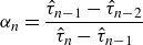 \begin{eqnarray} \alpha _n = \dfrac {\hat {\tau }_{n-1}-\hat {\tau }_{n-2}}{\hat {\tau }_{n}-\hat {\tau }_{n-1}} \end{eqnarray}
to be compared against the $\alpha _{{F}}$
appearing in the Feigenbaum–Cvitanović functional equation. The values of
$\alpha _{{F}}$
appearing in the Feigenbaum–Cvitanović functional equation. The values of $\alpha _n$
thus obtained from the bifurcation diagram, listed in table 2 alongside
$\alpha _n$
thus obtained from the bifurcation diagram, listed in table 2 alongside $\delta _n$
, evidence gradual convergence toward Feigenbaum universality.
$\delta _n$
, evidence gradual convergence toward Feigenbaum universality.
5. Prediction of the period-doubling route to chaos
Following the seminal work of Feigenbaum (Reference Feigenbaum1979), who showcased the first comparison with experimental results, Feigenbaum (Reference Feigenbaum1980, Reference Feigenbaum1982, Reference Feigenbaum1983 Reference Feigenbaum) further extended renormalisation theory to include the universal scaling of all periodic points, not limited to the central branch, at different values of the parameter. The trajectory scaling function theory, which unravels the scaling between orbits featuring the same stability properties (i.e. having the same multiplier), was later applied to interpret experimental data on natural convection by Belmonte et al. (Reference Belmonte, Vinson, Glazier, Gunaratne and Kenny1988).
The occurrence of universality entails that, for any given unimodal map, one should be able to predict the entire structure of the bifurcation diagram near the accumulation point using data from only the initial few period-doubling bifurcations. Unfortunately, the trajectory scaling function method does not provide an easy way to predict the bifurcation cascade. Moreover, orbits become aperiodic beyond the accumulation point, hindering direct comparison with orbits at different parameter values. In this section, we devise a method for predicting the unfolding of the bifurcation cascade up to and beyond the accumulation point.
Consider a general one-dimensional discrete-time dynamical system described by
 \begin{eqnarray} x_{\ell +1}=f_{a}(x_\ell ). \end{eqnarray}
We assume that the function $f_{a}(x)$
is unimodal and that a fixed point of the system (5.1) undergoes a period-doubling cascade as the parameter
$f_{a}(x)$
is unimodal and that a fixed point of the system (5.1) undergoes a period-doubling cascade as the parameter $a$
is increased. In drawing parallels with our Navier–Stokes problem, we will later identify
$a$
is increased. In drawing parallels with our Navier–Stokes problem, we will later identify $a$
and
$a$
and $f_a$
with the Reynolds number
$f_a$
with the Reynolds number $R$
and the function approximating the return map of the torque sequence, respectively. Our claim, motivated by Feigenbaum (Reference Feigenbaum1982), is that the approximation
$R$
and the function approximating the return map of the torque sequence, respectively. Our claim, motivated by Feigenbaum (Reference Feigenbaum1982), is that the approximation
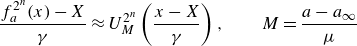 \begin{eqnarray} \frac {f^{2^{n}}_{a}(x)-X}{\gamma } \approx U^{2^n}_{M} \left ( \frac {x-X}{\gamma } \right ), \qquad M= \frac {a-a_{\infty }}{\mu } \end{eqnarray}
holds as long as $2^n$
is sufficiently large,
$2^n$
is sufficiently large,
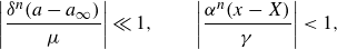 \begin{eqnarray} \left |\frac {\delta ^{n} (a-a_{\infty })}{\mu } \right |\ll 1, \qquad \left | \frac {\alpha ^n(x-X)}{\gamma } \right | \lt 1, \end{eqnarray}
and provided the constants $\gamma$
,
$\gamma$
, $X$
,
$X$
, $\mu$
and
$\mu$
and $a_{\infty }$
are suitably chosen. The derivation of (5.2) and (5.3) is given in Appendix. To simplify the notation, we use functional powers to denote repeated application of a function (e.g.
$a_{\infty }$
are suitably chosen. The derivation of (5.2) and (5.3) is given in Appendix. To simplify the notation, we use functional powers to denote repeated application of a function (e.g. $f^2_a(x)=f_a(f_a(x))$
). Also, we have dropped the F subscript when referring to Feigenbaum’s first (
$f^2_a(x)=f_a(f_a(x))$
). Also, we have dropped the F subscript when referring to Feigenbaum’s first ( $\delta$
) and second (
$\delta$
) and second ( $\alpha$
) constants.
$\alpha$
) constants.
Here, the function $U_M$
appearing in the approximation (5.2) is defined in terms of the Feigenbaum function
$U_M$
appearing in the approximation (5.2) is defined in terms of the Feigenbaum function $G$
and the Feigenfunction
$G$
and the Feigenfunction $\varPhi$
(with the normalisation
$\varPhi$
(with the normalisation $\varPhi (0)=1$
) as
$\varPhi (0)=1$
) as
 \begin{eqnarray} U_M(\xi ) = G(\xi )+M\varPhi (\xi ). \end{eqnarray}
The $\delta$
and
$\delta$
and $\varPhi$
satisfy the eigenvalue problem
$\varPhi$
satisfy the eigenvalue problem $\mathcal {L}_G[\varPhi ]=\delta \varPhi$
. The precise form of the linear operator
$\mathcal {L}_G[\varPhi ]=\delta \varPhi$
. The precise form of the linear operator $\mathcal {L}_G$
is given in Appendix. The nature of
$\mathcal {L}_G$
is given in Appendix. The nature of $G$
and
$G$
and $\varPhi$
is well understood (Collet & Eckmann Reference Collet and Eckmann1980; Briggs Reference Briggs1991; Thurlby Reference Thurlby2021). For our purposes, it will suffice to know that they are both smooth even functions, and that numerical recipes for their computation abound in the literature.
$\varPhi$
is well understood (Collet & Eckmann Reference Collet and Eckmann1980; Briggs Reference Briggs1991; Thurlby Reference Thurlby2021). For our purposes, it will suffice to know that they are both smooth even functions, and that numerical recipes for their computation abound in the literature.
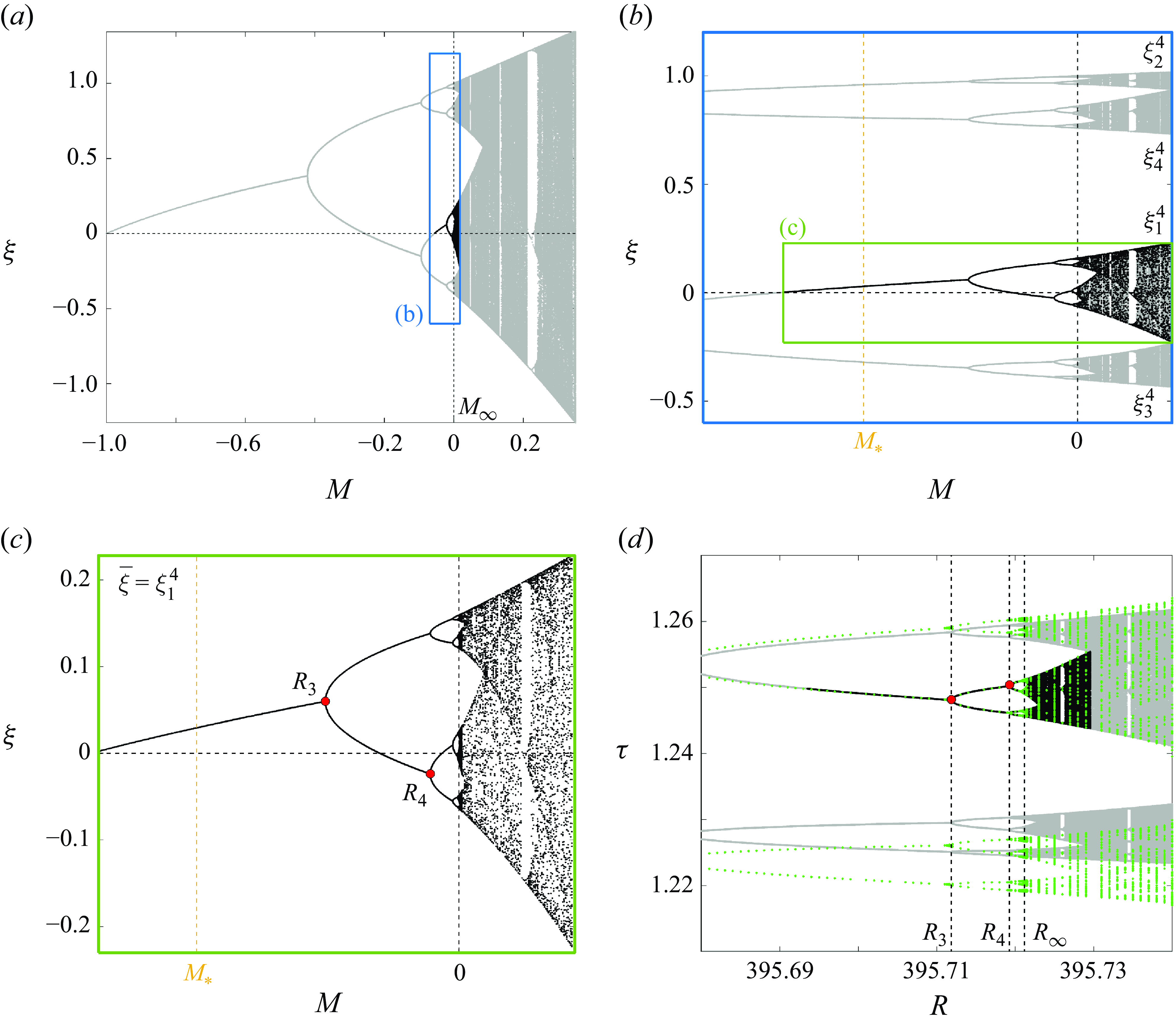
Figure 12. Bifurcation diagram of the one-dimensional map (5.5). (a) Full period-doubling cascade. (b) Magnification around the accumulation point $M_\infty$
. The
$M_\infty$
. The $2^n=4$
distinct sets of points arising for
$2^n=4$
distinct sets of points arising for $M\gt M_*$
are labelled as
$M\gt M_*$
are labelled as $\xi _j^n$
,
$\xi _j^n$
, $j=1,2,3,4$
. Black dots are used for the central branch, grey for the rest. (c) Close-up of the central branch
$j=1,2,3,4$
. Black dots are used for the central branch, grey for the rest. (c) Close-up of the central branch $\overline {\xi }=\xi _1^n$
. The red bullets at PD
$\overline {\xi }=\xi _1^n$
. The red bullets at PD $_3$
and PD
$_3$
and PD $_4$
are the points
$_4$
are the points $(M,\xi )=(M_{n+1},\hat {\xi }_{n+1})$
and
$(M,\xi )=(M_{n+1},\hat {\xi }_{n+1})$
and $(M_{n+2},\hat {\xi }_{n+2})$
selected for the matching with DNS data. (d) Full cascade transformed by (5.8) with
$(M_{n+2},\hat {\xi }_{n+2})$
selected for the matching with DNS data. (d) Full cascade transformed by (5.8) with $(\gamma ,X,\mu ,a_{\infty })$
obtained by (5.7), compared with the period-doubling cascade in Taylor–Couette flow (green dots).
$(\gamma ,X,\mu ,a_{\infty })$
obtained by (5.7), compared with the period-doubling cascade in Taylor–Couette flow (green dots).
If the four (map-dependent) parameters, $\gamma$
,
$\gamma$
, $X$
,
$X$
, $\mu$
and
$\mu$
and $a_{\infty }$
, can be computed from the first few period doublings, then (5.2) provides a useful tool for predicting the behaviour of the dynamical system (5.1), subject to the constraints outlined by (5.3). In practice, fixing
$a_{\infty }$
, can be computed from the first few period doublings, then (5.2) provides a useful tool for predicting the behaviour of the dynamical system (5.1), subject to the constraints outlined by (5.3). In practice, fixing $n=2$
and using data up to PD
$n=2$
and using data up to PD $_{n+2}$
(i.e. PD
$_{n+2}$
(i.e. PD $_4$
) yields already reasonably accurate results. The procedure for prediction is straightforward, as we shall see shortly. All it takes is extracting template branches from the bifurcation diagram of the one-dimesnional dynamical system
$_4$
) yields already reasonably accurate results. The procedure for prediction is straightforward, as we shall see shortly. All it takes is extracting template branches from the bifurcation diagram of the one-dimesnional dynamical system
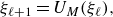 \begin{eqnarray} \xi _{\ell +1}=U_M(\xi _\ell ), \end{eqnarray}
and then stretch and translate them to align with corresponding branches of the bifurcation diagram of (5.1). The constants $X$
and
$X$
and $\gamma$
translate and scale the state
$\gamma$
translate and scale the state $x$
, while
$x$
, while $a_\infty$
and
$a_\infty$
and $\mu$
do the same for the parameter
$\mu$
do the same for the parameter $a$
. The constant
$a$
. The constant $a_{\infty }$
corresponds to the predicted accumulation point of the dynamical system (5.1). Thus, the first condition in (5.3) requires that the parameter
$a_{\infty }$
corresponds to the predicted accumulation point of the dynamical system (5.1). Thus, the first condition in (5.3) requires that the parameter $a$
be sufficiently close to the accumulation point. Likewise,
$a$
be sufficiently close to the accumulation point. Likewise, $X$
corresponds to the predicted position of the extremum of the map
$X$
corresponds to the predicted position of the extremum of the map $f_a(x)$
at
$f_a(x)$
at $a=a_{\infty }$
, and hence the second condition in (5.3) limits the validity of the approximation to a close neighbourhood of the extremum of the map
$a=a_{\infty }$
, and hence the second condition in (5.3) limits the validity of the approximation to a close neighbourhood of the extremum of the map $f_a(x)$
, i.e. the central branch of the cascade. In brief, the conditions (5.3) imply that universality applies to the bifurcation diagram only locally. We will see later how the prediction can, nevertheless, be extended to the rest of the branches.
$f_a(x)$
, i.e. the central branch of the cascade. In brief, the conditions (5.3) imply that universality applies to the bifurcation diagram only locally. We will see later how the prediction can, nevertheless, be extended to the rest of the branches.
The bifurcation diagram of the dynamical system (5.5) is depicted in figure 12(a). It is easy to show that, for $M=-1$
, the system has a stable fixed point at the origin (
$M=-1$
, the system has a stable fixed point at the origin ( $\xi =0$
) and that
$\xi =0$
) and that $M=M_\infty =0$
is the accumulation point of the period-doubling cascade. Assume that fixing the parameter
$M=M_\infty =0$
is the accumulation point of the period-doubling cascade. Assume that fixing the parameter $M$
to a small (in modulus) negative value produces a stable orbit of, say, period
$M$
to a small (in modulus) negative value produces a stable orbit of, say, period $N=2^n$
with
$N=2^n$
with $n\in \mathbb {N}$
. An example of
$n\in \mathbb {N}$
. An example of $M=M_*$
producing a period-4 orbit (
$M=M_*$
producing a period-4 orbit ( $n=2$
) is shown in figure 12(b), which contains a magnification of figure 12(a) around the accumulation point. Each of the
$n=2$
) is shown in figure 12(b), which contains a magnification of figure 12(a) around the accumulation point. Each of the $2^n$
branches at
$2^n$
branches at $M=M_*$
initiates its own period-doubling cascade as
$M=M_*$
initiates its own period-doubling cascade as $M$
is increased from
$M$
is increased from $M_*$
towards
$M_*$
towards $M_\infty$
. After the accumulation point, the
$M_\infty$
. After the accumulation point, the $2^n$
distinct clouds of points induced by the
$2^n$
distinct clouds of points induced by the $2^n$
separate branches start merging in pairs following a reverse cascade until eventually forming one sole object. We have labelled the four cascades as
$2^n$
separate branches start merging in pairs following a reverse cascade until eventually forming one sole object. We have labelled the four cascades as $\xi _j^4$
(
$\xi _j^4$
( $j=1,2,3,4$
) in figure 12(b) and shown them up to the point where they first merge in two pairs (
$j=1,2,3,4$
) in figure 12(b) and shown them up to the point where they first merge in two pairs ( $\xi _1^4$
with
$\xi _1^4$
with $\xi _3^4$
and
$\xi _3^4$
and $\xi _2^4$
with
$\xi _2^4$
with $\xi _4^4$
). We shall see that each of these cascade branches can act as a template in our prediction, but first, let us focus on the cascade induced by the central branch, henceforth denoted as
$\xi _4^4$
). We shall see that each of these cascade branches can act as a template in our prediction, but first, let us focus on the cascade induced by the central branch, henceforth denoted as $\overline {\xi }=\xi _1^4$
(see figure 12
c).
$\overline {\xi }=\xi _1^4$
(see figure 12
c).
To illustrate how the approximation (5.2) operates, we begin by fixing $M=M_*$
in figure 12(b), where we have an orbit of period
$M=M_*$
in figure 12(b), where we have an orbit of period $N=2^n=4$
, so
$N=2^n=4$
, so $n=2$
. Each template
$n=2$
. Each template $\xi _j^4$
corresponds to a single point at this value of the parameter, with the
$\xi _j^4$
corresponds to a single point at this value of the parameter, with the $j$
labels following the same sampling procedure of (3.1) with
$j$
labels following the same sampling procedure of (3.1) with $J=2^2$
. Assuming that (5.2) is sufficiently accurate, we should be able to compare system (5.5) at
$J=2^2$
. Assuming that (5.2) is sufficiently accurate, we should be able to compare system (5.5) at $M=M_*$
with system (5.1) at
$M=M_*$
with system (5.1) at $a_*=\mu M_*+a_{\infty }$
. At
$a_*=\mu M_*+a_{\infty }$
. At $M=M_*$
, the template solution
$M=M_*$
, the template solution $\overline {\xi }_{*}=\overline {\xi }(M_*)$
satisfies
$\overline {\xi }_{*}=\overline {\xi }(M_*)$
satisfies $U_{M_*}^{2^n}(\overline {\xi }_*)=\overline {\xi }_*$
. Substituting
$U_{M_*}^{2^n}(\overline {\xi }_*)=\overline {\xi }_*$
. Substituting $x=\overline {x}(a_*)=\overline {x}_*=\gamma \overline {\xi }_*+X$
into (5.2) yields
$x=\overline {x}(a_*)=\overline {x}_*=\gamma \overline {\xi }_*+X$
into (5.2) yields $f_{a_*}^{2^n}(\overline {x}_*)\approx \overline {x}_*$
, which implies that system (5.1) should exhibit a period-
$f_{a_*}^{2^n}(\overline {x}_*)\approx \overline {x}_*$
, which implies that system (5.1) should exhibit a period- $2^n$
point well approximated by
$2^n$
point well approximated by $x=\overline {x}_*$
at
$x=\overline {x}_*$
at $a_*=\mu M_*+a_{\infty }$
. This orbit should be stable because differentiation of (5.2) using
$a_*=\mu M_*+a_{\infty }$
. This orbit should be stable because differentiation of (5.2) using $\xi =(x-X)/\gamma$
demands that
$\xi =(x-X)/\gamma$
demands that
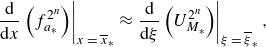 \begin{eqnarray} \left .\dfrac {{\textrm{d}}}{{\textrm{d}}x}\left (f^{2^{n}}_{a_*}\right )\right |_{x\,=\,\overline {x}_*}\approx \left .\dfrac {{\textrm{d}}}{{\textrm{d}}\xi }\left (U^{2^n}_{M_*}\right )\right |_{\xi \,=\,\overline {\xi }_*}, \end{eqnarray}
which tells that the multiplier of the $2^n$
orbit of the map
$2^n$
orbit of the map $f_a$
must be reasonably well approximated by that of the universal map
$f_a$
must be reasonably well approximated by that of the universal map $U_M$
. This result is actually not surprising because (5.2) indicates that the dynamics induced by the map
$U_M$
. This result is actually not surprising because (5.2) indicates that the dynamics induced by the map $f^{2^n}_a(x)$
around
$f^{2^n}_a(x)$
around $x=X$
are quantitatively similar to those induced by
$x=X$
are quantitatively similar to those induced by $U_M^{2^n}(\xi )$
around
$U_M^{2^n}(\xi )$
around $\xi =0$
. The same argument can be made for the correspondence between solutions
$\xi =0$
. The same argument can be made for the correspondence between solutions $\overline {\xi }(M)$
and
$\overline {\xi }(M)$
and $\overline {x}(a)$
at any
$\overline {x}(a)$
at any $a=\mu M+a_\infty$
, which need no longer be a single point as the central branch cascade unfolds. For
$a=\mu M+a_\infty$
, which need no longer be a single point as the central branch cascade unfolds. For $a\in (a_*,a_{\infty })$
, stable periodic orbits in the two systems can be related in the same way, and the approximate equality of multipliers follows from (5.6) analogously. Moreover, the dynamical similarity is not limited to periodic orbits, but applies also to aperiodic solutions for
$a\in (a_*,a_{\infty })$
, stable periodic orbits in the two systems can be related in the same way, and the approximate equality of multipliers follows from (5.6) analogously. Moreover, the dynamical similarity is not limited to periodic orbits, but applies also to aperiodic solutions for $a\gt a_\infty$
. In general, we must interpret that the template solution
$a\gt a_\infty$
. In general, we must interpret that the template solution $\overline {\xi }=\overline {\xi }(M)$
consists of a set of points satisfying
$\overline {\xi }=\overline {\xi }(M)$
consists of a set of points satisfying $U_{M}^{2^n}(\xi _i)\in \overline {\xi }$
for all
$U_{M}^{2^n}(\xi _i)\in \overline {\xi }$
for all $\xi _i \in \overline {\xi }$
(i.e. the set is invariant under
$\xi _i \in \overline {\xi }$
(i.e. the set is invariant under $U_{M}^{2^n}$
). Then, (5.2) implies that the set
$U_{M}^{2^n}$
). Then, (5.2) implies that the set $\overline {x}(a)$
, defined as the collection of points
$\overline {x}(a)$
, defined as the collection of points $x_i=\gamma \xi _i+X$
for every
$x_i=\gamma \xi _i+X$
for every $\xi _i \in \overline {\xi }(M)$
, is invariant under
$\xi _i \in \overline {\xi }(M)$
, is invariant under $f_{a}^{2^n}$
. Chaotic solutions related by
$f_{a}^{2^n}$
. Chaotic solutions related by $a=\mu M+a_\infty$
will have approximately the same Lyapunov exponents due to (5.6). All in all, the similarity of central branch dynamics between the two systems extends naturally all the way up to the accumulation point and beyond.
$a=\mu M+a_\infty$
will have approximately the same Lyapunov exponents due to (5.6). All in all, the similarity of central branch dynamics between the two systems extends naturally all the way up to the accumulation point and beyond.
To find an adequate set of values for $\gamma , X, \mu ,$
and
$\gamma , X, \mu ,$
and $a_{\infty }$
, one must pick two points in one of the bifurcation diagrams and find their analogues in the other. As a proof of concept, we select the first and second period-doubling bifurcation points that are encountered upon increasing
$a_{\infty }$
, one must pick two points in one of the bifurcation diagrams and find their analogues in the other. As a proof of concept, we select the first and second period-doubling bifurcation points that are encountered upon increasing $M$
beyond
$M$
beyond $M_*$
, where we have the stable period-
$M_*$
, where we have the stable period- $2^n$
orbit, namely PD
$2^n$
orbit, namely PD $_{n+1}$
and PD
$_{n+1}$
and PD $_{n+2}$
. We call the values of the parameter and of the central branch state variable
$_{n+2}$
. We call the values of the parameter and of the central branch state variable $(M,\xi )=(M_{n+1},\hat {\xi }_{n+1})$
and
$(M,\xi )=(M_{n+1},\hat {\xi }_{n+1})$
and $(M_{n+2},\hat {\xi }_{n+2})$
for PD
$(M_{n+2},\hat {\xi }_{n+2})$
for PD $_{n+1}$
and PD
$_{n+1}$
and PD $_{n+2}$
, respectively (see figure 12
c). These same period-doubling bifurcation points are found to occur at
$_{n+2}$
, respectively (see figure 12
c). These same period-doubling bifurcation points are found to occur at $(a,x)=(a_{n+1},\hat {x}_{n+1})$
and
$(a,x)=(a_{n+1},\hat {x}_{n+1})$
and $(a_{n+2},\hat {x}_{n+2})$
for the dynamical system (5.1), which, in the context of our DNS computations, correspond to
$(a_{n+2},\hat {x}_{n+2})$
for the dynamical system (5.1), which, in the context of our DNS computations, correspond to $(R,\tau )=(R_{n+1},\hat {\tau }_{n+1})$
and
$(R,\tau )=(R_{n+1},\hat {\tau }_{n+1})$
and $(R_{n+2},\hat {\tau }_{n+2})$
of § 4. The matching of both points from one bifurcation diagram to the other is accomplished by enforcing
$(R_{n+2},\hat {\tau }_{n+2})$
of § 4. The matching of both points from one bifurcation diagram to the other is accomplished by enforcing $M_{m}= (a_{m}-a_{\infty })/\mu$
and
$M_{m}= (a_{m}-a_{\infty })/\mu$
and $\hat {\xi }_{m}=(\hat {x}_{m}-X)/\gamma$
for
$\hat {\xi }_{m}=(\hat {x}_{m}-X)/\gamma$
for $m=n+1$
and
$m=n+1$
and $n+2$
. Solving the four resulting algebraic equations, we get
$n+2$
. Solving the four resulting algebraic equations, we get
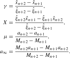 \begin{equation} \begin{array}{rcl} \gamma & = & \displaystyle {\frac {\hat {x}_{n+2}-\hat {x}_{n+1}}{\hat {\xi }_{n+2}-\hat {\xi }_{n+1}}},\\[1em] X & = & \displaystyle {\frac {\hat {\xi }_{n+2}\hat {x}_{n+1} -\hat {\xi }_{n+1} \hat {x}_{n+2}}{\hat {\xi }_{n+2}-\hat {\xi }_{n+1}}},\\[1em] \mu & = & \displaystyle {\frac {a_{n+2}-a_{n+1}}{M_{n+2}-M_{n+1}} }, \\[1em] a_{\infty } & = & \displaystyle {\frac {M_{n+2} a_{n+1} -M_{n+1}a_{n+2} }{M_{n+2}-M_{n+1}}}. \end{array} \end{equation}
If we set $n=2$
and exploit the DNS results of figure 10, the quadruplet of matching parameters takes the values
$n=2$
and exploit the DNS results of figure 10, the quadruplet of matching parameters takes the values $(\gamma , X,\mu , a_{\infty })\approx (-0.02518,0.2496,-0.4629,395.7213)$
. Finally, applying the transformation
$(\gamma , X,\mu , a_{\infty })\approx (-0.02518,0.2496,-0.4629,395.7213)$
. Finally, applying the transformation
 \begin{equation} \overline {x}(a)=\gamma \overline {\xi }(M)+X, \qquad a=\mu M+a_{\infty } \end{equation}
to the full cascade generated by system (5.5) results in the branch arrangement shown in figure 12(d). The transformed cascade exhibits a remarkably good agreement with DNS for the central branch (black dots). However, the quality of the match does not carry over to the rest of the template branches. It is precisely in this sense that the approximation (5.2) is to be considered only local.
The prediction can, however, be straightforwardly extended to all $2^n$
branches of the cascade undergone by the system (5.1), by simply allowing for a different set of scaling and translation parameters for each of the branches. The transformation of the
$2^n$
branches of the cascade undergone by the system (5.1), by simply allowing for a different set of scaling and translation parameters for each of the branches. The transformation of the $j$
th branch is performed according to
$j$
th branch is performed according to
 \begin{equation} x_j^J(a)=\gamma _j \xi _j^J(M)+X_j, \qquad a=\mu M+a_{\infty }, \qquad j=1,2,3,\dots ,J, \end{equation}
where the pairs $(\gamma _j,X_j)$
are obtained by matching the bifurcation points in the respective bifurcation diagrams, following the same procedure as for the central branch. The prediction thus obtained for the complete unfolding of the bifurcation cascade undergone by the DNS is shown in figure 13. The agreement is now excellent for all four cascade branches. The success of the branch-by-branch matching process follows from the fact that the map
$(\gamma _j,X_j)$
are obtained by matching the bifurcation points in the respective bifurcation diagrams, following the same procedure as for the central branch. The prediction thus obtained for the complete unfolding of the bifurcation cascade undergone by the DNS is shown in figure 13. The agreement is now excellent for all four cascade branches. The success of the branch-by-branch matching process follows from the fact that the map $f^{2^n}_a(x)$
has
$f^{2^n}_a(x)$
has $J=2^n$
extrema, the approximation (5.2) being applicable to each individually. Note that, in the chaotic regime after the accumulation point, the dynamics of the two systems is not expected to match in detail due to the sensitivity to initial conditions. Nonetheless, the statistical properties should, in principle, be in fair agreement, as evidenced by figure 13.
$J=2^n$
extrema, the approximation (5.2) being applicable to each individually. Note that, in the chaotic regime after the accumulation point, the dynamics of the two systems is not expected to match in detail due to the sensitivity to initial conditions. Nonetheless, the statistical properties should, in principle, be in fair agreement, as evidenced by figure 13.
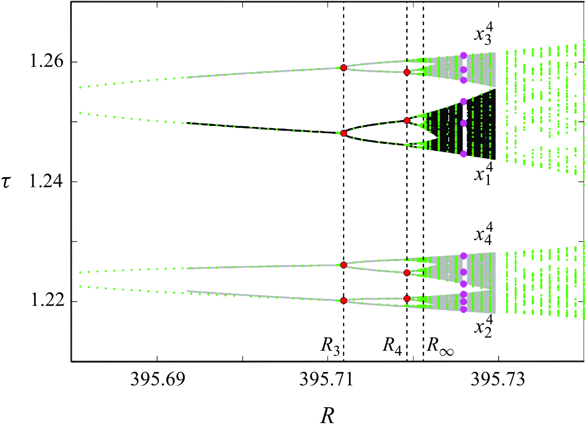
Figure 13. Branch-by-branch matching of period-doubling cascades. The black and grey points are the template branches shown in figure 12(b), re-adjusted according to the rescaling (5.9). The green points are the same DNS data as in figure 5(b). The matching process is based on the eight red points. The magenta points correspond to the P $_{12}$
orbit in the Taylor–Couette system.
$_{12}$
orbit in the Taylor–Couette system.
For simplicity, we have limited our comparison across systems to orbits of the same period. It is also possible to relate stable orbits of different periods, as Feigenbaum (Reference Feigenbaum1982) did, to demonstrate the self-similarity of the bifurcation diagram (see Appendix). Furthermore, our theoretical result is consistent with the fact that self-similarity also holds beyond the accumulation point, and that the Lyapunov exponent exhibits the scaling law observed by Huberman & Rudnick (Reference Huberman and Rudnick1980). However, a detailed comparison of statistical quantities such as Lyapunov exponents is beyond the scope of our analysis, given that statistical convergence requires unaffordably long simulation times in the vicinity of the accumulation point (see Tirnakli, Tsallis & Beck Reference Tirnakli, Tsallis and Beck2009, for example). Instead, to gauge the accuracy of the prediction beyond the accumulation point, we have run DNS at a value of $R$
for which the occurrence of a periodic window with a P
$R$
for which the occurrence of a periodic window with a P $_{12}$
orbit is anticipated. The time series of the Taylor–Couette system indeed appears to converge to a stable periodic orbit, which we have confirmed to be the Navier–Stokes counterpart of P
$_{12}$
orbit is anticipated. The time series of the Taylor–Couette system indeed appears to converge to a stable periodic orbit, which we have confirmed to be the Navier–Stokes counterpart of P $_{12}$
employing the PNK method (magenta dots in figure 13).
$_{12}$
employing the PNK method (magenta dots in figure 13).
All self-similar features of the template period-doubling cascade should also show up in any cascade generated by a unimodal map. This implies that any other unimodal map, including the long-studied logistic map, could have been employed as a template. The advantage of the $U_M$
defined in (5.4) stems from its natural emergence in the derivation of the approximation theory (as seen in Appendix), which grants very rapid convergence to universal dynamics by construction. Extending the prediction method to more general cases is straightforward using the results by Briggs (Reference Briggs1991).
$U_M$
defined in (5.4) stems from its natural emergence in the derivation of the approximation theory (as seen in Appendix), which grants very rapid convergence to universal dynamics by construction. Extending the prediction method to more general cases is straightforward using the results by Briggs (Reference Briggs1991).
The core of our prediction method lies in completely separating the map-dependent scaling/translating parameters $(\mu , a_{\infty }, \gamma _j, X_j)$
from all universality-related considerations. A careful reading of Feigenbaum’s work suggests that he was likely aware of this possibility. Notably, the method of trajectory scaling functions was specifically designed to eliminate all ingredients that depend on any particular map. However, to the authors’ knowledge, there is no direct assertion in the literature pointing at the feasibility of such predictions, let alone their applicability beyond the accumulation point.
$(\mu , a_{\infty }, \gamma _j, X_j)$
from all universality-related considerations. A careful reading of Feigenbaum’s work suggests that he was likely aware of this possibility. Notably, the method of trajectory scaling functions was specifically designed to eliminate all ingredients that depend on any particular map. However, to the authors’ knowledge, there is no direct assertion in the literature pointing at the feasibility of such predictions, let alone their applicability beyond the accumulation point.
6. Conclusions
We have studied in detail a period-doubling cascade that arises in subcritical counter-rotating Taylor–Couette flow employing small computational domains of annular-parallelogram shape. The cascade is seeded from a family of drifting rotating waves discovered by W22 and eventually leads to a chaotic regime fuelled by the self-sustained process of wall-bounded shear flows. Although the Navier–Stokes equations should formally be considered an infinite-dimensional dynamical system, the dynamics is often confined to finite-dimensional manifolds in phase space, sometimes designated as inertial manifolds (Temam Reference Temam1989). This low dimensionality has recently attracted significant attention (Ding et al. Reference Ding, Chaté, Cvitanović, Siminos and Takeuchi2016; Haller et al. Reference Haller, Kaszás, Liu and Axås2023), as it affords valuable insight into the underlying dynamics of the flow, sometimes leading to simplified models whose numerical simulation is computationally more tractable. Our results can be interpreted as an extreme case of simplification that ultimately leads to a one-dimensional map representation.
A pivotal outcome of our analysis is the confirmation of Feigenbaum universality to an unprecedented degree of accuracy in the context of fluid dynamics. Our success is largely ascribable to the fast development of computational power over the past few decades, along with the outstanding numerical accuracy of the methods we employ to solve Navier–Stokes flows, which altogether has rendered thorough parameter sweeps feasible. That said, establishing universality has required very long and costly numerical simulations, a refined parametric exploration, and the deployment of very accurate numerical techniques for the detailed analysis of the asymptotic convergence of relative periodic orbits, the assessment of their stability and the computation of period-doubling bifurcation points. Determining both the first and second Feigenbaum constants to the third significant digit demands the precise computation of up to the seventh period-doubling bifurcation along the cascade. This has enabled an accurate estimation of the accumulation point and, with it, the unambiguous exposure of the self-similar structure of the period-doubling bifurcation cascade. A key element to make the analysis systematic has been the deployment of a convenient Poincaré section based on torque balance, which provides a robust sampling method to validate theories of unimodal discrete-time dynamical systems.
Furthermore, our results constitute the first confirmation of universality in a fluid flow problem subject to subcritical turbulent transition. A detailed study of period-doubling cascades is contingent on the existence and identification of a stable solution. In subcritical shear flows, stable solutions are rare and can only occasionally be found by working with minimal flow units and/or symmetry subspaces. We were fortunate enough to find one such solution in W22 that happens to be at the origin of a period-doubling cascade. It is also noteworthy that all solutions along the period doubling cascade exhibit spatial drift, a property that is unique to our system among the many previous studies on the subject (see table 1). As expected, the conventional Feigenbaum theory becomes applicable to the Taylor–Couette phase space once reduced by the method of slices (Budanur et al. Reference Budanur, Cvitanović, Davidchack and Siminos2015).
Drawing from Feigenbaum’s theory, we have further developed a method to predict the bifurcation diagram of the period-doubling cascade all the way up to the accumulation point and, remarkably, also beyond. This approach has broader applicability than the method of trajectory scaling functions (Feigenbaum Reference Feigenbaum1983; Belmonte et al. Reference Belmonte, Vinson, Glazier, Gunaratne and Kenny1988), which is limited to scrutinising stable orbits with the same value of the multiplier. Our prediction method is simple: it only requires stretching and shifting a template bifurcation diagram produced by any smooth unimodal map at hand. The scaling and translating parameters must be chosen such that the template bifurcation diagram aligns with the period-doubling cascade of the target system (in our case, Taylor–Couette flow). This can be accomplished, for example, by matching two bifurcation points across systems. The remainder of the transformed template diagram provides the prediction for the target system. The prediction results are useful, among other things, to anticipate the location of periodic windows in the bifurcation diagram of the target system beyond the accumulation point. The emergence of a stable orbit in the Taylor–Couette system precisely within the expected parameter range attests to the exceptional predictive capability of the method.
Our analysis further provides a theoretical explanation for the self-similarity that occurs in the reverse cascade following the accumulation point (see the Appendix). Since the theoretical result holds universally for unimodal maps, the excellent agreement between our DNS data and the reference one-dimensional map implies that self-similarity can be reasonably expected to extend beyond the accumulation point also for the Navier–Stokes system.
The observation of Feigenbaum universality in our Taylor–Couette set-up provides evidence that the dynamics around the accumulation point can indeed be approximated by a nearly one-dimensional discrete map when analysed on an appropriate Poincaré section. Our finding further provides a handy playground for testing the application of iconic theorems from the early days of chaos theory, such as Li–Yorke or Sharkovsky’s (Sharkovskii Reference Sharkovskii1964; Li & Yorke Reference Li and Yorke1975), as well as cycle expansion theory (Cvitanović et al. Reference Cvitanović, Rrutuso, Mainieri, Tanner and Vattay2016), to a fluid dynamics problem. It is our intention to explore the significance and implications of these theories to the field of fluid dynamics in the near future.
As briefly commented in § 1, understanding the laminar–turbulent pattern-formation aspects of subcritical transition using stochastic theories (Hof Reference Hof2023) requires the prior occurrence of chaotic dynamics in the system. In shear flows, the incipient chaotic dynamics is only transient, such that the underlying chaotic saddle is not accessible through experiments or DNS. The scenario we have dissected offers a possible mechanism for the formation of one such chaotic saddle because our period-doubling cascade (i) occurs globally in the full annulus and (ii) is unstable to subharmonic (spatially modulational) perturbations, as can be inferred from W22. Both the full and elongated domains of figure 1(b) are simultaneously compatible with spiral turbulence and with the period-doubling cascade we address here. Evidence for property (ii) can indeed be drawn from W22, where the subharmonic instability of DRW, along with all solutions bifurcated from it in our small domain, was shown to contribute decisively to the formation of the laminar–turbulent helical pattern that is characteristic of the spiral turbulence regime. Therefore, although other mechanisms have been shown to produce localised chaotic sets that may be held responsible for intermittency in some cases (see Paranjape et al. Reference Paranjape, Yalnız, Duguet, Budanur and Hof2023 for an example in channel flow), also a period-doubling cascade might work concurrently with a modulational instability to the same effect.
Funding
This research is supported by the Australian Research Council Discovery Project DP230102188 and the Ministerio de Ciencia, Innovación y Universidades (Agencia Estatal de Investigación, project nos. PID 2020–114043 GB-I00 (MCIN/AEI/10.13039/501100011033) and PID 2023–150029NB-I00 (MCIN/AEI/10.13039/501100011033/FEDER, UE). B.W.’s and R.A.’s research has been funded by the European Union’s Horizon 2020 research and innovation programme (Marie Skłodowska-Curie Grant Agreement No. 101034413). R.A. has also been funded by the Austrian Science Fund (FWF) 10.55776/ESP1481224.
Declaration of interests
The authors report no conflict of interest.
Appendix. Derivation of a universal approximation to a unimodal map and the conditions for validity
Consider the one-dimensional map (5.1), with $f_a(x)$
a unimodal function, undergoing a period-doubling cascade as the parameter
$f_a(x)$
a unimodal function, undergoing a period-doubling cascade as the parameter $a$
is increased. The location where the function has a maximum for
$a$
is increased. The location where the function has a maximum for $a=a_\infty$
, the accumulation point, is denoted as
$a=a_\infty$
, the accumulation point, is denoted as $X=\text {argmax} f_{a_\infty }(x)$
. It will be convenient to shift the coordinate according to
$X=\text {argmax} f_{a_\infty }(x)$
. It will be convenient to shift the coordinate according to $y=x-X$
and define the shifted map as
$y=x-X$
and define the shifted map as $F_{a}(y)=f_{a}(y+X)-X$
.
$F_{a}(y)=f_{a}(y+X)-X$
.
If $a$
is close to the accumulation point
$a$
is close to the accumulation point $a_{\infty }$
, the function
$a_{\infty }$
, the function $F_{a}$
may be approximated by a Taylor expansion truncated at first order, i.e.
$F_{a}$
may be approximated by a Taylor expansion truncated at first order, i.e.
 \begin{eqnarray} F_{a}(y) \approx \varPsi (y)+(a-a_{\infty })\psi (y), \end{eqnarray}
where $\varPsi =F_a |_{a=a_{\infty }}$
and
$\varPsi =F_a |_{a=a_{\infty }}$
and $\psi =\left . \partial _a F_{a}\right |_{a=a_{\infty }}$
. Unimodal maps are known to be infinitely renormalisable at accumulation points (see Lanford III Reference Lanford III1982, for example). Therefore, for large
$\psi =\left . \partial _a F_{a}\right |_{a=a_{\infty }}$
. Unimodal maps are known to be infinitely renormalisable at accumulation points (see Lanford III Reference Lanford III1982, for example). Therefore, for large $n$
and
$n$
and $a=a_\infty$
, one must be able to find a function
$a=a_\infty$
, one must be able to find a function $g$
, satisfying
$g$
, satisfying $\mathcal {R}[g]=g$
, such that
$\mathcal {R}[g]=g$
, such that
 \begin{eqnarray} \mathcal {R}^n[\varPsi ](y)\approx g(y). \end{eqnarray}
Note that $\gamma =g(0)$
is not necessarily unity and depends on the map
$\gamma =g(0)$
is not necessarily unity and depends on the map $f_a$
. The function
$f_a$
. The function $g$
and the Feigenbaum function
$g$
and the Feigenbaum function $G$
introduced in § 1 are related by
$G$
introduced in § 1 are related by
 \begin{eqnarray} G(\xi )=g(\gamma \xi )/\gamma . \end{eqnarray}
Next, we consider the Fréchet derivative of $\mathcal {R}$
, in the direction of function
$\mathcal {R}$
, in the direction of function $h(y)$
, and evaluated at function
$h(y)$
, and evaluated at function $f(y)$
:
$f(y)$
:
 \begin{align} \mathcal {L}_{f}[h](y) = \lim _{\epsilon \rightarrow 0} \frac {\mathcal {R}[f+\epsilon h](y)-\mathcal {R}[f](y)}{\epsilon } = \alpha h\left (f \left (\frac {y}{\alpha }\right )\right )+\alpha f' \left (f \left (\frac {y}{\alpha } \right ) \right ) h\left (\frac {y}{\alpha } \right ). \end{align}
The operative expression of $\mathcal {L}_{f}[h](y)$
in terms of
$\mathcal {L}_{f}[h](y)$
in terms of $f$
and
$f$
and $h$
is a well-known result (see Briggs Reference Briggs1991; Thurlby Reference Thurlby2021, for example). The definition (A4), combined with the expansion (A1), implies
$h$
is a well-known result (see Briggs Reference Briggs1991; Thurlby Reference Thurlby2021, for example). The definition (A4), combined with the expansion (A1), implies $\mathcal {L}_{\varPsi }[\psi ] \approx (\mathcal {R}[F_{a}]-\mathcal {R}[\varPsi ])/(a-a_{\infty })$
, such that simple algebraic manipulation yields
$\mathcal {L}_{\varPsi }[\psi ] \approx (\mathcal {R}[F_{a}]-\mathcal {R}[\varPsi ])/(a-a_{\infty })$
, such that simple algebraic manipulation yields
 \begin{eqnarray} \mathcal {R}[F_{a}]\approx \mathcal {R}[\varPsi ]+(a-a_{\infty })\mathcal {L}_{\varPsi }[\psi ]. \end{eqnarray}
Moreover, it can be shown by induction that the $n$
th renormalisation of
$n$
th renormalisation of $F_a$
is given by
$F_a$
is given by
 \begin{eqnarray} \mathcal {R}^n[F_{a}]\approx \mathcal {R}^n[\varPsi ]+(a-a_{\infty })\mathcal {J}_{n}[\psi ], \end{eqnarray}
where $\mathcal {J}_{n}=\mathcal {L}_{\mathcal {R}^{n-1}[\varPsi ]}\circ \mathcal {L}_{\mathcal {R}^{n-2}[\varPsi ]} \circ \dots \circ \mathcal {L}_{\mathcal {R}^0[\varPsi ]}$
and, of course,
$\mathcal {J}_{n}=\mathcal {L}_{\mathcal {R}^{n-1}[\varPsi ]}\circ \mathcal {L}_{\mathcal {R}^{n-2}[\varPsi ]} \circ \dots \circ \mathcal {L}_{\mathcal {R}^0[\varPsi ]}$
and, of course, $\mathcal {R}^0[\varPsi ]=\varPsi$
. To deduce (A6), let us define
$\mathcal {R}^0[\varPsi ]=\varPsi$
. To deduce (A6), let us define $Q_k = \mathcal {R}^k[\varPsi ]+(a-a_{\infty })\mathcal {J}_{k}[\psi ]$
. For
$Q_k = \mathcal {R}^k[\varPsi ]+(a-a_{\infty })\mathcal {J}_{k}[\psi ]$
. For $n=1$
, the statement (A6) reduces to
$n=1$
, the statement (A6) reduces to $\mathcal {R}[F_{a}] \approx Q_1$
, which is trivially satisfied in view of (A5). Now, assuming that
$\mathcal {R}[F_{a}] \approx Q_1$
, which is trivially satisfied in view of (A5). Now, assuming that $\mathcal {R}^k[F_a]\approx Q_k$
holds at step
$\mathcal {R}^k[F_a]\approx Q_k$
holds at step $k$
, we just need to prove that
$k$
, we just need to prove that $\mathcal {R}^{k+1}[F_a]\approx Q_{k+1}$
also holds. Using (A4), we get
$\mathcal {R}^{k+1}[F_a]\approx Q_{k+1}$
also holds. Using (A4), we get
 \begin{eqnarray} \mathcal {J}_{k+1}[\psi ] = \mathcal {L}_{\mathcal {R}^{k}[\varPsi ]}\left [\mathcal {J}_{k}[\psi ]\right ] \approx \frac {\mathcal {R}\left [\mathcal {R}^{k}[\varPsi ]+(a-a_{\infty })\mathcal {J}_{k}[\psi ]\right ]-\mathcal {R}\left [\mathcal {R}^{k} [\varPsi ]\right ]}{a-a_{\infty }}, \end{eqnarray}
which implies $\mathcal {R}[Q_{k}] \approx \mathcal {R}^{k+1}[\varPsi ]+(a-a_{\infty })\mathcal {J}_{k+1}[\psi ] = Q_{k+1}$
. Operating
$\mathcal {R}[Q_{k}] \approx \mathcal {R}^{k+1}[\varPsi ]+(a-a_{\infty })\mathcal {J}_{k+1}[\psi ] = Q_{k+1}$
. Operating $\mathcal {R}$
on the induction step assumption yields
$\mathcal {R}$
on the induction step assumption yields $\mathcal {R}^{k+1}[F_a]\approx \mathcal {R}[Q_k] \approx Q_{k+1}$
, which completes the proof of (A6).
$\mathcal {R}^{k+1}[F_a]\approx \mathcal {R}[Q_k] \approx Q_{k+1}$
, which completes the proof of (A6).
The leading eigenvalue of the eigenvalue problem $\mathcal {L}_g[\varphi ]=\delta \varphi$
is
$\mathcal {L}_g[\varphi ]=\delta \varphi$
is $\delta$
(i.e. Feigenbaum’s first constant) with associated eigenfunction
$\delta$
(i.e. Feigenbaum’s first constant) with associated eigenfunction $\varphi$
. For sufficiently large
$\varphi$
. For sufficiently large $n$
, the relation
$n$
, the relation
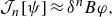 \begin{eqnarray} \mathcal {J}_{n}[\psi ] \approx \delta ^n B \varphi , \end{eqnarray}
with $B$
some constant, is expected to hold, because
$B$
some constant, is expected to hold, because $\mathcal {J}_{n}$
results from the repeated application, many times, of
$\mathcal {J}_{n}$
results from the repeated application, many times, of $\mathcal {L}_g$
, which amplifies the most unstable mode. The eigenvalue problem can be recast in terms of the universal functions as
$\mathcal {L}_g$
, which amplifies the most unstable mode. The eigenvalue problem can be recast in terms of the universal functions as $\mathcal {L}_G[\varPhi ]=\delta \varPhi$
, where
$\mathcal {L}_G[\varPhi ]=\delta \varPhi$
, where
 \begin{eqnarray} \varPhi (\xi )=\mu B\varphi (\gamma \xi )/\gamma \end{eqnarray}
is normalised to $\varPhi (0)=1$
choosing the scaling factor appropriately as
$\varPhi (0)=1$
choosing the scaling factor appropriately as $\mu =\gamma /B\varphi (0)$
.
$\mu =\gamma /B\varphi (0)$
.
Substituting (A2) and (A8) in (A6) yields
 \begin{eqnarray} \mathcal {R}^n[F_{a}](y)\approx g(y)+(a-a_{\infty })\delta ^nB\varphi (y). \end{eqnarray}
Further replacing $g$
and
$g$
and $\phi$
using (A3) and (A9), respectively, we obtain
$\phi$
using (A3) and (A9), respectively, we obtain
 \begin{eqnarray} \mathcal {R}^n[F_a](y)=\alpha ^n F^{2^n}_{a}\left (\frac {y}{\alpha ^n} \right )\approx \gamma \left \{G\left (\frac {y}{\gamma } \right ) + \delta ^n (a-a_{\infty })\mu ^{-1}\varPhi \left (\frac {y}{\gamma } \right ) \right \}, \end{eqnarray}
where we have made explicit the effect of the renormalisation operator upon repeated application. To get back to the original map, we can use in (A11) the easily verifiable proposition that repeated application of the original and shifted maps is related by $F_{a}^n(y)=f_{a}^n(y+X)-X$
for any
$F_{a}^n(y)=f_{a}^n(y+X)-X$
for any $n\in \mathbb {N}$
. Combined with the definition of the universal function (5.4), the approximation
$n\in \mathbb {N}$
. Combined with the definition of the universal function (5.4), the approximation
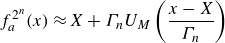 \begin{eqnarray} f^{2^n}_{a}(x) \approx X+\Gamma _n U_M\left (\frac {x-X}{\Gamma _n} \right ) \end{eqnarray}
follows directly, where the rescaled parameter $M$
and magnification rate of the variable
$M$
and magnification rate of the variable $\Gamma _n$
have been defined as
$\Gamma _n$
have been defined as
 \begin{eqnarray} M=\delta ^n \mu ^{-1} (a-a_{\infty })\;\;\text {and}\;\; \Gamma _n=\gamma /\alpha ^n. \end{eqnarray}
Let us now consider what conditions are necessary for the approximation (A12) to be valid, besides the one requiring that $2^n$
must be large. The reliability of (A12) depends on the degree of trust one can place on the approximations (A2) and (A8). It is important to note that, in renormalisation theory, comparisons of functions are conducted on magnified scales. That is, while (A2) may be a good approximation on the scale where
$2^n$
must be large. The reliability of (A12) depends on the degree of trust one can place on the approximations (A2) and (A8). It is important to note that, in renormalisation theory, comparisons of functions are conducted on magnified scales. That is, while (A2) may be a good approximation on the scale where $y/\alpha ^n=(x-X)/\alpha ^n$
is not too large, it may not hold true on the original scale where
$y/\alpha ^n=(x-X)/\alpha ^n$
is not too large, it may not hold true on the original scale where $y\sim O(1)$
(mathematically, this can be easily understood by considering the case where
$y\sim O(1)$
(mathematically, this can be easily understood by considering the case where $\varPsi$
is topologically conjugate to
$\varPsi$
is topologically conjugate to $g$
). In (A12), it suffices to consider
$g$
). In (A12), it suffices to consider $U_M(\xi )$
with the argument in the range
$U_M(\xi )$
with the argument in the range $\xi \in [-1,1]$
, which encompasses the entire period-doubling cascade of (5.5). Hence, the restriction
$\xi \in [-1,1]$
, which encompasses the entire period-doubling cascade of (5.5). Hence, the restriction $|(x-X)/\Gamma _n| \lt 1$
, which makes (A2) only locally valid. The approximation (A8) is, again, local. Moreover, to use the approximation (A7) at level
$|(x-X)/\Gamma _n| \lt 1$
, which makes (A2) only locally valid. The approximation (A8) is, again, local. Moreover, to use the approximation (A7) at level $k=n$
,
$k=n$
, $|\delta ^n(a-a_{\infty })|$
must necessarily be small, so we require
$|\delta ^n(a-a_{\infty })|$
must necessarily be small, so we require $|\delta ^n M|\ll 1$
.
$|\delta ^n M|\ll 1$
.
The approximation (A12) must also hold for $U_M(\xi )$
itself, as it is unimodal in the range
$U_M(\xi )$
itself, as it is unimodal in the range $\xi \in [-1,1]$
. We can therefore set
$\xi \in [-1,1]$
. We can therefore set $n=m$
,
$n=m$
, $x=\tilde {x}$
,
$x=\tilde {x}$
, $a=\tilde {M}$
,
$a=\tilde {M}$
, $X=0$
,
$X=0$
, $a_{\infty }=0$
,
$a_{\infty }=0$
, $\mu =\tilde {\mu }$
,
$\mu =\tilde {\mu }$
, $\gamma =\tilde {\gamma }$
and
$\gamma =\tilde {\gamma }$
and $f_a=U_{\tilde {M}}$
in (A12)–(A13) to obtain
$f_a=U_{\tilde {M}}$
in (A12)–(A13) to obtain
 \begin{eqnarray} U^{2^m}_{\tilde {M}}(\tilde {x}) \approx \tilde {\Gamma }_m U_M\left (\frac {\tilde {x}}{\tilde {\Gamma }_m} \right ),\qquad M= \delta ^m \tilde {M}/\tilde {\mu },\qquad \tilde {\Gamma }_m=\tilde {\gamma }/\alpha ^m, \end{eqnarray}
which should work as long as $2^m$
is large,
$2^m$
is large, $|\tilde {x}/\tilde {\Gamma }_m|\lt 1$
and
$|\tilde {x}/\tilde {\Gamma }_m|\lt 1$
and $|\delta ^m \tilde {M}|\ll 1$
.
$|\delta ^m \tilde {M}|\ll 1$
.
Finally, particularising (A12) for $n=\ell +m$
, we get
$n=\ell +m$
, we get
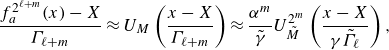 \begin{eqnarray} \frac {f^{2^{\ell +m}}_{a}(x)-X}{\Gamma _{\ell +m}} \approx U_{M} \left ( \frac {x-X}{\Gamma _{\ell +m}} \right )\approx \frac {\alpha ^m}{\tilde {\gamma }}U_{\tilde {M}}^{2^m}\left (\frac {x-X}{\gamma \tilde {\Gamma }_{\ell }} \right ), \end{eqnarray}
where the rightmost approximation is found by setting $\tilde {x}=(\tilde {\gamma }/\gamma )(x-X)\alpha ^{-\ell }$
in (A14). The parameters
$\tilde {x}=(\tilde {\gamma }/\gamma )(x-X)\alpha ^{-\ell }$
in (A14). The parameters $a$
and
$a$
and $\tilde {M}$
are linked by
$\tilde {M}$
are linked by $\tilde {M}=\tilde {\mu }\delta ^{-m}M=(\tilde {\mu }/\mu )\delta ^{\ell }(a-a_{\infty })$
. We can simplify the notation by renaming (
$\tilde {M}=\tilde {\mu }\delta ^{-m}M=(\tilde {\mu }/\mu )\delta ^{\ell }(a-a_{\infty })$
. We can simplify the notation by renaming ( $\gamma /\tilde {\gamma }$
) and (
$\gamma /\tilde {\gamma }$
) and ( $\mu /\tilde {\mu }$
) as
$\mu /\tilde {\mu }$
) as $\gamma$
and
$\gamma$
and $\mu$
, respectively. In summary, the approximation
$\mu$
, respectively. In summary, the approximation
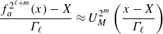 \begin{eqnarray} \frac {f^{2^{\ell +m}}_{a}(x)-X}{\Gamma _{\ell }} \approx U_{M}^{2^m} \left ( \frac {x-X}{\Gamma _{\ell }} \right ) \end{eqnarray}
is obtained if we redefine
 \begin{eqnarray} M = \delta ^{\ell }\mu ^{-1}(a-a_{\infty }), \qquad \Gamma _\ell =\gamma /\alpha ^\ell . \end{eqnarray}
This approximation is valid for $2^m$
large, irrespective of the value of
$2^m$
large, irrespective of the value of $\ell =0,1,2\dots$
, as long as
$\ell =0,1,2\dots$
, as long as
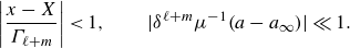 \begin{eqnarray} \left |\frac {x-X}{\Gamma _{\ell +m}} \right | \lt 1,\qquad |\delta ^{\ell +m}\mu ^{-1} (a-a_{\infty })|\ll 1. \end{eqnarray}
The approximation (5.2) and conditions (5.3) quoted in the main text correspond to the case $\ell =0$
.
$\ell =0$
.
The self-similarity of the period-doubling cascade follows from the validity of the approximation (A16). Suppose we detect a period- $2^m$
stable orbit in (5.5) for
$2^m$
stable orbit in (5.5) for $M$
negative but close to zero. Then, the relation (A16) asserts the presence of period-
$M$
negative but close to zero. Then, the relation (A16) asserts the presence of period- $2^{\ell +m}$
orbits in (5.1) at
$2^{\ell +m}$
orbits in (5.1) at $a=a_\ell =\delta ^{-\ell }\mu M+a_{\infty }$
for every
$a=a_\ell =\delta ^{-\ell }\mu M+a_{\infty }$
for every $\ell \in \mathbb {N}$
. Moreover, the orbits must share the same multiplier, because an argument analogous to (5.6) can be applied.
$\ell \in \mathbb {N}$
. Moreover, the orbits must share the same multiplier, because an argument analogous to (5.6) can be applied.
The same self-similarity theory applies also to values of the parameter beyond the accumulation point. For instance, suppose we fix $M$
at a small positive number so that a period
$M$
at a small positive number so that a period $2^m p$
window is observed in (5.5), with
$2^m p$
window is observed in (5.5), with $p$
an odd number. Then, we can expect a period
$p$
an odd number. Then, we can expect a period $2^{\ell +m} p$
window in (5.1) at
$2^{\ell +m} p$
window in (5.1) at $a_\ell = \delta ^{-\ell }\mu M+a_{\infty }$
for every
$a_\ell = \delta ^{-\ell }\mu M+a_{\infty }$
for every $\ell \in \mathbb {N}$
. Even if the dynamics are predominantly chaotic, we can still expect similarity of the dynamics in the statistical sense. In particular, if
$\ell \in \mathbb {N}$
. Even if the dynamics are predominantly chaotic, we can still expect similarity of the dynamics in the statistical sense. In particular, if $\lambda (M_*)$
is the Lyapunov exponent of (5.5) at
$\lambda (M_*)$
is the Lyapunov exponent of (5.5) at $M=M_*$
, the Lyapunov exponent of (5.1) at
$M=M_*$
, the Lyapunov exponent of (5.1) at $a_\ell =\delta ^{-\ell }\mu M_*+a_{\infty }$
should approximately be
$a_\ell =\delta ^{-\ell }\mu M_*+a_{\infty }$
should approximately be $2^{-\ell }\lambda (M_*)$
. This is consistent with the observation by Huberman & Rudnick (Reference Huberman and Rudnick1980). Note that this implies that for all unimodal maps, the distribution of Lyapunov exponents is identical immediately past the accumulation point.
$2^{-\ell }\lambda (M_*)$
. This is consistent with the observation by Huberman & Rudnick (Reference Huberman and Rudnick1980). Note that this implies that for all unimodal maps, the distribution of Lyapunov exponents is identical immediately past the accumulation point.


 Open access