


1. Introduction
In the following, we assess the magnetohydrodynamic (MHD) equilibrium and stability properties of the Infinity Two fusion pilot plant (FPP) baseline plasma physics design. Infinity Two is a four-field period, aspect ratio $A = 10$
, quasi-isodynamic (QI) configuration with optimised confinement at elevated density and high magnetic field (
$A = 10$
, quasi-isodynamic (QI) configuration with optimised confinement at elevated density and high magnetic field ( $B = 9\,$
T) (Hegna et al. Reference Hegna2025). An explicit goal of the optimisation was to demand robust magnetic surface integrity by avoiding low-order rational surfaces in the confinement region. For a configuration with a number of field periods (NFPs), this implies avoiding values of
$B = 9\,$
T) (Hegna et al. Reference Hegna2025). An explicit goal of the optimisation was to demand robust magnetic surface integrity by avoiding low-order rational surfaces in the confinement region. For a configuration with a number of field periods (NFPs), this implies avoiding values of ${\iota\kern-3.5pt\def\negativespace{}\mbox{-}\kern0.5pt}= ({\textrm{NFP}}/{M}),({2\times \textrm{NFP}}/{M}),({3\times \textrm{NFP}}/{M})$
, where
${\iota\kern-3.5pt\def\negativespace{}\mbox{-}\kern0.5pt}= ({\textrm{NFP}}/{M}),({2\times \textrm{NFP}}/{M}),({3\times \textrm{NFP}}/{M})$
, where $M$
is a small integer, typically of the order of
$M$
is a small integer, typically of the order of $1{-}2\times \textrm{NFP}$
. Additionally, the high-field approach used in the generation of Infinity Two allows for the desired deuterium–tritium (DT) FPP operation at relatively small
$1{-}2\times \textrm{NFP}$
. Additionally, the high-field approach used in the generation of Infinity Two allows for the desired deuterium–tritium (DT) FPP operation at relatively small $\beta$
, which relaxes the constraints imposed by ideal MHD stability considerations. Here,
$\beta$
, which relaxes the constraints imposed by ideal MHD stability considerations. Here, $\beta$
is the ratio of the volume averages of the plasma pressure and the magnetic pressure in the plasma:
$\beta$
is the ratio of the volume averages of the plasma pressure and the magnetic pressure in the plasma:
 \begin{align} \beta &= \frac {2\mu _0\langle p\rangle }{\langle B^2\rangle }, \end{align}
where $\langle \mathcal {L}\rangle$
indicates a volume average of the quantity
$\langle \mathcal {L}\rangle$
indicates a volume average of the quantity $\mathcal {L}$
. A related quantity of interest is
$\mathcal {L}$
. A related quantity of interest is $\beta _0\equiv 2 \mu _0 p_0 / \langle B^2\rangle$
, where
$\beta _0\equiv 2 \mu _0 p_0 / \langle B^2\rangle$
, where $p_0$
is the plasma pressure at the magnetic axis.
$p_0$
is the plasma pressure at the magnetic axis.
1.1. Magnetohydrodynamic equilibrium
The MHD equilibrium and stability properties of the plasma in a stellarator fusion pilot plant must be robust and predictable. The coils of a stellarator create a three-dimensional (3-D) magnetic field topology of closed, nested toroidal flux surfaces without the need of any plasma currents. This is not a trivial task, but techniques using the concept of a winding surface (Merkel Reference Merkel1987; Landreman Reference Landreman2017) and discrete space curves (Zhu et al. Reference Zhu, Hudson, Song and Wan2018) assist with the design of filamentary coils. These filamentary coils can be further optimised to maximise the volume of nested flux surfaces (Hanson & Cary Reference Hanson and Cary1984; Cary & Hanson Reference Cary and Hanson1986; Reiman et al. Reference Reiman2007; Smiet et al. Reference Smiet, Loizu, Balkovic and Baillod2025). On any of the flux surfaces, the trajectory of the magnetic field line can be traced to evaluate the rotational transform, ${\iota\kern-3.5pt\def\negativespace{}\mbox{-}\kern0.5pt}$
, defined as (Kruskal & Kulsrud Reference Kruskal and Kulsrud1958)
${\iota\kern-3.5pt\def\negativespace{}\mbox{-}\kern0.5pt}$
, defined as (Kruskal & Kulsrud Reference Kruskal and Kulsrud1958)
 \begin{equation} {\iota\kern-3.5pt\def\negativespace{}\mbox{-}\kern0.5pt} = \lim _{\Delta \phi \to \infty } \frac {\Delta \theta }{\Delta \phi }. \end{equation}
The poloidal ( $\theta$
) and toroidal (
$\theta$
) and toroidal ( $\phi$
) angle are associated with the short and long way around the torus, respectively. When surfaces with values of
$\phi$
) angle are associated with the short and long way around the torus, respectively. When surfaces with values of ${\iota\kern-3.5pt\def\negativespace{}\mbox{-}\kern0.5pt}$
close to low-order rationals are present within the plasma, there is a possibility that a resonant
${\iota\kern-3.5pt\def\negativespace{}\mbox{-}\kern0.5pt}$
close to low-order rationals are present within the plasma, there is a possibility that a resonant ${\iota\kern-3.5pt\def\negativespace{}\mbox{-}\kern0.5pt}\approx n/m$
island can open under certain conditions. The field lines wrap around and connect to opposite sides of the island. Fast parallel transport along the field lines provides an additional channel for the effective radial diffusion of energy and particles across the island. Experiments on W2-A (Grieger et al. Reference Grieger, Ohlendorf, Pacher, Wobig and Wolf1971) and W7-A (Cattanei, Dorst & Elsner Reference Cattanei1985) both demonstrated the importance of avoiding resonant values of
${\iota\kern-3.5pt\def\negativespace{}\mbox{-}\kern0.5pt}\approx n/m$
island can open under certain conditions. The field lines wrap around and connect to opposite sides of the island. Fast parallel transport along the field lines provides an additional channel for the effective radial diffusion of energy and particles across the island. Experiments on W2-A (Grieger et al. Reference Grieger, Ohlendorf, Pacher, Wobig and Wolf1971) and W7-A (Cattanei, Dorst & Elsner Reference Cattanei1985) both demonstrated the importance of avoiding resonant values of ${\iota\kern-3.5pt\def\negativespace{}\mbox{-}\kern0.5pt}$
in the plasma core. The maximum stored energy that could be maintained in the plasma was severely restricted when low-order rational surfaces were present. The derivative of the transform with respect to the minor radius
${\iota\kern-3.5pt\def\negativespace{}\mbox{-}\kern0.5pt}$
in the plasma core. The maximum stored energy that could be maintained in the plasma was severely restricted when low-order rational surfaces were present. The derivative of the transform with respect to the minor radius $\rho$
of the plasma is called the shear,
$\rho$
of the plasma is called the shear, $\textrm{d}{\iota\kern-3.5pt\def\negativespace{}\mbox{-}\kern0.5pt}/\textrm{d}\rho$
. Low-shear stellarators have windows of good operation when low-order rational values of
$\textrm{d}{\iota\kern-3.5pt\def\negativespace{}\mbox{-}\kern0.5pt}/\textrm{d}\rho$
. Low-shear stellarators have windows of good operation when low-order rational values of ${\iota\kern-3.5pt\def\negativespace{}\mbox{-}\kern0.5pt}$
can be avoided in the core region. Based on consideration of the Farey tree (Meiss Reference Meiss1992), large windows are adjacent to low-order rationals. However, the requirement of an edge resonance enables the use of island divertor solutions (Feng et al. Reference Feng, Kobayashi, Lunt and Reiter2011; Helander et al. Reference Helander2012). The divertor design and operation relies on the details of the resonant edge island or island remnants (Renner et al. Reference Renner, Boscary, Erckmann, Greuner, Grote, Sapper, Speth, Wesner and Wanner2000; Grigull et al. Reference Grigull2001; Morisaki et al. Reference Morisaki2005; Feng et al. Reference Feng, Kobayashi, Lunt and Reiter2011, Reference Feng2021).
${\iota\kern-3.5pt\def\negativespace{}\mbox{-}\kern0.5pt}$
can be avoided in the core region. Based on consideration of the Farey tree (Meiss Reference Meiss1992), large windows are adjacent to low-order rationals. However, the requirement of an edge resonance enables the use of island divertor solutions (Feng et al. Reference Feng, Kobayashi, Lunt and Reiter2011; Helander et al. Reference Helander2012). The divertor design and operation relies on the details of the resonant edge island or island remnants (Renner et al. Reference Renner, Boscary, Erckmann, Greuner, Grote, Sapper, Speth, Wesner and Wanner2000; Grigull et al. Reference Grigull2001; Morisaki et al. Reference Morisaki2005; Feng et al. Reference Feng, Kobayashi, Lunt and Reiter2011, Reference Feng2021).
1.2. MHD equilibrium limits and edge topology
Plasma-induced currents can change the field topology and location of the plasma and its edge. The plasma pressure in a stellarator generates a diamagnetic current. The variations of $1/|B^2|$
on a flux surface, combined with the divergence-free condition for the current density on that surface,
$1/|B^2|$
on a flux surface, combined with the divergence-free condition for the current density on that surface, $\nabla \cdot \vec{J}=0$
, requires the existence of a dipole-like current density, commonly referred to as the Pfirsch–Schlüter current (Pfirsch & Schlüte Reference Pfirsch and Schlüter1962). This current generates a dipole magnetic field that applies a net radial force on the plasma column. The resulting radial shift of the plasma column, called the Shafranov shift (Shafranov Reference Shafranov1963, Freidberg Reference Freidberg2014), sets an equilibrium limit if left uncompensated (Helander et al. Reference Helander2012; Freidberg Reference Freidberg2014). The neoclassical bootstrap current will alter the rotational transform and location of island structures. It also serves as a source of free energy for instabilities. For an island to serve as part of a detailed divertor design, it is essential to have good predictions regarding the edge topology at vacuum conditions, the operating point and points in between. Any sensitivities to plasma profiles and configuration details must be well understood and anticipated.
$\nabla \cdot \vec{J}=0$
, requires the existence of a dipole-like current density, commonly referred to as the Pfirsch–Schlüter current (Pfirsch & Schlüte Reference Pfirsch and Schlüter1962). This current generates a dipole magnetic field that applies a net radial force on the plasma column. The resulting radial shift of the plasma column, called the Shafranov shift (Shafranov Reference Shafranov1963, Freidberg Reference Freidberg2014), sets an equilibrium limit if left uncompensated (Helander et al. Reference Helander2012; Freidberg Reference Freidberg2014). The neoclassical bootstrap current will alter the rotational transform and location of island structures. It also serves as a source of free energy for instabilities. For an island to serve as part of a detailed divertor design, it is essential to have good predictions regarding the edge topology at vacuum conditions, the operating point and points in between. Any sensitivities to plasma profiles and configuration details must be well understood and anticipated.
1.3. MHD stability limits in stellarators
Three-dimensional fields can be beneficial for MHD stability, when applied correctly. The Compact Toroidal Hybrid (CTH) and W7-A both demonstrated that adding a small amount of vacuum transform with helical fields to net current-carrying toroidal plasmas provided a stabilising force that would suppress vertical instabilities (ArchMiller et al. Reference ArchMiller2014) and provide passive disruption avoidance (Team 1980; Pandya et al. Reference Pandya2015). CTH also showed that a fractional vacuum transform of only 10 % ( ${\iota\kern-3.5pt\def\negativespace{}\mbox{-}\kern0.5pt}_{\textrm{vac}} \geqslant 0.07$
) was sufficient to operate above the Greenwald density limit typical of tokamaks (Hartwell et al. Reference Hartwell2013).
${\iota\kern-3.5pt\def\negativespace{}\mbox{-}\kern0.5pt}_{\textrm{vac}} \geqslant 0.07$
) was sufficient to operate above the Greenwald density limit typical of tokamaks (Hartwell et al. Reference Hartwell2013).
Equilibrium effects such as pressure-induced changes in the plasma shape and location, and MHD stability limits can both restrict the level of $\beta$
that can be achieved. Under stable conditions, the maximum achievable limit of
$\beta$
that can be achieved. Under stable conditions, the maximum achievable limit of $\beta$
is set by the available heating power and the transport properties of the configuration. The exact details vary with the configuration. In most stellarators, crossing pressure-induced MHD stability boundaries tends to lead to soft-limits on the maximum sustainable
$\beta$
is set by the available heating power and the transport properties of the configuration. The exact details vary with the configuration. In most stellarators, crossing pressure-induced MHD stability boundaries tends to lead to soft-limits on the maximum sustainable $\beta$
. For example, unstable modes such as interchange and resistive ballooning mode, when present, nonlinearly saturate at benign levels without triggering large-scale crashes of the plasma (Helander et al. Reference Helander2012; Zhou et al. Reference Zhou, Aleynikova, Liu and Ferraro2024). Operating in regimes with a good magnetic well tends to stabilise the modes that would otherwise be unstable. However, current-driven sawtooth-like behaviour can become increasingly unstable in low-shear stellarators operating with
$\beta$
. For example, unstable modes such as interchange and resistive ballooning mode, when present, nonlinearly saturate at benign levels without triggering large-scale crashes of the plasma (Helander et al. Reference Helander2012; Zhou et al. Reference Zhou, Aleynikova, Liu and Ferraro2024). Operating in regimes with a good magnetic well tends to stabilise the modes that would otherwise be unstable. However, current-driven sawtooth-like behaviour can become increasingly unstable in low-shear stellarators operating with ${\iota\kern-3.5pt\def\negativespace{}\mbox{-}\kern0.5pt}$
close to a low-order rational (Zanini et al. Reference Zanini2020, Reference Zanini2021).
${\iota\kern-3.5pt\def\negativespace{}\mbox{-}\kern0.5pt}$
close to a low-order rational (Zanini et al. Reference Zanini2020, Reference Zanini2021).
The relatively benign impact of surpassing pressure-induced MHD stability limits has been demonstrated in several stellarator experiments. Heliotron-E, which had the ${\iota\kern-3.5pt\def\negativespace{}\mbox{-}\kern0.5pt} = 1$
surface inside the plasma (along with high shear), was found to experience pressure-driven
${\iota\kern-3.5pt\def\negativespace{}\mbox{-}\kern0.5pt} = 1$
surface inside the plasma (along with high shear), was found to experience pressure-driven $m/n = 1/1$
resistive-interchange modes resonant at the
$m/n = 1/1$
resistive-interchange modes resonant at the ${\iota\kern-3.5pt\def\negativespace{}\mbox{-}\kern0.5pt}=1$
surface with unfavourable curvature. These modes were suppressed by flattening the pressure profile to achieve
${\iota\kern-3.5pt\def\negativespace{}\mbox{-}\kern0.5pt}=1$
surface with unfavourable curvature. These modes were suppressed by flattening the pressure profile to achieve $\beta \sim 2\,\%$
(Harris et al. Reference Harris1984; Motojima et al. Reference Motojima1985).
$\beta \sim 2\,\%$
(Harris et al. Reference Harris1984; Motojima et al. Reference Motojima1985).
The Large Helical Device (LHD) explored limits on $\beta$
in a variety of configurations with different stability characteristics by varying the location of the magnetic axis,
$\beta$
in a variety of configurations with different stability characteristics by varying the location of the magnetic axis, $R_\textrm{ax}$
. The standard configuration (
$R_\textrm{ax}$
. The standard configuration ( $R_\textrm{ax}=3.75\ \textrm{m}$
) is only Mercier unstable in the edge, but has poor neoclassical confinement. Its
$R_\textrm{ax}=3.75\ \textrm{m}$
) is only Mercier unstable in the edge, but has poor neoclassical confinement. Its $\beta$
-limit was set by general confinement properties and resistive-g mode turbulence (Yamada Reference Yamada2011). At
$\beta$
-limit was set by general confinement properties and resistive-g mode turbulence (Yamada Reference Yamada2011). At $R_\textrm{ax} = 3.6\ \textrm{m}$
, the plasma is unstable against interchanges in almost the entire region because of the magnetic hill. Resistive interchange modes localised near the
$R_\textrm{ax} = 3.6\ \textrm{m}$
, the plasma is unstable against interchanges in almost the entire region because of the magnetic hill. Resistive interchange modes localised near the ${\iota\kern-3.5pt\def\negativespace{}\mbox{-}\kern0.5pt}=1$
surface have been observed, but the profiles were not severely degraded (Fujiwara et al. Reference Fujiwara2001; Komori et al. Reference Komori2006). The n/m = 1/2 modes in the core can affect the profiles, but when the resonance is removed from the plasma, the degradation disappears and the temperature profiles are restored (Sakakibara et al. Reference Sakakibara2001). For the largest inward shift of the axis (
${\iota\kern-3.5pt\def\negativespace{}\mbox{-}\kern0.5pt}=1$
surface have been observed, but the profiles were not severely degraded (Fujiwara et al. Reference Fujiwara2001; Komori et al. Reference Komori2006). The n/m = 1/2 modes in the core can affect the profiles, but when the resonance is removed from the plasma, the degradation disappears and the temperature profiles are restored (Sakakibara et al. Reference Sakakibara2001). For the largest inward shift of the axis ( $R_\textrm{ax} = 3.5\ \textrm{m}$
), with the highest hill, local flattening of profiles is observed, but no major collapses are seen. The onset of low-n MHD modes is consistent with linear theory of ideal interchange modes (Yamada Reference Yamada2011). In outward shifted configurations (
$R_\textrm{ax} = 3.5\ \textrm{m}$
), with the highest hill, local flattening of profiles is observed, but no major collapses are seen. The onset of low-n MHD modes is consistent with linear theory of ideal interchange modes (Yamada Reference Yamada2011). In outward shifted configurations ( $R_\textrm{ax} \geqslant 3.9\ \textrm{m}$
), the Mercier criterion predicts stability for interchange modes in the plasma edge at high-
$R_\textrm{ax} \geqslant 3.9\ \textrm{m}$
), the Mercier criterion predicts stability for interchange modes in the plasma edge at high- $\beta$
, but high-n ballooning modes are destabilised by bad magnetic curvature (Varela et al. Reference Varela, Watanabe, Nakajima, Ohdachi, Garcia and Mier2011).
$\beta$
, but high-n ballooning modes are destabilised by bad magnetic curvature (Varela et al. Reference Varela, Watanabe, Nakajima, Ohdachi, Garcia and Mier2011).
High- $\beta$
operations in W7-AS were notably lacking in major disruptive phenomena. The applied vertical fields led to the reduction of the magnetic well in the low-
$\beta$
operations in W7-AS were notably lacking in major disruptive phenomena. The applied vertical fields led to the reduction of the magnetic well in the low- $\beta$
regime, while the plasma pressure deepened it. In low- and medium-
$\beta$
regime, while the plasma pressure deepened it. In low- and medium- $\beta$
discharges, pressure-driven low-frequency low-m modes resonant with the low-order rationals in
$\beta$
discharges, pressure-driven low-frequency low-m modes resonant with the low-order rationals in ${\iota\kern-3.5pt\def\negativespace{}\mbox{-}\kern0.5pt}$
were observed (Weller et al. Reference Weller2003; Geiger et al. Reference Geiger, Weller, Zarnstorff, Nührenberg, Werner and Kolesnichenko2004). Minimising Pfirsch–Schlüter and bootstrap currents was confirmed to be desirable for stability, particularly near rational values of
${\iota\kern-3.5pt\def\negativespace{}\mbox{-}\kern0.5pt}$
were observed (Weller et al. Reference Weller2003; Geiger et al. Reference Geiger, Weller, Zarnstorff, Nührenberg, Werner and Kolesnichenko2004). Minimising Pfirsch–Schlüter and bootstrap currents was confirmed to be desirable for stability, particularly near rational values of ${\iota\kern-3.5pt\def\negativespace{}\mbox{-}\kern0.5pt}$
(Weller et al. Reference Weller2003). The observation of self-stabilisation at higher
${\iota\kern-3.5pt\def\negativespace{}\mbox{-}\kern0.5pt}$
(Weller et al. Reference Weller2003). The observation of self-stabilisation at higher $\beta$
was attributed to multiple effects, including: (i) an increase in the shear; (ii) a shift of the resonance rational surface radially away from location of the steep pressure gradient and (iii) a local flattening of the pressure profile by the perturbed field (Hirsch et al. Reference Hirsch2008). Comparing similar plasma conditions with and without net current, W7-AS explored the effects of tearing modes and soft disruptions that limited access to higher
$\beta$
was attributed to multiple effects, including: (i) an increase in the shear; (ii) a shift of the resonance rational surface radially away from location of the steep pressure gradient and (iii) a local flattening of the pressure profile by the perturbed field (Hirsch et al. Reference Hirsch2008). Comparing similar plasma conditions with and without net current, W7-AS explored the effects of tearing modes and soft disruptions that limited access to higher $\beta$
values in the presence of net current (Weller et al. Reference Weller2003). Reducing or eliminating net current helped minimise the risk of current-driven instabilities such as kink and tearing modes and disruptions (Hirsch et al. Reference Hirsch2008).
$\beta$
values in the presence of net current (Weller et al. Reference Weller2003). Reducing or eliminating net current helped minimise the risk of current-driven instabilities such as kink and tearing modes and disruptions (Hirsch et al. Reference Hirsch2008).
W7-X was designed for high- $\beta$
operation (Beidler et al. Reference Beidler1990; Grieger et al. Reference Grieger1992), with a magnetic well that deepens with
$\beta$
operation (Beidler et al. Reference Beidler1990; Grieger et al. Reference Grieger1992), with a magnetic well that deepens with $\beta$
and good ballooning stability characteristics. As a QI configuration (Helander Reference Helander2014), it was predicted to have favourably small Pfirsch–Schlüter and bootstrap currents at its target operating point. Experiments to explore the limiting factors on the level of
$\beta$
and good ballooning stability characteristics. As a QI configuration (Helander Reference Helander2014), it was predicted to have favourably small Pfirsch–Schlüter and bootstrap currents at its target operating point. Experiments to explore the limiting factors on the level of $\beta$
that it can achieve are planned for future campaigns. To safely create a de-tuned field for tests of MHD stability limits, experiments are planned to be performed at reduced field strength (Geiger et al. Reference Geiger, Nührenberg, Gao, Andreeva, Brandt, Rahbarnia and Thomsen2023) with a third-harmonic electron cyclotron resonance heating scheme (Erckmann et al. Reference Erckmann2007). W7-X normally operates with the
$\beta$
that it can achieve are planned for future campaigns. To safely create a de-tuned field for tests of MHD stability limits, experiments are planned to be performed at reduced field strength (Geiger et al. Reference Geiger, Nührenberg, Gao, Andreeva, Brandt, Rahbarnia and Thomsen2023) with a third-harmonic electron cyclotron resonance heating scheme (Erckmann et al. Reference Erckmann2007). W7-X normally operates with the ${\iota\kern-3.5pt\def\negativespace{}\mbox{-}\kern0.5pt}=1$
resonance and
${\iota\kern-3.5pt\def\negativespace{}\mbox{-}\kern0.5pt}=1$
resonance and ${m}/{n}=5/5$
islands at the edge of the plasma column. By adjusting the coil currents, the rotational transform profile could be adjusted to scan the radial position of the resonance and islands in the plasma column towards the magnetic axis. Edge mode activity has been seen but no major collapses of the plasma column have occurred under normal conditions (Andreeva et al. Reference Andreeva2022). With significant electron cyclotron current drive (ECCD) applied near-axis, an
${m}/{n}=5/5$
islands at the edge of the plasma column. By adjusting the coil currents, the rotational transform profile could be adjusted to scan the radial position of the resonance and islands in the plasma column towards the magnetic axis. Edge mode activity has been seen but no major collapses of the plasma column have occurred under normal conditions (Andreeva et al. Reference Andreeva2022). With significant electron cyclotron current drive (ECCD) applied near-axis, an ${\iota\kern-3.5pt\def\negativespace{}\mbox{-}\kern0.5pt}=1$
crossing near the plasma axis would result in sawtooth events (Zanini et al. Reference Zanini2020; Aleynikova et al. Reference Aleynikova2021). Without the applied ECCD, the sawteeth were absent. As the total toroidal current increases, the radii of the
${\iota\kern-3.5pt\def\negativespace{}\mbox{-}\kern0.5pt}=1$
crossing near the plasma axis would result in sawtooth events (Zanini et al. Reference Zanini2020; Aleynikova et al. Reference Aleynikova2021). Without the applied ECCD, the sawteeth were absent. As the total toroidal current increases, the radii of the ${\iota\kern-3.5pt\def\negativespace{}\mbox{-}\kern0.5pt}=1$
crossing also increased. Eventually, a critical limit was reached and the plasma would terminate after a collapse (Zanini et al. Reference Zanini2021).
${\iota\kern-3.5pt\def\negativespace{}\mbox{-}\kern0.5pt}=1$
crossing also increased. Eventually, a critical limit was reached and the plasma would terminate after a collapse (Zanini et al. Reference Zanini2021).
These results confirm our understanding of when MHD instabilities are likely to occur and their consequences, such that the risk of them occurring in optimised devices can be essentially eliminated. Building upon the decades of experiments and modelling, stellarator optimisation can include targets for improved equilibrium and stability characteristics. MHD stability is required for a robust stellarator fusion pilot plant, as are a satisfactory boundary (divertor) solution, sufficient space for shielding and breeding blankets, and coils that can be constructed within engineering, manufacturing and assembly constraints. Operating at higher magnetic field strengths allows stellarators to achieve the same fusion power, $P_\textrm{fusion}$
, at lower levels of
$P_\textrm{fusion}$
, at lower levels of $\beta$
. This opens the configuration phase-space for optimisation of other metrics, including energetic particle confinement and turbulence optimisation, in addition to minimising the required size of the device, which are critical issues for an economical fusion power plant.
$\beta$
. This opens the configuration phase-space for optimisation of other metrics, including energetic particle confinement and turbulence optimisation, in addition to minimising the required size of the device, which are critical issues for an economical fusion power plant.
1.4. Motivation and outline
This work documents the MHD equilibrium and stability properties of a fusion pilot plant with a stable, finite- $\beta$
equilibrium and an acceptable edge topology for divertor operation. The assumptions in the modelling will be discussed. The configuration is in the ‘quasi-isodynamic’ family of configurations, where
$\beta$
equilibrium and an acceptable edge topology for divertor operation. The assumptions in the modelling will be discussed. The configuration is in the ‘quasi-isodynamic’ family of configurations, where $|B|$
on the flux surface approaches that of a linked-mirror. The spectrum of the finite-pressure plasma supported by the coilset, shown by Hegna et al. (Reference Hegna2025), will be compared with the spectrum of the target fixed-boundary configuration. The quality of the nested flux geometry and the presence of stochastic magnetic fields or magnetic islands are checked under vacuum conditions and at finite pressure, up to and beyond the
$|B|$
on the flux surface approaches that of a linked-mirror. The spectrum of the finite-pressure plasma supported by the coilset, shown by Hegna et al. (Reference Hegna2025), will be compared with the spectrum of the target fixed-boundary configuration. The quality of the nested flux geometry and the presence of stochastic magnetic fields or magnetic islands are checked under vacuum conditions and at finite pressure, up to and beyond the $\beta =1.6\,\%$
operating point.
$\beta =1.6\,\%$
operating point.
The configuration will be characterised with respect to its stability characteristics, including the magnetic well, stability with respect to the Mercier criterion, local ballooning modes, and global current-driven and pressure-driven MHD instabilities. The self-consistent neoclassical bootstrap current will be estimated for a range of operational plasma pressures. The Shafranov shift of the plasma column will be shown, along with its effect on the location of the O-points of the edge island.
The remainder of this paper is organised as follows. Section 2 introduces 3-D MHD equilibrium models and the numerical codes that compute the equilibrium state. The calculation of the self-consistent bootstrap current is discussed here, which is another critical characteristic of the equilibrium which has impact on scenario development and divertor design. In § 3, details of the configuration at its operating design point are presented. The general characteristics of the configuration including the self-consistent bootstrap current profiles are shown. In § 4, a scan of $\beta$
is presented to explore the possible variation of bootstrap current, equilibrium features and stability with increases in plasma pressure. Several aspects of MHD stability are examined including Mercier, ballooning and global modes. We summarise and conclude in § 5.
$\beta$
is presented to explore the possible variation of bootstrap current, equilibrium features and stability with increases in plasma pressure. Several aspects of MHD stability are examined including Mercier, ballooning and global modes. We summarise and conclude in § 5.
2. 3-D magnetohydrodynamic description
The 3-D MHD equilibrium solvers, VMEC (Hirshman & Whitson Reference Hirshman and Whitson1983; Hirshman, Merkel & Reference Hirshman1986) and HINT (Suzuki et al. Reference Suzuki, Nakajima, Watanabe, Nakamura and Hayashi2006; Suzuki Reference Suzuki2017), have been extensively used to model 3-D stellarator configurations and tokamaks. The two codes have a wide range of applicability due to the relative simplicity in their respective models and complementary assumptions regarding closed, nested flux surfaces. The codes are adapted to parallel computing architectures and continue to be developed and maintained. They are briefly introduced here, with additional details provided in Appendices B and C. More complete descriptions can be found in the above references.
2.1. Nested flux surfaces
The Variational Moments Equilibrium Code (VMEC) solves the ideal 3-D MHD equilibrium under the assumption of closed, nested flux surfaces. Islands cannot be described in the nested flux surface model assumed by VMEC. The equilibrium reconstructions discussed by Hanson et al. (Reference Hanson, Hirshman, Knowlton, Lao, Lazarus and Shields2009, Reference Hanson2013) and Andreeva et al. (Reference Andreeva2022) provide validation of the nested flux surface model with finite plasma pressure and current. The VMEC code is the core MHD solver in V3FIT (Hanson et al. Reference Hanson, Hirshman, Knowlton, Lao, Lazarus and Shields2009), the 3-D equilibrium reconstruction code which is applicable to a wide variety of equilibria with 3-D fields. The free-boundary MHD solution provided by V3FIT-VMEC can be used as the starting point for higher fidelity MHD equilibrium analysis and diagnostic analyses (mode predictions, for example).
2.2. Non-nested solutions
HINT is a nonlinear 3-D MHD initial-value equilibrium code that employs a two-step relaxation method based on the dynamic equations of the magnetic field and pressure projected on an Eulerian grid (fixed in space). This grid selection allows HINT to represent islands and regions with stochastic magnetic field lines. The goal of using HINT is two-fold: (i) provide a more accurate magnetic field in the region of the edge island and (ii) provide an indication of flux surface break-up in the plasma core at finite $\beta$
.
$\beta$
.
2.3. Assessment of the self-consistent bootstrap current
MHD equilibrium calculations require two profiles as input, the pressure and the toroidal current (or an equivalent quantity). The plasma pressure is calculated from the profiles of the density and temperature of each of the plasma components, $p = q\sum N\cdot T$
, where
$p = q\sum N\cdot T$
, where $q\approx 1.6\times 10^{-19}$
is the Coulomb charge,
$q\approx 1.6\times 10^{-19}$
is the Coulomb charge, $N$
is the density units of
$N$
is the density units of $\# \,\textrm{m}^{-3}$
and
$\# \,\textrm{m}^{-3}$
and $T$
is in units of
$T$
is in units of ${eV}{\kern-1pt}$
. Without an explicit external source, the current profile is determined by neoclassical physics in a stellarator. Specifically, the collisional equilibrium between bouncing and passing particles in the presence of density and temperature gradients results in a non-inductive current called the bootstrap current
${eV}{\kern-1pt}$
. Without an explicit external source, the current profile is determined by neoclassical physics in a stellarator. Specifically, the collisional equilibrium between bouncing and passing particles in the presence of density and temperature gradients results in a non-inductive current called the bootstrap current $J_\textrm{BS} = \langle \vec {J}\cdot \vec {B}\rangle /\langle |\vec {B}|\rangle$
(Galeev & Sagdeev Reference Galeev and Sagdeev1968; Bickerton, Connor & Taylor Reference Bickerton, Connor and Taylor1971; Hinton & Hazeltine Reference Hinton and Hazeltine1976; Helander & Sigmar Reference Helander and Sigmar2005). Some general statements and estimates regarding the magnitude (and direction) of the bootstrap current can be made regarding optimised stellarators. Quasi-axisymmetric (QAS) configurations are characterised by a relatively large bootstrap current which enhances, or adds to, the rotational transform profile. Compared with QAS configurations, quasi-helically symmetric (QHS) configurations have a bootstrap current that is reduced by a factor of
$J_\textrm{BS} = \langle \vec {J}\cdot \vec {B}\rangle /\langle |\vec {B}|\rangle$
(Galeev & Sagdeev Reference Galeev and Sagdeev1968; Bickerton, Connor & Taylor Reference Bickerton, Connor and Taylor1971; Hinton & Hazeltine Reference Hinton and Hazeltine1976; Helander & Sigmar Reference Helander and Sigmar2005). Some general statements and estimates regarding the magnitude (and direction) of the bootstrap current can be made regarding optimised stellarators. Quasi-axisymmetric (QAS) configurations are characterised by a relatively large bootstrap current which enhances, or adds to, the rotational transform profile. Compared with QAS configurations, quasi-helically symmetric (QHS) configurations have a bootstrap current that is reduced by a factor of $1/(N_\textrm{FP}-{\iota\kern-3.5pt\def\negativespace{}\mbox{-}\kern0.5pt})$
and reversed in direction, where
$1/(N_\textrm{FP}-{\iota\kern-3.5pt\def\negativespace{}\mbox{-}\kern0.5pt})$
and reversed in direction, where $N_{\rm FP}$
is the number of field periods of the configuration (Boozer & Gardner Reference Boozer and Gardner1990). In a perfectly QI system, the bootstrap current would vanish (Helander & Nührenberg Reference Helander and Nührenberg2009). In practice, the bootstrap current in stellarators approximating the QI property is small (Gori, Lotz & Nührenberg Reference Gori, Lotz and Nührenberg1997). Small net bootstrap currents are also predicted in quasi-poloidally symmetric devices (Spong et al. Reference Spong, Hirshman, Lyon, Berry and Strickler2005). Even a small residual current is important to calculate as it may affect the locations of the edge island at the divertor as well as the integrity of core rational surfaces.
$N_{\rm FP}$
is the number of field periods of the configuration (Boozer & Gardner Reference Boozer and Gardner1990). In a perfectly QI system, the bootstrap current would vanish (Helander & Nührenberg Reference Helander and Nührenberg2009). In practice, the bootstrap current in stellarators approximating the QI property is small (Gori, Lotz & Nührenberg Reference Gori, Lotz and Nührenberg1997). Small net bootstrap currents are also predicted in quasi-poloidally symmetric devices (Spong et al. Reference Spong, Hirshman, Lyon, Berry and Strickler2005). Even a small residual current is important to calculate as it may affect the locations of the edge island at the divertor as well as the integrity of core rational surfaces.
Accurate calculation of the bootstrap current in stellarators requires numerical solution of the drift-kinetic equation (Hinton & Hazeltine Reference Hinton and Hazeltine1976). While low-collisionality asymptotic formulae for the bootstrap current are available (Shaing & Callen Reference Shaing and Callen1983; Nakajima et al. Reference Nakajima, Okamoto, Todoroki, Nakamura and Wakatani1989; Helander, Parra & Newton Reference Helander, Parra and Newton2017), they tend to be noisy (Landreman, Buller & Drevlak Reference Landreman, Buller and Drevlak2022) and inaccurate (Albert et al. Reference Albert, Beidler, Kapper, Kasilov and Kernbichler2024). Including the self-consistent effect of the ambipolar solution of the radial electric field, $\vec {E}_r=-\nabla \varPhi ^{E.S.}$
, where
$\vec {E}_r=-\nabla \varPhi ^{E.S.}$
, where $\varPhi ^{E.S.}$
is the electrostatic potential on the flux surface, is important for neoclassical transport in stellarators (Maassberg et al. Reference Maassberg, Burhenn, Gasparino, Kühner, Ringler and Dyabilin1993). Although convenient semianalytic formula exist for the bootstrap current in QAS and QHS configurations (Landreman et al. Reference Landreman, Buller and Drevlak2022), no such formula has been found for QI.
$\varPhi ^{E.S.}$
is the electrostatic potential on the flux surface, is important for neoclassical transport in stellarators (Maassberg et al. Reference Maassberg, Burhenn, Gasparino, Kühner, Ringler and Dyabilin1993). Although convenient semianalytic formula exist for the bootstrap current in QAS and QHS configurations (Landreman et al. Reference Landreman, Buller and Drevlak2022), no such formula has been found for QI.
The SFINCS code (Landreman et al. Reference Landreman, Smith, Mollén and Helander2014), which is used in this work, directly solves the drift-kinetic equation in general toroidal configurations. Furthermore, it includes the effects of the radial electric field which is important in the search for the ambipolar electron- and ion-root solutions consistent with thermodynamic considerations (Shaing Reference Shaing1984; Turkin et al. Reference Turkin, Beidler, Maaßberg, Murakami, Tribaldos and Wakasa2011).
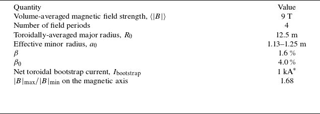
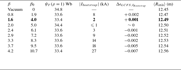
3. Operating design point
The Infinity Two FPP design is a quasi-isodynamic configuration with stellarator symmetry (Dewar & Hudson Reference Dewar and Hudson1998). The main characteristics of the target $800\ \textrm{MW}$
DT fusion power operating point are summarised in table 1, including the configuration’s volume-averaged magnetic field, toroidally averaged major radius, the effective minor radius, the volume average
$800\ \textrm{MW}$
DT fusion power operating point are summarised in table 1, including the configuration’s volume-averaged magnetic field, toroidally averaged major radius, the effective minor radius, the volume average $\beta$
, the on-axis
$\beta$
, the on-axis $\beta _0$
and the estimated net toroidal bootstrap current. External heating is envisage to be provided by electron cyclotron resonance heating at 8.42 T. Continuous pellet fuelling is also required (Guttenfelder et al. Reference Guttenfelder2025). The edge transform approaches
$\beta _0$
and the estimated net toroidal bootstrap current. External heating is envisage to be provided by electron cyclotron resonance heating at 8.42 T. Continuous pellet fuelling is also required (Guttenfelder et al. Reference Guttenfelder2025). The edge transform approaches ${\iota\kern-3.5pt\def\negativespace{}\mbox{-}\kern0.5pt}=4/5$
. By purposely avoiding
${\iota\kern-3.5pt\def\negativespace{}\mbox{-}\kern0.5pt}=4/5$
. By purposely avoiding ${\iota\kern-3.5pt\def\negativespace{}\mbox{-}\kern0.5pt}=1$
, the Infinity Two stellarator avoids the issues related to having multiple low-order resonances (1/1, 2/2, 3/3, etc.) that W7-X has had to deal with to ensure symmetric loading on the divertor plates (Andreeva et al. Reference Andreeva, Bräuer, Endler, Kisslinger and Igitkhanov2004; Kisslinger & Andreeva Reference Kisslinger and Andreeva2005; Jakubowski et al. Reference Jakubowski2021). The only source of current considered in this modelling is the bootstrap current, and it increases the edge transform by
${\iota\kern-3.5pt\def\negativespace{}\mbox{-}\kern0.5pt}=1$
, the Infinity Two stellarator avoids the issues related to having multiple low-order resonances (1/1, 2/2, 3/3, etc.) that W7-X has had to deal with to ensure symmetric loading on the divertor plates (Andreeva et al. Reference Andreeva, Bräuer, Endler, Kisslinger and Igitkhanov2004; Kisslinger & Andreeva Reference Kisslinger and Andreeva2005; Jakubowski et al. Reference Jakubowski2021). The only source of current considered in this modelling is the bootstrap current, and it increases the edge transform by $\Delta {\iota\kern-3.5pt\def\negativespace{}\mbox{-}\kern0.5pt}\approx +0.001$
compared with the same finite-
$\Delta {\iota\kern-3.5pt\def\negativespace{}\mbox{-}\kern0.5pt}\approx +0.001$
compared with the same finite- $\beta$
equilibrium with no net toroidal current.
$\beta$
equilibrium with no net toroidal current.
Table 1. Properties of the Infinity Two FPP stellarator configuration discussed in this article. ${}^{*}$
This bootstrap current calculation uses the multi-species SFINCS evaluations.
${}^{*}$
This bootstrap current calculation uses the multi-species SFINCS evaluations.
The profiles used in this modelling, shown in figure 1, were informed by the high-fidelity modelling detailed by Guttenfelder et al. (Reference Guttenfelder2025). The density profile is flat for $\rho \leqslant 0.5$
with an on-axis value of
$\rho \leqslant 0.5$
with an on-axis value of ${\sim} 2.46\times 10^{20}\ \textrm{m}^{-3}$
and an edge density of
${\sim} 2.46\times 10^{20}\ \textrm{m}^{-3}$
and an edge density of ${\sim} 6.15\times 10^{19}\ \textrm{m}^{-3}$
. The on-axis temperatures of the electrons is
${\sim} 6.15\times 10^{19}\ \textrm{m}^{-3}$
. The on-axis temperatures of the electrons is ${\sim} 17.26\ \textrm{keV}$
and the ions are at
${\sim} 17.26\ \textrm{keV}$
and the ions are at ${\sim} 13.81\ \textrm{keV}$
. The edge temperature for both ions and electrons is
${\sim} 13.81\ \textrm{keV}$
. The edge temperature for both ions and electrons is $100\ \textrm{eV}$
. The non-zero gradient of the ion-temperature profile is not present in the refined high-fidelity profiles (see e.g. figure 9 of Guttenfelder et al. (Reference Guttenfelder2025)), and its influence on the estimates of the bootstrap current density and MHD stability near the axis is negligible. The coil set for this configuration is described by Hegna et al. (Reference Hegna2025) and shown in figure 2. It reproduces the desired target magnetic field to a high degree of accuracy with 12 coils per field period (48 coils total), while simultaneously satisfying engineering constraints on minimum coil–coil and coil–plasma distances, maximum curvature of the coils, and sufficient space for other components around the plasma. A single-filament version of the coil set was used for the modelling in this work. The interpolated magnetic grid for free-boundary VMEC evaluations was defined to span from
$100\ \textrm{eV}$
. The non-zero gradient of the ion-temperature profile is not present in the refined high-fidelity profiles (see e.g. figure 9 of Guttenfelder et al. (Reference Guttenfelder2025)), and its influence on the estimates of the bootstrap current density and MHD stability near the axis is negligible. The coil set for this configuration is described by Hegna et al. (Reference Hegna2025) and shown in figure 2. It reproduces the desired target magnetic field to a high degree of accuracy with 12 coils per field period (48 coils total), while simultaneously satisfying engineering constraints on minimum coil–coil and coil–plasma distances, maximum curvature of the coils, and sufficient space for other components around the plasma. A single-filament version of the coil set was used for the modelling in this work. The interpolated magnetic grid for free-boundary VMEC evaluations was defined to span from $R\approx 8.44$
–
$R\approx 8.44$
– $16.59\ \textrm{m}$
,
$16.59\ \textrm{m}$
, $Z\approx -3.78$
–
$Z\approx -3.78$
– $ 3.78\ \textrm{m}$
, and with 180 grids in the toroidal direction over one field period. The magnetic grid for HINT evaluations used the same radial and vertical limits, but all three grids were defined to have 256 steps. Prior to using the profiles based on the high-fidelity modelling (Guttenfelder et al. Reference Guttenfelder2025), a pressure profile that was more peaked had been assumed for the fixed-boundary version of this configuration. The coilset had been designed for those peaked profiles (not shown). The mirror-like
$ 3.78\ \textrm{m}$
, and with 180 grids in the toroidal direction over one field period. The magnetic grid for HINT evaluations used the same radial and vertical limits, but all three grids were defined to have 256 steps. Prior to using the profiles based on the high-fidelity modelling (Guttenfelder et al. Reference Guttenfelder2025), a pressure profile that was more peaked had been assumed for the fixed-boundary version of this configuration. The coilset had been designed for those peaked profiles (not shown). The mirror-like $|B|$
on the last closed flux surface in Boozer coordinates is shown in figure 3. In the left column of figure 4, the spectrum of the field strength
$|B|$
on the last closed flux surface in Boozer coordinates is shown in figure 3. In the left column of figure 4, the spectrum of the field strength $|B|$
in straight field line (Boozer) coordinates for the original fixed-boundary target equilibrium (solid lines) is compared with the corresponding spectrum for the free-boundary VMEC solution (dashed lines). The boundary of the free-boundary solution was adjusted to account for the presence of the edge island structures, as described in Appendix C. The rank of the modes was determined by their individual maximum-absolute value across the entire radial profile. The x-axis for this figure is the effective minor radius,
$|B|$
in straight field line (Boozer) coordinates for the original fixed-boundary target equilibrium (solid lines) is compared with the corresponding spectrum for the free-boundary VMEC solution (dashed lines). The boundary of the free-boundary solution was adjusted to account for the presence of the edge island structures, as described in Appendix C. The rank of the modes was determined by their individual maximum-absolute value across the entire radial profile. The x-axis for this figure is the effective minor radius, $r_{\rm eff}=a_0 \sqrt {s}$
. The y-axis is a
$r_{\rm eff}=a_0 \sqrt {s}$
. The y-axis is a $\pm$
log scale with unequal upper and lower limits. The rank and general shape of each of the top 20 modes of the spectrum agree well between the fixed- and free- boundary solutions, in spite of the slight change in the placement of the boundary. Furthermore, the harmonics from coil ripple (
$\pm$
log scale with unequal upper and lower limits. The rank and general shape of each of the top 20 modes of the spectrum agree well between the fixed- and free- boundary solutions, in spite of the slight change in the placement of the boundary. Furthermore, the harmonics from coil ripple ( $n = 12$
) are not evident. The
$n = 12$
) are not evident. The $(m,n) = (0,12)$
component is smaller than
$(m,n) = (0,12)$
component is smaller than $10^{-3}$
at the magnetic axis of the VMEC solution. The right column of figure 4 is similar to the left, except that the Boozer spectrum has been replaced by that of the MHD solution with pressure profiles based on figure 1. The top 20 modes are the same as those in the left column, although the rank has changed among the last four. In spite of the different pressure profiles, the spectrum is remarkably similar, suggesting that the modifications to the spectrum due to finite-
$10^{-3}$
at the magnetic axis of the VMEC solution. The right column of figure 4 is similar to the left, except that the Boozer spectrum has been replaced by that of the MHD solution with pressure profiles based on figure 1. The top 20 modes are the same as those in the left column, although the rank has changed among the last four. In spite of the different pressure profiles, the spectrum is remarkably similar, suggesting that the modifications to the spectrum due to finite- $\beta$
effects may be small.
$\beta$
effects may be small.
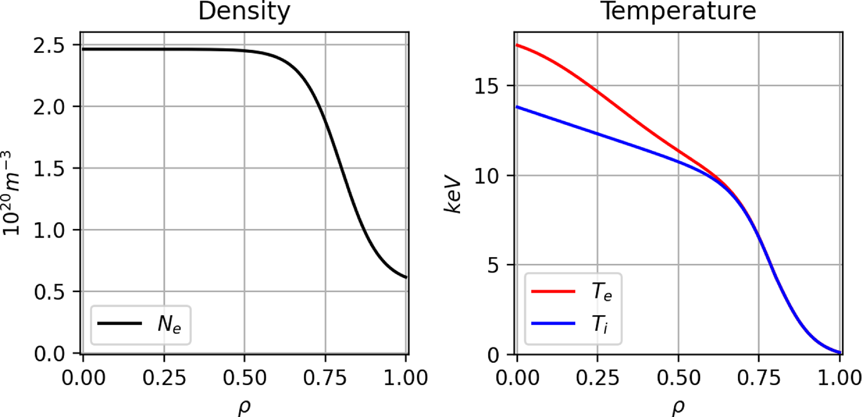
Figure 1. Plasma profiles informed by high-fidelity transport modelling (Guttenfelder et al. Reference Guttenfelder2025).
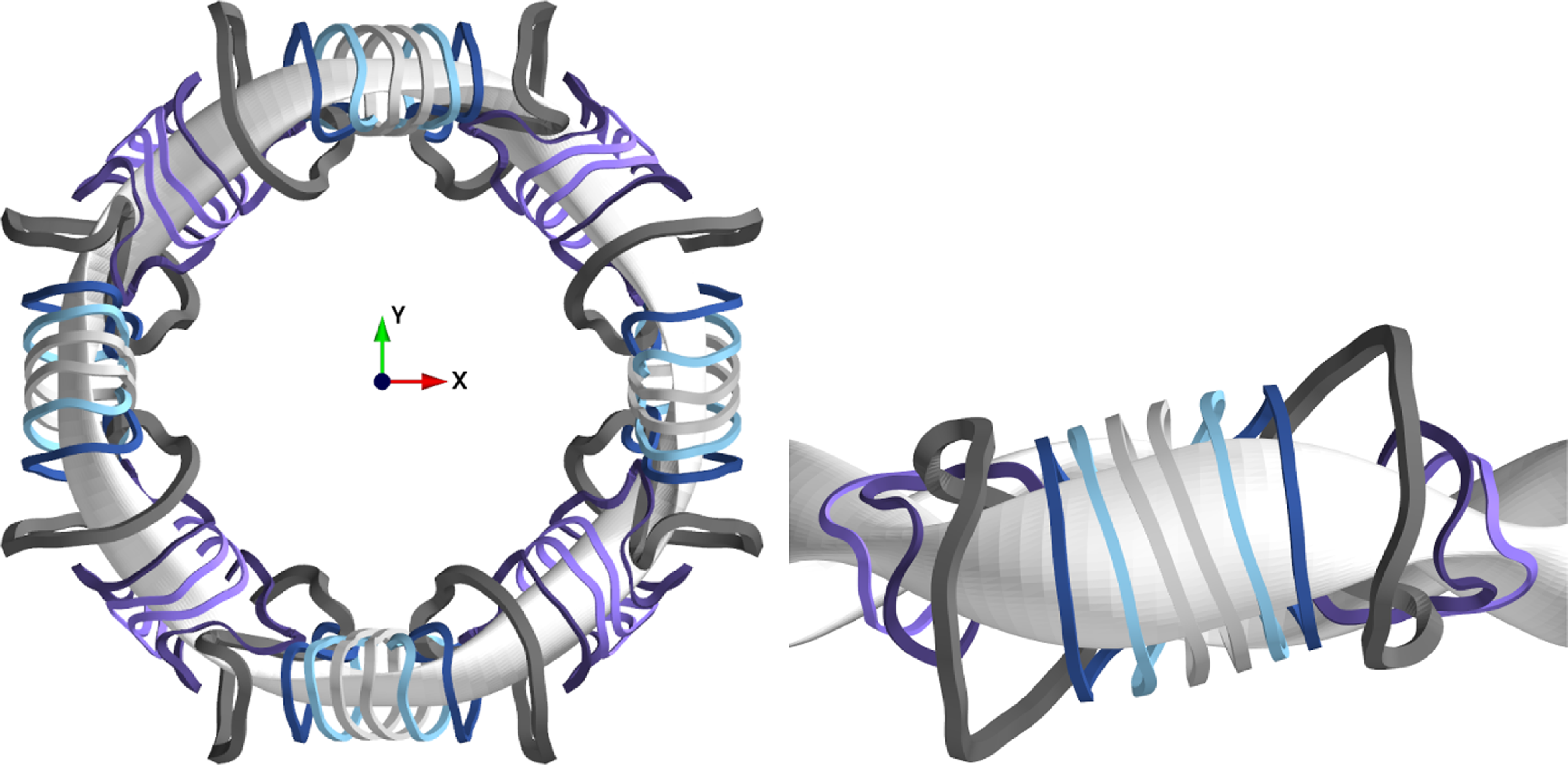
Figure 2. Left, top down view of a coil set with finite build for Infinity Two. There are twelve coils per field period. Right, side view of Infinity Two’s coil set.
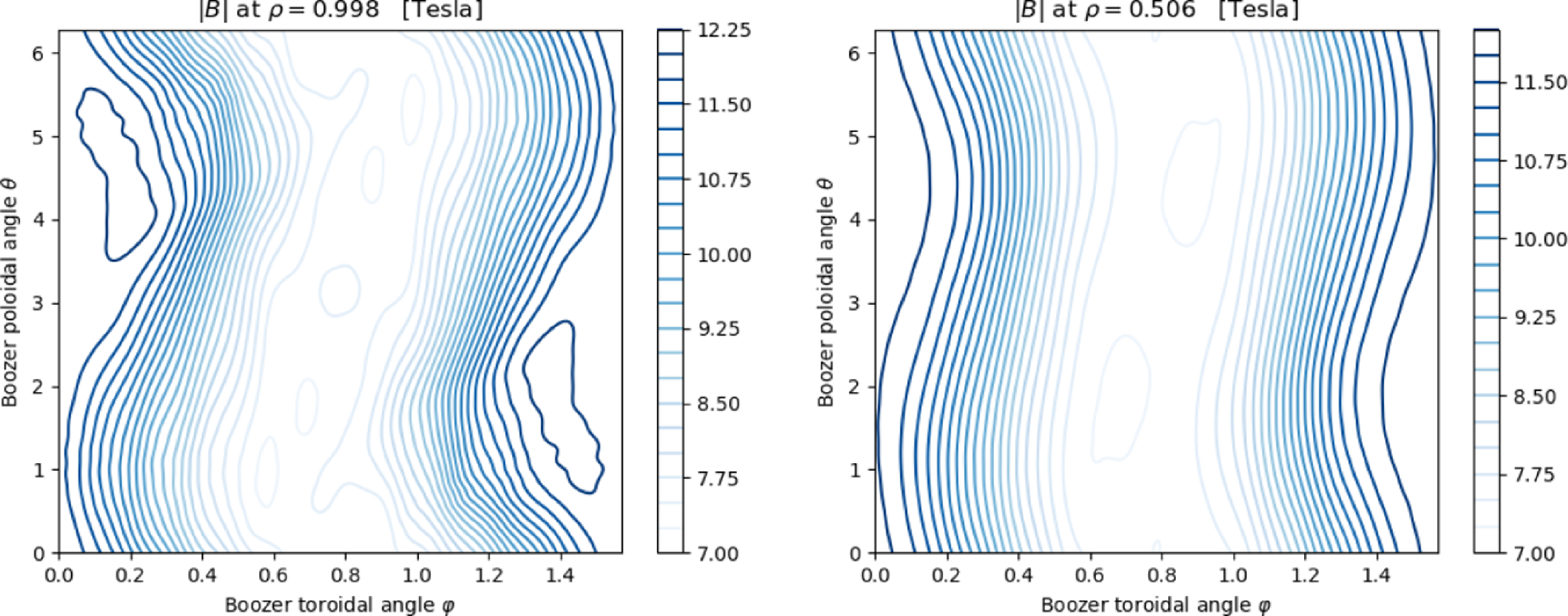
Figure 3. Contour plot of $|B|$
close to the last closed flux surface (left) and the mid-radius (right) of the
$|B|$
close to the last closed flux surface (left) and the mid-radius (right) of the $\beta =1.6\ \%$
free-boundary VMEC MHD solution. The x- and y-axes correspond to the toroidal and poloidal angles, respectively, and span a single field period.
$\beta =1.6\ \%$
free-boundary VMEC MHD solution. The x- and y-axes correspond to the toroidal and poloidal angles, respectively, and span a single field period.
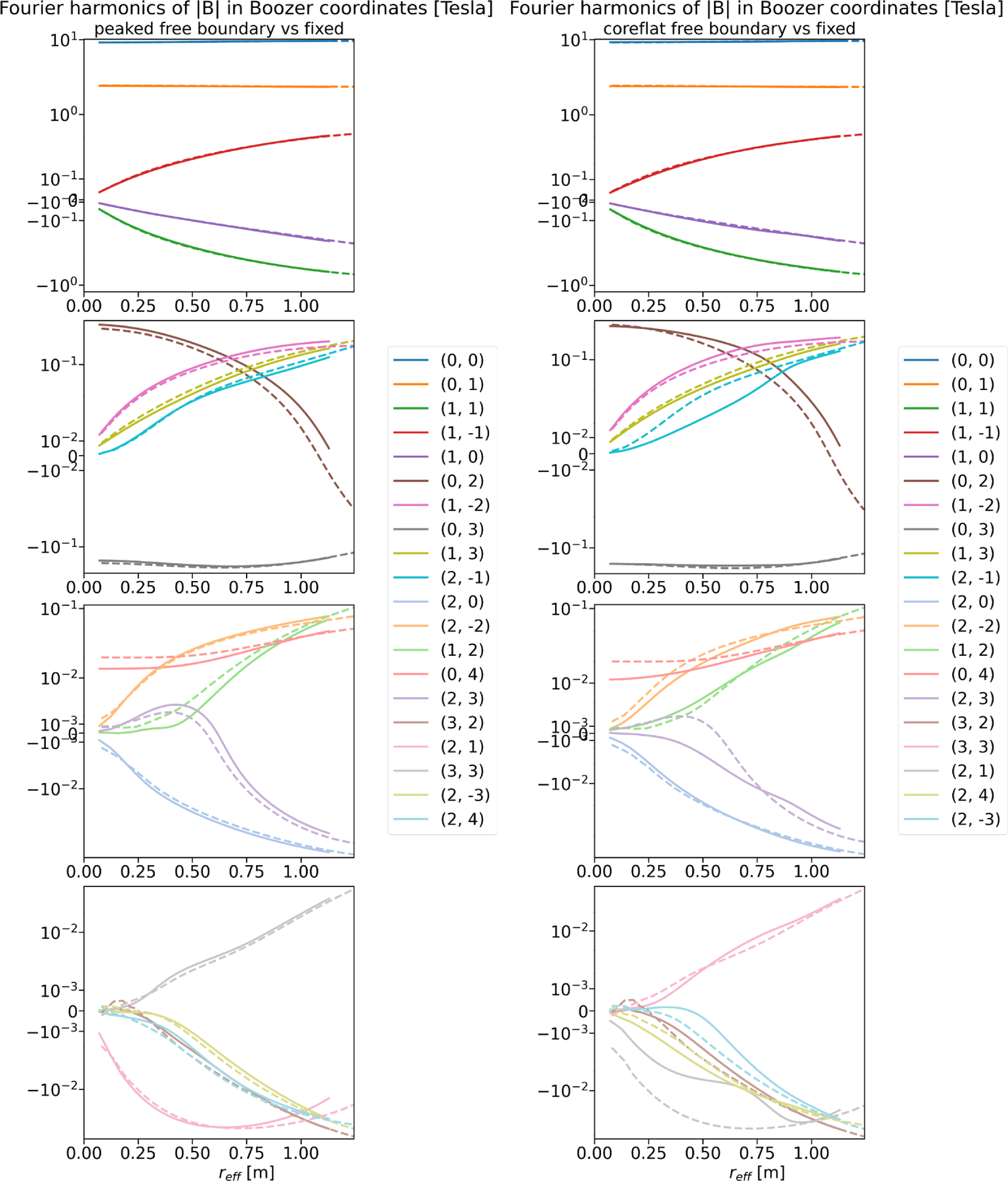
Figure 4. Radial profiles of the largest 20 spectral components of $B$
in Boozer coordinates. Left column, the spectrum of the target configuration from the fixed-boundary optimisation procedure is shown as solid lines. The spectrum for the free boundary configuration is shown as dashed lines with the same colour scheme as the fixed boundary spectrum. The y-axis is a logarithmic scale (sign-preserving) and the x-axis is
$B$
in Boozer coordinates. Left column, the spectrum of the target configuration from the fixed-boundary optimisation procedure is shown as solid lines. The spectrum for the free boundary configuration is shown as dashed lines with the same colour scheme as the fixed boundary spectrum. The y-axis is a logarithmic scale (sign-preserving) and the x-axis is $\rho =\sqrt {\psi _t/\psi _{t,\textrm{LCFS}}}$
. Numbers in the legend indicate the poloidal and toroidal mode numbers (
$\rho =\sqrt {\psi _t/\psi _{t,\textrm{LCFS}}}$
. Numbers in the legend indicate the poloidal and toroidal mode numbers ( $m, n$
). Right column, the spectrum of the target configuration as solid lines compared with the spectrum of the free boundary solution with the profiles from figure 1. The same 20 modes populate the top ranks, but the order of the last four is different.
$m, n$
). Right column, the spectrum of the target configuration as solid lines compared with the spectrum of the free boundary solution with the profiles from figure 1. The same 20 modes populate the top ranks, but the order of the last four is different.
A Poincaré map at the $1/2$
-field period location was generated with line-following based on the vacuum fields generated by the coil set using the Julia-based MagneticFieldToolkit (Faber & Bader Reference Faber and Bader2024a). The result in figure 5 demonstrates that good flux surfaces exist in this configuration even without plasma, an essential fact required for a stellarator.
$1/2$
-field period location was generated with line-following based on the vacuum fields generated by the coil set using the Julia-based MagneticFieldToolkit (Faber & Bader Reference Faber and Bader2024a). The result in figure 5 demonstrates that good flux surfaces exist in this configuration even without plasma, an essential fact required for a stellarator.
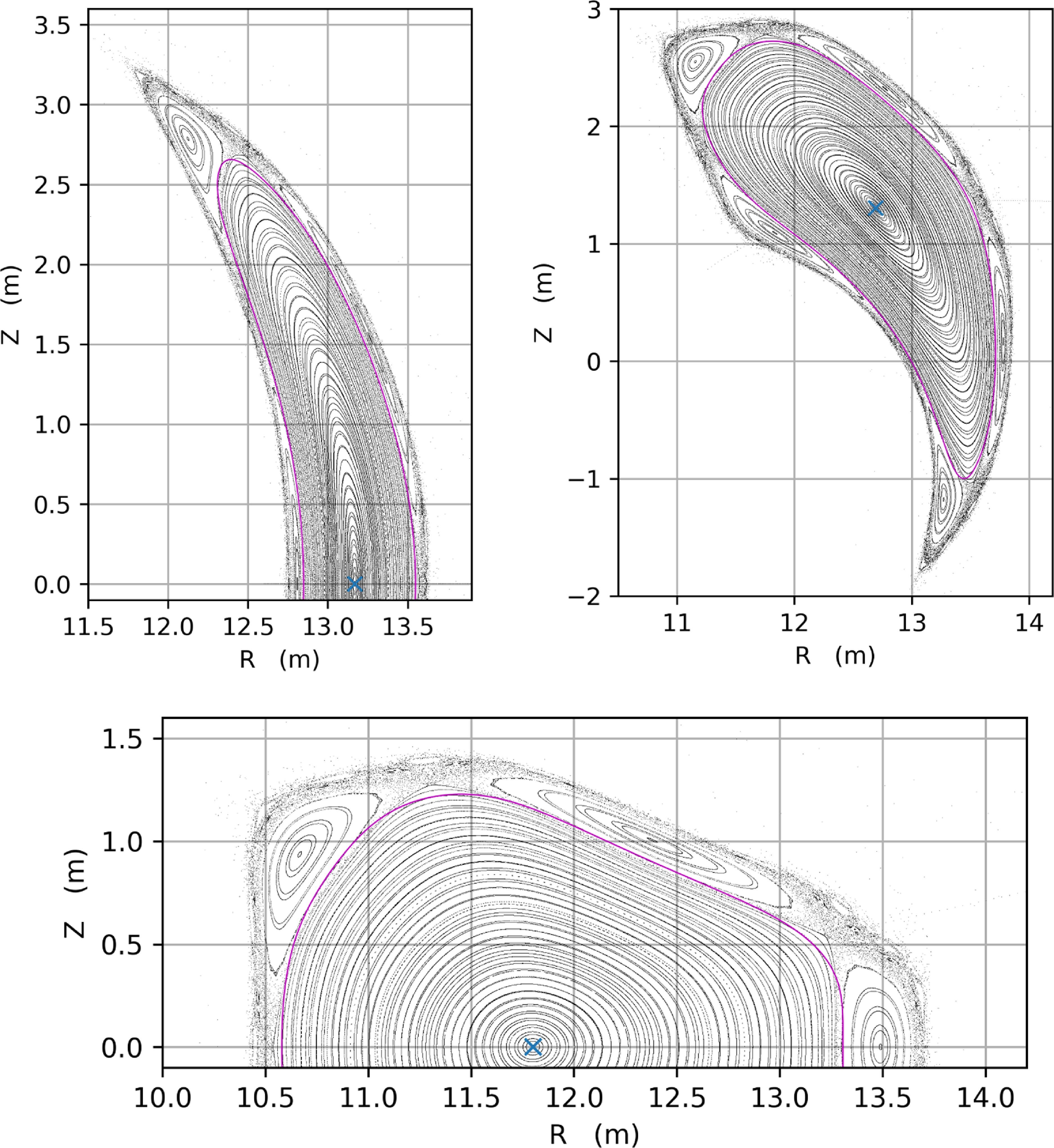
Figure 5. Black points, Poincaré map at $\phi =0$
,
$\phi =0$
, $\pi /8$
and
$\pi /8$
and $\pi /4$
for the magnetic field generated only by coils. Well-formed closed flux surfaces form the core of the confinement region and an
$\pi /4$
for the magnetic field generated only by coils. Well-formed closed flux surfaces form the core of the confinement region and an ${\iota\kern-3.5pt\def\negativespace{}\mbox{-}\kern0.5pt}=4/5$
island is in the edge. Magenta line and blue ×, the LCFS and magnetic axis of the free boundary vacuum VMEC solution, respectively.
${\iota\kern-3.5pt\def\negativespace{}\mbox{-}\kern0.5pt}=4/5$
island is in the edge. Magenta line and blue ×, the LCFS and magnetic axis of the free boundary vacuum VMEC solution, respectively.
Two methods were used to evaluate the vacuum rotational transform profile ${\iota\kern-3.5pt\def\negativespace{}\mbox{-}\kern0.5pt}_{\textrm{vac}}$
generated solely by energising the coilset. The first is via line-following, where
${\iota\kern-3.5pt\def\negativespace{}\mbox{-}\kern0.5pt}_{\textrm{vac}}$
generated solely by energising the coilset. The first is via line-following, where ${\iota\kern-3.5pt\def\negativespace{}\mbox{-}\kern0.5pt}_{\textrm{vac}}$
is estimated by (1.2) for several field lines launched at the
${\iota\kern-3.5pt\def\negativespace{}\mbox{-}\kern0.5pt}_{\textrm{vac}}$
is estimated by (1.2) for several field lines launched at the $Z=0$
,
$Z=0$
, $\phi =0$
plane with the value of
$\phi =0$
plane with the value of $R$
varied to scan across the minor radius. The second evaluation of
$R$
varied to scan across the minor radius. The second evaluation of ${\iota\kern-3.5pt\def\negativespace{}\mbox{-}\kern0.5pt}_{\textrm{vac}}$
is from the free-boundary VMEC solution which calculates the transform as
${\iota\kern-3.5pt\def\negativespace{}\mbox{-}\kern0.5pt}_{\textrm{vac}}$
is from the free-boundary VMEC solution which calculates the transform as ${\iota\kern-3.5pt\def\negativespace{}\mbox{-}\kern0.5pt} \equiv\textrm{d}\psi _p/\textrm{d}\psi _t$
, the ratio of the differential change in poloidal (
${\iota\kern-3.5pt\def\negativespace{}\mbox{-}\kern0.5pt} \equiv\textrm{d}\psi _p/\textrm{d}\psi _t$
, the ratio of the differential change in poloidal ( $\psi _p$
) and toroidal (
$\psi _p$
) and toroidal ( $\psi _t$
) magnetic fluxes enclosed within a surface. The two methods are compared in figure 6 and agree well, with differences noted near the magnetic axis, where VMEC results converge slowly with the number of surfaces in the radial grid NS. As described in Appendix B, this vacuum solution was converged with NS = 165, MPOL=NTOR = 14 and FTOL=1.5e-11. To achieve better on-axis convergence for the vacuum case, NS = 300 or higher may be required.
$\psi _t$
) magnetic fluxes enclosed within a surface. The two methods are compared in figure 6 and agree well, with differences noted near the magnetic axis, where VMEC results converge slowly with the number of surfaces in the radial grid NS. As described in Appendix B, this vacuum solution was converged with NS = 165, MPOL=NTOR = 14 and FTOL=1.5e-11. To achieve better on-axis convergence for the vacuum case, NS = 300 or higher may be required.
Table 2. Relative concentrations of deuterium, tritium, helium, tungsten and neon for multi-species self-consistent bootstrap current evaluations.
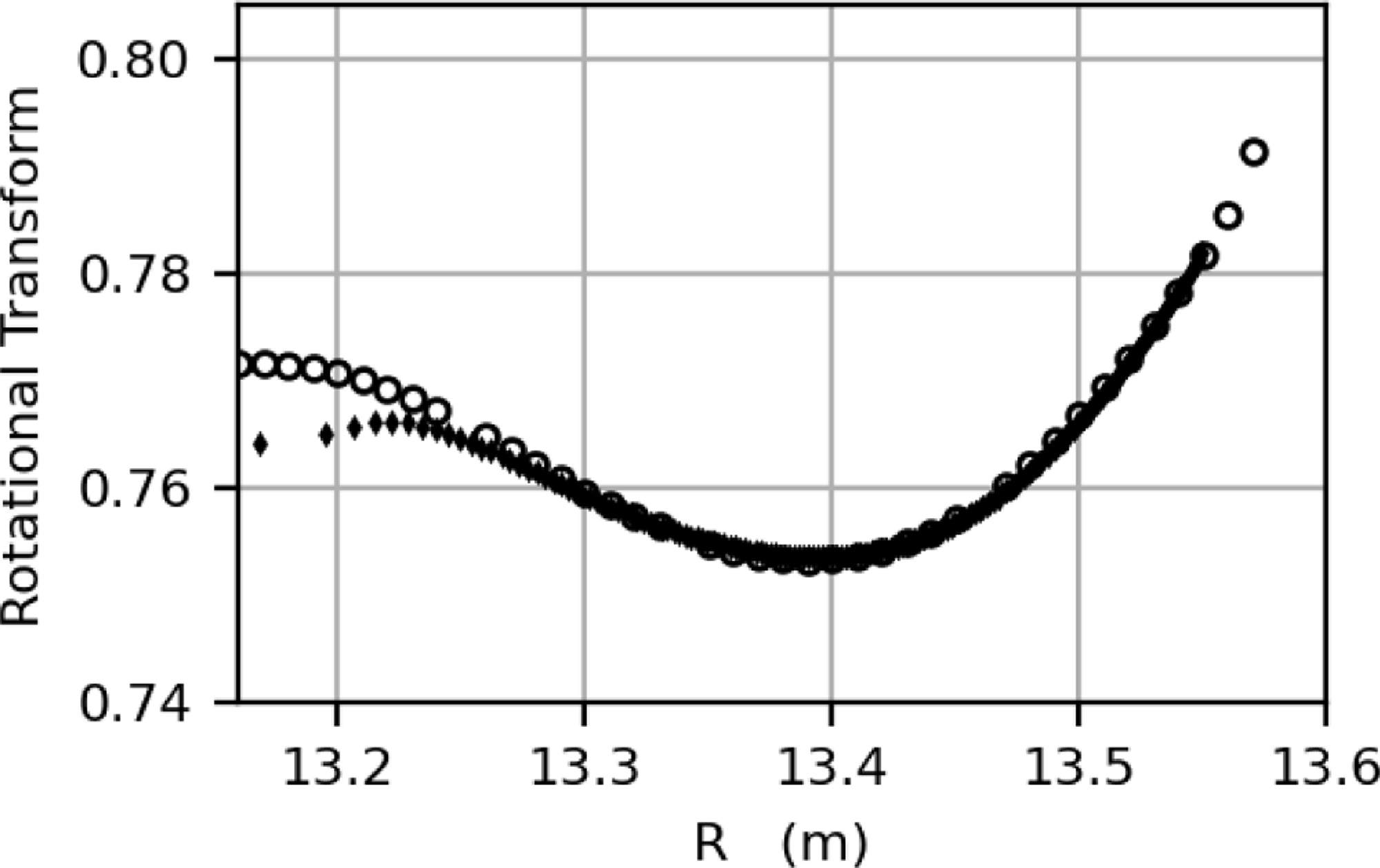
Figure 6. Comparison of rotational transform profiles for the vacuum configuration. The circles correspond to ${\iota\kern-3.5pt\def\negativespace{}\mbox{-}\kern0.5pt}_{\textrm{vac}}$
computed via field line tracing and the diamonds correspond to
${\iota\kern-3.5pt\def\negativespace{}\mbox{-}\kern0.5pt}_{\textrm{vac}}$
computed via field line tracing and the diamonds correspond to ${\iota\kern-3.5pt\def\negativespace{}\mbox{-}\kern0.5pt}_{\textrm{vac}}$
computed from the VMEC free-boundary equilibrium.
${\iota\kern-3.5pt\def\negativespace{}\mbox{-}\kern0.5pt}_{\textrm{vac}}$
computed from the VMEC free-boundary equilibrium.
Self-consistent estimates of the bootstrap current for the profiles shown in figure 1 were established for the free-boundary configuration. The left panel of figure 7 shows the profiles of the neoclassical bootstrap current for a two-species electron–hydrogen plasma with $T_H = T_i$
,
$T_H = T_i$
, $N_H = N_e$
from figure 1. A multi-species scenario which more closely models that of a burning fusion reactor is also considered. The relative ratios of the plasma species are listed in table 2, and all ion species are assumed to be in thermal equilibrium (for all ions ‘X’,
$N_H = N_e$
from figure 1. A multi-species scenario which more closely models that of a burning fusion reactor is also considered. The relative ratios of the plasma species are listed in table 2, and all ion species are assumed to be in thermal equilibrium (for all ions ‘X’, $T_X = T_i$
from figure 1). The ambipolar radial electric field solution for both of these scenarios is shown in the right panel of figure 7. In the two-species case, the ion-root is the only stable solution found at all radii, except for the points nearest the magnetic axis (
$T_X = T_i$
from figure 1). The ambipolar radial electric field solution for both of these scenarios is shown in the right panel of figure 7. In the two-species case, the ion-root is the only stable solution found at all radii, except for the points nearest the magnetic axis ( $\rho \leqslant 0.10$
) where the electron-root was found to also be stable. In this specific case, the evaluation of (D.2) predicts that the ion-root is the most likely solution. Even so, the effect on the bootstrap current would likely be minimal as the differences in parallel current are small at
$\rho \leqslant 0.10$
) where the electron-root was found to also be stable. In this specific case, the evaluation of (D.2) predicts that the ion-root is the most likely solution. Even so, the effect on the bootstrap current would likely be minimal as the differences in parallel current are small at $\rho =0.05$
and negligible at
$\rho =0.05$
and negligible at $\rho =0.10$
(figure 7, left). In the multi-species case, only one root is stable at all radii and the solution near the core is positive for
$\rho =0.10$
(figure 7, left). In the multi-species case, only one root is stable at all radii and the solution near the core is positive for $\rho \leqslant 0.1$
, which may help expel high-Z impurities near the axis. The total bootstrap current at the target operating point is estimated to be small. In the two-species case,
$\rho \leqslant 0.1$
, which may help expel high-Z impurities near the axis. The total bootstrap current at the target operating point is estimated to be small. In the two-species case, $I_\textrm{bootstrap} \approx 2\ \textrm{kA}$
and in the multi-species case,
$I_\textrm{bootstrap} \approx 2\ \textrm{kA}$
and in the multi-species case, $I_\textrm{bootstrap} \approx 1\ \textrm{kA}$
. The effect of the total bootstrap current at
$I_\textrm{bootstrap} \approx 1\ \textrm{kA}$
. The effect of the total bootstrap current at $\beta =1.6\,\%$
is to add to the rotational transform.
$\beta =1.6\,\%$
is to add to the rotational transform.
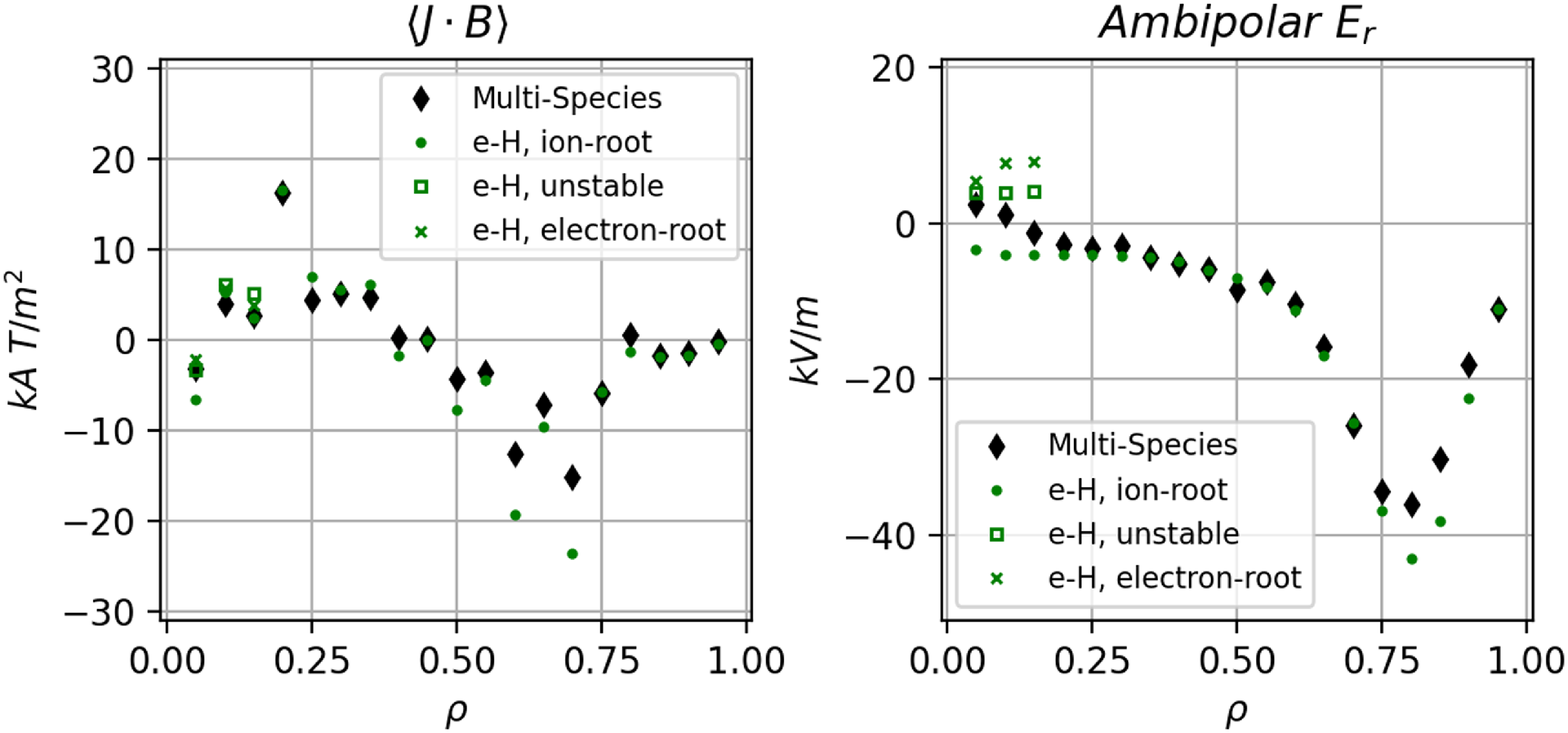
Figure 7. Left panel, the neoclassical bootstrap current $\langle J \cdot B\rangle$
for two-species electron-hydrogen plasmas (green markers) and multi-species plasmas (black diamonds) with profiles of figure 1 and relative ratios listed in table 2 for the multi-species case. Right panel, ambipolar radial electric field solution for cases shown in the left panel. The stable solution is the ion-root for the two species (e–H) case.
$\langle J \cdot B\rangle$
for two-species electron-hydrogen plasmas (green markers) and multi-species plasmas (black diamonds) with profiles of figure 1 and relative ratios listed in table 2 for the multi-species case. Right panel, ambipolar radial electric field solution for cases shown in the left panel. The stable solution is the ion-root for the two species (e–H) case.
The adiabatic invariant is a measure of the qausi-isodynamic quality of the configuration, defined by
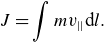 \begin{equation} J = \int m v_{||} \textrm{d}l . \end{equation}
In the ideal limit, $J = J(\psi )$
, the
$J = J(\psi )$
, the $J$
contours correspond to surfaces of constant radius. In figure 8, the contours of adiabatic invariant, (3.1), are shown for different choices of the pitch angle variable
$J$
contours correspond to surfaces of constant radius. In figure 8, the contours of adiabatic invariant, (3.1), are shown for different choices of the pitch angle variable $\lambda _n$
for the fixed-boundary
$\lambda _n$
for the fixed-boundary $\beta =1.6\,\%$
equilibrium (top row), the free-boundary
$\beta =1.6\,\%$
equilibrium (top row), the free-boundary $\beta =1.6\,\%$
equilibrium (middle row) and the free-boundary vacuum solution (bottom row). Here,
$\beta =1.6\,\%$
equilibrium (middle row) and the free-boundary vacuum solution (bottom row). Here, $\lambda _n^2 = B_\textrm{max}(1 - \mu B_\textrm{min}/\mathcal {E})/(B_\textrm{max} - B_\textrm{min})$
denotes a particle with energy
$\lambda _n^2 = B_\textrm{max}(1 - \mu B_\textrm{min}/\mathcal {E})/(B_\textrm{max} - B_\textrm{min})$
denotes a particle with energy $\mathcal {E}$
and magnetic moment
$\mathcal {E}$
and magnetic moment $\mu$
moving along a field line with minimum (maximum) value of magnetic field strength given by
$\mu$
moving along a field line with minimum (maximum) value of magnetic field strength given by $B_\textrm{min}$
(
$B_\textrm{min}$
( $B_\textrm{max}$
). Here,
$B_\textrm{max}$
). Here, $\lambda _n \rightarrow 0$
denotes deeply trapped particles and
$\lambda _n \rightarrow 0$
denotes deeply trapped particles and $\lambda _n \rightarrow 1$
denotes barely trapped particles. In these plots in polar coordinates, the flux surface label
$\lambda _n \rightarrow 1$
denotes barely trapped particles. In these plots in polar coordinates, the flux surface label $\rho$
and the field line angle label
$\rho$
and the field line angle label $\alpha$
are mapped to the radial and angle coordinates, respectively.
$\alpha$
are mapped to the radial and angle coordinates, respectively.
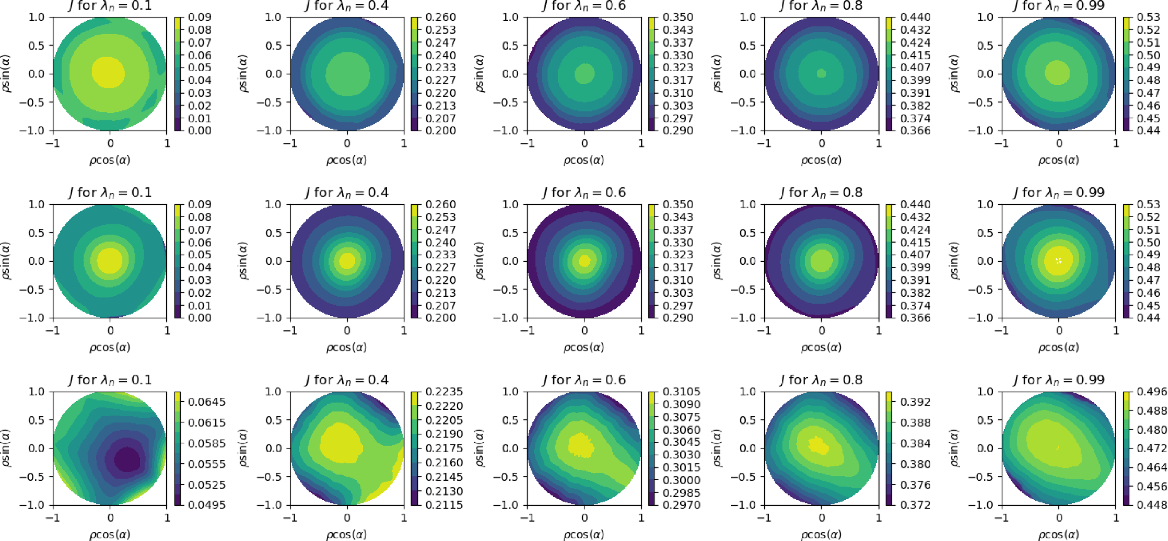
Figure 8. Polar plots ( $\rho \ \text{versus}\ \theta$
) of the second adiabatic invariant,
$\rho \ \text{versus}\ \theta$
) of the second adiabatic invariant, $J_\textrm{inv}$
for a range of bounce parameter,
$J_\textrm{inv}$
for a range of bounce parameter, $\lambda$
. Top row, fixed-boundary
$\lambda$
. Top row, fixed-boundary $\beta =1.6\,\%$
configuration; middle row, free-boundary solution at
$\beta =1.6\,\%$
configuration; middle row, free-boundary solution at $\beta =1.6\,\%$
; bottom row, free-boundary vacuum solution. Good poloidal closure of the
$\beta =1.6\,\%$
; bottom row, free-boundary vacuum solution. Good poloidal closure of the $J_{inv}$
contours is seen in both the fixed- and free- boundary finite beta solutions. Minor differences can be seen between the two finite beta solutions. The quality of the poloidal closure is degraded somewhat in the vacuum solution.
$J_{inv}$
contours is seen in both the fixed- and free- boundary finite beta solutions. Minor differences can be seen between the two finite beta solutions. The quality of the poloidal closure is degraded somewhat in the vacuum solution.
Evaluations with HINT at the $\beta = 1.6\,\%$
operating point were performed. The pressure profiles in the HINT simulation were parabolic in
$\beta = 1.6\,\%$
operating point were performed. The pressure profiles in the HINT simulation were parabolic in $\rho$
, and the peak value was adjusted to match
$\rho$
, and the peak value was adjusted to match $\beta =1.6\,\%$
of the operating point. Poincaré maps generated with the HINT solution are shown in figure 9 as black dots. The enclosed toroidal flux of the VMEC solution was adjusted so that the LCFS of each simulation matched to within approximately 0.4 Wb. The LCFS of the free-boundary VMEC solution is shown in magenta, which lies close to the LCFS of the HINT solution just inside the O-points of the resonant
$\beta =1.6\,\%$
of the operating point. Poincaré maps generated with the HINT solution are shown in figure 9 as black dots. The enclosed toroidal flux of the VMEC solution was adjusted so that the LCFS of each simulation matched to within approximately 0.4 Wb. The LCFS of the free-boundary VMEC solution is shown in magenta, which lies close to the LCFS of the HINT solution just inside the O-points of the resonant $(m,n)=(5,4)$
island that defines the boundary of this configuration. The magnetic axis of the VMEC solution, shown as a blue ‘X’ is well aligned with the axis of the HINT solution. In the same figure, the blue circles represent selected surfaces of the vacuum solution (magnetic axis, O-points of the island and two surfaces close to the plasma/island interface).
$(m,n)=(5,4)$
island that defines the boundary of this configuration. The magnetic axis of the VMEC solution, shown as a blue ‘X’ is well aligned with the axis of the HINT solution. In the same figure, the blue circles represent selected surfaces of the vacuum solution (magnetic axis, O-points of the island and two surfaces close to the plasma/island interface).
The edge ${\iota\kern-3.5pt\def\negativespace{}\mbox{-}\kern0.5pt}= 4/5$
island is robustly present, and has moved only slightly from its vacuum position, a combination of both a small-yet-finite pressure-driven Shafranov shift (which can also be seen as a shift in the magnetic axis from its vacuum location) and a very small change in the rotational transform, which modifies the location of the
${\iota\kern-3.5pt\def\negativespace{}\mbox{-}\kern0.5pt}= 4/5$
island is robustly present, and has moved only slightly from its vacuum position, a combination of both a small-yet-finite pressure-driven Shafranov shift (which can also be seen as a shift in the magnetic axis from its vacuum location) and a very small change in the rotational transform, which modifies the location of the ${\iota\kern-3.5pt\def\negativespace{}\mbox{-}\kern0.5pt}$
-resonance location in the radial direction. The connection length of the field lines, the rotational transform and fractal dimension were monitored for indications of the formation of islands and stochastic regions. In the core portion of the plasma column, no regions of chaos or internal islands larger than 0.5 cm have formed and pressure contours overlap with the Poincaré maps (not shown).
${\iota\kern-3.5pt\def\negativespace{}\mbox{-}\kern0.5pt}$
-resonance location in the radial direction. The connection length of the field lines, the rotational transform and fractal dimension were monitored for indications of the formation of islands and stochastic regions. In the core portion of the plasma column, no regions of chaos or internal islands larger than 0.5 cm have formed and pressure contours overlap with the Poincaré maps (not shown).
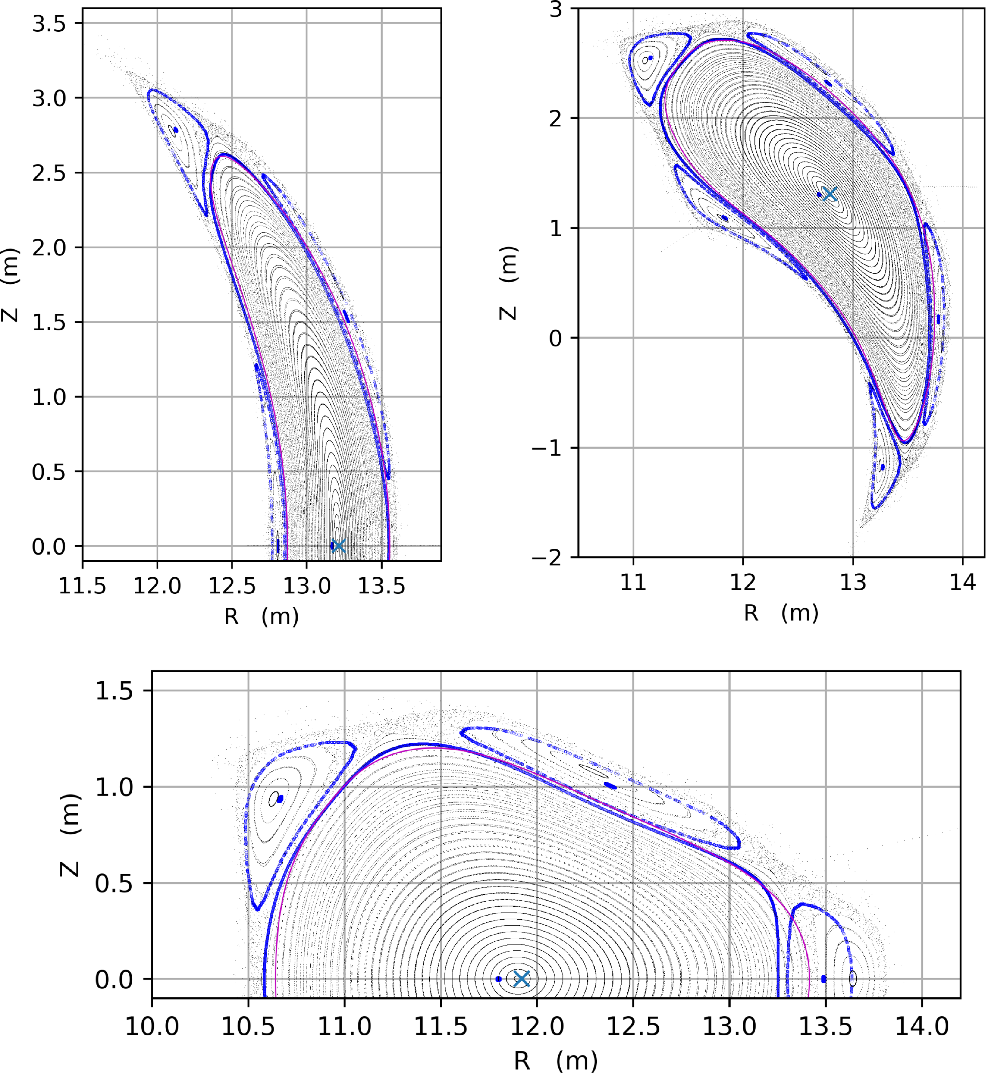
Figure 9. Poincaré maps from HINT simulation for $\phi =0$
,
$\phi =0$
, $\pi /8$
and
$\pi /8$
and $\pi /4$
at the
$\pi /4$
at the $\beta =1.6\,\%$
operating point shown as black points. The axis of the plasma column and island at vacuum and two surfaces close to the plasma/island interface in vacuum are shown in blue. The blue ‘X’ is the magnetic axis of the finite
$\beta =1.6\,\%$
operating point shown as black points. The axis of the plasma column and island at vacuum and two surfaces close to the plasma/island interface in vacuum are shown in blue. The blue ‘X’ is the magnetic axis of the finite $\beta =1.6\,\%$
VMEC evaluation. The last closed flux surface of the VMEC solution at the target operating point is shown as a magenta line.
$\beta =1.6\,\%$
VMEC evaluation. The last closed flux surface of the VMEC solution at the target operating point is shown as a magenta line.
4. Feasibility of the operating point
To assess the feasibility of reaching the $\beta = 1.6 \,\%$
operating point, along with the equilibrium and stability properties around the design point, a series of test scenarios were developed as a proxy for low- to high-
$\beta = 1.6 \,\%$
operating point, along with the equilibrium and stability properties around the design point, a series of test scenarios were developed as a proxy for low- to high- $\beta$
operation. While not a true pilot-plant scenario development exercise, it provides insight into the robustness, stability and feasibility expected of the operating design point. The test scenarios assume the same temperature profiles as the target operating point. The shapes of the density profiles are retained, but the magnitude of the density profiles was scaled down/up. This effectively scales the operating plasma pressure,
$\beta$
operation. While not a true pilot-plant scenario development exercise, it provides insight into the robustness, stability and feasibility expected of the operating design point. The test scenarios assume the same temperature profiles as the target operating point. The shapes of the density profiles are retained, but the magnitude of the density profiles was scaled down/up. This effectively scales the operating plasma pressure, $\beta$
and
$\beta$
and $\beta _0$
by the same factor. For each scenario, the enclosed toroidal flux was adjusted to match the boundary of a corresponding HINT simulation with the same effective
$\beta _0$
by the same factor. For each scenario, the enclosed toroidal flux was adjusted to match the boundary of a corresponding HINT simulation with the same effective $\beta$
, as discussed in Appendix C. Next, the self-consistent bootstrap current profile was calculated with free-boundary VMEC solutions while the net toroidal flux was held constant. For simplicity, a two-species electron–hydrogen plasma was assumed in this scan. The radial profiles of the plasma pressure, bootstrap current density and rotational transform are shown in figure 10. Table 3 shows the variation of the net current, the change in
$\beta$
, as discussed in Appendix C. Next, the self-consistent bootstrap current profile was calculated with free-boundary VMEC solutions while the net toroidal flux was held constant. For simplicity, a two-species electron–hydrogen plasma was assumed in this scan. The radial profiles of the plasma pressure, bootstrap current density and rotational transform are shown in figure 10. Table 3 shows the variation of the net current, the change in ${\iota\kern-3.5pt\def\negativespace{}\mbox{-}\kern0.5pt}(s=1)$
due to the bootstrap current,
${\iota\kern-3.5pt\def\negativespace{}\mbox{-}\kern0.5pt}(s=1)$
due to the bootstrap current, $\Delta {\iota\kern-3.5pt\def\negativespace{}\mbox{-}\kern0.5pt}_\textrm{LCFS}$
, and the average radial location of the magnetic axis.
$\Delta {\iota\kern-3.5pt\def\negativespace{}\mbox{-}\kern0.5pt}_\textrm{LCFS}$
, and the average radial location of the magnetic axis.
Table 3. Global equilibrium properties as a function of increasing plasma density for an electron–hydrogen plasma. $\beta$
,
$\beta$
, $\beta _0$
, total bootstrap current, its effect on the edge transform and the toroidally averaged radius of the magnetic axis.
$\beta _0$
, total bootstrap current, its effect on the edge transform and the toroidally averaged radius of the magnetic axis.
The Shafranov shift is linear with $\beta$
, as expected, and the value of
$\beta$
, as expected, and the value of ${\iota\kern-3.5pt\def\negativespace{}\mbox{-}\kern0.5pt}\left (s=1\right )$
of the MHD solution is only slightly influenced by the net bootstrap current. It may be necessary to demonstrate control of the island O-point location and size, either through re-optimisation of the configuration, compensation with the actuation of a set of external control coils or combination of the two. The classical divertor design proposed by Bader et al. (Reference Bader2025) is anticipated to function with no need of extra control, but the local island backside divertor would likely require fine control to operate as intended. It is anticipated that it will be sufficient to control the island position and shape with actively controlled external island-control coils similar to the control and/or planar coils of W7-X (Risse et al. Reference Risse, Rummel, Bosch, Bykov, Carls, Füllenbach, Mönnich, Nagel and Schneider2018). The net current peaks when the density is scaled to aproximately half its nominal value. From this peak, it reduces until it is nearly completely eliminated at a test scenario with the density scaled by 125 %. At higher values of
${\iota\kern-3.5pt\def\negativespace{}\mbox{-}\kern0.5pt}\left (s=1\right )$
of the MHD solution is only slightly influenced by the net bootstrap current. It may be necessary to demonstrate control of the island O-point location and size, either through re-optimisation of the configuration, compensation with the actuation of a set of external control coils or combination of the two. The classical divertor design proposed by Bader et al. (Reference Bader2025) is anticipated to function with no need of extra control, but the local island backside divertor would likely require fine control to operate as intended. It is anticipated that it will be sufficient to control the island position and shape with actively controlled external island-control coils similar to the control and/or planar coils of W7-X (Risse et al. Reference Risse, Rummel, Bosch, Bykov, Carls, Füllenbach, Mönnich, Nagel and Schneider2018). The net current peaks when the density is scaled to aproximately half its nominal value. From this peak, it reduces until it is nearly completely eliminated at a test scenario with the density scaled by 125 %. At higher values of $\beta$
, the bootstrap current reverses direction and increases in magnitude.
$\beta$
, the bootstrap current reverses direction and increases in magnitude.
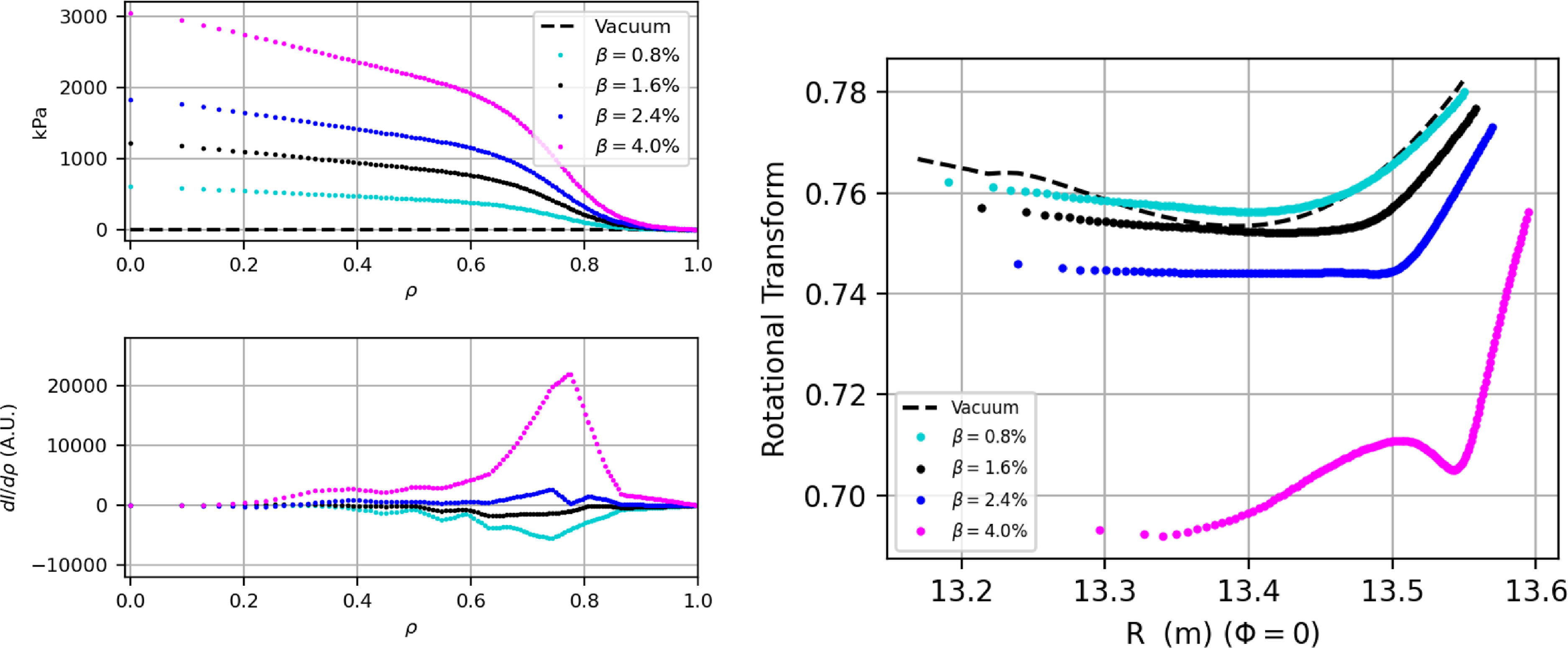
Figure 10. Left (top), plasma pressure profile for several test cases examined here. Left (bottom), toroidal current density profile for the same cases. Here, an electron–hydrogen plasma was assumed. Right, rotational transform profiles for the density scan.
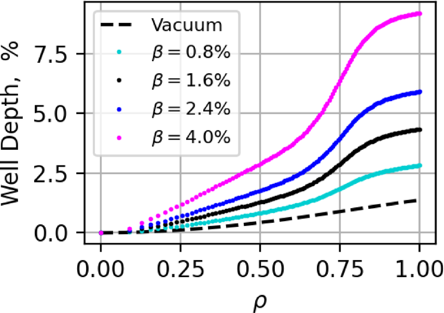
Figure 11. Magnetic well depth for test cases shown in figure 10. The magnetic well increases from ${\sim} 1.5\,\%$
in vacuum to above
${\sim} 1.5\,\%$
in vacuum to above $8\,\%$
at
$8\,\%$
at $\beta =4.0\,\%$
.
$\beta =4.0\,\%$
.
4.1. Low-density test scenarios, bootstrap current and ambipolar radial electric field
The ambipolar $E_r$
-solution is predicted to be entirely in the ion-root at the target operating point. In the test scenarios with an operating density below the target operating point, the ambipolar
$E_r$
-solution is predicted to be entirely in the ion-root at the target operating point. In the test scenarios with an operating density below the target operating point, the ambipolar $E_r$
-solutions have a stable electron-root near the magnetic axis, and in some cases, the ion-root disappears entirely at the inner-most radii leaving only an electron-root solution, as shown in figure 12. The radial location of the transition from ion-root to electron-root is chosen to minimise the generalised heat production, where multiple solutions exist. However, the diffusion equation establishing the width of this transition region has not been solved in this specific low-density case, but will likely be necessary as part of more complete scenario development exercises for plant operation where a wider variety of profiles would be explored.
$E_r$
-solutions have a stable electron-root near the magnetic axis, and in some cases, the ion-root disappears entirely at the inner-most radii leaving only an electron-root solution, as shown in figure 12. The radial location of the transition from ion-root to electron-root is chosen to minimise the generalised heat production, where multiple solutions exist. However, the diffusion equation establishing the width of this transition region has not been solved in this specific low-density case, but will likely be necessary as part of more complete scenario development exercises for plant operation where a wider variety of profiles would be explored.
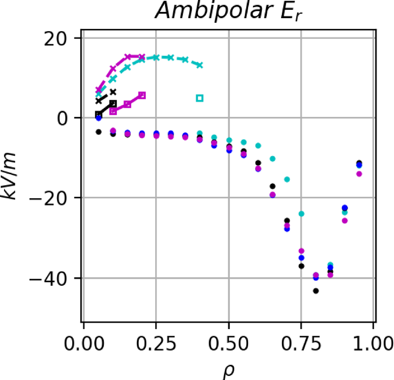
Figure 12. Ambipolar radial electric field solution $E_r$
for the cases shown in figure 10.
$E_r$
for the cases shown in figure 10. $\beta = 0.8\,\%$
(dark turquoise) is in the electron-root
$\beta = 0.8\,\%$
(dark turquoise) is in the electron-root $\rho \lt 0.3$
and in the ion-root otherwise. The target operating point,
$\rho \lt 0.3$
and in the ion-root otherwise. The target operating point, $\beta = 1.6\,\%$
(black) has only a small region near the axis that has multiple stable roots. At
$\beta = 1.6\,\%$
(black) has only a small region near the axis that has multiple stable roots. At $\beta = 2.4\,\%$
(blue), the electron-root solution vanishes entirely. At
$\beta = 2.4\,\%$
(blue), the electron-root solution vanishes entirely. At $\beta = 4.0\,\%$
, (magenta) the electron-root reappears as the only stable solution near the axis,
$\beta = 4.0\,\%$
, (magenta) the electron-root reappears as the only stable solution near the axis, $\rho \leqslant 0.1$
.
$\rho \leqslant 0.1$
.
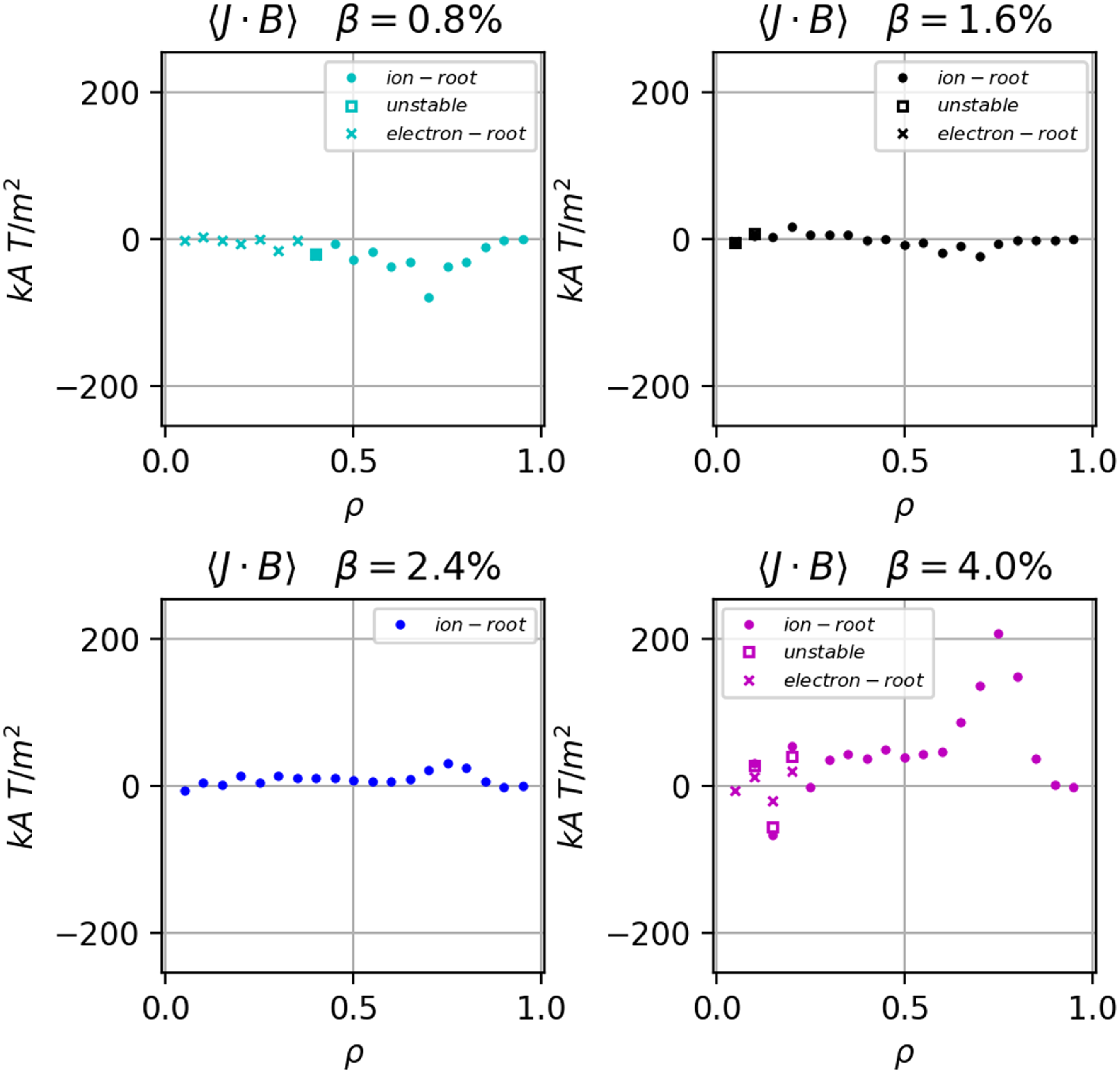
Figure 13. Radial profile of the bootstrap current $\langle J\cdot B \rangle$
for electron–proton plasmas for cases shown in figure 10. The net bootstrap current changes sign from low
$\langle J\cdot B \rangle$
for electron–proton plasmas for cases shown in figure 10. The net bootstrap current changes sign from low $\beta$
to high
$\beta$
to high $\beta$
, with almost no net current at
$\beta$
, with almost no net current at $\beta = 2.0\,\%$
(not shown). The difference in localised current densities between the electron- and ion-roots is small in these cases.
$\beta = 2.0\,\%$
(not shown). The difference in localised current densities between the electron- and ion-roots is small in these cases.
4.2. High-density test scenarios, bootstrap current, equilibrium limits and stability predictions
In the scenarios with $\beta$
above the target operating point, the net bootstrap current reduces to zero and then reverses direction shown in figure 13. The effect on the rotational transform profile is to reduce its value. While the
$\beta$
above the target operating point, the net bootstrap current reduces to zero and then reverses direction shown in figure 13. The effect on the rotational transform profile is to reduce its value. While the $n/m = 3/4$
is not a value that resonates with the equilibrium’s field periodicity (although
$n/m = 3/4$
is not a value that resonates with the equilibrium’s field periodicity (although $n/m = 12/16 = 0.75$
does), it could potentially play a role in stellarator symmetry breaking magnetic island formation, the stability of global MHD modes (discussed in § 4.3.3) and Alfvén eigenmodes (Carbajal et al. Reference Carbajal2025). Of course, in practice, the rational surface can be avoided by adding rotational transform through auxiliary coils if required. Fine control of the rotational transform has been demonstrated in W7-X (Andreeva et al. Reference Andreeva, Bräuer, Endler, Kisslinger and Igitkhanov2004).
$n/m = 12/16 = 0.75$
does), it could potentially play a role in stellarator symmetry breaking magnetic island formation, the stability of global MHD modes (discussed in § 4.3.3) and Alfvén eigenmodes (Carbajal et al. Reference Carbajal2025). Of course, in practice, the rational surface can be avoided by adding rotational transform through auxiliary coils if required. Fine control of the rotational transform has been demonstrated in W7-X (Andreeva et al. Reference Andreeva, Bräuer, Endler, Kisslinger and Igitkhanov2004).
HINT simulations for the scenarios at the the elevated $\beta = 4\,\%$
predict that a higher-order
$\beta = 4\,\%$
predict that a higher-order $m=11$
island appears near the periphery of the plasma, radially closer to the magnetic axis than the
$m=11$
island appears near the periphery of the plasma, radially closer to the magnetic axis than the ${\iota\kern-3.5pt\def\negativespace{}\mbox{-}\kern0.5pt}=0.80$
edge island resonance (see figure 14). Furthermore, the Shafranov shift of the magnetic axis differs by approximately 2 cm. At elevated levels of plasma pressure, the simulation predicts that the nested flux surfaces will break and an internal island will develop. However, other soft limits set by stability considerations may play a role before the plasmas were to reach a level of
${\iota\kern-3.5pt\def\negativespace{}\mbox{-}\kern0.5pt}=0.80$
edge island resonance (see figure 14). Furthermore, the Shafranov shift of the magnetic axis differs by approximately 2 cm. At elevated levels of plasma pressure, the simulation predicts that the nested flux surfaces will break and an internal island will develop. However, other soft limits set by stability considerations may play a role before the plasmas were to reach a level of $\beta \sim 4\,\%$
, as discussed in the next section. Nonetheless, these simulations indicate that the Infinity Two FPP configuration has robust magnetic surface integrity up to
$\beta \sim 4\,\%$
, as discussed in the next section. Nonetheless, these simulations indicate that the Infinity Two FPP configuration has robust magnetic surface integrity up to $\beta$
values well beyond that required for
$\beta$
values well beyond that required for $800\ \textrm{MW}$
DT fusion operation.
$800\ \textrm{MW}$
DT fusion operation.
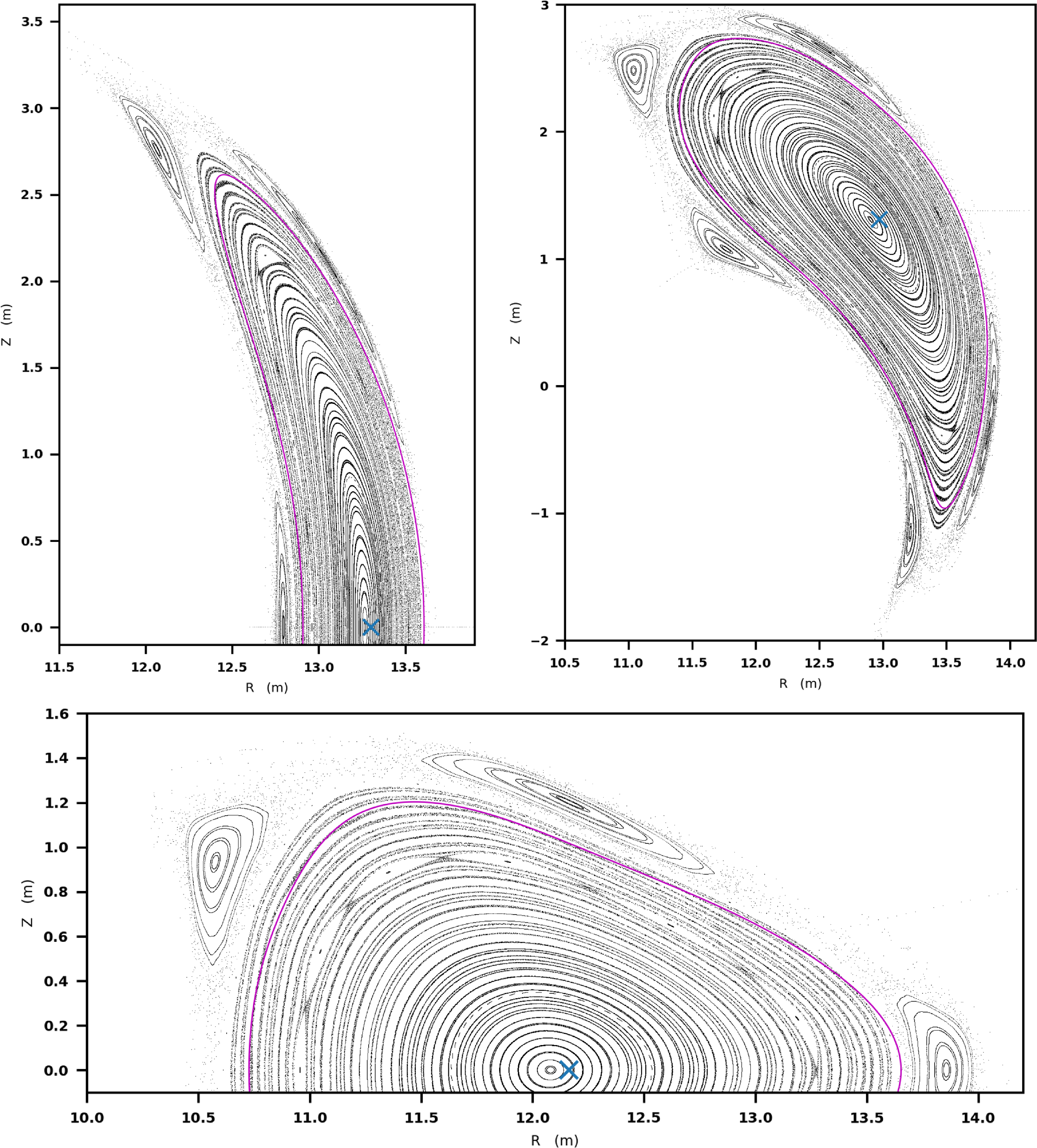
Figure 14. HINT results with elevated pressure at $2.5\times$
higher than the base operating point, with
$2.5\times$
higher than the base operating point, with $\beta \sim 4\,\%$
. One island forms in the periphery, with m = 11, and the edge becomes more stochastic compared with the operating point, figure 9.
$\beta \sim 4\,\%$
. One island forms in the periphery, with m = 11, and the edge becomes more stochastic compared with the operating point, figure 9.
4.3. Stability predictions
4.3.1. Mercier stability
The Mercier criterion can be expressed as (Bauer, Betancourt & Garabedian Reference Bauer, Betancourt and Garabedian1984; Carreras et al. Reference Carreras, Dominguez, Garcia, Lynch, Lyon, Cary, Hanson and Navarro1988)
 \begin{align} &D_{\rm Mercier} = D_S + D_W + D_I + D_G \geqslant 0. \end{align}
As shown in figure 15, Mercier stability is satisfied across the majority of the radial profiles, and the stability characteristics improve with increasing plasma pressure. The individual terms of (B.3) are plotted in figure 16. The shear of the transform is small in the core and steep near the edge. The profile of $D_S$
shows that regions close to zero shear have a destabilising influence, and the radial location and span vary with
$D_S$
shows that regions close to zero shear have a destabilising influence, and the radial location and span vary with $\beta$
. The edge is always stabilising. The profile of the magnetic well term (
$\beta$
. The edge is always stabilising. The profile of the magnetic well term ( $D_W$
) shows a stabilising effect that improves with
$D_W$
) shows a stabilising effect that improves with $\beta$
. The
$\beta$
. The $D_I$
-term, related to the net toroidal current, is destabilising at low
$D_I$
-term, related to the net toroidal current, is destabilising at low $\beta$
. With increasing pressure, the net bootstrap current decreases and the
$\beta$
. With increasing pressure, the net bootstrap current decreases and the $D_I$
-contribution becomes stabilising for part of the outer half of the plasma core,
$D_I$
-contribution becomes stabilising for part of the outer half of the plasma core, $0.5 \lt \rho \lt 0.8$
at
$0.5 \lt \rho \lt 0.8$
at $\beta \sim 1.6\,\%$
. It continues to become more stabilising with increasing pressure, even when the bootstrap current changes direction and increases in magnitude, except for the region near
$\beta \sim 1.6\,\%$
. It continues to become more stabilising with increasing pressure, even when the bootstrap current changes direction and increases in magnitude, except for the region near $\rho \sim 0.7$
, where the current density is the largest. The
$\rho \sim 0.7$
, where the current density is the largest. The $D_G$
term is destabilising, and its effect grows with
$D_G$
term is destabilising, and its effect grows with $\beta$
. Across most of the radius, the largest terms are
$\beta$
. Across most of the radius, the largest terms are $D_W$
and
$D_W$
and $D_G$
by 2–3 orders of magnitude. The terms are closer in magnitude near the edge, with
$D_G$
by 2–3 orders of magnitude. The terms are closer in magnitude near the edge, with $D_G$
being the largest at low-
$D_G$
being the largest at low- $\beta$
. The net stabilising effects of the terms related to the increased well depth, shear and current more than compensate for the destabilising effect of the geodesic curvature term, as seen in figure 16.
$\beta$
. The net stabilising effects of the terms related to the increased well depth, shear and current more than compensate for the destabilising effect of the geodesic curvature term, as seen in figure 16.
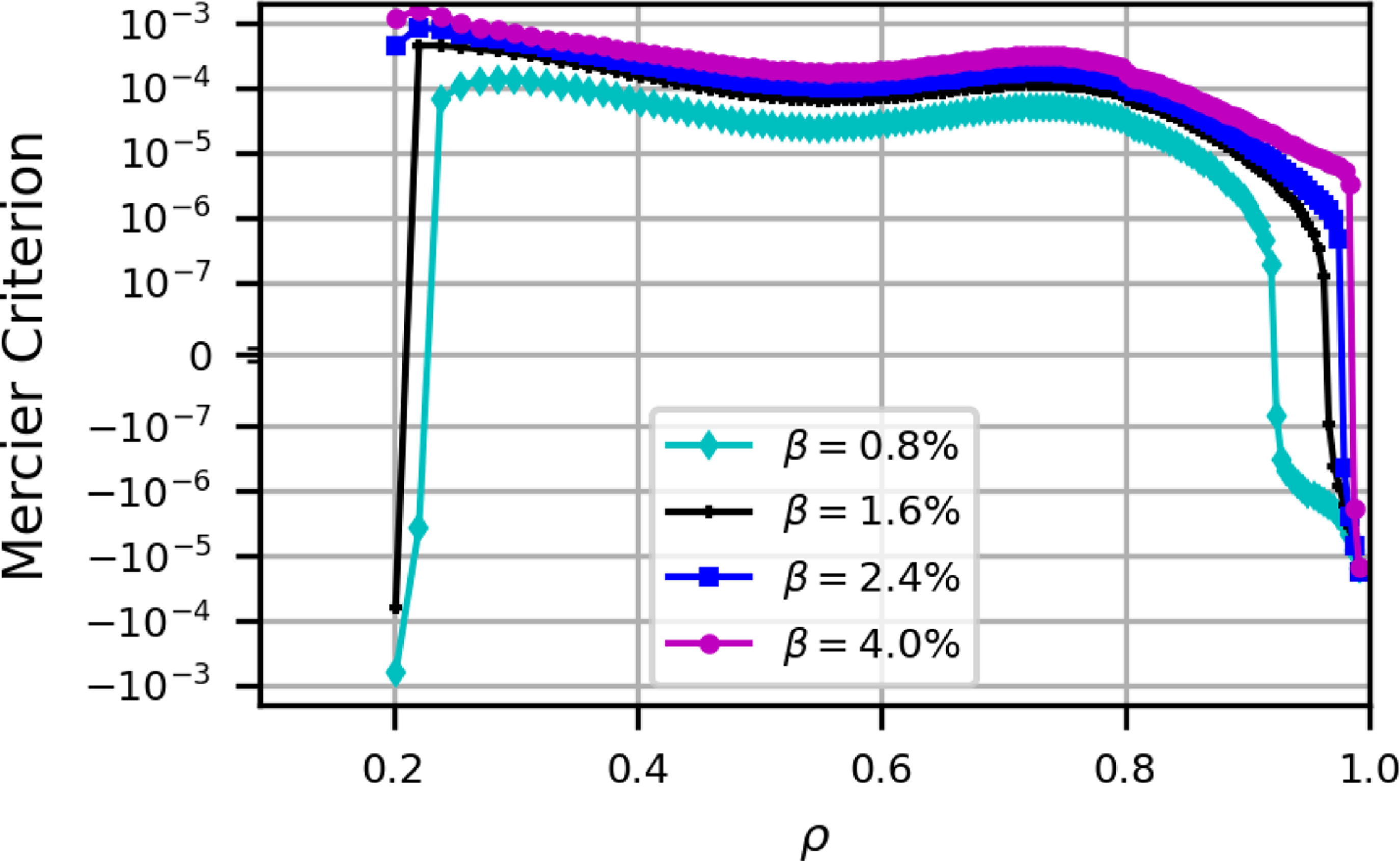
Figure 15. Radial profile of the Mercier criterion from $\beta =0.4\,\%$
to
$\beta =0.4\,\%$
to $\beta =4.0\,\%$
. The radial extent of the Mercier stable region increases with
$\beta =4.0\,\%$
. The radial extent of the Mercier stable region increases with $\beta$
, primarily due to the deepening magnetic well (see figure 16).
$\beta$
, primarily due to the deepening magnetic well (see figure 16).

Figure 16. Radial profiles of the components of the Mercier criterion from $\beta =0.4\,\%$
to
$\beta =0.4\,\%$
to $\beta =4.0\,\%$
. The largest terms are related to the magnetic well (
$\beta =4.0\,\%$
. The largest terms are related to the magnetic well ( $D_W$
, which is stabilising and improves with
$D_W$
, which is stabilising and improves with $\beta$
, see figure 11) and the geodesic curvature (
$\beta$
, see figure 11) and the geodesic curvature ( $D_G$
, which is destabilising and worsens with
$D_G$
, which is destabilising and worsens with $\beta$
). Where the shear of the transform is close to 0, the stabilising shear term, (
$\beta$
). Where the shear of the transform is close to 0, the stabilising shear term, ( $D_S$
) is also close to 0. The shear is always stabilising for
$D_S$
) is also close to 0. The shear is always stabilising for $\rho \gt 0.8$
. The current term (
$\rho \gt 0.8$
. The current term ( $D_I)$
tends to destabilise at the lowest
$D_I)$
tends to destabilise at the lowest $\beta$
, but at higher
$\beta$
, but at higher $\beta$
, it becomes a stabilising term, except for certain radially localised regions, e.g. close to
$\beta$
, it becomes a stabilising term, except for certain radially localised regions, e.g. close to $\rho \sim 0.7$
where the bootstrap current density is largest at
$\rho \sim 0.7$
where the bootstrap current density is largest at $\beta =4\,\%$
.
$\beta =4\,\%$
.
4.3.2. Infinite-N ballooning stability
Ballooning modes are localised along a field line in regions of unfavourable curvature (Freidberg Reference Freidberg2014). The modes are destabilised when the pressure gradient, $p'=(\textrm{d}p)/(\textrm{d}s)$
, is above some threshold. Stabilisation occurs through magnetic field-line bending (Hegna & Nakajima Reference Hegna and Nakajima1998).
$p'=(\textrm{d}p)/(\textrm{d}s)$
, is above some threshold. Stabilisation occurs through magnetic field-line bending (Hegna & Nakajima Reference Hegna and Nakajima1998).
For each of the equilibria described above, ballooning stability was evaluated with the COBRAVMEC code (Sanchez, Hirshman & Ware Reference Sanchez, Hirshman and Ware2000) and the Julia-based adaptation available in StellaratorOptimizationMetrics (Faber & Bader Reference Faber and Bader2024b). For the profiles in figure 1, the configuration is stable against ballooning modes up to $\beta \approx 2\,\%$
. The standard ballooning analysis considers only up to
$\beta \approx 2\,\%$
. The standard ballooning analysis considers only up to $k_w=10$
helical wells, which predicts stability in the region for
$k_w=10$
helical wells, which predicts stability in the region for $\rho \gt 0.9$
even though the Mercier criterion is strictly violated. If the analysis is extended to account for very long wavelengths,
$\rho \gt 0.9$
even though the Mercier criterion is strictly violated. If the analysis is extended to account for very long wavelengths, $k_w=300$
, the ballooning growth rate is positive, consistent with Mercier. Above that, regions that are ballooning unstable develop near
$k_w=300$
, the ballooning growth rate is positive, consistent with Mercier. Above that, regions that are ballooning unstable develop near $\rho \approx 0.7 {-} 0.8$
. This unstable region grows in radial extent and the growth rates increase with
$\rho \approx 0.7 {-} 0.8$
. This unstable region grows in radial extent and the growth rates increase with $\beta$
. In practice, however, this should not be viewed as a
$\beta$
. In practice, however, this should not be viewed as a $\beta$
-limit of the configuration. At high operating
$\beta$
-limit of the configuration. At high operating $\beta$
, kinetic ballooning modes emerge in the turbulent transport simulations which have the effect of lowering the gradients in the vicinity of the ideal ballooning stability boundary. The profiles of figure 1 were informed by the high-fidelity modelling of Guttenfelder et al. (Reference Guttenfelder2025). Further analysis in that same work develops a converged, self-consistent transport solution with profiles which have reduced pressure gradients in the edge region. If those profiles, shown in figure 9 of Guttenfelder et al. (Reference Guttenfelder2025), are used for the
$\beta$
, kinetic ballooning modes emerge in the turbulent transport simulations which have the effect of lowering the gradients in the vicinity of the ideal ballooning stability boundary. The profiles of figure 1 were informed by the high-fidelity modelling of Guttenfelder et al. (Reference Guttenfelder2025). Further analysis in that same work develops a converged, self-consistent transport solution with profiles which have reduced pressure gradients in the edge region. If those profiles, shown in figure 9 of Guttenfelder et al. (Reference Guttenfelder2025), are used for the $\beta$
scan instead of the model profiles of figure 1, the ideal ballooning onset occurs near
$\beta$
scan instead of the model profiles of figure 1, the ideal ballooning onset occurs near $\beta = 2.5\,\%$
. Indeed, the self-consistent transport modelling has the effect of shifting the location of the trouble spots to a slightly larger radial location,
$\beta = 2.5\,\%$
. Indeed, the self-consistent transport modelling has the effect of shifting the location of the trouble spots to a slightly larger radial location, $\rho \approx 0.75 {-} 0.85$
.
$\rho \approx 0.75 {-} 0.85$
.
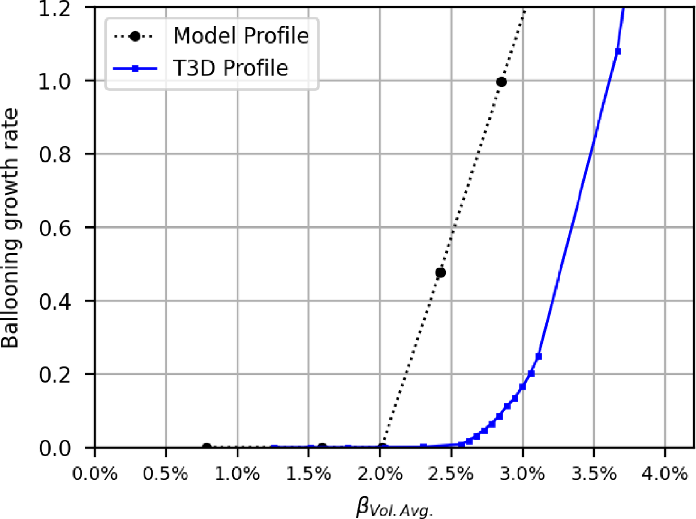
Figure 17. Peak growth rate for ballooning modes versus the plasma $\beta$
for three different profile shapes. Model profile, the profiles from figure 1 result in a conservative limit,
$\beta$
for three different profile shapes. Model profile, the profiles from figure 1 result in a conservative limit, $\beta \sim 2\,\%$
; T3D profile, scans with self-consistent profiles predict a higher limit,
$\beta \sim 2\,\%$
; T3D profile, scans with self-consistent profiles predict a higher limit, $\beta =2.5\,\%$
. The modified profiles result in reduced transport at the locations of strong ballooning drive.
$\beta =2.5\,\%$
. The modified profiles result in reduced transport at the locations of strong ballooning drive.
4.3.3. Finite-N global MHD stability
The ideal MHD stability of magnetically confined plasmas is described by a variational formulation of the linearised equations of motion coupled with the continuity equation, an equation of state that governs the pressure evolution, Maxwell’s equations that includes Ampère’s law, and Ohm’s law. This was formulated by Bernstein et al. (Reference Bernstein, Frieman, Kruskal and Kulsrud1958) and serves as the basis for the development of computer codes to investigate tokamaks, reversed field pinches, stellarators and other confinement systems. For stellarator configurations, the assumption has relied on MHD equilibrium states with nested magnetic flux surfaces, until quite recently. Recent work (Kumar et al. Reference Kumar2022) has demonstrated that a multi-region relaxed variational principle can be used to predict linear and ideal MHD stabilities using the stepped pressure equilibrium code (Hudson et al. Reference Hudson, Dewar, Dennis, Hole, McGann, von Nessi and Lazerson2012). Here, however, we use the nested flux surface model.
The Infinity Two FPP configuration considered here is stable to global ideal MHD modes at low and intermediate toroidal mode numbers $\texttt {n}$
at
$\texttt {n}$
at $\beta = 1.6 \,\%$
. Figure 18 shows that the configuration becomes unstable to low
$\beta = 1.6 \,\%$
. Figure 18 shows that the configuration becomes unstable to low $n \lt 15$
modes only when
$n \lt 15$
modes only when $\beta$
exceeds
$\beta$
exceeds $3.5\ \%$
. From the possible set of toroidal resonances, the most unstable low-
$3.5\ \%$
. From the possible set of toroidal resonances, the most unstable low- ${n}$
mode we have computed at
${n}$
mode we have computed at $\beta =3.7\ \%$
corresponds to that of the
$\beta =3.7\ \%$
corresponds to that of the $n=1$
mode family (
$n=1$
mode family ( $n=\pm \, 1,\pm \, 3,\ldots \pm 11,\ldots$
) in which the
$n=\pm \, 1,\pm \, 3,\ldots \pm 11,\ldots$
) in which the $m/n=16/11$
component is dominant (a brief description of the resolution and mode families is in Appendix F).
$m/n=16/11$
component is dominant (a brief description of the resolution and mode families is in Appendix F).
We display on the right of figure 18 the profiles of the leading Fourier amplitudes corresponding to the perturbed radial magnetic field $\delta \vec {B}\cdot \nabla s\equiv \delta B^s$
for the N = 1 family. The particular normalisation chosen in this plot (
$\delta \vec {B}\cdot \nabla s\equiv \delta B^s$
for the N = 1 family. The particular normalisation chosen in this plot ( $\sqrt {g}\delta B^s/\psi _t'(s)$
) is in dimensionless units to facilitate cross-configuration and cross-device comparisons. The radial magnetic field structure impact on phenomena such as fast ion transport would constitute a critical issue at the elevated
$\sqrt {g}\delta B^s/\psi _t'(s)$
) is in dimensionless units to facilitate cross-configuration and cross-device comparisons. The radial magnetic field structure impact on phenomena such as fast ion transport would constitute a critical issue at the elevated $\beta$
, but at the target operating point, the problem does not exist. The bottom row displays the eigenvalues for the three distinct mode families as a function of
$\beta$
, but at the target operating point, the problem does not exist. The bottom row displays the eigenvalues for the three distinct mode families as a function of $\beta$
for low toroidal mode numbers
$\beta$
for low toroidal mode numbers $n\lt 15$
. The left plot uses a linear scale and the right plot uses a semi-log scale for the y-axis. Stable modes at the continuum are always near the marginal point
$n\lt 15$
. The left plot uses a linear scale and the right plot uses a semi-log scale for the y-axis. Stable modes at the continuum are always near the marginal point $\lambda =0$
. Hence, the logarithm of
$\lambda =0$
. Hence, the logarithm of $\texttt {ln}(|(\lambda |)$
will be very negative. Only the significantly unstable modes will be large in this plot. The dashed line indicates the value of
$\texttt {ln}(|(\lambda |)$
will be very negative. Only the significantly unstable modes will be large in this plot. The dashed line indicates the value of $\lambda \texttt { = -0.001}$
. So any value of
$\lambda \texttt { = -0.001}$
. So any value of $\texttt {ln}(|(\lambda |)$
less than this corresponds either to a stable mode or a weakly unstable mode. Very localised unstable mode structures near the core of the plasma can become destabilised. We consider these modes spurious as a result of the poor reconstruction of the derivative of the equilibrium pressure in the vicinity of the magnetic axis.
$\texttt {ln}(|(\lambda |)$
less than this corresponds either to a stable mode or a weakly unstable mode. Very localised unstable mode structures near the core of the plasma can become destabilised. We consider these modes spurious as a result of the poor reconstruction of the derivative of the equilibrium pressure in the vicinity of the magnetic axis.
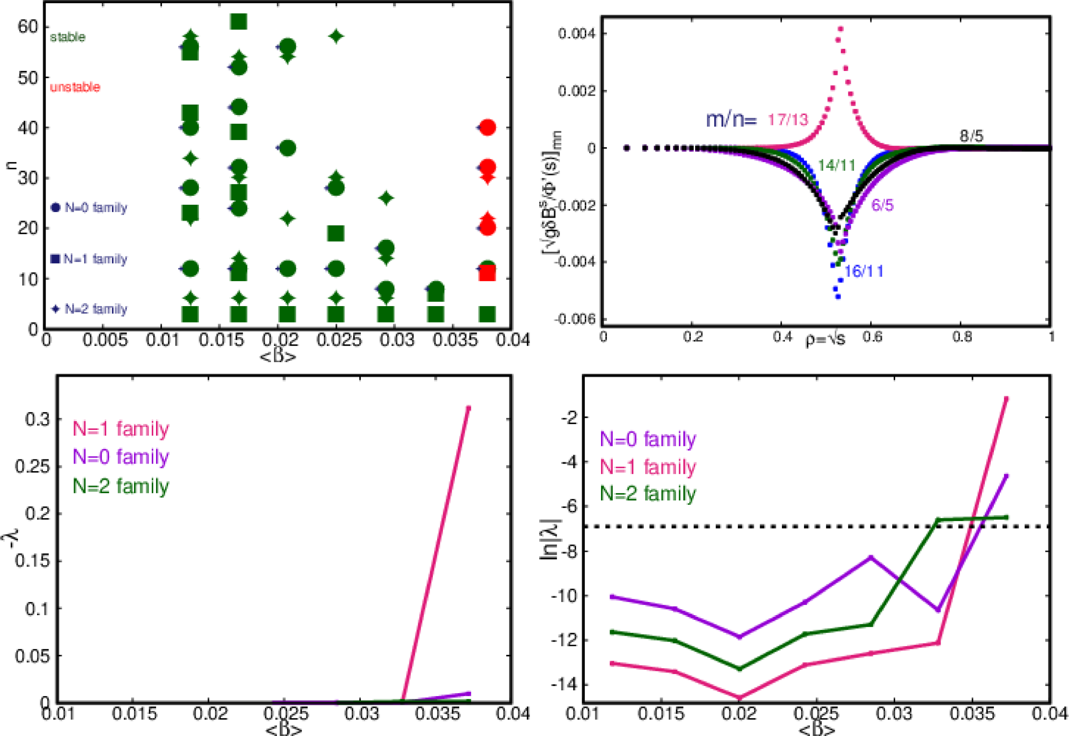
Figure 18. Global stability. Top left, the circles indicate modes of the stellarator symmetry breaking n = 0 family, squares represent periodicity breaking modes of the n = 1 family and diamonds correspond to modes of the n = 2 family (they impose two-fold periodicity around the torus). The symbols in green identify stable modes and the red symbols represent more global unstable modes that appear at high $\beta \gt 3.5\,\%$
. Top right, radial profiles of the five leading amplitudes of
$\beta \gt 3.5\,\%$
. Top right, radial profiles of the five leading amplitudes of $\sqrt {g}\delta B^s/\varPhi '(s)$
at
$\sqrt {g}\delta B^s/\varPhi '(s)$
at $\beta =3.7\,\%$
for the unstable mode where the
$\beta =3.7\,\%$
for the unstable mode where the ${m/n}=16/11$
component is dominant. The bottom row displays the eigenvalues for the three distinct mode families as a function of
${m/n}=16/11$
component is dominant. The bottom row displays the eigenvalues for the three distinct mode families as a function of $\beta$
for low toroidal mode numbers
$\beta$
for low toroidal mode numbers ${n}\lt 15$
. Left, linear scale. Right, semi-log scale.
${n}\lt 15$
. Left, linear scale. Right, semi-log scale.
5. Summary and discussion
The Infinity Two FPP configuration presented in this work includes a candidate coil set and a set of plasma profiles that are expected to reach fusion conditions. The operating density was scaled as a proxy to study low- to high- $\beta$
operating scenarios. Poincaré maps constructed with line-following of the vacuum fields show that good flux surfaces are present. HINT evaluations at the operating point, along with subsequent post-processing line-following, demonstrate that good flux surfaces are also predicted from vacuum up to the finite
$\beta$
operating scenarios. Poincaré maps constructed with line-following of the vacuum fields show that good flux surfaces are present. HINT evaluations at the operating point, along with subsequent post-processing line-following, demonstrate that good flux surfaces are also predicted from vacuum up to the finite $\beta$
operating point. The edge topology changes only slightly within the target operating range. The configuration is robust against ballooning modes, is stable against low-n and high-n global MHD modes, and has a stabilising magnetic well, which deepens with
$\beta$
operating point. The edge topology changes only slightly within the target operating range. The configuration is robust against ballooning modes, is stable against low-n and high-n global MHD modes, and has a stabilising magnetic well, which deepens with $\beta$
, across the entire profile from vacuum up to its operating point. This indicates that a clear path from vacuum to the operating point exists in terms of controlling the edge island structure for divertor operations. It is expected to achieve stationary finite-
$\beta$
, across the entire profile from vacuum up to its operating point. This indicates that a clear path from vacuum to the operating point exists in terms of controlling the edge island structure for divertor operations. It is expected to achieve stationary finite- $\beta$
conditions without disruptive activity and with minimal need to control external coil currents for island position control.
$\beta$
conditions without disruptive activity and with minimal need to control external coil currents for island position control.
At elevated levels of $\beta$
above the target operating point, the depth of the magnetic well continues to increase. Ballooning modes with the profiles presented here are stable up to
$\beta$
above the target operating point, the depth of the magnetic well continues to increase. Ballooning modes with the profiles presented here are stable up to $\beta =2.0 \,\%$
. Above that, regions of bad curvature near the
$\beta =2.0 \,\%$
. Above that, regions of bad curvature near the $\rho \approx 0.7 {-} 0.8$
radius appear to go unstable first. However, that prediction is a conservative one. The self-consistent transport modelling (Guttenfelder et al. Reference Guttenfelder2025) predicted a reduction of the transport to alleviate the strong ballooning drive near
$\rho \approx 0.7 {-} 0.8$
radius appear to go unstable first. However, that prediction is a conservative one. The self-consistent transport modelling (Guttenfelder et al. Reference Guttenfelder2025) predicted a reduction of the transport to alleviate the strong ballooning drive near $\rho \sim 0.7$
. Evaluations with the self-consistent profiles predicted an ideal ballooning limit of
$\rho \sim 0.7$
. Evaluations with the self-consistent profiles predicted an ideal ballooning limit of $\beta = 2.5\,\%$
with the location of the most unstable ballooning modes at the outer radii of
$\beta = 2.5\,\%$
with the location of the most unstable ballooning modes at the outer radii of $0.75 \leqslant \rho \leqslant 0.85$
. Global MHD modes exhibit regions of very localised instability near the core at pressures just above the
$0.75 \leqslant \rho \leqslant 0.85$
. Global MHD modes exhibit regions of very localised instability near the core at pressures just above the $\beta =1.6\,\%$
operating point, but these are considered spurious. Global low-n modes are stable up to
$\beta =1.6\,\%$
operating point, but these are considered spurious. Global low-n modes are stable up to $\beta =3.2\,\%$
. Large global instabilities of the
N
= 1 family are expected to appear at the highest values of pressure explored in this work.
$\beta =3.2\,\%$
. Large global instabilities of the
N
= 1 family are expected to appear at the highest values of pressure explored in this work.
Several important items are left for future work. Manufacturing, assembly and placement errors of the field coils can result in magnetic field errors that can degrade the quality of flux surfaces, change the magnetic spectrum, alter stability limits, affect the neoclassical bootstrap current and negatively affect transport properties. Anticipating and including the uncertainties related to the coil set as-built will rely on the MHD models as part of the analysis workflow. Performing full-torus evaluations with HINT will be critical to confirm that no symmetry-breaking errors are present. Nonlinear simulations with stellarator geometries will also provide confidence of the stability of the operating point (Schlutt et al. Reference Schlutt, Hegna, Sovinec, Held and Kruger2013; Sovinec et al. Reference Sovinec, Cornille, Gupta, Ingram, McCollam, Patil, Sainterme and Tillinghast2022; Ramasamy et al. Reference Ramasamy, Aleynikova, Nikulsin, Hindenlang, Holod, Strumberger and Hoelzl2024; Wright & Ferraro Reference Wright and Ferraro2024). The sensitivity of the operating point to uncertainties in the profiles will be explored in the future. While the Shafranov shift is projected to be proportional to $\beta$
, the bootstrap current can be quite sensitive to changes in the profiles. However, like other QI configurations, this device exhibits the feature of having low to no bootstrap and small Pfirsch–Schlüter currents, and is predicted to experience small distortions and motions of the plasma column as the plasma pressure increases. Plasma flows are neglected or artificially damped in the both VMEC or HINT. The quasi-isodynamic configuration does not have a preferred direction of symmetry and plasma flows, if present, are expected to be small. Large internal islands are not present and the HINT simulations predicts robust flux surfaces up to the operating point. Regardless, if islands were to develop, such as in the simulated
$\beta$
, the bootstrap current can be quite sensitive to changes in the profiles. However, like other QI configurations, this device exhibits the feature of having low to no bootstrap and small Pfirsch–Schlüter currents, and is predicted to experience small distortions and motions of the plasma column as the plasma pressure increases. Plasma flows are neglected or artificially damped in the both VMEC or HINT. The quasi-isodynamic configuration does not have a preferred direction of symmetry and plasma flows, if present, are expected to be small. Large internal islands are not present and the HINT simulations predicts robust flux surfaces up to the operating point. Regardless, if islands were to develop, such as in the simulated $\beta =4.0\,\%$
case, even small residual plasma flows may be sufficient to ‘heal’ them (Narushima et al. Reference Narushima, Watanabe, Sakakibara, Narihara, Yamada, Suzuki, Ohdachi, Ohyabu, Yamada and Nakamura2008; Hegna Reference Hegna2011). No extra control is required for the classical divertor design proposed by Bader et al. (Reference Bader2025), but the local island backside divertor would likely require actively controlled external island-control coils similar to the control and/or planar coils of W7-X (Risse et al. Reference Risse, Rummel, Bosch, Bykov, Carls, Füllenbach, Mönnich, Nagel and Schneider2018) for fine control of the island position and shape.
$\beta =4.0\,\%$
case, even small residual plasma flows may be sufficient to ‘heal’ them (Narushima et al. Reference Narushima, Watanabe, Sakakibara, Narihara, Yamada, Suzuki, Ohdachi, Ohyabu, Yamada and Nakamura2008; Hegna Reference Hegna2011). No extra control is required for the classical divertor design proposed by Bader et al. (Reference Bader2025), but the local island backside divertor would likely require actively controlled external island-control coils similar to the control and/or planar coils of W7-X (Risse et al. Reference Risse, Rummel, Bosch, Bykov, Carls, Füllenbach, Mönnich, Nagel and Schneider2018) for fine control of the island position and shape.
Acknowledgements
We gratefully acknowledge the use of the computational resources managed and supported by Princeton Research Computing, a consortium of groups including the Princeton Institute for Computational Science and Engineering (PICSciE) and the Office of Information Technology’s High Performance Computing Center and Visualization Laboratory at Princeton University.
Editor Per Helander thanks the referees for their advice in evaluating this article.
Funding
We gratefully acknowledge the use of National Energy Research Scientific Computing Center (NERSC) resources, a Department of Energy Office of Science User Facility using NERSC award FES-ERCAP27470.
Declaration of interests
The work of M.L. and W.D. was performed as consultants and was not part of the employees’ responsibilities to the University of Maryland. The work of J.V. was performed as a consultant and was not part of the employee’s responsibilities at the University of Texas.
Appendix A. Magnetic well
In a toroidal geometry, the specific volume, $U$
, is a flux-surface quantity defined as the change in volume with respect to increasing enclosed toroidal flux
$U$
, is a flux-surface quantity defined as the change in volume with respect to increasing enclosed toroidal flux $\psi _t$
(Miyamoto Reference Miyamoto1987):
$\psi _t$
(Miyamoto Reference Miyamoto1987):
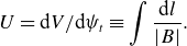 \begin{align} U &= \textrm{d}V / \textrm{d}\psi _t \equiv \int \frac {\textrm{d}l}{|B|}. \end{align}
The integral is evaluated along a magnetic field line on the flux surface and $|B|$
is the magnitude of the magnetic field along the field line. When the derivative of the specific volume is positive,
$|B|$
is the magnitude of the magnetic field along the field line. When the derivative of the specific volume is positive, $\textrm{d}U/\textrm{d}\psi _t\gt 0$
, a destabilising magnetic hill is present. A negative derivative,
$\textrm{d}U/\textrm{d}\psi _t\gt 0$
, a destabilising magnetic hill is present. A negative derivative, $\textrm{d}U/\textrm{d}\psi _t\lt 0$
, indicates a magnetic well. The depth of the magnetic well as a function of radius is defined by (Wakatani Reference Wakatani1998)
$\textrm{d}U/\textrm{d}\psi _t\lt 0$
, indicates a magnetic well. The depth of the magnetic well as a function of radius is defined by (Wakatani Reference Wakatani1998)
 \begin{align} -\frac {\Delta U}{U} = \frac {U_\textrm{axis} - U(\rho )}{U_{\rm axis}}. \end{align}
A positive gradient of the well depth indicates a region with a magnetic well and a negative gradient indicates a region with a magnetic hill.
Appendix B. VMEC
The Variational Moments Equilibrium Code (VMEC) solves the ideal 3-D MHD equilibrium under the assumption of closed, nested flux surfaces. The model assumes a static isotropic plasma with no fluid flows is sought that satisfies:
 \begin{align} &\vec {F} = \vec {J} \times \vec {B}-\nabla p = 0 ,\end{align}
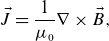 \begin{align} &\vec {J} = \frac {1}{\mu _0}\nabla \times \vec {B}, \end{align}
 \begin{align} &\nabla \cdot \vec {B} = 0, \end{align}
 \begin{align} &p = p(s),\\[6pt]\nonumber\end{align}
where $\vec {J}$
is the plasma current density,
$\vec {J}$
is the plasma current density, $\vec {B}$
is the total magnetic field,
$\vec {B}$
is the total magnetic field, $p$
is the plasma pressure and
$p$
is the plasma pressure and $\mu _0$
is the permeability of free space. An inverse coordinate representation is employed:
$\mu _0$
is the permeability of free space. An inverse coordinate representation is employed: $\vec {X} = \vec {X}\left (s, \theta , \zeta \right )$
, where
$\vec {X} = \vec {X}\left (s, \theta , \zeta \right )$
, where $s$
is the flux surface label, and
$s$
is the flux surface label, and $\theta$
and
$\theta$
and $\zeta$
are poloidal and toroidal angles, respectively. The default radial grid is uniform in
$\zeta$
are poloidal and toroidal angles, respectively. The default radial grid is uniform in $s=\psi _t/\psi _{t,LCFS}$
, where
$s=\psi _t/\psi _{t,LCFS}$
, where $\psi _t$
is the enclosed toroidal flux and
$\psi _t$
is the enclosed toroidal flux and $\textrm{LCFS}$
stands for last closed flux surface. The coordinates
$\textrm{LCFS}$
stands for last closed flux surface. The coordinates $R$
and
$R$
and $Z$
of the surfaces are expanded in two-dimensional (2-D) Fourier series in poloidal angle
$Z$
of the surfaces are expanded in two-dimensional (2-D) Fourier series in poloidal angle $\theta$
and toroidal angle
$\theta$
and toroidal angle $\zeta$
. In VMEC,
$\zeta$
. In VMEC, $\zeta$
is equal to the laboratory toroidal angle
$\zeta$
is equal to the laboratory toroidal angle $\phi$
. Islands cannot be described in the nested flux surface model assumed by VMEC. The boundary can either be a fixed constraint or an initial guess. In the first case, the boundary geometry is taken as an input to the computation, and the boundary condition
$\phi$
. Islands cannot be described in the nested flux surface model assumed by VMEC. The boundary can either be a fixed constraint or an initial guess. In the first case, the boundary geometry is taken as an input to the computation, and the boundary condition $\vec {B}\cdot \vec {n}=0$
is imposed there: the computational boundary acts as a perfectly conducting wall and surface currents flowing in that perfectly conducting wall contribute to holding the plasma in force balance inside the boundary. This describes the fixed-boundary VMEC calculations. In contrast, in free-boundary VMEC calculations, the plasma is held in force balance by external coils, and the location of the plasma boundary is computed self-consistently together with the plasma equilibrium. Specifically, the equilibrium is considered to be achieved when the residual force,
$\vec {B}\cdot \vec {n}=0$
is imposed there: the computational boundary acts as a perfectly conducting wall and surface currents flowing in that perfectly conducting wall contribute to holding the plasma in force balance inside the boundary. This describes the fixed-boundary VMEC calculations. In contrast, in free-boundary VMEC calculations, the plasma is held in force balance by external coils, and the location of the plasma boundary is computed self-consistently together with the plasma equilibrium. Specifically, the equilibrium is considered to be achieved when the residual force, $\vec {F}$
, in (B.1a
), is satisfied everywhere inside the plasma, and when the jump of the sum of the plasma pressure and the magnetic pressure across the plasma boundary is zero (to within some numerical accuracy) (Hirshman et al. Reference Hirshman1986).
$\vec {F}$
, in (B.1a
), is satisfied everywhere inside the plasma, and when the jump of the sum of the plasma pressure and the magnetic pressure across the plasma boundary is zero (to within some numerical accuracy) (Hirshman et al. Reference Hirshman1986).
For the VMEC evaluations listed in table 3, the number of poloidal modes (MPOL), the maximum toroidal mode number (NTOR), the number of radial surfaces and the desired residual force-balance of the VMEC solution are shown in table 4. Using fewer than 12 poloidal harmonics leads to inaccurate estimates of the rotational transform near the magnetic axis, and using more than 14 harmonics prohibits reliable VMEC convergence. The number of surfaces in the computations grid (NS) can be increased at the cost of minimal achievable FTOL and increased computational runtime.
Table 4. Fourier spectrum, radial grid and residual force balance parameters for the VMEC vacuum and finite- $\beta$
evaluations in this work.
$\beta$
evaluations in this work.
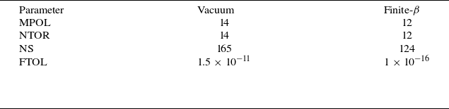
B.1 Mercier
The Mercier criterion (Mercier Reference Mercier1962) can be expressed as (Bauer et al. Reference Bauer, Betancourt and Garabedian1984; Carreras et al. Reference Carreras, Dominguez, Garcia, Lynch, Lyon, Cary, Hanson and Navarro1988)
 \begin{align} &D_{\rm Mercier} = D_S + D_W + D_I + D_G \geqslant 0. \end{align}
The individual terms are the stabilising ( $\gt 0$
) or destabilising (
$\gt 0$
) or destabilising ( $\lt 0$
) contributions of the shear (
$\lt 0$
) contributions of the shear ( $D_S$
), magnetic well (
$D_S$
), magnetic well ( $D_W$
), current (
$D_W$
), current ( $D_I$
), and geodesic curvature (
$D_I$
), and geodesic curvature ( $D_G$
). These are expressed as
$D_G$
). These are expressed as
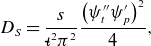 \begin{align} &D_S = \frac {s}{{\iota\kern-3.5pt\def\negativespace{}\mbox{-}\kern0.5pt}^2\pi ^2}\frac {\left (\psi _t''\psi _p'\right )^2}{4}, \end{align}
 \begin{align} &D_W =\frac {s}{{\iota\kern-3.5pt\def\negativespace{}\mbox{-}\kern0.5pt}^2\pi ^2}\int \int {\sqrt {g} \textrm{d}\theta \textrm{d}\zeta \frac {B^2}{g^{\rm ss}}\frac {\textrm{d}p}{\textrm{d}s}\left (V''-\frac {\textrm{d}p}{\textrm{d}s}\int \int {\sqrt {g}\frac {\textrm{d}\theta\textrm{d}\zeta }{B^2}} \right )} ,\end{align}
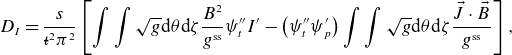 \begin{align} &D_I =\frac {s}{{\iota\kern-3.5pt\def\negativespace{}\mbox{-}\kern0.5pt}^2\pi ^2}\left [\int \int {\sqrt {g} \textrm{d}\theta \textrm{d}\zeta \frac {B^2}{g^{\rm ss}}\psi _t''I'} -\left (\psi _t''\psi _p'\right )\int \int {\sqrt {g} \textrm{d}\theta \textrm{d}\zeta \frac {\vec {J}\cdot \vec {B}}{g^{\rm ss}}}\right ], \end{align}
 \begin{align} &D_G =\frac {s}{{\iota\kern-3.5pt\def\negativespace{}\mbox{-}\kern0.5pt}^2\pi ^2}\left [\!\left (\int\!\!\int\! {\sqrt {g} \textrm{d}\theta \textrm{d}\zeta \frac {\vec {J}\cdot \vec {B}}{g^{\rm ss}} } \right )^2\!-\!\left (\!\int\!\!\int\! {\sqrt {g} \textrm{d}\theta \textrm{d}\zeta \frac {\left (\vec {J}\cdot \vec {B} \right )^2}{g^{\rm ss}B^2}} \right )\!\left (\int\!\!\int\! {\sqrt {g} \textrm{d}\theta \textrm{d}\zeta \frac {B^2}{g^{\rm ss}}} \right )\!\right]\!. \\[8pt] \nonumber \end{align}
Here, the Jacobian is $\sqrt {g} = 1/\nabla s\cdot \nabla \theta \times \nabla \zeta$
,
$\sqrt {g} = 1/\nabla s\cdot \nabla \theta \times \nabla \zeta$
, $g^{\rm ss}$
is the metric element
$g^{\rm ss}$
is the metric element $g^{\rm ss} = |\nabla s|^2$
and
$g^{\rm ss} = |\nabla s|^2$
and $V''=\textrm{d}V/\textrm{d}s$
. The domain of integration is over the entire flux surface,
$V''=\textrm{d}V/\textrm{d}s$
. The domain of integration is over the entire flux surface, $\theta \in [0,2\pi ], \zeta \in [0,2\pi ]$
. The terms of the Mercier criterion are evaluated by VMEC in the post-processing stage.
$\theta \in [0,2\pi ], \zeta \in [0,2\pi ]$
. The terms of the Mercier criterion are evaluated by VMEC in the post-processing stage.
Appendix C. HINT
HINT is a nonlinear 3-D MHD initial-value equilibrium code that employs a two-step relaxation method based on the dynamic equations of the magnetic field and pressure projected on an Eulerian grid (fixed in space). This grid selection allows HINT to represent islands and regions with stochastic magnetic field lines. The goal of using HINT is two-fold: (i) to provide a more accurate magnetic field in the region of the edge islands and (ii) to provide an indication of flux surface break-up in the plasma core at finite $\beta$
.
$\beta$
.
The HINT simulation is an iterative two-step process. The first step is a relaxation of the plasma pressure profile to satisfy the condition $\vec {B}\cdot \nabla p = 0$
. While
$\vec {B}\cdot \nabla p = 0$
. While $\vec {B}$
is held fixed, the plasma pressure at each grid point is updated for iteration
$\vec {B}$
is held fixed, the plasma pressure at each grid point is updated for iteration $i+1$
according to
$i+1$
according to
 \begin{align} &p^{i+1}=\bar{p} = \frac {\int _{-L_\textrm{max}}^{L_\textrm{max}} \mathcal {F} p^i \dfrac {\textrm{d}l}{B}}{\int _{-L_\textrm{max}}^{L_\textrm{max}}\dfrac {\textrm{d}l}{B}}, \end{align}
 \begin{align} &\mathcal {F} = \begin{cases} 1 & \text {for }L_C \geqslant L_\textrm{max},\\ 0 & \text {for }L_C \lt L_\textrm{max}, \end{cases}\\[6pt]\nonumber \end{align}
where $L_\textrm{max}$
, prescribed by the user, is the maximum length along a magnetic field line followed from each grid point in each toroidal direction (set to
$L_\textrm{max}$
, prescribed by the user, is the maximum length along a magnetic field line followed from each grid point in each toroidal direction (set to $10\ \textrm{m}$
here);
$10\ \textrm{m}$
here); $L_C$
is the connection length for each magnetic field line starting at each grid point. For open (closed) field lines,
$L_C$
is the connection length for each magnetic field line starting at each grid point. For open (closed) field lines, $L_C$
is finite (infinite). If the connection length is shorter than
$L_C$
is finite (infinite). If the connection length is shorter than $L_\textrm{max}$
, the averaged plasma pressure for that grid point is set to 0.
$L_\textrm{max}$
, the averaged plasma pressure for that grid point is set to 0.
The second step is a relaxation process of the magnetic field due to plasma currents, $\vec {B}_1$
, for fixed
$\vec {B}_1$
, for fixed $p$
. The artificial dissipative equations are
$p$
. The artificial dissipative equations are
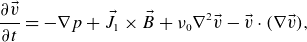 \begin{align} \frac {\partial \vec {v}}{\partial t} &= -\nabla p + \vec {J}_1 \times \vec {B}+\nu _0\nabla ^2\vec {v}-\vec {v}\cdot (\nabla \vec {v}), \end{align}
 \begin{align} \frac {\partial \vec {B}_1}{\partial t} &= \nabla \times (\vec {v}\times \vec {B} - \eta ( \vec {J} - \vec {J}_\textrm{net} ) ) + \kappa _{\textrm{div}B}\nabla (\nabla \cdot \vec {B}_1),\end{align}
 \begin{align} \vec {J}_1 &= \nabla \times \vec {B}_1,\\[6pt]\nonumber \end{align}
where $\vec {B}$
is the total magnetic field due to coil currents and plasma current. The fluid velocity is given by
$\vec {B}$
is the total magnetic field due to coil currents and plasma current. The fluid velocity is given by $\vec {v}$
. Here,
$\vec {v}$
. Here, $\eta$
is an electrical resistivity parameter;
$\eta$
is an electrical resistivity parameter; $\nu _0$
is the viscosity. To help accelerate convergence, these two terms are set artificially high and the mass density is normalised to 1. The
$\nu _0$
is the viscosity. To help accelerate convergence, these two terms are set artificially high and the mass density is normalised to 1. The $\kappa _{\textrm{div}B}$
-term provides numerical stabilisation to remove contributions arising from
$\kappa _{\textrm{div}B}$
-term provides numerical stabilisation to remove contributions arising from $\nabla \cdot \vec {B}_1 \ne 0$
on the computational grid. Additionally,
$\nabla \cdot \vec {B}_1 \ne 0$
on the computational grid. Additionally, $\vec {J}_{\rm net}$
is the net toroidal current defined as
$\vec {J}_{\rm net}$
is the net toroidal current defined as
 \begin{align} \vec {J}_\textrm{net} &= \vec {B}\frac {\langle \vec {J}\cdot \vec {B} \rangle }{B^2} .\end{align}
In the expression above, $\langle \mathcal {L}\rangle$
indicates a flux-surface average of the quantity
$\langle \mathcal {L}\rangle$
indicates a flux-surface average of the quantity $\mathcal {L}$
. HINT uses the constant pressure surfaces as a proxy for the flux surfaces. The volume average of
$\mathcal {L}$
. HINT uses the constant pressure surfaces as a proxy for the flux surfaces. The volume average of $(\nabla p - \vec {J}\times \vec {B}) ^2$
, and the quantities
$(\nabla p - \vec {J}\times \vec {B}) ^2$
, and the quantities $|\delta \vec {v}/\delta t|^2$
and
$|\delta \vec {v}/\delta t|^2$
and $|\delta \vec {B}/\delta t|^2$
are monitored as measures of convergence. A typical history of these quantities is shown in figure 19. The spikes in the early stages (
$|\delta \vec {B}/\delta t|^2$
are monitored as measures of convergence. A typical history of these quantities is shown in figure 19. The spikes in the early stages ( $t\lt 5$
) correspond to the pressure profile being applied in increasing steps, and the later spikes at
$t\lt 5$
) correspond to the pressure profile being applied in increasing steps, and the later spikes at $t=20,40,60$
correspond to the points in the simulation when HINT resets the pressure profile distribution on the computational grid. The connection length of the field lines, the rotational transform and fractal dimension were monitored for indications of the formation of islands and stochastic regions.
$t=20,40,60$
correspond to the points in the simulation when HINT resets the pressure profile distribution on the computational grid. The connection length of the field lines, the rotational transform and fractal dimension were monitored for indications of the formation of islands and stochastic regions.
Figure 19. Time history of the convergence properties of the HINT simulation.
C.1 Parameter settings
The HINT simulations in this work were performed on a computational mesh that spans a single field period. The number of grid points were 256 × 256 × 256 in the radial × vertical × toroidal direction, respectively. The results of the simulations do not change significantly if the resolution is reduced to 128 × 128 × 128, although some fidelity in the post-processed Poincaré maps is lost in the region around the edge island chain. A mesh size of 64 × 64 × 64 was unreliable for HINT simulations. The simulations were evaluated for a total of 80 iterations of steps ‘A’ and ‘B’. Full-torus simulations are planned for the future to explore for the effects of symmetry-breaking errors.
C.2 Identifying the last closed flux surface of the finite- $\beta$
solution
$\beta$
solution

The last closed flux surface of each of the finite-beta solutions was estimated by inspecting the Poincaré maps generated with the magnetic field of the HINT simulations. The HINT simulations included the first wall model presented by Bader et al. (Reference Bader2025), but did not include either of the divertor models presented there. Detailed transport and modelling beyond the scope of this work is required to develop a self-consistent model for the edge region. To minimise the sensitivity of the edge topology to the details of the edge pressure profile gradient, pressure profiles were chosen to be linear in toroidal flux, $p(s)\propto (1 - s)$
, (approximately parabolic in minor radius). The constraint on the enclosed toroidal flux of the corresponding VMEC MHD solution,
$p(s)\propto (1 - s)$
, (approximately parabolic in minor radius). The constraint on the enclosed toroidal flux of the corresponding VMEC MHD solution, $\texttt {PHIEDGE}$
, was adjusted until the boundary of the VMEC evaluation aligned with the boundary of the HINT simulation, as estimated by the location of the inboard (
$\texttt {PHIEDGE}$
, was adjusted until the boundary of the VMEC evaluation aligned with the boundary of the HINT simulation, as estimated by the location of the inboard ( $\theta =\pi$
) and outboard (
$\theta =\pi$
) and outboard ( $\theta =0$
) extrema at the toroidal symmetry planes,
$\theta =0$
) extrema at the toroidal symmetry planes, $\varPhi =0$
and
$\varPhi =0$
and $\varPhi =\pi/4$
. This provides a conservative estimate of the location of the last closed surface as it does not rely on the formation of a pressure gradient in the region occupied by islands. A comparison of the normalised parabolic pressure profile at
$\varPhi =\pi/4$
. This provides a conservative estimate of the location of the last closed surface as it does not rely on the formation of a pressure gradient in the region occupied by islands. A comparison of the normalised parabolic pressure profile at $\phi =\pi /4$
,
$\phi =\pi /4$
, $Z=0$
, along
$Z=0$
, along $R$
is shown in figure 20, top left panel. The location of the magnetic axis from the HINT and VMEC solutions are compared in the bottom left panel. For simulations up to
$R$
is shown in figure 20, top left panel. The location of the magnetic axis from the HINT and VMEC solutions are compared in the bottom left panel. For simulations up to $\beta =3.2\,\%$
, qualitative agreement between the VMEC and HINT boundaries and magnetic axes is observed for the parabolic profiles. In the top right panel, the pressure profile of the VMEC solution with the profiles based on figure 1 is compared with the parabolic HINT pressure profiles. The VMEC solution has the same
$\beta =3.2\,\%$
, qualitative agreement between the VMEC and HINT boundaries and magnetic axes is observed for the parabolic profiles. In the top right panel, the pressure profile of the VMEC solution with the profiles based on figure 1 is compared with the parabolic HINT pressure profiles. The VMEC solution has the same $\beta$
, but the actual peak value,
$\beta$
, but the actual peak value, $\beta _0$
, of the VMEC profile is approximately 20 % higher than the parabolic profile. At
$\beta _0$
, of the VMEC profile is approximately 20 % higher than the parabolic profile. At $\beta =3.6\,\%$
and above, the HINT simulations begin to develop a region with a higher order
$\beta =3.6\,\%$
and above, the HINT simulations begin to develop a region with a higher order $\texttt {m}=11$
island internal to the main plasma core. The boundary region near the LCFS becomes more stochastic, reducing the overall volume of nested surfaces. The effect of the Shafranov shift is also reduced in the HINT simulations for these latter cases, compared with the VMEC solutions. An estimate of the fractal dimension (see e.g. Section 4 of Baillod et al. (Reference Baillod, Loizu, Qu, Arbez and Graves2023)) of field lines launched at the half-field period location,
$\texttt {m}=11$
island internal to the main plasma core. The boundary region near the LCFS becomes more stochastic, reducing the overall volume of nested surfaces. The effect of the Shafranov shift is also reduced in the HINT simulations for these latter cases, compared with the VMEC solutions. An estimate of the fractal dimension (see e.g. Section 4 of Baillod et al. (Reference Baillod, Loizu, Qu, Arbez and Graves2023)) of field lines launched at the half-field period location, $\phi =\pi /4$
,
$\phi =\pi /4$
, $Z=0$
,
$Z=0$
, $R=10$
–
$R=10$
– $15 \ \textrm{m}$
is shown in figure 21 for HINT simulations with three different levels of
$15 \ \textrm{m}$
is shown in figure 21 for HINT simulations with three different levels of $\beta$
. In the figure, values close to 1 indicate closed surfaces. Values close to 0 or −0.01 indicate that the field line has connected to the first wall. Values above 1 correspond to the stochastic regions near edge
$\beta$
. In the figure, values close to 1 indicate closed surfaces. Values close to 0 or −0.01 indicate that the field line has connected to the first wall. Values above 1 correspond to the stochastic regions near edge $m=5$
island chain, which shifts to larger radial values at higher
$m=5$
island chain, which shifts to larger radial values at higher $\beta$
. The small spikes between
$\beta$
. The small spikes between ${\sim} 0.1$
and
${\sim} 0.1$
and ${\sim} 0.8$
are isolated high-order (
${\sim} 0.8$
are isolated high-order ( $m \gt \gt 1$
) island structures. The
$m \gt \gt 1$
) island structures. The $m=11$
island chain develops in the
$m=11$
island chain develops in the $\beta =4\,\%$
case, and their fractal dimension of
$\beta =4\,\%$
case, and their fractal dimension of ${\sim} 0.6$
can be seen in the figure near
${\sim} 0.6$
can be seen in the figure near $R\approx 10.95\ \textrm{m}$
. No other large degradation of the closed flux surface structure is observed for the range of pressures studied in this work.
$R\approx 10.95\ \textrm{m}$
. No other large degradation of the closed flux surface structure is observed for the range of pressures studied in this work.

Figure 20. Top left, normalised pressure parabolic pressure profiles of the matched HINT and VMEC solutions. Top right, normalised parabolic pressure profile of the HINT simulation compared with the profile based on the profiles in figure 1. The value of $\beta _0$
is approximately
$\beta _0$
is approximately $20\,\%$
higher in the VMEC solution. Bottom row, Poincaré map based on the HINT solution (black points) and the magnetic axis (blue
$20\,\%$
higher in the VMEC solution. Bottom row, Poincaré map based on the HINT solution (black points) and the magnetic axis (blue $\times$
) and LCFS (magenta line) of the respective VMEC solutions from the top row.
$\times$
) and LCFS (magenta line) of the respective VMEC solutions from the top row.
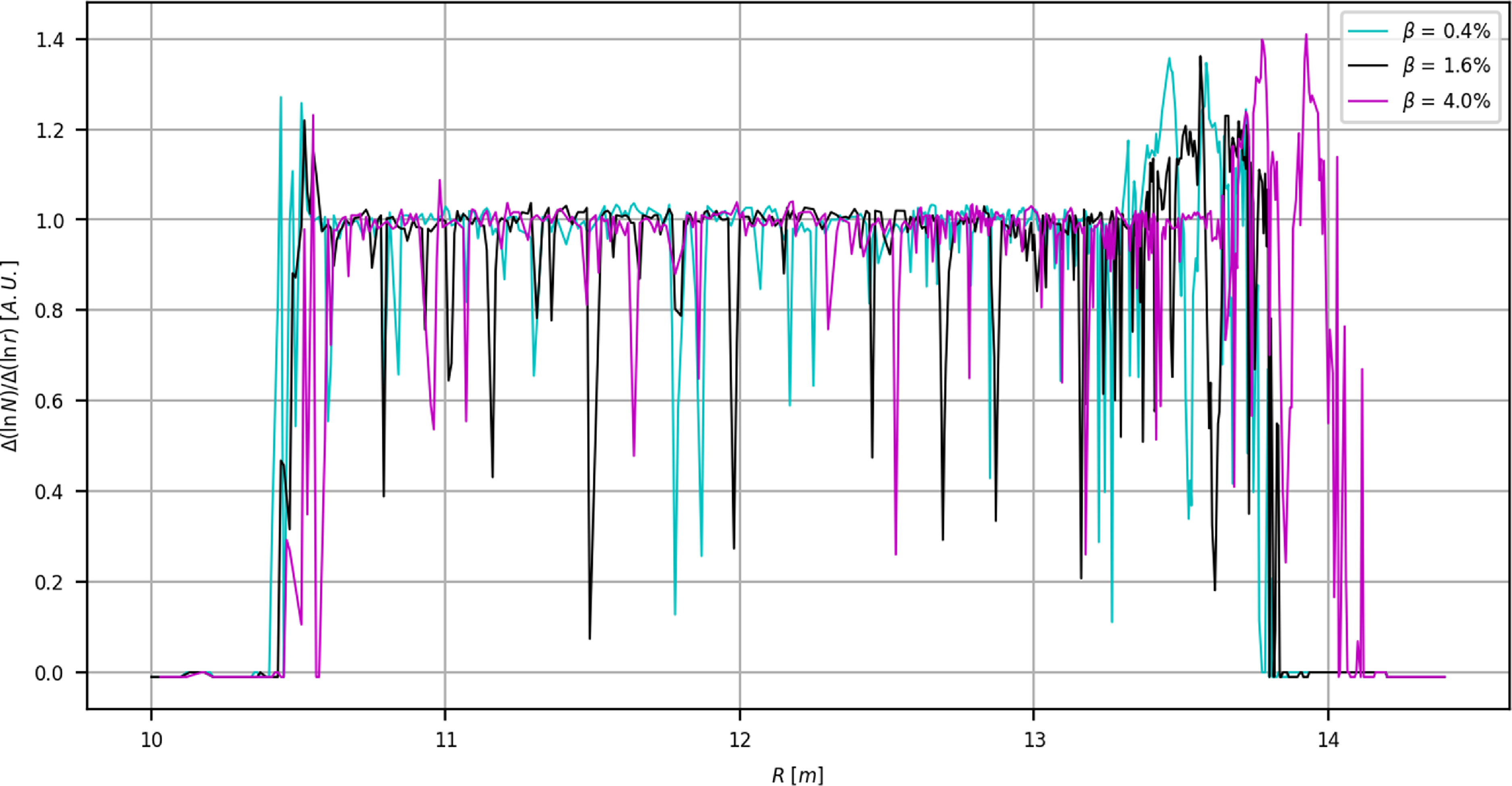
Figure 21. Fractal dimension for three values of $\beta$
based on HINT simulations with parabolic pressure profiles.
$\beta$
based on HINT simulations with parabolic pressure profiles.
Appendix D. SFINCS
The SFINCS code (Landreman et al. Reference Landreman, Smith, Mollén and Helander2014), which is used in this work, directly solves the drift-kinetic equation in general toroidal configurations. Furthermore, it includes the effects of the radial electric field which is important in the search for the ambipolar electron- and ion-root solutions consistent with thermodynamic considerations (Shaing Reference Shaing1984; Turkin et al. Reference Turkin, Beidler, Maaßberg, Murakami, Tribaldos and Wakasa2011). A single evaluation of SFINCS requires a definition of the plasma species profiles (temperatures and densities for each), the geometry of the configuration of interest, and details about the specific radial location and radial electric field value to use for the evaluation. The output of a single evaluation includes the radial fluxes of particles and heat, and the parallel flows. Here, several evaluations of SFINCS are performed at each radial location with a range of values of $E_r$
to bracket the ambipolar solution, where the radial current density,
$E_r$
to bracket the ambipolar solution, where the radial current density, $\langle \vec {J}\cdot \nabla \rho \rangle$
, equivalent to the charge-weighted sum of the radial particle fluxes
$\langle \vec {J}\cdot \nabla \rho \rangle$
, equivalent to the charge-weighted sum of the radial particle fluxes $\boldsymbol{\varGamma}$
over each plasma species
$\boldsymbol{\varGamma}$
over each plasma species $x$
, is 0:
$x$
, is 0:
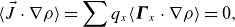 \begin{equation} \langle \vec {J}\cdot \nabla \rho \rangle =\sum q_x \langle \boldsymbol{\varGamma }_x\cdot \nabla \rho \rangle = 0, \end{equation}
where $q_x$
is the charge of species
$q_x$
is the charge of species $x$
and
$x$
and $\rho =\sqrt {s}$
, the square-root of the normalised toroidal flux. The bootstrap current is the charge-weighted sum of the parallel flows at the ambipolar field solution. It is possible for multiple stable ambipolar solutions to exist. Often referred to as ion-root (
$\rho =\sqrt {s}$
, the square-root of the normalised toroidal flux. The bootstrap current is the charge-weighted sum of the parallel flows at the ambipolar field solution. It is possible for multiple stable ambipolar solutions to exist. Often referred to as ion-root ( $E_r^{\rm i}$
) or electron-root (
$E_r^{\rm i}$
) or electron-root ( $E_r^{\rm e}$
), the parallel flows can be strongly modified or reduced in one regime or the other (and the influence on radial impurity transport is an important consideration). The root selected in the device is predicted by considering the minimisation of the generalised heat production (Shaing Reference Shaing1984; Turkin et al. Reference Turkin, Beidler, Maaßberg, Murakami, Tribaldos and Wakasa2011). At each radial location exhibiting multiple stable roots, the following integral is evaluated:
$E_r^{\rm e}$
), the parallel flows can be strongly modified or reduced in one regime or the other (and the influence on radial impurity transport is an important consideration). The root selected in the device is predicted by considering the minimisation of the generalised heat production (Shaing Reference Shaing1984; Turkin et al. Reference Turkin, Beidler, Maaßberg, Murakami, Tribaldos and Wakasa2011). At each radial location exhibiting multiple stable roots, the following integral is evaluated:
 \begin{equation} \int _{E_r^{\rm i}}^{E_r^{\rm e}}{\textrm{d} E_r \left ( Z_i \varGamma _i - \varGamma _e \right )}, \end{equation}
where $Z_i$
is the ion charge relative to the proton charge. The balance between the sum of the radial ion (i) and electron (e) currents determines which root is predicted. If the integral is positive, the ion-root is selected. The electron-root is preferred if the integral is negative.
$Z_i$
is the ion charge relative to the proton charge. The balance between the sum of the radial ion (i) and electron (e) currents determines which root is predicted. If the integral is positive, the ion-root is selected. The electron-root is preferred if the integral is negative.
A bootstrap current profile that is self-consistent with the plasma profiles can be established by a two-step process. In the first step, the VMEC input pressure profile is set to be consistent with the desired plasma temperature and density profiles, $p(s) = q\sum N(s)\cdot T(s)$
. The initial toroidal current profile is set to 0 or provided with some initial guess. VMEC is then allowed to converge. In the second step, SFINCS evaluations provide a new estimate of bootstrap current profile using the specified plasma density and temperature profiles along with the magnetic field and geometry information of the VMEC MHD solution. The toroidal current profile parameters in VMEC are then updated with this new estimate from SFINCS. By repeating the VMEC solution with improved estimates of the toroidal current profile provided by the SFINCS evaluations, a self-consistent estimate can be found after a few iterations. Specifically, the MHD solution and bootstrap current estimates are iterated (Watanabe et al. Reference Watanabe, Nakajima, Okamoto, Nakamura and Wakatani1992) until the toroidal current density,
$p(s) = q\sum N(s)\cdot T(s)$
. The initial toroidal current profile is set to 0 or provided with some initial guess. VMEC is then allowed to converge. In the second step, SFINCS evaluations provide a new estimate of bootstrap current profile using the specified plasma density and temperature profiles along with the magnetic field and geometry information of the VMEC MHD solution. The toroidal current profile parameters in VMEC are then updated with this new estimate from SFINCS. By repeating the VMEC solution with improved estimates of the toroidal current profile provided by the SFINCS evaluations, a self-consistent estimate can be found after a few iterations. Specifically, the MHD solution and bootstrap current estimates are iterated (Watanabe et al. Reference Watanabe, Nakajima, Okamoto, Nakamura and Wakatani1992) until the toroidal current density, $J_t(s)$
, is self-consistent, which is defined as the condition that the toroidal current enclosed within a flux surface,
$J_t(s)$
, is self-consistent, which is defined as the condition that the toroidal current enclosed within a flux surface, $I(s)=\int _0^s{\textrm{d}s J_t(s)}$
, in VMEC is consistent with the average parallel current
$I(s)=\int _0^s{\textrm{d}s J_t(s)}$
, in VMEC is consistent with the average parallel current $\langle \vec {J} \cdot \vec {B}\rangle$
calculated with SFINCS. Here,
$\langle \vec {J} \cdot \vec {B}\rangle$
calculated with SFINCS. Here, $s$
is the normalised toroidal flux. In equilibrium, these quantities satisfy
$s$
is the normalised toroidal flux. In equilibrium, these quantities satisfy
 \begin{equation} \frac {\textrm{d}I\left (s\right )}{\textrm{d}s} + \frac {\mu _0I\left (s\right )}{\langle B^2 \rangle } \frac {\textrm{d}p\left (s\right )}{\textrm{d}s} = 2\pi \frac {\textrm{d}\psi }{\textrm{d}s}\frac {\langle \vec {J} \cdot \vec {B}\rangle }{\langle B^2\rangle } \end{equation}
(see Appendix C of Landreman & Catto (Reference Landreman and Catto2012)). When the $L_1$
-norm of the change to the toroidal current profile between iterations divided by the
$L_1$
-norm of the change to the toroidal current profile between iterations divided by the $L_1$
-norm of the toroidal current profile is less than some tolerance (of the order of
$L_1$
-norm of the toroidal current profile is less than some tolerance (of the order of ${\sim} 1\,\%$
in our work), or after some limit on the number of iterations is reached, the toroidal current profile is considered to be self-consistent. The number of iterations required by VMEC and SFINCS to attain a self-consistent estimate of the bootstrap current varies depending on the starting equilibrium and grid parameters of the five-dimensional (5-D) phase space of the drift-kinetic equation expansion. The workflow of this process is shown in figure 22.
${\sim} 1\,\%$
in our work), or after some limit on the number of iterations is reached, the toroidal current profile is considered to be self-consistent. The number of iterations required by VMEC and SFINCS to attain a self-consistent estimate of the bootstrap current varies depending on the starting equilibrium and grid parameters of the five-dimensional (5-D) phase space of the drift-kinetic equation expansion. The workflow of this process is shown in figure 22.
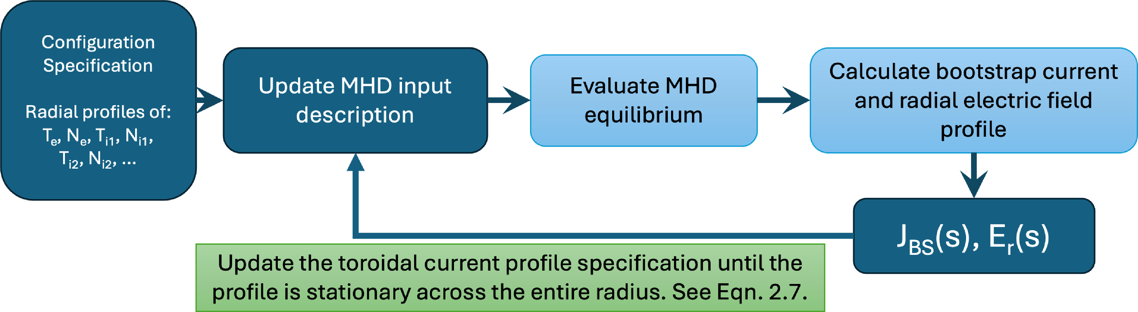
Figure 22. Workflow for calculating the self-consistent bootstrap current. Each iteration involves one MHD evaluation, and many evaluations of neoclassical fluxes and flows for the bootstrap current estimate. The loop continues until the toroidal current profile has converged to within some tolerance.
D.1 Parameter settings
The parameters listed in table 5 provide well-converged solutions for SFINCS evaluations for operating points listed in table 3. Convergence tests were performed for each of the parameters for low-, medium- and high-density cases.
Table 5. SFINCS numerical resolutions parameters.

Appendix E. COBRAVMEC
Ballooning modes are localised along a field line in regions of unfavourable curvature (Freidberg Reference Freidberg2014). The modes are destabilised when the pressure gradient, $p'=(\textrm{d}p)/(\textrm{d}s)$
, is above some threshold. Stabilisation occurs through magnetic field-line bending (Hegna & Nakajima Reference Hegna and Nakajima1998).
$p'=(\textrm{d}p)/(\textrm{d}s)$
, is above some threshold. Stabilisation occurs through magnetic field-line bending (Hegna & Nakajima Reference Hegna and Nakajima1998).
Ballooning stability is computed by solving the 1-D eigenvalue equation (Correa-Restrepo Reference Correa-Restrepo1978; Sanchez et al. Reference Sanchez2001)
 \begin{align} &\left [ \frac {d}{\textrm{d}\phi } \left [ P\left (\phi \right )\frac {d}{\textrm{d}\phi }\right ]+Q_1\left (\phi \right ) +\lambda R\left (\phi \right ) \right ] F\left (\phi \right ) = 0, \end{align}
where
 \begin{align} P &= B^\phi |\boldsymbol{k}_\perp |^2 / B^2, \end{align}
 \begin{align} R &=\frac {P}{\left ({B^\phi }\right )^2}, \end{align}
 \begin{align} Q_1 &= \frac {\epsilon ^2\beta _0 p' \kappa _s}{B^\phi } \\[10pt]\nonumber\end{align}
and the inverse aspect ratio is $\epsilon = a / R_0$
, where
$\epsilon = a / R_0$
, where $a$
and
$a$
and $R_0$
are the minor and major radii. Here,
$R_0$
are the minor and major radii. Here, $B^\phi$
is the toroidal contravariant component of
$B^\phi$
is the toroidal contravariant component of $\vec {B}$
,
$\vec {B}$
, $\boldsymbol{k}_\perp$
is the perpendicular wavevector and
$\boldsymbol{k}_\perp$
is the perpendicular wavevector and $\kappa _s$
is the normal curvature.
$\kappa _s$
is the normal curvature.
For the ballooning stability evaluations shown in figure 17, field lines on the flux surface where chosen to be centred on a 2-D mesh in the poloidal and toroidal directions. The field lines locations were separated by $18^\circ$
in the poloidal direction, starting at
$18^\circ$
in the poloidal direction, starting at $\theta =0$
. The lines were separated by
$\theta =0$
. The lines were separated by $6^\circ$
in the toroidal direction starting at the
$6^\circ$
in the toroidal direction starting at the $\varPhi =0$
location. Several radial surfaces were analysed, ranging from
$\varPhi =0$
location. Several radial surfaces were analysed, ranging from $s= 0.05$
to
$s= 0.05$
to $s=0.95$
in increments of
$s=0.95$
in increments of $0.05$
. The estimated number of helical wells included in the analysis permitted in the evaluation was selected from 1, 3 and 10, with 10 always providing the most restrictive limit of the stability.
$0.05$
. The estimated number of helical wells included in the analysis permitted in the evaluation was selected from 1, 3 and 10, with 10 always providing the most restrictive limit of the stability.
Appendix F. TERPSICHORE
The ideal MHD stability of magnetically confined plasmas is described by a variational formulation of the linearised equations of motion coupled with the continuity equation, an equation of state that governs the pressure evolution, Maxwell’s equations that includes Ampère’s law, and Ohm’s law. This was formulated by Bernstein et al. (Reference Bernstein, Frieman, Kruskal and Kulsrud1958) and serves as the basis for the development of computer codes to investigate tokamaks, reversed field pinches, stellarators and other confinement systems. For the stellarator configurations analysed here, we will assume an MHD equilibrium state with nested magnetic flux surfaces.
Here, the stability of a plasma is determined from the evaluation of the equation:
 \begin{align} \delta W_p + \delta W_v - \omega ^2 \delta W_k = 0 . \end{align}
The internal plasma potential energy is
 \begin{align} \delta W_p = \frac {1}{2}\int \int \int d^3x \big[Q_2^2 + \varGamma p(\nabla \cdot \vec {\xi })^2 + \vec {J}\times \vec {\xi }\cdot \vec {Q}_2+(\vec {\xi }\cdot \nabla p)(\nabla \cdot \vec {\xi })\big] , \end{align}
where $\vec {Q}_2=\nabla \times (\vec {\xi }\times \vec {B} )$
is the perturbed magnetic field and
$\vec {Q}_2=\nabla \times (\vec {\xi }\times \vec {B} )$
is the perturbed magnetic field and $\varGamma$
is the adiabatic index. The vacuum model presented in this paper is applicable to discretised vacuum domains, in particular, the mass-less, pressure-less and shear-less pseudo-plasma approach in TERPSICHORE. This pseudo-magnetic field and pseudo-displacement vector in the vacuum region are defined as
$\varGamma$
is the adiabatic index. The vacuum model presented in this paper is applicable to discretised vacuum domains, in particular, the mass-less, pressure-less and shear-less pseudo-plasma approach in TERPSICHORE. This pseudo-magnetic field and pseudo-displacement vector in the vacuum region are defined as $\vec {T}$
and
$\vec {T}$
and $\vec {\xi }_V$
, respectively, and the perturbed magnetic field vector potential in the vacuum region,
$\vec {\xi }_V$
, respectively, and the perturbed magnetic field vector potential in the vacuum region, $\vec {A}=\vec {\xi }_V\times \vec {T}$
, has no component parallel to
$\vec {A}=\vec {\xi }_V\times \vec {T}$
, has no component parallel to $\vec {T}$
(Schwenn et al. Reference Schwenn, Anderson, Cooper, Gruber and Merazzi1990). The magnetic energy in the vacuum region is
$\vec {T}$
(Schwenn et al. Reference Schwenn, Anderson, Cooper, Gruber and Merazzi1990). The magnetic energy in the vacuum region is
 \begin{align} \delta W_v = \frac {1}{2}\int \int \int {\textrm{d}^3 x [ \nabla \times (\vec {\xi _V}\times \vec {T})]^2} . \end{align}
A useful description of the kinetic energy is the expression
 \begin{align} \delta W_k = \frac {1}{2} \int \int \int { \textrm{d}^3 x \vec {\xi }\cdot \vec {\vec {\rho }}_M\cdot \vec {\xi }} , \end{align}
where $\vec {\vec {\rho }}_M$
is the dyadic tensor given by
$\vec {\vec {\rho }}_M$
is the dyadic tensor given by
 \begin{align} \vec {\vec {\rho }}_M = \nabla s \nabla s + \left (\psi _t'(s)\nabla \theta -\psi _p'(s)\nabla \phi \right )\left (\psi _t'(s)\nabla \theta -\psi _p'(s)\nabla \phi \right ). \end{align}
The eigenvalue of the system is $\omega ^2$
, with
$\omega ^2$
, with $\omega ^2 \lt 0$
indicating instability. The applications of the TERPSICHORE code rely on a model kinetic energy that annihilates the parallel component of the perturbed displacement vector. This allows the algebraic elimination of the plasma compression term in the energy principle. Consequently, the incompressibility constraint is automatically applied and implies that
$\omega ^2 \lt 0$
indicating instability. The applications of the TERPSICHORE code rely on a model kinetic energy that annihilates the parallel component of the perturbed displacement vector. This allows the algebraic elimination of the plasma compression term in the energy principle. Consequently, the incompressibility constraint is automatically applied and implies that $\nabla \cdot \vec {\xi }=0$
. The incompressibility constraint coupled with a model kinetic energy that annihilates the component of
$\nabla \cdot \vec {\xi }=0$
. The incompressibility constraint coupled with a model kinetic energy that annihilates the component of $\vec {\xi }$
parallel to
$\vec {\xi }$
parallel to $\vec {B}$
, through the choice of the dyadic
$\vec {B}$
, through the choice of the dyadic $\vec {\vec {\rho }}_M$
, reduces the linear ideal MHD stability problem to a partial differential equation with two unknowns, the component normal to the magnetic flux surfaces and a second bi-normal component. A Fourier decomposition of the perturbations in the Boozer magnetic coordinate system (Boozer Reference Boozer1981) and a radial discretisation with a hybrid finite element scheme further reduce the problem to a special block pentadiagonal matrix equation that is solved in the TERPSICHORE code with an inverse vector iteration method (Anderson et al. Reference Anderson, Cooper, Gruber, Merazzi and Schwenn1990). Vacuum pseudo-flux surfaces are constructed such that the geometry is continuously differentiable across the plasma vacuum interface into the vacuum domain. The structure of the matrix equation in the vacuum is identical to that in the plasma (Cooper Reference Cooper1992).
$\vec {\vec {\rho }}_M$
, reduces the linear ideal MHD stability problem to a partial differential equation with two unknowns, the component normal to the magnetic flux surfaces and a second bi-normal component. A Fourier decomposition of the perturbations in the Boozer magnetic coordinate system (Boozer Reference Boozer1981) and a radial discretisation with a hybrid finite element scheme further reduce the problem to a special block pentadiagonal matrix equation that is solved in the TERPSICHORE code with an inverse vector iteration method (Anderson et al. Reference Anderson, Cooper, Gruber, Merazzi and Schwenn1990). Vacuum pseudo-flux surfaces are constructed such that the geometry is continuously differentiable across the plasma vacuum interface into the vacuum domain. The structure of the matrix equation in the vacuum is identical to that in the plasma (Cooper Reference Cooper1992).
In a magnetically confined plasma, any perturbation must vanish at infinity. To approximate this condition, an axisymmetric conducting wall that hugs the major axis, yet is sufficiently far from the plasma vacuum interface, is prescribed on which the radial component of the displacement vector $\vec {\xi }_V\cdot \nabla s\equiv 0$
.
$\vec {\xi }_V\cdot \nabla s\equiv 0$
.
TERPSICHORE has been applied for approximately 35 years for Stellarator and some Tokamak applications. It has been benchmarked with the CAS3D code (Nührenberg et al. Reference Nührenberg, Boozer and Hudson2009) and with 3-D finite-n ballooning corrections (Cooper, Singleton & Dewar Reference Cooper, Singleton and Dewar1996).
F.1 Resolution and mode families
For the TERPSICHORE analysis performed in this work, the radial resolution covered 123 radial intervals in the plasma and 36 in the vacuum domain. In the course of the work, the radial resolution of some MHD solutions was increased up to 165 (164 radial intervals) to investigate the radial convergence of localised perturbations. The n= 0, n= 1 and n= 2 mode families were each explored. For a full description of the mode coupling that is implied by these families, please see Section 3 of Ardelea & Cooper (Reference Ardelea and Cooper1997). The Fourier mode window was adjusted to encompass a spectrum of nearly 19 poloidal modes and between 10 and 17 toroidal modes (depending on whether the toroidal mode number is even or odd) about the dominant Fourier mode. This is adequate to couple the instability structure with the spectrum that describes the equilibrium state. This resolution was acceptable for low and intermediate m,n mode number structures because the configuration studied has low magnetic shear. In devices with higher shear, a finer radial grid would be required.


 Open access